No category

Download User`s Manual

Transcript

Java Software for Bayesian ANOVA of
Microarray Data
BAMarray 3.0 User’s Manual
TM
November 6, 2008
Hemant Ishwaran
J. Sunil Rao
Udaya B. Kogalur
www.bamarray.com
2
CONTENTS
Contents
1
Overview
1.1 Background . . . . . . . . . . . . . . . . . . . . . . . . . . . . . . . . . . . .
1.2 Bayesian ANOVA for Microarrays (BAM) . . . . . . . . . . . . . . . . . . . .
4
4
5
2
Illustrative Examples
2.1 Stagewise Development of Liver Metastatic Colon Cancer: Multigroup Analysis
2.2 Human Gene Atlas: No Baseline Group . . . . . . . . . . . . . . . . . . . . .
2.3 Invariant Set Normalization: Batch Mode Scripting . . . . . . . . . . . . . . .
2.4 Outlier Detection: Spike-In Controls . . . . . . . . . . . . . . . . . . . . . . .
2.5 Time Course Analysis: Profile Identification . . . . . . . . . . . . . . . . . . .
2.6 Survival Analysis: Finding Genes Related to Short or Long-term Survival . . .
6
6
8
10
12
15
18
3
Software Details
3.1 Software Architecture . . . . . . . . . .
3.2 Installing and Uninstalling BAMarrayTM
3.3 What’s New in 3.0: Software Features .
3.4 System Requirements . . . . . . . . . .
3.5 Windows XP . . . . . . . . . . . . . .
3.6 Mac OS X . . . . . . . . . . . . . . . .
.
.
.
.
.
.
20
20
20
22
23
23
23
4
Data Formats and Importing Data Files
4.1 Supported Data files and Formatting Issues . . . . . . . . . . . . . . . . . . .
4.2 Illustrative Example (Bundled Data) . . . . . . . . . . . . . . . . . . . . . . .
4.3 Importing Data . . . . . . . . . . . . . . . . . . . . . . . . . . . . . . . . . .
24
24
24
24
5
BAMarrayTM Run Settings
26
6
Save and Restore Run Feature
29
7
The BAMarrayTM Graphical Suite
7.1 Data Plots for Assessing Model Assumptions . . . . . . . . .
7.2 More On Assuming Equal Variances Across Groups . . . . . .
7.3 Inferential Plots for Detecting Differentially Expressing Genes
7.4 Adding Gene Labels to Plots and Saving Gene Lists . . . . . .
7.5 Plotting Options and Using the Gene Tracking Facility . . . .
7.6 Rank Ordering Gene Effects . . . . . . . . . . . . . . . . . .
30
31
34
34
39
39
43
.
.
.
.
.
.
.
.
.
.
.
.
.
.
.
.
.
.
.
.
.
.
.
.
.
.
.
.
.
.
.
.
.
.
.
.
.
.
.
.
.
.
.
.
.
.
.
.
.
.
.
.
.
.
.
.
.
.
.
.
.
.
.
.
.
.
.
.
.
.
.
.
.
.
.
.
.
.
.
.
.
.
.
.
.
.
.
.
.
.
.
.
.
.
.
.
.
.
.
.
.
.
.
.
.
.
.
.
.
.
.
.
.
.
.
.
.
.
.
.
.
.
.
.
.
.
.
.
.
.
.
.
.
.
.
.
.
.
.
.
.
.
.
.
.
.
.
.
.
.
.
.
.
.
.
.
.
.
.
.
.
.
.
.
.
.
.
.
.
.
.
.
.
.
8
Some Useful Suggestions for Post-Processing Output
43
9
Appendix: Batch Mode Processing
45
10 Appendix: 64-bit Computing
48
CONTENTS
11 Appendix: Technical Details
11.1 The Multigroup ANOVA Model . . . .
11.2 CART Variance Stabilization of the Data
11.3 Rescaled Spike and Slab Models . . . .
11.4 Continuous Bimodal Priors . . . . . . .
11.5 Regularization: Zcut Values . . . . . .
11.6 The Zcut Multigroup Rule . . . . . . .
12 Acknowledgements
3
.
.
.
.
.
.
.
.
.
.
.
.
.
.
.
.
.
.
.
.
.
.
.
.
.
.
.
.
.
.
.
.
.
.
.
.
.
.
.
.
.
.
.
.
.
.
.
.
.
.
.
.
.
.
.
.
.
.
.
.
.
.
.
.
.
.
.
.
.
.
.
.
.
.
.
.
.
.
.
.
.
.
.
.
.
.
.
.
.
.
.
.
.
.
.
.
.
.
.
.
.
.
.
.
.
.
.
.
.
.
.
.
.
.
.
.
.
.
.
.
.
.
.
.
.
.
48
49
49
52
53
54
55
55
4
1
1
OVERVIEW
Overview
BAMarrayTM 3.0 (henceforth simply called BAMarrayTM ) is a graphically oriented, user friendly,
Java software package for the analysis of microarray data. The software is platform independent
with current solutions existing for Windows XP and Mac OS X operating systems. In addition
to its Java interface, the software can be run in an unattended Batch Mode using an XML script
file. BAMarrayTM implements the Bayesian ANOVA for microarray (BAM) methodology for
detecting differentially expressing genes in multigroup microarray experiments (see [1, 2, 3,
4]). As will be shown, the general methodology allows for many types of different modeling
strategies beyond classic multigroup designs, including: time course profiling, survival analysis,
invariant set normalization and certain styles of clustering.
1.1
Background
DNA microarray technology allows researchers to estimate the relative expression levels of
thousands of genes simultaneously over different time points, different experimental conditions,
or different tissue samples. It is the relevant abundance of the mRNA genetic product that provides surrogate information about the relative abundance of the cell’s proteins. The differences
in protein abundance are what characterize phenotypic differences between cells. Identifying
such differences (even at the mRNA level) can lead to insight about biological processes and
pathways that might be involved in a disease process as well as highlight new potential targets
for diagnostic and therapeutic development. See [5, 6, 7, 8] for more background on microarrays.
While potentially rich in information, microarray data pose a serious statistical challenge
due to the sheer volume of information being processed. It is typical to see data collected
on tens of thousands of mRNA transcripts from only a handful of samples. Moreover, the
amount of genomic information captured on arrays continues to scale up at tremendous rates.
For example, the new GeneChipR Exon ST array developed by Affymetrix contains over 1.4
million probe sets and over 5 million probes [9]. Contrasted with Affymetrix’s popular high
throughput array, the GeneChipR Human Genome U133 Plus 2.0 array, with roughly 54,000
probe sets, the new exon chip represents a 26-fold increase in data.
Scalability is not the only thorny issue in analyzing array data. Data analysis is further
complicated because of heterogeneity of gene-specific variances and correlation of expression
values due to biological effect or technological artifact. In fact, technical correlation is tightly
interrelated to scalability. As the amount of genomic information increases, so does technical
correlation. This is because of the high overlap existing in probe sets as chips become more
dense. For example, Affymetrix’s new Exon chip contains over 300,000 transcript clusters, of
which over 90,000 contain more than one probe set. As a transcript cluster measures information for a gene, there is significant overlap in data at the gene level.
Although many inferential questions are of interest, a key concern in analyzing microarray
data is the detection of differentially expressing genes between experimental groups. Traditional settings for this problem might include comparing gene expressions between control
1.2
Bayesian ANOVA for Microarrays (BAM)
5
samples and treatment samples, or between normal tissue samples and diseased tissue samples. However, many other interesting scientific questions can be recast under this framework.
Our sequence of examples, to be given shortly, will illustrate just how diverse a collection of
problems fall under this umbrella.
1.2
Bayesian ANOVA for Microarrays (BAM)
Recently, Ishwaran and Rao [2], building upon work in [1], introduced a method for detecting
differentially expressing genes between multiple groups termed Bayesian ANOVA for microarrays (BAM). This method recasts the statistical problem as a high dimensional model selection
problem, and uses a Bayesian hierarchical model designed for adaptive shrinkage. By using
model averaging, a way of accounting for model uncertainty, BAM provides gene effect estimates that are shrunken relative to maximum likelihood estimates in which primarily only the
non-differentially expressing gene effects are shrunken. This is a general phenomenon called selective shrinkage that enables BAM to optimally balance total false detections (the total number
of genes falsely identified as being differentially expressed) against total false non-detections
(the total number of genes falsely identified as being non-differentially expressed). Selective
shrinkage ultimately translates into more reproducible differential calls.
BAM’s ability to selectively shrink gene effects is an important form of regularization (sharing of information across genes) and is due to the use of what is called a rescaled spike and slab
model (see [3] for details). This model, in combination with a carefully selected continuous
bimodal prior (again, see [3]), enables BAM to use data across all genes and all experimental
groups to accurately estimate different levels of sparsity (the percentage of genes differentially
expressing over a specific experimental group) and then to selectively shrink gene effects based
on the estimated complexities. Equivalently, this procedure can be viewed as a penalization
method in which each gene effect has a unique penalty term that is adaptively estimated from
the data [2]. The idea of using model selection subject to regularization and penalization is in
contrast to methods based on protecting only false detection rates (most typically used for the
two group problem). While being able to pull out more obvious signal (low-lying fruit), these
approaches tend to be based on fairly elementary test statistics and often miss subtle changes in
order to guarantee false discovery protection.
The BAM estimation procedure is fully automatic and is based on a Gibbs sampling algorithm. Not only are regularized differential gene effects estimated, but so is an automatic
data adaptive cutoff value for determining which genes are differentially expressing. This cutoff value, for large enough sample sizes, has the theoretical property of delineating genes with
true differential expression from those genes with no differential activity [2]. This is crucial,
since determining an appropriate cutoff value is a critical aspect in searching for differential
expression (whatever the method being used).
Another important feature in analyzing microarray data is the ability to systematically deal
with heterogeneity of variances across genes and groups. Variance stabilization can lead to
tremendous gains in power and is another important aspect of regularization. This issue was
discussed in depth in [1, 2, 10]. BAMarrayTM incorporates a nonparametric Classification and
6
2
ILLUSTRATIVE EXAMPLES
Regression Tree (CART) clustering algorithm described in [10] to effectively deal with unequal
variances. Of note is that the procedure does not artificially dampen or amplify group differences across genes for the sake of attaining variance stabilization.
BAM’s success was first shown in [1] for the two group problem, but new work shows performance is amplified in multigroup problems [2]. Multigroup data refers to microarray data
collected over different experimental conditions or groups, such as data collected from distinct
stages of a disease process, or data collected from different tissues within an organism. In such
settings, it becomes more difficult to identify real patterns of gene expression changes across
groups from ones that are spurious noise using standard methods [2]. However, BAM’s regularization allows it to accurately extract signal from noise. This makes it possible to accurately
identify patterns of interest like disease progression genes which demonstrate marked expression changes over experimental stages. A good example (which we say more about shortly) are
hit-and-run genes which affect a biologic system for a certain amount of time and then whose
affect vanishes.
Importantly, the underlying theory for BAM has been extensively studied in [1, 2, 3]. This
provides a deep understanding of exactly why, and under what conditions, the BAM approach is
expected to be successful. A by-product of this is that tuning parameters, such as cutoff values
for identifying differentially expressing genes, are automatically set at optimal values suggested
by the theory. Automated tuning parameters are the default in BAMarrayTM , although override
customization is possible. See Section 5 for detailed discussion on Run Settings. The Appendix
contains a brief overview of some of the technical details and underlying theory of BAM.
2
2.1
Illustrative Examples
Stagewise Development of Liver Metastatic Colon Cancer: Multigroup Analysis
As our first illustration, we look at data from a large microarray repository of colon cancer
samples of various stages of tumor progression (data obtained from Dr. Sanford Markowitz of
the Ireland Cancer Center of Case Western Reserve University). All gene expression data were
compiled using high density 59K-on-one gene chips developed by EOS Biotechnology. These
are Affymetrix-derived chips with proprietary probe sets. The high density of probe sets reflects
known genes and ESTs (expressed sequence tags) as well as predicted exons.
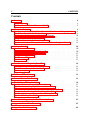
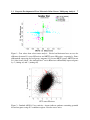
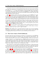
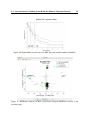
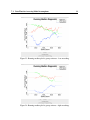
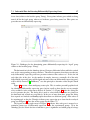
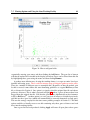
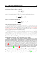
Figure 1 shows a BAM analysis of this database using four distinct tissue samples: Duke’s
B, C, D and liver METS. The Duke B samples represent Duke BSurvivors comprising patients
still alive from the time of initial diagnosis. These represent an intermediate stage of cancer and
represent our control (baseline) group for the analysis. Duke C samples represent a progressive
worsening of the disease as the cancer begins to invade deeper into the colon wall and spread to
nearby lymph nodes. The liver METS (METS) represent metastatic disease to the liver from the
original primary tumor. The Duke D samples represent the deposit left over in the colon after
liver metastasis. Plotted in the figure are BAM estimated gene differential effects called Zcut
2.1
Stagewise Development of Liver Metastatic Colon Cancer: Multigroup Analysis
7
Figure 1: Zcut values from colon cancer analysis. Vertical and horizontal axes are tests for
difference between D’s versus BSurvivors and METS versus BSurvivors, respectively. Genes
differentially expressing for both groups (magenta); D’s but not METS (green); METS but not
D’s (blue); none (black). Also indicated are C versus BSurvivors differentially expressed genes
by 4 (turning on) and O (turning off).
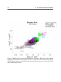
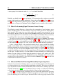
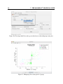
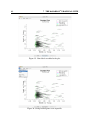
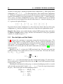
Figure 2: Standard ANOVA Z-test statistics. Arrows indicate quadrants containing potential
hit-and-run genes using 95% confidence regions. Note the excess noise.
8
2
ILLUSTRATIVE EXAMPLES
values for comparing the METS and D’s to the BSurvivors (x and y axes respectively). Also
overlayed on the plot are triangles oriented either up or down for identifying genes turning on or
off for stage C relative to the BSurvivors. In the figure we have used color to highlight stagewise
gene effects of biologic interest. Points colored in magenta are genes with significant differential
expression across the D’s and METS — either being turned on or turned off relative to the
BSurvivors. For example the small cluster of magenta triangles in the bottom-left quadrant
indicate genes that turn off throughout the C, D and METS samples. Data points colored in
green and blue indicate genes that are significant (in either direction) for only the stage D’s but
not the METS or only for the METS and not the stage D’s, respectively. In particular, green
points that hug the y-axis are those showing significant changes from BSurvivors to D’s but
whose METS expression resemble the BSurvivors. These are hit-and-run genes of particular
importance since they have a very specific early effect only.
Of particular note is the fact that statistical cutoffs and classification of genes are automatically determined from Zcut values using an automatic data adaptive Zcut rule (see the Appendix
for details). This frees the user from making difficult and arbitrary decisions regarding significance. Plots like Figure 1, which we refer to as multigroup Zcut scatter plots, are part of the
graphical suite available in BAMarrayTM . We will say more about graphics later in Section 7.
Standard maximum likelihood estimates (Z-tests) from a traditional ANOVA models provide a strikingly different plot (Figure 2). Especially apparent is the ellipsoid nature of the
figure. As was shown in [2], this is due to a regression to the mean effect caused by the correlation between the Z-statistics – in this case, for the METS versus BSurvivors and D versus
BSurvivors genewise effect estimates. Regression to the mean inflates false detections and
makes it more difficult to delineate signal from noise. Notice how difficult it is to identify any
hit-and-run candidates. Early hit-and-run genes might be the ones in the quadrants indicated
by the two arrows, but it is not so clear. This type of effect is clearly absent in Figure 1 and
demonstrates the benefits of shrinkage.
2.2
Human Gene Atlas: No Baseline Group
In the colon cancer example, we set things up to compare the various stages of colon cancer
(our group label) against the early onset stage BSurvivors group (our baseline group) – in a
sense, asking the question “what makes a good tumor go bad?”. In this case, differential expression refers to differences in gene expression values relative to the BSurvivors, our baseline
measurement. However, there are many interesting examples where there is no baseline group.
In such settings, a slightly different approach is needed, as differential expression now refers to
large absolute expression values. In other words, is the observed expression value significantly
different than zero? We refer to such examples as no baseline multigroup designs. It turns out
that there are a surprsing number of examples that can me made to fit under this framework.
BAMarrayTM includes a special option called no baseline specifically to handle such situations.
The following is an example illustrating a no baseline analysis (see Section 5 for how to
set this option within the software). For our example we consider the human gene atlas data
from [11]. We use the Human U133A–GNF1H, MAS 5.0 processed data; one of several variants
2.2
Human Gene Atlas: No Baseline Group
9
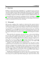
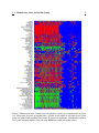
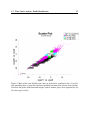
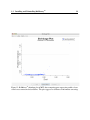
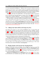
Figure 3: Human gene atlas. Vertical axis corresponds to tissue type, horizontal axis are probe
sets. Red points are genes up-regulated for a specific tissue relative to all other tissues; green
points are genes down-regulated; blue points are genes not significant. Classification based on
Zcut values and data adaptive Zcut rule using BAMarrayTM with no baseline option.
10
2
ILLUSTRATIVE EXAMPLES
of the database found at http://symatlas.gnf.org. In total there are 33,689 probe sets for each
of 158 chips in this dataset. The 33,689 probe sets represent a custom designed compilation of
Affymetrix Human U133A probe sets (22,283) as well as special GNF1H probe sets (22,645).
The 158 chips represent 82 groups of various human tissue type obtained from a diverse panel
of 79 individuals. No one group (tissue type) had more than two chips within it. See [11] for
details.
It is interesting to look for differences as well as similarities in gene expression values across
tissue types. For this purpose, we created what can be thought of as a “no baseline dataset”,
defined as follows. For each group, we computed the median expression value for a gene. For
tissues queried by only 1 chip, this amounts to simply using the expression value for a gene.
We then took this baseline median value and subtracted it from the expression value for the
gene from each of the remaining chips not in this tissue group. This was then repeated for all
genes for each of the 82 groups. The no baseline dataset contains the same number of groups
as the original data, namely 82, but the number of “new chips” within a group is considerable
expanded. In fact, each group in this new dataset contains either 157 new chips (a group with
only 1 chip originally) or 156 new chips (a group with 2 chips originally). In total there were
12,797 new chips and 33,689 probe sets for each chip in the new data.
Figure 3 records the results from a BAMarrayTM analysis invoking a no baseline option. Note
that once again genes are classified as being up-regulated or down-regulated by our automatic
data adaptive Zcut rule. The analysis is based on the top 10% of significant genes. For more
details, consult [12].
2.3
Invariant Set Normalization: Batch Mode Scripting
One of the important new features of BAMarrayTM is that it can be run in Batch Mode. This
makes it possible to configure and run BAMarrayTM using an XML batch file. Furthermore, one
can wrap the Batch Mode call to BAMarray in a custom R script, that allows the user to interface
BAMarrayTM with different types of software. We illustrate this by an example which shows how
to interface BAMarrayTM with Bioconductor to create a customized invariant set normalization
procedure.
The implementation for our example consists of several components. There is an R script,
a command shell script invoking BAMarrayTM in Batch Mode, and finally the Batch Mode
BAMarrayTM XML file containing data. (The various options and arguments available in Batch
Mode will be discussed later in the Appendix.)
Because implementation is rather involved, we will just summarize the main steps. The
main steps initiated by the script are as follows:
1. The user is prompted at the terminal level for information about the data and the type of
normalization desired.
2. An R file is then automatically run in batch mode. This code calls Biconductor and
normalizes the data. The normalized data is written to a text file.
Invariant Set Normalization: Batch Mode Scripting
11
10
5
eye7
eye7
eye7
eye45
eye45
eye45
eye28
eye28
eye28
eye21
eye21
eye21
eye14
eye14
eye14
eye0
eye0
eye0
0
Normalized Quantiles
15
2.3
Chips
8
6
4
2
eye7
eye7
eye7
eye45
eye45
eye45
eye28
eye28
eye28
eye21
eye21
eye21
eye14
eye14
eye14
eye0
eye0
eye0
0
Normalized Quantiles
10
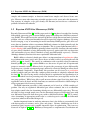
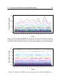
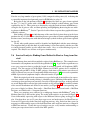
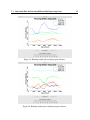
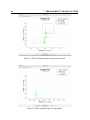
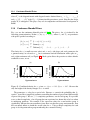
Figure 4: MAS 5.0 normalized EOM data. Vertical axis are the percentile values for the normalized data (percentiles range from 2 to 98). Each line corresponds to a specific percentile for
each of the 18 chips. Notice how the lines are fairly bumpy, indicating a sub-par normalization.
Chips
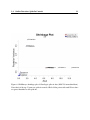
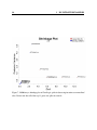
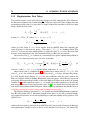
Figure 5: Normalization of EOM data using invariant probesets identified by BAMarrayTM .
12
2
ILLUSTRATIVE EXAMPLES
3. BAMarrayTM is called in batch mode. An XML batch file (created in the previous step)
is read and the normalized data is analyzed. Significant genes found by BAMarrayTM are
automatically written to a text file.
4. The output file containing the significant genes is parsed in R and a list of non-significant
genes is obtained. An invariant set normalization procedure is then applied (in R) to the
set of non-significant genes. The invariant set normalized data is written to a text file.
We illustrate this method using time course data. The data consists of limb and extraocular
(EOM) muscles pooled from multiple rats at 6 distinct time points (day 0, day 7, day 14, day 21,
day 28 and day 45). The data was collected in such a way to obtain three independent replicates
of age and muscle groups. This gave a total sample size of 6 × 3 × 2 = 36. The tissue data
was queried using the Affymetrix GeneChipR Rat Genome U34 Array Set (RG-U34A). The set
includes 8,799 probe sets reflecting known genes and EST clusters. The CEL files for the data
are available at the National Center for Biotechnology Information (NCBI) Gene Expression
Omnibus (GEO) data repository under series record accession number GSE903.
For our example we focus on the subset of the data comprising the EOM tissues (18 chips
in total). We took the time point “day 0” to act as the baseline in our multigroup analysis.
Figure 4 shows the normalized data using the MAS 5.0 normalization procedure available within
Bioconductor (invoked using the “mas5()” function). The normalization of the data, as well as
the plot, was generated automatically in our Batch Mode procedure. The genes found nonsignificant from a BAMarrayTM multigroup analysis using the normalized data were then used to
implement an invariant set normalization procedure, defined as follows (again, all of these steps
were performed automatically in the Batch Mode procedure). First, MAS 5.0 gene expression
values were clustered into percentiles ranging from 1 through 100. Then, within a specific
percentile, the average value of the invariant genes within the percentile was computed for each
chip. This value was then used to rescale all genes within a given percentile for each chip.
Essentially one can think of this as a local rescaling transformation.
The results of the invariant set normalization are given in Figure 5. Clearly the method has
improved overall consistency between chips. We happily encourage the user to experiment with
their own invariant methods using our script file as a template (available on request).
2.4
Outlier Detection: Spike-In Controls
The following example illustrates how BAMarrayTM can be used for outlier detection. This is
another example of a no baseline analysis, but here, unlike in the human gene atlas example of
Section 2.2, there is only one group.
Our examples uses the well known GeneLogic spike-in data. Here each of 11 control
cRNA’s were spiked-into a hybridization mix containing background AML tumor cell lines.
Each hybridization mixture was hybridized to multiple Affymetrix U-95A GeneChipR arrays.
The concentrations used for spike-ins were 0.5, 1, 1.5, 2, 3, 5, 12.5, 25, 37.5, 50, 75, and 100
pM, arranged in a Latin square experiment. In total there were 32 arrays, with each array containing 12,626 probe sets. See [13] for details (the data we consider is described in Table 2 of
that manuscript).
2.4
Outlier Detection: Spike-In Controls
13
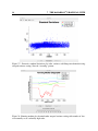
Figure 6: BAMarrayTM shrinkage plot of GeneLogic spike-in data (MAS 5.0 normalized data).
Note that 9 of the top 12 genes are spike-in controls. Blob of blue points with small Zcut values
are genes identified as non-spike-ins.
14
2
ILLUSTRATIVE EXAMPLES
Figure 7: BAMarrayTM shrinkage plot of GeneLogic spike-in data using invariant set normalized
data. Notice now that all of the top 11 genes are spike-in controls.
2.5
Time Course Analysis: Profile Identification
15
A no baseline dataset was created by taking each gene expression value on an array (obtained
using MAS 5.0 normalization) and subtracting the median expression value for the gene using
the remaining 32 − 1 = 31 arrays (for convenience we have posted the data on our website).
A one group analysis with no baseline was then fit using BAMarrayTM to identify differentially
expressing genes Note that because of the way we have defined our no baseline data, genes with
differential behavior indicate spike-ins.
Figure 6 is a shrinkage plot from the analysis. Such plots are part of the BAMarrayTM graphical suite (see Section 7) and are used for identifying differentially expressing genes. Notice,
in particular, the up-regulated genes highlighted with red points. Their labels identify them as
spike-in control genes (being able to label specific genes is a feature we will talk more about
later). In fact, 9 of the top 12 genes (going from right to left in terms of decreasing Zcut values)
are spike-ins. Also notice the blob of blue points with near zero Zcut values and small posterior
variances. These represent genes identified as non-spike-ins. The small Zcut values seen here,
and the correct identification of almost all of these genes, is a direct consequence of the selective
shrinkage property of BAM we discussed earlier.
Figure 7 is the same analysis, but now applied to data normalized using the invariant set
method discussed in Section 2.3. The normalization has helped to further improve accuracy.
Notice now that the top 11 genes are the 11 spike-in controls.
Remark 1. The shrinkage plot is a powerful automated tool that can be used for identifying
differentially expressing genes. It applies not only to the specific example considered here, but
to multigroup problems in general. We will say more about this plot later in Section 7.
2.5
Time Course Analysis: Profile Identification
We return to the time course data discussed in Section 2.3. We again focus on the EOM data
but now consider the problem of identifying genes with specific time profile behaviors. We
illustrate how this problem can be recast as a multigroup problem, similar to the colon cancer
example of Section 2.1, and demonstrate how a multigroup Zcut scatter plot can be used to
identify specific time course profiles. We emphasize that independence over time is a special
feature of this data that makes it amenable to such an analysis. That is, even though data was
collected over different time points, tissue samples were obtained by sacrificing the animal.
Thus the tissue samples, and array data, are independent over time.
For our analysis we use the invariant set normalized data of Section 2.3. The baseline group
for our analysis are tissues collected at day 0 of the study. In this case, differential expression
is measured with respect to time 0, and a gene found to be up or down regulated at a later time,
represents a gene whose expression value has increased or decreased over time.
Figures 8 and 9 are the multigroup Zcut plots obtained using BAMarrayTM . One interprets
the plots in a similar fashion as the colon cancer analysis (recall Figure 1). For example, the
green points in Figure 8 hugging the vertical axis represent genes whose expression values are
the same at day 7, but then become either up regulated, or down regulated, at day 14. The blue
points, on the other hand, are genes that are up or down regulated at day 7, but then turn off.
16
2
ILLUSTRATIVE EXAMPLES
Figure 8: Multigroup Zcut scatter plot for EOM time course data. Red points in left quadrant
highlighted by labels are down regulated for days 7, 14 and 21 relative to the baseline, day 0.
Note that points with up or downward triangle symbols indicate genes up or down regulated for
day 21 with respect to day 0.
2.5
Time Course Analysis: Profile Identification
17
Figure 9: Many of the same labeled points show up in the lower quadrant for days 21 and 28,
thus identifying these as genes that are down regulated for all time points relative to the baseline.
Note here that points with downward triangle symbols indicate genes down regulated for day
45 with respect to day 0.
18
2
ILLUSTRATIVE EXAMPLES
Note the very large number of green points (1,019) compared to blue points (69), indicating that
a potentially important developmental stage for EOM kicks in at day 14.
Red points in the left quadrant of Figure 8 highlighted by labels are genes down regulated
for days 7, 14 and 21 (points with a downward oriented triangle symbol indicate genes down
regulated for day 21). These points were obtained by using the zoom-in feature of BAMarrayTM ,
saving the list of genes to a file, and then uploading and highlighting them using the new tracking feature in BAMarrayTM . Section 7 provides details of how to operate these graphical features
within the software.
Now looking at Figure 9, we find that many of the same labeled points show up in the lower
quadrant for days 21 and 28, thus identifying them as genes that are down regulated throughout
the time course (note that points with downward triangle symbols indicate genes down regulated
for day 45).
Clearly, other profile patterns could be identified and highlighted with the same technique.
The important thing is that this kind of profile hunting is done interactively with the user able
to visually interpret profiles over the whole time course. Also, no ad hoc filtering of genes is
required. The analysis uses all data on all genes simultaneously.
2.6
Survival Analysis: Finding Genes Related to Short or Long-term Survival
We now illustrate how survival data might be explored using BAMarrayTM . The example comes
from mantle cell lymphoma survival data first published in [14]. A goal of the experiments was
to use gene expression data to predict the length of survival of mantle cell lymphoma (MCL)
patients. The data consists of 8810 cDNA elements for 92 MCL patients and is available at
http://llmpp.nih.gov/MCL. Of the 92 MCL patients, death times of 64 patients were observed,
while 28 patients were censored. Lymphochip cDNA microarrays ( [15]) were used to quantitate
mRNA expression in lymphoma samples extracted from the 92 patients.
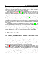
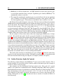
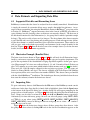
While the original goal of the experiment was to predict length of survival based on expression data, another avenue worth pursuing is identifying genes exhibiting differentially expression between short and long term survivors. In order to explore this question, we first generated
an overall Kaplan-Meier survival plot (with standard errors) in Figure 10. We took this estimate
of the survival distribution and divided it into tertiles (see Figure 10). The corresponding samples were re-labeled as follows: First tertile = ShortTerm Survivors; Second tertile = MidTerm
Survivors; and Third tertile = Longterm Survivors.
These new groupings were analyzed in a multigroup format with BAMarrayTM using the
Midterm Survivors as the baseline group. The results of the analysis are presented in Figure 11.
Genes differentially expressing with respect to the Midterm Survivor group are flagged in the
plot. Note how there are are 32 genes that seem to over and underexpress for ShortTerm survivors and 212 genes who do the same for LongTerm survivors. Also, notice how three genes (in
magenta) are differentially expressed for both ShortTerm and LongTerm survivors as compared
to MidTerm survivors. Clearly this type of analysis can give a very intuitive understanding as
to how gene expression relates to survival for MCL patients.
2.6
Survival Analysis: Finding Genes Related to Short or Long-term Survival
19
Mantle Cell Lymphoma Data
Survival Probability
Time (months)
Figure 10: Kaplan-Meier survival curve for MCL data with tertile boundaries identified.
Figure 11: BAMarrayTM analysis of MCL survival data using the MidTerm survivors as the
baseline group.
20
3
SOFTWARE DETAILS
BAMarrayTM can also be used to probe the potential validity of censoring assumptions. Typically in survival analysis settings, it is assumed the censoring mechanism is random and noninformative – that is, unrelated to the outcome of interest. However, it is not unusual for this
assumption to be suspect. For instance, informative censoring can occur if dropouts from a
study occur for reasons related to survival time (eg. illness). Alternatively, patients who experience adverse reaction to treatment may withdraw from a study which can introduce informative
censoring unless the adverse reaction is considered independent of the survival time of interest.
Typically it is nearly impossible to test for informative censoring since the necessary components of testing are not always available in clinical data. However, with gene expression data,
it is possible to informally probe whether censored observations tend to have a systematically
different set of gene expression profiles than uncensored observations. If so, then this might
lead one to conclude that since gene expressions are likely related to many unobserved competing risks, that informative censoring might be at play. To explore this possibility with the
MCL data, we simply recoded the data into two groups: Censored and Uncensored and then ran
a two-group BAMarrayTM analysis to compare gene expression profiles. As indicated by Figure 12, the BAMarrayTM inferential shrinkage plot (to be discussed in Section 7), finds no genes
with significantly different expression levels for the censored observations.
3
3.1
Software Details
Software Architecture
BAMarrayTM is a stand-alone platform-independent Java application. Solutions currently exist
for Windows XP, Mac OS X (ppc and i386). More will be added as demand necessitates. A
native code C library is at the core of the product. This library implements the BAM algorithm
and consists of several components executed in the following order:
Data pre-processing −→ Data variance stabilizing transformation −→ Gibbs sampler.
A graphical user interface surrounds the native code library and allows the user to interact with
the library and conduct customized data analysis.
3.2
Installing and Uninstalling BAMarrayTM
BAMarrayTM is available for download in the form of a compressed file installation package.
Detailed instructions for download and installation can be found at www.bamarray.com. The
installation package should be extracted into a directory of the users choice. The resulting
package will reside in USERHOME/BAMarray/
Uninstalling BAMarrayTM is as straightforward as the install process. The user simply deletes
the USERHOME/BAMarray directory in which the package was extracted.
3.2
Installing and Uninstalling BAMarrayTM
21
Figure 12: BAMarrayTM shrinkage plot of MCL data comparing gene expression profiles of censored versus uncensored observations. The plot suggests no evidence of informative censoring.
22
3
SOFTWARE DETAILS
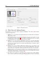
Figure 13: The main console.
3.3
What’s New in 3.0: Software Features
The following is a list of key features contained in BAMarrayTM 3.0. We use a ♠ to indicate
features new to this release.
1. BAMarrayTM is a user friendly Java application that runs on the Mac OS X, and Windows
XP operating systems.
2. Full multigroup analysis for an unlimited ♠ number of groups can be handled. Overlay
multigroup plots (similar to Figure 1) are available for visualizing how genes are mapped
to specific pattern types of differential expression across groups.
3♠. BAMarrayTM can be run unattended in Batch Mode initiated by a script file. Batch Mode
can process several data files sequentially and save the resulting analysis to disk. Writing
custom designed scripts allow users to interface with different types of software, such as
Bioconductor, and R.
4♠. BAMarrayTM has a Save and Restore Run feature allowing users to save results of a run
for retrieval at a later time. Saved runs can also be initiated in Batch Mode. This unique
feature allows users to batch files and then come back later and restore saved run states.
5. Graphical zoom-in and lassoing tools enable the user to interactively generate lists of
differentially expressing genes. Zoomed windows can be moved through either forwards
or backwards (similar to using a web browser) ♠.
6. Gene labels can be toggled on or off allowing genes of interest to be readily identified.
Genes of interest (such as those making up a biological pathway of interest) can be high-
3.4
System Requirements
23
lighted using a drop down list or populating a tracking list from gene labels found in an
existing file ♠.
7. Graphical plots for assessing the underlying assumptions of the model are included as part
of the graphics suite. This includes a new running median plot for rigorously assessing
the quality of the CART variance stabilizing procedure ♠.
8. A “no baseline” experimental design option is available for expanding the scope of multigroup models that can be fit.
9. Unequal variances across genes and experimental groups are systematically handled by
an automated pre-processing step that does not artificially dampen or amplify group differences across genes (as seen with other transformations, such as logarithms).
10. Figures can be saved as publication quality color graphics.
11. Gene lists of interest can be exported as text files for further exploration using other
software. This step can be fully automated using Batch Mode.
12♠ . Supports JRE 1.6x.
13♠ . Supports true 64-bit processing.
3.4
System Requirements
The minimum hardware requirements are primarily dependent on the size of the data sets that
the user plans to analyze. In general, we would recommend as a minumum:
• 512 MB RAM
• 100 MB free disk space on hard drive.
3.5
Windows XP
• Windows XP Service Pack 2.
• In some rare cases you might need to install the Java Platform, Standard Edition Runtime Environment Version 1.6x (also known as JRE 6). See http://java.sun.com for more
details. Note: to check if Java is already installed open a Command Prompt Window
(”Program Files -> Accessories -> Command Prompt”) and type ”java -version”. The
system should respond with ”1.6.x”.
3.6
Mac OS X
• 10.4 (Tiger) or 10.5 (Leopard).
• Note that the necessary Java Runtime Environment will already be installed on these
operating systems.
24
4
4
Data Formats and Importing Data Files
4.1
DATA FORMATS AND IMPORTING DATA FILES
Supported Data files and Formatting Issues
BAMarrayTM assumes that the data to be analyzed has been suitably normalized. Normalization
is simply the removal of systematic effects across samples that might bias inference. An example of how to normalize data using the Batch Mode feature in BAMarrayTM was given earlier
in Section 2.3. BAMarrayTM supports microarray data in the form of an EXCEL spreadsheet or
space-delimited text file (missing values are however not currently allowed). The first row of
the file should contain class label information (i.e., the group label to which a particular sample
belongs). This can be coded as letters and (or) integers. The first column of the dataset contains
a gene label ID and is used for plotting and reporting purposes. Each subsequent entry following the first column is a suitably normalized gene expression measurement. There must be one
row per gene, with each column representing a measurement for the sample identified in the
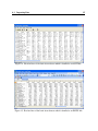
first row. Figures 14 and 15 show the first few rows of an example dataset (see below for more
details) in text and EXCEL formats respectively.
4.2
Illustrative Example (Bundled Data)
The brain tissue dataset shown in Figures 14 and 15 (this will used for all illustrations henceforth) is a microarray experiment studying hippocampal aging and cognitive impairment. The
goal of the experiment is the identification of aging-dependent cognitive decline gene expression. Hippocampal CA1 tissue was collected from 4, 14, and 24 month old male Fischer rats
after 7 days training on a water maze which included object memory task (see [16] for details).
There were 10, 9 and 10 samples collected for the respective age groups. The age groups are
labeled as Young, Middle, and Aged. The data are available at the Gene Expression Omnibus
data repository under series record accession number GSE854. This dataset comes pre-bundled
with the default BAMarrayTM installation. The default input directory (initialized when the user
first starts the software) contains the brain tissue dataset.
4.3
Importing Data
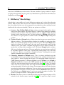
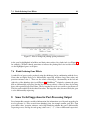
To open a microarray dataset, click New under the File menu of the BAMarrayTM main console
and browse for the data. Once the file is found, click to highlight it, then click the Open button
at the bottom of the Open File dialog box. Another dialog box will appear prompting for the
groups to be used in the analysis. (see Figure 16 which shows the dialog box for the brain tissue
data). Groups can be added or removed by using the Add and Remove buttons respectively.
Alternatively, for data with many groups, the user can select all groups (using SHIFT+END,
or CTRL-A), or any subset (using SHIFT PAGEUP, SHIFT PAGEDN, SHIFT ARROWUP,
SHIFT ARROWDN), instead of having to click on each group one at a time. All “standard”
navigation keys can be used.
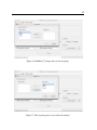
Figure 17 shows the brain tissue dataset where all three groups have been chosen. After
the groups have been selected, clicking OK reads in the data and a notification appears on the
4.3
Importing Data
Figure 14: First few lines of the brain tissue dataset which is bundled as an ASCII file.
Figure 15: First few lines of the brain tissue dataset which is bundled as an EXCEL file.
25
26
5
BAMARRAYTM RUN SETTINGS
status bar of the BAMarrayTM main console. File name, number of groups, number of samples
per group and total number of genes (probe sets) information are provided once the file has been
completely read (Figure 18).
5
BAMarray Run Settings
TM
After the data is successfully read, several different run options can be selected from the main
console. Many of these values are preset at well chosen default values and do not necessarily
have to be adjusted (in fact, users are recommended not to adjust these values until they become
familiar with the software and method). The key run options are as follows:
(a) Accuracy: Low, Medium, High and Super settings correspond to the number of iterations for the Gibbs sampler. The Gibbs sampler is a Monte Carlo method for estimating
parameter values of interest. The more iterations used (i.e., Super vs Low), the more
accurate, but the longer the run time. For data exploration, a Medium setting will suffice. However, it is good practice to confirm results at the High or Super setting when
possible.
(b) Variance: Equal and Unequal settings. Expression values for genes are expected to have
different variances. This option indicates whether the variability of expression values
differs over experimental groups and genes or only over genes. The default Equal option
implies the variance for a given gene is the same across experimental groups, but that
variances across genes differs. Graphical diagnostic plots (to be discussed shortly) are
provided for assessing if this assumption is met. The option Unequal implies variances
differ across both groups and genes. For many applications, an equal variance model will
be reasonably satisfied. Power gains, especially with smaller sample sizes, will result
in such cases. However, we provide an example in Section 7 showing when an equal
variance assumption across groups is unrealistic.
(c) Clustering: Automatic and Manual settings. This is a variance stabilization step that
systematically removes gene specific mean-variance trends, resulting in data with variances equal to 1 across all groups and all genes. The underlying method is based on a
CART clustering approach. A different algorithm is used if Variance is set at Equal or
Unequal. In both cases, however, the CART algorithm has the important property that
it does not alter the original signal to noise ratio of the data [10]. In fact, we strongly
advise users not to pre-process their data using transformations like logarithms because
such transformations do not have this feature. Our recommendation is to let the clustering
procedure deal with variance stabilization. Users are advised to not pre-process their data
using logarithms and always use this procedure with the Automatic default option on.
For advanced users a Manual option is used to pre-specify the number of clusters. We
provide an example in Section 7 showing how to use this feature.
(d) Baseline: This allows the user to define the baseline group for comparison purposes. The
rationale for the baseline group is provided in [1, 2]. It is typical to assign a control
27
Figure 16: BAMarrayTM prompts the user for the groups.
Figure 17: How to pick groups to be used for the analysis.
28
5
BAMARRAYTM RUN SETTINGS
Figure 18: File information is provided once the data is read.
Figure 19: “Young” group picked as the baseline.
29
group or perhaps a normal or preliminary disease state as the baseline group. Our colon
cancer example of Section 2.1 used BSurvivors for the baseline, whereas in the brain
tissue dataset the Young group serves as the baseline (see Figure 19). For time-course
data the zero time point might be the most sensible baseline choice (as in Section 2.5).
A No Baseline option, as used in the examples of Sections 2.2 and 2.4, is also available.
This option is accessible under the Tools menu on the main console under Baseline Option. Clicking on No Baseline Selection enables a no baseline analysis for the session
(in subsequent fresh sessions the No Baseline Selection is automatically reset to its default). As discused earlier, no baseline means that each gene effect is being tested against
a null value of zero (i.e. no detectable effect at all) rather than against a defined baseline
group. Note that when the No Baseline Selection is clicked, the select group menu under
Baseline on the main console is grayed out.
Clicking Run initiates the analysis. A progress bar at the bottom of the BAMarrayTM main
console indicate how long the Gibbs sampler will take and when the analysis has successfully
completed.
6
Save and Restore Run Feature
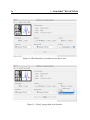
A new feature in BAMarrayTM 3.0 are the Save Run and Restore Run options. These options
now allow BAMarrayTM users to save analyses after a BAMarrayTM run and to restore them at
a later time. To save a run, simply pull down the File menu on the main console page, and
choose the Save Run option. A dialog box opens as in Figure 20. The user then simply chooses
a relevant filename in the Save As box, and click the Save button at the bottom. Note that
BAMarrayTM will attach a “.bam” file extension to the saved file by default. This also makes
it easy for the user to later identify saved analyses. Note that exiting BAMarrayTM , without
formally saving the run, will result in the current analysis not being saved. A warning to remind
the user about saving the run is not provided. Therefore, we recommend saving all analyses
after BAMarrayTM has finished execution as a matter of principle. Unneeded “.bam” files can be
deleted at a later time.
To restore a previously saved analysis, once again, pull down the File menu and choose the
Restore Run option. A file browser opens and one simply chooses the desired analysis file
and clicks Open. Once the file is restored you will note that the main console will have Run
Settings restored to the values used in the saved analysis. Even the baseline selection is restored.
One can initiate a new BAMarrayTM analysis from a restored run if desired. This is exactly like
running an analysis from newly read in data, so Run Settings, for example, can be changed to
whatever the user likes.
30
7
THE BAMARRAYTM GRAPHICAL SUITE
Figure 20: The new Save Run feature in BAMarrayTM
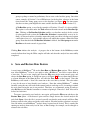
7
The BAMarray Graphical Suite
TM
The graphical suite becomes available once the Gibbs sampler is finished. BAMarrayTM graphics
can be broadly grouped into two categories: Data Plots and Inferential Plots.
1. Data Plots are used to verify the assumption of equal variances. These include (i) cluster
diagnostic plots, (ii) standard deviation plots, (iii) group mean plots, and (iv) running
median plots. The last three plots are based on the transformed data obtained from the
variance stabilization (clustering) step. All data plots are accessible by going to the main
console, clicking on Graph and then clicking on the submenu Data.
2. Inferential Plots are based on estimated parameters from the model and are used for
detecting differentially expressing genes. These include color enhanced shrinkage plots
of Zcut values for identifying differentially expressing genes for a specific group. Also
provided are multigroup Zcut scatter plots for visualizing differentially expressing genes
simultaneously over two or more groups. Shrinkage and Zcut scatter plots are accessible
by going to the main console and clicking on Graph.
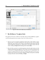
7.1
7.1
Data Plots for Assessing Model Assumptions
31
Data Plots for Assessing Model Assumptions
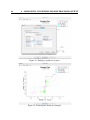
BAMarrayTM provides a cluster diagnostic plot for assessing the adequacy of the variance stabilization transformation. Figure 21 shows such a plot obtained under an Equal variance setting.
The solid blue line represents the percentiles for the theoretical target under a constant variance
assumption. The dashed lines are values under the attempted transformations. As the number
of clusters increases, the dashed lines will become closer to the solid line. See [10] for more
details. Cluster diagnostic plots are also provided under an Unequal variance setting. Only a
theoretical null and the line corresponding to the overall fit are provided in this case.
Figure 21: Cluster plot used for assessing adequacy of variance stabilization transformation.
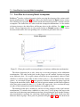
The cluster diagnostic plot is only a first step to assessing adequacy of the stabilization
transformation. Two other useful plots for this purpose are the standard deviation and group
mean difference plots. If an equal variance model has been approximately achieved, there
should be no obvious trend visible in either of these plots (i.e., they should look like random
scatter). As an example, Figure 22 shows genewise standard deviations for groups Aged and
Young on the transformed scales. Notice the lack of apparent structure and the relative tightness
of the data points around the value (1.0, 1.0) that is the target value. Also, note how the range
of values in the horizontal and vertical directions are roughly the same.
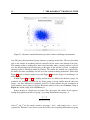
The running median plot is another key tool for assessing adequacy of the equal variance
transformation. If variances have stabilized to values near 1 for all groups (the target value
aimed for in the clustering transformation procedure), then plotting the gene-specific variances
after transformation separately for each group should produce values near 1 with very little
difference between groups. These plots are generated in Figures 23 and 24 for the brain tissue
32
7
THE BAMARRAYTM GRAPHICAL SUITE
Figure 22: Genewise standard deviations plot after variance stabilizing transformation.
data. The plots show transformed group variances as running median lines. The two plots differ
only in the amount of smoothing allowed (controlled by the meter at the bottom of the plot).
The running median is nothing more than a local smoother where a moving window is passed
over the data starting from left and moving to the right. As the window is passed, a continuous
running median is calculated within the window. The smaller the window size (controlled by
the meter), the more variabilility one will see in the estimated running median line. Notice how
Figure 23 tends to bounce around more than Figure 24 where the degree of smoothing is set
much higher.
In both Figures 23 and 24 the running median lines are different for the three groups. In
particular, the standard deviations for the Young group is clearly smaller than the other two
groups. Are these differences significant, and if so, do they indicate that our assumption of
equal variances across groups is suspect? Recall our analysis is based on a Variance setting of
Equal (the default setting used in BAMarrayTM ).
It turns out there is a simple way to test this. For a given gene, the relative error in approximating the population variance for group i by pooling information from group j is
σ
bi2 − σ
bj2
,
4b
σj2 (ni /nj + 1)
where σ
bi2 and σ
bj2 are the sample variances for groups i and j, with sample sizes ni and nj ,
respectively. Therefore, if we want to ensure the relative error of pooling information for group
7.1
Data Plots for Assessing Model Assumptions
Figure 23: Running median plot for group variances - low smoothing.
Figure 24: Running median plot for group variance - high smoothing.
33
34
7
THE BAMARRAYTM GRAPHICAL SUITE
i across groups is less than some value 0 < α < 1, we should check that
|b
σi2 − σ
bj2 |
max
< α.
j
4b
σj2 (ni /nj + 1)
(1)
Similarly, we should check (1) for each group i. For convenience these values are provided
as part of the legend in a running median plot. If we refer to Figure 23 (or Figure 24) we see
that (1) for the Aged, Middle, and Young groups are 0.01, 0.01, and 0.02. These values, and our
previous plots, all suggest the Variance setting of Equal is quite reasonable in this example.
7.2
More On Assuming Equal Variances Across Groups
The following example illustrates a dataset where the assumption of equal variances across
groups is highly suspect. The data considered is based on 12,488 genes and 5 distinct phenotypes (groups). The sample sizes were fairly small in this example (most groups had 3 or 4
observations). Because of this, the choice for the Variance setting plays a big role in the list of
genes found significant. Users should look over this example very carefully if they too find they
are working with an array data set with small numbers of observations within groups.
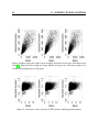
The data was analyzed using both an Equal and Unequal setting for Variance. The running
median plots from the analyses are given in Figures 25 and 26, respectively. Relative errors
calculated using (1) are substantially better for the Unequal variance case, but in some cases
are still relatively high (groups “WT” and “Y122X” have values 0.04 and 0.05, respectively).
In fact, a careful analysis of the standard deviation plots by group (available by clicking
Graph and then Data) shows a characteristic smearing pattern indicating that our variance
clustering algorithm was not able to achieve a constant variance (see Figure 27). Given that we
are already using the more flexible Unequal variance setting, we must conclude the problem
is with the clustering procedure in that not enough clusters are being formed to properly stabilize the data. A simple remedy is to set the number of clusters manually to a relatively large
number. For our example, we found setting the number of clusters at 25 worked well. This
was accomplished by clicking on the Automatic box under Clustering on the main console
and then typing in the number 25 beside the box labelled Manual. Figure 28 shows the new
transformation to much more effective.
7.3
Inferential Plots for Detecting Differentially Expressing Genes
In Section 2.4 we introduced shrinkage plots as a way for identifying outliers, and in Section 2.6
we discussed their use as a way of testing for informative censoring. These two very different
types of problems show the versatility and flexibility of the method. In fact, shrinkage plots were
originally introduced in [1, 2] for a very different purpose: namely as a method for identifying
genes found to be differentially expressing (either up or down) relative to the baseline.
Figure 29 is a example of how a shrinkage plot is used for finding differentially expressing
genes (for many users this will likely be the most appropriate use for these plots). The figure
gives the shrinkage plot for the Zcut gene differential effects of the Age group from the brain
7.3
Inferential Plots for Detecting Differentially Expressing Genes
Figure 25: Running median plot assuming equal variances.
Figure 26: Running median plot assuming unequal variances.
35
36
7
THE BAMARRAYTM GRAPHICAL SUITE
Figure 27: Genewise standard deviations plot after variance stabilizing transformation using
unequal variance setting. Note the “smearing” pattern.
Figure 28: Running median plot obtained under unequal variance setting with number of clusters manually set at a relatively high value.
7.3
Inferential Plots for Detecting Differentially Expressing Genes
37
tissue data (relative to the baseline group, Young). Green points indicate genes which are being
turned off for the Aged group, whereas red indicates genes being turned on. Blue points are
genes that are not differentially expressing.
Figure 29: Shrinkage plot for determining genes differentially expressing for “Aged” group
relative to the baseline group “Young”.
The horizontal axis for the shrinkage plot are Zcut gene differential effects while the vertical
axis are the corresponding posterior variances. Theoretical arguments show that genes that are
truly differentially expressing will have posterior variances that coalesce to 1 on the far left
and right sides of the plot. As the number of samples increases, eventually all of the truly
differentially expressing genes will be found and none of the non-differentially expressing genes
will be falsely detected [2]. BAMarrayTM uses this principle to determine a data adaptive cutoff
value.
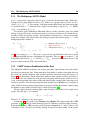
Figure 31 presents a Zcut multigroup scatter plot. This is another powerful graphical tool
for identifying differentially expressing genes (in fact, recall we have already seen an example
of its usefulness in the colon cancer analysis of Section 2.1). Figure 30 shows the dialog box
used to generate the plot. The dialog box is used to select which Zcut values are plotted on
the horizontal and vertical axes respectively. In the case of more than three groups the dialog
box expands and includes an Overlay option that allows an additional group’s Zcut values to
be superimposed on the plot. Triangles indicate genes expressing up or down for the overlayed
group (recall Figure 1 where the overlay group was the Duke C’s).
The legend in the top right corner of Figure 31 indicates how each gene is mapped to a
particular pattern type of differential expression across the experimental groups. As in the
shrinkage plot, the actual decision of whether a gene is significant and which group it belongs
38
7
THE BAMARRAYTM GRAPHICAL SUITE
Figure 30: Choosing which Zcut values go on which axes on the multigroup scatter plot.
Figure 31: Multigroup Zcut scatter plot for 3 groups.
7.4
Adding Gene Labels to Plots and Saving Gene Lists
39
to is done automatically by BAMarrayTM . Different colors correspond to different expression
profile types across groups. A gene could, for example, be significantly upregulated going from
Young to Middle to Aged or down regulated going from Midde to Aged but not from Young to
Middle. These patterns would correspond to the magenta color in the upper right hand quadrant
of Figure 31 and the green data points hugging the negative vertical axis respectively.
Multigroup scatter plots are typically dense. It is often useful to zoom in on particular
genes or particular gene expression patterns to improve clarity. Figure 32 shows the lassoing
zoom-in feature available in BAMarrayTM . A lassoed box focused on only those genes that are
significantly upregulated for the Aged group but not the Middle aged group is illustrated.
The lasso feature is activated by clicking and dragging the mouse cursor over a region of
interest. Releasing the mouse button causes the plot to zoom in (see Figure 33). The user can
repeatedly zoom in, even examining a single gene of interest if they choose. The original plot
can always be restored by clicking the Reset Zoom button at the bottom of the plot. In addition,
the user can move forward or backward (similar to using a web browser) through various levels
of zooming by using the Back and Forward buttons at the bottom of the plot. Lassoing is
available on all data and inferential plots.
7.4
Adding Gene Labels to Plots and Saving Gene Lists
Gene labels can be toggled on or off on almost all BAMararyTM plots. To toggle labels, pull
down the View menu item on the plot and click on the the desired gene subgroup. See Figure 34. Figure 35 shows the labels added to our previously lassoed region. To overlay different
subgroups, simply repeat the process by clicking on a new subgroup. A word of caution: if the
zoom is reset, or the back and forward buttons selected, the user moves through the plots as
desired, but labels will still be on. Gene labels for a particular subgroup can, however, alway be
removed by clicking the appropriate subgroup under the View menu.
Labeled, or unlabelled, genes can be saved as genes lists and output to a text file by pulling
down the File menu on the plot and clicking Save Genes As... (see Figure 36). To add more
genes to a previously saved list simply use the Append Genes feature on the same menu column. For convenience BAMarrayTM makes sure that appended lists of genes contain no duplicate
gene labels. There is also a feature that allows the user to save all significant genes. This is found
on the main console under the File Menu as Save Sig Genes....
7.5
Plotting Options and Using the Gene Tracking Facility
BAMarrayTM plots can be customized by pulling down the Tools menu item on any graph. This
will highlight an Options command which when activated, will open up a Plot Options window
that highlights Preferences (see Figure 37). Plotting label and character sizes can be adjusted
here. Clicking the Apply button activates the desired changes. The default plotting label size is
12 pt and the default plotting character size is 6 pt.
Highlighting the Tracking button in the Plot Options window (Figure 38) opens up a dialog
box that allows the user to manually enter gene labels. Genes can be tagged one at a time by
40
7
THE BAMARRAYTM GRAPHICAL SUITE
Figure 32: Previous figure with lassoing feature activated.
Figure 33: Points captured using lassoing feature.
7.5
Plotting Options and Using the Gene Tracking Facility
41
Figure 34: How to add gene labels.
sequentially entering gene names and then clicking the Add button. The gene list of interest
will then be updated and viewable in the display box below. Genes can be deleted from this list
by highlighting those genes using the mouse and then clicking Remove.
A perhaps more efficient way of using the tracking feature, is to open an entire list of particularly interesting genes. These could for instance map to biological pathways under study.
There are a number of different ways to accomplish this. Regardless of how the tracked gene
list file is created, it must follow the same formatting guidelines as a typical BAMarrayTM data
file as discussed in Section 4. One option is to simply reload the original data file and choose
probesets of interest. This is what is depicted in Figure 38, where 3 genes of interest have been
flagged from the original data file. Note that the gene ID’s are alphabetically ordered automatically by BAMarrayTM . Another option is to save gene lists of interest as described previously,
and then use these gene lists (which will automatically be correctly formatted) to track genes.
This was the strategy employed in the time course profiling example of Section 2.5. The third
option would be to literally create a new file containing only those genes of interest and read
these into the tracking facility.
Once a gene list has been produced, clicking Apply will cause all open plots to have genes
42
7
THE BAMARRAYTM GRAPHICAL SUITE
Figure 35: Gene labels are added to the plot.
Figure 36: Saving labeled genes to an output file.
7.6
Rank Ordering Gene Effects
43
Figure 37: How to change the plotting option preferences.
in the gene list highlighted in boldface and their points enclosed in a dark circle (see Figure 39
for example). We find it handy sometimes to increase the plotting label size in order to clearly
see the highlighted genes on all plots.
7.6
Rank Ordering Gene Effects
A ranked list of genes can be produced using the shrinkage plot in combination with the lasso.
Genes that are highly likely to be differentially expressing will have large Zcut values and
posterior variances near 1. These are the values coalescing to 1 horizontally on the left and
right sides of the shrinkage plot (recall Figure 29). BAMarrayTM adaptively estimates the genes
that are differentially expressing, but the user can always choose a subset of these by lassoing
those with especially large Zcut values. The list can then be saved as a text file as just discussed.
This list can be ranked by the absolute Zcut value. The larger the value, the more likely the gene
is to be differentially expressing.
8
Some Useful Suggestions for Post-Processing Output
Saved output files contain a wealth of information (the information saved depends upon the plot
used to generate it). Files created from shrinkage plots for example contain gene ID’s, Zcut
gene effect values, posterior variances, and a flag identifying whether the gene is differentially
expressing or not; one flag for each group (values are 0, −1, +1 for no differential expression,
44
8
SOME USEFUL SUGGESTIONS FOR POST-PROCESSING OUTPUT
Figure 38: Tracking a specific set of genes.
Figure 39: Tracked genes shown on scatterplot.
45
down-regulated and up-regulated, respectively). Given that these are simple text files, they
can be easily read into other software where further analyses could be done. An example of
this was already presented in Section 2.3 for the invariant set normalization using Batch Mode
processing. More details on Batch Mode processing are given in the Appendix.
In addition to the information contained in BAMarrayTM output files, other sources of information on genes (such as annotation information or PCR validation) could be merged with these
files. We have found it useful for example to import BAMarrayTM gene list files into EXCEL and
color code text to match group membership as identified by the flags. This color coding makes
it simple to track annotation information for example to differential expression pattern type and
look for things like enrichment of detected pathways.
9
Appendix: Batch Mode Processing
BAMarrayTM will support invocation on the command line. This mode of operation will not
present the GUI to the user. The command invocation of BAMarrayTM in batch mode is as
follows:
java [-options] edu.cwru.bam.console.Main [args...]
A sample command invocation of BAMarrayTM is located in USERHOME/BAMarray/bam.batch.sh.
A sample batch file is located in USERHOME/BAMarray/input/batch.xml.
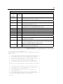
The batch mode protocol is defined in the tables below.
type
Xms<size>
Xmx<size>
D<name>=<value>
Classpath <...>
-b <value>
Option
description and value
Recommended initial Java heap <size> = <32m>
Recommended maximum Java heap <size> = <512m>
System property <name> = <java.library.path>
System property <value> = <./lib/native>
./lib/bam.jar;
./lib/sgt.jar;
./lib/ezlicrun20.jar;
./lib/xml-apis.jar;
./lib/xercesImpl.jar;
./lib/poi.jar;
./lib/commons-cli.jar
./
<value> = XML batch file name
46
9
APPENDIX: BATCH MODE PROCESSING
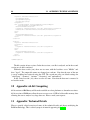
XML DTD Specifications
<?xml encoding=”UTF-8”?>
<!ELEMENT BAMarrayBatch (traceFile?, session+)>
<!ELEMENT traceFile EMPTY>
<!ATTLIST traceFile name CDATA #REQUIRED>
<!ELEMENT session (inputFile, run+)>
<!ELEMENT inputFile (group*)>
<!ATTLIST inputFile name CDATA #REQUIRED>
<!ELEMENT group (#PCDATA)>
<!ELEMENT run (baseline?, outputFile, runStateFile?)>
<!ATTLIST run colorUpreg (Red|Green) ”Red”>
<!ATTLIST run accuracy (Low|Medium|High|Super) ”Medium”>
<!ATTLIST run variance (Equal|Unequal) ”Equal”>
<!ATTLIST run clustering CDATA ”Auto”>
<!ATTLIST run randomSeed CDATA ”Auto”>
<!ELEMENT baseline (#PCDATA)>
<!ELEMENT outputFile EMPTY>
<!ATTLIST outputFile name CDATA #REQUIRED>
<!ATTLIST outputFile genes (Sig|All) ”Sig”> <!ELEMENT runStateFile EMPTY>
<!ATTLIST runStateFile name CDATA #REQUIRED>
47
Element
or
Attribute
traceFile
Required
(Y/N)
session
inputFile
Y
Y
group
N
run
colorUpreg
accuracy
variance
clustering
randomSeed
baseline
Y
N
N
N
N
N
N
outputFile
Y
runStateFile
N
N
XML DTD Verbose Explanations
Default Value or Description
Unspecified -> Output is directed to the application’s default log
file. The file name must end with .log
Each batch file must contain at least one session.
Each session must contain one and only one input file. The file
name must end with .txt or .xls
Unspecified -> All groups are read for the session. Multiple
groups may be also be specified for the session.
Each session must contain at least one run.
Red
Medium
Equal
Auto -> automatic, 1 - 99 -> manual
Auto -> automatic, 1 - 9999 -> manual
Unspecified -> No baseline option is selected. Otherwise a valid
group must be specified.
Each run must contain one and only one output file. This file will
contain all significant genes produced by the run. File name must
end in .txt. Default output is Sig genes only.
The state of each run may be saved for later retrieval via the GUI.
The file name must end with .bam
The sample batch file located in USERHOME/BAMarray/input/batch.xml is listed below:
<?xml version="1.0" encoding="UTF-8"?>
<!DOCTYPE BAMarrayBatch SYSTEM "../security/BAMarray.batch.dtd">
<BAMarrayBatch>







<!-<licenseInfo file="filename.xml" user="username"></licenseInfo>
-->

-->
-->
-->
-->
-->
-->
48
11
APPENDIX: TECHNICAL DETAILS
<inputFile name="brainTissue.txt">
<group>Aged</group>
<group>Middle</group>
<group>Young</group>
</inputFile>
<run colorUpreg="Red" accuracy="Medium" variance="Equal"
clustering="Auto" randomSeed="9999">
<baseline>Middle</baseline>
<outputFile name="brainTissue.out1.txt" genes="Sig"></outputFile>
<runStateFile name="brainTissue.run1.bam"></runStateFile>
</run>
<run>
<baseline>Aged</baseline>
<outputFile name="brainTissue.out2.txt" genes="All"></outputFile>
</run>
</session>
<session>
<inputFile name="brainTissue.xls">
</inputFile>
<run>
<outputFile name="brainTissue.out3.txt"></outputFile>
</run>
<run>
<baseline>Middle</baseline>
<outputFile name="brainTissue.out4.txt"></outputFile>
</run>
</session>
</BAMarrayBatch>
The file consists of two sessions. In the first session, a .txt file is analyzed, and in the second
session an .xls file is analyzed.
Within the first session (.txt), there are two runs, with the baselines set to ”Middle” and
then ”Aged”. The output file names are changed on each run. Note that the state of the run
is saved enabling later retrieval using the GUI. The second run relies on default settings for
”colorUpreg”, ”accuracy”, ”variance”, ”clustering”, and ”randomSeed”.
In the second session (.xls), there are also two runs. Note that the first run is executed is
no-baseline-mode.
10
Appendix: 64-bit Computing
64-bit versions of BAMarray will be made available on select platforms as demand necessitates.
64-bit versions of BAMarray allow the user to access over 4.3GB of addressable memory, thus
allowing the user to analyze very large data sets. Please e-mail your requests.
11
Appendix: Technical Details
Here we provide a brief overview of some of the technical details and theory underlying the
BAM methodology. This is a brief synopsis of material appearing in [1, 2, 3].
11.1
11.1
The Multigroup ANOVA Model
49
The Multigroup ANOVA Model
Let Yi,j represent the expression value for gene j from the ith microarray chip. Each chip i
belongs to some group which we label as k(i). If there are g-groups, then k(i) takes one of gvalues: k(i) ∈ {1, . . . , g}. For example, in the hippocampal brain tissue data, microarray chips
are collected from g = 3 different tissue samples corresponding to Aged (k(i) = 1), Middle
(k(i) = 2) and Young (k(i) = 3).
To search for genes exhibiting a differential effect we define a baseline group over which
change in expression levels are measured against (as discussed earlier we can extend this approach to handle no baseline designs). For notational convenience let g denote the baseline
group (for example, for the brain tissue data, Young represents the baseline group, g = 3). The
multigroup model is defined as:
Yi,j = θj
+βk(i),j
+εi,j ,
i = 1, . . . , n, j = 1, . . . , P.
−→
−→
−→
Baseline effect for gene j
Differential effect
2
)
Independent error, εi,j ∼ Di,j (0, σk(i),j
(2)
In (2), it is assumed βg,j = 0. This way θj represents the overall baseline effect due to group
g. In applying BAM we take a distribution free approach. Thus, in (2), it is assumed εi,j are
2
independent such that E(εi,j ) = 0 and E(ε2i,j ) = σk(i),j
. In essence, the method only uses the
first two sample moments of the data for inference.
11.2
CART Variance Stabilization of the Data
The multigroup ANOVA model does not assume genes have equal variances since this will be
unrealistic for microarray data. Often microarray data exhibit a complex relationship between
the mean and standard deviation, with standard deviations often increasing with means (see
Figure 40 for illustration). On the other hand, while an equal variance model is unrealistic, a
model which has one variance for each gene and each group will lack power. What we need is
a way to group variances into clusters with each cluster having a unique value, but using as few
clusters as possible. The clustering-transformation method used in BAMarrayTM is designed to
strike a balance between using enough clusters to properly stabilize the variance, while keeping
the number of genes within a cluster large to ensure good power [10].
We first explain how the method applies when variances are assumed to be equal across
groups. For each gene j, it is assumed
2
2
= σj2 .
σ1,j
= · · · = σg,j
(3)
However, σj2 is allowed to vary across genes.
Assumption (3) corresponds to the Variance setting Equal. This option invokes the CART
procedure of [10] which sets about clustering genes by similarity of pooled sample variances.
Each instance of the CART procedure yields a cluster configuration, C , with C clusters. For
each cluster l of C , the data is rescaled by dividing all expression values within l by the square
50
11
APPENDIX: TECHNICAL DETAILS
Figure 40: Mean expression values versus standard deviation for each gene from brain tissue
data [16]. Plots from left to right are Young, Middle and Aged rats. Note how variances are
clearly non-homogeneous in each group.
Figure 41: Same plot as above, but after CART variance stabilizing transformation.
11.2
CART Variance Stabilization of the Data
51
root of the mean pooled sample variance. If Jl are the indices for genes in cluster l, the mean
pooled sample variance for cluster l is defined by
σ
b2 (l) =
1 X 2
σ
b ,
Pl j∈J j
l
where Pl is the number of genes in l. Here σ
bj2 is the pooled sample variance for gene j,
g
σ
bj2
X
1
2
=
(nk − 1)b
σk,j
,
(n − g) k=1
where nk is the sample size for group k and
2
σ
bk,j
=
X
1
(Yi,j − Y k,j )2
(nk − 1)
{i:Gi =k}
is the sample variance for gene j from group k.
Note, importantly, that because observations within a cluster is scaled by the same value,
all expression values for a gene j are multiplied by the same value, independent of their group
membership. Therefore, the transformation used by the CART procedure will not affect the
signal to noise ratio for a gene when testing for a differential effect. This is an important
property not shared by other variance stabilizing methods.
The CART transformation is also designed so that if the number of clusters in C equals the
number of genes (C = P ), then the transformed σ
bj2 will satisfy σ
bj2 = 1 for each j. But this
will overfit the data. Even if an equal variance model is true, we still expect variability in the
transformed σ
bj2 around the value of 1. Therefore, rather than choosing a large value of C, and
potentially over-regularizing the problem, with a subsequent loss in power, the prefered method
is to start from C = 1, in which all genes are assumed to have the same variance, and then
gradually increase the value of C until an equal variance model is justified.
BAMarrayTM uses a distance measure approach to determine which value of C to stop at.
The empirical distribution function for the transformed σ
bj is compared to a theoretical distribution function obtained under the null hypothesis and the value of C that leads to the best
fit is chosen. This is all done automatically for the user and typically the user should not be
worried about these details. However, if there are concerns, the Cluster Diagnostic plot (recall
Figure 21) provided in the graphical suite is specifically designed to asses the effectiveness of
the transformation. As C increases, the dashed lines should get closer to the the thick blue
line on the plot representing the nonparametric null distribution. For more technical details, the
reader should consult [10]. See Figure 41 as illustration of the effectiveness of the method.
So far we have assumed variances may differ across genes but not across experimental
groups. To handle the case when (3) is suspect, BAMarrayTM uses a modified CART procedure.
This procedure is implemented when the Variance option is set to Unequal.
A brief discussion of the algorithm is as follows. One should consult [10] for more details.
Essentially the algorithm works by running the equal variance CART procedure (as above)
52
11
APPENDIX: TECHNICAL DETAILS
separately on each group k, obtaining an optimal cluster configuration Ck∗ . All the group cluster
configurations {Ck∗ : k = 1, . . . , g} are then merged into a more refined cluster configuration
C ∗ and this new configuration is then used to rescale observations using the same method as just
discussed. For example in a two group problem, if ’x’ represents a gene, ’|’ a cluster boundary,
and C1∗ and C2∗ are cluster configurations for group 1 and 2, indicated by the top and bottom
rows of the left-side of the figure below, then the refined cluster C ∗ , formed by merging C1∗ and
C2∗ , is given on the right of the figure:
x
x
x
x
| x
x |
x | x
x
x
=⇒
x
x
x | x
x | x
| x
| x
| x
| x
In general, the new cluster configuration C ∗ will contain more clusters than any of the group
configurations Ck∗ , but in our experience will not be so large that over-regularization occurs.
Remark 2. By definition, note carefully that the resulting CART transformed data, under either
the Equal or Unequal variance setting, will have been transformed so that gene population
2
variances σk,j
should all equal σ02 = 1.
11.3
Rescaled Spike and Slab Models
In (2), each gene has a parameter θj representing a mean effect for the baseline group g. The
value for this parameter is of little scientific interest. We use a dimension reduction step to
remove its effect. This is accomplished by centering the transformed data by the baseline mean
value (group g) and restricting the analysis to groups k 6= g. A rescaling is also employed to
allow the use of a rescaled spike and slab model. Such models were shown in [2, 3] to possess
optimal properties.
Hereafter we use Yi,j to denote the CART transformed data. We center and rescale the
CART transformed data to obtain what we refer to as rescaled data. We denote this data by
∗
∗
)t , where
, . . . , Yn−n
Yj∗ = (Y1,j
g ,j
s
N
∗
Yi,j
=
(Yi,j − Y g,j ).
2
σ
bN
2
Here N = (n − ng )P is the total sample size (after excluding the baseline), σ
bN
is the usual un2
biased estimator for σ0 calculated using all the data, and Y g,j is the CART transformed sample
mean for group g for gene j.
Following the centering and rescaling steps, we convert the multigroup model to a rescaled
spike and slab regression model. Let β j = (β1,j , . . . , βg−1,j )t denote the regression parameters
for gene j. The rescaled spike and slab multigroup model is,
(Yj∗ |β
β j , σ2)
(β
β j |γ)
γ
σ2
∼
∼
∼
∼
N(Xj β j , N σ 2 I),
N(0, Γj )
π(dγ)
µ(dσ 2 ),
j = 1, . . . , P
11.4
Continuous Bimodal Priors
53
where Γj is the diagonal matrix with diagonal entries obtained from γ j = (γ1,j , . . . , γg−1,j )t
and γ = (γ t1 , . . . , γ tP )t is the P (g − 1)-dimensional hypervariance vector. Note that the design
matrix Xj is orthogonal. This plays a key role in computation and theoretical development of
BAM.
11.4
Continuous Bimodal Priors
For γ we use the continuous bimodal priors of [2, 3]. The prior π for γ is induced by the
2
2
following parameterization. Define γk,j by γk,j = Ik,j τk,j
, where Ik,j and τk,j
are parameters
with priors specified according to:
iid
(Ik,j |v0 , wk ) ∼ (1 − wk ) δv0 (·) + wk δ1 (·)
iid
−2
(τk,j
|a1 , a2 ) ∼ Gamma(a1 , a2 )
iid
wk ∼ Uniform[0, 1],
k = 1, . . . , g − 1, j = 1, . . . , P.
The choice for v0 (a small near zero value) and a1 and a2 (the shape and scale parameters for
a gamma density) are selected so γk,j has a continuous bimodal distribution with a spike at v0
and a right continuous tail (see Figure 42). Such a prior allows the posterior to either shrink a
coefficient to zero, or not.
Density
0
4
8
12
18
Hypervariance
24
0.0000 0.0040
(b)
8e−04
0e+00
Density
(a)
0
4
8
12
18
24
Hypervariance
Figure 42: Conditional density for γk,j given wk : (a) wk = 0.01, (b) wk = 0.05. Observe that
only the height of the density changes as wk is varied.
The parameters wk also play a special role. Because wk controls the probability that Ik,j
equals 1, it acts like a complexity parameter controlling the number of genes found differentially
expressed for group k. We use g − 1 complexity parameters, one for each group. It is possible
to use a shared complexity w for all groups but our experience has shown this to be less robust
in multigroup problems. For example, if the expression values for a non-baseline group is
significantly different then measurements from other non-baseline group measurements, then
this can unduly inflate or shrink the overall value for w. Using a unique complexity for each
group is also important when group membership has a natural ordering.
54
11.5
11
APPENDIX: TECHNICAL DETAILS
Regularization: Zcut Values
The posterior mean is easily derived by using conjugacy and the orthogonality of Xj . However,
the dimension reduction step of subtracting Y g,j from gene expression values slightly alters the
interpretation of this value as a gene effect. A simple sample size correction is needed to adjust
things. Define the Zcut value
−1/2
nk
∗
b
βk,j = 1 +
E(βk,j |Y∗ ),
k = 1, . . . , g − 1.
ng
Letting Vk,j = E(νk,j |Y∗ ) where νk,j = γk,j /(γk,j + σ 2 ),
∗
βbk,j
= Vk,j
Y − Y g,j
pk,j
,
σ
bN 1/nk + 1/ng
k = 1, . . . , g − 1,
which, up to the factor Vk,j , is a Z-test statistic from an ANOVA model for comparing the
mean for group k to the mean for group g. The value 0 ≤ Vk,j ≤ 1 is a shrinkage factor. The
closer Vk,j is to zero, the more shrinkage there is, while the closer Vk,j is to one, the closer Zcut
becomes to the frequentist value. One can think of Zcut as a Bayesian test statistic.
∗
One can also view βbk,j
as a solution to a constrained least squares optimization problem in
which Vk,j are related to penalty terms. It can be shown that
)
(
g−1
X
1
−
V
1
k,j 2
∗
∗
||Yj∗ − Xj β j ||2 +
βk,j ,
(4)
(βb1,j
, . . . , βbg−1,j
)t = ∆N × arg min
N
V
k,j
βj
k=1
where ∆N is the (g − 1) × (g − 1) diagonal matrix with entries (1 + nk /ng )−1/2 .
Observe how each βk,j coefficient in (4) is penalized by a unique value (1 − Vk,j )/Vk,j . The
closer Vk,j is to 1, the smaller the penalty, while the closer Vk,j is to zero, the larger the penalty.
It is clear that the more adaptive Vk,j is to the true coefficient value, the more accurate the
Bayes test statistic will be in finding differentially expressing genes. Given that we expect few
gene-group differential effects relative to the total number of effects in the model, an optimal
solution to (4) would naturally be sparse; i.e. we would expect many parameters to be zero and
thus many coefficients to have large penalty terms. In [2] it was shown that rescaled spike and
slab models with continuous bimodal priors exhibit adaptive penalization and that this effect is
especially pronounced in sparse settings such as multigroup array data.
The adaptive shrinkage parameters Vk,j are another way that BAM implements regularization. By using all the data, i.e. borrowing strength across genes, we are able to estimate shrinkage parameters and arrive at test statistics that help to reduce the number of false positives. The
typical Z-test
Y − Y g,j
pk,j
Zk,j =
,
k = 1, . . . , g − 1,
σ
bN 1/nk + 1/ng
which is the least squares solution from an ANOVA model, does not take advantage of shrinkage
and regularization. Another way to see this is to note that the Z-tests for gene j are obtained by
11.6
The Zcut Multigroup Rule
55
solving an optimization problem without any penalization:
1
t
∗
2
(Z1,j , . . . , Zg−1,j ) = ∆N × arg min
||Yj − Xj β j || .
βj N
This lack of regularization leads to high variability and excess false positives which becomes
especially pronounced in multigroup experimental designs. Recall our earlier comparison of
Figure 1 based on Zcut to Figure 2 based on the corresponding Z-test.
11.6
The Zcut Multigroup Rule
Ishwaran and Rao [2] showed because of the special nature of the rescaled spike and slab model
that Zcut is likely to be small when the null assumption of no differential effect is true, while if
the null is false, Zcut should be large. They showed that by considering the value of Zcut and
the corresponding posterior variance on a shrinkage plot, one could identify truly expressing
genes from non-expressors. This is called Zcut Multigroup Rule.
Zcut Multigroup Rule: Classify a gene as differentially expressing if its Zcut
value is large and its posterior variance is close to the value of 1. These are the values on the right and left-sides of the shrinkage plot. Note that BAMarrayTM provides
an automated data-based rule which chooses such genes.
12
Acknowledgements
We thank the various granting agencies for research funds that have made this work possible.
In particular, Hemant Ishwaran was supported by National Science Foundation grants DMS0405675 and DMS-0705037, while Sunil Rao was supported by National Institutes of Health
career grant K25-CA89867 and National Science Foundation grant DMS-0405072. This grant
was also partially supported by CTSC funding from Cleveland Clinic and Case Western Reserve
University.
References
[1] Ishwaran H. and Rao J.S. Detecting differentially expressed genes in microarrays using
Bayesian model selection. J. Amer. Stat. Assoc., 98:438–455, 2003.
[2] Ishwaran H. and Rao J.S. Spike and slab gene selection for multigroup microarray data.
J. Amer. Stat. Assoc., 100:764–780, 2005.
[3] Ishwaran H. and Rao J.S. Spike and slab variable selection: frequentist and Bayesian
strategies. Ann. Statist., 33:730–773, 2005.
56
REFERENCES
[4] Ishwaran H., Rao J.S., and Kogalur U.B. BAMarray: Java software for Bayesian analysis
of variance for microarray data. BMC Bioinformatics, 7:59, 2006.
[5] Schena M., Heller R.A., Theriault T.P., Konrad K., Lachenmeier E., and Davis R.W. Microarrays: biotechnology’s discovery platform for functional genomics. Trends in Biotechnology, 16:301–306, 1998.
[6] Schena M. and Davis R.W. Genes, genomes and chips. In M Schena, editor, DNA Microarrays: A Practical Approach. Oxford University Press, Oxford, 1999.
[7] Brown P. and Botstein D. Exploring the new world of the genome with DNA microarrays.
Nature Genetics, 21:33–37, 1999.
[8] Nguyen D., Arpat A.B., Wang N., and Carroll R.J. DNA microarray experiments: biological and technological aspects. Biometrics, 58:701–717, 2002.
[9] Affymetrix, Santa Clara. GeneChipR Exon Array Design, 2005.
[10] Papana A. and Ishwaran H. CART variance stabilization and regularization for high
throughput genomic data. Bioinformatics, 22(18):2254–2261, 2008.
[11] Su A.I. et al. A gene atlas of the mouse and human protein-encoding transcriptomes. Proc.
Nat. Acad. Science, 101:6062–6067, 2004.
[12] Ishwaran H. and Rao J.S. Clustering gene expression profile data by selective shrinkage.
Stat. Prob. Letters, 78:1490–1497, 2008.
[13] Antonellis K.J. et al. Optimization of an external standard for the normalization of
Affymetrix GeneChipR arrays, 2002. Techical Note.
[14] Rosenwald A. et al. The proliferation gene expression signature is a quantitative integrator
of oncogenic events that predicts survival in mantle cell lymphoma. Cancer Cell, 3:185–
197, 2003.
[15] Alizadeh A.A. et al. Distinct types of diffuse large b-cell lymphoma identified by gene
expression profiling. Nature, 403:503–511, 2000.
[16] Blalock E.M., Chen K.C., Sharrow K., Herman J.P., Porter N.M. Foster T.C., and Landfield P.W.Y. Gene microarrays in hippocampal aging: statistical profiling identifies novel
process correlated with cognitive impairment. J. of Neuroscience, 23:3807–3819, 2003.

Top types

Top brands

Top types

Top brands

Top types

Top brands

Top types

Top brands

Top types

Top brands

Top types

Top brands

Top types

Top brands

Top types

Top brands

Top types

Top brands

Top types

Top brands

Top types

Top brands

Top types

Top brands

Top types

Top brands

Download User`s Manual