Download Drift fence simulator:

Drift fence simulator:
technical specifications
and user manual
Version 1
Are simulated fences enough when studying simulated animals or do we need
simulated traps and site searches?
Contents
1 Introduction
2 Model structure
3 Running models
3.1 Data inputs
3.2 Using the model
4 Data output
4.1 Fence arrangement
4.2 Walk paths
4.3 Tabular data
4.3.1 metadata
4.3.2 fence
4.3.3 movement
4.3.4 params
4.3.5 walk
4.3.6 fenceresult
5 Data manipulation
5.1 Using tabular data in R
5.1.1 Establish connections between R and your data logfile
5.1.2 Loading data
5.1.3 Summarising data
5.1.4 Plotting data
5.1.5 Exporting data from R
Appendices
System requirements
Installation
1 Introduction
2 Model structure
3 Running models
3 Data inputs
The simulation is driven by one parameters file that gives the four primary types of
information:
• simulation, giving the stepdist, maxdist, angles, samples and reps parameters
• output, giving the dir parameter where the results will be written to;
• landscape, giving the bounds (describing either a circular or rectangular
landscape) and projection parameters; and
• fences, giving the layout parameter which names a particular fence
arrangement which is followed by the coordinates of the start and end of each
fence.
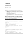
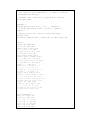
An example of a file that controls the running of a set of simulations is given in the
box below and can be copied to a file called "batchsimulation.sdl" for use. In the
example the fences are arranged in a 5 by 5 grid, with four spacings being simulated
using a series of stepdist, maxdist and angles parameters.
// Trap simulation parameters. Sections can appear in any
order.
simulation {
// stepdist, maxdist and angles parameters can have single or
multiple values
stepdist 1.0 2.0 5.0 10.0
maxdist 10.0 25.0 50.0 100.0 250.0 500.0 1000.0
angles "laplace 0 2" "laplace 0 10" "laplace 0 30" "laplace 0
60" "laplace 0 90" "uniform -180 180"
// samples and reps parameters must each have a single value
// if reps is omitted, default is 1
samples 42525
reps 100
}
output {
// The directory for output database and optional shapefiles.
// Can be overridden by specifying directory and name for one
or more
// output items.
dir "/murray/work/trapsim/testarena"
// root name for walk shapefiles - no output if omitted
walkShapefile "walks"
// root name for fence shapefiles - no output if omitted
fenceShapefile "fences"
// database name - defaults to trapsim.db if omitted
db "trapsim.db"
}
landscape {
bounds type="circle" x=10000 y=10000 radius=1200
// bounds type="rect" x=543000 y=6463000 width=1000
height=1000
// map projection (for codes see http://www.epsgregistry.org/)
projection epsg="20254" // EPSG code for AGD66/Zone 54S
}
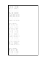
fences {
layout "12.5mgrid" {
9975 9975 9982 9982
9987.5 9975 9994.5 9982
10000 9975 10007 9982
10012.5 9975 10019.5 9982
10025 9975 10032 9982
9975 9987.5 9982 9994.5
9987.5 9987.5 9994.5 9994.5
10000 9987.5 10007 9994.5
10012.5 9987.5 10019.5 9994.5
10025 9987.5 10032 9994.5
9975 10000 9982 10007
9987.5 10000 9994.5 10007
10000 10000 10007 10007
10012.5 10000 10019.5 10007
10025 10000 10032 10007
9975 10012.5 9982 10019.5
9987.5 10012.5 9994.5 10019.5
10000 10012.5 10007 10019.5
10012.5 10012.5 10019.5 10019.5
10025 10012.5 10032 10019.5
9975 10025 9982 10032
9987.5 10025 9994.5 10032
10000 10025 10007 10032
10012.5 10025 10019.5 10032
10025 10025 10032 10032
}
layout "25mgrid" {
9950 9950 9957 9957
9975 9950 9982 9957
10000 9950 10007 9957
10025 9950 10032 9957
10050 9950 10057 9957
9950 9975 9957 9982
9975 9975 9982 9982
10000 9975 10007 9982
10025 9975 10032 9982
10050 9975 10057 9982
9950 10000 9957 10007
9975 10000 9982 10007
10000 10000 10007 10007
10025 10000 10032 10007
10050 10000 10057 10007
9950 10025 9957 10032
9975 10025 9982 10032
10000 10025 10007 10032
10025 10025 10032 10032
10050 10025 10057 10032
9950 10050 9957 10057
9975 10050 9982 10057
10000 10050 10007 10057
10025 10050 10032 10057
10050 10050 10057 10057
}
layout "50mgrid" {
9900 9900 9907 9907
9950 9900 9957 9907
10000 9900 10007 9907
10050 9900 10057 9907
10100 9900 10107 9907
9900 9950 9907 9957
9950 9950 9957 9957
10000 9950 10007 9957
10050 9950 10057 9957
10100 9950 10107 9957
9900 10000 9907 10007
9950 10000 9957 10007
10000 10000 10007 10007
10050 10000 10057 10007
10100 10000 10107 10007
9900 10050 9907 10057
9950 10050 9957 10057
10000 10050 10007 10057
10050 10050 10057 10057
10100 10050 10107 10057
9900 10100 9907 10107
9950 10100 9957 10107
10000 10100 10007 10107
10050 10100 10057 10107
10100 10100 10107 10107
}
layout "100mgrid" {
9800 9800 9807 9807
9900 9800 9907 9807
10000 9800 10007 9807
10100 9800 10107 9807
10200 9800 10207 9807
9800 9900 9807 9907
9900 9900 9907 9907
10000 9900 10007 9907
10100 9900 10107 9907
10200 9900 10207 9907
9800 10000 9807 10007
9900 10000 9907 10007
10000 10000 10007 10007
10100 10000 10107 10007
10200 10000 10207 10007
9800 10100 9807 10107
9900 10100 9907 10107
10000 10100 10007 10107
10100 10100 10107 10107
10200 10100 10207 10107
9800 10200 9807 10207
9900 10200 9907 10207
10000 10200 10007 10207
10100 10200 10107 10207
10200 10200 10207 10207
}
}
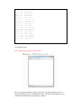
3.2 Using the model
start command and a graphic of the interface
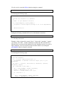
Once you start the modelling software you need to select the parameters file to be
used in the simulations (e.g. batchsimulation.sdl). The file is read and then you can
commence the simulation by pressing the go button.
4 Data output
4.1 Fence arrangement
A description of the fence arrangements is stored in the SQLite database in the fence
table when the simulation is started. Also, shapefiles of the fence configuration in
each layout are written to the working directory. These can then be viewed directly
via a GIS.
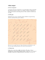
4.2 Walk paths
Walk paths can be stored as a shapefile (warning: simulations can generate large
amounts of walk data if this option is enabled)
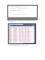
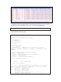
Figure 4.1.1 An example of the fence shape file displayed as the black lines with
some short dispersal paths that miss (red) or hit (green) the drift fences
4.3 Tabular data
Tabular data is exported into a sqlite format database. The tables of data are
metadata, fence, fenceresult, movement, params and walk. They can be extracted
using SQL commands from within the R statistics environment (see section 5.1.2
Loading data into R) and also with the freely available sqlite utility
(http://www.sqlite.org/).
4.3.1 metadata
boundsType
boundsX
boundsY
boundsWidth
boundsHeight
reps
samples
4.3.2 fence
id
layout
fenceID
x0
yo
x1
y1
4.3.3 movement
id
angles
stepdist
maxdist
4.3.4 params
id
fenceLayout
movementId
4.3.5 walk
movementId
walkId
pathDist
offsetDist
offsetDistBearing
4.3.6 fenceresult
paramsId
repId
fenceId
hits
5 Data manipulation
5.1 Using tabular data in R
R is a freely available language and environment for statistical computing and
graphics related to the S statistical package (R Development Core Team (2003). R: A
language and environment for statistical computing. R Foundation for Statistical
Computing, Vienna, Austria. ISBN 3-900051-00- 3, URL http://www.R-project.org ).
Full details are available from the website from where the software and manuals can
be downloaded. Once data is loaded into R you can create your own analyses to
explore the data. Some examples are given below that can be typed in to create these
functions in your R workspace. Otherwise they can be cut and pasted from an
electronic version of this manual. To run these functions you will also require the
RSQLite package which is available from the R website.
In the following sections commands are shown following the R prompt (>) in red
normal text, objects that contain data (dataframes) are red bold italics and objects that
contain command scripts (functions) are blue bold italics.
5.1.1 Establish connections between R and your data output file
To do this you need to be able to connect and disconnect R and your SQlite database
file. For connecting you need to create the db.open function using the command
> fix(db.open)
and entering the following script:
function (filename=NULL, driver=NULL)
{
# Open a database generated for SQLite.
#
# filename - the path and name of the database file; if NULL a
#
dialog will be displayed to choose the file
#
# driver - an optional database driver to manage the connection
if (!require(RSQLite, quietly=TRUE)) {
stop("Can't load the RSQLite package or one of its dependents")
}
if (is.null(filename)) {
tryCatch(
filename <- file.choose(),
error = function(e) {} # dialog cancelled
)
if (is.null(filename)) return( invisible(NULL) )
}
if (!file.exists(filename)) {
cat(paste("Can't find", substitute(filename)))
return(invisible(NULL))
}
if (is.null(driver)) {
driver <- dbDriver("SQLite")
}
con <- dbConnect(driver, filename)
# if (!tmdbValidate(con, show=FALSE)) {
#
dbDisconnect(con)
#
cat(paste(substitute(filename), "is not a valid tm.site
database"))
#
return(invisible(NULL))
# }
s <- dbListTables(con)
if ( length(s) == 0 )
{
print( "Bummer: Either the database can't be opened or it's
empty..." )
return( NULL )
}
print( paste("Tables:", paste(s, collapse=" ")) )
# Return the connection to the database
con <<- invisible( con )
}
You can invoke this function as shown in the following examples, indicating the
command you enter and the response from R which lists the tables it found in your
datafile:
> db.open()
This opens a file selection window and you navigate to your datafile and select it.
The response should look like:
Loading required package: DBI
[1] "Tables: fence fenceresult metadata movement params walk"
or
> db.open("d:/fencesim/results/grid1.db")
[1] "Tables: fence fenceresult metadata movement params walk"
It has created a link (called con) to the datafile file. Once the connection is
established you can issue commands to the database such as the example below.
> dbListTables(con)
[1] "fence" "fenceresult" "metadata" "movement" "params"
[6] "walk"
>
You also need to create the db.close function using the command
> fix(db.close)
and entering the following script:
function ()
{
# Closes the connection to a database
#
# tmdb - an open database connection
if (!require(RSQLite, quietly=TRUE)) {
stop("Can't load the RSQLite package or one of its dependents")
}
dbDisconnect(con)
}
Issuing the following command will now close the database connection.
> db.close()
5.1.2 Loading data into R
Examples of the six data tables created ("fence", "fenceresult", "metadata", "params",
"movement" and "walk") and the command to load them into R are shown below.
The data tables are created in the database file by the simulation and are accessed via
SQL commands. You can load all five tables from the database by creating the
get.datatables function using the command
> fix(get.datatables)
and entering the following script:
function ( )
{
# into the workspace
if ( !( is(con, "SQLiteConnection") ) )
stop("Bummer: no database connection object (con) in your
workspace")
tbl.names <- c("fence", "fenceresult", "metadata", "params",
"movement", "walk")
for ( tablename in tbl.names )
{
qry <- paste("SELECT * FROM", tablename)
result <- dbSendQuery( con, qry )
num.recs <- fetch( result, n=-1 )[1,1]
if ( num.recs > 0 )
{
qry <- paste("SELECT * FROM", tablename)
result <- dbSendQuery( con, qry )
# fetch all records in the result set
x <- fetch( result, n=-1 )
outname <- paste("raw.",tablename, sep = "")
do.call("<<-", list(outname , x ))
# free up memory resources
dbClearResult( result )
}
else
{
warning( paste(tablename, "is empty") )
}
}
}
> get.datatables()
This uses the connection con and loads the fence configuration data into the object
raw.fence in R
and loads the fenceresult into the object raw.fenceresult in R
metadata into the object raw.metadata in R
and loads the movement descriptions into the object raw.movement in R
and loads the layout/movement summary into the object raw.params in R
and loads the sample of walk outcomes for each movement type into the object
raw.walk in R
It is recommended that you use this command when first loading new data into an R
workspace to ensure all the tables of data are loaded and are from the same
simulation.
5.1.3 Summarising data
The following are examples of functions that summarise the various datatables.
To summarise details about the movement types simulated into the walk table you
need to create the summ.walk function
> fix(summ.walk)
and entering the following script:
function()
{
# Assumes datafile raw.walk is loaded
#
col.movementId <- 1
col.walkId <- 2
col.pathDist <- 3
col.offsetDist <- 4
# output data.frame
out <- matrix(0, 0, 12)
colnames(out) <- c("movementId", "angles", "stepdist", "maxdist",
"reps", "min.offset", "lq.offset", "mean.offset", "median.offset",
"uq.offset", "max.offset", "var.offset")
reps <- unique(df.walk[,col.walkId])
nreps <- length(reps)
moves <- unique(df.walk[,col.movementId])
nmoves <- length(moves)
for ( move.num in moves )
{
offset.vec <- rep(0, times=nreps)
for ( i in 1:nreps)
{
offset.vec[i] <- raw.walk[df.walk[, col.walkId] == reps[i] &
raw.walk[,col.movementId] == move.num,col.offsetDist]
}
mean.offset <- mean(offset.vec)
min.offset <- min(offset.vec)
max.offset <- max(offset.vec)
var.offset <- var(offset.vec)
quantiles.offset <- quantile(offset.vec, c(0.25, 0.75))
lq.offset <- quantiles.offset[1]
median.offset <- median(offset.vec)
uq.offset <- quantiles.offset[2]
angle <- raw.movement[raw.movement[,1] == move.num,2]
stepdist <- raw.movement[raw.movement[,1] == move.num,3]
maxdist <- raw.movement[raw.movement[,1] == move.num,4]
out <- rbind(out, matrix( c(move.num, angle, stepdist, maxdist,
nreps, min.offset, lq.offset, mean.offset, median.offset, uq.offset,
max.offset, var.offset), nrow=1, ncol=12 ) )
}
# put the output into the workspace as a data.frame
df.walk.summary <<- as.data.frame( out, stringsAsFactors = FALSE)
}
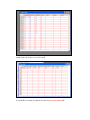
You apply this function to the raw.walk data to generate the df.walk.summary
dataframe by using the following command.
> summ.walk()
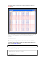
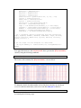
The format of the summary file df.walk.summary is shown below.
To summarise details about the number of fence hits that each layout scores for each
movement style in each replicate you need to create the rep.layout function
> fix(rep.layout)
and entering the following script:
function()
{
# Assumes the raw datafiles are loaded
#
col.paramsId <- 1
col.repId <- 2
col.fenceId <- 3
col.hits <- 4
# output data.frame
out <- matrix(0, 0, 10)
colnames(out) <- c("paramsId", "movementId","fenceLayout",
"angles", "stepdist", "maxdist", "meandist", "mediandist", "rep",
"hits")
reps <- unique(raw.fenceresult[,col.repId])
nreps <- length(reps)
setups <- unique(raw.fenceresult[,col.paramsId])
nsetups <- length(setups)
walkmat <- as.matrix(df.walk.summary)
for ( setup.num in setups )
{
#
hits.vec <- rep(0, times=nreps)
for ( i in 1:nreps)
{
hits <- sum(raw.fenceresult[raw.fenceresult[, col.repId] ==
reps[i] & raw.fenceresult[,col.paramsId] == setup.num,col.hits])
#
mean.hits <- mean(hits.vec)
#
min.hits <- min(hits.vec)
#
max.hits <- max(hits.vec)
#
var.hits <- var(hits.vec)
#
quantiles.hits <- quantile(hits.vec, c(0.25, 0.75))
#
lq.hits <- quantiles.hits[1]
#
#
median.hits <- median(hits.vec)
uq.hits <- quantiles.hits[2]
fenceLayout <- raw.params[setup.num,2]
move.num <- raw.params[setup.num,3]
angle <- raw.movement[raw.movement[,1] == move.num,2]
stepdist <- raw.movement[raw.movement[,1] == move.num,3]
maxdist <- raw.movement[raw.movement[,1] == move.num,4]
meandist <- as.numeric(walkmat[move.num,8])
mediandist <- as.numeric(walkmat[move.num,9])
out <- rbind(out, matrix( c(setup.num, move.num, fenceLayout,
angle, stepdist, maxdist, meandist, mediandist, i, hits), nrow=1,
ncol=10 ) )
}
}
# put the output into the workspace as a data.frame
df.layout.reps <<- as.data.frame( out, stringsAsFactors = FALSE )
}
To summarise details about the number of fence hits that each layout scores for each
movement style you need to create the summ.layout function
> fix(summ.layout)
and entering the following script:
function()
{
# Assumes the raw datafiles are loaded
#
col.paramsId <- 1
col.repId <- 2
col.fenceId <- 3
col.hits <- 4
# output data.frame
out <- matrix(0, 0, 16)
colnames(out) <- c("paramsId", "movementId","fenceLayout",
"angles", "stepdist", "maxdist", "meandist", "mediandist", "reps",
"min.hits", "lq.hits", "mean.hits", "median.hits", "uq.hits",
"max.hits", "var.hits")
reps <- unique(raw.fenceresult[,col.repId])
nreps <- length(reps)
setups <- unique(raw.fenceresult[,col.paramsId])
nsetups <- length(setups)
walkmat <- as.matrix(df.walk.summary)
for ( setup.num in setups )
{
hits.vec <- rep(0, times=nreps)
for ( i in 1:nreps)
{
hits.vec[i] <- sum(raw.fenceresult[raw.fenceresult[, col.repId]
== reps[i] & raw.fenceresult[,col.paramsId] == setup.num,col.hits])
}
mean.hits <- mean(hits.vec)
min.hits <- min(hits.vec)
max.hits <- max(hits.vec)
var.hits <- var(hits.vec)
quantiles.hits <- quantile(hits.vec, c(0.25, 0.75))
lq.hits <- quantiles.hits[1]
median.hits <- median(hits.vec)
uq.hits <- quantiles.hits[2]
fenceLayout <- raw.params[setup.num,2]
move.num <- raw.params[setup.num,3]
angle <- raw.movement[raw.movement[,1] == move.num,2]
stepdist <- raw.movement[raw.movement[,1] == move.num,3]
maxdist <- raw.movement[raw.movement[,1] == move.num,4]
meandist <- as.numeric(walkmat[move.num,8])
mediandist <- as.numeric(walkmat[move.num,9])
out <- rbind(out, matrix( c(setup.num, move.num, fenceLayout,
angle, stepdist, maxdist, meandist, mediandist, nreps, min.hits,
lq.hits, mean.hits, median.hits, uq.hits, max.hits, var.hits),
nrow=1, ncol=16 ) )
}
# put the output into the workspace as a data.frame
df.layout.summary <<- as.data.frame( out, stringsAsFactors =
FALSE)
}
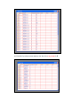
You apply this function to the raw.fenceresult data to generate the df.layout.summary
object by using the following command.
> summ.layout()
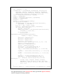
The format of the summary file df.layout.summary is shown below.
To summarise details about the number of fence hits that each fence in each layout
scores for each movement style you need to create the summ.fences function
> fix(summ.fences)
and entering the following script:
function ()
{
out <- matrix(0, 0, 17)
colnames(out) <- c("paramsId", "movementId", "fenceLayout",
"fenceId", "angles", "stepdist", "maxdist", "meandist",
"mediandist", "reps", "min.hits", "lq.hits", "mean.hits",
"median.hits", "uq.hits", "max.hits", "var.hits")
reps <- unique(raw.fenceresult[, "repId"])
nreps <- length(reps)
setups <- unique(raw.fenceresult[, "paramsId"])
nsetups <- length(setups)
fenceId <- -9999
walkmat <- as.matrix(df.walk.summary)
for (setup.num in setups) {
sub.fenceresult <<- raw.fenceresult[raw.fenceresult[,
"paramsId"] == setup.num, ]
hits.vec <- rep(0, times = nreps)
nfences <- unique(sub.fenceresult[, "fenceId"])
for (fence.num in nfences) {
fenceId <- fence.num
subsub.fenceresult <- sub.fenceresult[sub.fenceresult[,
"fenceId"] == fence.num, ]
for (i in 1:nreps) {
hits.vec[i] <sum(subsub.fenceresult[subsub.fenceresult[,
"repId"] == reps[i], "hits"])
}
mean.hits <- mean(hits.vec)
min.hits <- min(hits.vec)
max.hits <- max(hits.vec)
var.hits <- var(hits.vec)
quantiles.hits <- quantile(hits.vec, c(0.25, 0.75))
lq.hits <- quantiles.hits[1]
median.hits <- median(hits.vec)
uq.hits <- quantiles.hits[2]
fenceLayout <- raw.params[setup.num, 2]
move.num <- raw.params[setup.num, 3]
angle <- raw.movement[raw.movement[, 1] == move.num,
2]
stepdist <- raw.movement[raw.movement[, 1] == move.num,
3]
maxdist <- raw.movement[raw.movement[, 1] == move.num,
4]
meandist <- as.numeric(walkmat[move.num, 8])
mediandist <- as.numeric(walkmat[move.num, 9])
out <- rbind(out, matrix(c(setup.num, move.num,
fenceLayout,
fenceId, angle, stepdist, maxdist, meandist,
mediandist, nreps, min.hits, lq.hits, mean.hits,
median.hits, uq.hits, max.hits, var.hits), nrow = 1,
ncol = 17))
}
}
df.fence.summary <<- as.data.frame(out, stringsAsFactors = FALSE)
}
You apply this function to the raw.fenceresult data to generate the df.fence.summary
object by using the following command.
> summ.fences()
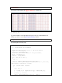
The format of the summary file df.fence.summary is shown below.
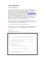
5.1.4 Plotting data
To plot the number of fence hits that each layout scores for each maximum walk
distance you need to create the plot.layout.summary function
> fix(plot.layout.summary)
and entering the following script:
function( )
{
s <- as.matrix(df.layout.summary)
# names and count of fence layouts in df.layout.summary
layouts <- unique(s[,3])
nlayouts <- length(layouts)
# names and count of max offests in df.layout.summary
dists <- unique(s[,6])
ndists <- length(dists)
for ( dist.num in dists )
{
hue <- 0
plot(0, ylim=c(0,max(as.numeric(s[,12]))+10),
xlim=c(0,as.numeric(dist.num)), main=paste("Max dist ", dist.num),
xlab="offset", ylab="hits", col=hue)
for ( layout.num in layouts)
{
hue<- hue + 1
x <- (s[s[, 3] == layout.num & s[,6] == dist.num, 7])
y <- (s[s[, 3] == layout.num & s[,6] == dist.num, 12])
points(x, y, col=hue)
ypos <- max(as.numeric(s[,12]))+10 - (hue*5)
#
legend(0, ypos,layout.num, fill = hue, bty = "n")
}
par(ask=T)
}
You apply this function to the df.layout.summary data to generate the plots by using
the following command.
> plot.layout.summary()
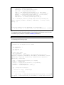
This generates one plot for each maximum walk distance with the x value being the
realised offset and the y value the number of hits, with each fence layout being plotted
in a different colour.
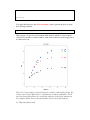
Figure 5.1.4.1 An example of a plot showing the results for walks totalling 100m. The
colours represent four different fence configurations used in the simulations. The X
axis is the mean offset distance for a particular walk type (12 walk type simulated in
this example) and the Y axis is the mean number of fences hit by that walk type
5.1.5 Exporting data from R
At times you may need to use the data in other packages. In the following example the
dataframe df.walk.summary is exported to a file "d:\data\walks.txt" as a comma
delimited file. This can be imported into a spreadsheet for other manipulations.
>write.table(df.walk.summary, file = "c:/data/walks.txt", sep = ",", col.names=TRUE,
row.names=FALSE)
The data can be subdivided in R so that only a subset is exported. There are a variety
of options in the R manual for altering the use of the headings, the data separators etc.
Appendix
Drift fence trapping simulation: compiling and running
The simulation program is written in Java and set up as a Maven project
(http://maven.apache.org/). Once you have Maven installed on your system you
should be able to build the program with the command "mvn clean install" issued
from the top level project directory (the one containing the pom.xml file and this
document). You will need to be connected to the internet when do this so that Maven
can download the libraries required by the program (and the libraries required by
those libraries etc). If this is the first time you have done a Maven build on your
system it is best to kick it off and then go for a long lunch.
The build will create a small program jar file in the target directory. The required
libraries that the program depends on at runtime will have been installed on your
system in your local Maven repository.
To run the program, issue the command "mvn exec:java" from the top level project
directory. You should see a small window open up with buttons to load a parameters
file and run the simulation. See the section 3 of the user manual for more info.
If you want to distribute an executable to other folks without requiring them to have
Maven installed, we recommend you use the Maven Shade plugin to create a single
executable jar containing the program and all required libraries. You will need to hack
your pom.xml file to do this. Don't try to use the Maven Assembly plugin or similar
methods to do this because it won't work properly. If you don't know what any of that
means then you probably don't want to try this. Just relax.
If you want to delve into the code, the guts of the simulation are in the package are
also located at org.cafeanimal.trapsimulation.
Feedback (especially praise and generous offers of funding) can be sent to Michael
Bedward ([email protected]) and Murray Ellis
([email protected]).
Share and enjoy.