1
IMBA Expert™ OCAS/ORAU-Edition (Vers. 4.0)
User Manual
Appendix D: Example Bioassay Cases
August, 2005
Prepared by
Anthony C. James, Ph.D.
ACJ & Associates, Inc.
129 Patton Street
Richland, WA 99352-1618
Tel: (509) 375-7718
FAX: (509) 375-5190
E-mail: [email protected]
Web Site: http://www.acj-associates.com/
© 2001-2005 ACJ & Associates, Inc.
This Appendix provides worked examples of bioassay calculations performed by IMBA Expert™
OCAS/ORAU-Edition. The examples will introduce you to the main "built-in" features and
functions that are provided for bioassay analysis, i.e., for the assessment of intake(s) of
radionuclides based on bioassay measurements.
Contents
D.1. INTRODUCTION ............................................................................................................................... 1
D.2. ESTIMATING A SINGLE INTAKE................................................................................................. 1
D.2.1. INDICATOR NUCLIDE FOR SINGLE INTAKE ...................................................................................... 2
D.2.2. REFERENCE DATE FOR SINGLE INTAKE ........................................................................................... 3
D.2.3. REFERENCE ACTIVITY UNITS FOR SINGLE INTAKE.......................................................................... 4
D.2.4. SELECTING THE REQUIRED MODEL PARAMETERS........................................................................... 4
D.2.5. SELECTING THE INTAKE REGIME (IR1) ........................................................................................... 8
D.2.6. SELECTING WHOLE-BODY AS BIOASSAY QUANTITY ...................................................................... 8
D.2.7. ENTERING THE MEASUREMENT DATA ............................................................................................ 9
D.2.8. GRAPHING THE DATA.................................................................................................................... 10
D.2.9. SELECTING BIOASSAY DATA TO USE - AND CALCULATING INTAKE.............................................. 11
D.2.10. IMPROVING THE DATA FIT .......................................................................................................... 12
D.3. ESTIMATING MULTIPLE INTAKES .......................................................................................... 13
D.3.1. INDICATOR NUCLIDE FOR MULTIPLE INTAKES .............................................................................. 14
D.3.2. REFERENCE DATE FOR MULTIPLE INTAKES .................................................................................. 15
D.3.3. REFERENCE ACTIVITY UNITS FOR MULTIPLE INTAKES ................................................................. 16
D.3.4. SELECTING THE COMMON MODEL PARAMETERS FOR ALL IRS ..................................................... 16
D.3.5. SELECTING THE NUMBER OF INTAKE REGIMES (IRS).................................................................... 20
D.3.6. SELECTING INDEPENDENT MODEL PARAMETERS .......................................................................... 20
D.3.7. DEFINING THE DATE OF EACH INTAKE .......................................................................................... 21
D.3.8. SELECTING THE BIOASSAY QUANTITY .......................................................................................... 21
D.3.9. DATA ENTRY - MULTIPLE INTAKE EXAMPLE ................................................................................ 22
D.3.10. GRAPHING THE DATA - MULTIPLE INTAKES................................................................................ 23
D.3.11. CALCULATING THE INTAKE AMOUNTS ........................................................................................ 24
D.3.12. TESTING THE INTAKE ESTIMATION (EXAMINING THE DATA FIT) ................................................ 26
D.3.13. OPTIMIZING THE INTAKE ESTIMATES .......................................................................................... 27
D.4. USING MULTIPLE BIOASSAY QUANTITIES ........................................................................... 32
D.4.1.
D.4.2.
D.4.3.
D.4.4.
D.4.5.
ERROR ASSUMPTIONS ................................................................................................................... 33
SELECT REFERENCE BIOASSAY MODELS ...................................................................................... 34
HYPOTHETICAL INTAKE SCENARIOS ............................................................................................. 35
REFINING THE INTAKE ASSESSMENT ............................................................................................. 38
EVALUATING THE DOSE ................................................................................................................ 42
D.5. URANIUM ISOTOPIC MIXTURE................................................................................................. 43
D.5.1.
D.5.2.
D.5.3.
D.5.4.
D.5.5.
D.5.6.
D.5.7.
D.5.8.
D.5.9.
SET UP URANIUM MIXTURE .......................................................................................................... 44
ENTER URANIUM-IN-URINE DATA (IN MG/D)................................................................................ 46
ENTER URANIUM-IN-FECES DATA (IN MG/D) ................................................................................ 47
INITIAL JOINT ANALYSIS OF URINE/FECAL DATA ......................................................................... 47
CORRECT FOR DIETARY URANIUM INTAKE ................................................................................... 48
OPTIMIZE INTAKE MODEL PARAMETERS ...................................................................................... 49
COMMITTED DOSES FROM U-MIXTURE......................................................................................... 51
PUBLISHED DATA ON BACKGROUND U-IN-URINE......................................................................... 54
URANIUM EXAMPLE CASE SUMMARY........................................................................................... 54
D.6. ROUTINE TRITIUM URINALYSIS .............................................................................................. 55
D.6.1.
D.6.2.
D.6.3.
D.6.4.
D.6.5.
II
DETERMINE INDIVIDUAL TRITIUM INTAKES AND RESULTING DOSES............................................ 56
SETTING UP THE HTO MODELS .................................................................................................... 56
FITTING DISCRETE HTO INTAKE EVENTS ..................................................................................... 58
CALCULATING DOSES FROM HTO INTAKES .................................................................................. 60
DOSE COMMITTED DURING HTO MONITORING PERIODS ............................................................. 61
IMBA Expert™ OCAS/ORAU-Edition: Example Bioassay Cases
D.6.6. USING THE TRITIUM MONITORING ‘TOOL’.................................................................................... 62
D.6.7. SETTING UP THE TRITIUM ‘TOOL’................................................................................................. 62
D.6.8. LOADING TRITIUM DATA ALREADY IN THE TABLE TOOL ............................................................. 64
D.6.9. LOADING TRITIUM DATA WITH THE ‘IMPORT WIZARD’ ................................................................ 66
D.6.10. AUTOMATED FITTING OF TRITIUM INTAKES ............................................................................... 70
D.6.11. AUTOMATED TRITIUM DOSE CALCULATION ............................................................................... 73
D.6.12. EFFECT OF ASSUMED HTO INTAKE PATTERN ............................................................................. 74
D.6.13. AUTOMATED VS. MANUAL HTO ANALYSIS ................................................................................ 75
D.7.
241
AM LUNG COUNTING (FOR 241PU) ......................................................................................... 79
D.7.1.
D.7.2.
D.7.3.
D.7.4.
D.7.5.
INPUT DATA .................................................................................................................................. 80
ANALYSIS OF 241AM-IN-LUNG DATA – USING ICRP DEFAULTS .................................................... 83
OPTIMIZING HRTM PARAMETER VALUES TO FIT HAN-1 DATA .................................................. 87
IMPROVED REPRESENTATION OF THE HAN-1 DATA ..................................................................... 89
DOSE CALCULATION FOR HAN-1 CASE ........................................................................................ 91
D.8. USING LEAST SQUARES FITTING............................................................................................. 93
D.9. USING BAYESIAN ANALYSIS...................................................................................................... 96
D.9.1.
D.9.2.
D.9.3.
D.9.4.
D.9.5.
PROBABILITY DISTRIBUTION OF INTAKE ASSUMING A UNIFORM PRIOR ....................................... 99
PROBABILITY DISTRIBUTION OF INTAKE ASSUMING AN INVERSE PRIOR..................................... 102
PROBABILITY DISTRIBUTION OF INTAKE ASSUMING A GAUSSIAN PRIOR .................................... 103
PROBABILITY DISTRIBUTION OF INTAKE ASSUMING A LOGNORMAL PRIOR ................................ 105
PROBABILITY DISTRIBUTION OF INTAKE ASSUMING AN ‘ALPHA’ PRIOR .................................... 106
D.10. TRANSDERMAL UPTAKE OF 125I FROM A WOUND.......................................................... 108
D.10.1.
D.10.2.
D.10.3.
D.10.4.
SETTING UP THE ‘WOUND’ INTAKE SCENARIO ......................................................................... 109
TESTING THE ‘DEFAULT’ ASSUMPTION OF ‘RAPID’ UPTAKE ..................................................... 111
DERIVING THE MOST LIKELY ABSORPTION RATES ................................................................... 112
CALCULATING THE POSTERIOR PROBABILITY DISTRIBUTION OF INTAKE.................................. 115
D.11. REFERENCES .............................................................................................................................. 119
IMBA Expert™ OCAS/ORAU-Edition: Example Bioassay Cases
III
This page intentionally left blank.
IV
IMBA Expert™ OCAS/ORAU-Edition: Example Bioassay Cases
D.1. Introduction
The following case examples (taken from real cases) illustrate the main features provided in
IMBA Expert™ OCAS/ORAU-Edition for estimating intake(s) from bioassay data:
•
Calculation of a single intake.
•
Calculation of multiple intakes.
•
Calculation using multiple bioassay data sets.
•
Uranium isotopic mixtures.
•
Routine tritium urinalysis.
•
Am-241 lung counting (for Pu-241).
•
Calculations using Least Squares fitting.
•
Calculations using Bayesian analysis.
•
Transdermal uptake of I-125 from a wound.
D.2. Estimating a Single Intake
This example is one of the study cases taken from IAEA (1999) - see their Annex IV Case 3. The
data are whole-body activity measurements of 60Co commencing 1 day after an accidental
inhalation of a cobalt metal and/or oxide aerosol. All external body surface contamination was
removed by shower-bathing. A profile scan indicated dominant lung deposition. The accident
occurred on February 24th, 1988. The whole-body activity measurements are given in Table D.1.
Table D.1.
60
Co whole-body measurement results.
Measurement date
February 25, 1988
March 1, 1988
March 11, 1988
March 28, 1988
May 16, 1988
August 11, 1988
November 29, 1990
February 19, 1992
Whole-body activity (Bq)
2720
1150
1010
790
482
358
78
35
The following steps (in the listed order) are recommended for calculating the amount of a single
intake (by inhalation) from a set of whole-body measurements - where the time of the intake is
known, and the aerosol and absorption parameters of the inhaled material can be specified with
reasonable confidence. The additional steps required for a more complicated assessment
IMBA Expert™ OCAS/ORAU-Edition: Example Bioassay Cases
1
(involving multiple intakes with unknown parameters) are described in Section D.3.
1. Select the Indicator Nuclide - in the Main Screen.
2. Define the Reference Date - in the Main Screen.
3. Select the Reference Activity Units - in the Main Screen.
4. Select the Bioassay Model and other required Model Parameters - in the Main Screen.
5. Define the Intake Regime (IR1) - in the Main Screen.
6. Select - in the Bioassay Calculations screen - the Bioassay Quantity as "Whole body"
(for display in the top Bioassay Quantity window).
7. Enter the bioassay data - using the data entry "tool" in the Bioassay Quantity window.
8. Graph the bioassay data - using the graph set up "tool" in the Bioassay Quantity
window.
9. Select which bioassay data to use ("Whole body") and click "Start Calculation."
10. Improve the data fit using the Graph of the Bioassay Quantity.
D.2.1. Indicator Nuclide for Single Intake
Figure D.1. Selecting the Indicator Nuclide (60Co).
Select the Indicator Nuclide (60Co in this example case) from the top-right-corner of the Main
Screen (Figure D.1). IMBA Expert™ OCAS/ORAU-Edition will then be able to select
automatically the bioassay model(s) appropriate for cobalt, and automatically take into account
the radioactive half-life of 60Co.
Tip: In this example case, we are using bioassay data to calculate the intake.
Therefore, it is NOT necessary to enter a (hypothetical) value in the displayed
"Intake (IR 1)" dialog box. IMBA Expert™ OCAS/ORAU-Edition will automatically
display the calculated value of Intake in the dialog boxes in both the Main Screen
and Bioassay Calculations screen.
2
IMBA Expert™ OCAS/ORAU-Edition: Example Bioassay Cases
D.2.2. Reference Date for Single Intake
IMBA Expert™ OCAS/ORAU-Edition keeps track of the Intake and all bioassay
measurements on a common timescale. All events are timed with respect to a single Reference
Date (and time-of-day, if necessary). The Reference Date is defined in the Main Screen (Figure
D.2). The IMBA System must always have a reference date - even if you are working entirely in
the Time (d) mode. The default value (January 1st, 1980) is loaded at start-up.
Figure D.2. Default "since" date loaded at start-up.
In this example case, the intake occurred on February 24th, 1988, and so this is the appropriate
value for the Reference Date. The date of the intake is entered directly in the "Time (d) since"
dialog box (Figure D.3). The source data did not give the time-of-day. If no value for the hh:mm
(time-of-day) of the intake is entered, IMBA Expert™ OCAS/ORAU-Edition assigns this as
00:00 (midnight).
Figure D.3. Entering the Reference Date.
Since in this example, the bioassay measurements are tabulated with their collection Date, it is
convenient at this point to switch the "Specify Time As" Units to "Date" (Figure D.4). This
switch from "Time" to "Date" will be passed automatically to the Bioassay Calculations screen
and data tables.
Figure D.4. Switching the Units of Time to Date.
IMBA Expert™ OCAS/ORAU-Edition: Example Bioassay Cases
3
Notice that the "Start Time (d)" value of "0" (Figure D.4) has now automatically switched to
display the "Start Date" as "2/24/1988" - the value entered as the Reference Date before the
switch of time units.
Key Tip: Always set the Reference Date for each case study - in the "Time (d)
since" dialog box ("Units" sub-panel in the Main Screen).
D.2.3. Reference Activity Units for Single Intake
In IMBA Expert™ OCAS/ORAU-Edition, the estimated Intake has the same Unit of activity
as the measured (or predicted) bioassay quantity. As with the Unit of Time, the Unit of
Activity is selected in the Main Screen (Figure D.5). For this example case, the whole-body
activity results are tabulated as Bq. Therefore, the required Unit of Activity is "Bq."
Figure D.5. Selecting the Unit of activity (Intake and Bioassay Quantity) as "Bq."
Warning: IMBA Expert™ OCAS/ORAU-Edition works with the primary bioassay
quantity - which for urinary or fecal excretion is the average excretion rate over a
prescribed collection period (and not the amount of activity in each sample). So,
urinary and fecal bioassay measurements must ALWAYS be entered as the amount
of activity in the sample (in the selected unit) divided by the collection period (in
d).
D.2.4. Selecting the Required Model Parameters
Before you can carry out any calculations with IMBA Expert™ OCAS/ORAU-Edition, you
MUST define all of the necessary Model Parameters. It is most efficient to do this while you are
still in the Main Screen - although (if you forget to do this) it is very easy and quick to switch
backwards and forwards between the Bioassay Calculations screen and the Main Screen (with
a single click).
To estimate an Intake (by inhalation) from a measured Bioassay Quantity, you must define all
the following Model Parameters - as indicated by the "red" buttons in Figure D.6:
4
IMBA Expert™ OCAS/ORAU-Edition: Example Bioassay Cases
•
•
•
•
•
Bioassay model.
Deposition model.
Particle Transport model.
Absorption model.
GI-Tract model.
If you omit defining any of these models, then IMBA Expert™ OCAS/ORAU-Edition will
prompt you for each missing model definition before proceeding with a calculation.
Figure D.6. Bioassay button for selecting the Bioassay Model.
Bioassay model
For the Bioassay model, select the "Standard Co Model" for whole-body retention (Figure D.7):
•
•
•
select "Whole body" as the Bioassay Function - this will already have been defined if
you had previously selected Whole body in the Bioassay Quantity window (Bioassay
Calculations screen);
click the "LOAD ICRP DEFAULTS" button;
click "OK."
Figure D.7. Standard Co Model for Whole body selected as the Bioassay Model.
IMBA Expert™ OCAS/ORAU-Edition: Example Bioassay Cases
5
Deposition model
For the Deposition model, select the "Light worker" (Figure D.8):
•
•
click the "LOAD ICRP DEFAULTS" button;
click "OK."
Figure D.8. Selecting the Deposition Model for a Light worker.
Particle transport model
For the Particle Transport model (Figure D.9):
•
•
click the "LOAD ICRP DEFAULTS" button;
click "OK."
Figure D.9. Selecting the ICRP Default Particle Transport Model.
6
IMBA Expert™ OCAS/ORAU-Edition: Example Bioassay Cases
Absorption model
For the Absorption model, select the Type M ICRP Default model (Figure D.10):
•
•
click the "Type M" button;
click "OK."
Figure D.10. Selecting the Type M Absorption Model.
To select an appropriate (ICRP-recommended) value of f1:
•
•
•
click the "Help" button (Figure D.10);
select the "Abs.: M" row (Figure D.11);
click "OK."
Figure D.11. Selecting the ICRP-recommended value of f1.
GI-Tract model
For the GI-Tract model, select LOAD ICRP DEFAULTS (Figure D.12):
•
•
click the "LOAD ICRP DEFAULTS" button;
click "OK."
IMBA Expert™ OCAS/ORAU-Edition: Example Bioassay Cases
7
Figure D.12. Selecting the ICRP Default GI-Tract Model.
This completes the definition of ALL Model Parameters required to calculate the Intake of
in the IAEA (1999) example case.
60
Co
Key Tip: You can short-cut the process of loading each of the above Model
Parameters individually by clicking the "ICRP Defs LOAD" tool button. You will then
be prompted to choose the Absorption Model and value of f1.
D.2.5. Selecting the Intake Regime (IR1)
By default, IMBA Expert™ OCAS/ORAU-Edition sets up a Single Intake Regime (IR1) - as
an Acute Inhalation (Figure D.13). At this point no value of the Intake has been set (or
calculated).
Figure D.13. IR1 defined (by default) as Acute Inhalation.
D.2.6. Selecting Whole-Body as Bioassay Quantity
The previous steps were carried out in the Main Screen. You select the Bioassay Quantity in
the Bioassay Calculations screen. From the Main Screen you:
•
8
Click the "Bioassay Calculations" button (bottom-right-corner of the Main Screen) - to
open the Bioassay Calculations screen.
IMBA Expert™ OCAS/ORAU-Edition: Example Bioassay Cases
•
In the top Bioassay Quantity window (set as "Table" by default), select "Whole body"
from the drop-down list box (Figure D.14).
This "opens" the first Bioassay Quantity window to display in that window a Table containing
both measured whole-body activity data (on a blue background) and predicted whole-body
activity data (on a green background).
Figure D.14. Drop-down Bioassay Quantity list box.
Note: When it is first opened, the data Table in the Bioassay Quantity window has
only one row. This window is designed to display data values, and NOT for data
entry. Since no data have yet been entered, there are no data to display at this
stage. The "tool" button opens the Table Tool for your selected Bioassay Quantity.
This provides the tools that you will use to enter (and/or edit) the bioassay data – in
the next step.
Tip: Use the scroll bar below the open Bioassay Quantity window to view
additional columns (to the right) that are related to measured bioassay data.
D.2.7. Entering the Measurement Data
IMBA Expert™ OCAS/ORAU-Edition provides a "Table Tool" in the form of an expanded data
table with various editing and automated data entry functions.
Opening the Table Tool
Once you have selected the bioassay quantity for display in the Bioassay Quantity window,
the "tool" button (in the top-right-corner) is activated - see Figure D.15. Click this "tool" button to
open the Table Tool. This will enable you to enter (and/or edit) the whole-body activity data.
Figure D.15. Bioassay Quantity window set to hold "Whole body" data - with active "tool"
button.
IMBA Expert™ OCAS/ORAU-Edition: Example Bioassay Cases
9
“How to use the Table Tool” to enter the data is described in the User Manual (see Section 4.4
under “HOW TO USE THE BIOASSAY CALCULATIONS SCREEN”). For this example, in the
Table Tool, you need to:
1. Enter the eight (paired) values of “Measurement date” and “Whole-body activity (Bq)”
given earlier in Table D.1 (Section D.2) – blue data columns #1 and #3, respectively.
2. Enter “Real” in all eight rows of data column #4 – to signify that these are all real
(reliable) measurements.
3. Enter a (hypothetical) “Uniform Relative” error of “0.1” in all eight rows of data column
#5 – to signify the assumption of a uniform relative error on all measured values.
4. Enter “NORM” in all eight rows of data – to signify that the error in the measured quantity
is assumed to be normally distributed.
The completed Bioassay Quantity table will then be displayed as shown in Figure D.16.
Figure D.16. Table of Bioassay Data for example case of single intake of 60Co.
D.2.8. Graphing the Data
IMBA Expert™ OCAS/ORAU-Edition provides a "Graph Tool" in the form of an expanded
graphical display with full facilities for setting up the type of graph (linear or logarithmic), ordinate
and abscissa scales, etc.
Opening the Graph Tool
Select "Graph" and "Whole body" for display in the second Bioassay Quantity window (Figure
D.17). Then click the "tool" button to open the Graph Tool.
Figure D.17. Opening a Graph window for the Whole body bioassay quantity.
10
IMBA Expert™ OCAS/ORAU-Edition: Example Bioassay Cases
“How to use the Graph Tool” to set up the graph is described the User Manual (see Section 4.5
under “HOW TO USE THE BIOASSAY CALCULATIONS SCREEN”). For this example, in the
Graph Tool, you need to:
1. Click the “Select Axes Automatically” button.
2. In the “Plot” sub-panel, check;
•
•
•
the “Data – Plot” box
the “Data – Error Bars” box
the “Fit – Plot” box.
At this stage, the data and error bars will appear in the Bioassay Quantity graph window as
shown in Figure D.18.
Figure D.18. Graph of Bioassay Data for example case of single intake of 60Co.
Warning: You CANNOT open the Graph Tool until you have entered (or read in
from a file) a value of "Measurement Error" - for every tabulated "Measurement
Value". If you attempt to do this, you will be prompted to complete the data entry.
D.2.9. Selecting Bioassay Data to Use - and Calculating Intake
Before you can calculate the amount of Intake, you MUST first Select which data to use. In the
"CALCULATION" sub-panel (Bioassay to Intake - Figure D.19):
•
check the Whole body box.
If you forget to do this, you will be prompted. To calculate the maximum likelihood estimate of
the Intake amount:
•
click the "Start Calculation" button (Figure D.19).
This will:
•
•
display automatically the Intake amount for the single Intake Regime (IR1);
plot automatically the corresponding fit to the data points (see Figure D.19) - provided
that the "Plot Fit" box was checked in the Graph Tool.
In this example, with the selected values of Model Parameters, the calculated Intake amount is
10,341 Bq.
IMBA Expert™ OCAS/ORAU-Edition: Example Bioassay Cases
11
Figure D.19. Calculated Intake amount with corresponding “best fit“ to the data.
You will see from the Table and Figure displayed in the Bioassay Quantity windows (Figure
D.19) that the fit to data points is generally poorer than the assumed measurement errors. This
fit can be improved quite readily, by reviewing, and if necessary making reasonable changes
to, one or more of the assumed Model Parameters (see the following sub-section).
D.2.10. Improving the Data Fit
In this example case (single intake of 60Co by inhalation), the fit to the data is clearly improved
by varying the assumed aerosol Activity Median Aerodynamic Diameter (AMAD) from the 5-µm
default value recommended by ICRP - to an AMAD of 1 µm (with σg = 2.47). The resulting
improved data fit (at least to the earliest 6 data points) is shown in Figure D.20. The
corresponding (better) estimate of the Intake amount is 9,805 Bq.
Figure D.20. Improved data fit obtained by changing the value of aerosol AMAD.
Tip: As an instructive exercise, try varying other Model Parameters (within
reasonable ranges) to examine their effect on the data fit.
12
IMBA Expert™ OCAS/ORAU-Edition: Example Bioassay Cases
D.3. Estimating Multiple Intakes
This example is taken from Miller et al. (1999) - see their Appendix 2. The data are urinary
excretion measurements of 238Pu in 37 samples taken from March 15th, 1968 through May 28th,
1979. The worker concerned had several intakes (by inhalation) of mixed 239Pu/238Pu:
1. In the mid-1950s - and assumed for analysis purposes to have occurred on June 9th,
1945.
2. On May 8th, 1971.
3. At some unknown time between the routine sampling dates of September 22nd, 1971 and
September 18th, 1972.
In their analysis, Miller et al. assigned the date of the third intake as March 21st, 1972 (mid-way
between the prior- and post-intake samples). No information about the physical properties of the
239
Pu/238Pu material (or aerosol) was presented. The urinalysis results are given in Table D.2.
Table D.2. 238Pu urinalysis results.
Collection date
Excretion rate (mBq d-1) ± 1 SD
March 15, 1968
1 ± 0.9
June 13, 1968
1.8 ± 0.9
September 13, 1968
0.3 ± 0.9
December 13, 1968
4.8 ± 2
March 20, 1969
0 ± 0.9
December 18, 1969
0 ± 0.9
March 19, 1970
0 ± 0.9
June 18, 1970
0.5 ± 0.9
September 24, 1970
0.5 ± 0.9
March 18, 1971
1.2 ± 0.7
June 29, 1971
4.1 ± 0.7
September 22, 1971
2.2 ± 0.5
September 18, 1972
12.9 ± 1.6
December 8, 1972
7.5 ± 1.1
March 15, 1973
2 ± 0.4
June 27, 1973
3 ± 0.6
September 17, 1973
2.7 ± 0.5
December 21, 1973
3.1 ± 0.6
March 21, 1974
1.1 ± 0.4
June 17, 1974
3.8 ± 0.7
September 16, 1974
2.1 ± 0.5
December 18, 1974
1.5 ± 0.4
March 17, 1975
2 ± 0.4
June 16, 1975
1.1 ± 0.4
September 19, 1975
0.8 ± 0.4
December 12, 1975
1 ± 0.4
March 17, 1976
1.2 ± 0.4
July 2, 1976
1.4 ± 0.4
September 12, 1976
1.4 ± 0.4
December 8, 1976
0.5 ± 0.4
June 24, 1977
1 ± 0.4
September 15, 1977
0.4 ± 0.4
September 1, 1978
2.2 ± 0.5
October 20, 1978
0.3 ± 0.4
January 18, 1979
0.9 ± 0.4
April 20, 1979
0.4 ± 0.4
May 28, 1979
1.6 ± 0.4
IMBA Expert™ OCAS/ORAU-Edition: Example Bioassay Cases
13
The following steps (in the listed order) are recommended for making an initial estimate of the
amounts of the three separate intakes in this example.
1.
2.
3.
4.
5.
6.
7.
8.
9.
10.
11.
12.
Select the Indicator Nuclide - in the Main Screen.
Define the Reference Date - in the Main Screen.
Select the Reference Activity Units - in the Main Screen.
Select the Common Model Parameters to be used for all IRs - in the Main Screen.
Select the Number of Intake Regimes (IRs) - in the Main Screen.
Select the option for Independent Model Parameters for all IRs - in the Main Screen.
Define the Date of Each Intake - in the Main Screen.
Select - in the Bioassay Calculations screen - the Bioassay Quantity as "Urine" (for
display in the top Bioassay Quantity window).
Enter the bioassay data - using the data entry "tool" in the Bioassay Quantity window.
Graph the bioassay data - using the graph set up "tool" in Bioassay Quantity window.
Select which bioassay data to use ("Urine") in the CALCULATION sub-panel.
Click the "Start Calculation" button.
When you have completed these steps - and made your initial estimate of the amounts of each
intake - you will start the iterative process of refining these estimates by comparing the
predicted urinary excretion rates with the measured values.
Tip: When you are familiar with the operation of IMBA Expert™ OCAS/ORAUEdition, you will find that the initial Steps 1 through 10 can be performed in any
order (to suit your own working style) - just as long as ALL of the parameter and data
values have been defined BEFORE you click the "Start Calculation" button.
Important: If you have missed a step, IMBA Expert™ OCAS/ORAU-Edition will
prompt you to carry this out - but only if the required data values are missing (null).
Warning: It is your responsibility to check that ALL of the model parameters have
been set to your specific requirements. IMBA Expert™ OCAS/ORAU-Edition will
use whatever values are in memory when you click the "Start Calculation" button.
D.3.1. Indicator Nuclide for Multiple Intakes
Figure D.21. Selecting the Indicator Nuclide (238Pu).
Select the Indicator Nuclide (238Pu in the example case) from the top-right-corner of the Main
Screen (Figure D.21). IMBA Expert™ OCAS/ORAU-Edition will then be able to select
automatically the bioassay model(s) appropriate for plutonium, and automatically take into
account the radioactive half-life of 238Pu.
Tip: In this example case, we are using bioassay data to calculate intake(s).
Therefore, it is NOT necessary to enter a (hypothetical) value in the displayed "Intake
(IR 1)" dialog box. IMBA Expert™ OCAS/ORAU-Edition will automatically display
the calculated values of Intake(s) in their respective dialog boxes.
14
IMBA Expert™ OCAS/ORAU-Edition: Example Bioassay Cases
D.3.2. Reference Date for Multiple Intakes
This is a KEY parameter - especially for cases where more than one intake is being analyzed.
IMBA Expert™ OCAS/ORAU-Edition keeps track of all Intakes and bioassay measurements
on a common timescale. All events are timed with respect to a single Reference Date (and timeof-day, if necessary). The Reference Date is defined in the Main Screen (Figure D.22). The
IMBA System must always have a reference date - even if you are working entirely in the Time
(d) mode - so a default value (January 1st, 1980) is loaded at start-up.
Figure D.22. Default "since" date loaded at start-up.
In this example case, the earliest date of interest is June 9th, 1945, and so this is the appropriate
value for the Reference Date. This is entered directly in the "Time (d) since" dialog box (Figure
D.23).
Figure D.23. Entering the Reference Date.
Since in this example, the bioassay measurements are tabulated with their collection Date, it is
necessary at this point to switch the "Specify Time As" Units to "Date" (Figure D.24). This
switch from "Time" to "Date" will be passed automatically to the Bioassay Calculations screen
and data tables.
Figure D.24. Switching the Units of Time to Date.
IMBA Expert™ OCAS/ORAU-Edition: Example Bioassay Cases
15
Notice that the "Start Time (d)" value of "0" (Figure D.24) has now automatically switched to
display the "Start Date" as "6/9/1945" - the value entered as the Reference Date before the
switch of time units.
Key Tip: Always set the Reference Date for each case study - in the "Time (d)
since" dialog box ("Units" sub-panel in the Main Screen).
D.3.3. Reference Activity Units for Multiple Intakes
In IMBA Expert™ OCAS/ORAU-Edition, the estimated Intake has the same Unit of activity
as the measured (or predicted) bioassay quantity. As with the Unit of Time, the Unit of
Activity is selected in the Main Screen (Figure D.25).
Figure D.25. Selecting the Unit of activity (Intake and Bioassay Quantity) as "Bq."
Warning: IMBA Expert™ OCAS/ORAU-Edition works with the primary bioassay
quantity - which for urinary or fecal excretion is the average excretion rate over a
prescribed collection period (and not the amount of activity in each sample). So,
urinary and fecal bioassay measurements must ALWAYS be entered as the amount
of activity in the sample (in the selected unit) divided by the collection period (in
d).
D.3.4. Selecting the Common Model Parameters for All IRs
Before you can carry out any calculations with IMBA Expert™ OCAS/ORAU-Edition, you
MUST define all of the necessary Model Parameters. It is most efficient to do this while you are
still in the Main Screen - although (if you forget to do this) it is very easy and quick to switch
backwards and forwards between the Bioassay Calculations screen and the Main Screen (with
a single click).
You can "pre-set" ALL model parameters to "ICRP Default" values - with a single
click of the "ICRP DEFS Load" button.
Then, as you open additional Intake Regimes (IRs), the "Default"
models will be loaded automatically - so that you won't have to carry out all of the
individual steps listed below (for each IR). In general, it is much quicker to load (first)
ALL ICRP Default model parameter values (for ALL IRs) - and then change only the
relatively few parameters values that are specific to your case.
16
IMBA Expert™ OCAS/ORAU-Edition: Example Bioassay Cases
To estimate an Intake (by inhalation) from a measured Bioassay Quantity, you must define all
the following Model Parameters - as indicated by the "red" buttons in Figure D.26:
•
•
•
•
•
Bioassay model.
Deposition model.
Particle Transport model.
Absorption model.
GI-Tract model.
If you omit defining any of these models, then IMBA Expert™ OCAS/ORAU-Edition will
prompt you for each missing model definition before proceeding with a calculation.
Figure D.26. Bioassay button for selecting the Bioassay Model.
Bioassay model
For the Bioassay model, select the "Standard Pu Model" for urinary excretion (Figure D.27):
•
•
•
select "Urine" as the Bioassay Function - this will already have been defined if you had
previously selected Urine in the Bioassay Quantity window (Bioassay Calculations
screen);
click the "LOAD ICRP DEFAULTS" button;
click "OK."
Figure D.27. Standard Pu Model for Urine selected as the Bioassay Model.
Deposition model
For the Deposition model, select the "Light worker" (Figure D.28):
•
•
click the "LOAD ICRP DEFAULTS" button;
click "OK."
IMBA Expert™ OCAS/ORAU-Edition: Example Bioassay Cases
17
Figure D.28. Selecting the Deposition Model for a Light worker.
Particle transport model
For the Particle Transport model (Figure D.29):
•
•
click the "LOAD ICRP DEFAULTS" button;
click "OK."
Figure D.29. Selecting the ICRP Default Particle Transport Model.
18
IMBA Expert™ OCAS/ORAU-Edition: Example Bioassay Cases
Absorption model
For the Absorption model, select the Type M ICRP Default model (Figure D.30):
•
•
click the "Type M" button;
click "OK."
Figure D.30. Selecting the Type M Absorption Model.
To select an appropriate (ICRP-recommended) value of f1:
•
•
•
click the "Help" button (Figure D.30);
select the "Abs.: M" row (Figure D.31);
click "OK."
Figure D.31. Selecting the ICRP-recommended value of f1.
GI-Tract model
For the GI-Tract model, select LOAD ICRP DEFAULTS (Figure D.32):
•
•
click the "LOAD ICRP DEFAULTS" button;
click "OK."
Figure D.32. Selecting the ICRP Default GI-Tract Model.
IMBA Expert™ OCAS/ORAU-Edition: Example Bioassay Cases
19
This completes the definition of ALL Model Parameters required to calculate the (3) Intakes of
238
Pu in the Miller at al. (1999) example case.
Key Tip: Don't forget that you can short-cut the process of loading each of the
above Model Parameters individually by clicking the "ICRP DEFS LOAD" tool button.
You will then be prompted to choose just the Absorption Model (i.e., type of
absorption behavior) and the value of f1.
D.3.5. Selecting the Number of Intake Regimes (IRs)
Figure D.33. Selecting 3 separate Intake Regimes (IRs).
In the "Intake Scenario" panel ("Intake Regimes" sub-panel) simply enter the required number
of individual (separate) intake events in the dialog box.
D.3.6. Selecting Independent Model Parameters
Figure D.34. Un-checking "Apply Model Params to All IRs" in the "Advanced" menu.
By default, IMBA Expert™ OCAS/ORAU-Edition applies all of the defined Model Parameters
to All Intake Regimes (IRs). If you want to specify independently ANY parameter value (e.g.,
the date/time of the Intake) for ANY individual IR, you MUST first un-check the default condition
in the "Advanced" menu (Figure D.34).
Note: When you have selected more than 1 Intake Regime - AND you have unchecked the default "Apply Model Params to All IRs," the appropriate number of
tabs will appear automatically in the "Model Parameters" sub-panel (Figure D.35).
You can then proceed to set up (or modify) ANY model parameter for ANY
individual IR#.
20
IMBA Expert™ OCAS/ORAU-Edition: Example Bioassay Cases
Figure D.35. Individual IR# tabs for setting up Model Parameters specific to each IR.
D.3.7. Defining the Date of Each Intake
Figure D.36. Setting the Date of IR 2 as May 8th, 1971.
Once you have specified independent model parameters for all IRs, you simply click on each
IR # tab displayed in the "Intake Regimes" sub-panel to specify the intake parameter values for
that IR # (Figure D.36). For the initial estimate of the amounts of each (acute) Intake:
•
•
enter the "Start Date" of IR 2 as May 8th, 1971;
enter the estimated "Start Date" of IR 3 as March 21st, 1972.
Note: In this example, all 3 of the intakes are assumed to be "acute." You can, of
course, specify "chronic" for ANY intake, as appropriate.
D.3.8. Selecting the Bioassay Quantity
Figure D.37. Drop-down Bioassay Quantity list box.
IMBA Expert™ OCAS/ORAU-Edition: Example Bioassay Cases
21
The previous steps were carried out in the Main Screen. You select the Bioassay Quantity in
the Bioassay Calculations screen. From the Main Screen you:
•
•
•
Click the "Bioassay Calculations" button (bottom-right-corner of the Main Screen) - to
open the Bioassay Calculations screen.
Select the "Bioassay to Intake" direction for the CALCULATION (indicated by a blue
arrow) - if you loaded a "new" (blank) Parameter File, this calculation mode will have
been selected already (by default).
In the top Bioassay Quantity window (set as "Table" by default), select "Urine" from the
drop-down list box (Figure D.37).
This "opens" the first Bioassay Quantity window to display in that window a Table containing
both measured urinary excretion data (on a blue background) and predicted urinary excretion
data (on a green background).
Note: When it is first opened, the data Table in the Bioassay Quantity window has
only one row. This window is designed to display data values, and NOT for data
entry. Since no data have yet been entered, there are no data to display at this
stage. The "tool" button opens the Table Tool for your selected Bioassay Quantity.
This provides the tools that you will use to enter (and/or edit) the bioassay data - in
the next step.
Tip: Use the scroll bar below the open Bioassay Quantity window to view
additional columns (to the right) that are related to measured bioassay data.
D.3.9. Data Entry - Multiple Intake Example
IMBA Expert™ OCAS/ORAU-Edition provides a "Table Tool" in the form of an expanded data
table with various editing and automated data entry functions..
Opening the Table Tool
The Table Tool shows all of the data columns (without you having to scroll). When you open this
[from a Bioassay Quantity (BQ) window], the Table Tool will display the same number of rows
as the BQ window. Initially, only a default single row is displayed. Your first task is to open up
enough rows to hold all of the measured bioassay data that you want to analyze - in this
example, 37 values of daily urinary excretion:
•
Enter "37" in the "Number of Rows" dialog box (bottom panel, left-of-center - see Figure
D.38).
•
Click the "Apply" button to the right of the dialog box.
Tip: The number of data rows shown in the Table Tool depends on your screen
resolution setting. The minimum recommended screen resolution (1024 X 768) shows
35 rows - as in Figure D.38.
22
IMBA Expert™ OCAS/ORAU-Edition: Example Bioassay Cases
Table D.38. Table Tool with 37 rows opened.
Note: For a detailed description of “How to Use the Table Tool" – see the User
Manual (Section 4.4 under “HOW TO USE THE BIOASSAY CALCULATIONS
SCREEN”).
D.3.10. Graphing the Data - Multiple Intakes
IMBA Expert™ OCAS/ORAU-Edition provides a "Graph Tool" in the form of an expanded
graphical display with full facilities for setting up the type of graph (linear or logarithmic), ordinate
and abscissa scales, etc.
Opening the Graph Tool
Select "Graph" and "Urine" for display in the second Bioassay Quantity window. Then click the
"tool" button to open the Graph Tool (Figure D.39).
Figure D.39. Opening the Graph Tool for the Urine bioassay quantity.
IMBA Expert™ OCAS/ORAU-Edition: Example Bioassay Cases
23
Note: For a detailed description of “How to Use the Graph Tool" see the User
Manual (Section 4.5 under “HOW TO USE THE BIOASSAY CALCULATIONS
SCREEN”).
D.3.11. Calculating the Intake Amounts
Before you can calculate the amounts of each of the three Intakes, you MUST first Select which
data to use. In the "CALCULATION" sub-panel (Bioassay to Intake - Figure D.40):
•
check the Urine box.
If you forget to do this, you will be prompted.
Figure D.40. Selecting Urine as the Bioassay Quantity to use to estimate the Intakes.
To calculate the maximum likelihood estimate of the Intake amounts:
•
click the "Start Calculation" button (Figure D.40).
This will:
•
•
display automatically the Intake amounts for all three Intake Regimes (IR1, IR2 and
IR3);
plot automatically the corresponding fit to the data points (see Figure D.41) - provided
that the "Plot Fit" box was checked in the Graph Tool.
Figure D.41. Calculated Intakes with corresponding “best fit” to the data (for assumed Type M
absorption behavior).
24
IMBA Expert™ OCAS/ORAU-Edition: Example Bioassay Cases
In this example, with the selected values of Model Parameters, the calculated Intakes are:
•
•
•
IR1 = 0.91 Bq;
IR2 = 398.6 Bq;
IR3 = 381.1 Bq.
Figure D.41 shows that the resulting fit to data points is poor, especially:
1. in not representing the well defined "peak" (from IR3) in the measured urine data (with its
subsequent rapid decay) at 9,963 d;
2. in predicting "zero" urinary excretion (from IR1 = 0) prior to the second intake (from IR2)
th
on May 8 , 1971 (at 9,464 d).
To improve the "fit" to the measured urinary excretion data, it is necessary to review, and modify
appropriately, the assumed Model Parameters for each Intake Regime.
For example, since the absorption behavior of the inhaled material is unknown, it is reasonable
to change this (for all 3 IRs), and see the effect on the data fit. Changing the absorption
behavior for All IRs to "Type S" - with the associated value of f1 = 0.00001 - and recalculating
the intake amounts, gives the result shown in Figure D.42.
Figure D.42. Calculated Intakes with corresponding best fit to the data for assumed Type S
absorption behavior.
Clearly, the assumption of Type S absorption behavior gives a worse overall fit to the measured
urine data than Type M (Figure D.41). Type S behavior does predict a step-wise increase in
urinary excretion at 9,464 d (from IR2), and also the presence of finite excretion prior to that
date (from IR1). However:
1. it CANNOT fit the observed sharp increase in the excretion rate following IR3;
2. NOR the observed sharp drops in the excretion rate following both IR2 and IR3.
Note that changing the assumed absorption behavior also changes significantly the "best
estimates" of the intake amounts to:
•
•
•
IR1 = 8,424 Bq;
IR2 = 6,501 Bq;
IR3 = 0.0005 Bq.
IMBA Expert™ OCAS/ORAU-Edition: Example Bioassay Cases
25
D.3.12. Testing the Intake Estimation (Examining the Data Fit)
Although the assumption of Type M absorption behavior in the “multiple intake” example gave a
better fit (Figure D.41) to the measured data than Type S, the fit was still not good. In order to
improve this, IMBA Expert™ OCAS/ORAU-Edition provides a further powerful tool for
optimizing the data fit. This is the "Intakes to Bioassay" option in the "CALCULATIONS" subpanel. This option enables you to predict the bioassay quantity with sufficient time-resolution
to examine in detail the fit achieved for rapidly changing data (significant observed "peaks" in
the data).
The first step in testing an intake estimation is to switch the "CALCULATION" mode from
"Bioassay to Intake" (blue arrow) to "Intakes to Bioassay" (green arrow) - as shown in Figure
D.43.
Figure D.43. Setting up a series of times at which to predict the bioassay quantity.
In this example, the measured urinary excretion data exhibited significant "peaks" in 1971 and
1972. However, these bioassay data were taken at "routine" sampling intervals - and NOT in
response to intake events (known or suspected). As a result, much of the early urinary
excretion of relatively soluble plutonium would have been missed. The "Intakes to Bioassay"
option enables this predicted early excretion to be examined on the same graph plot as the
measured data.
For this example (Figure D.43):
•
•
•
•
•
•
•
select 200 as the Number of Dates (1-200);
select Linear for the time series;
specify the Start Date as "1/1/71";
specify the Stop Date as "12/31/72";
click the "Send to all open windows →" button;
enter "1" in the "Specify Collection Periods [Col 2]" dialog box;
click the "Send →" button.
This will automatically:
1. open 200 rows (green background) in the Bioassay Quantity table;
2. enter [in Column 1] the 200 values of date/time (at linear intervals);
3. enter "1" for the Collection Period [Column 2] for each of the 200 sample times.
26
IMBA Expert™ OCAS/ORAU-Edition: Example Bioassay Cases
To calculate the predicted amount of urinary excretion for all 200 (hypothetical) samples - for the
displayed "initial" estimates of the intake amounts - and to display the results in Column 3 of
the table:
•
click the "Start Calculation" button.
The predicted values are shown in Figure D.44.
Figure D.44. Predicted bioassay quantity displayed in the Bioassay Quantity window.
Warning: If you are using a slow processor (< 400 MHz), you will have to wait
several minutes for the calculation of 200 excretion values to finish.
Tip: If your processor is too slow, decrease the number of time points.
D.3.13. Optimizing the Intake Estimates
This is done by improving the fit of the predicted bioassay quantity to the bioassay data - using
the Graph Tool (Figure D.45):
•
•
click the "Select Axes Automatically" button ("Tools" sub-panel);
check the "Plot" dialog box under "Bioassay Predictions" ("Plot" sub-panel).
The predicted values of the bioassay quantity will automatically be added to the graph of the
data (as a green curve).
IMBA Expert™ OCAS/ORAU-Edition: Example Bioassay Cases
27
Figure D.45. Adding the "Bioassay Predictions" curve to the data plot.
The predicted bioassay quantity curve is also added automatically to the Bioassay Quantity
window display (Figure D.46).
Figure D.46. Curve of predicted bioassay quantity displayed in Bioassay Quantity window.
Tip: Use the higher resolution provided by the Graph Tool for critical comparisons
of predicted curves with the measured values.
Examine closely the Graph Tool plot (Figure D.45), and you will see that:
1. the predicted early urinary excretion for the known intake time (IR2) is substantially
higher than the next measured value (at 9,516 d);
2. the next two data points (at 9,516 and 9,601 d) are reasonably-well predicted.
3. the values of the two highest measured values (following IR3) are NOT predicted.
28
IMBA Expert™ OCAS/ORAU-Edition: Example Bioassay Cases
Clearly, from the predicted rapid fall-off in urinary excretion, the actual date of intake for IR3
must have been much closer to 9/18/1972 (9,963 d), the date of the next urine sample, than the
"mid-interval" date (3/21/1972) assumed initially for IR3.
To test this interpretation:
•
•
in the Main Screen, change the assumed "Start Date" for IR3 to "9/11/72";
back in the Bioassay Calculations screen, "Bioassay to Intakes" option (blue arrow),
click the "Start Calculation" button.
Figure D.47. Calculating new intake amounts for a different assumed date of intake for IR3.
With the revised date of intake for IR3, the calculated Intakes are:
•
•
•
IR1 = 0 Bq;
IR2 = 355.9 Bq;
IR3 = 367.7 Bq.
Figure D.48 shows the enlarged plot in the Graph Tool.
Figure D.48. Improved data fit obtained by refining the assumed date of intake for IR3.
To plot the corresponding predicted bioassay quantity curve simply:
•
•
switch to the "Intakes to Bioassay" option (green arrow);
click the "Start Calculation" button.
IMBA Expert™ OCAS/ORAU-Edition: Example Bioassay Cases
29
The new predicted curve will be displayed automatically in the Bioassay Quantity window.
Open the Graph Tool (Figure D.49) to examine this.
Figure D.49. Predicted rapid changes in urinary excretion from IR2 and IR3.
Comparison of the predicted (green curve) early urinary excretion following IR3 with the
measured fall-off (between the samples at 9,963 d and 10,044 d) suggests that the actual fall-off
in urinary excretion is substantially slower than predicted (by the assumed Type M absorption
behavior). To test this interpretation, the assumed absorption rate for IR3 can be changed, and
the effect on the fitted intake amounts and predicted urinary excretion curve can be examined, as
follows:
•
•
•
•
Un-check "Apply Model Params to All IRs" - in the "Advanced" menu (Main Screen).
This will enable you to vary the absorption rate for IR3 independently of IR1 and IR2.
-3 -1
-2 -1
Increase the "Final dissolution rate, St" for IR3 from 5 × 10 d to 5 × 10 d .
For consistency with an increased absorption rate, decrease the aerosol AMAD to 0.5
µm.
Back in the Bioassay Calculations screen, "Bioassay to Intakes" option (blue arrow),
click the "Start Calculation" button.
The result is shown in Figure D.50.
Figure D.50. Calculating new intake amounts for an increased absorption rate for IR3.
30
IMBA Expert™ OCAS/ORAU-Edition: Example Bioassay Cases
Note: Improving the data fit for IR3 enables the maximum likelihood method to fit
simultaneously a finite intake amount for IR1.
With the revised absorption rate and aerosol AMAD for IR3, the calculated Intakes are:
•
•
•
IR1 = 441.1 Bq;
IR2 = 386.4 Bq;
IR3 = 112.3 Bq.
Figure D.51 shows the enlarged plot in the Graph Tool.
Figure D.51. Improved data fit by refining the assumed absorption rate and AMAD for IR3.
Warning: The "solution" of the Miller et al. (1999) case illustrated in Figure D.51 is
NOT intended to be definitive - merely "illustrative" of the procedures available in
IMBA Expert™ OCAS/ORAU-Edition for estimating multiple intakes. Inclusion
of additional information about the nature of the three intakes considered here
could well lead to a different set of estimates for the intake amounts.
Important: The decision on when the "parameter optimization" procedure has found
an "acceptable" solution, will, of course, be determined by your Regulatory Guidance
[e.g., for regulatory purposes in the U.S. by the DOE Standard for Internal Dosimetry
(DOE-STD-1121-98)]. Your intake-fitting procedure should include the evaluation
and consideration of the resulting committed doses.
IMBA Expert™
OCAS/ORAU-Edition enables you to evaluate these doses very easily (by
switching to the Dose Calculations screen) after each stage of the intake-fitting
procedure.
IMBA Expert™ OCAS/ORAU-Edition: Example Bioassay Cases
31
D.4. Using Multiple Bioassay Quantities
This example is taken from IAEA (1999) - see Case #4 in their Appendix 2. A person (green
activist) penetrated through barriers into an area of "low-level waste" in an abandoned sand mine.
He found a barrel with a "radioactive substances" label, took out a tin labelled "ISOMET 90Sr",
opened the tin and found white powder. After a few days, the person started to "worry" - and
sought out a measurement with a "dose-rate meter."
This indicated serious external
contamination. The high reading persisted after the person showered - indicating substantial
internal contamination. Surface contamination was found in his home - and on various personal
belongings.
The following bioassay monitoring was performed:
•
Whole body activity - 15 measurements from approximately 5 days after the intake,
over a 21-month period (see Table D.3).
•
Urine sampling - 9 measurements from approximately 5 days after the intake, over a 9month period (see Table D.4).
•
Fecal sampling - 6 measurements from approximately 6 days after the intake, over a 10day period (see Table D.5).
No "error" values were reported.
90
90
Table D.3. Sr/ Y whole body activity measurements.
Measurement date
Activity (kBq)
Measurement date
November 29, 1990
692
December 12, 1990
November 30, 1990
400.5
May 27, 1991
December 3, 1990
292
June 5, 1991
December 4, 1990
272
July 4, 1991
December 5, 1990
256.5
August 8, 1991
December 6, 1990
261.5
June 2, 1992
December 7, 1990
248
August 11, 1992
December 10, 1990
218
Activity (kBq)
215
118.5
135
110.5
102.5
96
79
Table D.4. 90Sr urine activity measurements.
Collection period (h)
Sample date
November 29, 1990
19
December 1, 1990
December 3, 1990
19
December 4, 1990
19
December 6, 1990
18
December 9, 1990
19
December 11, 1990
24
July 3, 1991
24
August 7, 1991
24
Daily excretion rate (kBq d-1)
56.60
55.28
14.46
10.81
9.80
5.91
4.44
0.47
0.20
Table D.5. 90Sr fecal activity measurements.
Collection period (h)
Sample date
December 1, 1990
December 3, 1990
December 4, 1990
December 6, 1990
December 9, 1990
December 11, 1990
-
Daily excretion rate (kBq d-1)
8.54
2.56
10.52
0.36
0.12
2.3
32
IMBA Expert™ OCAS/ORAU-Edition: Example Bioassay Cases
No information was available on:
•
•
•
the particle size of the powder;
the chemical form of the powder;
the nature of the intake (i.e., whether by inhalation or ingestion).
This case can be solved (rapidly) with the following steps:
1.
2.
3.
4.
5.
assume appropriate errors;
assume ICRP-recommended bioassay models;
test hypothetical intake scenarios;
evaluate the likely intake;
evaluate the likely dose.
D.4.1. Error Assumptions
No information on the magnitude of measurement errors is available in this example case.
However, in order to give an appropriate "weight" to each set of bioassay measurements, it is
important to assign a realistic error value for each type of data. Let's assume the following:
•
•
•
Whole body activity measurements - Relative error with K = 0.2 - Normal error
distribution.
Urinary excretion rate measurements - Lognormal error distribution - with σg = 1.8.
Fecal excretion rate measurements - Lognormal error distribution - with σg = 4.0.
Note: These assumed errors are meant to reflect the fact that Whole Body
measurements (of 90Sr/90Y) are reasonably precise, whereas the Urinary Excretion
Rate is subject to substantial biological variability, and the Fecal Excretion Rate to
even greater biological variability.
The resulting tables of input data, completed in the Table Tool, are shown in Figures D.52
through D.54, for Whole Body, Urine and Feces, respectively.
Figure D.52. Whole body data and assumed errors for IAEA Case #4.
IMBA Expert™ OCAS/ORAU-Edition: Example Bioassay Cases
33
Figure D.53. Urine data and assumed errors for IAEA Case #4.
Figure D.54. Fecal data and assumed errors for IAEA Case #4.
D.4.2. Select Reference Bioassay Models
Once you have defined the Indicator Nuclide (90Sr), and also the Bioassay Quantities (in the
Bioassay Quantity windows), you can specify use of ICRP's currently recommended Bioassay
Models in one quick step - by clicking the "ICRP DEFS Load" icon (Figure D.55).
Figure D.55. The "ICRP DEFS Load" icon for specifying use of all ICRP default models.
You will be prompted to select an "f1 Value" and "Absorption Type" for the 90Sr material (Figure
D.56). Select type "M".
Figure D.56. Selecting the f1 value and absorption type for Strontium.
34
IMBA Expert™ OCAS/ORAU-Edition: Example Bioassay Cases
If you then click the "Bioassay" button in the "Model Parameters" panel (Main Screen) you will
see that the "Std Sr Model" bioassay models have been loaded for Whole body, Urine and
Feces (Figure D.57).
Figure D.57. Confirming that the "Std Sr Model" has been loaded for Whole Body, Urine and
Feces.
D.4.3. Hypothetical Intake Scenarios
The nature of the intake was unknown in this case (IAEA Case #4) - so let's try to get IMBA
Expert™ OCAS/ORAU-Edition to indicate the most likely type of intake! To do this we simply
have to set up several hypothetical intake scenarios to occur simultaneously - and let IMBA
Expert™ OCAS/ORAU-Edition use the bioassay data (whole body, urine and feces)
simultaneously to "choose" the most likely scenario.
Important Note: The availability of 3 independent sets of bioassay data - plus the
ability to analyse these data simultaneously - makes it possible to apply IMBA
Expert™ OCAS/ORAU-Edition in this manner to determine the relative "weight" of
several hypothetical intake scenarios - when the actual conditions of intake are
unknown. This method is not likely to work if you have data on just one bioassay
quantity!
In this example case, we don't know whether the intake occurred by inhalation or ingestion, or
by a combination of both. We also know nothing about the chemical form of the material, or
IMBA Expert™ OCAS/ORAU-Edition: Example Bioassay Cases
35
the particle size distribution of any airborne material. ICRP's recommendations concerning
potential chemical forms of strontium are displayed in the "F1 values and absorption Types
for Strontium" window (Figure D.58).
Figure D.58. ICRP's currently recommended "default" values for Strontium gut uptake fraction
and absorption Type.
Let's try setting up 4 hypothetical (but possible) intake scenarios, and seeing if IMBA Expert™
OCAS/ORAU-Edition can distinguish between them, as follows:
•
•
•
•
IR1 - Ingestion - with f1 = 0.1.
IR2 - Inhalation - ICRP default aerosol - Type "F" absorption (f1 = 0.3).
IR3 - Inhalation - ICRP default aerosol - Type "M" absorption (f1 = 0.1).
IR4 - Inhalation - ICRP default aerosol - Type "S" absorption (f1 = 0.01).
To do this (most easily):
•
•
•
•
select 4 Intake Regimes;
click "ICRP DEFS Load";
un-check "Apply Model Parameters to All IRs" - in the "Advanced" menu;
set each IR in turn, as listed above.
Figure D.59 shows the resulting Main Screen set to indicate the Model Parameters for IR1 (the
hypothetical Ingestion).
th
Note: In this case, the actual intake probably occurred on November 24 , 1990 about five days before the first whole body count and urine sample. The "Start Date"
for each hypothetical (acute) intake is therefore set to "11/24/90".
36
IMBA Expert™ OCAS/ORAU-Edition: Example Bioassay Cases
Figure D.59. First hypothetical intake regime (IR1) set up as "Ingestion" with f1 = 0.1.
To calculate the most likely amounts of intake from each IR (in the Bioassay Calculations
Screen):
•
•
check Whole body, Urine and Feces (in the Bioassay to Intake mode);
click "Start Calculation".
Figure D.60 shows the result.
Figure D.60. Calculated amounts of 4 hypothetical intakes.
IMBA Expert™ OCAS/ORAU-Edition: Example Bioassay Cases
37
The resulting total estimated intake is about 5.92 MBq, of which:
•
•
•
•
IR1 is assigned about 89%;
IR2 is assigned about 10%;
IR3 is assigned about 1%;
IR4 is assigned 0.001%.
Figure D.61 shows the resulting overall "fits" to all 3 sets of bioassay data.
Figure D.61. Overall fits to the bioassay data given by a combination of 4 hypothetical acute
intakes.
From the above, we can conclude that:
•
•
the overall fits to all 3 sets of bioassay data are reasonably consistent with the assumed
error distributions;
inhalation intake of both Types "S" and "M" material can be neglected in comparison with
that of Type "F" - and that by ingestion.
We now need to refine our hypothetical intake scenario(s) accordingly (see the next section).
D.4.4. Refining the Intake Assessment
From the initial evaluation of hypothetical intake scenarios, it was clear that the actual intake
comprised primarily of:
•
•
38
ingestion, and/or;
inhalation of Type "F" material.
IMBA Expert™ OCAS/ORAU-Edition: Example Bioassay Cases
In this case, we can proceed to test hypothetical combinations of ingestion (with f1 = 0.3) and
inhalation (Type "F" with various assumed values of the AMAD), as follows:
•
•
•
•
IR1 - Ingestion - with f1 = 0.3.
IR2 - Inhalation - Type "F" absorption - with AMAD = 5 µm (ICRP default aerosol);
IR3 - Inhalation - Type "F" absorption - with AMAD = 20 µm;
IR4 - Inhalation - Type "F" absorption - with AMAD = 100 µm.
Figure D.62 shows the result.
Figure D.62. Intake amounts calculated for 4 hypothetical (simultaneous) intake scenarios.
The "best estimates" of each type of intake are:
•
•
•
•
IR1 - Ingestion - 2.480 MBq;
IR2 - Inhalation - 5 µm AMAD - 11.62 Bq;
IR3 - Inhalation - 20 µm AMAD - 6.333 Bq;
IR4 - Inhalation - 100 µm AMAD - 7.491 kBq.
Clearly, the bioassay data (in conjunction with ICRP's current respiratory tract model and
biokinetic model for strontium) indicate intake predominantly by ingestion. Figures D.63 through
D.65 show the fits obtained, for the whole body, urine and fecal data, respectively.
IMBA Expert™ OCAS/ORAU-Edition: Example Bioassay Cases
39
Figure D.63. Graph Tool plot of whole body data.
Figure D.64. Graph Tool plot of urine data.
Figure D.65. Graph Tool plot of fecal data.
Except for the additional retention in the nose and tracheobronchial region, inhalation of very
large particles has a similar effect to ingesting these particles - since most of the inhaled activity
not cleared from the nares (by nose blowing) is swallowed. If we had assumed that ALL of the
40
IMBA Expert™ OCAS/ORAU-Edition: Example Bioassay Cases
intake had occurred by inhalation of a 100-µm-AMAD aerosol, the resulting "fit" to the bioassay
data would have been as shown in Figure D.66. In this case, the estimated intake would have
been 4.438 MBq.
Figure D.66. "Best Fit" to the bioassay data obtained when the intake is assumed to be by
ingestion.
By eye, it is impossible to distinguish between the "fit" shown in Figure D.66 (assuming intake by
inhalation of large particles) from that shown in Figure D.62 (assuming predominant intake by
ingestion). However, in terms of "numerical likelihood," IMBA Expert™ OCAS/ORAU-Edition
found the fit in Figure D.62 (ingestion) substantially "better." However, for radiological protection
purposes, it is prudent to consider which intake route would give the higher effective dose - see
the next section.
Tip: IMBA Expert™ OCAS/ORAU-Edition is designed to make it easy for you to
test a range of hypothetical intake scenarios - when knowledge of the conditions of
intake is sparse (as is often the case). It is then just as easy (and quick) to examine
the implications of the most likely scenarios for dose.
IMBA Expert™ OCAS/ORAU-Edition: Example Bioassay Cases
41
D.4.5. Evaluating the Dose
As the final step in this example, we will calculate the doses resulting from the two "hypothetical"
intake scenarios that we found to be most consistent with the bioassay data:
1. Ingestion of 2.486 MBq of material with an f1 of 0.3.
2. Inhalation of 4.438 MBq of a 100-µm-AMAD aerosol of Type "F" material.
Figures D.67 and D.68, respectively, give the resulting values of effective dose.
Note: The Associated Radionuclide (90Y) is included in the dose calculations. The
ICRP-recommended biokinetic models are assumed for both 90Sr and 90Y, and also
the ICRP68 radiation and tissue weighting factors.
Figure D.67. Effective doses calculated for ingestion of 90Sr/90Y powder.
Figure D.68. Effective doses calculated for inhalation of 90Sr/90Y aerosol (100-µm-AMAD, Type
"F").
42
IMBA Expert™ OCAS/ORAU-Edition: Example Bioassay Cases
Table D.6. Comparison of effective doses calculated by assuming intake by ingestion or
inhalation.
Route of Intake
Effective Dose from Effective Dose from Total Effective Dose
90
90
Sr (mSv)
Y (mSv)
(mSv)
Ingestion
68.6
5.64
74.2
Inhalation
66.5
1.96
68.5
Clearly, in this case, we can conclude that:
•
•
the total effective dose is about 75 mSv;
it makes little difference if the actual intake occurred by ingestion or inhalation.
Note: The Associated Radionuclide (90Y) is included in the dose calculations. The
ICRP-recommended biokinetic models are assumed for both 90Sr and 90Y, and also
the ICRP68 radiation and tissue weighting factors.
D.5. Uranium Isotopic Mixture
The case information was as follows:
•
•
•
•
A release of uranium feed material at a uranium fuel fabrication plant was indicated by an
installed continuous air monitor.
The material released was sintered LEU of known isotopic composition, in the form of highly
insoluble oxide.
Earlier studies of airborne contamination in this area of the workplace indicated an aerosol
AMAD of 5.9 µm.
Both urine and fecal bioassay was carried out for the worker concerned, commencing
immediately.
The isotopic composition of the uranium mixture (by activity) was:
•
•
•
234
U - 83.6%.
U - 3.05%.
238
U - 13.4%.
235
The following urine bioassay data were available:
•
•
•
The first urine sample was obtained from the worker concerned at 30 minutes after the
incident.
Ten further (contiguous) samples were collected over the following 3 days.
The results were reported as total uranium mass (µg) per collection period, together with the
associated uncertainty (measurement error) and the total volume of urine collected.
The following fecal bioassay data were available:
•
•
The first fecal sample was obtained from the worker concerned at 3 hours after the incident.
Four further (contiguous) samples were collected over the following 3 days.
IMBA Expert™ OCAS/ORAU-Edition: Example Bioassay Cases
43
•
The results were reported as total uranium activity (pCi) per collection period, together with
the associated uncertainty (measurement error).
Steps in Case Analysis
Follow these steps to analyze this case:
•
•
•
•
•
•
•
Set up Uranium Mixture.
Enter Uranium-in-Urine Data (in mg/d).
Enter Uranium-in-Feces Data (in mg/d).
Initial Joint Analysis of Urine/Fecal Data.
Correct for Dietary Uranium Intake.
Optimize Intake Model Parameters.
Calculate Committed Doses.
Note: This case demonstrates how to use IMBA Expert™ OCAS/ORAU-Edition to
detect the (assumed) constant background contributions to urinary and fecal
excretion rates made by an individual's dietary intake of uranium.
D.5.1. Set Up Uranium Mixture
Figure D.69. Selecting Uranium-Mixture as the Indicator Nuclide.
Figure D.70. "Specify U mixture" button.
44
IMBA Expert™ OCAS/ORAU-Edition: Example Bioassay Cases
Figure D.71. User Defined details of uranium mixture with resulting specific activity.
Figure D.72. Warning notice.
Figure D.73. Selected U-mix showing Associated Radionuclides and "mg" Intake Unit.
To define the isotopic composition and measurement unit for the uranium mixture:
1. Select "Uranium-Mixture" as the Indicator Nuclide (Figure D.69).
2. Click the "Specify U mixture" button (Figure D.70).
IMBA Expert™ OCAS/ORAU-Edition: Example Bioassay Cases
45
3. Enter the Isotopic Abundance values (% by Activity in this case), check the Allow Units
"mg" box (Figure D.71), and click "OK".
4. You will be warned if your Abundance values don't add up to 100% (Figure D.72) - ignore
the warning for this example.
5. Select "mg" in the "Units" panel (Figure D.73) - since, in this example, most of the
measurements (urinary excretion rates) are reported in "mg/d".
Note #1: The calculated specific activity of the defined uranium mixture is
automatically displayed in the "details of uranium mixture" window" (Figure D.71).
Note #2:
The individual uranium isotopes (234U, 235U, 236U and 238U) are
automatically loaded as Associated Radionuclides. This is done in readiness for
the Dose Calculation.
D.5.2. Enter Uranium-in-Urine Data (in mg/d)
Figure D.74 shows the urine bioassay data as entered in a NotePad® text file, ready for importing
into the Table Tool of IMBA Expert™ OCAS/ORAU-Edition. Note that:
•
•
•
•
These are real data.
The dates have been changed (by subtracting from the reported values a constant number of
yy:mm:hh) - in order to preserve confidentiality.
The third column of values (the actual bioassay quantity) is the calculated daily uranium
excretion rate - in µg d-1.
We have assumed a lognormal error distribution, with a σg of 1.8. This is a more realistic
representation of the data variability than the reported measurement uncertainties. The
measurement uncertainties do NOT represent the sytematic (biological) variability in urinary
excretion - which is substantially greater.
Figure D.74. Uranium-in-urine bioassay data set.
Tip: The reported (normal) measurement errors are given in the data file
"IU_URINE_2.txt"
which
is
included
in
the
[Install
Drv]:\JABASOFT\IMBAEXUS\UserData1\Demo\ folder at installation.
It is
instructive to re-analyze this case using these reported errors instead of the (realistic)
lognormal errors.
46
IMBA Expert™ OCAS/ORAU-Edition: Example Bioassay Cases
D.5.3. Enter Uranium-in-Feces Data (in mg/d)
Figure D.75 shows the fecal bioassay data as entered in a NotePad® text file, ready for importing
into the Table Tool of IMBA Expert™ OCAS/ORAU-Edition. Note that:
•
•
•
•
Again, these are real data.
Again, the dates have been changed (by subtracting from the reported values the same
number of yy:mm:hh as for the urine data) - in order to preserve confidentiality.
The third column of values (the actual bioassay quantity) is the calculated daily uranium
excretion rate - in µg d-1. These values are calculated from the reported values of excretion
rate in terms of pCi d-1, using the displayed (calculated) specific activity of the mixture
(2,421.9 pCi/mg - see Figure D.71).
We have assumed a lognormal error distribution, with a σg of 3.0 ,c.f., σg = 1.8 for the urine
data. This is a more realistic representation of the variability in fecal excretion rate than the
reported measurement uncertainties. The raw measurement uncertainties drastically
underestimate the sytematic (biological) variability in fecal excretion.
Figure D.75. Uranium-in-feces bioassay data set.
Tip: The reported (normal) measurement errors are given in the data file
"IU_FECES_2.txt"
which
is
included
in
the
[Install
Drv]:\JABASOFT\IMBAEXUS\UserData1\Demo\ folder at installation.
It is
instructive to re-analyze this case using these reported errors instead of the (realistic)
lognormal errors.
D.5.4. Initial Joint Analysis of Urine/Fecal Data
Figure D.76. Initial data "fit" for assumed acute inhalation of Type 'S' uranium at t = 0.
IMBA Expert™ OCAS/ORAU-Edition: Example Bioassay Cases
47
Figure D.76 shows the initial result of analysing jointly the measured urinary and fecal excretion
rates, under the following assumptions:
•
•
•
•
•
•
•
Acute inhalation, at t = 0.
Aerosol characteristics - AMAD/MMAD = 5.9 µm, σg = 2.5, particle density (ρ) = 10 g cm-3,
particle shape factor (SF) = 1.5.
Absorption characteristics - Type 'S'.
Mechanical transport parameters (respiratory tract) - ICRP66 Default.
GI-Tract transport parameters - ICRP66 Default.
Gut uptake fraction (f1) - 0.002 (ICRP68 - highly insoluble uranium compounds: UO2, U3O8).
Two reported uranium-in-urine outlier values have been excluded from the "fit":
o the first value (from the sample collected 30 minutes after the intake) is assumed to
result from sample contamination. the rate of excretion of uranium in urine following
an acute intake requires several hours to "build up" - it does NOT decrease over this
period.
o the seventh value (from the sample collected at about 1.8 d after the intake) is also
assumed to result from sample contamination.
Initial findings from plotted data fits
The resulting initial data fits (Figure D.76) show clearly that:
•
•
•
•
•
After peaking at about 0.2 day after the intake, the predicted urinary excretion rate falls off
more rapidly than the measured values.
After the first day, the observed urinary excretion rates are relatively constant.
The predicted fecal excretion rate peaks at approximately the same time after intake as the
measured values.
Over the period of the first fecal sample (about 0 - 0.1 d after intake), the predicted fecal
excretion rate is more than an order of magnitude lower than the measured rate.
After the measured "peak" in fecal excretion of uranium (during the first day), the measured
excretion rate is about an order of magnitude lower than that predicted.
The above observations suggest that BOTH the measured urinary AND fecal excretion rates are
strongly influenced by a relatively high "background" excretion of uranium. Since, in this case,
continuous workplace air monitoring did NOT indicate the presence of chronic airborne
contamination, in order to "fit" the observed excretion values, it is necessary to consider another
relatively constant source of intake. The obvious candidate is dietary intake.
D.5.5. Correct for Dietary Uranium Intake
Figure D.77 shows the result of analysing jointly the measured urinary and fecal excretion rates,
under the assumption that a single acute inhalation of Type 'S' uranium (Figure D.76) is
superimposed on a long-term (uniform chronic) intake of uranium in the diet. The chronic intake
is defined by:
•
48
A uniform chronic ingestion of uranium with a gut uptake fraction, f1 = 0.02, i.e., an "unknown"
form of uranium - commencing 20 y prior to the inhalation intake - and continuing beyond the
bioassay monitoring period.
IMBA Expert™ OCAS/ORAU-Edition: Example Bioassay Cases
Figure D.77. Data "fit" for assumed combination of acute inhalation with background chronic
ingestion.
Findings from plotted data fits
The resulting data fits (Figure D.77) show clearly that:
•
•
The assumption of chronic "background" intake (by ingestion) significantly improves the "fit"
to the urinary excretion data.
The "peak" values of fecal excretion rate (within a day of the inhalation intake) are
substantially "under-predicted" - and the fecal excretion rates measured over the following 2
days are substantially "over-predicted."
These observations indicate that the chronic mass intake rate must have been substantially
higher than the value (of about 8 µg/d) fitted on the assumption of 'moderate' absorption
(corresponding to the assumed f1 value of 0.02). In fact, the data shows that the early fecal
excretion rates were about an order of magnitude higher than the fitted rates - without
significantly influencing urinary excretion. This can only happen if the chronically ingested
material has a substantially lower value of f1 than we assumed here, i.e., the dietary uranium is
significantly less readily absorbed. So, we can expect to improve the data "fit" by finding more
appropriate parameter values, i.e., by optimizing the intake model.
D.5.6. Optimize Intake Model Parameters
In reality, the "background" dietary intake would have been "natural" uranium, and not "LEU" - as
assumed in the previous analysis. Therefore a different conversion factor to mass should have
been applied to the "baseline" fecal excretion rates (measured and reported as "pCi/d"). The
"background" uranium mass excretion rates should be higher by a factor of about 3.55 - in the
ratio of the specific activities of LEU:U-Nat (approximately 2,422:683). Accordingly, before
"optimizing" the data "fit", the "input" uranium mass excretion rates representing the "baseline"
uranium excretion should be adjusted - as shown in Figure D.78.
IMBA Expert™ OCAS/ORAU-Edition: Example Bioassay Cases
49
Figure D.78. Adjusting the 1st, 4th and 5th values of uranium mass excretion rates for the specific
activity of natural uranium.
Figure D.79. Data "fit" obtained by "optimizing" intake and GI-tract model parameter values with adjusted "baseline" fecal uranium mass excretion rates.
Figure D.79 shows the result of "optimizing" the data "fit" - by using the adjusted "baseline" fecal
uranium mass excretion rates (Figure D.78) and manually varying the model parameters. The
changes made to the model parameters were as follows:
1. Reducing the f1 value for the acute inhalation (IR1) to 0.0002 (from the "default" value of
0.002).
2. Reducing the f1 value for the "background" chronic dietary intake (IR2) to 0.002 (from the
"default" value of 0.02).
3. Doubling the rate of transport through the SI to 12 d-1(from the "default" value of 6 d-1).
4. Doubling the rate of transport through the ULI to 3.6 d-1(from the "default" value of 1.8 d-1).
5. Doubling the rate of transport through the LLI to 2 d-1(from the "default" value of 1 d-1).
Reasons for changes
•
•
50
The first change reflects the high-fired (ceramic) nature of the airborne particles.
The second change is necessary to improve the "fit" the adjusted "baseline" fecal excretion
rate, i.e., after the "bolus" of inhaled LEU material has been excreted.
IMBA Expert™ OCAS/ORAU-Edition: Example Bioassay Cases
•
The third, fourth and fifth changes (see Figure D.80) improve the "fit" to the observed "peak"
in fecal excretion within the first day, and also predict a substantial reduction in fecal
excretion over the following two days - down towards the adjusted "baseline" rates.
Figure D.80. "User Defined" values of rate constants in the GI Tract model.
Important Note: The interpretation of the data developed here in this example case
is not intended to be "definitive." It has NOT been reviewed by USDOE nor any other
Regulatory Authority. It is intended merely to illustrate the flexibility and power
provided in IMBA Expert™ OCAS/ORAU-Edition - which enables YOU to "test" the
effects of reasonable "hypotheses" about the conditions of intake and other "model"
parameters. You are invited to investigate this example further - in order to draw your
own conclusions!
D.5.7. Committed Doses from U-Mixture
Our "optimized" estimates (Figure D.79) of the components of uranium intake (by mass) in this
example are:
•
•
Acute inhalation of LEU (0.714 mg) at 0:00 AM on March 10th, 1995.
Chronic dietary intake (natural uranium) of 79.2 µg d-1 (assumed here to have started at 0:00
AM on March 10th, 1975).
IMBA Expert™ OCAS/ORAU-Edition: Example Bioassay Cases
51
As for all dose calculations, for this "Uranium Mixture" case, you calculate the resulting
committed doses by clicking the "Dose Calculations" button in the Main Screen (Figure D.81) - to
open the "Dose Calculations" screen. In this case, we are only interested in the "occupational"
dose from the acute intake of LEU (IR1).
Figure D.81. "Dose Calculations" button for calculating committed doses for a Uranium
Mixture (treated as Associated Radionuclides).
For this example, we have:
•
•
•
•
•
•
•
•
52
Checked "mrem" as the dose unit (Figure D.81).
Reduced the number of intake regimes to ONE (IR1) - also shown in Figure D.81.
Selected the "ICRP Default" values of radiation weighting factor (wR) - in the "Dose
Calculations" screen.
Selected the "10CFR835 Default" values of tissue weighting factor (wT).
Checked the "Dose from Associated Radionuclides" box .
Checked the "Dose Committed in Each Calendar Year" box.
Selected the "Speed" calculation option from the Advanced | Advanced Dosimetry Options
| Dose menu (Figure D.82 - see also Appendix A: Effect of Merging SEEs).
Clicked the "Calculate" button.
IMBA Expert™ OCAS/ORAU-Edition: Example Bioassay Cases
Figure D.82. Selecting the "Speed" option - to "merge" the initial short-lived progeny of 235U and
238
U.
Note: In this case (and in all "practical" cases) you should use the "Speed" option to
This option "merges" the
calculate doses from intakes of 235U and 238U.
disintegrations of the initial short-lived progeny of these uranium isotopes - and
represents more closely the actual situation - where these short-lived progeny are
taken into the body in radioactive equilibrium with the parent uranium isotope. The
"Accuracy" option assumes that ONLY the parent uranium isotopes are taken into the
body - which is the case ONLY for ICRP-published "dose coefficients" (see Appendix
C: Dose Quality Assurance for discussion). Not only will the "Accuracy" option give
the wrong answers, but the dose calculation will take a lot longer to complete because of the wasted time spent calculating progeny in-growth!
The resulting calculated doses are shown in Figure D.83.
Figure D.83. Calculated total effective dose together with the year in which it was committed.
IMBA Expert™ OCAS/ORAU-Edition: Example Bioassay Cases
53
Figure D.83 shows that:
•
The committed effective dose from the estimated acute intake of LEU (IR1 = 0.714 mg) is
59.1 mrem.
D.5.8. Published Data on Background U-in-Urine
In this case, the average of the measured (background) uranium mass excretion rates in urine
was 0.19 µg/d, with a standard deviation of 0.11 µg/d - see the 6th and 8th through 11th values in
the data tabulation (Figure D.74). The reported ranges of the "background" urinary excretion rate
for dietary uranium are:
•
•
•
0.01 - 0.05 µg/d (Karpas et al 1996).
0.005 - 0.5 µg/d (Dang et al 1992).
0.035 - 0.085 µg/d (CDC 2001) - U.S. Population.
Note: The above data were reported as volumetric concentration (µg/L). They have
been converted here to the daily excretion rate, assuming the New Reference Man
(ICRP 2002b) value of 1.6 L/d urinary output.
In their 2004 Information Paper 1 , the Department of Defense (DoD) assumed a "typical"
background excretion rate (for dietary uranium in urine) of 0.05 µg/d. The value of 0.19 µg/d,
that we have associated in this example with background excretion of dietary uranium is therefore
about four-fold higher than the DoD's estimate of the typical value for a member of the U.S.
population, i.e., it is double the upper bound value reported by CDC (2001). Therefore, the
"background" urinary excretion of uranium in urine measured in this example case may well
include a substantial component from past "occupational" uranium exposure.
D.5.9. Uranium Example Case Summary
In summary, it is instructive to compare the estimates of committed effective dose obtained at
each stage of the analysis for this case.
Assuming single acute inhalation intake of Type 'S' LEU
•
Joint analysis of the measured urinary and fecal uranium mass excretion rates (without
correction for "background" excretion) gave an estimated LEU intake of 2.055 mg - with a
corresponding committed effective dose of 170 mrem.
Assuming acute inhalation of Type 'S' LEU - together with chronic dietary intake (f1 value
of 0.02)
•
1
Joint analysis of the measured urinary and fecal uranium mass excretion rates gave an
estimated (acute) LEU intake of 0.357 mg - with a corresponding committed effective dose of
29.6 mrem.
http://www.deploymentlink.osd.mil/du_library/lab_assessment/lab_assessment_s02.htm.
54
IMBA Expert™ OCAS/ORAU-Edition: Example Bioassay Cases
"Optimizing" the model parameters
•
Joint analysis of the measured urinary and (adjusted) fecal uranium mass excretion rates
gave an estimated (acute) LEU intake of 0.714 mg - with a corresponding committed
effective dose of 59.1 mrem.
Note #1: Least squares analysis only of the measured urinary uranium mass
excretion rates (including the two "outlying" data points) together with the reported
normal (counting) errors - as is the common practice - gave an estimated LEU intake
(assuming acute inhalation of Type 'S' uranium) of 0.575 mg (± 0.246 mg standard
error). The corresponding estimate of committed effective dose is 47.6 mrem (± 20.4
mrem standard error). In this case, reasonable agreement with the value of 59.1
mrem derived by more exhaustive analysis is fortuitous.
Note #2: The value of 0.575 mg acute LEU intake obtained using the least squares
fitting method in IMBA Expert™ OCAS/ORAU-Edition is identical to the value given
by the software package IMBA-URAN (for the same model assumptions). As
expected, the identical value is also obtained using the maximum likelihood fitting
method (in IMBA Expert™ OCAS/ORAU-Edition).
D.6. Routine Tritium Urinalysis
This case is an example of routine tritium urinalysis (for exposure to tritium vapor - HTO) carried
out over a 553-d period on a weekly sampling schedule. The case is taken from the European
IDEAS
project
(Case
#22)
–
see
Doerfel
et
al
(2003)
and
also
http://hikwww2.fzk.de/hs/strahlenschutz/IDEAS/default.htm.
The urinalysis data (ready for importing into IMBA Expert™ OCAS/ORAU-Edition) is provide in
the ACSII text file "Case_22_Tritium.txt" - - which is included in the [Install
Drv]:\JABASOFT\IMBAEXUS\UserData1\Demo\ folder at installation. The first part of this file is
shown in Figure D.84.
Figure D.84. ASCII text file of input data for tritium urinalysis case.
IMBA Expert™ OCAS/ORAU-Edition: Example Bioassay Cases
55
In this example, we will:
•
Use the whole dataset to determine individual intake events - and the resulting effective
doses. This is the way that IMBA Expert™ OCAS/ORAU-Edition is used for most
radionuclides.
•
Use the special routine tritium urinalysis 'tool' to calculate intakes and resulting doses
automatically - from sub-sets of urinalysis data.
•
Compare doses estimated by these two different methods.
D.6.1. Determine Individual Tritium Intakes and Resulting Doses
This is done in IMBA Expert™ OCAS/ORAU-Edition by:
•
Setting up the required "HTO" models.
•
Identifying and "fitting" discrete intake events.
•
Calculating doses from HTO intakes.
You can also use IMBA Expert™ OCAS/ORAU-Edition to:
•
Calculate doses committed over several monitoring periods.
This feature is used in this example to provide "benchmark" values of committed dose - in order
to "test" the values of dose calculated directly (from the HTO urinalysis data) using the routine
tritium urinalysis "tool".
D.6.2. Setting Up the HTO Models
Figure D.85 shows the Main Screen of IMBA Expert™ OCAS/ORAU-Edition as set up to analyze
the input data. The setup steps are:
•
•
•
•
•
56
Select "H(i)-3" as the Indicator Nuclide - i.e., inorganic tritium (HTO).
Specify "Time (d) since" (the Start Date) as 9/25/1986.
Select "10" Intake Regimes.
Define All Intake Regimes as "Injection" - ICRP treats inhalation of HTO as injection - see
Appendix A: Assumed Metabolism of Tritiated Water.
Click the "Load ICRP DEFS" button - this loads the "Std H(i)" bioassay model (Figure D.86)
defining retention of HTO in the "bioassay quantity" (Whole Body) - and also the "ICRP
Default H(i)" biokinetic model (Figure D.87) defining HTO retention in the blood, bladder and
whole body (WB) - for dosimetry.
IMBA Expert™ OCAS/ORAU-Edition: Example Bioassay Cases
Figure D.85. Main Screen setup for analysis of 10 discrete intakes of inorganic tritium vapor
(HTO).
Figure D.86. ICRP's "Standard H(i) Model" for HTO bioassay (Whole Body retention).
IMBA Expert™ OCAS/ORAU-Edition: Example Bioassay Cases
57
Figure D.87. Default "ICRP H(i) Model" for HTO biokinetics.
D.6.3. Fitting Discrete HTO Intake Events
Figure D.88. Routine tritium urinalysis data together with 'fit' obtained by assuming 10 separate
intake
events.
58
IMBA Expert™ OCAS/ORAU-Edition: Example Bioassay Cases
Figure D.88 shows the result of an analysis of the variation of whole body retention of HTO at the
time of each weekly urine sample carried out for the IDEAS Project (personal communication, Dr.
M. Puncher, NRPB). Note that: the whole body retention is calculated on the assumption that
the concentration of HTO in all body tissues is in equilibrium with, i.e., equal to, that in urine.
IMBA Expert™ OCAS/ORAU-Edition allows up to 10 discrete intakes to be defined. In this case,
it was necessary to use all 10 in order to "fit" the major temporal features of the bioassay data.
The "fitting" process is not as complicated as it might appear to be. Since HTO is eliminated
rather rapidly from the body (97% with an assumed 10-d half-time, with 3% retained with a 40-d
half-time - see Appendix A: Assumed Metabolism of Tritiated Water), there is relatively little
"carry over" of HTO through to monitoring periods several weeks into the future. The "fitting"
process is therefore carried out iteratively - starting with the earliest monitoring results. Once a
reasonable "fit" is obtained to the first "temporal pattern" of HTO retention - by postulating either
an "acute" intake at an assumed time - or "chronic" intake over an assumed time-range (and
leaving all "future" intakes undefined) - you can repeat this process for the second "temporal
pattern". In order to "fit" both patterns, you will probably have to refine your assumptions
(somewhat) about the timing of the first intake event.
Note: It is only necessary for you to "guess" the temporal parameters of each
postulated intake. IMBA Expert™ OCAS/ORAU-Edition automatically calculates the
resulting value(s) of the intake amount(s) (in the bioassay data to intakes mode of the
Bioassay Calculations screen) - to give the "most likely" fit to the data. This is a
surprisingly quick process - once you get the hang of it!
Figure D.89 shows this "solution" of the progressive "fitting" task.
Figure D.89. Calculated intakes (IR1 through IR10) for tritium urinalysis case.
IMBA Expert™ OCAS/ORAU-Edition: Example Bioassay Cases
59
The "best estimates" of the 10 discrete intakes that gave rise to the observed HTO retention
pattern are:
Table D.7. Discrete intake calculated from the tritium urinalysis data.
Intake regime
Assumed timing
Intake amount/rate (Bq/Bq d-1)
IR1 - chronic
0 - 20 d
84,810 Bq/d
IR2 - chronic
40 - 150 d
4,016 Bq/d
IR3 - chronic
170 - 280 d
6,271 Bq/d
IR4 - acute
280 d
2,530,000 Bq
IR5 - acute
310 d
3,571,000 Bq
IR6 - chronic
340 - 357 d
61,810 Bq/d
IR7 - chronic
413 - 425 d
1,287,000 Bq/d
IR8 - chronic
390 - 440 d
5,646 Bq/d
IR9 - acute
500 d
139,900 Bq
IR10 - chronic
502 - 530 d
13,650 Bq/d
Tip: Try this fitting process yourself - from "scratch" - using the raw input data (by
importing
the
ASCII
text
data
file
[Install
Drv]:\JABASOFT\IMBAEXUS\UserData1\Demo\Case_22_Tritium.txt
into
the
Table Tool). The "solution" above is saved in the parameter file "Case22 - HTO MP.ix" (in the same folder).
D.6.4. Calculating Doses from HTO Intakes
Figure D.90. Contributions to total effective dose from each HTO intake.
60
IMBA Expert™ OCAS/ORAU-Edition: Example Bioassay Cases
The contributions to the overall committed effective dose made by each of the 10 intakes (Figure
D.90) is calculated simply in the Dose Calculations screen, in this example (Figure D.91) by:
•
•
Selecting the "ICRP Default" radiation weighting factors (wR).
Selecting the "ICRP68" tissue weighting factors (wT).
Figure D.91. Calculating and displaying both the contributions to effective dose from each HTO intake and
the effective doses committed each year.
Note: In this example, the TOTAL (committed) effective dose is 4.79 × 10⁻⁴ Sv (479
µSv).
D.6.5. Dose Committed During HTO Monitoring Periods
The next section (Using the Routine Tritium Urinalysis ‘Tool’), describes how to calculate
committed doses directly from the tritium urinalysis data - without having first to determine (by
manual fitting) the amounts of each discrete tritium intake. The urinalysis ‘tool’ analyzes up to 10
sequential urinalysis results - and calculates automatically the total effective dose committed over
this whole monitoring period.
In this example, we can use the special feature provided in IMBA Expert™ OCAS/ORAU-Edition
to calculate the Annual Committed Doses resulting from a series of intakes - to generate
"benchmark" values of dose for comparison with the results obtained using the Urinalysis "Tool".
The ‘Tool’ analyzes a sequence of up to 10 routine monitoring results. In this example, the first
IMBA Expert™ OCAS/ORAU-Edition: Example Bioassay Cases
61
10 monitoring results covered the period from day "0" to day "70" (Figure D.84). In this example,
we can calculate the total dose committed over just this initial 70-day period, by simply:
•
•
Changing the "Start Date" (in the Main Screen) to [December 31st, 1986 - 70 d] = October
22nd, 1986.
Re-calculating the "Annual Committed Doses".
Figure D.92 shows the resulting values of committed effective dose for the years 1986, 1987 and
1988. The value displayed for 1986 (33.3 µSv) corresponds to the effective dose committed
during the first 70-d monitoring period.
Figure D.92. Annual committed doses in 1986, 1987 and 1988.
Tip: The effective dose committed during the first 70-d period of monitoring can also
be calculated easily from the tabulated values of effective dose resulting from each
discrete intake (Figure D.90) together with the tabulated duration of each intake
(Table D.7). The required value is the sum of 31.0 µSv (from IR1) and 30/110 × 8.1
µSv (from IR2) = 33.2 µSv (rounded). You can extract the dose committed during
any other monitoring period in the same way.
D.6.6. Using the Tritium Monitoring ‘Tool’
The Tritium Routine Monitoring Tool works independently of the standard "Bioassay Data to
Intake" calculation mode (for determining the occurrence and amounts of discrete tritium
intakes) that was described in the previous section. Here we will describe how you set up and
use the Tritium Routine Monitoring Tool from "scratch" to calculate intakes and committed doses
automatically from the bioassay data, in this case the whole body retention of HTO at a series of
time-points that is derived from the urinalysis samples.
D.6.7. Setting Up the Tritium ‘Tool’
After clicking the "New" button - or opening IMBA Expert™ OCAS/ORAU-Edition from its desktop
icon - you first:
•
62
Select "H(i)-3" - "inorganic tritium (HTO)" - as the Indicator Nuclide.
IMBA Expert™ OCAS/ORAU-Edition: Example Bioassay Cases
•
•
•
•
Click the "ICRP DEFS Load" button.
Click the "Bioassay Calculations" button.
Select "Whole Body" as the bioassay data to use.
Click the "H3 Tritium" button - top-left-corner of the Bioassay Calculations screen.
This will open the "Tritium Routine Monitoring Tool" window (Figure D.93).
Figure D.93. Opening the Tritium Routine Monitoring Tool.
Note #1: This example considers only intakes of "inorganic H (HTO)" - for which the bioassay
quantity is automatically set as "Measurement Data (Whole Body)". However, you also have
the option to select "organic H (HCT)" from the Tritium Routine Monitoring Tool. In that case,
the bioassay quantity will automatically be set as "Measurement Data (Urine)" - in the Tritium
Routine Monitoring Tool, and "Urine Data" in the Table Tool.
Note #2: The Tritium Routine Monitoring Tool works independently of the Indicator
Nuclide (which is selected in the Main Screen). None of the options selected in the
"Tritium Tool" affect settings in the Main Screen.
You can use the Tritium Routine Monitoring Tool in two different ways:
1. To work on bioassay data already "loaded" in the Table Tool.
2. To work on bioassay data imported directly from an external ASCII text file.
IMBA Expert™ OCAS/ORAU-Edition: Example Bioassay Cases
63
The Tritium Routine Monitoring Tool is designed to simplify both ways of working, as follows:
•
Using "pre-loaded" bioassay data - from the Table Tool.
•
Using the "Import Wizard".
D.6.8. Loading Tritium Data Already in the Table Tool
Figure D.94. Opening the Tritium Routine Monitoring Tool with "Whole Body" data already in
the Table Tool - from "Case22 - HTO - MP.ix".
If you open the Tritium Routine Monitoring Tool when the Table Tool already contains bioassay
data, in this case "Whole Body" data, the first 10 rows of "Time (day)" and "Value (Bq)" data will
be displayed automatically in the tritium tool (Figure D.94) - under the heading "Measurement
Data (whole Body)". The tritium tool will also display the last-calculated values of intake
amounts (IR1 through IR10) - under the heading "Intake (Bq)".
The Tritium Routine Monitoring Tool analyzes the bioassay data a maximum of 10 rows (i.e., 10
data points) at a time. Therefore, you need to select up to 10 rows of data from the Table Tool exclude all other rows. Figure D.95 shows how you do this for rows 11 and below - by
highlighting the corresponding "Real" entries in the "Data Type" column, right-clicking anywhere
in the highlighted column, and clicking "Excluded".
64
IMBA Expert™ OCAS/ORAU-Edition: Example Bioassay Cases
Figure D.95. Excluding all data in rows 11 and below in the Table Tool.
This will change the color of all data entries in row 11 and below to red, and also change the
color of the corresponding data points plotted in the Bioassay Quantity graph (Figure D.96).
Figure D.96. Excluding the 11th and all further data points from analysis by the tritium tool.
IMBA Expert™ OCAS/ORAU-Edition: Example Bioassay Cases
65
The next step is to "Specify the monitoring period corresponding to each measurement". If
the sampling intervals are contiguous, the associated monitoring periods can be specified
automatically - by simply clicking the "Default Monitoring Periods" button (as in Figure D.97).
Figure D.97. Specifying the monitoring periods automatically.
If the monitoring periods are not in fact all contiguous, you can edit any "Start (day)" value
directly in the Tritium Routine Monitoring Tool table. Also, clicking the "Edit Measurement Data"
button (Figure D.97) will return you to the Table Tool - so that you can edit any of the "input"
bioassay data values. The functioning of the Tritium Routine Monitoring Tool is fully integrated
with that of the Table Tool.
Warning: By default, the Tritium Routine Monitoring Tool assumes a "Start (day)"
value of "0" - since the actual value is not included in the imported data. If "0" is
incorrect, you will have to enter the appropriate value yourself. This is generally the
"End (day)" of previous (most recent) set of monitoring data.
Note: You can select ANY sub-set of contiguous data rows (up to a maximum of 10
rows) from the Table Tool - for automatic importation into the Tritium Routine
Monitoring Tool.
D.6.9. Loading Tritium Data with the ‘Import Wizard’
Clicking the "Edit Measurement Data" button in the Tritium Routine Monitoring Tool opens the
Table Tool. You can then import the required bioassay data (Figure D.98). In the Table Tool,
right-click on the empty cell under the "Measurement Time (d)" heading (Figure D.98). From the
drop-down menu, select "File Import" (as in Figure D.98). This will open the "ASCII file import
wizard" (Figure D.99).
66
IMBA Expert™ OCAS/ORAU-Edition: Example Bioassay Cases
Figure D.98. Blank Table Tool ready to import a file of whole body bioassay data.
Figure D.99. The ASCII file import wizard.
In
the
ASCII
file
import
wizard,
browse
to
the
folder
[Install
Drv]:\\JABASOFT\IMBAEXUS\USERDATA\Demo\ and select the file "Case_22_Tritium.txt"
data file, and click View (Figure D.99). This will open the file in NotePad® (Figure D.100).
IMBA Expert™ OCAS/ORAU-Edition: Example Bioassay Cases
67
D.100. First part of the "Case_22_Tritium.txt" data file - viewed in NotePad®.
This file is "tab delimited" - and so you need to click the "Tab delimited" button (Figure D.99)
before clicking Next. The whole file will then be imported (into rows and columns) in the ASCII
file import wizard (Figure D.101).
Figure D.101. Selecting the first 10 rows of data.
The Tritium Routine Monitoring Tool analyzes the bioassay data a maximum of 10 rows (i.e.,
10 data points) at a time. Therefore, you should highlight just 10 rows of data in the import wizard
- before clicking the Next button. The highlighted 10 rows are then automatically loaded into the
Table Tool (Figure D.102).
Figure D.102. 10 rows of bioassay (whole body) data imported into the Table Tool.
Clicking "OK" in the Table Tool returns you to the Bioassay Calculations screen - with the
Tritium Routine Monitoring Tool window still open. However, the imported data is now visible
(automatically) in this window (Figure D.103).
68
IMBA Expert™ OCAS/ORAU-Edition: Example Bioassay Cases
Figure D.103. Tritium Routine Monitoring Tool window showing 10 rows of imported data.
The next step is to "Specify the monitoring period corresponding to each measurement". If
the sampling intervals are contiguous, the associated monitoring periods can be specified
automatically - by simply clicking the "Default Monitoring Periods" button (as in Figure D.104).
Figure D.104. Specifying the monitoring periods automatically.
IMBA Expert™ OCAS/ORAU-Edition: Example Bioassay Cases
69
If the monitoring periods are not in fact all contiguous, you can edit any "Start (day)" value directly
in the Tritium Routine Monitoring Tool table. Also, clicking the "Edit Measurement Data" button
(Figure D.104) will return you to the Table Tool - so that you can edit any of the "input" bioassay
data values. The functioning of the Tritium Routine Monitoring Tool is integrated with that of the
Table Tool.
Warning: By default, the Tritium Routine Monitoring Tool assumes a "Start (day)"
value of "0" - since the actual value is not included in the imported data. If "0" is
incorrect, you will have to enter the appropriate value yourself. This is generally the
"End (day)" of previous (most recent) set of monitoring data.
D.6.10. Automated Fitting of Tritium Intakes
Once you have loaded a series of up to 10 bioassay results (i.e., 10 rows in the Measurement
Data table) and defined all of the associated Monitoring Periods (as in Figure D.104), you can
use the Tritium Routine Monitoring Tool to calculate automatically a set of discrete Intakes
that "fit" the measured bioassay values. In order to do this, you must first assume a value of the
"time" of occurrence of each intake. The Tritium Routine Monitoring Tool provides two
standard (commonly made) assumptions - that are applied automatically to all potential intakes:
•
•
Single Acute intake at the mid-point of each monitoring period - set by default.
Constant Chronic intake throughout each monitoring period.
For the default setting (Single Acute), the Tritium Routine Monitoring Tool automatically
calculates the time value corresponding to each sample mid-point. For the "Constant Chronic"
option, the pre-calculated "Start (day)" and "End (day)" values are used to calculate the
associated Intake values. In order to "fit" the monitoring data (bioassay values), the Tritium
Routine Monitoring Tool uses the maximum likelihood method (as extended to multiple intakes
in IMBA Expert™ OCAS/ORAU-Edition) to find the most likely value of the hypothetical intake
during each sampling period.
Important Note #1: In effect, this method in which a limited sequence of monitoring
results (maximum of 10) is analyzed does not correct the earliest monitoring results
for "carry over" of tritium activity from previous intakes. Thus, the first "calculated"
intake amount will always over-estimate the actual intake during this monitoring
period - by the amount of "carry over". However this effect will become smaller for
each subsequent intake calculation, i.e., later intakes will be calculated more
accurately.
Important Note #2: This methodology leads to a somewhat conservative estimate of
the effective dose committed over the whole monitoring period - although, usually not
a serious over-estimate if the whole monitoring period is greater than a month.
Figure D.105 shows the calculated values of intake (IR1 through IR10) that result for the first 10
bioassay measurements (values of whole body activity) in this example. In this case, we have
assumed (by default) that each potential intake would have occurred at the mid-point of each
sampling period.
70
IMBA Expert™ OCAS/ORAU-Edition: Example Bioassay Cases
Figure D.105. Result of clicking the "Calc Intakes .." button in the Tritium Routine Monitoring
Tool.
Note: For this set of 10 bioassay values, the Tritium Routine Monitoring Tool
calculated 4 finite values of intake (for IR1, IR3, IR9 and IR10). All other potential
intakes were calculated to be zero.
Clicking the "OK" buttton in the Tritium Routine Monitoring Tool returns you to the Bioassay
Calculations screen (Figure D.106).
Figure D.106. The amount of intake calculated to have given rise to each successive bioassay
measurement is displayed automatically in the Bioassay Calculations screen.
IMBA Expert™ OCAS/ORAU-Edition: Example Bioassay Cases
71
Tip: If you set up a Graph window for the Bioassay Quantity (Figure D.106), you
can view (automatically) the result of the fitting process - in this example, the fitted
whole body retention as a function of time together with the input "point estimates"
represented by the measured (bioassay) values.
Note: The fitted whole body retention shown in Figure D.106 results from assuming
that each of the 4 fitted intakes occurred at the mid-point of the corresponding
sampling interval. The effect of the alternative assumption (that each intake occurred
continuously over the corresponding sampling interval) is described in Section
D.6.12 ("Effect of Assumed HTO Intake Pattern").
Clicking "OK" in the Bioassay Calculations screen then returns you to the Main Screen (Figure
D.107).
Figure D.107. Main Screen after returning from the Tritium Routine Mintoring Tool.
Note: The calculated intake values (and the assumed times and durations of the
intakes) are automatically displayed in the Main Screen - so that you can proceed
directly to the Dose Calculation.
72
IMBA Expert™ OCAS/ORAU-Edition: Example Bioassay Cases
D.6.11. Automated Tritium Dose Calculation
Clicking the Dose Calculations button in the Main Screen opens the Dose Calculations screen
(Figure D.108). Then, to calculate the resulting values of effective dose, you simply click the
"Calculate" button. The results for the whole tritium monitoring period (0 to 70 d) are shown in
Figure D.108.
Figure D.108. Calculating and displaying the resulting committed effective dose.
In this case, the total committed effective dose is 20.2 µSv. Repeating this whole process for
subsequent sets of 10 tritium monitoring results - by importing rows of data 10-at-a-time from the
ASCII text file "Case_22_Tritium.txt" - gives the calculated values of committed effective dose
shown in Table D.8.
Note: There are 65 rows of data, imported as 6 sets of 10 values with a residual set
of 5 values.
IMBA Expert™ OCAS/ORAU-Edition: Example Bioassay Cases
73
Table D.8. Total committed effective dose calculated for each monitoring period.
Total Committed Effective Dose
Monitoring period (d)
(µSv)
#1: 0 - 70
20.2
#2: 70 - 161
4.6
#3: 161 - 259
8.7
#4: 259 - 343
57.6
#5: 343 - 427
179
#6: 427 - 518
43.6
#7: 518 - 553
3.5
Total: 0 - 553
317
Note: These calculated values assume that intakes occurred at the mid-point of the
corresponding sampling interval. The total committed effective dose (317 µSv) is
substantially lower than the value (479 µSv) calculated earlier - by manually "fitting"
discrete intake events to the whole bioassay data set.
D.6.12. Effect of Assumed HTO Intake Pattern
Instead of using the default assumption that all intakes occur at the mid-point of the
corresponding sampling period, the Tritium Routine Monitoring Tool gives you the option of
assuming that all intakes occur continuously (i.e., are uniform chronic) over the corresponding
sampling interval. Figure D.109 shows the effect of making the uniform chronic assumption on
the intakes calculated for the first set of monitoring data (from 0 to 70d).
Figure D.109. The amount of intake calculated to have given rise to each successive bioassay
measurement on the assumption of constant chronic intake over the corresponding sampling
interval.
74
IMBA Expert™ OCAS/ORAU-Edition: Example Bioassay Cases
The resulting values of committed effective dose calculated for all 7 monitoring periods in this
example (assuming constant chronic intake over the corresponding sampling interval) are shown
in Table D.9.
Table D.9. Total committed effective doses calculated for each monitoring period.
Total Committed Effective Dose
Monitoring period (d)
(µSv)
#1: 0 - 70
20.0
#2: 70 - 161
4.5
#3: 161 - 259
8.3
#4: 259 - 343
57.0
#5: 343 - 427
177
#6: 427 - 518
43.1
#7: 518 - 553
3.4
Total: 0 - 553
313
Note: These calculated values are very close to (marginally lower than) the values
calculated by assuming that the intakes occurred at the mid-point of the
corresponding sampling interval. The total committed effective dose is (313 µSv) - to
be compared with (317 µSv) for the "mid-point" assumption (Table D.8).
D.6.13. Automated vs. Manual HTO Analysis
In this section we:
•
Test the repeatability of the manual "fitting" procedure.
•
Examine the effect of using < 10 sampling intervals in the "automated" procedure.
•
Compare the "goodness of fit" of the "manual" and "automated" procedures.
1. Repeatability of "Manual" Fitting
The parameter file "Case22 - HTO - JA.ix" contains a solution to this example case that was
obtained (by ACJ & Associates, Inc.) independently of the "Case22 - HTO - MP.ix" solution. This
independent solution is shown in Figure D.110.
Table D.9 shows the 10 discrete intakes fitted to the bioassay data - c.f., the results of the earlier
solution (Table D.7). Comparison of the values in Table D.9 with those in Table D.7 shows
substantial differences. However, it is more difficult to detect (by eye) substantial differences
(biasses?) in the graphical displays of the corresponding data fits - Figure D.110 vs Figure D.92,
respectively.
IMBA Expert™ OCAS/ORAU-Edition: Example Bioassay Cases
75
Figure D.110. A second solution of the tritium routine monitoring example case.
Table D.10. Discrete intake calculated from the tritium urinalysis data.
Assumed timing
Intake amount/rate (Bq/Bq d-1)
Intake regime
IR1 - chronic
0 - 20 d
51,330 Bq/d
IR2 - chronic
40 - 155 d
1,860 Bq/d
IR3 - chronic
180 - 280 d
5,495 Bq/d
IR4 – acute
280 d
1,354,000 Bq
IR5 – acute
310 d
1,940,000 Bq
IR6 - chronic
340 - 357 d
61,810 Bq/d
IR7 - chronic
400 - 440 d
5,837 Bq/d
IR8 – acute
418 d
4,977,000 Bq
IR9 – acute
500 d
213,700 Bq
IR10 - chronic
520 - 550 d
1,654 Bq/d
Figure D.111 shows the committed effective doses calculated from the estimates of intake given
in Table D.10.
Note #1: The total committed effective dose calculated in this second solution (199
µSv) is less than half the value (479 µSv) calculated in the earlier solution.
Note #2: However, the average of the two independent estimates of total committed
effective dose is 339 µSv (± 198 µSv standard deviation). This is within 8% of the
average value (315 µSv) obtained using the "automated" fitting procedure!
76
IMBA Expert™ OCAS/ORAU-Edition: Example Bioassay Cases
Figure D.111.
example case.
Dose calculated from the second solution of the tritium routine monitoring
2. Effect of using Fewer Sampling Intervals in the "Automated" Procedure
In order to examine the effect of using fewer sampling intervals in the automated analysis, we
repeated the Automated Tritium Intake Estimation (and Dose Calculation) using 13 sets of 5
measured values (rows of data) - instead of 6 sets of 10 values plus a residual set of 5 values.
The resulting calculated doses are shown in Table D.11. They are to be compared with those
shown in Table D.9 (where the monitoring period was divided into seven parts). In both cases, it
was assumed that intakes occurred at the mid-point of the corresponding sampling interval.
Table D.11. Total committed effective dose calculated for each monitoring period.
Total Committed Effective Dose
Monitoring period (d)
(µSv)
#1: 0 - 35
19.9
#2: 35 – 70
4.7
#3: 70 - 119
3.6
#4: 119 - 161
1.9
#5: 161 - 196
1.9
#6: 196 - 259
7.4
#7: 259 - 301
25.5
#8: 301 - 343
40.9
#9: 343 - 392
11.3
#10: 392 - 427
168
#11: 427 - 476
37.7
#12: 476 - 259
8.2
#13: 518 - 518
3.5
Total: 0 - 553
334
IMBA Expert™ OCAS/ORAU-Edition: Example Bioassay Cases
77
Note #1: The total committed effective dose (334 µSv) shown in Table D.11 is higher
(by 5%) than the value (317 µSv) obtained earlier - when we analyzed larger sets (6
× 10 + 1 × 5) of bioassay data.
Note #2: This observation is consistent with our earlier Important Note that the
analysis of a small series of tritium sample values tends to over-estimate the total
intake (and thus dose). If previous intake has occurred (within a month-or-so), the
value of intake calculated for the first sampling interval of a new set will ALWAYS
over-estimate the actual intake value (assuming no bias in the "time of intake" model,
since there will always be some "carry-over" of tritium activity from the previous
intake.
The amount of this "un-corrected" carry-over decreases with each
subsequent sample. Therefore, the more sample values included in the set, the
smaller the resulting over-estimate for the set as a whole. It follows that the earlier
analysis (using the maximum number of sample values in each set) should have
given a less biassed estimate of total intake (and committed dose) than this analysis
carried out with only 5 sample values in each set.
3. "Goodness of Fit" Comparison between "Automated" and "Manual" Procedures
Table D.12 summarizes the estimates of effective dose committed over the whole (553-d)
monitoring period - comparing the results of both manual fitting exercises and both "automated"
fits. The table also shows the total value of χ2 calculated in each case by comparing the
"predicted" and "observed" values of the bioassay quantity.
Table D.12. Comparison of estimated total committed doses and the associated χ2-sum
statistic.
Estimated Effective Dose
Case Analysis: Intake Assumption
χ2-sum
(µSv)
Manual (Whole Dataset):
MP
479
56.9
JA
199
55.7
Automated (6 × 10 + 1 × 5):
"Mid-point"
317
25.2
"Continuous"
313
25.2
Automated (13 × 5):
"Mid-point"
334
24.4
"Continuous"
331
24.4
The points to note from Table D.12 are:
•
The "Manual" analyses (of the whole dataset) differed only marginally in their "goodness of
fit" - i.e., the respective χ2-sum statistics were 56.9 and 55.7 (for 10 intakes fitted to 65 data
points) - and yet the resulting estimates of total committed dose differed by a large factor
(2.4).
•
The "Automated" analyses can (and do) fit a larger number of discrete intakes to the dataset
as a whole - thus there are fewer "degrees of freedom" - with the result that the χ2 values are
substantially smaller.
•
With these example data (from routine weekly monitoring), the assumed time of occurrence
of intake ("mid-point" or "continuous") makes very little difference (less than 2%) to the
calculated values of committed dose - and no overall difference to the χ2 statistic.
78
IMBA Expert™ OCAS/ORAU-Edition: Example Bioassay Cases
•
The (5% lower) value of total committed dose calculated using bioassay values 10-at-a-time
(the maximum number) is likely to be more accurate (less biassed) than value obtained by
analyzing bioassay values 5-at-a-time.
Note: This topic should be studied further using Monte Carlo methods to simulate
complex tritium intake patterns - and the resulting variability in the bioassay sample
values. The applicability and performance of the "Tritium Tool" provided here should
thus be examined further.
D.7.
241
Am Lung Counting (for 241Pu)
This case involved an acute inhalation of high-fired plutonium oxide. It is of particular interest
because about 94% of the plutonium activity was 241Pu (at the time of the inhalation). The 241Am
progeny of 241Pu was present in the inhaled material - with about 0.9% of the total plutonium
activity. However, this amount of 241Am "contamination" enabled the retention of material in the
lungs to be measured relatively accurately - over many years.
The case was first reported in the literature by Bihl et al (1988), with a longer-term "follow-up"
reported by Carbaugh et al (1991). These authors concluded that this case demonstrated very
unusual respiratory tract clearance behavior, both in terms of low "solubility" of the plutonium
particles (evidenced by an undetectable excretion rate in urine), and the virtual absence of
particle clearance from the respiratory tract. In fact, Bihl et al coined the term "Super Class Y" to
describe the unusually low solubility, and, rather than decreasing over time, the 241Am activity in
the lungs actually built up - by a factor of about 2 - over 12 years.
Very recently (January 28th, 2004), Gene Carbaugh (PNNL) has published an updated slide
presentation on this case - entitled 'The Plutonium Reality Show: "Super Class Y vs. Class W and
Class Y" - A Contest of Bioassay and Internal Dosimetry' 2 - We have taken an exploratory look at
this case (HAN-1) here.
The raw data (provided in an Excel spreadsheet by Gene Carbaugh, PNNL) include:
•
Measured isotopic composition of the inhaled material (% by atom) - from mass
spectrometry.
•
Measured 241Am-in-lung activity in vivo - from the first through 6,639th day (18-y follow-up).
•
Measured 241Am-in-liver activity in-vivo - measurable from about 6,000 d.
•
Measured 241Am-in-skeleton activity in-vivo - also measurable from about 6,000 d.
•
Measured 239/240Pu excretion rate in urine - measurable from about 1,800 d onwards.
2
http://bidug.pnl.gov/references/Carbaugh_PNNL_%20Plutonium_%20Reality_%20Show_s.pdf.
IMBA Expert™ OCAS/ORAU-Edition: Example Bioassay Cases
79
D.7.1. Input Data
1. Isotopic Composition
Table D.13. Isotopic composition of plutonium oxide material inhaled in HAN-1.
Radionuclide
% by Number of atoms
% By Activity
241
Am
0.25
0.56
238
Pu
0.065
0.71
239
Pu
86.4
3.46
240
Pu
11.6
1.71
241
Pu
1.4
93.6
242
Pu
0.24
6 × 10⁻⁴
Clearly, from Table D.13:
•
•
•
2.
239/240
Pu dominates by number of atoms.
Pu dominates by activity.
241
Am is a minor "contaminant" of the plutonium particle "matrix" - in terms of both number of
atoms (mass) and activity.
241
241
Am in the Lungs
A total of 259 in vivo measurements of 241Am activity in the lungs. This exceeds the capacity
(200) for any single Bioassay Quantity provided in IMBA Expert™ OCAS/ORAU-Edition.
Therefore, we "reduced" the data set in a manner that would not introduce bias into the fitting
procedure - by averaging each successive pair of measurement date and value. The last (oddnumbered) data point was discarded. Table D.14. gives the reduced data set.
Table D.14. Reduced data set of 241Am
activity in the lungs.
Mid-point Date/Time Activity (pCi)
5/23/78 12:00 PM
1300
5/24/78 12:00 PM
1200
5/26/78 12:00 AM
1350
5/30/78 12:00 AM
1300
6/12/78 12:00 PM
1250
6/27/78 12:00 AM
1200
7/10/78 12:00 PM
1200
7/31/78 12:00 PM
1300
9/16/78 12:00 PM
1300
10/11/78 12:00 AM
1500
11/3/78 12:00 AM
1450
2/13/79 12:00 PM
1250
3/14/79 12:00 AM
1450
4/13/79 12:00 AM
1500
5/10/79 12:00 PM
1550
80
6/29/79 12:00 AM
8/13/79 12:00 PM
10/12/79 12:00 AM
11/30/79 12:00 AM
1/25/80 12:00 AM
3/14/80 12:00 AM
4/11/80 12:00 AM
6/13/80 12:00 AM
9/29/80 12:00 PM
1/2/81 12:00 AM
3/16/81 12:00 PM
5/15/81 12:00 AM
6/26/81 12:00 AM
9/23/81 12:00 AM
1/20/82 12:00 AM
4/26/82 12:00 PM
8/13/82 12:00 AM
12/13/82 12:00 PM
IMBA Expert™ OCAS/ORAU-Edition: Example Bioassay Cases
1700
1600
1600
1600
1600
1700
1950
1750
1950
1850
1700
1700
1800
1650
1550
1500
1750
1750
3/28/83 12:00 PM
7/11/83 12:00 PM
9/12/83 12:00 PM
1/13/84 12:00 AM
2/24/84 12:00 AM
5/28/84 12:00 PM
7/27/84 12:00 AM
10/12/84 12:00 AM
11/14/84 12:00 PM
3/11/85 12:00 PM
5/2/85 12:00 AM
5/2/85 12:00 AM
5/2/85 12:00 AM
7/12/85 12:00 AM
9/13/85 12:00 AM
11/25/85 12:00 PM
3/28/86 12:00 AM
5/16/86 12:00 AM
6/27/86 12:00 AM
8/11/86 12:00 PM
10/6/86 12:00 PM
10/17/86 12:00 AM
12/19/86 12:00 AM
2/13/87 12:00 AM
3/27/87 12:00 AM
6/7/87 12:00 AM
8/13/87 12:00 PM
11/12/87 12:00 AM
11/25/87 12:00 AM
3/14/88 12:00 PM
7/11/88 12:00 PM
9/12/88 12:00 PM
10/24/88 12:00 PM
10/24/88 12:00 PM
12/23/88 12:00 AM
2/10/89 12:00 AM
3/10/89 12:00 AM
4/10/89 12:00 PM
5/26/89 12:00 AM
8/4/89 12:00 AM
8/25/89 12:00 AM
10/27/89 12:00 AM
1/26/90 12:00 AM
3/26/90 12:00 PM
5/11/90 12:00 AM
6/11/90 12:00 PM
7/30/90 12:00 PM
9/28/90 12:00 AM
11/12/90 12:00 PM
1950
1900
2250
2650
2800
3000
2550
2150
2400
2500
2350
2450
2300
2100
2450
2500
2350
2450
2375
2515
2350
2445
2300
2480
2600
2630
2315
2975
2725
2500
2335
2275
2335
2335
2240
2445
2060
2510
2740
3375
2510
2310
2840
2635
2695
3130
2825
2585
2760
12/14/90 12:00 AM
1/11/91 12:00 AM
2/8/91 12:00 AM
3/11/91 12:00 PM
4/29/91 12:00 PM
6/14/91 12:00 AM
7/8/91 12:00 PM
8/30/91 12:00 AM
9/27/91 12:00 AM
10/25/91 12:00 AM
11/22/91 12:00 AM
12/27/91 12:00 AM
1/31/92 12:00 AM
3/27/92 12:00 AM
4/24/92 12:00 AM
5/29/92 12:00 AM
7/31/92 12:00 AM
8/28/92 12:00 AM
9/28/92 12:00 PM
11/9/92 12:00 PM
12/4/92 12:00 AM
1/8/93 12:00 AM
2/12/93 12:00 AM
3/12/93 12:00 AM
4/12/93 12:00 PM
5/14/93 12:00 AM
6/7/93 12:00 PM
7/5/93 12:00 PM
8/23/93 12:00 PM
10/8/93 12:00 AM
11/24/93 12:00 PM
1/12/94 12:00 PM
2/11/94 12:00 AM
4/1/94 12:00 AM
6/10/94 12:00 AM
7/22/94 12:00 AM
9/29/94 12:00 AM
10/13/94 12:00 AM
11/16/94 12:00 AM
12/30/94 12:00 AM
1/27/95 12:00 AM
2/24/95 12:00 AM
4/21/95 12:00 AM
5/19/95 12:00 AM
6/30/95 12:00 AM
9/22/95 12:00 AM
11/3/95 12:00 AM
4/26/96 12:00 AM
IMBA Expert™ OCAS/ORAU-Edition: Example Bioassay Cases
2895
2880
2530
2395
2595
2695
2725
2345
3160
2735
2490
1965
3585
3395
3090
3465
3300
3355
2940
3225
3375
3050
2930
2810
3050
3105
3085
2855
3325
3160
3455
3160
3335
2985
3480
3610
3630
3630
3680
3505
3390
3290
3410
3145
2565
4010
3390
3670
81
3.
241
Am in the Liver
Table D.15. In vivo measurements of 241Am activity in the liver.
Date of
Minimum Detectable
Measured 241Am
Measurement
Activity (nCi)
Activity (nCi)
9/29/1994
0.2
0.05
1/27/1995
0.3
0.05
8/25/1995
0.2
0.05
11/17/1995
0.3
0.06
5/31/1996
0.2
0.05
7/26/1996
0.0
0.06
The activity of 241Am in the liver was measurable (in vivo) from September, 1994 onwards (see
Table D.15). To represent these data we have averaged all 6 measured values, and taken this
average value (and its standard deviation) to represent the amount of 241Am in the liver on
September 20th, 1995 (the average of the measurement dates). The resulting "point" estimate is
0.21 ± 0.09 nCi.
4.
241
Am in the Skeleton
Table D.16. In vivo measurements of 241Am activity in the skeleton.
Date of
Minimum Detectable
Measured 241Am
Measurement
Activity (nCi)
Activity (nCi)
7/29/1994
0.0
0.2
12/6/1994
0.4
0.2
5/19/1995
0.2
0.2
3/22/1996
0.2
0.2
The activity of 241Am in the skeleton, as measured (in vivo) over a similar period to that measured
in the liver, is shown in Table D.16. To represent these data we have averaged the 4 measured
values, and taken this average (and its standard deviation) to represent the amount of 241Am in
the skeleton on April 11th, 1995 (the average of the measurement dates). The resulting "point"
estimate is 0.20 ± 0.18 nCi.
5.
239
Pu in Urine
The rate of excretion of 239Pu in urine was measurable (by ICP mass spectrometry) from 1983
onwards. The calculated activity excretion rates (simulated 24-h urine samples) are shown in
Table D.17.
82
IMBA Expert™ OCAS/ORAU-Edition: Example Bioassay Cases
Table D.17. Measured urinary excretion rate of 239Pu.
Date of Measured Excretion Rate
Estimated Error
(pCi d-1)
Measurement
(pCi d-1)
4/20/1983
0.0071
0.0038
12/21/1983
0.0081
0.0041
9/20/1984
0.0090
0.0025
7/11/1985
0.0207
0.0043
7/9/1986
0.0062
0.0021
7/8/1987
0.0017
0.0019
7/12/1988
0.0031
0.0018
7/13/1989
0.0065
0.0035
8/21/1990
0.0059
0.0041
7/11/1991
0.0153
0.0058
7/22/1992
0.0131
0.0034
7/14/1993
0.0194
0.0039
7/20/1994
0.0071
0.0025
7/18/1995
0.0181
0.0038
7/10/1996
0.0179
0.0037
D.7.2. Analysis of 241Am-in-Lung Data – Using ICRP Defaults
Figure D.112. Comparison of 241Am-in-lung data with ICRP30 Class 'Y' prediction (from
Carbaugh 2004).
Figure D.112 shows Gene Carbaugh's updated summary of the 241Am-in-lung data from the HAN1 case, compared with the temporal behavior "predicted" by the ICRP Publication 30 (ICRP79)
IMBA Expert™ OCAS/ORAU-Edition: Example Bioassay Cases
83
lung model - for Class 'Y' plutonium. Beyond 6,000 d, the measured
fold greater than predicted.
241
Am retention is about 30-
We have analyzed these data using IMBA Expert™ OCAS/ORAU-Edition - with the current ICRP
"default" assumption of Type 'S' absorption characteristics (Figure D.113). The "fit" is better than
for Class 'Y' - but still very bad. Figure D.113 also compares the "predicted" build-up of 241Am
activity in the Liver and Skeleton with the in vivo measurements.
Figure D.113. Most likely "fit" to HAN-1
parameter values (Type 'S').
241
Am-in-lung data assuming ICRP default HRTM
Note: The predicted monotonic decrease of 241Am activity in the lung includes the
calculated "in-growth" of 241Am activity into that of the parent 241Pu.
In this example, IMBA Expert™ OCAS/ORAU-Edition automatically calculated the "in-growth" of
241
Am activity in the respiratory tract that resulted from the decay of 241Pu. However, in order to
do this, it was first necessary to define the Isotopic Composition of the inhaled plutonium material.
This was done by treating all of the isotopes of plutonium that are present in the particle matrix as
Associated Radionuclides of 241Am (the Indicator Nuclide) - see Figure D.114.
84
IMBA Expert™ OCAS/ORAU-Edition: Example Bioassay Cases
Figure D.114. Setting up plutonium isotopes as Associated Radionuclides.
Figure D.114 shows the 5 associated plutonium isotopes - 238Pu, 239Pu, 240Pu, 241Pu and
Note that the "Abundance" of 241Pu is very high (16,813% - relative to the 241Am activity).
242
Pu.
The calculated amount of 241Am intake was 41,691 pCi - on the assumption that the inhaled
plutonium oxide (particle matrix) had Type 'S' absorption behavior. The relative abundance of
239
Pu was 621% (Table D.13). Therefore, the associated intake of 239Pu would have been
258,900 pCi (258.9 nCi).
We can test this estimate of the 239Pu intake by comparing the predicted excretion rate in urine
with that actually measured (Table D.17). To do this, however, we have to set up a second
"case" in IMBA Expert™ OCAS/ORAU-Edition - with 239Pu as the Indicator Nuclide, and the
amount of intake set at 258,900 pCi. The resulting "predicted" urinary excretion rate is shown in
Figure D.115.
The urinary excretion rate for inhaled Type 'S' plutonium is predicted to decrease after about
1,000 d (Figure D.115). However, the trend in the measured values (from about 1,800 through
6,700 d) is for the actual urinary excretion rate to increase with time. Again, therefore, the "fit" to
the observed temporal behavior of urinary excretion (of 239Pu) is not good.
IMBA Expert™ OCAS/ORAU-Edition: Example Bioassay Cases
85
Figure D.115. Urinary excretion rate and lung retention predicted for Type 'S' plutonium.
Summary of Observed Departures from ICRP-Default Behavior
The following observations are NOT consistent with the predictions (for a particle matrix
consisting of Type 'S' plutonium):
1. The the measured 241Am activity in the lungs remained essentially constant over the first 70 d
(Figure D.116) - whereas Type 'S' absorption together with ICRP's recommended mechanical
transport rates from the alveolar-interstitial (AI) region predicted a marked decrease of
activity over this initial period (Figure D.116). Note that the effect of "in-growth" of 241Am
activity as a result of 241Pu decay over this period is negligible.
2. Over the long term (18 y) the 241Am activity in the lungs was observed to increase markedly whereas, for Type 'S' plutonium it should have decreased approximately 10-fold (Figure
D.113).
Figure D.116. Comparison of predicted and measured early changes in
lungs.
86
241
Am activity in the
IMBA Expert™ OCAS/ORAU-Edition: Example Bioassay Cases
From the above, it appears that BOTH the absorption characteristics of the plutonium particle
matrix AND the mechanical elimination rate of particles deposited in the "deep lung" of this
individual worker differ substantially from the standard ICRP default values.
Note: ICRP has recommended that Default parameter values should be used in the
absence of better (specific) information. This case is a prime example of significant
departure in parameterized characteristics from the available defaults.
D.7.3. Optimizing HRTM Parameter Values to Fit HAN-1 Data
In order to obtain a credible "fit" to ALL of the HAN-1 data, we found it necessay to vary the
following parameter values:
1. In the HRTM Mechanical Transport Model (Figure D.117) - the rates of transport to the
bronchioles (compartments bb1) from BOTH compartments AI1 and AI2 (of the alveolarinterstitial region).
2. In the HRTM Particle Absorption Model (Figure D.118) - the "slow" absorption rate.
3. In the HRTM Particle Deposition Model (Figure D.119) - the aerosol AMAD.
Figure D.117. User Defined values of the Rate Constants "AI1 to bb1" and "AI2 to bb2" - from
their default values of "0.02 d-1" and "0.001 d-1", respectively.
IMBA Expert™ OCAS/ORAU-Edition: Example Bioassay Cases
87
These changes to the transport rates out of compartments AI1 and AI2 are equivalent to
eliminating the "fast" and "intermediate" phases of mechanical particle clearance from the AI
region. In other words, ALL of the material deposited in the AI region is cleared "slowly" - at the
ICRP-recommended rate for "slow" clearance. Such clearance behavior has been observed
previously in some individuals (ICRP 1994a) - and is not uncommon in cigarette smokers.
Figure D.118. User Defined value of the "Slow" absorption rate (Ss) - from the default value of
0.0001 d-1 for Type 'S'.
This changed "slow" absorption rate (Ss) represents a five-fold reduction from the Type 'S' default
values (0.0001 d-1).
Figure D.119. User Defined value of the aerosol AMAD (0.5 µm).
88
IMBA Expert™ OCAS/ORAU-Edition: Example Bioassay Cases
Tip #1: The parameter files "HAN-1_Am-241.ix" and "HAN-1_Pu-239.ix", for 241Am
and 239Pu as the Indicator Nuclide, respectively, have been set up with these
modified parameter values - together with the HAN-1 "test" data.
Tip #2: It is informative to try varying these parameter values - so as to understand
the effect of each one on the overall "fit" to these data. You will find that the
"approriate" range of parameter values is reasonably tightly defined.
D.7.4. Improved Representation of the HAN-1 Data
Figure D.120 shows the resulting improved "fit" to the measured build-up of 241Am activity in the
lungs. Furthermore, Figure D.121 shows that the very much improved "fit" to the observed early
"constancy" of the 241Am activity in the lungs.
Figure D.120. Improved "fit" to the measured build-up of 241Am activity in the lungs.
Figure D.121. Resulting "fit" to constant 241Am activity in the lungs measured over the first 70 d.
IMBA Expert™ OCAS/ORAU-Edition: Example Bioassay Cases
89
You will have noted (from Figure D.120) that we have excluded from this "fit" the last "block" of
data (from about 5,000 d onwards). There is clearly a "discontinuity" in the measured values at
about 5,000 d. By excluding these data, we have obtained a better overall "fit".
Tip: See for yourself how inclusion/exclusion of the last "block" of data affects the
overall "fit". You will find that the effect is not unduly critical!
Figure D.122 includes the "predicted" build-up of 241Am activity in the Liver and Skeleton.
Figure D.122. Improved overall "fit" to the HAN-1 data obtained by modifying parameter values
in the HRTM.
Important Note: The calculated build-up of 241Am activity in the Liver and Skeleton
does NOT include "in-growth" from 241Pu that is also taken up by these organs. IMBA
Expert™ OCAS/ORAU-Edition calculates such "in-growth" ONLY for the lungs where it is assumed that 241Am formed from decay of 241Pu in the particle matrix
remains with the plutonium "bulk" material. For the Associated Radionuclides in
body organs, including 241Pu, progeny "in-growth" is calculated ONLY as part of the
Dose Calculation.
Note: Skeletal Retention is NOT one of the 7 "explicit" Bioassay Quantities in
IMBA Expert™ OCAS/ORAU-Edition. However, the "User Defined" quantity can be
set up (with the appropriate bioassay function) to represent skeletal retention.
Appendix A: Technical Basis includes a suitable bioassay function for americium
retention in the skeleton. This is already implemented in the parameter file "HAN1_Am-241.ix".
90
IMBA Expert™ OCAS/ORAU-Edition: Example Bioassay Cases
Figure D.123 shows the resulting "fit" to the 239Pu excretion rate in urine. this is a substantially
more "credible" representation of the measured values than the initial "prediction" - based on
ICRP default parameter values (Figure D.115).
Figure D.123. Predicted 239Pu urinary excretion rate and lung retention.
Note: As with the other example cases "solved" in this User Manual, the "solutions"
offered are NOT intended to be scientifically definitive. They are presented ONLY to
demonstrate the scope and flexibility of the IMBA Expert™ OCAS/ORAU-Edition.
More thorough review of the specific health physics information relating to each case
may well indicate revised modeling assumptions.
D.7.5. Dose Calculation for HAN-1 Case
We can use EITHER the "HAN-1_Pu-239.ix" OR the "HAN-1_Am-241.ix" parameter file to
calculate the resulting committed effective doses - so we will use BOTH - with the 10CFR835
tissue weighting factors.
IMBA Expert™ OCAS/ORAU-Edition: Example Bioassay Cases
91
Figure D.124. Effective doses calculated using 239Pu as the Indicator Nuclide.
Figure D.125. Effective doses calculated using 241Am as the Indicator Nuclide.
92
IMBA Expert™ OCAS/ORAU-Edition: Example Bioassay Cases
As expected, the calculated total effective dose is the same - irrespective of whether specific
radionuclides are defined as the Indicator Nuclide or as an Associated Radionuclide. Table
D.18 summarizes the contributions to total effective dose made by each of the 6 radionuclides
involved in this example - for both of the above calculations - and the fraction of effective dose
contributed by radionuclide retention in the lungs. For comparison, the Table also shows the
calculated effective dose that would result from the initial assumption of Type 'S' plutonium - and
all ICRP default parameter values.
Table D.18. Contributions to effective dose (in rem and %).
Contribution
from:
238
Pu
239
Pu
Optimized Parameter
Values - with 239Pu as
the Indicator Nuclide
Optimized Parameter
Values - with 241Am as
the Indicator Nuclide
ICRP Default
Parameter Values –
Type ‘S’ Plutonium
2.95
2.96
3.05
15.1
15.1
14.9
240
7.47
7.48
7.30
241
6.82
6.82
3.93
242
Pu
0.00256
0.00252
0.00247
Am
2.52
2.52
2.44
Total from All
Nuclides
34.9 (100%)
34.9 (100%)
31.5 (100%)
Total from
Lungs
27.7 (79%)
27.7 (79%)
10.9 (39%)
Pu
Pu
241
Note #1: You will have noticed that the quantity "effective dose" is remarkably
"robust" (at least, for highly insoluble plutonium). In this case, the changes that we
had to make to the HRTM "input" parameter values - in order to "fit" the bioassay data
- changed the total effective dose only marginally from that calculated using standard
ICRP default parameter values. Using "case specific" parameter values increased
the calculated effective dose by just 11%!
Note #2: However, use of "case specific" HRTM parameter values DOES have a
substantial effect on the distribution of effective dose between the Lungs and other
body organs. The lung dose is calculated to increase by a factor of about 2.5
(154%).
D.8. Using Least Squares Fitting
To illustrate the use of the least squares fitting method, we will re-analyze the first example case
(IAEA
1999)
which
is
stored
in
the
parameter
file
"[Install
Drv]:\\JABASOFT\IMBAEXUS\UserData1\Demo\IAEA Case 3 - 60Co.ix". This case involved
an accidental inhalation of a cobalt metal and/or oxide aerosol - with whole body measurements
of 60Co starting at 1 d after the intake. The data were given in Table D.1.
Note: The least squares fitting method can be used only in cases involving a single
intake - with REAL (explicit) error values on each data point, and a single bioassay
quantity.
IMBA Expert™ OCAS/ORAU-Edition: Example Bioassay Cases
93
To use the least squares fitting method, you select this option in the Bioassay Calculations
screen (Figures D.126 and D.127) - and click "OK".
Figure D.126. Opening the "Fitting Options" menu.
Figure D.127. Selecting the "Least Squares" Fitting option.
Back in the Bioassay Calculations screen, you then click the Blue arrow - to re-calculate the
amount of Intake (IR1) from the tabulated bioassay data. The result is shown in Figure D.128.
As expected, the calculated value of IR1 is 9,805 Bq – the same value as calculated by the
maximum likelihood method. However, the least squares method also calculates the standard
error on this estimated intake - in this case ± 978.2 Bq.
Note: More precisely, the calculated values of intake differ in the fith significant
figure - 9,805.1 Bq for the least squares method c.f. 9,804.8 Bq for the maximum
likelihood method. This (computational) difference is trivial.
94
IMBA Expert™ OCAS/ORAU-Edition: Example Bioassay Cases
Figure D.128. Result of least squares fitting for "IAEA Case 3 - 60Co".
To further illustrate the application of the least squares fitting method, we can use the to "fit" the
241
Am chest-counting data from the HAN-1 case. Figure D.129 shows the result - for the
"optimized" set of HRTM model parameters. The least squares method calculates an intake of
9,875 pCi (± 114.2 pCi standard error) - c.f., the same value (9,875 pCi) obtained with maximum
likelihood fitting (see Section D.7.4. entitled “Improved Representation of the HAN-1 Data”).
Figure D.129. Least squares "fit" of the bioassay data in the HAN-1 case.
IMBA Expert™ OCAS/ORAU-Edition: Example Bioassay Cases
95
It is also of interest to re-analyze the HAN-1 case using the least squares method - with the
(inappropriate) assumption of all ICRP Default HRTM parameter values and Type 'S' absorption
behavior (Figure D.130).
Figure D.130. Using the least squares method to analyze the HAN-1 case with ICRP default
parameter values.
Again, the least squares method calculates the same (to the fourth significant figure) value for the
intake amount (44,550 pCi) as the maximum likelihood method - with a calculated standard
error of ± 4,800 pCi - c.f., 44,560 pCi.
Cautionary Note: The standard error calculated by the least squares method is a
numerical statistic only. It DOES NOT measure the "goodness of fit" of the
underlying model assumptions. Hence, the relative standard error is the same for the
"fits" shown in Figures D.129 and D.130 - whereas, in Figure D.130, the "model"
clearly DOES NOT "fit" the data! The overall "goodness of fit" of the model is
2
measured by the χ -sum statistic.
D.9. Using Bayesian Analysis
To illustrate the use of the Bayesian inference in the fitting procedure, we will again re-analyze
the first example case (IAEA 1999) - stored in the parameter file "[Install
Drv]:\\JABASOFT\IMBAEXUS\UserData1\Demo\IAEA Case 3 - 60Co - Bayes.ix". This case
involved an accidental inhalation of a cobalt metal and/or oxide aerosol - with whole body
measurements of 60Co starting at 1 d after the intake. The data were given in Table D.1.
Note: In IMBA Expert™ OCAS/ORAU-Edition - Version 3.2.04, extension of
Bayesian Analysis to multiple intakes has not yet been fully implemented. This is still
under development. It will be provided as an automatic "update" to Version 3.2.
96
IMBA Expert™ OCAS/ORAU-Edition: Example Bioassay Cases
An introduction to Bayesian inference, and a description of how this is implemented in IMBA
Expert™ OCAS/ORAU-Edition, is given in the section of Appendix A: Technical Basis entitled
"Using Bayesian Inference". That description includes the types of Bayesian Prior probability
distribution that are available in this version of the software.
To use the "Bayesian" Fitting option, you must first select this - from the Bioassay Calculation
screen's Advanced | Fitting Options menu (Figure D.131).
Figure D.131. Selecting the "Bayesian" Fitting option.
This will activate the "Bayesian Analysis" button in the Bioassay Calculations screen (Figure
D.132).
Clicking the "Bayesian Analysis" button opens a new screen - the Bayesian Analysis tool
(Figure D.133).
Tip: Figure D.131 shows the "default" settings of the Bayesian Analysis tool – for
the type of prior (defaulted to "Uniform"), the X- and Y- axis ranges, and for display
of the "Log Likelihood Function"). Other types of prior are selected using radio
buttons (bottom-left-corner). The other types of function ("Prior Distribution" or
"Probability of Intake") are also selected using radio buttons (top-right-corner).
IMBA Expert™ OCAS/ORAU-Edition: Example Bioassay Cases
97
Figure D.132. "Bayesian Analysis" button activated.
Figure D.133. Bayesian Analysis screen as it appears for a "New" case - with no bioassay data
loaded.
If you have previously calculated the amount of intake (e.g., using the maximum likelihood or
least squares method), the X-axis in the Bayesian Analysis tool will "auto-range" accordingly when the tool is opened (Figure D.134).
98
IMBA Expert™ OCAS/ORAU-Edition: Example Bioassay Cases
Figure D.134.
calculated.
"Auto-ranging" of X-axis when the intake amount (IR1) has already been
Note: The Y-axes also "auto-ranges" when you calculate the other types of
probability distribution. However, the X-axis DOES NOT. You have to choose the
appropriate X-axis range - to include the whole calculated distribution.
In the next sections, we will show how each type of "Prior Distribution" affects the calculated
"Log Likelihood Function" and the posterior probability distribution of intake ("Probability of
Intake") in the "IAEA Case 3" 60Co whole body monitoring example - as follows:
•
•
•
•
•
Uniform prior.
Inverse prior.
Gaussian prior.
Lognormal prior.
'Alpha' prior.
D.9.1. Probability Distribution of Intake Assuming a Uniform Prior
Figure D.135 shows the starting point for Bayesian Analysis of the bioassay data in "IAEA Case
3" - the calculation (and display) of the "Prior Distribution". In this case, we have selected
"Uniform" as the "Prior Probability Distribution" type - and clicked the "AUTO CALC" button
(middle-right-side of the Bayesian Analysis tool).
IMBA Expert™ OCAS/ORAU-Edition: Example Bioassay Cases
99
Figure D.135. "Prior Distribution" calculated (and displayed) over a suitable X-axis range.
Cautonary Note: Before you can use the Bayesian Analysis tool to calculate (and
display) the posterior probability distribution of intake, you must FIRST calculate (for
your selected prior distribution) the median value of the intake distribution. You do
this back in the Bioassay Calculations screen - by clicking the "Start Calculations"
button (just as you do for maximum likelihood or least squares fitting).
To calculate (and display) the Log Likelihood Function, you simply click its radio button - and click
"AUTO CALC" again. The calculated Log Likelihood Function is shown in Figure D.136.
Figure D.136. Calculated Log Likelihood Function.
100
IMBA Expert™ OCAS/ORAU-Edition: Example Bioassay Cases
Tip: Notice here that the Y-axis has "auto-ranged" - but the X-axis range has
retained its initial setting.
Note: The Log Likelihood Function, P(m|I), is independent of the prior. It is the
logarithm of the Likelihood Function, i.e., the logarithm of the likelihood of observing
ALL of the measured values (m) expressed as a function of intake (I). This depends
only on the measurements and the bioassay function.
To calculate the posterior probability distribution, i.e., the "Probability of Intake", you simply click
its radio button - and then click "AUTO CALC" again. The result is shown in Figure D.137.
Figure D.137. Calculated Probability of Intake - for a uniform prior.
To calculate the statistical parameters of this distribution, you simply click the "Calculate
Statistics" button (bottom-right-corner of the Bayesian Analysis tool). The results are
automatically displayed (Figure D.138).
Figure D.138. Calculating and displaying the statistical parameters of the posterior probability
distribution of intake.
IMBA Expert™ OCAS/ORAU-Edition: Example Bioassay Cases
101
In this example, the statistical parameters of the intake distribution are:
•
•
•
•
•
Median: 9,805.0 Bq.
Mean: 9,805.1 Bq.
Mode: 9,805.3 Bq.
Standard Deviation: 358.53 Bq.
95% Confidence Interval: 9,091 - 10,519 Bq.
Note #1: This distribution is very close to normal (symmetrical).
Note #2: As expected, the calculated median of the posterior probability distribution
of intake (9,805 Bq) is IDENTICAL to the mean value calculated by least squares but the standard deviation of the intake distribution (358.5 Bq) is NOT the same as
the standard error of the intake calculated by least squares (978.2 Bq).
D.9.2. Probability Distribution of Intake Assuming an Inverse Prior
Figure D.139. Inverse prior - plotted on Log-Log axes.
The Inverse prior probability distribution is shown in Figure D.139. With this prior, the calculated
median value of the intake distribution is 9,793 Bq (c.f., 9,805 Bq for the uniform prior). The
calculated Log Likelihood Function (which is independent of the prior) was shown in Figure
D.136 (for the uniform prior).
The calculated posterior probability distribution of intake is shown in Figure D.140, together with
the calculated statistical parameters of this distribution.
102
IMBA Expert™ OCAS/ORAU-Edition: Example Bioassay Cases
Figure D.140. Posterior probability distribution of intake calculated for the inverse prior.
In this example, the statistical parameters of the intake distribution are:
•
•
•
•
•
Median: 9,792.0 Bq.
Mean: 9,791.9 Bq.
Mode: 9,791.7 Bq.
Standard Deviation: 358.78 Bq.
95% Confidence Interval: 9,078 - 10,506 Bq.
Note: This posterior distribution is very close to normal (symmetrical) - as was the
case for the uniform prior. However, the distribution has been shifted (very slightly) to
lower values of the median, mean and mode.
D.9.3. Probability Distribution of Intake Assuming a Gaussian Prior
A Gaussian prior probability distribution is shown in Figure D.141. The median (= mean) of this
distribution is 2,000 Bq, and the standard deviation 1,500 Bq. With this prior, the calculated
median value of the intake distribution is 9,383 Bq (c.f., 9,805 Bq for the uniform prior). The
calculated Log Likelihood Function (which is independent of the prior) was shown in Figure
D.136 (for the uniform prior).
IMBA Expert™ OCAS/ORAU-Edition: Example Bioassay Cases
103
Figure D.141. Example of a Gaussian prior.
The calculated posterior probability distribution of intake is shown in Figure D.142, together with
the calculated statistical parameters of this distribution.
Figure D.142. Posterior probability distribution of intake calculated for a Gaussian prior.
In this example, the statistical parameters of the intake distribution are:
•
Median: 9,383.3 Bq.
104
IMBA Expert™ OCAS/ORAU-Edition: Example Bioassay Cases
•
•
•
•
Mean: 9,383.2 Bq.
Mode: 9,382.9 Bq.
Standard Deviation: 348.71 Bq.
95% Confidence Interval: 8,688 - 10,076 Bq.
Note: Again, this posterior distribution is very close to normal (symmetrical) - as was
the case for the uniform prior. However, in this example, the distribution has been
shifted to lower values of the median, mean and mode. The amount of "shift"
depends on BOTH the assumed median (= mean) value AND the standard deviation
of the Gaussian prior.
D.9.4. Probability Distribution of Intake Assuming a Lognormal Prior
Figure D.143. Example of a Lognormal prior.
A Lognormal prior probability distribution is shown in Figure D.143. The median (≠ mean) of this
distribution is 2,000 Bq, and the geometric standard deviation is 3. With this prior, the calculated
median value of the intake distribution is 9,775 Bq (c.f., 9,805 Bq for the uniform prior). The
calculated Log Likelihood Function (which is independent of the prior) was shown in Figure
D.136 (for the uniform prior).
The calculated posterior probability distribution of intake is shown in Figure D.144, together with
the calculated statistical parameters of this distribution.
In this example, the statistical parameters of the intake distribution are:
•
•
•
•
•
Median: 9,774.7 Bq.
Mean: 9,774.6 Bq.
Mode: 9,774.3 Bq.
Standard Deviation: 358.89 Bq.
95% Confidence Interval: 9,062 - 10,489 Bq.
IMBA Expert™ OCAS/ORAU-Edition: Example Bioassay Cases
105
Figure D.144. Posterior probability distribution of intake calculated for a Lognormal prior.
Note: Again, this posterior distribution is very close to normal (symmetrical) - as was
the case for the uniform prior. However, in this example, the distribution has been
shifted to marginally lower values of the median, mean and mode. The amount of
"shift" depends on BOTH the assumed median (≠ mean) value AND the geometric
standard deviation of the Lognormal prior.
D.9.5. Probability Distribution of Intake Assuming an ‘Alpha’ Prior
An 'Alpha' prior probability distribution is shown in Figure D.145. This example is defined by an
'Alpha' value of 0.001, and an 'Imax' value of 100,000. The calculated median of this distribution
is 50.79 Bq, with a very large standard deviation of 4,737.2 Bq. With this prior, the calculated
median value of the intake distribution is 9,805 Bq - which is identical to the value for the uniform
prior. The calculated Log Likelihood Function (which is independent of the prior) was shown in
Figure D.136 (for the uniform prior).
The calculated posterior probability distribution of intake is shown in Figure D.146, together with
the calculated statistical parameters of this distribution.
106
IMBA Expert™ OCAS/ORAU-Edition: Example Bioassay Cases
Figure D.145. Example of an 'Alpha' prior.
Figure D.146. Posterior probability distribution of intake calculated for an 'Alpha' prior.
IMBA Expert™ OCAS/ORAU-Edition: Example Bioassay Cases
107
In this example, the statistical parameters of the intake distribution are:
•
•
•
•
•
Median: 9,792.0 Bq.
Mean: 9,791.9 Bq.
Mode: 9,791.7 Bq.
Standard Deviation: 358.78 Bq.
95% Confidence Interval: 9,078 - 10,507 Bq.
Note: Again, this posterior distribution is very close to normal (symmetrical) - as was
the case for the uniform prior. However, in this example, the distribution has been
shifted to marginally lower values of the median, mean and mode.
D.10. Transdermal Uptake of 125I from a Wound
In this case, a laboratory worker received an accidental needle-puncture wound (on the thumb)
while performing iodinations. The total amount of 125I used in the procedure was about 2 mCi, but
only a small fraction of this was still in the syringe at the time of the incident. A thyroid
measurement was made within a few hours, and followed up with 4 further measurements over
the next 34-d period. ‘Background’ thyroid measurements were available both prior to the
incident, and at 75 and 138 d afterwards. After washing the wound, the estimated (retained)
activity was about 300 nCi. At 4 d after the incident, the 125I activity at the wound site had fallen
to about 3.5% of the original measurement. At 7 d, the 125I activity at the wound site remained at
about 3.5% of the original measurement. At 13 d, the 125I activity at the wound site had dropped
to about 1.8%.
The thyroid measurements are given in Table D.19.
Table D.19. 125I activity measured in the thyroid.
Approximate time
Thyroid activity ± standard error
relative to puncture(pCi)
wound (d)
-177
5,000 ± 2,000
-151
2,000 ± 3,000
0.1
6,000 ± 2,000
4
14,000 ± 3,000
7
10,000 ± 3,000
13
15,000 ± 3,000
34
16,000 ± 3,000
75
3,000 ± 3,000
138
9,000 ± 2,000
Figure D.147 shows the data values as entered (from the date + time information) in the Table
Tool of IMBA Expert™ OCAS/ORAU-Edition.
108
IMBA Expert™ OCAS/ORAU-Edition: Example Bioassay Cases
Figure D.147. Input data on thyroid uptake of 125I with assumed error distributions.
D.10.1. Setting Up the ‘Wound’ Intake Scenario
The necessary steps (carried out in the Main Screen) are:
1. Set the Reference Date, i.e., the Date and Time of the incident.
2. Select the Indicator Nuclide, i.e., Iodine-125.
3. Select the “Wound” radio button to define the Intake Scenario – in the “Model
Parameters” panel (Figure D.148).
Selecting “Wound” as the Intake Scenario will automatically activate the “Wound” model button
(displayed in pink in Figure D.148).
Figure D.148. Main Screen with activated button to define the “Wound” model.
Click the “Wound” model button to open the ‘Generic Wound Model’ window (Figure D.149).
IMBA Expert™ OCAS/ORAU-Edition: Example Bioassay Cases
109
Figure D.149. The ‘Generic Wound Model’ window.
At this time (March, 2004), the National Council on Radiological Protection (NCRP) has not yet
recommended specific parameter values to represent retention of different types of material in a
sub-cutaneous “wound”. Therefore, IMBA Expert™ OCAS/ORAU-Edition has incorporated a
“generic” form of “wound model”, in which retention is represented by the sum of a series of
exponentially decaying terms (Figure D.149). You can define up to five exponential terms in the
“User Defined Mode” by clicking the so-named button (Figure D.150).
Figure D.150. User Defined Mode for entering a “Wound Retention” function.
110
IMBA Expert™ OCAS/ORAU-Edition: Example Bioassay Cases
For all compounds of iodine, ICRP Publication 68 (ICRP 1994b) recommended Type ‘F’ to
represent absorption from the respiratory tract (at a characteristic rate of 100 d-1), with a GI-tract
absorption fraction of 1. Therefore, as a first “guess”, it is reasonable to assume very rapid
uptake of the 125I “iodination” compound from the puncture-wound involved in this incident. We
can represent this simply by entering the following values for the retention parameters (as shown
in Figure D.151):
•
•
a(1) = 1;
lam(1) = 100 d-1.
Figure D.151. Setting the rate constant for retention in a wound as 100 d-1.
In the next section, we will test how well this assumed rapid elimination rate from the wound site
“fits” the measured time-course of 125I uptake and retention in the thyroid.
D.10.2. Testing the ‘Default’ Assumption of ‘Rapid’ Uptake
Figure D.152. Thyroid uptake and retention predicted for ‘rapid’ release of 125I from the wound
site to the blood.
IMBA Expert™ OCAS/ORAU-Edition: Example Bioassay Cases
111
The assumed uptake rate of 100 d-1 accounts well for the observed rapid initial uptake of 125I by
the thyroid, but not for the apparent “retention” of 125I in the thyroid up to 34 d after the incident.
The calculated total value of the χ2 statistic (as shown in the Table Tool – Figure D.153) is 32.2.
This is substantially higher than the “expected” value (= 9), which is equal to the number of data
points.
Figure D.153. Calculated Chi-Square values for an assumed uptake rate of 100 d-1.
However, as shown in Figure D.153, the first 2 data points (primarily the 1st point) contribute a
large fraction of the total χ2, and these points are clearly NOT related to the incident (at time t =
0). Thus, the appropriate value of χ2 to consider is that related to the 7 data points obtained
“post-incident”. This value is 25.5.
We can conclude that the assumption of an uptake rate of 100 d-1 from the wound site is NOT
supported by the bioassay (thyroid) data. In the next section, we let IMBA Expert™
OCAS/ORAU-Edition itself “select” the most likely absorption behavior.
D.10.3. Deriving the Most Likely Absorption Rates
IMBA Expert™ OCAS/ORAU-Edition allows up to 10 intakes to be analyzed simultaneously. In
this case, and many others for which critical intake scenario parameter values are UNKNOWN,
this facility for simultaneous analysis provides a direct means of “fitting” the unknown parameter
values. This is done by choosing an appropriately broad range of hypothetical values, and
letting IMBA Expert™ OCAS/ORAU-Edition “rank” these values according to the amount of
intake that it calculates for each. In this example, both the observed thyroid “retention” and the
measured retention of contamination on the worker’s hand suggest that a significant component
of the absorption occurs slowly.
In this example, in order to examine the degree of “slow uptake”, we have set up 6 simultaneous
acute ‘wound’ intakes at time t = 0. The ‘hypothetical’ rates tested are:
•
•
•
•
•
•
-1
IR1 = 100 d ;
-1
IR2 = 0.2 d ;
IR3 = 0.1 d-1;
IR4 = 0.05 d-1;
IR5 = 0.02 d-1;
IR6 = 0.01 d-1.
Figure D.154. shows the resulting amounts of intake calculated using the maximum likelihood
method for each of these 6 hypothetical intake scenarios, and the resulting overall ‘fit’ to the
112
IMBA Expert™ OCAS/ORAU-Edition: Example Bioassay Cases
observed thyroid retention. The corresponding calculated values of χ2 are shown in Figure D.155
(as displayed in the Table Tool).
Figure D.154. Data ‘fit’ obtained with 6 hypothetical absorption rates.
Figure D.155. Calculated values of χ2 for 6 hypothetical absorption rates.
The calculated intake amounts are:
•
•
•
•
•
•
IR1 = 46,940 pCi;
IR2 = 0 pCi;
IR3 = 0 pCi;
IR4 = 0 pCi;
IR5 = 0 pCi;
IR6 = 117,900 pCi.
In other words, IMBA Expert™ OCAS/ORAU-Edition calculated a total intake of 164,840 pCi, with
-1
28.5% of this assigned an absorption rate of 100 d and 71.5% the slowest assumed absorption
-1
2
rate of 0.01 d . The total χ is now reduced to 17.1. This is significantly lower than the previous
value (obtained for 100% absorption at a rate of 100 d-1), but it is still significantly higher than the
“expected” value (for the 7 residual data points).
IMBA Expert™ OCAS/ORAU-Edition: Example Bioassay Cases
113
However, the largest χ2 contribution (of 5.6) is made by the data point obtained at 138 d after the
incident. We can examine the effect of treating this point as an “outlier” by marking it as
“excluded” in the Table Tool (as we did for the first 2 data points – prior to the incident). The
effect of excluding the last data point from the ‘fit’ is shown in Figure D.156.
Figure D.156. Data ‘fit’ obtained by excluding the data point at 138 d.
Treating the data point at 138 d as an “outlier” clearly improved the ‘fit’ of predicted thyroid
retention of 125I to the remaining 6 measured values. The resulting values of χ2 are shown in
Figure D.157 (from the Table Tool).
Figure D.157. Calculated values of χ2 after excluding the data point at 138 d.
The The total χ2 is now reduced to 8.2, which is a substantially more likely value (for 6 residual
data points).
Notice also (from Figure D.156) that the intake amounts assigned to each of the 6 hypothetical
absorption rates have now changed substantially. The new values are:
•
•
•
114
IR1 = 39,520 pCi;
IR2 = 0.0064 pCi;
IR3 = 0.018 pCi;
IMBA Expert™ OCAS/ORAU-Edition: Example Bioassay Cases
•
•
•
IR4 = 45,080 pCi;
IR5 = 0 pCi;
IR6 = 0 pCi.
In other words, neglecting both IR2 and IR3, IMBA Expert™ OCAS/ORAU-Edition calculated a
significantly smaller total intake of 84,600 pCi, with 46.7% of this assigned an absorption rate of
100 d-1 and 53.3% assigned an absorption rate of 0.05 d-1. The corresponding ‘retention function’
is:
Rthyroid ( t ) = 0.467exp ( −100 t ) + 0.533exp ( −0.05 t ) KKK( D.1) .
This function can now be entered directly in the ‘Generic Wound Model’ window to define the
most likely absorption behavior for the single acute intake in this case (Figure D.158).
Figure D.158. Derived absorption behavior of 125I needle-puncture wound.
In the next section, we use the integrated Bayesian Analysis ‘tool’ to calculate the posterior
probability distribution of intake for this case.
D.10.4. Calculating the Posterior Probability Distribution of Intake
Having entered the derived retention function [in the form of Equation (D.1)], we can now use
Bayesian Inference to calculate the posterior probability distribution of intake and its associated
statistics. This is done in the Bioassay Calculations screen, by first selecting the ‘Bayesian’
radio button from the Advance | Fitting Options | Fitting menu. Clicking the ‘Start Calculation’
button then gives the result (calculated intake amount and resulting data ‘fit’) shown in Figure
D.159. As expected, the calculated (mean) intake value (85,220 pCi) is close to the total intake
value obtained earlier (84,600 pCi) using the maximum likelihood method (with non-rounded
parameter values). The resulting ‘fit’ to the bioassay data is shown in Figure D.160.
IMBA Expert™ OCAS/ORAU-Edition: Example Bioassay Cases
115
Figure D.159.
option.
Calculated mean value of the intake distribution using the ‘Bayesian’ fitting
Figure D.160. Dat ‘fit’ obtained with derived wound retention function.
In the ‘Bayesian Analysis Tool’ (Figure D.161), we will select a ‘Uniform’ prior probability
distribution of intake, over the range 1 pCi to 1,000,000 pCi (1 µCi).
116
IMBA Expert™ OCAS/ORAU-Edition: Example Bioassay Cases
Figure D.161. Selecting a ‘Uniform’ prior in the ‘Bayesian Analysis Tool’.
The calculated ‘Log-Likelihood Function’ is shown in Figure D.162.
Figure D.162. Calculated Log-Likelihood intake distribution for
prior).
125
I wound case (with ‘Uniform’
IMBA Expert™ OCAS/ORAU-Edition: Example Bioassay Cases
117
The resulting calculated ‘posterior’ probability distribution for the intake amount is shown in Figure
D.163.
Figure D.163. Calculated posterior probability distribution for the amount of intake.
The calculated ‘statistics’ of the posterior probability distribution are shown in Figure D.164.
Figure D.164. Calculated ‘statistics’ of the posterior probability distribution.
The calculated ‘statistics’ of the posterior probability distribution of intake amount are:
•
•
•
•
•
118
Median value = 85,271 pCi;
Modal (most likely) value = 85,225 pCi;
Mean value = 85,200 pCi;
Standard Deviation = 9,077 pCi, i.e., 10.7% of the Mean;
95% Confidence Interval = 66,939 pCi – 105,260 pCi.
IMBA Expert™ OCAS/ORAU-Edition: Example Bioassay Cases
D.11. References
Bihl DE, Carbaugh EH, Sula MJ, Aldridge TL. Human data supporting a super class Y form of
plutonium. Health Phys. 54(Suppl. 1):S4; 1988.
Carbaugh EH, Bihl DE, Sula MJ. long-term follow-up of HAN-1, an acute plutonium oxide
inhalation case. Radit. Prot. Dosim. 38(1-3):99-104; 1991.
Carbaugh EH. 'The Plutonium Reality Show: "Super Class Y vs. Class W and Class Y" - A
Contest of Bioassay and Internal Dosimetry' (Slide Presentation). PNNL-SA-40588. Richland,
WA: Pacific Northwest National Laboratory; 2004.
Centers for Disease Control and Prevention (CDC).
National report on exposure to
3
environmental chemicals. Atlanta, GA: CDC, March 2001, p. 23.
Dang HS, Pallat VR, Pillai KC. Determining the normal concentration of uranium in urine and
application to biokinetics. Health Phys. 62:562-566; 1992.
Doerfel H, Andrasi A, Bailey MR, Berkovski V, Castellani C-M, Hurtgen C, Jourdain J-R, Le Guen
B. Guidance on internal dose assessments from monitoring data (Project IDEAS). Presented at
the Workshop on Internal Dosimetry of Radionuclides, Occupational, Public and Medical
Exposure, Oxford, 9-12 September 2002. Radiat. Prot. Dosim. 105(1-4):645-647; 2003.
International Atomic Energy Agency (IAEA). Intercomparison and biokinetic model validation of
radionuclide intake assessment. IAEA-TECDOC-1071. Vienna: International Atomic Energy
Agency; 1999.
International Commission on Radiological Protection. Limits for intakes of radionuclides by
workers: Part 1. Oxford: Pergamon Press; ICRP Publication 30; Ann ICRP 2(3/4); 1979.
International Commission on Radiological Protection. Human respiratory tract model for
radiological protection. Oxford: Elsevier Science Ltd; ICRP Publication 66; Ann ICRP 24(1-3);
1994a.
International Commission on Radiological Protection.
Dose coefficients for intakes of
radionuclides by workers. Oxford: Elsevier Science Ltd; ICRP Publication 68; Ann ICRP 24(4);
1994b.
Karpas Z, Halicz L, Roiz J, Katorza E, Lorber A, Goldbart Z. Inductively coupled plasma mass
soectrometry as a simple, rapid, and inexpensive method for determination of uranium in urine
and fresh water: comparison with LiF. Health Phys. 71:879-885; 1996.
Miller G, Inkret W C, Martz H F. Internal dosimetry intake estimation using Bayesian methods.
Radiat Prot Dosim. 82:5–17; 1999.
3
http://www.deploymentlink.osd.mil/du_library/lab_assessment/lab_assessment_refs/n72en010/2193_018_0000032.htm.
IMBA Expert™ OCAS/ORAU-Edition: Example Bioassay Cases
119

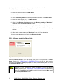
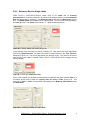
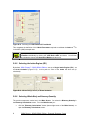
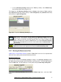
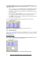
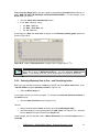
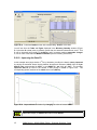
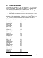
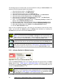
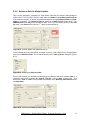
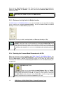
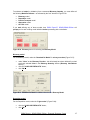
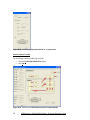
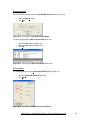
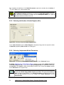
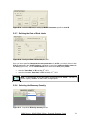
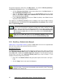
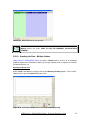
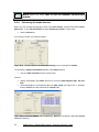
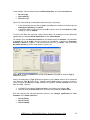
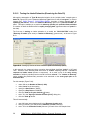
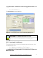
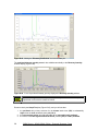
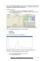
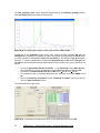
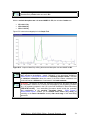
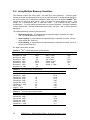
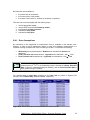
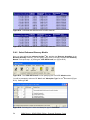
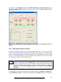
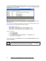
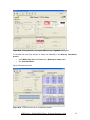
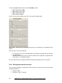
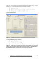
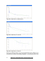
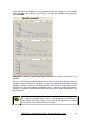
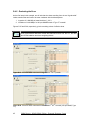
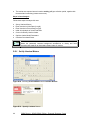
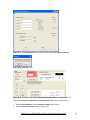
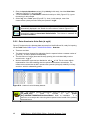
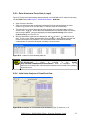
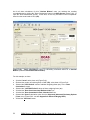
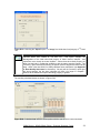
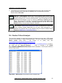

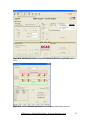
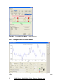
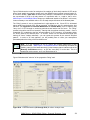
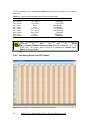
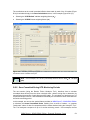
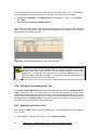
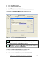

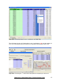
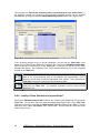
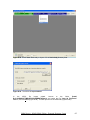
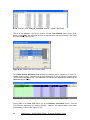
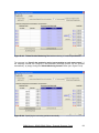
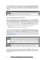
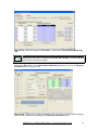
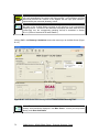
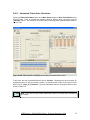
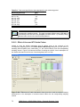
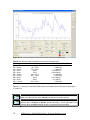
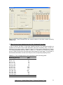
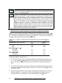
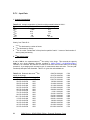
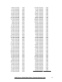
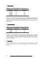
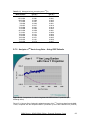
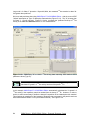
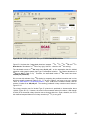
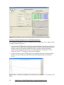
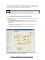
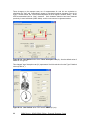
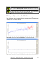
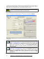
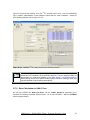
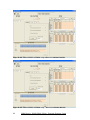
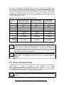
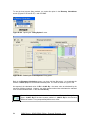
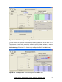
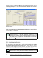
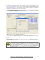
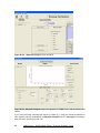
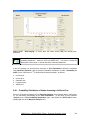
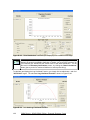
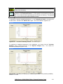
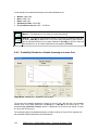
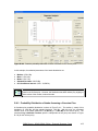
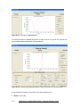
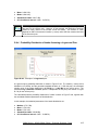
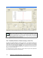
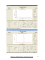
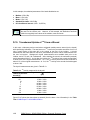
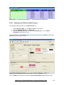
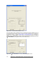
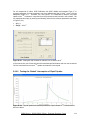
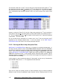
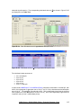
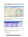
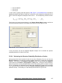
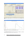
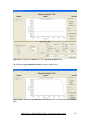
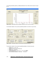
![User Manual [5.5 Mb - pdf]](http://vs1.manualzilla.com/store/data/005950654_1-5f0c3bfbdc0fa52796e7d9a416391587-150x150.png)