
1
HYDRUS
User Manual
Version 2
Software Package for Simulating
the Two- and Three-Dimensional Movement
of Water, Heat and Multiple Solutes
in Variably-Saturated Media
January 2011, PC-Progress, Prague, Czech Republic
© 2011 J.šimůnek and M. Šejna. All rights reserved
The HYDRUS Software Package for Simulating
the Two- and Three-Dimensional Movement
of Water, Heat, and Multiple Solutes
in Variably-Saturated Porous Media
User Manual
Version 2.04
M. Šejna1, J. Šimůnek2, and M. Th. van Genuchten3
July 2014
1
PC-Progress, Prague, Czech Republic
University of California Riverside, Riverside, CA
3
Department of Mechanical Engineering, Federal University of Rio de Janeiro, Brazil
2
© 2014 J. Šimůnek and M. Šejna. All rights reserved.
2
Table of Contents
Table of Contents................................................................................................................................. 3
List of Figures ...................................................................................................................................... 9
List of Tables ...................................................................................................................................... 17
Abstract .............................................................................................................................................. 19
Introduction to the HYDRUS Graphical User Interface .............................................................. 23
1. Project Manager and Data Management ................................................................................. 27
2. Projects Geometry Information ............................................................................................33
3. Flow Parameters ....................................................................................................................39
3.1.
Main Processes ............................................................................................................39
3.2.
Inverse Solution ...........................................................................................................42
3.3.
Time Information .........................................................................................................46
3.4.
Output Information ......................................................................................................48
3.5.
Iteration Criteria..........................................................................................................50
3.6.
Soil Hydraulic Model ...................................................................................................53
3.7.
Water Flow Parameters ...............................................................................................55
3.8.
Neural Network Predictions ........................................................................................59
3.9.
Anisotropy in the Hydraulic Conductivity ...................................................................60
3.10.
Solute Transport...........................................................................................................61
3.11.
Solute Transport Parameters .......................................................................................66
3.12.
Solute Reaction Parameters .........................................................................................67
3.13.
Temperature Dependence of Solute Transport Parameters ..........................................71
3.14.
Water Content Dependence of Solute Transport Parameters .......................................72
3.15.
Solution Compositions for the UNSATCHEM Module ..................................................73
3.16.
Chemical Parameters for the UNSATCHEM Module ...................................................74
3.17.
Heat Transport Parameters .........................................................................................75
3.18.
Root Water Uptake Model ...........................................................................................77
3.19.
Root Water Uptake Parameters ...................................................................................79
3.20.
Root Distribution Parameters ......................................................................................82
3.21.
Time Variable Boundary Conditions ...........................................................................84
3.22.
Constructed Wetlands ..................................................................................................87
3.23.
The Slope Stability Module ..........................................................................................97
3
4. Geometry of the Transport Domain ...................................................................................101
4.1.
Boundary Objects.......................................................................................................101
4.1.1. Points .............................................................................................................104
4.1.2. Lines and Polylines ........................................................................................107
4.1.3. Arcs and Circles .............................................................................................108
4.1.4. Curves and Splines .........................................................................................111
4.1.5. Common Information for a Graphical Input of Objects ................................113
4.1.6. Translate, Copy, Rotate, Mirror, Stretch, and Skew Operations...................114
4.1.7. Additional Operations....................................................................................117
4.2.
Surfaces .....................................................................................................................118
4.2.1. General Definitions. .......................................................................................118
4.2.1.1. Planar Surfaces ...............................................................................119
4.2.1.2. Curved Surfaces ..............................................................................121
4.2.1.3. Partial Surfaces ..............................................................................123
4.2.2. Steps to Define a Two-Dimensional Domain. ................................................123
4.2.3. Several notes on rules for correct definition of the Geometry. ......................124
4.2.4. Internal Objects. ............................................................................................125
4.2.5. Check and Repair Geometry. .........................................................................127
4.3.
Openings ....................................................................................................................121
4.4.
Solids .........................................................................................................................130
4.4.1. 3D-Layered – Hexahedral Solids...................................................................130
4.4.2. 3D-Layered – General Solids. .......................................................................131
4.4.2.1. Division of a Solid into Columns. ...................................................135
4.4.2.2. Division of a Solid into Geo-Layers................................................135
4.4.2.3. Individual specification of different Thicknesses of Geo-Layers at
different Thickness Vectors. ............................................................135
4.4.2.4. Steps to Define a 3D-Layered Domain. ..........................................136
4.4.3. 3D-General Solids. ........................................................................................136
4.5.
Thickness Vectors.......................................................................................................139
4.6.
Intersections of Surface and Solids ............................................................................143
4.7.
Auxiliary Objects .......................................................................................................143
4.7.1. Dimensions .....................................................................................................145
4
4.7.2. Labels .............................................................................................................146
4.7.3. Bitmaps (Textures) .........................................................................................147
4.7.4. Cross-Sections................................................................................................148
4.7.5. Mesh-Lines .....................................................................................................148
4.7.6. Background Layers ........................................................................................150
4.8.
Other Notes on Objects .............................................................................................153
4.8.1. Object Numbering ..........................................................................................153
4.8.2. Relations among Objects ...............................................................................153
4.8.3. References among Objects and Convention for Writing a List of Indices .....153
4.9.
Import Geometry from a Text File .............................................................................153
4.10.
Import Geometry from a DXF File ............................................................................156
4.11.
Import Geometry from a TIN File..............................................................................156
5. Finite Element Mesh ............................................................................................................157
5.1.
Finite Element Mesh Generator.................................................................................157
5.2.
Structured Finite Element Mesh Generator ...............................................................157
5.3.
Unstructured Finite Element Mesh Parameters ........................................................160
5.4.
Finite Element Mesh Refinement ...............................................................................168
5.4.1. Finite Element Mesh Refinement for MeshGen2D ........................................168
5.4.2. Finite Element Mesh Refinement for Genex/T3D ..........................................171
5.5.
Unstructured Finite Element Mesh Generator MeshGen2D .....................................174
5.6.
Finite Element Mesh Statistics ...................................................................................178
5.7.
Finite Element Mesh Sections......................................................................................... 179
6. Domain Properties, Initial and Boundary Conditions......................................................181
6.1.
Default Domain Properties ........................................................................................181
6.2.
Initial Conditions .......................................................................................................182
6.3.
Boundary Conditions .................................................................................................184
6.3.1. Time-Variable Head/Flux 1 BCs ...................................................................185
6.3.2. Special Boundary Conditions ........................................................................187
6.3.3. Triggered Irrigation .......................................................................................189
6.4.
Domain Properties .....................................................................................................191
6.5.
Defining Properties on Geometric Objects................................................................193
6.5.1. Materials on Geometric Objects ....................................................................195
6.5.2. Observation Nodes on Geometric Objects .....................................................198
5
6.5.3. Initial Conditions on Geometric Objects .......................................................199
6.5.4. Boundary Conditions on Geometric Objects .................................................200
6.5.5. Additional Notes on Properties at Geometric Objects ..................................201
6.6.
Import of Domain Properties and/or Initial and Boundary Conditions ....................202
6.6.1. Import Initial Condition from HYDRUS Projects..........................................202
6.6.2. Import Data from HYDRUS Projects ............................................................203
6.6.3. Import Data from a Text File .........................................................................204
7. Graphical Output .................................................................................................................209
7.1.
Results – Graphical Display ......................................................................................209
7.1.1. Displayed Variables .......................................................................................210
7.1.2. Display Options .............................................................................................215
7.1.3. Edit Isoband Value and Color Spectra ..........................................................216
7.1.4. Export Isolines ...............................................................................................222
7.2.
Results – Other Information.......................................................................................223
7.2.1. Convert to ASCII ............................................................................................226
8. Graphical User Interface Components ..............................................................................227
8.1.
View Window ............................................................................................................ 227
8.1.1
Scene and Viewing Commands ......................................................................227
8.1.2
Grid and Work Plane .....................................................................................228
8.1.3
Stretching Factors ..........................................................................................229
8.1.4. Rendering Model ...........................................................................................230
8.1.5. Selection and Edit Commands .......................................................................230
8.1.6. Pop-up Menus ..............................................................................................231
8.1.7. Drag and Drop ...............................................................................................232
8.1.8. Sections ..........................................................................................................232
8.2.
Navigator Bars ...........................................................................................................235
8.3.
Edit Bars ....................................................................................................................237
8.4.
Toolbars .....................................................................................................................242
8.5.
HYDRUS Menus.........................................................................................................246
8.6.
Input Tables in HYDRUS ...........................................................................................269
9. Miscellaneous Information..................................................................................................271
9.1.
Program Options .......................................................................................................271
9.2.
HYDRUS License and Activation...............................................................................275
6
9.2.1. Brief Description of HYDRUS Activation Using a Software Lock ................275
9.2.2. Detailed Description of HYDRUS Activation Using a Software Lock ..........275
9.2.2.1.
On-Line Activation ........................................................................278
9.2.2.2.
Activation by E-mail ......................................................................280
9.2.3. Reinstallation, Moving to another Computer ................................................286
9.2.3.1.
On-Line Deactivation ....................................................................287
9.2.3.2.
Deactivation by E-mail ..................................................................288
9.2.4. Extending Activation ......................................................................................289
9.2.5. Hardware Key ................................................................................................290
9.3.
Print Options..............................................................................................................292
9.4.
Print Preview and Copy to the Clipboard Commands ..............................................293
9.5.
Coordinate Systems ....................................................................................................294
9.6.
DOS Window During Calculations............................................................................295
9.7.
Running Computational Modules Outside of GUI or in a Batch...............................296
9.8.
The HyPar Module, a parallelized version ................................................................297
9.9.
Video Files .................................................................................................................298
9.10.
About HYDRUS..........................................................................................................300
References ...................................................................................................................................301
7
8
List of Figures
Figure 1. The HYDRUS Graphical User Interface (the main window). .....................................24
Figure 2. The project Manager with the Project Groups tab. ......................................................27
Figure 3. The Project Manager with the Projects tab. .................................................................28
Figure 4. The Project Information dialog window. .....................................................................30
Figure 5. General description of the HYDRUS Project Groups. .................................................30
Figure 6. The Domain Type and Units dialog window (with 3D preview). ................................33
Figure 7. Domain Type and Units dialog window (with 2D axisymmetrical preview). .............34
Figure 8. Examples of rectangular (top) and general (bottom) two-dimensional geometries. .....35
Figure 9. Example of a hexahedral three-dimensional geometry. ...............................................36
Figure 10. The Rectangular Domain Definition dialog window. ..................................................36
Figure 11. The Hexahedral Domain Definition dialog window. ..................................................37
Figure 12. The Main Processes dialog window. ..........................................................................40
Figure 13. The Inverse Solution dialog window. .........................................................................42
Figure 14. The Data for Inverse Solution dialog window. ...........................................................43
Figure 15. The Time Information dialog window. ............................................................................ 46
Figure 16. The Output Information dialog window. ......................................................................... 48
Figure 17. The Iteration Criteria dialog window. ..........................................................................50
Figure 18. The Soil Hydraulic Model dialog window...................................................................53
Figure 19. The Water Flow Parameters dialog window for direct (top) and inverse (bottom)
problems.......................................................................................................................55
Figure 20. The Rosetta Lite (Neural Network Predictions) dialog window. ................................59
Figure 21. The Edit Local Anisotropy dialog window for two-dimensional applications. ...........60
Figure 22. The Tensors of the Anisotropy dialog window............................................................60
Figure 23. The Solute Transport dialog window. ..........................................................................61
Figure 24. The Solute Transport dialog window for the UNSATCHEM module. .......................65
Figure 25. The Solute Transport Parameters dialog window. .......................................................66
Figure 26. The Solute Reaction Parameters dialog window. ........................................................67
Figure 27. The Solute Reaction Parameters dialog window for the UNSATCHEM module. ......70
Figure 28. The Temperature Dependent Solute Transport and Reaction Parameters dialog
window. ........................................................................................................................71
Figure 29. The Water Content Dependent Solute Reaction Parameters dialog window. .............72
9
Figure 30. The Solution Compositions dialog window for the UNSATCHEM module. .............73
Figure 31. The Chemical Parameters dialog window for the UNSATCHEM module. ................74
Figure 32. The Heat Transport Parameters dialog window...........................................................75
Figure 33. The Root Water Uptake Model dialog window. ..........................................................77
Figure 34. The Root Water Uptake Parameters dialog window for the stress response function of
Feddes et al. [1978] (left) and van Genuchten [1985] (right). .....................................79
Figure 35. The Root Water Uptake Parameters dialog window for the solute stress response
function based on the threshold model (left) and S-shape model of van Genuchten
[1985] (right)................................................................................................................80
Figure 36. The Root Distribution Parameters dialog window.......................................................83
Figure 37. The Time Variable Boundary Conditions dialog window. ..........................................84
Figure 38. The Constructed Wetland Model (CW2D) Parameter I dialog window......................89
Figure 39. The Constructed Wetland Model (CWM1) Parameter I dialog window. ....................92
Figure 40. The Constructed Wetland Model (CW2D) Parameter II dialog window. ...................93
Figure 41. The Constructed Wetland Model (CWM1) Parameter II dialog window....................95
Figure 42. The main window of the Slope Stability Module. .......................................................97
Figure 43. The Slope Stability Parameters dialog window. ..........................................................98
Figure 44. The Default Parameters for Slope Stability Module dialog window. ..........................99
Figure 45. An example of the Print and Export document generated by the Slope Stability
module........................................................................................................................100
Figure 46. A base surface showing several basic geometric objects...........................................104
Figure 47. The Edit Bar during the process of defining graphically a new point (left) and a new
line (right). .................................................................................................................105
Figure 48. The Edit Point dialog window. ..................................................................................106
Figure 49. Different ways of adding Parametric Points on a curve. ...........................................107
Figure 50. The Edit Curve dialog window. .................................................................................108
Figure 51. The Edit Bar during the process of defining graphically a radius for a new arc (left) or
a new circle (right). ....................................................................................................109
Figure 52. The New Line (Arc) dialog window. .........................................................................110
Figure 53. The New Line (Circle) dialog window. .....................................................................111
Figure 54. Edit Bar during the process of defining graphically a spline. ....................................112
Figure 55. Snap to a point (left) and snap to a curve (right). ......................................................113
Figure 56. The Translate - Copy dialog windows. ......................................................................114
Figure 57. The Rotate (left) and Mirror (right) dialog windows. ................................................115
10
Figure 58. The Stretch (left) and Skew (right) dialog windows. .................................................115
Figure 59. The Manipulation Options dialog window. The bitmaps indicate connecting lines between
points, surfaces between lines, and solids between surfaces. ............................................116
Figure 60. The Insert Point on Curve dialog window. ......................................................................117
Figure 61. The warning issued when Surfaces cannot be created automatically and must be
defined manually.................................................................................................................119
Figure 62. Edit Bar during the process of defining graphically a surface (left) and the General tab
of the Edit Surface dialog window (right). ................................................................119
Figure 63. A solid showing the base surface. ..............................................................................120
Figure 64. Solid showing separate vertical columns. ..................................................................120
Figure 65. A solid with its base surface in the XZ plane and thickness vectors in the Y direction.
....................................................................................................................................121
Figure 66. FE-Mesh for a solid with its base surface in the XZ plane and thickness vectors in the
Y direction..................................................................................................................121
Figure 67. Examples of Curved Surfaces (Rotary, Pipe, B-Spline, and Quadrangle Surfaces). .122
Figure 68. The Integrated Tab of the Edit Surface dialog window. ............................................125
Figure 69. An example of internal objects. .................................................................................126
Figure 70. An example of an Upper Surface definition using Internal Curves and Thickness
Vectors. ......................................................................................................................127
Figure 71. The Repair Domain Definition dialog window. ........................................................128
Figure 72. The New Opening dialog window. ............................................................................129
Figure 73. The Edit Bar during the process of graphically defining a Hexahedral Solid.
Definition of a Base Surface on the left and a Thickness on the right.......................130
Figure 74. The Edit Bar during the process of graphically defining a Solid by extruding a Base
Surface. Selection of a Surface (left) and definition of a Thickness Vector (right). .131
Figure 75. The 3D-Layered Solid dialog window; the General, Geo-Layers, and Thickness
Profiles Tabs. .............................................................................................................133
Figure 76. The 3D-Layered Solid dialog window; the FE-Mesh Tab for single and multiple
layers. .........................................................................................................................134
Figure 77. Examples of 3D-General Solids. Top - formed by Planar Surfaces, bottom – formed
by curved surfaces......................................................................................................137
Figure 78. Edit Bar during the process of graphically defining a Thickness Vector. .................140
Figure 79. The Thickness dialog window. ..................................................................................140
Figure 80. A solid with several thickness vectors. ......................................................................141
Figure 81. FE-Mesh for the solid in Figure 80. ...........................................................................141
Figure 82. Missing internal curves in the base surface. ..............................................................142
11
Figure 83. Consequence of missing an internal curve in the base surface on the FE-Mesh of the
top surface. .................................................................................................................142
Figure 84. The Edit Intersection dialog window (for two Surfaces (left) and two Solids (right).143
Figure 85. An example of an Intersection of two Surfaces and a resulting Partial Surface and
Intersection Curve. .....................................................................................................144
Figure 86. Edit Bar during the process of graphically defining a Dimension. Selection of two
definition points, the distance of which is to be labeled (left) and the dimension type
(right). ........................................................................................................................145
Figure 87. The Edit Comment dialog window. ...........................................................................146
Figure 88. The Edit Bar during the process of graphically defining a Comment. Selection of the
Comment Position, Comment Text, Font and Color (left) and Offset (right). ..........147
Figure 89. The Edit Bitmap dialog window. ...............................................................................147
Figure 90. The Cross-Section dialog window. ............................................................................148
Figure 91. The Mesh-Line dialog window. .................................................................................149
Figure 92. The Fluxes across Mesh-Line dialog window. ..........................................................149
Figure 93. An example of the Background Layer. ......................................................................151
Figure 94. The New Background Layer dialog window. ............................................................151
Figure 95. The Import Geometry from a DXF File dialog window. ...........................................156
Figure 96. The Rectangular Domain Discretization dialog window. ..........................................158
Figure 97. The Hexahedral Domain Discretization dialog window. ...........................................159
Figure 98. The FE-Mesh Parameters dialog window (the Main Tab for 3D-Layered (left) and
3D-General (right) geometries)..................................................................................160
Figure 99. The FE-Mesh Parameters dialog window (Tab Stretching). .....................................161
Figure 100. The Mesh Stretching dialog window for a Local FE-Mesh Stretching. .................162
Figure 101. Listing of FE-Mesh Stretchings on the Navigator Bar. ..........................................162
Figure 102. An example of the FE-Mesh with three FE-Mesh Stretchings assigned to areas
below the domain surface. ......................................................................................163
Figure 103. The FE-Mesh Parameters dialog window (Tab MG Options). ...............................164
Figure 104. The FE-Mesh Parameters dialog window (Tab Options). ......................................166
Figure 105. The FE-Mesh Parameters dialog window (Mesh Section Tab). .............................167
Figure 106. The New FE-Mesh Refinement dialog window for the MeshGen2D module with
four different types of refinements (applied to a Point, a Line with a given FE-size
or the number of Points, and to a Surface)..............................................................169
Figure 107. Example of FE-Mesh Refinements (top) and FE-Mesh (bottom). .........................170
Figure 108. Circular (left) and rectangular (right) refinements around a node. .........................171
12
Figure 109. Refinement on a line (by defining either the size or the number of finite elements
along a line).............................................................................................................172
Figure 110. Refinements on a surface (left) or solid (right). ......................................................172
Figure 111. The FE-Mesh Refinement dialog window for the Genex/T3D module with six
different types of refinements (applied to a Circular or a Rectangular Point, a Line
with a given FE-size or a number of points, to a Surface, and to a Solid)..............174
Figure 112. Example of mesh stretching using a stretching factor of 3 in the x-direction. ..........177
Figure 113. The FE-Mesh Information dialog window for a two-dimensional problem (top) and
a three-dimensional problem (bottom)....................................................................178
Figure 114. The FE-Mesh Sections dialog window. ..................................................................180
Figure 115. The Default Domain Properties dialog window. ....................................................182
Figure 116. The Water Flow Initial Condition dialog window. .................................................183
Figure 117. The Temperature distribution dialog window.........................................................184
Figure 118. The Time-Variable Head/Flux 1 BCs tab of the Boundary Condition Options dialog
window. ...................................................................................................................186
Figure 119. The Special Boundary Conditions tab of the Boundary Condition Options dialog
window. ...................................................................................................................189
Figure 120. The Triggered Irrigation tab of the Boundary Condition Options dialog window. 190
Figure 121. The Stochastic Distribution of Scaling Factors dialog window. .............................191
Figure 122. The Stochastic Parameters dialog window. ............................................................192
Figure 123. An example of the transport domain defined using three components S1, S2, and
S3. ...........................................................................................................................193
Figure 124. The upper part of the Edit Bar, which displays defined materials and commands for
various actions with materials. ................................................................................195
Figure 125. The Set Materials dialog window. ..........................................................................196
Figure 126. The transport domain with materials specified on geometric objects. ....................196
Figure 127. The Sort Property Objects dialog window. .............................................................197
Figure 128. The Edit Materials dialog window. .........................................................................198
Figure 129. The Observation Node dialog window. ..................................................................199
Figure 130. The Edit Pressure Head (left) and Concentration (right) Initial Conditions dialog
window. ...................................................................................................................200
Figure 131. The Edit Water Flow Boundary Condition dialog window. ...................................201
Figure 132. The Import Initial Condition dialog window. .........................................................202
Figure 133. The Import Selected Quantities dialog window......................................................203
Figure 134. The Import of Values from Scattered Points dialog window. ................................206
13
Figure 135. The "Results - Graphical Display" part of Data Tab of the Navigator Bar for the
standard (left), Unsatchem (centre), and Wetland (right) modules.........................213
Figure 136. The "Results" part of the View Tab of the Navigator Bar with the display of various
alternative variables. ...............................................................................................214
Figure 137. The Display Options dialog window. .....................................................................215
Figure 138. The Edit Isoband Value and Color Spectra dialog window. ...................................216
Figure 139. The use of intermediate isolines. ............................................................................217
Figure 140. The Color dialog window. ......................................................................................218
Figure 141. Adjusting scale in the Edit Isoband Value and Color Spectra dialog window. ......219
Figure 142. The use of the Custom Scale. ..................................................................................220
Figure 143. The color smoothing. ..............................................................................................221
Figure 144. An
example of
the Project_Property_Isolines.txt
text
file (e.g.,
Furrow_Pressure_Head_Isolines.txt; an excerpt) for the Furrow project (displayed
in the top of the figure). ..........................................................................................222
Figure 145. x-y graph dialog window displaying pressure heads in observation nodes. ...........223
Figure 146. The Convert to ASCII dialog window. ...................................................................226
Figure 147. The Grid and Work Plane dialog window. .............................................................228
Figure 148. The View Stretching Factors dialog window. .........................................................229
Figure 149. The Rendering part of the View Tab of the Navigator Bar. ...................................230
Figure 150. The Pop-up Menu from the View window. ............................................................232
Figure 151. Options for Generation of Geo-Sections and FE-Mesh Sections dialog window. .233
Figure 152. Selected Navigator Bars (Data Tabs on the left and in the middle, the View Tab
on the right). ............................................................................................................236
Figure 153. Selected Edit Bars (from left to right) for Material Distribution in Domain
Properties, Water Flow Boundary Conditions, Pressure Head Initial Conditions, and
Water Content Results. ...........................................................................................237
Figure 154. The Color Scale Display Options menu..................................................................241
Figure 155. Selected Edit Bars (for Domain Geometry and FE-Mesh). ....................................241
Figure 156. The Toolbars dialog window. .................................................................................242
Figure 157. The Customize Toolbars dialog window. ...............................................................242
Figure 158. The HYDRUS Menus I (File, Edit, and View). ......................................................246
Figure 159. The HYDRUS Menus II (Insert, Calculations, and Results). .................................247
Figure 160. The HYDRUS Menus II (Tools, Options, Windows, and Help). ...........................247
Figure 161. The Program Options dialog window (the Graphics Tab). .....................................271
Figure 162. The Program Options dialog window (the Program Tab).......................................272
14
Figure 163. The Program Options dialog window (the FE-Mesh Tab). ....................................273
Figure 164. The Program Options dialog window (the Files and Directories Tab). ..................274
Figure 165. The HYDRUS Authorization Status dialog window (Tab Status). ........................276
Figure 166. Warning issued when attempting to make changes to the Authorization Status while
not running HYDRUS with administrator privileges.. ...........................................277
Figure 167. The HYDRUS Authorization Status dialog window (Tab Add-on Modules). .......277
Figure 168. The HYDRUS License and Activation dialog window (Tab History of Activation).
.................................................................................................................................278
Figure 169. The Online Activation dialog window. ...................................................................279
Figure 170. Window requesting confirmation of entered parameters. .......................................280
Figure 171. The Activation by E-mail dialog window (Tab Step 1).. ........................................293
Figure 172. The Activation by E-mail dialog window (Tab Step 2). .........................................282
Figure 173. Email with the HYDRUS Activation Request in Outlook......................................283
Figure 174. Window inquiring if the user wants to enter the Activation Code..........................284
Figure 175. The Activation by E-mail dialog window (Tab Step 3). .........................................285
Figure 176. Window confirming successful HYDRUS authorization. ......................................285
Figure 177. Window reporting a failure of HYDRUS authorization. ........................................286
Figure 178. The Online Deactivation dialog window. ...............................................................287
Figure 179. Window confirming successful online deactivation of HYDRUS. ........................287
Figure 180. The HYDRUS Deactivation dialog window. ..........................................................288
Figure 181. Window confirming successful deactivation of HYDRUS by email. ....................289
Figure 182. The HYDRUS 2.xx Setup window with a choice to install the hardware-key driver .
.................................................................................................................................290
Figure 183. The General, Picture, and Legend tabs of the Print Options dialog window..........292
Figure 184. The Coordinate Systems dialog windows. ..............................................................294
Figure 185. The Create Video File dialog window. ...................................................................298
Figure 186. Result of commands Print Preview or Copy to the Clipboard. ...............................293
Figure 187. The About HYDRUS dialog window (the Program tab (top) and the Authors tab
(bottom)...................................................................................................................300
15
16
List of Tables
Table 1.
Commands in the Project Manager. .............................................................................29
Table 2.
Data types for the objective function (Inverse Problem). ............................................44
Table 3.
Definition of the column X in Fig. 14 based on Data Type (Inverse Problem). ............44
Table 4.
Definition of the column Y in Fig. 14 based on Data Type (Inverse Problem)..............45
Table 5.
Time Information variables. .........................................................................................47
Table 6.
Time Step Control variables. ........................................................................................52
Table 7.
Soil hydraulic parameters for the analytical functions of van Genuchten [1980] for
twelve textural classes of the USDA soil textural triangle according to Carsel and
Parrish [1988]..............................................................................................................57
Table 8.
Soil hydraulic parameters for the analytical functions of van Genuchten [1980] for
twelve textural classes of the USDA textural triangle as obtained with the Rosetta
Lite program [Schaap et al., 2001]. .............................................................................57
Table 9.
Soil hydraulic parameters for the analytical functions of Brooks and Corey [1964] for
twelve textural classes of the USDA soil textural triangle according to Carsel and
Parrish [1988]..............................................................................................................58
Table 10. Soil hydraulic parameters for the analytical functions of Kosugi [1996] for twelve
textural classes of the USDA soil textural triangle. .....................................................58
Table 11. Comparison of CW2D and CWM1 components. ........................................................87
Table 12. Comparison of CW2D and CWM1 processes. ............................................................88
Table 13. Kinetic parameters in the CW2D biokinetic model [Langergraber and Šimunek,
2005]. ...........................................................................................................................90
Table 14. Kinetic parameters in the CWM1 biokinetic model [Langergraber et al., 2009]. ......91
Table 15. Temperature dependences, stoichiometric parameters, composition parameters and
parameters describing oxygen transfer in the CW2D biokinetic model [Langergraber
and Šimunek, 2005]......................................................................................................94
Table 16. Temperature dependences, stoichiometric parameters, composition parameters and
parameters describing oxygen transfer in the CWM1 biokinetic model [Langergraber
et al., 2009]. .................................................................................................................96
Table 17. Definition of terms related to geometry design. ..........................................................102
Table 18. Definition of terms related to boundary discretization. ...............................................175
Table 19. Finite element mesh sections generated in different HYDRUS versions. ...................179
Table 20. Definition of commands used to manipulate Property Objects. ................................194
Table 21. Standard variables displayed in the View Window of the Results tab (Results Graphical Display). ....................................................................................................210
Table 22. Alternative variables that can be displayed in the View Window of the Results tab.211
17
Table 23. Definition of various concentration modes (for linear sorption model). ...................212
Table 24. Graph options in the HYDRUS interface. .................................................................224
Table 25. HYDRUS menu commands. ......................................................................................248
Table 26. Brief description of HYDRUS menu commands.......................................................256
Table 27. A comparison of the HyPar module to standard computational modules. ...................297
18
Abstract
Šejna, M., J. Šimůnek, and M. Th. van Genuchten, The HYDRUS Software Package for Simulating
Two- and Three-Dimensional Movement of Water, Heat, and Multiple Solutes in VariablySaturated Porous Media, User Manual, Version 2.04, PC Progress, Prague, Czech Republic, 305 pp.,
2014.
This report documents version 2.0 of the Graphical User Interface of HYDRUS, a software
package for simulating water, heat, and solute movement in two- and three- dimensional variably
saturated porous media. The software package consists of the computational computer program, and
the interactive graphics-based user interface. The HYDRUS program numerically solves the
Richards equation for variably saturated water flow and advection-dispersion equations for both
heat and solute transport. The flow equation incorporates a sink term to account for water uptake by
plant roots. The heat transport equation considers transport due to conduction and convection with
flowing water. The solute transport equations consider advective-dispersive transport in the liquid
phase, as well as diffusion in the gaseous phase. The transport equations also include provisions for
nonlinear nonequilibrium reactions between the solid and liquid phases, linear equilibrium reactions
between the liquid and gaseous phases, zero-order production, and two first-order degradation
reactions. In addition, physical nonequilibrium solute transport can be accounted for by assuming a
two-region, dual-porosity type formulation which partitions the liquid phase into mobile and
immobile regions. Attachment/detachment theory, including filtration theory, is additionally
included to enable simulations of the transport of viruses, colloids, and/or bacteria.
HYDRUS may be used to analyze water and solute movement in unsaturated, partially saturated, or
fully saturated porous media. The program can handle flow regions delineated by irregular
boundaries. The flow region itself may be composed of nonuniform soils having an arbitrary degree
of local anisotropy. Flow and transport can occur in the two-dimensional vertical or horizontal plane,
a three-dimensional region exhibiting radial symmetry about the vertical axis, or a fully threedimensional domain. The two-dimensional part of this program also includes a MarquardtLevenberg type parameter optimization algorithm for inverse estimation of soil hydraulic and/or
solute transport and reaction parameters from measured transient or steady-state data for two
dimensional problems. Details of the various processes and features included in HYDRUS are
provided in the Technical Manual [Šimůnek et al., 2011].
The main program unit of the HYDRUS Graphical User Interface (GUI) defines the overall
computational environment of the system. This main module controls execution of the program and
determines which other optional modules are necessary for a particular application. The module
contains a project manager and both the pre-processing and post-processing units. The preprocessing unit includes specification of all necessary parameters to successfully run the HYDRUS
FORTRAN codes, grid generators for relatively simple rectangular and hexahedral transport
domains, a grid generator for unstructured finite element meshes for complex two-dimensional
domains, a small catalog of soil hydraulic properties, and a Rosetta Lite program for generating soil
hydraulic properties from soil textural data. The post-processing unit consists of simple x-y graphics
for graphical presentation of soil hydraulic properties, as well as such output as distributions versus
19
time of a particular variable at selected observation points, and actual or cumulative water and
solute fluxes across boundaries of a particular type. The post-processing unit also includes options
to present results of a particular simulation by means of contour maps, isolines, spectral maps, and
velocity vectors, and/or by animation using both contour and spectral maps.
Version 2.0, which includes the 3D-Professional Level of HYDRUS, includes many new features as
compared to version 1.0. New features and changes in the HYDRUS GUI:
1) Supports for complex general three-dimensional geometries (Professional Level).
2) Domain Properties, Initial Conditions, and Boundary Conditions can be specified on
Geometric Objects (defining the transport domain) rather than on the finite element mesh.
3) Import of initial conditions from existing HYDRUS projects even with (slightly) different
geometry or FE mesh.
4) Import of various quantities (e.g., domain properties, initial and boundary conditions)
from another HYDRUS projects even with (slightly) different geometry or FE mesh.
5) Support of ParSWMS (a parallelized version of SWMS_3D).
6) Support of UNSATCHEM (a module simulating transport of and reactions between
major ions).
7) The Mass Balance (Inverse) Information dialog window enables to display texts larger
than the capacity of the Edit window.
8) Root distribution can be specified using GUI parallel with the slope for hillslopes.
9) Display of results using Isosurfaces.
10) Support of a new CWM1 constructed wetland module [Langergraber et al., 2009].
New features and changes in the HYDRUS in the computational modules:
1) New initializations conditions for solute transport (initial conditions can be specified in the
total solute mass and nonequilibrium phases can be initially equilibrated).
2) Various new boundary conditions (e.g., gradient, surface drip, subsurface drip, and seepage
face with a specified pressure head boundary conditions).
3) Triggered Irrigation - irrigation is triggered by the program when the pressure head at a
particular observation node drops below a specified value.
4) HYDRUS calculates and reports surface runoff, evaporation and infiltration fluxes for the
atmospheric boundary.
5) Water content dependence of solute reactions parameters using the Walker’s [1974] formula
was implemented.
6) A new option to consider root solute uptake, including both passive and active uptake
[Šimůnek and Hopmans, 2009].
7) The Per Moldrup’s tortuosity models [Moldrup et al., 1997, 2000] were implemented as
an alternative to the Millington and Quirk [1961] model.
8) An option to use a set of Boundary Condition records multiple times.
9) Executable programs are about 1.5 - 3 times faster than in the standard version due to the
loop vectorization.
10) Options related to the fumigant transport (e.g., removal of tarp, temperature dependent
tarp properties, additional injection of fumigant).
11) A new CWM1 constructed wetland module [Langergraber et al., 2009].
Version 2.02 additionally supports several add-on modules that have their own user manuals, such
20
as the DualPerm module [Šimůnek et al., 2012e], the UNSATCHEM module [Šimůnek et al.,
2012c], the Wetland module [Langergraber and Šimůnek, 2011], the C-Ride module [Šimůnek et
al., 2012b], and the HP2 module [Šimůnek et al., 2012a].
Version 2.03 offers some new functionality with respect to the import of various properties from
either existing HYDRUS projects or from text files (see Section 6.6), allows users to import
definition of isolines (only in 3D-Professional) and resolves problems with fonts for the Chinese,
Japanese, and other similar Windows systems.
Version 2.04 additionally supports two add-on modules, such as the HyPar module (see Section
9.1) and the Slope Stability module. While the HyPar module is a parallelized version of the
standard two-dimensional and three-dimensional HYDRUS computational modules
(h2d_calc.exe and h3d_calc.exe), the Slope Stability module is intended to be used mainly for
stability checks of embankments, dams, earth cuts and anchored sheeting structures.
This report serves as a User Manual and reference document of the Graphical User Interface of
the HYDRUS software package. Technical aspects such as governing equations and details about
the invoked numerical techniques are documented in a separate Technical Manual.
21
22
Introduction to the HYDRUS Graphical User Interface
The past several decades or so has seen an explosion of increasingly sophisticated numerical models
for simulating water flow and contaminant transport in the subsurface, including models dealing
with one- and multi-dimensional flow and transport processes in the unsaturated or vadose zone
between the soil surface and the ground water table. Even with an abundance of well-documented
models now available, one major problem often preventing their optimal use is the extensive work
required for data preparation, numerical grid design, and graphical presentation of the output results.
Hence, the more widespread use of multi-dimensional models requires ways which make it easier to
create, manipulate and display large data files, and which facilitate interactive data management.
Introducing such techniques will free users from cumbersome manual data processing, and should
enhance the efficiency in which programs are being implemented for a particular example. To avoid
or simplify the preparation and management of relatively complex input data files for two- and
three-dimensional applications, and to graphically display the final simulation results, we developed
an interactive graphics-based user-friendly interface HYDRUS for the MS Windows 95, 98, NT,
ME, XP, Vista, and 7 environments. The interface is connected directly to the computational codes.
The current version 2.0 of the HYDRUS graphical user interface represents a major upgrade of
version 1.0, which itself was a complete rewrite of the version 2.0 of HYDRUS-2D that expanded
capabilities of HYDRUS-2D to three-dimensional problems. Version 2, which includes the 3DProfessional Level of HYDRUS, includes many new features as compared to version 1.0. In
particular, it includes support for complex general three-dimensional geometries and an option to
specify various domain properties, and initial and boundary conditions on geometric objects, rather
than directly on the finite element mesh.
In addition to information given in this user manual, extensive context-sensitive on-line help is
made part of the graphical user interface (GUI). By holding the F1 button or clicking on the Help
button while working in any window, the user obtains information about the window content. In
addition, context-sensitive help is available in every module using the "SHIFT+F1" help button. In
this mode, the mouse cursor changes to a help cursor (a combination arrow + question mark), which
a user can use to select a particular object for which help is needed (e.g., a menu item, toolbar button,
or other features). At that point, a help file will be displayed giving information about the item on
which the user clicked. Except for the computational modules that are written in FORTRAN, the
entire GUI is written in C++.
The HYDRUS Graphical User Interface (Fig. 1) is the main program unit defining the overall
computational environment of the system. This main module controls execution of the program and
determines which other optional modules are necessary for a particular application. The module
contains a project manager and both the pre-processing and post-processing units. The preprocessing unit includes specification of all necessary parameters to successfully run the HYDRUS
FORTRAN codes (modules H2D_CALC, H2D_CLCI, H2D_WETL, H2D_UNSC, and/or
H3D_CALC), grid generators for relatively simple rectangular and hexahedral transport domains, a
grid generator for unstructured finite element meshes appropriate for more complex twodimensional domains, a small catalog of soil hydraulic properties, and a Rosetta Lite program for
generating soil hydraulic properties from textural information. The post-processing unit consists of
simple x-y graphs for graphical presentation of the soil hydraulic properties, distributions versus
time of a particular variable at selected observation points, as well as actual or cumulative water and
23
solute fluxes across boundaries of a particular type. The post-processing unit also includes options
to present results of a simulation by means of contour maps, isolines, isosurfaces, spectral maps, and
velocity vectors, and/or by animation using both contour and spectral maps.
Figure 1. The HYDRUS Graphical User Interface (the main window).
Figure 1 shows the main window of the HYDRUS graphical user interface, including its main
components such as the Menu, Toolbars, the View Window, the Navigator Bar, Tabs, and the
Edit Bar. These terms will be used throughout this user manual. The text below provides a
detailed description of all major components of the graphical user interface. At the end of this
user manual a list is given of all commands accessible through the menu (Table 25), as well as a
brief discussion of the action taken with particular commands (Table 26). More detailed
descriptions are available through the on-line help.
Work for a new project should begin by opening the Project Manager (see Chapter 1), and giving a
name and brief description to the new project. Next the Domain Type and Units dialog Window
(Figs. 6 and 7) appears (this window can be also selected from the Pre-processing Menu). From this
point on the program will navigate users through the entire process of entering input files. Users
may either select particular commands from a menu, or allow the interface to lead them through the
process of entering input data by selecting the Next button. Alternatively, clicking the Previous
button will return users to the previous window. Pre- and post processing commands and processes
24
are also sequentially listed on the Data Tab of the Navigator Bar. Green arrows on the Edit Bar
always direct users to subsequent or previous input processes for a particular command. Many
commands and processes can be alternatively accessed using either the Toolbars and Menus, or the
Navigator and Edit Bars.
25
26
1. Project Manager and Data Management
A Project Manager (called by the command File->Project Manager, Figs. 2 and 3) is used to
manage the data of existing projects, and helps to locate, open, copy, delete and/or rename desired
projects or their input or output data. A Project represents any particular problem to be solved by
HYDRUS. The project name, as well as a brief description of the project (Fig. 4), helps to locate a
particular problem. Projects are represented by a file project_name.h3d2 (the final 2 refers to
version 2 of HYDRUS; extension h3d was used with version 1.0) that contains all input and output
data when the Temporary Working Directory option (Fig. 4) is used. It contains only the input data
when the Permanent Working Directory option is selected. HYDRUS input files (used by the
computational modules) are extracted from the project_name.h3d2 file into a working subdirectory;
output data created by the calculation module are sent into the same folder. When saving a project,
output files (created by the computational modules) are also included into the project_name.h3d2
file (when the Temporary Working Directory option is used). The input and output files can be
either permanently kept in the external working directory, or are stored in this folder only during
calculations (Fig. 4, the radio buttons Temporary – is deleted after closing the project and
Permanent – result files are kept in this directory). The location of the external working directory is
specified in the Project Description (Fig. 4) and the Program Options dialog window (Fig.
162).
Figure 2. The project Manager with the Project Groups tab.
27
Figure 3. The Project Manager with the Projects tab.
The Project Manager gives users considerable freedom in organizing their projects. The projects
are grouped into Project Groups (Fig. 2), which can be placed anywhere in accessible memory (i.e.,
on local and/or network hard drives). Project Groups serve to organize projects into logical groups
defined by a user. Each Project Group has its own name, description, and pathway (Figs. 2 and 5).
A Project Group can be any existing accessible subdirectory (folder). HYDRUS is installed
together with two default Project Groups, 2D_Tests and 3D_Tests, which are located in the
HYDRUS3D folder. The 2D_Tests and 3D_Tests Project Groups contain test examples for two- and
three-dimensional problems, respectively. We suggest that users create their own Project Groups
(e.g., the My_2D_Direct, My_2D_Inverse, and My_3D_Direct Project Groups), and keep the
provided examples intact for future reference. Projects can be copied with the Project Manager
only within a particular Project Group. Users can copy projects between Project Groups (or share
28
their HYDRUS projects with colleagues and clients) using standard file managing software, such as
Windows Explorer. In that case one must copy only the project_name.h3d2 file (when the radio
buttons Temporary – is deleted after closing the project is used, Fig. 4). When temporary data are
kept permanently in the working directory (i.e., the radio button Permanent – results files are kept
in this directory is selected, Fig. 4), the working directory must be copied together with the
project_name.h3d2 file.
In addition to a Name and a brief Description of a Project, the Project Manager also displays
dimensions for a particular problem (Type: the dimensions are either 2D or 3D, and the geometry is
either Simple (S), Layered (L), or General (G), see Section 2), what Processes are involved (W –
water flow, S – solute transport, T – heat transport, R – root water uptake, Inv – Inverse problem),
the size of the project (MB), when the project was created (Date) and whether or not the Results
exist (Fig. 3). The Project Manager can also display a preview of the Project’s geometry (see
the check box Show Project Preview in Fig. 3). Commands of the Project Manager are listed in
Table 1.
Table 1. Commands in the Project Manager.
Group
Command
Description
Project Group New
Edit
Registers a new Project Group in the Project Manager.
Renames the selected Project Group, and changes its description
and/or location.
Remove
Removes registration of a selected Project Group from the Project
Manager.
Set As Current Sets a selected Project Group as the active Project Group.
Close
Closes the Project Manager.
Project
New
Copy
Rename
Delete
Open
Close
Convert
Calculate
Creates a new project in the current Project Group.
Copies a selected project within the current Project Group.
Renames a selected project.
Deletes a selected project.
Opens a selected project.
Closes the Project Manager.
Converts projects created by earlier HYDRUS versions (i.e., either
HYDRUS-2D or version 1.0 of HYDRUS (2D/3D)).
Calculates selected HYDRUS projects. This command allows
users to calculate multiple selected projects simultaneously.
Options
Description
Show Project Preview
Provides a preview of the geometry of a particular project in the
bottom left corner of the Project Manager.
Shows projects created using earlier HYDRUS versions, i.e.,
either HYDRUS-2D or version 1.0 of HYDRUS (2D/3D).
Opens the Project Manager at the Project Groups Tab.
Show Old Projects
Start on Project Groups Page
29
The commands New and Rename from the Project Tab of the Project Manager dialog window
(Fig. 3) call the Project Information dialog window (Fig. 4), which contains the Name and
Description of the project, as well as information about the Project Group (name, description, and
pathway) to which the project belongs. It also contains information whether or not the input and
output data are kept permanently in an external directory (the radio buttons Temporary – is
deleted after closing the project and Permanent – result files are kept in this directory, Fig. 4).
Figure 4. The Project Information dialog window.
Figure 5. General description of the HYDRUS Project Group.
Projects created by the previous versions of HYDRUS (e.g., HYDRUS-2D) can be imported into
the current version of HYDRUS using two ways:
30
A. Individual projects can be converted using the command File->Import and Export->Import
HYDRUS-2D Project. This is done by first creating a new Project, and then selecting the
above command and browsing for the location of a project created with a previous version of
HYDRUS-2D. The input data of the older project are then converted into the new HYDRUS
format. Results of the older project can then be viewed using the new version of HYDRUS,
while projects can be modified or recalculated as needed.
B. Multiple HYDRUS-2D projects (or HYDRUS projects created by earlier versions of
HYDRUS) can be converted simultaneously using the Convert command of the Project
Manager. One first creates a HYDRUS Project Group for a folder in which the HYDRUS-2D
projects are located and selects the Show Old Projects option at the Project Tab of the
Project Manager. One then selects projects to be converted and clicks the Convert command.
HYDRUS in this way creates HYDRUS projects and stores all input and output files in the
project_name.h3d2 files.
Input data can be edited either using the HYDRUS graphical user interface (this modifies directly
the project_name.h3d2 file) or the input data can be modified manually. In such case, HYDRUS
input files need to be stored in the working external directory (sent there by the command File>Import and Export->Export Data for HYDRUS Solver), and then can be imported back into the
HYDRUS project_name.h3d2 file using the command File->Import and Export->Import Input
Data from *.In Files.
The Working Directory is a folder into which the program stores temporary data. Each open
project has its own Working Directory, where the program stores, for example, input files for
computational modules, and where computational modules write the output files. When saving a
project, data from the Working Directory are copied into the main project file project_name.h3d2.
When the project is closed, the Working Directory is deleted. Only when a user selects the option
“Permanent – result files are kept in this directory” (Fig. 4) is the Working Directory not deleted
after closing the project, in which case the temporary data are not copied into the main project file.
31
32
2. Projects Geometry Information
In the first dialog window that a user encounters after creating a new project, he/she needs to
specify whether the flow and transport problem occurs in two- or three-dimensional transport
domains. Geometry type is selected in the Domain Type and Units dialog Window (Fig. 6 and
7). In this dialog window, users specify the Type of Geometry, the 2D Domain Options, the
Length Units, and the size of the Initial Project Group (the approximate size of the transport
domain).
Type of Geometry: This section allows a user to choose between simple geometries having a
structured finite element mesh (i.e., 2D-Simple (Parametric) and 3D-Simple (Parametric)), or
more general geometries having an unstructured finite element mesh (i.e., 2D-General (Boundary
Rep.), 3D-Layered, and 3D-General (Boundary Rep.)). Available options depend on the level of
authorization (purchased License). Only simple geometries 2D-Simple (Parametric) and 3DSimple (Parametric) are available for HYDRUS Levels 2D-Lite and 3D-Lite, respectively. 2DGeneral (Boundary Rep.) is available for the 2D-Standard Level, 3D-Layered for the 3DStandard Level, and 3D-General (Boundary Rep.) for the 3D-Professional Level.
Figure 6. The Domain Type and Units dialog window (with 3D preview).
33
Figure 7. The Domain Type and Units dialog window (with 2D axisymmetrical preview).
There are two types of two-dimensional transport domains (Surfaces, see also Section 4.2)
depending upon the selection made in the Domain Type and Units dialog window (Fig. 6 and 7):
•
2D-Simple (Parametric): This type of solid has a Rectangular Shape and is defined by
its basic dimensions. Rectangular domains are defined by three straight lines, one at the
bottom of the domain and two at the sides, whereas the upper boundary may or may not be
straight. Nodes along the upper boundary line may in that case have variable x- and zcoordinates. However, the lower boundary line must always be horizontal (or have a
specified slope), while the left and right boundary lines must be vertical. The flow region is
then discretized into a structured triangular mesh. Examples of simple rectangular
geometries are shown in Figure 8 (top).
•
2D-General (Boundary Rep.): This type of Surface is defined by a set of Boundary
Curves see Section 4.2). Examples of general two-dimensional geometries are shown in
Figure 8 (bottom) and Figure 46.
There are three types of three-dimensional transport domains (Solids, see also Section 4.4)
depending upon the selection made in the Domain Type and Units dialog window (Fig. 6 and 7):
34
•
3D-Simple (Parametric): This type of solid has a Hexahedral Shape and is defined by
its basic dimensions. The base can have a certain slope in the X and Y dimensions (Fig.
9). Hexahedral domains must have similar properties as rectangular domains, i.e., vertical
planes at the sides, a horizontal (or with a specified slope) plane at the bottom boundary, and
with only the upper boundary not needing to be a plane. An example of a simple hexahedral
three-dimensional geometry (i.e., 3D-Simple) is given in Figure 9.
•
3D-Layered: This type of solid is defined by the Base Surface (see Section 4.2) and one
or more Thickness Vectors (see Section 4.5).
•
3D-General (Boundary Rep.): This type of solid is defined using a set of surfaces that
fully form its boundaries. This type of geometries is available only in the 3DProfessional version. 3D-General Geometries can be formed from three-dimensional
objects (Solids) of general shapes. Three-dimensional objects are formed by boundary
surfaces, which can be either Planar surfaces or Curved surfaces (Quadrangle, Rotary,
Pipe, or B-Spline).
Figure 8. Examples of rectangular (top) and general (bottom) two-dimensional geometries.
35
Figure 9. Example of a hexahedral three-dimensional geometry.
2D-Domain Options: Two-dimensional flow and transport can occur in a horizontal or vertical
plane, or in an axisymmetrical quasi-three-dimensional transport domain. When a threedimensional axisymmetrical system is selected, the z-coordinate must coincide with the vertical
axis of symmetry. A typical example of the selected 2D or 3D geometry is shown in the preview
part of the dialog window.
The simple geometries are defined in the Rectangular (Fig. 10) or Hexahedral Domain Definition
(Fig. 11) dialog windows for two-dimensional and three-dimensional problems, respectively. In
each of these windows, users need to specify the vertical and horizontal dimensions of the transport
domain, as well as a possible slope of the base of the domain in different directions (if applicable;
α is in the x-direction and β is in the y-direction). The preview in the middle of the dialog
window of a simple example showing all geometry parameters should help users in specifying
their desired transport domain (Dimensions and Slope).
Figure 10. The Rectangular Domain Definition dialog window.
36
Figure 11. The Hexahedral Domain Definition dialog window.
In the Domain Type and Units dialog Window (Figs. 6 and 7) users also select the geometry
Units to be used throughout the application (mm, cm, m) and the size of the Initial Project
Group. When units are changed during specification or after reading the input data, then all
input variables are automatically converted into the new units.
Initial Project Group: This part of the dialog allows users to define the initial dimensions of the
graphical view window.
Model Precision and Resolution: Epsilon is a minimum resolution recognized when defining
geometric objects. Epsilon is by default defined as R/100,000, where R is a domain radius, i.e., a
radius of a circle/sphere circumscribing the domain. Epsilon is used, for example, for evaluation
of positions of two points. If their distance is less than Epsilon, then the two points are replaced
by a single point. A user-defined epsilon may lead to unstable behavior of the program and it is
intended only for advanced users who may need it for special purposes. A correct functionality
of geometrical calculations and generation of FE-meshes is not guaranteed for user-defined
epsilons.
Edit Properties on Geometric Objects: When the check box "Edit domain properties, initial
and boundary conditions on geometric objects" is checked, users can specify various properties
and conditions on the Geometric Objects (See Section 6.5 "Defining Properties on Geometric
Objects" for details), rather than only on FE-Mesh, as available in Version 1.0 of HYDRUS. This
option will be by default "On" for new projects, and it is "Off" for projects converted from
Version 1.0. Users can turn this option "Off" and continue defining various properties on FEMesh, as they have been used to. Users can turn this option "On" for projects converted from
Version 1.0 of HYDRUS. However, they will then lose their original definitions and will have to
specify them again on Geometric Objects.
37
38
3. Flow Parameters
3.1. Main Processes
In the Main Processes dialog window (Fig. 12), users specify the processes to be simulated, i.e.,
Water Flow, Solute Transport, Heat Transport, and/or Root Water Uptake. When Solute
Transport is selected, users can choose from multiple modules of different complexity. The
Standard Solute Transport module is described in detail in the HYDRUS Technical Manual
[Šimůnek et al., 2012d]. This module allows consideration of individual solutes (one or several)
that are either independent, or subject to sequential (or consecutive) first-order decay reactions.
Other solute transport modules (briefly described below) can consider multiple solute components
that can mutually interact.
Wetland Module
Check this box if the Wetland module is to be used. The Wetland Module
(for two-dimensional problems only) was developed to model biochemical
transformation and degradation processes in subsurface flow constructed
wetlands. In the wetland module two biokinetic model formulations can be
chosen: (1) the biokinetic model as described in CW2D [Langergraber
and Šimunek, 2005, 2006, 2011] and (2) the CWM1 (Constructed
Wetland Model #1) biokinetic model [Langergraber et al., 2009]. In
CW2D aerobic and anoxic transformation and degradation processes for
organic matter, nitrogen and phosphorus are described, whereas in CWM1
aerobic, anoxic and anaerobic processes for organic matter, nitrogen and
sulphur.
Unsatchem Module The Major Ion Chemistry Module [UNSATCHEM; Šimůnek and
Suarez, 1994] can be used instead of the standard solute transport module.
Detailed description of the UNSATCHEM Module is given in the
UNSATCHEM user manual [Šimůnek et al., 2012c]. More detailed
description of concepts used in the UNSATCHEM module is provided in
the HYDRUS-1D manual [Šimůnek et al., 2008], which provides all
relevant information about the one-dimensional version of this module.
C-Ride Module
The C-Ride module simulates two-dimensional variably-saturated water
flow, colloid transport, and colloid-facilitated solute transport in porous
media. The module accounts for transient variably-saturated water flow,
and for both colloid and solute movement due to advection, diffusion, and
dispersion, as well as for solute movement facilitated by colloid transport.
Detailed description of the C-Ride Module is given in the C-Ride user
manual [Šimůnek et al., 2012b].
HP2 Module
The HP2 module is the result of coupling Hydrus (its two-dimensional
part) with the PHREEQC geochemical code [Parkhurst and Appelo,
1999], and corresponds to a similar one-dimensional module HP1
[Jacques and Šimůnek, 2005, 2010; Jacques et al., 2006, 2008]. HP2 has,
apart from the dimensionality (2D), the same capabilities as HP1. HP2
contains modules simulating (1) transient water flow, (2) the transport of
39
multiple components, (3) mixed equilibrium/kinetic biogeochemical
reactions, and (4) heat transport in two-dimensional variably-saturated
porous media (soils). Detailed description of the HP2 Module is given in
the HP2 user manual [Šimůnek et al., 2012a].
The program automatically considers transient water flow when the “Water Flow” option is
selected. Otherwise the code tries to calculate steady-state flow from the specified initial and
boundary conditions. The success of such calculations depends on the complexity and/or
nonlinearity of the problem. If unsuccessful, then a model run with constant boundary conditions
and long simulation time may be required. The Dual-Permeability Model can be selected as an
alternative description for water flow.
If the solute transport, heat transport or root water uptake options originally considered in an
existing project are switched off by the user, the program issues a warning that all data related to
these processes will be lost. If this loss is undesirable we recommend that users first copy the
input data of the current project to a new project before switching off the solute transport, heat
transport and/or root water uptake options.
Figure 12. The Main Processes dialog window.
40
For two-dimensional problems a user can also select if a Direct or Inverse Problem (Inverse
Solution?) is to be solved. Inverse problems involve the estimation of selected parameters from
available experimental data.
A new add-on module Slope Stability was included in Version 2.04. The Slope Stability
module is intended to be used mainly for stability checks of embankments, dams, earth cuts and
anchored sheeting structures (see Section 3.23).
41
3.2. Inverse Solution
HYDRUS implement a Marquardt-Levenberg type parameter estimation technique (Šimůnek
and Hopmans, 2002) for inverse estimation of soil hydraulic (Hopmans et al., 2002) and/or
solute transport and reaction (Šimůnek et al., 2002) parameters from measured transient or
steady-state flow and/or transport data. The Inverse Solution dialog window (Fig. 13) appears
only when the Inverse Problem in the Main processes dialog window (Fig. 12) is selected.
Users select which parameters (the soil hydraulic, solute transport and reaction, and/or heat
transport parameters) are to be optimized (Estimate …) from the specified experimental data.
One also selects the method of Weighting of Inversion Data in the objective function. Users
can choose between no weighting, weighting by mean ratios, or weighting by standard deviations.
When no weighting is selected, one needs to supply weights for particular data points in the Data
for Inverse Solution dialog window (Fig. 14). When weighting by mean ratio or weighting by
standard deviation is selected, then the code calculates either the means or the standard
deviations of the different data sets (e.g., water contents, pressure heads, concentrations, …) and
adjusts the weights proportionally. These internal weights can still be multiplied by weights from
the Data for Inverse Solution dialog window (Fig. 14).
Figure 13. The Inverse Solution dialog window.
42
The objective function for the inverse estimation of solute transport parameter can be defined
using different types of concentrations. Available Concentration Types are: a) the resident
concentration in the liquid phase, b) a log-transformation of the resident concentration in the
liquid phase, c) the outflow (flux) concentration, d) the solute concentration flux, e) the
cumulative concentration (solute) flux, and f) the total resident concentration. The total resident
concentration includes concentrations in the sorbed and nonequilibrium phases.
The maximum number of iterations for the inverse solution is also specified in this dialog
window. If one selects zero number of iterations then only the direct simulation is carried out.
However, users can still enter measured data, in which case the code compares results of the
direct simulation with the measured data.
Figure 14. The Data for Inverse Solution dialog window.
In the table Data for Inverse Solution (Fig. 14) one specifies the measured data that will be
analyzed during the parameter optimization process. Many different types of data can be used to
define the objective function that will be minimized for this purpose. How the values in the X
and Y columns are interpreted depends on the Type and Position values. Weight is the weight
associated with a particular data point. The following information can be included into the
objective function:
43
Table 2. Data Types for the objective function (Inverse Problem).
Type
0
1
2
3
4
5
6
7
8
9
10
11
Data Point
Cumulative boundary fluxes across a specified boundary
Pressure head measurements at selected observation point(s)
Water content measurements at selected observation point(s)
Boundary flux across a specified boundary
Concentration or temperature measurements at observation point(s)
h(θ) measurements; soil water retention data
K(h) measurements; hydraulic conductivity data point
Prior knowledge of parameter α
Prior knowledge of parameter n
Prior knowledge of parameter θr
Prior knowledge of parameter θs
Prior knowledge of parameter Ks
Depending upon the value of parameter Type, the first column (X) contains the following
information:
Table 3. Definition of the column X in Fig. 14 based on Data Type (Inverse Problem).
X
Time
Pressure head
Dummy variable
Type
0, 1, 2, 3, 4
5, 6
7, 8, 9, 10, 11
Depending upon the value of parameter Type, the second (Y) and fourth (Position) columns
contain the following information:
44
Table 4. Definition of the column Y in Fig. 14 based on Data Type (Inverse Problem).
Y
Cumulative boundary flux across a specified
boundary
Pressure head
Water content
Averaged water content of the entire flow domain
Averaged water content of the subregion
Concentrations/temperatures
Concentrations for the second solute
Type
0
Position
Code for the specified boundary*
1
2
2
2
4
4
Total amount of solute in the entire flow domain
Boundary flux across a specified boundary
Water content
Hydraulic conductivity
Particular parameter
4
3
5
6
7-11
Observation node number
Observation node number
0
Negative subregion number
Observation node number
Negative observation node
number
0
Code for the specified boundary*
Material number
Material number
Material number
*
1 – constant pressure head or flux boundary; 2 – seepage face; 3 – variable pressure head or flux boundary 1; 4 –
atmospheric boundary; 5 – drains; 6 – free or deep drainage boundary; 7, 8, and 9 – variable pressure head or flux
boundaries 2, 3, or 4, respectively.
45
3.3. Time Information
The Time Information dialog window (Fig. 15) contains information associated with the Time
Discretization, the Time Units, and the implementation of Boundary Conditions.
Figure 15. The Time Information dialog window.
Boundary Conditions
Time-Variable Boundary Condition - The Number of Time-Variable Boundary Records and
time-dependent boundary conditions must be specified when this box is checked. The boundary
conditions otherwise are assumed to be constant in time.
The same set of boundary records can be repeated number of times (Number of times to repeat
the same set of BC records) (periodically) with a time period tPeriod=tAtmLast-tInit, where
tInit is the Initial Time and tAtmLast is the time of the last specified time boundary record. Note
that tMax< tInit +n*tPeriod.
46
Table 5. Time Information variables.
Time Units
Time units [T] to be used throughout the application (years, days,
hours, min, sec). When units are changed during or after data entry,
then all input variables are converted automatically into the new
units.
Initial Time
Starting time [T] of the calculation.
Final Time
Final time [T] of the calculation.
Initial Time Step
Initial time increment, ∆t [T]. The recommended value for the initial
time step depends on the type of simulation and boundary conditions
used. When simulating a process that starts with a large initial
pressure head or concentration gradient at the boundary (e.g.,
ponded infiltration or a sudden change of boundary concentration),
use a small value of the initial time step (e.g., 1 s). When simulating
a long term process with variable boundary conditions (e.g., seasonal
or multiyear simulation), start with a larger time step (e.g., 15 min).
This is because this initial time step is used whenever time variable
boundary conditions significantly change (e.g., the water flux
changes by 25% or more). If needed (if there is no convergence for
∆tinit), the program will still use a smaller time step than ∆tinit, but
starting with larger ∆tinit leads to more efficient calculations. In
general smaller initial time steps must be used for soil with more
nonlinear soil hydraulic properties (e.g., course textured soils) and
larger initial time steps can be used for soil with less nonlinear soil
hydraulic properties (e.g., loam).
Minimum Time Step
Minimum permitted value of the time increment, ∆tmin [T]. The
minimum time step must be smaller than a) the initial time step, b)
interval between print times, and c) interval between time-variable
boundary condition records. Always specify a small minimum
allowed time step, on the order of 1 s. This value may never be used,
but it provides the code with flexibility when it may be needed, e.g.,
when there is a sudden change in boundary fluxes and HYDRUS
may not converge with larger time steps.
Maximum
Step
Time Maximum permitted value of the time increment, ∆tmax [T]. This is
relatively unimportant parameter and a large value may be specified.
Since HYDRUS automatically selects its optimal time step, there is
usually no need to constraint that. The only time when there is a
need to constrain the time step is likely for cases when HYDRUS is
asked to generate internally intra-daily variations in temperature, or
in evaporation and transpiration fluxes. Then there is a need to have
time step smaller (e.g., 1 h) so that these daily variations can be
properly modeled.
47
3.4. Output Information
The Output Information dialog window (Fig. 16) contains information governing output from
the computational module of HYDRUS.
Figure 16. The Output Information dialog window.
In the Print Options part of the dialog window, one decides whether certain information
concerning mean pressure heads and concentrations, mean water and solute fluxes, cumulative
water and solute fluxes, and time and iteration information is printed at each time step (T-Level
Information), after n time steps (Every n time steps), at a certain defined time interval (Interval
Output), or if the information is sent to the screen during the calculations (Screen Output). When
the simulation ends users are by default asked to hit the Enter key of the keyboard to return to the
GUI from the computational window. This action can be disabled by unchecking the Hit Enter at
the End check box.
T-Level Information This check box decides whether certain information concerning mean
pressure heads and concentrations, mean water and solute fluxes,
cumulative water and solute fluxes, and time and iteration information, are
to be printed at each time step, after n time steps, or only at preselected
times (Print Times) or Time Intervals.
Interval Output
Users can specify whether or not information concerning mean pressure
heads and concentrations, mean water and solute fluxes, cumulative water
and solute fluxes, and time and iteration information is to be printed at a
regular Time Interval.
48
Screen Output
Check box to decide whether or not information about the simulation run
is to be printed to the screen during execution of the HYDRUS
computational code. We recommend to check this box for direct problems,
but not for inverse problems.
In the Print Times part of the dialog window one specifies the number of Print Times (Count)
at which detailed information about the pressure heads, water contents, concentrations,
temperatures, fluxes, and the soil water and solute balances will be printed. Clicking on the
Default command button will cause the print times to be distributed evenly between the initial and
final time. Clicking on the Default (log) command button will cause the print times to be
distributed evenly between the initial and final time on the log scale. This option is enabled only
for larger times.
Finally, in the Subregions part one selects the number of regions for which a mass balance will
be evaluated and printed to the Balance.out output file.
49
3.5. Iteration Criteria
The Iteration Criteria dialog window (Fig. 17) contains information related to the iterative
process that is used to solve the Richards equation. Because of the nonlinear nature of the
Richards equation, an iterative process must be used to obtain solutions of the global matrix
equation at each new time step. For each iteration a system of linearized algebraic equations is first
derived and then solved using either Gaussian elimination or the conjugate gradient method. After
solving the matrix equation, the coefficients are re-evaluated using this solution, and the new
equations are again solved. The iterative process continues until a satisfactory degree of
convergence is obtained, i.e., until for all nodes in the saturated (unsaturated) region the absolute
change in pressure head (water content) between two successive iterations becomes less than some
small value determined by the imposed absolute Pressure Head (or Water Content) Tolerance.
The first estimate (at zero iteration) of the unknown pressure heads at each time step is obtained by
extrapolation from the pressure head values at the previous two time levels.
Figure 17. The Iteration Criteria dialog window.
In the Iteration Criteria part of the dialog window, one specifies the maximum number of
iterations during one time step, and the water content and pressure head precision tolerances.
50
Max. Number of Iterations Maximum number of iterations allowed during any time step while solving
the nonlinear Richards equation using a modified Picard method. The
recommended and default value is 10. It is usually not helpful to use a
larger value than 10. If HYDRUS does not converge in 10 iterations,
then there is a relatively small probability that it will do so during more
iteration. Even if it does, it is much more efficient to reduce the time step
and attempt to find the solution with a smaller time step, which is done
automatically by the program when Itcrit is reached.
Water Content Tolerance
Absolute water content tolerance for nodes in the unsaturated part of the
flow region [-]. When the water contents between two successive iterations
during a particular time step change less than this parameter, the iterative
process stops and the numerical solution proceeds to the new time step. Its
recommended and default value is 0.001.
Pressure Head Tolerance
Absolute pressure head tolerance for nodes in the saturated part of the flow
region [L]. When the pressure heads between two successive iterations
during a particular time step change less than this parameter, the iterative
process stops and the numerical solution proceeds to the new time step. Its
recommended and default value is 1 cm.
Information specified in the Time Step Control part of the dialog window is related to the
automatic adjustment of the time step during calculations. Four different time discretizations are
introduced in HYDRUS: (1) time discretizations associated with the numerical solution, (2) time
discretizations associated with implementation of boundary conditions, (3) time discretizations
associated with data points used in the inverse problem, and (4) time discretizations which provide
printed output of the simulation results (e.g., nodal values of dependent variables, water and solute
mass balance components, and other information about the flow regime).
Discretizations 2, 3, and 4 are mutually independent; they generally involve variable time steps as
described in the input data file (Time-Variable Boundary Conditions, Fig. 37 and Output
Information, Fig. 16). Discretization 1 starts with a prescribed initial time increment, ∆t. This time
increment is automatically adjusted at each time level according to the following rules:
a. Discretization 1 must coincide with time values resulting from time discretizations 2, 3,
and 4.
b. Time increments cannot become less than a preselected minimum time step, ∆tmin, nor
exceed a maximum time step, ∆tmax (i.e., ∆tmin ≤ ∆t ≤ ∆tmax).
c. If, during a particular time step, the number of iterations necessary to reach convergence
is ≤3, the time increment for the next time step is increased by multiplying ∆t with a
predetermined constant >1 (usually between 1.1 and 1.5). If the number of iterations is
≥7, ∆t for the next time level is multiplied by a constant <1 (usually between 0.3 and
0.9).
d. If, during a particular time step, the number of iterations at any time level becomes
greater than a prescribed maximum (usually between 10 and 50), the iterative process
for that time level is terminated. The time step is subsequently reset to ∆t/3, and the
iterative process restarted.
51
We note that the selection of optimal time steps, ∆t, during execution is also influenced by the
adopted solution scheme for solute transport.
Table 6. Time Step Control variables.
Lower Optimal Iteration When the number of iterations necessary to reach convergence
for water flow is less than this number, the time step is
Range
multiplied by the lower time step multiplication factor (the
time step is increased). Recommended and default value is 3.
Upper Optimal Iteration When the number of iterations necessary to reach convergence
for water flow is higher than this number, the time step is
Range
multiplied by the upper time step multiplication factor (the
time step is decreased). Recommended and default value is 7.
Lower
Time
Step If the number of iterations necessary to reach convergence for
water flow is less than the lower optimal iteration range, the
Multiplication Factor
time step is multiplied by this number (time step is increased).
Recommended and default value is 1.3.
Upper
Time
Step If the number of iterations necessary to reach convergence for
Multiplication
Factor water flow is higher than the upper optimal iteration range, the
time step is multiplied by this number (time step is decreased).
Recommended and default value is 0.7.
Internal Interpolation Tables. At the beginning of a numerical simulation, HYDRUS generates
for each soil type in the flow domain a table of water contents, hydraulic conductivities, and
specific water capacities from the specified set of hydraulic parameters. Values of the hydraulic
properties are then computed during the iterative solution process using linear interpolation
between entries in the table. If the pressure head h at some node falls outside the prescribed
interval (ha , hb), the hydraulic characteristics at that node are evaluated directly from the
hydraulic functions (i.e., without interpolation). The above interpolation technique was found to
be much faster computationally than direct evaluation of the hydraulic functions over the entire
range of pressure heads. Interpolation using tables can be avoided by setting ha and hb both to
zero. Then the soil hydraulic properties are always evaluated directly from the hydraulic
functions (i.e., without interpolation). Output graphs of the soil hydraulic properties will be given
also for the interval (ha , hb).
Lower limit of the Absolute value of the lower limit [L] of the pressure head interval for
which a table of hydraulic properties will be generated internally for
tension interval
each material.
Upper limit of the Absolute value of the upper limit [L] of the pressure head interval for
which a table of hydraulic properties will be generated internally for
tension interval
each material.
Finally, in the Initial Conditions part of the dialog window, a user specifies whether the initial
conditions for the water flow calculations are to be specified in terms of the pressure head or
water content.
52
3.6. Soil Hydraulic Model
In the Soil Hydraulic Model dialog window (Fig. 18) users select the Hydraulic Model to be
used to describe the soil hydraulic properties, and specify whether or not Hysteresis is to be
considered during the calculations.
Figure 18. The Soil Hydraulic Model dialog window.
Hydraulic Model: The code allows users to select six types of models for the soil hydraulic
properties: a) the van Genuchten-Mualem model [van Genuchten, 1980], b) the van GenuchtenMualem model with an air-entry value of -2 cm, c) the modified van Genuchten type equations
[Vogel and Cislerova, 1988], d) the equations of Brooks and Corey [1964], e) the lognormal
distribution model of Kosugi [1996], and f) a dual-porosity model [Durner, 1994]. Additionally,
user can select two dual-porosity nonequilibrium flow models with mass transfer between the
mobile and immobile zones assumed to be proportional to either g) the water content or h) the
pressure head [Šimůnek et al., 2003]. For a detailed description of these models, see the technical
manual of HYDRUS. Two other approaches (a dual-permeability model and look-up tables) are
not available in the current version of HYDRUS.
53
Hysteresis: When the van Genuchten model is used, either a) a non-hysteretic description (No
Hysteresis), b) a hysteretic description only in the retention curve (Hysteresis in Retention
Curve), or c) hysteretic descriptions in both the retention curve and the hydraulic conductivity
curve (Hysteresis in Retention Curve and Conductivity) can be used. When hysteresis in the soil
hydraulic properties is assumed, users must specify whether the initial condition is associated
with the main wetting (Initially Wetting Curve) or main drying (Initially Drying Curve)
retention curve. The HYDRUS code incorporates hysteresis by using the empirical model
introduced by Scott et al. [1983]. This model was also employed by Kool and Parker [1987],
who modified the formulation to account for air entrapment. While relatively simple to
implement, the above model has been found to suffer sometimes from a so-called pumping effect,
in which the hysteresis loops can move to physically unrealistic parts of the retention function.
As an alternative, we also incorporated in HYDRUS the hysteresis model of Lenhard et al.
[1991] and Lenhard and Parker [1992] that eliminates pumping by keeping track of historical
reversal points (Hysteresis in Retention Curve, no pumping, Bob Lenhard).
54
3.7. Water Flow Parameters
Parameters for the soil hydraulic models are specified in the Water Flow Parameters dialog
window (Fig. 19).
In all models (i.e., Brooks and Corey, 1964; van Genuchten, 1980; Vogel and Cislerova, 1988;
Kosugi, 1996, and Durner, 1994), θr (Qr) and θs (Qs) denote the residual and saturated water
contents, respectively; Ks (Ks) [LT-1] is the saturated hydraulic conductivity, and l is a poreconnectivity parameter. The parameters α (Alpha) [L-1] and n [-] are empirical coefficients
affecting the shape of the hydraulic functions.
The modified van Genuchten model has four additional parameters: θa (Qa) – a water content
smaller or equal to θr, θm (Qm) – a water content larger or equal to θs, Kk (Kk) [LT-1] – the
unsaturated hydraulic conductivity at water content θk, and θk (Qk) – the water content associated
with Kk.
Figure 19. The Water Flow Parameters dialog window for direct (top) and inverse (bottom)
problems.
55
Durner’s [1994] model has three additional parameters: w2 (w2), α2 (Alpha2) [L-1], and n2 (n2),
where w2 is the weighting factor for the second overlapping region, and α2 and n2 are empirical
parameters for the second region.
The hysteretic model has also three additional parameters: θsw (QsW) – the saturated water
content of the main wetting branch, αw (AlphaW) [L-1] – the shape parameter of the main wetting
branch, and Ksw (KsW) [LT-1] - the saturated hydraulic conductivity associated with the main
wetting branch (in case hysteresis also occurs in the conductivity function).
Temperature Dependence: Check this box if the hydraulic properties are considered to be
temperature dependent. Using capillary theory, the influence of temperature on the soil water
pressure head is then quantitatively predicted from the influence of temperature on surface
tension, while the influence of temperature on the hydraulic conductivity is predicted from the
influence of temperature on viscosity and the density of water.
Soil Catalog: The hydraulic parameters of selected soils were included into a catalog from which
users can make selections. The van Genuchten parameters were taken from Carsel and Parrish
[1988] (Table 7), the Brooks and Corey parameters are from Rawls et al. [1982]. Rawls et al.
(1982) used multiple linear regression to estimate the Brooks and Corey parameters from a large
database of some 2540 soil horizons. Their regression equations were subsequently used also by
Carsel and Parrish (1988), but the results were further manipulated statistically to get van
Genuchten parameters probability density functions (superficially, the van Genuchten parameters
are the same or closely related to the BC parameters, such as n=lambda+1). Hence the Carsel
and Parrish (1988) parameters were statistically derived from the Rawls et al. (1982) estimates;
they were not fitted independently to the Rawls database. Some caution is needed when using
these parameter values since they only represent very approximate averages for different textural
classes. The soil hydraulic parameters in the catalog for the Kosugi’s model were obtained by
fitting retention curves generated using the Carsel and Parrish [1988] parameters for the van
Genuchten’s [1980] model using RETC.
The following soil textural classes are represented in the soil hydraulic catalog:
Sand
Loamy Sand
Sandy Loam
Loam
Silt Loam
Sandy Clay Loam
Clay Loam
Silty Clay Loam
Sandy Clay
Silty Clay
Clay
Neural Network Prediction: The program uses pedotransfer functions (PTFs) based on neural
networks [Schaap et al., 2001] to predict van Genuchten’s [1980] water retention parameters and
the saturated hydraulic conductivity (Ks) based on textural information (see Section 3.8 below).
56
When the parameter estimation option is selected, then users have to provide initial estimates of the
optimized soil hydraulic parameters, specify which parameters are to be optimized (check
appropriate checkboxes), and provide parameter constraints for the optimization. Entering zeros
(the default values) for the minimum and maximum values signifies that the parameters are
unconstrained.
Table 7. Soil hydraulic parameters for the analytical functions of van Genuchten [1980] for
twelve textural classes of the USDA soil textural triangle according to Carsel and Parrish [1988].
Textural class
Sand
Loamy Sand
Sandy Loam
Loam
Silt
Silty Loam
Sandy Clay Loam
Clay Loam
Silty Clay Loam
Sandy Clay
Silty Clay
Clay
θr
3 -3
θs
3 -3
α
[L L ]
[L L ]
[cm ]
n
[-]
0.045
0.057
0.065
0.078
0.034
0.067
0.100
0.095
0.089
0.100
0.070
0.068
0.430
0.410
0.410
0.430
0.460
0.450
0.390
0.410
0.430
0.380
0.360
0.380
0.145
0.124
0.075
0.036
0.016
0.020
0.059
0.019
0.010
0.027
0.005
0.008
2.68
2.28
1.89
1.56
1.37
1.41
1.48
1.31
1.23
1.23
1.09
1.09
-1
Ks
[cm d-1]
712.8
350.2
106.1
24.96
6.00
10.80
31.44
6.24
1.68
2.88
0.48
4.80
Table 8. Soil hydraulic parameters for the analytical functions of van Genuchten [1980] for
twelve textural classes of the USDA textural triangle as obtained with the Rosetta Lite program
[Schaap et al., 2001].
Textural class
Sand
Loamy Sand
Sandy Loam
Loam
Silt
Silty Loam
Sandy Clay Loam
Clay Loam
Silty Clay Loam
Sandy Clay
Silty Clay
Clay
θr
3 -3
θs
3 -3
α
[L L ]
[L L ]
[cm ]
n
[-]
0.053
0.049
0.039
0.061
0.050
0.065
0.063
0.079
0.090
0.117
0.111
0.098
0.375
0.390
0.387
0.399
0.489
0.439
0.384
0.442
0.482
0.385
0.481
0.459
0.035
0.035
0.027
0.011
0.007
0.005
0.021
0.016
0.008
0.033
0.016
0.015
3.18
1.75
1.45
1.47
1.68
1.66
1.33
1.41
1.52
1.21
1.32
1.25
57
-1
Ks
[cm d-1]
643.
105.
38.2
12.0
43.7
18.3
13.2
8.18
11.1
11.4
9.61
14.8
Table 9. Soil hydraulic parameters for the analytical functions of Brooks and Corey [1964] for
twelve textural classes of the USDA soil textural triangle according to Rawls et al. [1982].
Textural class
Sand
Loamy Sand
Sandy Loam
Loam
Silt
Silty Loam
Sandy Clay Loam
Clay Loam
Silty Clay Loam
Sandy Clay
Silty Clay
Clay
θr
3 -3
θs
3 -3
α
[L L ]
[L L ]
[cm ]
n
[-]
0.020
0.035
0.041
0.027
0.015
0.015
0.068
0.075
0.040
0.109
0.056
0.090
0.417
0.401
0.412
0.434
0.486
0.486
0.330
0.390
0.432
0.321
0.423
0.385
0.1380
0.1150
0.0682
0.0897
0.0482
0.0482
0.0356
0.0386
0.0307
0.0343
0.0292
0.0268
0.592
0.474
0.322
0.220
0.211
0.211
0.250
0.194
0.151
0.168
0.127
0.131
-1
Ks
[cm d-1]
504.0
146.6
62.2
31.7
16.3
16.3
10.3
5.52
3.60
2.88
2.16
1.44
Table 10. Soil hydraulic parameters for the analytical functions of Kosugi [1996] for twelve
textural classes of the USDA soil textural triangle.
Textural class
Sand
Loamy Sand
Sandy Loam
Loam
Silt
Silty Loam
Sandy Clay Loam
Clay Loam
Silty Clay Loam
Sandy Clay
Silty Clay
Clay
θr
θs
α
[L3L-3]
[L3L-3]
[cm-1]
n
[-]
Ks
[cm d-1]
0.045
0.057
0.065
0.078
0.034
0.067
0.100
0.095
0.089
0.100
0.070
0.068
0.430
0.410
0.410
0.430
0.460
0.450
0.390
0.410
0.430
0.380
0.360
0.380
303.7
12.47
27.42
101.8
510.6
325.9
80.89
666.3
2853.
1129.
140538.
103815.
0.383
0.950
1.26
1.80
2.48
2.30
2.04
2.81
3.26
3.41
4.49
4.67
712.8
350.2
106.1
24.96
6.00
10.80
31.44
6.24
1.68
2.88
0.48
4.80
Note that in Version 2, each material can have a name (e.g., Material 1, Sand, Clay). When soil
hydraulic parameters are assigned using the Soil Catalog, the names of textural classes will
appear in the Name column. These names will then appear throughout the HYDRUS GUI, e.g.,
at the Edit Bar or in the Sort Property Object window.
58
3.8. Neural Network Predictions
The HYDRUS code was coupled with the Rosetta Lite DLL (Dynamically Linked Library) (Fig.
20), which was independently developed by Marcel Schaap at the U.S. Salinity Laboratory
[Schaap et al., 2001]. Rosetta implements pedotransfer functions (PTFs) which predict van
Genuchten’s [1980] water retention parameters and the saturated hydraulic conductivity (Ks) in a
hierarchical manner from soil textural class, the soil textural distribution, bulk density and one or
two water retention points as input. Rosetta has its own help features containing all relevant
information and references. Rosetta provides soil hydraulic parameters for the analytical
functions of van Genuchten [1980] for twelve textural classes of the USDA textural triangle
(Table 8).
Figure 20. The Rosetta Lite (Neural Network Predictions) dialog window.
59
3.9. Anisotropy in the Hydraulic Conductivity
For two-dimensional problems users may need to specify the principal components of the
anisotropy tensor, K1A and K2A, together with the angle ωa between the principal direction of K1A and
the x-axis of the global coordinate system for each element (Fig. 21).
Figure 21. The Edit Local Anisotropy dialog window for two-dimensional applications.
This has been simplified for three-dimensional problems where user can specify one or more
Tensors of Anisotropy (Fig. 22), which may be assigned to different parts of the transport domain.
The anisotropy tensor is defined by three principal components, K1A (ConAX), K2A (ConAY), and
K3A (ConAZ), and six coefficients aij that represent the cosine of angles between the ith principal
direction of the tensor KA and the j-axis of the global coordinate system (i.e., Cos(X-x), Cos(Y-y),
Cos(Z-y), Cos(X-y), Cos(X-z), Cos(Y-z)).
Figure 22. The Tensors of the Anisotropy dialog window.
60
3.10. Solute Transport
Basic information needed for defining solute transport problem are entered in the Solute
Transport dialog window (Fig. 23). In this window users specify the Space and Time
Weighting Schemes, the Iteration Criteria (for nonlinear problems), and additional Solute
Information such as mass units, pulse duration (if applicable), and number of solutes.
Figure 23. The Solute Transport dialog window.
a) Time Weighting Scheme
The Time Weighting Scheme defines the temporal weighing coefficient, ε, used in the numerical
solution of the transport equation. The temporal weighting coefficient is equal to 0.0 for an
explicit scheme, 0.5 for a Crank-Nicholson time-centered implicit scheme, and 1.0 for a fully
implicit scheme. The structure of the final set of linear equations [G] {c} = {g}, obtained after the
61
spatial and temporal discretization of the governing advection-dispersion equation, depends upon
the value of the temporal weighing factor, ε. The explicit (ε=0) and fully implicit (ε=1) schemes
require that the global matrix [G] and the vector {g} be evaluated at only one time level (the
previous or current time level). The other two schemes require evaluation at both time levels. Also,
the Crank-Nicholson and implicit schemes lead to an asymmetric banded matrix [G]. By contrast,
the explicit scheme (ε=0) leads to a diagonal matrix [G] which is much easier to solve (but generally
requires much smaller time steps).
The Crank-Nicholson centered scheme is recommended in view of solution precision. The fully
implicit scheme also leads to numerical dispersion, but is better in avoiding numerical instabilities.
The explicit scheme is most prone to numerical instabilities with undesired oscillations (and is
currently disabled).
b) Space Weighting Scheme
HYDRUS provides three options for the Space Weighting Scheme, i.e., the regular Galerkin
Finite Elements formulation, the Upstream Weighting Finite Elements formulation, and the
Galerkin Finite Elements formulation with Artificial Dispersion.
While the Galerkin Finite Elements formulation is recommended in view of solution precision,
Upstream Weighting is provided as an option in HYDRUS to minimize some of the problems with
numerical oscillations when relatively steep concentration fronts are being simulated. For this
purpose the second (flux) term of advective-dispersive equation is not weighted by regular linear
basis functions, but instead using nonlinear functions [Yeh and Tripathi, 1990]. The weighing
functions ensure that relatively more weight is placed on flow velocities of nodes located at the
upstream side of an element.
Additional Artificial Dispersion may be added also to stabilize the numerical solution and to
limit or avoid undesired oscillations in the Galerkin finite element results. Artificial dispersion is
added such that a Stability Criterion involving Pe.Cr (the product of the Peclet number and the
Curant number) [Perrochet and Berod, 1993] is satisfied. The recommended value for Pe.Cr is
2.0.
c) Solute Information
Number of Solutes
Number of solutes to be simulated simultaneously or involved in a
decay chain reaction.
Pulse Duration
Time duration of the concentration pulse. Concentrations (flux or
resident) along all boundaries, for which no time-variable
boundary conditions are specified, are then set equal to zero for
times larger than the "Pulse Duration". When the Fumigant option
is active, this variable is used instead to define Time of Tarp
Removal.
Mass Units
Units to be printed to the output files or displayed in various
graphs. Mass units have no effect on the calculations.
62
Concentration units in general should be given in [ML-3], where M
is Mass Units specified in the Solute Transport dialog window
(Fig. 22) and L is Length Units specified in the Domain Type
and Units dialog window (Fig. 6). However, since the
concentration variable appears in each term of the governing solute
transport equations (Eq. 3.1 and 3.2 of the Technical Manual), it is
possible to use different length units than those used to define
geometry and fluxes (e.g., geometry may be specified in meters
while concentrations are given in mg/cm3). In such case the solute
fluxes (cq) will then be in units of MLc-3LgT-1 where Lc is the
length unit (e.g. cm) used to define concentrations and Lg the
length unit defining geometry and fluxes (e.g., m). Similarly the
solute mass (cθV) obtained by integrating solute over the transport
domain will be in units of MLc-3Lg2. Similar adjustments of units
need to be done for other variables that involve both concentration
and length units.
Stability Criterion
Product of the dimensionless Peclet and Curant numbers (Pe.Cr).
This criterion is used either to add artificial dispersion in the
Galerkin Finite Elements with Artificial Dispersion scheme or to
limit the time step (leading to lower Courant numbers for a given
Peclet number) for the Galerkin Finite Elements scheme.
Use Tortuosity Factor
Check this box when molecular diffusion coefficients in the water
and gas phases are to be multiplied by a tortuosity factor according
to the formulation of either Millington and Quirk [1961] or
Moldrup et al. [1997, 2000].
Temperature Dependence Check this box if the solute transport and reaction parameters are
assumed to be temperature dependent.
Water Content Dependence Check this box if the solute reaction parameters are assumed to be
water content dependent [Walker, 1974].
Attachment/Detachment
Check this box if the solute is assumed to be subject to
attachment/detachment to/from the solid phase. This process is
often used in simulations of the transport of viruses, colloids, or
bacteria.
Filtration Theory
Check this box if the attachment coefficient is to be calculated
from filtration theory.
Fumigant Module
Additional options related to fumigant transport (e.g., tarp removal,
temperature dependent tarp properties, additional injection of
fumigants) can be used with this module.
d) Iteration Criteria
The advection-dispersion solute transport equation becomes nonlinear when nonlinear adsorption is
considered. Similarly as for the Richards equation, an iterative process must then be used to obtain
63
solutions of the global matrix equation at each new time step. During each iteration a system of
linearized algebraic equations is derived and solved using either Gaussian elimination or the
conjugate gradient method. After inversion, the coefficients are re-evaluated using the initial
solution, and the new equations are again solved. This iterative process continues until a satisfactory
degree of convergence is obtained, i.e., until at all nodes the absolute change in concentration
between two successive iterations becomes less than some concentration tolerance (defined in
HYDRUS as the sum of an Absolute Concentration Tolerance and the product of the
concentration and a Relative Concentration Tolerance (the recommended and default value is
0.001)). The Maximum Number of Iterations allowed during a certain time step needs to be
specified (recommended value is 10). When the Maximum Number of Iterations is reached
then the numerical solution is either (a) terminated for problems involving transient water flow
or (b) restarted with a reduced time step for steady-state flow problems.
e) Initial Conditions
Initial Conditions can be specified either using liquid phase concentrations in units of mass of
solute [Mc] per volume of water [McLw-3] or using total concentrations in units of mass of solute
per volume of soil [McLs-3]. In the latter case the liquid phase concentration is calculated from
the total concentration depending on the distribution coefficients (e.g., Kd, or Henry’s constant)
between different phases.
Rather then specifying directly the initial values of the nonequilibrium phase concentrations (e.g.,
concentrations in the immobile water for the dual-porosity models or concentrations kinetically
sorbed to the solid phase for the two-site sorption models, or for concentrations associated with
the solid phase for the attachment/detachment models), users can specify that the nonequilibrium
phase concentrations are initially at equilibrium with the equilibrium phase concentrations. Initial
conditions need to be then specified only for the liquid phase concentrations, and the
nonequilibrium phase concentrations are calculated by HYDRUS.
The UNSATCHEM Module
When the UNSATCHEM module is used, basic information needed for defining solute transport
problem are entered in the Solute Transport dialog window displayed in Figure 24 (instead of
Figure 23, which is used for the standard solute transport module). In this window users specify
again the Space and Time Weighting Schemes, and additional Solute Information such as
mass units. Note that all concentrations in the UNSATCHEM module are either in meq/L (in the
liquid phase) or meq/kg (in the solid phase) (meq=mmolc). The pulse duration is not used in
UNSATCHEM and the number of solutes is fixed to 8 (i.e., the number of considered major
ions: Ca2+, Mg2+, Na+, K+, Alkalinity, SO42-, Cl-, and an independent tracer). The number of
solution, adsorbed, and precipitated concentration combinations is specified when simulating the
transport of major ions in the UNSATCHEM module. This value represents the maximum
number of (solution, adsorbed, and precipitated) concentration combinations, which can be used
to specify the initial and boundary conditions.
64
Since there is currently no technical manual describing the two-dimensional version of the
UNSATCHEM module, users are referred to the HYDRUS-1D manual [Šimůnek et al., 2008],
which provides all relevant information about this module.
Figure 24. The Solute Transport dialog window for the UNSATCHEM module.
65
3.11. Solute Transport Parameters
Soil and Solute Specific Transport Parameters are specified in the Solute Transport
Parameters dialog window (Fig. 25).
Figure 25. The Solute Transport Parameters dialog window.
The following Soil Specific Parameters (left part of the dialog window) are specified for each
soil material:
Bulk.d.
Disp.L.
Disp.T.
Frac
ThImob
Bulk density, ρ [ML-3]
Longitudinal dispersivity, DL [L]
Transverse dispersivity, DT [L]
Dimensionless fraction of adsorption sites classified as type-1 sites, i.e., sites with
instantaneous sorption when the chemical nonequilibrium option is considered [-].
Set this parameter equal to 1 when equilibrium transport is considered. Frac
becomes the dimensionless fraction of adsorption sites in contact with mobile water
when the physical nonequilibrium option is considered [-]. In that case Frac
should be set equal to 1 when all sorption sites are in contact with mobile water.
The immobile water content. Set equal to 0 when the physical nonequilibrium
option is not considered.
The following Solute Specific Parameters (right part of the dialog window) are specified for
each solute:
Diffus.W
Diffus.G
Molecular diffusion coefficient in free water, Dw [L2T-1]
Molecular diffusion coefficient in soil air, Da [L2T-1]
66
3.12. Solute Reaction Parameters
The Solute Reaction Parameters and concentrations for Boundary Conditions are specified in the
Solute Reaction Parameters dialog window (Fig. 26). Each solute has its own Solute Reaction
Parameters dialog window.
Figure 26. The Solute Reaction Parameters dialog window.
The following Solute Reaction Parameters are specified for each soil material:
Kd
Nu
Beta
Henry
SinkL1
SinkS1
SinkG1
SinkL1'
SinkS1'
SinkG1'
SinkW0
SinkS0
SinkG0
Adsorption isotherm coefficient, ks [M-1L3]
Adsorption isotherm coefficient, η [M-1L3]
Adsorption isotherm exponent, β [-]
Equilibrium distribution constant between liquid and gaseous phases, kg [-]
First-order rate constant for dissolved phase, µw [T-1]
First-order rate constant for solid phase, µs [T-1]
First-order rate constant for gas phase, µg [T-1]
First-order rate constant for dissolved phase, µw‘ [T-1], as part of a solute decay
chain
First-order rate constant for solid phase, µs‘ [T-1], as part of a solute decay chain
First-order rate constant for gas phase, µg‘ [T-1], as part of a solute decay chain
Zero-order rate constant for dissolved phase, γw [ML-3T-1]
Zero-order rate constant for solid phase, γw [T-1]
Zero-order rate constant for gas phase, γs [ML-3T-1]
67
Alpha
First-order rate coefficient for one-site or two-site nonequilibrium adsorption,
mass transfer coefficient for solute exchange between mobile and immobile liquid
regions, ω [T-1]
When the Attachment/Detachment Model (Fig. 23) is used, then some parameters listed above
are replaced with different parameters needed for the attachment/detachment model:
D_Soil
iPsi2
iPsi1
SMax2
AttachSolid2
DetachSolid2
SMax1
AttachSolid1
DetachSolid1
Diameter of the sand grains, dc [L]. Note that HYDRUS allow only one value
(for all materials) and that this value is used only in the Depth-dependent
blocking function (iPsi=4) developed by Bradford et al. [2002], which was
developed for homogeneous laboratory column. It is less clear have is should be
used in multi-layered systems (for other than the first layer). Also note that this
blocking function depends on a vertical spatial coordinate. This means that one
needs to specify the origin of the function, i.e., the inflow and inter-material
interfaces. HYDRUS allows doing this for up to 2 materials using the cBnd
vector as described in the help.
Type of blocking on the second sorption sites:
= 0: No blocking.
= 1: Langmuirian dynamics.
= 2: Ripening.
= 3: random sequential adsorption model.
= 4: depth dependent blocking coefficient.
Same for the first sorption sites.
Parameter in the blocking function for the second sorption sites (smax for
blocking options (1), (2) and (3), and b for (4)).
First-order deposition (attachment) coefficient, ka [T-1], for the second sorption
sites.
First-order entrainment (detachment) coefficient, kd [T-1], for the second
sorption sites.
Parameter in the blocking function for the first sorption sites.
First-order deposition (attachment) coefficient, ka [T-1], for the first sorption
sites.
First-order entrainment (detachment) coefficient, kd [T-1], for the first sorption
sites.
When Filtration Theory (Fig. 23) is used to calculate the attachment coefficient, then the
following parameters must be entered instead:
D_Soil
D_Virus
SMax2
Stick. Eff2
DetachSolid2
Diameter of the sand grains, dc [L].
Diameter of the particle, dp (e.g., virus, bacteria) (e.g., = 0.95 µm or 0.95e-6 m)
[L].
Parameter in the blocking function for the second sorption sites (smax for model
(1)).
Sticking efficiency, a [-], for the second sorption sites.
First-order entrainment (detachment) coefficient, kd [T-1], for the second
sorption sites.
68
SMax1
Stick. Eff1
DetachSolid1
Parameter in the blocking function for the first sorption sites.
Sticking efficiency, a [-], for the first sorption sites.
First-order entrainment (detachment) coefficient, kd [T-1], for the first sorption
sites.
Boundary Conditions:
Concentrations for time-independent Boundary Conditions are also specified in this dialog
window.
cBnd1
Value of the concentration for the first time-independent boundary condition [ML-3].
Set equal to zero if no time-independent boundary condition is specified. The same
for cBnd2 through cBnd4
cRoot
Value of the concentration for the fifth time-independent boundary condition [ML3
]. If water uptake is considered then cRoot is automatically used for the maximum
concentration of water removed from the flow region by root water uptake. When
zero is specified, then all solute is left behind in the soil and only a solute-free
solution is being taken up. When the concentration is lower than cRoot, all solute
is taken up. When the concentration is higher than cRoot, the excess solute stays
behind. Set equal to zero if no fifth time-independent boundary condition and no
solute uptake by roots is considered.
cWell
Value of the concentration for the sixth time-independent boundary condition [ML3
]. If internal sources are specified, then cWell is automatically used for the
concentration of water injected into the flow region through internal sources. Set
equal to zero if no sixth time-independent boundary condition and no internal
sources are specified.
cBnd7
Concentration of the incoming fluid for a volatile type boundary condition at the
soil surface [ML-3]. Set equal to zero if no volatile boundary condition is specified.
cAtm
Concentration above the stagnant boundary layer, gatm [ML-3], for a volatile type
boundary condition. Set equal to zero if no volatile boundary condition is being
specified.
d
Thickness of the stagnant boundary layer, d [L], for a volatile type boundary
condition. Set equal to zero if no volatile boundary condition is being specified.
When the parameter estimation option is selected, then users have to provide initial estimates of the
optimized solute transport parameters, specify which parameters are to be optimized (select
appropriate checkboxes), and provide parameter constraints for the optimization. Zero values for
minimum and maximum values signify that the parameters are unconstrained. The Solute
Transport and Reaction Parameters dialog window for the inverse problem is not further shown
here.
69
Figure 27. The Solute Reaction Parameters dialog window for the UNSATCHEM module.
The UNSATCHEM Module
When the UNSATCHEM module is used, the Solute Reaction (and transport) Parameters are
specified in the Solute Reaction Parameters dialog window displayed in Figure 27 (instead of
Figure 26, which is used for the standard solute transport module). The following Soil Specific
Parameters are specified for each soil material:
Bulk.d.
Dw
Disper.L.
Disper.T.
CEC
Calc.SA
Dol.SA
DOC
K[Ca/Mg]
K[Ca/Na]
K[Ca/K]
Bulk density, ρ [ML-3]
Molecular diffusion coefficient in free water, Dw [L2T-1]
Longitudinal dispersivity, DL [L]
Transverse dispersivity, DT [L]
Cation exchange capacity, CEC [meq/kg]
Calcite surface area [m2/dm3]
Dolomite surface area [m2/dm3]
Dissolved organic carbon [mmol/dm3]
Gapon constant for exchange of calcium and magnesium
Gapon constant for exchange of calcium and sodium
Gapon constant for exchange of calcium and potassium
70
3.13. Temperature Dependence of Solute Reaction Parameters
Several of the diffusion (Dw, Dg), zero-order production (γw, γs, γg), first-order degradation (µw’,
µs’, µg’, µw, µs, and µg), and adsorption (ks, kg, β, η, ω) coefficients may be strongly dependent
upon temperature. HYDRUS assumes that this dependency can be expressed by the Arrhenius
equation [Stumm and Morgan, 1981]. This equation can be expressed in the general form
E (T A - T A)
aT = ar exp a A Ar
R uT T r
where ar and aT are values of the coefficient being considered at a reference absolute temperature
TrA and absolute temperature TA, respectively; Ru is the universal gas constant, and Ea [ML2T-2M-1]
is the activation energy of the particular reaction or process being modeled.
The activation energy characterizing the temperature dependence of the solute transport and
reaction parameters is entered in the dialog window shown in Figure 28.
When the Fumigant option is active, the fifth variable (normally reserved for the Frendlich
exponent) is used to enter the activation energy for the resistance of surface tarp.
Figure 28. The Temperature Dependent Solute Transport and Reaction Parameters dialog
window.
71
3.14. Water Content Dependence of Solute Reaction Parameters
The water content dependence of degradation coefficients is implemented using a modified
equation of Walker [1974]:
θ B
µ (θ ) = µr (θ r ) min 1,
θ r
where µr is the values of a particular coefficient (rate constant) at the reference water content θr,
µ is the value of this coefficient at the actual water content θ, and B is a solute dependent
parameter (usually 0.7). The reference water content, θr, which may be different for different soil
layers, is calculated from the reference pressure head, hr, which is considered to be constant for a
particular compound. The solute dependent exponent, B, and the reference pressure head, hr, are
entered in the Water Content Dependent Solute Reaction Parameters dialog window shown
in Figure 29.
Figure 29. The Water Content Dependent Solute Reaction Parameters dialog window.
72
3.15. Solution Compositions for the UNSATCHEM Module
The set of solution, adsorbed, and precipitated concentration combinations for the
UNSATCHEM module is specified in the Solution Compositions dialog window (Fig. 30).
These (solution, adsorbed, and precipitated) concentration combinations can be used to specify
the initial and boundary conditions. The number of solution, adsorbed, and precipitated
concentration combinations is specified in the General Solute Transport Information window
(Fig. 24). Solution Concentrations need to be specified for all major ions: Ca2+, Mg2+, Na+, K+,
Alkalinity, SO42-, Cl-, and an independent tracer; Adsorbed Concentrations for all cations: Ca2+,
Mg2+, Na+, and K+; and Precipitated Concentrations for all solids that UNSATCHEM can
consider: calcite, dolomite, gypsum, nesquohonite, hydromagnesite, and sepiolite. Solution
Concentrations need to be specified in meq/L (L = liter), and Adsorbed Concentrations and
Precipitated Concentrations in meq/kg (meq=mmolc).
Figure 30. The Solution Compositions dialog window for the UNSATCHEM module.
73
3.16. Chemical Parameters for the UNSATCHEM module.
The following chemical parameters and selections for the UNSATCHEM module are specified
in the Chemical Parameters dialog window (Fig. 31):
- Whether the kinetic or equilibrium model for the precipitation and dissolution of calcite
and dissolution of dolomite is to be used (the Kinetic Precipitation/Dissolution check
box).
- Whether the silica content in the solution is to be calculated based on the solution pH, or
whether the effect of pH is to be neglected (the Silica in Solution (pH Dependency) check
box).
- The Critical Ionic Strength, i.e., the ionic strength, below which the extended DebyeHückel equation is used to calculate ion activity coefficients. Pitzer virial-type equations
are used above this value.
- The Maximum Number of Iterations allowed during any time step between the solute
transport and chemical modules. When the maximum number of iterations is reached then
the code proceeds to the new time level. The recommended value (if the iterative approach
is to be used; from our experience) is 5. Set equal to one if no iteration (we recommend this
non-iterative approach) is required (this, in general, leads to significantly lower
computational time without significantly altering the results in most cases).
- Whether the hydraulic conductivity is to be modified depending on the solution chemistry
using the McNeal [1968] semi-empirical approach (the Conductivity Reduction due to
Chemistry check box).
Figure 31. The Chemical Parameters dialog window for the UNSATCHEM module.
74
3.17. Heat Transport Parameters
Information needed for defining heat transport problem is entered in the Heat Transport dialog
window (Fig. 32). In this window users specify Heat Transport Parameters and temperatures for
the Boundary Conditions.
Figure 32. The Heat Transport Parameters dialog window.
The following Heat Transport Parameters (bottom part of the dialog window) are specified for
each soil material:
Solid
Org.M.
Disp.L.
Disp.T.
b1
b2
b3
Cn
Co
Volume fraction of solid phase, θn [-]
Volume fraction of organic matter, θo [-]
Longitudinal thermal dispersivity, λL [L]
Longitudinal thermal dispersivity, λT [L]
Coefficient b1 in the expression for the thermal conductivity function [W/L/K]
Coefficient b2 in the expression for the thermal conductivity function [W/L/K]
Coefficient b3 in the expression for the thermal conductivity function [W/L/K]
Volumetric heat capacity of the solid phase, Cn [J/L3/K]
Volumetric heat capacity of organic matter, Co [J/L3/K]
75
Cw
Volumetric heat capacity of the liquid phase, Cw [J/L3/K]
Boundary Conditions:
Temperatures for Boundary Conditions with time-independent boundary conditions are also
specified in this dialog window.
TBound1
Value of the temperature for the first time-independent boundary condition [K]. Set
equal to zero if no time-independent boundary condition is specified. The same for
TBound2 through TBound4
TWell
Value of the temperature for the sixth time-independent boundary condition [K]. If
internal sources are specified, then TWell is automatically used for the temperature
of water injected into the flow region from sources in the transport domain. Set
equal to zero if no sixth time-independent boundary condition and no internal
sources are specified.
The boundary condition at the soil surface may be approximated using a sinus wave with the
maximum one hour after noon and the minimum one hour after midnight as follows:
t − 13
T= T0 + A cos 2π
24
where T0 is the average temperature at the soil surface [K], A is the Temperature Amplitude at
the soil surface [K], and p is the Time Interval for completion of one sine wave temperature
(usually 1 day, the default value). The second part of the sine term is included to set the
maximum temperature at 1 p.m.
Default values for the parameters in the Thermal Conductivities of three textural classes (sand,
loam and clay) are provided by HYDRUS [Chung and Horton, 1987]. Default volumetric heat
capacities for the solid phase, organic matter, and liquid phase are also given (Set Default
Volumetric Heat Capacities).
When the parameter estimation option is selected, then users must provide initial estimates of the
optimized heat transport parameters, specify which parameters are to be optimized (check
appropriate checkboxes), and provide parameter constraints for the optimization. Zero values for
the minimum and maximum values signify that parameters are unconstrained. The Heat
Transport Parameters dialog window for the inverse problem is not further shown here.
Notice that thermal conductivity and volumetric heat capacity parameters have units of [Wm-1K] and [Jm-3K-1], respectively. These units, when converted to basic SI units are [ML-1T-2K-1] and
[MLT-3K-1], respectively, and thus contain time to the negative second or third power, which needs
to be taken into account during any time conversion.
1
76
3.18. Root Water Uptake Model
Users may select a particular Water Uptake Reduction Model and a Solute Stress Model in
the Root Water Uptake Model dialog window (Fig. 33).
Figure 33. The Root Water Uptake Model dialog window.
a) Water Uptake Reduction Model
Either a water stress response function suggested by Feddes et al. [1978] or an S-shaped function
suggested by van Genuchten [1985] can be used to reduce the potential root water uptake to the
actual water uptake rate (Fig. 34). Root water uptake with compensation can be simulated when
the Critical Stress Index is smaller than one (see the Technical Manual; Šimůnek et al. [2010]).
b) Solute Stress Model
The effect of salinity stress on the root water uptake can be either neglected (No Solute Stress) or
considered using the Additive or Multiplicative models, i.e., salinity stress is either added to
water stress, or uptake reduction due to water stress and salinity stress are multiplied. When the
multiplicative model is used for salinity stress, one can use either the Threshold Model [Maas,
1990] or an S-Shaped Model [van Genuchten, 1985] (Fig. 35).
77
c) Active Solute Uptake Model
Total root nutrient uptake is determined from the total of active and passive nutrient uptake.
The partitioning between passive and active uptake is controlled by the a priori defined
concentration value cRoot (Fig. 26). Passive nutrient uptake is simulated by multiplying root
water uptake with the dissolved nutrient concentration, for soil solution concentration values
below cRoot. Passive nutrient uptake is thus zero when cRoot is equal to zero. One must
therefore specify the maximum allowed concentration, cRoot, in the passive root solute uptake
term. When zero is specified, all solute is left behind in the soil (there is no passive root solute
uptake) and only solute free solution is taken up. When the concentration is lower than cRoot, all
solute is taken up (unlimited passive root solute uptake). When the concentration is higher than
cRoot, additional solute stays behind.
As the Active Nutrient Uptake is obtained from the difference between plant nutrient demand
(the Potential Solute Uptake Rate [ML-2T-1] needs to be specified) and Passive Nutrient
Uptake, the presented model thus implies that reduced passive nutrient uptake is compensated
for by active nutrient uptake. Active nutrient uptake is simulated using Michaelis-Menten
kinetics (the Michaelic-Menten constant and a Minimum Concentration for Uptake need to
be specified). In addition, the proposed root uptake model includes compensation for active
nutrient uptake, in a similar way as used for root water uptake (using the Critical Stress Index).
Reduction in root water uptake will decrease passive nutrient uptake, thereby increasing active
nutrient uptake proportionally. In other words, total nutrient uptake is not affected by soil water
stress, as computed by the proportion of actual to potential root water uptake. This is not realistic
since one would expect that plant nutrient requirements will be reduced for water-stressed plants.
For that reason, the uptake model includes additional flexibility, by reducing the potential
nutrient demand (Potential Solute Uptake Rate), in proportion to the reduction of root water
uptake (see the last check box Reduce Potential Solute Uptake due to Reduced Water
Uptake).
Active solute uptake is implemented only for a single solute (not for multiple solutes). Details
about the root water and solute uptake can be found in the Technical Manual or Šimůnek and
Hopmans [2009].
78
3.19. Root Water Uptake Parameters
Parameters for the water and salinity stress response functions are specified in the Root Water
Uptake Parameters dialog window (Fig. 34 and Fig. 35, respectively).
Figure 34. The Root Water Uptake Parameters dialog window for the water stress response
function of Feddes et al. [1978] (left) and van Genuchten [1985] (right).
The Root Water Uptake Parameters for the water stress response function suggested by
Feddes et al. [1978] (Fig. 34, left) are described in detail in the HYDRUS technical manual.
Water uptake in this model is assumed to be zero close to saturation (i.e. wetter than some
arbitrary “anaerobiosis point” P0). Root water uptake is also zero for pressure heads less (more
negative) than the wilting point (P3). Water uptake is considered optimal between pressure heads
Popt and P2, whereas for pressure heads between P2 and P3 (or P0 and Popt) water uptake
decreases (or increases) linearly with pressure head.
P0
Value of the pressure head [L] below which roots start to extract water from the soil.
POpt
Value of the pressure head [L] below which roots extract water at the maximum
possible rate.
P2H
Value of the limiting pressure head [L] below which roots cannot longer extract water
at the maximum rate (assuming a potential transpiration rate of r2H).
P2L
As P2H, but for a potential transpiration rate of r2L.
P3
Value of the pressure head [L] below which root water uptake ceases (usually taken at
the wilting point).
r2H
Potential transpiration rate [LT-1] (currently set at 0.5 cm/day).
79
r2L
Potential transpiration rate [LT-1] (currently set at 0.1 cm/day).
The above input parameters permit one to make the variable P2 a function of the potential
transpiration rate, Tp (P2 presumably decreases at higher transpiration rates). HYDRUS currently
implements the same linear interpolation scheme as used in several versions of the SWATRE code
(e.g., Wesseling and Brandyk, 1985). The interpolation scheme is defined in the manual.
A database of suggested values for different plants for the Feddes et al. [1978] model is provided
in HYDRUS based on studies by Wesseling [1991] and Taylor and Ashcroft [1972].
The Root Water Uptake Parameters for the S-shaped water stress response function as
suggested by van Genuchten [1985] (Fig. 34, right) are as follows:
P50
The coefficient, h50, in the root water uptake response function associated with water
stress [L]. Root water uptake at this pressure head is reduced by 50%.
P3
The exponent, p3, in the root water uptake response function associated with water
stress [-]; its recommended and default value is 3.
We have additionally included a parameter PW, i.e., pressure head at the wilting point [L], below
which transpiration stops.
Figure 35. The Root Water Uptake Parameters dialog window for the solute stress response
function based on the threshold model (left) and S-shaped model of van Genuchten [1985] (right).
The Root Water Uptake Parameters for the Threshold Model [Maas, 1990] of the salinity
stress response function (multiplicative) (Fig. 35, left) are as follows:
Threshold Value of the minimum osmotic head [L] (the salinity threshold) above which root
water uptake occurs without a reduction.
80
Slope
Slope of the curve determining the fractional root water uptake decline per unit
increase in salinity below the threshold.
The Root Water Uptake Parameters for the S-Shaped Model [van Genuchten, 1985] of the
salinity stress response function (multiplicative) (Fig. 35, right) are as follows:
P3
The exponent, p, in the root water uptake response function associated with salinity
stress [-]. The recommended value is 3.
c50
The coefficient, h50, in the root water uptake response function associated with
salinity stress [L]. Root water uptake at this osmotic head is reduced by 50%.
Both salinity stress response functions require a coefficient (Osmotic Coefficient) that transforms
concentrations into equivalent osmotic pressure heads (Fig. 35). The osmotic coefficients should
be negative for the additive model (to be added to negative pressure heads) and positive for the
multiplicative model. Note that this conversion needs to be made mainly when one uses the
Additive Model. That is because then one needs to add pressure heads (i.e., units of m or cm)
and osmotic heads (calculated from concentrations, which likely have units of dS/m). If one uses
the Multiplicative Model then one does not need to use this conversion, and can keep Osm.
Coeff equal to one, since a) both water stress and salinity stress response functions can have their
own units, and b) both the Threshold Model parameters (specified above) and selected
concentrations units are likely already the same (e.g., units of EC (dS/m)).
A database of suggested values for different plants for the threshold-slope salinity stress model
is provided based on the work by Maas [1990]. The database for the threshold model provides
suggested values based on the electric conductivity of the saturation extract ECe in dS/m. These
values are converted internally in the GUI into the electric conductivity of soil water (at the field
capacity) as follows: ECw ≈ ke * ECe, where ke is approximately 2 [Skaggs et al., 2006].
Consequently, the threshold value of Maas [1990] is multiplied by 2 (ke) and the slope is divided
by 2. A user is responsible for converting these values in the regular HYDRUS further to the
osmotic pressure in the head units [L] or concentration units used in your project. For guidance,
see Eqs. 13.3 and 13.4 in Maas [1990].
The threshold-slope salinity stress model is implemented in the standard HYDRUS solute
transport model as R =
1 − 0.01(c − cT ) s , while in the UNSATCHEM module as
R =+
1 (hφ − hφ T ) s* , where cT is the concentration threshold, hφT is the osmotic head threshold, s
is the slope in HYDRUS and s* is the slope in UNSATCHEM.
81
3.20. Root Distribution Parameters
The spatial distribution of the roots can be specified using the Root Distribution Parameters
dialog window (Fig. 36). The following two- and three-dimensional root distribution functions
are implemented in HYDRUS [Vrugt et al., 2001, 2002]:
p
p
z
r
z
x − Zm z − z + X m x − x
b ( x, z ) =
1 −
1 −
e
Z m X m
*
p
*
py
x
x
y
z − X m x − x + Ym
b ( x, y , z ) =
1 −
1 − 1 −
e
X m Ym Z m
*
y* − y +
pz *
z − z
Zm
where Xm, Ym, and Zm are the maximum rooting lengths in the x-, y-, and z- directions [L],
respectively; x, y, and z are distances from the origin of the plant (tree) in the x-, y-, and zdirections [L], respectively; px [-], py [-], pz [-], x* [L], y* [L], and z* [L] are empirical parameters
(x*, y*, and z* are in Fig. 36 indicated as Depth of Maximum Intensity or Radius of Maximum
Intensity; parameters px, py, and pz are assumed to be zero for x> x*, y> y*, z> z*, respectively
[Vrugt et al., 2002]), and b(x,z) and b(x,y,z) denote two- and three-dimensional spatial
distribution of the potential root water uptake [-]. See Vrugt et al. [2001, 2002] for different
configurations of the normalized spatial distribution of potential root water uptake rate. The
equations above are given and used in absolute coordinates, i.e., they are independent of any
actual selection in GUI. The x and y coordinates are identical to x and y coordinates for the
geometry of the transport domain. The only exception is that the beginning of the z coordinate
for the root distribution starts at the highest located node of the entire transport domain (again
independent of any actual selection).
82
Figure 36. The Root Distribution Parameters dialog window.
83
3.21. Time Variable Boundary Conditions
The Time Variable Boundary Conditions dialog window is shown in Figure 37.
Figure 37. The Time Variable Boundary Conditions dialog window.
The following variables are specified in the Time Variable Boundary Conditions dialog
window:
Time
Time for which a data record is provided [T]. Boundary condition values are
specified for the time interval preceding time given at the same line. Thus, the BC
values specified on the first row are for the time interval between the initial time
and time specified on the same line.
Precip
Precipitation rate [LT-1] (in absolute value) (applied to the atmospheric boundary).
Evap
Potential evaporation rate [LT-1] (in absolute value) (applied to the atmospheric
boundary).
Trans
Potential transpiration rate [LT-1] (in absolute value).
hCritA
Absolute value of the minimum allowed pressure head at the soil surface [L]
(applied to the atmospheric boundary).
Var.Fl1
Drainage flux [LT-1] across the bottom boundary, or another time-dependent
prescribed flux boundary condition (positive when water leaves the flow region);
set to zero when no time-dependent flux boundary condition is specified. Same for
84
Var.Fl2, Var.Fl3, or Var.Fl4. The Var.Fl4 value is used for internal time-variable
nodal flux sinks or sources (if they exist).
Var.H-1
Groundwater level [L] (usually negative), or other time-dependent prescribed head
boundary condition; set equal to zero when no time-dependent head boundary
condition is specified. Same for Var.H-2, Var.H-3, or Var.H-4. The Var. H-4 value
is used for internal time-variable nodal pressure head sinks or sources (if they exist).
TVal1
The first time-dependent temperature [K] that can be used for nodes with time
variable boundary conditions (atmospheric BC, variable head/flux BC) (is not
specified when heat transport or time variable boundary conditions are not
considered).
TVal2
The second time-dependent temperature [K] that can be used for nodes with time
variable boundary conditions (is not specified when heat transport or time variable
boundary conditions are not considered).
CVal1
The first time-dependent solute concentration [ML-3] that can be used for nodes
with prescribed time variable boundary conditions (atmospheric BC, variable
head/flux BC) (not specified when solute transport is not considered). This column
should be used preferably only for the atmospheric boundary, because the
concentration value is adjusted based on values of precipitation and evaporation
as follows: cVal1=Precip/(Precip-Evap)*cVal1. The cVal1 is adjusted to be zero
when Evap > Precip. Similar adjustments are not done for cVal2, and other
concentration values.
CVal2
The second time-dependent solute concentration [ML-3] that can be used for nodes
with prescribed time variable boundary conditions (atmospheric BC, variable
head/flux BC) (not specified when solute transport is not considered).
CVal3
The third time-dependent solute concentration [ML-3] that can be used for nodes
with prescribed time variable boundary conditions (atmospheric BC, variable
head/flux BC) (not specified when solute transport is not considered).
The last three entries are entered for each solute.
The table in Figure 37 can be edited by manually adding or deleting lines. The table has a capacity
for about 32,000 records (depends on the number of columns). When a longer time record is to be
simulated, then one needs to directly edit the Atmosph.in input file in the working directory using
any standard software, such as MS Excel. The manually modified Atmosph.in file then needs to
be imported back into the HYDRUS project_name.h32d file using the command File->Import and
Export->Import Input Data from *.In Files. Data for the Time Variable Boundary Conditions
can be prepared in any spreadsheet software and then copied into the table using Windows paste
hot keys (i.e., Ctrl+V).
The total number of atmospheric data records is given in the Main Time Information dialog
window (Fig. 15).
Surface Area Associated with Transpiration: The total transpiration flux from a simulated
transport domain is equal to the potential transpiration Tp (L/T) multiplied by the Surface
boundary Area (length in 2D) Associated with Transpiration (see Figure 2.2. of the Technical
Manual). It is usually the entire soil surface (usually the boundary area/length with an
85
atmospheric boundary condition). By dissociating this value (i.e., the surface area associated
with transpiration) from the surface boundary area/length of the transport domain, we provide
HYDRUS users with more flexibility how to specify transpiration (e.g., for sparsely vegetated
soil surface, or for row crops or trees). In any case, the definition of the Surface Area
Associated with Transpiration depends on how the potential transpiration, Tp, is calculated,
which is usually done for the entire soil surface.
86
3.22. Constructed Wetlands
Two biokinetic model formulations can be chosen: (1) the biokinetic model as described in
CW2D [Langergraber and Šimůnek, 2005, 2006] and (2) the CWM1 (Constructed Wetland
Model #1) biokinetic model [Langergraber et al., 2009]. In CW2D aerobic and anoxic
transformation and degradation processes for organic matter, nitrogen and phosphorus are
described, whereas in CWM1 aerobic, anoxic and anaerobic processes for organic matter,
nitrogen and sulphur. Comparisons between CW2D and CWM1 components and processes is
given in Tables 11 and 12, respectively. Details about both modules can be found in the above
referenced literature.
Parameters for constructed wetlands are entered in the Constructed Wetland Model
Parameters I and II dialog windows for the CW2D (Fig. 38 and 40, respectively) and CWM1
(Fig. 39 and 41, respectively) modules.
Table 11. Comparison of CW2D and CWM1 components.
CW2D
[Langergraber and Šimunek, 2005]
Components
1. SO: Dissolved oxygen, O2.
2. CR: Readily biodegradable soluble
COD.
3. CS: Slowly biodegradable soluble
COD.
4. CI: Inert soluble COD.
5. XH: Heterotrophic bacteria
6. XANs: Autotrophic ammonia oxidizing
bacteria (Nitrosomonas spp.)
7. XANb: Autotrophic nitrite oxidizing
bacteria (Nitrobacter spp.)
8. NH4N: Ammonium and ammonia
nitrogen.
9. NO2N: Nitrite nitrogen.
10. NO3N: Nitrate nitrogen.
11. N2: Elemental nitrogen.
12. PO4P: Phosphate phosphorus
CWM1
[Langergraber et al., 2009]
Soluble components, S?
1. SO: Dissolved oxygen, O2.
2. SF: Fermentable, readily biodegradable soluble
COD.
3. SA: Fermentation products as acetate.
4. SI: Inert soluble COD.
5. SNH: Ammonium and ammonia nitrogen.
6. SNO: Nitrate and nitrite nitrogen.
7. SSO4: Sulphate sulphur.
8. SH2S: Dihydrogensulphide sulphur.
Particulate components, X?
9. XS: Slowly biodegradable particulate COD.
10. XI: Inert particulate COD.
11. XH: Heterotrophic bacteria.
12. XA: Autotrophic nitrifying bacteria.
13. XFB: Fermenting bacteria.
14. XAMB: Acetotrophic methanogenic bacteria.
15. XASRB: Acetotrophic sulphate reducing
bacteria.
16.
XSOB:
Sulphide oxidizing bacteria.
Organic nitrogen and organic phosphorus are
modeled as part of the COD.
Organic nitrogen and organic phosphorus are modeled
Nitrification is modeled as to-step process.
as part of the COD.
Bacteria are assumed to be immobile.
87
Table 12. Comparison of CW2D and CWM1 processes.
CW2D
[Langergraber and Šimunek, 2005]
Heterotrophic bacteria:
1. Hydrolysis: conversion of CS into
CR.
2. Aerobic growth of XH on CR
(mineralization of organic matter).
3. Anoxic growth of XH on CR
(denitrification on NO2N).
4. Anoxic growth of XH on CR
(denitrification on NO3N).
5. Lysis of XH.
CWM1
[Langergraber et al., 2009]
Heterotrophic bacteria:
1. Hydrolysis: conversion of XS into SF.
2. Aerobic growth of XH on SF (mineralization of
organic matter).
3. Aerobic growth of XH on SA (mineralization of
organic matter).
4. Anoxic growth of XH on SF (denitrification).
5. Anoxic growth of XH on SA (denitrification).
6. Lysis of XH.
Autotrophic bacteria:
7. Aerobic growth of XA on SNH (nitrification).
Autotrophic bacteria:
6. Aerobic growth of XANs on SNH 8. Lysis of XA.
(ammonium oxidation).
7. Lysis of XANs.
Fermenting bacteria:
8. Aerobic growth of XANb on SNH 9. Growth of XFB (fermentation).
10. Lysis of XFB.
(nitrite oxidation).
9. Lysis of XANb.
Acetotrophic methanogenic bacteria:
11. Growth of XAMB: Anaerobic growth of acetotrophic,
methanogenic bacteria XAMB on acetate SA.
12. Lysis of XAMB.
Acetotrophic sulphate reducing bacteria:
13. Growth of XASRB: Anaerobic growth of acetotrophic,
sulphate reducing bacteria.
14. Lysis of XASRB.
Sulphide oxidizing bacteria:
15. Aerobic growth of XSOB on SH2S: The opposite
process to process 13, the oxidation of SH2S to SSO4.
16. Anoxic growth of XSOB on SH2S: Similar to process
15 but under anoxic conditions.
17. Lysis of XSOB.
88
Figure 38. The Constructed Wetland Model (CW2D) Parameter I dialog window.
89
Table 13. Kinetic parameters in the CW2D biokinetic model [Langergraber and Šimůnek, 2005].
Description [unit]
Value
for 20°C (10°C)
Hydrolysis
Kh
hydrolysis rate constant [1/d]
3 (2)
KX
saturation/inhibition coefficient for hydrolysis [g CODCS/g CODBM] 0.1 (0.22)
Heterotrophic bacteria (aerobic growth)
maximum aerobic growth rate on CR [1/d]
6 (3)
µH
bH
rate constant for lysis [1/d]
0.4 (0.2)
Khet,O2
saturation/inhibition coefficient for SO [mg O2/L]
0.2
Khet,CR
saturation/inhibition coefficient for substrate [mg CODCR/L]
2
Khet,NH4N
saturation/inhibition coefficient for NH4 (nutrient) [mg N/L]
0.05
Khet,IP
saturation/inhibition coefficient for P [mg N/L]
0.01
Heterotrophic bacteria (denitrification)
maximum aerobic growth rate on CR [1/d]
4.8 (2.4)
µDN
Khet,O2
saturation/inhibition coefficient for SO [mg O2/L]
0.2
Khet,NO3N
saturation/inhibition coefficient for NO3 [mg N/L]
0.5
Khet,NO2N
saturation/inhibition coefficient for NO2 [mg N/L]
0.5
Khet,CR
saturation/inhibition coefficient for substrate [mg CODCR/L]
4
Khet,NH4N
saturation/inhibition coefficient for NH4 (nutrient) [mg N/L]
0.05
Khet,IP
saturation/inhibition coefficient for P [mg N/L]
0.01
Ammonia oxidising bacteria (Nitrosomonas spp.)
0.9 (0.3)
maximum aerobic growth rate on SNH [1/d]
µANs
bANs
rate constant for lysis [1/d]
0.15 (0.05)
KANs,O2
saturation/inhibition coefficient for SO [mg O2/L]
1
KANs,NH4N
saturation/inhibition coefficient for NH4 [mg N/L]
0.5
KANs,IP
saturation/inhibition coefficient for P [mg N/L]
0.01
Nitrite oxidising bacteria (Nitrobacter spp.)
1 (0.35)
maximum aerobic growth rate on SNH [1/d]
µANb
bANb
rate constant for lysis [1/d]
0.15 (0.05)
KANb,O2
saturation/inhibition coefficient for SO [mg O2/L]
0.1
KANb,NO2N
saturation/inhibition coefficient for NO2 [mg N/L]
0.1
KANb,NH4N
saturation/inhibition coefficient for NH4 (nutrient) [mg N/L]
0.05
KANb,IP
saturation/inhibition coefficient for P [mg N/L]
0.01
90
Table 14. Kinetic parameters in the CWM1 biokinetic model [Langergraber et al., 2009].
Parameter
Hydrolysis
Kh
KX
ηH
Description [unit]
Value
for 20°C (10°C)
hydrolysis rate constant [1/d]
3 (2)
saturation/inhibition coefficient for hydrolysis [g CODSF/g CODBM] 0.1 (0.22)
correction factor for hydrolysis by fermenting bacteria [-]
0.1
Heterotrophic bacteria (aerobic growth and denitrification)
maximum aerobic growth rate on SF and SA [1/d]
µH
correction factor for denitrification by XH [-]
ηg
rate constant for lysis [1/d]
bH
KOH
saturation/inhibition coefficient for SO [mg O2/L]
KSF
saturation/inhibition coefficient for SF [mg CODSF/L]
KSA
saturation/inhibition coefficient for SA [mg CODSA/L]
KNOH
saturation/inhibition coefficient for SNO [mg N/L]
KNHH
saturation/inhibition coefficient for SNH (nutrient) [mg N/L]
KH2SH
saturation/inhibition coefficient for SH2S [mg S/L]
Autotrophic bacteria
maximum aerobic growth rate on SNH [1/d]
µA
bA
rate constant for lysis [1/d]
KOA
saturation/inhibition coefficient for SO [mg O2/L]
KNHA
saturation/inhibition coefficient for SNH [mg N/L]
KH2SA
saturation/inhibition coefficient for SH2S [mg S/L]
Fermenting bacteria
maximum aerobic growth rate for XFB [1/d]
µFB
bFB
rate constant for lysis [1/d]
KOFB
saturation/inhibition coefficient for SO [mg O2/L]
KSFB
saturation/inhibition coefficient for SF [mg CODSF/L]
KNOFB
saturation/inhibition coefficient for SNO [mg N/L]
KNHFB
saturation/inhibition coefficient for SNH (nutrient) [mg N/L]
KH2SFB
saturation/inhibition coefficient for SH2S [mg S/L]
Acetotrophic methanogenic bacteria
maximum aerobic growth rate on for XAMB [1/d]
µAMB
bAMB
rate constant for lysis [1/d]
KOAMB
saturation/inhibition coefficient for SO [mg O2/L]
KSAMB
saturation/inhibition coefficient for SA [mg CODSA/L]
KNOAMB
saturation/inhibition coefficient for SNO [mg N/L]
KNHAMB
saturation/inhibition coefficient for SNH (nutrient) [mg N/L]
KH2SAMB
saturation/inhibition coefficient for SH2S [mg S/L]
Acetotrophic sulphate reducing bacteria
maximum aerobic growth rate for XASRB [1/d]
µASRB
bASRB
rate constant for lysis [1/d]
KOASRB
saturation/inhibition coefficient for SO [mg O2/L]
KSASRB
saturation/inhibition coefficient for SA [mg CODSA/L]
KNOASRB
saturation/inhibition coefficient for SNO [mg N/L]
KNHASRB
saturation/inhibition coefficient for SNH (nutrient) [mg N/L]
KSOASRB
saturation/inhibition coefficient for SSO4 [mg S/L]
KH2SASRB
saturation/inhibition coefficient for SH2S [mg S/L]
91
6 (3)
0.8
0.4 (0.2)
0.2
2
4
0.5
0.05
140
1 (0.35)
0.15 (0.05)
1
0.5 (5)
140
3 (1.5)
0.02
0.2
28
0.5
0.01
140
0.085
0.008
0.0002
56
0.0005
0.01
140
0.18
0.012
0.0002
24
0.0005
0.01
19
140
Sulphide oxidising bacteria
maximum aerobic growth rate for XSOB [1/d]
µSOB
correction factor for anoxic growth of XSOB [-]
ηSOB
rate constant for lysis [1/d]
bSOB
KOSOB
saturation/inhibition coefficient for SO [mg O2/L]
KNOSOB
saturation/inhibition coefficient for SNO [mg N/L]
KNHSOB
saturation/inhibition coefficient for SNH (nutrient) [mg N/L]
KSSOB
saturation/inhibition coefficient for SH2S [mg S/L]
5.28
0.8
0.15
0.2
0.5
0.05
0.24
Figure 39. The Constructed Wetland Model (CWM1) Parameter I dialog window.
92
Figure 40. The Constructed Wetland Model (CW2D) Parameter II dialog window.
93
Table 15. Temperature dependences, stoichiometric parameters, composition parameters and
parameters describing oxygen transfer in the CW2D biokinetic model [Langergraber and
Šimunek, 2005].
Parameter
Description [unit]
Temperature dependences (activation energy [J/mol] for Arrhenius equation)
Tdep_het
activation energy for processes caused by XH [J/mol]
Tdep_aut
activation energy for processes caused by XA [J/mol]
Tdep_Kh
activation energy Hydrolyses [J/mol]
Tdep_KX
activation energy factor KX for hydrolyses [J/mol]
Tdep_KNHA
activation energy for factor KNHA for nitrification [J/mol]
Stoichiometric parameters
fHyd,CI
production of CI in hydrolysis
fBM,CR
fraction of CR generated in biomass lysis
fBM,CI
fraction of CI generated in biomass lysis
YHet
yield coefficient for XH
YANs
yield coefficient for XANs
YANb
yield coefficient for XANb
Composition parameters
iN,CR
N content of CR [g N/g CODCR]
iN,CS
N content of CS [g N/g CODCS]
iN,CI
N content of CI [g N/g CODCI]
iN,BM
N content of biomass [g N/g CODBM]
P content of CR [g P/g CODCR]
iP,CR
iP,CS
P content of CS [g P/g CODCS]
iP,CI
P content of CI [g P/g CODCI]
iP,BM
P content of biomass [g P/g CODBM]
Oxygen
cO2_sat_20
saturation concentration of oxygen [g/m³]
Tdep_cO2_sat
activation energy for saturation concentration of oxygen [J/mol]
rate_O2
re-aeration rate [1/d]
94
Value
47800
69000
28000
-53000
-160000
0.0
0.1
0.02
0.63
0.24
0.24
0.03
0.04
0.01
0.07
0.01
0.01
0.01
0.02
9.18
-15000
240
Figure 41. The Constructed Wetland Model (CWM1) Parameter II dialog window.
95
Table 16. Temperature dependences, stoichiometric parameters, composition parameters and
parameters describing oxygen transfer in the CWM1 biokinetic model [Langergraber et al.,
2009].
Parameter
Description [unit]
Temperature dependences (activation energy [J/mol] for Arrhenius equation)
Tdep_HyKh
activation energy Hydrolyses [J/mol]
Tdep_HyKX
activation energy factor KX for hydrolyses [J/mol]
Tdep_H
activation energy for processes caused by XH [J/mol]
Tdep_A
activation energy for processes caused by XA [J/mol]
Tdep_KNHA
activation energy for factor KNHA for nitrification [J/mol]
Tdep_mueFB
activation energy for XFB growth [J/mol]
Tdep_bFB
activation energy for XFB lysis [J/mol]
Tdep_AMB
activation energy for processes caused by XAMB [J/mol]
Tdep_ASRB
activation energy for processes caused by XASRB [J/mol]
Tdep_SOB
activation energy for processes caused by XSOB [J/mol]
Stoichiometric parameters
fHyd,SI
production of SI in hydrolysis
fBM,SF
fraction of SF generated in biomass lysis
fBM,XI
fraction of XI generated in biomass lysis
YH
yield coefficient for XH
YA
yield coefficient for XA
YFB
yield coefficient for XFB
YAMB
yield coefficient for XAMB
YASRB
yield coefficient for XASRB
YSOB
yield coefficient for XSOB
Composition parameters
iN,SF
N content of SF [g N/g CODSF]
iN,SI
N content of SI [g N/g CODSI]
iN,XS
N content of XS [g N/g CODXS]
iN,XI
N content of XI [g N/g CODXI]
iN,BM
N content of biomass [g N/g CODBM]
Oxygen
cO2_sat_20
saturation concentration of oxygen [g/m³]
Tdep_cO2_sat
activation energy for saturation concentration of oxygen [J/mol]
rate_O2
re-aeration rate [1/d]
96
Value
28000
-54400
47800
75800
-160000
47800
0
0
0
0
0.0
0.05
0.1
0.63
0.24
0.053
0.032
0.05
0.12
0.03
0.01
0.04
0.03
0.07
9.18
-15000
240
3.23. The Slope Stability Module
The add-on Slope Stability module (Fig. 42) can be activated in the Main Processes window
(Fig. 12) and is available only for projects with the domain type "2D-General" (see Section 2).
Once the module is active, related commands can be found in the main menu (Modules -> Slope
Stability) or in the Navigator data tree (item Slope Stability). Detailed description of the module
is available in the separate help and/or User's manual of the Slope Stability module.
The Slope Stability module (Fig. 42) is intended to be used mainly for stability checks of
embankments, dams, earth cuts and anchored sheeting structures. The influence of water is
modeled using the distribution of pore pressure, which is imported automatically from the
HYDRUS results for specified times. Each time step of water distribution can be analyzed
separately. The slip surface is considered as circular (and is evaluated using the Bishop,
Fellenius/Petterson, Janbu, Morgenstern-Price or the Spencer method). Hydrus installation
program contains several examples for the calculation of slope stability, which are located in the
Slope Stability Project Group (see Project Manager).
Figure 42. The main window of the Slope Stability Module.
97
The main features of the Slope Stability module include:
•
•
•
•
•
•
•
•
Presence of water modeled by pore pressure imported from HYDRUS results
Arbitrary number of surcharges (strip, trapezoidal, concentrated loading)
Arbitrary number of anchors
Simple modeling of rigid bodies
Earthquake effects
Geo-reinforcement may be included
Analysis according to safety factor
Analyses methods - Bishop, Fellenius/Petterson, Spencer, Morgenstern-Price
The basic input parameters of the Slope Stability module, such as basic Soil Characteristics,
Water Influence, and the Factor of Safety are specified in the Slope Stability Parameters
window (Fig. 43). All additional parameters (such as for Earthquake, Anchors, Reinforcements,
Surcharge and Analysis options) are specified directly in the Slope Stability module.
Figure 43. The Slope Stability Parameters dialog window.
Additional parameters (Soil Characteristics) needed for the calculations of slope stability slope
are specified here for all materials used in HYDRUS. Parameters for each particular material can
be selected from the catalog using the "Select from Catalogue" button or can be defined
individually. Also, a Safety Factor, for which slope stability is considered satisfactory, is given
here. The value of the Safety Factor must be in the interval of (1; 5).
The global parameters for the Slope Stability module are set in the Default Parameters for
Slope Stability Module dialog window (Fig. 44). These parameters are not specific for one
particular project, but are the default parameters that are used in new projects dealing with slope
98
stability. In addition to the default values for the Safety Factor and the Influence of Water, it is
also possible to edit here the Catalog of Soil Characteristics. The initial soil catalog is based on
the Hydrus soil catalog (using the classification based on the USDA textural triangle). Users can
change the names of materials and their parameters, and can also extend (or reduce) this catalog
using New (or Delete) commands. They can also reorganize soil textures in the catalog using the
commands Up and Down. Soil Characteristics as defined in this catalog can then be
automatically assigned in new projects to materials taken from HYDRUS on the basis of
matching their material names (see the check box Assign soil characteristics ...).
Figure 44. The Default Parameters for Slope Stability Module dialog window.
The command Printout Report and Results (Fig. 45) produces a standard Report that
summarizes results obtained by the Slope Stability module. Users can then edit and modify this
report.
99
Figure 45. An example of the Print and Export document generated by the Slope Stability
module.
100
4. Geometry of the Transport Domain
The transport domain may be defined using relatively simple two-dimensional rectangular (Fig.
10) or three-dimensional hexahedral (Fig. 11) objects. In that case, the dimensions and other
parameters of the transport domain are specified numerically using either the Rectangular (Fig.
10) or Hexahedral Domain Definition (Fig. 11) dialog windows. In both of these cases the transport
domain is discretized into a structured finite element mesh. Alternatively, a more general twodimensional geometry can be defined from basic boundary objects, such as points, lines, splines,
polylines, arcs and/or circles. Boundary curves can consist of any combination of polylines, arcs,
circles or cubical splines. The program permits one to specify internal boundaries (e.g., drains, wells,
impermeable objects), as well as internal curves. A user can define from these boundary objects
either a two-dimensional transport domain, the base plane (base surface) of the threedimensional layered domain, or multiple surfaces that can then define the three-dimensional
general domain. In the former two cases, the two-dimensional transport domain or the base plane
of the three-dimensional domain is discretized into an unstructured finite element mesh.
4.1. Boundary Objects
The computational domain (the two-dimensional transport domain or the base surface of the
three-dimensional domain) is formed by an arbitrary number of mutually nonintersecting curves.
Each curve can be formed by connecting an arbitrary number of objects. Objects are defined by
nodes, the positions of which can be specified either graphically with the mouse with
possibilities to use grid alignment (Fig. 147) or by numerically defining their coordinates X, Y,
and Z. It is also possible to read in the objects with a large number of nodes (spline, polyline)
from a file containing the x-(, y-,) and z-coordinates for each node using the command Insert>Domain Geometry->Points->Read from File …. The order of inputting particular objects is
arbitrary; the code automatically forms the desired curves. In order to have a physically realistic
domain, only one closed outer curve can exists (for multicomponent domains such a curve must
exist for each component of the domain). The domain can have an arbitrary number of holes or
internal curves. The consistency of the geometry can be verified at any time using the command
Check Data Consistency (Tools Menu). Any change in geometry can be undone using the
undo command (up to ten levels backward in time) or redone using the redo command (again up
to 10 levels).
An object type (e.g., polyline, spline, arc, or circle) must be selected first when designing a new
object from the Edit Bar on the right side of the view window, or from menu (e.g., Insert>Domain Geometry->Nodes). Then points defining a particular object should be entered. The
manner in which nodes are entered depends on the selected input style. When entering data
graphically, an appropriate Work Plane (x-y y-z, x-z) and a grid with appropriately set
parameters (Fig. 147 and Section 8.1.2) can be used to facilitate the input, while the coordinates
X, Y, and Z of the cursor are continuously displayed in the bottom right corner of the window.
It is possible to edit existing objects by double-clicking on a particular object. The current
selection, displayed in yellow, may be modified (edited) using the following operations: delete,
copy (Fig. 56), move (Fig. 56), rotate (Fig. 57, left) and mirror (Fig. 57, right). Note that, in
101
addition to objects, particular nodes of an object can belong to a selected set as well, in which
case the edit operations are carried out also for these points. Editing of selected objects (e.g.,
moving objects) also depends on the currently selected input style. The objects are moved with
the cursor when the graphical mode is selected, while in numerical mode a vector of translation
(X, Y, and Z) must be specified. It is possible to directly edit nodes of objects with the commands
insert point (Fig. 48), delete point, and/or move point.
Before saving the data, an option is always displayed whether or not to verify the consistency of
the geometry. We strongly recommend to regularly perform this test in order to prevent errors in
subsequent calculations, e.g., during mesh generation.
Table 17. Definition of terms related to geometry design.
Objects
Objects are basic elements for building a geometric model of the computational domain and for
defining other properties of the computational problem. Objects are divided into several
categories (e.g., Geometry, FE-mesh, or Auxiliary), with each category containing several fields
of objects of the same type. The shape (boundary) of the computational domain is defined using
Geometric objects. Basic types of geometric objects are:
- points
- curves (polylines, arcs, circles, splines)
- surfaces
- openings
- thickness vectors
- solids
Points
A point is a basic geometric object which is used to define Curves and other objects. A point
location is defined using two or three coordinates depending on dimensions of a particular
problem.
Curves
A curve is a set consisting of a finite number of objects connected by boundary nodes. Except at
point nodes, objects cannot intersect each other or themselves. A curve can be open or closed.
Outer Boundary Curves
An outer boundary curve is a boundary curve with the following properties: the curve is closed,
positively oriented (i.e., in a counter-clockwise direction), does not intersect any other curve or
itself, and has the computational domain (surface) located on its left side (in the sense of positive
orientation), while the right side is not part of a computational domain.
Internal Curves
An internal curve must be located entirely within the computational domain. It can touch (but not
intersect) the outside boundary of the computational domain at its definition points. An internal
102
curve can be open or closed, and can intersect itself, provided the intersect occurs at a definition
point of the internal curve.
Openings
An opening is defined by one or more boundary curves that form a closed boundary.
Lines
Lines and polylines are the most commonly used objects for describing boundaries of a domain
or internal curves. Lines are defined by two points specifying their beginning and end. Several
lines can be connected to form “polylines” by connecting the beginning and end of two
neighboring lines. Nodes can not coincide, while lines can not intersect each other.
Arcs
An arc can be defined either by a) three points on its circumference, b) a center, a radius, two
angles (starting and final angle) and its orientation, and c) two points, a center, and a radius.
Circles
A circle can be defined either by a center and a radius, or by three different points.
Surface
A surface (the computational domain of two-dimensional applications) is defined by a finite
number of continuous disjunctive bounded two-dimensional subdomains (Fig. 46). This means
that the domain can be multicomponent, but that each of its components must have only one
outer boundary curve. The domain can contain any finite number of internal holes or internal
curves. Surfaces can be either planar surfaces (defined in a single plane) or curved surfaces
(e.g., Quadrangle, Rotary, Pipe, or B-Spline). The base surface is a two-dimensional planar
surface that can be extended into a three-dimensional solid (the computational domain of
three-dimensional applications) using thickness vectors.
Thickness Vectors
The term thickness vector is used for a vector perpendicular to the base surface that extends the
Base Surface to form a solid (three-dimensional computational domain).
Solids
The term solid represents a three dimensional computational domain that is formed either by
the base surface and thickness vectors (3D-Layered Solids), or boundary surfaces (3DGeneral Solids), which can be either planar or curved (e.g., Quadrangle, Rotary, Pipe, or BSpline).
Computational Domain
A Computational Domain is a continuous part of a two- or three-dimensional space for which
water flow or solute transport is simulated. The Domain Geometry term relates to the shape of
this space. The Domain Geometry can be defined for simple cases using parameters (using a
Generalized Rectangle in 2D projects or a Generalized Hexahedral in 3D projects) and for
general cases using boundaries (boundary curves for two-dimensional domains and boundary
surfaces for three-dimensional domains).
103
In the 3D-Standard version, the Geometry is defined using the Base Surface, which is a 2D
domain of an arbitrary shape, and a set of Thickness Vectors, that define the variable thickness
of the 3D domain or thicknesses of an arbitrary number of Geo-Layers (the term Sublayers was
used in version 1, and is used alternatively in the text below). Such domain is then called the 3DLayered domain. Although such domains cannot be fully general, they allow definition of a
majority of realistic 3D problems. In the 3D-Professional version, the Geometry is defined
using three-dimensional objects (Solids, bodies) of general shapes, which are formed by
boundary surfaces, which can be either planar or curved.
A Computation domain can be formed using several surfaces that can touch each other, but can
not overlap (Fig. 46). It is possible to create an opening in the base surface and then enter another
surface into it. Division of the transport domain into individual surfaces enables easier work with
it, since the program creates for each surface its own section and users can then specify different
domain properties and initial and boundary conditions on these sections.
Figure 46. A base surface showing several basic geometric objects.
4.1.1. Points
Points can be either used to define Boundary Objects or can be located inside of the Surface
(computational domain) and not be associated with any boundary object (Single Points). Points
104
can be entered either graphically using a cursor (most common) or using the New Point dialog
window (identical to the General Tab of the New Point dialog, Fig. 48). To enter a new point
graphically, select the command Insert->Domain Geometry->Point->Graphically from the
menu, or Points from the Insert Object part of the Domain Geometry version of the Tool Bar
at the right side of the View Window, and then enter the points using a cursor.
Once a command for defining a new point graphically is selected, a cursor in the View window
will become a cross with a small empty circle in the middle. The coordinates of the location of
the cursor will be displayed next to the cursor and on the Edit Bar, which will automatically
change to the one displayed in Figure 47 (left). The Edit Bar will also show, which point (its
number) is being defined and what reference coordinate system (the current coordinate system or
the grid origin) is used. The process of defining new points is ended by pressing the Esc
keyboard button, the right mouse button (see the Help part of the Edit Bar), or clicking the Stop
button on the Edit Bar.
Figure 47. The Edit Bar during the process of defining graphically a new point (left) and a new
line (right).
Double-clicking on an existing point will recall the Edit Point dialog window (Fig. 48). In
addition to the General Tab (Fig. 48, left) in the New Point dialog window, the Edit Point
dialog window has also the FE-Mesh Tab (Fig. 48, right). Coordinates of a point and its number
are entered in the General Tab, while the FE-Mesh Refinement at a given point can be defined
in the FE-Mesh Tab.
105
Figure 48. The Edit Point dialog window.
Although Cartesian Coordinates are usually used, it is possible to use also other coordinate
systems:
Coordinate Systems in 3D Projects
Coordinate Systems in 2D Projects
•
•
•
•
•
•
•
Cartesian
X-cylindrical
Y-cylindrical
Z-cylindrical
Spherical
Cartesian
Polar
Reference Point: Point coordinates are usually related to the defined origin of the coordinate
system. They can nevertheless be also related to another existing point, whose index is specified
in the box Reference Point No. Locations of all related points are automatically adjusted when
the location of the reference point is changed. The dependence of points on the Reference Point
is, however, canceled during more complex operations, such as Copy, Rotate, or Drag and Drop.
The coordinates of such points are then recalculated using absolute Cartesian coordinate system.
Point Type: Current version of HYDRUS recognizes two types of points:
•
Standard – These are regular points defined using two or three coordinates.
•
Parametric – These points are located on a curve and their location is calculated
using a specified parameter from the interval (0.1), where 0 and 1 represent the
beginning and end of the curve, respectively. For example, a point with a parametric
coordinate t=0.5 is located exactly in the middle of the curve. A parametric point is
not a defining point of a curve, i.e., it does not define its shape. On the contrary, a
shape of a curve defines the location of a parametric point. A Parametric Point can
be redefined as a Standard Point in the Edit Point dialog window (Fig. 48).
106
Parametric Points can be added on a curve using the command Inser t Points on
Line on the Edit Bar, using the menu command Tools ->Insert Points On Line>Graphically, or by clicking on a curve with the right mouse button and selecting the
Insert Points On Line->Graphically from the popup menu (Fig. 49). Either the
parametric coordinate of a point or its distance from boundary points (L) of a curve is
displayed on the Edit Bar when specifying a Parametric Point.
Figure 49. Different ways of adding Parametric Points on a curve.
4.1.2. Lines and Polylines
Lines and Polylines are the most commonly used objects for describing the boundaries of a twodimensional domain and its internal curves. Similarly as above for Points, Lines and Polylines
can be entered either graphically using a cursor (most common) or using the New Line dialog
window (identical to the General Tab of the Edit Line dialog, Fig. 50). When entering a new
line graphically, users can select the command Insert->Domain Geometry->Line(Polyline)>Graphically from the menu, or Line - Abscissa or Line - Polyline from the Insert Object part
of the Domain Geometry version of the Tool Bar at the right side of the View Window and
then enter the lines using a cursor.
Once a command for defining a New Line (a single abscissa) or a New Polyline is selected, a
cursor in the View window will become a cross with a small empty circle in the middle. The
107
coordinates of the location of the cursor will be displayed next to the cursor and on the Edit Bar,
which will automatically change to the one displayed in Figure 47 (right). The Edit Bar will also
show, which point and curve (their numbers) are being defined and what reference coordinate
system (the current coordinate system, the grid origin, or the last inserted point) is used. Once a
single Line is specified (for a new line), one can immediately continue in specifying the second
one, while the last point of the first line will be the beginning point of the second line. Each
abscissa is considered to be a single curve. When a New Polyline is being created, the entire
polyline is considered to be a single curve. The process of defining new lines is ended by
pressing the Esc keyboard button, the right mouse button (see the Help part of the Edit Bar), or
clicking the Stop button on the Edit Bar.
Double-clicking on an existing line will recall the Edit Line dialog window (Fig. 50). Before
using the New Line dialog window, a user needs to first define points which are then used to
define the line. In addition to the General Tab (Fig. 50, left) in the New Line dialog window,
the Edit Curve dialog window has also the FE-Mesh Tab (Fig. 50, right). Points defining the
line are entered in the General Tab, while the FE-Mesh Refinement along a given line can be
defined in the FE-Mesh Tab.
Figure 50. The Edit Curve dialog window.
4.1.3. Arcs and Circles
An arc is part of a circle. An object arc is always internally defined using three definition points.
However, to simplify its specification, it is possible to define an arc graphically in multiple ways
using: a) three points on its circumference, b) a center, a radius, two angles (starting and final
angle) and its orientation, or c) by two points, a center, and a radius. Again, arcs can be entered
either graphically using a cursor (most common) or using the New Line dialog window (Fig. 52).
When entering a new arc or circle graphically, a user must select the command Insert->Domain
Geometry->Arc->Graphically from the menu, or one of the following commands (a) Arc by 3
Points, b) Arc by 2 Points and R, or c) Arc by Center, R and Angle) from the Insert Object
108
part of the Domain Geometry version of the Tool Bar at the right side of the View Window
and then enters arc using a cursor.
Graphical definition of Arcs and Circles is rather similar to the definition of Points and Lines.
Differences occur when Radii or Angles are used to define these objects. For example, when
user defines Arc by 2 Points and Radius, he/she first needs to define the two points, after which
both the cursor and the Edit Bar change (Fig. 51, left) for the definition of the third type of
information defining the arc. This can be a radius, an internal angle, or a height. The selection
can be made on the Edit Bar that also displays the magnitude of this variable (R, A) and a step
(dR, dA) in which it can be increased.
Figure 51. The Edit Bar during the process of defining graphically a radius for a new arc (left) or
a new circle (right).
In addition to the General Tab (Fig. 52, left) in the New Line dialog window, the Edit Line
dialog window has also the Arc Tab (Fig. 52, right). A list of points defining the arc are given in
the General Tab, while coordinates of points defining the arc, its center and other parameters
are entered in the Arc Tab. Double-clicking on an existing line will recall the Edit Curve dialog
window (Fig. 52). The Edit Curve dialog window (Fig. 52) has an additional FE-Mesh Tab
(similarly as for a line in Fig. 50; not shown here) where a user can refine the FE-Mesh along a
given arc.
109
Figure 52. The New Line (Arc) dialog window.
An object circle is always defined internally using three definition points. However, to simplify
its specification, it is possible to define a circle also using a center and a radius. Three
definition points are then created automatically. Again, circles can be entered either graphically
using the cursor (most common) or using the New Line dialog window (Fig. 52). A new circle
can be entered graphically, by selecting the command Insert->Domain Geometry->Arc(Circle)>Graphically from the menu, or by using one of the following commands (a) Circle by 3 Points,
or b) Circle by Center and Radius) from the Insert Object part of the Domain Geometry
version of the Tool Bar at the right side of the View Window, and then entering lines using the
cursor. The list of points defining the circle must be entered in the General Tab (Fig. 53, left),
while coordinates of points defining the circle, its center and radius are entered in the Circle Tab
(Fig. 53, right). When a Circle is defined by Center and Radius graphically, then the first
definition point is created at the mouse click, while the other two are at the circle circumference
at -90 and -180 degrees.
Adjustable Point: When a radius or the center of an arc is modified, it is usually also necessary to
modify the location of one of the arc definition points. An adjustable point enables one to choose
a point whose coordinates are to be changed.
110
Figure 53. The New Line (Circle) dialog window.
4.1.4. Curves and Splines
The term “Curve” is used in the program and its documentation in two ways, while the meaning
depends on where it is used.
1/ The term Curve is a general term for objects Line, Polyline, Arc, Circle, Spline.
2/ The term Curve can also refer to multiple objects (ad 1/) connected in their boundary points.
This meaning of the term Curve is mainly used in connection with “Boundary Curve”,
“Internal Curve”, and so on.
There are several rules that need to be followed during the definition of a Curve.
•
Curves cannot intersect each other or themselves except at their definition nodes.
•
No point that is not either its definition or Parametric Point can lie on a Curve.
Curves are always defined using their definition points (their indexes). The list of indexes can be
checked or changed using the Edit Curve dialog (the first Tab “General”).
A Spline is a set of more than 2 points connected smoothly by cubic arcs. Splines are general
smoothed curves defined using points in the 2D or 3D space. Three-dimensional splines do not
generally have to lie in the same plane. However, if a spline is used to define a boundary of a
surface, then all its definition points need to lie in this surface. A spline can be defined either
111
graphically using a command on the Edit Bar or in the dialog where we select a particular type
of spline. HYDRUS allows three types of splines:
- cubic spline, i.e., a curve defined by multiple polynomials of the third order. It passes smoothly
through all points.
- Bezier’s curve – a smooth curve that passes through boundary points, but does not have to pass
through internal points .
- B-spline – a general Bezier’s curve.
More information can be found at
http://mathworld.wolfram.com/BezierCurve.html
http://mathworld.wolfram.com/B-Spline.html
Once a command for defining a new spline graphically is selected, a cursor in the View window
will become a cross with a small empty circle in the middle. The coordinates of the location of
the cursor will be displayed next to the cursor and on the Edit Bar, which will automatically
change to the one displayed in Figure 54. The Edit Bar will also show, which point and curve
(their numbers) are being defined and what reference coordinate system (the current coordinate
system, the grid origin, or the last inserted point) is used. One node is specified after the other. A
user can also select on the Edit Bar the type of the spline (standard spline, B-spline, or Bezier
curve). The process of defining a new spline is ended by pressing the Esc keyboard button, the
right mouse button (see the Help part of the Edit Bar), or clicking the Stop button on the Edit
Bar.
Figure 54. The Edit Bar during the process of defining graphically a spline.
112
4.1.5. Common Information for a Graphical Input of Objects
A/ A Numerical Input of Values. Edit controls displayed on the Edit Bar can be used to enter
some values that are difficult to enter graphically as follows. Using a mouse one defines an
approximate shape of an object. Then using a keyboard one enters selected values numerically.
While entering values using a keyboard one can not move a mouse, or entered values will be lost.
One needs to use the „Tab“ key or „Shift + Tab“ keys at the keyboard to move forward of
backward from one edit controls to another one, respectively. A control of Combo Boxes and
Radio buttons is done using a standard way as in dialog windows, i.e., using keys Arrow Up or
Arrow Down, etc. After all values are entered one pushes the Enter key to finish the actual step
of the running tool.
B/ Adjusting View. When graphically entering objects, one often needs to move or turn the
scene, or to enlarge or reduce a selected detail. This can be done without interrupting the input of
a particular object. The fastest way is to press the center mouse button (a wheel) and then a)
dragging the scene with the mouse move, b) moving forward or backward an object by scrolling
the wheel, or c) rotating the scene by simultaneously also pushing the right mouse button. After
releasing the center mouse button, one can continue in the graphical input of an object. Similar
operations can also be performed using button on the View Toolbar:
A majority of buttons on the View Toolbar do not interrupt the graphical input of an object, i.e.,
after the adjustment of the View Window on can continue in the graphical input of an object.
C/ Snapping. When entering Points graphically (points created when entering curves or
surfaces), a process called Snapping is taking place. This means that a cursor snaps to points of
a Grid (Fig. 55, left) or to existing points. Snapping can be disabled using a button Snap to
Grid on the Tools Toolbar. Snapping on existing points or curves can not be disabled.
Snapping occurs when a center of a cursor comes close to an existing point and when this point
is redrawn with a yellow color (or any pre-select color assuming that redrawing of preselected
points is not switched off). One can simultaneously observe on the Edit Bar that an index of a
preselected point and its coordinates are displayed in edit controls. These controls are disabled
since displayed values can not be changed. Snapping on curves (Fig. 55, right) occurs in
addition to Snapping on existing points. An automatic calculation of coordinates of a point on a
curve and snapping to this point occurs when a center of a cursor comes close to an existing
curve. A location of this point is marked using a yellow cross which indicates that after this point
is entered it becomes a definition point of a curve. This is important, since entering a point on a
curve that is not its definition point leads to the wrongful definition of a domain. A Check of a
Geometry discovers such errors and the Repair Geometry function will automatically correct it.
Figure 55. Snap to a point (left) and snap to a curve (right).
113
4.1.6. Translate, Copy, Rotate, Mirror, Stretch, and Skew Operations
All boundary objects can be manipulated using the Translate, Copy, Rotate, Mirror, Stretch,
or Skew operations in the Translate – Copy (Fig. 56), Rotate (Fig. 57, left), Mirror (Fig. 57,
right), Stretch (Fig. 58, left), and Skew (Fig. 58, right) dialog windows. These commands can be
access either from the Tools Menu or from the Transform Object part of the Domain
Geometry version of the Tool Bar at the right side of the View Window. Users first select an
object to be manipulated, then click on the command, and specify the Vector of Translation for
the Translate or Copy operations, or the Angle of Rotation for a Rotation, or define the
Mirroring Plane/Axis for a Mirroring operation.
Figure 56. The Translate - Copy dialog window.
Rather than simply Translating or Rotating a given object, one can choose to use this operation
(e.g., Translate/Move or Rotate) to create one or multiple copies of a given object by specifying
the Number of Copies (see Figs. 56 and 57, left). Once one or more copies of a given object are
to be created, one can also choose to Generate Connecting Objects Between Copies (e.g., Fig.
56). What types of connecting objects are to be created is selected in the Manipulation Options
window (Figs. 59). HYDRUS can generate a) lines between selected nodes and their copies, b)
surfaces between selected lines and their copies, and c) solids between selected surfaces and their
copies). Lines can be either straight or curved when a copy is created using the Rotate operation.
114
Figure 57. The Rotate (left) and Mirror (right) dialog windows.
Figure 58. The Stretch (left) and Skew (right) dialog windows.
115
Figure 59. The Manipulation Options dialog window. The bitmaps indicate connecting lines between
points, surfaces between lines, and solids between surfaces.
116
4.1.7. Additional Operations
Additional operations that can be used to manipulate boundary objects are Intersect Lines, Insert
Points on Line, and Split Line. All three commands again can be accessed either from the Tools
menu or from the Transform Object part of the Domain Geometry version of the Tool Bar on
the right side of the View Window. The first command (Intersect Lines) finds the Intersect of
two lines, whereas the second command Inserts Points on a Line. This can be done either
graphically or numerically by specifying the number of nodes to be inserted on the line or distance
of the point from the beginning of the line (Fig. 60). The third (Split Line) command can be used
to split a line into two or more parts.
Figure 60. The Insert Point on Curve dialog window.
117
4.2. Surfaces
4.2.1. General Definitions
An object Surface refers to, depending on the problem type and the selection made in the
Domain Type and Units dialog window:
•
2D-General: For two-dimensional problems, a Surface serves to define the shape of
the computational domain or its parts. See also Geometry Information.
•
3D-Layered: In this case, the term Surface is used to define the Base Surface for
Solid - 3D-Layered domains. This type of Solids is available in the 3D-Standard
version.
•
3D-General: The term Surface serves to define boundary surfaces of a general 3D
solid. This type of Solids is available only in the 3D-Professional version. More
detailed information can be found in the section about Solid – General (Section 4.4).
In the 3D-Standard version, the only available type of a Surface is a Planar Surface. This type
of the Surface is defined by its boundary curves that must all lie in the same plane and cannot
cross each other. In the 3D-Professional version, also the Curved Surfaces (Quadrangle,
Rotary, Pipe, or B-Spline) are available.
A surface is a closed two-dimensional domain that is either the computational domain for twodimensional applications or the base surface that can be extended into a solid for threedimensional applications. A surface is defined by the List of Boundary Curves. It can be
created using either the Insert->Domain Geometry->Surfaces->Graphically or Insert->Domain
Geometry->Surfaces->Graphically Rectangle commands. Alternative commands on the Insert
Object part of the Domain Geometry version of the Tool Bar are Planar Surface via
Rectangle and Planar Surface via Boundaries. In the first case, a cursor appears and users can
create a rectangular surface using the mouse. The Edit Bar displayed during this operation is
similar to the one displayed in Figure 47 (right). The Edit Bar will also show, which point, curve,
and surface (their number) are being defined. In the second case, users can create a surface by
clicking on a closed curve (one or more boundary objects forming a close curve). The Edit Bar
displayed during the operation will list Boundary Curves defining the Surface (Fig. 62, left). A
surface can be edited using the Edit Surface dialog window (Fig. 62, right), which specifies
surface type, the number of boundary curves defining the surface, its number, and had a box for
possible comments or a description. A surface must be created before one can do finite element
discretization.
A Surface can also be created automatically by using the menu command Tools->Generate
Domain Surfaces or the Edit Bar command Planar Surfaces - Generate. After this command is
clicked on, the program analyses existing boundary curves and attempts to generate planar
surfaces automatically, i.e., without the user being required to define its boundaries. This
operation is usually successful when there is a single uninterrupted boundary curve. The
operation may fail when there are some ambiguities, such as when there are multiple curves or
when boundary curves are not closed. If this operation fails, the following warning is displayed
(Fig. 61) and the user needs to define Surfaces manually.
118
Figure 61. The warning issued when Surfaces cannot be created automatically and must be
defined manually.
Figure 62. The Edit Bar during the process of defining graphically a surface (left) and the
General tab of the Edit Surface dialog window (right).
4.2.1.1. Planar Surfaces
119
A base surface is formed by a planar surface of arbitrary shape. The base surface can contain
openings, internal curves, and internal points (Fig. 63). In the current version of HYDRUS, a
base surface can be formed by a single surface. Future versions will permit multiple surfaces to
form one single base surface.
Figure 63. A solid showing the base surface.
If the solid needs to be divided into vertical columns, then these columns must be defined using
internal curves in the base surface. The FE-mesh then follows exactly the specified shape of
these internal curves (Fig. 64):
Figure 64. Solid showing separate vertical columns.
120
A base surface can be defined by a plane other than the horizontal plane, while thickness vectors
can be defined in other than the vertical direction. Figures 65 and 66 show an example of a solid
that has a base surface in the XZ plane and thickness vectors in the Y direction.
Figure 65. A solid with its base surface in the XZ plane and thickness vectors in the Y direction.
Figure 66. FE-Mesh for a solid with its base surface in the XZ plane and thickness vectors in the
Y direction.
4.2.1.2. Curved Surfaces
There are currently four types of Curved Surfaces (Fig. 67) available in the 3D-Professional
version: Quadrangle, Rotary, Pipe, and B-Spline. While the boundary of a Planar Surface
must be formed by multiple different Curves, the boundary of a Curved Surface can contain
one curve two times. An example is a Pipe Surface (Fig. 67), in which the curve along a pipe
occurs twice, each time with a different orientation. Note that the list of curves defining Pipe and
Rotary Surfaces is generated automatically and cannot be edited, contrary to the list of curves
defining Quadrangle or B-Spline, for which curves are selected by a user.
Quadrangle is a Surface defined by its boundary curves of an arbitrary type (except a circle).
Curves do not have to be placed in a single plane, that is, in general, a Quadrangle can be a
curved surface. This type of surface corresponds to a general surface with four corners, i.e., it is
121
typically defined by four boundary curves (although this is not a necessary condition). If there is
another number of boundary curves than four, it is necessary to define corner nodes of a
Quadrangle.
A B-Spline Surface is a Surface defined using Boundary Curves (similarly as a Quadrangle).
However, for this type of Surface, one needs to also define additional matrix of N*N internal
nodes, which allows one to curve the inside of a Surface. One needs to define a number of
internal nodes N and an order of the Surface Spline. Internal nodes are created automatically
when a B-Spline Surface is defined. Their coordinates can be subsequently edited. An order of
the Surface Spline is an order of the polynomial, which is used for modeling the surface (either
quadratic or cubic).
A Rotary Surface is defined by an Axis of Rotation (defined using two nodes), a Rotated
Curve (of arbitrary type, as long as the created surface make sense), and an Angle of Rotation
(from 0 to 360 degrees).
A Pipe Surface is defined by an Axis Curve (a smooth curve of an arbitrary type – only a
polyline does not have to be smooth) and a radius.
Rotary Curved Surface:
Pipe
B-Spline
Quadrangles
Figure 67. Examples of Curved Surfaces (Rotary, Pipe, B-Spline, and Quadrangle Surfaces).
122
4.2.1.3. Partial Surfaces
A Partial (or Component) Surface (Fig. 85) is created by an Intersection of Surfaces or
Solids (see Section 4.6), which divides an original Surface into smaller Sub-Surfaces, or the
so-called Component Surfaces. Although this Surface has its own number and can be used to
define, for example, a Solid, its shape and boundaries are defined (generated) by the shape of
its original Surface and a given Intersection. A list of Components resulting from division of
the original Surface by an Intersection can be found on the Tab Components of the Edit
Surface dialog window. Since Partial Surfaces are generated objects, they cannot be deleted
or their shape cannot be edited (only the parental Surfaces can be edited). When a parental
Surface is divided into Components, it still exists (is listed in the Navigator), but is not
displayed in the View anymore; only its Components can be displayed.
One can define for each Component its activity (using commands Activate Partial Surface
and Deactivate Partial Surface), i.e., whether it should be a part of the domain and whether a
FE-Mesh should be generated on it or not. In this way one can cut from the original Surface
unneeded parts. When an option „Display components as independent surfaces“ is selected,
Components are displayed in the Navigator Data Tree as independent Surfaces and it is
possible to select them graphically and use them for a definition of Solids. A selected
Component is displayed in a view, in order to facilitate visual identification of Components.
4.2.2. Steps to Define a Two-Dimensional Domain
1/ Definition of Boundary Curves of Particular Surfaces
Boundary Curves are formed using basic geometric objects, such as Points and Curves. These
objects can be specified in three different ways:
1. Graphically. One selects on the Edit Bar an appropriate tool and specifies new objects
graphically in the View Window. This is usually done by specifying coordinates of
points while using the Grid Alignment or snapping to already existing objects (points).
2. Numerically. Objects can be entered numerically by defining their X, Y, and Z
coordinates and indexes in a dialog window. The dialog is obtained by using the Menu
command Insert –> Domain Geometry or the Navigator Bar command Data Tab –>
Domain Geometry and selecting the desired object type with a click of the right mouse
button and the New command …
3. Import from a File. Particular objects (with a large number of nodes (spline, polyline)
or the entire Geometry can be read from the text file using several formats. More
detailed information is at Read points from a text file and Import Geometry from a
Text File.
The order of inputting particular objects is arbitrary.
2/ Definition a Surfaces
123
Boundary Curves do not yet form the Computational Domain. The Computational Domain
is formed using one or more Surfaces that need to be defined. A Surface is defined using a list
of Curves that form a closed external boundary. A Surface can be defined Graphically by
sequentially clicking on particular Boundary Curves or Numerically in a dialog where one can
define a list of indexes of Boundary Curves.
3/ Internal Objects
Any surface can have an arbitrary number of Openings (Holes), Internal Curves or Internal
Points. Additional information can be found at Internal Objects.
4/ Openings
Each surface can have an arbitrary number of Openings (Holes). An Opening is defined by an
closed internal boundary (one or more Internal Curves), which entirely lies inside of a Surface.
An Opening can be formed by clicking with the right mouse button in the View Window on the
closed internal boundary and selecting from the popup menu the "Create Opening" command.
Additional information can be found at Openings.
5/ Geometry Check
The consistency of the geometry can be verified at any time using the command Check Data
Consistency (Tools Menu).
6/ Remarks
•
Any change in geometry can be undone using the undo command or redone using the
redo command. A number of undo or redo step is limited by the buffer memory, which
can be set in the Program Options dialog window (Tab Options and Directories).
•
When the Computation Domain is formed by several subdomains with different
properties (e.g., different materials and so on), one can form this domain from multiple
Surfaces corresponding to these subdomain. An advantage is that after the FE-Mesh is
generated, it is possible to automatically form Mesh Sections for particular Surfaces
and use them to easily define materials and other properties or initial and boundary
conditions. Additional information can be found at FE-Mesh Sections (Section 5.7).
4.2.3. Several Notes on Rules for Correct Definition of Surfaces
1. Contrary to the old HYDRUS-2D program, internal curves can touch or cross other internal
curves and can touch boundary curves. A point where two curves intersect (or touch) must be
a definition point of both curves (must be a part of the Geometry). This point can be found
automatically using commands Intersect Lines (Tools->Intersect Lines or Intersect Lines
from the Edit Bar) or Repair Geometry (Tools->Repair Geometry).
2. Curves cannot lie upon each other.
3. Multiple points can not be defined at the same location. A frequent error is when initial and
final points of a curve are defined at the same location. The curve is then not closed and a
surface can not be defined using this curve. Initial and final points of a closed curve must be
defined using the same point.
124
4. A point cannot lie on a curve without being its definition point.
5. All above mentioned errors in definition of the Geometry can be automatically solved using
the command Repair Geometry (Tools->Repair Geometry).
6. Contrary to the old HYDRUS-2D program, the number of Surfaces is virtually unlimited (up
to 30,000). Surfaces can touch each other (in a point or on a boundary line), or one Surface
can lie inside of the other Surface. In this case one needs to first create an internal Hole in the
first Surface and then insert the second Surface into this hole. This process can be recursive,
i.e., it is possible to crease a Hole in the internal Surface and insert an additional Surface
there). When defining a new Surface graphically (e.g., using a rectangle), HYDRUS
recognizes when the new Surface is located inside of the existing Surface and automatically
offers their integration.
7. Surfaces cannot partially cover each other (see also 6).
8. Points located outside of Surfaces are ignored when generating FE-Mesh.
4.2.4. Internal Objects
Internal Objects are objects of the type Point, Curve, or Opening, integrated in the Surface
object. Objects are by default integrated into the Surface automatically (see Option “Autodetect”
in Figure 1). It is possible to edit objects manually when the “Autodetect” option is turned off.
{bmct Internal_Object_Dlg.bmp}
Figure 68. The Integrated Tab of the Edit Surface dialog window.
125
Main reasons for integrating objects into a Surface:
•
Objects integrated in a Surface are respected when the FE Mesh is generated. On the
other hand, objects that lie in a Surface but are not integrated in it are ignored during
the FE Mesh generation.
•
Internal Points allow users to precisely define location of Observation Points and
other objects.
•
Internal Curves allow users to precisely define geometric boundaries inside of the
transport domain. They can be used for many different purposes (e.g., Mesh Lines,
Material Boundaries, etc).
•
Curves integrated in a Surface that is used as a Base Surface for the 3D-Layered
Solid are projected also at the Upper Surface and enable thus more precise modeling of
its shape (see Figs. 69 and 70).
Figure 69. An example of internal objects.
126
Figure 70. An example of an Upper Surface definition using Internal Curves and Thickness
Vectors.
There are several rules that must be followed when defining Internal Objects:
•
An Internal Curve must be entirely within a Computational Domain.
•
An Internal Curve can touch (but can not intersect) the outside boundary of a parent
Surface at its definition points (definition points of its boundary curves).
•
An Internal Curve can be open or closed, and can intersect itself, provided that the
intersect occurs at a definition point of an Internal Curve.
An Internal Curve or an Opening must lie entirely inside of the parent Surface. Common
reasons why a Curve or an Opening are not automatically integrated into a Surface is that there
exist small deviations between them and a Surface that are not visible, but are larger than
allowed tolerance (usually 0.1 mm).
4.2.5. Check and Repair Geometry
127
The Check Data Consistency command performs a consistency test of the domain boundaries.
It checks especially whether each domain component is bounded by an outer boundary curve and
whether or not the curves are intersecting each other. When the geometry is not correct, the code
sends a warning and select those curves which do not fulfill the rules for a correct definition of
boundaries. The command Repair Geometry may then be used to fix existing problems.
The Repair Geometry command attempts to fix errors in the ill-defined Geometry that were
found using the command Check Data Consistency. This command calls the Repair Domain
Definition dialog window (Fig. 71). The List of Corrections section of this dialog lists various
operations that can be used automatically by the program when attempting to correct the illdefined Geometry. Some of these corrections depend on the model precisions, which are defined
in the Model Precision and Precision of Corrections section. Users can define these precision
criteria or use those suggested by HYDRUS.
Figure 71. The Repair Domain Definition dialog window.
HYDRUS automatically analyzes defined Geometry and if it is not consistently defined, it
displays a warning at the Edit Bar in its Help section: Errors in Domain Definition. After
double-clicking on this warning, HYDRUS displays a message informing what is wrong
(incorrect), similarly as when using the Check Data Consistency command.
128
4.3. Opening
An opening is an internal hole defined by a boundary curve having the following properties:
the curve is closed, positively oriented (in a counter-clockwise direction), does not intersect any
other curve or itself, and has the computational domain located on its right-hand side (in the
sense of positive orientation), while the left side is not part of a computational domain. An
opening is not part of the computational domain or surface. An opening is created graphically as
follows: One first defines boundary objects that create a closed boundary curve. One then uses
the command Insert->Domain Geometry->Opening->Graphically from the menu, or
alternatively the command Opening via Boundaries on the Insert Object part of the Domain
Geometry version of the Tool Bar. A user creates an opening by clicking on the closed curve
(one or more boundary objects forming a closed curve). The Edit Bar displayed during the
operation will list Boundary Curves defining the Opening (similar to Fig. 62, left).
Alternatively, an opening can be created using the New Opening dialog window (Fig. 72) by
clicking on the command Insert->Domain Geometry->Opening->Dialog from the menu. An
opening can be edited using the Edit Curve dialog window (Fig. 50), which specifies the
number boundary curves defining the opening, its number, and has a box for possible comments
or a description.
Figure 72. The New Opening dialog window.
129
4.4. Solids
Solids are three-dimensional objects defined by the base surface and one or more thickness
vectors (See also Section 2 - Projects Geometr y Infor mation). There are three types of Solids
depending upon the selection made in the Domain Type and Units dialog window (Figs. 6 and
7):
•
3D-Layered – Hexahedral: This type of solid has a Hexahedral Shape and is defined
by its basic dimensions (Figs. 6 and 9). The base can have a certain slope in the X and
Y dimensions.
•
3D-Layered – General: This type of solid is defined by the Base Sur face and one or
more Thickness Vectors.
•
3D-General: This type of solid is defined using a set of surfaces (either Planar or
Curved Surfaces) that form its boundaries. This selection is available only in the 3DProfessional version of HYDRUS.
4.4.1. 3D-Layered – Hexahedral Solids
Figure 73. The Edit Bar during the process of graphically defining a Hexahedral Solid.
Definition of a Base Surface on the left and a Thickness on the right.
A simple Hexahedral Solid can be created graphically using the menu command Insert>Domain Geometry->Solid->Graphically or alternatively the command Solid - Extruded on the
Insert Object part of the Domain Geometry version of the Tool Bar. Once a command for
130
defining a new Hexahedral Solid is selected, a cursor in the View window will become a cross
with a small empty circle in the middle. The coordinates of the location of the cursor will be
displayed next to the cursor and on the Edit Bar, which will automatically change to the one
displayed in Figure 73 left. The Edit Bar will also show, which point, curve, and surface (their
numbers) are being defined and what reference coordinate system (the current coordinate system,
the grid origin, or the last inserted point) is used. After two points defining a surface are
specified, both the cursor and the Edit Bar change (Fig. 73 right) for the definition of the
Thickness Vector. The selection can be made on the Edit Bar that also displays the height of the
Thickness Vector (L) and a step (dL) in which it can be increased. The Thickness Vector can be
created (a) Perpendicular to the Base Surface, b) in X-direction, c) in Y-direction, or d) in Zdirection). The process of defining a new Hexahedral solid is ended after the Thickness Vector is
defined.
4.4.2. 3D-Layered – General Solids
Figure 74. The Edit Bar during the process of graphically defining a Solid by extruding a Base
Surface. Selection of a Surface (left) and definition of a Thickness Vector (right).
A Solid can be created graphically (Insert->Domain Geometry->Solid->Graphically from the
menu or alternatively the command Solid - Extruded on the Insert Object part of the Domain
Geometry version of the Tool Bar) by clicking on one point defining the Base Surface and
extruding the base to form a three-dimensional solid. During the first part of the operation the
Edit bar (Fig. 74 left) displays numbers for a Solid, a Thickness Vector, a Point, and a Surface,
while during the second part it (Fig. 74, right) displays the Thickness Vector length (and
increment) and in which direction it is created (a) Perpendicular to the Base Surface, b) in Xdirection, c) in Y-direction, or d) in Z-direction). A user should during the first step select (click
131
on) the Base Surface that is to be used to define the Solid. It is also possible to click on any
Point that defines the Base Surface. The second step depends on whether Thickness Vectors
are already defined in Points of the Base Surface. If they are, they are used to define the Solid
and the second step is not done. If they are not, the thickness of the solid needs to be defined
during the second step. The length and direction of the Thickness Vector is defined using a
mouse in the Point on the Base Surface closest to the mouse click which selected it.
How to create a Solid once the Base Surface and multiple Thickness Vectors are defined?
1. Graphically: Use the “Solid Extruded” tool and click on the Base Surface. A Solid is
created using existing Thickness Vectors.
2. Numerically: By using a command from the Insert menu or by clicking with the right
mouse button on Solids in the Data tree of the Navigator Bar. From the popup menu
select the New Solid command. In the New 3D-Layered Solid dialog select the Base
Surface and Thickness Vectors. Since the Autodetect function is automatically on, the
Base Surface and Thickness Vectors will likely be detected automatically.
Thickness vectors do not have to be perpendicular to the base surface. A Solid, i.e., its base
surface and thickness vectors, is defined and can be edited in the Edit Solid dialog window
(Fig. 75) that has four tabs: General, Sub-Layers, Thickness Profiles, and FE-Mesh. The
General Tab provides information on which base surface and which thickness vectors define
the solid. The Sub-Layers Tab informs whether the solid is divided into one or more Layers.
Layers are other objects that can be used to subdivide a single solid. These layers can be used,
for example, to keep constant thicknesses of selected horizons or constant discretization close to
the soil surface (to get good estimates of evaporation) across the entire transport domain (solid).
Layers can have different Thickness Profiles (the Thickness Profiles Tab). One profile is
created by the code automatically. Users can then define one or more Thickness Profiles that are
associated with different Thickness Vectors. These profiles can then be subdivided into multiple
layers that can have either constant or variable thickness (T) across the transport domain.
Thicknesses and the mode (constant or variable) of particular layers are specified in a table.
Thickness Sum (TS) is then calculated by adding thicknesses of particular layers. At least one
layer thickness must be variable. The finite element discretization then follows these layers.
Finally, the FE-Mesh Tab (Fig. 76) specifies how many horizontal FE-Layers are used to
discretize the solid. When only one layer exists then users can specify relative finite element
spacing (spacing of vertical discretization layers) on the vertical side (FE-Mesh Layer Spacing)
using the RS1 (relative size at the top) and RS2 (relative size at the bottom) factors below
Generate Mesh Layer Spacing. The element sizes are then proportionally distributed. The
preview part of the dialog window shows the main terms used on each Tab. When multiple
layers exist then users can specify relative sizes of elements for each layer (FE-Mesh Density in
Layers).
132
Figure 75. The Edit Solid dialog window; the General, Geo-Layers, and Thickness Profiles Tabs.
133
Figure 76. The Edit Solid dialog window; the FE-Mesh Tab for a single and multiple layers.
134
4.4.2.1. Division of a Solid into Columns
Notice that the Base Surface must be defined using several Surfaces (see Fig. 63). Parts of the
Solid above each Surface are called Columns and serve to geometrically divide the Solid in the
vertical direction. All Surfaces defining the Base Surface must lie in a single plane. A list of
these Surfaces can be defined manually using indexes or can be Autodetected by the program
(the “Autodetect” option). A division of a Solid into Columns leads to an automatic creation of
Mesh Sections that correspond with Columns after the generation of the FE-Mesh. These Mesh
Sections can be used to define various properties (e.g., materials distribution) or initial and
boundary conditions.
4.4.2.2. Division of a Solid into Geo-Layers
Geo-Layers (alternative term Sublayers, which was used in Version 1 is used alternatively
below) are used to divide a Solid in the horizontal direction (Fig. 75).
It is possible in the Edit Solid dialog to define number of Layers and their Thicknesses. A Solid
has always one Master Thickness Vector, which is one of Thickness Vectors of a Solid, that
has a special meaning as described below.
A thickness of a Layer is calculated as follows:
•
Thicknesses of Layers given in the Table are calculated on the Master Thickness
Vector
•
The sum of Thicknesses of all Layers should be equal to the length of the Master
Thickness Vector. If it is not so, a program will issue a warning and recalculate
Thicknesses of Layers automatically.
A Solid can have more Thickness Vectors of different lengths so that specified Thicknesses of
Layers cannot be maintained. The program then does the following: For Geo-Layers with the
Constant Thickness Type, the specified thickness is maintained at all Thickness Vectors, i.e.,
over the entire computational domain. For Geo-Layers with the Variable Thickness Type, their
thicknesses are linearly increased or decreased so that the sum of Thicknesses of all Layers
corresponds with the length of a particular Thickness Vector.
4.4.2.3. Individual specification of different Thicknesses of Geo-Layers at different Thickness
Vectors.
In the preceding paragraph we have described how to define Thicknesses of Layers on the
Master Thickness Vector using a table (Fig. 75). This table represents the so called Profile, i.e.,
a particular distribution of thicknesses. If one wants to define precisely the division of
thicknesses also on other vectors than the Master Thickness Vector, then it is necessary to
create additional Special Profiles and use then on corresponding Thickness Vectors. There is
always a Default Profile, which corresponds to the table described in 4.4.2 above. One can
create new profiles, change their thicknesses or delete them. One can simultaneously also see a
list of Thickness Vectors where the selected Profile is used.
135
A desired Profile can be associated with a particular Thickness Vector after opening a dialog
with its properties (e.g., by double clicking on a vector) and selecting a Profile from a Combo
Box “Thickness Profile No.” (see Fig. 79). This operation can even be carried out globally by
first selecting desired Thickness Vectors, then opening a dialog with their properties (Alt +
Enter), and finally repeating the above described process. Note that one Profile can be associated
with many Thickness Vectors, which enables one to change easily Thicknesses of Layers on
all Thickness Vectors by changing a single Profile.
4.4.2.4. Steps to Define a 3D-Layered Domain
1/ Definition of the Base Surface
The Base Surface is a 2D domain of an arbitrary shape. How to specify the Base Surface is
described in Building a Two-Dimensional Domain.
2/ Definition of Thickness Vectors
One inserts one or more Thickness Vectors in points that lie in the Base Surface, so that the
shape of a Solid is defined as needed.
3/ Definition of a Solid
On the Edit Bar (or the Menu command Insert –> Domain Geometry) one clicks on the Solid –>
Extruded command and selects (clicks on) one of the Surfaces defining the Base Surface. This
operation creates the 3D-Layered Solid. One can do this even when no Thickness Vectors are
defined. In such case after clicking on the Base Surface a graphical tool is started, using which
one can extrude the Solid into the space. A Thickness Vector is simultaneously created in the
Point on the Base Surface that is closest to the location of the click.
4/ Formation of a Solid
A Solid can be further formed using additional Thickness Vectors and Internal Lines.
5/ Definition of Geo-Layers
A Solid can be vertically divided into Layers.
4.4.3. 3D-General Solids
Solids in the 3D-Professional version are defined using boundary Surfaces (either Planar (see
Section 4.2.1.1) or Curved (see Section 4.2.1.2)) and identified as 3D-General Solids. In one
project, one cannot use at the same time 3D-General Solids and 3D-Layered Solids (created in
the 3D-Standard Version) or the parametric blocks (created in the 3D-Lite Version). It is,
136
however, possible to convert 3D-Layered Solids into 3D-General Solids by changing the
project type from 3D-Layered to 3D-General.
Boundary Surfaces of a Solid must enclose a closed space and cannot intersect each other.
Interior of a Solid must form a three-dimensional “simply continuous space”, i.e., it must be
possible to connect any two internal points using a polyline that is entirely located inside of a
Solid. Boundaries of a Solid thus can be formed by any number of either Planar or Curved
Surfaces. Figure 77 shows two examples of 3D-General solids. While the Solid at the top is
formed using 8 Planar Surfaces and 4 Quadrangles, the Solid at the bottom is formed by
multiple Curved Surfaces.
Figure 77. Examples of 3D-General Solids. Top - formed by Planar Surfaces, bottom – formed
by Curved Surfaces.
137
General Solids can be created in the following ways:
1. Using a standard dialog, from which Boundary Surfaces can be picked graphically
(individually, or using a Quadrilateral or Rhomboid Selection Tool).
2. Creating a Simple Block (Brick).
3. Extruding a Solid from a Surface (one or multiple simultaneously).
Process of Extruding:
Approach 1: Start a tool and click on a given Surface, which is to be extruded. It is important
where a click occurs. The program finds a closest Node on a Surface Boundary
and the extruding distance (height) is measured in this node. The extruding height
is measured on a line passing through this node.
Approach 2: When you want to extrude multiple surfaces at the same time, you need to press
the Left Shift keyboard button before selecting desired Surfaces (you can add or
remove Surfaces). After a selection is made, release the Left Shift button and
start extruding selected surfaces.
Approach 3: First select desired Surfaces and then click the Edit Bar command “Solid –
Extruded”. This will start the extruding process for all selected surfaces.
One can extrude Surface in the direction of X, Y, and Z axis, or in the direction perpendicular to
an extruded Surface. When a Surface is not in a plane (e.g., is curved) and perpendicular
extruding is selected, extruding is done in directions of local perpendicular lines to an extruded
Surface.
During extruding one can select on the Edit Bar the length step (dL) or enter numerically desired
length of extruding (L).
Note that the command Extrude can be used only for Planar, Quad, and B-Spline Surfaces and
it cannot be used for Partial Surfaces and for Surfaces containing a zero Curve (i.e., a curve
with a zero length from point P to point P).
138
4.5. Thickness Vectors
The term Thickness Vector is used for a vector (usually but not always perpendicular to the
Base Surface) that extends the Base Surface to form a solid (the three-dimensional
computational domain). A new Thickness Vector can be defined either graphically or
numerically (Fig. 79).
There are several ways in which a Thickness Vector can be specified graphically and these are
displayed at the Edit Bar (Fig. 78), which appears once a command for defining a Thickness
Vector is selected.
a) Point and Length: A user specifies the length of the Thickness Vector on the Edit Bar
(Vector Length) and with the mouse selects the point to which the Thickness vector is
assigned.
b) Point and Coordinate: A user specifies the End Coordinate of the Thickness vVctor on
the Edit Bar (End Coordinate) and with the mouse selects the point to which the
Thickness vector is assigned. This method is suitable especially in case, when points
located at the upper surface of the domain already exist (see Tutorial 2.07). In this case we
need to specify Thickness Vectors whose upper points were read in from a GIS file and
we need to create the lower (beginning) points that would be located in the plane of the
Base Surface. Note (in the Tutorial) that the Reverse Points option was automatically
checked on the Edit Bar. This is because the thickness Vectors have to originate from the
Base Surface and not from the upper surface. If the Reverse Points option was not
checked, Thickness Vectors would originate from the upper surface and end at the Base
Surface.
c) Two Points: A user selects graphically two existing Points to form the Thickness Vector.
In this case an Anchoring (beginning) Point of a Thickness Vector is the first selected
point. It is therefore important to select points defining a Thickness Vector in the right
order, i.e., to first select a point at the Base Surface and only then a point at the upper
surface of the domain.
d) Three Points: A Thickness Vector is in general defined by three points: an Anchoring
Point, a Beginning Point, and an End Point (Fig. 79). The Anchoring Point must be
located in the Base Surface. The Anchoring Point is usually the same as the Beginning
Point (i.e., both Point indices are the same) and one does not have to pay attention to it.
However, in general, the Anchoring Point can be different than the Beginning Point,
which leads to the so called “offset”. This option allows to define Domains that have both
upper and lower surfaces deformed, i.e., not a plane.
Vector Direction can be specified to be a) Perpendicular to the Base Surface, b) in X-direction,
c) in Y-direction, or d) in Z-direction.
Thickness Vectors can be defined by:
- clicking on individual Points
- selecting points with a rectangle (rhomboid, circle, polygon)
- clicking on a curve – Thickness Vectors will be added to all points of a curve.
139
Figure 78. The Edit Bar during the process of graphically defining a Thickness Vector.
A definition of the Thickness Vector (i.e., its Boundary Points), is given and can be edited in
the Thickness dialog window (Fig. 79).
Figure 79. The Thickness dialog window.
140
The height of a solid is defined using one or more Thickness vectors. Each thickness vector is
defined by an Anchor Point P and two Boundary Points N1 and N2. The anchor point P must
be part of the base surface, i.e., it must be either a defining point of the external boundary or the
internal curve, or an internal point in the base surface. Boundary points N1 and N2 are arbitrary
points in 3D space. Coordinates of these points can be edited, thus allowing one to specify the
thickness vector in an arbitrary direction (i.e., not necessarily perpendicular to the base surface).
Usually the anchor point P is the same as boundary point N1 so that one can use the same index
for both P and N1. If, for whatever reason, we do not want to have the base surface on the
bottom of the transport domain (Solid) (e.g., when the bottom of the transport domain is not in
the same plane), users can make the N1 node be different from P (the red part in Fig. 80).
Figure 80. A solid with several thickness vectors.
Figure 81. FE-Mesh for the solid in Figure 80.
The height of a solid is constant when less than three thickness vectors are used. Three thickness
vectors define a linear plane (with generally an inclined surface). More than three thickness
141
vectors with different lengths then define the top surface that is formed by triangles, whose
coordinates are calculated from the thickness vectors using linear interpolation or extrapolation.
When breaks in the slope of the top surface are to be defined exactly, then it is necessary to
define internal curves in the base surface. Figures 82 and 83 show the importance of having
internal curves (or not having them) in the Y direction for proper definition of the solid (compare
Figures 80 and 82 Figures 81 and 83).
Figure 82. Missing internal curves in the base surface.
Figure 83. Consequence of missing an internal curve in the base surface on the FE-Mesh of the
top surface.
Note: Three Thickness Vectors needs to be specified to define a Domain with a linearly
changing thickness. As long as only two Thickness Vectors are specified, the thickness of the
Domain is constant and defined using the first Thickness Vector (with lower index) (since three
points are needed to define a plane).
142
4.6. Intersections of Surface and Solids
Intersections of Surfaces and Solids (Fig. 84) can be created using the following approaches:
A. Intersection of Surfaces: Select two or more Surfaces, click with the right mouse button
on these selected Surfaces, and select the command “Create Intersection”. When more
types of different objects are selected (e.g., nodes, lines, or surfaces), which can, for
example, occur when selection is made by a Rectangle (or a Rhomboid), then the
command is located in the submenu “Surfaces”.
B. Intersection of Solids (this option not yet available): Select two or more Solids, click
with the right mouse button on these selected Solids, and select the command “Create
Intersection”. When more types of different objects are selected (e.g., nodes, lines, or
surfaces), which can, for example, occur when selection is made by a Rectangle (or a
Rhomboid), then the command is located in the submenu “Solids”. For the Intersection
„Solids A-B” (Fig. 84), the Solid A will remain in its original shape and the Solid B will
be cut off. For the Intersection „Solids B-A”, the Solid B will remain in its original
shape and the Solid A will be cut off.
C. Intersection of Surfaces and Solids (this option not yet available): It is possible to
create this intersection using the menu command Insert->Domain Geometry>Intersection or by clicking with the right mouse button on the item “Intersections” in
the data tree of the Navigator bar and selecting “Insert Intersections” from the
displayed popup menu. In the dialog, select desired type of Intersection (e.g., surfaces or
solids).
Figure 84. The Edit Intersection dialog window (for two Surfaces (left) and two Solids (right).
143
A Partial (or Component) Surface (Fig. 85) is created by an Intersection of Surfaces or Solids,
which divides an original Surface into smaller Sub-Surfaces, or the so-called Component
Surfaces. Although this Surface has its own number and can be used to define, for example, a
Solid, its shape and boundaries are defined (generated) by the shape of its original Surface and a
given Intersection. A list of Components resulting from division of the original Surface by an
Intersection can be found on the Tab Components.
Figure 85. An example of an Intersection of two Surfaces and a resulting Partial Surface and
Intersection Curve.
144
4.7. Auxiliary Objects
In addition to objects that define the computational domain, the HYDRUS GUI allows users to
employ several Auxiliary Objects that can be used to, for example, add Dimensions to the
computational domain, include various Labels, or define permanent Cross Sections or MeshLines.
4.7.1. Dimensions
Dimensions can be added to describe spatial properties of the computational domain in the View
window using the Insert->Auxiliary Objects->Dimensions command or the Dimensions
command from the Insert Object part of the Domain Geometry version of the Edit Bar. Then
one needs to click on two points defining the computational domain and drag Dimensions to the
required position. Figure 107 shows an example of how Dimensions can be used.
After a command for defining a Dimension is selected, a user needs to first select by a cursor
two existing points, the distance of which is to be labeled. The Edit Bar lists during this
operation the two definition points and the Dimension number (Fig. 86 left). After the second
point is selected, a cursor in the View window and the Edit Bar (Fig. 86 right) change and allow
a user to define where a Dimension is to be displayed. In which plane a Dimension is to be
displayed can be done on the Edit Bar (Fig. 86 right).
Figure 86. The Edit Bar during the process of graphically defining a Dimension. Selection of two
definition points, the distance of which is to be labeled (left) and the dimension type (right).
145
4.7.2. Labels
Labels can add any desired text to the computational domain in the View window using the
Insert->Auxiliary Objects->Dimensions command or the Comments command from the Insert
Object part of the Domain Geometry version of the Edit Bar. One then clicks simply anywhere
in the View window and write the desired text. The text itself, its color, frame, and its offset can
be specified in the Edit Comment dialog window (Fig. 87). Figure 107 shows an example of
how the “Furrow” Label is used.
Figure 87. The Edit Comment dialog window.
After a command for defining a Comment is selected, a user needs to first select a location to
which the comment will point using a cursor. The Edit Bar lists during this operation the
coordinates of a cursor (Position), the color to be used for a comment, and the comment text
(Text) (Fig. 88 left). A user can also select the Font to be used for the comment text.. After the
position is selected, a user defines an Offset of the Comment text. The comment text, the
comment font and color, and offset are displayed at the Edit Bar (Fig. 88 right).
4.7.3. Bitmaps (Textures)
Bitmaps (Textures) serve to use scanned figures (maps) as means to define the computational
domain in the View window. Bitmaps can be added using the Insert->Auxiliary Objects>Textures command. Corners of the Bitmap must be anchored at 4 points, coordinates of which
must be selected such that the scale of the Bitmap corresponds with the scale of the View
window. Anchor points can be selected one at a time using either a Listbox (containing list of all
defined nodes) or using a command Pick and selecting nodes using a cursor. All anchor points
can be also selected simultaneously using a command Pick ABCD. The Edit Bitmap dialog
window then provide information about the selected Bitmap, such as its Size in pixels and kB.
One can then simply trace the bitmap to specify the computational domain.
146
Figure 88. The Edit Bar during the process of graphically defining a Comment. Selection of the
Comment Position, Comment Text, Font and Color (left) and Offset (right).
Figure 89. The Edit Bitmap dialog window.
147
4.7.4. Cross-Sections
In the HYDRUS-2D software package one could click at any two points of the transport domain
to display results of selected variables between those two points, i.e., along a specified crosssection. The exact location of these cross-sections was not saved and they had to be redefined
whenever a new graph was required. In HYDRUS one can define the cross-sections and save
their locations so that graphs along the cross-sections can be recalled at any time by simply
clicking at them. Graphs along pre-defined cross-sections can be display for both the initial
conditions and the output results. For example, if a plot of the pressure head along a predefined
cross-section at a particular time is needed, one needs to display the pressure head outputs, find a
particular time, and then click on the predefined cross-section. The graph is displayed
instantaneously. Specifying the cross-section within a two-dimensional domain is
straightforward. For three-dimensional domains one can use the Cross-Section dialog window
(Fig. 90) for this purpose.
Figure 90. The Cross-Section dialog window.
4.7.5. Mesh-Lines
Mesh-Lines are very similar to Cross-Sections, except that Mesh-Lines follow edges of the
finite elements and do not have to be straight. They are used, similarly to Cross-Sections, to
display selected variables along defined Mesh-Lines. Similarly to Cross-Sections, the locations
of Mesh-Lines are saved and can be recalled at any time.
148
Figure 91. The Mesh-Line dialog window.
A description of the Mesh-Line is given in the Mesh-Line dialog window (Fig. 91), which
contains the Mesh-Line number, its description, a list of nodes defining the Mesh-Line, and
whether or not the computational module should calculate (actual and cumulative) water and
solute fluxes across this Mesh-Line. The fluxes across the Mesh-Line are then displayed using
the Fluxes across Mesh-Lines dialog window (Fig. 92) after using the Results->Fluxes across
Mesh-Lines command. This dialog displays actual and cumulative, water and solute (only
convective) fluxes across individual Mesh-Lines.
Figure 92. The Fluxes across Mesh-Line dialog window.
149
Information for this graph is read from the CrossSect.out file that contains data organized into
the following columns:
Variable
Time
Flux(i)
CumFlux(i)
SolFlux(i)
Units
[T]
[L2/T] or [L3/T]†
[L2] or [L3]†
[M/L3*L2/T = M/L/T] or
[M/L3*L3/T = M/T]†
CumSFlx(i) Cumulative convective solute flux across the i-th [M/L3*L2 = M/L] or
cross-section
[M/L3*L3 = M]†
†
Description
Time
Water flux across the ith cross-section
Cumulative water flux across the ith cross-section
Convective solute flux across the i-th cross-section
for 2D and three-dimensional axisymmetrical problems, respectively.
Water Fluxes across internal lines (mesh-lines) are calculated in HYDRUS similarly as fluxes
through the boundary nodes with prescribed Dirichlet boundary conditions (see the Technical
Manual). Nodal fluxes are calculated from the finite element matrix equation that is obtained by
discretization of the Richards equation and assembled for all elements on one side of the selected
internal line. The finite element matrix equation for internal fluxes is calculated at the last
iteration after convergence for given time level had been achieved. Fluxes calculated directly
from the Richards equation are much more accurate than fluxes calculated using Darcy’s law and
have the same accuracy as the overall solution. Convective Solute Fluxes are then calculated
simply by multiplying water flux values with nodal concentrations. Note that the reported solute
fluxes across mesh-lines do not include dispersive/diffusive solute flux.
4.7.6. Background Layers
Background Layers are geometric objects that can serve as a template for defining the transport
domain. A Background Layer consists of nodes and curves that are not part of the transport
domain, but its components can be used to define the transport domain. A Background Layer is
usually read from the DXF file (AutoCAD) (Figure 95), but may be also read from another
HYDRUS project (h3d or h3d2), or from STL (stereolithography), TIN (Triangular Irregular
Network), or BMT (bitmap) formats (Figure 94). An example of a very complex Background
Layer (unrelated to hydrology) read from the DXF file is given in Figure 93.
In the New Background Layer dialog window (Figure 94), one selects a) the format of the
imported file (i.e., either HYDRUS formats h3d and h3d2, or DXF, STL, TIN, or BMT formats),
b) units of the imported file, c) whether or not to place the Background Layer so that its bottomleft corner is located in the origin of the coordinate system, d) whether or not to make the
Background Layer visible in the View window, and e) whether or not the Grid and Workspace
settings should be adjusted according to the Background Layer dimensions.
150
Figure 93. An example of the Background Layer.
Figure 94. The New Background Layer dialog window.
151
STL is a file format native to the stereolithography CAD software created by 3D Systems. This
file format is supported by many other software packages; it is widely used for rapid prototyping
and computer-aided manufacturing. STL files describe only the surface geometry of a three
dimensional object without any representation of color, texture or other common CAD model
attributes. The STL format specifies both ASCII and binary representations. Binary files are
more common, since they are more compact. An STL file describes a raw unstructured
triangulated surface by the unit normal and vertices of the triangles using a three-dimensional
Cartesian
coordinate
system.
The
STL
file
specifications
are
at:
http://en.wikipedia.org/wiki/STL_(file_format).
TIN files are used for storing triangulated irregular networks using a simple set of xyz
coordinates. The TIN file specifications are at:
http://www.ems-i.com/wmshelp/Files/File_Formats/TIN_Files.htm.
The project may have at the same time multiple Background Layers (virtually any number) and
their visibility can be turned on and off using the View Tab at the Navigator Bar (Auxiliary
Objects->Background Layers). Background Layers are displayed in the View window using
suppressed (less intense) colors, so that they do not visually disturb when objects of the geometry
are being defined. The intensity of display and other parameters can be set (intensity of their
display can be set between 0 and 1) in the Display Options dialog window (the Menu command
Options->Display Options->Edit) (Fig. 137). If the location of the template (background layer)
is not satisfactory, it can be Moved (Fig. 56), Rotated (Fig. 57, left), Mirrored (Fig. 57, right),
Stretched (Fig. 58, left), and/or Skewed (Fig. 58, right) as needed.
152
4.8. Other Notes on Objects
Objects Mesh Refinement define a local density of the FE-Mesh in the vicinity of a particular
object. Possible types of Mesh Refinement are:
•
Mesh Refinement at Point
•
Mesh Refinement on Curve given by number of points
•
Mesh Refinement on Curve given by FE size
•
Mesh Refinement on Surface
4.8.1. Object Numbering
Each object has its own number (index) that serves for unique identification of an object for
operations such as Edit, Delete, or Find. Object numbering is fully controlled by the user (a user
specifies the object index) and does not have to be continuous (indexes do not have to
sequentially increase).
4.8.2. Relations among Objects
More complex objects are defined using simpler objects. For example, a surface is defined by
indices of its boundary curves, and a boundary curve is defined by indices of its points. The
curve, however, does not own its points, since these points can also be used to define other
curves. This is especially true for points at the beginning and end of a curve, since these points
are usually used also by neighboring curves. A relation „Parent – Descendent“ exists among
objects. In case of a curve, points are „Parent“ objects and a Surface is its „Descendent“.
4.8.3. References among Objects and Convention for Writing a List of Indices
Objects are referenced using a list of indices. A list of indices is written using a text format,
where individual indices are separated by a comma and dash (-) between two indices indicates a
range “from – to” (e.g., 1,5-10,35-30,8,11). After inserting new indices, the list is always
reformatted to minimize the length of the text. Depending on circumstances, the list of indices
respects/does not respect sequence, in which objects were defined.
4.9. Import Geometry from a Text File
It is possible to Import definition of objects defining the Geometry of the transport domain
from a text file using a command “Import Geometry from a Text File”. It is possible to import
(export) points, curves (polylines, circles, arcs, and splines), surfaces, openings and thickness
vectors.
a) Definition of each object starts with the word OBJECT=KEY_WORD, followed by
coordinates of points defining given object. Two or three coordinates (for two- and threedimensional problems; units must be always in meters) of a single point are given on a
single line. Numbers can be delimited using a space, a semicolon, or a tabulator.
153
b) Points associated with higher objects, i.e., lines, openings or surfaces, are listed as part of
this object. Similarly, lines associated with higher objects, i.e., openings or surfaces, are
listed as part of this object. Only points that are not part of any higher object should thus
be listed under the object POINTS, and only lines that are not part of any higher object
(e.g., that do not form boundaries of surfaces) should thus be listed under the object
LINES.
c) Lines with a semicolon at the beginning are ignored as „Comments". Note that comment
lines can appear only between blocks, but not inside of any particular block.
d) It is possible that exported Geometry once imported back into HYDRUS can have
different numbering, i.e., the project may not be identical.
e) Below is a list (KEY_WORD) of all possible objects. "POLYLINE" is a single line
defined by multiple nodes, while "LINES" is a series of lines (multiple objects). Surfaces
or Openings must be defined by a single closed curve, the type of which is given in the
name of the object (e.g. SURFACE_CIRCLE). When this rule is not fulfilled (e.g., for a
surface with complex boundary), this complex boundary will be saved as a series of lines,
i.e., SURFACE_LINES.
f) The THICKNESS_ARR3Z_NLAYERS command allows importing multiple Thickness
Vectors to define variable thickness of a Solid. On each Thickness Vector one can define
multiple z-coordinates that are used to divide a Solid automatically into Layers with
variable thicknesses. The number of Layers is arbitrary (min=1, max=100) and their
number is given by the number of columns in the file.
KEY_WORD for Import/Export:
POINTS
LINES
POLYLINE
SPLINE
CIRCLE
ARC
SURFACE_LINES
SURFACE_POLYLINE
SURFACE_SPLINE
SURFACE_CIRCLE
OPENING_LINES
OPENING_POLYLINE
OPENING_SPLINE
OPENING_CIRCLE
THICKNESS
THICKNESS_ARR3Z
THICKNESS_ARR3Z_NLAYERS
Notes on the THICKNESS_ARR3Z_NLAYERS command (the THICKNESS_ARR3Z command
has only the first five columns):
Particular columns in the input file have the following meaning:
154
1. X coordinate (m).
2. Y coordinate (m).
3. Z coordinate (m) of the Definition Point of the Thickness Vector (Anchor Point, see
Figure 79 of the User Manual with the Edit Thickness Vector dialog and the point
denoted "P"). The Definition (Anchor) Point must lie in the plane of the Base surface.
The Z-coordinate in the third column will thus likely be constant for all Thickness
Vectors, unless the Base Surface is inclined.
4. Z coordinate (m) of the lower point of the first layer of the Thickness Vector (a point
denoted "N1" in Figure 79 of the User Manual). When P=N1, this coordinates is the same
as the 3rd coordinate.
5. Z coordinate (m) of the upper point of the first layer of the Thickness Vector.
6. Z coordinate (m) of the upper point of the second layer of the Thickness Vector.
7. …
8. Z coordinate (m) of the upper point of the last layer of the Thickness Vector, i.e., the
coordinate of the surface of the solid.
Here is an example of the file for the import of a Solid divided into three Geo-Layers:
OBJECT=THICKNESS_ARR3Z_NLAYERS
4.500000e+000
4.000000e+000
5.500000e+000
2.500000e+000
7.000000e+000
4.500000e+000
7.000000e+000
2.500000e+000
6.500000e+000
9.999999e-001
5.000000e+000
2.000000e+000
4.500000e+000
2.000000e+000
5.000000e+000
9.999999e-001
5.500000e+000
9.999999e-001
;
0.000000e+000
0.000000e+000
0.000000e+000
0.000000e+000
0.000000e+000
0.000000e+000
0.000000e+000
0.000000e+000
0.000000e+000
0.000000e+000
0.000000e+000
0.000000e+000
0.000000e+000
0.000000e+000
0.000000e+000
0.000000e+000
0.000000e+000
0.000000e+000
1.300000e+000
1.300000e+000
1.400000e+000
1.200000e+000
1.600000e+000
1.200000e+000
1.400000e+000
1.500000e+000
1.100000e+000
2.100000e+000
2.200000e+000
2.300000e+000
2.600000e+000
2.400000e+000
2.500000e+000
2.400000e+000
2.500000e+000
2.100000e+000
3.300000e+000
3.400000e+000
3.000000e+000
3.500000e+000
3.600000e+000
3.700000e+000
3.400000e+000
3.300000e+000
3.200000e+000
Other notes:
9. The minimum number of columns is 5 (this corresponds to a single layer).
10. Z coordinates must be entered in the correct sequence, i.e., from the bottom (Base
Surface) up towards the end of the Thickness Vector.
11. If layers are to be defined in a different direction than Z (e.g., when the Base Surface lie
in the XZ plane), one needs to first carry out the standard import in the Z direction and
then to rotate the entire domain using the Rotate function.
12. When the “THICKNESS_ARR3Z_NLAYERS” is used, i.e., the input file includes data
of thickness vectors with multiple geo-layers, this key word can be processed fully only if
the domain already contains a 3D-Layered Solid. If there is no Solid defined yet, then
HYDRUS is not able to create a Solid automatically from imported points because its
Base Surface can have a very complex shape. There are two ways how to proceed:
a) Press “OK” to continue. HYDRUS will import first only thickness vectors without
geo-layers. Then define a 3D-Layered Solid using imported points and import the
same file again. Geo-layers will be added to the Solid during this second import.
b) Press “Cancel” to cancel this import. First define a 3D-Layered Solid and then import
this file again. Thickness vectors with layers will be added to the Solid.
155
4.10. Import Geometry from a DXF File
It is possible to Import the definition of objects defining the Geometry of the transport domain
from a file in the DXF format. AutoCAD DXF (Drawing Interchange Format, or Drawing
Exchange Format) is a CAD data file format developed by Autodesk for enabling data
interoperability between AutoCAD and other programs. Autodesk now publishes the DXF
specifications on its website for versions of DXF dating from AutoCAD Release 13 to AutoCAD
2010. The menu command Import Geometry from a DXF File calls the dialog window (Fig.
95) of the same name that allows users to select (or browse for) the DXF file with the description
of the transport domain, and to specify units that are used in this file.
Figure 95. The Import Geometry from a DXF File dialog window.
Since local coordinates defining the transport domain in the coordinate system used in the DXF
files may include very large numbers, users can ask the HYDRUS GUI to convert these
coordinates so that the bottom-left corner of the transport domain is located in the origin of the
computational coordinate system. This will likely lead to much smaller values of local
coordinates. Finally, users can ask the HYDRUS GUI to automatically adjust the Grid and
Workspace variables to accommodate the imported geometry.
4.11. Import Geometry from a TIN File
It is possible to also Import the definition of objects defining the Geometry of the transport
domain from a file in the TIN format. TIN files are used for storing triangulated irregular
networks using a simple set of xyz coordinates. The TIN file specifications are at:
http://www.ems-i.com/wmshelp/Files/File_Formats/TIN_Files.htm.
156
5. Finite Element Mesh
5.1. Finite Element Mesh Generator
The Finite Element Mesh Generator dialog window was used in earlier versions to select a
structured finite element mesh for relatively simple rectangular or hexahedral domain, or a more
general unstructured finite element mesh. The dialog provided a brief description of each mesh
generator and a simple bitmap with an explanation of the main terms involved. In later versions
(after 1.03) a decision which generator to use is made in the Domain Type and Units Window
(Fig. 6 and 7). While the structured finite element generator can be used only for simple
rectangular (i.e., the Geometry Type "2D-Simple (Parametric)" - see the Projects Geometry
Information Section 2) or hexahedral domains (3D-Simple (Parametric)), the unstructured finite
element generator is used for more complicated geometries (i.e., 2D-General (Boundary Rep.),
3D-Layered, and 3D-General (Boundary Rep.)). While the unstructured mesh generator
MeshGen2D is used to generate FE meshes for two-dimensional domains (2D-General
(Boundary Rep.)) and for the Base Surface of three-dimensional layered domains (3D-Layered),
the mesh generator Genex/T3D is used to generate three-dimensional FE meshes for the 3DGeneral (Boundary Rep.) geometry.
5.2. Structured Finite Element Mesh Generator
As discussed in Section 2, two-dimensional transport domains can be defined using modified
rectangles. Simple rectangular domains are defined by three straight lines, one at the bottom of the
domain and two at the sides, while the upper boundary may or may not be straight (see examples in
Fig. 8). Nodes along the upper boundary may in that case have variable x- and z-coordinates, but the
lower boundary line must be straight (horizontal or with a specified slope), whereas the left and
right boundary lines must be vertical. The flow region can then be discretized into either a
structured or an unstructured triangular finite element mesh.
When the structured mesh is used one then needs to specify in the Rectangular Domain
Discretization dialog window the number of nodes (Count) on the horizontal (Horizontal
Discretization in X-Direction) and vertical (Vertical Discretization in Z-Direction) sides of the
rectangular region, including their nodal coordinates (Fig. 96). The relative size of finite elements
on the vertical side can be modified using the RS1 (relative size at the top) and RS2 (relative size
at the bottom) factors below General Vertical Coordinates. The element sizes are then
proportionally distributed. Smaller RS factor leads to smaller elements.
The upper boundary is by default parallel with the bottom boundary. Any possible vertical
deviations from this parallel line can be defined using dz values (in the Horizontal Discretization
in X-Direction part of the window). Relatively general domains can still be defined by properly
adjusting the dz values (see Fig. 8).
157
Figure 96. The Rectangular Domain Discretization dialog window.
A similar approach can be used to discretize simple hexahedral domains in three dimensions.
Hexahedral domains must have similar properties as rectangular domains in that they are defined by
vertical planes at the sides, a horizontal plane (possibly with a certain slope) at the bottom boundary,
and with only the upper boundary not having to be a plane. The discretization of the hexahedral
domain is then defined in the Hexahedral Domain Discretization dialog window. Again, one
needs to specify the number of nodes (Count) on the horizontal (Horizontal Discretization in X,
Horizontal Discretization in Y) and vertical (Vertical Discretization in Z-Direction) sides of the
hexahedral region and their nodal coordinates (Fig. 97). The relative size of finite elements on the
vertical side can again be modified using RS1 (relative size at the top) and RS2 (relative size at
the bottom) factors (General Vertical Coordinates). The vertical final element sizes are then
proportionally distributed.
Any possible vertical deviations from the plane parallel with the bottom of the domain can be
defined using the dz values (in the Horizontal Discretization in X and Horizontal Discretization
in Y parts of the window). This feature still allows relatively general domains too be created (see
Fig. 9).
158
Figure 97. The Hexahedral Domain Discretization dialog window.
159
5.3. Unstructured Finite Element Mesh Parameters
Parameters for generating the Unstructured Finite Element Mesh are specified in the FE-Mesh
Parameters dialog window (Figs. 98 through 104). This dialog window has six and four Tabs
for the MeshGen2D and T3D generators, respectively, in which various parameters of the
unstructured finite element mesh can be specified.
The Main Tab
The Targeted FE size (i.e., the average size of the triangular elements in the generated finite
element mesh) is specified on the Main Tab (Figs. 98). The program selects by default a
Targeted FE Size. Users can change this value by deselecting the Automatic check box. The
finite element mesh with this Targeted FE size can be further modified using various tools, such
as Stretching in different directions (on the Stretching Tab, Fig. 99) to make the mesh
anisotropic, specifying the Maximum Number of Nodes on Boundary Curve (on the MG-Options
Tab, Fig. 103) and Minimum Number of Nodes on Boundary Curve (on the Options Tab, Fig.
104), and using Finite Element Mesh Refinement (Fig. 106). While the Default command sets
default values on a particular tab of the FE-Mesh Parameters, the All Default command sets
default values on all four tabs. For three-dimensional applications (only for 3D-Layered
geometries), a user can specify on the Main Tab the No. of Horizontal Layers, which are layers
parallel with the Base Surface to add the third dimension to the problem and if the finite
elements used to discretize the three-dimensional domain are to be Tetrahedrals or Triangular
Prisms for 3D-Layered geometries, or Tetrahedrals or Mixed Elements (multiple types of
elements) for 3D-General geometries. It is recommended to use Triangular Prisms or Mixed
Elements rather than Tetrahedrals since then the number of finite elements is three or more times
smaller and thus the calculations are faster.
Figure 98. The FE-Mesh Parameters dialog window (the Main Tab for 3D-Layered (left) and
3D-General (right) geometries).
160
For 3D-General geometries, users also need to specify the Maximum Number of Nodes in the
FE mesh. This is the maximum number of finite element nodes in the entire three-dimensional
domain. Similarly as below for MeshGen when this is specified for a two-dimensional domain
(Fig. 103) when this maximum number is reached a warning will appear Achieved the maximum
number of nodes! This means that the maximum allowed number of nodes was reached during
the mesh generation process and the user needs to decide whether or not so many nodes are
needed for the envisioned FE mesh and either increase this number or adjust other parameters so
that less nodes (and FE elements) are generated.
For 3D-General geometries, there is in the Mesh Consistency Check section an additional check
box Detect Collisions. This check box is important only for complex 3D-General geometries
consisting of multiple solids. When this check box is on, the program checks "collisions" of
different objects. The solids cannot intersect each other without having the intersections properly
defined using boundary curves. The program also detects if one Solid is entirely inside of
another Solid (i.e., its boundaries do not intersect). The former Solid has to be in such case
defined as an Opening (Hole, Cavity). The check box "Detect Collisions" enables users to turn
off this check in cases, when they are absolutely sure that there are no such collisions and they
still receive warning about a collision of solids.
The Stretching Tab
Stretching of the finite element mesh (i.e., the degree of mesh anisotropy in a certain direction)
is defined using the Stretching Factor and Stretching Direction (Fig. 99). The finite elements
are made larger in the particular Stretching Direction if the Stretching Number is larger than
one, and smaller if smaller that one. The result of this transformation is a mesh deformed in the
given direction, which can be desirable for problems that, for example, require different spatial
steps (mesh sizes) in the X and Y directions.
Figure 99. The FE-Mesh Parameters dialog window (Tab Stretching).
The Stretching Direction is defined either by the direction of main X, Y, and Z coordinates (in
both 2D and 3D projects) or by a general vector V with two coordinates (Vx and Vz for vertical
161
two-dimensional domains and Vx and Vy for horizontal two-dimensional domains). An example
of a mesh stretched using a Stretching Factor of 3 in the x-direction is shown in Figure 112.
One can define a Global FE-Mesh Stretching using the Stretching Tab (Fig. 99) of the FEMesh Parameters window, or a Local FE-Mesh Stretching, using the Insert->FE-Mesh->Mesh
Stretching command. While a Global FE-Mesh Stretching is applied to the entire transport
domain, a Local FE-Mesh Stretching can be assigned to individual Surfaces (On Surface No.). A
local FE-Mesh Stretching can be defined in the direction of main coordinates or parallel (VParallel) or perpendicular (V - Perpendicular) to a general vector V, which is defined by two (or
three) coordinates (Vx and Vz or Vx and Vy (or Vx, Vy, and Vz)) or by selecting two points in the
transport domain (Pick Two Points). Note that Local FE-Mesh Stretchings are ignored when a
Global FE-Mesh Stretching is defined (i.e., a Global FE-Mesh Stretching has to be equal to 1 if
one wants to consider Local FE-Mesh Stretchings). FE-Mesh Stretching is available only for 2DGeneral and 3D-Layered domains.
Figure 100. The Mesh Stretching dialog window for a Local FE-Mesh Stretching.
In the example below (a listing from the Navigator Bar), the first FE-Mesh Stretching has a
Stretching Factor of 0.03 in the direction of the Z coordinates assigned to Surface 3, the second
FE-Mesh Stretching has a Stretching Factor of 0.01 in the direction of the general V2 vector
assigned to Surface 2, etc.
Figure 101. Listing of FE-Mesh Stretchings on the Navigator Bar.
162
Local FE-Mesh Stretchings can be edited by clicking at them at the Navigator Bar. Figure 102
below shows an example of the finite element mesh with three FE-Mesh Stretchings assigned to
areas below the domain surface. These Stretchings were defined either using the Menu
Command "Insert->FE-Mesh->Mesh Stretching - Dialog" or the Edit Bar Command "Insert
Mesh Stretching". All Local FE-Mesh Stretchings can be deleted using the Edit Bar Command
"Delete All Stretching".
Figure 102. An example of the FE-Mesh with three FE-Mesh Stretchings assigned to areas below
the domain surface.
163
The MG-Options Tab
Parameters for the unstructured triangular finite element generator are given in the MG-Options
(Meshgen) Tab of the FE-Mesh Parameters dialog window (Fig. 103). The parameters are
divided into FE-Mesh Limits (which limits the number of elements) and FE-Mesh Quality
(which affects the smoothness of the FE mesh) groups.
The following parameters are specified in the FE-Mesh Limits group:
Maximum Number of Nodes on Boundary Curves: This is the maximum total number of
nodes on all boundary curves for two-dimensional applications, or on all boundary curves
defining the bottom plane (base surface) for three-dimensional applications.
Maximum Number of FE-Mesh Nodes (2D Mesh): This is the maximum total number of finite
element nodes in two-dimensional domains, or on the bottom plane (base surface) of threedimensional domains.
Both parameters are mainly informative and may lead to an interruption of the FE-mesh
generation process. The mesh generation is interrupted by the message: Achieved the maximum
number of nodes! This means that the maximum allowed number of nodes (either on the
boundary curves or in the two-dimensional domain) was reached during the mesh generation
process. This is usually a consequence of having too many nodes along the boundaries (the
number of mesh nodes inside a domain increases approximately with the square of the number of
boundary nodes). It is then necessary to decide whether or not so many nodes are needed for the
envisioned triangular mesh. If the answer is ‘yes’ then the maximum number of nodes must be
increased in this dialog window. If the answer is ‘no’ then it is necessary to decrease the
Targeted FE Size (Figs. 98) or to increase the Smoothing Factor (in the FE-Mesh Quality
group discussed below).
Figure 103. The FE-Mesh Parameters dialog window (Tab MG-Options).
164
The following parameters are specified in the FE-Mesh Quality group:
Maximum Number of Overall Remeshing Iterations:
This number defines the maximum number of iterations during finite element mesh remeshing.
In most cases the resulting mesh is obtained within fewer iterations than the default value of 10.
In some cases the repeated adding and removing of nodes can cause an infinite loop. In that case
(or when the mesh generation process converges very slowly) the code terminates after reaching
the maximum number of iterations as defined by this value.
Number of Intensive Smoothing Steps:
Intensive smoothing repeats the operations of Delaunay remeshing and smoothing until there are
no more changes during the Delaunay remeshing step. This parameter specifies the number of
intensive smoothing cycles in the beginning of the mesh generation process, which can
significantly influence the mesh smoothness. However, too many smoothing cycles can
significantly slow down the mesh generation process. The recommended value is between 1 (less
smoothing) and 3 (more smoothing).
Number of Internal Iterations for Intensive Smoothing:
This number defines the maximum number of iterations during one intensive smoothing step.
This number guaranties that intensive smoothing will stop after a specified number of iterations,
even when the prescribed criterion is not reached (i.e., some changes would still occur during
Delaunay remeshing).
Number of Internal Iterations for Standard Smoothing:
This number defines the maximum number of iterations while solving the elliptic equations, a
process needed during mesh smoothing; it significantly influences the final smoothness of the
mesh. A higher number of iterations improves the mesh smoothness. It serves little purpose to
increase the number above 20 since the mesh is then virtually constant anyway, while the whole
process of mesh generation would be slowed down significantly.
Smoothing Factor:
The smoothing factor is the ratio of the maximum and minimum height of a finite element
triangle. For a triangle with equal sizes this factor is equal to 1 (which is theoretically not
achievable for finite element meshes). The smoothing factor can be decreased to a value of about
1.1 when a highly smooth finite element mesh is required and, vice-versa, can be increased when
a course mesh can be tolerated. The smoothing factor significantly affects the final number of
elements.
In general, the default values in the FE-Mesh Parameters dialog window should be preserved;
only experienced users should modify the various parameters needed for the mesh generation
process.
When the option at the bottom of Figure 103 is checked, HYDRUS compares distances between
the neighboring nodes on the domain boundaries. When the ratio of distances between two
neighboring nodes is larger than F, the FE mesh is automatically refined.
165
The Options Tab
Minimum Number of Points Boundary Curves is set by default equal to 15. This number can
be changed in the FE-Mesh Parameters dialog window of the Options Tab (Fig. 104). This
parameter is important when such objects as openings representing wells or drains are included
in the transport domain. These objects may be very small compared to the global finite element
mesh (i.e., smaller than the targeted finite element size). Having a minimum number of nodes on
boundary curves will then lead to local refinement of the finite element mesh around these
objects, thereby ensuring that relatively small objects are accurately represented in the numerical
solution.
Figure 104. The FE-Mesh Parameters dialog window (Tab Options).
The Export Tab
In the Export Tab (not shown), users can select options for export of the FE-Mesh to a text file.
One can, for example choose, which points to export (including or excluding the intermediate
points on boundary curves) and whether or not to include in the export also internal curves.
166
The Mesh Section Tab
The program can generate default FE-Mesh Sections (the Mesh Section Tab of the FE-Mesh
Parameters dialog window, Fig. 105) or FE-Mesh Sections (for detailed description, see Section
5.7) can be created by a user. Default FE-Mesh Sections depend on the geometry of the transport
domain. For examples, default section include: a) Entire FE Mesh, b) Vertical (horizontal) shell,
and c) Each horizontal (vertical) layer. Mesh Sections can also be generated for each GeoSection (see Section 8.1.8). The Mesh Sections are generated automatically when the FE-Mesh
is generated or anytime using the menu command Edit->Sections->Generate Sections (note that
the dialog window to Options for Generation of Geo-Sections and FE-Mesh Sections (Fig.
151) is similar to the Sections Tab of the FE-Mesh Parameters window (Fig. 105)).
Figure 105. The FE-Mesh Parameters dialog window (Mesh Section Tab).
167
5.4. Finite Element Mesh Refinement.
The Finite Element Mesh Refinement is carried out in two steps:
1. One must first define the desired type of FE Mesh Refinement using the dialog window
shown in Figure 106. Mesh refinement can be defined around Points, Lines, Number of
Points on the Line, Surfaces, or Solids.
2. Next, users must assign the refinement to particular Points, Lines or Surfaces, so the program
knows where the refinement should take place. After double clicking on a particular point,
line, arc, circle or spline, the corresponding dialog window will appear (the Edit Point dialog
window, Fig. 48; or the Edit Curve dialog window, Fig. 50), where users should select FEMesh Refinement in the FE-Mesh Tab. The code will then create a list of nodes (or lines or
surfaces) for a particular refinement that can be further edited by a user. FE Mesh
Refinement is graphically displayed using red dots in green circles for nodes, green nodes
for lines, and a small square in the corner of a surface. By clicking on these colored items,
the FE Refinement can be deleted or edited. Editing of the FE mesh refinement will affect
all objects to which a particular refinement was assigned.
5.4.1. Finite Element Mesh Refinement for MeshGen2D
Figure 106 below shows the New FE-Mesh Refinement dialog windows that are used with the
MeshGen module for four different types of refinements. FE-Mesh Refinements can be applied
to a Point, a Line, and a Surface.
When the FE-Mesh Refinement is assigned to a Point (Figure 106 top left), users only need to
define the finite element size that is to be used at a given point. This FE-size will be used around
a given point, while sizes of neighboring FE will be gradually increased until the Targeted FE
Size is reached further away in the computational domain. Notice that the dialog window also
displays the Global Targeted FE Size. The same FE-Mesh Refinement, i.e., the same refined
FE size, can be assigned to multiple Points in the transport domain.
There are two ways how the FE-Mesh Refinement can be assigned to a Line (Figure 106 top
right and bottom left). Users can either specify the FE-Size (Line – FE-Size; Figure 106 top
right) or the Number of Points (Line – Number of Points; Figure 106 bottom left) to be used
on the entire line. Similarly as for points, the FE-Size (either given directly or calculated from
the number of points) will be used on the Line, while sizes of FE away from the Line will
gradually increased until the Targeted FE Size is reached further away in the computational
domain. Again, the same FE-Mesh Line Refinement, i.e., the same refined FE size, can be
assigned to multiple Lines in the computational domain. The size of FEs specified by the
Number of Points (on the Line) does not affect the sizes of FEs on neighboring lines.
The FE-Mesh Refinement can also be assigned to a selected Surface (Figure 106 bottom right).
In this case, users need to define FE-Size for a selected Surface. Note that this option is useful
only when multiple Surfaces are used in the computational domain. The refined FE-Size is then
used on the entire surface, including boundaries with other Surfaces, and the Targeted FE Size
is reached only further away in the other Surfaces of the computational domain.
168
The Point or Surface with an assigned FE-Mesh Refinement are indicated using the following
marks:
and
, respectively. FE-Mesh Refinement is marked on curves using green points.
visible in the edit mode site. Contrary to other green points on the curves, they can be selected.
Figure 106. The FE-Mesh Refinement dialog window for the MeshGen2D module with four
different types of refinements (applied to a Point, a Line with a given FE-size or the number of
Points, and to a Surface).
As an example, Figure 107 shows the transport domain (700 * 650 cm) and the finite element
mesh of a problem with a furrow and a drain. The mesh was generated with a Targeted FE Size
169
of 50 cm and three FE-Mesh Refinements (Fig. 107, top). Refinement 1 (with a finite element
size of 10 cm) was assigned to nodes 1, 2, 4 and 5, refinement 2 (5 cm) to node 3, and refinement
3 (15 cm) to nodes 8 and 9. There were 15 nodes on the drain boundary (due to the command
Minimum Number of Points on Each Closed Boundary Curve). The resulting finite element
mesh is shown in Figure 107 (bottom).
Figure 107. Example of FE-Mesh Refinements (top) and FE-Mesh (bottom).
170
5.4.2. Finite Element Mesh Refinement for Genex/T3D
While the MeshGen2D module discretizes the computational domain into unstructured FE-mesh
using triangles (in 2D) and tetrahedrals (in 3D), the Genex/T3D module uses primarily
quadrilateral (in 2D) and hexahedral (in 3D) finite elements. Genex/T3D uses triangles only in
parts of the domain where needed, e.g., when it refines the grid. Although quadrilateral or
hegahedral elements may be generated by Genex/T3D, the computational module subdivides
these elements into triangles or tetrahedrals, respectively While the transition between domains
with refined FE-mesh and domains with global mesh size in MeshGen2D is relatively smooth
and gradual (see Figure 107), in Genex/T3D the extent of this transition zone is defined exactly
by users (see Figures below). Similarly as MeshGen2D, the same FE-Mesh Line Refinements
can be assigned to multiple Points, Lines, Surfaces, and Solids in the computational domain.
There are two ways how the FE-Mesh Refinement can be assigned to a Point (Figure 108).
Users can use either Circular or Rectangular refinement. For a Circular Refinement around a
point, a radial refinement area is defined around a node in all directions. Users need to specify
the Radius of the refinement area, the Inner Targeted FE-Size (i.e., a FE-size immediately
around a point), and the Outer Targeted FE-Size (i.e., a FE-size at the outer end of the radial
refinement area) (Fig. 111). The Outer Targeted FE-Size should be equal or slightly smaller
than the Global Targeted FE-Size. When generating the FE mesh, the mesh refinement is
carried out gradually towards the center because the FE length at the periphery of the refinement
area is usually identical with the global mesh width. For larger differences between the inner and
outer FE length, it is recommended to set the radius not too small in order to avoid acute-angled
triangular finite elements in the refinement area. For a Rectangular Refinement, a rectangular
refinement area is defined around a node in all directions. Users need to specify the Side Length
of the refinement area and the Inner Targeted FE-Size (i.e., a FE-size immediately around a
point) (Fig. 111).
Figure 108. Circular (left) and rectangular (right) refinements around a node.
FE-Mesh Refinements assigned to a Line are handled in Genex/T3D similarly as in
MeshGen2D. One can again define either the size (spacing; Line through FE-Length) or the
number (a specific number of equidistant sub-divisions; Line through Division) of finite
171
elements along a line. In the former case one needs to define the Target FE Length, in the latter
case the Number of Division FE Nodes. However, while in MeshGen2D there was a gradual
increase in sizes of finite elements away from the Line, in Genex/T3D the refinement affects
only one row of finite elements (Figure 109).
Figure 109. Refinement on a line (by defining either the size or the number of finite elements
along a line).
It is also possible to define Fe-Mesh Refinements for Surfaces or Solids (Figure 110). In both
cases, users need to specify the Targeted FE-Size, which will be set as target size of the finite
elements for the entire surface or solid.
Figure 110. Refinements on a surface (left) or solid (right).
172
173
Figure 111. The FE-Mesh Refinement dialog window for the Genex/T3D module with six
different types of refinements (applied to a Circular or a Rectangular Point, a Line with a
given FE-size or a number of points, to a Surface, and to a Solid).
174
5.5. Unstructured Finite Element Mesh Generator MeshGen2D
The MeshGen2D module may be used to discretize a two-dimensional flow region (or a base plane
of the three-dimensional domain) into an unstructured triangular mesh. The algorithm used for this
purpose is general and can be applied to virtually any two-dimensional computational domain. The
first step of the mesh generation process discretizes the boundary curves, while the second step
generates the unstructured triangular mesh.
Generation of Boundary Points
The first step of the mesh generation process involves discretization of the boundary curves. During
this step boundary nodes are generated on all boundaries and internal curves by dividing them in
abscissas (i.e., short boundary edges). If no previous boundary nodes existed, the program
automatically generates a default equidistant point distribution. Boundary nodes can be edited by
users to optimize the lengths of the boundary edges using the FE-Mesh Parameters dialog
window (Figs. 98 through 104). The local density of the mesh can thereby be determined in any
part of the domain (also taking into account the use of internal curves). There are two ways to obtain
appropriate distributions of the boundary nodes, i.e., by (1) specifying the Targeted FE size (Figs.
98, the Main Tab), and (2) refining the FE-Mesh (the FE Mesh refinement dialog window, Fig.
106).
1) A global Targeted FE Size (Fig. 98) is the main variable of the FE-Mesh process.
Although a default Targeted FE-Size is specified by the program, this value should be
adjusted by users in most applications. The default value is used to generate at least a
reasonable initial mesh, even for inexperienced users.
2) The finite element mesh can be adjusted locally in the domain by using FE-Mesh
Stretching (Fig. 99 and 112) or FE-Mesh Refinement (Figs. 48, 35, and 106). FE-Mesh
Refinement can be implemented for various geometric objects, including Points, Lines or
Surfaces (Fig. 106). When several FE-Mesh Refinements overlap in one location (such as
when the FE-Mesh Refinement is defined for both a point and a line), then the FE-Mesh
Refinement specified for the lower level objects (i.e., a point rather than a line) is used.
The boundary nodal distribution determines in a very substantial manner the ultimate quality and
size of the unstructured finite element mesh. Optimally distributing nodes along the boundaries of
relatively complicated domains (e.g., a very irregular anisotropic domain) can be a very difficult
problem, and may require some experience.
Table 18. Definition of terms related to the boundary discretization.
Boundary Nodes
Boundary nodes are points, marked by green squares, which discretize
boundary curves. These nodes are generated along every boundary curve
and are ordered in a counter-clockwise direction (on closed curves).
Boundary nodes determine the local densities of the triangular mesh that is
being generated for a given boundary nodal distribution, and are part of the
triangular mesh.
175
Boundary Edges
Boundary edges are abscissas discretizing boundary curves. They connect
generated boundary nodes, are oriented in a counter-clockwise direction,
and are located on the edge of the mesh.
Fixed Points
Fixed points are points on boundary curves marked by red squares. These
points may be used to adjust the local density of boundary nodes (using FE
Mesh refinement). By default, fixed points are placed on all nodes of
polylines and on all object boundary points describing the boundary, but
they can be also inserted or deleted at any other point on boundary curves.
Generation of the Unstructured Triangular Mesh
The unstructured triangular mesh is generated by means of five operations:
(1) discretization of the flow domain into triangles with vertices at given boundary nodes
(Fundamental Triangulation),
(2) inserting new points in all triangles which do not fulfill a certain smoothness criterion
(Mesh Refinement),
(3) implementation of Delaunay's retriangulation for the purpose of eliminating all nodes
surrounded by more than six triangles, as well as to avoid extreme angles (Remeshing),
(4) smoothing of the mesh by solving a set of coupled elliptic equations in a recursive manner
(Smoothing), and
(5) correction of possible errors which may appear during smoothing of the finite element
mesh (Convexity Check).
Operations 2 through 5 are repeated until a prescribed smoothness of the mesh has been achieved.
An unstructured triangular mesh for a given boundary nodal distribution can be generated in two
different ways: a step-by-step approach (Calculation->Advanced FE-Mesh Generation>Fundamental Triangulation and subsequent commands, or by clicking on the Fundamental
Triangulation command of the FE-Mesh Advanced part of the FE-Mesh version of the Tool
Sidebar), or by using automatic mesh generation (Calculation->Generate FE-Mesh or the
Generate FE-Mesh command on the Edit FE-Mesh part of the FE-Mesh version of the Tool
Sidebar). The step-by-step approach should be used only for special cases, and then only by
experienced users. Automatic generation (recommended) is a much faster and easier approach. The
mesh generation parameters must be specified before the mesh generation process is started. By
modifying the mesh generation parameters, users can influence the smoothness of the mesh
(Smoothing Factor, Fig. 103), its anisotropy (Figs. 99 and 112), computational time, and the
possible display of intermediate results, among other features. The most important mesh generation
parameter is the "smoothing factor", which can significantly affect the final number of elements.
The smoothing factor is defined as the ratio of the minimum and maximum dimensions of a triangle.
When a very smooth finite element mesh is required, the smoothing factor should be decreased to
about 1.1; when a coarser mesh is possible, the smoothing factor can be increased.
The code saves mesh data, by default, in a binary format (the file MESHTRIA.000). However, users
have the option to also save mesh data into a file (MESHTRIA.TXT) in ASCII format (the Program
Option dialog window, Fig. 162), and then use possibly the data later for other calculations.
176
When users do not have authorization to use the MeshGen2D module, they can employ the internal
mesh generator for relatively simple rectangular or hexahedral transport domains.
Figure 112. Example of mesh stretching using a stretching factor of 3 in the x-direction.
177
5.6. Finite Element Mesh Statistics
Figure 113. The FE-Mesh Information dialog window for a two-dimensional problem (top) and a
three-dimensional problem (bottom).
Figure 113 shows dialog windows that provide information about the finite element mesh for
two- and three-dimensional applications. For two-dimensional grids the window shows the
number of finite element Nodes, the number of boundary 1D-Elements (boundary edges between
boundary nodes), and the number of 2D-Elements (triangles). For three-dimensional grids the
window shows again the number of finite element Nodes (in the entire 3D domain), the number
of boundary 1D-Elements (boundary edges between boundary nodes on the bottom plane, i.e.,
the 2D base surface of the transport domain), the number of 2D-Elements (the number of
triangles on the bottom plane of the domain), and the number of 3D-Elements (tetrahedrals) in
the entire transport domain.
178
5.7. Finite Element Mesh Sections
FE-Mesh Sections allow users to split the computational (transport) area into arbitrarily
complicated shapes that are defined by external 3D points. These FE-Mesh Sections can then be
used, for example, to define the material distribution or other properties. FE-Mesh Sections are
parts of the FE-Mesh used to specify input variables and to display results of calculations. By
default, two-dimensional problems have only one section consisting of the entire transport domain.
For three-dimensional problems one section by default is formed by the Whole FE-Mesh (Section
D0_000 in Fig. 114), whereas each horizontal (vertical for some applications) layer forms one
additional section (Sections ML_001 through ML_010 – Mesh Layer in Fig. 114), while the last
section is made up by the vertical surface (Section ML_000 Shell Fig. 114). For example, the
bottom Mesh Layer can be displayed when the bottom boundary conditions are specified, while the
top Mesh Layer (Section) can be displayed when the surface boundary conditions are provided.
One can similarly display results at different depths using different horizontal sections (Mesh
Layers). The Mesh Sections are generated automatically when the FE-Mesh is generated or
anytime using the menu command Edit->Sections->Generate FE-Mesh Sections. Automatically
generated FE-Mesh Sections in different HYDRUS versions are listed in Table 19. Mesh Sections
can also be generated for each Geo-Section (see Section 8.1.8).
Additional sections can be created using commands from the FE-Mesh Sections part of the FEMesh version of the Edit Bar. One can display any existing section (or set of sections) and modify
them using the Cut with Rectangle command, and then create a new section using the New Section
from View command. This new section will then appear in the list of sections in the Section Tab of
the Navigator Bar and can be recalled at any time. Existing sections can be manipulated (Display,
Hide, Select, Unselect, Rename, Delete, Move Up, and Move Down) using the Edit Section
command from the Edit Bar, or using Edit->Sections->Edit Sections.
Table 19. Finite element mesh sections generated in different HYDRUS versions.
HYDRUS Version
Generated FE-Mesh Sections
2D-Lite
Nothing
2D-Standard
For each Surface (of more than one) and each Geo-Section
(see Section 8.1.8) defined by user.
3D-Lite
For each layer of the FE-Mesh
3D-Standard
For each FE layer, each geometric layer, and for each
Column
3D-Professional
For each Geo-Section as defined in Section 8.1.8.
179
Figure 114. The FE-Mesh Sections dialog window.
The function "Import FE-Mesh Section" allows importing FE-Mesh Sections by reading their
definition from a text file. The text file has the following format: The first three columns are the
coordinates of the point and the fourth is an index of the FE-Mesh Section (this Section will be
created after the text file is read), into which the point belongs. An example of the text file
(http://www.pc-progress.com/Images/Pgm_Hydrus3D/Test3_Sections.txt) can be downloaded
from the Tutorial 2.12 (http://www.pc-progress.com/en/Default.aspx?h3d-tutorials), which
demonstrates the use of FE-Mesh Sections.
OBJECT=INDEXES_AT_POINTS
-1.200000e+000 -1.200000e+000
-1.000000e+000 -1.200000e+000
-8.500000e-001 -1.200000e+000
-7.500000e-001 -1.200000e+000
-6.700000e-001 -1.200000e+000
-6.000000e-001 -1.200000e+000
-7.450580e-009
-7.450580e-009
-7.450580e-009
-7.450580e-009
-7.450580e-009
-7.450580e-009
180
2
3
3
3
3
3
6. Domain Properties, Initial and Boundary Conditions
Initial and boundary conditions for both water flow and solute (heat) transport, and the spatial
distribution of other parameters characterizing the flow domain (e.g., the spatial distribution of soil
materials, hydraulic scaling factors, root-water uptake parameters, and possible hydraulic
anisotropy) and/or observation nodes are specified in a graphical environment with the help of a
mouse. The program automatically controls the logical correspondence between the water flow and
solute transport boundary conditions.
Various spatially variable properties (e.g., material distribution, initial and boundary conditions)
can be specified in Version 2.0 of HYDRUS (Standard and Professional, not Lite) either
a) directly on the finite element mesh (as done in Version 1.0), or
b) on geometric objects (e.g., boundary curves, rectangles, circles, surfaces, volumes).
The main advantage of the latter approach is that when the FEM is changed, these properties are
not automatically lost, but can be recalculated to the new FEM from their definition on
Geometric Objects. Which option is used depends on the menu command Edit->Properties and
Conditions on FE-Mesh. A similar button switch is also available at the end of the tool bar ( ),
next to the Results button, and at the Edit Bar. The latter approach (i.e., on Geometric Objects) is
described in detail below in Section 6.5.
6.1. Default Domain Properties
For rectangular two-dimensional domains and for layered three-dimensional domains,
immediately after the finite element mesh is generated, one can specify the initial Default
Domain Properties in the dialog window shown in Figure 115. Values listed in this window are
initially assigned to each horizontal layer of the transport domain, but can later be modified
graphically. The following variables are involved:
Code
h
Q
Mater
Roots
Axz
Bxz
Dxz
Temp
Conc
Sorb
Code of the boundary condition (0 for no flow, -1 for constant flux, +1 for constant
head, -2 for unsaturated seepage face, +2 for saturated seepage face, -3 (-7, -8, -9) for
variable flux, +3 (+7, +8, +9) for variable head, -4 for atmospheric, - 5 for tile drain, 6 for free drainage)
Initial value of the pressure head [L]. The initial pressure head changes linearly
between the first and last layer if one clicks on the command at the bottom of the
dialog (Linear interpolation of the pressure heads between the first and last layer).
Recharge flux, [L2T-1] and [L3T-1] for 2D and 3D applications, respectively. Since
this variable is usually specified in individual nodes, it is uncommon to specify it here.
Material number
Root distribution
Scaling factor for the pressure head
Scaling factor for the hydraulic conductivity
Scaling factor for the water content
Initial temperature [K]
Initial concentration (of the equilibrium phase) [ML-3]
Initial concentration of the nonequilibrium phase (kinetically sorbed [MM-1] or of the
immobile region [ML-3])
181
Values from each line are assigned to the entire layer within the FE-Mesh with the exception of
Code (the boundary condition code), which is assigned only to boundary nodes. When multiple
values are encountered within the single layer when initiating the table, the cell is left empty
instead of displaying any particular value. Unless changed, this variable will not be assigned in a
particular layer (after closing the dialog with OK) and original values will remain unchanged.
The three commands (Copy Sel., Copy All, and Paste, MS Excel Import/Export) facilitate the
transfer of data from this HYDRUS dialog window to the Excel (or other) spreadsheet. The
command “Set Boundary Conditions for Solute Transport and Heat Transport for changed
Codes:” leads to assigning Cauchy boundary conditions for solute and heat transport to nodes
where the Code was changed.
Figure 115. The Default Domain Properties dialog window.
6.2. Initial Conditions
After selecting nodes (graphically with the mouse) for which the initial condition is to be
specified, and clicking on the command Set Values at the Edit Bar (on the right side of the view
window), the Water Flow Initial Condition dialog window (Fig. 116) appears. Using this
command one can specify the initial conditions for water flow by defining the initial spatial
distribution of the pressure head or water content over the flow domain. The decision whether to
use the pressure head or the water content initial distribution is made in the main module of the
Iteration Criteria dialog window (Fig. 17). One can specify a) the same value to all selected
nodes (Same value for all nodes), b) a distribution versus depth that is in hydrostatic equilibrium
182
with the pressure head of the lowest point in the selected region (Hydrostatic Equilibrium from
the lowest located nodal point), c) a distribution versus depth that is in hydrostatic equilibrium
with the pressure head at the soil surface (Hydrostatic Equilibrium from the domain top surface),
d) a Linear distribution with depth, and e) equal to the field capacity (see below). When options
a), b) or c) are selected, only one value of the pressure head needs to be specified. For option d)
one needs to provide values of the pressure head (or water content) for the top and bottom of the
selected domain. Option c) is currently available only for 2D-Simple and 3D-Layered
Geometries, and the vertical lines connecting different layers of FE nodes have to be vertical.
Figure 116. The Water Flow Initial Condition dialog window.
To simplify definition of the initial condition for problems that involve slopes, an option is
provided to have pressure heads decrease in the x- and y- (the latter only for three dimensional
problems) directions (Slope in X- direction and Slope in Y- direction).
The right top part of the dialog window (Values in selected nodes) in Figure 116 provides
information about the selected nodes, i.e., the number of selected nodes and the minimum and
maximum values of the pressure head or water content.
If a certain node is selected that is not located on the boundary, this node can be declared an
Internal Pressure Head Sink/Source. The pressure head at that node can then be kept constant or
be time-variable during the simulation.
When the option "Set to Field Capacity" is selected, the initial pressure heads or water contents
(depending on the selection made in the Iteration Criteria window, Fig. 17) is assigned to
selected nodes as follows [Twarakavi et al., 2009]:
183
S fc =
θ fc − θ r
= n −0.60(2+ log
θs −θr
10
( K s ))
where θfc and Sfc are the water content and saturation at field capacity, and θr, θs, n, and Ks are
the soil hydraulic parameters for the van Genuchten [1980] model. Note that the water content at
field capacity corresponds to the hydraulic conductivity of about 0.01 cm/d [Twarakavi et al.,
2009]. The initial pressure head at field capacity is calculated from the water content at field
capacity using the the van Genuchten [1980] retention curve model.
Similar, but simpler, dialog windows are used to specify initial values of the temperature and the
liquid and adsorbed concentrations (e.g., Temperature Distribution dialog window, Fig. 117).
The dialog window will then again provide information about the selected nodes (Values in
selected nodes), i.e., the number of selected nodes and their minimum and maximum
temperatures (concentrations). One can specify either constant value for all selected nodes, or
have the values change linearly with depth. When the box Use top value for the entire selected
region is checked, the value in the Top box is assigned to all selected nodes.
Figure 117. The Temperature distribution dialog window.
The initial conditions for the UNSATCHEM module are defined in terms of the Solution
Composition numbers (integer), Exchange Species numbers, Solid Species numbers and CO2
Concentrations (real). The composition numbers refer to different Solution Compositions,
Exchange Species and Solid Species defined in Figure 30.
6.3. Boundary Conditions
Specification of the boundary conditions is relatively straightforward. Users must first select from
the Navigator Bar particular Boundary Conditions (i.e., water flow, solute transport, or heat
transport) and then click on the Edit Bar on the particular boundary condition (e.g., constant head).
They subsequently need to move the mouse to the selected position and click the left mouse button.
Implementation of the boundary condition terminates with a repeated click of the left mouse button.
184
The boundary nodes will acquire the same color as the corresponding type of the boundary
condition. See the rules for specifying boundary conditions as described in Chapter 8 of the
Technical Manual [Šimůnek et al., 2010]. Alternatively, users can first select boundary nodes and
then assign desired boundary conditions by clicking at a particular boundary condition at the
Edit Bar. Note that the Free Drainage and Deep Drainage boundary conditions cannot be
specified simultaneously in one project. Similarly, when the Gradient Boundary Conditions is
specified (see description below), the Time-Variable Flux 4 Boundary Condition is disabled.
In addition to system-dependent boundary conditions available in version 2.x of HYDRUS-2D,
several new options are available in HYDRUS. These new options are specified in the
Boundary Condition Options dialog window (Fig. 118) that is called using the menu command
Edit->Boundary Conditions->Boundary Conditions Options or from the Edit Bar for Water
Flow Boundary Conditions version using the BDRC Options command. This dialog window
has three tabs: a) Time-Variable Head/Flux 1 BCs, b) Special Boundary Conditions, and c)
Triggered Irrigation.
6.3.1. Time-Variable Head/Flux 1 BCs
The options that are available on the first tab (Time-Variable Head/Flux 1 BCs, Fig. 118) apply
to the first Time-Variable Head/Flux boundary condition. The following new options are
available here:
a) While in version 2.0 of HYDRUS-2D, all boundary conditions (i.e., fluxes or pressure
heads) changed in abrupt steps, the new version allows boundary pressure heads to
change smoothly with time. Abrupt changes in the pressure heads lead to sudden changes
in fluxes, while smoothly changing pressure heads provide smoothly changing fluxes. An
example of such a boundary condition is the water level in a stream or furrow.
b) While version 2.0 of HYDRUS-2D only allowed either time-variable pressure heads or
time-variable fluxes on a particular part of the boundary, the new version allows
boundary conditions to change from variable pressure heads to a zero flux and vice-versa.
This boundary condition can be used for example for a disc permeameter where the
specified head changes to a zero flux during time periods when the permeameter is resupplied with water. The zero flux is initiated by specifying a value larger than 999999.
c) When a time-variable pressure head boundary condition is specified along a boundary,
then the specified value is assigned to the lowest nodal point of a particular boundary,
while pressure heads at other nodes are adjusted based on the z-coordinate. When this
option is selected, then nodes with calculated negative pressure heads are not associated
with a Dirichlet boundary condition, but rather with a zero flux. A fluctuating water level
in a stream or furrow is an example of this type of boundary condition. While positive
pressure head values are below the water table, negative values occur above the water
table.
d) This is similar to c) except that an atmospheric boundary condition is assigned to nodes
with negative calculated pressure heads.
185
e) This is similar to c) except that a seepage face boundary condition is assigned to nodes
with negative calculated pressure heads. Note that a Seepage Face boundary condition
needs to be assigned to all boundary nodes, for which this option is to be used.
f) When this type of system-dependent boundary condition is selected, then HYDRUS
treats the time-variable flux boundary conditions similarly as atmospheric fluxes. This
means that pressure heads have two limiting values, with the maximum pressure head
equal to hCritS and the minimum pressure head equal to hCritA.
g) While in version 2.x of the code, the flux across the nonactive part of the seepage face
was always equal to zero, the new version can apply atmospheric boundary conditions on
a nonactive seepage face.
h) When heat transport is simulated simultaneously with water flow and atmospheric
boundary conditions, then snow accumulation on top of the soil surface can be simulated.
The code then assumes that when the air temperature is below -2 C all precipitation is in
the form of snow. When the air temperature is above +2 C all precipitation is in the form
of liquid, while a linear transition is used between the two limiting temperatures (-2,2).
The code further assumes that when the air temperature is above zero, the existing snow
layer (if it exists) melts proportionally to the air temperature.
Boundary condition options a) through g) can be used only with the first time-variable head
condition.
Figure 118. The Time-Variable Head/Flux 1 BCs tab of the Boundary Condition Options dialog
window.
186
6.3.2. Special Boundary Conditions
The following Special Boundary Conditions (Fig. 119) can be selected from the second tab of
the Boundary Condition Options dialog window:
1. Gradient Boundary Conditions
2. Subsurface Drip Characteristic Function
3. Surface Drip Irrigation with a Dynamic Evaluation of the Wetted Area
4. Seepage Face with a Specified Pressure Head
Gradient Type Boundary Condition
Version 1 of HYDRUS implements the Gradient Type Boundary Condition only as the Free
Drainage boundary condition, or the unit gradient boundary condition. However, in many
situations one needs a non-unit gradient BC. For example, it is difficult to select appropriate
boundary conditions for vertical boundaries for flow in a hill slope where the side-gradient is
more or less parallel with the direction of the slope. In version 2 of HYDRUS, users can specify
a gradient other than one (unit gradient). This option, i.e., non-unit gradient boundary condition,
needs to be selected from the Special Boundary Conditions tab of the Boundary Conditions
Options dialog window. Gradients are positive for flow against a particular axis, i.e., from right
to left (in the x-direction) and from back to front (in the y-direction), and should be used only (or
mainly) on sides of the transport domain. In 3D, the gradient BC can be specified only in one
direction (i.e., either in x- or y-direction).
Subsurface Drip Characteristic Function
Infiltration rate of water from a subsurface cavity (dripper) is affected by many factors, including
the pressure in the cavity, its size and geometry, and the hydraulic properties of the surrounding
soil [Lazarovitch et al., 2005]. When a predetermined discharge of a subsurface source (e.g., a
subsurface emitter) is larger than the soil infiltration capacity, the pressure head in the source
outlet increases and becomes positive. The built up pressure may significantly reduce the source
discharge rate. A special system-dependent boundary condition for flow from subsurface sources
that uses the drip characteristic function was implemented in HYDRUS (see the Technical
manual). This function has two variables, i.e., the nominal discharge (Optimal Flux in Fig. 119)
of the source for the reference inlet pressure hin (usually being 10 m) and the back pressure equal
to zero, and an empirical constant (Exponent in Fig. 119) that reflects the flow characteristics of
the emitter. Normally, c = 0.5 corresponds to a turbulent flow emitter and c = 1 to a laminar one.
This option is currently available only for two-dimensional and axisymmetrical geometries.
Implementation: User needs to specify the “Time-Variable Flux 1” boundary condition along
the dripper boundary and hin in the “Var.H-1” column of the “Time Variable Boundary
Conditions” dialog window. A positive pressure indicates an irrigation period and a negative
pressure indicates a non-irrigation period.
Surface Drip Irrigation – Dynamic Evaluation of the Wetted Area
187
The radius of the wetted area for drip irrigation for transient conditions can be calculated in
Hydrus as follows. The irrigation flux Q is applied to the single boundary node that represents
the dripper with the Neumann (flux) boundary condition. If the pressure head required to
accommodate the specified flux Q is larger than zero, the boundary condition in this particular
node is changed into the Dirichlet (head) boundary condition with zero pressure head value and
the actual infiltration flux Qa through this node is calculated. The excess flux (Q - Qa ) is then
applied to the neighboring node, again with the specified Neumann boundary condition. This
procedure is iteratively repeated until the entire irrigation flux Q is accounted for and the radius
of the wetted area is obtained. Since the infiltration flux into the dry soil is larger for early times,
the wetted area continuously increases as irrigation proceeds. This option is currently available
only for two-dimensional and axisymmetrical geometries.
Implementation: User needs to specify the “Time-Variable Flux 1” boundary condition at the
surface boundary. The length of this boundary needs to be sufficient to accommodate the entire
wetting zone. The drip discharge flux, Q, needs to be entered in the “Var.Fl-1” column of the
“Time Variable Boundary Conditions” dialog window. User also needs to specify from which
node of the Time-Variable Flux 1 boundary irrigation starts. Irrigation can start in the left node
of the boundary and then the wetting zone will be spreading to the right (From left to right), it
can also starts in the right node of the boundary and then the wetting zone will be spreading to
the left (From right to left), or it can start in the arbitrary middle node of the boundary (Center
Node) and spread in both direction (From the center).
Seepage Face with a Specified Pressure Head
This type of boundary condition is often applied to laboratory soil columns when the bottom of
the soil column is exposed to the atmosphere (gravity drainage of a finite soil column). The
condition assumes that the boundary flux will remain zero as long as the pressure head is
negative. However, when the lower end of the soil profile becomes saturated, a zero pressure
head is imposed at the lower boundary and the outflow calculated accordingly. This type of
boundary condition is often used for lysimeters.
User can specify a pressure head value other than zero (Pressure Head) for triggering flux
across the seepage face (in several experimental settings, a negative pressure can be applied at
the bottom of laboratory columns or lysimeters).
188
Figure 119. The Special Boundary Conditions tab of the Boundary Condition Options dialog
window.
6.3.3. Triggered Irrigation
Triggered Irrigation can be specified on the third tab of the Boundary Condition Options
dialog window (Fig. 120). Irrigation can be triggered by a user-specified “Pressure Head
Triggering Irrigation” (input) reached in the selected “Observation Node Triggering
Irrigation”. The irrigation starts after a user-specified Lag Time (input) at a user-specified
Irrigation Rate or Pressure Head (input). The Duration of Irrigation has to be also specified.
This option is currently available only for two-dimensional and axisymmetrical geometries.
189
Figure 120. The Triggered Irrigation tab of the Boundary Condition Options dialog window.
190
6.4. Domain Properties
Other parameters characterizing the flow domain (initial condition, material distribution) are defined
in a similar way. Users must first select that part of the transport domain to which he/she wants to
assign a particular value of the selected variable. It is possible to select the entire transport domain,
part of it, or only individual nodes or elements. A particular part of the transport domain can be
selected as follows: first move the mouse to a selected position. The beginning and end of the
selection operation is framed by clicking the left mouse button. The selected area is the rectangle
defined by the two mouse positions when the left mouse button was clicked. Selection can
alternatively (instead of using the rectangular selection) be made using a rhomboid (with the
Edit->Select->Select by Rhomboid command), circle (Edit->Select->Select by Circle) or polygon
(Edit->Select->Select by Polygon). When the selection is completed, users must click the Set
values button and specify the value of a particular variable. The given value will then be assigned to
the selected area. When material numbers are to be specified, users can do this directly by clicking
on the color representing a particular material (at the Edit Bar). All variables are assigned to nodal
points, except for those defining anisotropy angles, the first and second components of anisotropy,
and subregion numbers, which are all assigned to elements.
Scaling Factors can be generated for two-dimensional applications using a random generator by
clicking on the command Edit->Domain Properties->Stochastic Distribution of S.F. that calls the
Stochastic Distribution of Scaling Factors dialog window (Fig. 121). Each scaling factor can be
generated either independently of the other scaling factors, or by assuming Miller-Miller
similitude. In that case the program generates hydraulic conductivity scaling factors and
automatically calculates from their values the pressure head scaling factors.
Figure 121. The Stochastic Distribution of Scaling Factors dialog window.
Parameters for random generation of the scaling factors are specified in the Stochastic
Parameters dialog window (Fig. 122). In this dialog users need to specify whether the scaling
191
factors are normally or log-normally distributed using the check box Log-Normal Distribution),
and provide values for the standard deviation of a particular scaling factor, and correlation
lengths in the x- and z-directions (if the scaling factors are spatially correlated).
Figure 122. The Stochastic Parameters dialog window.
192
6.5. Defining Properties on Geometric Objects
As described above, various spatially variable properties (e.g., material distribution, initial
conditions, etc) can be specified in Version 2.0 of HYDRUS (Standard and Professional, not
Lite) either:
a) directly on the Finite Element Mesh (FEM) (as done in Version 1.0), or
b) on Geometric Objects (e.g., boundary curves, rectangles, circles, surfaces, solids) or
Geo Sections (only in Version 2.0 and the Professional Version).
To be able to define properties on Geometric Objects, one needs to first enable this option (Edit
domain properties, initial and boundary conditions on Geometric Objects) in the Domain Type
and Units dialog window (see Figs. 6 or 7).
Which option is used depends on the menu command Edit->Properties and Conditions on FEMesh (disabled when the FE-Mesh does not exist). A similar button switch is also available at
the end of the tool bar ( ), next to the Results button, and at the Edit Bar.
However, to be able to use this option (to specify properties on Geo Sections), the Transport
Domain must be defined using (or divided into) a set of Geometric Objects, on which various
properties can then be specified. An example of the transport domain divided onto three
components (or Surfaces) S2, S2, or S3 is shown in Figure 123.
Figure 123. An example of the transport domain defined using three components S1, S2, and S3.
While for two-dimensional problems the Geo Sections (displayed at the Navigator Bar at the
Section Tab) need to be defined manually, for three-dimensional problems they can also be
generated automatically (see Section 8.1.8 what and how are these Sections generated). At the
same time when HYDRUS generates 3D objects, it also generates Surfaces belonging to each of
193
these objects. Some of these Surfaces are Horizontal and some are Vertical (although these
terms are only approximate). Surfaces can then be used to specify Boundary Conditions.
Vertical Surfaces are always created over the entire curve, which forms the boundary of the Base
Surface. When the boundary of the Base Surface consists of several curves, then an independent
Vertical Surface is created above each curve. Since the curves of the Base Surface can be
arbitrarily divided, Vertical Surfaces can be created relatively freely.
While the text above in Section 6 refers to the first approach (specifying properties at FE-Mesh),
the second approach (on Geo Objects) is briefly described below. While this latter approach can
be used for all Domain Properties, and Initial and Boundary Conditions, we will demonstrate its
use below on Material Distribution, for which it seems to be the most relevant. There are
multiple commands that are common for most properties when defining Domain Properties,
Boundary Conditions, and Initial Conditions on Geometric Objects. These commands are listed
in the Commands part of the Edit Bar and are listed in Table 20.
Table 20. Definition of commands used to manipulate Property Objects.
--------------------------------------------------------------------------------------------------------------------Command
Description
--------------------------------------------------------------------------------------------------------------------New Property*
Creates a new Property Object. For some Properties, there is a list of
available options and user needs to select from this list (e.g., water flow
boundary conditions) or can extend this list (e.g., Materials). For others,
user needs to define values (e.g., scaling factors) or functional forms (e.g.,
initial conditions) of new Property Objects.
Set Property
Selects one particular Property from a list or Property Objects and assigns
it to a selected Geo Object(s).
Clear Property
Clears a particular Property from selected Geometric Points. This
command is used only for Properties that do not have a default Property
(e.g., Nodal Recharge, Observation Nodes).
Clear All Properties
Clears all assigned Properties from geometric objects and assigns default
properties where required (e.g., Materials) to the entire transport domain.
Note that this command does not delete definitions of Properties (as done
by the Delete All Properties command), which thus remain available in the
data tree of the Navigator Bar.
Delete Property
Deletes a Property Object selected in the data tree of the Navigator Bar.
This command is not used for Materials or Subregions, the number of
which is specified elsewhere.
Delete All Properties Deletes all Property Objects defined for a particular Property, except for a
default Property (which is defined for those Properties where a default
Property is needed). Similarly as for the Delete Property commands, this
command does not exist for Materials and Subregions.
194
Sort Properties
Calls a dialog window "Sort Property Objects", which displays all
available Property Objects. Here, (the sequence of) the Property Objects
can be arbitrarily rearranged.
Transfer to FE-Mesh Transfers information about a particular Property defined on Geo Objects
to the FE-Mesh. Note that this command is available only when
information about a particular Property on Geo Objects and FE-Mesh does
not correspond. This can occur, for example, when Property is defined (or
refined) on FE-Mesh.
Edit Property
Recalls a dialog window with parameters of a particular Property to edit.
--------------------------------------------------------------------------------------------------------------------*
Note that the word Property is used in place of a particular Property Object, such as Domain Property (e.g.,
Material, Observation Node), Boundary Condition, or Initial Condition.
6.5.1. Materials on Geometric Objects
Let's assign three different materials to three Surfaces in Figure 123. When only one material is
defined (which is a default option in each new project), one needs to first define multiple
materials (and/or their soil hydraulic properties). This can be done as usual using the Menu
command Edit->Flow and Transport Parameters->Water Flow Parameters->Soil Hydraulic
Parameters. The same dialog window (Fig. 19) can be also displayed by clicking on the New
Material or Edit Materials commands on the Edit Bar (Fig. 124). Note that in Version 2.0 of
HYDRUS, one can name materials.
Figure 124. The upper part of the Edit Bar, which displays defined materials and commands for
various actions with materials.
There are three different ways of assigning materials to particular geometric objects (Surfaces):
a) Click on a particular Surface (Geo Object) (to select it) and then on a Material (1, 2, or
3) in the Materials section of the Edit Bar to assign it.
195
b) Click on a Material (1, 2, or 3) in the Materials section (to select it) of the Edit Bar and
then on a particular Surface (to assign it).
c) Click on the command Set Material in the Commands section of the Edit Bar, from the
list box of the Set Materials window (Fig. 125) Select Material to set, click Assign to
close the window, and click on a particular Surface to assign the selected material.
Figure 125. The Set Materials dialog window.
Note that nodes that are at the curve shared by two surfaces will be assigned a material with a
higher number. Color squares at nodes defining the Geometry (Fig. 126) indicate, which
material will be assigned to curves shared by two Surfaces.
Figure 126. The transport domain with materials specified on geometric objects.
The sequence of materials (as well as other objects, such as Initial Conditions) can be reordered
or sorted using the Sort Materials command on the Edit Bar and the Sort Property Objects
dialog window (Fig. 127). In this dialog, the order of materials can be sorted using the Top, Up,
Down, and Bottom command. While the sequence of materials can be sorted, colors
representing the first, second, and other materials will remain the same.
196
Sorting can be done in two modes. When the Auto-apply check box is checked, any change
done in the Sort Property Object window is immediately transferred to the transport domain
and to the rest of the program. When this checkbox is unchecked, changes made in this dialog
are transferred to the rest of the program only when the Apply command is clicked or after the
window is closed using the OK button.
The command Renumber All can be used to renumber the Property Objects. This is useful,
when some previously defined Properties were deleted and the numbering is no longer sequential.
Figure 127. The Sort Property Objects dialog window.
A single click on any Surface will select this surface. A double click on any Surface will open a
dialog for a Property assigned to a particular surface that is currently displayed, e.g., the Edit
Materials dialog window (Fig. 128). In this dialog, one can change the Name of the material, its
Color (the Default check box indicates whether the Color has been changed), Assign it to
different Surfaces (indicated by their numbers), and register brief Remarks characterizing a
particular material.
197
Figure 128. The Edit Materials dialog window.
Once the FE-Mesh exists, assigned properties (e.g., Materials) can be transferred on the FE
Nodes (if it exist) using the Edit Properties on FE-Mesh (when FEM exists and a particular
Property has not been yet edited on FEM) or the Transfer to FE-Mesh (
)
(when a particular Property has already been edited on FEM) commands located on the Edit Bar
(Fig. 124). Here the assignment of materials can be further edited, refined, and finalized.
However, these changes cannot be transferred back on the Geometric Objects. After changes
have been made on FEM and thus Properties assigned on FEM and Geo Objects no longer
correspond, the command Transfer to FE-Mesh can be used to synchronize again the
information in the two modes (from Geometric Objects to FEM).
The Edit Bar commands Edit Properties on FE-Mesh and Edit Properties on Geo Objects
switches from one way of assigning properties (on Geo Objects) to another (on FEM).
Similar approach and similar commands can be used to assign other Domain Properties, and
Initial and Boundary Conditions.
6.5.2. Observation Nodes on Geometric Objects
Observation Nodes are entered on Geometric Objects using either the Menu command Insert>Domain Properties->Observation Nodes or the New Observation Node command on the Edit
Bar. The New Observation Node command can be used in the Edit Properties on Geo Objects
mode to define observation nodes only on Points defining the Geometry (i.e., Points defining
boundary curves). Observation nodes for any other location have to be specified on the FE-Mesh
directly. The same is true also for Drains and Flowing Particles.
198
The Edit Observation Node window (Fig. 129) is displayed when double-clicking on an
observation node in the View window (when working in the Properties on Geometric Objects
mode) or an Observation Node item in the Navigator Bar. This window displays
a) the Name of the observation node (note that the observation node can be renamed using a
brief text, such as drain, tensiometer, TDR, etc),
b) indication whether it is Defined at Geometric Node or FE-Mesh Node, and
c) a brief Remark (note).
Figure 129. The Observation Node dialog window.
6.5.3. Initial Conditions at Geometric Objects
Property Objects for Initial Conditions are defined or edited using the New or Edit Pressure
Head (Concentration) Initial Condition dialog windows shown in Figure 130. Note that
parameters and values that are entered in these dialogs are the same as those entered in Figure
116, when defining Initial Conditions directly at the FE-Mesh. Here, one can additionally define
the Name of the Initial Condition, the Color which represents it (either Default or selected),
register a brief Remark, and select to which surfaces it is assigned to (Assigned to Surfaces
No:).
199
Figure 130. The Edit Pressure Head (left) and Concentration (right) Initial Conditions dialog
window.
6.5.4. Boundary Conditions at Geometric Objects
New Property Objects for Boundary Conditions must be selected from existing boundary
conditions used in HYDRUS. For example, for Water Flow Boundary Conditions, new Objects
are selected from the list box Boundary Condition Type displayed in Figure 131. Similarly as
for other Properties, in this dialog one can define Name, Color, register a Remark, assigned
Boundary Condition at selected Boundary Curves, and, if needed, specify required parameters
(e.g., for Deep Drainage BC).
Notes:
1. When the same pressure head initial (or boundary) condition involving either
"Equilibrium from the lowest located point" or "A linear distribution" is chosen for
multiple surfaces (or curves), then this condition is applied globally to all selected
surfaces (e.g., a single point with the lowest z-coordinate is found for all selected
surfaces).
2. The default solute and heat transport boundary conditions are the Third-Type BCs,
which are listed right after the No Flux BC. This BC is by default assigned to all
boundaries, to which the water flow BCs have been defined. Note that if you redefine this
BC (e.g., change the Third-Type BC into the First-Type BC), the newly defined BC will
be used as a default BC for solute and or heat transport.
200
Figure 131. The Edit Water Flow Boundary Condition dialog window.
6.5.5. Additional Notes on Properties at Geometric Objects
a) When the same pressure head initial (or boundary) condition involving either
"Equilibrium from the lowest located point" or "A linear distribution" is chosen for
multiple surfaces (or curves), then this condition is applied globally to all selected
surfaces (e.g., a single point with the lowest z-coordinate is found for all selected
surfaces).
b) Nodes that are at the boundary line shared by two surfaces (or at the surface shared by
two volumes) are assigned the property value with a higher number. The sequence in the
list of properties can be adjusted using the command Sort Property (where Property is
either Material, Scaling Factor, etc) at the Edit Bar (Fig. 127).
c) The option to assign Properties at Geometric Objects is not available for simple
parametric (i.e., Rectangular or Hexahedral) Geometries available in the Lite Version
of HYDRUS.
d) Name: One can provide a Name for each newly defined Property Object. When user does
not define a Name for a Property Object, the GUI will automatically generate a generic
name that is then used throughout the project (e.g., on the Navigator and Edit Bars).
e) When different values are specified on Geometric Objects and FE-mesh, a warning
Different Values on FE-Mesh is displayed in the Help section of the Edit Bar. A similar
warning is also issued in such case before calculations are started.
f) All properties can be transferred from Geometric Objects to FE-Mesh using the menu
command Edit->Transfer all Properties to FE-Mesh.
201
6.6. Import of Domain Properties and/or Initial and Boundary Conditions
Various domain properties and initial and boundary conditions can be imported either from
existing HYDRUS projects and from data text files with values defined at specified locations.
6.6.1. Import Initial Condition from HYDRUS Projects
The initial condition can be imported from the results of previous calculations (from an existing
HYDRUS project) using the Import command (Edit->Initial Condition->Import, or Insert>Initial Condition->Import). After clicking on any of these two commands, an Open dialog
window appears with Files of type preselected for HYDRUS applications (i.e.,*.h3d2). One then
needs to browse for the HYDRUS project from which the initial condition is to be imported.
After selecting a particular project, the Import Initial Conditions dialog window appears (Fig.
132). This window provides information from which project the initial conditions will be
imported (Import data from Hydrus project) and offers quantities that can be imported as initial
conditions (Select quantities to import). Users must then also decide in the Select Time Layer
part of the dialog if values for The Last (Final) Time Layer or for any intermediate time layer
(using Time Layer No.: from the lower list box) are to be imported. Time Layers correspond with
Print Times (Fig. 16) for which the output in the existing project was calculated.
Figure 132. The Import Initial Condition dialog window.
202
Note: While in the previous HYDRUS versions, the import of results from previous calculations
as initial conditions for the new simulation could be done only from a project that had an
identical geometry and FE-Mesh discretization as the actual project, in newer HYDRUS versions
(version 2.02 and later), the geometry may be slightly different (should not differ too much) and
the FE-Mesh discretization can be different as well. Whether the FE-Meshes of the two projects
are identical can be identified by the user (a check box Identical FE-Meshes) so that the code can
simply transfer nodal values without the need to interpolate.
6.6.2. Import Data from HYDRUS Projects
Various other properties, such as Domain Properties, Initial Conditions, and Boundary
Conditions can be imported from an existing HYDRUS project using the Import command
(File->Import->Import Input Data from Another HYDRUS Project). After clicking on this
command, an Open dialog window appears with Files of type preselected for HYDRUS
applications (i.e.,*.h3d2). One then needs to browse for the HYDRUS project from which the
initial condition is to be imported. After selecting a particular project, the Import Selected
Quantities dialog window appears (Fig. 133). This window provides information from which
project the initial conditions will be imported (Import data from Hydrus project) and offers
quantities that can be imported as initial conditions (Select quantities to import). Select All or
Unselect all commands can be used to make a selection.
Figure 133. The Import Selected Quantities dialog window.
203
Warning: Import of selected quantities from another HYDRUS project can be done only from a
project that has a similar geometry and FE-Mesh discretization as the actual project! Geometry
cannot be significantly different! Users need to carefully check results of the import if
Geometries or FE mesh are different.
6.6.3. Import Data from a Text File
HYDRUS users often encounter a problem of defining a certain property, for which they have
only limited information from multiple locations (such as the initial location of a contamination
plume). A new function (File->Import->Import Quantity defined by values at Scattered Points...)
was implemented in version 2.03 (and later) that allows users to import such information from a
text file of a specified format. This function reads values defined in generally spaced points (for
both 2D and 3D problems) and transfers them to the current FE-mesh using a linear interpolation
of these values.
a. Only input variables defined using real numbers (scalars) can be imported this way.
Integer values specified in points (e.g., material numbers) can be imported differently –
using FE-mesh Sections – see Tutorial 2.12 at http://www.pcprogress.com/en/Default.aspx?h3d-tutorials. It is not also possible to import output
variables (results).
b. The variable to be imported has to be displayed in the active View before the import
process can be started.
c. The values are transferred onto the current FE-mesh, which implies additional restrictions
on quantities that can be imported this way. If the entire domain is displayed in the View,
the values are transferred to all FE nodes of the domain. If only a certain part of the
domain (FE-mesh Section) is displayed in the View, the values are transferred only to FE
nodes of this Section.
Format of a text file (with spatial coordinates and property values):
a. The input text file must have the following format (depending on the type of the transport
domain of a project, to which data are imported):
For 3D Domains:
Column1
Column2
Column3
Column4
=
=
=
=
x-coordinate [m]
y-coordinate [m]
z-coordinate [m]
value [unit of the quantity displayed in the active view]
Example:
0.000000e+000
0.000000e+000
3.000000e+000
...
0.000000e+000 8.000000e-001 -3.000000e+001
0.000000e+000 0.000000e+000 5.000000e+001
0.000000e+000 0.000000e+000 5.000000e+001
For 2D-XY Domains:
Column1 = x-coordinate [m]
204
Column2 = y-coordinate [m]
Column3 = value [unit of the quantity displayed in the active view]
Example:
0.000000e+000
0.000000e+000
3.000000e+000
...
8.000000e-001 -3.000000e+001
0.000000e+000 5.000000e+001
0.000000e+000 5.000000e+001
For 2D-XZ Domains:
Expected format:
Column1 = x-coordinate [m]
Column2 = z-coordinate [m]
Column3 = value [unit of the quantity displayed in the active view]
Example:
0.000000e+000
0.000000e+000
3.000000e+000
...
8.000000e-001 -3.000000e+001
0.000000e+000 5.000000e+001
0.000000e+000 5.000000e+001
Other Formats:
In addition to formats described above, one can also import values from a file generated
using the function File->Export->Export Current Quantity…. Although this file has a
somewhat different format, HYDRUS will automatically detects that and loads the
correct values from the block „TABLE_01: NODAL INFORMATION“.
b. Data in columns can be entered in free format (a column width is not fixed); spaces, tabs,
and semicolons can be used as column separators.
c. Points, in which values are defined, should not overlap, nor should be very close to each
other. The best way is to use points in a regular grid (2D or 3D), covering the entire
computational domain.
The minimum number of points is 3 for 2D domains and 4 for 3D domains. The points must be
linearly independent, i.e., they cannot lie in a straight line (2D) or in a plane (3D). The maximum
number of points is not limited, but an excessive number of points (>10, 000) may lead to
extremely long calculation (linear interpolation of values for generally located nodes requires
relatively complex geometric calculations) or to other problems.
Once the text file is read by the GUI, a dialog window "Import of Values from Scattered Points"
shows up.
a. This window first summarizes imported information in the top section "Imported Values"
(i.e., the number of imported points, minimum and maximum values, and minimum and
maximum x, y, and z coordinates, for points with given values).
b. Users can then select whether or not
- a Linear interpolation of values or
- a Linear interpolation/extrapolation of values should be done when transferring values
from Scattered Points to the FE-Mesh Nodes. Alternatively to linear interpolation, values
can be
- Transferred to FE-Mesh nodes from nearest points without interpolation/extrapolation.
Note that when the Linear interpolation of values option is selected, linear interpolation
205
is done only between locations with imported values and a Transfer of values form
nearest points is done in the rest of the domain (outside of the area/space with imported
values, but within the transport domain).
c. Users can also select the Minimum and Maximum Values that cannot be exceeded by
interpolation (Value Limited).
d. Finally, users can define the so-called Clipping Box. This is a part of the transport domain,
defined by minimum and maximum x, y, and z coordinates (X min, X max, Y min, Y max,
Z min, Z max), for which a transfer of values from Scattered Points to FE-Mesh Nodes is
done. There is no transfer of values outside of this box.
The actual transfer of values from Scattered Points to the FE-Mesh Nodes is done only after the
button OK is clicked.
Figure 134. The Import of Values from Scattered Points dialog window.
When imported values (possibly available only in some part of the transport domain) are
"linearly interpolated/extrapolated" to the rest of the transport domain, the calculated nodal
values can be lower or higher (when extrapolated) than those measured (imported). If users want
to prevent that, they have several options how to proceed:
a) They may specify additional import values for selected nodes in the transport domain or
at the domain boundaries, so that "interpolation" (rather than "extrapolation") is used in
206
the entire transport domain. Extrapolation is used in the part of the domain, where no
imported values are located.
b) They may constrain "interpolation/extrapolation" to only a certain part of the transport
domain ("clipping box").
c) They may specify what a minimum and maximum value could be ("Value Limits").
It is up to the users to select an optimal import and interpolation options, suitable for their
purpose (depending also on an imported variable).
Note: For the maximum accuracy in the transfer of measured values to the finite element nodes it
is recommended to create FE nodes exactly in the points with measured values. This task
depends on the type of the domain:
1. 3D-Layered Domain:
Here we recommend that you first import the projection of the points locations to the
Base Surface. Points obtained in this way will then become Internal Points of the Base
Surface and FE nodes generated in other layers above these base points will then be very
close to locations with imported values, thereby increasing the accuracy of interpolated
values. In practice this can be done as follows (assuming that the Base Surface lies in the
x-y plane and its z = 0):
A. Make a copy of the file with coordinates of points with imported values and values
themselves, prepared for the import of values, and delete the last column (values).
B. In HYDRUS, use the command "File -> Import -> Import Points from Text File" and
read points coordinates from this file.
C. You will need to move imported points to the Base Surface. Select all imported points,
press Alt + Enter, and, in the dialog for editing points, set z=0.
2. 3D-General Domain:
Here, it is possible to make the points with imported values to be directly part of the FE
mesh as follows:
A. Import the 3D points as described in item 1 above, but omit the projection to the Base
Surface (item 1C above).
B. Include the imported points into the Solids that form the Computational Domain as
Integrated Points. Click on the Solid (either in View or Navigator), open the tab
"Integrated Objects", and in the edit box "Points" insert a list of integrated points (it is
possible to do a graphical selection).
Generated 3D FE-Mesh will then have some of its nodes located exactly in points with
imported values, thereby achieving a higher accuracy when interpolating values to the
rest of the FE-Mesh nodes.
3. 2D-General domain:
The procedure is the same as in item 2 above, except instead of 3D points we have 2D
points, which will be integrated into Surfaces.
4. 2D-Simple a 3D-Simple:
Here the situation is quite difficult because the locations of FE-Mesh nodes can be
defined only using coordinates in the tables for generating structured FE-Mesh.
207
208
7. Graphical Output
Graphical output is divided into two main parts. In the first part, variables which change spatially
throughout the transport domain are displayed by means of contour maps, isolines, isosurfaces,
or isobands (Results – Graphical Display on the Data Tab of the Navigator Bar, or Options>Graph Type). Additional information such as boundary fluxes and/or soil hydraulic properties
are displayed using x-y graphs (Results – Other Information on the Data Tab of the Navigator
Bar, or using the Results Menu).
7.1. Results – Graphical Display
Results of a simulation can be displayed by means of contour maps, isolines, isobands, isosurfaces,
color points, color edges, spectral maps, and/or velocity vectors (Graph Type at the View Tab of the
Navigator Bar or Options->Graph Type->Isolines), and/or by animation using both contour and
spectral maps. The number of colors in the color spectrum, as well as the numerical increment
between isolines, can be selected using the Edit Isoband Value and Color Spectra dialog
window (Fig. 138). Contour and spectral maps may be drawn for the pressure head, water content,
temperature, solute concentration (in the equilibrium or nonequilibrium phase), and/or velocity.
Animation of these four variables is also possible (Flow Animation on the Results version of the
Edit Bar, or using Results->Time Layer->Animation). Graphs of all variables along the boundaries
(Boundary-Line Chart on the Results version of the Edit Bar, or using Results->Charts->Boundary
Line), as well as those along any selected cross-section (Cross-Section Chart on the Results version
of the Edit Bar or Results->Charts->Cross-Section) can be readily obtained.
The entire finite element mesh, the boundary nodes, and the numbering of nodes, elements and/or
edges, can be displayed also (using the Display Options dialog window (Fig. 137), or Options>Display Options->Edit), together with isolines and spectral graphs. Users may zoom into a certain
part of the transport domain, and can enlarge or reduce the transport domain, among other features.
Flow animation is an alternative to displaying results at one particular time. Distributions during
flow animation are displayed continuously at consecutive times, thereby visualizing the flow and
transport process. Note, however, that display times are defined by the print time intervals specified
in the input data file. This means that the print times must be at constant intervals so that the time
scale of the flow animation will not be distorted. In other words, undistorted flow animation
requires that the print time intervals be constant. The speed of the flow animation depends on the
hardware being used, i.e., the speed of the microprocessor and graphical card.
209
7.1.1. Displayed Variables
Multiple variables can be displayed in the View window. A comprehensive list of standard and
alternative variables that can be displayed in the View window are summarized in Tables 21 and
22, respectively.
Table 21. Standard variables displayed in the View Window of the Results tab (Results Graphical Display).
--------------------------------------------------------------------------------------------------------------------Variable
Description
--------------------------------------------------------------------------------------------------------------------Pressure Head
Pressure head h [L]; displayed always
Water Content
Water content θ [-] (or θm when dual-porosity model is used); displayed
always
Velocity
Values of the Darcy's flux q [LT-1]; displayed always
Velocity Vectors
Darcy's flux vectors q [LT-1]; displayed always
Root Water Uptake
Root water uptake S [T-1]; displayed when root water uptake is
considered
Concentration i
Liquid phase concentration c [McLw-3]; displayed when solute transport
in the standard module is simulated.
Sorbed Noneq. Conc. i Concentration of kinetically sorbed solute sk [McMs-1]+; displayed when
solute transport in the standard module is simulated and when the twosite sorption model is considered.
Immobile Conc. i
Concentration in the immobile water cim [McLw-3]; displayed when solute
transport in the standard module is simulated and mobile-immobile
water or dual-porosity models are considered.
Temperature
Temperature T [oC]; displayed when heat transport is simulated.
Unsatchem Variables Major ions: Ca, Mg, Na, K, HCO3, SO4, Cl, tracer, sorbed Ca, sorbed
Mg, sorbed Na, sorbed K, calcite, gypsum, dolomite, nesquohonite,
hydromagnesite, sepiolite; displayed when the Unsatchem module is
used.
Wetland Variables
Various variables used in the two constructed wetlands modules CW2D
and CWM1 (see the Wetlands module manual for details).
--------------------------------------------------------------------------------------------------------------------+
Subscripts c, s, and w refer to contaminant, soil, and water.
210
Table 22. Alternative variables that can be displayed in the View Window of the Results tab.
--------------------------------------------------------------------------------------------------------------------Variable
Description
--------------------------------------------------------------------------------------------------------------------Pressure Head
Standard display
Total Pressure Head
Total Pressure Head H (=h+z) [L]; alternative display
Water Content
Mobile Water Content
Immobile Water Content
Total Water Content
Standard display
Water content in the mobile phase θ or θm [-]; default display
Water content in the immobile phase q im [-]; displayed when dualporosity model is used.
Total water content θ (=θm+θim); displayed when dual-porosity
model is used.
Velocity
Total Value
x-component
y-component
z-component
Standard display
Darcy's flux [LT-1]; default display
x-component of the Darcy's flux q [LT-1]
y-component of the Darcy's flux q [LT-1]
z-component of the Darcy's flux q [LT-1]
Concentration Options
Liquid Equil. Phase Conc.
Sorbed Equilibrium Conc.
Sorbed Total Concentration
Gas Phase Concentration
Total Concentration
Liquid phase concentration c [McLw-3]+; default display.
Concentration of instantaneously sorbed solute se [McMs-1].
Sorbed concentration s= se + sk [McMs-1].
Gas phase concentration g (=KHc) [McLa-3]
Total concentration mass S [McLs-3]
Sorbed Concentration Options
Sorption Sites 1
Sorbed concentration on first kinetic sorption sites s1k [McMs-1]
Sorption Sites 2
Sorbed concentration on second kinetic sorption sites s2k [McMs-1]
Total Sorbed Conc.
Total sorbed concentration sk = s1k + s2k [McMs-1]
--------------------------------------------------------------------------------------------------------------------+
Subscripts c, s, a, and w refer to contaminant, soil, air, and water.
211
Table 23. Definition of various concentration modes (for linear sorption model).
Equilibrium
model
Sorbed
Equilibrium K D c
Concentration
[M c M s-1 ]
Sorbed
Nonequil. Concentration
[M c M s-1 ]
Sorbed
Total K D c
Concentration
[M c M s-1 ]
Gas
phase K H c
concentration
[M c L-3a ]
Solute mass in the cθ
liquid phase,
Sl [M c L-3s ]
Solute mass in the solid ρ K D c
phase, Ss [M c L-3s ]
Mobile-immobile
model
K D fcm
Two-site
sorption model
fe K Dc
Two-kinetic
sites model
K Dc
K D (1 − f )cim
sk
s1k + s2k
K D [ fcm + (1 − f )cim ]
fe K Dc + s k
K D c + s1k + s2k
KH c
KH c
KH c
cmθ m + cimθim
cθ
cθ
ρ K D [ fcm + (1 − f )cim ] ρ ( f e K D c + s k )
ρ ( s1k + s2k )
Solute mass in the gas K H ca
phase, Sg [M c L-3s ]
Total Concentration, S Sl+Ss+Sg
[M c L-3s ]
K H ca
K H ca
K H ca
Sl+Ss+Sg
Sl+Ss+Sg
Sl+Ss+Sg
a
air content [L3a L-3s ]
c
liquid phase concentration [M c L-3w ]
cm
liquid phase concentration in the mobile phase [M c L-3w ]
cim
liquid phase concentration in the immobile phase [M c L-3w ]
θ
θm
θim
water content [L3w L-3s ]
KD
KH
Sl
distribution (sorption) coefficient [L3w M s-1 ]
Henry's law constant [-]
solute mass in the liquid phase [M c L-3s ]
Ss
solute mass in the solid phase [M c L-3s ]
Sg
solute mass in the gas phase [M c L-3s ]
water content in the mobile phase [L3w L-3s ]
water content in the immobile phase [L3w L-3s ]
212
S
total concentration (solute mass), S=Sl+Ss+Sg [M c L-3s ]
s
solid phase concentration [M c M s-1 ]
sk
solid phase concentration on kinetic sorption sites [M c M s-1 ]
s1 k
solid phase concentration on first kinetic sorption sites [M c M s-1 ]
Figure 135. The "Results - Graphical Display" part of Data Tab of the Navigator Bar for the
standard (left), Unsatchem (centre), and Wetland (right) modules.
213
Figure 136. The "Results" part of the View Tab of the Navigator Bar with the display of various
alternative variables.
214
7.1.2. Display Options
The Display Options dialog window (Fig. 137) allows users to select
a) how different objects from the Category list are to be displayed,
b) what colors are to be used (colors can be redefined by clicking on the Edit Color
command button),
c) whether lines are displayed as solid, dotted, dashed or dash-dotted (Line Type), and what
Thickness should be used, and
d) the position of numbers for various types of numberings, fonts for the numbers, and
whether or not numbers are Transparent.
Figure 137. The Display Options dialog window.
215
7.1.3. Edit Isoband Value and Color Spectra
The Edit Isoband Value and Color Spectra dialog window (Fig. 138) (called by left-clicking
the color scale display options of the Results version of the Edit Bar) allows users to define
colors for display of isobands isosurfaces, and color spectra, and values of particular isolines.
The default scale has always 11 values, which corresponds to 11 colors for color contours and 12
colors for isolines. Values at the scale are calculated by evenly dividing the interval between the
minimum and maximum of a particular variable. Numbers are formatted depending on units used
to display a particular variable. When the number of displayed digits is insufficient, it is possible
to use a scientific format (E-format). The E-format is then used also on the Edit Bar and for
printing (only for a particular variable).
Note that switching from a regular format to the E-format represents also switching from the
Standard Scale to the Custom Scale (see below), which is then kept for the display of the same
variable at other times. Returning to the Standard Scale may be required to adjust the scale as
needed to display a given variable at the new time.
Figure 138. The Edit Isoband Value and Color Spectra dialog window.
Users can also define the Isoline scales. This can be done by simply changing numbers in the
edit boxes next to the colors. If the numbers are not in an increasing or decreasing order, a
216
warning will be issued. Newly created Isoline scales can be saved (again locally or globally) and
used later. Users need to specify only the maximum and minimum values (the top and bottom
edit boxes); after clicking the Fill command, the program will calculate and fill (complete) the
intermediate numbers by interpolation. A specified Number of Intermediate Isolines can be
drawn between the main isolines using When drawing Isolines or When drawing Color Contours.
This number is by default equal to zero. Five intermediate isolines are used in Figure 139.
Figure 139. The use of intermediate isolines.
Minimum and maximum numbers of the scale are automatically adjusted to a particular problem
and for a particular variable. By default, HYDRUS searches all output time levels of a particular
project for the minimum and maximum values of a particular variable, and then leaves the scale
invariant in time between these two values. The scale, however, can also be automatically
adjusted for each time level by specifying the minimum and maximum values for a particular
variable and a particular print time when the option Min/Max glob. in time from the Color Scale
View Options of the View Tab of the Navigator Bar is deselected. Similarly, the scale can be
automatically adjusted for a particular layer of the FE-mesh (a section) (the minimum and
maximum values for a particular variable and a particular section) when the option Min/Max
glob. in space from the Color Scale View Options of the View Tab of the Navigator Bar is
unselected.
217
After clicking on the color panel with the left mouse button, the Color dialog window (Fig. 140)
appears, in which one can redefine colors to be used in displays. By default a Standard Palette
is used. If a Custom Scale exists for a displayed variable, colors for this scale will be displayed
even when Standard Scale was currently used (since the Standard Scale can not be edited).
Palettes with newly defined colors can be saved (Save Palette) under a new name and used for
different purposes. The new palette can be saved locally and used with the given application, or
globally and used for all HYDRUS applications. Users hence can in this way define different
palettes for displaying water contents, pressure heads, concentrations, or temperatures. Since the
Standard Palette can not be changed, once any color is changed, the program will request to save
a new scale under a new name. The changed colors will be used for all displayed variables (not
only the actual one).
Figure 140. The Color dialog window.
Custom Scale
A user can define his/her own scale that is then remembered by the software and used for a
particular variable in a given project. When one wants to use a certain scale also in other projects,
he/she needs to save it using the Save command.
Other commands:
•
Default – Sets the number of intervals to 11 and automatically fills values for the default
scale
218
•
•
•
•
•
Empty – Deletes all values (used with commands Fill and Fill Max/Min)
Fill – Fills empty spaces between specified upper and lower values using linear
interpolation
Fill Max-Min – Similar to Default, except that this command does not set the number of
values to 11 (it uses the number of values selected by a user)
Save – Saves the Scale for use with other projects
Delete – Deletes a selected Custom Scale
The number of values at the Scale can not be increased, it can only be lowered (from 11) using a
“slider“. By drawing a slider, one can also generate values at a Scale (see Figure 141):
Figure 141. Adjusting scale in the Edit Isoband Value and Color Spectra dialog window.
When using a Custom Scale, the actual minimum or maximum of a displayed variable can be
outside of the interval of the scale. Values outside of the interval of the scale are not displayed in
the View window, resulting in empty spaces as shown in the upper part of see Figure 142.
219
Figure 142. The use of the Custom Scale.
A right mouse button click on the Color Scale at the Edit Bar displays the menu for a fast
change of various options related to scale.
•
•
•
•
•
•
Color Smoothing – colors will change smoothly between particular iso-spectra
corresponding to changes of the displayed variable (upper View at Figure 143).
Min/Max global in Time - the scale of a certain variable is defined by the minimum and
maximum of all values from all time levels
Min/Max global in Space - the scale of a certain variable is defined by the minimum and
maximum of all values over the entire transport domain
Standard Scale – uses the Standard Scale, while the Custom Scale for a given variable
(if it exists) is remembered
Custom Scale – uses the Custom Scale if it exists. If it does not exist (default), this
button is disabled. If one wants to use the Custom Scale, he/she needs to first create it in
the Edit Scale and Colors dialog.
Edit Scale and Colors
220
Figure 143. The color smoothing.
221
7.1.4. Export Isolines
The Export Isolines command (File->Export->Export Isolines) saves coordinates of all
currently displayed isolines (the Isolines Graph Type has to be selected) into a
Project_Property_Isolines.txt text file (e.g., Furrow_Pressure_Head_Isolines.txt). Figure 144
displays an example of this file for the Furrow project. In the text file, a definition of each
isolines is given first (e.g., Isoline 1, Value=-60.000, Segment 1), followed by the x and z
coordinates of sequential points, in which the isoline crosses edges of finite elements. The
Export Isolines command can be used, for example, to export coordinates of the groundwater
table. In such case, a custom scale with one single value (h=0) could be prepared and exported.
; Program
: HYDRUS 2.03
; File Version : 1
;------------------------------------; Isoline 1, Value=-60.000, Segment 1
;------------------------------------; Description:
; C1 = x-coordinate [m]
; C2 = z-coordinate [m]
;------C1------|------C2------|
2.761816e+000 8.381839e-001
2.670929e+000 8.391035e-001
2.577883e+000 8.403773e-001
2.559808e+000 8.406094e-001
2.542170e+000 8.409753e-001
….
1.537666e+000 9.790872e-001
1.477832e+000 1.000000e+000
Figure 144. An example of the Project_Property_Isolines.txt text file (e.g., Furrow_Pressure
Head_Isolines.txt; an excerpt) for the Furrow project (displayed in the top of the figure).
222
7.2. Results – Other Information
Additional information, such as boundary fluxes and/or soil hydraulic properties can be
displayed using x-y graphs (Results – Other Information on the Data Tab of the Navigator
Bar, or Results Menu, Fig. 145). Figure 145 shows the x-y graph dialog window that displays
pressure heads in observation nodes.). Table 24 gives an overview of the different graph options
that are possible. Two list boxes at the top of the x-y graph dialog window provide various
combinations of graphs that are possible to display (Table 24). Browsing through various graphs
is additionally also enabled using the Previous and Next command. Double-clicking at various
objects of the x-y graph (e.g., axis, title, captions, legend) will allow users to redefine them, i.e.,
to change their text, colors, or fonts. When the right mouse button is clicked above the graph a
pop-up menu will appear that will also allow users to redefine various objects of the x-y graph.
One can for example change the text of both vertical and horizontal axis (Axis->Title) captions
and titles (Title), their fonts, and colors, one can copy the content of the graph to the clipboard
(Copy) for later paste in various other windows applications (e.g., MS Word, PowerPoint, or
Excel), or one can change the thickness and colors of displayed lines. Many other modifications
of the displayed x-y graph are possible. Data displayed in the x-y graph can be exported into an
ASCII file using the Export command. The x-y graph settings can be saved using the Save
command. Selected variable can be displayed either for all or for selected observation nodes.
Figure 145. The x-y graph dialog window displaying pressure heads in observation nodes.
223
Table 24. Graph options in the HYDRUS interface.
Command
Horizontal Axis
Vertical Axis
Observation Points
Time
Pressure Head
Water Content
Temperature
Concentration – x+
Sorbed Concentration - x+
Pressure Heads
Time
Atmospheric Boundary Head
Root Zone Head
Variable Boundary Head 1
Constant Boundary Head
Seepage Face Head
Drainage Boundary Head
Free and Deep Drainage Boundary Head
Variable Boundary Head 2
Variable Boundary Head 3
Variable Boundary Head 4
All Boundaries
Water Boundary Fluxes
Time
Potential Atmospheric Flux
Potential Root Water Uptake Rate
Actual Atmospheric Flux
Actual Root Water Uptake Rate
Variable Boundary Flux 1
Constant Boundary Flux
Seepage Face Flux
Drainage Boundary Flux
Free and Deep Drainage Boundary Flux
Variable Boundary Flux 2
Variable Boundary Flux 3
Variable Boundary Flux 4
All Atmospheric Fluxes
All non-Atmospheric Fluxes
Surface Runoff
Infiltration
Evaporation
Cumulative Water Boundary Fluxes
Time
Potential Atmospheric Flux
Potential Root Water Uptake Rate
Actual Atmospheric Flux
Actual Root Water Uptake Rate
Variable Boundary Flux 1
Constant Boundary Flux
Seepage Face Flux
Drainage Boundary Flux
Free and Deep Drainage Boundary Flux
Variable Boundary Flux 2
Variable Boundary Flux 3
Variable Boundary Flux 4
All Boundaries Fluxes
Surface Runoff
Infiltration
Evaporation
224
+
Solute Fluxes+
Time
Cumulative Zero-Order Reaction
Cumulative First-Order Reaction
Cumulative Root Solute Uptake
Cumulative Non-Equil. Mass Transfer
Cumulative Constant Boundary Solute Flux
Cumulative Seepage Face Solute Flux
Cumulative Variable Boundary 1 Solute Flux
Cumulative Atmospheric Solute Flux
Cumulative Drain Boundary Solute Flux
Cum. Free/Deep Drainage Bound. Solute Flux
Cumulative Variable Boundary 2 Solute Flux
Cumulative Variable Boundary 3 Solute Flux
Cumulative Variable Boundary 4 Solute Flux
Constant Boundary Flux
Seepage Face Flux
Variable Boundary Flux 1
Actual Atmospheric Flux
Drain Boundary Flux
Free and Deep Drainage Boundary Flux
Variable Boundary Flux 2
Variable Boundary Flux 3
Variable Boundary Flux 4
All Solute Cumulative Fluxes
All Solute Fluxes
Soil Hydraulic Properties
Pressure Head
Log Pressure Head
Water Content
Water Content
Soil Water Capacity
Hydraulic Conductivity
Log Hydraulic Conductivity
Effective Water Content
Pressure Head
Log Pressure Head
Run-Time Information
Time Level
Time
Time Step
Number of Iterations
Cumulative Number of Iterations
Peclet Number
Courant Number
Number of Solute Iterations
This graph is given for each solute
The x-y graphs have only a limited capacity and can display at most 6,000 data points and 20
lines. If a dataset to be displayed has more data points then allowed, then automatic selection is
made by the program (only each n data point is displayed) and a warning (File is too big to be
displayed entirely! Automatic selection has been made.) is issued. If the number of observation
nodes is larger than 20, only the first 20 observation nodes are displayed.
Additional text output is provided under the command Mass Balance Information on the Data Tab
of the Navigator Bar (also at the Results Menu). This output gives the total amount of water,
heat and solute inside each specified subregion, and the inflow/outflow rates to/from that subregion,
together with the mean pressure head (hMean), mean temperature (TMean) and the mean
concentration (cMean) over each subregion (see Table 11.6 of the Technical Manual). Absolute
225
and relative errors in the water and solute mass balances are also printed to this file. Output related
to the inverse problem is provided under the command Inverse Solution Results on the Data Tab
of the Navigator Bar. The Chemical Mass Balance information (on the Data Tab of the Navigator
Bar or at the Results Menu) is provided for the Unsatchem module. This file gives mass balances
in different phases (liquid, sorbed, solid) for all major ions (i.e., Ca, Mg, Na, K, HCO3, SO4, and
Cl).
The text dialog displaying Mass Balance Information or Inverse Solution Results had only a
limited capacity in Version 1.x of HYDRUS. If the file to be displayed wass larger than this
capacity (when there is too many print times or large number of data points in the inverse
problem), a warning “File is too big to be displayed entirely! Open it in any text editor.” was
given. Users in such case needed to display the Balance.out or Fit.out files, respectively, directly
using any text editor, such as Notepad or WordPad. Both files are located in the Temporary
Working Directory (see Section 1). This capacity problem was overcome in Version 2 and the
dialog windows now displays the button Next (or Previous), which allows browsing through
larger text files.
7.2.1. Convert to ASCII
The output files H.OUT, TH.OUT, CONCx.OUT, SORBx.OUT, TEMP.OUT, and V.OUT provide
binary output of specific variables. The user interface can convert these binary files into the ASCII
files H.TXT, TH.TXT, CONCx.TXT, SORBx.TXT, TEMP.TXT, and V.TXT using the Convert to
ASCII dialog window (Fig. 146) (Results – Other Information on the Data Tab of the
Navigator Bar, or Results->Convert Output to ASCI). The ASCII (text) files (e.g., h.txt, th.txt,
v.txt) simply provide Print Time followed by a sequential list of values of a particular variable.
These values are listed in the same order as Finite Element nodes. Coordinates for each FE node
can be found in the MeshTria.txt file.
Figure 146. The Convert to ASCII dialog window.
226
8. Graphical User Interface Components
8.1. View Window
8.1.1. Scene and Viewing Commands
We will use here the term ‘Scene” for the content of the View window. Four types of commands
are available to change the display of the Scene in the View window.
a) Commands to define a required Display of the Scene.
Detailed information about particular commands is given in Section 8.4. In addition to those
commands, it is always possible to adjust the Display of the Scene using the “mouse scroll
wheel“ as follows:
•
•
•
•
•
Simultaneously holding the mouse scroll wheel and moving the mouse will move the
Scene in the same direction as the mouse, i.e., to the left, right, up, or down.
Simultaneously holding the Ctrl keyboard button and the mouse scroll wheel, while
moving the mouse, rotates the Scene around the center of the displayed object (available
only for three-dimensional objects).
Simultaneously holding the Shift keyboard button and the mouse scroll wheel, while
moving the mouse, leads to zooming in or out of the Scene from the center of the View
window.
Rotating the scroll wheel (up or down) while pointing the mouse to a particular point in
the View window results in zooming (in or out) the Scene from this point.
Simultaneously holding the right mouse button and the mouse scroll wheel, while moving
the mouse, rotates the Scene around the center of the displayed object (available only for
three-dimensional projects).
The above described operations are available not only during selection (on existing transport
domain), but also when defining basic geometric objects. This allows users to adjust the View
window as needed without interrupting the process of graphically defining objects of the
transport domain.
b) Commands to define the Content of the Scene.
In every view one can independently specify what is to be displayed, e.g., a variable, the type of
graph, or the numbering of objects. All possible options related to the Content of the Scene are
located on the Navigator Bar of the View Tab (Section 8.2).
c) Displaying and/or hiding parts of complicated objects.
One often needs to display only some part of a complicated object while hiding the rest. For this
purpose one can use commands related to Sections (i.e., parts of the computational domain or
FE-Mesh). Detailed information is given in Chapter 8.1.8 on Sections.
d) Colors, fonts, and type of lines.
227
One can define colors, the style and thickness of lines, fonts for numbering, and other displaying
options for almost all displayed/used objects. Separate default sets exist for the display for the
screen and the printer. Users can create and save additional combinations of display options.
Detailed information is provided in Chapter 7.1.1 on Display Options.
8.1.2. Grid and Work Plane
The Grid and Work Plane dialog window (Fig. 147) allows users to
a) select a Work Plane (i.e., a plane in which users can specify various boundary objects,
initial and boundary conditions, or other information),
b) define the Origin of the coordinate system, and
c) define the Alignment Grid. The Grid is defined by its Origin, the type (Grid Type) of
coordinate system involved (either Cartesian or Polar), and the Grid Spacing. The Grid
can also be rotated to facilitate work, for example when defining the domain for a hill
slope problem.
Figure 147. The Grid and Work Plane dialog window.
228
8.1.3. Stretching Factors
In many applications one direction of the transport domain dominates the other direction (or the
other two directions). To facilitate work in the graphical environment, HYDRUS allows stretching
of the domain in one (or two) direction(s) using Stretching Factors. This is done using the View
Stretching Factors dialog window (Fig. 148) that is called with the command View->View
Stretching.
Figure 148. The View Stretching Factors dialog window.
Two options of View Stretching are available:
a) Strict Stretching when all transport domain dimensions will be displayed as being the
same. For example a hexahedral of any dimensions will be displayed as a cube.
b) Mild Stretching, which adjust view stretching only when large differences in dimensions
in different directions exist. By default there will be no view stretching when the larges
dimension is 5 times larger than the smallest dimension.
A user should first select the Method for Calculation of Stretching Factors (either Strict or
Mild), then click the command Calculate Factors (which will calculate stretching factors based
on the method of stretching selected), and finally click the Apply command to update the View
Window.
229
8.1.4. Rendering Model
Rendering serves to rapidly switching between displays of surfaces and solids. One can select the
Wire and Full Rendering options. An advantage of Wire Rendering is mainly the speed of the
display, while Full Rendering provides a more realistic display of three-dimensional objects.
Figure 149. The Rendering part of the View Tab of the Navigator Bar.
8.1.5. Selection and Edit Commands
The selection of graphical objects is based on standards used in MS Office. An object is selected
by clicking the left mouse button; a multiple selection is made by simultaneously holding the
Shift button. A selection can be made using a rectangle (by clicking with the left mouse button
outside of objects and holding the left mouse button while moving the mouse), rhomboid (see
Chapter 8.4. on Toolbars and Tools, with the Edit->Select->Select by Rhomboid command),
circle (Edit->Select->Select by Circle) or polygon (Edit->Select->Select by Polygon).
In the Standard Selection Mode (Edit->Select->Standard Selection Mode) the status of the
selected object is changed (selected or unselected) after its selection, i.e., the selection is toggled.
If we want to only add or remove objects to or from existing selection (i.e., we want to prevent
switching the status of selected objects (toggling)), respectively, it is possible to choose two
special selection modes: “Add to Selection” (Edit->Select->Add to Selection) or “Remove from
Selection”. (Edit->Select-> Remove from Selection). Both commands are accessible from the
submenu Edit->Select or from the toolbar under the button “Tools for Selection”. Two special
Selection Modes can also be activated by holding the “Left Ctrl” (Add to Selection) or “Right
Ctrl” (Remove from Selection) keyboard buttons.
When the cursor (mouse) is moved above an object, information about that object appears on the
status bar and the object is temporarily highlighted; this process is referred to as pre-selection.
230
Apart from selecting objects graphically, they can also be selected using their Indices or by
means of Sections.
Double-clicking on selected objects or simultaneous holding the Alt+Enter buttons recalls
dialogs for editing properties of particular objects. Most dialogs support multiple editing, i.e., if
edit boxes with different values remain empty, the original values will not change. This feature
allows for example Z-coordinates of multiple selected points to be changed, while leaving the Xand Y-coordinates unchanged.
When different objects are selected simultaneously (e.g., points and curves), double clicking
causes a dialog window to appear from which objects can be selected for editing.
8.1.6. Pop-up Menus
Context-sensitive menus with useful commands for a particular object can be called from the
View window when clicking the right mouse button. While the commands are accessible also
from the main menu, right-clicking the mouse is much faster. Menus for multiple selections that
may contain different types of objects operate in the same way. When the right mouse button is
clicked a default menu will appear when no object is close to the cursor.
When one clicks with the right mouse button on the view window, the pop-up menu of Figure
150 will appear. This menu will allow users to
a) select different views (View), i.e., Isometric, in X-direction, in Y-direction, in Z-direction,
Reverse X-direction, Reverse Y-direction, Reverse Z-direction, or a perspective view.
b) select Numbering (turns on and off the display of numbering for objects selected under
Numbering Options on the Navigator Bar).
c) go quickly to various Numbering Options (this command will bring the Navigator Bar to
the View Tab on Numbering).
d) switch Full Rendering/Wire Rendering (see 8.1.4).
e) start the Autorotate function that will rotate the transport domain in the View window
f) call the Show Work Plane, i.e., to show the axis and the origin of the Work Plane
g) call the Set Grid and Work Plane dialog window (Fig. 147) (Set Grid and Work Plane)
h) select the Coordinate System (call the List of Available Coordinate Systems dialog
window), and
i) call the Display Options dialog window (Fig. 137).
231
Figure 150. The Pop-up Menu from the View window.
8.1.7. Drag and Drop
By clicking and holding the left mouse button on selected objects in the View window, the Drag
and Drop operation is started. This operation allows selected objects to be moved to a new
location. Simultaneous holding the Ctrl keyboard button leads to the creation of a copy of the
selected object. The copy can be moved into a different view, or in a different open project. The
operation terminates by holding the Esc button or by clicking the right mouse button. Drag and
Drop can be used for most geometric objects, but also for auxiliary objects such as comments,
labels, and bitmaps.
Holding the Shift button during the Drag and Drop operation leads to movement of selected
objects in a direction perpendicular to the current Working Plane (available only for threedimensional objects).
8.1.8. Sections
Sections serve do divide complex objects (models) into simpler parts. Only the simpler parts are
then displayed in the View window while the remaining parts are hidden. Two types of sections
exists: those for geometric objects (Geo Sections) and those for the FE-Mesh (FE-Mesh
Sections) (see also Section 5.7 and Table 19). New sections for both types can be created and
named, a list of which is displayed on the Section Tab of the Navigator Bar. Clicking on the
Section of the Navigator Bar causes the Section to be displayed in the View window. Multiple
Sections can be displayed simultaneously by holding the “Shift” button during the selection.
Undesired (to be displayed) parts can be cut off and hidden from the View window using the Cut
with Rectangle command. This leads to a temporary section that is remembered by the program
and renewed after the project is closed and reopened. New sections can be named and listed in
the Navigator Bar by using commands to create new sections. The simplest menu command is
the New Section from the View command (alternatively, one can use the Create New Section
from Current View command from the Edit Menu of the Sections Tab of the Navigator Bar),
which creates a newly named section from currently displayed objects in the View window. The
New Section from Selection menu command (alternatively, one can use the Create New
232
Section from Selected Objects command from the Edit Menu of the Sections Tab of the
Navigator Bar) creates a newly named section from currently selected objects or the FE-Mesh.
The Display Whole Domain (View All) and Display Whole FE-mesh commands causes the
entire computational domain or FE-Mesh to be displayed.
Geometric Sections can be created manually (as described above) or automatically. The
automatically generated Geo Sections are generated as follows. An object above each part of the
Base Surface (in the 3D-Layered Domain) forms a Column, which is divided into Layers,
depending on how many vertical layers the domain is divided into. Each such Layer of each
such Column then forms one Object (a Domain Section). When we have N Columns (that is, N
parts in the Base Surface) and the domain is divided into M horizontal Layers, then the number
of generated objects is N*M. At the same time, Surfaces belonging to each of these objects are
also generated. Some of these Surfaces are Horizontal and some are Vertical (although these
terms are only approximate). Surfaces can then be used to specify Boundary Conditions.
Figure 151. Options for Generation of Geo-Sections and FE-Mesh Sections dialog window.
Selected Geo-Sections and/or FE-Mesh Sections can be generated using the command
Generate Sections in this dialog window (Fig. 151) obtained using the menu command Edit>Sections->Generate Sections. Geo-Sections can be generated either only for Solids or also for
(Boundary and/or internal) Surfaces. Since working with Geo-Sections can be rather tedious
when the number of Surfaces exceeds a certain limit, users can select this limit. The default
setting (Program Default) is to generate Geo-Sections for up to 50 Surfaces. Note that the
number of Surfaces can be prohibitively large for certain 3D-Layered Domains with multiple
internal lines and/or layers. Users can therefore choose to generate FE-Mesh Section only for
233
Boundary Surfaces, which are useful when specifying the boundary conditions, and not for
internal Surfaces. User can change the default setting (Program Default), save it using the
button Save as Default, and then recall it using the button Set Default. Note that different
default setting can be saved for different types of domains.
Different FE-Mesh Sections are generated depending on the type of Domain. For the 3DLayered Domains, FE-Mesh Sections can be generated for the Boundary Shell, for each Mesh
Layer, and for both automatically Generated and User-Defined Geo-Sections. For the 3DGeneral Domains, FE-Mesh Sections can be generated for the Boundary Shell, and, again, for
both automatically Generated and User-Defined Geo-Sections.
The Partial View is the status of the display (in the View window) when only part of the
transport domain is displayed (i.e., only one or few, but not all, Sections are displayed). The parts
that are not displayed are still visible in the background (gray thin lines and/or surfaces), but are
inactive and cannot be selected for various operations. The Partial View can be cancelled (and
the entire domain displayed) using the menu command Cancel Partial View or the popup menu
command Display Whole Domain.
234
8.2. Navigator Bars
The Navigator Bar (Fig. 152) is by default located on the left side of the HYDRUS main
window. A user can, however, move the Navigator bar to other positions. The Navigator Bar
has three Tabs:
a) A Data Tab to allow quick access to all input and output data. Input data include Domain
Geometry, Flow Parameters, FE-Mesh, Domain Properties, Initial and Boundary
Conditions, and Auxiliary Objects. Output data include various Results. Data are
organized in a tree-like structure. Figure 152 shows Data with expanded Domain
Properties on the left and Results in the middle.
b) A View Tab (on the right of Figure 152) to specify what and how information will be
displayed in the View window, and
c) A Sections Tab to show various Sections (not shown here and defined elsewhere).
View Options on the View Tab of the Navigator Bar at first mirror more or less the Project
Data, i.e., View Options exists for Domain Geometry, FE-Mesh, Domain Properties, Initial and
Boundary Conditions, and Results. Users can then select which objects (Domain Geometry
objects, Domain Properties objects, FE-Mesh objects, such as nodes, edges, triangles, and
tetrahedrals) are to be numbered (Numbering), display Auxiliary Objects, and initiate Rendering
(Outline, transparent, filled). Users can also select the Graph Type (Isolines, Isosurfaces,
Contours with or without Separation Lines, and Color Edges, Color Points, and Velocity
Vectors) and Color Scale (either with or without Min/Max glob. in time or Min/Max glob. in
space). Finally, Lighting can be turned on or off; the location of light sources can be shown
(Show Light Sources), and the location of lights can be selected (Light Switches).
235
Figure 152. Selected Navigator Bars (Data Tabs on the left and in the middle, the View Tab on
the right).
236
8.3. Edit Bars
The Edit Bar is by default located on the right side of the HYDRUS main window. A user can,
however, move the Edit Bar to other positions. The Edit Bar is very dynamic since it changes
depending upon the process being carried out. Figure 153 shows the Edit Bars for different
processes, i.e., for the Material Distribution in the Domain Properties, the Water Flow Boundary
Conditions, the Pressure Head Initial Conditions, and the Water Content Results.
Figure 153. Selected Edit Bars (from left to right) for Material Distribution in Domain Properties,
Water Flow Boundary Conditions, Pressure Head Initial Conditions, and Water Content Results.
237
As an example, the Edit Bar for Domain Properties and Material Distribution displays
materials that can be assigned to selected nodes (in this case Materials 1, 2, and 3), the Command
Edit Materials (which calls the Water Flow Parameters dialog window, Fig. 19), the
command Values by Pointer (which displays the material number for a node closest to the
cursor), and Help. The Help part of the Edit Bar usually contains help on a particular process
(How to …), and the direction of the data inputting process (next or backwards).
The Edit Bar for Boundary Conditions and Water Flow displays the various boundary
conditions that can be specified along boundaries of the transport domain, as well the command
Display Codes (which displays boundary codes for all boundary nodes in the View window), the
command Codes by Pointer (which displays boundary codes only for the node closest to the
cursor), Numbering Options (which changes the Navigator Bar to the View Tab and
Numbering option), Boundary Conditions Options (which allows additional system-dependent
boundary conditions for water flow, see the Technical manual and Fig. 118), and Help (which is
similar as discussed above).
The Edit Bar for Initial Conditions and Pressure Head - h displays a color spectrum that is
used to draw the initial conditions, and lists the minimum and maximum values that are used in
the entire domain. This Edit Bar also includes:
a) Edit Commands: Set Values and Values by Pointer. When nodes for which the initial
conditions are to be specified are already selected, then the Set Values command calls
the Water Flow Initial Condition dialog window (Fig. 116). When no nodes are
selected, then clicking on the Set Values command causes a square cursor to appear,
which may be used to select particular nodes, after which the Water Flow Initial
Condition dialog window appears. The command Values by Pointer again displays the
initial pressure head of the node closest to the cursor.
b) Two Chart Tools commands: The Cross-Section Chart and the Boundary-Line Chart.
The Cross-Section Chart command allows users to display a particular variable between
any two points of the transport domain. The Boundary-Line Chart command allows
users to display a particular variable between any two points on the boundary of the
transport domain, or along any line that is drawn along edges of finite elements within the
transport domain. This line hence does not have to be straight, but can turn in any
direction along finite element edges.
c) The Help commands as before.
The Edit Bar for Results and Water Content displays, similarly as for the initial conditions, a
spectrum that is used to draw results, and the minimum and maximum values for the entire
domain. This bar further includes:
a) A Time Layer command to specify which time layers (corresponding to print times
specified in the Output Information dialog window, Fig. 16) are to be displayed. Time
layers can be chosen either from the list box, or from a scroll bar. It is also possible to
perform animation of results by clicking on the Flow Animation check box.
b) Two Chart Tools commands (Cross-Section Chart and Boundary-Line Chart), which
have the same purpose as above for the initial condition. The last command (i.e., Display
Values at Nodes) again causes the value of a particular variable (e.g., water content) of
the node closest to the cursor do be displayed.
238
c) The Help command. One useful feature of the Help command here is the Right click on
the Color Scale displays options (a right-click displays the Edit Isoband Value and
Color Spectra dialog window, Fig. 138). Right-clicking results in the display of the popup menu (Fig. 154) that allows users to choose different display options, such as Color
Smoothing, Isolines, and Isobands. These options are defined in more detail below.
Figure 154. The Color Scale Display Options menu.
Color Smoothing
Min/Max Global in Time
Min/Max Global in Space
Standard Scale
Custom Scale
Edit Scale and Colors
Isolines
Colormap
Isosurfaces
Color Points
Color Edges
Velocity Vectors
Colors are by default constant between isolines, but change
abruptly at the isoline. Colors change gradually when this option is
checked.
The minimum and maximum values for the color spectrum are
selected based on minimum and maximum values of a certain
variable during the entire simulation.
The minimum and maximum values for the color spectrum are
selected based on minimum and maximum values of a certain
variable in the entire transport domain (even when only part of the
domain is displayed, e.g., one horizontal layer).
Users can select between a standard or user-defined scale.
Users can select between a standard or user-defined scale.
Calls the Edit Isoband Value and Color Spectra dialog window
(Fig. 138).
Displays a selected variable using isolines.
Displays a selected variable using isobands (color spectrum).
Displays a selected variable using isosurfaces.
Displays a selected variable using color points.
Displays a selected variable using color edges.
Displays velocities using velocity vectors.
Figure 155 shows two more Edit Bars, i.e., those for Domain Geometry and FE-Mesh. The
Insert Object of the Domain Geometry Edit Bar allows users to Insert Objects with which a
239
transport domain is defined (i.e., points, lines, arcs, circles, splines, surfaces), as well as auxiliary
objects such as dimensions and comments. The Edit Objects part allows objects to be edited
using various actions, such as Move, Copy, Rotate, and Mirror. This Edit Bar also provides
Help on how to Edit Domain Geometry, and to Check Domain Definition.
The FE-Mesh Edit Bar allows quick access to various commands needed for editing and
generating the finite element mesh (Edit FE-Mesh), such as the FE-Mesh Generator (Fig.
Error! Bookmark not defined.), FE-Mesh Parameters (Figs. 98 through 104), Insert Mesh
Refinement (Fig. 106), Delete All Refinements, Generate FE-Mesh, Delete FE-Mesh, and FEMesh Information (Fig. 113). The FE-Mesh Edit Bar also allows users to generate the finite
element mesh step by step (FE-Mesh Advanced), i.e., using individual steps such as
Fundamental Triangulation, Mesh Refinement, Delaunay Retriangulation, Convex
Retriangulation, and Mesh Smoothing. This Edit Bar additionally provides tools to work with
FE-Mesh Sections, allows users to select how to make selections (FE-Mesh Sections) and Help.
240
Figure 155. Selected Edit Bars (for Domain Geometry and FE-Mesh).
241
8.4. Toolbars
Users can use various toolbars that allow an easy access to the most frequently used commands.
These commands are grouped into five toolbars that can be displayed using the command View>Toolbars (Fig. 156). Users can also create their own toolbars and customize them in various
ways using the Customize dialog window (Fig. 157).
Figure 156. The Toolbars dialog window.
Figure 157. The Customize Toolbars dialog window.
242
The default toolbars (i.e., Standard Toolbar, Tools Toolbar, View Toolbar, GUI Toolbar, and
Time Layer Toolbar) are briefly summarized below (definitions in each case are from left to
right).
a) Standard Toolbar:
New Project
Open a Project
Save Project
Project Data Manager
Print (Ctrl+P)
Navigator Window
Edit Bar
Creates a new project.
Opens an existing project (represented by the project_name.h3d2
file)
Saves the input data of the current project specified in the main
program module if the data were either newly created or changed
during an application run.
Calls the project manager to manage data of existing projects; helps
to locate, open, copy, delete or rename the desired projects and their
data (Figs. 2 and 3).
Prints the content of the View window.
Displays or hides the Navigator Window.
Displays or hides the Edit Bar.
b) Tools Toolbar:
Undo
Redo
Tools for Selection
Reverses the last edit actions.
Repeats the last edit actions.
Select by Rhomboid Selects objects using rhomboid.
Select by Circle
Selects objects using circle.
Select by Polygon
Selects objects using polygon.
Add to Selection
Add additional objects to existing selection.
Remove from Selection Remove objects from existing selection.
Standard Selection Mode
Grid and Work Plane Settings Calls the Grid and Work Plane dialog window (Fig 147).
Show Grid
Shows a Work Plane (axis and origin of the grid) in the View
window.
Set Grid Origin
Redefines the origin of the grid.
Snap to Grid
Mouse moves in steps given by the grid.
Set XY-Work Plane
Sets Work Plane to the XY plane.
Set YZ-Work Plane
Sets Work Plane to the YZ plane.
Set XZ-Work Plane
Sets Work Plane to the XZ plane.
c) View Toolbar:
243
Rotate View
Scroll View
Zoom View
Allows objects in the View windows to be rotated using the mouse
while holding the left mouse button.
Allows moving (scrolling) of objects in the View window using
the mouse while holding the left mouse button.
Allows zooming of objects in the View window using the mouse
while holding the left mouse button.
Similar functions can be achieved by pressing various buttons on the keyboard. Rotating is
achieved by holding simultaneously the Ctrl button on the keyboard and the left mouse button.
Scrolling occurs by holding simultaneously the Shift button on the keyboard and the left mouse
button. And finally, zooming is achieved by holding simultaneously the Alt button on the
keyboard and the left mouse button.
Zoom by Rectangle
View All
Previous view
In Reverse Z-direction
View Commands
Isometric View
Perspective View
View Stretching Factors
Rendering Commands
Zooms in on a certain part of the View window using a rectangle.
Shows the default view of the View window.
Shows the previous view of a certain part of the View window.
Sets the view of the transport domain in the reverse Z-direction.
Shows a pop-up menu with the following commands:
Isometric
In X-direction
In Y-direction
In Z-direction
In Reverse X-direction
In Reverse Y-direction
In Reverse Z-direction
Perspective
Default View
Specifies the isometric view.
Specifies the perspective view.
Calls the View Stretching Factors dialog window (Fig 148).
Displays a menu with three commands on how to display the
transport domain (see 8.1.4):
Displays the transport domain as a full object.
Displays the transport domain as a transparent object.
Displays the transport domain as a wired object.
Displays a menu with nine commands for editing sections:
Full Model
Transparent Model
Wire Model
Sections Commands
Cut with Rectangle
Cut with Indexes
Create New Section from Selection
Create New Section from Current View
Display All
Display Previous
Hide Selection
Display only Selection
Display Reverse
Edit Section
Graph Type Commands
Displays a menu with five commands.
244
Isolines
Colormap
Isosurfaces
Color Points
Color Edges
Displays the spatial distribution of a certain
isolines.
Displays the spatial distribution of a certain
color contours.
Displays the spatial distribution of a certain
isosurfaces.
Displays the spatial distribution of a certain
color points.
Displays the spatial distribution of a certain
color edges.
Displays Darcy velocity vectors.
Displays menu with seven commands:
variable by means of
variable by means of
variable by means of
variable by means of
variable by means of
Velocity Vectors
Color Scale Options
Color Smoothing
Surface Lighting
Min/Max Values Global in Time
Min/Max Values Global in Space
Standard Scale
Custom Scale
Edit Scale and Colors
d) GUI Toolbar:
View/Edit Domain Geometry
View/Edit FE-Mesh
View/Edit Domain Properties
Sets the View window to View/Edit Domain Geometry mode.
Sets the View window to View/Edit FE-Mesh mode.
Sets the View window to View/Edit Domain Properties mode,
to edit materials.
View/Edit Initial Conditions
Sets the View window to View/Edit Initial Conditions mode, to
edit pressure head initial conditions.
View/Edit Boundary Conditions Sets the View window to View/Edit Boundary Conditions
mode, to edit water flow boundary conditions.
Execute Calculation
Executes a HYDRUS version 3.0 FORTRAN application.
View Results
Sets the View window to View Results mode, to view the
pressure head distribution.
e) Time Layer Toolbar:
List box of Time Layers
First Time Layer
Previous Time Layer
Next Time Layer
Last Time Layer
Flow Animation
Displays a list box with Time Layers with available results.
Displays the first time layer.
Displays the previous time layer.
Displays the next time layer.
Displays the last time layer.
Displays time layers of a particular variable consecutively and
continuously.
245
8.5. HYDRUS Menus
The main window of HYDRUS contains a menu that has ten submenus, i.e., File, Edit, View
(Fig. 158), Insert, Calculations, Results (Fig. 159), Tools, Options, Windows, and Help (Fig.
160). Table 25 lists the main groups, the main menu items, as well as the main submenu and subsubmenu commands. Table 26 then provides brief descriptions of all menu commands.
Figure 158. The HYDRUS Menus I (File, Edit, and View).
246
Figure 159. The HYDRUS Menus II (Insert, Calculations, and Results).
Figure 160. The HYDRUS Menus III (Tools, Options, Windows, and Help).
247
Table 25. HYDRUS menu commands.
Group
Menu
A File
New
Open
Close
Submenu
Sub-Submenu
Save
Save As
Save All
Import
Import Hydrus-2D Project
Import Input Data from another HYDRUS Project
Import Input Data from *.IN Files
Import Quantity defined by values at Scattered Points
Import Points from Text File
Import Geometry from Text File
Import Geometry from DXF File
Import Geometry from ESRI File
Import Background Layer
Import Data to ParSWMS
Export
Export Data for Hydrus Solver in Text Format
Export Geometry to Text File
Export Selected Geometrical Objects
Export FE-Mesh
Export Current Quantity
Export Isolines
Export Data from ParSWMS
Print
Print Preview
Print to the Clipboard
Print Options
Print Setup
Project Information
Project Manager
Recent Files
Exit
B Edit
Undo
Redo
Copy
Paste
Select
Select by Rhomboid
Select by Circle
Select by Polygon
Add to Selection
Remove from Selection
Standard Selection Mode
Properties
Find
Delete
248
Delete All
Domain Geometry
Domain Type and Units
Simple Domain
3D-Layered Domain
Delete 3D-Layered Domain
Points
Lines
Surfaces
Openings
Thickness Vectors
Solids
Flow Parameters
Main Processes
Inverse Solution
Time Information
Output Information
HP2 Print Information
Water Flow Parameters
Solute Transport Parameters
Heat Transport Parameters
Root Water Uptake
Iteration Criteria
Hydraulic Properties Model
Soil Hydraulic Parameters
Anisotropy Tensors
General Information
HP2 Components
HP2 Definitions
Solute Transport Parameters
Solution Composition
Solute Reaction Parameters
Wetlands Parameters I
Wetlands Parameters II
Temperature Dependence
Water Content Dependence
Chemical Parameters
Fumigant Application
Root Water Uptake Models
Pressure Head Reduction
Osmotic Head Reduction
Variable Boundary Condition
Data for Inverse Solution
FE-Mesh
Domain Properties
FE-Mesh Parameters
Generate FE-Mesh
Delete FE-Mesh
Remove Selected FE-Elements
FE-Mesh Statistics
Advanced FE-Mesh Generation Fundamental Triangulation
Mesh Refinement
Homogeneous Triangulation
Check of Convexity
Mesh Smoothing
Select Mesh Nodes
Select Mesh Elements
Material Distribution
Root Distribution
Nodal Recharge
Scaling Factor
Hydraulic Conductivity
249
Local Anisotropy
Subregions
Observation Nodes
Drains
Flowing Particles
Pressure Head
Water Content
Angle
First Component
Second Component
Index
Edit in View
Delete
Clear All
Edit in View
Delete
Clear All
Drain Parameters
Edit in View
Delete
Clear All
Stochastic Distribution of S.F.
Subregions = Material Distribution
Nonequilibrium Conc. = a * Equil. Conc.
Parameters for Root Distribution
Delete All Domain Properties
Default Domain Parameters
Initial Conditions
Pressure Head/Water Content
Concentration
Nonequilibrium Concentration
Temperature
Import
Delete All Initial Conditions
Boundary Conditions
Water Flow
Solute Transport
Heat Transport
Boundary Conditions Options
Delete All Boundary Conditions
Edit Properties and Conditions on FE-Mesh
Edit Properties and Conditions on Geometric Objects
Transfer all Properties to FE-Mesh
Sections
Edit Sections
Generate Sections
New Section from Selection
New Section from View
Display Whole Domain
Display Previous
Hide Selection
Display only Selection
Display Reverse
Cut with Rectangle
Cut with Indexes
Import FE-Mesh Sections
Cross-Sections
Edit
Delete Selected
Delete All
Auto-Adjust Work Plane
250
Auxiliary Objects
Dimensions
Comments
Background Layers
C View
Delete Selected
Delete All
Edit
Delete Selected
Delete All
Edit
Move
Rotate
Mirror
Stretch
Skew
Delete All
Geometry
FE Mesh
Domain Properties
Initial Conditions
Boundary Conditions
Results
Navigator
Edit Bar
Tabs in View
Status Bar
Toolbars
Reset Toolbars
Customize Toolbars
Standard View
Zoom by Rectangle
View All
Previous View
Dynamic View (Scroll, Zoom, Rotate)
View Stretching
Perspective
Auto-Rotate
Display Whole Domain
View in Direction
Isometric
In X-direction
In Y-direction
In Z-direction
Reverse X-direction
Reverse Y-direction
Reverse Z-direction
List Boxes for Inverse Data
D Insert
Domain Geometry
Points
Curves
Surfaces
251
Graphically
Dialog
Import Points from Text File
Line
Polyline
Arc
Circle
Spline
Rectangle Graphically
Openings
Thickness Vectors
Solids
FE-Mesh
Domain Properties
Initial Conditions
Boundary Conditions
Cross-Sections
Mesh Line
Auxiliary Objects
Planar
Quadrangle
Rotary
Pipe
B-Spline
Graphically
Dialog
Graphically
Dialog
3D-Block Graphically
3D-Layered Domain
General Solid
Mesh Refinement - Graphically
Mesh Refinement - Dialog
Mesh Stretching
Material Distribution
Root Distribution
Nodal Recharge
Scaling Factor
Hydraulic Conductivity
Pressure Head
Water Content
Local Anisotropy
Angle
First Component
Second Component
Index
Subregions
Observation Nodes
Drains
Flowing Particles
Pressure Head/Water Content
Concentration
Nonequilibrium Concentration
Temperature
Import
Water Flow
No Flux
Constant Head
Constant Water Content
Constant Flux
Seepage Face
Variable Head 1-4
Variable Flux 1-4
Gradient Boundary
Free Drainage
Deep Drainage
Atmospheric Boundary
Solute Transport
First-Type
Third-Type
Volatile Type
Heat Transport
First-Type
Third-Type
Graphically
Dialog
Graphically
Dialog
Dimension
Comment
252
Bitmap
Background Layer
E Calculation
FE-Mesh Parameters
Generate FE-Mesh
Delete FE-Mesh
FE-Mesh Statistics
Advance FE-Mesh Generation
Fundamental Triangulation
Mesh Refinement
Homogeneous Retriangulation
Check of Convexity
Mesh Smoothing
Calculate Current Project
Calculate All Open Projects
Select Projects to Calculate
F Results
Display Quantity
Pressure Heads
Water Content
Concentration
Nonequilibrium Concentration
Temperature
Velocity
Boundary Information
Pressure Heads
Boundary Fluxes
Cumulative Fluxes
Solute Fluxes
Observation Points
Soil Hydraulic Properties
Run Time Information
Mass Balance Information
Chemical Mass Balance Information
Convert Output to ASCII
Inverse Solution Results
Fluxes across Mesh Lines
HP2 Text Output
Time Layer
First
Last
Previous
Next
Animation
Charts
Cross-Section
Boundary Line
Mesh-Line
Flowing Particles
Draw Particles Positions
Draw Particles Trajectories
Delete Results
G Tools
Show Grid
Snap to Grid
Grid and Work Plane
Define Work Plane
Coordinate System
Color Scale
Set Origin
Define XY
Define YZ
Define XZ
Color Smoothing
253
Min/Max Values Global in Time
Min/Max Values Global in Space
Standard Scale
Custom Scale
Edit Scale and Colors
Translate
Rotate
Mirror
Stretch
Skew
Intersect Lines
Intersect Surfaces
Split Lines
Graphically
n Points
Distance
Insert Points on Line
Graphically
n Points
Distance
Generate Boundary Lines from Points
Generate Surfaces from Curves
Check Data Consistency
Repair Geometry
Create Video File
H Options
Rendering Mode
Graph Type
Display Options
Solid Model
Transparent Model
Wire Frame Model
Use Material Colors
Isolines
Colormaps
Isosurfaces
Color Points
Color Edges
Velocity Vectors
Edit
Default
Read
Save As
Program Options
I
Modules
Slope Stability
J
Windows
New Window
Arrange Symbols
Main and Secondary
Tile Horizontally
Tile Vertically
Cascade
Close All
K Help
Input Parameters
Open Slope Stability Module
Printout Report and Results
Settings
Context Sensitive Help
Help – Contents and Index
Hydrus User Manual
Hydrus Technical Manual
254
Hydrus Online
Troubleshooting
Hydrus License and Authorization
About Hydrus
255
Table 26. Brief description of HYDRUS menu commands.
Group Command
A
Brief description of the command
File
New
Open
Close
Save
Save As
Save All
Creates a new project after user provides required information (name
and description) in the New Project dialog window (Fig. 4). Project
will be located in the current Project Group.
Opens an existing project (represented by the project_name.h3d2
file) using the Open dialog window, which a user uses to browse for
the HYDRUS project.
Closes an open project.
Saves the input data of an actual project specified in the main
program module if the data were either newly created or changed
during an application run.
Saves data of a particular project under a new project name using
Save As dialog window.
Saves data of all projects.
Import
Import Hydrus-2D Project
Imports Hydrus-2D projects from Version 2.0.
Import Input Data from another HYDRUS Project Imports data from another project and interpolates
properties when FE-Mesh grids are different.
Import Input Data from *.IN Files
Imports input data from *.in files that may have been modified
manually outside of the HYDRUS GUI.
Import Quantity defined by values at Scattered Points Imports various quantities (such as initial conditions)
from a text file with values given for a series of locations.
Import Points from Text File
Reads single point coordinates from a text file.
Import Geometry from Text File
Reads definition of the entire geometry from a text file.
Import Geometry from DXF File
Reads definition of the entire geometry from a DXF file.
Import Geometry from ESRI File
Reads definition of the entire geometry from a ESRI file.
Export Isolines
Exports spatial coordinates of isolines.
Import Background Layer
Imports background layer as a template for defining the transport
domain.
Imports Data from ParSWMS
Imports output data created by ParSWMS on a supercomputer or
cluster of computers and display them in HYDRUS GUI.
Export
Export Data for Hydrus Solver in Text Format
Exports data for the HYDRUS solver into the working
directory from which the computational module reads inputs and
into which it writes outputs.
Export Geometry to Text File
Writes definition of the entire geometry to a text file.
Export Selected Geometrical Objects
Writes definition of the selected objects to a text file.
Export FE-Mesh
Exports information about the FE-Mesh to a text file.
Export Current Quantity
Exports information about the currently displayed quantity (e.g.,
water content) into a text file.
Export Isolines
Exports spatial coordinates of isolines.
Export Data to ParSWMS
ParSWMS is a parallelized version of SWMS-3D, which can be run
on clusters or supercomputers. This commands creates input files for
ParSWMS from the HYDRUS project.
Print
Print Preview
Prints the content of the View window.
Previews the content of the View window before printing.
256
Print to the Clipboard
Print Options
Print Setup
Project Information
B
Copies the content of the View window to the clipboard for
subsequent pasting into other software packages.
Select various print options, such as print quality, text size, frame,
and text content (Fig. 183).
Selects a printer and printer connection.
Project Manager
Displays information about the current project (in the General Data
dialog window (Fig. 4)).
Calls the Project Manager (Figs. 2 and 3) to manage data of
existing projects; helps to locate, open, copy, delete or rename the
desired projects and their data.
Recent Files
Displays recently opened projects.
Exit
Closes open projects and leaves the program. This command
informs users before exiting the application whether or not the input
data of open projects were changed during the application run. If
changes did occur, users are given an option to save data before
exiting the application.
Edit
Undo
Redo
Reverses the last edit action.
Repeats the last edit action.
Copy
Paste
Copies a selected object.
Pastes a selected object.
Select
Select by Rhomboid
Select by Circle
Select by Polygon
Add to Selection
Remove from Selection
Standard Selection Mode
Selects objects by means of a rhomboid.
Selects objects by means of a circle.
Selects objects by means of a polygon.
Add new object to existing selection
Remove objects from existing selection
Selects objects by means of a quadrilateral.
Properties
Find
Displays properties of a selected object.
Finds an object.
Delete
Delete All
Deletes a selected object.
Deletes all objects.
Domain Geometry
Domain Type and Units
Simple Domain
3D-Layered Domain
Delete 3D-Layered Domain
Points
Lines
Surfaces
Openings
Thickness Vectors
Solids
Specifies whether the flow and transport problem occurs in a twoor three-dimensional transport domain, and whether the domain is
simple or complex using the Domain Type and Units dialog
window (Fig. 6).
Specifies parameters (dimensions and slopes) for simple rectangular
or hexahedral transport domains using the Rectangular (Fig. 10) or
Hexahedral Domain Definition (Fig. 11) dialog windows.
Calls Edit 3D-Layered Domain dialog window for editing the object.
Deletes 3D-Layered Domain.
Edits selected points.
Edits selected lines using the Edit Curve dialog window (Fig. 50).
Edits selected surfaces.
Edits selected openings.
Edits selected thickness vectors.
Edits solids.
257
Flow Parameters
Main Processes
Inverse Solution
Time Information
Output Information
HP2 Print Information
Water Flow Parameters
Iteration Criteria
Hydraulic Properties Model
Soil Hydraulic Parameters
Anisotropy Tensors
Solute Transport Parameters
General Information
HP2 Components
HP2 Definitions
Solute Transport Parameters
Solution Composition
Solute Reaction Parameters
Constructed Wetlands Parameters I
Constructed Wetlands Parameters II
Temperature Dependence
Water Content Dependence
Chemical Parameters
Fumigant Application
Selects the processes to be simulated, i.e., water flow, multiple
solute transport, heat transport, and/or root water uptake (the Main
Processes dialog window (Fig. 12)).
Selects type of weighting of measured data, and whether soil
hydraulic parameters, solute transport parameters, and/or heat
transport parameters, are to be fitted (the Inverse Solution dialog
window (Fig. 13)).
Selects time units, and gives the time discretization information (the
Time Information dialog window (Fig. 15)).
Specifies print options (The Output Information dialog window
(Fig. 16)).
Specifies print options for the HP2 modules.
Specifies iteration criteria for the solution precision and parameters
for the time step control (The Iteration Criteria dialog window
(Fig. 17)).
Selects the type of model used for the soil hydraulic properties, and
decides whether hysteresis is to be considered (the Soil Hydraulic
Model dialog window (Fig. 18)).
Specifies parameters in the soil hydraulic model (the Water Flow
Parameters dialog window (Fig. 19)).
Defines anisotropy tensors for three-dimensional applications (the
Tensors of Anisotropy dialog window (Fig. 22)).
Selects the time and spatial weighting schemes for numerical
solution of the solute transport equation; specifies the number of
solutes to be considered (the Solute Transport dialog window (Fig.
23)).
Specifies the path to the thermodynamic database and components to
be considered in PHREEQC calculations.
Text editors for defining input for PHREEQC.
Specifies solute transport parameters (the Solute Transport
Parameters dialog window (Fig. 25)).
Specifies solution, adsorbed, and precipitated concentration
combinations for the UNSATCHEM module (the Solution
Compositions dialog window (Fig. 30)).
Specifies solute reaction parameters (the Solute Reaction
Parameters dialog window (Fig. 26)).
Specifies parameters for constructed wetlands (the Constructed
Wetland Model Parameters I dialog windows (Fig. 38)).
Specifies parameters for constructed wetlands (the Constructed
Wetland Model Parameters II dialog windows (Fig. 40)).
Specifies parameters defining the temperature dependence of
reaction and transport parameters (the Temperature Dependent
Solute Transport and Reaction Parameters dialog window shown in
Figure 28).
Specifies parameters defining the water content dependence of
reaction parameters (the Water Content Dependent Solute Reaction
Parameters dialog window shown in Figure 29).
Specifies various chemical parameters and selections for the
UNSATCHEM module (the Chemical Parameters dialog window
(Fig. 31)).
Allows additional application of a specified mass of a chemical
into the transport domain (a specified location) at specified time.
258
Heat Transport Parameters
Root Water Uptake
Root Water Uptake Models
Pressure Head Reduction
Osmotic Head Reduction
Variable Boundary Condition
Data for Inverse Solution
Specifies heat transport parameters (the Heat Transport dialog
window; Fig. 32).
Selects the root water uptake stress response models for both salinity
and water stress (the Root Water Uptake Model dialog window,
Fig. 33).
Specifies parameters in the root water uptake water stress response
model (the Root Water Uptake Parameters dialog window; Fig.
34).
Specifies parameters in the root water uptake salinity stress response
model (the Root Water Uptake Parameters dialog window; Fig.
35).
Specifies time-dependent boundary conditions for all transport
processes (the Time Variable Boundary Conditions dialog
window; Fig. 37).
Specifies data for the inverse solution, their type, location and
associated weight (the Data for Inverse Solution dialog window;
Fig. 14).
FE-Mesh
FE-Mesh Generator
FE-Mesh Parameters
Generate FE-Mesh
Delete FE-Mesh
Remove Selected FE-Elements
FE-Mesh Statistics
Select Mesh Nodes
Select Mesh Elements
Advanced FE-Mesh Generation
Fundamental Triangulation
Mesh Refinement
Homogeneous Retriangulation
Check of Convexity
Mesh Smoothing
Selects the structured or unstructured finite element mesh generator
(the Finite Element Mesh Generator dialog window; Fig. Error!
Bookmark not defined.).
Specifies either parameters of the Unstructured Finite Element
Mesh Generator (the FE-Mesh Parameters dialog window; Figs.
98 through 104) or parameters of the structured mesh (the
Rectangular Domain Discretization dialog window (Fig. 96) or
the Hexahedral Domain Discretization dialog window (Fig. 97)).
Generates unstructured finite element mesh.
Deletes unstructured finite element mesh.
Removes selected finite elements from the finite element mesh. Note
that this operation should not be performed when properties are
specified on Geometric Objects.
Provides information about finite element mesh (the FE-Mesh
Information dialog window (Fig. 113).
Selects FE-Mesh nodes. This command is usually used to select
nodes that are then either used to define the new FE-Mesh Section or
removed from the FE-Mesh.
Selects FE-Mesh elements (to perform similar operations as for
selected mesh nodes).
Performs triangulation of boundary nodes based on the Delaunay
criterion.
Inserts a new point in the center of all triangles that do not fulfill the
smoothness criterion.
Retriangulates mesh according to Delaunay criterion.
Corrects possible errors which may appear during smoothing and
retriangulating.
Smoothes the mesh by solving a set of coupled elliptic equations
using a recursive algorithm.
Domain Properties
Material Distribution
Root Distribution
Nodal Recharge
Specifies the spatial distribution of soil materials.
Specifies the spatial distribution of root water uptake.
Specifies the spatial distribution of nodal recharge.
259
Scaling Factor
Hydraulic Conductivity
Pressure Head
Water Content
Local Anisotropy
Angle
First Component
Second Component
Index
Subregions
Observation Nodes
Edit
Specifies the spatial distribution of hydraulic conductivity scaling
factors.
Specifies the spatial distribution of pressure head scaling factors.
Specifies the spatial distribution of water content scaling factors.
Specifies the spatial distribution of the angle of local anisotropy.
Specifies the spatial distribution of the first component of local
anisotropy.
Specifies the spatial distribution of the second component of local
anisotropy.
Specifies the spatial distribution of the index that represents the local
anisotropy tensor.
Specifies the spatial distribution of subregions for the mass balance
calculations.
Delete
Clear All
Specifies observation nodes for output of the pressure head, water
content, temperature, and concentration at each time step.
Deletes selected observation nodes.
Deletes all observation nodes.
Drains
Edit
Delete
Clear All
Drain Parameters
Specifies nodal points representing tile drains.
Deletes selected tile drains.
Deletes all tile drains.
Specifies drain parameters.
Flowing Particles
Edit
Delete
Clear All
Specifies nodal points representing flowing particles.
Deletes selected flowing particles.
Deletes all flowing particles.
Stochastic Distribution of S.F.
Subregions = Material Distribution
Generates a stochastic distribution of scaling factors.
Makes the subregions for mass balance calculations similar to those
for the soil materials.
Nonequilibrium Conc. = a * Equil. Conc. Specifies that nonequilibrium concentrations (i.e., kinetically sorbed
concentrations or concentrations in the immobile water) are a
multiple of the liquid phase concentrations.
Parameters for Root Distribution
Specifies parameters for the spatial distribution of root water uptake.
Delete All Domain Properties
Command used when defining properties on Geometric Objects.
Deletes all defined domain properties and assigns default values.
Default Domain Parameters
Specifies default domain properties that are constant for the same
depths (the Default Domain Properties dialog window; Fig. 115).
Initial Conditions
Pressure Head/Water Content
Concentration
Nonequilibrium Concentration
Temperature
Import
Delete All Initial Conditions
Specifies the initial condition for water flow.
Specifies the initial condition for solute transport (equilibrium
concentrations).
Specifies the initial condition for solute transport (nonequilibrium
concentrations).
Specifies the initial condition for heat transport.
Imports the initial condition from previous simulations for water
flow, and solute and heat transport.
Command used when defining Initial Conditions on Geometric
Objects. Deletes all defined Initial Conditions and assigns default
values.
260
Boundary Conditions
Water Flow
Solute Transport
Heat Transport
Boundary Conditions Options
Deletes All Boundary Conditions
Specifies boundary conditions for water flow.
Specifies boundary conditions for solute transport.
Specifies boundary conditions for heat transport.
Specified additional system-dependent water flow boundary
conditions.
Clears all boundary conditions and assigns a No Flow boundary
condition on all boundaries
Edit Properties and Conditions on FE-Mesh Selects that spatially variable properties (e.g., materials, initial
conditions) are assigned directly to the FE-Mesh rather than to
Geometric Objects
Edit Properties and Conditions on Geometric Objects Selects that spatially variable properties (e.g., materials,
initial conditions) are assigned to Geometric Objects
Transfer all Properties to FE-Mesh
Transfer all properties (e.g., materials, initial conditions) from
Geometric Objects to FE-Mesh
Sections
Edit Sections
Generate Sections
New Section from Selection
New Section from View
Display Whole Domain
Display Previous Partial View
Hide Selection
Display only Selection
Display Reverse
Cut with Rectangle
Cut with Indexes
Import FE-Mesh Sections
Calls the FE-Mesh Section dialog (Fig. 114). HYDRUS recognizes
two different definitions of Sections – one for geometric objects and
one for the FE-mesh. A different dialog appears when called from
the “Domain Geometry” part of the program. In all other cases, the
FE-mesh Section dialog appears.
Generates Geo-Sections and FE-Mesh Sections.
Creates a new section from currently selected objects/FE-Mesh
Creates a new section from currently displayed objects/FE-Mesh
Displays all objects or entire FE-Mesh
Displays a previously displayed view (sections)
Hides selected elements.
Displays only currently selected objects/FE-Mesh
Hides currently displayed objects/FE-Mesh and displays currently
hidden objects/FE-Mesh
Displays objects/FE-mesh nodes within a certain rectangle or
rhomboid and hides all the others
Displays objects with given indexes and hides all the others
Import FE-Mesh Sections
Cross-Sections
Edit
Delete Selected
Delete All
Auto-Adjust Work Plane
Edits a cross-section
Deletes selected cross-sections
Deletes all cross-sections
Adjust Work Plane
Auxiliary Objects
Dimensions
Delete Selected
Delete All
Deletes selected dimensions
Deletes all dimensions
Comments
Edit
Delete Selected
Delete All
Edits a comment
Deletes selected comments
Deletes all comments
Background Layers
Edit
Move
Rotate
Geometric objects that are imported to HYDRUS and are used as
templates for defining HYDRUS geometries
Edits a selected Background Layer
Moves a selected Background Layer
Rotates a selected Background Layer
261
Mirror
Stretch
Skew
Delete All
C
Mirrors a selected Background Layer
Stretches a selected Background Layer
Skews a selected Background Layer
Deletes all Background Layers
View
Geometry
FE Mesh
Domain Properties
Initial Conditions
Boundary Conditions
Results
Sets the View window to View/Edit Domain Geometry mode.
Sets the View window to View/Edit FE-Mesh mode.
Sets the View window to View/Edit Domain Properties mode, to
edit materials.
Sets the View window to View/Edit Initial Conditions mode, to
edit pressure head initial conditions.
Sets the View window to View/Edit Boundary Conditions mode, to
edit water flow boundary conditions.
Sets the View window to View Results mode, to view pressure
head distribution.
Navigator
Edit Bar
Tabs in View
Status Bar
Displays or hides the Navigator window.
Displays or hides the Edit Bar.
Displays or hides Tabs in the View window.
Displays or hides the Status Bar.
Toolbars
Selects which toolbars are to be displayed (the Toolbars dialog
window, Fig. 156).
Arranges toolbars.
Customizes toolbars (the Customize Toolbars dialog window, Fig.
Fig. 157).
Arrange Toolbars
Customize Toolbars
Standard View
Zoom by Rectangle
View All
Previous View
Dynamic View (Scroll, Zoom, Rotate)
View Stretching
Perspective
Auto-Rotate
Display Whole Domain
Sets a default viewing direction (in 3D) and performs the “View
All” command
Zooms in on a certain part of the View window using a rectangle.
Changes a scroll position and a zoom factor so that all currently
displayed objects are visible in the View Window. This command
does not change the viewing direction.
Shows the previous view on a certain part of the View window.
Sets the View windows so that dynamic actions can be carried out
with a cursor. Moving the cursor while holding the left mouse
button allows the object to be displayed in a different part of the
View window. Pressing the Shift button on the keyboard allow
zooming actions around the cursor.
Calls the View Stretching Factors dialog window (Fig. 148) and
adjust stretching factors.
Sets perspective view.
Starts Autorotate function that will rotate the transport domain in
the View window.
Cancels the Partial View and displays the entire transport domain.
View in Direction
Isometric
In X-direction
In Y-direction
In Z-direction
Reverse X-direction
Reverse Y-direction
Reverse Z-direction
Sets isometric view.
Sets the view of the transport domain in the X-direction.
Sets the view of the transport domain in the Y-direction.
Sets the view of the transport domain in the Z-direction.
Sets the view of the transport domain in the reverse X-direction.
Sets the view of the transport domain in the reverse Y-direction.
Sets the view of the transport domain in the reverse Z-direction.
262
List Boxes for Inverse Data
D
Shows text information in the inverse data list (the Data for Inverse
Solution dialog window; Fig. 14).
Insert
Domain Geometry
Points
Graphically
Dialog
Lines
Line
Polyline
Arc
Circle
Spline
Surfaces
Planar Surface
Quadrangle Surface
Rotary Surface
Pipe Surface
B-Spline Surface
Openings
Thicknesses
Solids
3D-Layered Domain
General Solid
Inserts single points graphically.
Inserts single points numerically (the Edit Point dialog window
without the FE-Mesh tab; Fig. 48).
Inserts a line either graphically or numerically (the Edit Curve
dialog window without the FE-Mesh tab; Fig. 50).
Inserts a polyline either graphically or numerically (the Edit Curve
dialog window without the FE-Mesh tab; Fig. 50).
Inserts an arc either graphically or numerically.
Inserts a circle either graphically or numerically.
Inserts a spline either graphically or numerically (the Edit Curve
dialog window without the FE-Mesh tab; Fig. 50).
Inserts a surface either graphically or numerically.
Inserts a planar surface either graphically or numerically.
Inserts a Quadrangle surface either graphically or numerically.
Inserts a Rotary surface either graphically or numerically.
Inserts a Pipe surface either graphically or numerically.
Inserts a B-Spline surface either graphically or numerically.
Inserts an opening either graphically or numerically.
Inserts thicknesses either graphically or numerically.
Inserts solids either graphically or numerically.
Inserts Layered solids either graphically or numerically.
Inserts General solids either graphically or numerically.
FE-Mesh Refinement
Graphically
Dialog
Inserts new FE-mesh refinement graphically (the FE-Mesh
refinement dialog window; Fig. 106).
Defines new FE-mesh refinement graphically (the FE-Mesh
refinement dialog window; Fig. 106).
Domain Properties
Material Distribution
Root Distribution
Nodal Recharge
Scaling Factor
Hydraulic Conductivity
Pressure Head
Water Content
Local Anisotropy
Angle
First Component
Second Component
Index
Specifies the spatial distribution of soil materials.
Specifies the spatial distribution of root water uptake.
Specifies the spatial distribution of nodal recharge.
Specifies the spatial distribution of the hydraulic conductivity
scaling factors.
Specifies the spatial distribution of the pressure head scaling factors.
Specifies the spatial distribution of the water content scaling factors.
Specifies the spatial distribution of the angle of local anisotropy (for
two-dimensional applications).
Specifies the spatial distribution of the first component of local
anisotropy (for two-dimensional applications).
Specifies the spatial distribution of the second component of local
anisotropy (for two-dimensional applications).
Specifies the spatial distribution of anisotropy tensors (for threedimensional applications).
263
Subregions
Observation Nodes
Drains
Flowing Particles
Specifies the spatial distribution of subregions for mass balance
calculations.
Specifies observation nodes for output of the pressure head, water
content, temperature, and concentration at each time step.
Specifies nodal points representing tile drains.
Specifies nodal points representing flowing particles.
Initial Conditions
Pressure Head/Water Content
Concentration
Nonequilibrium Concentration
Temperature
Import
Specifies the initial condition for water flow.
Specifies the initial condition for solute transport.
Specifies the initial condition for nonequilibrium solute transport.
Specifies the initial condition for heat transport.
Imports initial conditions for water flow, solute transport, and/or
heat transport.
Boundary Conditions
Water Flow
No Flux
Constant Head
Constant Flux
Seepage Face
Variable Head 1-4
Variable Flux 1-4
Free Drainage
Deep Drainage
Atmospheric Boundary
Solute Transport
First-Type
Third-Type
Volatile Type
Heat Transport
First-Type
Third-Type
Specifies a no-flux boundary condition along a selected part of the
boundary.
Specifies a constant pressure head boundary condition along a
selected part of the boundary.
Specifies a constant flux boundary condition along a selected part of
the boundary. Flux is positive for inflow.
Specifies a seepage face boundary condition along a selected part of
the boundary.
Specifies a variable pressure head boundary condition along a
selected part of the boundary.
Specifies a variable flux boundary condition along a selected part of
the boundary. Flux values are negative for inflow.
Specifies a free drainage boundary condition along a selected part of
the boundary.
Specifies a deep drainage boundary condition along a selected part
of the boundary.
Specifies an atmospheric boundary condition along a selected part of
the boundary.
Specifies a first-type boundary condition for solute transport along a
selected part of the boundary.
Specifies a third-type boundary condition for solute transport along a
selected part of the boundary.
Specifies a volatile-type boundary condition for solute transport
along a selected part of the boundary.
Specifies a first-type boundary condition for heat transport along a
selected part of the boundary.
Specifies a third-type boundary condition for heat transport along a
selected part of the boundary.
Cross-Sections
Graphically
Dialog
Inserts a cross-section graphically.
Inserts a cross-section using the dialog window.
Mesh Line
Graphically
Dialog
Inserts a mesh line graphically.
Inserts a mesh line using the dialog window.
Auxiliary Objects
264
Dimension
Comment
Bitmap
Background Layer
E
Calculation
FE-Mesh Parameters
Generate FE-Mesh
Delete FE-Mesh
FE-Mesh Statistics
Advanced FE-Mesh Generation
Fundamental Triangulation
Mesh Refinement
Retriangulation
Check of Convexity
Mesh Smoothing
Calculate Current Project
Calculate Current Project
Select Projects to Calculate
F
Inserts auxiliary object (dimensions).
Inserts auxiliary object (comment).
Inserts auxiliary object (bitmap).
Inserts auxiliary object (background layer).
Specifies either parameters of the Unstructured Finite Element
Mesh Generator (the FE-Mesh Parameters dialog window; Figs.
98 through 104) or parameters of the structured mesh (the
Rectangular Domain Discretization dialog window (Fig. 96) or
the Hexahedral Domain Discretization dialog window (Fig. 97)).
Generates the unstructured finite element mesh.
Deletes the unstructured finite element mesh.
Provides information about the finite element mesh (the FE-Mesh
Information dialog window (Fig. 113).
Performs triangulation of boundary nodes based on the Delaunay
criterion.
Inserts a new point in the center of all triangles that do not fulfill the
smoothness criterion.
Retriangulates mesh according to Delaunay criterion.
Corrects possible errors which may appear during smoothing and
retriangulating.
Smoothes the mesh by solving a set of coupled elliptic equations
using a recursive algorithm.
Carries out calculations for the currently active project.
Carries out calculations for all currently open projects.
Opens the Project Manager to select projects to be calculated.
Results
Display Quantity
Pressure Head
Water Content
Velocity
Concentration
Nonequilibrium Concentration
Temperature
Displays results in terms of pressure heads.
Displays results in terms of water contents.
Displays results in terms of velocities.
Displays results in terms of concentrations
Displays results in terms of nonequilibrium concentrations
(kinetically sorbed or in the immobile water)
Displays results in terms of temperatures
Boundary Information
Pressure Heads
Boundary Fluxes
Cumulative Fluxes
Solute Fluxes
Observation Points
Soil Hydraulic Properties
Graphical presentation of pressure heads at different boundaries and
in the root zone.
Graphical presentation of potential and actual boundary water fluxes
at different boundaries.
Graphical presentation of potential and actual cumulative boundary
water fluxes.
Graphical presentation of actual and cumulative boundary solute
fluxes.
Graphical presentation of changes in water content, pressure head,
temperature, and/or solute and sorbed concentration at specified
observation nodes.
Graphical presentation of the soil hydraulic properties.
265
Run Time Information
Mass Balance Information
Chemical Mass Balance Information
Convert Output to ASCII
Inverse Solution Results
Fluxes across Mesh Lines
HP2 Text Output
Graphical presentation of information about the number of iterations,
time step, and Peclet and Courant numbers.
Displays mass balance information and mean profile properties.
Displays chemical mass balance information.
Convert binary input and output files into ASCII files.
Displays information about the inverse solution.
Displays actual and cumulative, water and solute fluxes across
selected mesh lines.
Displays the PHREEQC.out text output file.
Time Layer
First
Last
Previous
Next
Animation
Displays a particular variable at the first time layer.
Displays a particular variable at the last time layer.
Displays a particular variable at the previous time layer.
Displays a particular variable at the next time layer.
Displays time layers of a particular variable consecutively and
continuously.
Charts
Cross-Section
Boundary Line
Mesh Line
Displays values of a particular variable along an arbitrary crosssection.
Displays values of a particular variable along a certain part of a
boundary.
Displays values of a particular variable along a selected mesh line.
Flowing Particles
G
Draw Particles Positions
Draw Particles Trajectories
Draws positions of flowing particles.
Draws trajectories of flowing particles.
Delete Results
Deletes all output results.
Tools
Show Grid
Snap to Grid
Grid and Work Plane
Shows or hides the grid.
Specifies whether or not the mouse should move in steps defined
by the grid.
Calls the Grid and Work Plane dialog window (Fig 147).
Define Work Plane
Set Origin
Define XY
Define YZ
Define XZ
Redefines origin of the grid.
Sets Work Plane to the XY plane.
Sets Work Plane to the YZ plane.
Sets Work Plane to the XZ plane.
Coordinate System
Selects coordinate system
Color Scale
Color Smoothing
Min/Max Values Global in Time
Min/Max Values Global in Space
Standard Scale
Custom Scale
Edit Scale
Translate
Rotate
Mirror
Changes color from abrupt to gradual at isolines.
Selects minimal and maximal values for the color scale either for the
entire time duration or only for a selected time layer.
Selects minimal and maximal values for the color scale either for the
entire transport domain or only for displayed part of the domain.
Selects a standard color scale for the display of a particular variable.
Selects a custom color scale for the display of a particular variable.
Calls the Edit Isoband Value and Color Spectra dialog window
(Fig 138).
Moves or copies a selected object.
Rotates a selected object.
Mirrors a selected object.
266
H
Stretch
Skew
Stretches a selected object.
Skews a selected object.
Intersect Lines
Intersect Surfaces
Split Lines
Insert Points on Line
Finds the intercept of two lines and insert an interception point on
the lines.
Finds the curve that is created by the intercept of two surfaces.
Splits lines.
Inserts points on a line.
Check Geometry
Repair Geometry
Generate Domain Surfaces
Checks geometry for consistency.
Repairs geometry if inconsistent
Attempts to generate Domain Surface if they were not specified.
Create Video File
Allows users to save flow animation in a video file.
Options
Rendering Mode
Solid Model
Transparent Model
Wire Frame Model
Displays the transport domain as a solid object.
Displays the transport domain as a transparent object.
Displays the transport domain as a wired object.
Graph Type
Isolines
Colormaps
Isolines
Color Edges
Velocity Vectors
Displays the spatial distribution of a particular variable by means of
isolines.
Displays the spatial distribution of a particular variable by means of
isobands.
Displays the spatial distribution of a particular variable by means of
isosurface.
Color Points Displays the spatial distribution of a particular variable
by means of color points.
Displays the spatial distribution of a particular variable by means of
color edges.
Displays Darcy velocity vectors.
Display Options
Edit
Default
Read
Save As
Program Options
I
Edits display options in the Display Options dialog window (Fig
137).
Sets display options to their default values.
Reads display options from a file.
Saves display options to a file.
Displays program options information (the Program Options
dialog window has two tabs, one related to Graphics (Fig. 161)
and one to Program itself (Fig. 162)).
Modules
Slope Stability
Input Parameters
Open Slope Stability Module
Printout Report and Results
Settings
J
Contains basic input parameters of the Slope Stability module.
Opens the add-on Slope Stability module, which carries out
required slope stability calculations.
Produces a standard Report that summarizes results obtained by
the Slope Stability module.
Sets the global parameters for the Slope Stability module.
Windows
New Window
Open a new View window.
267
Arrange Symbols
Main and Secondary
Tile Horizontally
Tile Vertically
Cascade
Close All
K
Arranges minimized windows as icons at the bottom of the View
window.
Displays open View windows as main and secondary windows.
Tiles open View windows horizontally.
Tiles open View windows vertically.
Cascades open View windows.
Closes all open View windows.
Help
Context Sensitive Help
Help – Contents and Index
Hydrus User Manual
Hydrus Technical Manual
Hydrus Online
Troubleshooting
Hydrus License and Activation
About Hydrus
Help for various objects of GUI.
Displays help information.
Displays a PDF version of the HYDRUS User Manual
Displays a PDF version of the HYDRUS Technical Manual
Launches Internet Explorer Browser and opens the HYDRUS web
page
Launches Internet Explorer Browser and opens the
Troubleshooting page of the HYDRUS web page
Displays the Hydrus license and activation information (the
HYDRUS License and Activation dialog window; Fig. 165).
Displays the version and authors of the HYDRUS application.
268
8.6. Input Tables in HYDRUS
Tables (e.g., in the "Water Flow Parameters" (Fig. 19) or the "Time-Variable Boundary
Conditions" (Fig. 37) windows) are compatible with various standard spreadsheet software (e.g.,
MS Excel). Input data can be prepared in such software (e.g., MS Excel) and then copied into
various input tables of HYDRUS. One can use keyboard keys Ctrl+C to Copy a content selected
cells (in Excel) into the clipboard and Ctrl+V to Paste it into the HYDRUS table.
269
270
9. Miscellaneous Information
9.1. Program Options
The Program Options dialog window has four tabs, one related to Graphics (Fig. 161), one to
Program Options (Fig. 162), one to FE-Mesh (Fig. 163), and one to Files and Directories (Fig.
164).
Figure 161. The Program Options dialog window (the Graphics Tab).
In the top part of the Graphics Tab (Fig. 161) (OpenGL) one can turn on or off the OpenGL
Hardware Acceleration (OpenGL is a library of functions developed by Silicon Graphics Inc. for
handling graphical objects), and select the speed for OpenGL optimization.
In the bottom part of the Graphics Tab (Options) one can select
a) Simplified display in Move modus
b) whether to Invert direction of mouse scroll wheel when zooming
c) whether or not an object is selected when the cursor hovers above it (Pre-selection (Mark
object while hovering above it with cursor)),
d) whether or not values and properties are displayed numerically when the cursor is close
to a selected object (Display values/properties at pre-selected objects),
271
e) a different background (Gradient Background) (visually more effective background is
displayed, which may be useful for presentations), and
f) minimum time for one frame during flow animation.
Simplified Display Mode: When the graphics (View Window update) is too slow, this option
accelerates it during dynamic rotating, moving or zooming. When rotating the model, only its
simplified version is drawn, which results into faster display of the model. When rotating is
finished, the full model is displayed again. This option is initiated only when the number of
“refreshments” per second falls below the specified number.
When the checkbox "Synchronize selection in the Navigator and Views" is checked, clicking
on any object on the Navigator Bar leads to its automatic selection in Views. When this
checkbox is not checked, one can select an object by clicking on it with the right mouse button at
the Navigator Bar and using the Select command from the popup menu.
Figure 162. The Program Options dialog window (the Program Options Tab).
In the Undo and Autosave part of the Program Options Tab (Fig. 162) one can
a) select a time interval for Auto-save
b) specify Memory size for the Undo buffer, and
In the General Options part of the Program Options Tab one can
a) specify whether or not the program Reloads last opened projects at startup
272
b) specify whether or not the program should Save automatically windows settings on close
project
c) select whether Domain properties, and boundary and initial conditions are edited by
default on Geometrical objects or finite element mesh.
In the Calculation and Results part of the Program Options Tab one can
a) specify whether the results are to be kept in an external directory (By default keep results
in external directory),
b) select whether the FE-Mesh is to be saved in text format (Save FE-Mesh in text format),
c) select whether or not Domain Properties are to be saved in text format (Save Domain
Properties in text format).
d) Select whether the parallelized version, i.e., the HyPar module (see Section 9.8), of the
standard computational module (h2d_calc.exe and h3d_calc.exe) is to be used (Use
Parallel Calculation Module).
Figure 163. The Program Options dialog window (the FE-Mesh Tab).
In the Mesh Limits part of the FE-Mesh Tab (Fig. 163) one can
a) specify the Recommended maximum number of finite elements for 2D projects,
b) specify the Recommended maximum number of finite elements for 3D projects.
In the Export Options part of the FE-Mesh Tab one can select various export options, such as
a) whether to Export intermediate points on boundary curves,
273
b) whether to Include internal curves in Boundary Information Table, and
c) whether to Write Description Tables.
Finally, in the Preferred Generator for 2D Meshes part of the FE-Mesh Tab, one can select
whether to use the MESHGEN (default) or Genex program.
In the Files and Directories Tab (Fig. 164) (Options) one can specify locations of various
HYDRUS files and the file having information about display options:
• Directory for HYDRUS Settings and Authorization Files
• Working Directory for Temporary Files
• Default Directory for HYDRUS Projects
• Configuration file for display options
• Directory for Thermodynamic Databases (for the HP2 program)
Figure 164. The Program Options dialog window (the Files and Directories Tab).
274
9.2. HYDRUS License and Activation
HYDRUS is protected either by a Software Lock that is based on information about the
hardware on which it is run or, starting with version 2.02, using a Hardware Key (HASP).
Starting with version 2.02, the software key can be used to authorize only separate computers,
while a Hardware Key is required for the network or server installations designated for remote
access (see Section 9.2.5). Without activation HYDRUS works as a demo version - you can run
it but you will not be able to run calculations and save your data. A customer using a Software
Lock can choose to Activate HYDRUS by E-mail with the help of the HYDRUS support or
directly On-line (an internet connection is required). Using the Online activation system,
customers can themselves manage their HYDRUS license, i.e., installation, de-installation,
and/or reinstallation of HYDRUS. The HYDRUS software package is activated (using the
Software Lock) using the HYDRUS Authorization Status dialog window (Fig. 165) that is
called using the command Help->Hydrus License and Activation.
9.2.1. Brief Description of HYDRUS Activation Using a Software Lock
A. On-Line Activation (recommended)
- To activate online you need to know your License Number (four digits) and the Activation
Key (hexadecimal, 32 characters). You should receive both numbers from the HYDRUS
distributor, from whom you purchased the license for HYDRUS or from HYDRUS
customer support [email protected].
- Enter both numbers into the Online Activation dialogue window (Fig. 169).
- After clicking the Activate Now command, HYDRUS establishes a connection over the
Internet with the license server and performs its activation.
B. Activation by E-Mail (when encountering problems with on-line activation)
The activation process by email consists of generating two request codes that need to be sent to
the HYDRUS distributor together with information about the license, customer, and workplace.
Based on this information, the HYDRUS distributor will generate a corresponding activation
code and send it back to the HYDRUS user. Different HYDRUS functions will be activated after
inserting the activation code depending upon the type of purchased license.
- In the dialog window Activation by E-mail (Fig. 184) generate Request Codes.
- Send the Request Codes by email to [email protected] or to the HYDRUS distributor,
from whom you purchased the license for HYDRUS.
- After that you will receive by email the Activation Code, which you enter into the dialog
window Activation by E-mail (the Step 3 Tab, Fig. 175), and activate HYDRUS.
9.2.2. Detailed Description of HYDRUS Activation Using a Software Lock
The HYDRUS Authorization Status dialog window (Fig. 165) displays information about
Authorization Status, Last Activation, and License Information, such as License Number,
Computer ID, Workplace, and License Owner. Authorization Status information includes
information about
a) Status, which can be either Not Authorized or Authorization OK,
275
b) Level of authorization, which can be either 2D-Lite, 2D-Standard, 3D-Lite, 3D-Standard,
or 3D-Professional,
c) whether or not the Authorization is Time-Limited (if yes, then the Expiration Time is
given), and
d) whether or not the Network Installation is active (if yes, then the Number of Clients is
given)
All this information is displayed as read-only text that is filled in during the first activation of the
software. The button “Send Authorization Report” is used when resolving problems with
software activation.
Figure 165. The HYDRUS Authorization Status dialog window (Tab Status).
For the commands in this dialog window to be active (e.g., Activate by E-mail or Activate online), HYDRUS needs to be run with administrator privileges. That means, that you need to be
logged as an Administrator (or as a user belonging to "Administrators" group) when making
changes to the authorization. To run HYDRUS as administrator under Windows Vista or Windows
7 operating systems, click on the HYDRUS icon on your desktop using the right mouse button and
select "Run as Administrator" from the popup menu. Warning displayed in Figure 166 is issued
276
when attempting to make changes to the Authorization Status while not running HYDRUS
with administrator privileges.
Figure 166. Warning issued when attempting to make changes to the Authorization Status while
not running HYDRUS with administrator privileges.
Figure 167. The HYDRUS Authorization Status dialog window (Tab Add-on Modules).
277
The second Tab of the HYDRUS Authorization Status window, i.e., the Add-in Modules Tab
list additional HYDRUS modules (e.g., Unsatchem, Wetland, DualPerm, C-Ride, or HP2) that
are currently available and activated. At the top of the Tab, there is an indication, which
Authorization Method (either of Software Key or a Hardware Key) is used.
The third Tab of the HYDRUS Authorization Status window, i.e., the History of Activation
Tab reports recent actions related to HYDRUS activation.
Figure 168. The HYDRUS Authorization Status dialog window (Tab History of Activation).
9.2.2.1. On-Line Activation
Online activation is the fastest and most convenient way to activate HYDRUS. The Online
Activation window (Fig. 169) appears after clicking on the Activate on-line button on the
HYDRUS Activation Status window. Here you need to enter information about the License
Number and the appropriate Activation Key that you received together with an invoice from the
HYDRUS Customer Support. This Activation Key is used for all Workplaces of a particular
license. For special purposes, different Activation Keys can be generated for individual
278
Workplaces (e.g., when a particular Workplace has an authorization for a different HYDRUS
Level or a specific HYDRUS module).
In the section Specify the required authorization level select the required HYDRUS Level to
Activate (i.e., 2D-Lite, 2D-Standard, 3D-Lite, 3D-Standard, or 3D-Professional; please note that
this Level has to correspond with the purchased Level) and the Type of License to activate (e.g.,
Time-Limited Authorization with the Expiration Date, or the Network Installation with the
Number of Clients). If no checkbox is selected, a Time-Unlimited Single User License is
authorized. With regard to a possible loss of authorization due to failure of hardware, it is
recommended to choose a shorter period of validity (default is 0.5 years). An item Computer
Description serves for the future identification of a particular computer in the electronic
licensing system and is usually characterized by a user or its location (e.g., John - Laptop, Harry
- Lab 001).
Figure 169. The Online Activation dialog window.
After clicking on the Activate Now button, you will be asked to confirm all specified parameters
(Fig. 170) (note that you may be prompted by your firewall to allow communication between
your computer and the license server of PC Progress). At this point, all specified information will
be verified against the data of our electronic licensing system and if confirmed the actual
activation of HYDRUS will occur. This communication applies only to data entered in the
Online Activation window, and no other information stored on your PC is transferred. In case of
unsuccessful activation, an error message is displayed explaining the problem. After correcting
the problem, you can use again the Activate Now command.
279
Figure 170. Window requesting confirmation of entered parameters.
Prior to the expiration (Expiry Day) of the Time-Limited Authorization, user will be alerted
about it, and the license can be easily repeatedly extended using the Extend Activation function.
9.2.2.2. Activation by E-mail
For this option, the user is guided through a three-step form (three Tabs of the Activation by Email dialog window, Fig. 184). During the first two steps he/she prepares information needed to
obtain HYDRUS Authorization and emails it to the HYDRUS distributor. In the third step, user
enters the Activation Code that he receives by e-mail on the third Tab (Step 3) of the
Activation by E-mail and activates HYDRUS.
The first step is to fill in information about the license (License Number), the name of the
license owner (Customer), and description of the Workspace (WP Description). This last item
(i.e., WP Description) serves for future identification of a particular computer in the electronic
licensing system and is usually characterized by a user or its location (e.g., John - Laptop, Harry
- Lab 001).
In the section Required Authorization select the required HYDRUS Level to Activate (i.e.,
2D-Lite, 2D-Standard, 3D-Lite, 3D-Standard, or 3D-Professional; please note that this Level has
to correspond with the purchased Level) and the Type of License to activate (e.g., Time-Limited
Authorization with the Expiration Date, or the Network Installation with the Number of
Clients). If no checkbox is selected, a Time-Unlimited Single User License is authorized. With
regard to a possible loss of authorization due to failure of hardware, it is recommended to choose
a shorter period of validity (default is 0.5 years).
280
Figure 171. The Activation by E-mail dialog window (Tab Step 1).
After clicking on the Generate Request Codes button on Tab Step 1 of the Activation by Email window (Fig. 184), user is prompted to confirm all entered information (Fig. 170) and then
the Tab Step 2 (Fig. 172) appears.
281
Figure 172. The Activation by E-mail dialog window (Tab Step 2).
Information entered during Step 1 (on Tab Step 1) is summarized in the Authorization Request
Codes section of the Step 2 Tab. This information can be copied to the clipboard using the Copy
to Clipboard button and then sent by email to the HYDRUS support or other HYDRUS
distributors. The command Send Request Codes by E-mail will attempt to start emailing
program (e.g., Microsoft Outlook) directly and copy there automatically an email address of the
HYDRUS support ([email protected]) and all required information (see an example of
such email displayed in Outlook in Fig. 173).
282
Figure 173. Email with the HYDRUS Activation Request in Outlook.
On the basis of this information, the HYDRUS support or other resellers will promptly email
back the Activation Code.
Notes on Request Codes
1. Request Code 1 is a randomly generated number that can be used for a single activation.
After the activation (either successful or unsuccessful), this number is changed and therefore
the same number cannot be used repeatedly even for the same computer.
2. Request Code 2 (Computer ID) is a number that uniquely characterizes the hardware of a
computer or a computer network (for the network license). This number should be constant
for a particular computer, unless there is a change of hardware. If this number changes, the
authorization system will evaluate the license as invalid. It is thus necessary before the
change of hardware (e.g., a change of the motherboard) or reinstallation of the operational
system (Windows) to deactivate HYDRUS, since HYDRUS will need to be reactivated after
hardware changes are completed.
3. There are only three attempts available to activate HYDRUS with particular request and
activation codes. If wrong activation codes are inserted during the first three attempts,
283
HYDRUS issues a warning. After the third attempt with wrong activation codes, the Request
Code 1 is changed and new activation codes need to be requested.
4. We recommend using standard functions Copy & Paste when inserting activation codes to
minimize risk of inserting wrong numbers.
When starting unauthorized HYDRUS again, user is informed that request codes have recently
been generated and if he/she wants to enter the Activation Code and activate HYDRUS (Fig.
174). It is important not to regenerate request codes at this time as the Activation Code would
then not be active any more, since one of the request codes would be changed.
Figure 174. Window inquiring if the user wants to enter the Activation Code.
After receiving the Activation Code, enter this code on the Step 3 Tab of the Activation by Email dialog window (Fig. 175) and click on the Activate Now button. You should receive a
confirmation that the authorization process was successful (Fig. 176).
284
Figure 175. The Activation by E-mail dialog window (Tab Step 3).
Figure 176. Window confirming successful HYDRUS authorization.
285
Note that the Request Code and a Computer ID are displayed in the upper part of the Step 3
Tab. Remember that your Request Code and Computer ID are hardware-dependent. After
upgrading your hardware (e.g., BIOS, hard drives), you will very likely have to request new
Activation Code. You are eligible to obtain those codes for free (although subject to some
limitations - ask for details).
When the activation fails three times (likely due to incorrectly entered information), the request
keys will change and windows shown in Figure 177 will be displayed, providing instructions on
how to proceed further. User will be requested to send a report to the HYDRUS support, so that
the cause of the problem can be analyzed.
Figure 177. Window reporting a failure of HYDRUS authorization.
9.2.3. Reinstallation, Moving to another Computer
With a "single user" license you are eligible to install and use HYDRUS on two computers (for
example a computer in your office and your notebook). If you reinstall HYDRUS on an activated
computer or if you install a newer HYDRUS version then your previous authorization will
remain active.
286
Deactivation of HYDRUS and/or Reinstallation to another computer
Users should deactivate HYDRUS before a) any hardware change (motherboard, hard-drives,
graphic card, BIOS, etc), b) reinstallation of the Windows OS, c) reformatting the hard-drive
with HYDRUS, d) changing the network path to HYDRUS (applies to the network installation),
and e) moving HYDRUS license to another computer. The HYDRUS software package is
deactivated using the HYDRUS Authorization Status dialog window (Fig. 165) that is called
using the command Help->Hydrus License and Activation. Similarly as for HYDRUS activation,
you can deactivate HYDRUS either by email (the command Deactivate by E-mail) or online (the
command Deactivate on-line).
9.2.3.1. On-Line Deactivation
After clicking on the command Deactivate on-line in the HYDRUS Authorization Status
dialog window (Fig. 165), in the Online Deactivation window (Fig. 178) enter the Activation
Key and press the button Deactivate Now. You should receive a warning that this action will
deactivate HYDRUS, and after clicking Yes the confirmation that HYDRUS has been
successfully deactivated on your computer (Fig. 179).
Figure 178. The Online Deactivation dialog window.
Figure 179. Window confirming successful online deactivation of HYDRUS.
287
9.2.3.2. Deactivation by Email
After clicking on the command Deactivate by E-mail in the HYDRUS Authorization Status
dialog window (Fig. 165), in the HYDRUS Deactivation window (Fig. 180) press the button
Deactivate HYDRUS Now. You should receive a series of warnings that this action will
deactivate HYDRUS, and after clicking Yes the confirmation that HYDRUS has been
successfully deactivated on your computer (Fig. 181). The Deactivation Code will then appear
in the HYDRUS Deactivation window (Fig. 180). This code can be copied to the clipboard
using the Copy to Clipboard button and then sent by email to the HYDRUS support or other
HYDRUS distributors. The command Send Deactivation Code by E-mail will attempt to start
emailing program (e.g., Microsoft Outlook) directly and copy there automatically an email
address of the HYDRUS support ([email protected]) and all required information (see an
example of such email displayed in Outlook in Fig. 173).
Figure 180. The HYDRUS Deactivation dialog window.
288
Figure 181. Window confirming successful deactivation of HYDRUS by email.
9.2.4. Extending Activation
Prior to the expiration (Expiry Day) of the Time-Limited Authorization, user will be alerted
about it, and the license can be easily repeatedly extended using the Extend Activation On-Line
button. This button will appear instead of the Activate on-line button on the Status Tab of the
HYDRUS Authorization Status window (Fig. 165). To extend the activation, you will need
again the Activation Key (either for the entire license or for a particular Workspace).
289
9.2.5. Hardware Key
Starting with version 2.02, the network authorization of the HYDRUS program can be done
either as in previous versions using the software key (activation) or newly using a Hardware
Key (HASP). The software key can be used to authorize only separate computers, while a
Hardware Key is required for the network or server installations designated for remote access.
A Hardware Key (HASP), also called a "dongle", is a software copy protection device that
plugs into the USB port of the computer. Upon startup, the application looks for the key and will
run only if the key contains the appropriate code. Hardware keys are very effective copy
protection devices, because they cannot be duplicated by the user.
1. The HASP for HYDRUS is sent (by PC Progress) by mail and its use is very simple. You
just connect it to the computer via the USB port and HYDRUS is then immediately
authorized. The HYDRUS software then does not require any further activation.
2. Although the drivers for the HASP should normally be installed automatically when it is
connected to the USB (Windows operating system and Plug-and-play should take care of
that), we still recommend to install the drivers at the same time when the Hydrus software
is installed (during the HYDRUS installation). In one of the dialog windows that appears
during installation, there is a special check-box "Install the hardware-key driver" (Fig.
182), which needs to be checked - see the picture below:
Figure 182. The HYDRUS 2.xx Setup window with a choice to install the hardware-key driver.
290
Advantages of HASP:
•
Proven solutions by SafeNet, verified by hundreds of installations and users.
•
No activation of the software (e.g., HYDRUS) is needed. Activation of the program
brings some disadvantages, such as that the program can be activated only on the allowed
number of computers and the activation is always time-limited (up to 1 year) and needs to
be repeatedly renewed. Under certain circumstances, the activation code may not be
immediately available and users have to wait till they get it (e.g., activation by e-mail).
The hardware key (dongle) gives users assurance that the program can be easily installed
and used, for example, on a new computer.
•
The program (e.g., HYDRUS) can be used on multiple computers (e.g., desktop and
laptop) only by transferring a small USB key.
•
Easier and safer installation of a network version. The network installation using a
software key (activation) is somewhat more complicated and some network
administrators have complained about its lack of flexibility. The use of HASP eliminates
these problems.
291
9.3. Print Options Dialog Window
The Print Options dialog window contains three tabs (Fig. 183). In the General Tab a user
selects whether the content of the View window (Picture) is to be printed with or without a
Legend, Page Orientation (Portrait or Landscape), and Page Margins. In the Picture Tab,
users further select Print Quality (the Standard print quality, which can be changed by users, is
5,000*5,000 pixels), whether the Frame is to be printed in black or color (Colors and Frame),
and Text Size. Finally, in the Legend Tab, users select what texts (Legend Rows) are to be
printed, with what Font, and how far from the picture. Users can use a predefined text or can
write their own.
Figure 183. The General, Picture, and Legend tabs of the Print Options dialog window.
292
9.4. Print Preview and Copy to the Clipboard Commands
Result of commands Print Preview and Copy to the Clipboard is shown in Figure 184. The
Print Preview command displays the content of the View Window on the screen as it would
appear in printed formed, while the Copy to the Clipboard command copies the same content to
a metafile (enhanced metafile, EMF, http://en.wikipedia.org/wiki/Windows_Metafile) in the
Clipboard for subsequent pasting into other software packages, such as Word, PowerPoint, etc.
Additional content of the metafile (in addition to the content in the View Window, such as the
text of the legend) is defined using the Print Options window. The metafile contains the bitmap
(the resolution of this bitmap (max 6000x6000 pixels) can be specified in the Print Option
window) with the graphics displayed in the View Window and additional vector objects (e.g.,
texts and/or numbering).
0.000 0.004 0.008 0.012 0.016 0.020 0.024 0.028 0.033 0.037 0.041 0.045
Concentration - c[mmol/cm^3], Min=0.000, Max=0.045
Project 3DFumig6 - 3D, Finite res., Heat Tr., Tarp, Tarp removal, part untarped
Results, Concentration, Time 6 - 1.50 days
Figure 184. Result of commands Print Preview or Copy to the Clipboard.
293
9.5. Coordinate systems
The Coordinate System to be used for the transport domain definition can be selected from the
List of Available Coordinate Systems dialog window (Fig. 185, top) called by the Tools>Coordinate System command. Cartesian, Cylindrical, and Spherical systems are available. The
Cartesian coordinate system is selected by default. A New Coordinate System can be defined
using the dialog window of the same name (Fig. 185, bottom).
Figure 185. The Coordinate Systems dialog windows.
294
9.6. DOS Window During Calculations
During the calculations different type of information can be written to the screen. The following
information may be written to the screen depending upon the problem:
Time
T-Level
ItW
ItC
ItCum
CumAtmBC
CumConst
CumDrain
CumRootUp
CumCh0
CumCh1
CumChS
hAtm
hConst
hDrain
hRoot
hSeep
vConstBC
vSeep
Time
Time level
Number of iterations to solve the water flow problem at a certain time
step
Number of iterations to solve the solute transport problem at a certain
time step
Cumulative number of iterations
Cumulative flux across the atmospheric boundary
Cumulative flux across the boundary having a constant flux or pressure
head
Cumulative flux across the boundary having a time-variable flux or
pressure head
Cumulative actual root water uptake
Cumulative zero-order production in domain (solute transport)
Cumulative first-order degradation in domain (solute transport)
Cumulative solute flux across the boundary having a time-variable flux
or pressure head
The average pressure head at the atmospheric boundary
The average pressure head at the boundary having a constant flux or
pressure head
The average pressure head at the boundary having a time-variable flux
or pressure head
The average pressure head in the root zone
The average pressure head at the boundary with the seepage face
Flux across the boundary having a constant flux or pressure head
Flux across the boundary having a seepage face
295
9.7. Running Computational Modules Outside of GUI or in a Batch
Computational modules (e.g., h2d_calc.exe, h2d_clci.exe, h3d_calc.exe) can be run either
directly from GUI or by clicking on any of them in the folder, in which HYDRUS is installed.
When these modules are run from GUI, GUI will send them as a parameter the path to the folder,
in which the input and output files are located (the working folder, the path to which is displayed
in the project manager (h1d) or in the project information dialog (h3d)). When the program does
not receive a path as a parameter, it will look for the text file called Level_01.dir that needs to be
located in the same folder as the computational module. This file can be written using any text
editor, such as Notepad. This file must have one line, which provides the path to the folder, in
which the input and output files are located.
Example of the “Level_01.dir” file:
c:\program files\pc-progress\hydrus3d\mydirect\run1
For the input files to be available in the Working Folder, the Working Folder needs to be either
'Permanent' (see the Project Information dialog) or the HYDRUS GUI needs to be opened when
the Working Folder is 'Temporary'. In each case the text input files need to be created using the
menu command File->Import and Export->Export Data for HYDRUS Solver in Text Format.
HYDRUS (2D/3D) allows users to select multiple projects and run them simultaneously using
the “Calculate All Open Projects” or “Select Projects to Calculate”. To run several projects
sequentially is more complex. One needs to prepare a batch file (e.g., run.bat) and files
describing paths (e.g., path1, path2, etc) to project folders (to be run) in advance. One needs to
copy these files into the program folder (e.g., c:\program files\ussl\hydrus3d). Additionally, the
check box "Hit Enter at the End?" in the Output Information window has to be unchecked for all
projects to be run sequentially.
Example of the “run.bat” file:
copy path1 level_01.dir
h2d_calc
copy path2 level_01.dir
h2d_calc
Example of the “Path1” file:
c:\program files\ussl\hydrus3d\mydirect\run1
Example of the “Path2” file:
c:\program files\ussl\hydrus3d\mydirect\run2
296
9.8. The HyPar Module, a parallelized version
HyPar is a parallelized version of the standard two-dimensional and three-dimensional
HYDRUS computational modules (h2d_calc.exe and h3d_calc.exe). HyPar uses parallel
programming tools and techniques to take advantage of multiple cores and to accelerate
calculations on multi-core processor computers. HyPar currently supports only calculations in
the direct mode (does not support the inverse mode), and it does not support any add-on modules
(e.g., HP2, UnsatChem, Wetland, and/or C-Ride). The HyPar module is initialized on the
Program Tab of the Program Options dialog window (Fig. 162).
The name HYPAR (HyPar) is an acronym for "Hydrus Parallelized". The term, which has been
suggested by Rien, is also intended to indicate a "Hyper" action when a multiple cores of a PC
processor work in unison like 'a bunch of bees'. The results of the speedup of the HyPar module
compared to the standard modules are presented in (Table 27).
Table 27. A comparison of the HyPar module to standard computational modules.
System
Info
Computer
HP Elite 7300 Series MT
Operating System
W7/64
Processor
Intel(R) Core(TM) i7-2600 CPU @ 3.40 GHz
Number of cores
8
2D Tests:
Project Name
Processes
Number of Elements
Standard Module
HyPar Module
Ratio
2DWater1
2D WF
20 k
8.36 s
6.12 s
0.73
2DWater1s
2D WF, ST
20 k
13.83 s
8.08 s
0.58
2DWater2
2D WF
200 k
310.24 s
169.45 s
0.55
2DWater2s
2D WF, ST
200 k
508.79 s
262.87 s
0.52
2DWater3
2D WF
1,000 k
3134.9 s
1666.2 s
0.53
2DWater3s
2D WF, ST
1,000 k
7296.0 s
3549.2 s
0.49
WF - Water Flow; ST - Solute Transport
3D Tests:
Project Name
Processes
Number of Elements
Standard Module
HyPar Module
Ratio
3DWater1
3D WF
20 k
15.88 s
5.78 s
0.36
3DWater1s
3D WF, ST
20 k
32.24 s
12.19 s
0.38
3DWater2
3D WF
200 k
211.41 s
87.07 s
0.41
3DWater2s
3D WF, ST
200 k
502.0 s
194.33 s
0.39
3DWater3
3D WF
1,000 k
1554.3 s
689.71 s
0.44
3DWater3s
3D WF, ST
1,000 k
7078.0 s
2427.4 s
0.34
297
9.9. Video Files
Users can save the flow animation using the Create Video File command (Tools->Create Video
File). This command calls the Create Video File dialog window (Fig. 186), in which a user
needs to specify where the Video File should be saved and under what name, type of the video
file [a) Cinepac Codec by Radius, b) Microsoft Video 1, c) Intel Indeo Video 4.5, d) Intel Indeo
Video 5.10, e) Microsoft MPEG-4 Video Codec V1, and f) Microsoft MPEG-4 Video Codec V2]
and its Quality, and finally whether recording is carried out at Real Time (i.e., video will run at
the same speed as HYDRUS animation) or only when frames in the View Window change (only
changes in View Window are recorded). Additional options (such as Smoothness, Data Rate (i.e.,
kilobits per second)) are available for each particular video format. OpenGL acceleration should
be disabled when problems occur when creating Video File.
Figure 186. The Create Video File dialog window.
Animation files (*.avi) created by the HYDRUS command Create Video File can be displayed
using a standard video software, such as the Windows Media Player. Animation files can also
be inserted directly into PowerPoint presentations using the menu command "Insert->Movie>Movie from File …" and selecting whether animation starts Automatically or When Clicked.
Animation can then be stopped and restarted using additional mouse clicks.
Notes on Video Editing:
1. Video records only changes in View. Thus, if nothing changes in the View window, only
the first picture is recorded. When one records animation of flow or transport, then while
the View window is redrawn, each change is recorded. Similarly, one could record video
298
for any other manipulation of the View, which requires its redrawing (e.g., rotation of the
model).
2. If the option "Real-Time" is on, each recorded View has an assigned time, which elapsed
between redrawing of the View window. This means that the video is then played at
approximately the same rate as redrawing of the View window.
3. If the option "Changed Frames Only" is on, then changes in the View window are stored
regardless of the actual time elapsed in redrawing the View. For example, if some
changes in redrawing of view take place quickly, followed by a pause, and again fast
changes, in the resulting video, all changes will be played back with a constant time delay.
The current version of HYDRUS does not have an option allowing to set a time interval
between recorded frames. It is entirely possible that one can edit Video recordings
created by HYDRUS using some public domain programs for editing videos. We
currently do not have any experience with that and can not make any recommendations.
299
9.10. About HYDRUS
This window displays the program version (the Program Tab), authors of the HYDRUS
application (the Authors Tab), and the License agreement (the License Agreement Tab). The
Program Tab additionally displays other software products (such as mesh generators) that are
used in HYDRUS.
Figure 187. The About HYDRUS dialog window (the Program tab (top) and the Authors tab
(bottom).
300
References
Bradford, S. A., S. R. Yates, M. Bettehar, and J. Šimůnek, Physical factors affecting the transport
and fate of colloids in saturated porous media, Water Resour. Res., 38(12), 1327,
doi:10.1029/2002WR001340, 63.1-63.12, 2002.
Brooks, R. H., and A. T. Corey, Properties of porous media affecting fluid flow. J. Irrig. Drainage
Div., ASCE Proc. 72(IR2), 61-88, 1966.
Carsel, R.F., and Parrish, R. S., Developing joint probability distributions of soil water retention
characteristics, Water Resour. Res, 24, 755-769, 1988.
Chung S.-O., and R. Horton, Soil heat and water flow with a partial surface mulch, Water Resour.
Res., 23(12), 2175-2186, 1987.
Durner, W., Hydraulic conductivity estimation for soils with heterogeneous pore structure, Water
Resour. Res., 32(9), 211-223, 1994.
Feddes, R. A., P. J. Kowalik, and H. Zaradny, Simulation of Field Water Use and Crop Yield, John
Wiley & Sons, New York, NY, 1978.
Hopmans, J. W., J. Šimůnek, N. Romano, and W. Durner, Inverse Modeling of Transient Water
Flow, In: Methods of Soil Analysis, Part 1, Physical Methods, Chapter 3.6.2, Eds. J. H. Dane
and G. C. Topp, Third edition, SSSA, Madison, WI, 963-1008, 2002.
Jacques, D., and J. Šimůnek, User Manual of the Multicomponent Variably-Saturated Flow and
Transport Model HP1, Description, Verification and Examples, Version 1.0, SCK•CEN-BLG998, Waste and Disposal, SCK•CEN, Mol, Belgium, 79 pp., 2005.
Jacques, D., J. Šimůnek, D. Mallants, and M. Th. van Genuchten, Operator-splitting errors in
coupled reactive transport codes for transient variably saturated flow and contaminant
transport in layered soil profiles, J. Contam. Hydrology, 88, 197-218, 2006.
Jacques, D., J. Šimůnek, D. Mallants, and M. Th. van Genuchten, Modeling coupled
hydrological and chemical processes: Long-term uranium transport following mineral
phosphorus fertilization, Vadose Zone Journal, 7(2), 698-711, 2008.
Jacques, D., and J. Šimůnek, Notes on HP1 – a software package for simulating variablysaturated water flow, heat transport, solute transport and biogeochemistry in porous media,
HP1 Version 2.2, SCK•CEN-BLG-1068, Waste and Disposal, SCK•CEN, Mol, Belgium, 113
pp., 2010.
Kool, J. B., and J. C. Parker, Development and evaluation of closed-form expressions for hysteretic
soil hydraulic properties. Water Resour. Res., 23(1), 105-114, 1987.
301
Kosugi K., Lognormal distribution model for unsaturated soil hydraulic properties, Water Resour.
Res., 32(9), 2697-2703, 1996.
Langergraber, G. and J. Šimůnek, Modeling variably-saturated water flow and multi-component
reactive transport in constructed wetlands, Vadose Zone Journal, 4, 924-938, 2005.
Langergraber, G., and J. Šimůnek, The Multi-component Reactive Transport Module CW2D for
Constructed Wetlands for the HYDRUS Software Package, Manual – Version 1.0, HYDRUS
Software Series 2, Department of Environmental Sciences, University of California Riverside,
Riverside, CA, 72 pp., 2006.
Langergraber, G., D. Rousseau, J. Garcia, and J. Mean, CWM1 - A general model to describe
biokinetic processes in subsurface flow constructed wetlands, Water Science Technology,
59(9), 1687-1697, 2009.
Langergraber, G., and J. Šimůnek, The HYDRUS Wetlands Module, Version 2, HYDRUS
Software Series 4, Department of Environmental Sciences, University of California Riverside,
Riverside, CA, 56 pp., 2011.
Lazarovitch, N., J. Šimůnek, and U. Shani, System dependent boundary condition for water flow
from subsurface source, Soil Sci. Soc. Am. J., 69(1), 46-50, 2005.
Lenhard, R. J., J. C. Parker, and J. J. Kaluarachchi, Comparing simulated and experimental
hysteretic two-phase transient fluid flow phenomena, Water Resour. Res., 27(8), 2113-2124,
1991.
Lenhard, R. J., and J. C. Parker, Modeling multiphase fluid hysteresis and comparing results to
laboratory investigations, In M. Th. van Genuchten, F. J. Leij, and L. J. Lund (eds.), Proc.
Intl. Workshop on Indirect Methods for Estimating the Hydraulic Properties of Unsaturated
Soils, University of California, Riverside, CA, pp. 233-248, 1992.
Maas, E. V., Crop salt tolerance. In K. K. Tanji (ed.), Agricultural Salinity Assessment and
Management, ASCE Manuals and Reports on Engineering practice, No. 71, NY, 1990.
McNeal, B. L, Prediction of the effect of mixed-salt solutions on soil hydraulic conductivity, Soil
Sci. Soc. Amer. Proc., 32, 190-193, 1968.
Millington, R. J., and J. M. Quirk, Permeability of porous solids, Trans. Faraday Soc., 57, 12001207, 1961.
Moldrup, P., T. Olesen, D. E. Rolston, and T. Yamaguchi, Modeling diffusion and reaction in
soils: VII. Predicting gas and ion diffusivity in undisturbed and sieved soils, Soil Sci., 162(9),
632-640, 1997.
302
Moldrup, P., T. Olesen, J. Gamst, P. Schjønning, T. Yamaguchi, and D. E. Rolston, Predicting
the gas diffusion coefficient in repacked soil: water-induced linear reduction model, Soil Sci.
Soc. Am. J., 64, 1588-1594, 2000.
Parkhurst, D. L., and C. A. J. Appelo, User's guide to PHREEQC (Version 2) – A computer
program for speciation, batch-reaction, one-dimensional transport and inverse geochemical
calculations. Water-Resources Investigations, Report 99-4259, Denver, Co, USA, 1999.
Perrochet, P., and D. Berod, Stability of the standard Crank-Nicolson-Galerkin scheme applied to
the diffusion-convection equation: some new insights, Water Resour. Res., 29(9), 3291-3297,
1993.
Rawls, W. J., D. L. Brakensiek, and K. E. Saxton, Estimating soil water properties, ASAE
Transactions, 25(5), 1316-1320 and 1328, 1982.
Schaap, M. G., Leij, F. J., and van Genuchten, M. Th., Rosetta: a computer program for
estimating soil hydraulic parameters with hierarchical pedotransfer functions, J. of Hydrol.,
251, 163-176, 2001.
Scott, P. S., G. J. Farquhar, and N. Kouwen, Hysteresis effects on net infiltration, Advances in
Infiltration, Publ. 11-83, pp.163-170, Am. Soc. Agri. Eng., St. Joseph, MI, 1983.
Šimůnek, J., and D. L. Suarez, Two-dimensional transport model for variably saturated porous
media with major ion chemistry, Water Resour. Res., 30(4), 1115-1133, 1994.
Šimůnek, J., and J. W. Hopmans, Parameter Optimization and Nonlinear Fitting, In: Methods of Soil
Analysis, Part 1, Physical Methods, Chapter 1.7, Eds. J. H. Dane and G. C. Topp, Third edition,
SSSA, Madison, WI, 139-157, 2002.
Šimůnek, J., D. Jacques, J. W. Hopmans, M. Inoue, M. Flury, and M. Th. van Genuchten, Solute
Transport During Variably-Saturated Flow - Inverse Methods, In: Methods of Soil Analysis,
Part 1, Physical Methods, Chapter 6.6, Eds. J. H. Dane and G. C. Topp, Third edition, SSSA,
Madison, WI, 1435-1449, 2002.
Šimůnek, J., N. J. Jarvis, M. Th. van Genuchten, and A. Gärdenäs, Review and comparison of
models for describing non-equilibrium and preferential flow and transport in the vadose zone,
Journal of Hydrology, 272, 14-35, 2003.
Šimůnek, J., M. Šejna, H. Saito, M. Sakai, and M. Th. van Genuchten, The HYDRUS-1D
Software Package for Simulating the Movement of Water, Heat, and Multiple Solutes in
Variably Saturated Porous Media, Version 4.0, HYDRUS Software Series 3, Department of
Environmental Sciences, University of California Riverside, Riverside, California, USA, pp.
315, 2008.
303
Šimůnek, J., M. Th. van Genuchten, and M. Šejna, Development and applications of the
HYDRUS and STANMOD software packages, and related codes, Vadose Zone Journal,
doi:10.2136/VZJ2007.0077, Special Issue “Vadose Zone Modeling”, 7(2), 587-600, 2008.
Šimůnek, J. and J. W. Hopmans, Modeling compensated root water and nutrient uptake,
Ecological Modeling, doi:10.1016/j.ecolmodel.2008.11.004, 220(4), 505-521, 2009.
Šimůnek, J., D. Jacques, M. Šejna, and M. Th. van Genuchten, The HP2 Program for HYDRUS
(2D/3D): A Coupled Code for Simulating Two-Dimensional Variably-Saturated Water Flow,
Heat Transport, and Biogeochemistry in Porous Media, Version 1.0, PC Progress, Prague,
Czech Republic, 71 pp., 2012a.
Šimůnek, J., M. Šejna, S. A. Bradford, and M. Th. van Genuchten, The C-Ride Module for
HYDRUS (2D/3D) Simulating Two-Dimensional Colloid-Facilitated Solute Transport in
Variably-Saturated Media, Version 1.0, PC Progress, Prague, Czech Republic, 43 pp., 2012b.
Šimůnek, J., M. Šejna, and M. Th. van Genuchten, The UNSATCHEM Module for HYDRUS
(2D/3D) Simulating Two-Dimensional Movement of and Reactions Between Major Ions in
Soils, Version 1.0, PC Progress, Prague, Czech Republic, 52 pp., 2012c.
Šimůnek, J., M. Th. van Genuchten, and M. Šejna, The HYDRUS Software Package for Simulating
Two- and Three Dimensional Movement of Water, Heat, and Multiple Solutes in VariablySaturated Porous Media, Version 2.0, Technical Manual, PC Progress, Prague, Czech Republic,
258 pp., 2012d.
Šimůnek, J., M. Šejna, and M. Th. van Genuchten, The DualPerm Module for HYDRUS (2D/3D)
Simulating Two-Dimensional Water Movement and Solute Transport in Dual-Permeability
Porous Media, Version 1.0, PC Progress, Prague, Czech Republic, 32 pp., 2012e.
Skaggs, T. H., P. J. Shouse, and J. A. Poss, Irrigating Forage Crops with Saline Waters. 2.
Modeling Root Uptake and Drainage, Vadose Zone J., 5, 824-837, 2006.
Stumm, W., and J. J. Morgan, Aquatic Chemistry: An Introduction Emphasizing Chemical
Equilibria in Natural Waters, John Wiley & Sons, New York, NY, 1981.
Taylor, S. A. and G. M. Ashcroft, Physical Edaphology. Freeman and Co., San Francisco,
California, p. 434-435, 1972.
Twarakavi, N. K. C, M. Sakai, and J. Šimůnek, An objective analysis of the dynamic nature of
field capacity, Water Resources Research, 45, W10410, doi:10.1029/2009WR007944, 9 pp.,
2009.
van Genuchten, M. Th., A closed-form equation for predicting the hydraulic conductivity of
unsaturated soils, Soil Sci. Soc. Am. J., 44, 892-898, 1980.
304
van Genuchten, M. Th., Convective-dispersive transport of solutes involved in sequential first-order
decay reactions, Computers & Geosci., 11(2), 129-147, 1985.
Vrugt, J. A., J. W. Hopmans, and J. Šimůnek, Calibration of a two-dimensional root water uptake
model, Soil Sci. Soc. Am. J., 65(4), 1027-1037, 2001.
Vrugt, J.A., M. T. van Wijk, J. W. Hopmans, and J. Šimůnek, One-, two-, and three-dimensional
root water uptake functions for transient modeling, Water Resour. Res., 37(10), 2457-2470,
2002.
Vogel, T., and M. Císlerová, On the reliability of unsaturated hydraulic conductivity calculated
from the moisture retention curve, Transport in Porous Media, 3, 1-15, 1988.
Walker, A., A simulation model for prediction of herbicide persistence, J. Environ. Quality, 3(4),
396-401, 1974.
Wesseling, J. G., J. A. Elbers, P. Kabat, and B. J. van den Broek, SWATRE: instructions for
input, Internal Note, Winand Staring Centre, Wageningen, the Netherlands, 1991.
Yeh, G. T., and V. S. Tripathi, HYDROGEOCHEM: A coupled model of HYDROlogic transport
and GEOCHEMical equilibria in reactive multicomponent systems, Environs. Sci. Div., Publ.
No. 3170., Oak Ridge National Lab., Oak Ridge, TN, 1990.
305


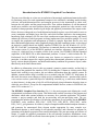
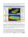


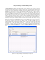
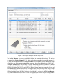
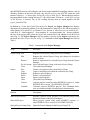
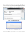
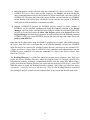

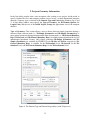
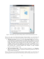
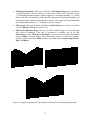
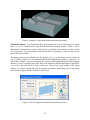
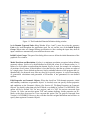

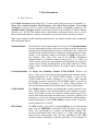
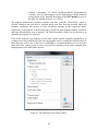

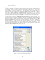
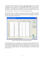
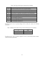
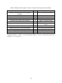
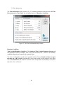
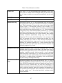
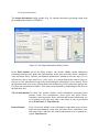
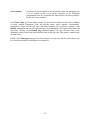
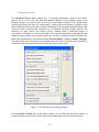
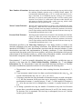
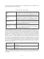
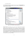
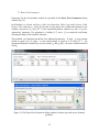
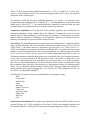
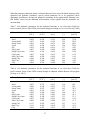
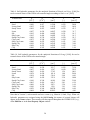
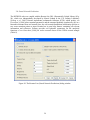
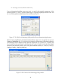
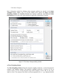
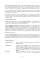
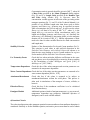
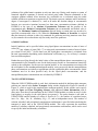
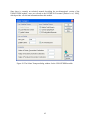
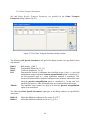
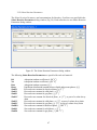
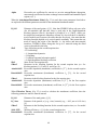
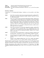

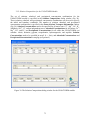
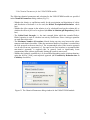
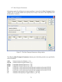
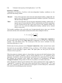
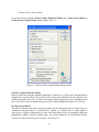
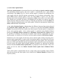
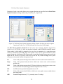
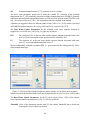
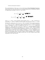
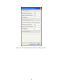
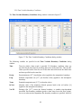

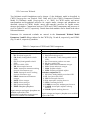
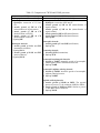
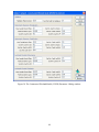
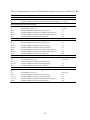
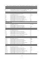
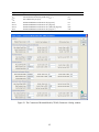
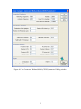
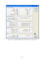
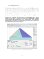
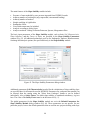
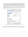
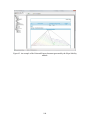
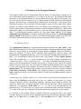
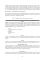
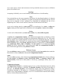
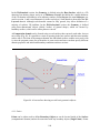
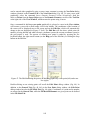
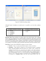
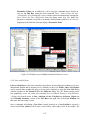
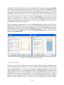
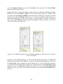
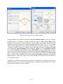
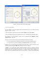
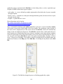
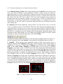
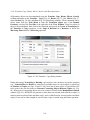
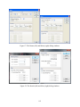
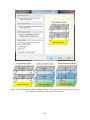
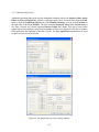
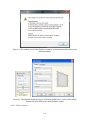
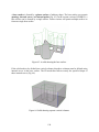
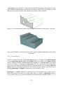
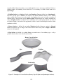
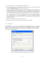
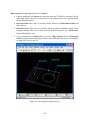
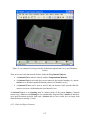
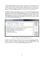
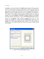
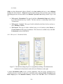
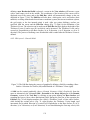
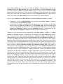
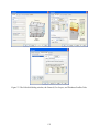
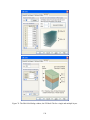
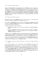
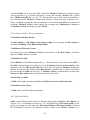
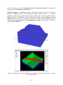
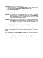
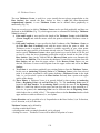
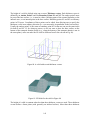
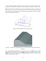
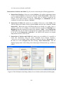
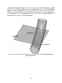
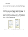
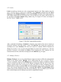
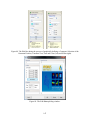
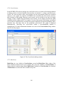
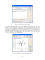
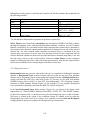
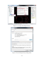
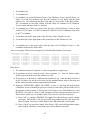

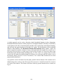
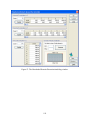
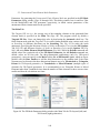
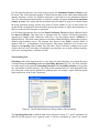
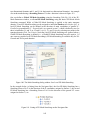
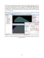
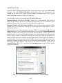
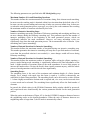
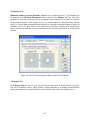
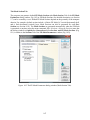
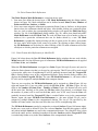

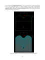
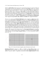
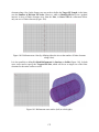
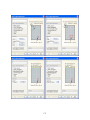
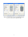
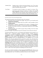
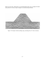
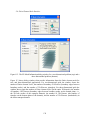
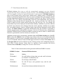
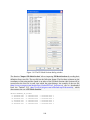

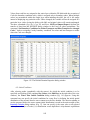
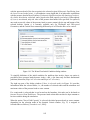
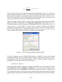
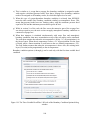
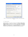
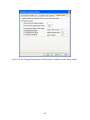
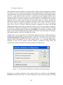
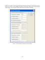
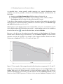
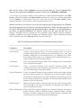
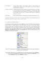
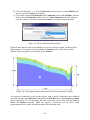
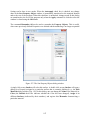
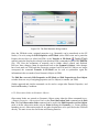
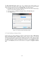
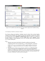
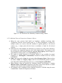
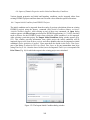
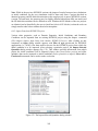
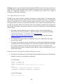
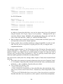
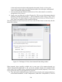
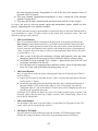

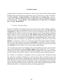
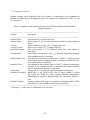
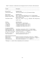
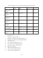
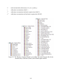
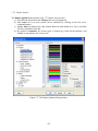
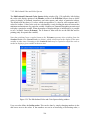
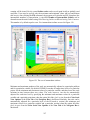
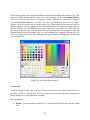
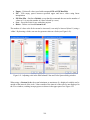

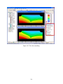
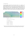
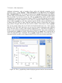
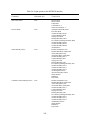
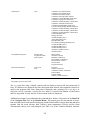
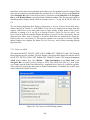
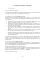
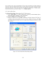
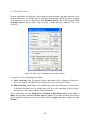
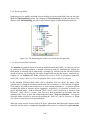
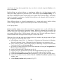
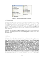
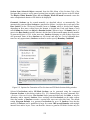
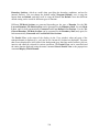
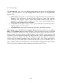
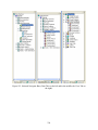
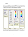
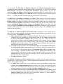
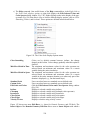
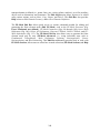
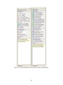
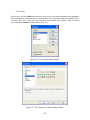
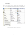
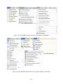
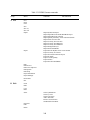


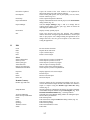
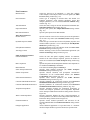
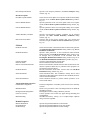
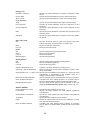


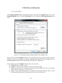
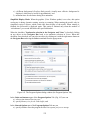
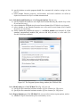
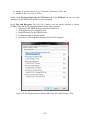
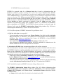
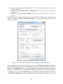
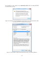
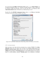
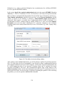
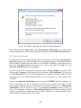
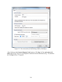
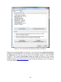
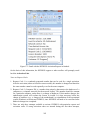
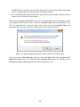
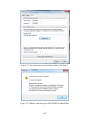
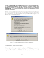
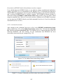
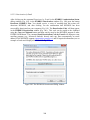
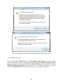
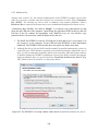

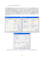
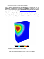
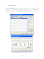
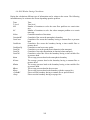
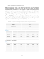
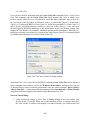
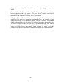
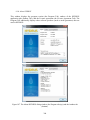


![User Manual [5.5 Mb - pdf]](http://vs1.manualzilla.com/store/data/005950654_1-5f0c3bfbdc0fa52796e7d9a416391587-150x150.png)