1
Version 3.1
March 1993
Program by
David L. Swofford
User's Manual by
David L. Swofford
and
Douglas P. Begle
Laboratory of Molecular Systematics
MRC 534, MSC
Smithsonian Institution
Washington DC 20560
USA
Development of versions prior to 3.1 supported by
Center for Biodiversity
Illinois Natural History Survey
607 E. Peabody Drive
Champaign, Illinois 61820
USA
License Agreement and Disclaimer
PAUP is licensed to individual users for the sole purpose of facilitating the
scientific research of the licensee. This software may be used in more than one
location or by more than one person provided that there is no possibility that it
will be used by two or more people simultaneously. Generally, this qualification
means either of the following: (1) the program may be used by a single
researcher on any number of machines in his or her possession, or (2) the
program may be installed on a single machine and used by one or more
individuals who have access to that machine.
If you cannot abide by the terms of this agreement, please return the software to
the Illinois Natural History Survey immediately for a refund of the distribution
fee.
THIS SOFTWARE IS PROVIDED "AS IS" WITHOUT WARRANTY OF ANY KIND. DAVID L.
SWOFFORD, THE SMITHSONIAN INSTITUTION, THE ILLINOIS NATURAL HISTORY SURVEY,
AND THE UNIVERSITY OF ILLINOIS DO NOT WARRANT, GUARANTEE, OR MAKE ANY
REPRESENTATIONS REGARDING THE USE OR THE RESULTS OF THE SOFTWARE OR
DOCUMENTATION IN TERMS OF THEIR CORRECTNESS, RELIABILITY, CURRENTNESS, OR
OTHERWISE. IN NO CASE WILL THESE PARTIES BE LIABLE FOR ANY SPECIAL, INCIDENTAL,
CONSEQUENTIAL, OR OTHER DAMAGES THAT MAY RESULT FROM USE OF THIS SOFTWARE.
Suggested Citation
PAUP 3.1 is in many ways comparable to a monographic article. In its over
70,000 lines of code, PAUP implements numerous original concepts and ideas
and contains many new algorithms. For these reasons, citation of the program in
a book format is recommended:
Swofford, D. L. 1991. PAUP: Phylogenetic Analysis Using
Parsimony, Version 3.1 Computer program distributed by the
Illinois Natural History Survey, Champaign, Illinois.
Copyright © Illinois Natural History Survey, 1989.
Copyright © Smithsonian Institution, 1993.
All Rights Reserved.
Apple, ImageWriter, LaserWriter, and Macintosh are registered trademarks of
Apple Computer, Inc. Finder and Multifinder are trademarks of Apple Computer,
Inc. Helvetica is a registered trademark of Linotype company. Microsoft is a
registered trademark of Microsoft Corporation. IBM is a registered trademark of
International Business Machines, Inc. Other brand and product names are
trademarks or registered trademarks of their respective holders.
Table of Contents
PRELIMINARIES
Acknowledgments........................................................................i
About This Manual ......................................................................ii
Organization.....................................................................ii
Typographical and notational conventions ......................iii
Why read the manual?......................................................v
Technical Support ........................................................................v
Anonymous FTP Server for PAUP Support ................................vi
CHAPTER 1
BACKGROUND .................................................1
General Concepts .........................................................................1
Tree Terms ...................................................................................4
Character Types ...........................................................................6
Ordered (Wagner) Characters ..........................................7
Unordered Characters ......................................................8
Dollo Characters ..............................................................8
Rooted vs. unrooted Dollo models.......................8
Polarity specification............................................12
Irreversible Characters .....................................................12
Polarity specification............................................12
User-Defined Character Types.........................................13
Character-state trees.............................................13
Stepmatrices.........................................................15
Tree Lengths and Character Weights...........................................18
Character-State Optimization.......................................................19
Missing Data ................................................................................21
Outgroups, Ancestors, and Roots.................................................24
Searching for Optimal Trees........................................................27
Exact methods..................................................................28
Exhaustive search.................................................28
Branch-and-bound algorithm ...............................29
Heuristic Methods............................................................32
Stepwise Addition................................................32
Branch swapping..................................................36
Searching under Topological Constraints........................40
"Monophyly" constraint trees ..............................40
"Backbone" constraint trees .................................43
Heuristic Searches and "converse"
constraints ............................................................44
Keeping "Near-Minimal" Trees .......................................44
Zero-Length Branches and Polytomies........................................45
Tree-to-Tree Distances.................................................................48
Consensus Trees...........................................................................50
Strict Consensus...............................................................51
Semistrict Consensus .......................................................52
Majority-rule consensus...................................................52
Adams Consensus ............................................................52
Consensus indices ............................................................53
Goodness-of-Fit Statistics............................................................54
A Posteriori Character Weighting................................................55
The "Bootstrap"............................................................................56
Lake's Method of Invariants.........................................................56
Pseudorandom Number Generation.............................................57
CHAPTER 2
USING PAUP .........................................................................................59
Input files .....................................................................................59
The NEXUS Format.........................................................59
Blocks...................................................................60
NEXUS file identification....................................60
General format of NEXUS files...........................61
The DATA Block.............................................................61
Entering the matrix in "transposed" format .........63
Placing taxon and character names ......................63
Character-state symbols .......................................64
Using alphanumeric character names ..................65
Predefined formats for molecular sequence
data.......................................................................66
Matching the states in the first taxon ...................67
Alignment gaps ....................................................68
EQUATE macros .................................................69
Using a subset of the characters...........................70
The Assumptions Block...................................................71
The TREES Block............................................................72
TAXA and CHARACTERS Blocks ................................73
"PAUP" Blocks................................................................74
Batch Processing..............................................................75
Error Messages and Input Files........................................76
Specifying Character Types.........................................................78
The "Standard" Character Types......................................78
Assigning Character Polarities.............................78
Defining Your Own Character Types ..............................79
Character-state trees.............................................79
Stepmatrices.........................................................82
Verifying USERTYPE definitions.......................83
Assigning Character Types ..............................................84
Character Weighting ....................................................................85
Assigning Weights ...........................................................85
Excluding Characters .......................................................87
Successive weighting .......................................................88
Defining Ancestral States.............................................................88
Defining and Using Outgroups ....................................................90
Simplifying Input with "Sets"......................................................91
Character Sets ("CHARSETs")........................................91
Taxon Sets ("TAXSETs")................................................92
Assumption Sets...............................................................93
Type sets ("TYPESETs").....................................93
Weight sets (WTSETs) ........................................93
Exclusion sets (EXSETs).....................................94
Invoking assumption sets.....................................94
Multistate Taxa ............................................................................95
Deleting and Restoring Taxa........................................................97
Distance Matrices.........................................................................98
Searching for Trees ......................................................................99
Heuristic Searches............................................................100
Branch-and-Bound Search ...............................................104
Exhaustive Search............................................................105
Lake's Method of Linear Invariants .................................107
Assessing Confidence using Bootstrap Analysis.............112
Random Trees ..................................................................115
Diagnosing Trees .........................................................................117
"Cladograms" and "Phylograms".....................................117
Consistency Indices and Goodness-of-Fit Statistics ........118
Table of Branch Lengths and Linkages ...........................118
Change and Apomorphy Lists..........................................119
Character Diagnostics ......................................................121
Character-State Reconstructions......................................122
Stepmatrix Character Reconstruction: Special
Considerations..................................................................124
The Pairwise Homoplasy and Patristic Distance
Matrices............................................................................128
Lengths and Fit Measures ............................................................129
Manipulating Trees ......................................................................131
Rooting Trees for Output and Character Diagnosis.........131
Saving Trees to Files........................................................133
Recovering Trees from Files............................................134
Comparing Trees..............................................................136
Calculating Consensus Trees ...........................................137
Filtering Trees..................................................................138
Condensing Trees.............................................................140
Rooting and Derooting Trees...........................................140
Printing and Plotting Trees ..............................................141
Changing the Order of Taxa on Trees..............................142
User-Defined Trees..........................................................143
Defining and Using Topological Constraints...............................146
Importing and Exporting Trees and Data.....................................149
Examining Current Status ............................................................152
Data Matrix ......................................................................152
Character Status ...............................................................152
User-Defined Character Types.........................................153
Ancestral States (ANCSTATES).....................................153
Tree Status........................................................................154
CHAPTER 3
COMMAND REFERENCE..................................................................155
Command Format ........................................................................155
Identifiers .........................................................................156
Taxon identifiers ..................................................157
Character identifiers.............................................157
Other names .........................................................158
Common Command Elements .........................................158
Taxon lists............................................................158
Character lists.......................................................158
Character states ....................................................159
Tree lists...............................................................159
Commands used in the Data Block..............................................159
CHARLABELS ...............................................................159
DIMENSIONS.................................................................160
FORMAT.........................................................................160
MATRIX..........................................................................162
OPTIONS.........................................................................162
STATELABELS ..............................................................163
TAXLABELS ..................................................................164
Commands used in the ASSUMPTIONS Block..........................164
ANCSTATES...................................................................164
CHARSET .......................................................................165
EXSET .............................................................................165
OPTIONS.........................................................................165
TYPESET.........................................................................166
USERTYPE .....................................................................166
WTSET ............................................................................166
Commands used in the TREES Block .........................................167
TRANSLATE ..................................................................167
TREE, UTREE.................................................................167
PAUP Commands ........................................................................168
Options Affecting Multiple Commands...........................168
Tree-searching options.........................................168
Tree-rooting options.............................................169
Tree output options ..............................................170
Options for character-matrix listings ...................170
Other options........................................................171
?........................................................................................171
! ........................................................................................171
ALLTREES......................................................................171
ANCSTATES...................................................................173
ASSUME .........................................................................173
BANDB............................................................................173
BOOTSTRAP ..................................................................174
CHARSET .......................................................................175
CHGPLOT .......................................................................175
CONDENSE ....................................................................176
CONSTRAINTS ..............................................................176
CONTREE .......................................................................177
CSTATUS........................................................................179
CTYPE.............................................................................179
DEFAULTS .....................................................................179
DELETE...........................................................................180
DEROOT .........................................................................181
DESCRIBE ......................................................................181
DOS..................................................................................183
EDIT.................................................................................183
EXCLUDE.......................................................................183
EXECUTE .......................................................................184
EXSET .............................................................................184
FILTER ............................................................................184
GETTREES......................................................................185
HELP................................................................................187
HSEARCH.......................................................................187
INCLUDE ........................................................................190
INGROUP........................................................................190
LAKE...............................................................................191
LEAVE.............................................................................192
LENFIT............................................................................192
LOG .................................................................................193
MEMAVAIL....................................................................194
OUTGROUP....................................................................194
POSSPLOT ......................................................................195
QUIT ................................................................................195
RANDTREES ..................................................................196
RESTORE........................................................................196
REVFILTER ....................................................................197
REWEIGHT.....................................................................197
ROOT...............................................................................197
SAVEASSUM .................................................................198
SAVETREES...................................................................198
SET...................................................................................199
SHOWANC .....................................................................203
SHOWCONSTR ..............................................................203
SHOWDIST.....................................................................203
SHOWMATRIX ..............................................................204
SHOWTREES..................................................................204
SHOWUSER....................................................................204
TAXSET ..........................................................................204
TREEDIST.......................................................................205
TREEINFO ......................................................................205
TSTATUS ........................................................................205
TYPESET.........................................................................205
USERTREE .....................................................................205
USERTYPE .....................................................................206
WEIGHTS........................................................................206
WTS .................................................................................206
WTSET ............................................................................206
CHAPTER 4
THE MACINTOSH INTERFACE ......................................................207
Installation....................................................................................207
The PAUP Editor .........................................................................207
The Command Line .....................................................................208
Selecting Items in Lists................................................................209
Running under MultiFinder® (or System 7.0 and Later) ............209
The Apple ( ) Menu....................................................................210
The File Menu..............................................................................211
New ..................................................................................211
Open….............................................................................211
Close.................................................................................212
Save..................................................................................212
Save As… ........................................................................212
Revert...............................................................................212
Page Setup…....................................................................213
Print File….......................................................................213
Echo to Printer .................................................................214
Print Selection..................................................................214
Log Output to Disk… ......................................................214
Execute (File)...................................................................215
Export File…....................................................................215
Import File…....................................................................216
Quit...................................................................................218
The Edit Menu .............................................................................218
Undo.................................................................................218
Cut....................................................................................218
Copy.................................................................................218
Paste .................................................................................218
Clear.................................................................................219
Select All..........................................................................219
Clear Display Buffer ........................................................219
Edit Display Buffer ..........................................................219
Set Tabs and Font.............................................................219
Find ..................................................................................219
Find Again........................................................................219
Replace.............................................................................220
Replace All.......................................................................220
The Windows Menu.....................................................................220
Main Display....................................................................220
Show Command Line.......................................................220
Show Memory Status.......................................................221
Search Status....................................................................221
PAUP Help.......................................................................221
Zoom ................................................................................221
Clean Up ..........................................................................221
Close All ..........................................................................222
Editor windows ................................................................222
The Options Menu .......................................................................222
Multistate Taxa… ............................................................222
Optimization….................................................................223
Set Maxtrees….................................................................223
Character Matrix Format…..............................................224
Searching…......................................................................225
Rooting….........................................................................225
Tree Order…....................................................................226
Stepmatrices….................................................................226
Ignore Characters… .........................................................227
Semigraphics…................................................................227
Editor…............................................................................228
Warnings & Errors….......................................................228
NEXUS Format…............................................................229
Startup Preferences… ......................................................230
Restore Option Settings… ...............................................230
The Data Menu.............................................................................231
Include-Exclude Characters… .........................................231
Set Character Types… .....................................................232
Set Character Weights…..................................................233
Reweight Characters… ....................................................234
Delete-Restore Taxa….....................................................234
Define Outgroup… ..........................................................235
Show Character Status .....................................................235
Show Taxon Status...........................................................236
Show Usertypes................................................................236
Show Data Matrix ............................................................236
Show Distance Matrix......................................................236
Show Ancestral States......................................................236
Choose Assumption Sets…..............................................236
The Search Menu .........................................................................237
Load Constraints… ..........................................................237
Show Constraints… .........................................................238
Heuristic….......................................................................239
Branch and Bound…........................................................241
Exhaustive…....................................................................242
Lake's Invariants… ..........................................................243
Bootstrap… ......................................................................243
Random Trees… ..............................................................244
The Trees Menu ...........................................................................245
Tree Info...........................................................................245
Clear Trees .......................................................................245
Condense Trees…............................................................245
Root Trees…/Deroot Trees…..........................................246
Tree-to-Tree Distances….................................................247
Lengths and Fit Measures… ............................................247
Filter Trees… ...................................................................248
Remove Filter...................................................................249
Reverse Filter ...................................................................249
Show Trees…...................................................................249
Describe Trees…..............................................................249
Show Reconstructions…..................................................250
Print Trees…....................................................................251
Compute Consensus….....................................................253
Print Consensus…............................................................254
Get Trees from File…......................................................254
Save Trees to File….........................................................256
REFERENCES.......................................................................................259
PRELIMINARIES
This manual is for version 3.1 of PAUP for the Apple Macintosh. It also
serves as preliminary documentation for the IBM-PC and "Portable"
(mainframe and workstation) releases of Version 3, which as of this
writing have still not been released. The manual is not as polished as I had
hoped it would be at this point. Hopefully, the weaker sections will be
enhanced by the time version 3.2 is released. I apologize for not including
an index. The manual is still evolving too rapidly at this point to justify
the considerable amount of time that indexing would require. Please
report any errors or other significant omissions.
Unfortunately, I have not yet been able to incorporate all of the many
useful features that users of PAUP have requested. I will continue to plug
away on the depressingly long "wish list". The most significant new
feature that I did not get working in time for this release are Archie-FaithCranston permutation/randomization tests (PTP, T-PTP). Randomization
tests will almost certainly be included in the next release. You're welcome
to check the anonymous FTP server (see below) for test versions
containing these and other new features, but of course I can make no
promises as to when these test versions will be made available.
David L. Swofford
28 March, 1993
ACKNOWLEDGMENTS
The number of people who have had a significant impact on the
development of PAUP continues to grow, and I must apologize for failing
to mention everyone who has suggested features or provided assistance. I
am especially grateful to Julian Humphries, an important source of useful
ideas and expertise during the development of earlier versions. It was
through Julian's prodding and assistance that the first interactive
mainframe version of PAUP was developed. He initially convinced me to
port the program to microcomputers and was instrumental in the
development of the first IBM PC version.
PAUP 3.1 USER'S MANUAL
i
Several of the newer features of PAUP have been heavily influenced by
many hours of lively discussion with David and Wayne Maddison and by
their truly outstanding program "MacClade." David served as a consultant
during the early stages of development of the Macintosh version of PAUP
and has patiently provided advice, assistance, and testing throughout the
development of PAUP Version 3. In addition to countless ideas for
interface and documentation improvements, David suggested significant
improvements in tree filtering (filtering by constraints), stepwise taxon
addition (random-addition-sequence enhancements), and tree-file
operations (most importantly, the use of Boolean operations for combining
trees in memory with trees in a file). Wayne was also heavily involved in
the testing and made many additional suggestions for improvements,
including introducing me to the notion of user-defined character types and
sharing algorithms for dealing with multistate taxa. I have also benefited
tremendously from discussions with Joe Felsenstein, particularly with
respect to the branch-and-bound algorithm. The unselfishness of these
individuals (who, after all, have a vested interest in the advancement of
their own programs) is a constant source of inspiration to me.
Many other individuals have reported bugs, made helpful suggestions
and/or provided stimulating ideas. These include Larry Abele, Vic Albert,
Jim Archie, Paul Berti, David Cannatella, Jonathan Coddington, Joel
Cracraft, Mike Cummings, Chris Darling, Scott Davis, Ron DeBry, Doug
Eernisse, Bill Fink, George Gutman, David Hillis, Kent Holsinger, Bob
Jansen, Rick Mayden, Chris Meacham, David Mindell, Mike Miyamoto,
Gavin Naylor, Mark Norell, David Penny, Norman Platnick, Winston
Ponder, Andrew Simons, Greg Spicer, Beth Stewart, Sherman Suiter,
David Stock, Rytas Vilgalys, and Jim Woolley.
Three members of the staff of the Illinois Natural History Survey, where
all previous versions of PAUP have been developed, deserve special
recognition. Angie Young has cheerfully and conscientiously taken care
of the day-to-day distribution matters and Mary Lou Williamson has
flawlessly kept the financial matters in order. Larry Page, director of the
Center for Biodiversity, provided encouragement and support throughout
the development of earlier versions.
Finally, I thank my wife, Ruth Swofford, for enduring many lonely
evenings while I wrote and debugged code and for willingly and
unselfishly providing assistance in many phases of the development of
PAUP.
ii
PAUP 3.1 User's Manual
ABOUT THIS MANUAL
Organization
The manual is divided into four chapters, the first three of which are
common to all implementations of PAUP. The first chapter presents
background material relevant to the capabilities of the program. We urge
all users to become familiar with this material before using the program.
Chapter 2 provides basic instruction on the use of PAUP's primary
functions and other features. Chapter 3 provides a detailed reference to
PAUP commands and input file organization. Chapter 4 is specific to
each implementation (i.e., Macintosh, Unix, etc.), and describes details of
the user interface that are specific to that implementation.
Typically, you will refer to Chapter 2 to find out what PAUP can do and
get a general idea of how to do it. When you need more specific
information, you will then refer to Chapters 3 and/or 4. Admittedly, this
organization is not ideal. From a user's point of view, it would be much
nicer if, for example, the instructions for using the menu/dialog-box
interface for setting character types were presented at the same time that
the equivalent command-based method was described. Unfortunately,
maintaining n different copies of the manual for n different
implementations would then become a nightmare from our point of view.
By isolating the implementation-specific portion of the manual in a single
chapter, we only need to maintain a single version of the remainder of the
manual.
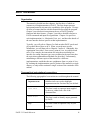
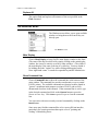
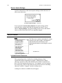
Typographical and notational conventions
The following typographical conventions are used throughout the manual:
Important term
Boldface italics are used to highlight
important terms the first time they are defined.
USER INPUT
This font is used to represent input supplied
by the user, either from a file or the
command-line.
PAUP output
This font is used to identify output generated
by PAUP.
Key
This font is used to represent a key on your
keyboard.
PAUP 3.1 USER'S MANUAL
iii
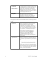
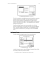
COMMAND
Menu Command
Dialog item
Command names are shown in boldface type.
Commands that are used from input files or
typed on the command line are indicated
using all upper-case characters. Commands
available for selection from menus are shown
in mixed upper and lower case.
This font is used to refer to buttons,
checkboxes, and other items contained in
dialog boxes or elsewhere on the screen.
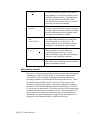
In descriptions of data-file and command formats, the following notation
is used:
ITEMTEXT
Items typed entirely in uppercase are to be
entered as indicated. Input of PAUP
commands is case-insensitive, however, so
you may enter command names, keywords,
etc., in any combination of upper- and lowercase characters. In addition, PAUP allows
abbreviations of command names and
keywords to the shortest unambiguous
truncation. Note that other NEXUSconforming programs (MacClade, in
particular; see below) may not accept these
abbreviations.
[ Optional-item]
Brackets around an item means that the item
is optional. Square brackets may be nested as
in
[OptionalItem [AnotherOptionalItem]]
In this case, each level of nesting depends on
the specification of the item at the next higher
level. You should not include these brackets
when you enter the command.
iv
PAUP 3.1 User's Manual
{A|B}
Two or more items enclosed in curly braces
and separated by vertical bars indicate a set of
mutually exclusive choices. The underlined
item (if any) indicates the default setting.
You should not include the braces or vertical
bar when you enter the command.
variable
Letters, words, and symbols shown entirely in
lowercase italics represent variables for which
specific information must be supplied by the
user when the command is entered.
item …
<item1 item2>…
An ellipsis indicates that the preceding item
may be repeated one or more times. If a
group of items may be repeated sequentially,
the group is surrounded by angle brackets.
[ ] { } … |
These symbols are used to define the
command format (see above). Unless
otherwise indicated, they should not be typed
when the actual command is entered.
; : . , " ' ( )
Other punctuation should be entered as shown
in the command description.
Why read the manual?
Many users of microcomputer software take the position that the manual is
something you refer to as a last resort. It is sometimes suggested that
"well-written" software largely eliminates the need for a manual by
providing an intuitive, menu-based interface that guides the user. While
this idealized state-of-affairs may be strictly true with respect to the
mechanics of running the program, a thorough reading of the manual is
essential in order to understand many of the biological aspects of PAUP.
If you do not read the manual, you will have no way of discovering many
useful features and shortcuts available in PAUP. More importantly, you
may be unaware of assumptions that the program is making during its
calculations. We cannot emphasize strongly enough the importance of
reading the User's Manual carefully, painful as this may be.
PAUP 3.1 USER'S MANUAL
v
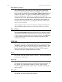
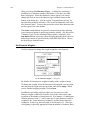
TECHNICAL SUPPORT
Assistance with the use of PAUP and interpretation of output will be
provided only to licensed users. If you are unable to resolve a problem by
experimentation or need information that is not available in the User's
Manual, you may reach me in any of the following ways:
E-mail:
[email protected]
(Internet)
Standard Mail:
David L. Swofford
Laboratory of Molecular Systematics
MRC 534, MSC
Smithsonian Institution
Washington, DC 20560
USA
Express courier: David L. Swofford
Laboratory of Molecular Systematics
Smithsonian Institution Museum Support Center
410 Silver Hill Road
Silver Hill Road
Suitland, Maryland 20746
FAX:
response)
(301)238-3059 (Note that I cannot guarantee a FAXed
Use of e-mail is vastly more likely to generate a quick response than the
other methods.
Please provide the following information in your communication.
1.
The exact wording of any error messages that you have received.
2.
If a crash occurred, the sequence of events prior to the crash (e.g.,
commands issued, etc.).
3.
The exact version number of your program. You can obtain the
version number from the opening screen that is displayed when
you first start the program.
4.
A copy of your data file.
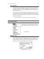
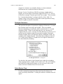
ANONYMOUS FTP SERVER FOR PAUP SUPPORT
We have set up an FTP server to support PAUP. We will periodically post
updated programs, test versions, documentation files, and other
announcements there. To use the FTP server, log in to onyx.si.edu
vi
PAUP 3.1 User's Manual
(160.111.64.54) as "anonymous" and enter your e-mail address when
prompted for a password. The overall structure of the ftp directories is
described in a README file in the root directory.
When minor bug-fix releases are issued, we will post an "updater"
program that will convert any version of PAUP/Mac 3.1 to the new
version. The updater program will only work if you already have a copy
of PAUP 3.1.
PAUP 3.1 USER'S MANUAL
vii
PAUP 3.1 USER'S MANUAL
1
Chapter
BACKGROUND
1
This chapter provides general background on the concepts underlying the
methods used in PAUP. Specific information on how to use the program
follows in later chapters.
GENERAL CONCEPTS
PAUP is a program for inferring phylogenies from discrete-character data
under the principle of maximum parsimony. Parsimony methods search
for minimum-length trees:1 trees that minimize the amount of
evolutionary change needed to explain the available data under a
prespecified set of constraints upon permissible character changes. The
best known discrete-character parsimony method, often called Wagner
parsimony (Kluge and Farris, 1969; Farris, 1970) treats binary or ordered
multistate characters and permits free irreversibility. Multistate characters
may also be left unordered (i.e., any character state is permitted to
transform directly into any other state), sometimes called Fitch parsimony
after Fitch (1971). Other parsimony variants place additional restrictions
on the types of character-state changes that are allowed. Dollo parsimony
(Farris, 1977) permits each derived, or apomorphic, character state to
originate only once. Camin-Sokal parsimony (Camin and Sokal, 1965)
prohibits reversals from a derived state to a relatively more ancestral, or
plesiomorphic, condition. Also introduced with version 3.0 of PAUP is a
1Some
authors (e.g., Wiley, 1979; Nelson and Platnick, 1981) prefer to distinguish
between the terms tree—a hierarchical statement regarding genealogical (ancestordescendant and sister-group) relationships—and cladogram—a branching diagram
depicting patterns of character distribution or nested sets of synapomorphies. This
distinction is purely terminological and probably inappropriate (Hendy and Penny, 1984).
PAUP may be used to construct to construct either trees or cladograms, the only
difference being how the user interpets the output. "Tree" will be used to refer to both
evolutionary trees and cladograms thoughout this manual, with apologies to those who
find this usage unacceptable.
2
PAUP 3.1 USER'S MANUAL
procedure based on the work of David Sankoff and his collaborators
(Sankoff and Rousseau, 1975; Sankoff and Cedergren, 1983) that allows
the user to specify the cost associated with a change from each character
state to each other state. Each of these methods is discussed in more detail
under "Character Types."
Minimization of the total tree length is equivalent to seeking trees that
imply the least amount of homoplasy, or similarity not directly attributable
to common ancestry. Homoplasies or "extra steps"—reversals,
parallelisms, and convergences—constitute ad hoc assumptions required
to bring observations into conformity with the "simpler" explanation that
possession of the same character state in two or more taxa is due solely to
inheritance from a common ancestor. A word about the relationship
between computerized minimum-length-tree approaches and the manual
methods used in traditional cladistics [e.g., Hennig (1966); Wiley (1981)]
is in order. The latter ("Hennigian") methods place a heavy emphasis on a
priori assessment of character polarity, the specification of which of the
observed character states represents the ancestral condition in the group
under study. If character polarities could always be reliably assessed, and
if there were no homoplasy in the data, then phylogeny reconstruction
would amount to nothing more than grouping taxa according to shared
derived character states (synapomorphies), with no relevance being
attached to the sharing of ancestral states (symplesiomorphies). That is,
all of the taxa that possess a particular derived character state could
unambiguously be interpreted as descendants of the ancestor in which the
state originated and taxa sharing the ancestral condition could be
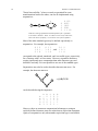
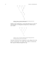
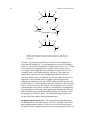
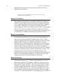
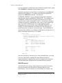
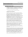
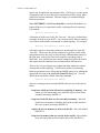
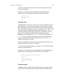
definitively excluded from that group. Inevitably, however, character
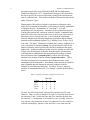
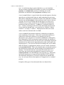
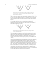
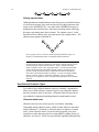
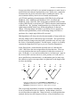
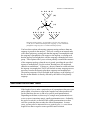
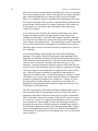
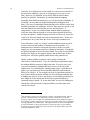
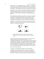
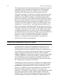
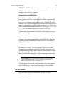
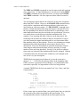
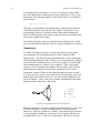
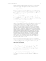
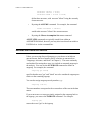
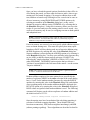
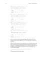
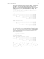
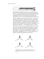
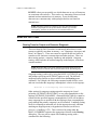
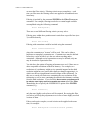
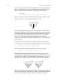
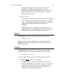
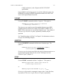
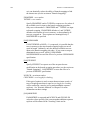
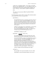
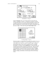
conflicts or incompatibilities arise. For example, consider the data shown
below:
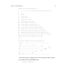
Table 1. Hypothetical data for example discussed in text.
Taxon
One
Two
Three
Four
1
1
1
0
0
Character
2
3
1
1
0
1
1
0
0
0
4
1
1
1
0
For now, we will assume that 0 represents the ancestral state for each
character. Thus, we observe that taxa One and Two share the derived state
for characters 1 and 3, while taxa One and Three share the derived state
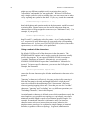
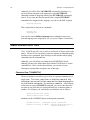
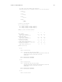
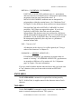
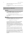
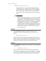
for character 2. Consequently, if One and Two were, in reality, sister taxa
(tree A below), the possession of state 1 for character 2 in One and Three
would be a homoplasy, whereas if One and Three were sister taxa, the
PAUP 3.1 USER'S MANUAL
3
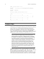
+
2(1)
+
1(1)
3(1)
2(1)
+
+
1(1)
3(1)
+ 1(1)
+ 3(1)
2(1)
4(1)
Tree A
Tw
o
Th
re
e
O
ne
Th
re
e
Tw
o
O
ne
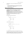
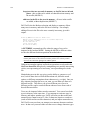
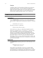
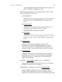
derived characters 1 and 3 shared by One and Two would be homoplasies
(tree B below)2
4(1)
Tree B
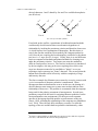
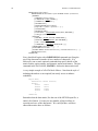
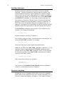
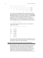
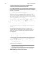
Two trees for the data of Table 1.
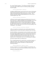
Faced with such a conflict, a practitioner of traditional manual methods
would usually decide between these two alternative hypotheses of
relationship by invoking the parsimony criterion and therefore choose tree
A, which requires fewer assumptions of homoplasy. But this choice is
exactly the one that would have been made by the computer method as
well, since the tree requiring the least homoplasy would also be the shorter
tree (tree A = 5 steps; tree B = 6 steps). Clearly, there is no real difference
between computerized methods and manual methods for choosing trees
under the parsimony criterion. Two factors can cause the methods to
differ in actual practice, however. The first lies in subjectivity introduced
by the investigator, who may prefer a tree requiring two or three extra
steps in a character assumed to be unreliable or "plastic" over a tree
requiring a single extra step in a "better" character. The second is that the
human brain is unable to deal effectively with the complexity of large
and/or noisy data sets.
The above example also illustrates one reason why excessive concern with
a priori assessment of character polarities is unwarranted. When
incongruent character distributions occur as in this case, the sharing of a
derived character state among two or more taxa need not indicate close
relationship of those taxa. The problem is accentuated when the outgroup
being used for the polarity assessment is heterogeneous. In such cases,
parsimony can provide the basis for assigning character polarities, but the
most parsimonious state assignment(s) for the most recent common
ancestor of the ingroup depends upon the overall structure of the tree
(Farris, 1982), including the relationships of the outgroup taxa (Maddison
et al., 1984). Thus, the only fully satisfactory recourse is to infer the
topology of the tree and the character polarities simultaneously, rather
2Of
course, a third possibility is that neither One and Two nor One and Three represent
sister taxa, with all shared derived states being homoplasies.
4
PAUP 3.1 USER'S MANUAL
than going through the two-stage process of assigning polarities first and
then estimating the tree.
NOTE: The concepts of character order and character polarity are often
confused. The former defines the nature of permitted character-state
transformations, whereas the latter refers to the direction of character evolution.
Specifying how character states are ordered with respect to each other is not the
same as determining which character state is ancestral.
For further amplification of these points, see the sections entitled "Character
Types" and "Outgroups, Ancestors, and Roots" later in this chapter.
TREE T ERMS
The most general terminology for describing the various components of
trees is derived from the field of graph theory [e.g., Harary (1969); Gould
(1988)]. Some of this terminology is reviewed briefly here, although
formalism is minimized. A graph consists of a set of vertices and a set of
edges, where each edge is a line joining a pair of vertices. Two distinct
vertices are adjacent if they are joined by an edge; the edge is said to be
incident to those vertices. The degree of a vertex is the number of edges
with which the vertex is incident. A path is a sequence of distinct edges
such that each edge shares one vertex in common with the preceding edge
in the sequence and the other vertex in common with the next edge in the
sequence. A path connecting a pair of vertices can also be described as a
sequence of vertices, with each vertex adjacent to the preceding vertex in
the sequence. A graph is connected if there is at least one path from any
vertex to any other vertex. A cycle is a path that connects a vertex to itself
in which no vertex is repeated. Most importantly for our purposes here, a
tree is a connected acyclic graph.
Vertices and edges on trees are often called nodes and branches,
respectively, and this terminology will be used throughout the manual.
Nodes are called terminal nodes if they have degree one and internal
nodes otherwise. Unfortunately, the above terminology is not
standardized, and much synonymy exists. Terminal nodes are also called
tips or leaves; branches (edges) are also called links, segments, intervals,
or internodes. Terminal nodes corresponding to biological taxa are often
called Operational Taxonomic Units (OTUs) or simply terminal taxa.
Similarly, internal nodes are sometimes referred to as Hypothetical
Taxonomic Units (HTUs) or hypothetical ancestors.
A tree is binary if none of its internal nodes has degree exceeding three. If
a binary tree has at most one vertex of degree two, it is also full. Full
binary trees are sometimes called strictly bifurcating or fully dichotomous
PAUP 3.1 USER'S MANUAL
5
trees. A node having degree greater than three (e.g., one immediate
ancestor and three immediate descendants; see below) corresponds to a
polytomy or a multifurcation, and trees containing one or more
polytomies are sometimes called polytomous (nonbinary) trees.
A tree is rooted if there is a special node (the root) that imparts a direction
upon the tree such that nodes lying on a path connecting the root to any
other node are ancestors of (ancestral to) nodes in the path that are further
from the root and descendants of (descendant to) nodes closer to the root.
Typically, the root is an internal node having degree two, however in
PAUP the root is usually considered to be an additional terminal node
positioned at the base of the tree. A subtree is a connected subset of a
tree. A subtree consisting of all of the nodes and branches that descend
from a particular internal node v on a rooted tree is called the "subtree
rooted at v" or simply "v's subtree." Phylogeneticists often refer to the
subtree rooted at an internal node as a clade.
A tree is ordered if the branches incident to each node are assigned in
some nonarbitrary (fixed) order. If the order in which the branches are
connected is irrelevant or arbitrary (as is generally the case for
phylogenetic trees), then the tree is said to be unordered. (Although the
trees computed by PAUP are unordered in the sense that free rotation of
subtrees around internal nodes does not affect the relationships implied for
terminal taxa, an order may be imposed based on other criteria purely for
output purposes.) Trees are also classified according to the way in which
nodes are labeled. In phylogenetic analysis, trees are usually considered
to be terminally labeled. That is, the terminal nodes correspond exactly to
the biological taxa under study, but the labeling of the internal nodes is
arbitrary. If all internal nodes are associated with actual objects (e.g.,
fossil taxa) and are not merely hypothetical constructs, the trees are
completely labeled. Note that although some programs (e.g., MacClade)
may permit actual taxa to occupy ancestral positions, PAUP considers
only terminally labeled trees; if a taxon is assigned to an internal node
(e.g., in a user-specified tree description) it is "popped out" to a terminal
position.
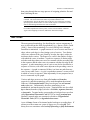
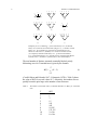
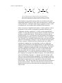
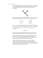
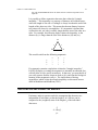
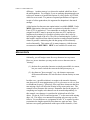
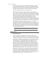
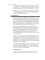
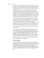
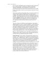
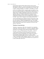
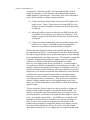
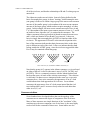
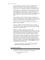
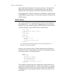
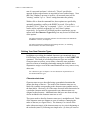
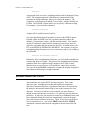
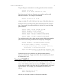
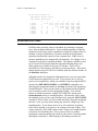
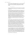
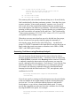
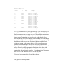
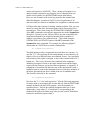
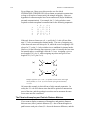
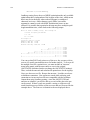
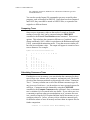
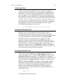
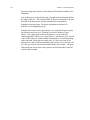
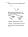
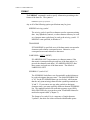
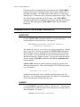
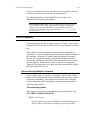
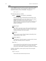
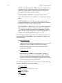
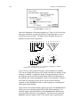
Examples of the types of trees discussed above are shown below.
6
PAUP 3.1 USER'S MANUAL
A
B
C
D
E
C
B
A
D
E
C
A
D
B
E
(a)
A
B
C
(b)
D
E
A
B
C
(c)
D
F
E
A
H
G
D
B
C
E
I
(d)
A
B
C
R
(e)
D
E
A
B
C
(f)
D
E
A
B
C
F
D
E
H
G
I
R
(g)
(h)
(i)
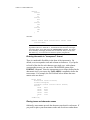
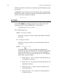
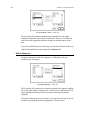
Examples for tree terminology. (a) Unrooted binary tree. (b) Rooted
binary tree (rooted at an internal node of degree 2), (c) Another rooted
binary tree. Trees b and c are equivalent as unordered trees but
distinct as ordered trees. (d) Binary tree rooted at terminal taxon R.
(e) Completely labeled rooted binary tree. (f) Unrooted nonbinary
tree. (g) Rooted nonbinary tree. (h) Path between terminal nodes B and
D (heavy lines). (h) Subtree of node G (heavy lines and boldface).
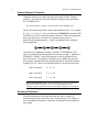
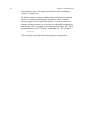
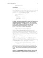
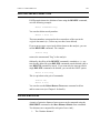
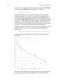
The total number of distinct, unrooted, terminally labeled, strictly
bifurcating, trees for T terminal taxa is given by the formula
T
B(T) =
∏ (2i – 5)
(1)
i=3
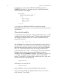
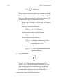
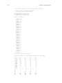
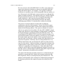
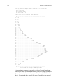
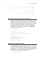
(Cavalli-Sforza and Edwards, 1967; Felsenstein, 1978b). Table 2 shows
the value of B(T) for several values of T. Obviously, the number of trees
quickly becomes quite large as the number of taxa increases.
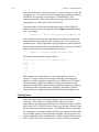
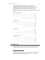
Table 2.
The number of unrooted, binary, terminally labeled trees, B(T), for T terminal
taxa.
T
B(T)
3
4
5
6
7
8
9
10
15
1
3
15
105
945
10,395
135,135
2 x 10⁶
8 x 10¹²
PAUP 3.1 USER'S MANUAL
7
20
50
2 x 10²⁰
3 x 1074
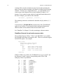
CHARACTER T YPES
PAUP implements different parsimony variants through the declaration of
a character type for each character included in the data matrix. Available
types are ordered (Wagner), unordered (Fitch), Dollo, irreversible
(Camin-Sokal), and user-defined. Any combination of character types
can be assigned to the characters in the data matrix. The character types
(and weights) that are specified constitute the a priori assumptions that are
in effect for a particular analysis.
Character types may be classified as either undirected or directed. An
undirected character is one in which for every pair of states a and b, the
"cost" in tree length is the same for the transformations A→B and B→A.
All of the standard character types are undirected except for irreversible.
Stepmatrix characters (defined below) are undirected if and only if the
stepmatrix is symmetric, i.e., dij = dji for all pairs of character states i,j (see
below). The "directedness" of the characters bears a close relationship to
whether PAUP stores trees as rooted or unrooted trees. When directed
characters are in effect, trees must be treated as rooted trees, because the
position of the root may affect the length of the tree. On the other hand, if
all characters are undirected, PAUP ordinarily considers the trees to be
unrooted, since the length of the trees is independent of the position of the
root. Unrooted trees need not be explicitly rooted before requesting
subsequent output. PAUP roots trees automatically using the currently
defined outgroup (or via Lundberg rooting) whenever necessary.
In addition, characters are either polarized or unpolarized. Polarized
characters are those for which the state ancestral to all other states is
prespecified. If the ancestral state is not specified or is designated as
"missing," the character is said to be unpolarized. 3
A character type may formally be described as a weighted directed graph
(weighted digraph). The vertices of the graph correspond to character
states, and the edges of the graph are arrows corresponding to permissible
character-state changes. The weight of each edge is the "cost" associated
with the transformation from one character state to another.
3Unfortunately,
this terminology is unstandardized. Meacham (1984) and others use
"directed" vs. "undirected" in the same sense that I use "polarized" vs. "unpolarized". My
usage of "directed" is more consistent with graph theoretic concepts (see next paragraph).
8
PAUP 3.1 USER'S MANUAL
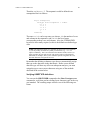
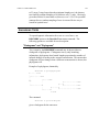
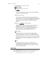
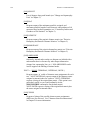
Ordered (Wagner) Characters
"Ordered" characters are those typically associated with the "Wagner
method." The character states are ordered according to their position in
the "SYMBOLS list."
See "The Data Block" (Chapter 2) for information on the SYMBOLS list.
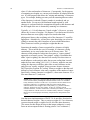
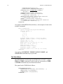
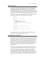
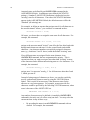
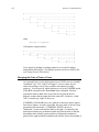
The list of symbols represents a linear transformation series. For example,
if symbols="ABCDE" were specified in the FORMAT command of the
DATA block, PAUP would treat ordered characters under the assumption
that to get from state A to state E, the character must proceed
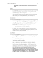
progressively through states B, C, and D, as indicated in the characterstate graph below:
A
1
B
1
C
1
D
1
E
No numerical or alphabetical order is assumed. If SYMBOLS="021",
state 2 is assumed to be intermediate between states 0 and 1. Similarly, if
SYMBOLS="ABQC", state B lies between A and Q, and state Q lies
between B and C. No polarity is implied by the symbols list, however.
For example, all of the following transformations are consistent with the
symbols list "012"; there is no requirement that '0' be the ancestral state:
state 0 ancestral:
0→1→2
state 1 ancestral:
2←1→0
state 2 ancestral:
2→1→0
Note to PAUP Version 2 Users: The default character type is now unordered,
rather than ordered as in earlier versions. Unless ordered characters are
explicitly requested, PAUP will assume that multistate characters are unordered.
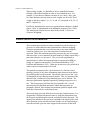
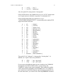
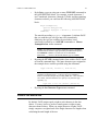
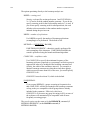
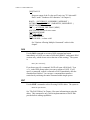
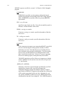
Unordered Characters
Unordered characters are defined such that any state is capable of
transforming directly to any other state, with equal cost. For example, a
five-state unordered character with states A through E has the characterstate graph:
PAUP 3.1 USER'S MANUAL
9
A
1
1
1
B
1
C
1
1 1
1
D
1
1
E
Character-state assignments are made to internal nodes of the tree so as to
minimize the total number of character-state transformations (steps), using
an algorithm based on that of Fitch (1971).
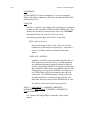
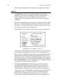
NOTE: The "ordered" vs. "unordered" concept does not pertain to binary
characters. The order of a character refers to the potential pathways of character
transformation, and there is only one possible path between the two states of a
binary character. Consequently, it makes no difference whether freely reversible
binary characters are defined as "ordered" or "unordered."
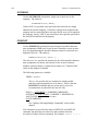
Dollo Characters
A "Dollo" character is one that is consistent with the requirement that
every derived character state be uniquely derived. If a hypothetical
ancestor is included in the analysis, this definition corresponds to the
traditional Dollo model in which each character state is allowed to
originate only once during evolution and all homoplasy takes the form of
reversals to a more ancestral condition (i.e., parallel gains of the derived
condition are not allowed).
As for ordered (Wagner) characters, character states are linearly ordered
according to their position in the symbols list specified in the FORMAT
command of the DATA block. However, we now define a "forward
transformation" as a change from a less derived state to a more derived
state, and a "backward transformation" as a change from a more derived
state to a less derived state.
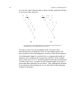
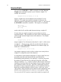
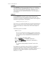
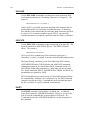
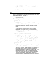
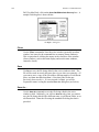
Rooted vs. unrooted Dollo models
PAUP (as well as MacClade) differs from some other implementations of
Dollo parsimony (e.g., Felsenstein's PHYLIP) in that it can operate as an
unrooted method. The only requirement is that the reconstructed character
states be consistent with the constraint that each derived state be uniquely
derived. Under this definition, the position of the root affects neither the
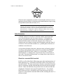
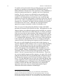
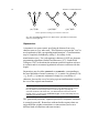
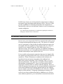
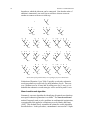
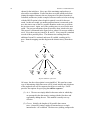
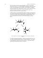
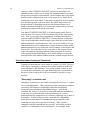
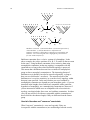
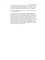
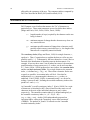
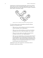
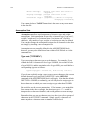
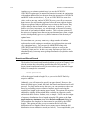
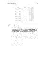
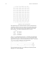
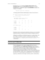
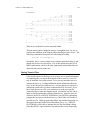
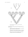
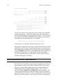
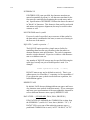
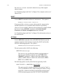
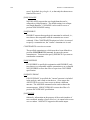
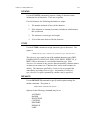
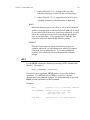
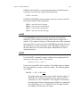
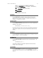
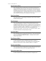
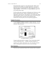
assignment of character states nor the length of the tree. For example,
both of the trees below, which differ only in the placement of the root,
require two steps under the unrooted Dollo model, assuming that state 1 is
the derived state:
10
PAUP 3.1 USER'S MANUAL
0
1
1
0
0
1
1
1
0
1
1
1
1
0
Reconstructions for a Dollo character under two different rootings of
an unrooted tree. Terminal taxa are labeled according to their state
for the character in question.
That is, neither tree requires more than a single origination of state 1. (In
the tree on the right, the derived state (1) is assumed to be ancestral with
respect to the group ABCD, but derived relative to some more inclusive
group.)
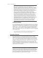
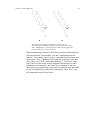
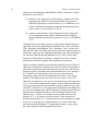
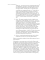
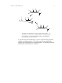
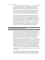
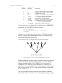
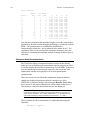
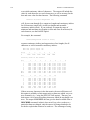
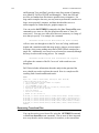
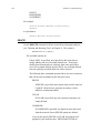
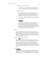
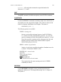
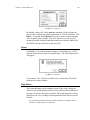
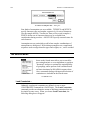
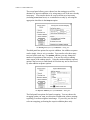
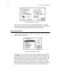
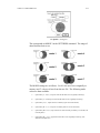
If, on the other hand, the trees are rooted by the attachment of a
hypothetical ancestor possessing state 0, the left tree will be shorter (2
steps) than the right tree (3 steps):
0
1
1
1
0
0
1
1
0
1
1
1
1
0
0
0
Reconstructions for a Dollo character on the trees of the figure above
under a rooted Dollo model.
The extra length in the right tree comes from the inclusion of the initial
gain of state 1 in the tree length. This example makes it clear that trees
computed under Dollo parsimony are intrinsically rooted only if we
assume we know the state at the "outgroup node" [sensu Maddison et al.
(1984)].
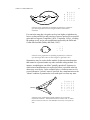
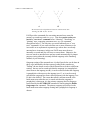
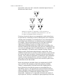
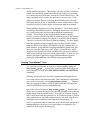
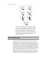
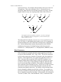
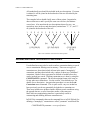
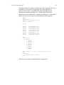
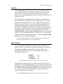
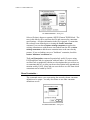
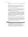
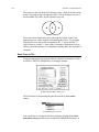
A more formal definition of the unrooted Dollo criterion is the following.
A character-state reconstruction satisfies the Dollo constraint if it is
possible to trace a path between any pair of nodes possessing the same
character state without passing through a node possessing a less derived
state. For example, reconstruction A below, while requiring fewer steps
than reconstruction B, is not a Dollo reconstruction, as tracing the path
connecting the two terminal nodes possessing state 1 requires passing
through internal nodes possessing the less derived state 0. Reconstruction
B, on the other hand, does satisfy the Dollo constraint.
PAUP 3.1 USER'S MANUAL
11
1
0
0
0
0
1
0
0
1
0
a
1
1
0
1
1
0
b
Two reconstructions for a single character on an unrooted tree.
Reconstruction a requires 2 steps but violates the Dollo constraint.
Reconstruction b satisfies the Dollo constraint, but requires 3 steps.
Note that there is no possible rooting of the tree which does not require
independent (parallel) gains of state 1 under reconstruction A, whereas any
rooting of the tree is consistent with a unique origination of state 1 under
reconstruction B, in accordance with traditional Dollo parsimony.
Unless an ancestor is included in the analysis—either explicitly or due to
the presence of irreversible or asymmetric stepmatrix characters (see
"Outgroups, Ancestors, and Roots")—PAUP uses the unrooted Dollo
method. If, on the other hand, an ancestral taxon is included, then PAUP
performs a rooted Dollo analysis. (If all characters are binary and are
assigned polarity "up," as noted below, the rooted analysis corresponds to
the implementation of Dollo parsimony in PHYLIP.) Since tree lengths
will, in general, vary according to the position of the root, the result of the
analysis is an intrinsically rooted tree—any specification of outgroups by
the user is ignored. While the ability to obtain rooted trees without
assuming an outgroup may seem appealing, it comes at a high price.
Suppose a derived character state appears both in our ingroup and in an
undisputed outgroup taxon also included in the data matrix. The analysis
will place a premium on making all of the taxa possessing the derived
state a monophyletic group (subject, of course, to effects from other
characters in the data set), since the alternative is likely to be many
independent losses. As a result, taxa that would ordinarily be assigned to
the "outgroup" may spring from within the ingroup. Even when no basis
exists for identifying "outgroup" vs. "ingroup" taxa, the rooting is still
likely to be more artifactual than meaningful. The assumption is that the
ancestor of the full tree possesses the ancestral state for the character and
that the derived states must evolve somewhere on the tree from this
ancestral state. Thus, the tree tends to be rooted nearest the taxa that have
the fewest derived states. This may in fact be what you want, but you
should at least be aware of the reasons why the program places the root
where it does.
12
PAUP 3.1 USER'S MANUAL
To amplify on the points made in the preceding paragraph, note that Dollo
parsimony is sometimes recommended for restriction site data [e.g.,
DeBry and Slade (1985)] because of the asymmetry in the probabilities of
losing an existing restriction site vs. gaining a new site at a particular
location. (If a site is present, any substitution at any position in the
recognition sequence causes a site loss, whereas even if a particular
sequence is one substitution away from being a site, exactly the right
substitution at exactly the right position is required to convert the "one-off
site" to a site.) Thus, a rooted Dollo analysis in which the ancestral state is
assumed to be "site absent" will tend to root the resulting tree(s) near the
taxa that have the fewest sites. Although one could argue that this
approach to rooting is reasonable, it seems a bit arbitrary to me.
There are ways of circumventing the problems of using rooted Dollo
parsimony for characters like restriction site data. One approach is to infer
character polarity via traditional outgroup analysis and then use a mixture
of Dollo and Camin-Sokal (irreversible characters, see below) parsimony.
If the site occurs only in (some) members of the ingroup, then we would
designate the ancestral state as "absent" and allow a single gain of the site
followed by as many losses as would be required to explain the character
(i.e., traditional Dollo parsimony). But if a site occurs in the ingroup and
in the outgroup, the assumption that the site was already present in the
common ancestor of the ingroup-plus-outgroup would be reasonable. In
this case, we would designate the ancestral state for this character as
"present" and then treat the character as an irreversible (rather than Dollo)
character, allowing only losses of the site in accordance with the Dollo
model. A somewhat simpler but logically equivalent approach is to
constrain the ingroup to be monophyletic (either through the use of a
heavily weighted "dummy" synapomorphy or by using the "topological
constraints" feature of PAUP) and use Dollo parsimony with an "allabsent" ("all-zero") ancestral taxon for all of the characters. Then if the
site occurs in both the ingroup and the outgroup, a site gain will be forced
along the basal branch of the tree (terminating at the common ancestor of
the ingroup-plus-outgroup) and all subsequent character changes will be
losses. If, on the other hand, the site occurs only within the ingroup, then
a single origination will be assigned within the ingroup, perhaps with one
or more subsequent losses.4 Fortunately, the unrooted Dollo approach
available in PAUP and MacClade renders these more complicated
approaches unnecessary, but users should understand the logical
connections between the alternative methodologies.
4An
"all-missing" ancestor with polarity "up" [see "Direction of transformations
(polarity)]" for all characters could also be used, with equivalent results. The same
character state would be assigned to the node corresponding to the common ancestor of
the ingroup-plus-outgroup in either case. The only difference is that with an all-absent
PAUP 3.1 USER'S MANUAL
13
NOTE: Felsenstein (1984) has described a variation on rooted Dollo analysis
that he calls the "unordered Dollo" method. (This terminology is a bit
unfortunate—"unpolarized" Dollo would have been a better name.) Unlike the
Dollo method implemented in PAUP, which assumes that the polarity is known,
the unpolarized Dollo method evaluates each character on a given tree under all
possible polarity assignments and chooses that polarity which allows the
minimum number of changes. For example, in a two-state character with states
0 and 1, we would count first the number of changes required under the
assumption that state 0 is ancestral, and then count the number of changes
required under the assumption that state 1 is ancestral. Polarity is then assigned
in accordance with the assignment requiring the fewest changes. I cannot
imagine a situation in which one would be willing to assume that a character
could not evolve from an ancestral state to a derived state more than once, but
unwilling to postulate the character's polarity. Consequently, PAUP does not
implement this method. (If you can imagine such a situation, let me know.) The
unpolarized Dollo approach is not appropriate for restriction site data, since
allowing site presence to be ancestral and site absence to be derived would,
under the Dollo model, imply that sites could only be lost once and then
regained as many times as necessary, clearly an unreasonable assumption.
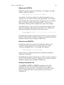
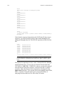
Polarity specification
For the unrooted Dollo method, PAUP allows either the lowest or highest
observed state (as defined by the SYMBOLS list) to be the ancestral state
(polarity "up" vs. "down," respectively). If you do not explicitly specify
"up" or "down," "up" is assumed. When an ancestor is included in the
analysis (rooted Dollo), any state in the SYMBOLS list may be designated
as the ancestral state.
See Assigning Character Polarities under "Specifying Character Types" in
Chapter 2 for information on how to designate character polarities.
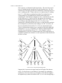
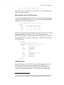
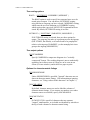
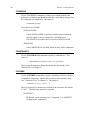
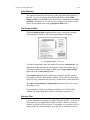
Irreversible Characters
Irreversible characters are equivalent to ordered characters with the
additional constraint of irreversibility being imposed (Camin and Sokal,
1965). As for ordered (Wagner) characters, character states are linearly
ordered according to their position in the SYMBOLS list specified in the
FORMAT command of the DATA block. However, we now prohibit
transformations from a more derived state to a less derived state. For
example, if SYMBOLS="ABCDE" and state A is defined as the ancestral
state, the character-state graph is:
(all-zero) ancestor, one step would be added to the tree length for every character in
which the site was present in both the ingroup and outgroup, corresponding to the site
gain along the basal branch. With an "all-missing" (unknown) ancestor, this additional
step would not be required, because the change would be from the "missing" state to
present (see "MISSING DATA"). Thus, the only difference between the two methods is
that a constant is added to (or subtracted from) the tree length.
14
PAUP 3.1 USER'S MANUAL
A
1
1
B
1
C
D
1
E
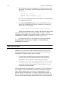
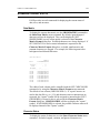
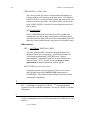
Polarity specification
Although character transformations must always proceed in the direction
of a more derived state, they need not proceed in a single direction with
respect to the SYMBOLS list. Any state in the SYMBOLS list may be
designated as the ancestral state; with states preceding and/or following
this state representing more derived states. For instance, state C could
instead have been chosen as the ancestral state in the example above. The
character-state graph would then be:
A
E
1
1
B
D
1
1
C
See Assigning Character Polarities under "Specifying Character Types" in
Chapter 2 for information on how to designate character polarities.
NOTE: Felsenstein (1984) has described a variation on irreversible-character
parsimony that he calls the "unordered Camin-Sokal" method (analogous to his
"unordered Dollo" method discussed above). Again, "unpolarized CaminSokal" would have been a more appropriate name. As in the unordered Dollo
method, the unpolarized Camin-Sokal method evaluates each character on a
given tree under all possible polarity assignments and chooses that polarity
which allows the minimum number of changes. It seems exceedingly unlikely
that one would be willing to assume that a character was irreversible, but
ignorant as to its polarity, so I have not implemented unpolarized irreversibility
in PAUP.
User-Defined Character Types
Two kinds of user-defined character types are available. Stepmatrices
allow you to define arbitrary character types by specifying the distance
from any character state to any other. Character-state trees provide an
easy method for inputting branching character transformation series.
Character-state trees
Character-state trees are used to specify a non-linear, branching,
relationship among character states, which are then otherwise treated as
ordered characters. (Formally, a character-state tree imposes a "partial
order" on the character states.) In most earlier programs, users were
required to recode character-state trees using additive coding (binary or
otherwise; see below). PAUP now provides this capability automatically.
PAUP 3.1 USER'S MANUAL
15
As an example, suppose that you wish to assume that states C and D were
derived independently from state B, which itself was derived from state A.
The following character-state tree would be used to represent this
relationship:
C
D
B
A
Either of the following additive codings, breaking the character into a suite
of independent characters, could be used in lieu of a character-state tree:
A
B
C
D
=
=
=
=
00
10
20
11
A
B
C
D
= 000
= 100
= 110
= 101
However, such a coding makes interpretation of the output more difficult
because you would have to decode the new characters back to the original
states of the character-state tree. In this case, the character-state tree
specification
((C,D)B)A
provides an equivalent definition of the character, requires essentially
identical computation time, and eliminates the coding-decoding steps.
Characters defined as character-state trees are fully reversible, however
they may evolve only along the paths specified by that definition. For
instance, in the above example a change from state C to state D would
imply passage through state B and would require two steps.
Finally, remember that character-state trees, like linearly ordered
characters, are undirected. The character-state tree only specifies
available paths for character-transformation; it does not imply anything
about polarity. In the example above, states B, C, or D could just as easily
have been placed at the base as shown below:
16
PAUP 3.1 USER'S MANUAL
A
C
D
A
D
B
B
A
C
B
C
(A,C,D)B
((A,D)B)C
D
((A,C)B)D
Three equivalent rootings of a character-state tree.
See "The ASSUMPTIONS block" for details on the specification of characterstate trees in an input file.
Stepmatrices
A stepmatrix is a square matrix specifying the distance from every
character state to every other state. These distances represent the "cost" in
tree-length units of the corresponding transformations. (Transformations
may be completely forbidden by coding 'i', for infinity, as the
transformation cost.) For each stepmatrix character, PAUP uses dynamic
programming algorithms (Sankoff and Rousseau, 1975; Sankoff and
Cedergren, 1983) to determine the minimum possible length on each tree
it evaluates and to reconstruct hypothetical ancestors consistent with this
length.
Stepmatrices may be either symmetric or asymmetric, corresponding to
the usual definition of matrix symmetry (i.e., a matrix d is symmetric if dij
= dji for all i,j). Symmetric stepmatrices imply free reversibility of
characters, because the cost of reversing a given transformation is equal to
the cost of the original transformation.
NOTE: Asymmetric stepmatrices force a rooted tree. If the stepmatrix is
asymmetrical, the taxon designated "ancestor" is very important. If you want to
have asymmetrical transition penalties but remain agnostic regarding the
ancestral condition of the characters, you should include an ancestor with allmissing values. See the section "Character Types" for the relationship between
character type and tree rooting.
The "generalized parsimony" approach provided by stepmatrix characters
is extremely powerful. Researchers with nucleotide sequence data can
assign different weights to transitions vs. transversions (and even to
different kinds of transitions and transversions):
PAUP 3.1 USER'S MANUAL
17
5
A
1
5
G
1
C
A
C
G
T
T
5
A
0
5
1
5
C
5
0
5
1
G
1
5
0
5
T
5
1
5
0
5
Character-state graph and corresponding stepmatrix for a character
type that assigns five times more weight to transversions than to
transitions
For restriction map data, site gains can be given higher weight than site
losses, so that parallel loss and gain-loss events are preferred over parallel
gains and loss-regains (Templeton, 1983b; Templeton, 1983a) , avoiding
the perhaps overly severe strict prohibitions imposed by the Dollo and
Camin-Sokal models (DeBry and Slade, 1985) :
3
+
+
1
- +
0 3
1 0
Character-state graph and corresponding stepmatrix for a character
type that assigns three times as much weight to a gain than a loss.
Stepmatrices may be used to define models of character transformation
that cannot be expressed under any other available coding method. For
instance, morphologists can define "partially unordered" characters in
which some transformations are required to follow a specified order but
others may occur freely. In the example below, a character-state tree for
several alternative "present" states is specified, but a transformation to the
"absent" condition is permitted to occur with equal cost from any state:
C
1
1
B
1
(absent)
0
1
1
A
1
1
0
A
B
C
D
0
0
1
1
1
1
A
1
0
1
2
1
B
2
1
0
1
2
C
3
2
1
0
3
D
2
1
2
3
0
D
Character-state graph and associated stepmatrix for a "partially
unordered" character. Transformations between states A, B, C, and D
follow a character-state tree, but immediate losses may occur from any
state.
18
PAUP 3.1 USER'S MANUAL
"Partial irreversibility," where reversals are permitted for some
transformations but not for others, can also be implemented using
stepmatrices:
1
0
1
1
1
2
0
1
2
3
3
0 123
0123
1012
2101
i i i0
Character-state graph and associated stepmatrix for a "partially
irreversible" character. State "3" cannot reverse to any other state,
hence the entries of infinity ("i") in the last row of the stepmatrix.
Most of the other standard types may be defined equivalently as
stepmatrices. For example, the stepmatrices
0 1 2
1 0 1 ,
2 1 0
0 1 1
1 0 1 , and
1 1 0
0 1 2
i 0 1
i i 0
correspond to the ordered, unordered, and irreversible types, respectively,
for a character with 3 or fewer states. However, stepmatrix characters
require significantly more computation than other character types and
should be used only if it is not possible to use one of the standard types.
Stepmatrices may also be used to describe character-state trees. For
example, the character-state tree
A
B
C
= ((A,B)C,E)D
E
D
can be described using the stepmatrix:
A
B
C
D
E
A
2
1
2
3
B
2
1
2
3
C
1
1
1
2
D
2
2
1
1
E
3
3
2
1
-
However, there are enormous computational advantages to using an
explicitly defined character-state tree rather than an equivalent stepmatrix.
Again, use stepmatrices only when another equivalent type is unavailable.
PAUP 3.1 USER'S MANUAL
19
See "The ASSUMPTIONS block" for details on how to define a stepmatrix in an
input file.
It is possible to define stepmatrix characters that violate the "triangle
inequality." This inequality is a property of distances in Euclidean space,
where the length of one side of a triangle is always less than the sum of the
lengths of the other two sides. This means the shortest distance between
two points will always be a straight line. If a stepmatrix is defined that
violates this rule, one side is actually longer than the sum of the other two
sides. For example, the following triplet violates the inequality, as the
distance (b,c) is longer than the sum of the distances (a,b) and (a,c).
a
1
b
1
c
4
This would result from the following stepmatrix:
a
b
c
a
1
1
b
1
1
c
1
4
-
If a stepmatrix contains a triplet that violates the "triangle inequality,"
PAUP will display a warning the stepmatrix is internally inconsistent, but
will still allow it to be used in an analysis. In that case, you must decide if
you really want to disallow shortcuts such as (bc), and what the biological
meaning of that stepmatrix really is. The implications of having
stepmatrices which violate the triangle inequality are discussed in more
detail in Maddison and Maddison (1992).
TREE L ENGTHS AND CHARACTER WEIGHTS
Parsimony analysis operates under the assumption that characters are
independent of each other, so that the length L of a full tree can be
computed as the (weighted) sums of the lengths lj of the individual
characters:
C
L=
∑wjlj
j=1
,
20
PAUP 3.1 USER'S MANUAL
where C is the total number of characters. Consequently, for the purpose
of computing tree lengths, we can treat each character in isolation from the
rest. It is this property that allows the "mixing and matching" of character
types. For example, nothing prevents you from assuming that one subset
of the characters is ordered (Wagner), another is unordered, and yet
another Dollo. For any tree, the minimum length required by each
character is evaluated under the assumptions assigned to that character and
the full length of the tree is obtained by summing over characters.
Typically, wj = 1 for all characters ("equal weights"). However, you may
choose any vector w of weights. For instance, if you had reason to believe
that two characters were tightly coupled for reasons other than
phylogenetic history, then weighting each of the characters 1/2 would be
appropriate. Alternatively, you may have prior knowledge (or at least be
willing to assume) that some characters are more reliable than others.
These characters could be given higher weight than the rest.
Sometimes the number of states recognized for a character is highly
arbitrary. This would be the case, for example, if a character varying
continuously in size were broken into a set of discrete states. The
character could perhaps be broken into four states (a "course-grained"
approach) or ten states (a more "fine-grained" coding). Remember that
under "equal weighting" the character will actually have three times as
much influence on the analysis under the ten-state coding than it would
under the four-state coding [(10-1)/(4-1)]. Likewise, under the ten-state
coding, the character would have nine times as much influence on the
analysis as an "equally weighted" binary presence-absence character.
PAUP provides an option for "scaling" character weights so that the total
influence of each character is the same, regardless of the number of states.
Specifically, a binary character is weighted 1, a three-state character 1/2, a
four-state character 1/3, and so on.
NOTE: Some workers have suggested that the problem of the above paragraph
can be circumvented by breaking the multistate character into a set of additive
binary characters, but this is not the case. If you break a ten-state character into
nine binary characters, it is indeed true that each of the resulting binary
characters has the same weight as does a truly binary (e.g., presence-absence)
character, but there are now nine of them. In fact, for a linearly ordered
multistate character, it makes no difference to the analysis whether you treat it as
a single character or break it into a set of additive binary characters. Doing the
latter serves no useful purpose and merely complicates the interpretation of the
output.
Note that most implementations of PAUP 3.0 do not allow fractional or
decimal character weights. Thus, to assign a weight of 1/2 to a character,
you must instead assign a weight of two to all of the other characters.
(The reason for this design decision is that integer arithmetic is vastly
faster on microcomputers than is floating-point or "real" arithmetic.)
PAUP 3.1 USER'S MANUAL
21
When scaling weights, it is desirable to choose a smallest common
multiple of the desired weights in order to avoid roundoff error. For
example, if your data set contains a mixture of two-, three-, four-, and
five-state characters and you want to scale weights, use 60 as the "base"
weight so that the weights 1/2, 1/3, 1/4, and 1/5 correspond to 30, 20, 15,
and 12, respectively.
PAUP also implements the successive approximations character method
(Farris, 1969) as implemented in the Hennig86 program (Farris, 1988).
This method is discussed in more detail in the section "A Posteriori
Character Weighting."
CHARACTER-STATE OPTIMIZATION
The reconstruction of character states at internal (ancestral) nodes on a
given tree is called character-state optimization or character mapping.
Character optimization does not come into play at any time during the
search for optimal trees; only when character reconstructions are
requested. Under the maximum parsimony criterion, the goal is to assign
character states so as to minimize the total number of change required by a
particular character on a given tree. The set of such assignments at
internal nodes is called a most-parsimonious reconstruction (MPR) or
simply an "optimal reconstruction" (Swofford and Maddison, 1987;
Swofford and Maddison, 1992). Characters do not have to be polarized in
order for these reconstructions to be made.
The optimal reconstruction for a given character is a function of tree
topology, but also of any other assumptions about character order and/or
irreversibility that have been made. Specifically, this involves the "cost"
of changing from one character state to another. This is a function of the
character type, whether one of the standard types or user-defined. The
character optimization algorithm operates by making two passes over a
tree. The first pass proceeds from the tips toward the root. At each
internal node, the algorithm determines which character states are
potentially allowed, and calculates the minimum possible lengths of the
clade above that node for each allowed state.
The second stage proceeds from the root to the tips, and determines a set
of optimally reconstructed internal states by using the information from
the first pass and information from the second pass below that node. The
optimal state minimizes the sum of two quantities: the length of the clade
above that node given each allowed state and the cost of transforming to
each allowed state given the state assigned to the ancestor of that node.
22
PAUP 3.1 USER'S MANUAL
In most cases there will only be one optimal assignment at a node, but it is
possible that more than one optimum may exist. In that case, a particular
reconstruction may be favored on the basis of additional criteria. The
most common ancillary criteria are accelerated transformation
(ACCTRAN) and delayed transformation (DELTRAN) (Swofford and
Maddison, 1987; Maddison and Maddison, 1992; Swofford and
Maddison, 1992). Basically, these assign states at internal nodes in order
to delay (DELTRAN) or accelerate (ACCTRAN) character transformation
within the tree. By "pushing" transformations up or down the tree, these
optimization methods lead to very different hypotheses of character
change. Delaying change will lead to a preference for two origins of a
character state (parallelisms), while accelerating change will lead to a
preference for a single origin followed by reversal.
Both hypotheses will always involve the same number of steps on the tree.
The only change will be where those steps are located. The result will be
that the character change associated with a particular node will vary with
the choice of optimization method. For that reason, you have to carefully
examine the output that PAUP gives you (see Character Diagnostics).
In the figure below, assume that the ancestral state is 0, and that taxa
A,B,C, and D have the state assigned them for that character. There are
two ways that this character can be optimized: either the occurrence of
state 1 in B and C is a reversal (reconstruction a), in which case 1 arose at
the level of (ABC) and was lost in A; or the presence of 1 in B and C is
due to parallelism (reconstruction b), or independent gain. In either case,
this character requires two steps when it is optimized, so the length of the
tree does not change.
0
1
1
0
0
1
1
0
A
B
C
D
A
B
C
D
0->1
0->1
1->0
0->1
(a)
(b)
Character optimization using ACCTRAN and DELTRAN. (a)
ACCTRAN optimization of character with distribution shown. (b)
DELTRAN optimization of character. Both require two steps.
This is especially important if an analysis is explicitly examining the
levels of parallelism/reversal in a data set. In that instance, there are
several steps that one might take. Most obviously, use both optimization
methods, and see how the characters fall out—it may be that there is no
PAUP 3.1 USER'S MANUAL
23
difference. Another strategy is to choose the method which best favors
the null hypothesis. For example, if you are studying adaptation and want
to discover instances of parallel derivations of a trait, choose ACCTRAN,
which favors reversals. If a pattern of repeated parallelisms still appears
in spite of a bias against them, the argument for adaptation is that much
stronger.
A third option for character-state optimization is available: MINF. Under
MINF optimization, character states are optimized so that the f-value of
Farris (1972) is minimized. Two constraints are enforced: the states
assigned to an HTU must be present in at least one OTU, and the tree
length must be minimal (it is possible to further reduce the f-value by
increasing the length of the tree). The effect of minimizing the f-value is
that length is transferred from interior branches towards terminal branches
whenever possible, minimizing the risk that groups will be arbitrarily
resolved internally. This option will, in many instances, yield the same
reconstruction as DELTRAN. MINF is not available for rooted trees.
MISSING DATA
Ordinarily, you will assign a state for every character in every taxon.
However, in two situations you may need to score a character state as
"missing":
(1) the data for a particular character are simply unavailable in a taxon,
but you want to include the taxon in the analysis anyway, or
(2) the character "does not apply" (e.g., the character represents
different modifications of a structure that is absent entirely in some
taxa).
In either case, a possible solution is to assign to the taxon the character
state that would be most parsimonious given its placement on the tree (but
see Maddison (In press). Effectively, then, only those characters that have
non-missing values will affect the location of any taxon on the tree. The
example below illustrates this concept. Remember that for the purpose of
computing tree lengths, each character can be treated independently; in
this example, one character is considered in isolation from all of the
others. For tree A, PAUP would assign state "1" to the taxon with missing
data (=B). This allows a reconstruction requiring only one step over the
full tree. For tree B, however, assignment of state "0" is required in order
to minimize the length required by this character, again one step. Thus,
both trees are equally parsimonious with respect to this character; if one
24
PAUP 3.1 USER'S MANUAL
tree is in fact "better" than the other, evidence for this conclusion will have
to come from other characters.
A
1
B
?
\ / C
1
1
\ / D
1
0
\ / E
0
0
\ / F
0
0
\ /
0
\
0
G
A
B
D E
F
? 0 0 0
0
\ /
\ /
0
0
\
/ A
C
\ /
1
1
0
\ /
\
1
\
/
\ /
0
\
\
0
G
B
Demonstration of PAUP's handling of missing data. Reconstruction of
one character on two different trees (see text).
Note that in some cases, the assignment of the "would-be" most
parsimonious state is ambiguous. However, the length required is the
same regardless of how the ambiguity is resolved, so that for the purposes
of calculating the length of a particular tree or comparing the lengths of
alternative trees, ambiguity does not present a problem. In the example
below, either state "0" or "1" could be assigned to taxon B (reconstructions
A and B, respectively). In either case, the required length of two steps is
greater than that required by the trees above. Thus, although this character
is not informative for placing taxon B, it is still useful for discriminating
among tree topologies.
PAUP 3.1 USER'S MANUAL
D
0
25
E
0
D
0
\ / F
0
0
\ / A
0
1
\ / C
0
1
\ / B
0 ? 0
\ /
0
\
0
G
A
E
0
\ / F
0
0
\ / A
0
1
\ / C
1
1
\ / B
1 ? 1
\ /
1
\
0
G
B
Two equally parsimonious reconstructions on the same tree,
demonstrating the handling of ambiguity in the presence of missing
data. Although the two reconstructions are different, the length of the
reconstructions is two steps in each case.
When reconstructing characters, PAUP always assigns a nonmissing state
to all internal nodes. Occasionally, users have complained about this
behavior. For example, some users have argued that for the reconstruction
shown below, state '?' should have been assigned to the nodes at the base
of the {D,E} and {C,D,E} clades rather than state 1. This choice would
imply, however, that state 0 could be assigned to these nodes in a mostparsimonious reconstruction. But if state 0 were assigned to either of
these nodes, the reconstruction would require at least two steps rather than
the one step implied by the indicated reconstruction. Thus, state 1 is the
only permissible state for these nodes.
26
PAUP 3.1 USER'S MANUAL
A
1
B
1
\ /
1
\
C
?
\
D
?
E
?
\ /
1
\ /
\
1
\
/
\ / F
1
1
\ / G
1
0
\ /
0
\
0
H
\
A character-state reconstruction that illustrating the inappropriateness
of assigning missing values to internal nodes.
Similarly, in the example below, we must assign either state 1 or state 2 to
all internal nodes, even though non-missing states are defined only for
taxa A and B.
A
1
B
2
C
?
D
?
\ /
/
/
1
/
/
\ /
/
1
/
\ /
1
\
?
A character-state reconstruction that illustrating the inappropriateness
of assigning missing values to internal nodes.
Sometimes, internal-node state assignments are truly ambiguous due to the
presence of missing data. For example, either of the two reconstructions
below require the minimum length of one step:
PAUP 3.1 USER'S MANUAL
27
A
1
B
1
C
?
D
0
\ /
/
/
1
/
/
\ /
/
0
/
\ /
0
\
0
A
1
B
1
C
?
D
0
\ /
/
/
1
/
/
\ /
/
1
/
\ /
0
\
0
PAUP always chooses one of the potential reconstructions according to
the character types and optimization options in effect. However, it also
provides capabilities for examining all possible state assignments to
internal nodes so that you can determine whether or not a reconstruction
contains ambiguities.
See "Character-State Optimization" for information regarding the resolution of
ambiguity in character-state reconstructions.
OUTGROUPS, ANCESTORS , AND ROOTS
In most cases, trees computed by PAUP are unrooted and need be rooted
for output and interpretational purposes only. The absence of a defined
root is a consequence of the fact that for undirected character types, the
tree length is the same regardless of the position of the root. However,
rooted trees are computed when any of the following are true: (1)
characters of type "irreversible" are present; (2) asymmetric stepmatrix
characters are present; or (3) a hypothesized ancestral taxon is explicitly
included in the analysis at the request of the user.
For irreversible and asymmetric stepmatrix characters, the length of the
tree depends upon the position of the root, so the trees must be stored as
rooted trees. When all characters are undirected, the inclusion of a
hypothesized ancestral taxon corresponds to the traditional, but
unnecessary practice (Meacham, 1984; Meacham, 1986) of a priori
character polarization. This approach is reasonable when the polarity
determination is unambiguous (i.e., there is no heterogeneity in the
outgroup for characters that are variable within the ingroup). However,
when the outgroup is heterogeneous, the most parsimonious assignment of
an ancestral condition for the ingroup depends upon how the outgroup
taxa are related to each other [see Maddison et al. (1984) for a complete
analysis of this problem]. If outgroup relationships are already well
resolved, you can use methods described by Maddison et al. (1984) to
assess character polarities a priori and include an ancestral taxon in the
28
PAUP 3.1 USER'S MANUAL
analysis [see also Donoghue and Maddison (1986)]. Otherwise, it makes
much more sense either to:
(1) include several outgroup taxa in the analysis, with the root of the
ingroup portion of the tree being determined by the location at
which the outgroup taxa connect to the tree [i.e., Maddison et al.'s
(1984) "simultaneous resolution of ingroups and outgroups taken
to the extreme"; see also Farris (1972)], or
(2) compute an unrooted tree for the ingroup taxa only, making no a
priori assumptions about polarity, and then attach an outgroup
taxon (or hypothesized ancestor) to the tree a posteriori (Lundberg,
1972).
Although clearly better than "guessing" at the polarity, both of the above
approaches have some disadvantages (Maddison et al., 1984; Meacham,
1984; Donoghue and Maddison, 1986; Meacham, 1986). In order to be
fully effective, the first method requires the inclusion of characters that are
informative with respect to outgroup relationships even if these characters
are invariant within the ingroup (Maddison et al., 1984). On the other
hand, the second method can generate "optimal" trees that are locally
parsimonious within the ingroup, but not globally parsimonious.
If the trees being evaluated are rooted (either implicitly because directed
characters are present or explicitly due to the user's decision to include an
ancestral taxon), the character states taken by the ancestor of the full tree
must be specified. By default, these ancestral states are set to "missing" (=
the "standard" ancestor), however, the user may make alternative
assignments using ANCSTATES definitions (see below). The default
setting of all-missing values was chosen for two reasons. First, if all
characters are undirected, trees may be converted from rooted to unrooted
or vice versa with no change in tree length. Second, if directed characters
are present, the program has the freedom to assign a character-state to the
"first fork" of the tree (i.e., the internal node immediately descending from
the root corresponding to the initial branching event) that permits the most
parsimonious reconstruction subject to the constraints imposed by the
character type. Consider, for example, an irreversible character with
polarity "up." If, for whatever reason, the state for all terminal taxa
included in the analysis is "1," then the character will contribute no length
to the tree, as expected for a constant character (A, below) But if the
ancestral state had defaulted to "0" rather than "missing," a step would
have been assigned to the basal branch (B, below)
PAUP 3.1 USER'S MANUAL
29
1
1
1
\ /
/
1
/
\ /
1
\
?
A
1
1
1
\ /
/
1
/
\ /
1
\
0
B
Reconstruction for a hypothetical character with ancestral state
"missing" (a) and "0" (b). See text.
PAUP provides commands for converting unrooted trees stored in
memory to rooted trees and vice versa. Note that you do not have to
invoke a "root trees" command before "showing," "describing" or
"printing" trees, requesting consensus trees, etc. (see command
descriptions below). The only time you would ordinarily use a "root
trees" command is if you want to declare one or more characters to be
irreversible or an asymmetric stepmatrix type when there are already
unrooted trees in memory; in this case PAUP must store the trees
internally as rooted and you will have to convert them. Otherwise, the
trees are stored as unrooted trees and are rooted automatically for output
purposes (using either the currently defined outgroup or the Lundberg
method, at your choosing).
Outgroup rooting of the unrooted tree A in the figure below can be done in
three ways indicated by the three arrows leading to the rooted trees.
"Pulling" the tree down at each of the different arrows leads to a different
rooting: the tree can be rooted such that the outgroup is a monophyletic
sister-taxon to the ingroup (tree B); it can be rooted such that the outgroup
is paraphyletic with respect to the ingroup (tree C); or it can be rooted
such that the outgroup taxa form a basal polytomy with the ingroup (Tree
D; this is the default). The reason that taxon A and not taxon B is the
basal-most taxon when the tree is rooted such that the outgroup is
paraphyletic is that taxon A is the primary outgroup (the first outgroup
taxon listed by the OUTGROUP command or chosen using the Define
Outgroup menu command. The primary outgroup will always be the
basal-most taxon when outgroup rooting and a paraphyletic outgroup is
chosen.
30
PAUP 3.1 USER'S MANUAL
A
B C
D
E
( b)
B
C
D
( a)
A
A B
C
D
(c)
E
E
A B
C
D
E
( d)
Outgroup rooting options. (a) unrooted tree for five taxa, outgroup is
A + B. (b) tree rooted with monophyletic outgroup. (c) tree rooted with
paraphyletic outgroup. (d) tree rooted with basal polytomy.
You have three options when using outgroup rooting and more than one
outgroup is present in the analysis. These are: rooting at an internal node
with a basal polytomy; rooting such that the ingroup is monophyletic and
the outgroup is paraphyletic with respect to the ingroup; or rooting such
that the ingroup is monophyletic with the outgroup a monophyletic sister
group. These options allow you to at least partially constrain the structure
of the outgroup topology when the tree is rooted, providing the specified
ingroup is monophyletic. See the section "Rooting trees for output and
character reconstruction." If, however, the tree cannot be rooted such that
the ingroup is monophyletic, PAUP will include as many outgroup taxa as
necessary to make the ingroup plus those outgroup taxa monophyletic.
The primary outgroup is never included in the ingroup, so the topology of
the tree in that instance is directly affected by the choice of the primary
outgroup.
SEARCHING FOR OPTIMAL TREES
If the length of a tree under a particular set of assumptions (character types
and weights) is less than or equal to the length of any other possible tree
for the same data, the tree is said to be optimal (most parsimonious).
Depending on the data set, there may be a single most parsimonious tree
or two or more (sometimes many) equally parsimonious trees. Ordinarily,
the goal of a search is to find all of the equally parsimonious trees that
exist for a particular data set under the chosen assumptions. In some
cases, you may also be interested in near-optimal trees, i.e., trees whose
length is less than or equal to some specified cutoff criterion.
PAUP 3.1 USER'S MANUAL
31
PAUP provides two basic classes of methods for searching for optimal
trees, exact methods and heuristics. Exact methods guarantee to find the
optimal tree(s) but may require a prohibitive amount of computer time for
medium- to large-sized data sets. Heuristic methods do not guarantee
optimality but generally require far less computer time.
Note that the search algorithms described below consider only binary
trees. In many cases, however, the data will not be sufficient to determine
a fully resolved (i.e., binary) tree, however, so that branches of zero-length
might occur. In earlier versions of PAUP, two or more trees that could be
derived through different resolutions of polytomies were always
considered to represent distinct binary trees containing zero-length
branches, with the result that many more trees were sometimes saved than
was actually necessary. For example, if a tree contained two trichotomies,
nine equally parsimonious trees would be saved—three resolutions for the
first trichotomy times three resolutions for the second. Version 3 of
PAUP provides an option to collapse branches having zero length to yield
polytomies. Because two or more distinct binary trees may collapse to the
same nonbinary tree, the program then must ensure that after collapsing, a
tree does not become identical to a tree already saved that was obtained by
collapsing a different binary tree.
See "Zero-Length Branches" and Polytomies below for further details on this
point.
Exact methods
Exhaustive search
The conceptually simplest approach to the search for optimal trees is
simply to evaluate every possible tree. Assuming that exact methods exist
for evaluating the length of any particular tree, an algorithm that generates
all possible tree topologies and evaluates each one is guaranteed to find all
of the optimal trees. The algorithm outlined in the figure below can be
used for this purpose. Initially, the first three taxa in the data set are
connected to form the only possible unrooted tree for these taxa (row 1).
In the next step, the fourth taxon is added to each of the three branches of
the three-taxon tree, thereby generating all three possible unrooted trees
for the first four taxa (row 2). The process continues in a similar fashion,
adding the ith taxon to each branch of every tree (containing i–1 taxa)
generated during a previous step. Thus, for example, row 3 contains all 15
possible trees for the first five taxa, obtained by adding the fifth taxon to
each of the five possible branches for the three trees obtained at the fourtaxon stage. This process demonstrates the rationale for equation (1) for
counting the number of possible unrooted bifurcating trees for T taxa: for
each of the possible trees for i–1 taxa, there are 2(i–1) – 3 = 2i – 5
32
PAUP 3.1 USER'S MANUAL
branches to which the ith taxon can be connected. Note that the order of
addition is immaterial; one could just as well have chosen a taxon at
random to connect to the tree at each step.
B
C
1
A
B
D
B
D
C
B
C
C
D
2A
2B
2C
A
B
E
A
E
D
3A
C
C
D
E
E
3G
C
D
C
B
B
E
3I
3J
B
A
C
B
A
C E
D
B
C
E
D
3L
A
D
A
C
A
E
B
3K
C
3H
E
3E
A
D
A
D
D
3D
B
A
C
B
E
A
C
E
C
C
3C
A
B
3F
D E
C
3B
A
E D
B
E
C
B
D
B
D
B
B
A
D
D
3M
A
E
3N
A
3O
A
A
Generation of all possible binary tree topologies for five terminal taxa.
Evaluation of Equation 1 (see Table 2) quickly reveals why exhaustive
search procedures are useful only for small numbers of taxa. There are
over 2 million trees for 10 taxa and 34 million trees for 11 taxa, so it is
doubtful that exhaustive search strategies will be useful beyond 11 taxa.
Branch-and-bound algorithm
Fortunately, an exact algorithm for identifying all optimal trees that does
not require exhaustive generation is available. The branch-and-bound
method, frequently used to solve problems in combinatorial optimization,
was apparently first applied to evolutionary trees by Hendy and Penny
(1982). This method closely resembles the exhaustive search algorithm
described above. In this procedure, a search tree is traversed in a "depth-
PAUP 3.1 USER'S MANUAL
33
first" sequence, as illustrated in the figure below. The root of the search
tree (A) contains the only possible tree for the first three taxa. We first
construct one of the three possible trees obtained by connecting taxon 4 to
tree A, yielding tree B1. Then, to this tree, we connect taxon 5, yielding
tree C1.1. (If the data set contained more than five terminal taxa, we
would continue to join additional taxa in this manner until a tree
containing all T taxa had been completed.) Now, we backtrack one node
on the search tree (i.e., back to tree B1) and generate the second tree
resulting from the addition of taxon 5 to tree B1 (= tree C1.2). When all
five of the trees derivable from tree B1 (C1.1–C1.5) have been
constructed, we backtrack all the way to tree A of the search tree and take
the second path away from this node, leading to tree B2. As before, all
five trees derivable from tree B2 (C2.1–C2.5) are constructed in turn.
Then we backtrack once again to tree A and proceed down the third path
toward trees C3.1–C3.5. Eventually, we will have constructed all of the
possible trees culminating with tree C3.5. If the length of each tree
containing all five taxa were evaluated at the time of its construction, we
would have performed an exhaustive search equivalent to that described in
the above section.
B C
A
B
A
E
B
E
D
C
D
C
C1.1
A
E
A
D
B
B
B
D
C
C1.2
C
A
B D
E
C3.2
A
A
B C
E
B2
C
C
D
D
B D C
E
C1.3
B
C
B3
B1
A
C3.1
D
A
A
C3.3
A
B CE D
B DE C
C3.4
C1.4
A
B
A
D
B C
C
C1.5
E
E
A
D
B ED C D E
A
C2.1
E C
C
B
A
C2.2
B
D
D C
B
E
B
D C
C3.5
A
E
A
A
C2.3
C2.4
A
C2.5
Search tree for branch-and-bound algorithm.
Suppose that L represents an upper bound on the length of the shortest
tree(s). For the present, we can obtain L, for example, by evaluating a
random tree; if we know that a tree of length L exists, then the length of
the optimal tree(s) cannot exceed this value. If, as we are moving along a
34
PAUP 3.1 USER'S MANUAL
path of the search tree toward its tips (containing all T taxa), we encounter
a tree whose length exceeds L, then we need proceed no further along this
path; connecting additional taxa cannot possibly decrease the length.
Thus, we can dispense with the evaluation of all (phylogenetic) trees that
descend from this node in the search tree and immediately backtrack and
proceed down a different path. By cutting off portions of the search tree
in this manner, we can greatly reduce the number of trees that must
actually be evaluated.
If we reach the end of a path on the search tree and obtain a tree whose
length is less than or equal to the upper bound L, then this tree is a
candidate for optimality. If, however, this length is less than L, then this
tree is the best one found so far, and we have improved the upper bound
on the length of the optimal tree(s). This bound-improvement is important
because it may enable other search paths to be terminated more quickly.
When the entire search tree has been traversed, all optimal trees will have
been identified.
Several factors influence the running time of the branch-and-bound
algorithm. The quality of the data is perhaps the most important factor;
large data sets with little homoplasy will run quickly because most paths
of the search tree are terminated early. The speed with which the length of
each tree can be evaluated, a function of the character types, is also
important. In general, undirected character types run faster than directed
types because certain algorithmic tricks for rapidly computing tree lengths
can be used when the tree length does not depend on the location of the
root. Ordered (Wagner) characters are much faster than unordered
characters for similar reasons. User-defined stepmatrix characters, on the
other hand, run very slowly due to the enormous amount of computation
required to compute the length of even a single tree. Finally, of course,
the speed of the available computer is critical to the run times—the
branch-and-bound algorithm can be applied to larger data sets on a Cray
X/MP than on a Macintosh Plus.
The above presentation of the branch-and-bound method, while correct, is
an oversimplification of the algorithms actually used in PAUP, which
implements algorithmic refinements that greatly speed the computations.
These refinements, designed to promote earlier cut-offs in the traversal of
the search tree, include: (1) using heuristic methods (see below) to obtain
a near-optimal tree whose length is used as the initial upper bound; (2)
designing the search tree so that divergent taxa are added early, thereby
increasing the length of the initial trees in the search path; and (3) using
pairwise incompatibility to improve the lower bound on the length that
will ultimately be required by trees descending from a tree at a given node
of the search tree.
PAUP 3.1 USER'S MANUAL
35
Since the branch-and-bound method requires evaluation of all trees as its
worst possible case, why would we ever want to perform an exhaustive
search? In fact, if we were interested only in the optimal trees, the branchand-bound algorithm would indeed be the method of choice. However,
exhaustive searches can be used to generate the frequency distribution of
tree lengths. We may find it useful to know, for example, whether there
are few or many near-optimal trees, or where some tree of prior interest
lies in the distribution of tree lengths.
Heuristic Methods
When a data set is too large to permit the use of exact methods, we must
resort to heuristic approaches that sacrifice the guarantee of optimality in
favor of reduced computing time. I like to apply the following analogy to
the problem of searching for an optimal tree by approximate methods.
Consider the plight of a myopic pilot who loses his glasses when forced to
parachute from his airplane into a mountainous region. He suspects that
there is a manned outpost at the top of the highest peak in the area, but he
must somehow grope his way there to have any hope of rescue.
Obviously, simply walking uphill from the point of landing will not
necessarily lead him to his goal, since he may not have started on a slope
of the highest peak. Suppose that he reaches a summit and finds no
outpost. Two possibilities remain: (1) he is, in fact, at the top of the
highest peak but was wrong about the existence of the outpost; or (2) he
has climbed the wrong hill. Unfortunately, he will have no way of
choosing between these alternatives. Although rather silly, the analogy is
actually quite apropos.
Heuristic tree searches generally operate by hill-climbing methods. An
initial tree is used to start the process; we then seek to improve the tree by
rearranging it in a way that reduces its length. When we can find no way
to further improve the tree, we stop. Like the downed pilot, however, we
generally have no way of knowing whether we ended up at the top of the
highest hill. That is, we do not know whether we have arrived at a global
optimum or merely a local optimum.
Fortunately, the heuristic methods used in PAUP are, so far as we can tell,
very effective. Two basic strategies are used. An initial tree (or set of
trees) is obtained by stepwise addition. Then the tree is subjected to trial
rearrangements that attempt to find shorter trees. This second process is
called, somewhat loosely, branch swapping.
Stepwise Addition
Stepwise addition operates by connecting taxa, one at a time, to a
developing tree until all taxa have been placed. First, three taxa are
36
PAUP 3.1 USER'S MANUAL
chosen for the initial tree. Next, one of the remaining unplaced taxa is
selected for next addition. Each of the three trees that would result from
joining the unplaced taxon to the tree along one of its (three) branches is
evaluated, and the one (in this example, but more can be saved at each step
with the HOLD option) whose length is optimal is saved for the next
round. In this next round, yet another unplaced taxon is connected to the
tree, this time to one of the five possible branches on the tree saved from
the previous round. Again, one of the resulting trees is saved for the next
round. The process terminates when all taxa have been joined to the tree.
This process is illustrated in the figure below, where five taxa are added to
a tree. First, three taxa are joined (A, B, and C). Next, taxon D is attached
at each of three possible places. The shortest tree resulting from the
addition of taxon D is retained, and taxon E is added, resulting in five
trees. Branch swapping can then begin on the shortest tree(s) from these
five.
B C
A
B
D
B D C
C
A
B E D C
D
E
C
A
B
D
E C
A
C
D
A
A
B
A
B
E
B
D C
B
D
C
E
A
A
Stepwise addition of five taxa .
Of course, the above description is oversimplified. We must have some
way of determining which three taxa will be joined initially and which one
of the unplaced taxa will be connected to the tree at each step. PAUP
provides four options for specifying the addition sequence:
(1) As is. The taxa are simply added in the same order in which they
are presented in the data matrix, starting with the first three and
sequentially adding the rest. This method is usually not very
effective.
(2) Closest. Initially, the lengths of all possible three-taxon
trees—formed by joining a triplet of terminal taxa to a single
internal node—are evaluated. The three taxa yielding compose the
PAUP 3.1 USER'S MANUAL
37
starting tree. At each successive step, all remaining unplaced taxa
are considered for connection to every branch of the tree, and the
taxon-branch combination that requires the smallest increase in
tree length is chosen. Obviously, the closest approach requires
considerably more computation than does as is. In the latter, the
number of tree lengths that must be evaluated at each stage is
simply equal to the number of branches on the tree (i.e., one for
each potential connection point for the already chosen taxon). In
the closest addition sequence, however, every unplaced taxon must
be connected to the tree at every possible branch. In addition, each
of the C(T, 3) possible triplets of taxa must be evaluated at the
start.
(3) Simple. This option corresponds to the order in which taxa are
connected in the "simple algorithm" of Farris (1970). As for as is,
an addition sequence is determined prior to beginning the stepwise
addition process; however, a more elaborate criterion for
determining the sequence is used. First, the distance between each
taxon and a reference taxon is calculated; Farris called this distance
an advancement index. The taxa are then added in order of
increasing "advancement." That is, the reference taxon and the
two taxa closest to it form the initial three-taxon tree, and the
remaining taxa are added in the order given by their rank in the
array of advancement indices. In Farris (1970), the reference taxon
represented a "hypothetical ancestor" possessing the assumed
ancestral state for each character. However, the algorithm can be
used with any taxon chosen as the reference.
(4) Random. A pseudorandom number generator is used to obtain a
permutation of the taxa to be used as the addition sequence.
When ties occur under the simple and closest addition sequences, they are
broken arbitrarily.
Unfortunately, no one strategy seems to work best for all data sets; the
best approach is to try as many alternatives as possible, each of which may
potentially provide a different starting point for branch swapping (see
below). In particular, although random addition sequences are not very
effective in terms of the stepwise addition process, they are exceedingly
useful in obtaining different starting points for branch swapping. For
some data sets, "families" or "islands" of trees exist (Hendy et al., 1988);
(Maddison, 1991). Trees from the same island are much more similar to
each other than trees from different islands. Suppose we define an island
as a set of trees such that for every tree in the set, there is at least one other
tree in the set that is exactly one rearrangement away [Maddison (1991);
see Branch Swapping for details on what constitutes a "rearrangement].
38
PAUP 3.1 USER'S MANUAL
Generally, if we find any tree in the island, we can recursively find all of
the trees in the island by a process of swapping on every new tree we
find.5 However, by definition, a tree from a different island cannot
possibly be obtained. Fortunately, by initiating branch swapping
repeatedly from different starting trees, we can increase the probability of
"beaching" on more than one island (and hopefully landing on all of
them). One way of obtaining different starting trees would be to start from
randomly generated tree topologies; however, these trees are usually so far
from the optimal trees that searches are slow and ineffective. A
compromise is to use trees obtained from random addition sequences,
which are often different enough to be from distinct islands but still not
too far from optimal. Another strategy would be to effectively "lower the
water level" between islands and swap on nonminimal trees. In that way
you don't have to try and "drain the ocean" and swap on random trees.
Even when there is only one "island," random addition sequences can be
used to circumvent the problem of entrapment in local optima. If a
nonminimal tree cannot be rearranged to produce a shorter (or equallength) tree, the rearrangement process ordinarily terminates, even though
the globally optimal trees have not been found. By trying several different
starting trees, however, the chances improve that at least some of these
starting trees will lead to globally rather than locally optimal trees.
Finally, random addition sequences can be used to evaluate the
effectiveness of the heuristics. If you do 100 different replications under
the random addition sequences and get the same 15 trees in every case,
you can be reasonably confident that these trees are in fact all of the
optimal trees. By examining the "running status report" (available as an
option), you can gain some idea of whether additional replications are
likely to be effective. If, for example, the first 10 replications produce 50
trees in three different islands, and the next 20 replications terminate due
to finding one of those 50 trees, the chances are reasonably good that you
have found all of the islands and all of the most parsimonious trees
contained in those islands. If, on the other hand, you are still finding new
islands after 100 replications, a high probability exists that more trees
remain to be found.
5This
statement is strictly true only when the "collapse zero-length branches" option is
declined. "Rearrangements" are defined only in terms of binary trees (see Branch
Swapping). Before a tree in which zero-length branches have been collapsed is input to
the swapping procedure, polytomous trees are first converted to binary trees by arbitrarily
resolving polytomies into dichotomies. Although precautions are taken in the algorithm
to avoid consistently resolving the polytomies in exactly the same way, this arbitrary
resolution process can nonetheless prevent some trees in an island of binary trees from
being found (Maddison, 1991).
PAUP 3.1 USER'S MANUAL
39
The biggest drawback of stepwise addition algorithms is that they are too
"greedy." Like the nearsighted pilot who is unable to scan the horizon and
instead must simply proceed up the nearest hill, these methods strive for
optimality given the current situation rather than attempting to look more
broadly into the future. Thus, one placement of a taxon may be best,
given the taxa currently on the tree, but that placement may become
suboptimal upon the addition of subsequent taxa. Once a decision has
been made to connect a taxon to a certain point, however, we must usually
accept the consequences of that decision for the remainder of the stepwise
addition process, perhaps ending up in a local optimum as a result. PAUP
provides one option that attempts to deal with excessive greediness. If the
number of trees held at each step (HOLD) is set to n, the n shortest trees
from each step are considered, in turn, during the next step. Note that n
trees are retained even if some are longer than others. For example, we
might find in a given step trees of lengths 25, 25, 25, 26, 27, 27, and 28.
The 26-step tree may ultimately be the best choice for retention, but if we
saved only one of the 25-step trees, then it would be discarded
prematurely. If HOLD were 4 or greater, however, the 26-step tree would
be retained and would eventually "rise to the top." Setting HOLD >1 is
also useful for minimizing the effect of ties early in the stepwise addition
process, since ties are, to some extent, "followed out" rather than being
broken arbitrarily.
In order to determine the length of the tree that would result if a taxon
were to connect to the tree at a particular point, PAUP evaluates the
minimal length of the full tree, given that placement. (Some algorithmic
tricks are used to minimize redundant calculations, however.) Note that
this approach differs considerably from that of Farris (1970). In his
method, character-state assignments made during each step are retained
for all subsequent steps. These state assignments are only locally optimal
given the state assignments from the previous iteration. Thus, a taxon
might be connected to a branch to which it would not connect if a full
optimization of the tree were performed.
Branch swapping
Because of the excessive greediness and susceptibility to local-optima
problems, stepwise-addition algorithms generally do not find optimal trees
unless the data are very clean. However, it may be possible to improve the
initial estimate by performing sets of predefined rearrangements, a
technique commonly referred to as "branch swapping." In general, any
one of these rearrangements amounts to a "stab in the dark," but if a better
tree exists and enough rearrangements are tried, one of them is likely to
find it.
40
PAUP 3.1 USER'S MANUAL
PAUP uses three branch-swapping algorithms. In order of increasing
effectiveness, these are (1) nearest neighbor interchanges (NNI, equivalent
to the "local" procedure used in Versions 1 and 2 of PAUP); (2) subtree
pruning-regrafting (SPR, approximately, but not exactly, equivalent to the
"global" procedure used in earlier versions of PAUP); and (3) tree
bisection-reconnection (TBR, a new procedure).
In NNI swapping, each internal branch of the tree defines a local region of
four subtrees connected by the internal branch. Interchanging a subtree on
one side of the branch with one from the other constitutes an NNI. Two
such rearrangements are possible for each internal branch, as shown
below:
C
A
D
E
F
B
G
A
A
D
C
E
F
B
B
C
E
D
G
F
G
Nearest neighbor interchanges around the branch partitioning taxa {A,B,C} from
{D,E,F}.
In "subtree pruning and regrafting," a subtree is pruned from the tree (e.g.,
the subtree containing terminal nodes A and B as indicated). The subtree
is then regrafted to a different location on the tree. All possible subtree
removals and reattachment points are evaluated.
PAUP 3.1 USER'S MANUAL
41
C
A
D
E
F
B
G
A
C
D
E
B
F
G
C
E
F
G
B
D
A
An example rearrangement via "subtree pruning and regrafting." (a)
the starting tree; (b) tree after pruning the subtree containing terminal
taxa A and B; (c) tree after regrafting this subtree to the peripheral
branch incident to terminal taxon G.
In "tree bisection and reconnection," the tree is bisected along a branch,
yielding two disjoint subtrees. The subtrees are then reconnected by
joining a pair of branches, one from each subtree. All possible bisections
and pairwise reconnections are evaluated.
42
PAUP 3.1 USER'S MANUAL
C
A
D
E
F
B
G
A
E
C
D
F
B
G
A
B
G
F
D
C
E
Example rearrangement via tree bisection-reconnection. Initial tree is
bisected into two subtrees and then reconnected along a different pair
of branches.
Of course, the globally optimal tree(s) may be several rearrangements
away from the starting tree. If a rearrangement is successful in finding a
better tree, a round of rearrangements is initiated on this new tree. So long
as each round of rearrangements successfully finds an improved tree
(according to their length under the optimality criterion), then we will
eventually arrive at the global optimum. However, if the path to the
optimal trees requires us to pass through intermediate trees that are
inferior to the best one(s) yet obtained, we will once again find ourselves
trapped in a local optimum unless an option is provided for branchswapping on suboptimal trees (the "KEEP" option in PAUP may be used
for this purpose). A related problem concerns "plateaus" on the optimality
surface. It may be the case, for example, that an optimal tree lies several
rearrangements away from the current tree, and that these rearrangements
all correspond to trees having equal lengths under the optimality criterion.
If the intermediate trees are discarded because they are "not better," then
the optimal tree will not be found. The MULPARS option requests the
saving of all of the equally most parsimonious trees.
Swapping on polytomous trees: The rearrangement algorithms above
are defined only for dichotomous trees. However, when the COLLAPSE
(zero-length branches) option is in effect, trees recovered from memory
for input to branch swapping may have one or more polytomous nodes. In
PAUP 3.1 USER'S MANUAL
43
this case, PAUP "dichotomizes" the tree arbitrarily in order to prepare the
tree for branch-swapping. This arbitrary resolution can introduce
additional complications. Most importantly, the resolution of the
polytomy that PAUP chose may not lead to all minimal trees in an island.
It may be that another resolution would actually have done better, but was
not chosen.
There are two solutions to this problem. First, you can save all of the trees
found by branch-swapping and input them into a second round of
swapping. This greatly increases the chances of finding all of the trees in
an island. The second solution is not to use the COLLAPSE option in the
first place. With COLLAPSE off, you can save all dichotomous trees and
use the CONDENSE command at the end of branch swapping. The
problem with this strategy is that there may be too many dichotomous
trees, and huge amounts of memory and long search times may be
required.
The effect of using COLLAPSE has special significance when random
addition-sequences are used to construct starting trees. In the normal case,
if PAUP finds a tree that it has found in a previous replicate, it assumes
that branch swapping in the previous round has already found all trees in
the island to which that tree belongs; therefore it abandons the current
round. But that assumption may not be true, since there is no guarantee
that the original "dichotomization" allowed full exploration of the island.
So the trees that resulted are not necessarily all of the minimal trees. In
that case, it may be prudent not to use COLLAPSE in conjunction with
random replicates. This may greatly increase computation time, but will
avoid the problem of arbitrarily missing parts of islands.
Steepest descent: The first "round" of swapping begins with the trees(s)
in memory. These can come from several sources: user-defined trees, an
external treefile, a TREES block in a data file, or from stepwise addition.
In the simplest case, PAUP will swap only on minimal trees (although this
can be changed). In that case, the first round begins by discarding all
nonminimal trees and swapping on the first of the minimal trees. For
example, if we start with five trees in memory of length 30, 30, 30, 31, and
32, PAUP will begin by discarding the two trees longer than 30 steps. It
will then begin swapping on one of the 30-step trees. If no trees shorter
than 30 steps are found, it will go on to swap on another 30-step tree. If
STEEPEST DESCENT is off, when a tree of less than 30 steps (say, 29
steps) is found at any point, all 30-step trees from that round are
discarded. That 29-step tree is now the input for the next round of
swapping. Subsequent rounds begin each time a shorter tree is found.
The process terminates when swapping on all starting trees from a
previous round does not find any shorter trees.
44
PAUP 3.1 USER'S MANUAL
However, if the STEEPEST DESCENT option is on, the round is not
abandoned when a shorter tree is found, but continues until all trees from
the previous round have been examined. In the example above, this means
that the round would not end as soon as a 29-step tree was found. PAUP
would swap on all of the initial 30-step trees, saving all of the new shortest
trees and passing them to the next round. It's called "steepest descent"
because instead of discarding current trees the instant a shorter one is
found, it continues looking for even shorter ones, and uses the tree(s) that
give the most improvement for the next round.
Note that if STEEPEST DESCENT is off and swapping on the first 30step tree led to a 29-step tree, PAUP would not swap on the other starting
trees. Thus if you want to force swapping on all minimal starting trees,
you must enable STEEPEST DESCENT. Steepest descent is sometimes
effective in finding other islands because it may allow the search to take a
different path than it would otherwise. One way to hop islands is to swap
on nonminimal as well as minimal trees; steepest descent is similar in that
more nonminimal trees are tried as the search continues to find shorter and
shorter trees. For many data sets, my experience is that steepest descent
causes the program to get bogged down finding thousands of trees that
will eventually be discarded anyway, and a better strategy is to perform
more replicates of the random addition sequence without steepest descent.
Searching under Topological Constraints
Topological constraints are a new feature in version 3 of PAUP. They are
of two types: "monophyly" constraint trees, which contain all of the taxa
in the data matrix, and "backbone" trees, which contain a subset of taxa.
To search under constraints, you must define and select a constraint tree;
this tree is used to restrict the set of trees retained by heuristic or exact
searches.
"Monophyly" constraint trees
Monophyly constraint trees are usually incompletely resolved (i.e., contain
one or more polytomies). These polytomies on the constraint tree indicate
uncertainty with respect to relationships rather than simultaneous
divergence into more than two descendant lineages. A tree being
evaluated (the "trial tree") is said to be compatible with the constraint tree
if and only if it is either identical to the constraint tree or it can be
transformed into the constraint tree by deleting (collapsing) one or more of
its branches. In more biological terms, constraint-tree compatibility
means that any statement of relationship among taxa implied by the
constraint tree must also be true for the trial tree. Thus, trial trees
compatible with the constraint tree are (usually) "more highly resolved
versions" or "refinements" of the constraint tree. For example, in the
PAUP 3.1 USER'S MANUAL
45
figure below, trial trees b and c satisfy the constraints imposed by tree a
but trial trees d and e do not.
A BC DE F G H
(a)
A BC DE F G H
A BC DE F G H
(b)
(c)
A BC DE F G H
A BC EDF G H
(d)
(e)
Example for constraint-tree compatibility. (a) The constraint tree.
(b,c) Two trees that are compatible with the constraint tree. (d,e) Two
trees that are incompatible with the constraint tree.
If a group of particular interest is not monophyletic on the minimal trees
for your data set, constraining a search so that only those trees consistent
with the group's monophyly are retained makes it easy to determine how
much longer are the shortest trees on which the group is monophyletic.
For example, if the most parsimonious tree for your data set does not
support the monophyly of a genus according to someone else's
classification (established on the basis of other data), you might be less
inclined to challenge that classification if the genus were monophyletic on
a tree only one step longer than if 28 additional steps were required for the
group's monophyly. This notion can be extended to testing your data
against an entire classification rather than only a single group. Since
established classifications are usually not fully resolved, you can constrain
the search so that only trees that are consistent with that classification are
retained. Thus, where the classification is unambiguous, the relationships
it implies must be maintained before a trial tree is accepted. However,
other aspects of the classification can be resolved in the way that is most
parsimonious for the data at hand.
Before the topological constraints feature was implemented in PAUP,
users could force the monophyly of particular groups by including
"dummy" synapomorphies in the data matrix and weighting them so
heavily that any tree on which the group was not monophyletic was
immediately rejected. This approach was inconvenient and sometimes
tedious, and had the further drawback that the dummy characters needed
to be deleted before tree lengths and consistency indices were
interpretable. Furthermore, it is impossible to determine the number of
steps required to "break up" a monophyletic group appearing on the most
46
PAUP 3.1 USER'S MANUAL
parsimonious trees by using dummy character techniques. In addition to
allowing you to force compatibility with the constraint tree, PAUP allows
you to request acceptance of trees only if they are incompatible with the
constraint tree. This information provides a crude index to the strength of
support for a clade. Of course, you are then faced with the decision as to
how many steps longer a tree must be before it the existence of a clade is
considered to be insupportable. (One way to make this judgment is
through the use of the "T-PTP" randomization tests suggested by Faith,
1991.)
Note that although constraint trees are input as rooted trees, the criterion
for satisfaction of topological constraints is the same whether rooted or
unrooted trees are being determined. For unrooted trees, the rooted
constraint tree is first "derooted." Then each tree being evaluated is
compared to the (unrooted) constraint tree; if the trial tree is equal to the
constraint tree or the trial tree can be converted to the constraint tree by
deleting one or more branches from the trial tree, then the constraints are
satisfied. An example is shown below.
A
B
C
D
E
A
D
B
C
(a)
A
C
B
(c)
E
(b)
D
A
E
B
D
C
E
(d)
Unrooted constraints. (a) A rooted constraint tree. (b) Unrooted
equivalent of the constraint tree. (c) A tree that satisfies the constraints
imposed by tree "b." (d) A tree that violates the constraints imposed by
tree "b."
Topological constraints can also be used to restrict the "solution space"
when searching using exact algorithms (Sankoff et al., 1982;
Constantinescu and Sankoff, 1986). If the monophyly of particular groups
is indisputable, the imposition of constraints that enforce these groupings
can greatly reduce the number of possible trees that need to be examined,
thereby extending the limits of usefulness of the exact algorithms. Of
course, the "guarantee" of optimality is then conditional on the validity of
the assumed prior groupings, but that sacrifice may be a relatively small
price to pay in many situations.
Yet another use of topological constraints is to enforce ingroup
monophyly or partial outgroup structure. Recall that when potential
outgroup taxa vary for characters that are informative with respect to
ingroup relationships, one recourse is to include several outgroup taxa in
the analysis. In this procedure, the ingroup node incident to the branch
PAUP 3.1 USER'S MANUAL
47
partitioning the ingroup from the outgroup becomes the root of the
ingroup portion of the tree. If, however, the ingroup and outgroup taxa do
not constitute a partition on the most parsimonious tree(s), you may wish
to impose ingroup monophyly as a constraint. (Presumably, you would
do this only if additional evidence supporting ingroup monophyly exists,
but is not contained in the data set.) Simply define a constraint tree with a
single group consisting of the ingroup taxa and enforce that constraint
during a search. Another problem that sometimes arises when using this
approach is the lack of sufficient information to adequately resolve
outgroup relationships, with the result that a large number of equally
parsimonious trees differing only in the relationships among outgroup taxa
are found. Again, if there is support for some outgroup structure that
comes from information not available in the data set, these aspects of the
tree can be enforced through topological constraints. Finally, note that if
you use the option to collapse zero-length branches (see "Zero-Length
Branches and Polytomies," below) PAUP will not collapse a branch if this
action would result in violation of the constraints for a tree that would
otherwise satisfy them.
"Backbone" constraint trees
"Backbone" constraint trees differ from "monophyly" trees in that they
contain only a subset of the study taxa. A trial tree is compatible with the
constraint tree if pruning the taxa not present on the backbone tree from
the trial tree leaves a topology identical to the backbone. Unlike the
monophyly constraint trees described above, backbone trees force a
relative topology, and other taxa may be added at any point on the
backbone tree, as long as the backbone is not violated. For example, a
typical backbone topology might look like tree a below, and the
corresponding unrooted backbone topology would look like tree b. Trees
c and d are compatible with the backbone, while tree e is not—when taxa
F, G, and H (i.e., those not present on the backbone tree) are pruned, Tree
f results, which differs from Tree b.
48
PAUP 3.1 USER'S MANUAL
A
B
C
D
E
(a)
A
B C
D
E F
G H
C
B
A
E
A
(b)
F
(e)
C D E
F C
D G H
E
D
(c)
A B
B
(d)
G H
B
A
E
C
(f)
D
Backbone constraints. (a) Rooted backbone. (b) unrooted equivalent of
rooted backbone. (c) and (d) Rooted trees compatible with
backbone—backbone is highlighted. (e) Rooted tree incompatible with
backbone. Tree connecting taxa A-E is highlighted. (f) unrooted tree
for taxa A-E derived from (e).
Backbone constraints force a relative pattern of relationships. In the
above example, the relative positions of A, B, C, D, and E on the tree must
be the same. Using backbone constraints is less restrictive than using
monophyletic constraints, in that any topology is compatible with the
constraint tree as long as the relative backbone topology is preserved.
This means that a backbone does not force an inclusive monophyletic
group as does a monophyly constraint tree. The interesting feature of
backbone trees is that they can also be unresolved (partially, as long as
there are two child nodes—see above). The unresolved part of the
backbone tree is even less restrictive, as even the relative topology within
that part is not specified. In the end, whether you use a backbone or
monophyletic constraint tree depends on your immediate goals—if you are
interested in the lengths of trees which are compatible with a particular
hypothesis of monophyly, use a monophyletic constraint tree; however if
you are interested in which trees are compatible with a less restrictive
topology, one that includes fewer taxa, use backbone constraints. In either
case you may still be left with trees compatible with the constraint and
those which are the shortest length, if they are different from the former
group
Heuristic Searches and "converse" constraints
When "converse" constraints (i.e. trees are kept only if they are
incompatible with the constraint tree) are used during a heuristic search,
PAUP 3.1 USER'S MANUAL
49
special problems may arise. This strategy will cause trouble if a heuristic
search does not find the shortest trees that do not sashays the constraint,
or if a heuristic search finds some, but not all, of those shortest trees. The
latter is probably more common, but the former is more serious. If for
whatever reason the data set is one that does not lend itself to a branchand-bound analysis, it may be impossible to check whether either of these
events has occurred, so some degree of skepticism might be warranted.
Why might these situations occur in the first place? The heuristic search
uses the specified addition sequence, finding the shortest tree until the last
step, when it must place the last taxon such that the constraints are
violated. This will then be the starting point for branch-swapping.
Because you have asked the algorithm to deliberately narrow the solution
space before branch swapping even begins, it is possible that all optimal
"converse" trees will not be found by branch swapping. You have simply
asked the algorithm to begin swapping on a tree from which it cannot
reach the shortest trees that are incompatible with the constraint tree. In
some instances, trying different swapping and addition options may find
more trees, but this is not always true. Again, if your data set is small
enough to allow branch-and-bound searching, this will not be a problem.
What are the solutions if an exact search is not possible? In that case you
must be as diligent as possible in trying different addition sequences
(especially random addition) and different swapping algorithms.
Keeping "Near-Minimal" Trees
You can keep trees less than or equal to a certain length by setting the
Keep all trees length ___ option in the search procedure dialog boxes or
specifying KEEP=length in the HSEARCH, BANDB, and ALLTREES
commands.
Selecting "steepest descent" forces the examination of suboptimal trees
even when a shorter one has been found. This examination of suboptimal
trees can be increased by selecting Keep all trees length ___ . This may
allow the hopping of islands, so that the global optimum is reached, but
can also substantially increase computation time.
One of the values of setting the Keep all trees length ___ option is that it
allows one to examine the support for particular groupings in trees that are
slightly longer than the optimal tree(s). We might, for example, keep all
trees 3 steps longer than the optimal trees. If a particular group is present
in the optimal tree(s) and all the suboptimal trees which are kept, then we
might place more confidence in the support for that grouping. If,
however, a particular clade is found only in the shortest trees and becomes
nonmonophyletic in trees one or two steps longer, we might have less
confidence in the support for that group.
50
PAUP 3.1 USER'S MANUAL
The relationship between clade monophyly and tree length can be quickly
evaluated by the use of topological constraints (see "Searching under
topological constraints" above), but setting the "keep" option allows
evaluation of the whole topology, not just those aspects set in the
constraint tree (although as an alternative, multiple constraint trees can be
examined). This strategy becomes more interesting when the frequency
distribution of all possible tree lengths is examined (produced as a byproduct of an exhaustive search, if that search type is possible for the data
set (see the section "Exhaustive searches" for a description of this option).
With detailed information about the number and lengths of all trees, we
can better evaluate the strength of evidence for a particular group. In the
example above, we kept all trees 3 steps longer than the optimal tree(s).
However, the frequency distribution might show that there are few trees 3
steps longer, but many trees 4 steps longer, which might also be profitable
to examine. In this way, it can be used in concert with the "keep" option
in exploring suboptimal trees. As in the case of evaluating the length of
trees which do not meet constraints of monophyly, you are still faced with
the decision as to how many steps longer a tree must be before the
existence of a clade is considered to be insupportable. Despite this
difficulty, it is satisfying to know how long a tree must be before a
particular clade becomes nonmonophyletic.
ZERO-LENGTH BRANCHES AND POLYTOMIES
As discussed above, PAUP's search algorithms find only binary trees.
When the data are insufficient to determine fully resolved trees, trees
containing polytomies may be preferable to binary trees containing one or
more branches of zero length. Dichotomies that collapse into polytomies
when zero-length interior branches are deleted are said to represent
arbitrary resolutions, because character support for some of the groupings
is absent or ambiguous. Usually (but not always), a smaller number of
trees containing one or more polytomies is preferable to the full set of
binary trees; all of PAUP's search algorithms therefore provide an option
for collapsing interior branches of zero length.
Unfortunately, however, the criterion for collapsing zero-length branches
is complicated by the fact that for some characters, more than one most
parsimonious reconstruction [MPR; Swofford and Maddison (1987)]
may exist. An MPR is the set of state assignments to each interior node
that allow the length required by a character on a given tree to be
minimized. Consequently, a branch may have zero length under one MPR
but a length greater than zero under a different MPR. Swofford and
Maddison (1987) described an algorithm for finding the minimum and
maximum lengths of a branch over all MPRs for a single character. We
PAUP 3.1 USER'S MANUAL
51
can obtain the "minimum possible" and "maximum possible" branch
lengths by summing, over all characters, the minimum and maximum
branch lengths for each character. Conceivably, three rules could then be
used to decide whether to collapse an interior branch:
(1) Collapse an interior branch if the minimum possible length of the
branch is zero. That is, if there exists at least one MPR for every
character such that no length is assigned to the branch, the branch
is collapsed.
(2) Adopt an ancillary criterion for choosing one MPR from the full
set of MPRs for each character (or choose one arbitrarily). If no
length is assigned to the branch for all characters, then the branch
is collapsed.
(3) Collapse an interior branch if the maximum possible length of the
branch is zero. That is, if all MPRs assign zero length to the
branch for every character, then the branch is collapsed.
I believe that only the third criterion can be justified and this rule is the
one implemented in PAUP. (Comparisons of results from Farris's Hennig
86 program suggest that this rule is used by that program as well, although
his documentation does not address the issue.) The rationale is simply that
if potential, though perhaps ambiguous, support exists for a particular
resolution of a polytomy, then the resolution should be retained.
However, if no support exists for any resolution (i.e., a branch length is
zero under every possible reconstruction), then a polytomy is in order. For
example, if three trees found by PAUP consist of a trichotomy and two of
the three resolutions of that trichotomy. This means that there is potential
support for two of the three resolutions of the trichotomy, but for the third
resolution there are no characters that provide even potential support.
Note that even when a branch is not collapsed, it may still be assigned
zero length under some reconstructions. Thus, if you have requested the
option to collapse branches and yet zero-length branches occur in the
output, you will know that there are other MPRs in which the branch has
nonzero length.
The first criterion is flawed in that it may not be possible to collapse all
branches whose minimum length is zero and still obtain an MPR. For
instance, two branches may each potentially have zero length, but once
one of the branches is reduced to zero length, the other cannot be, and vice
versa. An example is shown below. Two MPRs exist (A and B) for the
hypothetical discrete character on the binary tree shown, requiring two
steps. It can be seen from these reconstructions that all three of the
branches may potentially be assigned no changes (zero length), but only
the interior branch indicated by a heavy line in tree C has zero length
under both reconstructions. If we collapse the zero-length branches under
52
PAUP 3.1 USER'S MANUAL
reconstructions ?a and ?b, we obtain the trees and reconstructions of trees
D and E, respectively, which also require two steps. However, if all
branches that are potentially of zero length (i.e., of zero length in at least
one MPR) are collapsed, an MPR on the resulting tree (F) would then
require three steps whether state 0 or state 1 were assigned to the single
remaining internal node.
This example also illustrates why PAUP uses the third criterion listed
above rather than the second. If branches having zero length under either
reconstruction ?a or reconstruction ?b (but not both) are collapsed, then
either the group (A,B) or the group (C,D) would be retained. Clearly, the
decision to retain one but not both of these groups would be arbitrary.
PAUP retains both groups, since there is potential support (i.e., favored by
at least one reconstruction) for both. However, the group (A,B,C,D) is not
retained since neither reconstruction provides even potential character
support for it. Of course, some other character might provide support for
the (A,B,C,D) group, and if so, the group would be retained. Otherwise,
the tree would collapse as shown in tree G.
PAUP 3.1 USER'S MANUAL
53
A
0
B
0
C
1
D
1
E
1
A
0
1
0
B
0
E
1
1
0
B
0
D
1
1
0
0
(a)
A
0
C
1
C
1
0 F
(b)
E
1
A
0
D
1
1
B
0
C
1
1
0
0 F
D
1
E
1
1
0/1
(c)
0/1
A
0
B
0
C
1
0 F
(d)
E
1
A
0
0 F
(f)
D
1
0
B
0
C
1
0 F
D
1
E
1
0
(e)
1
A
0
B
0
0
(g)
C
1
D
1
0/1
0 F
E
1
1
0/1
0 F
Demonstration of effect of different criteria for collapsing zero-length
branches. (a,b) The two MPRs for a hypothetical character on a given
tree; heavy lines indicate zero-length interior branches. (c) Possible
state assignments to interior nodes consistent with at least one MPR;
heavy lines indicates mandatory zero-length interior branch. (d)
Reconstruction A after collapsing all zero-length interior branches. (e)
Reconstruction B after collapsing all zero-length interior branches. (f)
Tree after collapsing all interior branches that are of zero length under
at least one MPR. (g) tree after collapsing all branches that have zero
length under all MPRs, retaining groups with potential (but
ambiguous, in this case) support.
TREE -TO -TREE DISTANCES
As we discussed in the context of "islands" in the section on heuristic
searching above, there may be distinct families of trees that are similar
with a family but very dissimilar to trees in other families (Hendy et al.,
1988; Maddison, 1991). Random addition sequence searches provide one
way to discover islands. Another way to examine this phenomenon is to
use one of several metrics that measure the dissimilarity of pairs of trees.
PAUP provides only one of these, the symmetric-difference or "partition"
metric (Penny and Hendy, 1985), which is equivalent to the Robinson and
Foulds's (1981) ontraction/decontraction metric. Several others are
calculated by the COMPONENT program (Page, 1993). The symmetric
difference metric simply counts the number of groups that are on one tree
or the other but not on both. Trees that are most similar will have the
54
PAUP 3.1 USER'S MANUAL
lowest distance value. The output is potentially useful in identifying
"classes" of similar trees.
By default, a matrix of pairwise distances between all trees is computed,
as well as a frequency distribution of the distance values. You may
choose to suppress one or both of the options. You can also choose to
compare all trees in memory to a reference tree rather than comparing all
pairs of trees. Here is a sample of the output (generated from the 25 most
parsimonious trees for the "Menidia" sample data set). The command
treedist;
with no options requests the full matrix of pairwise comparisons:
PAUP 3.1 USER'S MANUAL
55
Symmetric-difference distances between trees
1
2
3
4
5
6
7
8
9
10
11
12
13
14
15
16
17
18
19
20
21
22
23
24
25
1
4
2
1
3
2
3
1
7
6
7
5
6
3
2
7
5
5
4
4
4
9
8
9
3
2
3
4
5
6
7
8
4
3
7
6
7
5
3
2
3
1
2
5
4
3
7
7
6
6
6
5
4
5
5
1
5
4
5
3
7
6
7
5
6
1
2
7
3
3
2
4
4
9
8
9
3
4 3 3
4 2
2 4
6 4
5 7
6 6
4 8
5 9
2 6
1 5
6 10
4 2
4 4
3 5
3 1
3 3
8 6
7 9
8 8
2 4
3
1
7
4
7
5
8
3
2
7
5
5
2
4
4
9
6
9
1
2 6 8
7 5
4 6
6 4
9 7
4 2
3 1
8 6
4 6
2 4
5 3
3 5
1 3
8 10
9 7
6 8
4 2
9 10 11 12 13 14 15 16 17 18 19 20 21 22 23 24
3
2
4
5
8
7
6
4
6
7
3
5
2
5
4
6
3
1
4
5
4
3
7
7
4
6
6
5
2
5
3
2
5
6
5
4
6
4
7
5
3
4
5
2
6
3
4
3
2
8
6
5
7
5
6
3
4
4
7 6 1
1 6
9 4
9 2
8 1
8 5
8 3
3 10
2 7
3 8
7 2
5 5 10
3 8
2 7
4 9
2 7
9 4
6 1
7 2
1 6
2
3
1
3
6
9
8
4
3
3
1
8
9
6
4
4
4
9
6
9
1
2
5
8
7
3
7
8
5
3
3
2
8
3
5
8
Symmetric-difference distances between trees (continued)
25
25
-
Distribution of symmetric-difference distances between trees
0
1
2
3
4
5
6
7
8
9
10
fl‹‹‹‹‹‹‹‹‹‹‹‹‹‹‹‹‹‹‹‹‹‹‹‹‹‹‹‹‹‹‹‹‹‹‹‹‹‹‹‹‹‹‹‹‹‹‹‹‹‹‹‹‹‹‹‹‹‹‹‹‹‹‹‹‹‹‹
› (0)
›‚‚‚‚‚‚‚‚‚‚‚‚‚‚‚‚‚‚‚‚‚‚‚‚‚‚‚‚‚ (20)
›‚‚‚‚‚‚‚‚‚‚‚‚‚‚‚‚‚‚‚‚‚‚‚‚‚‚‚‚‚‚‚‚‚‚‚‚‚‚‚‚‚‚‚‚‚‚‚ (33)
›‚‚‚‚‚‚‚‚‚‚‚‚‚‚‚‚‚‚‚‚‚‚‚‚‚‚‚‚‚‚‚‚‚‚‚‚‚‚‚‚‚‚‚‚‚‚‚‚‚‚‚‚‚‚‚‚‚‚‚‚‚‚‚‚ (45)
›‚‚‚‚‚‚‚‚‚‚‚‚‚‚‚‚‚‚‚‚‚‚‚‚‚‚‚‚‚‚‚‚‚‚‚‚‚‚‚‚‚‚‚‚‚‚‚‚‚‚‚‚‚‚‚‚‚‚‚‚‚‚‚‚‚‚‚ (47)
›‚‚‚‚‚‚‚‚‚‚‚‚‚‚‚‚‚‚‚‚‚‚‚‚‚‚‚‚‚‚‚‚‚‚‚‚‚‚‚‚‚‚‚‚‚‚‚‚‚‚‚‚‚‚‚‚ (39)
›‚‚‚‚‚‚‚‚‚‚‚‚‚‚‚‚‚‚‚‚‚‚‚‚‚‚‚‚‚‚‚‚‚‚‚‚‚‚‚‚‚‚‚‚‚‚‚‚‚‚‚‚‚‚ (38)
›‚‚‚‚‚‚‚‚‚‚‚‚‚‚‚‚‚‚‚‚‚‚‚‚‚‚‚‚‚‚‚‚‚‚‚‚‚‚‚‚‚‚‚‚‚‚ (32)
›‚‚‚‚‚‚‚‚‚‚‚‚‚‚‚‚‚‚‚‚‚‚‚‚‚‚‚‚‚‚‚‚‚‚ (24)
›‚‚‚‚‚‚‚‚‚‚‚‚‚‚‚‚‚‚‚‚‚‚‚‚‚‚ (18)
›‚‚‚‚‚‚ (4)
fi‹‹‹‹‹‹‹‹‹‹‹‹‹‹‹‹‹‹‹‹‹‹‹‹‹‹‹‹‹‹‹‹‹‹‹‹‹‹‹‹‹‹‹‹‹‹‹‹‹‹‹‹‹‹‹‹‹‹‹‹‹‹‹‹‹‹‹
To limit the analysis to comparisons of one tree against all others, specify
a tree number for the COMPARE option:
treedist compare=1;
56
PAUP 3.1 USER'S MANUAL
Symmetric-difference distances to tree 1
Tree number
Distance
Tree number
Distance
1
-
2
4
3
2
4
1
5
3
6
2
7
3
8
1
9 10 11 12 13 14 15 16 17 18 19 20 21
7 6 7 5 6 3 2 7 5 5 4 4 4
22 23 24 25
9 8 9 3
Distribution of symmetric-difference distances to tree 1
0
1
2
3
4
5
6
7
8
9
fl‹‹‹‹‹‹‹‹‹‹‹‹‹‹‹‹‹‹‹‹‹‹‹‹‹‹‹‹‹‹‹‹‹‹‹‹‹‹‹‹‹‹‹‹‹‹‹‹‹‹‹‹‹‹‹‹‹‹‹‹‹‹‹‹‹‹‹‹‹
› (0)
›‚‚‚‚‚‚‚‚‚‚‚‚‚‚‚‚‚‚‚‚‚‚‚‚‚‚‚‚‚‚‚‚‚‚‚ (2)
›‚‚‚‚‚‚‚‚‚‚‚‚‚‚‚‚‚‚‚‚‚‚‚‚‚‚‚‚‚‚‚‚‚‚‚‚‚‚‚‚‚‚‚‚‚‚‚‚‚‚‚‚ (3)
›‚‚‚‚‚‚‚‚‚‚‚‚‚‚‚‚‚‚‚‚‚‚‚‚‚‚‚‚‚‚‚‚‚‚‚‚‚‚‚‚‚‚‚‚‚‚‚‚‚‚‚‚‚‚‚‚‚‚‚‚‚‚‚‚‚‚‚‚‚ (4)
›‚‚‚‚‚‚‚‚‚‚‚‚‚‚‚‚‚‚‚‚‚‚‚‚‚‚‚‚‚‚‚‚‚‚‚‚‚‚‚‚‚‚‚‚‚‚‚‚‚‚‚‚‚‚‚‚‚‚‚‚‚‚‚‚‚‚‚‚‚ (4)
›‚‚‚‚‚‚‚‚‚‚‚‚‚‚‚‚‚‚‚‚‚‚‚‚‚‚‚‚‚‚‚‚‚‚‚‚‚‚‚‚‚‚‚‚‚‚‚‚‚‚‚‚ (3)
›‚‚‚‚‚‚‚‚‚‚‚‚‚‚‚‚‚‚‚‚‚‚‚‚‚‚‚‚‚‚‚‚‚‚‚ (2)
›‚‚‚‚‚‚‚‚‚‚‚‚‚‚‚‚‚‚‚‚‚‚‚‚‚‚‚‚‚‚‚‚‚‚‚‚‚‚‚‚‚‚‚‚‚‚‚‚‚‚‚‚ (3)
›‚‚‚‚‚‚‚‚‚‚‚‚‚‚‚‚‚ (1)
›‚‚‚‚‚‚‚‚‚‚‚‚‚‚‚‚‚‚‚‚‚‚‚‚‚‚‚‚‚‚‚‚‚‚‚ (2)
fi‹‹‹‹‹‹‹‹‹‹‹‹‹‹‹‹‹‹‹‹‹‹‹‹‹‹‹‹‹‹‹‹‹‹‹‹‹‹‹‹‹‹‹‹‹‹‹‹‹‹‹‹‹‹‹‹‹‹‹‹‹‹‹‹‹‹‹‹‹
CONSENSUS T REES
Consensus trees are hierarchical summaries of the information common to
a set of "rival" trees. PAUP provides the following consensus tree
methods: strict, semistrict (a variation on strict), Adams, and majorityrule. These methods differ in the criteria used for retaining groups
(subsets) of taxa in the consensus. Introductory descriptions of consensus
methods can be found in Swofford (1991) and Wiley et al. (1991).
NOTE: For all consensus methods other than that of Adams (1972), if (1) the
rival trees are unrooted, (2) outgroup-rooting is in effect, and (3) there are
multiple outgroup taxa, then PAUP first computes an unrooted consensus and
then outgroup-roots the consensus tree. (Algorithmically, this is accomplished
by rooting the tree at an arbitrarily chosen terminal taxon and applying the usual
rooted consensus methods). As long as the specified ingroup taxa always
comprise a monophyletic group, this approach is exactly equivalent to outgrouprooting the rival trees first and then computing a rooted consensus. However,
when the tree cannot be rooted such that the ingroup is monophyletic, the
position of the root is not well specified, and the resulting consensus would
depend on the method used to resolve the ambiguity in locating the root. The
approach used in PAUP circumvents this problem—the uncertainty in locating
the root does not come into play until after the consensus is computed. This
approach can not be used for the Adams (1972) method, which is defined only
for rooted trees; consequently trees are rooted prior to calculation of the
consensus in this case.
In general, a consensus tree for a group of minimal trees will be longer
than any of those trees (e.g., Miyamoto, 1985). This is because consensus
trees are usually less-resolved than any of the rival trees, which
automatically means that some characters will have to change more times
on the unresolved consensus than they would have to on the more highly
PAUP 3.1 USER'S MANUAL
57
resolved rival trees. For example, the figure below shows two rival trees
of length four. Their strict consensus is tree C. Because this tree is
unresolved, both characters two and three must have two steps. Its total
length is then five steps, one step longer than either of the rival trees.
A
B
C
3
3
D
C
2
B
A
2
2
D
3
1
1
(a)
(b)
A
B
2
C
D
2
3
3
1
(c)
Tree lengths of rival trees and their consensus. (a) rival tree of length
four. (b) a different rival tree of length four. (c) strict consensus of (a)
and (b), length is now five.
The main point here is that the consensus tree is not an optimal tree for a
particular data set, and should not be treated as such. It is a summary of
agreement among trees, but it should not be interpreted as a phylogenetic
tree. Such an interpretation assumes that polytomous nodes indicate
simultaneous divergence of multiple lineages rather than uncertain
resolution (i.e., "hard polytomies" vs. "soft polytomies; Maddison, 1989).
Strict Consensus
Strict consensus trees contain only those groups appearing in all of the
rival trees (Sokal and Rohlf, 1981; Page, 1989). This can be considered
to be the most conservative estimate of consensus, and is the simplest to
interpret. In the figure below, tree f is the strict consensus of trees a, b,
and c. It preserves the two groups (ABC) and (DEF), but there is no
resolution within either of those groups. In the case of (EDF), two of the
rival trees (a and c) agree on the resolution of (D(E,F)), while the other
tree (b) resolves this clade as (E(D,F)). This conflict is reflected in the
strict consensus by the trichotomy (E,D,F). In the case of (ABC), because
only one tree resolves (c) resolves the clade and two do not, the strict
consensus must then be unresolved. The liability of this technique stems
from its demand for identity in each of the rival trees. For example, two
trees may be identical except for the placement of a single taxon, yet may
have a completely unresolved consensus. In this instance, the consensus is
"too strict" (Adams, 1986; Funk and Brooks, 1990) , in that none of the
58
PAUP 3.1 USER'S MANUAL
agreement between the trees is preserved in the consensus when the
unstable taxon is included.
Three rival trees (a,b,c) and their strict (d), semistrict(e) and 50%
majority rule (f) consensus trees.
Semistrict Consensus
This method corresponds to the "combinable-component" consensus of
(Bremer, 1990) (essentially the same idea was earlier proposed by Hillis,
1987). Under this method, if all trees have either an (A,B,C) trichotomy
or an ((A,B),C) dichotomy (i.e., A+B is never contradicted, just not
always supported), then (A,B) is retained in the consensus. In the example
above, trees a and c are unresolved, while tree b supports A+B. The
semistrict consensus (e) preserves A+B, while the strict consensus (f) does
not. When there is conflict, semistrict behaves the same as strict. E.
Majority-rule consensus
In contrast to strict consensus, it may be of interest to find groups that
appear on a certain pre-specified percentage of the rival trees. Thus a
group may be preserved in the consensus even if there are some trees that
support conflicting groups (see Margush and McMorris, 1981 and
Swofford, 1991). In the example above, the majority-rule consensus (d)
preserves (EF) because it is found in two of the three rival trees (a and c).
Likewise, (ABC) is unresolved because two of the three trees do not
resolve it. Typically the majority-rule percentage is set to 50%, so that the
consensus will retain all groups found in over half of the rival trees. The
reason that groups must be present in over half the rival trees to be
included is that two groups occurring in exactly half the trees might not be
able to coexist on the same consensus tree. If only two trees are being
compared, majority-rule and strict methods are equivalent.
Adams Consensus
The method of Adams (1972; 1986) (see also Swofford, 1991) was the
first consensus method to be proposed. Adams trees typically preserve
more structure than strict methods. The example shown below illustrates
the behavior of Adams consensus. The strict consensus of trees a and b
would be completely unresolved, as there are no groups that are exactly
the same on both of the rival trees. The Adams consensus (tree c) shows
more resolution, but it must be interpreted carefully. If this were a strict
consensus, we would infer that there is a monophyletic group (ACDEF) on
PAUP 3.1 USER'S MANUAL
59
all of the rival trees, and that the relationships of B and G to that group are
unresolved.
The Adams tree makes no such claim. Instead of being defined on the
basis of monophyletic groups, it shows "nestings" shared among the trees
(one group is said to nest within a larger group if the most recent common
ancestor of the smaller group is a descendant of the most recent common
ancestor of the larger group, which need not require monophyly of either
group). In this example, the most recent common ancestor of taxa A and
C is a descendant of the most recent common ancestor of taxa A, C, and D
on both rival trees; therefore (AC) is retained in the consensus. The
Adams consensus reflects a great deal of shared structure between trees a
and b, which are identical if taxa B and G are removed. It does not,
however, imply that a monophyletic (ACDEF) is found on either of the
rival trees. The appearance of B and G at the unresolved portion at the
base of the consensus indicates that their placement relative to the other
taxa is different on each of the rivals. It does not indicate that they both
belong outside the ACDEF group, since the rival trees suggest that either
B or G may be contained within that group.
A B C D E F G
(a)
A G C D E F B
(b)
A C D E F G B
(c)
Two rival trees (a, b) and their Adams consensus (c)
Note that the group (AC) appears in the Adams consensus, yet is not found
on either of the two rival trees (the same is true of (ACD), (ACDE), and
(ACDEF)). This is a common occurrence with the Adams method, and
has been the source of much of the criticism concerning it. This criticism
is valid only if Adams trees are interpreted in the same way as are strict
consensus trees. On a strict consensus, the appearance of an AC clade
would indicate that clade appeared on all rival trees. On an Adams
consensus, the appearance of an AC clade means instead that the rival
trees indicate that A and C are more closely related to each other than
either is to D, E, or F.
Consensus indices
Several authors have developed indices that use the topology of the
consensus tree to measure the degree of congruence of the rival trees.
Many of these measures are simple functions of the "resolution" of the
consensus tree: the more congruent a set of rival trees is, the more highly
resolved will be the consensus of those trees. Some indices are also
60
PAUP 3.1 USER'S MANUAL
affected by the symmetry of the tree. The consensus indices computed by
PAUP are described in Rohlf (1982) and Swofford (1991).
GOODNESS-OF -FIT STATISTICS
PAUP outputs several indices that measure the "fit" of characters to
particular trees. Three main parameters are used to define these indices
(Kluge and Farris, 1969; Farris, 1989a; Farris, 1989b):
s=
length (number of steps) required by the character on the tree
being evaluated
m = minimum amount of change that the character may show on
any conceivable tree
g = maximum possible amount of change that a character could
possibly require on any conceivable tree i.e., the length of the
character on a completely unresolved bush).
The consistency index (Kluge and Farris, 1969) for a single character, c,
equals m/s. Thus, if a particular tree explains the data as well as any tree
possibly could, c = 1. Unfortunately, the lower bound on c is not 0 but is a
function of the distribution of character-states in the data matrix. For
example, if two taxa have state 1 but all others have state 0, the maximum
possible number of steps on any tree is 2, so that c can be no lower than
0.5. Farris (1989a; 1989b) proposed two new indices, the retention index
and the rescaled consistency index. For a single character, the retention
index, r, is defined as (g – s)/(g – m). Thus when a character fits the tree
as poorly as possible, its retention index will be 0. Note that for
uninformative (e.g., autapomorphic) characters, m = g so that r is
undefined. Farris (1989a; 1989b) recommends using r as a factor for
scaling c between 0 and 1, defining the rescaled consistency index as the
product of r and c (= rc).
An "ensemble" (overall) consistency index C (Farris, 1989b) for a suite
of characters is calculated as M/S, where M and S are the sums over all
characters in the suite of the individual-character m and s values,
respectively. The ensemble retention index R is defined analogously to
the ensemble consistency index; i.e., (G – S)/(G – M) =
(∑g – ∑s)/(∑g –∑m). Archie (1989) independently proposed an
equivalent index, calling it the "homoplasy excess ratio maximum"
(=HERM). The product of R and C is referred to as the "ensemble
rescaled consistency index."
PAUP 3.1 USER'S MANUAL
61
In general, the homoplasy index HI is equal to 1 – C. But when multistate
taxa are treated as "polymorphic," the homoplasy index has a slightly
different meaning. In that instance, PAUP identifies an "ancestral"
character state in the multistate taxon from which all observed states in
that taxon must be derived (see "Multistate Taxa"). Thus the homoplasy
index will not be the same for a character in which multistate taxa are
treated as polymorphic (character change allowed within the terminal),
and "uncertain" (no character change allowed within the terminal).
All of these measures are useful not only in comparing characters on a
single tree, but on multiple trees as well. If several different analyses of a
data set produce different trees when different assumptions are made,
these indices are a quick way to estimate which characters support which
hypotheses of topology. When you use the LENFIT command or the
Lengths and Fit Measures menu command, you can output a summary of
length and fit measures for trees and for characters. These can then be
used to evaluate which characters fit which trees. You can choose to
output information only for those characters which vary over the trees in
memory—see the section "Lengths and Fit Measures" in Chapter 2.
A POSTERIORI CHARACTER WEIGHTING
PAUP also allows you to assign weights to characters based on their fit to
trees in memory. These a posteriori weights are then used as input for
another (successive) analysis. You can continue to reweight and reanalyze
until the weights do not change for two consecutive analyses or until
identical trees (or sets of trees) are found in two consecutive searches. By
doing this, you may or may not converge on fewer tree topologies,
depending on the data matrix. If you choose this route, however, tree
lengths will no longer be comparable between successive searches as they
are directly dependent on the weights which are in place. The basic idea is
to penalize characters which fit the tree(s) poorly (are homoplastic) and
reward characters which fit the tree well. By successively evaluating and
reweighting, the goal is to arrive at some stable topology or topologies. In
practice, this amounts to running a search, choosing a weighting function,
reweighting, and running another search. Reweighting can be based on
the consistency index (CI), retention index (RI), or rescaled consistency
index (RC). Since multiple most-parsimonious trees will generate different
weight sets, PAUP has the ability to weight by the best, worst, or mean fit
to multiple trees.
It is up to the user to justify this approach, especially given the range of
options under which it may be run. For example, the primary variable is
the index chosen as the basis for reweighting, but it is not immediately
62
PAUP 3.1 USER'S MANUAL
clear which index should be preferred. You must also choose whether to
reweight based on best, worst, or mean fit to the trees. (The default
settings of best fit according to rescaled consistency correspond to the
"xsteps w" command of the Hennig86 program (Farris, 1988) . Since
different index and fit choices can potentially lead to very different trees,
you must be very careful about conclusions based on a search strategy
with many arbitrary components built in. If you do pursue this method, it
is probably a good idea to experiment with different reweighting schemes,
in order to get some crude idea of how stable the resulting topologies are.
THE "B OOTSTRAP"
PAUP's implementation of bootstrap analysis follows Felsenstein (1985).
The method involves sampling the original data set with replacement to
construct a series of bootstrap replicates of the same size as the original
data set. Each of these is analyzed, and the variation among these replicate
estimates is taken be an indication of the error involved in making
estimates from the original data. In Felsenstein's approach, the taxa are
held constant and the characters are sampled with replacement to build a
series of new data sets the same size as the original. These are then
subject to a search, either heuristic or branch-and-bound. Finally, a
majority-rule consensus is constructed for all of the bootstrap trees. If a
group appears in X percent of the bootstrap trees, the confidence level
associated with that group is taken as X percent. This method gives the
investigator the ability to assign statistical confidence to hypotheses of
relationship.
There are a number of assumptions underlying the bootstrap, which are
discussed in Felsenstein (1985) and in more detail in Sanderson (1989).
The utility of the method, like all methods, depends on the validity of
these assumptions. We will not go into them in detail here, but perhaps the
most important is the "i.d.d" assumption identified by Felsenstein
(Felsenstein, 1985), which requires that the characters be identically and
independently distributed. This is separated into two somewhat less
restrictive assumptions by Sanderson (1989), namely that characters are
independent, and that the observed character set is a "representative"
sample of the "universe of characters." It is especially important to
remember that if the sample of characters does not accurately reflect the
larger underlying distribution of characters, then the bootstrap confidence
intervals may be very poorly estimated. Also, the bootstrap cannot
overcome systematic biases such as "long branch effects." In any event, it
is wise not to take the bootstrap confidence values as absolutes—there are
many factors that might lead to over- or underestimates of confidence.
PAUP 3.1 USER'S MANUAL
63
LAKE'S METHOD OF INVARIANTS
PAUP provides an implementation of Lake's (1987b) method of linear
phylogenetic invariants, or "evolutionary parsimony", for RNA or DNA
sequence data. In brief, it is an attempt to estimate phylogeny accurately
in the presence of highly unequal rates of change in different lineages.
When substitution rates are high in some branches and low in others,
parsimony may lead to an incorrect tree, grouping the most-substituted
branches together even if they are not in reality closest relatives (also see
Felsenstein, 1978). Lake's method is an attempt to circumvent the
problems of unequal rates of substitution in four distantly related taxa. It
examines each of the three distinct unrooted trees (labeled the E tree, F
tree, and G tree) for four taxa and calculates which tree is statistically
significant. We will not describe the method here; introductory
presentations can be found in Holmquist et al. (1988) and Swofford and
Olsen (1990).
Because the method deals with only four taxa (a "quartet") at a time,
PAUP has three options for handling more than four taxa. In that case,
you can choose to evaluate a specified subset of four taxa; evaluate all
possible quartets; or partition the taxa into four groups, where the quartet
is made up of one taxon from each of the four groups (all possible quartets
of this type being evaluated) .
PSEUDORANDOM NUMBER GENERATION
A few of the capabilities provided by PAUP require generation of
sequences of "random" numbers (i.e., random-addition sequence in
stepwise addition, sampling of characters in bootstrap analysis, and
evaluation of the lengths of random trees). PAUP uses a linear
congruential method: starting with any number xi between 1 and
2,147,483,646 (inclusive), the next number in the sequence is given by
xi+1 = 397,204,094 * xi mod (231 - 1) (see Fishman and Moore, 1982).
The first number represents the "seed". PAUP always uses "1" as the
initial seed rather than an arbitrary value such as one obtained from the
system clock. The main reason for this decision was so that runs from the
same data file would always generate identical results on any kind of
computer, even if the user neglected to define the initial seed explicitly.
The drawback to this approach is that unless the default initial seed is
explicitly overridden, exactly the same analysis will be performed in any
two runs of the program with identical command sets. For example,
conducting a second random-addition-sequence search on a second set of
64
PAUP 3.1 USER'S MANUAL
100 replicates will produce exactly the same set of trees as an initial set of
100 replicates if the program is restarted between the two searches unless
you override the default initial seed. Keep this in mind.
PAUP 3.1 USER'S MANUAL
65
Chapter
USING PAUP
2
This chapter provides general information on the use and features of
PAUP. For details, refer to the COMMAND REFERENCE and
INTERFACE chapters. This chapter is intended to be "implementationindependent"—i.e., it pertains to all existing implementations of PAUP
Version 3, including the Macintosh, IBM-PC, and
mainframe/minicomputer versions. Features and capabilities available
only under specific implentations are described in the INTERFACE
chapter.
INPUT FILES
Input files for PAUP are standard text files containing commands and/or
data. These files will usually adhere to the NEXUS format, described
below. Files must be standard text files. For example, on the Macintosh,
input files can be created using any editor that can output files of type
'TEXT' (i.e., word processors, spreadsheet programs, and text editors).
MacClade 3.0 (and later) users can use MacClade's integrated spreadsheet
editor to create files for input to either PAUP or MacClade.
The NEXUS Format
The NEXUS format was designed by David Maddison, Wayne Maddison,
and David Swofford to facilitate the interchange of input files between
programs used in phylogeny and classification. Data files that conform
strictly to the NEXUS guidelines can be input to any program that fully
supports the NEXUS standards. Currently, these programs include PAUP,
MacClade (Maddison and Maddison, 1992), and COMPONENT (Page,
1993). Among other things, this means that data files created using
MacClade's spreadsheet editor can be input to PAUP, and PAUP tree and
data files can be input to MacClade for further analysis. The book
accompanying the MacClade program has detailed instructions on the
simultaneous use of PAUP and MacClade.
66
PAUP 3.1 USER'S MANUAL
Blocks
The characteristic of NEXUS files that allows them to be so portable is the
"block" concept. A "block" is a well-defined subsection of an input file
that can either be read or ignored by any NEXUS-conforming program.
The format of three blocks—DATA, ASSUMPTIONS, and TREES—is
defined by the standard; any conforming program must either ignore these
blocks entirely or be able to process commands in the block as defined by
the standard.6
Other blocks are program-specific. If a program encounters a block that it
either does not recognize or does not want to deal with, it simply skips
over the entire block. (Of course, this feature makes it extremely
important to spell block names correctly; otherwise, essential blocks might
be unintentionally skipped over during processing).
Every block starts with "begin block-type;" directive and ends with an
"endblock;" directive. Each block is composed of one or more
commands, each terminated by a semicolon (;). If a command-name
within a block is unrecognized, a warning message is issued and the rest of
the command ignored by skipping forward to its terminating semicolon.
(Optionally, PAUP will abort processing of a file if an unrecognized
command is encountered). Blocks can also be given a name immediately
after the block-type but before the semicolon. Currently, PAUP simply
ignores these names.
Within a block, the only restriction on the ordering of commands is the
following one: any command which affects the operation of a second
command must precede the second command in the file. (I.e., only one
pass is made through the file, and all commands are executed immediately
when they are encountered; there is no "lookahead" capability).
6"Process"
is defined loosely. Strictly speaking, NEXUS-conforming programs are free
to ignore commands within these blocks. For instance, some commands may provide
information or instructions that are irrelevant to a particular program. The only
requirement is that the program should at least provide the option to continue processing
the file after encountering a command that it either does not recognize or does not wish to
interpret. (A program can easily skip to the end of the command by looking for its
terminating semicolon, even if it is otherwise unable to interpret the command.) The
precise behavior of the program upon encountering such commands is not specified by
the standard. PAUP provides the options of allowing execution to continue (with a oneline warning that an unrecognized command was encountered) or terminating the
processing of a file (with an error message).
PAUP 3.1 USER'S MANUAL
67
NEXUS file identification
NEXUS-conforming files are identified by a #NEXUS directive at the very
beginning of the file (line 1, column 1).
General format of NEXUS files
NEXUS files are entirely free-format. Blanks, tabs, and newlines may be
placed anywhere in the file. Unless RESPECTCASE is requested in the
FORMAT command, commands and data may be entered in upper case,
lower case, or a mixture of upper and lower case. If RESPECTCASE is
requested, case is considered significant in character-state symbols and in
names for assumption sets, ANCSTATES specifications, etc. This is only
true for standard roman alphabetic characters. For example, MÜLLERI and
mülleri are not considered identical if RESPECTCASE is off.
Comments may be included in the input file by enclosing them in square
brackets. For example,
[This is a comment.]
Unless the first character following the '[' is an explanation point, the
comment is for internal documentation of the data file, and is otherwise
completely invisible during the processing of the file. If the comment
begins with "[!", as in
[!This is a visible comment.]
the comment is "visible." NEXUS programs are free to treat visible
comments in any appropriate manner; PAUP simply echoes them to the
output destinations (display window, output file, and/or printer) exactly as
they appear in the file. Although not a requirement, it is recommended
that every NEXUS file begin with a visible comment that at least briefly
describes the contents of the file (e.g., source of data, date entered, etc.).
Note to MacClade Users: If you use PAUP to manually create a NEXUS file
for input to MacClade, note that "[!"-style comments are visible only if they are
contained within a DATA, TAXA, or TREES block.
The following sections provide a brief description of the major elements
of the NEXUS format. A more formal description will be published
elsewhere (D. Maddison, Swofford, and W. Maddison; in prep).
The DATA Block
The DATA block contains the data matrix and other associated
information. Its syntax is:
68
PAUP 3.1 USER'S MANUAL
BEGIN DATA [block-name] ;
DIMENSIONS NTAX=number-of-taxa NCHAR=number-of-characters;
[ FORMAT
[ MISSING=missing-symbol ]
[ LABELPOS={ LEFT | RIGHT } ]
[ SYMBOLS="symbols-list" ]
[ INTERLEAVE ]
[ MATCHCHAR=match-symbol ]
[ EQUATE="<symbol = expansion >…]" ]
[ TRANSPOSE ]
[ RESPECTCASE ]
[ DATATYPE = {STANDARD | DNA | RNA | PROTEIN} ]
[ GAP=gap-symbol ] ; ]
[ OPTIONS
[ IGNORE={ NONE | INVAR | UNINFORM } ]
[ MSTAXA = { UNCERTAIN | POLYMORPH } ]
[ ZAP = "character-list" ]
[ GAPMODE = { MISSING | NEWSTATE } ] ; ]
[ CHARLABELS character-name … ; ]
[ TAXLABELS taxon-name … ; ]
[ STATELABELS charnum-and-state-list [ , charnum-and-state-list ] … ; ]
MATRIX data-matrix ;
ENDBLOCK;
Every data block begins with a DIMENSIONS command specifying the
size of the data matrix (number of taxa, number of characters). It is
followed by one or more optional commands that specify details of the
matrix format, option settings, and character and/or taxon names. The last
command in the DATA block, MATRIX, defines the data matrix itself.
A very simple example of a DATA block follows. Note that the style of
indenting shown here is not required, but merely serves to enhance
readability.
begin data;
dimensions ntax=4 nchar=5;
matrix
taxon1
00111
taxon2
0111?
taxon3
11001
taxon4
10000
;
endblock;
Remember that the data matrix, like the rest of the NEXUS input file, is
entirely free-format. You may use any number of physical lines to
represent each row of the data matrix. We could just have well have
entered the matrix above as follows:
PAUP 3.1 USER'S MANUAL
69
matrix
taxon1
001
11
taxon2
011
1?
taxon3
110
01
taxon4
100
00
;
or even:
matrix taxon1 00111 taxon2 0111? taxon3 11001
taxon4 10000;
NOTE: In PAUP 2.4, one of the taxa in the data matrix was designated as the
hypothetical ancestor. In PAUP 3.1, the definition of the ancestor is no longer
part of the matrix, and is done using the ANCSTATES command. This allows
more flexibility in changing ancestral states for different analyses of the same
data matrix (e.g. to test the effect of alternative polarity assignments).
Entering the matrix in "transposed" format
There is considerable flexibility in the form of the input matrix. By
default, rows correspond to taxa and columns to characters. If you prefer
to list all of the data for each character on a single row, with columns
corresponding to taxa, you can use the TRANSPOSE option of the
FORMAT command. Since the taxon names are no longer defined in the
data matrix itself, you can use the TAXLABELS command to define the
taxon names. For example, the DATA block below defines the same
matrix as the one above:
begin data;
dimensions ntax=4 nchar=5;
format transpose;
taxlabels taxon1 taxon2 taxon3 taxon4;
matrix
char1
0011
char2
0110
char3
1100
char4
1100
char5
1?10
;
endblock;
Placing taxon and character names
Ordinarily, taxon names precede the character-state data for each taxon. If
you prefer to place your taxon names at the end of each row rather than t
70
PAUP 3.1 USER'S MANUAL
he beginning, you can use the LABELPOS=RIGHT option of the
FORMAT command (i.e., the names are to the "right" rather than the
"left" of the data). For example:
begin data;
dimensions ntax=4 nchar=5;
format labelpos=right;
matrix
00111 taxon1
0111? taxon2
11001 taxon3
10000 taxon4
;
endblock;
You can also use LABELPOS=RIGHT in conjunction with the
TRANSPOSE option. In this case, the character names follow the data for
each character.
Character-state symbols
You may choose any combination of digits, alphabetic characters, or other
symbols to representing character states. The only symbols not allowed
are whitespace characters (blank, tab, CR and LF) and the following
punctuation characters:
" ' * ( ) { } [ ] / , ; =
The "SYMBOLS list" defines the set of symbols that you have chosen to
represent character states in the data matrix and in other commands. For
data other than molecular sequences (see below), the default SYMBOLS
list is "01", which means that the only (non-missing) character-state
symbols permitted are '0' and '1'. If you want to use any other symbols to
designate character states, you must explicitly define an alternate
SYMBOLS list in the FORMAT command. The format of a symbols-list
is a sequence of single-character "symbols" enclosed within doublequotes. For example, if your data matrix contains some two-, three-, and
four-state characters, you might specify
symbols="0123"
Alternatively, you could specify
symbols="abcd"
and use alphabetic characters rather than digits in the data matrix.
To specify a range of digits or alphabetic characters, you can use the '~'
(tilde) character. For example,
PAUP 3.1 USER'S MANUAL
71
symbols="0~9 A~F"
is equivalent to
symbols="0123456789ABCDEF"
Note that the tilde is used rather than the hyphen (minus sign) in order that
'+' (present) and '-' (absent) may be used to designate character states
(SYMBOLS="+-"), as in the following example:
format symbols="+-";
matrix
Taxon_one
- - +
Taxon_two
- - +
Taxon_three + + Taxon_four
+ - ;
+
+
By default, PAUP does not distinguish between the lower- and upper-case
representations of the same alphabetic characters. Thus, if you set the
SYMBOLS list to "abcd", 'A' is equivalent to 'a', 'B' to 'b' and so on. If,
for some reason, you want to treat the lower- and upper-case
representations as different character states, you can use the
RESPECTCASE option. For example, the command
format respectcase symbols="ABCDabcd";
defines a SYMBOLS list containing eight distinct character-state
designations. The RESPECTCASE option pertains only to symbols used
to represent character states in the data matrix. Commands, taxon and
character names, etc., can still be entered using any combination of upperand lower-case characters.
Using alphanumeric character names
PAUP automatically uses the integers 1 through NCHAR to identify
characters for input and output purposes. You may also provide
alphanumeric character names to supplement the numeric identifiers using
the CHARLABELS command. For example, the command
charlabels amnion appendages thermoreg nostrils
teeth;
assigns character names to the first five characters. You can then use
these character names in any context in which a character number would
be used. PAUP will also use these names to identify characters in the
output.
Ordinarily, the CHARLABELS command will supply a name for each
character in the data set. If you provide fewer than NCHAR names, a
72
PAUP 3.1 USER'S MANUAL
warning will be issued (a mistake may have been made in entering the
names); only the character numbers will then be available for the missing
elements. You may use a single underscore (_) as a placeholder if you
want to name some characters but use only numbers for others. For
instance, if you wanted to name only the second and fourth characters in
the above example, you could use the command
charlabels _ appendages _ nostrils _;
The remaining characters could then be identified only by number (1, 3,
and 5).
You should use a CHARLABELS command only if the TRANSPOSE
option is not in effect. If you enter the data in transposed format, the
character names will be obtained from the data matrix itself.
See "Identifiers" in Chapter 3 for rules pertaining to character names.
Predefined formats for molecular sequence data
The predefined formats "RNA," "DNA," and "PROTEIN" are available
for nucleotide and amino-acid sequence data. These are selected using the
DATATYPE option. For example:
begin data;
dimensions ntax=4 nchar=20;
format datatype=dna gap=-;
matrix
One
ATGCT ATCCG TCATG
Two
ATCCT AGCCG T--AG
Three
CTGCT AGCCG TGGAG
Four
CTGAA ---CG ACATA
;
endblock;
ACCTA
ACGGA
TCCTA
AGTCA
If DATATYPE is set to DNA, the SYMBOLS list is set to "ACGT" and
the following "equate" macros, corresponding to the IUPAC/IUB
ambiguity codes, are predefined:
R
Y
M
K
S
W
H
B
V
=
=
=
=
=
=
=
=
=
{AG}
{CT}
{AC}
{GT}
{CG}
{AT}
{ACT}
{CGT}
{ACG}
[ puRine ]
[ pYrimidine ]
[ aMino ]
[ Keto ]
[ Strong ]
[ Weak ]
[ not G ]
[ not A ]
[ not T ]
PAUP 3.1 USER'S MANUAL
D
N
73
= {AGT}
= {ACGT}
[ not C ]
[ unkNown ]
Also, the symbol X is interpreted as "missing data".
If DATATYPE=RNA, the SYMBOLS list is set to "ACGU" and the same
set of equate macros are defined, except that U is substituted for T.
If DATATYPE=PROTEIN, the symbols list is set to
"ACDEFGHIKLMNPQRSTVWY*", corresponding to the standard IUB
single-letter amino acid codes:
A
C
D
E
F
G
H
I
K
L
M
N
P
Q
R
S
T
V
W
Y
*
=
=
=
=
=
=
=
=
=
=
=
=
=
=
=
=
=
=
=
=
=
ala
cys
asp
glu
phe
gly
his
ileu
lys
leu
met
asn
pro
gln
arg
ser
thr
val
trp
tyr
nonsense
[ alanine ]
[ cysteine ]
[ aspartic acid ]
[ glutamic acid ]
[ phenylalanine ]
[ glycine ]
[ histidine ]
[ isoleucine ]
[ lysine ]
[ leucine ]
[ methionine ]
[ asparagine ]
[ proline ]
[ glutamine ]
[ arginine ]
[serine ]
[ threonine ]
[ valine ]
[ tryptophan ]
[ tyrosine ]
[ chain termination ]
The symbol X, for "unknown", is interpreted as "missing data". In
addition, two "equate" macros are predefined:
B
Z
=
=
{DN}
{EQ}
[ asx = asp or asn ]
[ glx = glu or gln ]
If you want to add additional character-state symbols to the SYMBOLS
list implied by the DATATYPE in effect, you can still use the
SYMBOLS= option in the format command. These additional symbols
will be inserted at the beginning of the SYMBOLS list. For example, if
you wanted to mix nucleotide-sequence and restriction-site characters in
the same data matrix, you could use the following FORMAT command:
74
PAUP 3.1 USER'S MANUAL
format datatype=dna symbols="01";
The symbols list would then be set to "01ACGT." See "Alignment Gaps"
below for another example.
Matching the states in the first taxon
You may define character-states relative to the states of the first taxon by
using the MATCHCHAR option. For example, the following MATRIX
command is equivalent to the one above:
format datatype=dna gap=- matchchar=.;
matrix
One
ATGCT ATCCG TCATG ACCTA
Two
..C.. .G... .--A. ..GG.
Three
C.... .G... .GGA. T....
Four
C..AA ---.. A...A .GTC.
;
In many cases (particularly with sequence data) it is convenient to separate
the data into blocks of characters. This is accomplished using the
INTERLEAVE option. For the sequence-data example above, we could
first supply the data for positions (characters) 1-10 and then for positions
11-20 as follows:
begin data;
dimensions ntax=4 nchar=20;
format datatype=dna gap=- interleave;
matrix
One
ATGCTATCCG [1-10]
Two
ATCCTAGCCG
Three
CTGCTAGCCG
Four
CTGAA---CG
One
Two
Three
Four
;
endblock;
TCATGACCTA [11-20]
T--AGACGGA
TGGAGTCCTA
ACATAAGTCA
Alignment gaps
For molecular sequence data, PAUP accepts only prealigned sequences.
That is, if all of the sequences are not of the same length, "gaps"
corresponding to insertions and/or deletions must be inserted into the
sequences at appropriate locations.7 If your data matrix contains gaps,
7The
issue of sequence alignment is not a trivial one. Different alignments for the same
set of sequences can generate markedly different results. Because current versions of
PAUP 3.1 USER'S MANUAL
75
you must define the symbol used to represent them using the GAP= option
of the FORMAT command (see the examples above).
Alignment gaps may be treated either as missing data or as an additional
character-state (fifth base or 21st amino acid) using the GAPMODE
option of the OPTIONS command. The default is
GAPMODE=MISSING. If you want gaps to represent an additional
character state, specify GAPMODE= NEWSTATE. You should not use
GAPMODE= NEWSTATE when gaps longer than one or two bases
occur, because a single evolutionary event (i.e., an insertion or deletion)
will then be treated as n independent events, where n is the length of the
gap. If you believe that the gaps convey important phylogenetic
information that would be lost by using GAPMODE=MISSING, one
strategy is to add an additional set of characters to the data matrix to
signify the presence or absence of particular gaps. The INTERLEAVE
option provides a handy way of adding an additional set of characters to a
matrix containing sequence data. For example:
begin data;
dimensions ntax=4 nchar=24;
format datatype=dna gap=- interleave symbols="01";
options gapmode=missing;
matrix
[sequence data...]
One
ATGCT ATCCG TCATG A---Two
ATCCT AGCCG T--AG A---Three
CT--T AGCCG T--AG TCCTA
Four
CT--A ---CG A--TA AGTCA
[insertion/deletion data]
One
0 0 0 1
Two
0 0 1 1
Three
1 0 1 0
Four
1 1 1 0
;
endblock;
Since the two kinds of characters are in clearly defined blocks, you could
easily use other PAUP commands to assign different weights to
insertion/deletion vs. substitution events or to compare trees calculated
with and without the information from insertion/deletion characters.
EQUATE macros
The EQUATE macro facility allows translation of particular characterstate specifications in the data matrix to alternate character-state
specifications. They are useful in several situations. For example, you
PAUP do not contain any alignment capabilities, the choice of alignment strategies is left
entirely to the user.
76
PAUP 3.1 USER'S MANUAL
might use two different symbols to refer to missing data, one for
"unavailable" and another for "not applicable." Because PAUP allows
only a single symbol to refer to missing data, you can convert one to other
via by equating one symbol to the other. If you, say, issued the command:
format missing=? equate="- = ?";
then both hyphens and question-marks in the data matrix would be treated
as missing data. Equate macros are also useful when more than one
character-state is being assigned to some taxa (see "Multistate Taxa"). For
example, if you specify
format equate="R={AG} Y={CT}";
then R's and Y's (ambiguity codes for purine = A or G and pyrimidine = C
or T, respectively) in the data matrix are converted to the corresponding
character-state set. In fact, use of DATATYPE=DNA (below) causes this
equate macro, as well as others, to be predefined.
Using a subset of the characters
By default, PAUP uses all of the characters in the data matrix. The
IGNORE and ZAP options can be used to restrict the characters actually
used by the program. If you request IGNORE=INVAR, invariant or
"constant" characters are ignored. Alternatively, you can specify
IGNORE=UNINFORM to request that "uninformative" characters be
ignored. To ignore specific characters, you can use the ZAP option. For
example, the command
options ignore=uninf zap="1-10";
causes the first ten characters plus all other uninformative characters to be
ignored.
"Ignoring" a character is effectively the same as physically removing it
from the data matrix; the only meaningful difference is that physical
removal would affect the numbering of the "downstream" characters,
whereas ignoring/zapping it does not. Note that you can also "exclude"
characters; "ignoring" and "excluding" are very different operations (see
"Excluding Characters," later in this chapter).
An uninformative character is defined as one which contributes exactly the
same length to every possible tree topology or, equivalently, one whose
minimum possible length is equal to its maximum possible length. For
example, an unordered character is informative only if at least two
character states each occur in more than one taxon; otherwise, the
singleton states can always be explained as single changes on terminal
branches, regardless of the tree topology. In general, uninformative
PAUP 3.1 USER'S MANUAL
77
characters simply add a constant amount to the tree length and do not
otherwise affect the results. However, the above definition of an
uninformative character is somewhat ambiguous when missing data are
present. In this case, "uninformative" characters can nonetheless provide
potential support for certain groupings, and can therefore affect whether
zero-length branches are collapsed (see the sections "Missing Data" and
"Zero-Length Branches and Polytomies"). Consequently, unless you
decline the option to collapse zero-length branches, tree searches may find
different numbers of trees depending on the setting of the IGNORE
option.
Invariant characters are those in which only one non-missing state was
observed. Such characters contribute zero length to any possible tree and
are therefore also uninformative. When missing data are present, the same
ambiguities referred to in the above paragraph with respect to the
collapsing of zero-length branches with uninformative characters also
apply to "invariant" characters.
The type of a character can affect its informativeness. For example, a
character for which states 0, 1, and 2 were observed once, five times, and
once, respectively, would be uninformative as an unordered character but
informative as an ordered character.
PAUP does not attempt to evaluate the consistency index or
informativeness of user-defined stepmatrix characters due to the difficulty
of determining the minimum possible lengths required by these characters.
In principle, this minimum length could be established by performing
separate parsimony analyses on each stepmatrix character considered
separately, but the amount of computation required would be horrendous.
If you absolutely must determine whether a given stepmatrix character is
uninformative, you could exclude all other characters and perform an
exact (or heuristic) search to obtain (or estimate) the minimum possible
length for that character. This minimum length could then be compared to
the maximum possible length (available via the DESCRIBE command or
the Describe Trees menu command).
See Chapter 3 for the complete list of commands available in the DATA block
and a description of their syntax. Additional examples can be found in the
sample data files included on your distribution disk.
The A SSUMPTIONS Block
The ASSUMPTIONS block is used to declare character types and weights,
assumption sets, and ancestral states (polarities). Its syntax is:
BEGIN ASSUMPTIONS [block-name] ;
[ OPTIONS
78
PAUP 3.1 USER'S MANUAL
[ DEFTYPE=default-character-type ]
[ POLYTCOUNT={ MINSTEPS | MAXSTEPS } ];
[ USERTYPE name [ { STEPMATRIX | CSTREE } ]
= description ; ]
[ CHARSET character-set-name = character-list ; ]
[ TYPESET [*] name = character-type : character-list
[ , character-type : character-list ] … ; ]
[ WTSET [*] weight-set-name = character-weight : character-list
[ , character-weight : character-list ] … ; ]
[ EXSET [*] exclusion-set-name = character-list ; ]
[ ANCSTATES [*] ancestor-name = character-state : character-list
[ , character-state : character-list ] … ; ]
ENDBLOCK;
An example ASSUMPTIONS block follows, with examples of each of the
available commands:
begin assumptions;
options deftype=ord polymcount=addsteps;
usertype myOrd = 4
0 1 2 3
- 1 2 3
1 - 1 2
2 1 - 1
3 2 1 - ;
usertype myTree cstree = ((0,1)a,(2,3)b)c;
typeset * mixed = irrev: 1 3 10, unord 5-7;
charset odd = 1-.\2;
charset even = 2-.\2;
wtset *one = 2: 1-3 6 11-15, 3: 7 8;
wtset two = 2:4 9, 3:1-3 5;
exset nolarval = 1-9;
ancstates allzero = 0:ALL;
ancstates allone = 1:ALL;
ancstates mixed = 0:1 3 5-8 11, 1:2 4 9-15;
endblock;
Any number of USERTYPE, TYPESET, WTSET, EXSET, and
ANCSTATES commands may be provided.
The TREES Block
The TREES block is used to input user-defined trees to PAUP. A single
TREE or UTREE command is used for each tree; any number of TREE
or UTREE commands may be included in the block.
The syntax for the TREES block follows:
BEGIN TREES [block-name] ;
[ TRANSLATE token taxon-name [ , token taxon-name ] … ; ]
[ TREE [*] name = tree-specification; ]
[ UTREE [*] name = tree-specification; ]
ENDBLOCK;
PAUP 3.1 USER'S MANUAL
79
The TREE and UTREE commands are used to input rooted and unrooted
trees, respectively. To input multiple trees, you may use as many TREE
or UTREE commands as you need. However, you may not mix TREE
and UTREE commands—all of the input trees must either be rooted or
unrooted.
Tree descriptions require that taxa be referred to by the name assigned to
them in the DATA block. However, the TRANSLATE command can be
used to define a translation table that maps arbitrary tokens in the tree
specification to valid taxon names. If a TRANSLATE command is not
present, a default translation table maps the integers 1 through NTAX to
the corresponding taxon names in the data matrix, so that integer values
rather than taxon names may be used in the tree specifications. However,
it is usually best to avoid relying on a default translation table. For
example, if you rearrange the order of the taxa in the data matrix, this
reordering will not affect the validity of the tree descriptions so long as
you either retain the original translation table or use taxon names rather
than numbers in the tree descriptions. There are two advantages to using a
translation table rather than using the taxon names directly in tree
descriptions. First, tree descriptions are generally much more compact
when integers rather than taxon labels are used, especially if a large
number of trees are being described. Second, if you decide to rename a
taxon, only one element of the translation table need be changed. Without
a translation table, the old taxon name would have to be changed to the
new one in every tree description.
TREES-block processing is much faster if you use the consecutive
integers 1, 2, …, NTAX for the arbitrary tokens in the translation table.
Unless you have a good reason for not doing so, you should follow this
convention, especially if a large number of trees are being defined.
A sample TREES block for four taxa named 'one', 'two', 'three', and 'four'
is shown below:
begin trees;
translate
1 one,
2 two,
3 three,
4 four;
tree a = ((one,two),three,four);
tree b = ((one,two),(three,four));
tree c = ((one,two));
tree d = (1,(2,(3,4))); [uses translation table]
endblock;
If one or more taxa are omitted from a tree specification, they are joined to
the root node of the subtree described by that specification. It is
recommended that taxa be excluded from tree description only for
80
PAUP 3.1 USER'S MANUAL
constraints input. See the section "Defining and using topological
constraints."
See the section "Manipulating Trees" later in this chapter for more information
on defining and using trees, and Chapter 3 for a description of the syntax of the
TRANSLATE, TREE, and UTREE commands.
TAXA and CHARACTERS Blocks
An alternative to the use of the DATA block is the combination of TAXA
and CHARACTERS blocks. The TAXA block contains only a
DIMENSIONS command and a TAXLABELS command. Its
DIMENSIONS command specifies only the number of taxa, as NTAX=n.
The CHARACTERS block is essentially identical to the DATA block,
except that the DIMENSIONS command specifies only NCHAR=c and no
TAXLABELS command may be present. Thus, the information
contained in TAXA and CHARACTERS blocks is exactly
complementary.
For example, the data in the DATA block
begin data;
dimensions ntax=4 nchar=5;
matrix
taxon1
00111
taxon2
0111?
taxon3
11001
taxon4
10000
;
endblock;
could be defined equivalently as:
begin taxa;
dimensions ntax=4;
taxlabels taxon1 taxon2 taxon3 taxon4;
endblock;
begin characters;
dimensions nchar=5;
matrix
taxon1
00111
taxon2
0111?
taxon3
11001
taxon4
10000
;
endblock;
If you want to do analyses that only require information about taxa (e.g.,
user-defined tree input and consensus tree calculation), you may omit the
CHARACTERS block entirely. Alternatively, you can include one TAXA
block and several CHARACTERS and PAUP blocks (see below) to
PAUP 3.1 USER'S MANUAL
81
analyze different data matrices for the same set of taxa. Note that taxon
labels in the characters block are just placeholders; the taxon labels
defined in the TAXA block are used for the remainder of the data file.
PAUP supports the TAXA block mainly for compatibility with Rod Page's
COMPONENT program (Page, 1993), the latest version of which uses the
NEXUS format.
"PAUP" Blocks
One or more PAUP blocks may be included in the data file in addition to
the standard blocks. Any valid PAUP command may be placed in these
blocks (in fact, any command outside of NEXUS blocks is assumed to be
a PAUP command). A typical PAUP block would look like:
begin paup;
log file=my.output replace;
endblock;
begin data;
.....
endblock;
begin paup;
ctype ord: all;
bandb;
savetrees file=my.trees;
endblock;
See "Commands Used in the PAUP Block or from the Command-Line" for a
description of all PAUP commands.
In many cases, it may be easier to include commands in the file than to
enter them from the command line or to make the corresponding requests
via the menu system. An example follows:
#NEXUS
begin paup;
exclude 1 5 10-12;
wts 2:1-10, 3:11-20;
set maxtrees=200;
hsearch/keep=120;
describe all/chglist apolist;
endblock;
The advantage of keeping separate command file is that the data matrix
need only be executed a single time. When each command set is needed,
simply open it and execute it. You may also use the same command file
on different data sets, providing the number of characters and/or taxa do
not conflict.
82
PAUP 3.1 USER'S MANUAL
Batch Processing
If you wish to run (unattended) a single batch file with multiple data sets
and analyses, you must use two SET options in the first PAUP block
(NOWARNRESET and AUTOCLOSE). This is because by default
PAUP will display a warning if you try and reset the data file, and will not
close windows unless told to do so, thus you would never proceed beyond
the first data set. Batch files allow unattended multiple analyses—useful
if you have many data sets to run but do not wish to (or cannot) be present.
The format of a typical file with multiple data sets would be:
#NEXUS
begin data;
......; [first data set]
endblock;
begin paup;
set nowarnreset autoclose;
outgroup 1 2 3;
hsearch swap=tbr addseq=simple hold=10;
endblock;
begin data;
......;[second data matrix here]
endblock;
begin paup;
..... ;[paup commands - new search]
endblock;
Each analysis may have its own TREES or ASSUMPTIONS block, as
these are reset when a new data set is processed.
Error Messages and Input Files
Because of the extremely free format of data-entry, it is sometimes hard
for PAUP to figure out exactly where a user erred when it tries to execute
an input file. This leads to "bogus" error messages, in that what PAUP
reports is not the real error, but a reflection of a different error earlier in
the file. This is a function of the way PAUP files are constructed. The
alternative is to require more rigid formatting, which is acceptable neither
to the programmer nor to users. Below are some examples of more
common errors.
The number of taxa and/or characters often get changed as an analysis
progresses, but if the NCHAR or NTAX settings do not match the matrix,
PAUP will complain in an indirect way. For example, the following
matrix has seven characters, but setting NCHAR to 6 leads PAUP to
complain about the "t" in taxon B in the following way "Invalid character
state 't' for taxon 2, character 1." This means that PAUP was expecting a
character here, not an alphanumeric taxon name. PAUP did as it was
PAUP 3.1 USER'S MANUAL
83
told—it read the first six characters of taxon 1, took the next "1" to be the
label for taxon 2, the carriage return to indicate that data was coming, and
the following "t" to be the first character state, about which it complained.
So the error is really three lines up in the file, not where PAUP places its
flag.
begin data;
dimensions ntax=5 nchar=7;
format missing=? ;
matrix
taxonA
0000001
taxonB
0100000
taxonC
1110000
taxonD
1111101
taxonE
1101100
;
endblock;
If you mistakenly set NTAX to four when it should be five, PAUP will
return the error "expecting semicolon at end of data matrix." This tells
you immediately that PAUP had processed all the taxa you told it to, and
was not expecting any more. Note that this is the same message you
would get if you actually did omit the terminal semicolon from matrix.
This brings up an important point: PAUP's free format works only when
the semicolons are correctly placed, so that it knows when to start and stop
reading a particular part of the input file. For example, omitting the
semicolon at the end of the following "hsearch" command in the PAUP
block would return the error message "keyword 'set' not recognized."
hsearch swap=nni hold=10 addseq=asis
set tcompress;
PAUP thought that the SET command was part of the preceding
HSEARCH command, which lacked a terminating semicolon. You
should be tipped off that PAUP thought SET was a keyword when you
know it is a command. There is nothing wrong with the SET command,
only with the preceding HSEARCH. Adding the missing semicolon will
cause both commands to be executed correctly.
Again, PAUP will do its best to flag errors in an input file, but if you do
get a seemingly nonsensical error message, the best strategy is to work
backwards in the file to see where that message might be appropriate. If
you read carefully what PAUP thought it should find and think about what
might have misled it earlier, chances are you won't have to go far to find
the cause. If you use MacClade, you can largely avoid these types of
errors by using MacClade's built-in spreadsheet editor, which insulates
you from having to understand the details of the NEXUS format.
84
PAUP 3.1 USER'S MANUAL
SPECIFYING CHARACTER TYPES
The "Standard" Character Types
The standard character types are referred to in NEXUS and PAUP
commands as ORD (ordered), UNORD (unordered), IRREV (irreversible), and
DOLLO (Dollo). Dollo and irreversible characters may have an optional
suffix (DOLLO.UP, DOLLO.DN, IRREV.UP, IRREV.DN)
See Character Types in Chapter 1 for a description of these types.
Assigning Character Polarities
Dollo and irreversible characters require the specification of character
polarities (either implicitly or explicitly). For Dollo characters, there are
three options for specifying the direction of "forward" (less derived to
more derived) vs. "backward" (more derived to less derived)
transformations. If the ancestor currently in effect has the "missing" state,
polarity can be either "up" or "down." "Up" specifies that states higher in
the SYMBOLS order are derived relative to states lower in the
SYMBOLS order (i.e., for SYMBOLS="01", state 0 is ancestral and state
1 is derived). "Down" specifies the opposite: higher ordered states are
ancestral to lower ordered states. If the state in the currently chosen
ancestor is non-missing, this state defines the most ancestral state, with
both lower and higher ordered states in the SYMBOLS list being
relatively more derived. Note that if the 'standard' ancestor is in effect,
this state will be "missing," and the "up" vs. "down" setting will apply.
Within a file or from the command line, these options are specified by
optionally appending a suffix to the DOLLO keyword. If no suffix is
provided ('DOLLO'), then "up" is assumed. 'DOLLO.UP' and 'DOLLO.DN'
can be used to explicitly request the "up" and "down" options,
respectively. In versions of PAUP that provide a menu mode, pop-up
menus in the Set Character Types dialog box may be used to choose one
of the options.
Likewise, for irreversible characters, there are three options for specifying
the direction of allowed (less derived to more derived) transformations and
disallowed (more derived to less derived) transformations. If the ancestral
state defined by the current ancestor is not equal to "missing," then this
state represents the most ancestral state, with both lower and higher
ordered states in the SYMBOLS list being relatively more derived. If an
ancestral state is "missing," then the polarity may either be "up" or
"down." "Up" specifies that states higher in the symbols order are derived
relative to states lower in the symbols order (i.e., for SYMBOLS="01",
PAUP 3.1 USER'S MANUAL
85
state 0 is ancestral and state 1 is derived). "Down" specifies the
opposite–higher ordered states are ancestral to lower ordered states. Note
that if the "standard" ancestor is in effect, all ancestral states will be
"missing", and the "up" vs. "down" setting determines the polarity.
Within a file or from the command line, these options are specified by
optionally appending a suffix to the IRREV keyword. If no suffix is
provided ('IRREV'), then "up" is assumed. 'IRREV.UP' and 'IRREV.DN'
can be used to explicitly request the "up" and "down" options,
respectively. In versions of PAUP that provide a menu mode, pop-up
menus in the Set Character Types dialog box may be used to choose one
of the options
For further information on assigning polarities from the menus in the Macintosh
and IBM-PC versions, see Chapter 4.
For further information on defining and choosing ancestors, see "Defining
Ancestral States" elsewhere in this chapter.
Defining Your Own Character Types
In addition to providing the standard character types mentioned above,
PAUP allows you to define your own character types via the USERTYPE
command. Two kinds of user-defined character types are available.
Character-state trees allow you to define a character-state graph that
specifies a linear or branching relationship among the character states.
Stepmatrices assign a cost for the transformation from every state to every
other state.
See "Character Types" in Chapter 1 for more discussion on potential uses of
user-defined character types.
Character-state trees
Character-state trees are described using a parenthetical notation that
defines the shape of the tree. The nodes of the character-state tree are
labeled by symbols corresponding to the character-state symbols used in
the data matrix. Obviously, all of the states observed in the data matrix for
a particular character must be represented in any character-state tree
assigned to that character. Additional states that were not observed may
also be included in the character-state tree as well.
The system used to describe character-state trees is straightforward. Think
of the character-state tree diagram as a set of roadways connecting the
nodes of the tree (see figure below). The itinerary is to visit all of the
nodes (character-states) of the character-state tree in a circuit beginning at
the root node (state D), following two simple rules: (1) when you come to
86
PAUP 3.1 USER'S MANUAL
an intersection or fork in the road (internal node), always bear to the left,
and (2) when you come to a dead end (terminal node), turn around. The
path indicated by the arrows in the figure shows the sequence in which the
nodes would be visited in this example.
A
B
2
4
3
C
5
E
1
6
0
7
D 8
A character-state tree and the circuit followed in writing its description.
To write the character-state tree description, perform the following
operations as you make the circuit:
•
When you leave a node traveling away from the root toward the
leftmost descendant, write a left parenthesis.
•
When you leave a node traveling away from the root toward any
descendant other than the leftmost descendant, write a comma.
•
When you leave the rightmost descendant of an internal node
traveling toward the root, write a right parenthesis.
•
When you visit a terminal node or visit an interior node for the last
time, (optionally) write the symbol for the character state. If you
omit the symbol for a state corresponding to an internal node of the
character-state tree, PAUP will use an asterisk to label that state in
the output. For ease in interpreting the output, however, it is best
to label all nodes on the character-state tree.
Applying these rules to the example above, the character-state tree
description would develop as follows:
PAUP 3.1 USER'S MANUAL
87
Number in
sequence
Description to
this point
0
1
2
3
4
(
((
((A
((A,
((A,B)
5
6
7
((A,B)C
((A,B)C,
((A,B)C,E)
8
((A,B)C,E)D
Explanation
leaving for internal node D's left descendant
leaving for internal node C's left descendant
terminal node A visited
leaving for internal node C's right descendant
terminal node B visited; leaving internal
node C's rightmost descendant
internal node C visited for last time
leaving for internal node D's last descendant
terminal node E visited; leaving internal
node D's rightmost descendant
internal node D visited for last time
The character-state tree could therefore be defined using a USERTYPE
command in the ASSUMPTIONS block as follows:
begin assumptions;
usertype mycst cstree = ((A,B)C,E)D;
endblock;
The name mycst can be any name you choose. CSTREE is required
because, by default, user-defined character types are stepmatrices (see
below) rather than character-state trees.
Just for practice, here is a slightly more complicated example:
A
B
C
D
G
E
F
H
I
((A,B,C)G,D,(E,F)H)I
Another character-state tree and its NEXUS-format description.
In unusual situations, you may want to use character-state trees to define a
linearly ordered (rather than branching) character, but with a different
ordering from that implied by the SYMBOLS list. For example, if
SYMBOLS="012" and you want one character to be ordered as 0-2-1
rather than 0-1-2, you could declare a user-defined type with the characterstate tree specification "((1)2)0". Other ordered characters would retain
the 0-1-2 ordering.
You are not required to assign a character-state symbol to all internal
nodes of the character-state tree. If you do not explicitly assign a symbol
88
PAUP 3.1 USER'S MANUAL
to an internal node, an asterisk (*) is used. For example, if none of the
taxa in the data matrix actually possessed any of the states G, H, or I, the
description of the character-state tree shown in the above tree could have
been written as
((A,B,C),D,(E,F));
The states corresponding to the internal nodes of the character-state tree
would then be shown as an asterisk in the output. This practice is not
recommended, however, as it then becomes impossible to distinguish
between different nodes of the character-state tree that are all represented
by the same symbol in the output.
User-defined character-state trees cannot include multistate taxa. In that
case you must code the character-state tree using a stepmatrix (see below).
Stepmatrices
To define a stepmatrix character, first draw the character-state graph
corresponding to the assumptions that you wish to impose for the
character type. The character-state graph should have arrows connecting
all allowed transformations (this is where you can incorporate the changes
associated with a multistate taxon) with a cost (weight ) associated with
each transformation (see Chapter 1 for examples). Then, assign each
element sij of the stepmatrix according to the sum of the costs of all the
transformations required to convert state i (stepmatrix row) to state j
(stepmatrix column). If there is more than one path from state i to state j
(i.e., there are one or more cycles in the character-state graph), choose the
path the allows the smallest total cost. Several example stepmatrices are
given in Chapter 1. Here is one more example, intentionally made rather
unusual in order to illustrate a few points:
D
1
A
1
B
2
1
2
A
B
C
D
A BCD
0132
102 1
ii01
i i 20
C
A character-state graph and its associated stepmatrix.
First, note that state C can only transform into state D and vice versa, since
the B-to-D and B-to-C arrows are unidirectional. Hence, the matrix
entries for C and D to A and B are "infinity," represented by the character
'i' in the stepmatrix definition. Also observe, for example, that there are
two paths from A to C: A→B→C (3 steps) and A→B→D→C (4 steps).
PAUP 3.1 USER'S MANUAL
89
Therefore, we let sA,C = 3. The stepmatrix could be defined in an
assumptions block as follows:
begin assumptions;
usertype weird stepmatrix = 4 ABCD
0 1 3 2
1 0 2 1
i i 0 1
i i 2 0
;
endblock;
The name weird can be any name you choose; 4 is the number of rows
and columns in the stepmatrix; and ABCD is the list of states
corresponding to these rows and columns. Also, the STEPMATRIX
keyword is not actually required, as this is the default user-defined type
class.
NOTE: The diagonal elements of a stepmatrix are always set to zero in PAUP,
so you can put any one-character symbol you want there (e.g., '.' or '-') to
improve readability. This is an extension to the NEXUS format, however, so
other programs may not deal correctly with nonzero entries on the diagonal.
MacClade, for example, allows you to substitute periods or hyphens for zeros,
but other characters will generate an error.
Remember that defining a character type does not automatically assign
that type to the characters in the data matrix. Before a user-defined
character type will have any effect on subsequent analyses, you must
assign the type to one or more characters using one of the methods
described in the section below.
Verifying USERTYPE definitions
You can use the SHOWUSER command or the Show Usertypes menu
command to verify that you have defined your character types in the way
you intended. The resulting output will have one of the following two
forms:
90
PAUP 3.1 USER'S MANUAL
Character-state tree 'one':
*--e--c--a
| | |
| | b
| |
| d
|
j--h--f
| |
| g
|
i
Stepmatrix '10_1':
FROM: a
c
g
t
TO: a
10
1
10
c
10
10
1
g
1
10
10
t
10
1
10
-
Because of the limitations of lineprinter-style graphics, this ouput for
character-state trees can be confusing. For example,
usertype a cstree=(a,b,c); showuser;
generates the following ouput:
*--a
|
+--b
|
c
At first glance this implies a bifurcating cstree, which is not what was
specified in the original usertype command. The trick is to ignore all
apparent nodes that do not have either a state symbol or an asterisk (*).
Thus, a, b, and c all connect directly to *, because the apparent node
joining the edge leading to b and c does not really exist.
Assigning Character Types
There are four ways to specify character types:
•
By using the DEFTYPE option in an ASSUMPTIONS block. For
example, the following ASSUMPTIONS block sets the character
type for all characters to "ordered":
begin assumptions;
options deftype=ord;
endblock;
Note that the default character type must be one of the predefined
character types; it can not be a user-defined type.
PAUP 3.1 USER'S MANUAL
•
91
By defining a type-set using one or more TYPESET commands in
the ASSUMPTIONS block. For example, to make characters 3
and 7 unordered, characters 9 through 13 Dollo, and the remaining
characters ordered, you could use the following ASSUMPTIONS
block:
begin assumptions;
options deftype=ord;
typeset *mytypes = unord:3 7, dollo:9-13;
endblock;
The asterisk preceding mytypes is important. It informs PAUP
that you want the type-set to go into effect immediately.
Otherwise, the type-set would not be used unless it was
specifically invoked by an ASSUME command or a Choose
Assumption Sets menu command.
NOTE: Any characters not explicitly assigned a type in a TYPESET
command use the character-type specified by the DEFTPYE option in
the OPTIONS command. If you do not use an "OPTIONS
DEFTYPE=___" directive, the default character type is UNORD.
•
By using the CTYPE command (either from within a PAUP block
or from the command-line). The same character types assigned in
the example above could be specified using the command:
ctype ord:all, unord:3 7, dollo:9-13;
NOTE: Later specifications override earlier specifications in a CTYPE
command, so that characters 3, 7, and 9-13 are set to UNORD or
DOLLO as intended, despite the preceding ORD ALL. This sometimes
saves effort, since the alternative is to specify every character type
explicitly, e.g.:
ctype ord:1 2 4-6 8 14-.,unord:3 7,dollo:9-13;
•
By using the Set Character Types menu command.
CHARACTER WEIGHTING
By default, PAUP assigns equal weight to each character in the data
matrix. You may, however, prefer to attach greater weight to some
characters than to others. When you assign character weights, PAUP
simply computes a weighted sum of the single-character tree lengths when
calculating the total length of the tree.
92
PAUP 3.1 USER'S MANUAL
Assigning Weights
You can use the WEIGHTS (= WTS) command or the Set Character
Weights menu command to specify a priori character weights. For
example, the command
weights 2:4-10 15 18-20, 3: 11 12;
assigns a weight of 2 to eleven characters and a weight of 3 to two
characters. If a weight is not explicitly assigned to a character, the
character retains the weight that was previously in effect; i.e., the effect of
the WEIGHTS command is cumulative. The sequence of commands
wts 2:1-5;
[more commands]
wts 2:10;
results in the first five and the tenth characters having a weight of 2.
If a more than one weight is assigned to a given character, the last
assignment applies. This precedence rule can be used to advantage if you
want to assign a nonunit weight to most of the characters. For example,
the command
weights 2:all, 1:2 6 11;
assigns weights of 2 to all characters other than 2, 6, and 11, which receive
a weight of 1. Likewise, if you want to be sure that only the characters
specified in a single WEIGHTS command receive nonunit weight, you
could issue a command such as
weights 1:all, 2:5-15 31-45;
Any nonunit weights previously in effect are then reset to unity before a
weight of 2 is assigned to some of the characters.
It is important to realize that the assumption of "equal weights" does not
necessarily mean that each character has the same influence in
discriminating among alternative tree topologies. In general, the greater
the number of states observed for a character, the greater will be that
character's influence—e.g., a character with five discrete states will always
contribute at least four steps to the tree length, whereas a binary character
may contribute as little as one step. This issue is particularly relevant if
the number of states recognized is arbitrary, as for a continuous character
broken into an arbitrary number of discrete states. In this case, a more
"fine-grained" coding will lead to more character states and therefore more
influence on the analysis than will a relatively "coarse-grained" coding.
You can use the SCALE option to request that weights be assigned such
PAUP 3.1 USER'S MANUAL
93
that the minimum possible length for each character is the same for all
characters in a group. The simplest use of this option is as follows:
weights scale;
In this case, weights are assigned to all characters such that the minimum
possible length of each character is 1000 (the default "base weight"). That
is, binary characters are assigned a weight of 1000, three-state characters a
weight of 500, and so on.
Because version 3.1 of PAUP uses integers to store tree lengths and
character weights, fractional weights such as 0.5. 0.33, etc., can no longer
be used in PAUP. You can specify a base weight other than 1000 by using
the BASEWT option. For example, the command
wts scale/basewt=100;
requests a base weight of 100, provides results equivalent to using decimal
weights recorded to 2 decimals. A slight problem with the use of a
number like 100 or 1000 as the base weight is roundoff error. For
example, if your data contains a mixture of two-, three-, and four-state
characters, the scaled weights resulting from a base weight of 1000 are
1000, 500, and 333, respectively. Suppose two trees are being evaluated
and that exactly one character is homoplastic (i.e., requires extra steps) on
each tree. Further suppose that the first tree requires three extra steps
(homoplasies) in a four-state character and that the second tree requires
two extra steps in a three-state character. Even though the two trees
should be considered equally parsimonious, the first tree is deemed
shorter, since 3 x 333 = 999 is less than 2 x 500 = 1000. In this case,
using a base weight of 6 solves the problem; the scaled weights then
become 6, 3, and 2, with 3 x 2 = 2 x 3.
You can mix scaled and unscaled weights in the same command. For
example, you might want to scale the weights for just a few characters, but
use "equal weighting" for the remaining characters. In this case, the
syntactically valid command
wts scale:3 9-11 14;
would probably not produce the desired results, since the specified
characters would receive weights of 1000, 500, 333, etc., but the
remaining characters would retain their initial weights (probably 1).
Instead, you could use a command such as
wts 100:all, scale/basewt=100:3 9-11 14;
See Chapter 4 for information on the Set Character Weights menu
command.
94
PAUP 3.1 USER'S MANUAL
Excluding Characters
Excluding characters is actually a specialized version of weighting
characters—excluded characters are simply assigned a weight of zero.
Excluded characters therefore do not contribute to overall tree lengths.
However, they are still used in other contexts; for example, it possible to
examine character-changes in excluded characters with the DESCRIBE
and CHGPLOT commands. An increasingly common approach is to
draw inferences about the evolution of one set of characters based on a
phylogeny computed from an independent second set of characters. In
PAUP, this can be accomplished simply by excluding the first set of
characters, searching for trees based on the second set, and then using the
standard facilities for interpretation of character changes in the first set.
The EXCLUDE command is used to specify a list of characters to be
excluded. For example, the command
exclude 1-25;
requests exclusions of the first 25 characters.
If you want to restore previously excluded characters to the analysis, you
can use the INCLUDE command. For example:
include 5-15;
restores ten characters to their original nonexcluded status.
Ordinarily, the effect of the EXCLUDE command is cumulative; i.e., any
characters already excluded by prior EXCLUDE commands remain
excluded when a new EXCLUDE command is issued. If you want only
the characters specified a single EXCLUDE command to be excluded,
you can use the ONLY option:
exclude 6 8 11/only;
This is equivalent to the pair of commands:
include all;
exclude 6 8 11;
You can also use the Include-Exclude Characters menu command to
exclude or re-include characters (see Chapter 4).
Successive weighting
In addition to a priori weighting, PAUP allows a posteriori weighting
based on the fit of the characters to the trees currently in memory (see "A
Posteriori Character Weighting" in Chapter 1). The simple command
PAUP 3.1 USER'S MANUAL
95
reweight;
corresponds to the successive weighting method used in Hennig86 (Farris,
1988). The weight assigned to each character is proportional to the
maximum rescaled consistency index over all trees in memory. The
weights are scaled between 0 and the "base weight," which is initially set
to 1000. The BASEWT option allows you to specify a different scaling.
For example, if you issue the command
reweight basewt=10;
weights will be scaled between 0 and 10.
You can request that other fit measures be used via the INDEX option.
Possible values for INDEX are RC (rescaled consistency index, the
default), CI (consistency index), and RI (retention index). You can also
use the FIT option to request that the minimum (worst fit) or mean fit
values be used rather than the maximum (best fit). Available choices for
FIT are MAXIMUM, MINIMUM, and MEAN. For example, to request
reweighting using the mean (over trees) consistency index, you would use
the command
reweight fit=maximum index=ci;
Ordinarily, after reweighting the characters, you will conduct another tree
search using the new weights. The process of reweighting and searching
continues until the weights no longer change (Farris, 1988) or until
identical trees (or sets of trees) are found in two consecutive searches.
You can use the CSTATUS command to examine the weights assigned to
each character following a reweight command.
DEFINING ANCESTRAL STATES
Ancestral states are used in PAUP for three purposes. First, some
character types, including irreversible and asymmetric stepmatrix
characters, automatically force a hypothetical ancestor to be included in
the analysis; the ancestral states assign a state to this ancestor for each
character. Second, even when it is not required, you may choose to
include an ancestral taxon in a search (i.e., to explicitly specify character
polarities). In this case, the ancestor is treated as an additional taxon, and
trees computed during the search are automatically rooted at the point
where the ancestor connects to the tree. Third, if you input user-defined
trees as rooted trees (i.e., you use the TREE rather than the UTREE
command), character states must be assigned to the ancestor of the full
tree.
96
PAUP 3.1 USER'S MANUAL
Ancestral states are defined by an ANCSTATES command in the
ASSUMPTIONS block. In addition to user-defined ANCSTATES
settings, a "standard" ANCSTATES definition is defined to have the
"missing" state for all characters. If no other ANCSTATES definition
appears in the ASSUMPTIONS block, the default ancestor will be the
"standard" (all-missing) one.
For example, to define an ancestor that assigns state 0 for all characters to
the ancestor named "allzero," you would use a command such as:
ancstates allzero = 0:all;
Of course, you do not have to assign the same state for all characters. For
example, the command
ancstates mixed = 0:1 3 6-10, 1:2 4 12;
assigns to the ancestor named "mixed " state 0 for the first, third, and sixth
through tenth characters and state 1 for the second fourth, and twelfth
characters. Any character numbers not explicitly assigned a character
state (e.g., characters 5 and 11 above) retain the default "missing" state.
If two different states are assigned for the same character in an
ANCSTATES command, the last assignment takes priority. This is
convenient when you want to assign a state other than "missing" to most
of the characters and a different non-missing state to a few characters. For
example, the command
ancstates mostly_a = a:all, b:2 5;
assigns state 'a' to ancestor "mostly_a" for all characters other than 2 and
5, which get state 'b'.
Instead of using ranges of characters as above, you can also explicitly
specify each ancestral character state by using the VECTOR format
option. This is useful if not necessary if the character states for the
ancestor are very heterogeneous. For example, an ancestor with five
characters would be specified by the following VECTOR statement, where
name is the name of the ANCSTATES set.
ANCSTATES name VECTOR = 0 1 2 0 2;
Any number of ancestors may be defined (via multiple ANCSTATES
commands), but only one is in effect at any one time. You may select the
current ancestor in any of three ways:
•
By preceding the name in an ANCSTATES command with an
asterisk. For example, the commands
PAUP 3.1 USER'S MANUAL
97
ancstates allzero = 0:all;
ancstates *allone = 1:all;
ancstates mixed = 0:1-10 1:11-20;
define three ancestors, with ancestor "allone" being the currently
chosen ancestor.
•
By using the ASSUME command. For example, the command
assume ancstates = allzero;
would make ancestor "allzero" the current ancestor.
•
By using the Choose Assumption Sets menu command.
ANCSTATES commands are typically issued from within an
ASSUMPTIONS block, however you may also issue them from within a
PAUP block or via the command line.
DEFINING AND USING OUTGROUPS
Unless you are using directed characters or you choose to include an
ancestral taxon, the trees found by PAUP searches are unrooted (see
"Outgroups, Ancestors, and Roots" in Chapter 1). The most commonly
used method for rooting these trees is to include an assumed outgroup in
the analysis. You can use the OUTGROUP command to define an
outgroup. For example, the command
outgroup gar shark;
specifies that the taxa "gar" and "shark" are to be considered outgroup taxa
relative to the remaining ingroup.
You can also assign outgroup taxa by number, e.g.:
outgroup 1 18-21;
The taxon numbers correspond to the row numbers of the taxa in the data
matrix.
If you want to move a taxon previously assigned to the outgroup back to
the ingroup, you can use the INGROUP command. For example:
ingroup gar;
returns the taxon "gar" to the ingroup.
98
PAUP 3.1 USER'S MANUAL
Ordinarily, the effect of the OUTGROUP command is cumulative; i.e.,
any taxa already assigned to the outgroup by prior OUTGROUP
commands remain as outgroups when a new OUTGROUP command is
issued. If you want only the taxa specified in a single OUTGROUP
command to be assigned to the outgroup, you can use the ONLY option:
outgroup 18/only;
This is equivalent to the pair of commands:
ingroup all;
outgroup 18;
You can also use the Define Outgroup menu command to move taxa
from the ingroup to the outgroup or vice versa (see Chapter 4 for details).
SIMPLIFYING INPUT WITH "SETS"
"Sets" in PAUP provide a way to refer to collections of objects with single
names. The use of sets can greatly reduce the amount of redundant typing
needed to issue commands, and can help to avoid mistakes when typing
commands into the command line.
Ordinarily, you will define sets within the ASSUMPTIONS block,
although you may also define them from within a PAUP block or via the
command line. Once a set has been defined, you can use it in any
subsequent command that recognizes sets of that type.
Character Sets ("CHARSETs")
The use of character sets allows you to refer to a group of characters by a
single name. The only restriction is that the name of the
character set cannot be the same as the label assigned to
an individual character, for obvious reasons. After defining
a character-set using a CHARSET command, you can use the characterset name in any place that you would ordinarily use a character name or
number. For example, you could define two character sets as follows:
charset larval=1-10 26-30;
charset adult=11-25 31-50;
and then use the CHARSET names in subsequent commands:
exclude larval;
[excludes larval characters]
weights 1:larval, 2:adult; [assigns double-weight to
adult characters]
PAUP 3.1 USER'S MANUAL
99
The preceding two commands are exactly equivalent to the commands:
exclude 1-10 26-30;
weights 1:1-10 26-30, adult:11-25 31-50;
Note that you may freely mix character names and/or numbers with
character-set names. For example, the command
weights 2:larval 12 14 45-49;
assigns a weight of 2 to all of the larval and some of the adult characters.
Character sets are especially useful when analyzing molecular sequence
data. For example, you might subdivide the regions of a protein-coding
gene as follows:
charset
charset
charset
charset
charset
charset
charset
coding = 25-99 138-234 251-298;
introns = 100-137 235-250;
flanking = 1-24 251-276;
noncoding = introns flanking;
1stPos = 25-97\3 138-232\3 251-296\3;
2ndPos = 26-98\3 139-233\3 252-297\3;
3rdPos = 27-99\3 140-234\3 253-298\3;
You could then easily refer to these regions as in the following examples
(which are not necessarily intended to be biologically meaningful):
exclude flanking ; [excludes flanking regions]
wts 4:1stPos 2ndPos, 2:3rdPos, 1:noncoding;
[assigns double-weight to 1st and 2nd positions,
half-weight to noncoding positions]
ctype tv3:coding;[assign a user-define character type
to characters in the coding regions]
Character-sets are also available in any dialog box that contains a
character-selection list. Popup menus allow you to instantly select all of
the characters in a set.
Taxon Sets ("TAXSETs")
The use of taxon sets allows you to refer to a group of taxa by a single
name. After defining a character-set using a TAXSET command, you can
use the taxon-set name in any place that you would ordinarily use a taxon
name or number. For example, you could define two taxon sets as
follows:
taxset myGenus=1-15 26-40;
taxset otherSpp=16-25;
and then use the taxon-set names in subsequent commands:
100
PAUP 3.1 USER'S MANUAL
delete otherspp;
[deletes taxa other than those in
'mygenus']
outgroup otherSpp; [assigns taxa 16-25 to the
outgroup]
constraints ingrp = ((myGenus)); [define an "ingroup
monophyly" constraint]
You cannot declare a TAXSET name that is the same as any taxon name
in the data file.
Assumption Sets
Assumption sets allow rapid assignment of character type and weight
assumptions. Each assumption set specifies a character type ("type sets"),
weight ("weight sets") or exclusion status ("exclusion sets") for each
character. Any number of type, weight, or exclusion sets may be defined.
You can then change the assumptions assigned to all characters in the data
set simply by invoking a new assumption set.
Assumption sets are normally defined in the ASSUMPTIONS block,
however you may also define them from within a PAUP block or via the
command line.
Type sets ("TYPESETs")
Type sets assign a character type to each character. For example, if you
wanted the first 10 characters to be of type UNORD, the second 10 to be
of type DOLLO, and the remainder to be of type ORD, you could define a
corresponding type set as follows:
typeset mytypes = unord:1-10, dollo:11-20, ord:21-.;
If you do not explicitly assign a type to one or more characters, the current
default character type (specified via DEFTYPE in the OPTIONS
command of the ASSUMPTIONS block) will apply. Note that the default
DEFTYPE is UNORD, so ordinarily you will only need to assign types to
those characters to which you want to assign a type other than UNORD.
Be careful to use the correct punctuation. If, for instance, you omitted the
first comma in the above example, the character-type dollo would be
interpreted as a character identifier, and would generate an error message.
Remember that you can use character sets (see above) to refer to groups of
characters in the TYPESET command. Simply specify a character-set
name anywhere a character name or number could be used.
PAUP 3.1 USER'S MANUAL
101
Weight sets (WTSETs)
Weight sets assign a weight to each character. For example, you might
define a weight set as follows:
wtset mywts = 2: 2 4 8-12, 3: 6 14-20;
Any character for which a weight is not explicitly assigned receives a
weight of one. Be careful to use the correct punctuation. If, for instance,
you omitted the first comma in the above example, the next "3" would be
taken as a character number and assigned weight 2. However, the
immediately following colon would generate a syntax error message.
An alternate format, "vector", allows you to specify the weight for each
character sequentially rather than by character-lists. For example, the
following command is equivalent to the one shown above:
wtset mywts2 vector = 1 2 1 2 1 3 1 2 2 2 2 2 1 3 3 3
3 3 3 3;
Remember that you can use character sets (see above) to refer to groups of
characters in the WTSET command. Simply specify a character-set name
anywhere a character name or number could be used.
Exclusion sets (EXSETs)
Exclusion sets allow you to specify a set of characters that are to be
"excluded" from the analysis (see "Excluding Characters" under
"Character Weighting" above). For example, the command
exset dontwant = 4 11-20 31-34;
specifies a list of 15 characters that can be excluded by invoking the
exclusion set "dontwant."
Remember that you can use character sets (see above) to refer to groups of
characters in the EXSET command. Simply specify a character-set name
anywhere a character name or number could be used.
Invoking assumption sets
The TYPESET, WTSET, and EXSET commands merely define
assumption sets; they do not cause the specified types, weights, or
exclusion status to go into effect. An assumption set must be invoked
before it actually takes effect. There are three ways to invoke an
assumption set:
102
PAUP 3.1 USER'S MANUAL
1.
By preceding the type-set, weight-set, or exclusion-set name with
an asterisk. For example, if the following commands were issued
in sequence:
typeset one = ord:5-8;
typeset *two = dollo:all;
typeset three = irrev:1-5 dollo:6-.;
three type sets would be defined, and all characters would currently
be assigned type DOLLO.
2.
By using the ASSUME command. This command allows you to
invoke any combination of type sets, weight sets, exclusion sets,
and ancestors. For example:
assume typeset=one wtset=mywts exset=noncoding;
sets the current character types, weights, and exclusion status to the
settings defined in the type set "one," the weight set "mywts," and the
exclusion set "noncoding," all of which must previously have been defined
in TYPESET, WTSET, and EXSET commands, respectively.
3.
By using popup menus in the dialog boxes associated with Set
Character Types, Set Character Weights, and Include-Exclude
Characters (see Chapter 4).
MULTISTATE TAXA
Ordinarily, you will assign a unique (singleton) character-state to each
taxon for each character. However, two situations may necessitate the
assignment of multiple character states to a taxon:
1.
You may be uncertain about the state that a particular taxon
possesses, but some of the potential states can be excluded as
possibilities. This condition is called "partial uncertainty."
2.
A terminal taxon may be an assemblage of lower-level taxa which
vary in the character-state possessed. This condition is loosely
referred to as "polymorphism."
When multiple states are interpreted as "uncertainty," PAUP will choose a
state from the set of available states that allows minimization of the tree
length. When multiple states are treated as "polymorphism", PAUP
assumes that the "terminal taxon" is actually a heterogeneous group. In
this case, all but one of the states in the polymorphic terminal taxon must
be derived from a monomorphic ancestral taxon in the most parsimonious
PAUP 3.1 USER'S MANUAL
103
way possible. In PAUP, you can choose either of the above interpretations
of multistate taxa. However, it is not possible to mix the two
interpretations at the same time (i.e., some multistate taxa interpreted as
uncertainty, others as polymorphism). This current limitation will
hopefully be eliminated in a future version.
IMPORTANT: "Polymorphism" refers only to variability within a "terminal
taxon." Multistate taxa do not provide a mechanism for dealing with characters
that are polymorphic in a population-genetic sense. In particular, there is no
provision for polymorphism in hypothetical ancestral taxa (internal nodes). If a
taxon is coded as having multiple states, it is assumed that this taxon represents
a monophyletic collection of subtaxa, each of which are themselves
monomorphic. The program then assumes that the ancestor of this
monophyletic group possessed one of the observed states, from which the other
states were subsequently derived. Thus, for example, if two sister taxa were
both coded as being polymorphic for states 0 and 1, the ancestor of this pair of
taxa would be assigned either 0 or 1 (in order to minimize the overall number of
changes on the tree), and either the 0's or the 1's would be interpreted as
parallelisms. While it might seem reasonable to assign both states to the
ancestor with the polymorphism being retained in the two descendant taxa, this
would require additional assumptions about the relative probabilities of retention
of polymorphism vs. character transformation that are beyond PAUP's scope.
To assign multiple states to a taxon, enclose all of the desired states within
curly braces or parentheses, as in the following example:
matrix
tax1
tax2
tax3
tax4
;
1
1
0
0
1
{12}
2
0
0
1
1
1
0
0
(01)
1
PAUP does not distinguish between the curly braces and parentheses.
However, in MacClade, multiple states enclosed in curly braces imply the
"uncertainty" interpretation, whereas those enclosed in parentheses imply
polymorphism. Thus {12} in the above example would imply "state 1 or
state 2," whereas the (01) would imply "both states 0 and 1." For
compatibility with MacClade (and in anticipation of future versions of
PAUP) you may want to adopt this convention now.
In some situations, it may be helpful to use "equate macros" to enter
multistate taxa into the data matrix. The replacement of character-state
specifications of the form {abc} by a single character allows easier
alignment of columns of the data matrix. For example, the matrix above
could be equivalently defined as follows:
104
PAUP 3.1 USER'S MANUAL
format equate="a={12} b=(01)";
matrix
tax1
1100
tax2
1a10
tax3
021b
tax4
0011
;
Note to MacClade Users: Remember that if you created your PAUP input file
using MacClade's spreadsheet editor, the "/" and "&" separators used to choose
between the two interpretations of multistate taxa are ignored by PAUP. You
will have to set the interpretation used by PAUP using one of the methods
described above.
In practice the difference between designating multistate taxa
"polymorphic" or "uncertain" will be manifested in some constant
difference in tree length. Trees calculated using the "polymorphic" option
will be longer because they force extra change within the multistate taxon
(see above). When the "uncertain" option is used, PAUP chooses the
state that leads to a minimal tree, and does not invoke any further change
within the multistate taxon.
Complications occur when a taxon is multistate for a Dollo or irreversible
character. In those cases, PAUP will select the state which minimizes
overall tree length and satisfies the demands of the character type. With
Dollo characters, PAUP will allow a single derivation and multiple
reversals, if necessary. With an irreversible character, PAUP will allow
multiple derivations, but no reversals. In the case of uncertainty, PAUP
chooses the state from the multistate taxon which satisfies the character
type and minimizes tree length. So PAUP ensures that the character type
is maintained over the tree, and can choose the best character state from
the "uncertain" multistate terminal. It is even possible that a character for
which one or more taxa is multistate may not require any extra steps if that
character is treated as "uncertain." However, when the multistate taxon is
"polymorphic" for a Dollo or irreversible character, the best fit will be
one or more derivations of each state internally plus whatever is required
within the terminal, depending on the type of character (remember that
PAUP must explain all of the states in a "polymorphic" multistate taxon).
In the case of a Dollo character, unique derivation and reversal but not
multiple derivation can be tolerated; in the case of an irreversible
character, independent derivation but not reversal are allowed. Because
PAUP is required to account for all the states in a "polymorphic" taxon
and to adhere to the demands of the character type over the entire tree, the
states PAUP assigns internally can be very different from those that would
be assigned under a condition of "uncertainty." This of course can lead to
different tree topologies, so the difference between treating multistate taxa
as "polymorphic" versus "uncertain"is certainly non-trivial. Keep this in
mind when you include multistate taxa in your analysis.
PAUP 3.1 USER'S MANUAL
105
DELETING AND RESTORING T AXA
PAUP permits interactive deletion of taxa using the DELETE command,
as in the following example:
delete salamander frog;
You can also delete taxa by number:
delete 1 10-12 21;
The taxon numbers correspond to the row numbers of the taxa in the
original data matrix (i.e., before any taxa have been deleted).
If you want to restore a previously deleted taxon to the analysis, you can
use the RESTORE command. For example:
restore frog;
restores the taxon named "frog" to the analysis.
Ordinarily, the effect of the DELETE command is cumulative; i.e., any
taxa already deleted by prior DELETE commands remain deleted when a
new DELETE command is issued. If you want only the taxa specified a
single DELETE command to be deleted, you can use the ONLY option:
delete 6 8 11/only;
This is equivalent to the pair of commands:
restore all;
delete 6 8 11;
You can also use the Delete-Restore Taxa menu command to delete
and/or restore taxa (see Chapter 4 for details).
DISTANCE MATRICES
A matrix of pairwise distances between taxa can be computed using the
SHOWDIST command or the Show Distance Matrix menu command.
Two distances are computed for each pair of taxa i and j:
1.
The "absolute distance"
106
PAUP 3.1 USER'S MANUAL
d(i,j) =
∑wk · diff(xik,xjk)
,
k∈S
where S is the set of characters that are not "ignored" or excluded,
wk is the weight currently assigned to character k, xik and xjk are
the states of character k in taxa i and j, respectively, and
diff(xik,xjk) is the cost of a change from state xik to state xjk. The
costs specified by diff(y,z) are determined as follows:
If either y or z is "missing," or if both y and z are "missing,"
diff(y,z) = 0.
Otherwise, for unordered characters,
diff(y,z) = 1 if y ≠ z, 0 otherwise;
for ordered, Dollo, and irreversible characters,
diff(y,z) = |y –z|;
for user-defined character-state trees,
diff(y,z) = the number of branches lying on the
path of the character-state tree
connecting states y and z;
for stepmatrix characters,
diff(y,z) = syz, the corresponding element of the
applicable stepmatrix.
2.
The "mean distance"
dm(i,j) =
d(i,j)
∑
,
*
wk
k∈S
*
where wk = wk if both xik and xjk are nonmissing and zero
otherwise. That is, the absolute distance is divided by the total
weight of the characters for which neither i nor j has the state
"missing." Mean distances are more meaningful when some taxa
have much higher proportions of missing data than others.
Distance matrix output has the following format:
PAUP 3.1 USER'S MANUAL
107
Pairwise distances between taxa
Below diagonal: Absolute distances
Above diagonal: Mean distances
1
2
3
4
5
6
7
8
taxonA
taxonB
taxonC
taxonD
taxonE
taxonF
taxonG
taxonH
1
6
5
6
7
12
8
8
2
0.429
5
8
7
6
12
12
3
0.357
0.357
3
4
7
7
7
4
0.429
0.571
0.214
3
8
4
4
5
0.500
0.500
0.286
0.214
7
7
7
6
0.857
0.429
0.500
0.571
0.500
8
8
7
0.571
0.857
0.500
0.286
0.500
0.571
0
8
0.571
0.857
0.500
0.286
0.500
0.571
0.000
-
SEARCHING FOR TREES
PAUP provides two basic classes of methods for searching for optimal
trees, exact methods and heuristics. Exact methods guarantee to find the
optimal tree(s) but may require a prohibitive amount of computer time for
medium- to large-sized data sets. Heuristic methods do not guarantee
optimality but generally require far less computer time. Either exact or
heuristic methods may be employed by the bootstrap. See Chapter 1 for a
complete description of searching methods. The options available to each
type of search are discussed under the appropriate heading below, but
some options are available for all types of searches. These will be
described first, followed by a description of each search type. All of these
shared options except STATUS are available under the General window of
the Heuristic dialog box.
Although searches are designed to find optimal trees, you can request that
PAUP retain near-optimal trees as well. If you wish to do so, you can
specify a tree length below which trees should be kept by using the KEEP
option of the HSEARCH, BANDB, or ALLTREES commands or by
specifying the appropriate number in the Keep selection of the appropriate
search dialog box. Once you have done so, the optimal and near-optimal
trees in memory can be saved or manipulated further. You can also
choose to include an ancestor with the INCLUDEANC option or the
Include Ancestor item in a search dialog box. The ancestor will be either
the standard or one you have specified previously using the ANCSTATES
command. If this is done, trees are rooted in memory using the designated
ancestor. Next, you may choose during any search to collapse any zerolength branches. If you choose not to do so, all resolutions of optimal
trees will be retained, even if there is no evidence for some of them. This
is done using the COLLAPSE option or the Collapse zero-length branches
selection in a search dialog box. Next, you may choose to enforce
topological constraints during the search (see the section "Searching under
topological constraints"), either keeping or discarding trees that are
108
PAUP 3.1 USER'S MANUAL
compatible with the constraint tree. This is done using the ENFORCE
option (with CONVERSE or NOCONVERSE) or the Enforce topological
constraints selection in the appropriate search dialog box. Remember that
you must have previously defined a constraint tree in order to invoke this
option. Finally, you can request that PAUP output the status of the search
using the STATUS option.
One option that affects only heuristic and branch-and-bound searches is
MULPARS, or save all minimal trees in a Heuristic dialog box. Searches
without MULPARS in effect can sometimes be significantly faster
because less of the search tree needs to be explored. However, at the end
of the search you will know the length of the shortest tree(s) but you will
have no idea how many trees exist at that length.
Heuristic Searches
Heuristic searches generally provide the fastest way to find optimal trees,
but the results, being approximate, may depend on the way in which the
search is conducted. Unlike the exact methods, heuristic methods may
find only a subset of the optimal trees for a given data set and a given set
of search parameters or may fail to identify minimum length trees at all.
In addition, no one combination of settings will provide the best results for
all data sets. You must be prepared to spend some time exploring
different options to find optimal trees. This is especially true for large
data sets, for which exact methods cannot be used. See the section
"Heuristic Search Strategies" below.
There are too many options to give exhaustive examples. At some point
it is incumbent on the user to explore how changing options affects the
analysis of her/his data set. The reason that PAUP has all these features is
to make it possible for you to explore the data set in as many ways as
possible. Like any analytical program, PAUP can only give you the tools you must decide which tools to use and when to use them. Unfortunately,
the bottom line is that no two data sets are the same, so no two heuristic
searches will ever be the same. Searching involves changing the search
options from the default values. By default zero-length branches are
collapsed, all most-parsimonious trees are kept (MULPARS), and steepest
descent is not invoked. You can find out the current search settings at any
time by using the command
hsearch ?;
Which will list all options available during a heuristic search and their
current settings. Options which are nonpersistent are marked with an
asterisk.
PAUP 3.1 USER'S MANUAL
109
Once you have selected the general options (listed above) that will be in
effect during the search, you have other decisions to make: where to get
starting trees for branch swapping; if by stepwise addition, how to add
taxa; and how to branch swap. Starting trees for a search can be some or
all trees in memory (using FROMTREE and TOTREE options or by
selecting tree numbers in the Heuristic dialog box), or they can be
obtained by stepwise addition (using STEPWISE or by selecting this in
the Heuristic dialog box). Using trees in memory allows you to use the
results of a previous analysis as the starting point for a new search. Any
or all trees in memory may be used, so swapping can start on both optimal
and suboptimal trees.
NOTE: Selecting the starting tree range cannot be done if trees in memory
have been filtered. You must either start with tree(s) obtained by stepwise
addition or swap on all trees in memory.
If trees in memory are not used, you must specify which addition sequence
to use to obtain starting trees. You must also specify how many equallength trees PAUP will keep during each step of stepwise addition using
the HOLD option or by entering this value in the Heuristic dialog box.
Stepwise addition is selected using the ADDSEQ option or by choosing it
in the Heuristic dialog box. You may opt to add taxa in the sequence they
are in (ASIS); to add the closest taxon at each step (CLOSEST); by
following the "simple algorithm" (SIMPLE) of Farris (1970), or in random
order (RANDOM). The SIMPLE option requires that you choose a
"reference" taxon (default is the first taxon in the matrix—see the section
"Stepwise Addition").
NOTE: The reference taxon for simple addition sequence is ignored if the tree
is rooted —in that case the ancestor serves that role.
Random addition requires a few more options be set, specifically the
number of replicates (NREPS or the #reps selection in the search dialog
box); a "seed" for the random number generator (by using the RSEED
option or by entering this value in the Heuristic dialog box) and whether
or not a running status of the random addition should be displayed (the
RSTATUS option or by entering this value in the Heuristic dialog box).
HOLD values are ignored when random addition is used. The following
command will begin a search with ten replicates of random addition and
the initial seed set to 123321:
hsearch addseq=random nreps=10 rseed=123321;
Once the starting trees have been obtained, the only thing remaining is
selection of a branch swapping algorithm. These include TBR (tree
bisection-reconnection), NNI (nearest-neighbor interchange), and SPR
(subtree pruning-regrafting). These algorithms are described in detail in
110
PAUP 3.1 USER'S MANUAL
the section "Branch Swapping." The following command will begin a
search with simple addition sequence and subtree-pruning-regrafting
branch swapping:
hsearch addseq=simple swap=spr;
In addition to KEEP, heuristic searches also have the option of limiting the
number of trees (NCHUCK option) greater than or equal to a specified
length (CHUCKLEN option) which will be kept (see below). This is
different from KEEP, which specifies that all trees less than or equal a
certain length are kept. Thus
hsearch nchuck=25 chucklen=50;
will begin a heuristic search, keeping no more than twenty-five trees of
fifty or more steps. If KEEP and NCHUCK are used together, once PAUP
reaches the limit specified by NCHUCK and CHUCKLEN, it stops
looking for shorter trees; that is, it doesn't replace longer trees satisfying
the KEEP limit with shorter trees satisfying the KEEP limit. When that
happens, PAUP will either stop or go on to the next step, depending on the
circumstances. The command
hsearch nchuck=25 chucklen=50 keep=40;
will try to keep all trees less than forty steps, but if twenty-five trees of
length greater than or equal to fifty steps are found first, PAUP will stop.
Part of the difficulty in using heuristic searches is that there are no settings
that will get the best results for all data sets. Each search will be more or
less unique, although different types of search will be similar. The choice
of options will almost always affect the outcome of the search. This
becomes critical when the data set is one which produces a very large
number of trees. In that instance, there are several strategies for trying to
get the best estimate of the set of shortest trees.
First, a simple illustration of how option choice can affect the number of
optimal trees found. This example uses the sample Menidia data set
distributed with the program. If this data set is analyzed with the
following command
hsearch addseq=asis swap=nni hold=1;
ten trees are found. If we now choose to hold ten trees instead of 1, the
search now finds 24 trees (note that the ADDSEQ=ASIS and SWAP=NNI
settings are automatically retained.
hsearch hold=10;
PAUP 3.1 USER'S MANUAL
111
Finally, switching to TBR swapping yields 25 trees. This is the maximum
number that any other combination of settings will find in a heuristic
search, as you can verify yourself by exploring the data set with other
settings.
hsearch swap=tbr;
Of course, with other data sets you may reach a stage where trying further
rearrangements does not yield any new trees and takes up vast amounts of
computer time.
In general, the best way to identify all optimal trees is to aggressively vary
the swapping and addition-sequence options to explore as much of tree
space as possible. The single best strategy is use of the random additionsequence option, which will present the rearrangement algorithms with a
broad range of starting trees on which to swap. The tradeoff is that
random trees can be very far from optimal, and as such are not very good
places to start to find optimal trees. It may drastically increase
computation time and resources to find minimal trees from a random
beginning. On the other hand, random addition frequently leads to the
finding of more (if not all) islands than other addition sequences. You can
also hold more trees during stepwise addition, which may increase the
effectiveness of the search but also greatly increases the time spent on
adding taxa.
Another strategy is to invoke steepest descent, which will not abandon a
round of swapping until all minimum trees from the previous round have
been evaluated; it then chooses the best available tree(s) for the next
round. (Without steepest descent, a round of swapping ends as soon as a
shorter tree is found, and this tree is used as the starting tree for the next
round). Because the rearrangements producing greater improvements are
preferred over those leading to smaller ones, use of steepest descent can
sometimes reduce the problem of entrapment in local optima.
Unfortunately, being overly "greedy" can also produce the opposite
result—in some cases, rearrangements with smaller decreases in tree
length ultimately lead to the shortest trees, whereas the rearrangements
preferred under steepest descent represent blind alleys (local optima).
You can also potentially increase your chances of finding minimal trees by
swapping on nonminimal trees. The first way to do this is to KEEP trees
above a certain length, say one or two steps above the shortest tree found
so far (be aware that you may end up retaining enormous numbers of trees
when you do this). Then you can begin swapping on those trees. This
may have some of the same problems as using random-addition sequence,
but may in fact "lower the water level" between islands enough to allow
PAUP to find more of the optimal trees.
112
PAUP 3.1 USER'S MANUAL
Another way to estimate optimal trees is to use the NCHUCK/
CHUCKLEN option pair (so named for historical reasons) in conjunction
with random addition (but see the note about the interaction of NCHUCK
and KEEP in the section above). If you set CHUCKLEN to some low
value, such as one step, and set NCHUCK to ten, you will save no more
than ten trees for each random replicate before the next replicate begins.
If the next replicate finds ten different trees as short as the first ten, they
will be added to the ten found before, and so on. In that way, you can
build a set of trees in memory, say one thousand, with ten trees coming
from each of one hundred random searches. This is a better estimate of
the universe of optimal trees than saving one thousand trees from a single
search, which probably gives a very biased estimate of the diversity of
optimal trees.
For some data sets, you may want to try a huge number of random
replicates but avoid wasting too much time on replicates that start with
very suboptimal trees. You can specify ABORTREP along with
CHUCKLEN and NCHUCK to abandon a replicate as soon as the
"chucking" limits are hit. In this case, many replicates are likely to be
abandoned early, but many more (perhaps thousands of) replicates can be
performed.
Branch-and-Bound Search
The details of the branch-and-bound algorithm are given in Chapter 1 (see
also the section above describing options that affect all searches). To
begin a branch-and-bound search you must either specify the initial upper
bound, for example the command
bandb upbound=30;
will set the upper bound at length 30, or you can let PAUP find it by
stepwise addition.
Ordinarily, you will not need to specify an upper bound. However, the
better the initial upper bound, the faster the branch-and-bound search will
proceed. For large and/or messy data sets, you can sometimes reduce run
times by performing a more extensive heuristic search and using the
resulting tree length as the starting upper bound. The options for stepwise
addition are slightly different than those available in a heuristic search,
and include three choices: furthest, asis, or simple. PAUP can also output
a frequency distribution of tree lengths using the FD option or the Tree
length frequency distribution item in the Branch and Bound dialog box.
The maximum tree length to be shown must be specified by the KEEP
length. This option provides a way to examine the left tail of the
distribution of tree lengths if there are too many taxa to obtain the full
distribution via an exhaustive search (see below). To accomplish this, you
PAUP 3.1 USER'S MANUAL
113
can perform an initial branch-and-bound search to determine the minimum
tree length and then perform a second search specifying FD and a KEEP
length some number of steps larger than the minimum length. In this way,
you can determine the number of trees that are one step longer than the
shortest, two steps longer, and so on. The output for a branch-and-bound
search is nearly identical to that for a heuristic search except for when the
FD is selected. For example, using the sample "Menidia" data set, the
command
bandb fd keep=53;
outputs the following:
Frequency distribution of tree lengths:
50
51
52
53
fl‹‹‹‹‹‹‹‹‹‹‹‹‹‹‹‹‹‹‹‹‹‹‹‹‹‹‹‹‹‹‹‹‹‹‹‹‹‹‹‹‹‹‹‹‹‹‹‹‹‹‹‹‹‹‹‹‹‹‹‹‹‹‹‹
› (70)
›‚‚ (959)
›‚‚‚‚‚‚‚‚‚‚‚‚ (7525)
›‚‚‚‚‚‚‚‚‚‚‚‚‚‚‚‚‚‚‚‚‚‚‚‚‚‚‚‚‚‚‚‚‚‚‚‚‚‚‚‚‚‚‚‚‚‚‚‚‚‚‚‚‚‚‚‚‚‚‚‚‚‚‚‚ (40627)
fi‹‹‹‹‹‹‹‹‹‹‹‹‹‹‹‹‹‹‹‹‹‹‹‹‹‹‹‹‹‹‹‹‹‹‹‹‹‹‹‹‹‹‹‹‹‹‹‹‹‹‹‹‹‹‹‹‹‹‹‹‹‹‹‹
mean=52.803725 sd=0.453089 g1=-2.354361 g2=5.528415
This tells us that there are over 8,500 trees within two steps of the shortest
and over 49,000 trees within three steps of the shortest. The statistics for
this distribution are ordinarily not meaningful due to the fact that it has
been artificially truncated, but they are output anyway.
Note that no trees are saved when this option is in effect.
Exhaustive Search
Exhaustive methods are not generally useful for more than 10 or 11 taxa,
since there are over 2 million trees for 10 taxa and 34 million trees for 11
taxa. Computation of all trees for larger numbers of taxa is impractical at
present. With very large data sets, heuristic methods may be the only
avenue available for analysis. If however you do have a data set small
enough for exhaustive analysis, there are several useful options besides the
standard search options (see the section above on options affecting more
all search algorithms). Obviously, addition sequence is irrelevant in an
exhaustive search, since all trees are going to be evaluated anyway. The
most useful option is the ability to calculate a frequency distribution of
tree lengths. Normally, obtaining the frequency distribution is the only
reason for doing an exhaustive rather than branch-and-bound search, so
you will probably always specify this option. The frequency interval can
be set using either the HINTERVAL option or the Class Interval selection
in the Exhaustive (search) dialog box. By default, HINTERVAL=1, so
that the number of trees at each length is output. If HINTERVAL>1, then
adjacent tree length values are pooled into tree length classes of width
114
PAUP 3.1 USER'S MANUAL
interval-value. An exhaustive search is begun by using the ALLTREES
command or the Exhaustive menu command. for example
alltrees hinterval=5;
will begin an exhaustive search and use an interval of five steps in the
tree-length histogram. If you wish to save the interval distribution to a
text file for input to other programs you must use the SAVEFD option or
the Save tree-length frequencies to file selection in the Exhaustive(search)
dialog box. The SAVEFD option is not persistent. You must also specify
a filename to receive the output, either by using the FILE= option or by
specifying a filename in the dialog box that appears when the save option
is selected. For example, the following command will begin an
exhaustive search, use an interval of five steps on the histogram, save the
distribution to the file "test.out", replacing it without prompting if it
already exists.
alltrees hinterval=5 savefd file=test.out replace;
A sample frequency distribution (for the "Xenopus" sample data file) is
shown below:
Frequency distribution of tree lengths:
51
52
53
54
55
56
57
58
59
60
61
62
63
64
65
66
67
68
69
70
71
72
73
74
75
76
77
78
79
fl‹‹‹‹‹‹‹‹‹‹‹‹‹‹‹‹‹‹‹‹‹‹‹‹‹‹‹‹‹‹‹‹‹‹‹‹‹‹‹‹‹‹‹‹‹‹‹‹‹‹‹‹‹‹‹‹‹‹‹‹‹‹‹‹‹‹
› (4)
› (1)
› (7)
›‚ (14)
›‚ (18)
›‚‚ (31)
›‚‚‚‚‚ (65)
›‚‚‚‚‚ (66)
›‚‚‚‚‚‚‚‚ (110)
›‚‚‚‚‚‚‚‚‚ (135)
›‚‚‚‚‚‚‚‚‚‚‚ (162)
›‚‚‚‚‚‚‚‚‚‚‚‚‚‚‚‚‚ (245)
›‚‚‚‚‚‚‚‚‚‚‚‚‚‚‚‚‚‚‚‚ (292)
›‚‚‚‚‚‚‚‚‚‚‚‚‚‚‚‚‚‚‚‚‚‚‚‚ (347)
›‚‚‚‚‚‚‚‚‚‚‚‚‚‚‚‚‚‚‚‚‚‚‚‚‚‚‚‚‚ (422)
›‚‚‚‚‚‚‚‚‚‚‚‚‚‚‚‚‚‚‚‚‚‚‚‚‚‚‚‚‚‚‚‚‚‚‚‚‚‚‚ (552)
›‚‚‚‚‚‚‚‚‚‚‚‚‚‚‚‚‚‚‚‚‚‚‚‚‚‚‚‚‚‚‚‚‚‚‚‚‚‚‚‚‚‚ (606)
›‚‚‚‚‚‚‚‚‚‚‚‚‚‚‚‚‚‚‚‚‚‚‚‚‚‚‚‚‚‚‚‚‚‚‚‚‚‚‚‚‚‚‚‚ (635)
›‚‚‚‚‚‚‚‚‚‚‚‚‚‚‚‚‚‚‚‚‚‚‚‚‚‚‚‚‚‚‚‚‚‚‚‚‚‚‚‚‚‚‚ (610)
›‚‚‚‚‚‚‚‚‚‚‚‚‚‚‚‚‚‚‚‚‚‚‚‚‚‚‚‚‚‚‚‚‚‚‚‚‚‚‚‚‚‚‚‚‚‚‚‚‚‚‚‚ (746)
›‚‚‚‚‚‚‚‚‚‚‚‚‚‚‚‚‚‚‚‚‚‚‚‚‚‚‚‚‚‚‚‚‚‚‚‚‚‚‚‚‚‚‚‚‚‚‚‚‚‚‚‚‚‚‚‚‚‚‚ (844)
›‚‚‚‚‚‚‚‚‚‚‚‚‚‚‚‚‚‚‚‚‚‚‚‚‚‚‚‚‚‚‚‚‚‚‚‚‚‚‚‚‚‚‚‚‚‚‚‚‚‚‚‚‚‚‚‚‚‚‚‚‚‚‚ (900)
›‚‚‚‚‚‚‚‚‚‚‚‚‚‚‚‚‚‚‚‚‚‚‚‚‚‚‚‚‚‚‚‚‚‚‚‚‚‚‚‚‚‚‚‚‚‚‚‚‚‚‚‚‚‚‚‚‚‚‚‚‚‚‚‚‚‚ (945)
›‚‚‚‚‚‚‚‚‚‚‚‚‚‚‚‚‚‚‚‚‚‚‚‚‚‚‚‚‚‚‚‚‚‚‚‚‚‚‚‚‚‚‚‚‚‚‚‚‚‚‚‚‚‚‚‚‚‚‚‚‚‚‚‚ (913)
›‚‚‚‚‚‚‚‚‚‚‚‚‚‚‚‚‚‚‚‚‚‚‚‚‚‚‚‚‚‚‚‚‚‚‚‚‚‚‚‚‚‚‚‚‚‚‚‚‚‚‚‚‚‚‚ (790)
›‚‚‚‚‚‚‚‚‚‚‚‚‚‚‚‚‚‚‚‚‚‚‚‚‚‚‚‚‚‚‚‚‚‚‚‚ (516)
›‚‚‚‚‚‚‚‚‚‚‚‚‚‚‚‚‚‚ (261)
›‚‚‚‚‚‚‚‚‚‚ (148)
›‚ (10)
fi‹‹‹‹‹‹‹‹‹‹‹‹‹‹‹‹‹‹‹‹‹‹‹‹‹‹‹‹‹‹‹‹‹‹‹‹‹‹‹‹‹‹‹‹‹‹‹‹‹‹‹‹‹‹‹‹‹‹‹‹‹‹‹‹‹‹
mean=69.844156 sd=4.775776 g1=-0.664305 g2=0.029334
The shape of this distribution has been suggested to provide a measure of
the strength of phylogenetic signal (Hillis, 1991; Huelsenbeck, 1991;
PAUP 3.1 USER'S MANUAL
115
Hillis and Huelsenbeck, 1992). In general, the more left-skewed the
distribution (as quantified by increasing negativity of the g1 statistic), the
greater is the amount of phylogenetic signal present in the data. However,
as pointed out by Hillis and Huelsenbeck (1992) (see also Källersjö et al.,
1992) the existence of signal says little about the nature of the signal; all
of the "signal" may be confined to one or a few relatively uninteresting
groups (e.g., mouse + rat in a study of tetrapod relationships).
Lake's Method of Linear Invariants
Lake's method is only available if DATATYPE=DNA or
DATATYPE=RNA. To use the method, you must specify either 1) a
quartet of taxa to be evaluated; 2) all possible quartets of taxa from the
data matrix; or 3) four groups of taxa, where one taxon from each group
makes up the quartet (all such quartets are evaluated). These options are
selected in the Lake's Invariants dialog box or by using the LAKE
command. If no options are specified, the command only calculates the
invariants.
lake mode=choose4 taxa="1 2 3 4";
with the following output for the sample "Hominoid mtDNA" data. (Note
that this data set is used for example purposes only; the number of
positions considered informative by Lake's method is too small for
meaningful application of the method to this data set).
Lake's method of Phylogenetic Invariants ("Evolutionary Parsimony")
E= ((human,chimp),(gorilla,orang))
F= ((human,gorilla),(chimp,orang))
G= ((human,orang),(chimp,gorilla))
Invariants:
E tree: x =
P
F tree: y =
P
G tree: z =
3
=
0
=
0
+ 0 - (0 + 0) = 3
0.25000 (binomial test)
+ 0 - (0 + 1) = -1
1.00000 (binomial test)
+ 0 - (0 + 0) = 0
These results would suggest that there is slightly more support for a
(human,chimp) clade (the E tree) than for (human,gorilla) or
(chimp,gorilla), but that the result is not statistically significant. Note that
a binomial test is used rather than a chi-square (see Holmquist et al., 1988)
due to the low expected frequencies.
The following command will begin a search for a single quartet and output
the spectral distribution and branch lengths:
lake mode=choose4 taxa="1 2 3 4" spectdist brlength;
with the output:
116
PAUP 3.1 USER'S MANUAL
Lake's method of Phylogenetic Invariants ("Evolutionary Parsimony")
Output of spectral distributions requested
Calculation of branch lengths requested
E= ((human,chimp),(gorilla,orang))
F= ((human,gorilla),(chimp,orang))
G= ((human,orang),(chimp,gorilla))
Spectral distribution:
O
a
b
c
d
A
B
C
D
e
f
g
E
F
G
H
h
i
J
j
k
L
l
m
N
n
p
Q
q
r
S
s
t
u
v
w
(1111)
(1222)
(1211)
(1121)
(1112)
(1333)
(1311)
(1131)
(1113)
(1122)
(1212)
(1221)
(1133)
(1313)
(1331)
(1233)
(1322)
(1344)
(1134)
(1123)
(1132)
(1323)
(1232)
(1343)
(1314)
(1213)
(1312)
(1332)
(1223)
(1334)
(1341)
(1231)
(1321)
(1234)
(1324)
(1342)
=
=
=
=
=
=
=
=
=
=
=
=
=
=
=
=
=
=
=
=
=
=
=
=
=
=
=
=
=
=
=
=
=
=
=
=
676
21
27
30
63
1
2
3
22
14
9
13
3
0
0
0
0
0
0
4
0
0
0
0
1
2
0
0
1
1
0
0
0
0
0
0
Total number of positions used = 893
Spectral distribution of 3-taxon components and terms for branch lengths
Pattern
wxy_
w_yz
wx_z
_xyz
--------------------------------------------------O (111)
761
705
709
698
a (122)
35
35
30
41
b (121)
38
43
40
39
c (112)
48
72
77
77
A (133)
2
4
1
5
B (131)
3
3
2
3
C (113)
6
25
29
23
u (123)
0
5
3
6
v (132)
0
0
0
1
w (134)
0
1
2
0
--------------------------------------------------S1
2
3
-1
5
S2
3
3
2
2
S3
6
20
26
17
R1
710
625
622
623
R2
716
641
642
619
R3
736
699
716
695
PAUP 3.1 USER'S MANUAL
L1
L2
L3
2.508
3.726
7.221
117
4.266
4.160
24.840
-1.438
2.773
31.291
7.110
2.876
21.322
Branch lengths for E tree
Branch
1st estimate
2nd estimate
mean
-------------------------------------------------------human
2.508
-1.438
0.535
chimp
3.726
2.773
3.250
gorilla
4.160
2.876
3.518
orang
24.840
21.322
23.081
central
4.667
Branch lengths for F tree
Branch
1st estimate
2nd estimate
mean
-------------------------------------------------------human
2.508
4.266
3.387
chimp
2.773
7.110
4.942
gorilla
7.221
4.160
5.690
orang
31.291
21.322
26.306
central
-1.567
Branch lengths for G tree
Branch
1st estimate
2nd estimate
mean
-------------------------------------------------------human
4.266
-1.438
1.414
chimp
3.726
7.110
5.418
gorilla
7.221
2.876
5.049
orang
24.840
31.291
28.066
central
0.000
If all possible quartets or four groups are used, you have the option of
requesting only summary tables. For all possible quartets, the summary
tables show the number of times significant support for particular
groupings of taxa is achieved. For example, the command
lake mode=allquart taxa="1 2 3 4 5" sumtabonly;
generates the following output:
118
PAUP 3.1 USER'S MANUAL
Number of times pairs supported/rejected at P = 0.050
Below diagonal: Number of times pair supported
Above diagonal: Number of times pair rejected
1
2
3
4
5
human
chimp
gorilla
orang
gibbon
1
1
0
0
0
2
0
0
0
0
3
0
0
0
0
4
1
1
0
1
5
1
1
0
0
-
Number of times pairs supported/rejected at P = 0.010
Below diagonal: Number of times pair supported
Above diagonal: Number of times pair rejected
1
2
3
4
5
human
chimp
gorilla
orang
gibbon
1
1
0
0
0
2
0
0
0
0
3
0
0
0
0
4
1
1
0
1
5
1
1
0
0
-
Number of times pairs supported/rejected at P = 0.005
Below diagonal: Number of times pair supported
Above diagonal: Number of times pair rejected
1
2
3
4
5
human
chimp
gorilla
orang
gibbon
1
0
0
0
0
2
0
0
0
0
3
0
0
0
0
4
0
0
0
0
5
0
0
0
0
-
Number of times pairs supported/rejected at P = 0.001
Below diagonal: Number of times pair supported
Above diagonal: Number of times pair rejected
1
2
3
4
5
human
chimp
gorilla
orang
gibbon
1
0
0
0
0
2
0
0
0
0
3
0
0
0
0
4
0
0
0
0
5
0
0
0
0
-
These results show that the (human,chimp,gorilla) and (human,chimp)
groupings receives some support at P=0.01, but only from one quartet in
each case.
The most useful approach for more than four taxa is to divide the taxa into
four groups and evaluate all quartets consistent with this arrangement. For
example, if we wanted to assume monophyly of (chimp,gorilla,human) but
use both orang and gibbon as outgroups to resolve the trichotomy, we
could use the command:
lake mode=fourgrps sumtabonly grpa="1" grpb="2" grpc="3" grpd="4 5";
which generates the following output:
PAUP 3.1 USER'S MANUAL
119
All output other than summary table suppressed
Evaluating quartets with one member from each of the following groups:
Group A:
human
Group B:
chimp
Group C:
gorilla
Group D:
orang
gibbon
2 quartets to be evaluated
"E",
E
F
G
"F", and "G" trees:
= ((Group A,Group B),(Group C,Group D))
= ((Group A,Group C),(Group B,Group D))
= ((Group A,Group D),(Group B,Group C))
Summary of results from Lake's method:
--------------------------------------
Lake's method:
# Times tree favored
Total counts favoring tree
Standard parsimony:
# Times tree favored
Total counts favoring tree
Transversion parsimony:
# Times tree favored
Total counts favoring tree
Transversion parsimony (1133,1313,1331):
# Times tree favored
Total counts favoring tree
E
F
G
2.0
6
0.0
1
0.0
-1
2.0
35
0.0
20
0.0
28
2.0
6
0.0
3
0.0
1
2.0
6
0.0
2
0.0
0
Cumulative statistics
--------------------E tree:
means: d=3.000 s=3.000
rho's: r1=1.000 r2=1.000 r3=1.000 r4=1.000
r12=1.000 r13=1.000 r14=1.000 r23=1.000 r24=1.000 r34=1.000
r123=1.000 r124=1.000 r134=1.000 r234=1.000
r1234=1.000
N4: c=2.000 X2=3.000 P=0.083265
N5: c=2.000 X2=3.000 P=0.083265
F tree:
means: d=0.500 s=1.500
rho's: r1=1.000 r2=1.000 r3=1.000 r4=0.000
r12=1.000 r13=1.000 r14=0.000 r23=1.000 r24=0.000 r34=0.000
r123=1.000 r124=0.000 r134=0.000 r234=0.000
r1234=0.000
N4: c=1.000 X2=0.333 P=0.563703
N5: c=1.000 X2=0.333 P=0.563703
G tree:
means: d=-0.500 s=0.500
120
PAUP 3.1 USER'S MANUAL
rho's: r1=1.000 r2=1.000 r3=1.000 r4=0.000
r12=1.000 r13=1.000 r14=0.000 r23=1.000 r24=0.000 r34=0.000
r123=1.000 r124=0.000 r134=0.000 r234=0.000
r1234=0.000
N4: c=1.000 X2=1.000 P=0.317311
N5: c=1.000 X2=1.000 P=0.317311
The summary table shows that the (human,chimp) tree is favored both by
Lake's method and by the three parsimony variants. Note that for a given
sequence position, "transversion parsimony" supports a tree if a pair of
taxa on one side of the central branch both have purines and the pair of
taxa on the opposite side both have pyrimidines. Lake attaches a different
meaning to transversion parsimony, requiring that the two pyrimidines be
the same base and the two purines be the same base. This is indicated by
"Transversion parsimony (1133,1313,1331)" where 1133, 1313, and 1331
correspond to Lake's category codes.
When there are many more than four taxa to be divided into four groups,
the use of taxon-sets can greatly simplify typing the command (or
selecting the groups from the lists in the dialog box). Just define the
groups via TAXSET commands in the input data file and use the taxon-set
names rather than actual taxon names or numbers in the GRPA, GRPB,
GRPC, and GRPD option settings.
Assessing Confidence using Bootstrap Analysis
The search options for the bootstrap are the same as those for either a
heuristic or branch-and-bound search. A bootstrap search is stared using
the BOOTSTRAP command or the Bootstrap menu command. Because
it randomly samples the data matrix with replacement, you must also
specify a starting seed for the analysis. If you do not, 1 is used for the first
replicate (the number is reset randomly for every subsequent replicate).
For example, the following command will begin a branch-and-bound
bootstrap search with the initial seed set to 12322, ten replicates, and a
confidence level of 50:
bootstrap bseed=12322 nreps=10 method=bandb
conlevel=50;
If you do not specify a starting seed for subsequent runs, the seed defaults
to the next number in the random number sequence initiated during the
previous run. You can try different addition sequences and heuristic
search options, or you can use a branch-and-bound search. You may
specify that compatible trees that are below the confidence level be kept
by using the KEEPALL option. For example:
bootstrap bseed=1 nreps=10 method=bandb conlevel=50
keepall;
PAUP 3.1 USER'S MANUAL
121
Be aware, however, that when KEEPALL is in effect, some groups may
appear in the bootstrap consensus tree that are incompatible with other
groups that did not appear. For example, If two groups are different
resolutions of a polytomy, they will be incompatible with one another, yet
one of them may be included in the consensus and one not, although they
appear at similar frequencies. The solution to this is to carefully examine
the plot of partition frequencies for other incompatible groupings with
similar frequencies—there may be one group found in 32% of the
replicate trees that appears in the bootstrap consensus and another
conflicting group found in 31% that therefore could not be included.
The presence of unequal character weights adds an additional
complication to the use of the bootstrap. Version 3.0 of PAUP simply
ignored any weights that might be in effect and weighted each character
equally for the bootstrap analysis. This option is retained in Version 3.1,
and two new options have been added. The first (WTS=SIMPLE) simply
assigns each character an equal probability of being sampled, but then uses
the weight attached to each character during the following search. The
second option (WTS=REPEATCNT) treats each character weight as if it
represents the number of times the character was observed. (For example,
the weights might represent the number of times a particular pattern of
character states was observed, with one column of the data matrix used to
represent each pattern). Obviously, these two interpretations have very
different implications, and you should decide which one makes the most
sense for your analysis. Implied confidence will generally be higher with
weights treated as repeat counts, because there will be, on average, more
"characters" supporting each retained group. On the other hand, if the
weights are drawn from an especially appropriate biological criterion (e.g.,
first and second vs. third positions in protein-coding DNA sequences), the
"simple" interpretation is probably more justifiable.
The output of the bootstrap procedure consists of (1) a table showing all
partitions (or groups) that were found in the bootstrap replications and
their frequencies, and (2) a bootstrap majority-rule consensus tree. The
numbers on the branches of the consensus tree indicate the percentage of
the bootstrap replications that support the group descending from that
branch.
122
PAUP 3.1 USER'S MANUAL
Partitions found in one or more trees and frequency of occurrence:
12345678
Freq
---------------...*..**
91.01
......**
78.66
..******
77.66
...*****
63.40
...*.***
42.83
..**.***
25.80
.**.**..
8.80
.....***
8.79
....**..
4.34
.**.....
4.07
.*..*...
3.09
..*..*..
2.39
..*.**..
0.78
.**.*...
0.40
..*.*...
0.33
.**..*..
0.30
.*..**..
0.30
..*.****
0.17
..*..***
0.12
The frequencies indicate the number of bootstrap replicates in which the
particular partition was found. These are called "partitions" because the
trees are unrooted: either the group represented by periods or the group
represented by asterisks would be monophyletic, but not necessarily both
(each branch "partitions" the taxa into those on one side of the branch and
those on the other). Of course, if the trees were intrinsically rooted due to
the inclusion of an ancestral taxon or the presence of directed character
types, then the partitions would correspond directly to monophyletic
groups on the tree. If N multiple equally parsimonious trees are found in a
given replicate, each group found on each of these trees contributes 1/N to
the total group count. This explains the presence of fractional values in
the partition-frequency table.
The bootstrap consensus tree shows the relative partition frequencies
(expressed as a percentage) corresponding to each branch. Note that
percentages on the consensus tree are rounded.
Bootstrap50%majority-ruleconsensustree
fl‹‹‹‹‹‹‹‹‹‹‹‹‹‹‹‹‹‹‹‹‹‹‹‹‹‹‹‹‹‹‹‹‹‹‹‹‹‹‹‹‹‹‹‹‹‹‹‹‹‹‹‹‹‹‹‹‹‹‹‹‹‹‹‹‹taxonA(1)
·‹‹‹‹‹‹‹‹‹‹‹‹‹‹‹‹‹‹‹‹‹‹‹‹‹‹‹‹‹‹‹‹‹‹‹‹‹‹‹‹‹‹‹‹‹‹‹‹‹‹‹‹‹‹‹‹‹‹‹‹‹‹‹‹‹taxonB(2)
›fl‹‹‹‹‹‹‹‹‹‹‹‹‹‹‹‹‹‹‹‹‹‹‹‹‹‹‹‹‹‹‹‹‹‹‹‹‹‹‹‹‹‹‹‹‹‹‹‹‹‹‹‹taxonC(3)
›fl‹‹‹‹‹‹‹‹‹‹‹‹‹‹‹‹‹‹‹‹‹‹‹‹‹‹taxonD(4)
fi‹‹‹‹‹78‹‹‹‹‹‡fl‹‹‹‹‹91‹‹‹‹‹‡fl‹‹‹‹‹‹‹‹‹‹‹‹‹taxonG(7)
›fi‹‹‹‹‹79‹‹‹‹‹„‹‹‹‹‹‹‹‹‹‹‹‹‹taxonH(8)
fi‹‹‹‹‹63‹‹‹‹‹‹‹‹‹‹‹‹‹‹‹‹‹‹‹‹‹‹‹‹‹‹‹‹‹‹‹‹‹‹‹‹‹‹‹‹‹‹‹‹taxonE(5)
fi‹‹‹‹‹‹‹‹‹‹‹‹‹‹‹‹‹‹‹‹‹‹‹‹‹‹‹‹‹‹‹‹‹‹‹‹‹‹‹taxonF(6)
The consensus tree that is ouput for the bootstrap will in general be longer
than the minimal tree for the full data set, although this is a function of
consensus trees in general and is not unique to the bootstrap. This is
because in PAUP, polytomies are treated as representing simultaneous
multiple splitting ("hard polytomies") (Maddison, 1989) rather than as
indicating uncertain resolution ("soft polytomies").
PAUP 3.1 USER'S MANUAL
123
Random Trees
If you are interested in the tree-length frequency distribution (see
"Exhaustive Search" above but the number of taxa is too large to perform
an exhaustive search, you can approximate the shape of the distribution by
randomly sampling trees under a model in which every possible tree is
equally likely. As in the case of an exhaustive search, you may save the
tree-length distribution to a file for input into other programs. Random
trees may be generated using the RANDTREES command or the
Random trees menu command. For example, the following will evaluate
the lengths of 10000 random trees with the seed set to 445667:
randtrees tseed=445667 nreps=10000;
Output consists of a tree-length frequency distribution, which may be
saved to a file as in an exhaustive search. For the sample "Menidia" data
set, the resulting output is as follows:
124
PAUP 3.1 USER'S MANUAL
Evaluating 10000 trees sampled randomly from the set of all possible trees
Trees are unrooted
Starting seed = 445667
Time used = 00:01:31.8
Frequency distribution of lengths of 10000 random trees:
71
72
73
74
75
76
77
78
79
80
81
82
83
84
85
86
87
88
89
90
91
92
93
94
95
96
97
98
99
100
101
102
103
104
105
106
107
108
109
110
111
112
113
114
115
116
117
118
119
120
121
122
fl‹‹‹‹‹‹‹‹‹‹‹‹‹‹‹‹‹‹‹‹‹‹‹‹‹‹‹‹‹‹‹‹‹‹‹‹‹‹‹‹‹‹‹‹‹‹‹‹‹‹‹‹‹‹‹‹‹‹‹‹‹‹‹‹‹
›‚ (4)
› (3)
› (1)
› (1)
› (3)
›‚ (6)
›‚ (6)
›‚ (10)
›‚‚ (14)
›‚‚ (18)
›‚‚ (18)
›‚‚‚ (26)
›‚‚‚‚ (34)
›‚‚‚‚‚ (41)
›‚‚‚‚‚‚‚ (54)
›‚‚‚‚‚‚‚‚‚‚ (80)
›‚‚‚‚‚‚‚‚‚‚ (77)
›‚‚‚‚‚‚‚‚‚‚‚ (82)
›‚‚‚‚‚‚‚‚‚‚‚‚‚‚‚ (117)
›‚‚‚‚‚‚‚‚‚‚‚‚‚‚‚‚ (126)
›‚‚‚‚‚‚‚‚‚‚‚‚‚‚‚‚‚‚‚ (144)
›‚‚‚‚‚‚‚‚‚‚‚‚‚‚‚‚‚‚‚‚‚‚ (168)
›‚‚‚‚‚‚‚‚‚‚‚‚‚‚‚‚‚‚‚‚‚‚‚‚‚‚‚‚‚ (227)
›‚‚‚‚‚‚‚‚‚‚‚‚‚‚‚‚‚‚‚‚‚‚‚‚‚‚‚‚‚‚ (230)
›‚‚‚‚‚‚‚‚‚‚‚‚‚‚‚‚‚‚‚‚‚‚‚‚‚‚‚‚‚‚‚‚‚‚ (262)
›‚‚‚‚‚‚‚‚‚‚‚‚‚‚‚‚‚‚‚‚‚‚‚‚‚‚‚‚‚‚‚‚‚‚‚‚‚‚‚ (302)
›‚‚‚‚‚‚‚‚‚‚‚‚‚‚‚‚‚‚‚‚‚‚‚‚‚‚‚‚‚‚‚‚‚‚‚‚‚‚‚‚‚‚‚ (330)
›‚‚‚‚‚‚‚‚‚‚‚‚‚‚‚‚‚‚‚‚‚‚‚‚‚‚‚‚‚‚‚‚‚‚‚‚‚‚‚‚‚‚‚‚‚ (348)
›‚‚‚‚‚‚‚‚‚‚‚‚‚‚‚‚‚‚‚‚‚‚‚‚‚‚‚‚‚‚‚‚‚‚‚‚‚‚‚‚‚‚‚‚‚‚‚‚‚ (381)
›‚‚‚‚‚‚‚‚‚‚‚‚‚‚‚‚‚‚‚‚‚‚‚‚‚‚‚‚‚‚‚‚‚‚‚‚‚‚‚‚‚‚‚‚‚‚‚‚‚ (382)
›‚‚‚‚‚‚‚‚‚‚‚‚‚‚‚‚‚‚‚‚‚‚‚‚‚‚‚‚‚‚‚‚‚‚‚‚‚‚‚‚‚‚‚‚‚‚‚‚‚‚‚‚‚‚‚‚‚‚‚ (459)
›‚‚‚‚‚‚‚‚‚‚‚‚‚‚‚‚‚‚‚‚‚‚‚‚‚‚‚‚‚‚‚‚‚‚‚‚‚‚‚‚‚‚‚‚‚‚‚‚‚‚‚‚‚‚‚‚‚‚ (452)
›‚‚‚‚‚‚‚‚‚‚‚‚‚‚‚‚‚‚‚‚‚‚‚‚‚‚‚‚‚‚‚‚‚‚‚‚‚‚‚‚‚‚‚‚‚‚‚‚‚‚‚‚‚‚‚‚‚‚‚‚‚ (471)
›‚‚‚‚‚‚‚‚‚‚‚‚‚‚‚‚‚‚‚‚‚‚‚‚‚‚‚‚‚‚‚‚‚‚‚‚‚‚‚‚‚‚‚‚‚‚‚‚‚‚‚‚‚‚‚‚‚‚‚‚‚‚ (477)
›‚‚‚‚‚‚‚‚‚‚‚‚‚‚‚‚‚‚‚‚‚‚‚‚‚‚‚‚‚‚‚‚‚‚‚‚‚‚‚‚‚‚‚‚‚‚‚‚‚‚‚‚‚‚‚‚‚‚‚‚‚‚ (482)
›‚‚‚‚‚‚‚‚‚‚‚‚‚‚‚‚‚‚‚‚‚‚‚‚‚‚‚‚‚‚‚‚‚‚‚‚‚‚‚‚‚‚‚‚‚‚‚‚‚‚‚‚‚‚‚‚‚‚‚‚‚‚‚ (492)
›‚‚‚‚‚‚‚‚‚‚‚‚‚‚‚‚‚‚‚‚‚‚‚‚‚‚‚‚‚‚‚‚‚‚‚‚‚‚‚‚‚‚‚‚‚‚‚‚‚‚‚‚‚‚‚‚‚‚‚‚‚‚‚‚‚ (504)
›‚‚‚‚‚‚‚‚‚‚‚‚‚‚‚‚‚‚‚‚‚‚‚‚‚‚‚‚‚‚‚‚‚‚‚‚‚‚‚‚‚‚‚‚‚‚‚‚‚‚‚‚‚‚‚‚‚‚‚‚‚‚‚ (487)
›‚‚‚‚‚‚‚‚‚‚‚‚‚‚‚‚‚‚‚‚‚‚‚‚‚‚‚‚‚‚‚‚‚‚‚‚‚‚‚‚‚‚‚‚‚‚‚‚‚‚‚‚‚‚ (422)
›‚‚‚‚‚‚‚‚‚‚‚‚‚‚‚‚‚‚‚‚‚‚‚‚‚‚‚‚‚‚‚‚‚‚‚‚‚‚‚‚‚‚‚‚‚‚‚‚‚‚‚‚‚ (408)
›‚‚‚‚‚‚‚‚‚‚‚‚‚‚‚‚‚‚‚‚‚‚‚‚‚‚‚‚‚‚‚‚‚‚‚‚‚‚‚‚‚‚‚‚‚‚‚‚ (369)
›‚‚‚‚‚‚‚‚‚‚‚‚‚‚‚‚‚‚‚‚‚‚‚‚‚‚‚‚‚‚‚‚‚‚‚‚‚‚‚‚‚‚‚‚‚‚ (354)
›‚‚‚‚‚‚‚‚‚‚‚‚‚‚‚‚‚‚‚‚‚‚‚‚‚‚‚‚‚‚‚‚‚‚‚‚‚‚ (292)
›‚‚‚‚‚‚‚‚‚‚‚‚‚‚‚‚‚‚‚‚‚‚‚‚‚‚‚‚‚‚‚‚‚ (253)
›‚‚‚‚‚‚‚‚‚‚‚‚‚‚‚‚‚‚‚‚‚‚ (174)
›‚‚‚‚‚‚‚‚‚‚‚‚‚‚‚‚‚‚‚‚ (155)
›‚‚‚‚‚‚‚‚‚‚‚‚ (95)
›‚‚‚‚‚‚‚‚ (61)
›‚‚‚‚‚ (40)
›‚‚‚‚‚ (37)
›‚‚ (19)
› (2)
fi‹‹‹‹‹‹‹‹‹‹‹‹‹‹‹‹‹‹‹‹‹‹‹‹‹‹‹‹‹‹‹‹‹‹‹‹‹‹‹‹‹‹‹‹‹‹‹‹‹‹‹‹‹‹‹‹‹‹‹‹‹‹‹‹‹
mean=103.055500 sd=8.043744 g1=-0.458140 g2=0.035357
It is interesting to compare these results with those from the branch-andbound search where we obtained the number of trees of length less than or
equal to 53 steps for the same data set (see "Branch-and-Bound Search"
above). Even though there were 49,181 trees of length less than or equal
PAUP 3.1 USER'S MANUAL
125
to 53 steps (3 steps longer than the minimum-length trees), the shortest
tree found by random sampling of 10,000 trees was 71 steps. Obviously,
given that for this 16-taxon data set, there are over 2.134 x 10¹⁴ possible
(unrooted) trees, random sampling of trees is not an effective way to
search for optimal trees!
DIAGNOSING T REES
To ouput diagnostic information for a tree or a set of trees, use
DESCRIBE option or the Describe Trees menu command. The
following options are available for tree description.
"Cladograms" and "Phylograms"
Trees output by the DESCRIBE command may be drawn either as
cladograms or phylograms. Cladograms convey only branching
information; phylograms draw branch lengths proportional to number of
inferred changes according to the current reconstruction. This means that
cladograms will not change when a different reconstruction is chosen, but
phylograms will.
Example of a phylogram, obtained by
describe 1/ plot=phylogram
fl‹‹‹‹‹‹‹‹‹ taxon1
›
› fl‹‹‹‹‹‹‹‹‹‹‹‹ taxon2
› ›
› ›
fl‹‹‹‹‹‹ taxon3
fi12
›
›
›
fl‹‹‹‹‹‹‹‹‹‹‹‹‹‹‹‹‹‹ taxon4
›
›
fl‹‹‹‹‹8
fi‹‹‹‹‹‹‹‹‹‹‹‹‹‹‹‹11
›
fi‹‹‹‹‹‹‹‹‹‹‹‹‹‹‹‹‹‹ taxon7
›
fl‹‹‹‹‹‹‹‹‹‹‹9
›
›
fi‹‹‹‹‹‹‹‹‹‹‹‹‹‹‹‹‹‹‹‹‹‹‹‹ taxon6
fi‹‹‹‹‹‹‹‹‹‹10
fi taxon5
The command
describe 1/ plot=cladogram
gives a cladogram for the same taxa:
126
PAUP 3.1 USER'S MANUAL
fl‹‹‹‹‹‹‹‹‹‹‹‹‹‹‹‹‹‹‹‹‹‹‹‹‹‹‹‹‹‹‹‹‹‹‹‹‹‹‹‹‹‹‹‹‹‹‹‹‹‹‹‹‹‹‹‹‹‹‹‹‹‹‹‹‹‹‹‹
›
›
fl‹‹‹‹‹‹‹‹‹‹‹‹‹‹‹‹‹‹‹‹‹‹‹‹‹‹‹‹‹‹‹‹‹‹‹‹‹‹‹‹‹‹‹‹‹‹‹‹‹‹‹‹‹‹‹‹‹
›
›
›
›
fl‹‹‹‹‹‹‹‹‹‹‹‹‹‹‹‹‹‹‹‹‹‹‹‹‹‹‹‹‹‹‹‹‹‹‹‹‹‹‹‹‹‹‹‹‹
fi‹‹‹‹‹‹‹‹‹12
›
›
›
fl‹‹‹‹‹‹‹‹‹‹‹
›
›
fl‹‹‹‹‹‹‹‹‹‹‹8
fi‹‹‹‹‹‹‹‹‹‹11
›
fi‹‹‹‹‹‹‹‹‹‹‹
›
fl‹‹‹‹‹‹‹‹‹‹9
›
›
fi‹‹‹‹‹‹‹‹‹‹‹‹‹‹‹‹‹‹‹‹‹‹‹
fi‹‹‹‹‹‹‹‹‹10
fi‹‹‹‹‹‹‹‹‹‹‹‹‹‹‹‹‹‹‹‹‹‹‹‹‹‹‹‹‹‹‹‹‹‹
taxon1
taxon2
taxon3
taxon4
taxon7
taxon6
taxon5
Consistency Indices and Goodness-of-Fit Statistics
Diagnostic information for selected trees is always displayed, even if no
diagnostic character information is requested. In addition to displaying
how the tree was rooted and which optimization criterion was chosen, the
output lists the tree length, consistency index (CI), homoplasy index (HI),
CI excluding uninformative characters, HI excluding uninformative
characters, retention index (RI), and rescaled RI. See chapter 1 for a
detailed discussion of these statistics. Below is sample DESCRIBE
command with no other options, i.e..
describe 1;
Tree description:
Unrooted tree(s) rooted using outgroup method
Character-state optimization: Delayed transformation (DELTRAN)
Tree number 1:
Tree length = 23
Consistency index (CI) = 0.696
Homoplasy index (HI) = 0.304
CI excluding uninformative characters = 0.667
HI excluding uninformative characters = 0.333
Retention index (RI) = 0.562
Rescaled consistency index (RC) = 0.391
Table of Branch Lengths and Linkages
When a Table of linkages in the Describe Trees dialog box or the LINKS
option is specified, PAUP outputs a table which shows, for each terminal
taxon and each node, which node it is linked to, the assigned length of the
branch under the current reconstruction, and the maximum and minimum
possible lengths of that branch. over all MPRs (see Swofford and
Maddison, 1987). The command format would be
describe 1/links;
PAUP 3.1 USER'S MANUAL
127
Below is the format of the output. The terminal taxa are listed first,
followed by the internal nodes.
Branch lengths and linkages for tree #5 (unrooted)
Node
taxon1 (1)
taxon2 (2)
taxon3 (3)
taxon4 (4)
taxon5 (5)
taxon6 (6)
taxon7 (7)
8
9
10
11
Connected
to node
12
12
11
8
10
9
8
9
10
11
12
Assigned
branch
length
2.000
2.000
1.000
3.000
0.000
4.000
3.000
1.000
2.000
2.000
3.000
Minimum
possible
length
2.000
0.000
0.000
2.000
0.000
1.000
2.000
1.000
2.000
2.000
2.000
Maximum
possible
length
4.000
2.000
1.000
4.000
1.000
4.000
4.000
2.000
4.000
3.000
3.000
Change and Apomorphy Lists
There are two ways of summarizing the character changes that have taken
place on a particular tree. The first is to describe the changes for each
character, the second for each branch. If List of changes is selected in the
Describe Trees dialog box or the command DESCRIBE CHGLIST is issued,
the output will show for each character, where on the tree that character
changed, the state it changed from, and the state it changed to. If list of
apomorphies is selected in the Describe Trees... dialog box or
DESCRIBE APOLIST is selected, the output will show for each branch,
which characters changed, the state they changed from, and the state they
changed to.
The following command will give character changes:
describe 1/chglist;
with the following output:
128
PAUP 3.1 USER'S MANUAL
Character change lists:
Character
CI
Steps
1
2
1.000
0.500
3
0.500
4
5
6
1.000
1.000
0.500
7
0.333
8
0.500
9
0.667
10
1.000
1
1
1
1
1
1
1
1
1
1
1
1
1
1
1
1
1
1
1
Changes
node_12
node_12
node_8
node_12
node_8
node_11
node_10
node_10
node_8
node_12
node_11
node_8
node_10
node_8
node_12
node_9
node_8
node_11
node_9
0
1
1
0
1
0
0
0
0
0
0
1
0
0
0
0
0
0
2
==>
<=>
==>
==>
==>
==>
==>
==>
==>
<->
-->
==>
==>
==>
==>
==>
==>
==>
==>
1
0
0
1
0
1
1
1
1
1
1
0
1
1
2
1
2
2
1
node_11
taxon1
taxon7
node_11
taxon6
node_10
node_9
taxon4
taxon7
taxon1
node_10
taxon6
taxon4
taxon6
taxon2
taxon4
taxon7
node_10
node_8
You can see the arrows are not all the same type. This is because PAUP
uses different arrows to indicate different types of change. A doublelined arrow means that the change occurs in all possible reconstructions
(i.e. is unambiguous). A single-lined arrow indicates that change occurs
under some reconstructions but not others. A double-headed arrow
indicates that the direction of change is undetermined, that is the change
occurs along the branch connecting the outgroup to the ingroup. A singleheaded arrow indicates that the direction of change is unambiguously
within the ingroup. In the example above all four types of arrow are
present. Remember that these arrows are a reflection of the tree and
optimization criterion. Character changes with double-lined arrows will
not be affected by a different optimization scheme, while those with
single-lined arrows will. This is also true of the ouput listing the
apomorphies for each branch, as below. Note that multistate characters
have a CI of 1.000 when each state is derived only once.
To get the list of apomorphies for each branch, type:
describe 1/apolist;
This gives the following output:
PAUP 3.1 USER'S MANUAL
129
Apomorphy lists:
Branch
taxon1 <-> node_12
node_12 --> node_11
node_11 --> node_10
node_10 --> taxon4
node_10 --> node_9
node_9 --> node_8
node_8 --> taxon6
node_8 --> taxon7
Character
2
7
9
12
1
3
12
4
7
6
8
12
5
11
12
3
7
8
2
6
10
Steps
1
1
1
1
1
1
1
1
1
1
1
1
1
1
1
1
1
1
1
1
1
CI
0.500
0.333
1.000
1.000
1.000
0.500
1.000
1.000
0.333
0.500
0.500
1.000
1.000
1.000
1.000
0.500
0.333
0.500
0.500
0.500
1.000
Change
0
1
0
0
0
0
1
0
0
0
0
2
0
0
2
1
1
0
1
0
1
<=>
<->
<=>
<->
==>
==>
-->
==>
-->
==>
==>
==>
==>
==>
==>
==>
==>
==>
==>
-->
-->
1
0
1
1
1
1
2
1
1
1
1
4
1
1
3
0
0
1
0
1
0
Character Diagnostics
In addition to information about where the characters change on a
particular tree, PAUP will display summary diagnostic information for
each character. This is obtained by selecting Character diagnostics in the
Describe Trees dialog box or the DESCRIBE command with the DIAG
option. The output includes the minimum possible length for each
character (i.e. the length if a minimal tree were computed for each
character taken separately); the maximum possible length (i.e. the length
on a completely unresolved bush); the length required on the tree being
described; and four goodness-of-fit statistics: the unit consistency index
(CI); homoplasy index (HI); retention index (RI); and the rescaled
consistency index (RC). This output is obtained by the following
command:
describe 1/diag;
and has the following format:
130
PAUP 3.1 USER'S MANUAL
Character diagnostics:
Character
1
2
3
4
5
6
7
8
9
10
11
12
13
14
15
16
Minimum
Steps
Tree
Steps
Maximum
Steps
CI
HI
RI
RC
1
1
1
1
1
1
1
1
1
1
1
n/a
n/a
1
1
1
1
2
2
1
1
2
2
2
1
1
2
0
0
2
2
2
2
3
3
3
4
3
4
2
1
2
3
0
0
2
2
2
1.000
0.500
0.500
1.000
1.000
0.500
0.500
0.500
1.000
1.000
0.500
0/0
0/0
0.500
0.500
0.500
0.000
0.500
0.500
0.000
0.000
0.500
0.500
0.500
0.000
0.000
0.500
0/0
0/0
0.500
0.500
0.500
1.000
0.500
0.500
1.000
1.000
0.500
0.667
0.000
0/0
1.000
0.500
0/0
0/0
0.000
0.000
0.000
1.000
0.250
0.250
1.000
1.000
0.250
0.333
0.000
0/0
1.000
0.250
0/0
0/0
0.000
0.000
0.000
Note that these minimum and maximum lengths are not the same as those
generated by the table of branch lengths and linkages, which only consider
MPRs. The retention index is undefined for uninformative
(autapomorphic) characters - this is indicated in the matrix by 0/0. The
consistency index is not calculated for stepmatrix characters, due to the
difficulty in estimating the minimum amount of change for those types of
characters.
Character-State Reconstructions
PAUP will also display reconstructed character states for the internal
nodes of a tree, according to the optimization criterion currently in effect.
It will also display the possible reconstructions over all MPRs. In this way
you can compare the reconstructions required by the current tree and
optimization with the states possible over all most parsimonious
reconstructions.
There are several ways to obtain this information: assigned character
changes are displayed superimposed on the current tree(s) when
CHGPLOT or character changes selection in the Describe Trees dialog
box is selected. Selected reconstructions will be output with a tree for
each character. States for the terminal taxa are also displayed.
NOTE: If no characters are specified for either a CHGPLOT or POSSPLOT
command, the characters are taken to be those plotted in the last invocation of
either of these commands. For example, CHGPLOT 1 3 5 7; POSSPLOT will
cause both commands to output information for characters 1, 3, 5, and 7.
The trees below are the reconstruction of a single character using the
command
describe 1/ chgplot;
PAUP 3.1 USER'S MANUAL
131
The first tree optimized the character using ACCTRAN; the second used
DELTRAN. You can see how different the two hypotheses are for
character 1. The ACCTRAN hypothesis proposes an origin at the node
leading to taxa 4,5,6, and 7, with a subsequent loss in taxon 5. The
DELTRAN hypothesis prefers two independent origins of character 1:
once in taxon 4 and once in taxon 7.
Changes in character 1 on tree 1:
fl‹‹‹‹‹‹‹‹‹‹‹‹‹‹‹‹‹‹‹‹‹‹‹‹‹‹‹‹‹‹‹‹‹‹‹‹‹‹‹‹‹‹‹‹‹‹‹‹‹‹‹‹‹‹‹‹‹‹‹‹‹‹‹‹‹‹
›
fl‹‹‹‹‹‹‹‹‹‹‹‹‹‹‹‹‹‹‹‹‹‹‹‹‹‹‹‹‹‹‹‹‹‹‹‹‹‹‹‹‹‹‹‹‹‹‹‹‹‹‹‹‹‹‹
fi‹‹‹‹‹‹‹‹‹‹0
fl‹‹‹‹‹‹‹‹‹‹‹‹‹‹‹‹‹‹‹‹‹‹‹‹‹‹‹‹‹‹‹‹‹‹‹‹‹‹‹‹‹‹‹‹
fi‹‹‹‹‹‹‹‹‹‹0
fl‹‹‹‹‹‹‹‹‹‹‹‹‹‹‹‹‹‹‹‹‹‹‹‹‹‹‹‹‹‹‹‹‹
‚‚‚‚‚‚‚‚‚‚‚1
‚‚‚‚‚‚‚‚‚‚‚‚‚‚‚‚‚‚‚‚‚‚‚
fi‹‹‹‹‹‹‹‹‹‹1
fl‹‹‹‹‹‹‹‹‹‹‹
fi‹‹‹‹‹‹‹‹‹‹1‹‹‹‹‹‹‹‹‹‹‹
0
0
0
1
0
1
1
taxon1
taxon2
taxon3
taxon4
taxon5
taxon6
taxon7
0
0
0
1
0
1
1
taxon1
taxon2
taxon3
taxon4
taxon5
taxon6
taxon7
Changes in character 1 on tree 1:
fl‹‹‹‹‹‹‹‹‹‹‹‹‹‹‹‹‹‹‹‹‹‹‹‹‹‹‹‹‹‹‹‹‹‹‹‹‹‹‹‹‹‹‹‹‹‹‹‹‹‹‹‹‹‹‹‹‹‹‹‹‹‹‹‹‹‹
›
fl‹‹‹‹‹‹‹‹‹‹‹‹‹‹‹‹‹‹‹‹‹‹‹‹‹‹‹‹‹‹‹‹‹‹‹‹‹‹‹‹‹‹‹‹‹‹‹‹‹‹‹‹‹‹‹
fi‹‹‹‹‹‹‹‹‹‹0
fl‹‹‹‹‹‹‹‹‹‹‹‹‹‹‹‹‹‹‹‹‹‹‹‹‹‹‹‹‹‹‹‹‹‹‹‹‹‹‹‹‹‹‹‹
fi‹‹‹‹‹‹‹‹‹‹0
‚‚‚‚‚‚‚‚‚‚‚‚‚‚‚‚‚‚‚‚‚‚‚‚‚‚‚‚‚‚‚‚‚‚
fi‹‹‹‹‹‹‹‹‹‹0
fl‹‹‹‹‹‹‹‹‹‹‹‹‹‹‹‹‹‹‹‹‹‹
fi‹‹‹‹‹‹‹‹‹‹0
fl‹‹‹‹‹‹‹‹‹‹‹
‚‚‚‚‚‚‚‚‚‚‚1‹‹‹‹‹‹‹‹‹‹‹
You can also display one tree summarizing the possible states for a given
character. This is done using the POSSPLOT option of DESCRIBE or
Possible state assignments item in the Describe Trees dialog box. A
typical command would be:
describe 1/ possplot;
with the following output:
Possible state assignments for character 1 on tree 1:
fl‹‹‹‹‹‹‹‹‹‹‹‹‹‹‹‹‹‹‹‹‹‹‹‹‹‹‹‹‹‹‹‹‹‹‹‹‹‹‹‹‹‹‹‹‹‹‹‹‹‹‹‹‹‹‹‹‹‹‹‹‹‹‹‹‹‹
›
fl‹‹‹‹‹‹‹‹‹‹‹‹‹‹‹‹‹‹‹‹‹‹‹‹‹‹‹‹‹‹‹‹‹‹‹‹‹‹‹‹‹‹‹‹‹‹‹‹‹‹‹‹‹‹‹
fi‹‹‹‹‹‹‹‹‹‹0
fl‹‹‹‹‹‹‹‹‹‹‹‹‹‹‹‹‹‹‹‹‹‹‹‹‹‹‹‹‹‹‹‹‹‹‹‹‹‹‹‹‹‹‹‹
fi‹‹‹‹‹‹‹‹‹‹0
fl‹‹‹‹‹‹‹‹‹‹‹‹‹‹‹‹‹‹‹‹‹‹‹‹‹‹‹‹‹‹‹‹‹
fi‹‹‹‹‹‹‹‹‹‹?
fl‹‹‹‹‹‹‹‹‹‹‹‹‹‹‹‹‹‹‹‹‹‹
fi‹‹‹‹‹‹‹‹‹‹?
fl‹‹‹‹‹‹‹‹‹‹‹
fi‹‹‹‹‹‹‹‹‹‹1‹‹‹‹‹‹‹‹‹‹‹
0
0
0
1
0
1
1
taxon1
taxon2
taxon3
taxon4
taxon5
taxon6
taxon7
The two question marks indicate that the assignment of character 1 at
those nodes is ambiguous - they do not indicate that the state is missing
(default meaning of "?" in a data matrix). Reconstruction of multistate
characters may be ambiguous, or two or more states may be possible at a
node, as below
132
PAUP 3.1 USER'S MANUAL
Possible state assignments for character 3 on tree 2:
fl‹‹‹‹‹‹‹‹‹‹‹‹‹‹‹‹‹‹‹‹‹‹‹‹‹‹‹‹‹‹‹‹‹‹‹‹‹‹‹‹‹‹‹‹‹‹‹‹‹‹‹‹‹‹‹‹‹‹‹‹‹‹‹‹‹‹
›
fl‹‹‹‹‹‹‹‹‹‹‹‹‹‹‹‹‹‹‹‹‹‹‹‹‹‹‹‹‹‹‹‹‹‹‹‹‹‹‹‹‹‹‹‹‹‹‹‹‹‹‹‹‹‹‹
fi‹‹‹‹‹‹‹‹‹‹0
fl‹‹‹‹‹‹‹‹‹‹‹‹‹‹‹‹‹‹‹‹‹‹‹‹‹‹‹‹‹‹‹‹‹‹‹‹‹‹‹‹‹‹‹‹
fi‹‹‹‹‹‹‹‹‹02
fl‹‹‹‹‹‹‹‹‹‹‹‹‹‹‹‹‹‹‹‹‹‹‹‹‹‹‹‹‹‹‹‹‹
fi‹‹‹‹‹‹‹‹‹02
fl‹‹‹‹‹‹‹‹‹‹‹‹‹‹‹‹‹‹‹‹‹‹
fi‹‹‹‹‹‹‹‹‹‹?
fl‹‹‹‹‹‹‹‹‹‹‹
fi‹‹‹‹‹‹‹‹‹‹1‹‹‹‹‹‹‹‹‹‹‹
0
0
2
2
0
1
1
taxon1
taxon2
taxon3
taxon4
taxon5
taxon6
taxon7
You can also see the assigned and possible reconstructions by choosing
states for interior nodes and possible state assignments selection in the
Describe Trees dialog box or by using the XOUT option for DESCRIBE.
The output describing the possible state assignments is a matrix of nodes
by characters, as below. The possible states for each character is
displayed in a row for each internal node on the tree. The output for the
actual assignments for a given tree and optimization is also in matrix
format. Requesting states for terminal taxa with the following command
describe 1/xout=both
results in the printing of the input data matrix as well as the matrix of
assigned states, as below.
Data matrix and reconstructed states for internal nodes
1
Node
1234567890
---------------------taxon1
0000001001
taxon2
0100000011
taxon3
1110000011
taxon4
1111100011
taxon5
1101100111
taxon6
1111011111
taxon7
1011111010
8
1111111011
9
1111100?11
10
111110?011
11
1110000011
12
0100000011
Once again, the question mark indicates that each available character state
appears at that node in at least one reconstruction. It does not mean that
any character is considered "missing" at that point.
Stepmatrix Character Reconstruction: Special Considerations
When a stepmatrix contains three or more character states, it is possible
that full minimization of the tree length may require assignments of
character states that were not observed in any of the terminal taxa to
internal nodes. When only a few character states were observed for a
stepmatrix character, but the stepmatrix is defined for a large number of
character states. This will often be the case for protein-sequences
analyzed in a manner similar to the PROTPARS program for analyzing
PAUP 3.1 USER'S MANUAL
133
amino-acid sequences in PHYLIP. There, amino-acid sequences are
analyzed using a stepmatrix specifying the cost of changing from one
amino-acid to another (see the PROTPARS sample data matrix).
However, not all amino-acids are always present in the terminal taxa.
When this happens, execution in PAUP is slowed significantly if all
character-states are allowed as candidates for assignment to internal nodes.
PAUP provides three options for dealing with this problem. First, you may
choose to restrict the states for internal nodes only to those observed in
terminal taxa. This is done using the STEPMATRIX=OBSONLY option
of the SET command or selecting the appropriate box in the Stepmatrices
dialog box. Second, you may choose to allow any state contained in the
stepmatrix definition to be assigned to internal nodes regardless of
whether it was observed in a terminal taxon. This is done using the
STEPMATRIX=ALLSTATES option of the SET command or the
Stepmatrices menu command. For example, the following might be
issued either in a PAUP block or on the command line:
set stepmatrix=allstates;
The third option provides a compromise between these two extremes. It
uses the "3+1" rule Applying the rule independently to each character, all
triplets of observed character states are examined, in turn. For each triplet,
each member of the triplet is assigned to one of the terminal nodes of a 3branch tree. Then, every character-state contained in the stepmatrix
definition is assigned, in turn, to the single internal node and the length
required for the character, given these state assignments, is computed. If
assignment of an unobserved character state to the internal node yields a
length less than or equal to that obtained from one of the three members of
the triplet, this unobserved state is added to the set of candidate states.
This would be achieved by the command
set stepmatrix=threeplus1
How does the "3+1" rule work in practice? Take the following stepmatrix
for amino-acids as an example (this is taken directly from the PROTPARS
example included with the PAUP program - only the stepmatrix is
reproduced here). Each of the symbols designates either one or more
amino acids, a stop codon (*), or a deletion (-) corresponding to the
standard IUB single-letter amino acid codes (see the section "Predefined
formats for molecular sequence data").
134
PAUP 3.1 USER'S MANUAL
[A]
[C]
[D]
[E]
[F]
[G]
[H]
[I]
[K]
[L]
[M]
[N]
[P]
[Q]
[R]
[1]
[2]
[T]
[V]
[W]
[Y]
[*]
[-]
A
0
2
1
1
2
1
2
2
2
2
2
2
1
2
2
1
2
1
1
2
2
2
3
C
2
0
2
2
1
1
2
2
2
2
2
2
2
2
1
1
1
2
2
1
1
1
3
D
1
2
0
1
2
1
1
2
2
2
2
1
2
2
2
2
2
2
1
2
1
2
3
E
1
2
1
0
2
1
2
2
1
2
2
2
2
1
2
2
2
2
1
2
2
1
3
F G H I K L M N P Q R 1 2 T V W Y * 2 1 2 2 2 2 2 2 1 2 2 1 2 1 1 2 2 2 3
1 1 2 2 2 2 2 2 2 2 1 1 1 2 2 1 1 1 3
2 1 1 2 2 2 2 1 2 2 2 2 2 2 1 2 1 2 3
2 1 2 2 1 2 2 2 2 1 2 2 2 2 1 2 2 1 3
0 2 2 1 2 1 2 2 2 2 2 1 2 2 1 2 1 2 3
2 0 2 2 2 2 2 2 2 2 1 2 1 2 1 1 2 1 3
2 2 0 2 2 1 2 1 1 1 1 2 2 2 2 2 1 2 3
1 2 2 0 1 1 1 1 2 2 1 2 1 1 1 2 2 2 3
2 2 2 1 0 2 1 1 2 1 1 2 2 1 2 2 2 1 3
1 2 1 1 2 0 1 2 1 1 1 1 2 2 1 1 2 1 3
2 2 2 1 1 1 0 2 2 2 1 2 2 1 1 2 3 2 3
2 2 1 1 1 2 2 0 2 2 2 2 1 1 2 3 1 2 3
2 2 1 2 2 1 2 2 0 1 1 1 2 1 2 2 2 2 3
2 2 1 2 1 1 2 2 1 0 1 2 2 2 2 2 2 1 3
2 1 1 1 1 1 1 2 1 1 0 2 1 1 2 1 2 1 3
1 2 2 2 2 1 2 2 1 2 2 0 2 1 2 1 1 1 3
2 1 2 1 2 2 2 1 2 2 1 2 0 1 2 2 2 2 3
2 2 2 1 1 2 1 1 1 2 1 1 1 0 2 2 2 2 3
1 1 2 1 2 1 1 2 2 2 2 2 2 2 0 2 2 2 3
2 1 2 2 2 1 2 3 2 2 1 1 2 2 2 0 2 1 3
1 2 1 2 2 2 3 1 2 2 2 1 2 2 2 2 0 1 3
2 1 2 2 1 1 2 2 2 1 1 1 2 2 2 1 1 0 3
3 3 3 3 3 3 3 3 3 3 3 3 3 3 3 3 3 3 0
Stepmatrix for amino acid substitutions.
The stepmatrix gives the minimum number of amino acid replacement
substitutions needed to convert one amino acid to another, based on the
genetic code used in nuclear genes of most organisms and chloroplast
genes in plants. The character distribution in the five taxa is:
matrix
Alpha
ABCDEFGHIK
Beta
AB--EFGHIK
Gamma
?BCDSFG*??
Delta
CIKDEFGHIK
Epsilon DIKDEFGHIK
where "?" is a missing observation and "-" is a deletion. Reconstructing
the third position on one of the unrooted trees gives the following when
only the observed states are allowed at internal nodes. Both "C" (cys) and
"K" (lys) are possible assignments at the internal node:
Possible state assignments for character 3 on tree 1:
fl‹‹‹‹‹‹‹‹‹‹‹‹‹‹‹‹‹‹‹‹‹‹‹‹‹‹‹‹‹‹‹‹‹‹‹‹‹‹‹‹‹‹‹‹‹‹‹‹‹‹‹‹‹‹‹‹‹‹‹‹‹‹‹‹‹
›
‚‚‚‚‚‚‚‚‚‚‚‚‚‚‚‚‚‚‚‚‚‚‚‚‚‚‚‚‚‚‚‚‚‚‚‚‚‚‚‚‚‚‚‚
C‹‹‹‹‹‹‹‹‹‹‹‹‹‹‹‹‹‹‹‹CK
fl‹‹‹‹‹‹‹‹‹‹‹‹‹‹‹‹‹‹‹‹‹‹
›
fi‹‹‹‹‹‹‹‹‹‹‹‹‹‹‹‹‹‹‹‹K‹‹‹‹‹‹‹‹‹‹‹‹‹‹‹‹‹‹‹‹‹‹
fi‹‹‹‹‹‹‹‹‹‹‹‹‹‹‹‹‹‹‹‹‹‹‹‹‹‹‹‹‹‹‹‹‹‹‹‹‹‹‹‹‹‹‹‹‹‹‹‹‹‹‹‹‹‹‹‹‹‹‹‹‹‹‹‹‹
C
K
K
C
Alpha
Beta
Delta
Epsilon
Gamma
Reconstructing internal nodes gives a different result when states that
satisfy the "3+1" rule are allowed:
PAUP 3.1 USER'S MANUAL
135
Possible state assignments for character 3 on tree 1:
fl
Why are the additional states "R" (arg) and "*" (stop codon) allowed
where only "C" (cys) and "K" (lys) were allowed in the previous example?
The "3+1" rule takes all possible triplets of observed states and evaluates
the length when every state in the stepmatrix is placed at the single
internal node. Thus there is a "3" component composed of triplets of
observed states, and a "1" component composed of each of the states in the
stepmatrix. The figure below shows the results of the "3+1" rule when
various are assigned as the "1" component. Since in this example there
are only three observed character states, there is only one triplet ("C", "K",
and "-") to make up the "3" component. To begin, we measure the length
when the members of the triplet (the observed states) are placed at the
internal node. This is shown in a and b, where the overall length is 5 (the
length to any state from the "-", or missing state, is always 3). Thus for
any other state to pass the "3+1" rule, the length of the tree must be less
than or equal to 5, which is the length obtained when only observed states
are allowed. If the calculated length from the stepmatrix is more than 5,
the state in question fails the "3+1" rule, and cannot be assigned to the
interior node. In c, a state is determined to pass the rule (length=5, equal
to that obtained by using the observed states) that is not one of the
observed states. The length of tree d is 7, so state "D" fails the test and
cannot be a candidate for assignment to the interior node.
-
-
3
0
(a)
C
3
2
2
C
K
(b)
K
3
(c)
C
0
C
1
K
R
3
1
2
K
(d)
C
D
2
K
Example of the "3+1" rule. (a) and (b) three-taxon trees with
observed states at node, length=5. (c) non-observed state that satisfies
the rule with length=5. (d) state which does not pass the rule,
length=7.
136
PAUP 3.1 USER'S MANUAL
For real data sets, I have never discovered a case for which
STEPMATRIX=THREEPLUS1 fails to obtain an optimal reconstruction
as long as all triplets of states satisfy the triangle inequality. However,
hypothetical counterexamples have been constructed (Wayne Maddison,
personal communication). For example, the 3+1 rule excludes a state
required to obtain an optimal reconstruction for the following stepmatrix.
a
b
c
d
e
a b c d
- 13 13 13
13 - 13 13
13 13 - 13
13 13 13 9 9 9 9
e
9
9
9
9
-
If the only observed states are a, b, c, and d, the 3+1 rule will not allow
state "e" to be reconstructed at internal nodes. The cost of assigning any
of the observed states will always be 26, while the cost of assigning e will
always be 27, so the 3+1 rule excludes it as a candidate for internal nodes.
However, for the following four-taxon tree, state e is actually the best state
for internal nodes, even though it fails the 3+1 test. Assigning e gives a
tree-length of 36 (=4 x 9), while assigning any other state gives a treelength of 39 (3 x 13 plus 1 x 0).
a
9
(a)
b
a
(b)
b
e
0
9
c
9
d
13
c
13
d
e
9
0
13
a
0
a
Example of failure of 3+1 rule. (a) optimal reconstruction with length
36 not found by 3+1 rule. (b) reconstruction of length 39 allowed by
3+1 rule.
Of course this example is derived from a fairly unusual stepmatrix. In
reality the 3+1 rule will choose states that allow optimal reconstructions
most of the time, and the speedup in searches can be enormous because
fewer states need be considered.
The Pairwise Homoplasy and Patristic Distance Matrices
If you want to display a summary of homoplasy and patristic distances
between taxa (where patristic distances (P) = sum of branch lengths on
path between each pair of taxa; D = observed character difference; and the
PAUP 3.1 USER'S MANUAL
137
homoplasy (H) = P - D), check the Patristic distance matrix and/or
Homoplasy matrix items in the Describe Trees dialog box or use the
HOMOPLASY or PATRISTIC option of the DESCRIBE command. For
example, the command
describe 1/patristic homoplasy;
will output patristic distance and homoplasy matrices for the first tree:
Note: Multistate unordered and/or stepmatrix characters
excluded from patristic distance calculations.
Patristic distance matrix
Below diagonal: Adjusted character distances
Above diagonal: Patristic distances
1
2
3
4
5
taxon1
taxon2
taxon3
taxon4
taxon5
1
3
6
8
7
2
3
5
5
8
3
6
5
4
5
4
8
7
6
5
5
9
8
7
5
-
2
3
4
5
0
2
0
2
2
0
-
Pairwise homoplasy matrix
1
2
3
4
5
taxon1
taxon2
taxon3
taxon4
taxon5
1
0
0
0
2
Stepmatrix characters and unordered multistate characters are not included
in patristic distance calculations (and by extension, homoplasy matrices).
Although it is probably not a limitation in practice, you must choose costs
and weights for stepmatrix characters such that the total length of the
longest possible tree (a completely unresolved bush) is less than (2 31)-1 =
2,147,483,647.
LENGTHS AND FIT M EASURES
Character information can be output in slightly different format by
selecting LENFIT or the Lengths and Fit Measures menu command.
Typically, these options are used to display the lengths and fit statistics of
trees in memory, but also to display summary information about
characters relative to trees in memory. You can choose to output
information about all characters (SINGLE=ALL) or only those which vary
over trees (SINGLE=VAR). This is a very good way to get a summary of
the relative fit of various characters on different trees. You can choose to
output any combination of the length, consistency index, retention index,
138
PAUP 3.1 USER'S MANUAL
or rescaled consistency index of characters. The output will include the
value for each character over each chosen tree, as well as an entry for the
best and worst value for that character. The following command
lenfit 1-5/total single=all ci;
will, for trees one through five, output tree lengths and consistency indices
for all characters (single=all), overall tree-lengths and ensemble
consistency indices (total). If you wish only to output the range of
minimum and maximum tree lengths (or best and worst fit measures) for
each character, use the RANGE option.
For example, the command
lenfit/single=all total ci notl;
requests consistency indices (and suppression of tree lengths) for all
characters as well as ensemble consistency indices:
Sum of min. possible lengths = 14
Sum of max. possible lengths = 36
Tree #
1
2
3
4
5
6
-------------------------------------------------------CI
0.609
0.609
0.609
0.609
0.609
0.609
Consistency indices for each character:
Tree
1
2
3
4
5
6
7
8
------------------------------------------------------------------------1
1.000
0.500
0.500
1.000
1.000
0.500
0.500
0.500
2
1.000
0.500
0.500
1.000
0.500
1.000
0.333
0.500
3
0.500
0.500
0.333
0.500
1.000
0.500
0.500
0.500
4
1.000
0.500
0.500
1.000
0.500
1.000
0.333
0.500
5
1.000
0.500
0.500
1.000
0.500
0.500
0.500
1.000
6
1.000
0.500
0.500
1.000
0.500
1.000
0.333
0.500
Best
1.000
0.500
0.500
1.000
1.000
1.000
0.500
1.000
Worst
0.500
0.500
0.333
0.500
0.500
0.500
0.333
0.500
Tree
9
10
11
14
15
16
--------------------------------------------------------1
1.000
1.000
0.500
0.500
0.500
0.500
2
1.000
1.000
1.000
0.500
0.500
0.500
3
1.000
1.000
0.500
1.000
1.000
1.000
4
1.000
1.000
1.000
0.500
0.500
0.500
5
1.000
1.000
0.500
0.500
0.500
0.500
6
1.000
1.000
1.000
0.500
0.500
0.500
Best
1.000
1.000
1.000
1.000
1.000
1.000
Worst
1.000
1.000
0.500
0.500
0.500
0.500
If there are many characters in the data matrix, the most efficient use of
this option is probably to limit output only to characters which vary over
trees in memory (i.e., using the SINGLE=VAR option). That way you
don't waste a lot of space describing characters which do not change over
trees. The output for LENFIT does not give the detail available from a
DESCRIBE command, in that it does not tell you where on the tree a
particular character changed, only the amount of change that had to be
invoked to explain that character on each tree. The advantage of using
PAUP 3.1 USER'S MANUAL
139
LENFIT is that you can quickly see which characters or sets of characters
are consistent with each tree. This can be very interesting if there are both
minimal and non-minimal trees in memory. It may be that some
characters are consistent only with topologies that are not found on
minimal trees.
NOTE: Minimum-possible tree lengths are not easily determined when
multistate polymorphic taxa are present and the character type is Dollo.
Consequently, character-fit measures are not evaluated in that case.
MANIPULATING TREES
Rooting Trees for Output and Character Diagnosis
The trees found by PAUP searches are unrooted (unless there is some
reason to explicitly root them in memory - see "Outgroups, Ancestors, and
Roots" in Chapter 1). These trees must be ouput from the tree buffer as
rooted trees for character reconstructions and other analyses. There are
three rooting options - outgroup; Lundberg; and midpoint. Outgroup
rooting, which includes an assumed outgroup in the analysis, is the most
common method.
NOTE: Remember that if you specify outgroup rooting but do not specify an
outgroup, PAUP will take the first taxon in the matrix as the default outgroup.
Outgroup rooting is achieved by using the ROOT=OUTGROUP option,
and perhaps specifying an OUTROOT option as well. The different
outgroup rooting options are also available from the Rooting menu
command. For example, the following command would describe a tree
and root it such that the outgroup is monophyletic relative to the ingroup:
describe 1/ root=outgroup outroot=monophyl;
Other options for outgroup rooting output the outgroup in a basal
polytomy (OUTROOT=POLYTOMY) or as a group paraphyletic to the
ingroup (OUTROOT=PARAPHYL). Remember that if the tree cannot be
rooted such the specified ingroup is monophyletic, PAUP will include as
many outgroup taxa as possible with the ingroup to form a monophyletic
group (though the primary outgroup is never included). Lundberg rooting
involves computing an unrooted tree for the ingroup taxa only, and then
attaching an outgroup taxon (or hypothesized ancestor) to the tree a
posteriori (Lundberg, 1972). This is achieved by using either the
ROOT=LUNDBERG option or the appropriate selection in the Rooting
dialog box. The tree can be output with Lundberg rooting with a
command like the following:
140
PAUP 3.1 USER'S MANUAL
describe 1/root=lundberg;
Lundberg rooting forces the use of MINF optimization (the only available
optimization that is independent of the location of the root), which means
that it may be invoked only when ordered (Wagner) or unordered
characters are in use. Other character types (Dollo, irreversible,
stepmatrix) cannot be used with MINF optimization; hence are not
allowed. It is possible that a particular ancestor may have multiple equallength attachment sites, which leads to the following output:
Note: Ties found in Lundberg rooting. The following root
locations are equally parsimonious:
9 <--> 10
14 <--> taxonA
Tree length = 23
Consistency index (CI) = 0.609
Homoplasy index (HI) = 0.391
Retention index (RI) = 0.591
Rescaled consistency index (RC) = 0.360
fl‹‹‹‹‹‹‹‹‹‹‹
fl‹‹‹‹‹‹‹‹‹14‹‹‹‹‹‹‹‹‹‹‹
fl‹‹‹‹‹‹‹‹‹13‹‹‹‹‹‹‹‹‹‹‹‹‹‹‹‹‹‹‹‹‹‹
fl‹‹‹‹‹‹‹‹‹12‹‹‹‹‹‹‹‹‹‹‹‹‹‹‹‹‹‹‹‹‹‹‹‹‹‹‹‹‹‹‹‹‹
fl‹‹‹‹‹‹‹‹‹11‹‹‹‹‹‹‹‹‹‹‹‹‹‹‹‹‹‹‹‹‹‹‹‹‹‹‹‹‹‹‹‹‹‹‹‹‹‹‹‹‹‹‹‹
fl‹‹‹‹‹‹‹‹‹10‹‹‹‹‹‹‹‹‹‹‹‹‹‹‹‹‹‹‹‹‹‹‹‹‹‹‹‹‹‹‹‹‹‹‹‹‹‹‹‹‹‹‹‹‹‹‹‹‹‹‹‹‹‹‹
›
fl‹‹‹‹‹‹‹‹‹‹‹
fi‹‹‹‹‹‹‹‹‹‹‹‹‹‹‹‹‹‹‹‹‹‹‹‹‹‹‹‹‹‹‹‹‹‹‹‹‹‹‹‹‹‹‹‹‹‹‹‹‹‹‹‹‹‹9‹‹‹‹‹‹‹‹‹‹‹
taxonA
taxonB
taxonC
taxonF
taxonE
taxonD
taxonG
taxonH
You can see that PAUP only prints one of the trees, but you may wish to
recover all equally parsimonious trees for further analysis. To recover all
the multiple roots for a optimal trees, you must include an "ancestor"
taxon in the matrix with the same states as were in the original
ANCSTATES definition (but do not change the ANCSTATES settings).
Then, exclude the ancestor and calculate all optimal trees for the ingroup.
Next, save the trees to a file. Restore the ancestor. Load the saved trees
as backbone constraints. Now perform a search while enforcing each
constraint tree in turn and save all trees compatible with the backbone.
Output them using Lundberg rooting—since the ANCSTATES and
ancestor are identical, you will be able to see each of the places the tree
can be rooted. If there is only one possible rooting, a single tree will
result from this process. Below are the two trees that are recovered for the
example above. The first tree is identical to the tree displayed above.
PAUP 3.1 USER'S MANUAL
141
Tree number 1:
fl‹‹‹‹‹‹‹‹‹
fl‹‹‹‹‹‹‹‹16‹‹‹‹‹‹‹‹‹
fl‹‹‹‹‹‹‹15‹‹‹‹‹‹‹‹‹‹‹‹‹‹‹‹‹‹‹
fl‹‹‹‹‹‹‹‹14‹‹‹‹‹‹‹‹‹‹‹‹‹‹‹‹‹‹‹‹‹‹‹‹‹‹‹‹
fl‹‹‹‹‹‹‹13‹‹‹‹‹‹‹‹‹‹‹‹‹‹‹‹‹‹‹‹‹‹‹‹‹‹‹‹‹‹‹‹‹‹‹‹‹‹
fl‹‹‹‹‹‹‹‹12‹‹‹‹‹‹‹‹‹‹‹‹‹‹‹‹‹‹‹‹‹‹‹‹‹‹‹‹‹‹‹‹‹‹‹‹‹‹‹‹‹‹‹‹‹‹‹
fl‹‹‹‹‹‹‹11
fl‹‹‹‹‹‹‹‹‹
›
fi‹‹‹‹‹‹‹‹‹‹‹‹‹‹‹‹‹‹‹‹‹‹‹‹‹‹‹‹‹‹‹‹‹‹‹‹‹‹‹‹‹‹‹‹‹‹10‹‹‹‹‹‹‹‹‹
fi‹‹‹‹‹‹‹‹‹‹‹‹‹‹‹‹‹‹‹‹‹‹‹‹‹‹‹‹‹‹‹‹‹‹‹‹‹‹‹‹‹‹‹‹‹‹‹‹‹‹‹‹‹‹‹‹‹‹‹‹‹‹‹‹‹‹
taxonA
taxonB
taxonC
taxonF
taxonE
taxonD
taxonG
taxonH
ancestor
Tree number 2:
fl‹‹‹‹‹‹‹‹‹‹‹‹‹‹‹‹‹‹‹‹‹‹‹‹‹‹‹‹‹‹‹‹‹‹‹‹‹‹‹‹‹‹‹‹‹‹‹‹‹‹‹‹‹‹‹‹‹‹
›
fl‹‹‹‹‹‹‹‹‹‹‹‹‹‹‹‹‹‹‹‹‹‹‹‹‹‹‹‹‹‹‹‹‹‹‹‹‹‹‹‹‹‹‹‹‹‹‹‹‹‹
fl‹‹‹‹‹‹16
›
fl‹‹‹‹‹‹‹‹‹‹‹‹‹‹‹‹‹‹‹‹‹‹‹‹‹‹‹‹‹‹‹‹‹‹‹‹‹‹‹‹‹
›
fi‹‹‹‹‹‹15
›
fl‹‹‹‹‹‹‹‹‹‹‹‹‹‹‹‹‹
›
fi‹‹‹‹‹‹‹14
fl‹‹‹‹‹‹11
fl‹‹‹‹‹‹‹‹
›
›
fl‹‹‹‹‹‹12
fi‹‹‹‹‹‹‹10‹‹‹‹‹‹‹‹
›
fi‹‹‹‹‹‹13
fi‹‹‹‹‹‹‹‹‹‹‹‹‹‹‹‹‹‹‹‹‹‹‹‹‹
›
fi‹‹‹‹‹‹‹‹‹‹‹‹‹‹‹‹‹‹‹‹‹‹‹‹‹‹‹‹‹‹‹‹‹
fi‹‹‹‹‹‹‹‹‹‹‹‹‹‹‹‹‹‹‹‹‹‹‹‹‹‹‹‹‹‹‹‹‹‹‹‹‹‹‹‹‹‹‹‹‹‹‹‹‹‹‹‹‹‹‹‹‹‹‹‹‹‹‹‹‹‹
taxonA
taxonB
taxonC
taxonD
taxonG
taxonH
taxonE
taxonF
ancestor
These trees can then be saved or analyzed further.
The last rooting option, Midpoint rooting, is straightforward: the tree is
rooted at the midpoint of the longest path connecting any pair of taxa. The
following command will output a tree with midpoint rooting:
describe 1/root=midpoint;
Essentially, this is a way to output a tree without explicitly rooting it, and
should only be used as a last resort. Use of this option forces the use of
MINF optimization, which is the only optimization method that does not
depend on the position of the root.
Saving Trees to Files
If the search required to find a given set of trees uses a significant amount
of computing time, saving the descriptions of these trees to a "tree file"
may be desirable for several reasons. First, you may need the trees at a
subsequent time (e.g., to obtain additional output information about the
trees, to plot the trees in a different way, or to use the trees as input for a
subsequent search) after you have terminated the PAUP session. If you
have saved the trees to a file, you can then recover the trees quickly
without having to repeat the lengthy search. Second, the tree file can be
input to other programs that read user-defined trees. Since the trees are
written to the file as a NEXUS TREES block, any NEXUS-conforming
program that accepts user-defined trees (e.g., MacClade) will be able to
read the tree file. Other programs that follow the standard format for tree
description described in the section Describing Trees (e.g., PHYLIP,
PLOTGRAM) will be able to interpret the tree file after minor editing. \
(Note that PAUP's export facilities, described in the section "Importing
142
PAUP 3.1 USER'S MANUAL
and Exporting Trees and Data" provide a more direct means of inputting
trees found by PAUP to PHYLIP and Hennig86). Third, data files and
tree files are standard text files that are portable across computers. For
large and/or complex data sets, you may want to perform the searches on a
larger, more powerful, computer, and then download the trees to a
microcomputer for further analysis, graphics output, etc.
You can use the SAVETREES command or the Save Trees to File menu
command to save trees to a file (the default treefile name is "data-filename.trees"). You may save either all of the trees in memory or a range of
trees that you specify. For example, the command
savetrees from=1 to=10 file=trees.out brlen ttable;
will save trees one through ten to the file "trees.out" along with branchlengths and a translation table that maps positive integers to taxon names.
In essence, this creates nothing more than a TREES block contained in a
single file. Additionally, trees may be saved rooted (or unrooted) although
this may slow down the saving process. For example
savetrees from=1 to=10 root file=trees.out replace;
will replace the contents of the file "trees.out" with rooted trees one
through ten.
PAUP also includes information about the analysis that generated the
trees, should you need to replicate the search. Here is a sample treefile
resulting from a branch-and-bound search:
#NEXUS
begin trees; [Treefile saved Tuesday, February 16, 1993 10:18 AM]
[!>Branch-and-bound search settings:
>
Initial upper bound: unknown (compute via stepwise)
>
Addition sequence: furthest
>
Initial MAXTREES setting = 100
>
Branches having maximum length zero collapsed to yield polytomies
>
Topological constraints not enforced
>
Trees are unrooted
>
Shortest tree found = 23
>
Number of trees retained = 5
]
utree PAUP_1 = (taxonA,(taxonB,(taxonC,(((taxonD,(taxonG,taxonH)),taxonE),taxonF))));
utree PAUP_2 = (taxonA,(taxonB,(taxonC,((taxonD,(taxonG,taxonH)),(taxonE,taxonF)))));
utree PAUP_3 = (taxonA,(taxonB,(taxonC,(taxonD,(taxonE,(taxonF,(taxonG,taxonH)))))));
utree PAUP_4 = (taxonA,(taxonB,(taxonC,((taxonD,(taxonF,(taxonG,taxonH))),taxonE))));
utree PAUP_5 = (taxonA,(taxonB,(taxonC,((taxonD,taxonE),(taxonF,(taxonG,taxonH))))));
endblock;
Recovering Trees from Files
You can also retrieve trees from a file, using the GETTREES command
or Get Trees from File menu command. One or more of these imported
trees may then be used as starting trees for searches, or the current data
PAUP 3.1 USER'S MANUAL
143
matrix may be optimized onto imported trees. PAUP gives you the option
of importing some or all of the trees in a particular treefile, or only those
which meet certain conditions. This last category is available through
Boolean operations.
When GETTREES or Get Trees from File is invoked, the default is to
import all the trees in a particular treefile, replacing all trees in memory.
For example
gettrees file=trees.out
will import all of the trees in the file "trees.out." However you don't have
to import all of the trees in the file - you can also specify the tree numbers,
if you know which number corresponds to which topology. For example,
gettrees file=trees.out from=1 to=5;
will replace any trees in memory with trees one through five in the file
"trees.out." These trees may be the products of a previous search of the
current data matrix, they may be derived from a different data matrix for
the same taxa, or they may have been created by a program such as
MacClade. You can then test how certain starting trees affect the search,
and explore how the characters are reconstructed on different trees.
There is also a way to import trees without knowing which tree number
corresponds to which topology. PAUP has the option of performing
Boolean operations on tree files using the MODE option or by making the
appropriate selection in the Get Trees From File dialog box. You can
choose these operations with the following command:
gettrees file=trees.out mode=n;
where n is an integer taken from the MODE value for one of the choices
below:
keep trees which are in the file, but not originally in memory - this
means you will import only trees which are different from those
currently in memory (MODE=1)
keep trees in the file that are also currently in memory - this will
replace trees in memory with those trees in the treefile which are
the same as those in memory (MODE=2)
replace all trees in memory by all trees in the file - this is the default
(MODE=3)
keep trees in memory that are not also in the treefile - this excludes
trees in memory that are also found in the treefile (MODE=4)
144
PAUP 3.1 USER'S MANUAL
keep trees that are currently in memory or the file, but not in both
places - this excludes trees which are shared between memory and
the treefile (MODE=5)
add trees in the file to the trees in memory - all trees in the treefile
are added, without duplication (MODE=7)
PAUP will echo the Boolean selection and display a summary of how
many trees in memory and/or the file have been kept. For example,
adding all trees in the file to the trees currently in memory gives this
output:
Processing TREES block from file 'manual.trees':
Keeping: trees in memory plus trees in file (without duplication)
6 trees originally in memory
11 trees read from file
5 trees from file kept
11 trees now in memory
A GETTREES command specifies either the range of trees to be
imported or the boolean MODE. Setting the MODE to different values
invokes the different boolean operations described above.
IMPORTANT: Getting trees using MODE=2 can be dangerous! If no trees in
memory match trees in file, all trees in memory will be lost. You may want to
save trees to a file before getting trees with this option.
Different tree-number options and boolean operations are selected in the
Get Trees from File dialog box by manipulating two partially intersecting
circles, one representing trees in memory, one representing trees in the
file.
Manipulating trees in this way gives you the ability to compare sets of
trees, such as those derived from different data sets, different search
options, or different assumptions about characters (e.g. weight). One you
have imported and kept the trees you want, you can then save them to a
different treefile. This allows you to have different sets of trees in
different treefiles, and to extract different subsets of trees from each of
those different treefiles.
Trees may be imported either rooted or unrooted. You cannot have both
types in memory at the same time. If you attempt to retain one type in
memory and import another type, PAUP will warn you that rooted and
unrooted trees cannot be mixed. Also, if characters require a rooted tree
(such as Dollo and irreversible characters) and you import unrooted trees,
PAUP will warn you when you attempt to reconstruct characters on those
trees. In that case you must either root the trees or change character types.
.
PAUP 3.1 USER'S MANUAL
145
See "Outgroups, Ancestors, and Roots" for a discussion of character types and
rooted/unrooted trees.
You can also use the Import File command to get trees created by other
programs, such as Hennig86 or PHYLIP. Once these have been imported
into PAUP, they can either be stored as NEXUS files, or exported to the
original or a different format.
Comparing Trees
Once trees are in memory, either as the result of a search or from the
reading of a treefile, they can be compared using the TREEDIST
command or the Tree-to-Tree Distances menu command. There are no
options. This calculates the symmetric-difference or "partition" metric
(Penny and Hendy, 1985) which is equivalent to the Robinson and Foulds'
(1981) contraction/decontraction metric. Trees that are most similar will
have the lowest distance value. The output will appear in a matrix of treeto-tree distances. For example:
Symmetric-difference distances between trees
1
2
3
4
5
6
7
8
9
10
11
1
4
4
4
2
4
4
8
5
6
4
2
3
4
5
6
7
8
9
10
11
8
2
4
2
8
8
7
6
8
8
6
8
2
6
3
4
2
4
2
8
8
7
8
8
4
6
8
7
8
6
8
8
7
8
8
6
3
4
2
3
4
4
1
1
2
-
Calculating Consensus Trees
If multiple trees are in memory, you can calculate the consensus for those
trees in four ways: Adams, strict, semistrict, and majority-rule. The details
of each of the consensus methods are discussed in the section "Consensus
Trees." You may calculate one or all of the different consensus types for
any given set of rival trees—you do not have to issue repeated requests for
each type. Consensus trees are obtained by using the CONTREE
command or the Compute Consensus menu command. Once a consensus
tree is calculated, it is not stored in the tree buffer. If you wish to use it as
a constraint or perform other tree manipulations on it, you must first save
it to a treefile using the SAVE option and then load it into memory as you
would any other tree. In fact, you may wish to calculate consensus trees
for different subsets of trees in memory and store them in separate files for
further comparison.
contree 1 2 3/strict save file=summary.con;
146
PAUP 3.1 USER'S MANUAL
will calculate the strict consensus for trees 1, 2, and 3 and save it in the file
"summary.con." You may also specify ADAMS for an Adams consensus,
MAJRULE for a majority-rule consensus, or SEMISTRICT for a
semistrict consensus. Any or all of these may be specified on the same
command line or on the same line of a PAUP block.
Consensus indices will be printed following each tree if the INDICES
option is included or they are selected in the Compute Consensus dialog
box. For example:
contree 1 2 3/ strict adams indices file=summary.con;
will calculate and store the strict and Adams consensus trees and include
consensus indices for both in the file "summary.con." For majority-rule
consensus trees, a table of partition or group frequencies can be requested,
the percentage cutoff specified, and compatible trees occurring in less than
fifty percent of the trees can be included by specifying
contree 1 2 3/majrule cutoff=50 dotplot le50;
The format of the partition-frequency table is
Partitions found in one or more trees and frequency of occurrence:
12345678
Freq
---------------...*****
3
...***..
3
..******
2
....**..
2
......**
2
This output is very useful if there is a very large number of trees in
memory. If you are interested in all trees in which a particular group
appears, it would be tedious to output all trees to find the ones of interest.
A better strategy might be to compute a majority-rule consensus with
partition-frequency table output; identify groupings of interest; construct a
constraint tree that incorporates those groupings; and finally, filter the
trees in memory to output only those trees on which the groupings occur.
Filtering Trees
Trees in memory can be selectively hidden by a process known as
"filtering". The analogy is to a physical filter, which has certain
characteristics that cause some elements to be retained, leaving a "residue"
on the filter itself. PAUP's filters are of this type, with the "residue" being
the trees that meet the filtering criteria. You build the filter by specifying
its components, for example so that it will keep trees shorter or longer than
a given length; within a certain topological distance from a reference tree;
or trees compatible with a constraint tree. Unlike a physical filter, though,
PAUP's filters can be inverted, that is, the "residue" will be trees that do
PAUP 3.1 USER'S MANUAL
147
not meet the filter criteria. Filtering criteria are not cumulative—each
time you filter trees the filtering criteria are applied to all undeleted trees
in memory.
Filtering is invoked by the command FILTER or the Filter Trees menu
command. For example, filtering trees below a certain length would be
accomplished using the following command
filter maxlength=50 ;
There are several different filtering criteria you may select:
Filtering trees within three partition-metric units from a specified tree (tree
3) would be done by
filter sd=3 from=3;
Filtering with constraints would be invoked using the command
filter constraints=testcon
where the constraint-tree "testcon" will be used. This can be either a
backbone or monophyly constraint tree. Constraint trees must be defined
before they can be invoked, as is the case when searching under
constraints. Although several constraint trees may be defined, only one
may be invoked in a particular filter.
You also have the option of keeping polytomous trees only if there are no
other compatible resolutions of them in memory. For example, two
resolutions of a trichotomy might receive potential support but the third
resolution might have no conceivable character changes supporting it, in
which case the zero-length branch would collapse to the trichotomy. In
this case, a search will retain trees containing the two resolutions of the
trichotomy as well as trees containing the unresolved trichotomy resulting
from the third resolution. If you check the Do not retain a polytomous tree
for which a more highly resolved compatible tree exists item in the Filter
Trees dialog box or specify the LESSRESOLV option of the FILTER
command, e.g.:
filter lessresolv;
only the more highly resolved trees will be retained. Reversing this filter
(see below) will keep the polytomous trees in lieu of more highly resolved
versions of them.
Filters can be quite complex; several criteria can be applied at the same
time, for example:
filter maxlength=50 constraint=testcon permdel;
148
PAUP 3.1 USER'S MANUAL
would filter all trees below fifty steps that are compatible with the
constraint tree "testcon" and permanently delete them.
If you wish to permanently remove trees from memory which do not meet
the filtering criteria, use the PERMDEL option or select this in the Filter
dialog box. The command
filter constraints=test1 permdel;
would remove all trees not compatible with the constraint tree "test1."
The set of trees in memory available to filter will then decrease. Deleted
trees cannot be recovered - you must either repeat the search that produced
them or reload them from a file, if one exists.
Inverting a filter is done by using the Filter Trees menu command. If
trees have already been filtered, you can select the Reverse Filter menu
command. Using the NOT option with the FILTER command achieves
the same result:
filter not constraints=testcon;
This will keep only trees that are not compatible with the constraint tree
"testcon."
When filtering is invoked, PAUP will display the number of trees
originally in memory and the number of trees retained by the filter. It
doesn't show the trees—you must do that yourself to see which trees
survived the filter.
Trees filtered according to the following criteria:
constraint tree = 'PAUP 2'
Number of trees originally in memory = 17
Number of trees retained by filter = 6
You can also filter trees directly by tree number using the FROM and TO
options of FILTER or by selecting the tree range in the Filter Trees
dialog box. Thus the command
filter from=1 to=5
would retain trees one through five.
NOTE: Filtering trees does not reset the tree numbers - the numbers are those
assigned before the invocation of the filter.
Removing the filter restores all undeleted trees. This is done by the
Remove Filter menu command or the command
filter off;
PAUP 3.1 USER'S MANUAL
149
Condensing Trees
PAUP can either keep all dichotomous trees, whether or not there is
evidence to resolve all branches, or it can collapse zero-length branches.
This will have the effect of collapsing all branches for which there is no
character support. After collapsing, duplicate trees are eliminated from
the tree buffer (if a tree is collapsed to a resolution that already resides in
the buffer, only one of those trees is retained). Remember that PAUP will
not allow trees to be condensed if this action would result in violation of
the constraints for a tree that would otherwise satisfy them. Collapsing is
the default, but it specified in the search dialog box or by using the
COLLAPSE option during a search, such as
hsearch addseq=asis swap=nni hold=1 collapse;
Rooting and Derooting Trees
Normally, trees are stored unrooted in the tree buffer. They are
automatically rooted when output is requested, based on the rooting
criteria that are in effect. You need not actively request rooted trees unless
you wish to define an ancestor for the full tree (see ANCSTATES
command) or if you are using directed, for example irreversible,
characters. Rooting is achieved by using the ROOT command or the
Root Trees menu command. Trees are rooted according to the currently
specified outgroup. There are no options. Once trees in memory are
rooted, they can be derooted by the DEROOT command or the Deroot
Trees menu command. Trees cannot be rooted if a filter is in effect. You
must first remove the filter in order to root them.
Printing and Plotting Trees
There are two ways to output trees: plotting and printing. Plotting
involves invoking the PLOT option in a DESCRIBE command, or with
the Describe Trees menu command. The output can be a cladogram,
phylogram, or both. The destination of the plotted trees can either be a log
file (when LOG or Log Output to Disk is invoked) or a printer (when
ECHO or the Echo to Printer is invoked). The trees can be output in
compressed or uncompressed form (when the TCOMPRESS option is
chosen or by selecting it in the appropriate dialog box). Here is an
example of an uncompressed and compressed tree after plotting.
Compressing can save a great deal of space, especially when there is a
large number of taxa.
describe 1;
would output an uncompressed tree:
150
PAUP 3.1 USER'S MANUAL
fl‹‹‹‹‹‹‹‹‹‹‹‹‹‹‹‹‹‹‹‹‹‹‹‹‹‹‹‹‹‹‹‹‹‹‹‹‹‹‹‹‹‹‹‹‹‹‹‹‹‹‹‹‹‹‹‹‹‹‹‹‹‹‹‹‹‹‹‹‹‹‹‹‹
›
›
fl‹‹‹‹‹‹‹‹‹‹‹‹‹‹‹‹‹‹‹‹‹‹‹‹‹‹‹‹‹‹‹‹‹‹‹‹‹‹‹‹‹‹‹‹‹‹‹‹‹‹‹‹‹‹‹‹‹‹‹‹‹‹‹
›
›
fi‹‹‹‹‹‹‹‹14
fl‹‹‹‹‹‹‹‹‹‹‹‹‹‹‹‹‹‹‹‹‹‹‹‹‹‹‹‹‹‹‹‹‹‹‹‹‹‹‹‹‹‹‹‹‹‹‹‹‹‹‹‹
›
›
fi‹‹‹‹‹‹‹‹‹13
fl‹‹‹‹‹‹‹‹‹‹‹‹‹‹‹‹‹‹‹‹‹‹‹‹‹‹‹‹‹‹‹‹‹‹‹‹‹‹‹‹‹‹
›
›
fi‹‹‹‹‹‹‹‹12
fl‹‹‹‹‹‹‹‹‹‹‹‹‹‹‹‹‹‹‹‹‹‹‹‹‹‹‹‹‹‹‹
›
›
fi‹‹‹‹‹‹‹‹‹11
fl‹‹‹‹‹‹‹‹‹‹‹‹‹‹‹‹‹‹‹‹‹
›
›
fi‹‹‹‹‹‹‹‹10
fl‹‹‹‹‹‹‹‹‹‹
fi‹‹‹‹‹‹‹‹‹‹9
fi‹‹‹‹‹‹‹‹‹‹
A
B
C
D
E
F
G
H
while
describe 1/tcompress;
will output a compressed tree
fl‹‹‹‹‹‹‹‹‹‹‹‹‹‹‹‹‹‹‹‹‹‹‹‹‹‹‹‹‹‹‹‹‹‹‹‹‹‹‹‹‹‹‹‹‹‹‹‹‹‹‹‹‹‹‹‹‹‹‹‹‹‹‹‹‹‹‹‹‹‹‹‹‹
›
fl‹‹‹‹‹‹‹‹‹‹‹‹‹‹‹‹‹‹‹‹‹‹‹‹‹‹‹‹‹‹‹‹‹‹‹‹‹‹‹‹‹‹‹‹‹‹‹‹‹‹‹‹‹‹‹‹‹‹‹‹‹‹‹
fi‹‹‹‹‹‹‹‹14
fl‹‹‹‹‹‹‹‹‹‹‹‹‹‹‹‹‹‹‹‹‹‹‹‹‹‹‹‹‹‹‹‹‹‹‹‹‹‹‹‹‹‹‹‹‹‹‹‹‹‹‹‹
fi‹‹‹‹‹‹‹‹‹13
fl‹‹‹‹‹‹‹‹‹‹‹‹‹‹‹‹‹‹‹‹‹‹‹‹‹‹‹‹‹‹‹‹‹‹‹‹‹‹‹‹‹‹
fi‹‹‹‹‹‹‹‹12
fl‹‹‹‹‹‹‹‹‹‹‹‹‹‹‹‹‹‹‹‹‹‹‹‹‹‹‹‹‹‹‹
fi‹‹‹‹‹‹‹‹‹11
fl‹‹‹‹‹‹‹‹‹‹‹‹‹‹‹‹‹‹‹‹‹
fi‹‹‹‹‹‹‹‹10
fl‹‹‹‹‹‹‹‹‹‹
fi‹‹‹‹‹‹‹‹‹‹9‹‹‹‹‹‹‹‹‹‹
A
B
C
D
E
F
G
H
Trees output by plotting or printing cannot be recovered for further
manipulation and analysis - for that they must be saved to a NEXUS file
(see Saving Trees to Files above).
Changing the Order of Taxa on Trees
As is generally the case for phylogenetic trees, PAUP's trees are formally
"unordered" (see "Tree Terms" in Chapter 1), however they may be
ordered according to one of four available conventions for output
purposes. You can specify which ordering to use by the TORDER option
of the SET command or the Tree Order menu command. Because
systematists tend to think of the root as the lowest point in the tree
diagram, assume that the output has been rotated 90˚ clockwise, so that
"left" is actually up, "right" is down, etc.
If TORDER=STANDARD, trees are ordered so that taxon names appear
from left to right in, as nearly as possible, the same order as the taxa were
presented in the data matrix. If TORDER= RIGHT, the tree is
"ladderized" (a term used in MacClade) to the right. (Technically, this
means that rotations are performed around each internal node so that the
descendant node with the greatest number of ultimate descendants is
placed on the right and the descendant node with the fewest descendants is
PAUP 3.1 USER'S MANUAL
151
placed on the left. TORDER=LEFT is just the opposite of
TORDER=RIGHT. Finally, if TORDER=ALPHABET, the tree is
ordered so that the taxon names appear, as nearly as possible, in
alphabetical order, regardless of the order in which the taxa were
presented in the data matrix. Examples of the same tree in different orders
are:
TORDER=STANDARD:
fl‹‹‹‹‹‹‹‹‹‹‹‹‹‹‹‹‹‹‹‹‹‹‹‹‹‹‹‹‹‹‹‹‹‹‹‹‹‹‹‹‹‹‹‹‹‹‹‹‹‹‹‹‹‹‹‹‹
›
fl‹‹‹‹‹‹‹‹‹‹‹‹‹‹‹‹‹‹‹‹‹‹‹‹‹‹‹‹‹‹‹‹‹‹‹‹‹‹‹‹‹‹‹‹‹‹‹
fl‹‹‹‹‹‹‹‹‡
›
fl‹‹‹‹‹‹‹‹‹‹‹‹‹‹‹‹‹‹‹
›
fi‹‹‹‹‹‹‹‹‹‡
fl‹‹‹‹‹‹‹‹‡
fl‹‹‹‹‹‹‹‹‹
›
›
fl‹‹‹‹‹‹‹‹‹‡
fi‹‹‹‹‹‹‹‹‹„‹‹‹‹‹‹‹‹‹
›
fi‹‹‹‹‹‹‹‹‡
fi‹‹‹‹‹‹‹‹‹‹‹‹‹‹‹‹‹‹‹‹‹‹‹‹‹‹‹‹
›
fi‹‹‹‹‹‹‹‹‹‹‹‹‹‹‹‹‹‹‹‹‹‹‹‹‹‹‹‹‹‹‹‹‹‹‹‹‹‹
fi‹‹‹‹‹‹‹‹‹‹‹‹‹‹‹‹‹‹‹‹‹‹‹‹‹‹‹‹‹‹‹‹‹‹‹‹‹‹‹‹‹‹‹‹‹‹‹‹‹‹‹‹‹‹‹‹‹‹‹‹‹‹‹‹‹‹
taxonA
taxonB
taxonC
taxonF
taxonG
taxonD
taxonE
outgroup
TORDER=RIGHT
fl‹‹‹‹‹‹‹‹‹‹‹‹‹‹‹‹‹‹‹‹‹‹‹‹‹‹‹‹‹‹‹‹‹‹‹‹‹‹‹‹‹‹‹‹‹‹‹‹‹‹‹‹‹‹‹‹‹‹‹‹‹‹‹‹‹‹
›
fl‹‹‹‹‹‹‹‹‹‹‹‹‹‹‹‹‹‹‹‹‹‹‹‹‹‹‹‹‹‹‹‹‹‹‹‹‹‹‹‹‹‹‹‹‹‹‹‹‹‹‹‹‹‹‹‹‹
fi‹‹‹‹‹‹‹‹‡
fl‹‹‹‹‹‹‹‹‹‹‹‹‹‹‹‹‹‹‹‹‹‹‹‹‹‹‹‹‹‹‹‹‹‹‹‹‹‹‹‹‹‹‹‹‹‹‹
fi‹‹‹‹‹‹‹‹‹‡
fl‹‹‹‹‹‹‹‹‹‹‹‹‹‹‹‹‹‹‹‹‹‹‹‹‹‹‹‹‹‹‹‹‹‹‹‹‹‹
fi‹‹‹‹‹‹‹‹‡
fl‹‹‹‹‹‹‹‹‹‹‹‹‹‹‹‹‹‹‹‹‹‹‹‹‹‹‹‹
fi‹‹‹‹‹‹‹‹‹‡
fl‹‹‹‹‹‹‹‹‹‹‹‹‹‹‹‹‹‹‹
fi‹‹‹‹‹‹‹‹‡
fl‹‹‹‹‹‹‹‹‹
fi‹‹‹‹‹‹‹‹‹„‹‹‹‹‹‹‹‹‹
TORDER=LEFT
fl‹‹‹‹‹‹‹‹‹
fl‹‹‹‹‹‹‹‹‹„‹‹‹‹‹‹‹‹‹
fl‹‹‹‹‹‹‹‹„‹‹‹‹‹‹‹‹‹‹‹‹‹‹‹‹‹‹‹
fl‹‹‹‹‹‹‹‹‹„‹‹‹‹‹‹‹‹‹‹‹‹‹‹‹‹‹‹‹‹‹‹‹‹‹‹‹‹
fl‹‹‹‹‹‹‹‹„‹‹‹‹‹‹‹‹‹‹‹‹‹‹‹‹‹‹‹‹‹‹‹‹‹‹‹‹‹‹‹‹‹‹‹‹‹‹
fl‹‹‹‹‹‹‹‹‹„‹‹‹‹‹‹‹‹‹‹‹‹‹‹‹‹‹‹‹‹‹‹‹‹‹‹‹‹‹‹‹‹‹‹‹‹‹‹‹‹‹‹‹‹‹‹‹
fl‹‹‹‹‹‹‹‹„‹‹‹‹‹‹‹‹‹‹‹‹‹‹‹‹‹‹‹‹‹‹‹‹‹‹‹‹‹‹‹‹‹‹‹‹‹‹‹‹‹‹‹‹‹‹‹‹‹‹‹‹‹‹‹‹‹
fi‹‹‹‹‹‹‹‹‹‹‹‹‹‹‹‹‹‹‹‹‹‹‹‹‹‹‹‹‹‹‹‹‹‹‹‹‹‹‹‹‹‹‹‹‹‹‹‹‹‹‹‹‹‹‹‹‹‹‹‹‹‹‹‹‹‹
outgroup
taxonA
taxonB
taxonE
taxonD
taxonC
taxonF
taxonG
taxonF
taxonG
taxonC
taxonD
taxonE
taxonB
taxonA
outgroup
TORDER=ALPHABET
fl‹‹‹‹‹‹‹‹‹‹‹‹‹‹‹‹‹‹‹‹‹‹‹‹‹‹‹‹‹‹‹‹‹‹‹‹‹‹‹‹‹‹‹‹‹‹‹‹‹‹‹‹‹‹‹‹‹‹‹‹‹‹‹‹‹‹
›
fl‹‹‹‹‹‹‹‹‹‹‹‹‹‹‹‹‹‹‹‹‹‹‹‹‹‹‹‹‹‹‹‹‹‹‹‹‹‹‹‹‹‹‹‹‹‹‹‹‹‹‹‹‹‹‹‹‹
›
›
fl‹‹‹‹‹‹‹‹‹‹‹‹‹‹‹‹‹‹‹‹‹‹‹‹‹‹‹‹‹‹‹‹‹‹‹‹‹‹‹‹‹‹‹‹‹‹‹
fi‹‹‹‹‹‹‹‹‡
›
fl‹‹‹‹‹‹‹‹‹‹‹‹‹‹‹‹‹‹‹
fi‹‹‹‹‹‹‹‹‹‡
fl‹‹‹‹‹‹‹‹‡
fl‹‹‹‹‹‹‹‹‹
›
fl‹‹‹‹‹‹‹‹‹‡
fi‹‹‹‹‹‹‹‹‹„‹‹‹‹‹‹‹‹‹
fi‹‹‹‹‹‹‹‹‡
fi‹‹‹‹‹‹‹‹‹‹‹‹‹‹‹‹‹‹‹‹‹‹‹‹‹‹‹‹
fi‹‹‹‹‹‹‹‹‹‹‹‹‹‹‹‹‹‹‹‹‹‹‹‹‹‹‹‹‹‹‹‹‹‹‹‹‹‹
outgroup
taxonA
taxonB
taxonC
taxonF
taxonG
taxonD
taxonE
User-Defined Trees
Tree descriptions follow the "Newick's 8:45" standard agreed upon by an
informal committee of phylogenetic software developers8 at the 1986
8The
final draft was agreed upon by James Archie, William Day, Joseph Felsenstein,
Wayne Maddison, Chris Meacham, F. James Rohlf, and David Swofford, meeting at
Newick's, a local lobster house, on June 24, 1986.
152
PAUP 3.1 USER'S MANUAL
annual meeting of the Society for the Study of Evolution in Durham, New
Hampshire.
User-defined trees are described using a parenthetical notation that defines
the shape of the tree. The terminal nodes of the tree correspond to the taxa
included in the data matrix, and the internal nodes correspond to
hypothetical ancestral taxa. Each pair of parentheses encloses all
members of a monophyletic group.
Formally, the system used to describe trees is essentially the same as that
for character-state trees (see "Defining Your Own Character Types,"
above). Once again think of the tree diagram as a set of roadways
connecting nodes of the tree (see figure below). The itinerary is to visit all
of the nodes of the tree (both terminal and internal) in a circuit beginning
at the root node, following two simple rules: (1) when you come to an
intersection or fork in the road (internal node), always bear to the left, and
(2) when you come to a dead end (terminal node), turn around. The path
indicated by the arrows shows the sequence in which the nodes would be
visited in this example.
Five
Four
Two
Three
153
One
PAUP 3.1 USER'S MANUAL
A
One
Two
Three
3
2
Four
Five
12
8
5
4
6 6
13
11 8 15
14
7
1
7 9
B
10
0
9
16
(a) Tree to be input as a user-defined tree; (b) Circuit followed in
writing its description.
To write the tree description, perform the following operations as you
make the circuit:
•
When you leave a node traveling away from the root toward the
leftmost descendant, write a left parenthesis.
•
When you leave a node traveling away from the root toward any
descendant other than the leftmost descendant, write a comma.
•
When you leave the rightmost descendant of an internal node
traveling toward the root, write a right parenthesis.
154
PAUP 3.1 USER'S MANUAL
•
When you visit a terminal node or visit an interior node for the last
time, write the node information (if any) for the node.
NOTE: Usually, the node information will consist of a taxon identifier for
terminal nodes and nothing for internal nodes. You are only entering the
relative topology of the tree, therefore information about internal node labels
and branch lengths is not included. In any case, branch lengths are dependent on
a particular data matrix, and are not something that are fixed on a topology.
When user-defined trees are read into memory, they can later be output with
node labels and branch lengths, although if they are output to a treefile, only the
branching topology is preserved. See the sections on "Diagnosing Trees" and
"Saving Trees to Files" for descriptions of how trees are described and
manipulated.
Applying these rules to the example of above, the tree description would
develop as follows:
Number in
Sequence
Description to
this Point
Explanation
0
1
2
3
4
5
(
((
(((
(((One
(((One,
(((One,Two)
6
(((One,Two)
7
8
(((One,Two),
(((One,Two),Three)
9
(((One,Two),Three)
10
11
(((One,Two),Three),
(((One,Two),Three),
(
(((One,Two),Three),
(Four
(((One,Two),Three),
(Four,
(((One,Two),Three),
(Four,Five)
(((One,Two),Three),
(Four,Five))
leaving for internal node 9's left descendant
leaving for internal node 7's left descendant
leaving for internal node 6's left descendant
terminal node One visited
leaving for internal node 6's next descendant
terminal node Two visited; leaving internal node
6's rightmost descendant
internal node 6 visited for last time (no node
information written)
leaving for internal node 7's next descendant
terminal node Three visited; leaving internal
node 7's rightmost descendant
internal node 7 visited for last time (no node
information written)
leaving for internal node 9's next descendant
leaving for internal node 8's left descendant
12
13
14
15
16
(((One,Two),Three),
(Four,Five))
terminal node Four visited
leaving for internal node 8's next descendant
terminal node Five visited; leaving internal node
8's rightmost descendant
visiting internal node 8 for last time (no node
information written); leaving internal node
9's rightmost descendant
circuit completed (no node information written
for root node 9)
Note that if the tree is defined as an unrooted tree (i.e., a UTREE
command, see Chapter 3), the position of the root implied by the tree
description is forgotten once the tree has been successfully stored; other
methods (outgroup or Lundberg rooting) must be used to root the tree for
output purposes. In this case, the tree can be rooted at any convenient
point for input purposes.
PAUP 3.1 USER'S MANUAL
155
All (nondeleted) taxa should be included in the tree description. If a taxon
is omitted, it will be joined to the basal node of the tree described by the
remaining taxa.
The examples below should clarify some of these points. In particular,
observe that trees a and b specify the same unrooted tree, but distinct
rooted trees. Also note that the two descriptions shown for tree c are
equivalent, since in the second description, omitted taxa "3", "4", and "5"
are joined to the basal node of the tree.
1
2
3
4
(a)
5
1
2
3
4
5
(b)
((1,2),(3,4),5)
1
2
3
4
5
(c)
(((1,2),(3,4)),5)
((1,2),3,4,5)
((1,2))
Three trees and their associated tree descriptions.
DEFINING AND USING T OPOLOGICAL CONSTRAINTS
User-defined trees may also be used to enforce constraints during a search,
or as a constraint in filtering trees in memory. There are two types of
constraint trees: those that include all taxa in the matrix "monophyly"
constraints, and those that include only a subset of those taxa "backbone"
constraints. Both of these types must be defined or loaded before they
can be invoked in a search. Defining constraint trees is done by using the
CONSTRAINTS command. The tree-description format is the same as
for any other user-defined tree. See the section "User-defined trees" for
details of tree description. An equivalent procedure is to use the Load
Constraints menu command. This is quite useful—any tree in that has
been previously saved may potentially be loaded as a constraint tree.
These may include trees produced under different search conditions using
the present data set, or trees from other studies of the same taxa.
MacClade's tree manipulation interface is particularly useful in
constructing and defining different constraint trees.
In PAUP the command (either on the command line or in PAUP block) for
defining a "monophyly" constraint tree called "yourname" would look like
CONSTRAINTS yourname = tree-specification
156
PAUP 3.1 USER'S MANUAL
where the tree-specification would follow the rules for user-defined trees
above. Constraint trees are at least partially unresolved, otherwise only
one tree would match the constraint. For example, the command
constraints
hc=((human,chimp),gorilla,orangutan,gibbon);
defines an unresolved tree on which the only clade (other than the trivial
all-species clade) is a group containing human + chimp.
For monophyly constraints, you do not necessarily have to enter all taxa
into the tree definition. This is because omitted taxa are joined to the root
node of the subtree described by the tree specification for the included
taxa. For example, to force the groups ((1,2),3), specify "constraints
(((1,2),3))". Note that the outer pair of parentheses are necessary,
otherwise the converted specification would be ((1,2),3,4,5,6) rather than
(((1,2),3),4,5,6).
Constraints are enforced during a search by selecting this option in the
search dialog box or by using the ENFORCE option as in this command:
hsearch enforce constraints=test1;
This will result in the following output when the search is begun
Keeping only trees compatible with constraint-tree 'other'
n
ta
on
gu
bb
gi
an
m
an
or
la
hu
p
ril
im
go
ch
on
gu
bb
gi
la
an
or
p
ril
go
im
ch
hu
m
an
ta
n
Enforcing this constraint during the search will mean that any tree on
which the human+chimp group does not appear is automatically rejected,
regardless of its length. For the monophyly constraint above, the tree on
the left below would be accepted, while the tree on the right would not.
The rules for defining and enforcing backbone constraints are exactly the
same as for monophyly constraint trees, with the exception that backbone
trees always omit some of the taxa. When a backbone is specified,
PAUP 3.1 USER'S MANUAL
157
omitted taxa are left off the subtree. For example, the following command
will define the constraint tree "bb1" as a backbone constraint:
constraints bb1
backbone=((taxonA,taxonB),(taxonC,taxonD));
which is the equivalent of the following rooted constraint tree:
A
B
C
D
The tree below on the left is one of the rooted trees that satisfies the
backbone constraint; the tree on the right does not satisfy it. See the
section "Searching under topological constraints" for a full description of
"monophyly" and "backbone" constraint trees, as well as the difference
between rooted and unrooted constraints.
A
B
F
C
D
G
H
E
A
D
F
C
B
G
H
E
Multiple constraint trees of either type may be defined by separate
CONSTRAINTS commands, although only one of them may be the
current constraint tree. This is conveniently done in either the data file or
a command file, so that many different constraints can easily be tested on
a given data matrix. Currently defined constraint trees are displayed using
the SHOWCONSTR command or the Show Constraints menu
command. When this is invoked, "backbone" trees are flagged, and the
number of trees compatible with all monophyly constraints are displayed
(this is not displayed for backbone constraint trees due to the difficulty of
evaluating it).
158
PAUP 3.1 USER'S MANUAL
Constraint-tree bb1 (backbone):
fl‹‹‹‹‹‹‹‹‹‹‹‹‹‹‹‹‹‹‹‹‹‹‹‹‹‹‹‹‹‹‹‹‹‹
fl‹‹‹‹‹‹‹‹‹‹‹‹‹‹‹‹‹‹‹‹‹‹‹‹‹‹‹‹‹‹‹‹‹„‹‹‹‹‹‹‹‹‹‹‹‹‹‹‹‹‹‹‹‹‹‹‹‹‹‹‹‹‹‹‹‹‹‹
›
fl‹‹‹‹‹‹‹‹‹‹‹‹‹‹‹‹‹‹‹‹‹‹‹‹‹‹‹‹‹‹‹‹‹‹
fi‹‹‹‹‹‹‹‹‹‹‹‹‹‹‹‹‹‹‹‹‹‹‹‹‹‹‹‹‹‹‹‹‹„‹‹‹‹‹‹‹‹‹‹‹‹‹‹‹‹‹‹‹‹‹‹‹‹‹‹‹‹‹‹‹‹‹‹
taxonA
taxonB
taxonC
taxonD
Constraint-tree full:
fl‹‹‹‹‹‹‹‹‹‹
fl‹‹‹‹‹‹‹‹„‹‹‹‹‹‹‹‹‹‹
fl‹‹‹‹‹‹‹‹‹„‹‹‹‹‹‹‹‹‹‹‹‹‹‹‹‹‹‹‹
fl‹‹‹‹‹‹‹‹‹„‹‹‹‹‹‹‹‹‹‹‹‹‹‹‹‹‹‹‹‹‹‹‹‹‹‹‹‹‹
fl‹‹‹‹‹‹‹‹‹„‹‹‹‹‹‹‹‹‹‹‹‹‹‹‹‹‹‹‹‹‹‹‹‹‹‹‹‹‹‹‹‹‹‹‹‹‹‹‹
fl‹‹‹‹‹‹‹‹„‹‹‹‹‹‹‹‹‹‹‹‹‹‹‹‹‹‹‹‹‹‹‹‹‹‹‹‹‹‹‹‹‹‹‹‹‹‹‹‹‹‹‹‹‹‹‹‹‹
fl‹‹‹‹‹‹‹‹‹„‹‹‹‹‹‹‹‹‹‹‹‹‹‹‹‹‹‹‹‹‹‹‹‹‹‹‹‹‹‹‹‹‹‹‹‹‹‹‹‹‹‹‹‹‹‹‹‹‹‹‹‹‹‹‹‹‹‹
fi‹‹‹‹‹‹‹‹‹‹‹‹‹‹‹‹‹‹‹‹‹‹‹‹‹‹‹‹‹‹‹‹‹‹‹‹‹‹‹‹‹‹‹‹‹‹‹‹‹‹‹‹‹‹‹‹‹‹‹‹‹‹‹‹‹‹‹‹
taxonA
taxonB
taxonC
taxonD
taxonE
taxonF
taxonG
taxonH
Of the 135,135 distinct rooted binary trees for 8 taxa, 1 is
compatible with this constraint tree
Of the 10,395 distinct unrooted binary trees for 8 taxa, 1 is
compatible with this constraint tree
You may also choose to retain only those trees which are not compatible
with the constraint tree. In the first example above, this will retain all
trees in which the human+chimp group does not appear. This is achieved
by using the CONVERSE and ENFORCE options during a search or by
selecting this in the search dialog box. For example
hsearch enforce converse constraints=test1;
will keep trees not compatible with the constraint tree "test1."
Either type of constraint tree may also be used to filter trees after a search
(though this is not the same as constraining during a search). In that case,
the constraint trees are defined in the same way, and are invoked either by
using the FILTER command, or by the Filter Trees menu command; see
the section "Filtering Trees." Complications can arise when using
converse constraints with a heuristic search. See the section "Heuristic
Searches and 'negative' constraints."
IMPORTING AND EXPORTING TREES AND DATA
PAUP also has the capability of exporting trees and data in the format of
other programs, saving you the effort of editing NEXUS files yourself.
This gives you the option of importing your trees and data matrix into
another program for comparative analysis, and vice versa. This is
achieved using the Import File and Export File menu commands. Files
can be exported in Hennig86 or PHYLIP formats, and you can choose to
export the data matrix, the trees, or both. Exported files can then be read
directly by the other program. You also have the option of exporting the
PAUP 3.1 USER'S MANUAL
159
file as tab-delimited or plain text, should you wish to import the file into a
spreadsheet or word-processing program. The only things that are
preserved when a file is exported are the matrix itself and any tree
descriptions contained in the data file. All other PAUP/MacClade
instructions are not included. For example, the following is a sample data
matrix with one user-tree and two taxa transferred to the outgroup:
#NEXUS
begin data;
dimensions ntax=8 nchar=16;
format missing=? ;
matrix
taxonA
000000100101?000
taxonB
0100000011011111
taxonC
111000001101?000
taxonD
111110101101?000
taxonE
1101100111011000
taxonF
111101011111?111
taxonG
101111101011?000
taxonH
101111101011?000
;
end;
begin trees;
translate
1 taxonA,
2 taxonB,
3 taxonC,
4 taxonD,
5 taxonE,
6 taxonF,
7 taxonG,
8 taxonH
;
utree PAUP_1 = (1,(2,(3,(((4,(7,8)),5),6))));
end;
begin PAUP;
outgroup taxonA taxonB;
end;
When this is converted to Hennig86 format, it appears as:
160
PAUP 3.1 USER'S MANUAL
xread
'File "test" converted for Hennig86 by PAUP'
16 8
taxonA
000000100101?000
taxonB
0100000011011111
taxonC
111000001101?000
taxonD
111110101101?000
taxonE
1101100111011000
taxonF
111101011111?111
taxonG
101111101011?000
taxonH
101111101011?000
;
tread
'1 tree(s) from PAUP'
(taxonA taxonB (taxonC (((taxonD (taxonG taxonH)) taxonE)taxonF)));
procedure /;
Notice that the outgroup designation in the PAUP data file does not get
exported—you must reset that yourself, either within Hennig86 or by
editing the Hennig86 data file. The PHYLIP equivalent of this file looks
like:
8 16
taxonA
000000100101?000
taxonB
0100000011011111
taxonC
111000001101?000
taxonD
111110101101?000
taxonE
1101100111011000
taxonF
111101011111?111
taxonG
101111101011?000
taxonH
101111101011?000
1
(taxonA,taxonB,(taxonC,(((taxonD,(taxonG,taxonH)),taxnE),taxonF)));
Excluded and ignored characters are not exported. To export all characters in the
matrix, include any excluded characters and reset the "ignore" option to "ignore
none".
The options for importing are more varied. Besides PHYLIP, Hennig86,
and tab-delimited text, you can select two formats for molecular data:
GCG MSF or NBRF-PIR. If PHYLIP is chosen, you have the option of
selecting discrete data, DNA sequence, restriction site data, or protein
sequence. Other data formats can be imported by selecting text in the
Import File dialog box. You can then select from standard format, DNA,
RNA, or protein. Using this option gives you great flexibility in
analyzing molecular data sets in a wide variety of formats.
PAUP 3.1 USER'S MANUAL
161
EXAMINING CURRENT STATUS
PAUP provides several commands for displaying the current status of
data, trees, and ancestors.
Data Matrix
To display the current data matrix, use the SHOWMATRIX command or
the Show Data Matrix menu command . By default, ignored/zapped
characters will not be displayed. They can be displayed if SET
SHOWIGNORE is used, or that option is selected in the Character
Matrix Format dialog box. Excluded characters are always displayed. If
SET CMSTATUS is used or status information is requested in the
Character Matrix Format dialog box, excluded, uninformative and
constant characters are flagged. For example, the following matrix has
both ignored and deleted characters:
Input data matrix
1111111
Taxon
1234567890123456
---------------------------Constant:
**
Uninf.:
* **
Excluded:
**
---------------------------taxonA
000000100101?000
taxonB
0100000011011111
taxonC
111000001101?000
taxonD
111110101101?000
taxonE
1101100111011000
taxonF
111101011111?111
taxonG
101111101011?000
taxonH
101111101011?000
The width of each column can be controlled with the SET CMDCOLWID
command or by using the Character Matrix Format menu command.
The default is one column (CMDCOLWID=1). If "equate" macros are
used in the data file (e.g. a={12}) and character-state reconstructions are
requested, the "equate" symbol will be assigned to internal nodes if SET
CMSHOWEQ is chosen or this is selected in the Character Matrix
Format dialog box. SHOWMATRIX will always display the "equate"
symbol. If NOCMSHOWEQ is selected, the possible character states will
be displayed instead of the "equate" symbol.
Character Status
To display the status of characters, use the Show Character Status menu
command. Excluded, zapped, constant, and ignored characters are
162
PAUP 3.1 USER'S MANUAL
flagged. One column has a "Y" or "N" depending on whether the
character is informative. Output also includes current character type
(ordered etc.)., character weight, and observed states.
Current status of all characters:
Character
Type
Inform?
1
2
3
4
5
6
7
8
9
10
11
12
13
14
15
Irrev.Up
Unord
Unord
Unord
Ord
Ord
Unord
Unord
Unord
mytype
Unord
Unord
Unord
Y
Y
Y
Y
Y
Y
Y
Y
N
Y
Y
N
N
Y
Y
Status
Weight
1
1
1
1
1
1
1
1
1
(1)
(1)
1
1
1
1
Ignored
Excluded
Excluded
Const/Ign
Const/Ign
States
01
012
01
01
012
012
01
01
01
01
01
1
1
01
012
There are 1 "zapped" characters
User-Defined Character Types
To display the status of user-defined characters, use the SHOWUSER
command or the Show Usertypes menu command. This will output all
stepmatrices or character-state trees that have been defined, for example:
Stepmatrix 'aa':
FROM: a
b
c
d
e
TO: a
1
1
1
1
b
2
3
1
2
c
1
3
2
2
d
3
1
2
1
e
2
3
1
1
-
Character-state tree 'typea:
0--2--1
Ancestral States (ANCSTATES)
To display the ancestral states, use the SHOWANC command or the
Show Ancestral States menu command. This ouputs the name of the
current ancestor and its states. For example:
PAUP 3.1 USER'S MANUAL
163
Character states for current ancestor: "new"
1 1 1 1 1 1 1
1 2 3 4 5 6 7 8 9 0 1 2 3 4 5 6
-----------------------------------------Zapped:
*
Uninf.:
* *
Excluded:
* *
-----------------------------------------new
? ? ? ? ? ? ? 0 0 0 0 0 0 0 0 0
The status lines are omitted if SET NOCMSTATUS is used, or this output
is suppressed in the Character Matrix Format dialog box.
Tree Status
To display the status of trees in memory, use the TSTATUS command or
the Tree Info menu command. This will display the number of trees in
memory and their source. For example:
3 unrooted trees in memory
No tree filter in effect
Source of trees: Heuristic search
If trees in a file are added to trees in memory, PAUP will identify
"treefile" as the source for all trees in memory.
PAUP 3.1 USER'S MANUAL
Chapter
COMMAND REFERENCE
165
3
This chapter describes the PAUP command format. Unless stated
otherwise, these commands may be included in the PAUP block of a
NEXUS file, or typed from the command line. The EXECUTE and EDIT
commands may only be issued from the command line. All users will
need to be familiar with the commands available in the DATA,
ASSUMPTIONS, and TREES blocks, which are normally placed in
PAUP input files. In versions of PAUP that provide a menu-based
interface, only knowledge of these "block" commands is required, as other
instructions to PAUP can be accomplished through the menu system.
Some users, however, may prefer a command-driven interface.
Consequently, except for certain machine-specific features, PAUP may be
controlled entirely by a command-line system. Commands may also be
placed into input files for convenience (i.e., to avoid repeated typing of
complicated commands) and to provide a simple "batch" facility.
COMMAND F ORMAT
The command descriptions below use the notational conventions specified
in the Preface. Remember that upper-case items are to be entered as
shown. Italicized items—e.g., user-item—represent variable items to be
substituted by the user. Items inside of square brackets—e.g.,
[OPTIONAL_ITEM]—are optional. Items inside of curly braces and
separated by vertical bars—e.g., { X | Y | Z }—are mutually exclusive
options; only one of the choices indicated may be used. The default item
(if any) is underlined, as in { ABC | DEF }. Options in commands are
generally specified as "KEYWORD=VALUE" for options that have two
or more potential values. For options that represent simple "on-off"
("Boolean") switches, options may be selected by simply specifying
KEYWORD or deselected using NOKEYWORD. Alternatively, the
forms KEYWORD=YES and KEYWORD=NO can be used to select or
deselect options, respectively.
166
PAUP 3.1 USER'S MANUAL
Each command begins with a command-name and ends with a semicolon.
Otherwise, the commands are completely free-format. A command may
span any number of lines and whitespace (tabs and blanks) may be
inserted at will. Input of PAUP commands is case-insensitive, so you may
enter command names, option keywords, etc., in any combination of
upper- and lower-case characters (the only exception pertains to the
MATRIX command). In addition, PAUP allows abbreviation of
command names and keywords to the shortest unambiguous truncation.
Note that other NEXUS-conforming programs may not accept these
abbreviations. MacClade, in particular, does not allow abbreviations, so if
you want your data file to be MacClade-compatible, then commands
visible to MacClade (i.e., those not contained within a PAUP block)
should not be abbreviated.
Identifiers
"Identifiers" are simply names given to taxa, characters, and other PAUP
input elements such as character-sets, taxon-sets, and exclusion-sets. They
may include any combination of upper- and lower-case alphabetic
characters, digits, and punctuation. If the identifier contains any of the
following characters:
*
(
) [
]
{
}
,
;
-
=
:
"
/
\
'
_
or a blank, the entire identifier must be enclosed in single quotes.
Underscores (_) are translated to blanks, unless the identifier is enclosed in
single quotes. For example, the identifiers Homo_sapiens and
'Homo sapiens' are equivalent, but distinct from 'Homo_sapiens'.
To include a single-quote in the identifier, you must use two consecutive
single quotes. Any trailing blanks are stripped before the identifier is
stored; leading blanks are preserved.
Examples of valid identifiers:
subterraneus
Mus_musculus
H._sapiens
'H. sapiens #429'
'Fred''s new sp.'
'rusticus (1)'
'"shoal bass"'
AMNION
_23
x21.02
myType
PAUP imposes limits on the lengths of identifiers as defined below. If
you use identifiers that exceed these limits, PAUP simply truncates them
to the maximum acceptable length. If you use names that are longer than
PAUP 3.1 USER'S MANUAL
167
the maximum lengths (e.g., for other NEXUS programs that allow longer
identifiers), you should make sure that identifiers in the same class will be
unique after truncation by PAUP.
MacClade will not accept all-digit character or taxon names. PAUP
allows them, with a warning that taxon/character names have precedence
over numbers (e.g. the if the tenth character is named "5", the command
EXSET *no_5=5 causes character number five to be excluded by
MacClade and character number ten to be excluded by PAUP). Do not
use all-digit names in PAUP if you intend to also use the data file in
MacClade (and it's not advisable to use them in PAUP in any case).
Taxon identifiers
For input, taxa may be referenced either by name or by number. The
numbers are simply the row number of the taxon in the input data matrix.
Note that if you delete taxa, the original taxon numbers are still used to
refer to taxa.
Taxon names may be up to 32 characters in length, however for most
output they are truncated to 16 characters. Thus, you should choose
names that are unique up to at least the first 16 characters. The full 32character names are used only for high-resolution tree plotting (currently
available in the Macintosh version only).
Taxon names have priority over taxon numbers in input commands. This
only becomes an issue if you use all-digit taxon names. For example, if
five taxa in a data file are, for whatever reason, given the names
One
34
three
3
673
then the command delete 3; would cause deletion of the fourth taxon.
Because of the potential confusion, you are strongly urged not to use alldigit taxon names.
The name "ALL" is reserved for a taxon list containing all of the taxa in the data
matrix (see below). You may not name a taxon "ALL".
Character identifiers
Ordinarily, PAUP refers to characters by consecutive integers starting with
1. These integers are used both for input commands and in the output.
You may also assign alphanumeric character names if you wish. The
maximum length of a character name is 32, but PAUP truncates character
168
PAUP 3.1 USER'S MANUAL
names to 10 characters in its output. Thus, you should choose names that
are unique up to at least the first 10 characters. If you assign
alphanumeric character names, these will also be used to identify
characters in PAUP output.
The rules for including punctuation, underscores, and blank characters are
the same for character names as for taxon names (see above).
As for taxa, character names have priority over character numbers. For
example, if you used all-digit character names (e.g., sequence positions or
restriction-map locations) such as
2
4
11
23
89
102
and issued the command exclude 4-5; then all but the first and last
characters would be excluded (i.e., name "4" through number 5). Because
of the potential confusion, it is suggested that you always include at least
one nondigit in alphanumeric character names.
The name "ALL" is reserved for a character list containing all of the characters
in the data matrix (see below). You may not name a character "ALL".
Other names
Identifiers are also used for TYPESET, WTSET, EXSET, CHARSET,
TAXSET, and ANCSTATES definitions. These names follow the same
rules as taxon and character names, and have a maximum length of 10
characters.
Common Command Elements
The following elements are used in more than one command and are
defined here to minimize redundancy.
Taxon lists
A taxon list is a sequence of one or more taxon identifiers (names and/or
numbers. If two taxon identifiers are separated by a hyphen, this indicates
that the range of taxa between the first taxon and the second taxon
(inclusive) are to be included in the list. (The second taxon must have a
higher number than the first taxon).
PAUP 3.1 USER'S MANUAL
169
A taxon list composed of the reserved name "ALL" specifies all of the
taxa in the data matrix.
Examples of valid taxon lists (assuming that corresponding taxon
identifiers have been defined in the DATA block) are as follows:
heteroclitus
M23-Q45 S1 T5;
1 3 5-8
all
Character lists
A character list is a sequence of one or more character identifiers (names
and/or numbers). If two character identifiers are separated by a hyphen,
this indicates that the range of characters between the first character and
the second character (inclusive) are to be included in the list. (The second
character must have a higher number than the first character). If the
second specification in the range is followed by a backslash (\), then an
integer value immediately following the backslash represents an
increment. For example, the list 3-24\3 consists of the characters 3, 6,
9, …, 21, 24. If a range-plus-increment is used, only those characters
contained within the range are included in the list (e.g., the list 2-5\2
includes only characters 2 and 4).
The special identifier consisting only of an unquoted period refers to the
last character in the data matrix (=NCHAR).
A character list composed of the reserved name "ALL" specifies all of the
characters in the data matrix.
Examples of valid character lists (assuming that corresponding character
identifiers have been defined in the DATA block) are as follows:
8
amnion appendages gizzard teeth;
1 two 5 7
11-.
1 3-7 16 31 28
LLSCALES-CPDSCALES
3-.\3
all
Character states
A character state is a single digit, alphabetic character, or other symbol
that represents a valid character state as defined by the SYMBOLS list.
170
PAUP 3.1 USER'S MANUAL
Tree lists
A tree list is simply a list of tree numbers referring to one or more trees
currently stored in memory. If two tree numbers are separated by a
hyphen, this indicates that the range of trees between the first tree number
and the second tree number (inclusive) are to be included in the list. To
include all trees currently in memory, specify "ALL" as the tree list.
COMMANDS USED IN THE DATA BLOCK
CHARLABELS
Use the CHARLABELS command if you want to define alphanumeric
character names to supplement the default numeric identifiers. The syntax
is:
CHARLABELS character-name-list;
The character-name-list is of the form
character-name1 character-name2 …
where each character-namei is a valid character identifier for the ith
character (see "Identifiers" above). The underscore (_) character can be
used as a placeholder if you do not want to assign names to some
characters. It is permissible to supply fewer than NCHAR names; the
remaining characters will then be identified by number only. The length
limit on these labels is 10 characters, due to line-length constraints in
PAUP output. However, on input, the full character label is needed. Any
CHARLABELS command issued from the command line overrides labels
provided in the data matrix.
DIMENSIONS
The DIMENSIONS command specifies the size of the data matrix. The
syntax is:
DIMENSIONS NTAX= number-of-taxa
NCHAR= number-of-characters;
where number-of-taxa and number-of-characters are integer values.
Technically, the limits on numbers of taxa and characters is 32767 but
practical limitations on computing time and available memory will reduce
the maximum numbers of taxa and characters that can be accommodated.
PAUP 3.1 USER'S MANUAL
171
FORMAT
The FORMAT command is used to specify information pertaining to the
format of the data file. The syntax is:
FORMAT option-specification … ;
Any or all of the following option specifications may be given:
MISSING=missing-symbol
The missing-symbol specifies a character used to represent missing
data. Any alphabetic, numeric, or other character that may be used
as a character-state symbol may be used as the missing-symbol. If
MISSING is not specified, it defaults to '?'.
TRANSPOSE
If TRANSPOSE is specified, rows of the data matrix correspond to
characters and columns correspond to taxa. Otherwise, rows
correspond to taxa and columns to characters.
LABELPOS={ LEFT | RIGHT }
If LABELPOS=LEFT, taxon names (or character names, if the
data matrix is transposed) begin each row of the data matrix (i.e.,
precede the character-state data). If LABELPOS=RIGHT, then
these names end each row of the data matrix. The default is
LABELPOS=LEFT.
SYMBOLS="symbols-list"
The SYMBOLS list defines a set of permissible symbols that may
be used to designate character states. The default SYMBOLS list
is "01" for the STANDARD data type (see below), which means
that the only (non-missing) character-state symbols permitted are
'0' and '1'. If you want to use any other symbols to designate
character states, you must explicitly define an alternate SYMBOLS
list. The standard symbols for molecular sequence types (DNA,
RNA, PROTEIN) are given in the section "Predefined formats for
molecular sequence data" (Chapter 2).
The format of a symbols-list is a sequence of single-character
"symbols"; the entire list is then enclosed within double-quotes.
172
PAUP 3.1 USER'S MANUAL
INTERLEAVE
If INTERLEAVE is not specified, the character-state data are
entered sequentially by taxon (i.e., all character-state data for the
first taxon are entered before beginning the second taxon, and so
on). Specification of INTERLEAVE allows the data to be entered
in "blocks" of characters. This format is often used for nucleotide
and amino-acid sequence alignments, but may be useful in other
contexts as well.
MATCHCHAR=match-symbol
If a match-symbol is specified, any occurrence of that symbol in
the data matrix is translated to the state (or state-set) occurring in
the first row of the matrix.
EQUATE= "symbol=expansion…"
The EQUATE option provides a simple macro facility for
translating character-state specifications in the data matrix to
alternate character-state specifications. The symbol component
must be a single-character. Expansion is either a valid characterstate or a character-state set .
Any number of EQUATE macros may be specified following the
equal sign, but only one pair of double-quotes is used. For
example:
format equate="U=T R={AG} .=- X=?";
EQUATE macros may not be defined recursively. That is, you
cannot equate A to B and B to C, expecting A to be expanded to C.
If you equate the same symbol to more than one expansion, the
last definition applies.
RESPECTCASE
By default, PAUP does not distinguish between upper- and lowercase character-state symbols in the data matrix. If you want upperand lower-case representations of the same alphabetic character to
refer to different character states, specify RESPECTCASE.
DATATYPE = { STANDARD | DNA | RNA | PROTEIN }
If DATATYPE=STANDARD, the SYMBOLS list is taken from
the SYMBOLS="symbols-list" item, above (default = "01"). If
DATATYPE is set to one of the molecular sequence types, a
predefined SYMBOLS list is used ("ACGT" for DNA, "ACTU"
PAUP 3.1 USER'S MANUAL
173
for RNA, and the standard one-letter amino acid codes for
PROTEIN). In addition, standard ambiguity codes are
implementedby predefined EQUATE macros. See "Predefined
formats for molecular sequence data" in Chapter 2 for more
information on these types.
GAP=gap-symbol
The "gap symbol" refers to the symbol used to represent alignment
gaps, corresponding to insertions and/or deletions. For example,
gap=- would assign the hyphen as the gap character. The GAP
setting is ignored unless DATATYPE is DNA, RNA, or
PROTEIN.
Alignment gaps may be treated either as missing data or as an
additional character-state (fifth base or 21st amino acid) using the
GAPMODE option (see the OPTIONS command below).
MATRIX
The MATRIX command defines the data matrix. The syntax is:
MATRIX data-matrix ;
The form of the data-matrix depends on the options specified in the
FORMAT command of the DATA block; see "The DATA Block" in
Chapter 2 for details.
OPTIONS
The OPTIONS command of the DATA block is used to set certain
options pertaining to the treatment of the data matrix. The syntax is:
OPTIONS option-specification … ;
Any or all of the following option specifications may be specified.
IGNORE={ NONE | INVAR | UNINFORM }
If IGNORE=NONE , all characters in the data set are used. If
INVAR or UNINFORM are specified, invariant ("constant") and
uninformative characters, respectively, are ignored. See the
section "Using a subset of the characters" in Chapter 2 for
definitions of invariant and uninformative.
174
PAUP 3.1 USER'S MANUAL
MSTAXA = { UNCERTAIN | POLYMORPH }
If MSTAXA=UNCERTAIN, multistate taxa (i.e., nonsingleton
character-state sets in terminal taxa) are interpreted as representing
uncertainty about the state found in the taxon. If
MSTAXA=POLYMORPH, multistate taxa are interpreted as
polymorphism within the terminal taxon. (See "Multistate Taxa"
in Chapter 2 for the differences between these two interpretations.)
Note that MacClade allows MSTAXA=VARIABLE as a third
possibility. PAUP does not support this option. If you do not
explicitly set MSTAXA, MacClade uses the uncertainty
interpretation if the character-state set is enclosed in curly braces
and the polymorphism interpretation if the set is enclosed between
parentheses. If you set MSTAXA here, this setting will override
the interpretation implied by the curly brace vs. parenthesis
notation in MacClade.
ZAP = "character-list"
All characters in the character-list will be ignored (see "Using a
subset of the characters" in Chapter 2).
GAPMODE = { MISSING | NEWSTATE }
If GAPMODE=MISSING, gap characters in sequence data are
treated as "missing." If GAPMODE=NEWSTATE, gap characters
are treated as a fifth base or 21st amino acid. See "Alignment
gaps" in Chapter 2 for more information.
If you are satisfied with the defaults indicated above and you do not want
to "zap" characters, then you do not need to include an OPTIONS
command.
STATELABELS
The STATELABELS command is recognized but not interpreted by
PAUP. In MacClade, it supplies names for the character-states of each
character.
TAXLABELS
Use the TAXLABELS command to supply taxon names when the data
matrix is entered in transposed format. The syntax is:
TAXLABELS taxon-label 1 taxon-label2 … taxon-label NTAX ;
PAUP 3.1 USER'S MANUAL
175
If the data matrix is transposed and you do not provide a TAXLABELS
command, the integers 1 through NTAX will be used to identify taxa in
both input and output. The length limit on these labels is 16 characters,
although up to 31 characters may included in graphical tree output. This is
due to line-length constraints on PAUP output. Any TAXLABELS
command issued from the command line overrides any labels provided in
the matrix. MacClade ignores TAXLABELS unless the data matrix is
transposed.
COMMANDS USED IN THE ASSUMPTIONS BLOCK
ANCSTATES
Use the ANCSTATES command to define a set of ancestral states
corresponding to an ancestral taxon. The syntax is:
ANCSTATES [*] ancestor-name = character-state : character-list
[ , character-state : character-list ] … ;
Any number of character-state:character-list pairs, separated by commas,
may be specified. You may also repeat the ANCSTATES command to
define multiple ancestors, although only one ancestor can be in effect at
any given time. If you precede the ancestor-name with an asterisk, that
ancestor becomes the "current" ancestor. You can also assign the current
ancestor with the ASSUME command or the Choose Assumption Sets
menu command.
ANCSTATES can also be used to explicitly specify the state for each
character in the ancestor. This is done using the VECTOR format option,
e.g., if NCHAR=5
ANCSTATES name VECTOR = 0 1 2 0 2;
would define an ancestor "name" with the specified states for the five
characters. See "Defining Ancestral States" in Chapter 2 for information
on how ancestral-state specifications are used.
CHARSET
Use the CHARSET command to define a "character set." Character sets
are simply groups of characters that can be referred to by a single name in
other commands. The syntax is:
CHARSET character-set-name = character-list ;
176
PAUP 3.1 USER'S MANUAL
The character-set-name must not be identical to any of the original
character names.
See "Simplifying Input with 'Sets'" in Chapter 2 for examples on the use of
character sets.
EXSET
Use the EXSET command to define an "exclusion set." The syntax is:
EXSET [*] exclusion-set-name = character-list ;
If you precede the exclusion-set-name with an asterisk, any previously
excluded characters are re-included and the characters specified by
character-list are excluded. Otherwise, the exclusion set is simply defined
for later use by the ASSUME command or the Include-Exclude
Characters and Choose Assumption Sets menu command.
See "Simplifying Input with 'Sets'" in Chapter 2 for information on how to
use exclusion sets.
OPTIONS
Use the OPTIONS command of the ASSUMPTIONS block to specify
certain assumptions-related options recognized by PAUP and by other
NEXUS-conforming programs. The syntax is:
OPTIONS option-specification [option-specification]… ;
The only option used by PAUP is the following:
DEFTYPE=character-type
The character-type specifies the character type that applies to
characters not explicitly assigned a type by CTYPE and/or
CHARSET commands. It must be one of the standard types
(ORD, UNORD, DOLLO, DOLLO.UP, DOLLO.DN, IRREV,
IRREV.UP, or IRREV.DN).
The following option is used by MacClade but ignored by PAUP:
POLYTCOUNT = { MINSTEPS | MAXSTEPS }
This option specifies whether polytomies are treated as "hard" or
"soft" (see Maddison (1989) ) when counting the number of steps
required by a character and when reconstructing ancestral states.
PAUP currently supports only POLYTCOUNT=MAXSTEPS
PAUP 3.1 USER'S MANUAL
177
("hard" polytomies), and will ignore the POLYTCOUNT
specification.
Future NEXUS-conforming programs may define additional options; the
ERRORSTOP setting (see SET command) determines how PAUP will
react to unrecognized option keywords.
TYPESET
Use the TYPESET command to define a "type set." The syntax is:
TYPESET [*] type-set-name = character-type : character-list
<, character-type> : character-list >…;
The character-type must be one of the standard character types (ORD,
UNORD, DOLLO, DOLLO.UP, DOLLO.DN, IRREV, IRREV.UP, or
IRREV.DN) or the name of a user-defined character type. Any number of
character-type:character-list pairs, separated by commas, may be
specified.
See "Simplifying Input with 'Sets'" in Chapter 2 for information on how to
use type sets, including examples.
USERTYPE
Use the USERTYPE command to define a new character-type. The
syntax is:
USERTYPE character-type-name [ { STEPMATRIX | CSTREE } ]
= character-type-description ; ]
Character-type-description must follow the rules for character-state tree or
stepmatrix description outlined in the section "Defining Your Own
Character Types" (Chapter 2).
WTSET
Use the WTSET command to define a "weight set." The syntax is:
WTSET [*] weight-set-name = character-weight : character-list
[ , character-weight : character-list ] … ;
or
WTSET [*] weight-set-name VECTOR = wt1 wt 2 wt 3 ... wtNCHAR;
Character-weight must be a nonnegative integer value. In the first form,
any number of character-weight:character-list pairs, separated by
178
PAUP 3.1 USER'S MANUAL
commas, may be specified. In the second form, a single weight is
provided for every character.
See "Simplifying Input with 'Sets'" in Chapter 2 for information on how to
use weight sets.
COMMANDS USED IN THE TREES BLOCK
TRANSLATE
Use the TRANSLATE command to define mappings of arbitrary tokens
appearing in TREE and UTREE commands to valid taxon names.
Ordinarily, the tokens are the integers 1 through NTAX.
TRANSLATE token taxon-name [ , token taxon-name ] … ;
See "The TREES Block" in Chapter 2 for more information on the use of
translation tables.
TREE, UTREE
Use the TREE and UTREE commands to define user-specified rooted
and unrooted tree topologies, respectively. The syntax is:
[U]TREE [*] tree-name = tree-description;
You will usually define unrooted trees. These trees are then rooted for
output purposes using the outgroup or Lundberg rooting procedures.
However, if you wish to define an ancestor for the full tree (see
ANCSTATES command) or if you are using directed characters (see
"Character Types" in Chapter 1), you should define rooted trees instead.
In any case, you can convert rooted trees to unrooted trees and vice versa
using the ROOT/DEROOT commands or the Root Trees/Deroot Trees
menu commands.
Note that in order to write the tree descriptions, unrooted trees may be
rooted at any convenient point (including a terminal taxon or internal
node); the position of the root is simply ignored when the tree is stored.
PAUP currently ignores the tree names; trees are referred to subsequently
only by number, in the order in which they are presented in the TREES
block. (MacClade uses the tree names, however.) If the name is preceded
by an asterisk (*), the tree becomes the "default" tree. (E.g., a
DESCRIBE command with no tree list will result in the description of the
default tree.)
PAUP 3.1 USER'S MANUAL
179
If a taxon is omitted from the tree specification, it is assumed to descend
from the root of the tree described by the remaining taxa.
See "Manipulating Trees: User-Defined Trees" in Chapter 2 for
instructions on writing tree descriptions.
Note to PAUP Version 2 Users: The new standard requires commas in places
in which versions 2.4 and earlier allowed them to be omitted. In particular,
commas are now generally required between a right parenthesis and a left
parenthesis or taxon number. E.g., the old description (((1,2)(3,4))5) must
now be written as (((1,2),(3,4)),5).
PAUP COMMANDS
Commands described in this section are specific to PAUP. They may be
included in the PAUP block of a NEXUS file or typed from the command
line.
Unless otherwise specified, options specified in these commands are
"persistent;" i.e., they retain their values between successful invocations of
the command. Persistence of options simplifies typing of commands
because one a command requiring a large number of options has been
entered once, subsequent invocations of the command need not respecify
all of the options. The drawback is that you can become temporarily
confused if you forget that a previously specified option remains in effect
until you explicitly override it.
Options Affecting Multiple Commands
Several options apply to a number of commands. Specification of these
options on one command affects all commands that use the same options.
To minimize redundancy, these options are described in the following
sections rather than in the description for each individual command to
which the option applies.
Tree-searching options
These options pertain to the commands that request searching for trees
(ALLTREES, BANDB, HSEARCH).
KEEP = keep-length
If keep-length is zero, only the shortest trees found will be saved.
If keep-length ≥ zero, all trees of length ≤ keep-length will be
180
PAUP 3.1 USER'S MANUAL
saved. By default, keep-length = 0, so that only the shortest trees
found will be saved.
[NO]COLLAPSE
NOCOLLAPSE requests that zero-length branches not be
collapsed to yield polytomies. The default setting is to collapse
zero-length branches. COLLAPSE can be used to reverse a
previous NOCOLLAPSE setting.
[NO]ENFORCE
ENFORCE requests that topological constraints be enforced; i.e.,
trees that are not compatible with the constraint tree are not
evaluated. If the CONSTRAINTS option (see below) is not used
to specify a constraint tree, the "current" constraint tree is used.
CONSTRAINTS=contraint-tree-name
The specified constraint tree, which must have been defined in a
previous CONSTRAINTS command, becomes the current
constraint tree. You must also specify ENFORCE if you want to
search under constraints.
[NO]CONVERSE
If CONVERSE is specified in conjunction with ENFORCE, only
trees that are not compatible with the constraint tree are evaluated.
NOCONVERSE reverses the effect of a previous CONVERSE
specification.
[NO]INCLUDEANC
If INCLUDEANC is specified, the "current" ancestor is included
in the analysis, and is used to root the tree. (You can use the
ANCSTATES=ancestral-states-name to choose a different
ancestor. The ASSUME command can be used to choose the
current ancestor. NOINCLUDEANC reverses the effect of a
previous INCLUDEANC specification.
[NO]STATUS
Ordinarily, information on the progress of the search (number of
trees examined, number of trees saved, etc.) is output to the screen
or to a window. NOSTATUS suppresses this status output.
PAUP 3.1 USER'S MANUAL
181
Tree-rooting options
ROOT = { OUTGROUP | LUNDBERG | MIDPOINT }
The ROOT option is used to specify how unrooted trees are to be
rooted prior to output. You can choose OUTGROUP rooting,
using whichever outgroup you have selected; MIDPOINT rooting,
which roots the tree at its midpoint; or LUNDBERG rooting,
which requires that a previous ANCSTATES command has been
issued. By default, OUTGROUP rooting is in effect.
OUTROOT = { POLYTOMY | PARAPHYL | MONOPHYL }
If OUTGROUP rooting is selected, there are three options for
output. The outgroup can make up a polytomy next to the ingroup
(POLYTOMY, the default); or it can be made to be paraphyletic
relative to the ingroup (PARAPHYL); or the monophyletic sister
group to the ingroup (MONOPHYL).
Tree output options
[NO]TCOMPRESS
Specify COMPRESS to output tree diagrams in a "vertically
compressed" format. The resulting diagram is not as aesthetically
appealing, but it allows more of a large tree to be seen on one
screen (or in one window), and it takes less paper to print.
Options for character-matrix listings
[NO]SHOWIGNORE
Unless SHOWIGNORE is specified, "ignored" characters are not
shown in character-matrix listings. (For information on ignoring
characters, see "Using a subset of the characters" in Chapter 2.)
[NO]CMLABELS
By default, character names are used to label the columns of
character-matrix listings. If you want to use numbers even when
character names are available, specify NOCMLABELS.
[NO]CMCSTATUS
If CMCSTATUS is specified, characters that are constant,
"zapped," uninformative, or excluded are identified by asterisks at
the top of each column of a character-matrix listing.
182
PAUP 3.1 USER'S MANUAL
CMDCOLWID = column-width
The value specified for column-width determines the number of
columns used for each character in the data matrix. The default is
CMDCOLWID=2, so that one blank column appears between each
column of character state data. For sequence data, you may want
to use CMDCOLWID=1 in order to fit more characters onto each
line of output.
[NO]CMSHOWEQ
Unless CMSHOWEQ has been specified, if the possible state
assignments to an interior node correspond to a multistate taxon
code specified in an EQUATE macro, the corresponding EQUATE
character is shown rather than the equivalent set of character states.
Other options
OPT = { ACCTRAN | DELTRAN | MINF }
The entry following OPT= determines how the characters are
optimized on the tree(s) in memory. ACCTRAN (default) uses
"accelerated transformation", DELTRAN uses "delayed
transformation", while MINF optimizes so as to minimize the fvalue of (Farris, 1972) . See the section on character-state
optimization for detailed discussion of these options.
ANCSTATES=ancestral-states-name
Change the ancestor currently in effect to the ancestral-statesname defined in an earlier ANCSTATES command (or to
STANDARD). This option affects searching and character-state
reconstruction algorithms.
?
The "?" command is a synonym for "HELP". "?" with no arguments
requests a list of the available commands. See help on "HELP" for further
information.
!
Use the ! command to execute a UNIX command from within PAUP. The
syntax is:
! unix-command ;
PAUP 3.1 USER'S MANUAL
183
You can type a command that contains a semicolon by enclosing the entire
command within single-quotes. You can open a temporary UNIX shell by
typing, for example, !csh or !sh. When you are ready to resume your
PAUP session, type Ctrl-D to exit the shell and return to PAUP. (As of
this writing, the UNIX version has still not been released.)
ALLTREES
Use the ALLTREES command to perform an exhaustive search of all
possible tree topologies. The syntax is:
ALLTREES [ options … ] ;
The following options are available:
KEEP = keep-length
[NO]COLLAPSE
[NO]ENFORCE
CONSTRAINTS = constraint-tree-name
[NO]CONVERSE
[NO]INCLUDEANC
ANCSTATES=ancestral-states-name
[NO]STATUS
See "Tree-searching options" under "Options Affecting Multiple
Commands" earlier in this chapter.
[NO]FD
Unless NOFD is specified, a frequency distribution of tree lengths
is output. (Normally, obtaining the frequency distribution is the
only reason for doing an exhaustive rather than branch-and-bound
search, so you will probably never specify this option.)
HINTERVAL = interval-value
Interval-value specifies a class interval for the frequency
distribution of tree lengths. By default, HINTERVAL=1, so that
the number of trees at each length is output. If HINTERVAL>1,
then adjacent tree length values are pooled into tree length classes
of width interval-value.
SAVEFD
If SAVEFD is specified, the data for the frequency distribution of
tree lengths are saved to a text file for input to other programs.
The SAVEFD option is not persistent.
184
PAUP 3.1 USER'S MANUAL
FILE = file-specification
File-specification specifies the name of the file to receive the
frequency distribution (ignored unless SAVEFD is specified). If
SAVEFD is specified and FILE is not specified, a default file name
is used. If file-specification contains any of the characters equalsign (=), semicolon (;), colon (:), or blank, it must be enclosed
within single-quotes. Explicit specification of FILE also implies
SAVEFD.
[NO]REPLACE
Ordinarily, if SAVEFD is requested and the specified file (see
FILE option above) already exists, you will be prompted for
confirmation that the existing file should be replaced. REPLACE
suppresses this prompt; the existing file will be quietly overwritten
by the new data.
ANCSTATES
The ANCSTATES command, used to define ancestral states, is ordinarily
issued from within the ASSUMPTIONS block. You may also issue it
from the command line or from within a PAUP block. See "Commands
used in the ASSUMPTIONS Block" for the description of this command.
ASSUME
Use the ASSUME command to invoke a type set, weight set, or exclusion
set (see "Simplifying Input with Sets: Invoking Assumption Sets" in
Chapter 2), or to select an ancestor (see "Specifying Ancestral States" in
Chapter 2). The syntax is:
ASSUME [ TYPESET=type-set-name ] [ WTSET=[weight-set-name ]
[ EXSET=exclusion-set-name ] [ ANCSTATES = ancstates-name ] ;
BANDB
Use the BANDB command to search for trees using the branch-and-bound
algorithm. The syntax is:
BANDB [ options … ] ;
The following options are available:
KEEP = keep-length
[NO]COLLAPSE
[NO]ENFORCE
PAUP 3.1 USER'S MANUAL
185
CONSTRAINTS = constraint-tree-name
[NO]CONVERSE
[NO]INCLUDEANC
ANCSTATES=ancestral-states-name
[NO]STATUS
See "Tree-searching options" under "Options Affecting Multiple
Commands" earlier in this chapter.
UPBOUND=upper-bound
Use this option to specify an upper bound on the length of the
shortest tree(s). If you do not specify an upper bound on the length
of the shortest tree (or if you specify UPPERBOUND=0), PAUP
computes a starting upper bound via the stepwise addition
algorithm.
ADDSEQ = { FURTHEST | ASIS | SIMPLE }
ADDSEQ specifies the way in which taxa are selected for next
addition to the tree at the current node of the search tree.
FURTHEST is usually the fastest, although it is not permitted
unless all characters are of type ORD or UNORD (it will
automatically be overridden by SIMPLE in this case).
[NO]MULPARS
Ordinarily, PAUP saves all minimal trees it finds during the
branch-and-bound search. You can use NOMULPARS to save
only one of the shortest trees found. If you only want to know the
length of the shortest tree(s), use this option. The single tree found
is guaranteed to be of minimum length and the search often runs
much faster.
[NO]FD
The FD option requests output of a tree-length frequency
distribution for all trees of length less than or equal to the value
specified for KEEP. KEEP must be set to a value > 0. No trees
are saved if FD is specified.
BOOTSTRAP
Use the BOOTSTRAP command to perform a bootstrap analysis using
either a branch-and-bound or a heuristic search. The syntax is:
BOOTSTRAP [ bootstrap-options … ] [ / search-options … ];
186
PAUP 3.1 USER'S MANUAL
The options pertaining directly to the bootstrap analysis are:
BSEED = starting-seed
Starting-seed specifies an integer between 1 and 2147483646 (=
231–2) used to seed the random number generator. If you do not
specify a starting seed for the first bootstrap analysis, 1 is used. If
you do not specify a starting seed for subsequent runs, the seed
defaults to the next number in the random number sequence
initiated during the previous run.
NREPS = number-of-replications
Use NREPS to specify the number of bootstrap replications
(resamplings) to be performed. The default is 100.
METHOD = { HEURISTIC | BANDB }
If METHOD=HEURISTIC, a heuristic search is performed for
each resampling of the characters. If METHOD=BANDB, the
search is performed using the branch-and-bound algorithm.
CONLEVEL = confidence-value
Use CONLEVEL to specify the minimum frequency of the
bootstrap replicates (expressed as a percentage) in which a group is
supported in order to be included in the bootstrap consensus tree
(loosely, the width of the confidence interval). For example, to
obtain a bootstrap consensus tree that shows only those groups
which occurred on more than 80% of the trees, you would specify
CONLEVEL=80.
CONLEVEL must be at least 50, which is the default.
[NO]KEEPALL
If you request KEEPALL, groups occurring at frequencies less
than CONLEVEL will also be retained in the bootstrap consensus
as long as they are compatible with all groups that are already
included in the consensus. Effectively, this forces
CONLEVEL=50, because any group occurring in 50% or more of
the replicates will automatically be compatible with all more
frequently occurring groups.
The search-options are the same as for the HSEARCH command (if
METHOD=HEURISTIC) or the BANDB command (if
METHOD=BANDB).
PAUP 3.1 USER'S MANUAL
187
CHARSET
The CHARSET command, used to define character sets, is ordinarily
issued from within the ASSUMPTIONS block. However, you may also
issue it from the command line or from within a PAUP block. See
"Commands used in the ASSUMPTIONS Block" for the description of
this command.
CHGPLOT
Use the CHGPLOT command to request output of character-state
reconstructions for one or more characters on one or more trees. The
reconstruction is shown by superimposing the character-states assigned to
each node on a plot of the tree. The syntax is:
CHGPLOT character-list [ / options … ] ;
The character-list specifies the character(s) for which reconstructions are
shown, and consists of one or more character numbers, character names,
or character-set names (see "Character lists" earlier in this chapter for
details).
The following options are available:
TREES =tree-list
The tree-list specifies the tree numbers for which reconstructions
are to be shown. If this is the first CHGPLOT command and you
do not specify a tree list, reconstructions are shown for the first
tree only.
OPT = { ACCTRAN | DELTRAN | MINF }
ROOT = { OUTGROUP | LUNDBERG | MIDPOINT }
OUTROOT = { POLYTOMY | PARAPHYL | MONOPHYL }
[NO]TCOMPRESS
See "Options Affecting Multiple Commands" earlier in this
chapter.
If no characters are specified for either a CHGPLOT or POSSPLOT
command, the characters are taken to be those plotted in the last
invocation of either of these commands. For example, CHGPLOT 1 3 5 7;
POSSPLOT will cause both commands to output information for
characters 1, 3, 5, and 7.
188
PAUP 3.1 USER'S MANUAL
CONDENSE
Use the CONDENSE command to collapse zero-length branches into
polytomies for all trees and then keep only those trees that are unique after
the collapsing is accomplished. The syntax is:
CONDENSE [options] ;
Two options are available:
[NO]COLLAPSE
Unless NOCOLLAPSE is specified, branches whose maximum
possible length is zero are collapsed to yield polytomies.
COLLAPSE reverses the effect of a previous NOCOLLAPSE.
DELDUPES
Unless DELDUPES is specified, duplicate trees will be eliminated.
CONSTRAINTS
Use the CONSTRAINTS command to define a constraint tree. The
syntax is:
CONSTRAINTS constraint-tree-name = tree-specification ;
The tree specification must follow the format described under "UserDefined Trees" in Chapter 2.
CONTREE
Use the CONTREE command to request computation of strict, semistrict
(combinable component), Adams, and/or majority-rule consensus trees
(see "Consensus Trees" in Chapter 1). The syntax is:
CONTREE [ tree-list ] [ / options … ] ;
The tree list specifies which trees to include in the consensus; the default
is "ALL." The following options are available:
[NO]STRICT
By default, a strict consensus tree is computed. Use NOSTRICT
to suppress this computation.
PAUP 3.1 USER'S MANUAL
189
[NO]SEMISTRICT
Specify SEMISTRICT to request computation of a semistrict
(combinable component) consensus tree. NOSEMISTRICT
reverses the effect of a previous SEMISTRICT specification.
[NO]MAJRULE
Specify MAJRULE to request computation of a semistrict
(combinable component) consensus tree. NOMAJRULE reverses
the effect of a previous MAJRULE specification.
The following options apply only if MAJRULE is in effect:
CUTOFF = required-majority-value
Specifies the percentage of the trees on which a group must
appear in order to be retained in the majority-rule
consensus. A group must appear on more than this
percentage of the trees before it is retained. The default is
50.
[NO]LE50
If LE50 is specified, groups occurring on less than 50% of
the trees are retained in the consensus if they are
compatible with the groups already on the tree. NOLE50
reverses the effect of a previous LE50 specification.
[NO]GRPFREQ
By default, a table s output that shows all partitions (or
groups) occurring on at least one tree and the frequency of
each such group. NOGRPFREQ can be used to suppress
this output.
[NO]ADAMS
Specify ADAMS to request computation of an Adams consensus
tree. NOADAMS reverses the effect of a previous ADAMS
specification.
190
PAUP 3.1 USER'S MANUAL
[NO]INDICES
Specify INDICES to request calculation of a variety of consensus
indices. The indices computed by PAUP are described in Rohlf (1982)
and Swofford (1991) .
[NO]SAVE
If SAVE is specified, a description of all consensus trees computed
is output to a file containing a NEXUS-format TREES block. This
option is not persistent; you must specify it on every CONTREE
command for which you want a tree file to be saved.
The following options apply only if SAVE is specified.
FILE = file-specification
Specifies the name for the tree file. If file-specification
contains any of the characters equal-sign (=), semicolon (;),
colon (:), or blank, it must be enclosed within singlequotes.
{ REPLACE | APPEND }
Ordinarily, if SAVE is requested and the specified file (see
FILE option above) already exists, you will be prompted
for confirmation that the existing file should be replaced.
Explicit specification of REPLACE suppresses this prompt;
the existing file will be quietly overwritten by the new data.
Alternatively, you may specify APPEND, in which case a
new TREES block will be concatenated to the end of an
existing file. The APPEND option is mainly useful only
for archival purposes, as current versions of PAUP and
MacClade can process only the first TREES block in a file.
For obvious reasons, this option is not persistent.
ROOT = { OUTGROUP | LUNDBERG | MIDPOINT }
OUTROOT = { POLYTOMY | PARAPHYL | MONOPHYL }
[NO]TCOMPRESS
See "Options Affecting Multiple Commands" earlier in this
chapter.
PAUP 3.1 USER'S MANUAL
191
CSTATUS
Use the CSTATUS command to request a listing of character-status
information for all characters. There are no options.
For each character, the following information is output:
1.
The number and name (if any) of the character.
2.
If the character is constant (invariant), excluded or uninformative,
this is indicated.
3.
The character's current type and weight.
4.
A list of the states observed for the character.
CTYPE
Use the CTYPE command to assign character types to characters. The
syntax is:
CTYPE character-type : character-list [, character-type : character-list] … ;
The character-type must be one of the standard character types (ORD,
UNORD, DOLLO, DOLLO.UP, DOLLO.DN, IRREV, IRREV.UP, or
IRREV.DN) or the name of a user-defined character type. Each
character-list consists of one or more character numbers, character names,
or character-set names (see "Character lists" earlier in this chapter for
details). The characters specified by character-list are assigned the
immediately preceding character-type. Any number of charactertype:character-list pairs, separated by commas, may be specified.
DEFAULTS
Use the DEFAULTS command to specify default option settings for
another command. The syntax is:
DEFAULTS command-name options… ;
Options for the following commands may be set:
ALLTREES
BANDB
BOOTSTRAP
CONTREE
DESCRIBE
HSEARCH
LAKE
192
PAUP 3.1 USER'S MANUAL
LENFIT
RANDTREES
SAVETREES
For example,
DEFAULTS HSEARCH SWAP=NNI ADDSEQ=CLOSEST;
HSEARCH;
is equivalent to:
HSEARCH SWAP=NNI ADDSEQ=CLOSEST;
DELETE
Use the DELETE command to delete a taxon from subsequent analyses
(see "Deleting and Restoring Taxa" in Chapter 2). The syntax is:
DELETE taxon-list [/ options ] ;
The available options are:
Unless ONLY is specified, taxa specified in the taxon-list are
simply added to the set of currently deleted taxa. If taxa have
already been deleted and you want only those taxa specified in
taxon-list to remain deleted, specify ONLY; any currently deleted
taxa not explicitly specified in the list will be restored.
The following three commands pertain if there are trees in memory
that will become invalidated by the deletion of taxa.
PRUNE
If PRUNE is specified, newly deleted taxa will be removed
("pruned") from the trees currently in memory, which
otherwise remain unmodified.
CLEAR
If CLEAR is specified, any trees currently in memory are
simply deleted.
CONDENSE
If CONDENSE is specified, any duplicate trees that result
from the removal of taxa (PRUNE option) are deleted.
If you do not specify PRUNE or CLEAR, the program will
prompt for your desired action. PRUNE and CLEAR are
PAUP 3.1 USER'S MANUAL
193
mainly useful for batch file processing, where you do not want
the program to stop and wait for a response from the user
before continuing.
DEROOT
Use the DEROOT command to convert all trees in memory from a rooted
to an unrooted representation. There are no options.
The circumstances under which you would need to use this command are
rather unlikely (see "Rooting and Derooting Trees" in Chapter 2).
DESCRIBE
Use the DESCRIBE command to output tree diagrams and associated
information. The syntax is:
DESCRIBE [ tree-list ] [ / options … ];
The tree-list specifies the numbers of the trees you wish to describe. If
this is the first DESCRIBE command and you do not specify a tree list,
only the first tree is described.
The following options are available:
PLOT = { CLADOGRAM | PHYLOGRAM | BOTH }
If PLOT=CLADOGRAM, branch lengths on the tree have no
meaning, and taxa are aligned at the right edge of the diagram. If
PLOT=PHYLOGRAM, branch lengths are drawn proportionally to
the number of changes assigned to each branch. PLOT=BOTH
requests output of the tree diagram in both CLADOGRAM and
PHYLOGRAM formats.
[NO]LINKS
Requests output of a table of assigned, minimum-possible, and
maximum-possible branch lengths (see "Table of Branch Lengths
and Linkages" in Chapter 2).
[NO]CHGLIST
Requests output of a list of changes in each character (see "Change
and Apomorphy Lists" in Chapter 2).
194
PAUP 3.1 USER'S MANUAL
[NO]APOLIST
List of changes along each branch (see "Change and Apomorphy
Lists" in Chapter 2).
[NO]DIAG
Requests output of the minimum-possible, assigned, and
maximum-possible length of each character, and goodness-of-fit
measures based on these quantities (see "Consistency Indices and
Goodness-of-Fit Statistics" in Chapter 2).
[NO]PATRISTIC
Requests output of the patristic distance matrix (see "Pairwise
Homoplasy and Patristic Distance Matrices" in Chapter 2).
[NO]HOMOPLASY
Requests output of the pairwise homoplasy matrix (see "Pairwise
Homoplasy and Patristic Distance Matrices" in Chapter 2).
[NO]LABELNODE
Ordinarily, internal nodes on the tree diagram are labeled with a
node number that is referenced by other output information
(change lists, apomorphy lists, etc.). NOLABELNODE can be
used to suppress the labeling of internal nodes.
XOUT = { NONE | TERMINAL | INTERNAL | BOTH }
Requests output of a table of character-state assignments for each
tree. XOUT=INTERNAL requests output of the character-states
assigned to internal nodes for each tree. XOUT=TERMINAL
requests a listing of the original data matrix. (This option is not
particularly useful, as you would ordinarily use the
SHOWMATRIX command to list the data matrix.)
XOUT=BOTH requests a listing of the original data matrix plus
the states assigned to internal nodes.
[NO]CSPOSS
Requests a listing of the possible character-state assignments
(MPR-sets) for each tree. See "Character-State Reconstructions"
in Chapter 2 for more information.
PAUP 3.1 USER'S MANUAL
195
[NO]FVALUE
Requests output of the F-value and F-ratio (see "F-Value and FRatio" under "Goodness-of-Fit Statistics" in Chapter 1).
ROOT = { OUTGROUP | LUNDBERG | MIDPOINT }
OUTROOT = { POLYTOMY | PARAPHYL | MONOPHYL }
[NO]TCOMPRESS
OPT = { ACCTRAN | DELTRAN | MINF }
ANCSTATES=ancestral-states-name
[NO]SHOWIGNORE
[NO]CMLABELS
[NO]CMCSTATUS
CMDCOLWID = column-width
See "Options Affecting Multiple Commands" earlier in this
chapter.
DOS
Use the DOS command to execute a DOS command and return
immediately to PAUP or to enter a DOS shell (IBM-PC and generic DOS
versions only, which do not exist at the time of this writing). The syntax
is:
DOS [ dos-command ] ;
If you do not specify a command, PAUP will open a DOS shell. Type
exit at the DOS prompt when you want to return to PAUP. If you
specify a command, control is returned to PAUP immediately after the
command has finished. You can type a command that contains a
semicolon by enclosing the entire command within single-quotes.
EDIT
Use the EDIT command to edit a file using PAUP's editor. The syntax is:
EDIT file-specification ;
See "The PAUP Editor" in Chapter 4 for more information on using the
editor. This command is only valid in implementations of PAUP that
provide built-in editing capabilities.
196
PAUP 3.1 USER'S MANUAL
EXCLUDE
Use the EXCLUDE command to exclude one or more characters from
tree-length calculations (see "Excluding Characters" in Chapter 2). The
syntax is:
EXCLUDE character-list [ /ONLY ];
Unless /ONLY is specified, characters specified in the character-list are
simply added to the set of currently excluded characters. If characters
have already been excluded and you want only those characters specified
in character-list to remain excluded, specify /ONLY; any currently
excluded characters not explicitly specified in the list will be re-included.
EXECUTE
Use the EXECUTE command to request processing of an input file. The
input file should be a valid NEXUS file (see "The NEXUS Format,"
above). The syntax is:
EXECUTE file-specification ;
If file-specification contains any of the characters equal-sign (=),
semicolon (;), colon (:), or blank, it must be enclosed within single-quotes.
The input file may contain any or all of the following: DATA blocks,
ASSUMPTIONS blocks, TREES blocks, and valid PAUP commands.
Although not required, you should place PAUP commands inside of a
PAUP block so that other programs (e.g., MacClade) can use the same
file. Blocks other than DATA, ASSUMPTIONS, TREES, and PAUP are
permitted but are ignored by PAUP.
PAUP commands are processed exactly as if they had been entered from
the command line, with only a few exceptions (e.g., the EDIT command
cannot be issued from a file). Commands are processed until the end of
the file is reached, or a QUIT command is encountered.
EXSET
The EXSET command, used to define "exclusion sets," is ordinarily
issued from within the ASSUMPTIONS block. However, you may also
issue it from the command line or from within a PAUP block. See
"Commands used in the ASSUMPTIONS Block" for the description of
this command.
PAUP 3.1 USER'S MANUAL
197
FILTER
Use the FILTER command to filter trees according to length, constraints,
or other criteria (see "Filtering Trees" in Chapter 2). The syntax is:
FILTER [ NOT ] filtering-criteria … [ PERMDEL ] ;
or
FILTER OFF;
Any combination of the following filtering criteria can be specified.
MAXLENGTH = maximum-tree-length
If maximum-tree-length is nonzero, only trees of length less
than or equal to the specified length are retained.
MINLENGTH = minimum-tree-length
If minimum-tree-length is nonzero, only trees of length greater
than or equal to the specified length are retained.
NUMLE = highest-tree-number-to-keep
Keep only trees numbered 1 through highest-tree-number-tokeep.
NUMGE = lowest-tree-number-to-keep
Keep only trees numbered between lowest-tree-number-to-keep
and the number of trees currently in memory.
CONSTRAINTS = constraint-tree-name
Only those trees that are compatible with the specified
constraint tree are retained.
SD=symmetric-difference-distance FROM=tree-number
Only those trees within symmetric-difference-distance units of
the specified tree number are retained.
LESSRESOLV
Keep a tree only if more highly resolved compatible trees do
not exist.
198
PAUP 3.1 USER'S MANUAL
If NOT is specified, trees that do not satisfy the specified filtering criteria
are retained.
If PERMDEL is specified, trees not retained by the filter are permanently
deleted from memory. Otherwise, they are only temporarily deleted, and
can be recovered by issuing the command:
FILTER OFF;
GETTREES
Use the GETTREES command to load trees into memory from a file
containing a NEXUS-format TREES block. The syntax is:
GETTREES FILE=file-name [ / options … ] ;
The available options are:
FROM = starting-tree-number
If nonzero, starting-tree-number specifies the number of the first
tree to get.
TO = ending-tree-number
If nonzero, ending-tree-number specifies the number of the last
tree to get.
MODE = { 1 | 2 | 3 | 4 | 5 | 7 }
By default (MODE=3), any preexisting trees in memory are
replaced by the trees read from the file. The MODE setting allows
you to alter this behavior. Let M = the set of trees originally in
memory and T = the set of trees from the tree file. The following
mode values are then available:
1 = replace M by T – M (i.e., keep trees from the file that are
not originally in memory)
2 = replace M by T ∩ M (keep trees from the file that are also
originally in memory)
3 = replace M by T (i.e., replace all trees in memory by all
trees from the file)
4 = replace M by M – T (i.e., keep trees in memory that are
not also in the file)
PAUP 3.1 USER'S MANUAL
199
5 = replace M by M ⊕ T (i.e., keep trees that are either
currently in memory or in the file, but not both places)
7 = replace M by M ∪ T (i.e., append trees from file to trees
originally in memory, with elimination of duplicates)
ROOT
If directed character types are in effect for one or more characters
and the trees being input are unrooted, you will ordinarily be asked
if you want to convert the trees to rooted trees (otherwise, you will
not be able to use the new trees unless you change the character
types or root them later). If you specify ROOT explicitly, this
conversion will occur automatically without a prompt.
DEROOT
If the trees being input are rooted but all character types are
currently undirected, you will ordinarily be asked if you want to
convert the trees to unrooted trees. If you specify DEROOT
explicitly, this conversion will occur automatically without a
prompt.
HELP
Use the HELP command to obtain help on using PAUP's command-line
interface. The syntax is:
HELP [ {COMMANDS | command-name} ] ;
If invoked with no arguments, HELP produces a list of the available
commands. If COMMANDS (or CMDS) is specified, a one-line
description of each command is output. If a command-name is specified,
HELP provides information of that command.
Examples:
HELP;
[requests a list of available commands]
HELP COMMANDS; [requests a list of available
commands, with a one- line
description of each]
HELP EXEC;
[requests help on the EXEC command]
200
PAUP 3.1 USER'S MANUAL
HSEARCH
Use the HSEARCH command to search for optimal trees using heuristic
algorithms. The syntax is:
HSEARCH [ options … ] ;
The following options are available:
KEEP = keep-length
[NO]COLLAPSE
[NO]ENFORCE
CONSTRAINTS = constraint-tree-name
[NO]CONVERSE
[NO]INCLUDEANC
ANCSTATES = ancestral-states-name
[NO]STATUS
See "Tree-searching options" under "Options Affecting Multiple
Commands" earlier in this chapter.
[NO]STEPWISE
Ordinarily, starting trees for branch swapping are obtained via a
stepwise addition procedure. Alternatively, you can request that
trees already in memory be used as the starting point by specifying
NOSTEPWISE. FROMTREE and/or TOTREE can be used to
select a subset of the available trees as the starting point for branch
swapping.
ADDSEQ={SIMPLE | CLOSEST | ASIS | RANDOM }
Use ADDSEQ to specify the addition sequence to be used in the
stepwise addition procedure. These addition sequences are
described in the section "Stepwise Addition".
Options for ADDSEQ = SIMPLE:
REFTAX = reference-taxon-number
By default, the first taxon in the data file is used as the
reference taxon. Use REFTAX to specify an alternate
reference taxon. This option is relevant only for unrootedtree searches. For rooted-tree searches, the hypothetical
ancestor (see ANCSTATES and ASSUME commands) is
used as the reference taxon.
Options for ADDSEQ = RANDOM:
PAUP 3.1 USER'S MANUAL
201
NREPS = number-of-replications
Use NREPS to specify the number of random-additionsequence replications to be performed. The default is 10.
RSEED = seed-value
Use RSEED to initialize the seed used to generate
pseudorandom numbers used in obtaining random addition
sequences. The seed value must be between 1 and
2147483646, inclusive. The seed is set to 1 when PAUP
first starts; it is updated every time a new random number
is generated.
[NO]RSTATUS
A status report showing the results of each randomaddition-sequence replication is normally output; you can
use NORSTATUS to suppress this output. The status
report is very useful in evaluating the effectiveness of the
heuristic search (see the "Stepwise Addition" section for a
description of random addition sequences).
HOLD = n
Specifies the number of trees to be help at each cycle of the
stepwise-addition procedure (see the section "Stepwise Addition").
By default, HOLD=1, so that a single tree is held at each step.
However, setting HOLD > 1 sometimes improves the length of the
tree found by stepwise addition.
SWAP = { TBR | SPR | NNI | NONE }
Specifies the algorithm used by branch-swapping: TBR = tree
bisection-reconnection, SPR = subtree pruning-regrafting, NNI =
nearest-neighbor interchange, NONE=no branch swapping
performed. NNI rearrangements are a subset of those done by
SPR, and SPR rearrangements of those done by TBR. Ordinarily,
you will use TBR, but SPR or NNI can be used to reduce search
times.
[NO]MULPARS
Ordinarily, PAUP saves all minimal trees it finds during branch
swapping. You can use NOMULPARS to save only one of the
shortest trees found. Use of NOMULPARS is not recommended,
202
PAUP 3.1 USER'S MANUAL
as it can drastically reduce the ability of branch swapping to find
the shortest tree (see the section on "Branch Swapping").
FROMTREE = tree-number
TOTREE = tree-number
Specify FROMTREE and/or TOTREE to request use of a subset of
the available trees for input to the branch-swapping procedure.
Only trees with numbers ≥ FROMTREE and ≤ TOTREE are input
to branch swapping. FROMTREE defaults to 1 and TOTREE
defaults to the number of trees in memory; so that ordinarily all
trees are swapped on. These options are meaningful only if
NOSTEPWISE is specified.
[NO]USENONMIN
If NOSTEPWISE or HOLD > 1 is requested, it is possible that the
trees in memory at the time branch-swapping begins are not all
equal in length. Ordinarily, only the shortest available trees are
input to the branch-swapping procedure. If you want to swap on
nonminimal trees as well, specify USENONMIN.
NOUSENONMIN reverses the effect of a previous USENONMIN
specification.
[NO]STEEPEST
Specify STEEPEST to request use of the steepest-descent
modification to the branch-swapping procedure (see the section on
"Branch Swapping"). NOSTEEPEST reverses the effect of a
previous STEEPEST specification.
NCHUCK = maximum-number
CHUCKLEN = tree-length-for-chucking
If this pair of options is used, no more than maximum-number of
trees of length greater than or equal to tree-length-for-chucking
will be retained in a search (or in a random-addition-sequence
replicate). See "Heuristic Methods" in Chapter 2 for more
information on these settings.
[NO]ABORTREP
If ABORTREP is requested and NCHUCK and CHUCKLEN
values have been specified, the current random-addition-sequence
replicate will be aborted if the "chucking" limits are hit.
PAUP 3.1 USER'S MANUAL
203
RETAIN = number-of-trees-to-retain
The first number-of-trees-to-retain will be retained in memory
throughout the search. (Ordinarily, all trees initially in memory
will be replaced by trees found during the search.) The RETAIN
option is not persistent; you must reset it for every HSEARCH
command if you want to continue retaining the same set of initial
trees.
[NO]RESETDSEED
When trees containing polytomies (e.g., due to the COLLAPSE
option) are input to the swapping procedure, they must first be
"dichotomized". PAUP does this by randomly resolving each
polytomous node in order to obtain a binary tree. The seed for
this randomization is ordinarily reset to the same initial value at
the beginning of every search (or every random additionsequence-replicate, if applicable) so that a search will generate
repeatable results. However, NORESETDSEED may produce
alternative dichotomizations that "get lucky" in generating
better rearrangements.
INCLUDE
Use the INCLUDE command to re-include characters that were
previously excluded (see "Excluding Characters" in Chapter 2). The
syntax is:
INCLUDE character-list [ /ONLY ];
Unless /ONLY is specified, characters specified in the character list are
simply removed from the set of currently excluded characters. If you want
only those characters specified in the list to be included, specify /ONLY;
characters not explicitly specified in the list will then be excluded.
INGROUP
Use the INGROUP command to return one or more taxa to the ingroup.
The syntax is:
INGROUP taxon-list [ /ONLY ] ;
Unless /ONLY is specified, taxa specified in the taxon-list are simply
removed from the current outgroup. If you want only those taxa specified
in taxon-list to be included in the ingroup, specify /ONLY; any taxon that
is not explicitly specified in the list will be transferred to the outgroup.
204
PAUP 3.1 USER'S MANUAL
LAKE
Use the LAKE command to perform an analysis using Lake's (1987b)
method of linear invariants. This command is available only when
DATATYPE=DNA or DATATYPE=RNA. The syntax is:
LAKE [ options … ] ;
The following options are available:
MODE = { CHOOSE4 | ALLQUART | FOURGRPS }
If there are more than 4 (non-deleted) taxa in the data set, this
option specifies whether you want to choose 4 taxa for analysis
(MODE=CHOOSE4), analyze all possible quartets
(MODE=ALLQUART), or divide the taxa into four groups and
analyze all quartets containing one member from each group
(MODE=FOURGRPS).
[NO]SPECTDIST
SPECTDIST requests the output of the spectral distribution (the
number of positions falling into each of the 36 possible patterns
considered informative by Lake's method).
[NO]BRLEN
BRLEN requests output of branch-lengths calculated by Lake's
"operator metrics" (Lake, 1987a) .
[NO]SUMTABONLY
SUMTABONLY limits the output to a summary table of results
rather than outputting results for each quartet.
EXACTN = n
An exact binomial test (rather than the chi-square approximation)
will be used to test the significance of deviations of invariant
scores from 0 if the number of informative positions is less than n.
If MODE=CHOOSE4, you must specify exactly four taxa using the
following option:
TAXA = taxon-list
The taxon-list must contain exactly four taxa.
PAUP 3.1 USER'S MANUAL
205
If MODE=ALLQUART, you may limit the number of included taxa by
selecting at least four taxa using the following option:
TAXA = taxon-list
If MODE=FOURGRPS, you must assign at least one taxon to each if the
four groups using the following options:
GRPA = taxon-list-for-first-group
GRPB = taxon-list-for-second-group
GRPC = taxon-list-for-third-group
GRPD = taxon-list-for-fourth-group
LEAVE
Use the LEAVE command to terminate processing of an input file.
Ordinarily, PAUP continues processing until the end of an input file is
reached. If, for whatever reasons, you do not want some of the commands
in the input file to be processed, insert a LEAVE command into the file at
the point where you want execution to stop. PAUP then continues as if
the end of the file were reached at that point. LEAVE has no effect if
issued interactively.
LENFIT
Use the LENFIT command to request a listing of tree lengths and/or fit
measures for one or more trees. The syntax is:
LENFIT [ tree-list ] [ / options ... ] ;
If no tree list is specified, ALL is assumed. By default, only tree lengths
(for single characters, overall, or both) are output. The following options
are available:
SINGLE = { ALL | VAR | NO }
The single option specifies the type of single-character output. If
SINGLE=ALL, lengths (or fit measures) are output for all trees
specified by tree-list. If SINGLE=VAR, lengths (or fit measures)
are output only for those characters whose lengths vary among the
trees specified by tree-list. If SINGLE=NO, no single-character
tree lengths (or fit measures) are output.
206
PAUP 3.1 USER'S MANUAL
[NO]RANGE
If RANGE is specified, only the minimum and maximum tree
lengths (or best and worst fit measures) are output for each
character.
[NO]TOTAL
If NOTOTAL is specified, overall tree lengths and fit measures are
not output.
[NO]TL
Unless NOTL is specified, tree lengths are output. The default is
to show tree lengths and no other fit measures.
[NO]CI
Use CI to request output of consistency indices.
[NO]RI
Use RI to request output of retention indices.
[NO]RC
Use RC to request output of rescaled consistency indices.
[NO]HI
Use HI to request output of homoplasy indices.
LOG
By default, output generated by PAUP goes only to the "display buffer," a
region of memory set aside exclusively for this purpose. PAUP's main
display window is used to view this information. The LOG command
may be used to request direction of PAUP output to a file (e.g., for
subsequent printing). The syntax is:
LOG
[ FILE = file-specification ]
[ { START | STOP } ]
[ { APPEND | REPLACE } ]
[ [NO]FLUSH ] ;
If START is specified (the default), logging is initiated to the named file.
If FILE is not specified explicitly, a default name is assigned. If APPEND
is specified, subsequent output is appended to the previous contents (if
PAUP 3.1 USER'S MANUAL
207
any) of the file. Otherwise, subsequent output will overwrite the original
contents of the file. The APPEND/REPLACE setting is retained between
invocations of the LOG command, unless the file is changed by a FILE=
directive. If REPLACE is not specified explicitly and the file already
exists, you will receive a warning and will have the opportunity to cancel
the command before the contents of the existing file are erased.
Specification of FLUSH causes the file's buffer to be flushed after every
line of output. Ordinarily, this degrades system performance and is not
recommended. However, there may be situations in which immediate
flushing is useful.
If the file-specification contains any of the characters equal-sign (=),
semicolon (;), colon (:), or blank, it must be enclosed within single-quotes.
Examples:
LOG FILE=MyOutput;
(subsequent output is saved to file 'MyOutput')
LOG STOP;
(subsequent output no longer saved to file)
LOG START APPEND;
(resume logging, appending new output to file 'MyOutput')
LOG STOP;
(suspend logging once again)
LOG START;
(resume logging again, appending to 'MyOutput')
LOG FILE=NewOutput;
(begin logging to a different file ('NewOutput'),
replacing it if it already exists)
MEMAVAIL
Use the MEMAVAIL command to find out how much memory is still
available from the operating system (DOS/portable version only). There
are no options.
208
PAUP 3.1 USER'S MANUAL
OUTGROUP
Use the OUTGROUP command to assign one or more taxa to the
outgroup. The syntax is:
OUTGROUP taxon-list [ /ONLY ] ;
Unless /ONLY is specified, taxa specified in the taxon-list are simply
added to the current outgroup. If taxa have already been assigned to the
outgroup and you want only those taxa specified in taxon-list to remain in
the outgroup, specify /ONLY; any taxon that is not explicitly specified in
the list will be transferred to the ingroup.
POSSPLOT
Use the POSSPLOT command to request output of possible characterstate assignments (MPR-sets) for one or more characters on one or more
trees, by superimposing the possible character-states for each node on a
diagram of the tree. The syntax is:
POSSPLOT character-list [ / options… ] ;
The character-list specifies the character(s) for which possible characterstate assignments are shown, and consists of one or more character
numbers, character names, or character-set names (see "Character lists"
earlier in this chapter for details).
The following options are available:
TREES = tree-list
The tree-list specifies the tree numbers for which possible
character-state assignments are to be shown. If this is the first
POSSPLOT command and you do not specify a tree list,
reconstructions are shown for the first tree only.
ROOT = { OUTGROUP | LUNDBERG | MIDPOINT }
OUTROOT = { POLYTOMY | PARAPHYL | MONOPHYL }
ANCSTATES = ancestral-states-name
[NO]TCOMPRESS
See "Options Affecting Multiple Commands" earlier in this
chapter.
If no characters are specified for either a CHGPLOT or POSSPLOT
command, the characters are taken to be those plotted in the last
invocation of either of these commands. For example, CHGPLOT 1 3 5 7;
PAUP 3.1 USER'S MANUAL
209
will cause both commands to output information for
characters 1, 3, 5, and 7.
POSSPLOT;
QUIT
The QUIT command, which has no options, causes PAUP to terminate.
RANDTREES
Use the RANDTREES command to randomly sample trees from the set of
all possible trees and compute their lengths. The results are shown in the
form of a frequency distribution of tree lengths. The syntax is:
RANDTREES [ options … ] ;
The following options are available:
TSEED = starting-seed
Starting-seed specifies an integer between 1 and 2147483646 (=
231–2) used to seed the random number generator. If you do not
specify a starting seed for the first random-trees analysis, 1 is used.
If you do not specify a starting seed for subsequent runs, the seed
defaults to the next number in the random number sequence
initiated during the previous run.
NREPS = number-of-replications
Number-of-replications specifies the number of random trees to be
evaluated. The default is NREPS =1000.
HINTERVAL = interval-value
SAVEFD
FILE = file-specification
[NO]REPLACE
[NO]INCLUDEANC
ANCSTATES=ancestral-states-name
These options have the same meaning as in the ALLTREES
command (see above).
RESTORE
Use the RESTORE command to restore currently deleted taxa for
subsequent analyses (see "Deleting and Restoring Taxa" in Chapter 2).
The syntax is:
210
PAUP 3.1 USER'S MANUAL
RESTORE taxon-list [ /ONLY ];
Unless /ONLY is specified, taxa specified in the taxon list are simply
removed from the set of currently deleted taxa. Specify /ONLY to delete,
in addition, any taxon not explicitly specified in the list.
REVFILTER
Use the REVFILTER command to "reverse" the effect of the current
filter. All trees that are currently hidden by the filter will become visible,
and all trees that were previously visible will be hidden. There are no
options.
REWEIGHT
Use the REWEIGHT command to assign weights to the characters based
on their fit to the trees currently in memory (see "Successive weighting" in
Chapter 2). The syntax is:
REWEIGHT [ / options … ] ;
The following options are available:
BASEWT = base-weight
Base-weight specifies the maximum possible weight that a character
can be assigned, corresponding to an index value (see below) of 1.
Weights are scaled from 0 to this value. The default is
BASEWT=1000.
INDEX = { RC | CI | RI }
The INDEX option is used to specify which fit measure to use when
calculating the new character weights (RC = rescaled consistency
index, CI = consistency index, RI = retention index).
FIT = { MAXIMUM | MINIMUM | MEAN }
The FIT option is used to specify whether the new weights are based
on the maximum, minimum, or mean of the fit values for each
character over all of the trees in memory.
[NO]TRUNCATE
Because PAUP uses integers to represent weights, they are ordinarily
scaled to the nearest integer by rounding. Use the TRUNCATE option
if you want to simply discard the fractional part (e.g., 8.7 goes to 8
rather than 9). I can think of no reason to use this option other than to
PAUP 3.1 USER'S MANUAL
211
duplicate the weights obtained using the Hennig86 program (Farris,
1988) .
ROOT
Use the ROOT command to convert all trees in memory from an unrooted
to a rooted representation. Trees are rooted according to the currently
specified outgroup. There are no options.
The circumstances under which you would need to use this command are
rather unlikely (see "Rooting and Derooting Trees" in Chapter 2).
SAVEASSUM
Use the SAVEASSUM command to save the current character-type,
character-weight, character-exclusion, ancestral-states, taxon-deletion, and
outgroup status to a file in ASSUMPTIONS and a PAUP block. You can
restore the settings in effect at the time the SAVEASSUM command was
issued simply by executing the commands stored in the file (use the
EXECUTE command for this purpose). The syntax is:
SAVEASSUM FILE=save-file-name [ REPLACE ] ;
By default, if the specified file already exists, you will be asked if you
want to replace it . To suppress this warning, specify REPLACE; in this
case the file will be quietly overwritten.
SAVETREES
Use the SAVETREES command to write trees currently in memory to a
file as a NEXUS-format TREES block or as a treefile accepted by another
program. The syntax is:
SAVETREES [ / options … ] ;
The following options are available:
FMT = { NEXUS | ALTNEX | FREQPARS | PHYLIP | HENNIG }
Specifies the type of treefile to be produced. NEXUS requests a file
containing the standard NEXUS TREES block using a translation table
(which greatly reduces the amount of disk space required to store the
trees). ALTNEX also specifies a NEXUS TREES block, but no
translation table is used (the full taxon names are included in each tree
description). FREQPARS requests a treefile for the FREQPARS program
described by Swofford and Berlocher (1987) . PHYLIP requests a treefile
for input to version 3.4 of Felsenstein's (1991) PHYLIP package.
212
PAUP 3.1 USER'S MANUAL
HENNIG requests a treefile for version 1.5 of Farris's (1988) Hennig86
program.
[NO]BRLENS
If BRLENS is specified, tree descriptions will include branch
lengths if the program corresponding to the FMT setting supports
them. NOBRLENS reverses the effect of a previous BRLENS
specification.
FILE = tree-file-name
Specifies a name for the tree file. If you do not explicitly specify a
filename, a default filename will be used.
FROM = starting-tree-number
If nonzero, starting-tree-number specifies the number of the first
tree to save.
TO = ending-tree-number
If nonzero, ending-tree-number specifies the number of the last
tree to save.
[NO]ROOT
If the current trees in memory are unrooted and ROOT is specified,
trees are rooted (using the rooting options currently in effect)
before they are saved. Note that the process of rooting the trees
slows down the saving operation considerably. If you are saving
the trees only with the intention of rereading them into PAUP,
there is no need to root the trees. However, if you are exporting
the trees to another program, rooting them may be desirable.
The ROOT option has no effect if the trees in memory are already
rooted. NOROOT can be used to reverse the effect of a previous
ROOT specification.
{ REPLACE | APPEND }
Ordinarily, if SAVE is requested and the specified file (see FILE
option above) already exists, you will be prompted for
confirmation that the existing file should be replaced. Explicit
specification of REPLACE suppresses this prompt; the existing file
will be quietly overwritten by the new data. Alternatively, you
may specify APPEND, in which case a new TREES block will be
concatenated to the end of an existing file. The APPEND option is
PAUP 3.1 USER'S MANUAL
213
mainly useful only for archival purposes, as current versions of
PAUP and MacClade can process only the first TREES block in a
file.
For obvious reasons, this option is not persistent.
SET
The SET command is used to set a variety of options whose scope extends
beyond single commands. The syntax is:
SET option-specification … ;
The available options are as follows:
[NO]DISPLAY
NODISPLAY suppresses output to the "main display" (window or
terminal screen) and is useful when you want to send output to the
log file and/or printer only. DISPLAY reactivates the main
display.
At least one output destination must be active at all times.
Consequently, if no log file is active or the "echo to printer"
(ECHO) option is not set, output will be sent to the main display
even if NODISPLAY has been requested.
MSTAXA = { UNCERTAIN | POLYMORPH }
The MSTAXA option specifies how PAUP treats multistate taxa
(see "Multistate Taxa" in Chapter 2). This option is set at the time
the data matrix is processed (see description of the OPTIONS
command under "Commands used in the DATA Block" earlier in
this chapter). You can change the interpretation of multistate taxa
at any time by specifying MSTAXA in a SET command.
[NO]SEMIGRAPH
PAUP uses special characters in its internal font to draw trees and
other items. On the IBM-PC, these characters are nonstandard
"high ASCII" characters. On the Macintosh, these characters are
neither in the standard 128 ASCII characters nor in the set of
special characters normally included with Macintosh fonts. Thus,
although the trees look nice when drawn in the main display
window, they may not look right when printed on some printers.
Therefore, PAUP ordinarily translates these "semigraphics"
characters to standard ASCII substitutes when output is directed to
214
PAUP 3.1 USER'S MANUAL
a printer, file, or document window. If you want to override this
behavior, specify SEMIGRAPH. (E.g., many IBM-PC printers can
print the high ASCII characters, and the Apple LaserWriter can
create a "bit map" version of PAUP's internal "PAUPMonaco"
font).
This option is relevant only for IBM-PC and MACINTOSH
versions only.
The following three options affect the setting of the maximum number
of trees that PAUP can store at any given time:
MAXTREES = n
The MAXTREES parameter specifies the maximum number of
trees that can be saved. Setting MAXTREES to a large value
will reduce the likelihood that the tree buffer will become full
during a search or tree-file operation, at the expense of a larger
chunk of memory being tied up and therefore unavailable for
other purposes.
Ordinarily, if the number of trees found during a search reaches
the value of MAXTREES, you will be given a chance to
increase MAXTREES before proceeding. This behavior can
be altered using the INCREASE option (see below).
MAXTREES is initially set to 100.
INCREASE = { PROMPT | AUTO | NO }
The setting of the INCREASE option determines the action
taken by PAUP if the limit on the number of trees that can be
stored (=MAXTREES, see above) is reached during a search or
a tree-file operation. If INCREASE=PROMPT, you will be
given the opportunity to increase MAXTREES. If
INCREASE=AUTO, MAXTREES will automatically be
increased by a number of trees equal to the current AUTOINC
setting (see below). If INCREASE=NO, MAXTREES will not
be increased, and no prompt will be issued. In this case, a
"tree-buffer overflow" occurs which can affect the
effectiveness of the search in progress. (The tree-buffer
overflow condition will be documented in the output.)
AUTOINC = n
The AUTOINC value species the number of trees by which
MAXTREES is increased when the number of trees saved
PAUP 3.1 USER'S MANUAL
215
reaches MAXTREES and the INCREASE=AUTO option is in
effect. AUTOINC is initially set to 100.
The following three options specify whether PAUP sounds a "beep"
when various kinds of errors occur:
[NO]ERRORBEEP
Ordinarily, PAUP beeps to alert you that an error message has
been issued. Specify NOERRORBEEP to suppress these
beeps.
[NO]QUERYBEEP
Ordinarily, PAUP beeps to alert you when it stops for your
input before it can continue a process. Specify
NOQUERYBEEP to suppress these beeps.
[NO]KEYBEEP
Ordinarily, PAUP beeps when you type a key that is invalid in
the current context. Specify NOKEYBEEP to suppress these
beeps.
[NO]ERRORSTOP
Ordinarily, PAUP stops processing an input file when
unrecognized commands, OPTIONS-command keywords, or
formats are encountered. If NOERRORSTOP is specified, a
warning message is issued and processing is allowed to continue.
[NO]WARNRESET
Ordinarily, PAUP issues a warning message when an input file
containing a DATA block is executed and a DATA block has
already been processed. Specification of NOWARNRESET
suppresses this warning.
TORDER = { STANDARD | RIGHT | LEFT | ALPHABET }
Specifies the convention used to "order" the tree (see "Changing
the Order of Taxa on Trees" in Chapter 2).
STEPMATRIX = OBSONLY/ALLSTATES/THREEPLUS1
When a stepmatrix contains three or more character states, it is
possible that full minimization of the tree length may require
assignments of character states that were not observed in any of the
216
PAUP 3.1 USER'S MANUAL
terminal taxa to internal nodes. When only a few character states
were observed for a stepmatrix character, but the stepmatrix is
defined for a large number of character states. PAUP provides
three options for dealing with this problem.
If STEPMATRIX=OBSONLY, only those character states
observed in terminal taxa are candidates for assignment to internal
nodes.
If STEPMATRIX=ALLSTATES, any state contained in the
stepmatrix definition may be assigned to internal nodes, regardless
of whether it was observed in a terminal taxon.
If STEPMATRIX= THREEPLUS1, PAUP provides a compromise
between these two extremes. Character states which satisfy the
"3+1" rule are considered candidates for assignments at internal
nodes. See the section "Stepmatrices: Special Considerations" in
Chapter 2 for a detailed explanation of the "3+1" rule. I
The following two options are specific to the Macintosh version. See
the description of the Searching… menu command in Chapter 4 for
more information.
[NO]BACKGROUND
Ordinarily, PAUP continues processing when it is moved to the
background. Specify NOBACKGROUND to suppress
background processing, thereby giving more time to the
foreground application.
[NO]CHECKEVTS
NOCHECKEVTS disables "event-checking," causing all
mouse clicks an key presses to be ignored. Speed of PAUP
searches is improved somewhat, but it will not be possible to
stop the search (without restarting the computer) or to switch to
a different application under MultiFinder.
The following options are described in the section "Options Affecting
Multiple Commands" earlier in this chapter:
[NO]COLLAPSE
[NO]ENFORCE
CONSTRAINTS = contraint-tree-name
[NO]CONVERSE
[NO]INCLUDEANC
[NO]STATUS
PAUP 3.1 USER'S MANUAL
217
ROOT = { OUTGROUP | LUNDBERG | MIDPOINT }
OUTROOT = { POLYTOMY | PARAPHYL | MONOPHYL }
[NO]TCOMPRESS
OPT = { ACCTRAN | DELTRAN | MINF }
[NO]SHOWIGNORE
[NO]CMLABELS
[NO]CMCSTATUS
CMDCOLWID = column-width
SHOWANC
Use the SHOWANC command to request a listing of the ancestral
character-states currently in effect (see "Defining Ancestral States" in
Chapter 2). No options are available.
SHOWCONSTR
Use the SHOWCONSTR command to show one or more constraint-tree
definitions. The syntax is:
SHOWCONSTR [ { constraint-tree-name | ALL } ];
If you do not specify a name (or ALL), the current default constraint tree
will be shown. Specify ALL to show all constraint trees that have been
defined.
SHOWDIST
Use the SHOWDIST command to output a matrix of "distances" between
taxa (see Chapter 2). There are no options.
SHOWMATRIX
Use the SHOWMATRIX command to list the current data matrix. The
syntax is:
SHOWMATRIX [ options … ] ;
The options available are listed under "Options for character-matrix
listings" earlier in this chapter.
SHOWTREES
Use the SHOWTREES command to request a diagram of one or more
trees with no other information (see also the DESCRIBE command). The
syntax is:
218
PAUP 3.1 USER'S MANUAL
SHOWTREES [ tree-list ] [ / options ];
TCOMPRESS
This option is described in the section "Options Affecting Multiple
Commands" earlier in this chapter.
ROOT = { OUTGROUP | LUNDBERG | MIDPOINT }
OUTROOT = { POLYTOMY | PARAPHYL | MONOPHYL }
ANCSTATES = ancestral-states-name
See "Options affecting multiple commands" above. ANCSTATES
is ignored unless LUNDBERG rooting is in effect.
SHOWUSER
Use the SHOWUSER command to show all user-defined character types
(see "Verifying USERTYPE definitions" in Chapter 2 for examples).
There are no options.
TAXSET
Use the TAXSET command to define a "taxon set." Taxon sets are
simply groups of taxa that can be referred to by a single name in other
commands. The syntax is:
TAXSET taxon-set-name = taxon-list ;
The taxon-set-name must not be identical to any of the original taxon
names.
See "Simplifying Input with 'Sets'" in Chapter 2 for examples on the use of
taxon sets.
TREEDIST
Use the TREEDIST command to request output of a matrix of tree-to-tree
distances computed according to the symmetric-difference or "partition"
metric (Penny and Hendy, 1985) . The syntax is:
TREEDIST [ options ] ;
The available options are:
COMPARE=tree-number
If tree-number equals 0, a matrix of all pairwise comparisons is calculated.
If tree-number > 0, the specified tree is compared to all others.
PAUP 3.1 USER'S MANUAL
219
[NO]FD
By default, the frequency distribution of tree-to-tree distances is output.
Use NOFD to suppress this output, or FD to reverse the effect of a
previous NOFD specification.
[NO}SHOWALL
By default, a matrix of the tree-to-tree distances for all comparisons
performed is output. Use NOSHOWALL to suppress the output, or
SHOWALL to reverse the effect of a previous NOSHOWALL
specification.
TREEINFO
Use the TREEINFO command to obtain information on the status of trees
currently in memory. No options are available.
TSTATUS
Use the TSTATUS command to obtain information on which taxa, if any,
are deleted and which taxa have been assigned to the outgroup. No
options are available.
TYPESET
The TYPESET command, used to define a type set, is ordinarily issued
from within the ASSUMPTIONS block. However, you may also issue it
from the command line or from within a PAUP block. See "Commands
used in the ASSUMPTIONS Block" for the description of this command.
USERTREE
Use the USERTREE command to input a single user-defined tree. The
syntax is:
USERTREE tree-specification ;
Ordinarily, you should use a TREES block to input one or more userdefined trees. This command merely provides a mechanism for quickly
specifying a user-defined tree from the command line, which may be
useful in certain situations.
220
PAUP 3.1 USER'S MANUAL
USERTYPE
The USERTYPE command, used to define a user-defined character type,
is ordinarily issued from within the ASSUMPTIONS block. However,
you may also issue it from the command line or from within a PAUP
block. See "Commands used in the ASSUMPTIONS Block" for the
description of this command.
WEIGHTS
Use the WEIGHTS command to assign weights to one or more characters.
The syntax is:
WEIGHTS character-weight : character-list [, character-weights: characterlist] … ;
The character-weight must be a valid character weight (see "Tree Lengths
and Character Weights" in Chapter 1). Each character-list consists of one
or more character numbers, character names, or character-set names (see
"Character lists" earlier in this chapter for details). The characters
specified by character-list are assigned the immediately preceding
character-weight. Any number of character-weight:character-list pairs,
separated by commas, may be specified.
WTS
The WTS command is a synonym for the WEIGHTS command. For
some reason, I have a hard time typing "weights."
WTSET
The WTSET command, used to define a weight set, is ordinarily issued
from within the ASSUMPTIONS block. However, you may also issue it
from the command line or from within a PAUP block. See "Commands
used in the ASSUMPTIONS Block" for the description of this command.
PAUP 3.1 USER'S MANUAL
THE MACINTOSH
221
Chapter
INTERFACE
4
This chapter describes aspects of running PAUP that are specific to the
Apple® Macintosh™. PAUP has a standard Macintosh interface
including pulldown and pop-up menus, dialog boxes, and scrollable lists.
This chapter assumes that you are familiar with these basic interface
elements. It also assumes that you already know how to use your
Macintosh computer. If this is not the case, you should read or review the
documentation that came with your computer. PAUP may be started by
double-clicking on the PAUP application or document icon, or, under
System 7, by dragging a PAUP or MacClade document icon onto the
PAUP application icon.
INSTALLATION
PAUP uses no special installation procedure. Just copy the application
and help files from the distribution diskette to your hard disk. (If you run
PAUP from a floppy disk, always do this from a copy of the original disk).
You may also want to copy the Sample Data Files folder.
Be sure the read the file READ ME FIRST! It contains information
pertaining to errors in the manual or changes made to the program after
the manual was printed. This is a standard text file and can be read by any
text editor, word processor, or by PAUP.
Note to PAUP/Mac 3.0 users: You can delete the PAUP Defaults file (if any)
in your System Folder. PAUP/Mac 3.1 stores its settings in a file named PAUP
Preferences, located in the Preferences Folder (under System 7.0 and later) or
the System Folder (under systems earlier than 7.0).
222
PAUP 3.1 USER'S MANUAL
THE PAUP EDITOR
The PAUP editor has most of the features expected of a Macintosh text
editor, including horizontal and vertical scroll bars, cut, copy, paste, clear,
and undo facilities, selection of a "word" by double-clicking, etc. You
may also select an entire line by triple-clicking.
You may set the default font, size, and tab width by choosing Editor…
from the Options menu. Although not required, use of a monospaced font
like Monaco or Courier is recommended so that columns of the data
matrix will line up cleanly. (The default font, PAUPMonaco, is a
modification of Monaco that overcomes some of the shortcomings of
Monaco. Specifically, it distinguishes between zero and the upper-case
"oh," between the lower-case "el" and the upper-case "eye," and increases
the size of several punctuation characters for improved readability. You
can set font and tab settings for individual windows using the Set Tabs and
Fonts dialog under the Edit.. menu. Font/tab settings chosen there
automatically override the default settings. You can change the font/tab
settings for all open windows by checking the box Apply to all open
windows in the Editor... menu command.
To edit a data file, choose the Edit option in the Open dialog box. When
the file is opened, a window will appear with the data file in it. You can
then make changes to the data file as you like. In order to use the file, you
must then execute it (whether or not you saved your editing).
Alternatively, if you have opened and executed the file already, it will
appear in the Windows menu. Simply select the file, and the editing
window will appear. If you close the window without saving your
changes, PAUP will prompt you for the appropriate action.
If you wish to create a new file, choose the New dialog box. An untitled
window will appear. You can enter a new data matrix, or paste in data
from another file. When you are done, save your work and execute the
file, as above.
THE COMMAND LINE
All of PAUP's capabilities may be invoked using either the menus or the
command line.
PAUP 3.1 USER'S MANUAL
223
The Command Line.
To use the command line, choose Show Command Line from the
Windows menu and type in the desired command. For a complete list of
available commands, see the section "Command Reference." When the
command line is open, type in the appropriate command and press the
Return or Enter keys to execute it (or click on the Execute button). The
Clear button or the Escape key will clear the command line, while the
Recall button will bring up the last command typed.
SELECTING ITEMS IN LISTS
Many dialog boxes contain scrollable lists from which you may select
more than one item (e.g., lists containing tree numbers, character
numbers/names and taxon names). To select multiple items, you must
either "shift-click" or "command-click." In lists that allow multiple
selections, if neither the shift key nor the command key is held down, a
click causes all current selections to be deselected and the item receiving
the click to be selected. If the shift key is held down, then as long as the
mouse button is held down, the current selection is either expanded or
contracted. If the command key is held down, then the selection status of
a cell receiving a click is toggled. (I.e., if it was originally selected, it
becomes deselected, and vice versa).
RUNNING UNDER M ULTIF INDER® (OR SYSTEM 7.0 AND LATER)
PAUP is completely "MultiFinder-friendly." In particular, long operations
such as tree searches can be run in the background under MultiFinder,
allowing you to use your computer for other work during this time. Of
course, search times will not be as fast as when PAUP is running in the
foreground, but the benefits of not having the computer totally tied up may
outweigh the extra time needed for the search. See the "Macintosh®
System Software User's Guide" for details on the use of MultiFinder.
I have tried very hard to minimize the impact of PAUP background
processes on the foreground application (e.g., keyboard delays, etc., that
you may have seen with other programs). Unfortunately, however, in
some situations PAUP may cause an unacceptable degradation in the
performance of the foreground application. If this happens, you may want
224
PAUP 3.1 USER'S MANUAL
to disable the Allow background processing under Multifinder option
(Searching… command of the Options menu; see below). With the
option disabled, PAUP will simply "sleep" while it is in the background,
allowing the foreground application full control of the processor. When
PAUP is brought to the foreground, its execution will resume. For
example, you could start a time-consuming search at the end of the day. If
it had not completed by the next morning, you could move PAUP to the
background while you used your machine for other activities during the
day, and then resume PAUP execution before leaving again that evening.
If a PAUP process finishes while some other application is currently in the
foreground and you are running version 6.0 or later of the Macintosh
operating system, you will receive notification in two forms. First, an
alert box will be presented notifying you that the process has completed.
Then, a small PAUP icon will alternate with the Apple logo in the menu
bar until PAUP is returned to the foreground
Remember that each application running under MultiFinder reserves a
certain amount of memory for its own use. Once that memory is
exhausted, the application is not allowed to access other memory, even
though there may still be some free memory available. Unlike some
applications, the amount of memory needed by PAUP is a function of the
size of the data set. Therefore, in setting PAUP's default memory size, I
was forced into a compromise between requesting enough memory to
handle larger data sets while not tying up more memory—which is then
unavailable to other applications—than PAUP really needs for typical data
sets. If you get an "out of memory" message while running under
MultiFinder, you will have to increase the memory size as follows:
1.
Select the PAUP icon in the Finder and choose Get Info from the
File menu.
2.
Change the value displayed in the Application Memory Size to a
larger value.
3.
Click the close box on the information window.
If you run out of memory and you are not using MultiFinder, you will
either have to add additional memory to your machine or take additional
steps to reduce the amount of memory used by the system (e.g., remove
unneeded INITs from the System Folder, etc.).
PAUP 3.1 USER'S MANUAL
225
THE APPLE ( ) MENU
The Apple ( ) menu.
Along with your usual set of desk accessories, the
Apple menu contains choices for the "About PAUP"
window (which displays, among other things, the
current version number). The help system is no
longer located in the Apple menu, instead it is found
in the Windows menu (see below).
THE F ILE MENU
The File menu is used to create, open, convert, and
save input/output files, to control certain printing
options and operations, and to exit the program.
The options available on the File menu are
described below.
The File menu.
New
Use the New command to open a new, untitled, editor window (e.g., to
create a new PAUP input file). See "The PAUP Editor" for more
information on how to use the editor.
Open…
Use the Open command to execute or edit an existing PAUP input file.
On the standard file dialog box that appears, choose either Execute or Edit
as the initial mode, then select the name of the file you want to open and
click Execute/Edit (or just double-click on the file name). Note that by
default, PAUP shows all files. To restrict the display to files created by
226
PAUP 3.1 USER'S MANUAL
PAUP or MacClade, click on the Show PAUP/MacClade files only box. A
sample file dialog box is shown below:
The Open… dialog box.
Close
Use the Close command to close the active window (generally an editor
window, but it may be the command-line or memory-status windows).
This is equivalent to clicking the mouse in the close-box of the window.
(Some windows, such as the main display and search-status windows,
cannot be closed.)
Save
Use Save to save the file being edited in the active window to disk. The
file will be saved in exactly the same place it was when you opened it. (If
you want to save a copy of the file under a different name or in a different
place, use Save As rather than Save.) Note that if the file has not
previously been saved (i.e., if it was created via New), you will be
requested to name it using the standard Save As dialog box (see below).
Save As…
Use the Save As command to save the file being edited in the active
window to disk. Ordinarily, you will use Save As only when you want to
save the file being edited with a different name, in a different folder, or on
a different disk. Name the file using the standard file dialog box that is
provided:
PAUP 3.1 USER'S MANUAL
227
The Save As… dialog box.
By default, saving a file via the Save As command will also change the
type of a file created using another application to a PAUP document. (The
Editor… command in the Options menu can be used to request retention
of the original creator setting.) After a file has been saved as a PAUP
document, double-clicking on that document from within the Finder will
start PAUP with the chosen file as the active file.
Revert
Use Revert if you want to abandon changes to a document (e.g., PAUP
data file) being edited without leaving the editor. The following alert box
will appear:
The Revert… dialog box.
If you answer "Yes," the most recently saved version of the file will be
restored to the editor window.
Page Setup…
This command brings up the standard system "Page Setup" dialog box,
which lets you define printing features such as the size and orientation of
the paper on which a document is printed. The actual appearance of this
dialog box will vary according to which printer has been selected via the
Chooser.
See your Macintosh documentation for further information on using the Chooser
and on the available options for each printer.
228
PAUP 3.1 USER'S MANUAL
Print File…
Choose Print File to print the document being viewed in the frontmost
editor window (generally a PAUP input or output file) to the currently
active printer. (You can use the Chooser desk accessory to change
printers.) Note that Print File may only be used while in editor mode; it is
disabled otherwise.
The standard system printing dialog box will appear, allowing you to
specify things such as the number of copies, page range, etc. The actual
appearance of this dialog box will vary according to which printer has
been selected via the Chooser. See the preceding item for problems in
printing PAUP output with semigraphics. Note that PAUP makes no
attempt to deal intelligently with files containing lines too long to print. If
for example a matrix contains very long lines, PAUP will truncate them
when they are sent to the printer. One possible solution is to use the
SHOWMATRIX command or Show Data Matrix dialog box and log the
output to a file for subsequent printing. Alternatively, you can use those
commands and then print the display buffer. See the Log Output to Disk
dialog box for a more detailed description.
See your Macintosh documentation for further information on using the Chooser
and on the options found in the system printing dialog box.
Echo to Printer
If you choose Echo to Printer, all subsequent output to PAUP's main
display window is also sent to the currently active printer. Each time you
choose Echo to Printer, it will toggle the current printing status.
(Printing is currently on if the item is checked in the menu, as shown
below, and off otherwise.)
Portion of File menu indicating the printer-echo is currently activated.
This method of printing uses low-level printer driver calls that are not
supported by some (non-Apple) printers. If you encounter problems when
attempting to print using the Echo To Printer command, you will have to
use a different method for obtaining printed output. For example, you can
save output to a disk file and then print it later using PAUP or a texteditor/word-processor of your choice.
See the Log Output to Disk command for how to save PAUP output to a file.
PAUP 3.1 USER'S MANUAL
229
Print Selection.
This option will print any selected text, either from the display buffer or a
data file. If you want to print the entire display buffer, choose Edit
Display Buffer from the Edit menu, select all text, and then choose Print
Selection. Alternatively, you can save the contents of the buffer to a file,
which can be printed later (see Log Output to Disk below).
Log Output to Disk…
The Log Output to Disk command allows you to control the saving of
PAUP output to disk files. The following dialog box will appear:
The Log Output to Disk… dialog box.
To begin saving output, name the output file, then press Start saving. All
subsequent output generated by the program will be saved in this file. If
you want to stop saving the output to disk, choose Log Output to Disk
again and press the Stop saving button.
The Output to screen checkbox allows you to specify whether output is
also written to PAUP's main display window. If you want to send output
to the file only, without having it scroll by on the screen, uncheck this box.
The Copy current contents of display buffer checkbox allows you to save
the buffer to a file.
If you attempt to output to an already existing file, you will be asked
whether you want to append to the file or to replace (overwrite) it.
Execute (File)
Use this command to request processing of the indicated file. If you are in
editor mode, the file being edited will be executed. Otherwise, the most
recently closed file will be executed. For example, you can open a file for
editing, make any desired changes, save and close it, and then execute it.
230
PAUP 3.1 USER'S MANUAL
Export File…
Choose Export File to export a data matrix and/or tree descriptions in one
of three available formats: (1) PHYLIP (J. Felsenstein's Phylogeny
Inference package), (2) Hennig 86 (J. S. Farris's IBM-PC program for
phylogenetic analysis), and (3) tab-delimited text (a general format
readable by Excel and other programs).
The Export File… dialog box.
A data matrix must have been successfully input to PAUP (via a DATA
block) for this command to be available. If there are trees in memory, you
may export these as well; however tree export is supported only for
PHYLIP and Hennig 86 formats. To export the data and/or trees, name
the exported file in the field provided by the standard file dialog box,
choose the desired format (pop-up menu) and export options (check
boxes), and click on Export .
PHYLIP's "discrete (0,1)" programs are restricted to binary characters.
Consequently, if the format of the current PAUP data file is "standard"
(rather than DNA, RNA, or Protein) and there are multistate characters
present, you will be presented with the following options:
Dialog box for specifying PHYLIP export options.
PAUP 3.1 USER'S MANUAL
231
Neither Hennig86 nor PHYLIP accept multistate taxa. If the characters
are binary or ordered multistate, they can be equivalently recoded (but
only under the interpretation of uncertainty rather than polymorphism)
using additive binary coding with missing values used to indicate the
points of uncertainty. If multistate taxa are present and you request export
of data to Hennig86, the following self-explanatory dialog will appear:
Dialog box for specifying Hennig86 options for exporting data
containing multistate taxa.
Import File…
The Import File command allows you to import a file in one of four
primary formats: PHYLIP, Hennig 86, tab-delimited text, or simple text.
A pop-up menu will appear for you to select the file format to be
imported. You can select from text, PHYLIP, Hennig86, GCG MSF, or
NBRF-PIR by using the pull-down menu that appears when Import
File… is selected. Examples of GCG-MSF and NBRF-PIR file formats
are included in the sample data files included with the PAUP program.
The Import File… menu.
232
PAUP 3.1 USER'S MANUAL
Once that is chosen, the standard file opening dialog box will appear,
unless PHYLIP is chosen, in which case you must select the PHYLIP file
options as well as the file.
The PHYLIP file importing dialog box.
These PHYLIP file formats are described under "Importing Data and
Trees from Other Programs." Remember that in the current version of
PAUP, PHYLIP options that require extra lines of input (e.g., 'A', 'T', W',
etc.) are not supported and will probably cause the conversion to fail.
PAUP will successfully process PHYLIP user-defined trees. Although
PAUP can handle the format of tree files output by Hennig86, it supports
only a subset of the Hennig86 tree-description format.
If the file is successfully converted, it will be opened as a new, untitled
editor document. Ordinarily, you will want to save the document to a file
before proceeding.
Quit
Use the Quit command when you want to exit from PAUP and return to
the Finder.
PAUP 3.1 USER'S MANUAL
233
THE EDIT M ENU
The Edit menu contains the standard Undo, Cut,
Copy, Paste, and Clear items, which are available
while in PAUP's editor. You may also clear PAUP's
display buffer from the Edit menu.
The Edit menu.
Undo
Use this command to "undo" your last text-editing action. Generally, the
word "Undo" will be followed by the undo-able action (e.g., "Undo
Typing," "Undo Copy," etc.).
Cut
Cut removes the selected text and replaces it on the Clipboard. (Any
previous contents of the Clipboard are replaced.) The Cut command is
disabled if no text is selected.
Copy
Copy puts a copy of the selected text on the Clipboard. (Any previous
contents of the Clipboard are replaced.) Unlike Cut, the selected text is
not removed.
Paste
Paste inserts a copy of the contents of the Clipboard at the insertion point.
(If text is selected at the time Paste was requested, it will be replaced.)
Clear
Clear removes the selected text without altering the contents of the
Clipboard (unlike Cut, which deletes the selected text but places it on the
clipboard).
234
PAUP 3.1 USER'S MANUAL
Select All
This will select all text in the open window. You can then perform the
above actions on all selected text.
Clear Display Buffer
Use this command to clear all output in PAUP's display buffer from
memory, allowing you to start with a "fresh" display window.
Edit Display Buffer
This command causes the current contents of the display buffer to be
placed into a new, untitled, editor window for editing or printing. For
example, you might want to save only a portion of the output currently
stored in the display buffer for subsequent retrieval. You can do this by
choosing the Edit Display Buffer command, deleting the portions of the
output you do not want to save, and then requesting the Save command
(File menu) to save the remaining output.
The current "semigraphics" mode is respected (see the Semigraphics…
command of the Options menu). If you have disabled the translation of
semigraphics characters to standard ASCII characters, you will not be able
to print these characters in any font other than the special Monaco font
included in PAUP.
Set Tabs and Font
This allows you to choose the tab stops and font that PAUP will use while
editing.
Find
This option allows you to find a specified text string within the document.,
and to specify other text with which to replace it (the actual replacing is
done using the Replace command, below).
Find Again
This option repeats a previous Find command.
Replace
This replaces highlighted text with the text specified in the Find
command. Use Find Again and Replace to cycle through all occurrences
of the text specified in the Find command.
PAUP 3.1 USER'S MANUAL
235
Replace All
This option finds and replaces all instances of the text specified in the
Find command.
THE WINDOWS MENU
The Windows menu allows you to open available
windows or bring them to the front if they are
already open.
The Windows menu.
Main Display
Choose Main Display to bring PAUP's main display window to the front.
(The same effect may be achieved by simply clicking on the main display
window, but it may be entirely covered by other windows.) The width of
the main display is the same each time it is called up. You may shrink it
by holding down the "option" key while clicking and dragging on the
lower right-hand corner. It cannot be expanded beyond the standard size.
Show Command Line
Choose Command Line to show the command line at the bottom of the
main window. The command line provides an alternative way to control
PAUP's actions. The available commands are identical to those found in
"generic" mainframe/minicomputer versions of PAUP, and are fully
documented elsewhere in this manual. If the command line is active, type
in the desired command and click on the Execute button or press the
Return or Enter key. Click Clear or press Escape to clear the command
line.
You can retrieve the most recently executed command by clicking on the
Recall button.
Some users may find the command-line to be a more efficient interface,
particularly for certain operations that require a lot of "pointing and
clicking" within dialog boxes.
236
PAUP 3.1 USER'S MANUAL
Show Memory Status
This command adds a line at the top of the main display window that
provides constant monitoring of memory availability. (If the memorystatus window has already been opened, Show Memory Status brings the
window to the front.) Two pieces of information are available: (1) the
total amount of memory available (i.e., not already allocated by the
System, by PAUP, or by other programs and desk accessories), and (2) the
size of the largest free memory block. Knowing how much memory is
available can be useful if you are working near the limits of the memory
capacity of your machine.
If you no longer want to see the memory status, bring it to the front and
choose Close from the File menu (or click in the window's close box).
Search Status
Choosing Search Status brings the status window for a heuristic, branchand-bound, or exhaustive search to the front. It is useful when the status
window has been completely obscured by other windows. Search Status
is only available when a search is actively being performed; it will be
disabled at other times.
PAUP Help
Choosing PAUP Help will bring up the help system. You can view the
contents by topic only, or read the help entry for a particular topic. When
you are done using help, choose the Exit button to return to PAUP. The
help file must be in the same folder as PAUP when PAUP is started,
otherwise it will not be found when Help is selected.
Zoom
This option zooms the current window to full size. Reselecting Zoom will
restore it to its original size.
Clean Up
This option will restore all windows to their default location settings. If
the "option" key is held down when this is selected, only the editor
windows are affected. Editor windows will be "stacked" so that all title
bars are visible.
Close All
This option will close all open editor windows.
PAUP 3.1 USER'S MANUAL
237
Editor windows
The Windows menu will ordinarily also contain the names of additional
files that are available for editing. Choosing one of these filenames will
cause the window for that file to be brought to the front, reading the file
from disk if necessary.
You can also select a file for editing by clicking anywhere in an already
open window. However, the window may be hidden from view by other
windows, in which case the Windows menu provides a means of bringing
the window to the front.
See "The PAUP Editor" for more information on PAUP's editing capabilities.
THE O PTIONS MENU
The Options menu is used to control a number of
option settings that affect PAUP in various ways.
The Options menu.
Multistate Taxa…
This command allows you to specify how PAUP treats "multistate taxa"
when computing tree lengths. Multistate taxa are those for which more
than one character state was assigned to taxa in the data matrix for some
characters; see the section "Multistate Taxa" in Chapter 2.
The Multistate Taxa… dialog box.
238
PAUP 3.1 USER'S MANUAL
When multiple states are interpreted as "uncertainty," PAUP will choose a
state from the set of available states that allows minimization of the tree
length.
When multiple states are treated as polymorphism, PAUP assumes that the
"terminal taxon" is actually a heterogeneous group. In this case, all but
one of the states in the polymorphic terminal taxon must be derived from a
monomorphic ancestral taxon in the most parsimonious way possible.
Optimization…
This command allows you to specify the method used to resolve
ambiguity when optimizing ordered (Wagner) and unordered (Fitch)
characters.
The Optimization… dialog box.
Three choices are available: (1) delayed transformation, which can be
thought of as preferring parallelisms over reversals; (2) accelerated
transformation, which maximizes prefers reversals to parallelisms, and (3)
minimum F-value, which moves length from interior branches toward
peripheral branches wherever possible.
See the section on "Character Optimization" for a discussion of the
differences between ACCTRAN, DELTRAN, and MINF optimization.
Set Maxtrees…
Use Set Maxtrees to specify the maximum number of trees (=
MAXTREES) that can be held in memory by PAUP.
PAUP 3.1 USER'S MANUAL
239
The Set Maxtrees… dialog box.
The trees are stored in a "tree buffer" which can be resized on demand if it
becomes full.
Setting the MAXTREES parameter to a large value will reduce the
likelihood that the tree buffer will become full during a search, at the
expense of a larger chunk of memory being tied up and therefore
unavailable for other purposes.
Ordinarily, if the number of trees found during a search reaches the value
of MAXTREES, you will be given a chance to increase MAXTREES
before proceeding. However, if you uncheck the Prompt for a new value…
box, the program will not stop when MAXTREES is reached.
Character Matrix Format…
Use this command to change the way PAUP formats character-state
matrices for output.
The Character Matrix Format… dialog box.
You may specify whether to use character numbers or alphanumeric
names (if available) for the column headings. Left-to-right vs. top-tobottom mode may be chosen for both alphanumeric names and character
numbers.
240
PAUP 3.1 USER'S MANUAL
You can also control the number of columns used for each character. A
column width of one character works well for nucleotide sequence data,
but for other kinds of data some extra spacing may be more pleasing.
Finally, you may choose whether or not to include information on
character status (i.e., deleted characters, uninformative, and/or constant
characters are flagged).
The best way to learn the difference between the various formatting
options is just to experiment with different settings prior to issuing a
SHOWMATRIX or Show Data Matrix menu command.
Searching…
This command controls background processing, status-window display
and event checking while PAUP is performing a search.
The Searching… dialog box.
Ordinarily, PAUP continues processing (e.g., tree searches) when it is
switched to the background, allowing other activities (e.g., word
processing) in the foreground. For large data sets, however, the
responsiveness of the foreground application may be impacted. If you
disable background processing, PAUP will simply "sleep" when it is
switched to the background and will resume processing when it is returned
to the foreground. For example, a run could conceivably continue over a
period of several days by letting PAUP sleep during the day when you
were using your machine for "more important" tasks but moving PAUP to
the foreground when you left for the day.
If event checking is disabled, PAUP will ignore all mouse-clicks and key
presses. Because event-checking steals processor time from PAUP's
computations, disabling it will provide a speed improvement. However,
you give up the ability to abort a search (other than by restarting the
computer) or to activate a different program under MultiFinder.
PAUP 3.1 USER'S MANUAL
241
Rooting…
The Rooting… command allows you to specify whether unrooted trees
will be rooted using the outgroup or the Lundberg methods.
The Rooting… dialog box.
See the section in Chapter 2 for a description of the different rooting
options. If outgroup rooting is selected, the outgroup may be defined from
within this dialog box by clicking on the Define Outgroup button. This
will bring up the standard Define Outgroup… dialog box. For Lundberg
rooting, the outgroup/ancestor is set according to the current
ANCSTATES setting. You can use the pop-up menu to change the
outgroup/ancestor to be used.
Tree Order…
The "order" of the taxa in a tree drawn by PAUP has no physical
significance; four options are available to control the ordering.
The Tree Order… dialog box.
See the section "Changing the Order of Taxa on Trees." The standard and
alphabetical orders are best for visual comparison of different trees for the
same set of taxa, whereas the ladderized orders sometimes provide a more
242
PAUP 3.1 USER'S MANUAL
pleasing appearance (i.e., they reduce the "monkey-puzzle" like
appearance that sometimes characterizes the standard and alphabetical
orders).
Stepmatrices…
This allows you to choose which character states to allow in internal
nodes.
The Stepmatrices… dialog box.
See the section "Stepmatrix Character Reconstructions" for a detailed
description of these options.
Ignore Characters…
The Ignore Characters… dialog box.
Ignoring characters effectively removes them from the analysis. See the
section "Using a subset of the Characters."
Semigraphics…
PAUP uses special characters in its internal font to draw trees and other
items. These characters are neither in the standard 128 ASCII characters
nor in the set of special characters normally included with Macintosh
fonts. Thus, although the trees look nice when drawn in the display
PAUP 3.1 USER'S MANUAL
243
buffer, they will not look right when printed on most printers. Ordinarily,
PAUP translates these "semigraphics" characters to standard ASCII
substitutes when sending output to a printer, file, or document window.
The Semigraphics… command allows you to alter this behavior via the
following dialog box:
The Semigraphics… dialog box.
Editor…
The Editor… command allows you to change options that affect PAUP's
editor.
The Editor… dialog box.
You may change the type font, size, and number of spaces that are
equivalent to one tab. If you change the font, it is strongly recommended
that you use a fixed-width font like Monaco or Courier so that columns
will line up evenly.
In addition, you may enable or disable the "autoindent" facility. If
autoindenting is on, when you hit return at the end of a line, the cursor is
automatically indented to the same column position as the starting point of
the previous line. You can make your changes apply to all open windows
by clicking the box Apply to all currently open windows.
Warnings & Errors…
Use Warnings & Errors to specify what action PAUP will take when it
encounters unrecognized commands and keywords in a file, to specify
244
PAUP 3.1 USER'S MANUAL
sound options, and to enable or suppress the warnings PAUP issues before
resetting the active data file.
The Warnings & Errors… dialog box.
The only item requiring further explanation is Warn before resetting the
active datafile. The "active datafile" is the file containing the most
recently processed DATA block. If another 'data' block is encountered
when executing a file, the previous data matrix (and any trees that may
have been generated using this data matrix), will be cleared from memory.
By default, PAUP warns before resetting the active data file on the chance
that the 'Execute' command was issued inadvertently. If you wish to
suppress this warning, uncheck the Warn before resetting the active
datafile item.
NEXUS Format…
This option allows you to choose different options for NEXUS files.
The NEXUS Format… dialog box.
In this dialog box, you can choose to have "end" be a valid block
terminator in the file (as well as "endblock"). You can also choose to
allow or disallow all digit taxon and character labels.
PAUP 3.1 USER'S MANUAL
245
Note - MacClade uses "end" to terminate blocks. If you created your data
matrix with MacClade, you must allow "end" to terminate a block, otherwise
PAUP will not recognize end as a block terminator.
Startup Preferences…
Use this command to change the default settings that go into effect when
PAUP starts.
The Startup Preferences… dialog box.
You may specify the amount of memory allocated for the display buffer in
the range 32K to 128K. (The more memory that is allocated for the
buffer, the greater the number of lines can be retained for subsequent
recall, but the less memory that will be available for other purposes.)
You may also set the default settings for most of the options in the
program to either the values that are currently in effect or to the values that
are in effect at the time PAUP is originally shipped ("Factory settings").
If the Save button is pressed, a file called "PAUP Preferences" will be
created or modified in the System Folder of the disk from which the
computer was booted. (If a previous version of this file already exists, it
will be replaced.) If you instead press the Save As… button, a standard
file dialog box will appear that allows you to create a file with any name
and folder location you choose. This new file can then be used to start
PAUP (by double-clicking from the Finder) with the chosen default
settings. In this way, you can have a variety of default configurations.
Click on the boxes for Show command line and/or Show memory status if
you wish these to be active when PAUP starts.
Finally, you can have PAUP remember the location of windows, so that
the next session will start up with the windows in the same place.
246
PAUP 3.1 USER'S MANUAL
Restore Option Settings…
Use this command to set the current option settings to those that were in
effect at an earlier time.
The Restore Option Settings… dialog box.
If you request the Current startup defaults, the option settings will be
restored to their settings at the time the program was started. If you
choose "Factory settings," the option settings will be reset to the default
values in effect at the time PAUP was originally shipped.
THE DATA M ENU
The Data menu contains commands for setting
character types and weights, excluding taxa
and characters from the analysis, and
displaying information concerning the current
data set.
The Data menu.
Include-Exclude Characters…
This command provides a facility for excluding characters from
consideration when computing tree lengths. Although the excluded
characters will not be allowed to influence the selection of optimal trees,
they will still be optimized to these trees. For example, you can construct
trees using only a subset of the characters, but still see how the remaining
characters would be "mapped" onto the resulting tree(s).
A dialog box with two scrollable lists will appear.
PAUP 3.1 USER'S MANUAL
247
The Include-Exclude Characters… dialog box.
The left list contains the included characters, and the right list contains the
characters that are to be excluded. Select the characters you want to
include or exclude, and press the appropriate arrow button to move
characters from one list to the other. You can also double-click on a taxon
to move it from one list to the other. Click on OK when you are finished
deleting and restoring taxa.
If you have defined character-sets, you can quickly select all of the
characters contained in the set by pulling down the appropriate Charsets
menu. If you have defined exclusion-sets, you can immediately set the
exclusion status of all characters by choosing an item from the Exsets
menu.
Set Character Types…
Use this command to change the type of one or more characters.
The Set Character Types… dialog box.
Available character types are ordered (Wagner), unordered (Fitch), Dollo,
irreversible (Camin-Sokal), and user-defined.
See "Character Types" for a description of these character types.
248
PAUP 3.1 USER'S MANUAL
When you choose Set Character Types…, a dialog box containing a
scrollable list of character numbers (and names, if you have provided
them) will appear. Select the character(s) whose type(s) you want to
change and click on one of the character-type buttons or menus at the
bottom of the dialog box. (See the section "Selecting Items in Lists" for
tips on making multiple selections.) The list will be updated to reflect the
new character status. You may then proceed to select other characters and
set their types in the same manner.
If the Dollo or Irrev buttons are pressed, a menu will pop-down allowing
you to choose an option for specifying character polarity. (See the section
"Character Types" for the meaning of these options.) Similarly, if the
User-Defined button is pressed, a menu will pop-down that shows the userdefined types that were specified in the ASSUMPTIONS block. Choose
the desired type from this menu.
Set Character Weights…
Use this command to change the weight assigned to each character
The Set Character Weights… dialog box.
By default, all characters are weighted equally (with a weight of unity).
To change the weights, select all characters to be assigned a given weight,
enter the desired weight in the box provided, and click on Apply. When
you are finished assigning weights, click on Done.
In addition to providing explicit weights, you may choose to scale
character weights so that each character receives the same total weight
regardless of the number of states observed. (For instance, if a data matrix
contains characters with 2, 3, and 4 states, the 4-state characters could be
weighted 2, the 3-state characters weighted 3, and the binary characters
weighted 6. In this way, the total range of all characters is 6. (This type
of weighting is especially appropriate when the number of character states
PAUP 3.1 USER'S MANUAL
249
assigned to a character is essentially arbitrary, as when continuous
measurements are recoded into discrete characters.)
Because Version 3.0 and later of PAUP uses integer weights and tree
lengths, you can no longer use decimal weights such as 0.33, 0.5, and 1.0
for the above example. Instead, specify the "base weight." This can either
be a "common denominator" or a large value like 100 or 1000. For
example, using a base weight of 100 provides results equivalent to using
decimal weights recorded to 2 decimals.
Reweight Characters…
This provides the option of a posteriori weighting of characters. You must
first calculate some trees using equal weights. Then, reweight the
characters depending on consistency index, retention index, or rescaled
consistency index. If there is more than one tree, you can choose to
weight by the best, worst, or average fit of the character over all trees. You
can also specify whether weights are truncated or rounded. Hennig 86
truncates weights, and if you wanted to replicate a Hennig86 search, you
would have the weights truncated. This means that a character with a CI
of .87 with a base weight of 10 would receive a weight of 8 instead of 9,
the value obtained by rounding.
The Reweight Characters… dialog box.
You also have the option of specifying the base weight for reweighting.
After assigning the new weights, a new search is run. The cycle continues
until either the weights do not change over two successive runs, or the
same set of trees is obtained in two successive runs.
Delete-Restore Taxa…
Use this command to temporarily delete taxa from the analysis or to
restore previously deleted taxa. A dialog box with two scrollable lists will
appear.
250
PAUP 3.1 USER'S MANUAL
The Delete-Restore Taxa… dialog box.
The list on the left contains nondeleted taxa and the list on the right
contains taxa that have previously been deleted. Select taxa in either list
and click on the appropriate button to change the deletion status of the
taxa.
If you have defined taxon-sets (taxsets) you can select all taxa in the set in
either list by pulling down the appropriate Taxsets menu.
Define Outgroup…
Use this command to define the outgroup. A dialog box with two
scrollable lists will appear.
The Define Outgroup… dialog box.
The list on the left contains taxa currently assigned to the ingroup, and the
list on the right contains outgroup taxa. Select taxa in either list and click
on the appropriate button to move taxa between the ingroup and the
outgroup.
If you have defined taxon-sets ("taxsets") you can select all taxa in the set
in either list by pulling down the appropriate "Taxsets" menu.
PAUP 3.1 USER'S MANUAL
251
Show Character Status
This command produces a listing of the current status of all characters.
Output includes the character type, states observed, exclusion status, and
information on whether the character is "informative." See the command
CSTATUS and the sections "Using a Subset of the Characters", "Including
and Excluding Characters," "Specifying Character Types," and the DATA
and ASSUMPTIONS blocks for descriptions of this output.
Show Taxon Status
This option produces output listing all deleted taxa and all taxa currently
included in the outgroup.
Show Usertypes
This command generates a listing of all user-defined character types
(stepmatrices and character-state trees). Character-state trees are shown in
a graphical format so that you can see whether the tree you described is in
fact what you intended. Input of stepmatrices is less problematical but it is
nonetheless useful to include a record of the costs assigned by the
stepmatrix in the output. See the section "User-Defined Character Types"
for further information on interpreting this output.
Show Data Matrix
This command produces a listing of the data matrix. The same dialog box
shown by the Character-Matrix Format… command can be used to
change output options.
Show Distance Matrix
Use this command to request calculation and output of a matrix of
pairwise distances between taxa. The formulas used in calculating these
distances are given in the section "Distance Matrices" in chapter 2.
Show Ancestral States
This command produces a listing of the currently defined ancestral states,
in a format similar to that used for showing the data matrix.
Choose Assumption Sets…
Use this command to invoke previously defined "assumption sets."
252
PAUP 3.1 USER'S MANUAL
The Choose Assumption Sets… dialog box.
Four kinds of assumption sets are available. TYPESETs and WTSETs
specify character types and weights, respectively, for sets of characters.
(See the sample data file "5-taxon test" data set for several examples.)
EXSETs define sets of characters that are to be excluded from
consideration during searches. ANCSTATES specify ancestral states for
each character.
Assumption sets are particularly useful when complex combinations of
assumptions are being used. By declaring assumption sets, complicated
sequences used to assign character types and weights, etc., can be avoided.
THE SEARCH MENU
Items on the Search menu allow you to search for
trees using heuristic or exact algorithms, to perform
"bootstrap" analyses to estimate the reproducibility
of groupings, and to perform Lake's method based
on linear invariants for DNA/RNA sequence data.
Also, commands dealing with input and selection of
constraints are included on the Search menu.
The Search menu.
Load Constraints…
Ordinarily, topological constraints are defined via one or more
CONSTRAINTS commands in a PAUP block. The Load Constraints
command provides an alternative means of defining constraints that may
be simpler in some cases. When you choose Load Constraints, the
following dialog box will appear:
PAUP 3.1 USER'S MANUAL
253
The Load Constraints… dialog box.
Select a file that is known to contain a NEXUS-format TREES block. The
trees in this block will be read from the file and converted to constraints
specifications. All other information in the file is ignored. If constraints
have already been defined prior to issuing the Load Constraints
command, you can choose Replace existing constraints to replace the
existing constraint tree with the new ones loaded from the file or Add to
existing constraints to add the new constraint trees to the ones already
present. If you are loading a tree as a "backbone" constraint, check the
Load as "backbone" constraints box.
The Load Constraints command is particularly useful if you are using
PAUP and MacClade in conjunction with each other. It is often easier to
use MacClade to graphically edit the tree descriptions that you wish to use
as constraints than it is to write out the tree description in the parenthetical
notation used by PAUP. MacClade can save the trees to a file from which
constraints can be loaded by PAUP.
Show Constraints…
This command causes a tree representing the currently chosen constraint
definition to be output. You may also choose to see other constraint
definitions as well.
The Show Constraints… dialog box.
254
PAUP 3.1 USER'S MANUAL
"Backbone" and "Monophyly" constraints will be flagged in the output
Heuristic…
Use Heuristics to request a search using a heuristic (approximate)
algorithm. A heuristic search ordinarily includes two components: (1)
stepwise addition of taxa to a developing tree until all have been
connected, and (2) rearrangement of these trees via "branch-swapping"
techniques.
There are too many heuristic search options to include them all in a single
dialog box. Consequently, the controls for these options are divided into
four panels. To select a different panel of options, simply click on one of
the radio buttons at the left of the dialog box.
The first panel of options can be used to specify several general options:
The General panel of the Heuristic… dialog box.
Typically, you will keep only the minimum-length trees but you may also
be interested in near-minimal trees as well. You can save all trees less
than or equal to a length that you specify by clicking the appropriate radio
button and entering the desired length into the adjacent field. You can
also choose to enforce topological constraints during the search, and keep
trees that do/do not satisfy the constraint (either backbone or monophyly).
When Constraint trees is selected, a pull-down menu will appear if there is
more than one currently defined constraint tree.
The Include ancestral taxon checkbox allows you to specify that the
currently defined ancestral states (ANCSTATES) are to be treated as
corresponding to a hypothetical ancestral taxon used to root the trees
during the search. In most cases, you will leave this box unchecked (in
which case trees are stored internally as unrooted trees and rooted only for
output purposes only). Use it only if you have specified an ancestor
different from the standard (all-missing) ancestor. If you do not, all
rootings will be equally parsimonious and will be saved as distinct trees.
PAUP 3.1 USER'S MANUAL
255
The second panel allows you to choose how the starting trees will be
obtained: by stepwise addition, or by using some or all of the trees already
in memory. You can also choose to swap on all the trees in memory
(including nonminimal trees) or on minimal trees only by selecting the
appropriate checkbox in the Swap on option.
The Starting Trees panel of the Heuristic… dialog box.
The third panel has options for stepwise addition. the addition sequence
can be simple, closest asis, or random. You can also select how many
trees are held at each step. For random addition, you may change the
number of repetitions or the seed tree. You can also select a running
status report of the random search. Using the random addition sequence
option is the best way to find islands of trees that may not be discovered
by other addition sequence options.
The Stepwise Addition panel of the Heuristic… dialog box.
The final panel has options for branch swapping. You can choose the
swapping option you want: tree bisection-reconnection; subtree pruningregrafting; or nearest-neighbor interchange. If you wish, you can also
select no swapping, performing the stepwise addition phase only.
256
PAUP 3.1 USER'S MANUAL
The Branch Swapping panel of the Heuristic… dialog box.
PAUP will save all minimal trees if MULPARS is selected. Selecting Save
no more than ___ trees length ____ is handy when searches get bogged
down finding huge numbers of trees that are far from optimal, especially
when used in conjunction with random addition sequence You can also
choose to have PAUP abort the current replicate if the Save limit is hit
during random addition. Steepest descent will not abandon a round of
swapping until all input trees from the previous round have been examined
by the swapping algorithm. See the section "Heuristic Searches" for more
information about these options.
Branch and Bound…
Use this command to request a search using the branch-and-bound
method. This algorithm is guaranteed to find all minimum-length trees.
The Branch-and-Bound… dialog box.
If you do not provide an initial upper bound, one will be calculated via
stepwise addition (see Heuristics). However, the better the upper bound,
the faster the branch-and-bound search will proceed, so for large data sets,
it will generally be worth your while to perform more extensive heuristic
PAUP 3.1 USER'S MANUAL
257
searches in search of a better bound prior to starting the branch-and-bound
search.
The addition sequence specifies the way in which taxa are selected for
next addition to the tree at the current node of the search tree.
FURTHEST is usually the fastest, although it is not permitted unless all
characters are of type ORD or UNORD.
If you only want to know the length of the shortest tree(s) and do not care
to obtain all trees of this length, uncheck the Save all minimal trees
(MULPARS) option. The single tree found is guaranteed to be of minimum
length and the search often runs much faster.
If you check Tree length frequency distribution only, PAUP will not save
any trees but instead compute a frequency distribution of the number of
trees of each length less than or equal to the length specified for Keep all
trees length ___. This provides a way to obtain the number of trees that
are one step from optimal, two steps from optimal, etc., for data sets that
are too large to allow a full computation of the tree-length frequency
distribution via exhaustive search.
The branch-and-bound run times are very data-dependent. It usually runs
quickly for 12 or fewer taxa. For between 13 and 18 taxa, the run times
vary considerably depending on the messiness of the data and other factors
to complicated to go into here. It has been successfully run for 20 or more
taxa, but for data sets this large, extremely long run times are possible.
Don't even try it for data sets much beyond 20 taxa.
Exhaustive…
The Exhaustive (Search) command provides an alternative to the branchand-bound algorithm for an exact search, guaranteeing to find all
minimum-length trees. If all you are interested in is the most
parsimonious trees, you should use the branch-and-bound method, as it
will generally run much faster. However, a nice feature of the exhaustive
search is that it outputs a frequency distribution of tree lengths.
258
PAUP 3.1 USER'S MANUAL
The Exhaustive… dialog box.
Although PAUP no longer enforces a limit on the maximum number of
taxa that can be used in conjunction with the exhaustive search, expect
long running times for 9 or 10 taxa. For more than 10 taxa, the number of
trees becomes so astronomical that the exhaustive search will not
generally be feasible.
Lake's Invariants…
This command requests Lake's method of invariants for nucleotide
sequence data, called "evolutionary parsimony" by him. It is only
available if DATATYPE=RNA or DATATYPE=DNA is specified in the
FORMAT command of the DATA block.
The Lake's Invariants… dialog box.
Lake's method uses quartets of taxa at a time. You have three options for
searching, and in each you must select which taxa will be included or
excluded. First, you can explicitly select four taxa to make up one search
quartet. When you do this, you must select the taxa you want and click on
the Include button. You can also double-click on a taxon to include or
PAUP 3.1 USER'S MANUAL
259
exclude it. The second option is to evaluate all possible quartets. In that
case you must choose which taxa will make up the group from which
quartets will be taken. The third option is to partition the taxa into four
groups, which will then make up the quartet. In that case, you will have
to select which taxa will be included in the groups, designated Group A
through Group D. Once a taxon has been assigned to a group, it is no
longer available to be assigned to subsequent groups. You can also
specify the output that will appear in addition to the invariants: spectral
components, branch lengths, or just summary tables. See the section
"Lake's Invariants"for more detail on this type of search and the output it
produces.
Bootstrap…
The Bootstrap command implements Felsenstein's bootstrap approach to
placing confidence estimates on groups contained in the most
parsimonious trees.
The Bootstrap… dialog box.
Specify the number of replications desired, and change the random
number seed if desired. If there are excluded characters or if all characters
are not weighted equally, you must tell PAUP how to treat those
characters during the bootstrap replicates. Indicate whether you want to
perform an exact (branch-and-bound) or heuristic search by clicking on
the appropriate button; then click on Continue.. A second dialog box will
appear allowing you to specify search options. The bootstrap procedure
begins when you click the Bootstrap button of this second dialog box.
Random Trees…
Selecting Random Trees will evaluate the length of the number of
random trees chosen. The output will include a frequency distribution of
tree lengths.
260
PAUP 3.1 USER'S MANUAL
The Random Trees… dialog box.
This distribution can also be output to a file if you select Save tree-length
frequency distribution to file. You can choose the random seed the PAUP
presents or one of your own. Usually, the box "Include ancestor" will be
unchecked, unless you have defined an ancestor separate from the
standard (all-missing) ancestor. If not, all rootings will equally
parsimonious and will be saved as distinct trees.
THE T REES MENU
The Trees menu contains items for outputting trees
and associated information, and for performing
other tree-related activities.
The Trees menu.
Tree Info
The Tree Info command provides a quick summary of the number of trees
currently in memory and how they were obtained.
Clear Trees
This option will clear all trees in memory. If it is selected, the following
warning will appear:
PAUP 3.1 USER'S MANUAL
261
The Clear Trees warning box.
Condense Trees…
This command allows you to retroactively collapse zero-length branches
and keep only those trees that are unique after the collapsing is
accomplished. Selecting Condense Trees... brings up the following
dialog box.
The Condense Trees… dialog box.
By default, PAUP collapses branches whose maximum length is zero,
yielding polytomous trees. However, you may choose to override this
default, so that only completely bifurcating trees are produced during a
search by clicking on the Collapse branches for which maximum possible
length is zero checkbox You can also have PAUP delete duplicate trees in
memory by clicking on the Eliminate duplicate trees checkbox.
Root Trees…/Deroot Trees…
Root Trees… and Deroot Trees… are specialized commands that are
ordinarily unnecessary. However, if you have unrooted trees stored in
memory and you change one or more character types to a type that
requires rooted trees (e.g., irreversible characters), the trees will have to be
rooted before they can be output. Trees are rooted via outgroup rooting
using the outgroup in effect at the time the command is issued. If you are
using Lundberg rooting, you can select the ancestor with the pull-down
menu. Selecting Rooting Options… will bring up the standard Rooting…
dialog box.
262
PAUP 3.1 USER'S MANUAL
The Root… Trees dialog box.
Similarly, you may want to deroot trees if current character types do not
require rooted trees.
The Deroot Trees… warning box.
Note that when you convert rooted trees to unrooted trees, trees that were
formerly distinct may become equivalent. You can use the Condense
Trees command to eliminate these duplicate trees.
Tree-to-Tree Distances…
This command produces a matrix of tree-to-tree distances computed
according to the symmetric-difference or "partition" metric. (Penny and
Hendy, 1985)
The Tree-to-Tree Distances… dialog box.
The Compare options allow you to output distances for all trees to all other
trees, or for all trees relative to a selected tree. Clicking on the Show all
distances checkbox will output a distance matrix for all selected trees,
while clicking on the Show frequency distribution will only output a
frequency distribution of tree distances. Trees that are most similar will
PAUP 3.1 USER'S MANUAL
263
have the lowest distance value. The output is very useful in identifying
"classes" of similar trees. See the section "Tree-to-Tree Distances" and
Swofford (1991) .
Lengths and Fit Measures…
This outputs length and fit measures of all trees currently in memory
and/or lengths and fit measures of individual characters on these trees.
Tree measures include the consistency index (CI), homoplasy index (HI),
retention index (RI), and rescaled consistency index (RC). See the section
"Lengths and Fit Measures" for more detail on this output.
The Lengths and Fit Measures… dialog box.
For individual character output, you may choose to see the fit measures for
all characters or you may restrict the output to only those characters which
vary over the trees in memory. This latter information is useful in judging
which characters or sets of characters provide support for which trees. If
you have a number of trees in memory from different searches, this is a
very good summary of character support for each rival tree, however it
does not provide detailed information on specific character change such as
that output by a Describe Trees command.
Filter Trees…
Use Filter Trees to temporarily limit available trees to those that satisfy
certain criteria. These criteria can include (1) trees less than or equal to a
certain length, (2) trees greater than or equal to a certain length, (3) trees
that satisfy a particular constraint specification, (4) trees that fail to satisfy
a particular constraint specification, or (5) trees that are either less than or
greater than a certain number of symmetric-difference distance units from
a reference tree. The filtering criteria are described in detail in the section
"Filtering Trees."
264
PAUP 3.1 USER'S MANUAL
The Filter Trees… dialog box.
There are many potential applications for tree filtering. For example, you
may choose to save nonminimal trees during a search (via a "keep" length)
and then subsequently obtain consensus trees showing the information
common to only the shortest trees, trees within one step of the shortest,
and so on. Also, if a search finds a great many trees, you can check (via
the constraints criterion) if particular groups occur on all or some of them.
Finally, you can select suites of similar trees using the symmetricdifference distance criteria (or alternatively, find trees that are very
different from a particular tree). Use your imagination.
Remove Filter
Remove Filter "undoes" the effect of a previous Filter Trees command,
making all trees in memory available once again.
Reverse Filter
The Reverse Filter command simply reverses the filter status. Trees
formerly hidden by the filter become available, and vice versa.
Show Trees…
Use this command to quickly output trees without associated character
information.
PAUP 3.1 USER'S MANUAL
265
.
The Show Trees… dialog box.
If the trees are unrooted, the rooting method currently in effect will be
used, or it can be set by clicking on the Rooting button.
Describe Trees…
Use this command to output trees with associated statistics and/or
character information. There are a wide array of output options. See the
section "Diagnosing Trees" for detail on these options and their output.
The Describe Trees… dialog box.
266
PAUP 3.1 USER'S MANUAL
Available information includes a list of apomorphies (character changes
by branch); list of changes (character change by character); table of
linkages (assigned, minimum, and maximum branch lengths); character
diagnostics (goodness-of-fit statistics for each character; states for
terminal taxa; states for internal nodes; possible state assignments; the fvalue of Farris for each tree chosen; a patristic distance matrix between
taxa; and finally a pairwise homoplasy index. No matter what character
information is selected, a tree will always be output, along with basic tree
statistics. This is the one of the best places to explore where characters
changed on a tree and which nodes are supported by which characters.
Keep in mind that the output for many of these options will directly be a
function of the method of optimization chosen.
Show Reconstructions…
This command produces either (a) a plot of the chosen tree(s) with the
current reconstruction for each selected character "mapped" onto the tree
(Character changes), or (b) a plot of the chosen tree(s) with the states that
could be assigned to each internal node in at least one most parsimonious
reconstruction (Possible states assignments ).
The Show Reconstructions… dialog box.
Branches are shaded at locations where character changes were assigned
(character changes option) or where an unambiguous character changes
must occur (Possible states assignments option). For the "possible states"
plots, a '?' drawn at an internal node means that any of the observed states
could be assigned to that node.
Print Trees…
This command brings up a complicated dialog box that gives you wide
control over the printing of trees in memory.
PAUP 3.1 USER'S MANUAL
267
The Print Trees… dialog box.
Under the Plot type menu, you can select the basic form of the plot,
whether a phylogram, circletree, or cladogram (rectangular or slanted).
You must also choose a tree or range of trees from those in memory, and
optionally include the tree number and branch lengths in the output. If
there are multiple trees, you may wish to save space by printing more than
one tree on a page. This is done using the Trees per Page option.
The Trees per Page… dialog box.
Select the number of rectangles that correspond to the number of trees you
which displayed on each page. If you print multiple trees per page, you
will probably need to reduce the font size and line width accordingly.
This menu also allows you to choose whether the trees are oriented
horizontally or vertically. The main Print Trees… menu also allows you
to choose font type and size and line size for the plots. These may take
some adjusting if your are printing multiple trees per page, and some
experimentation is usually necessary to get the best results. The More
options… button allows you to select taxon-label orientation, details of
circleTree display, and whether or not the output will be in PostScript
format.
268
PAUP 3.1 USER'S MANUAL
The More Options…dialog box.
Due to the limitations of Macintosh graphics at 72 dpi, CircleTrees do not
print very well unless you print directly to a PostScript printer, so use a
LaserWriter for best results. The figure below illustrates the types of
printed trees that PAUP can generate:
A B C D G H E F
(a)
A B C D G H E F
(b)
G H
G
F
D
A B
(c)
C
D
H
E
C
(d)
E
B
F
A
Tree printing options . (a) rectangular cladogram. (b) slanted
cladogram. (c) phylogram. (d) CircleTree.
Up to 225 trees can be printed on a page, with or without tree numbers.
You can also change how the trees are rooted when they are printed, using
outgroup, Lundberg, or midpoint rooting. If outgroup rooting is chosen,
the outgroup can be rooted at an internal node with a basal polytomy, or
the ingroup can be made monophyletic relative to the outgroup. If there is
more than one outgroup present, the tree can be rooted so that the
outgroup is either paraphyletic relative to the ingroup, or a monophyletic
sister-group to the ingroup.
Once you have selected the display options you prefer, the Preview button
allows you to see what the output will look like without printing. It is
useful to toggle back and forth between the Preview menu and the main
selection menu to fine-tune your selections. You also have the option in
Preview to copy the image to a PICT file (which can be opened by any
PAUP 3.1 USER'S MANUAL
269
Macintosh graphics program) or to the clipboard (from which it can be
pasted into an open window of a graphics application). If you plan to
import the image to an application which cannot import PICT files, use
Copy to Clipboard. Neither PICT file nor Copy to Clipboard requires that
you actually print the image.
PAUP currently makes no attempt to intelligently print files that are wider
than the width of one page. If this is a problem with your file, some
suggestions to reduce the size of the output are: use a smaller font; format
using the interleave option or use more than one line for each taxon; print
from within MacClade; or open the file in an application that
automatically wraps long lines (most word processing programs).
Compute Consensus…
Use the Compute Consensus command to compute consensus. You will
usually compute the consensus for all trees currently in memory, but you
can select a subset if desired.
The Compute Consensus… dialog box.
Consensus indices may also be computed. These are described in Rohlf
(1982) and Swofford (1991) . Available consensus techniques are
semistrict, strict, Adams, and majority rule. You can include consensus
indices, and output the consensus to a treefile of your choosing.
Print Consensus…
This allows you to specify the format of the consensus when it is printed.
270
PAUP 3.1 USER'S MANUAL
The Print Consensus… dialog box.
The options are generally the same as for the Print Trees… command.
However, for majority-rule (including Bootstrap) consensus trees, you can
request that the group frequencies be drawn on branch labels.
Get Trees from File…
Use this command to read trees from a file containing a NEXUS-format
TREES block into memory.
The Get Trees from File… dialog box.
By default, all trees in the file will be read in. Alternatively, by clicking
the Options… button, you may specify a range of trees to import or you
may use Boolean operations to select which trees are to be retained. The
Boolean operations are controlled using the Venn diagram provided. The
circle on the left represents the trees in memory; the one on the right
represents the trees in the file. When a circle or a segment of it is dark,
that means the trees in that region will be kept. For example, selecting all
the trees in the file (the default) would be achieved by the following:
PAUP 3.1 USER'S MANUAL
271
The Options… dialog box.
This corresponds to MODE 3 in the GETTREES command. The range of
other Boolean choices are:
mode 1
mode 4
mode 2
mode 5
mode 3
mode 7
The MODE settings are as follows. Let M = the set of trees originally in
memory and T = the set of trees from the tree file. The following mode
values are then available:
1=
replace M by T – M (i.e., keep trees from the file that are not originally in memory)
2=
replace M by T ∩ M (keep trees from the file that are also originally in memory)
3=
replace M by T (i.e., replace all trees in memory by all trees from the file)
4=
replace M by M – T (i.e., keep trees in memory that are not also in the file)
5=
replace M by M ⊕ T (i.e., keep trees that are either currently in memory or in the file, but
not both places)
7=
replace M by M ∪ T (i.e., append trees from file to trees originally in memory, with
elimination of duplicates)
272
PAUP 3.1 USER'S MANUAL
The modes are derived from the following system. Each of the three areas
in the Venn diagram has a designated value: 4 for the leftmost crescent, 2
for the middle area, and 1 for the rightmost crescent.
4
2
1
The mode is then simply derived by selecting the regions in the Venn
diagram that you wish to include and summing the values. For example,
keeping all trees in the treefile encompasses the "1" region and the "2"
region, hence it is mode 3. Since mode 6 amounts to reading the trees in
memory back into memory, it accomplishes nothing and is not available as
an option.
Save Trees to File…
Use this command to save some or all trees currently in memory to a file
in NEXUS, PHYLIP, FREQPARS, or Hennig86 formats.
The Save Trees to File… dialog box.
The file format is chosen using the pull-down menu in the Format …
option.
The Format pull-down menu.
You can choose to root the trees before saving by clicking on the Root
trees before saving checkbox (not available for FREQPARS format). If
PAUP 3.1 USER'S MANUAL
273
you do select the Root trees before saving checkbox, the Rooting
Options… button becomes active, and selecting it will bring up the
standard Rooting… dialog box. You can include branch length
information by clicking on the Include branch lengths checkbox, but only
if the file format is NEXUS or PHYLIP. NEXUS files can also be saved
with or without a translation table. If a translation table is selected, PAUP
will include a table that maps tokens in the tree specification to valid taxon
names. See the section "The TREES block" for a description of the use of
translation tables.
PAUP 3.1 USER'S MANUAL
275
REFERENCES
Adams, E. N., III. 1972. Consensus techniques and the comparison of
taxonomic trees. Systematic Zoology 21:390-397.
Adams, E. N., III. 1986. N-trees as nestings: complexity, similarity, and
consensus. Journal of Classification 3:299-317.
Archie, J. W. 1989. Homoplasy excess ratios: new indices for measuring
levels of homoplasy in phylogenetic systematics and a critique of
the consistency index. Systematic Zoology 38:253-269.
Bremer, K. 1990. Combinable component consensus. Cladistics 6:369372.
Camin, J. H. and R. R. Sokal. 1965. A method for deducing branching
sequences in phylogeny. Evolution 19:311-326.
Cavalli-Sforza, L. L. and A. W. F. Edwards. 1967. Phylogenetic analysis:
Models and estimation procedures. Evolution 32:550-570.
Constantinescu, M. and D. Sankoff. 1986. Tree enumeration modulo a
consensus. Journal of Classification 3:349-356.
DeBry, R. W. and N. A. Slade. 1985. Cladistic analysis of restriction
endonuclease cleavage maps within a maximum-likelihood
framework. Systematic Zoology 34:21-34.
Donoghue, M. J. and W. P. Maddison. 1986. Polarity assessment in
phylogenetic systematics: a response to Meacham. Taxon 35:534545.
Faith, D. P. 1991. Cladistic permutation tests for monophyly and
nonmonophyly. Systematic Zoology 40:366-375.
Farris, J. S. 1969. A successive approximations approach to character
weighting. Systematic Zoology 18:374-385.
Farris, J. S. 1970. Methods for computing Wagner trees. Systematic
Zoology 19:83-92.
Farris, J. S. 1972. Estimating phylogenetic trees from distance matrices.
American Naturalist 106:645-668.
276
PAUP 3.1 USER'S MANUAL
Farris, J. S. 1977. Phylogenetic analysis under Dollo's Law. Systematic
Zoology 26:77-88.
Farris, J. S. 1982. Outgroups and parsimony. Systematic Zoology
31:328-334.
Farris, J. S. 1988. Hennig86, version 1.5. Distributed by the author, Port
Jefferson Station, N. Y.
Farris, J. S. 1989a. The retention index and homoplasy excess.
Systematic Zoology 38:406-407.
Farris, J. S. 1989b. The retention index and the rescaled consistency
index. Cladistics 5:417-419.
Felsenstein, J. 1978a. Cases in which parsimony and compatibility
methods will be positively misleading. Systematic Zoology
27:401-410.
Felsenstein, J. 1978b. The number of evolutionary trees. Systematic
Zoology 27:27-33.
Felsenstein, J. 1984. The statistical approach to inferring phylogeny and
what it tells us about parsimony and compatibility. Pages 169-191
in T. Duncan and T. F. Stuessy (ed.), Cladistics: Perspectives on
the Reconstruction of Evolutionary History (Columbia University
Press: New York).
Felsenstein, J. 1985. Confidence limits on phylogenies: An approach
using the bootstrap. Evolution 39:783-791.
Felsenstein, J. 1991. PHYLIP (Phylogeny Inference Package), version
3.4. Distributed by the author, Univ. of Washington, Seattle,
Washington.
Fishman, G. S. and L. R. Moore. 1982. A statistical evaluation of
multiplicative congruential random number generators with
modulus 231 - 1. Journal of the American Statistical Association
77:129-136.
Fitch, W. M. 1971. Toward defining the course of evolution: minimal
change for a specific tree topology. Systematic Zoology 20:406416.
Funk, V. A. and D. R. Brooks. 1990. Phylogenetic Systematics as the
Basis of Comparative Biology. (Smithsonian Institution Press:
Washington, D. C.).
PAUP 3.1 USER'S MANUAL
277
Gould, R. 1988. Graph Theory. (Benjamin/Cummings: Menlo Park,
California).
Harary, F. 1969. Graph Theory. (Addison-Wesley: Reading,
Massachusetts).
Hendy, M. D. and D. Penny. 1982. Branch and bound algorithms to
determine minimal evolutionary trees. Mathematical Biosciences
59:277-290.
Hendy, M. D., M. A. Steel, D. Penny, and I. M. Henderson. 1988.
Families of trees and consensus. Pages 355-362 in H. H. Bock
(ed.), Classification and Related Methods of Data Analysis
(Elsevier: Amsterdam).
Hennig, W. 1966. Phylogenetic Systematics. (University of Illinois
Press: Urbana, Illinois).
Hillis, D. M. 1987. Molecular versus morphological approaches to
systematics. Annual Review of Ecology and Systematics 18:23-42.
Hillis, D. M. 1991. Discriminating between phylogenetic signal and
random noise in DNA sequences. Pages 278-294 in M. M.
Miyamoto and J. Cracraft (ed.), Phylogenetic Analysis of DNA
Sequences (Oxford University Press: New York, N. Y.).
Hillis, D. M. and J. P. Huelsenbeck. 1992. Signal, noise, and reliability in
molecular phylogenetic analyses. Journal of Heredity 83:189-195.
Holmquist, R., M. M. Miyamoto, and M. Goodman. 1988. Analysis of
higher-primate phylogeny from transversion differences in nuclear
and mitochondrial DNA by Lake's methods of evolutionary
parsimony and operator metrics. Molecular Biology and Evolution
5:217-236.
Huelsenbeck, J. P. 1991. Tree-length distribution skewness: an indicator
of phylogenetic information. Systematic Zoology 40:257-270.
Källersjö, M., J. S. Farris, A. G. Kluge, and C. Bult. 1992. Skewness and
permutation. Cladistics 8:275-287.
Kluge, A. G. and J. S. Farris. 1969. Quantitative phyletics and the
evolution of anurans. Systematic Zoology 18:1-32.
Lake, J. A. 1987a. Determining evolutionary distances from highly
diverged nucleic acid sequences: operator metrics. Journal of
Molecular Evolution 26:59-73.
278
PAUP 3.1 USER'S MANUAL
Lake, J. A. 1987b. A rate-independent technique for analysis of nucleic
acid sequences: evolutionary parsimony. Journal of Molecular
Evolution 4:167-191.
Lundberg, J. G. 1972. Wagner networks and ancestors. Systematic
Zoology 21:398-413.
Maddison, D. R. 1991. The discovery and importance of multiple islands
of most-parsimonious trees. Systematic Zoology 40:315-328.
Maddison, W. P. 1989. Reconstructing character evolution on
polytomous cladograms. Cladistics 5:365-377.
Maddison, W. P. In press. Missing data versus missing characters in
phylogenetic analysis. Systematic Biology
Maddison, W. P., M. J. Donoghue, and D. R. Maddison. 1984. Outgroup
analysis and parsimony. Systematic Zoology 33:83-103.
Maddison, W. P. and D. R. Maddison. 1992. MacClade: Analysis of
Phylogeny and Character Evolution, version 3.0. Sinauer
Associates, Sunderland, Massachusetts.
Margush, T. and F. R. McMorris. 1981. Consensus n-trees. Bulletin of
Mathematical Biology 43:239-244.
Meacham, C. A. 1984. The role of hypothesized direction of characters
in the estimation of evolutionary history. Taxon 33:26-38.
Meacham, C. A. 1986. More about directed characters: a reply to
Donoghue and Maddison. Taxon 35:538-540.
Miyamoto, M. M. 1985. Consensus cladograms and general
classifications. Cladistics 1:186-189.
Page, R. D. M. 1989. Comments on component-compatibility in
historical biogeography. Cladistics 5:167-182.
Page, R. D. M. 1993. COMPONENT: Tree comparsion software for
Microsoft Windows, version 2.0. Natural History Museum,
London.
Penny, D. and M. D. Hendy. 1985. The use of tree comparison metrics.
Systematic Zoology 34:75-82.
Robinson, D. F. and L. R. Foulds. 1981. Comparison of phylogenetic
trees. Mathematical Biosciences 53:131-147.
PAUP 3.1 USER'S MANUAL
279
Rohlf, F. J. 1982. Consensus indices for comparing classifications.
Mathematical Biosciences 59:131-144.
Sanderson, M. J. 1989. Confidence limits on phylogenies: the bootstrap
revisited. Cladistics 5:113-129.
Sankoff, D. and R. J. Cedergren. 1983. Simultaneous comparison of three
or more sequences related by a tree. Pages 253-263 in D. Sankoff
and J. B. Kruskal (ed.), Time Warps, String Edits, and
Macromolecules: the Theory and Practice of Sequence
Comparison (Addison-Wesley: Reading, Mass.).
Sankoff, D., R. J. Cedergren, and W. McKay. 1982. A strategy for
sequence phylogeny research. Nucleic Acids Research 10:421431.
Sankoff, D. and P. Rousseau. 1975. Locating the vertices of a Steiner tree
in an arbitrary metric space. Mathematical Programming 9:240246.
Sokal, R. R. and F. J. Rohlf. 1981. Taxonomic congruence in the
Leptopodomorpha re-examined. Systematic Zoology 30:309-325.
Swofford, D. L. 1991. When are phylogeny estimates from
morphological and molecular data incongruent? Pages 295-333 in
M. M. Miyamoto and J. Cracraft (ed.), Phylogenetic Analysis of
DNA Sequences (Oxford University Press: New York, N. Y.).
Swofford, D. L. and S. H. Berlocher. 1987. Inferring evolutionary trees
from gene frequency data under the principle of maximum
parsimony. Systematic Zoology 36:293-325.
Swofford, D. L. and W. P. Maddison. 1987. Reconstructing ancestral
character states under Wagner parsimony. Mathematical
Biosciences 87:199-229.
Swofford, D. L. and W. P. Maddison. 1992. Parsimony, character-state
reconstructions, and evolutionary inferences. Pages 186-223 in R.
L. Mayden (ed.), Systematics, Historical Ecology, and North
American Freshwater Fishes (Stanford University Press:
Stanford).
Swofford, D. L. and G. J. Olsen. 1990. Phylogeny reconstruction. Pages
411-501 in D. M. Hillis and C. Moritz (ed.), Molecular Systematics
(Sinauer Associates: Sunderland, Massachusetts).
280
PAUP 3.1 USER'S MANUAL
Templeton, A. R. 1983a. Convergent evolution and non-parametric
inferences from restriction fragment and DNA sequence data.
Pages 151-179 in B. Weir (ed.), Statistical Analysis of DNA
Sequence Data (Marcel Dekker: New York).
Templeton, A. R. 1983b. Phylogenetic inference from restriction
endonuclease cleavage site maps with particular reference to the
evolution of humans and apes. Evolution 37:221-244.
Wiley, E. O. 1981. Phylogenetics. The Theory and Practice of
Phylogenetic Systematics. (Wiley and Sons: New York).
Wiley, E. O., D. Siegel-Causey, D. R. Brooks, and V. A. Funk. 1991. The
Compleat Cladist. A Primer of Phylogenetic Procedures.
(University of Kansas Museum of Natural History Special Publ.
No. 19: Lawrence, Kansas).