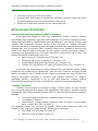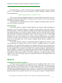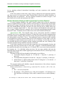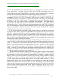
1
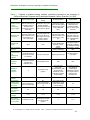
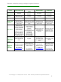
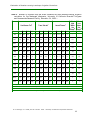
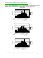
University of California Cooperative Extension Center for Landscape and Urban Horticulture EVALUATION OF WEATHER-SENSING LANDSCAPE IRRIGATION CONTROLLERS January through December 2003 A Report Submitted to: Office of Water Use Efficiency California Department of Water Resources June 2004 Dennis R. Pittenger Area Environmental Horticulture Advisor University of California Cooperative Extension Los Angeles County / Dept. of Botany & Plant Sciences University of California Riverside David A. Shaw Landscape and Turfgrass Advisor University of California Cooperative Extension San Diego County William E. Richie Staff Research Associate University of California Cooperative Extension Dept. of Botany & Plant Sciences University of California Riverside Copyright © 2004. Regents of the University of California For copies of this report or additional information concerning the study, please contact: Dennis Pittenger U. C. Cooperative Extension Batchelor Hall Extension U.C. Riverside Riverside, CA 92521 Telephone: 951.827.3320 Email: [email protected] The University of California prohibits discrimination or harassment of any person on the basis of race, color, national origin, religion, sex, gender identity, pregnancy (including childbirth, and medical conditions related to pregnancy or childbirth), physical or mental disability, medical condition (cancer-related or genetic characteristics), ancestry, marital status, age, sexual orientation, citizenship, or status as a covered veteran (covered veterans are special disabled veterans, recently separated veterans, Vietnam era veterans, or any other veterans who served on active duty during a war or in a campaign or expedition for which a campaign badge has been authorized) in any of its programs or activities. University policy is intended to be consistent with the provisions of applicable State and Federal laws. Inquiries regarding the University’s nondiscrimination policies may be directed to the Affirmative Action/Staff Personnel Services Director, University of California, Agriculture and Natural Resources, 300 Lakeside Drive, 6th Floor, Oakland, CA 94612-3550, (510) 987-0096. Evaluation of Weather-sensing Landscape Irrigation Controllers Table of Contents EXECUTIVE SUMMARY........…………………………………………………………………. i INTRODUCTION.....……………………………………………………………………………. 1 BACKGROUND AND OBJECTIVES......................…………………………………………… 1 METHODS AND PROCEDURES.......………………………………………………………..... 4 Selection and Initial Assessment of SWAT Controllers………………………………… 4 Irrigation Treatments……………………………………………………………………. 4 Reference Irrigation System and Treatment Calculations………………………………. 5 Data Collection…………………………………………………………………………...6 RESULTS………………………………………………………………………………………... 6 Assessment of Interface and Setup……………………………………………………… 6 Weather Parameters Employed and Programming Procedures Required………………. 7 Evaluation of Irrigation Schedules…………………………………………………...... 11 SUMMARY AND CONCLUSIONS…………………………………………………………... 14 TABLES Table 1: Features of weather-sensing irrigation controllers evaluated..................…….. 16 Table 2: Number of irrigation days per week scheduled by three weather-sensing irrigation controllers for five landscape treatments………………………… 18 FIGURES Figure 1: Weather sensing irrigation controllers evaluated…….………………………. 19 Figure 2: Irrigation applied by an Aqua Conserve controller compared to ETo and UCR references for 3 landscape treatments.………………………........ 20 Figure 3: Irrigation applied by a WeatherSet controller compared to ETo and UCR references for 3 landscape treatments.………………………………… 21 Figure 4: Irrigation applied by a WeatherTRAK controller compared to ETo and UCR references for 3 landscape treatments.………………………………… 22 Figure 5: Irrigation applied by a WeatherTRAK controller at mixed high and mixed low water use plants settings compared to ETo…………………………... 23 LITERATURE CITED…………………………………………………………………………. 24 D. R. Pittenger, D. A. Shaw, and W. E. Richie. 2004. University of California Cooperative Extension. Evaluation of Weather-sensing Landscape Irrigation Controllers EXECUTIVE SUMMARY Irrigation controllers that set and adjust water application in response to changes in the weather are now available for residential and commercial use. These devices are commonly termed “weather-sensing", “ET”, or “weather-based” irrigation controllers, and the technology is collectively referred to by the irrigation industry as Smart Water Application Technology, or SWAT. Many of the dozen or so devices now available automate the use of reference evapotranspiration (ETo) data or other environmental parameters correlated with evapotranspiration (ET) and plant water demand. Ideally, SWAT products take irrigation management out of peoples’ hands by automatically scheduling landscape irrigation. Their use theoretically can simplify and improve landscape irrigation scheduling, minimize runoff, and result in measurable water conservation. Although there have been several studies on the performance of various SWAT devices, few of them provide scientific and objective analysis of a product’s or technology’s performance. None of the studies referenced water used (or water saved) objectively to plant performance, so it is difficult to judge if the amount of water applied was over, under, or equal to the plants’ real-time needs for acceptable landscape performance, optimum growth, or other plant-based criteria. In 2003, we conducted a science-based evaluation of selected weather-sensing irrigation controllers to determine the climatic data the controllers use, how easy they are to setup and operate, and how closely their irrigation regimes match landscape irrigation needs established by previous field research. The products and models included in the study were Aqua Conserve ET6 (Aquaconserve, Riverside, CA), WeatherSet WS16 (The WeatherSet Co., Winnetka, CA), WeatherTRAK (Hydropoint Data Systems, Inc., Petaluma, CA), and Calsense ET1 with an electronic ET gauge (California Sensor Corp., Carlsbad, CA). The programming procedures followed with each controller, the weather parameter(s) they employed, and the ease of interface and setup for each product were documented and appraised. Stations on each controller were set up and programmed according to the manufacturer’s directions to schedule irrigation automatically from January through December 2003 for the following hypothetical landscape plantings: Cool-season turfgrass (tall fescue) at optimum quality (Treatment 1) Trees/shrubs (Treatment 2). Annual flowers, or about 100% ETo (Treatment 3). Two additional stations were set up on the Weather TRAK product during the winter and summer of 2003, respectively, using the unit’s following pre-set programs: Mixed high water use plants (Treatment 4). Mixed low water use plants (Treatment 5). The SWAT devices virtually controlled an existing reference irrigation system and used its system performance data as required in their initial setup. Simultaneously, the reference irrigation system was used to apply the correct amount of water to a real-time tall fescue turfgrass planting whose water needs served as the reference standard treatment comparison for the cool-season turfgrass treatment. Reference standard treatments for trees/shrubs and annual D. R. Pittenger, D. A. Shaw, and W. E. Richie. 2004. University of California Cooperative Extension. i Evaluation of Weather-sensing Landscape Irrigation Controllers flowers treatments were calculated using on-site, real-time ETo data and plant factors developed primarily from previous research. The weekly amount of irrigation actually applied to the reference turfgrass planting was recorded as were the weekly amounts of calculated irrigation required by the other reference treatment plantings. The station runtimes of the controllers evaluated were recorded and converted to depth of applied water using the performance characteristics of the reference irrigation system the controllers virtually operated. The weekly cumulative depths of water applied by controllers were summarized into monthly totals and compared to the real-time cool-season grass reference applications and the calculated reference standard amounts for the other treatments. The results of this study show each controller evaluated adjusted its irrigation schedules through the year roughly in concert with weather and ETo changes, but the magnitudes of their adjustments were not consistently in proportion to the changes in real-time ETo. Unfortunately, no product was able to produce highly accurate irrigation schedules consistently for every landscape setting when compared to research-based reference comparison treatments. Aqua Conserve was the simplest, easiest to operate, and most appropriate for homeowner use of those products studied. It applied water at the correct frequency and irrigated trees/shrubs with reasonably good precision, but it tended to apply more water than needed to all landscape treatments, especially in the summer for cool-season turfgrass. Calsense ET1 with an electronic ET gauge input offered the most complex interface, and it was equally as complex to set up. Since the electrical connections and function of the electronic ET gauge repeatedly failed in our study, it was impossible to evaluate fairly its weather-based irrigation scheduling capabilities. WeatherSet was simple and easy to use but visually intimidating. It produced very inaccurate irrigation schedules that would have damaged plants due to severe under-irrigation. WeatherTRAK was the most sophisticated controller studied and the most flexible in addressing the specific parameters found in each landscape setting, but it requires a professional landscape manager (or equivalently trained individual) to setup the unit accurately. It provided relatively accurate irrigation schedules for cool-season grass, but grossly over-watered the trees/shrubs treatment. Other important findings and conclusions from the controllers studied are: greater complexity and technicality of required setup information does not necessarily result in more accurate, water-conserving irrigation schedules. adoption of SWAT will not eliminate human interaction in landscape irrigation management. weather-sensing controllers will likely require professional monitoring and follow-up adjustment of their initial irrigation schedules. use of weather-sensing controllers does not assure landscape water conservation or acceptable landscape plant performance. D. R. Pittenger, D. A. Shaw, and W. E. Richie. 2004. University of California Cooperative Extension. ii Evaluation of Weather-sensing Landscape Irrigation Controllers INTRODUCTION Advances in irrigation control technology provide numerous tools to landscape managers, homeowners, and water agencies for conserving water in urban landscapes. Irrigation controllers that set and adjust water application in response to changes in the weather are now available for residential and commercial use. Many of these devices utilize reference evapotranspiration (ETo) data to calculate landscape water budgets and determine irrigation schedules. Historical and real-time ETo data are widely available in California, and while any automatic irrigation controller can be set to apply ETo-based schedules, the calculations and programming involved are laborious and too complicated for many people to implement. An alternative method is to install an irrigation controller that automatically adjusts watering schedules based on local weather data, or other environmental parameter correlated with ETo and plant water demand. In 2003, we conducted a science-based evaluation of selected weather-sensing irrigation controllers at the University of California Riverside Turfgrass and Ornamentals Research Facility. The study was designed to determine the climatic data the controllers use, how easy they are to setup and operate, and how closely their irrigation regimes match landscape irrigation needs established by previous field research. This report provides the results of the study and our conclusions. BACKGROUND AND OBJECTIVES There are at least 12 irrigation control products that automatically schedule irrigation based on local weather or other environmental parameters (California Urban Water Conservation Council, 2003). These devices are commonly termed “weather-sensing", “ET”, or “weatherbased” irrigation controllers, and the technology is collectively referred to by the irrigation industry as Smart Water Application Technology, or SWAT. The devices replace a traditional controller, or work in coordination with a traditional controller, and have proprietary hardware and/or software that automatically receive(s) or access(es) real-time or historical ETo information or other type of environmental data to schedule and adjust landscape irrigation according to the local weather. The technologies and user interfaces employed by SWAT devices vary in complexity from traditional controller features and layouts to Internet-based management and interface. Some rely on remote communication to a data source via a telephone line, paging signal or similar technology while others use historical ETo data modified by on-site temperature, solar radiation, or other environmental input sensors. Weather-sensing controllers are intended to efficiently irrigate landscapes by automatically calculating and implementing irrigation schedules that apply the right amount of water at the right time. Centralized irrigation control using a computer, on-site weather station data, and sophisticated valve control has been widely adopted by golf courses and other large irrigated facilities. These systems rely on advanced technology and are closely attended to by welltrained qualified personnel. In contrast, the SWAT controllers are intended to be less technical in nature and include residential and small commercial landscapes in their target audience. For residential and commercial landscapes, the SWAT controllers eliminate hand calculation of ETobased irrigation schedules for each irrigation station, and ideally, they can take irrigation D. R. Pittenger, D. A. Shaw, and W. E. Richie. 2004. University of California Cooperative Extension. 1 Evaluation of Weather-sensing Landscape Irrigation Controllers management out of peoples’ hands by automatically scheduling landscape irrigation. Their proprietary algorithms purportedly tailor the amount and timing of water applied to meet the specific real-time needs of the plants and, in some cases, address the constraints of a site such as cycling irrigation of slopes to reduce runoff. In theory, the use of these devices in residential and commercial landscapes will simplify and improve landscape irrigation scheduling, minimize runoff, and result in measurable water conservation. SWAT products vary in price from about $100 to over $3,000 depending on the number of stations controlled and other variables, and some require a set-up fee or an on-going service fee in the range of $25/yr to $250/yr (California Urban Water Conservation Council, 2003). Services of a professional landscape manager may be required to perform the initial setup of the controller and irrigation stations depending on the complexity and technical knowledge required by a device. There have been several studies regarding the reliability and water conservation achieved with SWAT. A study was conducted in Boulder, CO with granular matrix sensors (GMS or WatermarkTM) placed in the soil to interrupt pre-set irrigation schedules of standard irrigation control valves whenever soil moisture was adequate for turfgrass needs (Qualls et al., 2001). The system was field calibrated so that the GMS would prohibit valve operation until soil moisture content dropped to a point where turfgrass showed signs of stress. Comparing actual applied water controlled by the GMS to calculated potential ET using a temperature-modified Blaney-Criddle method (B-CT), the investigators documented that GMS-controlled irrigation was 70% of the B-CT modified ET. The amount of water applied was roughly equivalent to the minimum water requirement of cool-season grass grown in Irvine, California as reported by Meyer and Gibeault, 1986 and Gibeault et al., 1990, which is less than that required for optimum cool-season grass performance. Studies were conducted during 2001 in Denver and two water districts in Northern California to document residential irrigation applied by Aqua Conserve ET controllers (Addink and Rodda, 2002). In Denver, the water used by 37 participating landscapes (17 equipped with real-time temperature sensors) was compared to their 5-year historical usage and over 800 nonparticipating residential irrigation users. In Northern California, Aqua Conserve controllers (all equipped with real-time temperature sensors) were installed at 37 residential sites identified by the water agencies as “high volume users”. Their water usage in 2001 was compared to their 2or 5-year historic average use. Results showed substantial variation with some participants having extremely high water savings, some no water savings, and a few with increased water usage. Overall, the investigators concluded that residential landscape irrigation was reduced 7% to 25% by using this product, and water districts will realize a significant reduction in total water demand, although limited data was presented to support this. Similarly, preliminary results from an on-going pilot program at 29 sites in Los Angeles, both residential and commercial, involving two SWAT controller products (WeatherTRAK and Water2Save) was showing irrigation “savings” as follows: 14% are saving 2% to 10%, 38 % are saving 10% to 30%, 24% are saving 33% to 79%, and 24% are increasing water use 8% to 71% (Estrada, 2003). The findings are for the latter half of 2002 and early 2003, representing a period where plants’ water demand decreases dramatically from mid-summer into winter, a period when irrigation managers often neglect to re-program controllers accordingly. However, the basis for establishing water savings in this project was not provided. D. R. Pittenger, D. A. Shaw, and W. E. Richie. 2004. University of California Cooperative Extension. 2 Evaluation of Weather-sensing Landscape Irrigation Controllers A single-season study in Colorado among 10 participants interested in conserving landscape water, showed the WeatherTRAK product irrigated landscapes at about 81% of ETo which reduced landscape irrigation about 20% from the amount sites historically used after accounting for real-time variance (Aquacraft, 2002). However, when SWAT controllers were installed, participants were made aware of irrigation system problems (i.e. dysfunctional sprinkler heads and poor system uniformity) and asked to remedy them, but there was no assessment of the impact of improvements’ on irrigation system performance or on changes in irrigation requirements. Based on the data provided in the report, applied water plus rainfall would have been enough for optimal cool-season grass ET, but there was no plant-based evaluation of the controller’s performance. The results indicate that many of the participants were significantly over-irrigating their landscapes prior to installing this product. Most of the participants liked the system but were unwilling to pay its on-going $49/yr service fee. Other widely reported studies of WeatherTRAK’s residential landscape performance in Irvine, California (Hunt et al., 2001 and Bamezai, 2001) state this product applied water very close to the ET-based water budget for the participating households without sacrificing plant performance, but objective plant performance evaluations were not employed. A 2002 study in Seattle (Seattle Public Utilities, 2003) found the use of the Aqua Conserve controller with a rain sensor significantly reduced applied water when weather factors were accounted for. Participants were mostly satisfied with the product, and 85% expressed their landscape’s quality was as good as or better than before the product was installed. A small number of these prior studies provide any scientific and objective analysis of a product’s or technology’s performance. Most were observational studies or demonstrations in which a controller manufacturer conducted the study or their representative was integrally involved in conducting the study. Projects were typically designed so that it was difficult or impossible to know how much change in water use was the result of the controller’s performance versus the weather or other factors. The studies usually compared historical water use with water use after a weather-based controller product was installed without normalizing results to account for differences between real-time and historical weather conditions or without accurately determining how efficiently the landscapes were irrigated prior to utilizing the new controller. Few studies referenced applied water to ETo. None of the studies referenced water applied (or water saved) objectively to plant performance, so it is difficult to judge if the amount of water applied was over, under, or equal to the plants’ real-time needs for acceptable landscape performance, optimum growth, or other plant-based criteria. Since studies did not objectively and scientifically evaluate how plant material performed in response to the amount of water applied by the weather-sensing controller, they lack an objective basis for measuring changes in water use. Urban water agencies, landscape and turfgrass management professionals, and homeowners, are interested in adopting weather-sensing irrigation controllers, but, because of the limitations of previous studies and reports, they are unsure about the effectiveness of these devices in conserving water while meeting landscape irrigation needs. The objectives of this study were to evaluate selected weather-sensing irrigation controllers and: 1. Discern the type of climatic or weather data the devices use to calculate irrigation schedules automatically. D. R. Pittenger, D. A. Shaw, and W. E. Richie. 2004. University of California Cooperative Extension. 3 Evaluation of Weather-sensing Landscape Irrigation Controllers 2. Assess the complexity of their setup and use. 3. Determine their effectiveness in automatically scheduling irrigation regimes that match ETo-based landscape water needs established by field research. 4. Identify and evaluate their potential as water conservation tools. METHODS AND PROCEDURES Selection and Initial Assessment of SWAT Controllers In the spring and summer of 2002, four commercially available controller products, representing unique proprietary approaches and technologies for providing automated weathersensing irrigation control in residential and commercial landscapes, were selected for study at the Turfgrass and Ornamentals Research Facility at the University of California Riverside. Selections were based on discussions with water agency personnel and controller manufacturers. Although there were several other SWAT irrigation control devices available or arriving in the market at the time the study was initiated, the four products selected represented a range of technologies and approaches in use (California Urban Water Conservation Council, 2003). The products and models included in the study were: Aqua Conserve ET-6 (Aquaconserve, Riverside, CA). WeatherSet WS16 (The WeatherSet Co., Winnetka, CA). WeatherTRAK (Hydropoint Data Systems, Inc., Petaluma, CA). Calsense ET1 with electronic ET gauges (California Sensor Corp., Carlsbad, CA). At the outset, the programming procedures followed with each controller and the weather parameter(s) they employed were documented. Also, the ease of interface and setup for each product was judged as “easy” (friendly interface; simple to understand and set up with little or no technical horticultural knowledge or experience with irrigation controllers) or “complex” (unfriendly interface; complicated to set up with input parameters requiring technical horticultural knowledge and experience with landscape irrigation control and management). Irrigation Treatments Controllers did not irrigate real landscape settings. Instead, stations on each controller were set up and programmed according to the manufacturer’s directions to schedule irrigation automatically from January through December 2003 for the following hypothetical landscape plantings: Cool-season turfgrass (tall fescue) at optimum quality (Treatment 1) Trees/shrubs (Treatment 2). Annual flowers, or other planting requiring the upper few inches of soil to remain moist, or about 100% ETo (Treatment 3). Two additional stations were set up on the Weather TRAK product during the winter and summer of 2003, respectively, using the unit’s following pre-set programs: Mixed high water use plants (Treatment 4). Mixed low water use plants (Treatment 5). D. R. Pittenger, D. A. Shaw, and W. E. Richie. 2004. University of California Cooperative Extension. 4 Evaluation of Weather-sensing Landscape Irrigation Controllers Only the minimum information required for a controller to schedule irrigation automatically for the landscape settings was provided in the initial setup. No additional information was entered and no manual adjustments were enacted to modify controllers’ programs or station runtimes so an evaluation could be made of each unit’s built-in “knowledge” and ability to apply automatically the “correct” amount of irrigation. Controllers were not manually shut off during rain events. For the WeatherTRAK product, which can utilize additional site and system parameter data to calculate custom schedules, the details for system performance data, soil texture, and root depth were input for the cool-season grass station in midAugust to determine if greater irrigation precision resulted by entering this information. Reference Irrigation System and Treatment Calculations The SWAT devices virtually controlled an existing reference irrigation system and used its system performance data as required in their initial setup. This reference system was operated by an independent controller and had a precipitation rate (PR) of 0.93 in/hr (23.6 mm/hr) and a low quarter distribution uniformity (DU) of 0.81. The reference irrigation system was used to apply the correct amount of water to a real-time turfgrass planting for this study and other landscape research plots at the Turfgrass and Ornamentals Research Facility of the University of California Riverside. Standards for programming the reference irrigation system and determining how closely a controller’s irrigation schedules met the needs of cool-season turfgrass and trees/shrubs were established based on previous field research findings, while the reference for annual flowers (or plantings requiring the soil surface to remain moist) was set at 100% ETo. Weekly ETo and rainfall data were collected from CIMIS (California Irrigation Management Information System) station #44 at U.C. Riverside, located approximately 165 ft (50 m) from the irrigated plots. Crop coefficient (Kc) values and plant factors were used with the ETo data to calculate the irrigation requirements of the reference plantings. For cool-season turfgrass, the reference standard treatment (UCR 1) was an actual planting of tall fescue located at the research facility irrigated by the reference irrigation system to maintain optimum turf quality (Gibeault et al., 1990; Pittenger et al., 2002). Its irrigation was scheduled 3 days each week (Tuesday, Thursday, and Saturday) with up to 6 cycles per day by the equation: Weekly irrigation amount = [(ETo X Kc) – R] / DU, where: ETo is the previous week’s cumulative ETo from CIMIS; Kc is the monthly cool-season turfgrass Kc (Gibeault et al., 1990); R is rainfall >0.1 in (2.5 mm); DU is the distribution uniformity of the irrigation system. The reference standard treatment for the trees/shrubs station’s irrigation schedule (UCR 2) was one irrigation day per week (Wednesday) with the amount based on findings of Pittenger et al., 2002 and Shaw and Pittenger, 2004. The irrigation amount was calculated as Weekly irrigation amount = weekly ETo x 0.50. D. R. Pittenger, D. A. Shaw, and W. E. Richie. 2004. University of California Cooperative Extension. 5 Evaluation of Weather-sensing Landscape Irrigation Controllers The annual flowers (or other water-stress sensitive planting) irrigation reference standard (UCR 3) was scheduled 4 days per week (Sunday, Tuesday, Thursday, Saturday) with the amount calculated as Weekly irrigation amount = weekly ETo / DU. There were no reference standards available for the mixed high and mixed low water use treatments scheduled by WeatherTRAK (Treatments 4 and 5) because it was not clear what plant materials these programs represent. Irrigation days were eliminated in the reference standards fall through spring when ETo was low or rainfall was significant. Data Collection The weekly amount of irrigation actually applied to the reference turfgrass planting was recorded as were the weekly amounts of irrigation virtually applied to the other reference treatment plantings. While the controllers evaluated did not irrigate actual landscape plantings, their station run times were recorded in tenths of minutes by electro-mechanical time counters (IVO model B148.001; Genesis Automation, Powell, OH) wired to receive the electrical signal generated when a controller powered the circuit to open an irrigation valve. The weekly cumulative run times were recorded for all stations by the counters and the days irrigation occurred were noted. Run time minutes were converted to depth (millimeters) of applied water based on the precipitation rate of the reference irrigation system that the controllers were virtually operating. The weekly cumulative runtimes, corresponding depths of applied water, and ETo values were summarized into monthly totals in order to provide a meaningful analysis of controller performance. The virtual amounts applied by the controllers studied were then compared to the amounts actually applied to the cool-season grass reference plot and the amounts calculated to have been applied to the trees/shrubs and annual flower reference plantings. Monthly amounts of water applied by a controller were compared to the calculated reference standard amounts and judged equal to the reference amount when applied water was ±10% of the reference, slightly over/under the reference when within ±11% to 20%, moderately over/under the reference when within ±21% to 40% of the target, and well over/under the reference when applied water was >40% (±) of the target. RESULTS Assessment of Interface and Setup The Aqua Conserve controller was judged to have the friendliest interface and to be the easiest to set up. The WeatherSet device followed it closely. WeatherSet was easy to use once setup commenced, but its interface panel was visually intimidating at first. The WeatherTRAK offered an easy and friendly interface but was complex to set up because it required a great deal of technical horticultural information to achieve precision. Calsense’s ET1 with an electronic ET gauge presented the most complex interface, and it was equally as complex as WeatherTRAK to D. R. Pittenger, D. A. Shaw, and W. E. Richie. 2004. University of California Cooperative Extension. 6 Evaluation of Weather-sensing Landscape Irrigation Controllers set up, requiring technical horticultural knowledge and some experience with controller programming. Of the four products in this study, Aqua Conserve offered the most appropriate interface and setup process for homeowners, while WeatherTRAK offered the greatest flexibility in addressing unique site parameters. The four irrigation controllers are shown in Figure 1, and their features are reviewed and summarized in Table 1. Weather Parameters Employed and Programming Procedures Required To derive irrigation schedules, the Aqua Conserve product used an on-site temperature sensor to modulate historic ETo data, Calsense used real-time ETo estimated from an electronic atmometer (ET gauge), WeatherSet used an on-site solar radiation sensor to adjust historic ETo data, and WeatherTRAK used daily real-time ETo data from the on-site CIMIS station #44, received via a paging signal (Table 1). The Aqua Conserve and WeatherSet units require the user to input a location which the controller uses for selecting and adjusting internally stored historical ET data. WeatherSet also used data from a rain sensor included with the unit. Aqua Conserve ET6: This controller looks, sets up, and operates much like a standard controller, but it uses a combination of historic ETo data and on-site, real-time temperature data to modulate stations’ runtimes daily from their average July peak schedule that is supplied by the user during initial set up (Table 1, Fig. 1). The temperature sensor is connected to the controller via an insulated wire and is mounted within 50 feet of the irrigated site on the south or west side of a building in a shaded location such as under an eave or overhang. For the study, the sensor was mounted adjacent to the irrigated reference turfgrass plot under the west overhang of the irrigation equipment shed in which the controller was housed. To set up the controller, the user enters the current time, date and geographic location, and then assigns water days and start times to each of the 3 programs. From the information input, the controller then places the unit along one of 16 historic ETo curves most closely matched to the irrigation site. For individual station run times, the user must calculate and enter the maximum daily run time that would be applied given each station’s PR, DU, and run days in July (the highest ET month). The initial average July base schedules for this study were as follows: Cool-season turfgrass (Program A): 135 min/wk = 3 days/wk, 3 cycles/day, 15 min/cycle. Trees and shrubs (Program B): 58 min/wk = 1 day/wk, 3 cycles/day, 19 min/cycle. Annual flowers or plants needing about 100% ET (Program C): 116 min/wk = 4 days/week, 3 cycles/day, 10 min/cycle. The program runtimes and schedules, using the characteristics of the reference irrigation system, were calculated as follows: Weekly runtime minutes = (historical avg. weekly July ETo × July Kc) ÷ (DU × PR) × 60, where, ETo = 1.8 in/wk (45 mm/wk). Kc turfgrass = 0.94 (Gibeault et al., 1990), Kc trees/shrubs = 0.5 (Pittenger et al., 2002 and Shaw and Pittenger, 2004), and Kc annual flowers or similar planting = 1.0. D. R. Pittenger, D. A. Shaw, and W. E. Richie. 2004. University of California Cooperative Extension. 7 Evaluation of Weather-sensing Landscape Irrigation Controllers DU = 0.81, the distribution uniformity of the irrigation system, which was used only in the turfgrass schedule calculations. PR = 0.93 in/hr (2.55 min/mm), the precipitation rate of the irrigation system. 60 = the factor required to convert units to minutes. Using the equation and values above produced the average July base Weekly Runtime Minutes: Cool-season grass = (1.8 in. × 0.94) ÷ (0.81 × 0.93 in/hr) × 60 = 135 min. Trees/shrubs = (1.8 in. × 0.5) ÷ (0.93 in/hr) × 60 = 58 min. Annual flowers/similar planting = (1.8 in. × 1.0) ÷ (0.93 in/hr) × 60 = 116 min. The total minutes were then divided by the weekly number of run days and cycles per day. Final program run times for the three landscape scenarios were 15 minutes for turfgrass, 19 minutes for trees/shrubs, and 10 minutes for annual flowers for each run time within a cycle and day. Although the Aqua Conserve controller display continues to show the initial run times, the actual run times are automatically adjusted (usually downward) from the initial average July runtime setting according to the historical ETo curve and the temperature sensor input. There is an “Accumulation” feature option that eliminates extremely short watering runtimes in cool weather. With the Accumulation feature on, the controller will skip days until at least 50% of the water time has accumulated and then water on the next scheduled day. With the Accumulation feature off, the controller will water on the program days. The controller also offers a “Water Reduction” feature that globally reduces the watering times for all programs by an entered percentage. To see a log of total run time for the past 7 days, one pushes and holds the “previous” button with the dial on “Run”. The display toggles through the run time for each of the six stations. When the “Next” button is held down, the display toggles through the current day’s run time for each station. Directions for parameters that can be viewed when the dial is on “Run” are displayed on the front panel of the controller and are easy to understand. Calsense ET1 with electronic ET gauge input: Initial setup of the Calsense ET1 includes entering time, date, etc. much like a standard controller. It uses the ET gauge to obtain on-site, real-time ETo data that is then used with optional programmed Kc values and user-supplied data about the irrigation system to adjust irrigation amounts for each station (Table 1, Figure 1). The ET gauge is connected to the controller and mounted on a nearby post which has turfgrass fetch around it, but in a location which gets minimum sprinkler precipitation (irrigation water tends to seal up the felt and ceramic surface of the atmometer). When used with an atmometer, the controller is set up with “real-time ET from ET gauge”. The ET gauge was powered with AA batteries in this study, although it can be powered directly by the controller power supply. Programs are defined with water days and start times first and then stations are assigned to programs as desired. Start times can be assigned to each program so they do not overlap. Setup requires a precipitation rate for each station so it can calculate time and depth of water application. After completing setup, a percentage of ET can be manually entered for each station to account for uniformity losses or other parameters and factors unique to the station. D. R. Pittenger, D. A. Shaw, and W. E. Richie. 2004. University of California Cooperative Extension. 8 Evaluation of Weather-sensing Landscape Irrigation Controllers Unfortunately, in the Calsense system, the electrical connections and function of the electronic ET gauge repeatedly failed making it impossible to keep it operating properly. This product was eliminated from the study in March, and none of its performance data is presented. WeatherSet: This controller has a unique user interface unlike a traditional controller. It utilizes an array of dials, toggles, dipswitches, and LED lights for user input and information feedback (Fig. 1). Data from a solar radiation sensor connected to the unit is used to adjust irrigation. The weekly irrigation schedule for each station is increased or decreased based on the cumulative solar radiation measured, termed “Sunfall” (Table 1). Proprietary algorithms calculate the Sunfall factor and use it with historical ETo to calculate irrigation schedules for stations based on set up information supplied by the user. For the study, the Sunfall sensor was sited adjacent to the irrigated turfgrass reference plots on the eve of the roof of the irrigation equipment shed where the controller was located. The sensor was not shaded at any time. To set up the WeatherSet controller, the user sets the current date and time, as well as a daily irrigation start time and a desired “no water” day for each valve. Similar to the Aqua Conserve unit, the user must calculate and set the maximum daily runtime required in the hottest weather for each valve station. For the study, the maximum daily runtime for each station was 19 min/day based on the average July schedule in the cool-season turfgrass research plots used for reference in the study. This daily runtime is equivalent to the maximum weekly runtime entered in the Aqua Conserve unit, which was the average weekly July time divided by 7 (135 min/wk ÷ 7 d/wk = 19 min). Next, the predominant plant material in the zone irrigated by each valve is selected as “lawn”, “groundcover/shrubs”, or “flowers”. With this information, the controller sets the irrigation days and runtimes automatically from algorithms that use the realtime solar radiation to calculate a Sunfall factor which adjusts historical ETo. The WeatherSet “groundcover/shrubs” program was used for the trees/shrubs treatment in the study. WeatherTRAK: The WeatherTRAK controller has the most distinctive appearance and user interface (Figure1), but it requires the most user input, both in volume and technical degree, of the four controllers evaluated (Table 1). Programming it for maximum precision in scheduling irrigation requires accurate knowledge of the landscape’s soil texture, microclimate, slope, plant type, plant rooting depth, and irrigation system. The controller has built-in information and algorithms that enable it to use local real-time ETo, received daily via wireless paging signal technology, with user-supplied site details to adjust irrigation schedules for each station in relation to weather conditions. Setup begins with the user setting a start time that is used for all stations. The current time, date, and zip code are also set. The manufacturer automatically assigns an ET Zone, maximum zone ET, and a water district code. The user scrolls via 2 dials through a list of selections and yes/no questions to set up each station. Fortunately, it comes with a detailed user’s manual that walks the operator through the setup and programming. For the study, setup was accomplished by enabling the Advanced Features. Each controller station was programmed for “fully automated” operation by following the setup steps for landscape scenarios of cool-season grass, trees/shrubs, annual flowers or other planting (needing about 100% ETo). The following procedure was used to program the WeatherTRAK D. R. Pittenger, D. A. Shaw, and W. E. Richie. 2004. University of California Cooperative Extension. 9 Evaluation of Weather-sensing Landscape Irrigation Controllers unit for the various treatments (inputs appear in parentheses and any parameters not listed were set to default values): Cool-season grass (Treatment 1): Set Station to Program (1) Set Program Mode (fully automated) Set Sprinkler type (mixed rotors) Set Plant Type (cool-season grass) Set Soil Type (sandy loam) Set Microclimate (sun all day) Set Slope Factor (none to slight, 0% slope) In mid-August, the following parameters were entered to obtain a custom schedule: PR = 0.93 in/hr and DU = 0.81. Tree/Shrub program (Treatment 2): Set Station to Program (2) Set Program Mode (fully automated) Set Sprinkler type (mixed rotors) Set Plant Type (trees) Set Soil Type (sandy loam) Set Microclimate (sun all day) Set Slope Factor (none to slight, 0% slope) Annual flowers or similar planting (Treatment 3): Set Station to Program (3) Set Program Mode (fully automated) Set Sprinkler type (mixed rotors) Set Plant Type (flowers) Set Soil Type (sandy loam) Set Microclimate (sun all day) Set Slope Factor (none to slight, 0% slope) Mixed High Water Use Plants (Treatment 4, set up Feb. 2003): Set Station to Program (4) Set Program Mode (fully automated) Set Sprinkler type (custom, PR = 0.93 in/hr and DU = 0.81) Set Plant Type (mixed high water use plants) Set Soil Type (sandy loam) Set Microclimate (sun all day) Set Slope Factor (none to slight, 0% slope) Set Root Depth (12 in) D. R. Pittenger, D. A. Shaw, and W. E. Richie. 2004. University of California Cooperative Extension. 10 Evaluation of Weather-sensing Landscape Irrigation Controllers Mixed Low Water Use Plants (Treatment 5, set up June 2003): Set Station to Program (5) Set Program Mode (fully automated) Set Sprinkler type (custom, PR = 0.93 in/hr and DU = 0.81) Set Plant Type (mixed high water use plants) Set Soil Type (sandy loam) Set Microclimate (sun all day) Set Slope Factor (none to slight, 0% slope) Set Root Depth (18 in) Evaluation of Irrigation Schedules Real-time reference ET (ETo) for 2003 was near historic ETo (Snyder, et al., 1987) in most months, but it was significantly less in July, implying that plant water use would have been somewhat less than average during that month (Figs. 2, 3, 4). Rainfall was only slightly less than normal for the 12-month period with significant rainfall in February and March (Figs. 2, 3, 4). Thus, the climate in 2003 was representative and provided a sound basis for testing the automated capabilities of the weather-sensing irrigation controllers. Actual applied irrigations to the cool-season turfgrass reference plots (UCR 1) provided the amount of water necessary for optimal turfgrass performance. The correct amount of water for trees/shrubs (UCR 2) and annual flowers (UCR 3) treatments were estimated mathematically. Each controller automatically adjusted irrigation of the three landscape settings in concert with changes in the seasons, weather conditions, and ETo, generally following a characteristic bell-shaped curve through the year (Figs. 2, 3, 4). The magnitudes of their adjustments were not consistently in proportion to the changes in real-time ETo, however. Frequency of irrigation (days/wk) that controllers watered each treatment is summarized in Table 2. Aqua Conserve. The estimated amount of irrigation applied to cool-season turfgrass by the Aqua Conserve unit was roughly equal to the amount required by the actual turfgrass reference planting (Aqua 1 vs. UCR 1) in March, April and May, but usually well over the reference planting in the other 9 months (Fig. 2). In the summer months, this controller applied irrigation to cool-season turfgrass exceeding ETo by 45% to 65%. Irrigation applied by Aqua Conserve to trees/shrubs was equivalent to or slightly over the reference amount calculated for this treatment (Aqua 2 vs. UCR 2) in January, February, March, May, and September (Fig. 2). However, applied water was well over the UCR 2 reference treatment in April, October, November, and December (Fig. 2). The amount of water applied to annual flowers or plantings needing about 100% ETo was typically moderately to well over the reference UCR 3 treatment irrigation amounts and well over ETo in the summer and fall (Fig. 2). The irrigation frequency determined by Aqua Conserve was consistently on par with the UCR reference for all landscape irrigation treatments (Table 2). It automatically eliminated water days in some weeks during the winter when ETo was very low so that runtimes did not become excessively short when the “Accumulation” feature was used. Because it lacked the optional rain sensor, Aqua Conserve sometimes scheduled irrigation in weeks when rainfall met D. R. Pittenger, D. A. Shaw, and W. E. Richie. 2004. University of California Cooperative Extension. 11 Evaluation of Weather-sensing Landscape Irrigation Controllers plants’ water needs. Adding a rain sensor would enable the Aqua Conserve to apply water at a highly accurate and effective interval in all seasons. Overall, Aqua Conserve delivered water at the correct frequency (Table 2) but tended to apply more water than needed to all landscape treatments (Fig. 2). Perhaps a follow up global adjustment in station runtimes using the “Percentage Reduction” feature would have enabled the unit to more accurately schedule irrigations. Aqua Conserve was most accurate in scheduling water to trees and shrubs where it closely met the water needs for acceptable performance of commonly grown trees/shrubs about ⅓ of the year. However, it typically applied more water than necessary for optimum cool-season turfgrass performance. For plantings needing about 100% ETo, it would ensure that these plant materials are well watered in the spring and summer, but it might over-water them in fall. It is likely that connecting a rain sensor to this product would greatly improve its irrigation scheduling, both frequency and amount, for turfgrass and annual flowers in rainy months, such as February and March of 2003. Weather Set. The estimated amount of water applied to cool-season turfgrass by the WeatherSet controller was equal to the actual turfgrass reference planting (WeatherSet 1 vs. UCR 1) in the winter (January, November, and December), but it was moderately to well under the reference for the remainder of the year (Fig. 3). Similarly, the trees/shrubs station typically applied only 20% to 30% of ETo in most months which was well under the calculated reference amount (Fig. 3). The amount of water applied to annual flowers or plantings needing about 100% ETo was relatively close to the reference in most months (Fig. 3), but it was moderately under the reference in the summer and part of the fall (June, July, August, and October), and well under it in the dry winter month of January. The frequency of irrigation determined by the WeatherSet unit was erratic for all the irrigation treatments (Table 2). In general, irrigations were scheduled more frequently in the summer months which were probably adequate for the cool-season turf and annual flowers (about 100 % ETo) treatments. However, for the trees/shrubs treatment, the increased frequency resulted in very short runtimes during the summer months. This practice usually results in shallow water penetration, and in combination with deficit irrigation it often results in poor landscape performance. The performance of the Weather Set unit indicates that with cool-season turfgrass there would have been brown or dead grass through most of the growing season. For trees/shrubs, extreme soil water deficits would have likely occurred during portions of the year. Many trees and shrubs might tolerate the wintertime water deficits produced by station WeatherSet 2, especially deciduous plants, but it is unlikely that many commonly grown species would perform acceptably with the extreme soil water deficits created in the summer. It is estimated that annual flowers and plantings needing 100% ETo would have been significantly under-watered in the summer but well-watered in the other seasons. WeatherTRAK. Irrigation water applied to cool-season grass by the WeatherTRAK unit was equal to the UCR 1 reference treatment in April and October but was slightly over or under the reference amounts during January, February, May, August, September, and December (Fig. 4). It moderately over-irrigated compared to UCR 1 in March, June, and July, and irrigated well over in November. There was no seasonal pattern to the deviation from the reference irrigation D. R. Pittenger, D. A. Shaw, and W. E. Richie. 2004. University of California Cooperative Extension. 12 Evaluation of Weather-sensing Landscape Irrigation Controllers amount. WeatherTRAK usually adjusted irrigation very appropriately in response to rainfall except in November. The input of specific values for DU and PR in mid-August to the coolseason turfgrass treatment (WeatherTRAK 1) appeared to improve WeatherTRAK’s scheduling precision, as seen in the reduced deviation from the reference treatment thereafter. In contrast, the estimated amounts of water applied to the trees/shrubs treatments were consistently well over the UCR 2 reference levels in every month of 2003 (Fig. 4). WeatherTRAK grossly over irrigated the trees/shrubs treatment in the summer and fall months, applying 2 to 3 times the UCR 2 amount. The applied water was at least 25% greater than ETo in February, June, July, August, October, November, and December. The annual flowers treatment was also moderately or well over-irrigated the in all months except January, March, April, and June (Fig. 4). Only in March were irrigation applications less than UCR 3, which may have been an appropriate response to rainfall during that month. However, the controller did not respond in this manner to rainfall in February. In all other months, WeatherTRAK 3 typically applied amounts of water well over real-time ETo. In the “mixed high water use plants” setting (WeatherTRAK 4), the amount of irrigation applied from April through August by WeatherTRAK was typically near ETo, but it was well under ETo in April and moderately over ETo in September and December (Fig. 5). Irrigation applied to “mixed low water use plants” (WeatherTRAK 5) from May through December was 40% to 50% of ETo except in May when it was 15% of ETo and in July when it was 60% of ETo (Fig. 5). Since no reference standards were available for these treatments, the accuracy and appropriateness of these schedules are unknown. The irrigation frequencies determined by the WeatherTRAK unit in the summer were 1 to 2 days/wk and 3 to 6 days/wk for the trees/shrubs and the annual flower treatments, respectively (Table 2). Irrigation was less frequent in the other seasons. The cool-season turfgrass setting, however, was irrigated much more frequently than the UCR 1 reference in the spring and summer. The irrigation frequencies for trees/shrubs and annual flowers were horticulturally sound. Conversely, the near daily spring and summer irrigation frequencies for turfgrass were considered unsound because they often result in shallow water penetration and, if water amounts are sufficient, may increase disease and weed problems. WeatherTRAK’s performance indicates that cool-season grass would have been irrigated very effectively ¾ of the year but significantly over-irrigated for the remainder. Unfortunately, the unit tended to over-irrigate in the summer months when ET was highest. Adding custom PR and DU values in the set up parameters improves the precision of the controller’s irrigation scheduling. Nevertheless, commonly used trees and shrubs would be significantly over-irrigated to such a degree that excess growth and/or reduced root health would be expected. Newly planted annual flowers or a new lawn would be well irrigated in the winter and spring but probably over irrigated in the summer and fall. Use of the “mixed high water use plants” default setting would be expected to provide irrigation approximating 100% ETo, while the “mixed low water use plants” default setting would usually provide irrigation of 40% to 50% of ETo. However, the irrigation schedules for these two settings deviated significantly from these values during a few months. D. R. Pittenger, D. A. Shaw, and W. E. Richie. 2004. University of California Cooperative Extension. 13 Evaluation of Weather-sensing Landscape Irrigation Controllers SUMMARY AND CONCLUSIONS The results of this study provide useful information and a science-based perspective about the performance and potential benefits of weather-based irrigation control technology. Each controller studied adjusted its irrigation schedules through the year roughly in concert with weather and ETo changes, so that irrigation was automatically and substantially reduced in fallwinter-spring versus summer. However, the magnitudes of their adjustments were not consistently in proportion to the changes in real-time ETo. It was also clear that incorporation of a rain sensor or other accurate means of accounting for local rainfall is essential for a weathersensing controller to calculate correct irrigation schedules. Unfortunately, no product was able to produce highly accurate irrigation schedules consistently for every landscape setting when compared to research-based reference comparison treatments. The findings suggest that weather-sensing irrigation controller manufacturers need to reassess their algorithms and formulae used by the controllers in order for them to provide more precise irrigation schedules. Further study is needed to determine if the shortcomings of the units evaluated are related to self-contained ETo data, assumed Kc values, proprietary “adjustment factors” used, the weather-sensing method employed, or the weather sensing instrument used by the unit. Regrettably, problems with the ET gauge prohibited us from fully evaluating the Calsense controller. Furthermore, the findings indicate that adoption of SWAT will not eliminate human interaction in landscape irrigation management. Some products require users to calculate a base schedule in the setup process, while others require detailed technical knowledge in horticulture and irrigation management to set them up. Each controller evaluated would have required significant manual adjustment of its schedules to irrigate the landscape treatments accurately. The inability to provide accurate irrigation schedules without significant ‘tweaking’ indicates that weather-sensing or SWAT controllers will usually require professional monitoring and follow-up adjustment to their input parameters and/or manual modification of their schedules for a considerable period after the initial setup in order to realize the optimum irrigation program for each station. Users should first look to reduce runtimes and/or frequency because schedules tend to exceed plants’ needs according to our findings. Evaluation of plant response, expectations of the landscape’s appearance, and other factors will need to guide the necessary adjustments. It is important to note that many SWAT manufacturers, including those represented in this study, continue to adjust and/or re-design the algorithms and features of their products to improve their capabilities. Perhaps the most important factor affecting weather-based irrigation controller performance is the quality and accuracy of the information supplied when setting it up. For example, Aqua Conserve’s relatively easy to setup and ability to deliver accurate schedules is heavily reliant on the user knowing and entering a July base schedule that is accurate for the plants irrigated, while WeatherTRAK’s relatively complex setup information requires the user to have a relatively good technical understanding of the site and the plants irrigated. However, greater complexity and technicality of required setup information does not necessarily result in more accurate, water-conserving irrigation schedules, as was demonstrated in the trees/shrubs schedule calculated by WeatherTRAK (complex and technical setup) versus that of Aqua Conserve (simple, non-technical setup). D. R. Pittenger, D. A. Shaw, and W. E. Richie. 2004. University of California Cooperative Extension. 14 Evaluation of Weather-sensing Landscape Irrigation Controllers Each product studied demonstrated significant strengths and weaknesses summarized below. Aqua Conserve was the simplest, easiest to operate, and most appropriate for homeowner use of those products studied. When the user-supplied base setup schedule is accurate, as it was in the study, it applied water at the correct frequency but tended to apply more water than needed to all landscape treatments. It irrigated trees/shrubs with reasonably good precision, however. Possibly Aqua Conserve employs a factor for non-uniformity of irrigation systems in its algorithm(s) that results in over-irrigation if uniformity is already factored into a station’s base setup schedule, as was notable in this study with cool-season turfgrass and annul flower treatments. Calsense ET1 with an electronic ET gauge input offered the most complex interface, and it was equally as complex to set up. Since the electrical connections and function of the electronic ET gauge repeatedly failed in our study it was impossible to evaluate fairly its weather-based irrigation scheduling capabilities. WeatherSet was simple and easy to use but visually intimidating. It produced very inaccurate irrigation schedules that would have damaged plants due to severe under-irrigation. These results suggest that the product had not been effectively field tested prior to the study. However, WeatherSet incorporates a theoretically and scientifically sound approach for modulating historical ETo using a measure of solar radiation, which is the principal driver of plant water use. Refinement of the algorithms or the solar energy units employed might result in improved reliability and accuracy of irrigation schedules. Hopefully, the newer models released by WeatherSet will overcome these deficiencies. WeatherTRAK was the most sophisticated controller studied and required the most technical knowledge on the part of the user. It is very flexible in addressing the specific parameters found in each landscape setting, but it requires a professional landscape manager (or equivalently trained individual) to setup the unit accurately. In this study, WeatherTRAK provided relatively accurate irrigation schedules for cool-season grass, but tended to over-irrigate other plantings, grossly over-watering trees/shrubs treatments. The results of this study demonstrate that use of a weather-sensing controller does not assure landscape water conservation. Conservation can occur only if previous water use was known to be excessive and the schedules produced by the weather-sensing controller match the water needs of turfgrass and landscape plant materials. If previous water use was on target for the plant material’s needs, if deficit irrigation was practiced, or if the controller algorithms use inaccurate values for plant water need factors (crop coefficients) and other parameters, then implementation of a weather-sensing controller will not result in conservation, and landscape water use might increase in some situations. Similarly, the study results show that acceptable landscape plant performance is not assured when using a weather-sensing controller. Thus, weather-sensing controllers are not a panacea for landscape water conservation, but they can be an effective irrigation management tool. Based on the technology currently available, each controller product needs to evaluated for its strengths and weaknesses and then matched to situations where its strengths can be exploited. D. R. Pittenger, D. A. Shaw, and W. E. Richie. 2004. University of California Cooperative Extension. 15 Evaluation of Weather-sensing Landscape Irrigation Controllers Table 1. Features of weather-sensing irrigation controllers evaluated at the University of California Riverside Turfgrass and Ornamentals Research Facility, Riverside, CA, 2003. Feature Aqua Conserve ET6 Calsense ET1 + ET Gauge WeatherSet WS16 WeatherTRAK Weather input(s) used to automatically adjust irrigation Historical ETo modulated daily with real-time on-site temperature sensor; no automated rainfall adjustment; rain sensor can be added. Real-time ETo from on-site electronic atmometer; historical ETo backup; soil moisture sensor is optional. Historical ETo adjusted with on-site solar radiation (“Sunfall”) sensor; rainfall sensed with MiniClik sensor. Local real-time ETo and rainfall data sent to controller via satellite daily; can add any on/off rain sensor. Required initial user inputs Water days, program assignment, program start times, maximum run time for each station in July, user lockout settings. Water days, program assignment, program start times, precip. rate for ea. station, type of sensor input, password, maximum number of stations. Maximum daily runtime for each valve, type of plant material, start time, current time and day, no-water days. ET zone, zip code, max ET for zone, level of automation desired, sta. start times, no-water day, type of sprinkler/emitter, plant type. Optional user inputs Ease of Interface & Setup Scheduling parameters that are automatically adjusted How often are programs adjusted None (type of sprinkler can be input only on newer models) Both easy. (display is intimidating) Soil texture, amount of sun/shade, precipitation rate, distribution uniformity None None Both easy. Both complex. Run time and water days; “Accumulation” feature prevents short run-times in cool weather. Run time, cycle repeats Run time, then water days Run time, water days, cycle repeats. Twice/mo. based on historical ETo with daily adjustment from temperature sensor. At each irrigation event. Daily Daily Each station’s program and schedule are calculated by the controller from a series of user-supplied inputs for plant type, slope, microclimate, etc. Easy interface. Complex setup. Number of available programs 3 5 general and 2 drip programs. 3 pre-set programs (flowers, lawn, groundcover/shrub); water days are selected automatically. (newer model offers Low Water Use plant setting) Start times per program 4 Unlimited 4 32 per station No. Max. run time input by user must consider slope. No. User must account for cycling on slope in initial set up. Yes, if maximum daily runtime ≥20 min. (newer models feature multiple cycle/soak options) Yes No Yes No No 6 - 64 12 - 40 8 – 48 12 – 40 2 stations plus 1 pump. Up to 8 valves /station; can simultaneously run station from regular and drip programs. 3 1 to 2 Automatically adjusts cycles for slopes from user input? Programs interruptible with automatic restart? No. of stations available No. of valves that can operate on one station D. R. Pittenger, D. A. Shaw, and W. E. Richie. 2004. University of California Cooperative Extension. 16 Evaluation of Weather-sensing Landscape Irrigation Controllers Feature Aqua Conserve ET6 Calsense ET1 + ET Gauge WeatherSet WS16 WeatherTRAK External communications No external. Radio, modem, linkable, RS232 port. No external. Microwave signal from AirNet satellite. Memory Nonvolatile; 9v. battery retains time and date. Nonvolatile Nonvolatile Nonvolatile Security? Yes Yes (password) No Yes Runtime clock accurate? Yes (may be 20 to 30 sec. delay until valve actually opens or shuts). Yes (may be 20 to 30 sec. delay until valve actually opens or shuts). Yes (may be 20 to 30 sec. delay until valve actually opens or shuts). Yes (may be 20 to 30 sec. delay until valve actually opens or shuts). Misc. features Rain switch; lock out feature to prevent unauthorized modification of program; replacement panels which fit most common controllers; usage log for current day and previous week’s run times; % water reduction feature allows reduction of run-times up to 20%. Internal crop coefficients; English or Spanish; 7, 14, 21, or 28-day schedules; laptop interface; flow monitoring and lateral break protection; usage summary; backlit 8-row display; manual adjustment of %ETo for each station. Rain switch, master valve, manual operation of selected stations or 2minute test. Rain switch, master valve; manual adjustment possible from -50% to +25% for each station. Prices (as of 2003; see mfr. for details and current pricing) $159 for 6 stn. to $875 for 32 stn. with locking steel cabinet. Up to $4500 $500-600: 16 stn.; $200-300: 8&12 stn.; price includes Sunfall sensor and MiniClik rain sensor. $175 plus $48 per year signal fee. Aquaconserve 2900 Adams St., Ste. A25 Riverside, CA 92504 California Sensor Corp. 2075 Corte del Nogal-Ste. P Carlsbad, CA 92003 WeatherSet Company 807 Corbin Ave. Winnetka, CA 91306 HydroPoint Data Systems 1726 Corporate Circle Petaluma, CA 94954 Manufacturer contact information Ph: 909.352.3891 www.aquaconserve.com Ph: 800.572.8608 www.calsense.com Ph: 818.993.1449 www.weatherset.com Ph: 707.769.9696 www.hydropoint.com D. R. Pittenger, D. A. Shaw, and W. E. Richie. 2004. University of California Cooperative Extension. 17 Evaluation of Weather-sensing Landscape Irrigation Controllers Table 2. Number of irrigation days per w eek scheduled by three w eather-sensing irrigation controllers for five landscape treatments, University of California Riverside Turfgrass and Ornamentals Research Facility, Riverside, CA, 2003. Z Cool-Season TurfY Trees / ShrubsY Mixed Mixed High Low Water Water Use Use PlantsW PlantsW Annual Flowers Y Month A WS WT UCR A WS WT UCR A WS WT UCR WT WT Jan. 0-3 0-2 0-4 3 0-1 0-1 0-1 1 0-4 0-2 0-3 4 - - Feb.X 1-3 0-4 3-4 0-3 0-1 0-4 0-1 0-1 4 1-4 2-3 0-4 0-1 - Mar.X 0-3 0-4 0-5 0-3 0-1 0-3 0-1 0-1 0-4 0-5 0-1 0-4 0-1 - Apr.X 3 4-6 5-6 1-3 1 2-4 1 0-1 4 4-6 3-4 0-4 0-2 - May 3 4-6 4-7 3 1 2-4 1-2 1 4 4-7 3-5 4 1-3 - Jun. 3 4-6 5-7 3 1 2-4 1-2 1 4 4-7 3-5 4 2-3 1-2 Jul. 3 3-5 6-7 3 1 2-4 1-2 1 4 4-6 4-5 4 2-3 2 Aug. 3 4-6 3-7 3 1 3-4 2 1 4 5-7 5-6 4 3 2 Sep. 3 3-4 2-3 3 1 2-3 1-2 1 4 4-5 3-5 4 2-3 1-2 Oct. 3 1-3 1-3 3 1 1-2 1 1 4 2-4 2-4 4 1-2 1-2 Nov.X 1-3 1-2 1-2 0-3 0-1 0-1 1 0-1 4 2-3 2 0-4 1 1 Dec.X 1-3 1-2 1-2 0-3 0-1 0-1 1 0-1 4 1-2 1-2 0-4 1 1 A = Aqua Conserve; WS = WeatherSet; WT= WeatherTRAK; UCR = U.C. Riverside reference standard. UCR base schedules: cool-season turf = 3 days/wk.; trees/shrubs = 1 day/wk.; annual flowers/100% ET0 = 4 days/wk. X Rainfall 6mm (0.25 in.) occurred in one or more weeks of the month. W No UCR reference standard exists and no comparable settings on other controllers in the study. Z Y D. R. Pittenger, D. A. Shaw, and W. E. Richie. 2004. University of California Cooperative Extension. 18 Evaluation of Weather-sensing Landscape Irrigation Controllers Figure 1. Weather sensing irrigation controllers evaluated in 2003 at University of California Riverside Turfgrass and Ornamentals research Facility, Riverside, CA. WeatherSet WS16 Aqua Conserve ET-6 Sunfall Sensor for WeatherSet WeatherTRAK Calsense ET1 with Electronic ET Gauge D. R. Pittenger, D. A. Shaw, and W. E. Richie. 2004. University of California Cooperative Extension. 19 nu a ry Fe (1 /3 br -1 ua /3 ry 0) (1 /3 1 M 2/ ar 27 ch ) (2 /2 84/ A 3 pr ) il( 4/ 45/ M 1) ay (5 /2 -5 Ju /2 9) ne (5 /3 07/ Ju 3) ly (7 /4 A -7 ug /3 us 1) Se t(8 pt /1 em -8 be /2 8) r( O 8/ ct 29 ob -1 0/ er N 2) ov (1 0/ em 310 be / r 30 D (1 ec 0/ ) em 31 -1 be 1 /2 r( 11 7) /2 812 /2 5) Ja Water Depth (mm) nu a ry Fe (1 /3 br -1 ua /3 ry 0) (1 /3 1 M 2/ ar 27 ch ) (2 /2 84/ A 3 pr ) il( 4/ 45/ M 1) ay (5 /2 -5 Ju /2 9) ne (5 /3 07/ Ju 3) ly (7 /4 A -7 ug /3 us 1) Se t(8 pt /1 em -8 be /2 8) r( O 8/ ct 29 ob -1 0/ er N 2) ov (1 0/ em 310 be / r 30 D (1 ec 0/ ) em 31 -1 be 1 /2 r( 11 7) /2 812 /2 5) Ja Water Depth (mm) nu a ry Fe (1 /3 br -1 ua /3 ry 0) (1 /3 1 M 2/ ar 27 ch ) (2 /2 84/ A 3 pr ) il( 4/ 45/ M 1) ay (5 /2 -5 Ju /2 9) ne (5 /3 07/ Ju 3) ly (7 /4 A -7 ug /3 us 1) Se t(8 pt /1 em -8 be /2 8) r( O 8/ ct 29 ob -1 0/ er N 2) ov (1 0/ em 310 be / r 30 D (1 ec 0/ ) em 31 -1 be 1 /2 r( 11 7) /2 812 /2 5) Ja Water Depth (mm) Evaluation of Weather-sensing Landscape Irrigation Controllers Figure 2. Irrigation applied by an Aqua Conserve controller compared to ETo and UCR references for 3 landscape treatments in 2003 at University of California Riverside (scales vary; 25.4 mm = 1 in). Cool-Season Turfgrass 350 300 250 200 Historic ETo ETo 150 Aqua 1 UCR 1 100 50 0 Trees / Shrubs 250 200 150 Historic ETo ETo 100 Aqua 2 UCR 2 50 0 Annual Flowers 300 250 200 150 Historic ETo ETo 100 Aqua 3 UCR 3 50 0 D. R. Pittenger, D. A. Shaw, and W. E. Richie. 2004. University of California Cooperative Extension. 20 nu a ry Fe (1 /3 br -1 ua /3 ry 0) (1 /3 1M 2/ ar 27 ch ) (2 /2 84/ A 3) pr il ( 4/ 45 M /1 ay ) (5 /2 5 Ju /2 9) ne (5 /3 07/ Ju 3) ly (7 /4 A ug 7/ 31 us Se ) t(8 pt /1 em -8 be /2 8) r( O 8/ ct 29 ob -1 e 0 N r( /2 ov 10 ) em /3 -1 be 0 r( /3 D 10 0) ec /3 em 1be 11 r( /2 11 7) /2 812 /2 5) Ja Water Depth (mm) nu a ry Fe (1 /3 br -1 ua /3 ry 0) (1 /3 1M 2 ar /2 7) ch (2 /2 84 A /3 pr ) il( 4/ 45 M /1 ay ) (5 /2 -5 Ju /2 9) ne (5 /3 07/ Ju 3) ly (7 /4 A -7 ug / 31 us Se ) t(8 pt /1 em -8 be /2 8 r( ) O 8/ ct 29 ob -1 er 0/ N 2) ov (1 0/ em 3be 10 r( /3 D 10 0) ec /3 em 1be 11 r( / 27 11 ) /2 812 /2 5) Ja Water Depth (mm) nu a ry Fe (1 /3 br -1 ua /3 ry 0) (1 /3 1M 2 ar /2 7) ch (2 /2 84 A /3 pr ) il( 4/ 45 M /1 ay ) (5 /2 -5 Ju /2 9) ne (5 /3 07/ Ju 3) ly (7 /4 A -7 ug / 31 us Se ) t(8 pt /1 em -8 be /2 8 r( ) O 8/ ct 29 ob -1 er 0/ N 2) ov (1 0/ em 3be 10 r( /3 D 10 0) ec /3 em 1be 11 r( / 27 11 ) /2 812 /2 5) Ja Water Depth (mm) Evaluation of Weather-sensing Landscape Irrigation Controllers Figure 3. Irrigation applied by a WeatherSet controller compared to ETo and UCR references for 3 landscape treatments in 2003 at University of California Riverside (25.4 mm = 1 in). Cool-Season Turfgrass 250 200 150 Historic ETo ETo 100 WeatherSet 1 UCR 1 50 0 Trees / Shrubs 250 200 150 Historic ETo ETo 100 WeatherSet 2 UCR 2 50 0 Annual Flowers 250 200 150 100 Historic ETo ETo WeatherSet 3 UCR 3 50 0 D. R. Pittenger, D. A. Shaw, and W. E. Richie. 2004. University of California Cooperative Extension. 21 nu a ry Fe (1 br /3 -1 ua /3 ry 0) (1 /3 1M 2 ar /2 ch 7) (2 /2 84/ A 3) pr il ( 4/ 4M 5/ ay 1) (5 /2 -5 Ju /2 ne 9) (5 /3 0Ju 7/ 3) ly (7 /4 A -7 ug / 31 us Se ) t(8 pt /1 em -8 be /2 8 r (8 ) O ct /2 9ob 10 er N /2 ov (1 ) 0/ em 3be 10 r( D /3 10 ec 0) /3 em 1be 11 r( /2 11 7) /2 812 /2 5) Ja Water Depth (mm) nu a ry Fe (1 br /3 -1 ua /3 ry 0) (1 /3 1M 2 ar /2 ch 7) (2 /2 84/ A 3) pr il( 4/ 4M 5/ ay 1) (5 /2 -5 Ju /2 ne 9) (5 /3 0Ju 7/ 3) ly (7 /4 A -7 ug / 31 us Se ) t(8 pt /1 em -8 be /2 8 r (8 ) O ct /2 9ob 10 er N /2 ov (1 ) 0/ em 3be 10 r( D /3 10 ec 0) /3 em 1be 11 r( /2 11 7) /2 812 /2 5) Ja Water Depth (mm) nu a ry Fe (1 br /3 -1 ua /3 ry 0) (1 /3 1 M -2 ar /2 ch 7) (2 /2 84/ A 3) pr il( 4/ 4M 5/ ay 1) (5 /2 5 Ju /2 ne 9) (5 /3 0Ju 7/ 3) ly (7 /4 A -7 ug / 31 us Se ) t(8 pt /1 em -8 be /2 8 r (8 ) O /2 ct 9ob 10 er N /2 ov (1 ) 0/ em 3be 10 r( D /3 10 ec 0) /3 em 1be 11 r( /2 11 7) /2 812 /2 5) Ja Water Depth (mm) Evaluation of Weather-sensing Landscape Irrigation Controllers Figure 4. Irrigation applied by a WeatherTRAK controller compared to ETo and UCR references for 3 landscape treatments in 2003 at University of California Riverside (scales vary; 25.4 mm = 1 in). Cool-Season Turfgrass 250 200 150 Historic ETo ETo 100 WeatherTRAK 1 UCR 1 50 0 Trees / Shrubs 300 250 200 150 Historic ETo ETo WeatherTRAK 2 UCR 2 100 50 0 Annual Flowers 300 250 200 150 Historic ETo ETo WeatherTRAK 3 UCR 3 100 50 0 D. R. Pittenger, D. A. Shaw, and W. E. Richie. 2004. University of California Cooperative Extension. 22 Evaluation of Weather-sensing Landscape Irrigation Controllers Figure 5. Irrigation applied by a WeatherTRAK controller at mixed high and mixed low water use plants z settings compared to ETo in 2003 at University of California Riverside (25.4 mm = 1 in). Mixed High Water Use Plants 250 200 Water Depth(mm) Historic ETo 150 ETo 100 Weather TRAK 4 50 /2 812 11 -1 0 em be r( 11 (1 0 be r em N D ec ov /2 /3 /3 (1 0 ct ob er O 5) ) 1/ 27 /3 0/ 91 /2 te m be r( 8 t(8 Se p A 0) 2) 8) /2 /1 -8 7/ /4 ug us Ju ly (7 (5 / Ju ne ay ( M 31 ) 3) -7 / 30 25 5/ 4/ 4 pr il( M A /2 -5 /1 4/ /2 8h( 2 ar c 9) ) 3) 0 Mixed Low Water Use Plants 250 Water Depth(mm) 200 Historic ETo 150 ETo 100 Weather TRAK 5 50 5) ) /2 812 11 -1 0 ec D ov em be r em be r( 11 (1 0 /2 /3 /3 (1 0 O ct ob er N z 1/ 27 /3 0/ 91 /2 Se p te m be r( 8 t(8 ug us A 0) 2) 8) /2 /1 -8 /4 (7 Ju ly Ju ne (5 / 30 7/ -7 / 31 ) 3) 0 No UCR reference standard exists for either of these treatments. D. R. Pittenger, D. A. Shaw, and W. E. Richie. 2004. University of California Cooperative Extension. 23 Evaluation of Weather-sensing Landscape Irrigation Controllers LITERATURE CITED Addink, S. and T. W. Rodda. 2002. Residential landscape study using Aqua ET controllers. 5 p. report. Riverside, CA: Aqua Conserve, Inc. Aquacraft. 2002. Performance evaluation of WeatherTRAK irrigation controllers in Colorado. 23 p. report. Boulder, CO: Aquacraft, Inc. Bamezai, A. 2001. ET controller savings through the second post-retrofit year: a brief update. 5 p. report. Santa Monica, CA: Western Policy Research. California Urban Water Conservation Council. 2003. Manufacturer product information. 45 pp. In: Proc. Options for Weather-Based Irrigation Control for Residential and Small Commercial Sites Workshop, Claremont, CA, March 20, 2003. Sacramento: Calif. Urban Water Conservation Council. Estrada, R. 2003. Preliminary data for pilot ET controller program. 1 p. In: Proc. Options for Weather-Based Irrigation Control for Residential and Small Commercial Sites Workshop, Claremont, CA, March 20, 2003. Sacramento: Calif. Urban Water Conservation Council. Gibeault, V. A., S. T. Cockerham, J. M. Henry, and J. Meyer. 1990. California turfgrass: It’s use, water requirement and irrigation. Calif. Turfgrass Culture 39 (3-4): 1-9. Hunt, T., D. Lessick, J. Berg, J. Wiedman, T. Ash, D. Pagano, M. Marian, and A. Bamezai. 2001. Residential weather-based irrigation scheduling: evidence from the Irvine ET controller study. 52 p. report. Irvine, CA: Irvine Ranch Water District report. Meyer, J. L. and V. A. Gibeault. 1986. Turfgrass performance under reduced irrigation. Calif. Agric. 40(7, 8):19-20. Pittenger, D. R., W. E. Richie, and D. R. Hodel. 2002. Performance and quality of landscape tree species under two irrigation regimes. In: (R. L. Green, et al., eds.) Turfgrass and Landscape Irrigation Studies Final Report, Section I. Riverside: University of California Cooperative Extension reprint. Qualls, R. J., J. M. Scott, and W. B. DeOreo. 2001. Soil moisture sensors for urban landscape irrigation: effectiveness and reliability. J. Am Water Resources Assoc. Vol. 37(3): 547-559. Seattle Public Utilities. 2003. Water efficient irrigation study final report. 19 p. report. Seattle: Public Utilities, Resource Conservation. Shaw, D. A. and D. R. Pittenger. 2004 (in press). Performance of landscape ornamentals given irrigation treatments based on reference evapotranspiration. In: R. L. Snyder (ed.), Proc. IV International Symposium of Horticultural Crops, Sept. 1-5, 2003, Davis, CA. Acta Hort. D. R. Pittenger, D. A. Shaw, and W. E. Richie. 2004. University of California Cooperative Extension. 24 Evaluation of Weather-sensing Landscape Irrigation Controllers Snyder, R. L., W. O. Pruitt, and D. A. Shaw. 1987. Determining daily reference evapotranspiration. Oakland: University of California Division of Agriculture and Natural Resources Leaflet 21426. Notes: D. R. Pittenger, D. A. Shaw, and W. E. Richie. 2004. University of California Cooperative Extension. 25