Download 3D GeoModeller Tutorial Case Study B

GeoModeller User Manual
Contents | Help | Top
Tutorial case study B (Antonio’s map)
1
| Back |
Tutorial case study B (Antonio’s map)
Parent topic:
User Manual
and Tutorials
Author: Philip McInerney, Intrepid Geophysics
Editor: David Stephensen, www.qdt.com.au
Update V2012: Stewart Hore
This case study leads the project geologist through the process of:
•
Creating a 3D GeoModeller project (from scratch)
•
Creating the 'objects' to be used in the project: geological formations, faults,
stratigraphic pile
•
Entering geological observations from the field mapping - contacts and orientation
data
•
Computing the 3D model
•
Generating traditional 2D views - maps and sections
•
Generating 3D shapes and progressing to web-ready VRML files for interactive
3D display
This tutorial is based on a simple map used in Antonio Guillen's Introduction to 3D
GeoModeller PowerPoint presentation. It has a simple, layered stratigraphy, some
broad folds, and two faults.
In this case study:
Contents Help | Top
•
Tutorial B1—Getting Started with Case Study B
•
Tutorial B2—Input Initial Geological Observations
•
Tutorial B3—Compute the Model and Draw a Geology Map
•
Tutorial B4—Add Data, Recompute, Redraw the Geology Map
•
Tutorial B5—Cross sections, Shapes and Other Model Products
© 2013 BRGM & Desmond Fitzgerald & Associates Pty Ltd
| Back |
GeoModeller User Manual
Contents | Help | Top
Tutorial case study B (Antonio’s map)
2
| Back |
Tutorial B1—Getting Started with Case Study B
Parent topic:
Tutorial case
study B
(Antonio’s map)
This tutorial is part of Case Study B, last revised December 2005
Tutorial B1—Inputs
Parent topic:
Tutorial B1—
Getting Started
with Case Study
B
Geology
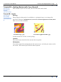
The geology for this project is available as a 'geological map', in an image file.
Located in directory: GeoModeller\tutorial\CaseStudyB\TutorialB1\Data
There are two files available
FieldGeology.jpg
FieldGeologyWithCOVER.jpg
In this tutorial we use the covered geology.
Location
The tutorial gives details of the extents when required.
Stratigraphy
You need to input the stratigraphy for the project area, and also give names to the
two faults. The tutorial gives details when required.
Contents Help | Top
© 2013 BRGM & Desmond Fitzgerald & Associates Pty Ltd
| Back |
GeoModeller User Manual
Contents | Help | Top
Tutorial case study B (Antonio’s map)
3
| Back |
B1 Stage 1—Starting the project
Parent topic:
Tutorial B1—
Getting Started
with Case Study
B
B1 Stage 1—Steps
1
From the main menu choose Project > New OR
From the Project toolbar choose New
Select the project directory from the file chooser.
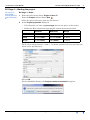
2
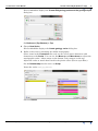
In the Project properties dialog box:
•
Give the project a name (CaseStudyB) (do not use spaces in the name)
•
Define the East, North and Z geographic extents based on the table.
Minimum
Maximum
Range
East
10 000 (Xmin)
14 000 (Xmax)
4 000 m
North
20 000 (Ymin)
23 700 (Ymax)
3 700 m
RL (Z)
–1 000 (Zmin)
100 (Zmax)
1 100 m
The Z values range between –1000 ('–' for below ground) and 100 ('up in the air',
100 m above ground level).
Choose OK.
3D GeoModeller displays the Project creation successful dialog box.
Contents Help | Top
© 2013 BRGM & Desmond Fitzgerald & Associates Pty Ltd
| Back |
GeoModeller User Manual
Contents | Help | Top
3
Tutorial case study B (Antonio’s map)
4
| Back |
Choose Define as a horizontal plane.
For this project, use a 'horizontal topography' at zero elevation.
Give it a name: Map_DTM.
4
Save the project with a new name and location away from the 3D GeoModeller
installation folders.
From the main menu choose Project > Save As OR
From the Project toolbar choose Save As
Press CTRL+SHIFT+S.
OR
The 'save as' operation is unusual. When you specify a project name you are
actually specifying a folder name. 3D GeoModeller saves the project as an *.xml
(with the same name as the directory) in that directory, along with all associated
or referenced files.
Note that a completed version of this tutorial is available as
GeoModeller\tutorial\CaseStudyB\TutorialB1\Completed_project\
TutorialB1.xml. Do not overwrite it.
Contents Help | Top
© 2013 BRGM & Desmond Fitzgerald & Associates Pty Ltd
| Back |
GeoModeller User Manual
Contents | Help | Top
Tutorial case study B (Antonio’s map)
5
| Back |
B1 Stage 2—Enter stratigraphy, define stratigraphic order, define onlap or erode
Parent topic:
Tutorial B1—
Getting Started
with Case Study
B
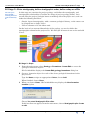
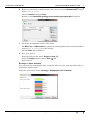
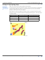
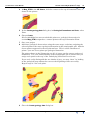
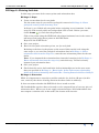
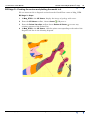
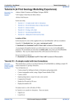
In this stage we examine the project geology, and define the stratigraphy, and
stratigraphic relationships. Consider the image of project geology (below). Let's
assume that the project geologist knows something about the project area, and can
make the following decisions:
•
Simple, layered stratigraphy, with a common geological history, so the strata can
be grouped into a single 'series'.
•
'Green' is known to be the oldest unit.
On the basis of our assumed knowledge of the geology, we need to define the
stratigraphic column for the project area. We shall put all strata in one series and add
'Cover'.
B1 Stage 2—Steps
1
From the main menu, select Geology > Formations: Create-Edit to create the
'geological formation objects'
3D GeoModeller displays the Create-Edit geology formations dialog box
2
Create a 'formation object' for each of the above geological formations in the
project area.
Type the Name, assign an appropriate Colour, choose Add.
When finished, choose Close.
3
When you choose Close, 3D GeoModeller may display the New formation
creation tip box.
Choose Yes, start Stratigraphic Pile editor.
If this box does not appear, from the main menu, choose Stratigraphic pile: Create
or edit.
Contents Help | Top
© 2013 BRGM & Desmond Fitzgerald & Associates Pty Ltd
| Back |
GeoModeller User Manual
Contents | Help | Top
Tutorial case study B (Antonio’s map)
6
| Back |
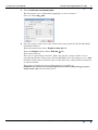
3D GeoModeller displays the Create-Edit geology series and the geological pile
dialog box.
Set Reference (Top-Bottom) to Top.
4
Choose New Series.
3D GeoModeller displays the Create geology series dialog box.
5
Define a first series containing the folded stratigraphy:
Select items in the Formations list, and use the across arrow buttons to add
formations to the Series. You can use the Move up and Move down to adjust the
stratigraphic order—oldest strata at the bottom, and youngest at the top.
Adjust the order to match that listed in the picture above (Green up to Blue).
Set the Relationship for this series to Onlap.
Name the series Case_B_Series.
Choose Commit.
Contents Help | Top
© 2013 BRGM & Desmond Fitzgerald & Associates Pty Ltd
| Back |
GeoModeller User Manual
Contents | Help | Top
6
Tutorial case study B (Antonio’s map)
7
| Back |
Define a second series containing the unit 'Cover', also with Relationship = Onlap.
Call it Case_B_Cover.
Choose Commit and then Close.
Return to the Create-Edit geology series and the geological pile dialog box.
7
Check the stratigraphic order of the series.
Use Move up and Move down to adjust the stratigraphic order so that the oldest
series (Case_B_Series) is at the bottom.
Choose Close when finished.
8
Save your project.
From the main menu choose Project > Save OR
From the Project toolbar choose Save
Press CTRL+S.
OR
B1 Stage 2—Other activities
You can view the stratigraphic pile, check the order of series, and check the order of
formations within series.
From the main menu choose Geology > Stratigraphic Pile: Visualise.
Contents Help | Top
© 2013 BRGM & Desmond Fitzgerald & Associates Pty Ltd
| Back |
GeoModeller User Manual
Contents | Help | Top
Tutorial case study B (Antonio’s map)
8
| Back |
B1 Stage 3—Enter faults, define fault-strata relationship, define fault-fault
relationship
Parent topic:
Tutorial B1—
Getting Started
with Case Study
B
In the geology map there are two faults, called ENE and WNW. In this stage we
specify them in the project.
B1 Stage 3—Steps
1
Create an object for each fault. From the main menu, choose Geology > Faults:
Create or Edit. 3D GeoModeller displays the Create-Edit faults dialog box.
2
Create a fault object each of the two faults in the project area.
Name
Colour
ENE
Green
WNW
Blue
Input the Name, assign an appropriate Colour, choose Add.
When finished, choose Close.
Contents Help | Top
© 2013 BRGM & Desmond Fitzgerald & Associates Pty Ltd
| Back |
GeoModeller User Manual
Contents | Help | Top
3
Tutorial case study B (Antonio’s map)
9
| Back |
When you select Close you may be prompted to start the ‘link faults with series
editor’. Choose ‘Yes, start link Faults With Series editor’. If the dialog does
not appear start the editor from the main menu. Choose Geology > Faults: Link
faults with series.
3D GeoModeller will display the Link faults with series dialog box.
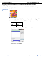
4
You can specify that faults affect some series within the stratigraphic pile, but
have no impact on other series. Define the series-fault relationships.
Check the cells in the table so that 'Case_B_Series' is linked with both the ENE
and WNW faults.
Do not link the Case_B_Cover series to the faults.
Choose OK.
5
You can define a fault as 'stopping on' some other fault. Define the 'fault-fault
relationship'.
From the main menu, choose Geology > Faults: Link faults with faults.
3D GeoModeller dsplays the Link faults with faults dialog box.
Check the boxes to specify that the WNW fault 'stops on' the ENE fault.
Choose OK.
6
Contents Help | Top
Save your project.
© 2013 BRGM & Desmond Fitzgerald & Associates Pty Ltd
| Back |
GeoModeller User Manual
Contents | Help | Top
Tutorial case study B (Antonio’s map)
10
| Back |
B1 Stage 4—Import geology image
Parent topic:
Tutorial B1—
Getting Started
with Case Study
B
There are several ways to input geological observations.
We shall simulate going into the field to make geological observations by importing a
geological map with cover. There are extensive areas of cover, but some bedrock
geology is exposed and able to be mapped.
After import we shall georegister the image so that it corresponds with the project.
The image has four registration points for aligning with the project. We only need to
use three of them.
Contents Help | Top
Registration point
X coordinate (East)
Y coordinate (North)
Top left
10000
23700
Top right
14000
23700
Bottom right
14000
20000
© 2013 BRGM & Desmond Fitzgerald & Associates Pty Ltd
| Back |
GeoModeller User Manual
Contents | Help | Top
Tutorial case study B (Antonio’s map)
11
| Back |
B1 Stage 4—Steps
1
In the 2D Viewer select Map_DTM.
From the Map_DTM shortcut menu choose Image manager.
3D GeoModeller displays the Image manager.
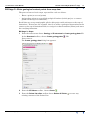
2
Choose New. 3D GeoModeller displays the Edit and align image dialog box.
Choose Browse and open:
GeoModeller\tutorial\CaseStudyB\TutorialB1\Data\
FieldGeologyWithCOVER.jpg
Contents Help | Top
© 2013 BRGM & Desmond Fitzgerald & Associates Pty Ltd
| Back |
GeoModeller User Manual
Contents | Help | Top
Tutorial case study B (Antonio’s map)
12
| Back |
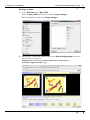
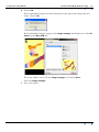
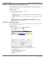
If your image has three or more points for which you know the geographical
coordinates, you can use the Edit and align image dialog box to georegister the
image in your project. After georegistration, each point in the image corresponds
to the correct location in the 3D GeoModeller project.
On the left is a copy of the image you have opened. On the right is a copy of the
image as registered in the 3D GeoModeller project.
The left panel has three movable alignment points. You will move them to the
correspond with the three known registration points in the image.
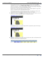
3
Enlarge the image in the Image panel and move the view to the top left corner so
that you can see the registration point and alignment point 1.
Drag alignment point 1 to exactly align with the registration point in the image.
4
Contents Help | Top
Enter the coordinates of this point (10000, 23700) in the table at the bottom of the
dialog box as u and v for alignment point 1.
© 2013 BRGM & Desmond Fitzgerald & Associates Pty Ltd
| Back |
GeoModeller User Manual
Contents | Help | Top
Tutorial case study B (Antonio’s map)
13
| Back |
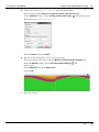
In the Section panel, 3D GeoModeller warps the image to correctly geolocate
this point.
5
Contents Help | Top
Repeat steps 3–4 for the top-right and bottom-right registration points,
corresponding to alignment points 2 and 3.
© 2013 BRGM & Desmond Fitzgerald & Associates Pty Ltd
| Back |
GeoModeller User Manual
Contents | Help | Top
6
Tutorial case study B (Antonio’s map)
14
| Back |
Choose OK.
3D GeoModeller reports the final dimension of the part of the image that it is
using. Choose OK.
3D GeoModeller lists the image in the Image manager and displays it in the 2D
Viewer in the Map_DTM tab.
If it is not visible, select it in the Image manager and choose Show.
Close the Image manager.
7
Contents Help | Top
Save your project.
© 2013 BRGM & Desmond Fitzgerald & Associates Pty Ltd
| Back |
GeoModeller User Manual
Contents | Help | Top
Tutorial case study B (Antonio’s map)
15
| Back |
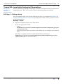
Tutorial B2—Input Initial Geological Observations
Parent topic:
Tutorial case
study B
(Antonio’s map)
We have finished specifying stratigraphy and faults and imported and georegistered a
topography map. Now we are ready to start entering geology observations.
B2 Stage 1—Getting started
You can continue with your version of the project that you completed in Tutorial B1—
Getting Started with Case Study B or open the project that we have prepared, ready
to start this tutorial.
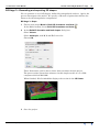
B2 Stage 1—Steps
1
Open the completed project from Tutorial B1.
To use the prepared version:
•
Open:
GeoModeller\tutorial\CaseStudyB\TutorialB1\Completed_project
\TutorialB1.xml
•
Save the project with a new name in the folder you are using for your tutorial
data.
Note that a completed version of this Tutorial B2 is available as
GeoModeller\tutorial\CaseStudyB\TutorialB2\Completed_project
\TutorialB2.xml. Do not overwrite it.
Contents Help | Top
© 2013 BRGM & Desmond Fitzgerald & Associates Pty Ltd
| Back |
GeoModeller User Manual
Contents | Help | Top
2
Tutorial case study B (Antonio’s map)
16
| Back |
(If not already showing) Open Map_DTM in the 2D Viewer and display the geology
map image.
(If the Map_DTM tab is not visible) In the Explorer tree, expand Sections and
select Map_DTM.
From the shortcut menu, choose Open 2D viewer. 3D GeoModeller displays the
section in the 2D Viewer.
(If the topography image is not showing) In Map_DTM in the 2D Viewer, from the
shortcut menu choose the image name to show or hide it OR
Press PAGEUP or PAGEDOWN to show, and END to hide.
Now we can start recording observations of the geology, and so begin building the
3D geological model of this project area.
Contents Help | Top
© 2013 BRGM & Desmond Fitzgerald & Associates Pty Ltd
| Back |
GeoModeller User Manual
Contents | Help | Top
Tutorial case study B (Antonio’s map)
17
| Back |
B2 Stage 2—Enter geological contact points from map view
The process has two basic steps, repeated for each set of data:
•
Enter a point (or a set of points)
•
Assign those points to a specified geological horizon (in this project, as contact
points for the top of a formation).
Recall that we set up stratigraphic pile for this project with reference to the tops of
formations. This means, for example, that if we make a geological observation on the
contact at the top of formation Plum, we assign it to that formation (Plum), and not to
the overlying formation.
B2 Stage 2—Steps
1
From the main menu choose Geology > 2D structural > Create geology data OR
In the Structural toolbar, choose Create geology data
Press CTRL+G.
. OR
The Create geology data dialog box appears.
Contents Help | Top
2
From the 2D Viewer toolbar, choose Create
.
3
From the Points list editor toolbar choose Delete all Points
existing contents of the Points List.
© 2013 BRGM & Desmond Fitzgerald & Associates Pty Ltd
to erase any
| Back |
GeoModeller User Manual
Contents | Help | Top
Tutorial case study B (Antonio’s map)
18
| Back |
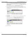
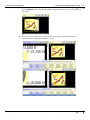
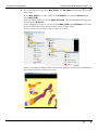
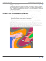
4
In Map_DTM in the 2D Viewer, click the contact at the top of formation Plum, as
shown in the picture.
5
In the Create geology data dialog box, in Geological formations and fonts, select
Plum.
6
Choose Create.
3D GeoModeller has now recorded this point as a geological observation in
section Map_DTM, assigned as a contact point at the top of formation Plum.
7
Save your project
8
Add more geological observations using the same steps, each time assigning the
selected point to the correct geological formation in the stratigraphic pile. Add the
eleven points suggested in the map shown here. This is a bare minimum of
points—just one or two points per geological formation.
The points shown in the illustration are all, of course, on the contact surfaces of
formations. Use your understanding of the stratigraphic pile to ensure that you
assign each point to the ‘top’ of the ‘underlying’ formation in each case.
If you can’t easily distinguish the two shades of grey, you may ‘cheat’ by looking
at the geological map without the cover at the beginning of this case study.
Repeat steps 3–7 for each point.
9
Contents Help | Top
Close the Create geology data dialog box.
© 2013 BRGM & Desmond Fitzgerald & Associates Pty Ltd
| Back |
GeoModeller User Manual
Contents | Help | Top
Tutorial case study B (Antonio’s map)
19
| Back |
B2 Stage 2—Discussion
If you tried to 'compute' the model at this point, there would be nothing to compute!
Why? In fact, it would be possible to 'fit-a-surface' through this minimal number of
points. Without any orientation data, however, it is not possible to decide which side
is 'up' and which is 'down'.
Therefore, GeoModeller will not compute a solution where there is no orientation
data. You must have at least one point of orientation data to determine 'facing'.
B2 Stage 3—Enter orientation data from the map view
Entering orientation data is similar to entering contact points, but you must also
enter the correct azimuth and inclination values.
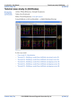
Our project geologist has made the following strike and dip observations:
•
Twelve, related to the strata (shown in white below)
•
Two, indicating that the two faults are vertical (shown in black with thicker
border below)
The geologist has recorded the data as vector directions. 3D GeoModeller also uses
this convention. The azimuth direction is measured from North as per convention.
The dip value can be thought of as 'dip of the strata down from horizontal', but
equally it can be thought of as defining a 'facing vector', having an angle measured
'from vertical' in the direction of the specified dip direction.
Contents Help | Top
© 2013 BRGM & Desmond Fitzgerald & Associates Pty Ltd
| Back |
GeoModeller User Manual
Contents | Help | Top
Tutorial case study B (Antonio’s map)
20
| Back |
B2 Stage 3—Steps
1
From the Structural toolbar, choose Create orientation data
.
In the Create geology orientation data dialog box, check Automatically update
coordinates.
2
From the 2D Viewer toolbar, choose Create
OR press C.
3
From the Points list editor toolbar choose Delete all Points
existing contents of the Points List.
4
In Map_DTM in the 2D Viewer, click the one of the points where strike and dip
have been recorded (For the one shown, values are: 322 and 15).
to erase any
Observe that the coordinates of the point appear in the Create geology
orientation data dialog box.
Contents Help | Top
© 2013 BRGM & Desmond Fitzgerald & Associates Pty Ltd
| Back |
GeoModeller User Manual
Contents | Help | Top
5
Tutorial case study B (Antonio’s map)
21
| Back |
In the Create geology orientation data dialog box:
•
For Geology formations and faults, select Plum.
•
Enter Dip direction: 322.
•
Enter Dip: 15.
•
Choose Apply.
This point has now been recorded as 'an orientation observation in section
Map_DTM, assigned to unit Plum, with a specified (x, y) location, and specified
azimuth and dip values.
6
Save your project.
7
Repeat steps 3–6 for the rest of the points shown in the picture at the beginning of
this stage of the tutorial (shown in white in this tutorial, but in black in the image
that you have imported to the project). Each time, assign the selected point to the
correct geological formation in the stratigraphic pile, and enter the required
azimuth and dip values.
Ignore, for now, the points defining the fault attitude (shown in black in this
tutorial, but not shown in the image).
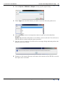
Alternatively: You can import the 13 orientation points from a data file
supplied:
GeoModeller\tutorial\CaseStudyB\TutorialB2\Data
\Orientation_B2.data
From the main menu choose Import > Import 2D data.
Choose Browse, open the file and choose OK.
8
Contents Help | Top
Close the Create geology orientation data dialog box.
© 2013 BRGM & Desmond Fitzgerald & Associates Pty Ltd
| Back |
GeoModeller User Manual
Contents | Help | Top
Tutorial case study B (Antonio’s map)
22
| Back |
B2 Stage 3—Further optional activities
Now that you have entered geology contact observations and some orientation data
defined, 3D GeoModeller can compute and plot the model.
1
From the main menu choose Model > Compute OR
From the Model toolbar choose
Press CTRL+M.
OR
Use these settings:
•
Sections to take into account: All
•
Series to interpolate: All
Choose OK.
2
Select Map_DTM tab in the 2D Viewer.
3
From the main menu choose, choose Model > Plot the model settings OR
From the Model toolbar, choose Plot the model settings
Pess CTRL+D.
OR
Set the parameters:
•
Check Show fill and clear Show lines.
•
Use default values for the other parameters.
Choose OK.
Your results will have something in common with the images provided, but there is
more work to do. We need to specify the faults.
B2 Stage 3—Discussion
Orientation Data in 3D GeoModeller
Orientations are essentially facings (orthogonal to the geological surface, in the
direction of stratigraphic younging).
It is important to record orientations with the correct sense of 'up'; if some of the
orientation data for a formation are incorrectly assigned an upside down facing, then
3D GeoModeller's computation of the potential (or surface) for that formation could be
quite convoluted!
From a topological viewpoint, every surface in 3D GeoModeller has up and down
sides. Therefore, even faults and intrusives must have at least one piece of
orientation data to define this direction.
Contents Help | Top
© 2013 BRGM & Desmond Fitzgerald & Associates Pty Ltd
| Back |
GeoModeller User Manual
Contents | Help | Top
Tutorial case study B (Antonio’s map)
23
| Back |
B2 Stage 4—Entering fault data
In this stage you enter fault contact points and orientation data
B2 Stage 4—Steps
1
Create contact data for the two faults.
Use the same steps as you used for geological contacts in B2 Stage 2—Enter
geological contact points from map view.
In Stage 2, you clicked only one point before assigning it to a formation. In this
step you click several points and assign them all to a fault. Before you start,
choose Create
(C) and clear the points list.
Click a few points along the ENE fault (the almost horizontal one in the centre of
teh image) and assign those points to the ENE Fault.
Repeat for the WNW Fault.
2
Save your project.
3
Enter the two fault orientation points, one for each fault.
Referring to the data in the picture at the start of this tutorial, and using the
same steps as you used for geological orientation data in B2 Stage 3—Enter
orientation data from the map view, enter the two orientation points for the two
faults.
Note: If you imported the orientation data instead of entering it (in B2 Stage 3—
Enter orientation data from the map view), omit this step. You have already
imported your orientation data.
4
Save your project.
5
Check that the series–fault and fault–fault relationships are in the same state
that you specified in B1 Stage 3—Enter faults, define fault-strata relationship,
define fault-fault relationship. in Tutorial B1—Getting Started with Case Study B
B2 Stage 4—Discussion
While it is important to correctly record the attitude of a fault in 3D space (in this
case, vertical), the choice of facing direction for these faults is arbitrary.
It does not matter whether the ENE Fault 'faces' north or south.
3D GeoModeller requires that each surface to be computed has at least one piece of
orientation data. Where you do not supply orientation data, 3D GeoModeller does
not compute a solution and, in the model, the feature will not exist.
Contents Help | Top
© 2013 BRGM & Desmond Fitzgerald & Associates Pty Ltd
| Back |
GeoModeller User Manual
Contents | Help | Top
Tutorial case study B (Antonio’s map)
24
| Back |
Tutorial B3—Compute the Model and Draw a Geology Map
Parent topic:
Tutorial case
study B
(Antonio’s map)
We have already created the project, and completed stratigraphy and faults. In
Tutorial B2—Input Initial Geological Observations we completed all of the simple
data entry. We are now ready to compute the model and view 3D results.
At this point we have a very minimalist geological mapping project:
•
Project East, North & Z extents defined.
•
Topography defined
•
Stratigraphy units defined, and ordered in a stratigraphic pile, and grouped into
'series'
•
Two faults defined
•
Some minimalist geological mapping recorded in the Map_DTM section view.
•
Eleven geological contact points - about one per unit
•
A handful of contact points defining the location of two faults
•
Fourteen orientation data points for selected geology and the two faults
We are ready to 'compute the model' and see what is achieved with this minimalist
mapping work!
Contents Help | Top
© 2013 BRGM & Desmond Fitzgerald & Associates Pty Ltd
| Back |
GeoModeller User Manual
Contents | Help | Top
Tutorial case study B (Antonio’s map)
25
| Back |
B3 Stage 1—Getting started and computing the model
You can continue with your version of the project that you completed in Tutorial B2—
Input Initial Geological Observations or open the project that we have prepared,
ready to start this tutorial.
B3 Stage 1—Steps
1
Open the completed project from Tutorial B2.
To use the prepared version:
•
Open:
GeoModeller\tutorial\CaseStudyB\TutorialB2\Completed_project
\TutorialB2.xml
•
Save the project with a new name in the folder you are using for your tutorial
data.
Note that a completed version of this Tutorial B3 is available as
GeoModeller\tutorial\CaseStudyB\TutorialB3\Completed_project
\TutorialB3.xml. Do not overwrite it.
B3 Stage 2—Computing the model
When 3D GeoModeller computes the model it produces a set of equations from which
it can render pictures of the model.
B3 Stage 2—Steps
1
From the main menu choose Model > Compute OR
From the Model toolbar choose
Press CTRL+M.
OR
In the Compute the model dialog box, set parameters as follows:
Use these settings:
•
Sections to take into account: All
•
Series to interpolate: All
Choose OK.
2
Contents Help | Top
Save your project.
© 2013 BRGM & Desmond Fitzgerald & Associates Pty Ltd
| Back |
GeoModeller User Manual
Contents | Help | Top
Tutorial case study B (Antonio’s map)
26
| Back |
B3 Stage 3—Plotting the model
At this point 3D GeoModeller has computed a model, but the model is simply a set of
equations.
We now want to draw a map of the geology of this project area, based on the computed
3D model. We draw the map in the Map_DTM map view section.
Every map and section is drawn by 'interrogating the model'. 3D GeoModeller
defines an (x, y) mesh across the section view. For each mesh node at point P (x, y, z)
3D GeoModeller asks the model 'what are you ?'. The answer is one of the geological
formations, such as 'Green', or 'Plum'.
Using this information as a starting framework, 3D GeoModeller further
interrogates the model to deduce where it should draw formation contact lines.
The fine-ness or coarseness of this 'mesh' will impact upon the quality of the rendered
output. It also impacts upon the speed of rendering.
B3 Stage 3—Steps
1
Select Map_DTM tab in the 2D Viewer.
2
From the main menu choose, choose Model > Plot the model settings OR
From the Model toolbar, choose Plot the model settings
Pess CTRL+D.
OR
In the Plot the model dialog box, set the parameters:
•
Check Show lines and clear Show fill.
•
Use default values for the other parameters.
Choose OK.
Contents Help | Top
© 2013 BRGM & Desmond Fitzgerald & Associates Pty Ltd
| Back |
GeoModeller User Manual
Contents | Help | Top
Tutorial case study B (Antonio’s map)
27
| Back |
3D GeoModeller displays the plotted model.
B3 Stage 3—Discussion and further exploration
In the Plot the model dialog box, the 'u point' and 'v point' define the degree of
fineness of the mesh used for the initial interrogation of the model.
For this simple model the default values of 50 x 50 are adequate. A model with fine
detail might require a finer mesh. Alternatively, for a quick render, select a coarser
mesh.
•
Experiment with the mesh size (u, v), replotting each time
•
Experiment with the layout options. From the shortcut (right click) menu choose
Display parameters. Turn the various layers of rendered results on and off. If one
layer appears to be hidden under another, turn the display of both off and then
turn on the one at the back first.
•
Experiment with re-plotting the model using Fill and Trend
To erase the display of all model (calculated) data from the model, so that only the
original data remains:
From the main menu choose Model > Erase all model geology OR
From the shortcut menu in the 2D Viewer choose Erase all model geology OR
In the Model toolbar choose Erase all model geology
Contents Help | Top
© 2013 BRGM & Desmond Fitzgerald & Associates Pty Ltd
.
| Back |
GeoModeller User Manual
Contents | Help | Top
Tutorial case study B (Antonio’s map)
28
| Back |
B3 Stage 4—Compute and render: Discussion of result
In this stage we plot the model using lines over the image beneath. We assess its
accuracy and discuss.
B3 Stage 4—Steps
Using the instructions in B3 Stage 3—Discussion and further exploration
1
Erase all model geology
From the main menu choose Model > Erase all model geology OR
From the shortcut menu in the 2D Viewer choose Erase all model geology OR
In the Model toolbar choose Erase all model geology
2
.
Display the image.
In Map_DTM in the 2D Viewer, from the shortcut menu choose the image name to
show or hide it OR
Press PAGEUP or PAGEDOWN to show, and END to hide.
3
Plot the model with lines.
4
Examine the outcome. Are these results OK?
B3 Stage 4—Discussion
The contact contours do honour the sampled points of geology.
The faults are well delineated by several sample points. These are honoured by the
model result.
The orientation data are honoured
The result is not too bad considering the lazy mapping job that we have done! Those
few points that have been mapped are honoured accurately. Even with these few
points the modelled geology is crudely correct.
Of course, the model is wrong in many places. We know it’s wrong because we can see
in the geology image where it has gone wrong.
Can we do a better geological mapping job on this project area?
The faults are well defined—no further work needed!
Orientation data—we've used all the measurements that are available. No more
needed.
Contents Help | Top
© 2013 BRGM & Desmond Fitzgerald & Associates Pty Ltd
| Back |
GeoModeller User Manual
Contents | Help | Top
Tutorial case study B (Antonio’s map)
29
| Back |
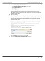
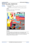
Geological contacts? Although there is extensive cover, we could still improve our
mapping. Taking this tutorial to a logical conclusion, we could end up with a project
with many more observations of the geology, as shown in the following diagram.
What can we expect when we compute the revised model? In Tutorial B4—Add Data,
Recompute, Redraw the Geology Map
Contents Help | Top
© 2013 BRGM & Desmond Fitzgerald & Associates Pty Ltd
| Back |
GeoModeller User Manual
Contents | Help | Top
Tutorial case study B (Antonio’s map)
30
| Back |
Tutorial B4—Add Data, Recompute, Redraw the Geology Map
Parent topic:
Tutorial case
study B
(Antonio’s map)
In this tutorial we add further geological contact data to our project and examine the
resulting model for improvement.
B4 Stage 1—Getting started and computing the model
You can continue with your version of the project that you completed in Tutorial B3—
Compute the Model and Draw a Geology Map or open the project that we have
prepared, ready to start this tutorial.
B4 Stage 1—Steps
1
Open the completed project from Tutorial B3.
To use the prepared version:
•
Open:
GeoModeller\tutorial\CaseStudyB\TutorialB3\Completed_project
\TutorialB3.xml
•
Save the project with a new name in the folder you are using for your tutorial
data.
Note that a completed version of this Tutorial B4 is available in
GeoModeller\tutorial\CaseStudyB\TutorialB4\Completed_project
\TutorialB4.xml. Do not overwrite it.
2
Select Map_DTM tab in the 2D Viewer.
3
Erase all model geology.
4
Hide the image if it is visible.
B4 Stage 2—Importing additional data
Our geologist has supplied more detailed contact data for the site. The data is in an
ASCII file the 3D GeoModeller can import.
B4 Stage 2—Steps
1
Import the data in the file
GeoModeller\tutorial\CaseStudyB\TutorialB4\Data
\TutorialB4.data
Select Map_DTM tab in the 2D Viewer.
From the main menu choose Import > Import 2D data.
Choose Browse and open the file.
Choose OK.
Contents Help | Top
© 2013 BRGM & Desmond Fitzgerald & Associates Pty Ltd
| Back |
GeoModeller User Manual
Contents | Help | Top
Tutorial case study B (Antonio’s map)
31
| Back |
View the new data in the Map_DTM tab of the 2D Viewer.
B4 Stage 2—Discussion
We now have a more complete geological mapping project.
We have defined all of the basics:
•
Project East, North & Z extents
•
Topography
•
Stratigraphy units, ordered in a stratigraphic pile, and grouped into series
•
Two faults
•
And fairly complete geological mapping in the Map_DTM section view
•
About 100 geological contact points
•
Contact points that define the location of two faults
•
Fourteen orientation data points for some geology and the two faults
We are ready to recompute the model and see what we have achieved with this more
complete geological mapping work.
B4 Stage 2—Recomputing and plotting the model
B4 Stage 2—Steps
Repeat the steps in Tutorial B3—Compute the Model and Draw a Geology Map.
1
Compute the model with all components selected
Carry out the steps in B3 Stage 2—Computing the model
2
Plot the model with lines on Map_DTM section.
Carry out the steps in B3 Stage 3—Plotting the model
Contents Help | Top
© 2013 BRGM & Desmond Fitzgerald & Associates Pty Ltd
| Back |
GeoModeller User Manual
Contents | Help | Top
Tutorial case study B (Antonio’s map)
32
| Back |
B4 Stage 3—Compute and render, discuss result
In this stage we plot the model using lines with the image beneath. We assess its
accuracy and discuss.
B4 Stage 3—Steps
Using the instructions in B3 Stage 3—Discussion and further exploration
1
Erase all model geology
2
Display the image.
3
Plot the model usig lines.
4
Examine the outcome. Are these results OK?
B4 Stage 3—Discussion
Quality of the model
The model contact lines honour the sampled points of geology.
The model honours the orientation data.
A 3D GeoModeller model cannot claim to be the 'correct answer'! At best, it can only
claim to be a model that is ‘consistent with the observed geological observations'.
Certainly the model in this case is in good agreement with the exposed (mapped)
geology.
A large portion of the map generated above is 'interpolation'. For this project we
actually know what is under the cover.
Contents Help | Top
© 2013 BRGM & Desmond Fitzgerald & Associates Pty Ltd
| Back |
GeoModeller User Manual
Contents | Help | Top
Tutorial case study B (Antonio’s map)
33
| Back |
The image without cover
Recall that we have a map without the cover, so we can compare our results with it.
The map is in the file GeoModeller\tutorial\CaseStudyB\TutorialB4\Data
\FieldGeology.jpg
Admittedly this is a simple geology map, with broad predictable folding, but the
interpolation from about 20% outcrop has achieved a good result.
You could import and georegister this image in the project. Use the instructions in
B1 Stage 4—Import geology image. Note that, if there are several images in a
section, the keystrokes PAGEUP and PAGEDOWN enable you switch between the
available images.
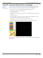
Viewing the model with trend lines
The following illustration is of the computed 'potential' for this series (plotted using
the Show trend lines option. Observe:
Contents Help | Top
•
How the iso-potentials honour the orientation data and the trends of the exposed
geological contacts, and then
•
How they provide the basis for the interpolation of the contacts beneath cover.
© 2013 BRGM & Desmond Fitzgerald & Associates Pty Ltd
| Back |
GeoModeller User Manual
Contents | Help | Top
Tutorial case study B (Antonio’s map)
34
| Back |
Tutorial B5—Cross sections, Shapes and Other Model Products
Parent topic:
Tutorial case
study B
(Antonio’s map)
In this tutorial we:
•
Create a cross section and view the model in it
•
Calculate and export the 3D model in Virtual Reality Modelling Language
(VRML) and view it on a web page
B5 Stage 1—Getting started
You can continue with your version of the project that you completed in Tutorial B4—
Add Data, Recompute, Redraw the Geology Map or open the project that we have
prepared, ready to start this tutorial.
B5 Stage 1—Steps
1
Open the completed project from Tutorial B4.
To use the prepared version:
•
Open:
GeoModeller\tutorial\CaseStudyB\TutorialB4\Completed_project
\TutorialB4.xml
•
Save the project with a new name in the folder you are using for your tutorial
data.
Note that a completed version of this Tutorial B5 is available in
GeoModeller\tutorial\CaseStudyB\TutorialB5\Completed_project\T
utorialB5.xml. Do not overwrite it.
2
Contents Help | Top
Select Map_DTM tab in the 2D Viewer.
© 2013 BRGM & Desmond Fitzgerald & Associates Pty Ltd
| Back |
GeoModeller User Manual
Contents | Help | Top
Tutorial case study B (Antonio’s map)
35
| Back |
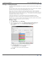
B5 Stage 2—Creating the secton and plotting the model in it
We are interested in a diagonal section from the North West corner of Map_DTM.
B5 Stage 2—Steps
Contents Help | Top
1
In Map_DTM in the 2D Viewer, display the image of geology with cover.
2
From the 2D Viewer toolbar, choose Create
3
From the Points list editor toolbar choose Delete all Points
existing contents of the Points List.
4
In Map_DTM in the 2D Viewer, click the points corresponding to the ends of the
diagonal red line in the folowing diagram
OR press C.
© 2013 BRGM & Desmond Fitzgerald & Associates Pty Ltd
to erase any
| Back |
GeoModeller User Manual
Contents | Help | Top
5
Tutorial case study B (Antonio’s map)
36
| Back |
Create the section Case_B_Section1 from the points trace
Choose menu option Section > Create a section from its trace OR
on the Section toolbar, choose Create section from trace
OR choose CTRL+T.
Enter the name Case_B_Section1.
Choose Create and then Close.
6
Plot the model using fill in this new section view
From the main menu choose, choose Model > Plot the model settings OR
From the Model toolbar, choose Plot the model settings
Pess CTRL+D.
OR
Check Show fill and clear Show lines.
Choose OK.
7
Contents Help | Top
Save the project.
© 2013 BRGM & Desmond Fitzgerald & Associates Pty Ltd
| Back |
GeoModeller User Manual
Contents | Help | Top
Tutorial case study B (Antonio’s map)
37
| Back |
B5 Stage 3—Generating and exporting 3D shapes
We can generate a set of 3D shapes, defined by triangulated surfaces. Again, the
process interrogates the model. We specify a 3D mesh of points that defines the
fineness for the triangulation computation.
B5 Stage 3—Steps
1
Choose main menu Model > Build 3D formations and faults OR
In the Model toolbar choose Build 3D formations and faults
2
In the Build 3D formation and fault shapes dialog box:
Select Volume
Select Anistropic, with X, Y and Z all set to 50.
Choose OK.
These dimensions yield a 50m x 50m x 50m resolution for this project.
The process takes about three minutes for this simple model on a 2.4 GHz
computer with 512 Mb RAM
When finished, 3D GeoModeller displays the results in the 3D Viewer.
3
Contents Help | Top
Save the project.
© 2013 BRGM & Desmond Fitzgerald & Associates Pty Ltd
| Back |
GeoModeller User Manual
Contents | Help | Top
Tutorial case study B (Antonio’s map)
38
| Back |
4
Choose Export > 3D Model > Shapes to bring up the export dialog.
5
Under Type select the file format you wish to save the 3D mesh products in.
6
Choose Browse to select an output file name or type one in the edited box
provided.
NOTE: Most formats will produce several files, one for each unit. In such cases a
ZIP file will be created using the name provided.
Contents Help | Top
7
Once the save is complete you will recieve a message dialog indicating where the
products have been saved.
8
Navigate to the output directory and extract the contents of the ZIP file to ensure
the export was successful.
© 2013 BRGM & Desmond Fitzgerald & Associates Pty Ltd
| Back |
GeoModeller User Manual
Contents | Help | Top
9
Tutorial case study B (Antonio’s map)
39
| Back |
Export VRML files for interactive 3D display in a web browser
NOTE: This is for Micrsoft Internet Explorer only.
After building the shapes, we can generate a set of Virtual Reality Modelling
Language (VRML) files for interactive web display. The process takes about
thirty seconds for this 2.4 MHz PC with 512 Mb RAM.
From the main menu choose Export > Export 3D model > VRML project website.
Specify a folder for your files. 3D GeoModeller places a .zip file in that folder,
containing the VRML web pages.
B5 Stage 3—Solutions provided
•
We supply a completed version of the VRML website, according to the instructions
in this tutorial, in your 3D GeoModeller installation folders. Its path is
GeoModeller\tutorial\CaseStudyB\TutorialB5\
Completed_VRML_Site. Do not overwrite these files.
•
We also provide a high-resolution resolution version. We generated it from shapes
defined with 10 m vertical resolution, and 25 m horizontal resolution. The finer
vertical resolution is more suited to the thin layers of this model. You can
download this in a .zip file (VRML_10mZ_25mXY_Resolution.zip) from the 3D
GeoModeller website www.geomodeller.com.
B5 Stage 4—Viewing the VRML web pages
Before viewing the VRML pages, you need to:
•
Ensure that you have a VRML viewer plug-in for your browser.
•
Unzip the files into folders.
To save time in this exercise, we have generated a relatively coarse-grained (50 m x
50 m) set of shapes. Our output looks OK, but, in a production enviromment, you
may require finer definition.
B5 Stage 4—Steps
1
To view the VRML interactive display:
2
If you do not have a VRML viewer, install one on your computer.
We have tested and used the Blaxxun Contact VRML plug in for Microsoft
Internet Explorer. It enables you to view and interact with web-ready VRML files
in a standard web browser. You can obtain this from the following download:
•
3
ftp://ftp.intrepid-geophysics.com/pub/geomodeller/vrml/blaxxunContact53.exe
Open the .zip file that 3D GeoModeller created. Unzip it into a folder of your
choice. Ensure that the Use folder names option is checked.
The VRML site consists of the following files and folders:
4
•
File index.html for launching the site
•
Folder HTML with various VRML display control files
•
Folder VRML with the geology shape files
Open the file index.html using Microsoft Internet Explorer.
If Microsoft Internet Explorer is your default browser, you can just double click
index.html.
If you have several browsers and Microsoft Internet Explorer is not your default
browser, use Open With from the shortcut (right click) menu in Windows Explorer
or My Computer to launch it.
Contents Help | Top
© 2013 BRGM & Desmond Fitzgerald & Associates Pty Ltd
| Back |
GeoModeller User Manual
Contents | Help | Top
Tutorial case study B (Antonio’s map)
40
| Back |
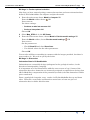
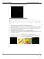
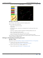
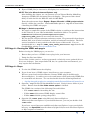
Depending on your security settings, you may need to allow blocked content. Your
browser may display a warning as shown below. Generally you need to right click
the Information Bar near the top of the window and choose Allow Blocked
Content. This permits the browser to load the rest of the VRML data.
The browser displays the web page with an empty display area.
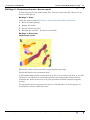
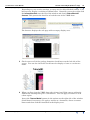
5
Check some or all of the geology formation check boxes on the left side of the
screen. You can also check the check boxes for display of axes as a reference
frame.
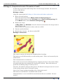
6
When you first view the VRML data, the colours just fill the spaces uniformly,
without the shading that gives a 3D illusion. You can apply a texture to each
colour region.
Locate the Texture Model buttons in the options on the right side of the window
(Scroll down if necessary). To apply a texture to a formation, choose a texture
button and then click the formation in the display area.
Contents Help | Top
© 2013 BRGM & Desmond Fitzgerald & Associates Pty Ltd
| Back |
GeoModeller User Manual
Contents | Help | Top
Tutorial case study B (Antonio’s map)
41
| Back |
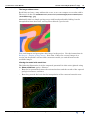
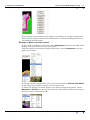
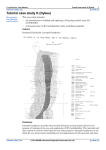
You can rotate, move and reset the display, and change its vertical exaggeration.
This tutorial only has room for brief instructions. Consult the Blaxxun Contact
user manual for full details.
B5 Stage 4—Blaxxun Contact controls
Contents Help | Top
•
To select 2D or 3D display, select one of the Viewpoints buttons at the right of the
display area (scroll to reveal if necessary) OR
From the display area shortcut (right click) menu, choose Viewpoints > and the
option you require.
•
To change vertical exaggeration: select one of the buttons in Vertical Scale Model
at the right of the window (scroll to reveal if necessary).
•
To rotate the display: from the display area shortcut (right click) menu, choose
Movement > Examine (or press CTRL+SHIFT+E). Drag with the left mouse button
to rotate (mouse pointer shows E).
© 2013 BRGM & Desmond Fitzgerald & Associates Pty Ltd
| Back |
GeoModeller User Manual
Contents | Help | Top
Tutorial case study B (Antonio’s map)
42
| Back |
•
To move the display: from the display area shortcut (right click) menu, choose
Movement > Slide (or press CTRL+SHIFT+S). Drag (gently) with the left mouse
button in the opposite direction to the desired movement (mouse pointer shows S).
This may take some practice. If the display disappears, reset it using one of the
Viewpoints buttons.
•
To view the Blaxxun Contact on-line help manual: from the from the display area
shortcut (right click) menu, choose Help > Online Manual. The manual appears in
a new window.
There are further options for rotating, panning and zooming in the shortcut (right
click) menu.
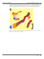
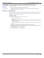
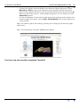
Here is an illustration of another VRML model display.
You have now successfully completed Tutorial B
Contents Help | Top
© 2013 BRGM & Desmond Fitzgerald & Associates Pty Ltd
| Back |