1
CALIFORNIA PATH PROGRAM
INSTITUTE OF TRANSPORTATION STUDIES
UNIVERSITY OF CALIFORNIA, BERKELEY
The NETCELL simulation package:
Technical description
Randall Cayford, Wei-Hua Lin,
Carlos F. Daganzo
University of California, Berkeley
California PATH Research Report
UCB-ITS-PRR-97-23
This work was performed as part of the California PATH program of the University
of California, in cooperation with the State of California Business, Transportation,
and Housing Agency, Department of Transportation; and the United States
Department of Transportation, Federal Highway Administration.
The contents of this report reflect the views of the authors who are responsible for
the facts and the accuracy of the data presented herein. The contents do not
necessarily reflect the official views or policies of the State of California. This report
does not constitute a standard, specification or regulation.
May, 1997
ISSN 1055-1425
The NETCELL Simulation Package:
Technical Description*
Randall Cayford
Wei-Hua Lin
and
Carlos F. Daganzo
Department of Civil Engineering and
Institute of Transportation Studies
University of California, Berkeley, CA 94720-1720
Abstract
This report describes the NETCELL simulation package. NETCELL is a freeway
network simulation program based on the cell transmission model which captures
the dynamic evolution of multicommodity traffic over a freeway network with
three-legged junctions in a way that is consistent with the hydrodynamic theory of
highway traffic. NETVIEW is a graphical postprocessor for viewing NETCELL
output files.
This document discusses implementation of the programs in detail,
including the cell representation for a freeway network with three-legged junctions,
data and file structures, inputs and outputs, and some key algorithms developed to
model traffic progression in junctions. The memory and computational time
requirements for the program are also estimated. An example for a small network
with a single origin, two destinations, and a single diverge junction is included.
This report also includes a userÕs guide to the NETVIEW program.
The NETCELL program is based on a prototype program written in 1994. This
version incorporates some enhancements to the model and memory handling
improvements to allow NETCELL to model very large networks. This version of the
NETCELL program should be useful for use as a research and engineering tool.
Keywords: traffic simulation, traffic flow model, transportation network
traffic congestion management, dynamic traffic assignment.
ii
Executive Summary
This research report provides a technical description of a computer simulation
package, NETCELL, which was designed as a research tool for studying traffic flow
over a large scale network. NETCELL was developed based on the cell transmission
model, a multicommodity traffic flow model especially powerful in capturing the
transient behavior of freeway congestion, such as the formation, propagation, and
dissipation of queues. In addition to the technical description of the internal
simulation engine, the report also details the installation of the package, input
requirements, computational and memory requirements, and limitations. Thus, it
can serve as a user guide as well.
The NETCELL simulation package consists of two components, NETCELL, the
simulation model itself, and NETVIEW, a graphical postprocessor for displaying
output files from NETCELL.
NETCELL is a macroscopic simulation program in which vehicle quantities are
treated as continuous variables. Vehicles are advanced in a way consistent with the
hydrodynamic theory of traffic flow. Unlike most existing traffic models, NETCELL
preserves rigorously the first-in-first-out (FIFO) discipline for multicommodity
network traffic flows. This unique feature is critical for studying freeway ramp
metering and other control strategies, and for evaluating the performance of these
strategies. The input of NETCELL consists of four parts describing the network
geometry, the routing information, any incidents, and the Origin-Destination
inputs. In addition to the traditional input parameters, NETCELL also allows a userspecified piecewise linear flow-density relationship. This feature could enhance the
realism in modeling wave propagation on freeways.
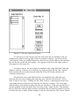
NETVIEW is a graphical windowing program and is available for two platforms, the
Apple Macintosh, and Microsoft Windows. The output of NETCELL can be
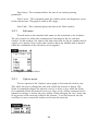
manipulated in NETVIEW with four display windows and four menus. The
windows are the network window, which displays a graphical representation of the
network, the arc selection window, which allows the user to select and deselect the
arcs which are used to calculate results, the curve window, which displays flow-time
curves for the selected arcs, and the table window, which displays the cumulative
counts and other information for the selected arcs. The cumulative counts at userspecified locations are not available as outputs in other existing traffic simulation
programs.
The NETCELL simulation package provides a platform for evaluation of ITS
improvements, environmental impacts, and dynamic control strategies. It holds
promise for the study of dynamic traffic assignment, real time travel information,
and other areas in traffic flow modeling where a proper representation of physical
queues is of paramount importance.
iii
Table of Contents
Part 1:
NETCELL technical description
1
Introduction
1
2
Glossary of Terms
2
3
Cell Representation and Data Structures
3.1 The Network Representation
3.2 The Traffic Flow Representation
3.3 Event Representation
4
The Simulation Algorithm;
Memory and Computations Time Requirements
4.1 The Simulation Algorithm
4.2 Limitations, Memory and Computational
requirements
5
4
5
8
10
11
11
13
File Structure; Input and Output Processes
The Input File
Ouputs
15
15
23
6
An Example Network
25
Part 2:
NETVIEW UserÕs Guide
5.1
5.2
7
Introduction to NETVIEW
28
8
Installing the NETCELL simulation package
8.1 Installation on the Macintosh
8.2 Installation under windows
28
28
28
9
10
Running NETCELL
29
Running NETVIEW
10.1 NETVIEW display windows
10.2 NETVIEW menus
30
31
35
11
References
38
12
Appendices
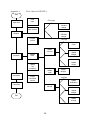
Flowchart for NETCELL
39
39
1
iv
2
3
4
5
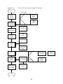
Flowchart for Update Straight
Flowchart for Update Diverge
Flowchart for Update Merge
Sample Input File for the Example
v
40
41
42
43
List of Figures
1
2
3
4
5
6
7
8
9
10
11
12
13
14
15
16
17
18
19
Assumed flow-density relationship
Generalized flow-density relationship
Cell Type specifications
Merge and Diverge Cells in a Junction
User-specified flow-density relationship
Trapezoidal q-k curves with wave speed
greater than the default value
The Computation of Cell Travel Time Ti(t)
Locataions to Take Cumulative Counts
Roadway Geometry for the Example
Q-K Relationship for Every Arc in the Example
Travel Time Ti(t) For Arc 1 At Time t
The Network Window
The Arc Selection Window
The Curve Window
The Table Window
The File Menu
The Edit Menu
The Options Menu
The Window Menu
vi
5
6
7
8
10
19
24
25
25
27
27
32
33
34
35
35
36
36
37
1
Introduction
This report describes the NETCELL simulation package --- a pair of computer
programs that implement the Òcell transmission modelÓ (Daganzo, 1994, 1994a)
programmed in C. The cell transmission model describes the dynamic evolution of
multicommodity traffic over a freeway network with three-legged junctions in a
way that is consistent with the hydrodynamic theory of highway traffic. As such,
NETCELL is a purely macroscopic model in which vehicle quantities are treated as
continuous variables. Thus, in this report the words Ònumber of vehiclesÓ should
always be interpreted as designating a real number.
The NETCELL program is based on a prototype program written in 1994 (Lin,
Daganzo, 1994). This version incorporates some enhancements to the model and
memory handling improvements to allow NETCELL to model very large networks.
A graphical postprocessor has been written as a companion to the simulation
model. Further testing and verification of the basic model has been done since the
prototype was developed. Additional error checking has been also added to
NETCELL. While the prototype was sufficient to show proof of concept and to
confirm the validity of the theoretical model, this version of the NETCELL program
should be useful as a research and engineering tool.
The NETCELL simulation program can handle networks with three-legged
junctions, as described in the theory, and includes a graphical postprocessor,
NETVIEW, for viewing the simulation results. Some error checking for syntax
errors in input data entry is done but checking on logic errors has been purposely
left out of the program, leaving room for the user to explore applications beyond the
limitations of the program. The size of network which can be modeled is limited
primarily by the amount of available memory. Program limitations are discussed in
the section on computational requirements below. The simplicity of the theory has
allowed us to develop an efficient code, with easily verified building blocks.
Formulas are estimated for run time and memory usage.
Part 1 of this report describes the NETCELL program in detail, including its
input and output files. The postprocessor program, NETVIEW, is described in part 2:
the NETVIEW User's Guide. As a prelude to our presentation, the next section
provides a glossary of terms. Section 3 covers the internal structure of the program.
It describes the cell representation of a freeway network and the strategy for storing
all the data in the memory. Section 4 describes the simulation algorithm and its
memory and computational time requirements. Section 5 describes the file
structure, the input and output processes for the program, and section 6 provides a
simple example. Sections 7 through 10 discuss the installation and running of the
programs and the interface of the NETVIEW viewer program.
1
2
Glossary of Terms
The following is a set of terms frequently used in this report or in the
program NETCELL and their definitions. The symbol associated with the term is
included in the parenthesis.
Arc (k) a homogenous roadway segment without entrances or exits, characterized by
its length (miles), free-flow speed (mph), jam density (vpm), and maximum flow
(vph).
Cell (i) the smallest component of the network in the cell transmission model,
representing section of an arc that is covered in the time between clock ticks (δ time
units) at the arc's free flow speed. (Although longer cells could be used, this degrades
the accuracy of the simulation and is not allowed in this version of NETCELL.)
Cell length (li) the same for all the cells in one arc, this distance (meters) should be
covered in one clock step δ at the arc's free flow speed.
Cell occupancy (ni(t)) a non-negative real valued state variable, indicating the
number of vehicles in cell i at time t.
Clock tick time instant t, at which the inbound flow, outbound flow, and occupancy
of every cell are updated and recorded. The time between clock ticks is d. The
aforementioned flows correspond to the interval [t, t+d)
Cohort (Sdnidt(t)) the number of vehicles residing inside cell i at time t that entered
the cell in the time interval [t,t+δ) for t < t.
Companion cells cells that share the same upstream cell or the same downstream
cell.
Companion links (arcs) (k and ck) links (arcs) that share a common cell (node). Each
link (arc) can have at most one companion link (arc).
Current time (t) same as current clock tick.
Destination zone (d) a single node (or a single cell in cell representation) from
which vehicles leave the network.
Free flow speed (vf,i) a cell-specific value, equal to the free flow speed of the
corresponding arc, vf,k.
Inbound flow (yi'(t)) a cell-specific value, indicating the number of vehicles entering
2
cell i in the time interval [t, t+δ). This quantity is also defined for links.
Links connectors between cells.
Maximum occupancy (Ni(t)) a cell-specific and time-specific constant, representing
the maximum number of vehicles that can be held in cell i at time t; it is the product
of the jam density and the cell length, δvf,i.
Maximum throughput (Qi(t)) a cell-specific and time-specific constant, representing
the maximum number of vehicles that can flow in or out of cell i in one clock step;
it is the product of the maximum flow of the arc in which the cell resides and the
clock step δ.
Merge priority coefficient (pk(t) and pck(t)) input parameters for arc k and its
companion arc ck at a merge junction, specifying the fractions of vehicles merging
from each approach when the supply of vehicles from both approaches exceeds what
can be accommodated. (pk(t) + pck(t) = 1.)
Origin zone a single node (or a single cell in cell representation) where traffic
demands are generated and released into the network.
Outbound cell flow (yi''(t)) a cell-specific value, indicating the number of vehicles
leaving cell i in the time interval [t, t+δ).
Packet (nidt(t)) a cell-specific value, indicating the real valued number of vehicles in
cell i at time t that are headed for the same destination d, and have entered the cell
in the same time interval [t,t+δ) for t < t.
Route choice coefficient (bdk(t) and bdck(t)) destination- and time-specific parameters
for the companion arcs of a diverge junction, k and ck, specifying the proportions in
which nidt(t) is split at the diverge in time interval [t,t+δ): (bdk(t) + bdck(t) = 1.)
Transfer size threshold (ε) an input parameter specifying the smallest cohorts
transferable from cell to cell in the program. Amounts under this threshold are not
transferred. This parameter is used by the program to prevent the proliferation of
cohorts without introducing appreciable error.
Travel time (T i(t) or Tk(t)) the time it takes to traverse cell i (or arc k) for vehicles
entering the cell (the arc) at time t.
Wave coefficient (α) a dimensionless constant representing the ratio of the
backward moving wave speed to the free flow speed.
3
3
Cell Representation and Data Structures
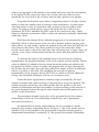
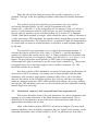
Consider a freeway network represented in the conventional way as a graph
with a set of directed arcs k, a set of nodes, and some connectivity information. Each
arc of this graph is associated with some key physical descriptors of the road segment
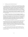
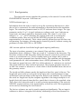
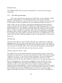
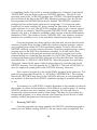
it represents. These include the segment's length dk and four parameters (free-flow
speed vf,k, maximum flow (or capacity), qm,k, jam density, kj,k, and a calculated
backward wave speed, wk) that jointly describe a triangular flow vs. density diagram
as that of Figure 1. (These descriptors are assumed to be given in some consistent
system of units; e.g. meters and seconds, miles and hours...). The user has the option
to specify an alternate wave speed which would define a trapeziodal flow vs. density
diagram, see Figure 6. Figure 1 represents a default case, although we will see later
that a more general flow density relationship, such as those shown in Figures 2 and
6, can also be specified.
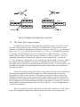
Under the cell representation of a network, a three-legged cell represents
either a ÒmergeÓ or ÒdivergeÓ junction. Two priority coefficients are defined for each
merge; they indicate the fraction of vehicles that enter the node from each approach
when queues exist on both approaches. We also assume that two destination-specific
route choice constants (usually 0 or 1) are defined for each exit to a diverge; they
indicate the fraction of vehicles with destination d that take the corresponding exit.
Although the priority and route choice coefficients can vary with time, in the
current version of the NETCELL program, they are assumed to be time-invariant.
This restriction may be relaxed some time in the future.
In the cell transmission model, the conventional network representation just
described needs to be altered. Each arc should be partitioned into sections, called
ÒcellsÓ, which should be traversed in one simulation clock step under free-flow
conditions [1]. Cells are then viewed as additional network nodes, themselves
connected by additional arcs. (To avoid any confusion, the arcs between cells are
called ÒlinksÓ.) In the cell representation, the roadway characteristics are attached to
cells, and not to links as would be conventional. The cell characteristics are uniquely
determined by the clock step δ as is shown below.
For a clock step of δ time units, the length of each cell is defined to be δvf,k.
The number of cells used for arc k is the positive integer, m k, that is closest to dk/δ
vf,k. This introduces a small change in the effective length of the arc which can be
reduced by reducing δ.
4
Flow
qm,k
V f,k
-W k
k j,k
k 0,k
Density
Figure 1: Assumed flow-density relationship
The parameter qm,k becomes a cell-specific constant that denotes the
maximum number of vehicles that can either enter or exit the cell in one clock step.
For a cell i of arc k the constant is Q i = δqm,k. This constant can be changed in the
middle of a simulation run if we specify that an incident reduces the capacity at a
point in the arc that corresponds to the cellÕs location.
The parameter kj,k becomes a cell-specific constant denoting the maximum
number of vehicles that can be present in a cell at any given time. For cell i of arc k,
the constant is: N i = kj,k δv f,k.
The parameter w k is represented in the cell transmission model by the
dimensionless cell-specific constant αi = w k /vf,k, where cell i is assumed to be in arc
k. The default αi for an arc is calculated as δqm,k /(kj,k vf,k-δqm,k).
3.1
The network representation
In this implementation of NETCELL the connectivity of the network is
embedded in the representation of the arcs. In the input file for a simulation run,
the network is described using nodes and connecting arcs. The node information is
used to set up the connections between arcs only and is discarded before the
simulation begins. The arcs themselves are not arcs in the traditional sense of links
connecting nodes but are really just placeholders for information common to the
cells which comprise the arc. The network itself is represented by the list of cells
belonging to each arc.
5
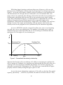
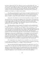
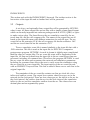
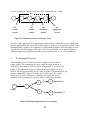
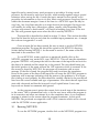
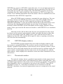
With three legged junctions and more than one cell per arc, cells can only
belong to one of three types: ordinary (type 0), diverge (type 1) or merge (type 2); see
Figure 3. As shown in the figure, ordinary cells are connected to one upstream and
one downstream cell, diverge cells are connected to two downstream cells, and
merge cells to two upstream cells. Diverge cells are the last cells of arcs pointing to a
diverge node, and merge cells the first cells of arcs pointing away from a merge
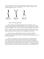
node. This is illustrated in Figure 4, in which each arc is represented by four cells. In
addition, the network must include special cells to represent origins and
destinations. These must be connected by a single link to an ordinary cell, and have
infinite N and Q. The origin and destination cells are abstract cells and are not
actually stored in the program but are synthesized by the simulation algorithm.
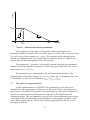
Flow
An arc in NETCELL must be connected to either zero, one or two incoming
arcs and zero, one or two outgoing arcs. The number of incoming arcs is used to
determine the type of the first cell in the arc. No incoming arcs indicates that the
upstream cell is an origin cell, one incoming arc
qm,k
Recieving Flow
Density
Sending Flow
k j,k
k 0,k
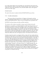
Figure 2: Generalized flow-density relationship
indicates that the first cell is an ordinary cell, while two incoming arcs indicate the
cell is a merge cell. Similarly, two outgoing arcs indicate that the last cell in the arc is
a diverge cell, one outgoing arc indicates an ordinary cell, and zero outgoing arcs
indicates a connection to a destination cell. This allows us to treat all the cell types
properly without actually storing the type as part of a cell.
An arc also stores information common to all its cells, e.g. the free flow speed,
capacity, jam density ..., which are, by default, the same for all cells in the arc. Thus,
6
if the user wishes to model an uninterrupted physical facility where some of the
conditions change (e.g. due to a lane drop or change in grade), (s)he may need to
split the original arc into two or more arcs.
Type 0 cell:
Ordinary cell
Type 1 cell:
Diverge cell
Type 2 cell:
Merge cell
Figure 3: Cell type specifications
Some of the above mentioned parameters may vary with time, e.g. If a
capacity-reducing incident takes place somewhere in an arc. Because this is of some
interest, this implementation of NETCELL allows variable capacities to be specified
at particular points in an arc, as if an incident had occurred. Although we shall refer
below to Òincident eventsÓ it should be understood that the procedure can also be
used for recurrent capacity reductions, such as metering of certain locations. Incident
events are discussed in the section below on the simulation event system.
Cells are stored as a linked list attached to the arc. They store traffic flow
information and occupancy only. Unless a cell has a cell specific set of flow
parameters because of an incident, there is no information about the physical facility
stored in the cell itself.
Where two arcs merge into a third, the simulation uses a merge priority
coefficient to determine the percentage of traffic allowed to enter the merge cell.
This value is stored in the downstream arc. The table of route choice coefficients
used to determine the percentage of traffic bound to a destination which takes each
leg of a diverge is stored in a similar way in the upstream arc. These values are used
only by the merge cell and the diverge cell, if any, of the arc. A considerable memory
savings results from storing them in the arc rather than in the cell itself, however.
7
Arc 1
Arc 0
Arc 0
Arc 2
Arc 2
Arc 1
diverge cell
merge cell
Figure 4: Merge and diverge cells in a junction
3.2
The traffic flow representation
In addition to the above input data, the simulation needs to be able to store
the state of the system at every clock tick. The state of the system consists of the
number of vehicles by destination and time of entry in every cell, nidt(t), the sum of
these over ÒdÓ, nit(t), and the cell occupancy, ni(t). The nidt(t) represent the number
of vehicles with destination d to have entered cell i in time interval [τ, τ+δ) that
remain there at time t; each such group of vehicles is called a ÒpacketÓ. The nit(t)
represent the number of remaining vehicles to have entered cell i in interval
[τ, τ+δ), irrespective of destination; each such group will be called a ÒcohortÓ. Packet
and cohort size information is necessary to maintain the first-in-first-out (FIFO)
discipline and to preserve the multicommodity nature of flow. A section below will
describe the algorithm for updating the state of the system. Here we describe how
the data are stored.
Instead of creating cell-specific tables with packet and cohort size information,
the program dynamically allocates storage for cohorts and packets to trace the
movement of traffic in the network. The dynamic allocation of these structures
eliminates the need for saving in each cell enough memory to store information
pertaining to the maximum number of packets that could possibly be present in it;
this is important because the maximum number of packets in a single cell could be
very high but at any given time t most cells in a network --- even a congested one --will be underutilized.
Each cell maintains a list of the cohorts which are currently in it. The cohort
stores the information about the vehicles in the network at the cohort level. A
8
cohort is an aggregate of the vehicles in its packets and stores only the total number
of all vehicles in the cohort, the cohort size, and the cell entry time (or more
specifically the lower end of the cell entry interval) and a pointer to its packets.
The packet list describes each cohortÕs component packets. It divides vehicles
inside a cohort into smaller units according to their destinations. A packet stores
only three items, its size, its destination and a pointer to the next packet in the
cohort. The order in which packets occur in the packet list for a cohort is not
significant. NETCELL maintains the FIFO order at the cohort level only. Traffic
bound for alternate destinations within a cohort are treated as uniformly distributed
within the cohort.
The linked list scheme allows vehicular progression to be traced easily and
efficiently. When a cohort moves from one cell to another without merging with
other cohorts, we only need to update the pointers in the cell cohort lists and the cell
entry time for that cohort. The cohort packet list can be left untouched. When
several cohorts enter a cell at the same time, they will merge into a single cohort. As
a result, a new cohort will be formed and the old cohorts and their packets will be
deleted.
To increase the speed of the simulation and to avoid excessive memory
fragmentation, the program maintains a list of free cohorts and free packets. When a
cohort is deleted, it is added to the free cohort list and its packets are added to the
free packet list. When a cohort is created, the program uses a cohort from the free
list. If either the free cohort list or the free packet list is empty, a block of additional
cohorts or packets is allocated. This minimizes the amount of memory
fragmentation in the program. Should NETCELL be unable to allocate additional
storage, the simulation terminates with an out of memory error.
Under the above representation, memory usage is bounded by the total
number of packets and cohorts existing in the network at any given moment. The
number of packets should be a few times smaller than the product of the total
number of destinations and the total number of cohorts existing in the network at
any given moment, because the typical cohort should only include packets for a
fraction of the destinations.
The movement of traffic from cell to cell is governed by the flow density
relationship for each cell. This relationship is defined by a set of parameters
associated with each arc.
By default the flow density relationship for an arc is assumed to be the
triangular flow density relationship shown in Figure 1. This is the model used in
reference [2]. It is also possible to use general forms of the flow density graph as
demonstrated theoretically in reference [4]. The general flow-density relationship
9
should then be described by two continuous, piecewise differentiable functions as
shown in Figure 2, one for sending flow and the other for receiving flow. The
actual flow entering a cell is determined by the minimum of the sending flow
computed from the occupancy of its upstream cell and the receiving flow computed
from the occupancy of the cell itself. This generalization has been implemented in
NETCELL in an approximation form.
Flow
To specify the sending and receiving flow curves for an arc, the user would
need to supply as input n points of data for flow and density as shown in Figure 5
where n = 6. The flow-density curve is then constructed by joining two neighboring
points with line segments. The resulting curve should be such that the absolute
value of the slope of each line segment is less than the free flow speed. An initial
point with coordinates (0,0) and a final point with coordinates (jam density, 0) are
assumed for the ends of the curve.
qm,k
k j,k Density
k 0,k
Figure 5: User-specified flow-density relationship
As the simulation runs traffic enters the system at origin cells and exits the
system at destination cells. The generation and destruction of traffic flows is
determined by a single, global, origin-destination (OD) table of OD flows. While, at
any given point of time, there is only one OD table, the table may change over the
course of the simulation. Time specific OD tables can be defined in the input file as
explained below.
3.3
Event representation
10
While NETCELL is primarily a clock based simulation model, it does contain
a mechanism to allow event driven changes to the state of the system. The program
maintains a list of events, each of which has an associated trigger time. Events are
processed at the start of the clock interval greater than or equal to the event trigger
time. Events are processed before any cell flows are calculated for that clock tick.
While the event system is a general mechanism, there are currently only four
event types defined. Two are trivial, the start simulation event and the stop
simulation event, while the other two change the state of network. These are the
incident event and the OD table update event.
The incident event changes the capacity of one cell. As the name implies, it is
intended to model accidents and similar occurrences though it can also be used to
model other events which affect capacity on a time basis, such as road work or even
signals. The OD table update event changes the global OD table used to generate
traffic by all cells in the network. The input file may contain multiple OD tables each
with an associated start time. When the system clock reaches the start time of an OD
table, that table replaces the previous OD table and the simulation continues. An OD
table remains in effect until the next OD table start time.
As mentioned above, the event system is a general mechanism for allowing
time dependent system changes. While the current implementation does not use
this feature extensively, it provides a easily expandable interface for future
enhancements. This might include such things as time dependent changes to the
route choice coefficients or time dependent flow-density relationships (e.g. due to
weather).
4
The Simulation Algorithm; Memory and Computational Time
Requirements
4.1
The simulation algorithm
Reference [2] proposed a cell transmission algorithm with two major steps: (1)
calculation of the inbound and outbound flows (by destination) for all cells, and (2)
revision of the cell occupancies (by time of entry and destination) as per the flows
calculated in step (1). When a cell is considered, its packet and cohort information,
along with the same information for its downstream neighbor(s), is updated based
on the flow between the two (or three) cells. The change in state due to the inflow is
realized automatically when its upstream neighbor(s) are considered.
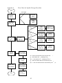
A flowchart of the whole program is shown in appendix 1. The program
initializes various structures and then reads the input file. After the input file has
been read, the program creates the arc and cell lists, the event list, and the OD table.
11
Then the program enters the simulation loop where it remains until an end
simulation event occurs. The simulation loop advances the clock and then
processes any events which have a time stamp less than or equal to the current clock
tick. After all events have been processed, the program updates the flows of each
cell.
The algorithm traces each arc in turn in the order in which they occurred in
the input file. Cells are considered in spatial order along an arc. The sequence in
which arcs and cells are considered is unimportant for the algorithm except in the
case of a cell directly upstream of a merge cell. In that particular case, the outflow of
the cell is calculated as part of the inflow calculation for the merge cell. In all other
cases the outflow of the cell and the inflow of the downstream cell or cells are
calculated together. There are five different procedures called to update cells,
depending on the connectivity of the parent arc and the cellÕs position in the arc.
They are updateOrigin(), updateDestination(), updateMerge(), updateStraight(), and
updateDiverge(). The flowchart in Appendix 1 shows the procedure which should
be invoked depending on the arc and the cell position in the cell list. Function
updateOrigin() calculates the inflow for a cell directly downstream from an origin
cell. Since an origin cell is an abstract entity and does not actually have a
representation in the arc and cell lists, this is a special case. Similarly,
updateDestination() is called for the last cell in arc which is directly upstream from a
destination cell.
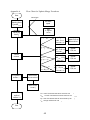
The three main procedures are illustrated by flowcharts in appendices 2,3, and
4. Function updateMerge() calculates the outflows of the two upstream cells and the
inflow and the outflow of the merge cell. Function updateStraight() calculates the
flow of an ordinary link (not part of a merge or diverge); i.e. the outflow of a cell and
the inflow of its downstream cell. Function updateDiverge() calculates the outflow
of the diverge cell and the inflows of the two downstream cells. The sequence in
which the cells and their update procedures are evaluated is as follows:
For each arc in turn:
Step 1: if the arc has no incoming arcs, call updateOrigin() for the first cell and move
to the next cell. If the arc has two incoming arcs, call updateMerge() for the first cell
and move to the next cell.
Step 2: if the current cell is not the last cell in the arc, call updateStraight() and move
to the next cell.
Step 3: if the arc has no outgoing arcs, call updateDestination() and move to the next
arc. If the arc has two outgoing arcs, call updateDiverge() and move to the next arc. If
the downstream cell is a merge cell, move to the next arc without processing this
cell, otherwise call updateStraight().
12
When the last cell has been processed, the overall occupancies ni(t) are
updated. The logic of the five update procedures called above are briefly described
below.
The updateStraight() and updateMerge() procedures are very similar
and can be described jointly. Let cell j be the downstream cell of the
current cell, i, with cell i+1 as the companion cell for merges. Using ni(t) and nj(t),
and n i+1(t) if the function called is updateMerge(), we first calculate the overall
flow(s) with the equations given in either section 2.2 or section 2.3 in Daganzo
(1994a). With these amounts as targets, which should be met to within a tolerance of
ε units, and using a FIFO discipline, the specific cohorts and packets to be moved are
identified and transferred. The tolerance level ε is needed to limit the fragmentation
of cohorts that can arise in certain instances; it should be a small number specified
by the user.
The updateDiverge() procedure uses as targets the maximum number of
vehicles that can be received by cells j and j+1, R j and R j+1, and the maximum
number of vehicles that can be sent by cell i, Si. These quantities are calculated with
the formulas in section 2.4 in Daganzo (1994a), with the old nj(t) , nj(t) and nj+1(t) as
inputs. The procedure then sends packets in FIFO order to the appropriate
downstream cell, split if necessary as per the route choice constants, bid. The process
is stopped when one of the three targets is met to within a tolerance of ε. The
flowchart includes more details.
Note that a packet will be divided in two parts (or three parts for diverges) if it
cannot exit a cell in its entirety. Conversely, two or more packets with the same
destination will become a single packet whenever they enter a cell in the same
interval; the buffers in the flowcharts achieve this. Note as well that our strategy
makes no attempt to preserve FIFO within packets and cohorts; only across packets
and cohorts. This introduces an error, but one which should be comparable with the
(small) length of a clock step.
4.2
Limitations, memory and computational time requirements
This section describes some of the size limitations on various parameters and
attempts to give some indication of the likely hardware requirements. This is
difficult due to the dynamic nature of the use of system resources and only an
approximate calculation can be done.
Many of the indices used in NETCELL are stored as integers. On most small
memory machines, such as desktop computers, this is a signed 16 bit quantity, so the
maximum allowable value of these indices is 32,767. In particular we note that a
13
network can have only 32,767 arcs. Each arc can have no more than 32,767 cells.
There can be 32,767 origins and 32,767 destinations in the network as a whole. These
are, however, limits which are unlikely to be a problem. Likewise, the number of
cohorts and packets is limited by the 32 bit pointers that form the linked list. This
number is so large that the maximum number of cells and cohorts is effectively
limited by the amount of available system memory.
The memory requirements are dominated by two major components, the size
of the network and the maximum number of cohorts in the system at any given
time. The former is determined at the initialization stage of a simulation run. The
latter is dynamic, varying with system evolution as the simulation progresses.
Almost all of the memory to store the network geometry is used to store the
arcs and the cells. Let A be the total number of arcs in the network. The memory to
store the arcs is 166 + 8D where D is the number of destinations in the network. If M
is the average number of cells per arc, there are MA cells in the system which
require 40MA bytes of storage. So the total memory required to store the network
geometry is on the order of (40M + 166 + 8D)A.
The total number of cohorts existing in the network can be estimated from
the average cell delay in the system. Let average cell delay at clock tick t be d(t), d(t) =
(1/MA) Σi d(t). Let T = maxt{d(t)}. The total number of cohorts required is on the
order of MAT. The size of the packet list for a cohort is destination dependent. In the
worst case where we assume that each cohort is mixed with components heading for
every destination, the size of each cohort is (24+10D) bytes. The total memory
required for cohorts are MAT(24+10D) bytes. The total memory requirement for the
simulation is on the order of 10MATD bytes. As an example, if we have a network
with 1,000 arcs and an average of 15 cells per arc, a maximum average delay of 2
clock ticks and a network with 50 destinations, the memory to store the network
geometry is approximately 1.2 megabytes and the memory to store the cohorts and
packets is approximately 16 megabytes. A total memory requirement of 18 megabytes
is well within reason for many desktop computers and low end workstations.
The computational time requirement for a simulation run in the worst case
is on the order of SMADd where S is the simulation length in number of clock ticks,
and d is the average cell delay, d = (1/SMA) Σi Σt di(t) in clock ticks.
There are non-trivial disk storage requirements for output files as well. The
section below on output files has detailed descriptions of the various output options
available. The most detailed file, the cell occupancy file, has a storage requirement of
5MA per clock tick. In the example above this is 75,000 bytes per clock tick. If the
simulation covered an 8 hour period with a 5 second clock, the output file would
occupy 432 megabytes. A 2 hour simulation would require 108 megabytes.
14
5
File Structure; Input and Output Processes
The input and output files are related via DOS derived file extensions. The
are potentially four files used by NETCELL, characterized by four different
extensions. The .INP file is the input file for the simulation run. Two output files
are always produced, the arc flow file which has a .FLW extension, and the arc travel
time file, which has a .OUT extension. A file containing cell occupancies can be
produced if that option is selected in the input file. The cell occupancy file has a
.TRC extension. All filenames are based on the input file name, differing only in the
extension.
5.1
The input file: .INP
All input data is contained in a single text file whose name can be chosen by
the user but whose extension must be .INP. The input file consists of five sections
containing data defining the simulation parameters. These sections are described in
detail below and a sample input file is provided in appendix 5.
There are six sections to the input file: the control parameters, the geometry
information, the curve specifications, the routing information, the OD table
specifications, and the incident information. The sections must occur in that order
and are separated by a keyword marking the end of the section. Sections may be
empty but the appropriate keywords must still appear. Within each section, input
lines start with a type keyword followed by a variable number of parameters on a
single line. Parameters are separated with one or more spaces or tabs. With the
exception of the OD tables, order of lines within a section is unimportant. Keywords
are always in all capital letters Any line not starting with a recognized keyword is
treated as a comment line and ignored. In general, if the same parameter is multiply
defined, the last definition applies and earlier definitions are discarded. After the six
sections, the input file may have a single line with the keyword ENDINPUT. This
tells NETCELL to stop processing the input file. The ENDINPUT line may be
followed by additional comment lines which are not read at all.
5.1.1
Simulation controls
This section defines the overall simulation parameters. It must be the first
section in the input file and it ends with the keyword: ENDCONTROLS. The order
of lines is not significant. Possible parameter lines are:
TIME b e
This line specifies the beginning and end times (b and e) of the simulation run. It is
15
anticipated that these times specify seconds or hours based on a 24 hour clock with 0
as midnight but this need not be the case. It is important to note that all times
throughout the input file are in the same units. Thus, if the beginning and end
times are in seconds, the clock tick, arc speeds, arc capacities and origin-destination
flows must all also use seconds.
The memory usage of NETCELL is independent of simulation length. A long
simulation period specified here will not result in running out of run-time memory
but it will generate big output files.
UNITS
Seconds
This line is optional and specifies the unit of time that the user has chosen. The
information is used for labelling the time axis when displaying flow curves in
NETVIEW. It is not used in any way in the simulation itself.
CLOCK
d
This line specifies the discrete time interval between clock ticks in the time units
chosen by the user. It may be whole or real valued. This value in conjunction with
the arc lengths and speeds determines the number of cells in an arc. The size of this
value has a major impact on the memory usage of the simulation. There is no
default value.
EPSILON
e
In NETCELL vehicle quantities are real-valued. In certain cases, the size of a cohort
can be very tiny with a size of, for instance, 0.0001. At any clock tick, if the size of a
cohort residing in a cell falls below this user-specified threshold, the cohort will not
be transferred alone at the current time. Instead, it will wait till some future time to
be transferred together with other cohorts. This is a real number and if the line is
omitted, the default value is .0001.
OUPUTOCC b
This line controls the production of the cell occupancy file. The parameter b can be
either 0 or 1. A value of 1 will cause NETCELL to write the cell occupancies for each
clock tick to the .TRC file. See the section below for more information about this
output file. This line is optional and the default value is 0.
ENDCONTROLS
This ends the simulation control parameters section and must be the last line in the
section.
16
5.1.2
Road geometry
The data in this section specifies the geometry of the network. It ends with the
ENDGEOMETRY keyword. Valid lines are:
NODE nodenum type x y
Information about the nodes is used to set up the connections between arcs. After
the arc list is constructed, the node information is discarded before the simulation
begins. The nodenum parameter must be ±32,767 and must be an integer. The type
parameter can be 0,1 or 2. A type 0 indicates an ordinary node, type 1 indicates an
origin node, and type 2 indicates a destination node. The values x, y are 16 bit
integers (|x|, |y| ≤ 32,767) denoting the location of the node in a rectangular
coordinate system. They are used by the NETVIEW program for drawing a
representation of the network. These values must be present but need not have any
real meaning. For instance, all nodes may be located at point 0,0 without causing any
problems for either NETCELL or NETVIEW.
ARC arcnum upNode downNode length speed capacity jamDensity
The input of roadway geometry is arc-oriented. Here each line contains the
information about a single arc. There are a total of 7 columns in the data entry. The
first three columns of this data entry define the network connectivity with arcs and
nodes in a conventional way. The arc number must be an integer and is used in
many of the input parameter lines described below. The upstream and downstream
node parameters are valid nodenumbers from a NODE parameter line. The NODE
line need not appear before an ARC line which references it, references are resolved
after all the lines have been read and processed. The program generates an error if
an ARC line contains a reference to a node which is never defined before the end of
the geometry section.
The fourth and fifth columns specify the length and free flow speed of the arc. The
length and speed of the arc are given in the same units of measurement for time
and distance used elsewhere in the input file. Both are real numbers. We recall that
the actual arc length used by the computer algorithm is the integer multiple of cell
length (clock tick interval times the flow speed) that is closest to the specified value.
Thus, short clock intervals result in a more accurate representation of the network.
NETCELL requires each arc to be represented by at least two cells. This requirement
can be met by shortening the clock interval.
The last two columns, are used to specify capacity and jamDensity. The arc input is
sufficient to define a triangular flow-density relationship of the form discussed in
17
section 3.2. The capacity is assumed to be in vehicles/(unit distance). The
jamDensity is in vehicles/(unit distance).
ENDGEOMETRY
This section must end with a line starting with ENDGEOMETRY.
5.1.3
Curve specifications
This section defines any custom flow density relationships for the arcs in the
network. It ends with the ENDCURVE keyword. There is only one possible input
line, the QDCURVE parameter line, which can have two variants. This section may
be empty except for the ENDCURVE line.
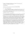
QKCURVE arcNumber 1 waveCoefficient
The second parameter in a QKCURVE input line is a type code specifying what kind
of a curve is being defined for the arc specified by the arc number. A type code of 1
indicates that the curve for this arc is a trapezoid such as those of Figure 6. When
this option is used the information in the ARC definition line is still used to specify
the parameters qm,k, vf,k and kj,k of Figure 6, so that only the slope of the trapezoidÕs
right side remains to be determined. This is done by means of the waveCoefficient
parameter, α, which gives the absolute value of said slope in units of vf,k. This
absolute value cannot be less than the default; see Figure 6. In addition, since the
backward moving wave speed cannot exceed the free flow speed, the upper bound of
the wave coefficient must be 1. (It is in reality serveral times smaller than 1.) The
lower bound of this parameter is determined by the values of the free flow speed,
jam density, and maximum flow as specified in the ARC definition line. For
example, suppose an arc has a jam density = 180 vpm, free flow speed = 60 mph, and
maximum flow = 1800 vph. The lower bound of the wave coefficient is 0.2. The
choice of the wave coefficient, ranging from 0.2 to 1 in this case, gives different
shapes of the flow-density relationship as shown in Figure 6.
18
Flow
qm,k
α def
α max =1.0
-w k =α v f,k
V f,k
k j,k
k 0,k
Density
Figure 6: Trapezoidal q-k curves with wave speed
greater than the default value
QKCURVE arcNumber 2 points x1 y1 x2 y2 x3 y3 ...
This form of the QKCURVE parameter line forces NETCELL to use a piece-wise
linear flow-density curve specified by the user for the given arc. The curve is
specified by the provision of an arbitrary number of xy coordinate pairs denoting
points along the desired curve in the same units used for the arc definition. The
points parameter in the above line indicates how many coordinate pairs follow on
the input line. The number of pairs must match the points parameter. All the
values should be non-negative real numbers and the x-values should be smaller
than the jam density for the arc. The x sequence must be strictly increasing while
the y sequnce should be unimodal (no multiple maxima.) An initial point at (0,0)
and a final point at (jam density, 0) are added by the program. The pairs produce a
line segment graph of the type shown in Figure 2 starting at the origin and ending at
the jam density. The information provided with this option overides the capacity
provided for the arc in the geometry section. The maximum slope of the linear
segments (in absolute value) cannot exceed the free flow speed specified for the arc
in the geometry section.
ENDCURVE
This section ends with the ENDCURVE keyword.
5.1.4
Routing information
19
This section specifies the behavior of the traffic flow at merge and diverge
junctions. It ends with the ENDROUTING keyword. There are two possible
parameter lines as follows:
DIVERGE fromArcNumber toArcNumber c1 c2 c3 ... cD
The route choice coefficients, cd, denote the proportion of traffic flow heading for
destination d that chooses one particular downstream leg of the diverge junction.
The arc number of this leg is identified as the ÒtoArcNumberÓ parameter. In the
current implementation, the coefficients are time and situation invariant. A later
version may enhance the modelling of diverge junctions to dynamically adapt these
values based on either state information, such as congestion levels, or time. The
ÒfromArcNumberÓ is the number of the arc ending at the diverge; it is used to
identify the diverge junction to which this parameter line applies. Only one set of
coefficients is required for each diverge junction as, by definition, the coefficient for
traffic flow taking the second arc is 1 - the coefficient of the first arc. For example, for
a diverge junction which is a part of a network with two destinations, an input line
would look like:
DIVERGE 0 1 0.8 0.3
This would specify that at the diverge cell at the end of arc 0, 80% of the traffic flows
going to destination 1 and 30% of the flows going to destination 2 would choose the
diverge branch represented by arc 1. The parameter line is expected to have as many
coefficient entries as there are destinations in the network. The order of coefficients
corresponds to the order in which destination nodes appear in the network
geometry section of the input file. If there are less coefficients in the line than
destination nodes, an error message will be printed and the program will terminate
after all input lines have been read. An error message is also produced if the set of
coefficients is chosen erroneously such as to cause some flow to be routed to the
wrong destination.
MERGE fromArcNumber toArcNumber coefficient
The merge coefficient denotes the fraction of vehicles which come from
each approach in a merge junction when the supply of vehicles from
each approach is not exhausted. This entry is similar to that of route choice
coefficients and is time-invariant as well. The user only needs to specify the
coefficient with respect to one of the arcs upstream of the merge node. The program
will then identify its companion arc and assign the remaining fraction to that arc.
The default for all coefficients is 0.5. A warning message will be printed for merge
junctions left with the default but the simulation will continue to run.
20
ENDROUTING
The ENDROUTING keyword ends the specification of route choice and merge
coefficients.
5.1.5
OD table specification
This section specifies the generation of traffic flows in the simulation. Traffic
demand is represented as a two dimensional matrix with origin as the first
dimension and destination as the second. This is the only section in which the order
of lines within a section is significant. The two dimensional tables are input as a
series of lines, one for each origin, with each line specifying the traffic from that
origin to all destinations in the system. Multiple OD tables may be specified for a
single simulation run. Each table has a starting time which NETCELL uses to update
the OD table in use at any particular time step within the simulation. The starting
time for a table is specified in a parameter line which must appear before the origindestination lines to which it applies. Thus, the format for an OD table is a ODTIME
line specifying the starting time for the table, followed by one ODROW line for each
origin, with each line containing demand values for each destination. The format of
the lines is:
ODTIME time
This sets a start time for a new OD table. The time does not have to be within the
simulation start and end times but must be in the same units. There is an implicit
ODTIME 0 line at the beginning of the OD table specification section. This allows the
user to specify an OD table which will be used from the beginning of the simulation
until such time as another OD table start time has been reached.
ODROW origin dest1 dest2 ... destD
The ODROW line sets the traffic demands from the specified origin to each of the
destinations in the network. The time unit should be the same as that used to define
ÒcapacityÓ and Òtime.Ó As for the route choice coefficients, the order of demands is
assumed to correspond to the order in which destination nodes occur in the
geometry section of the input file. Similarly, if there are not as many parameters are
there are destinations an error message is displayed. There should be the same
number of ODROW lines following an ODTIME line as there are origins in the
network, but this is not required. The order of the lines within a table is not
significant as the origin parameter is used to determine which line in the OD matrix
is being defined. Nor do the lines need to be directly sequential. There may be one or
more comment lines between ODROW lines. If no line for a particular origin
appears in the table entry, that row of the OD matrix is set to zero. If multiple lines
21
for a single origin appear in the same table entry, the demands in the last line are
kept and previous values are discarded. Warning messages will be printed for lines
with fewer values than destinations, lines left with default values, and repeated
lines for the same origin.
ENDODTABLES
The end of this section is marked with the ENDODTABLES keyword line.
5.1.6
Incident information
This section allows the specification of changes to the capacity and jam
density of particular locations along an arc at arbitrary times. The section ends with
the keyword ENDINCIDENTS. There is only one possible kind of parameter line:
INCIDENT arcNum distance startTime endTime maxFlow
The location of the incident is specified as lying a specific distance along the
indicated arc. For instance, an incident might lie .5 miles from the start of arc 1. If
the distance specified is longer than the length of the arc, the incident is ignored.
The distance along the arc is used to determine which cell contains the incident. The
new capacity value will apply to that cell alone. The start and end times set the
period within which the changed capacity is valid. They are in the same simulation
time units as all other time parameters. The maxFlow parameter is the new value
for the cell capacity. This value replaces the default value the cell normally uses.
When the incident ends, the cellÕs capacity returns to the default value for the arc.
Incidents cannot be nested or overlapped within a single cell. If an incident affects a
particular cell from time 10 to time 40 and a nearby second incident affects the same
cell from time 20 to time 30, the cell will use the value from incident 1 from time 10
to 20, the value from incident 2 from time 20 to 30 and the default arc value from
time 30 on. The remaining period for incident 1 is lost. Because this may or may not
be done intentionally, the program issues a warning every time it happens. The
problem should not arise if the cell length is smaller than the physical separation
between the incidents; thus, it may be removed by decreasing the clock step. To
model multiple ÒincidentsÓ at the same location, e.g. variable metering rates, the
input file should specify a sequence of non-overlapping incidents at the same
location. An incident does not affect the free flow speed for the affected cell. (This
should not be a cause for errors if the cells are small, as required by the theory
underlying NETCELL.) The geometric form of the flow density relationship for the
cell with the incident will be identical in shape to the one chosen for the original,
except that it is truncated at the top.
22
ENDINCIDENTS
This section ends with the ENDINCIDENTS keyword. The incident section is the
last section of the input file and no further lines will be processed.
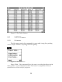
5.2
Outputs
A set of two, and optionally three, output files will be generated by NETCELL
when it runs. All three output files are text files with a simple column based format
which can be easily imported into software packages such as LOTUS, QPRO, or Splus
to make various plots. The three files are the arc cumulative count file, the arc
travel time file, and the cell occupancy file. The names of the output files are all
based on the input file name with different extensions for each file type. The acr
count file has the extension .FLW, the cell occupancy file has the extension .OCC
and the arc travel time file has the extension .OUT.
The arc cumulative count file is named similarly to the input file but with a
.FLW extension. This file is used as the input file for NETCELLÕs companion
postprocessor program, NETVIEW. As such its format is slightly more complicated
than the other two output files. The arc count file starts with a duplication of the
input file. All lines are echoed from the input file to the arc count file as these are
processed, including all comment lines. This allows the program NETVIEW to read
the arc count file alone and reconstruct the network and simulation parameters.
Including the comment lines allows the user to easily rerun the simulation using
the arc count file as a new input file. The input section of the arc count file ends
with an ENDINPUT keyword line. This line is added if there was no such line in the
original input file.
The remainder of the arc count file contains one line per clock tick of arc
inflow and outflow counts. The output line contains values for every arc in the
network for the clock period. There are four values per arc, the inflow to the arc for
the clock interval, the outflow from the arc for the clock interval, the cumulative
inflow to the arc and the cumulative outflow from the arc. The values show one
decimal place and are separated by spaces.
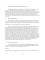
23
Cumulative counts
T i (t)
h
t
Time vehicle h
enters cell i
di (t)
Time
Time vehicle h
exits cell i
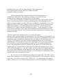
Figure 7: The computation of cell travel time T
i (t)
The arc count file is used at the end of the simulation run to produce the
second output file, the arc travel time file. The arc travel time file stores the travel
times for each arc, Ti(t) where Ti(t) is the time it takes to traverse arc i when the arc
was entered at time t. Under FIFO, the time at which a vehicle will exit an arc
entered at time t is the time di(t) at which the cumulative number of departures
from the arc equals the sum of the initial arc occupancy and the cumulative count of
arrivals to the arc in [0,t). Thus, Ti(t) = di(t) - t. See Figure 7. This calculation applies
to travel times for individual cells as well. The only difference in the treatment of
cells and arcs is the placement of the counting locations; see Figure 8. The Ti(t)'s can
be used off-line to reconstruct route travel times and calculate time-dependent
shortest paths. The travel times are stored as one line per clock tick with the start of
the time interval at the beginning of the line followed by one value per arc. Values
are separated by spaces.
Production of the third output file, the cell occupancy file, is determined by
the flag on the OUTPUTOCC line of the input file. This line is optional and by
default it is not produced as it can grow to very large size on even moderate sized
problems. The cell occupancy is output as a single line per clock tick with all the
24
current occupancy values for all the cells in the network on that
arc
arc
arrival
counts
cell
arrival
counts
cell
departure
counts
arc
departure
counts
Figure 8: Locations to take cumulative counts
one line. Cells appear in the output line in the order in which the arc to which they
belong appeared in the input file. Within the arc, cells are in sequential spatial order
(upstream first.) There is no indication of the breaks between cells belonging to one
arc and the cells belonging to the next. Thus, to use this file to do further analysis,
while possible, may require some effort to reconstruct the arc to cell translations.
6
An Example Network
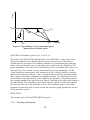
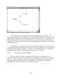
The example given in this section is a simple network with a
single origin, two destinations and a single diverge junction. It
is based on the sample .INP file given in appendix 5. As shown in
Figure 9, the upstream section is represented by a single arc, and
each of the diverge branches by two arcs in series. We assume that q-k
relation depicted in Figure 10 holds for all links and 50% of the
traffic goes to each destination. Initially, the upstream link is
assumed to be operating at capacity when a temporary incident
0
Origin
0
1
2
3
4
Destination 1
5
Destination 2
1
2
3
4
Figure 9: Roadway geometry for the example
25
partially blocks one of the diverge branches. The incident lasts
for a certain period of time until it is cleared and traffic
gradually returns to normal.
Node 0 represents the origin and nodes 4 and 5 represent the two
destinations, respectively. The roadway geometry is governed by four
parameters, the capacity (qk), density (kj,k), free flow speed
(vf,k), and a wave coefficient α which is universal for all arcs. The capacity for each
arc is .8 vps, the jam density 144 vpm, and the free-flow travelling speed .01667
miles/sec (approximately 60 mph). The wave coefficient is calculated to be 0.5. The
length of a clock tick for this example is set to be 5 seconds. It is also shown in the
input data set there is an incident taking place inside arc 1. The location of the
incident is 0.375 miles from the upstream end of arc 1. Traffic demands at origins,
route choice coefficients, and some other simulation control parameters are also
given in this input data file. We also specify that the output file for occupancy data
should be created.
The first step in the simulation run is to convert the input
data into their corresponding cell representation. For the purpose of illustration, we
will discuss further the result of the conversion. The first two parameter lines in the
simulation control parameters determine the total steps of the simulation run, i.e.
(1250-0)/5= 250 steps or clock ticks. Under cell representation, arcs 1 to 4 will be
represented by 15 cells and arc 0 by 30 cells. The length of each cell can be calculated
as 1/12 miles, as well as the maximum occupancy (N=12), and maximum flow
(Q=4). The prespecified incident is identified to be inside cell 55 (one of the cells
representing arc 1) which lasts for 100 clock ticks. When the incident occurs, Q for
cell 55 will be dropped to 1. The total number of cells used for this simple network is
93. For the traffic demands, or the departure rates, there are four vehicles leaving
the origin zone at every clock step. Of these, two are heading for destination node 4
and the other two for destination node 5.
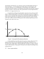
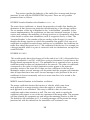
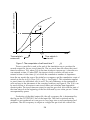
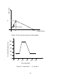
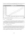
We can now run the simulation and specify the input file ÒTEST.INPÓ when
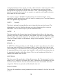
asked. The simulation run covers a period of 1250 seconds, or 250 clock ticks. The arc
travel time over time is stored in file ÒTEST.OUTÓ. As an illustration, the time it
takes to traverse arc 1 for vehicles entering the arc at time t is displayed in Figure 11.
26
Flow (vps)
.8
v=.01667 mi/sec
144
48
Density (vpm)
Figure 10: q-k curve for every arc in the example
Arc travel time (seconds)
250
200
150
100
50
0
0
50
100
150
200
250
Time (seconds)
Figure 11: Travel time T
27
i (t) for arc 1
7
Introduction to NETVIEW
The NETCELL simulation package consist of two programs, NETCELL, the
simulation model itself, and NETVIEW, a postprocessor for viewing an output file
from NETCELL. NETVIEW takes as input the .FLW output file from NETCELL and
allows the user to examine the cumulative flow-time curves, and the simulation
occupancy counts for any selection of network arcs. Curves and tables may be
printed and the simulation data, or a subset, may be saved in a format compatible
with spreadsheets or statistical analysis packages for further analysis.
NETVIEW is a graphical windowing program and is available for two
platforms, the Apple Macintosh, and Microsoft Windows.
8
Installing the NETCELL simulation package
Installation of the NETCELL simulation package is very simple. There are
only two files, one for each executable. There is no installer program as installation
is straightforward enough not to warrant one.
8.1
Installation on the macintosh
Insert the NETCELL distribution disk into the floppy drive. On the hard disk,
create a folder called ÔNETCELLÕ or something similar. This can be in a nested folder,
if desired. Drag all the files from the floppy to the new NETCELL folder. The
NETCELL simulation package has been tested on both 68k macintosh systems and
on powerMac systems running system 7.x. It may run on system 6 machines but this
has not been tested. Both programs are Ôfat binariesÕ and run in native mode on both
680x0 and powerPC systems.
The default memory partition is set to 1 megabyte, but this may not be
suitable for the simulation runs any particular user may want to do. The memory
use of NETCELL is highly dependent on the number of cells and the number of
cohorts in the simulation and is difficult to predict apriori. If running NETCELL
produces any out of memory error messages, increase the memory partition and
retry the simulation. To increase the memory on either program, select the program
icon, ÔNETCELLÕ or ÒNETVIEWÕ, and select the item ÔGet InfoÕ from the File menu
of the finder. Increase the amount of memory allocated to the program in the
preferred size box to some larger number.
8.2
Installation under windows
Insert the NETCELL distribution disk into the floppy drive. Either at the DOS
prompt or using the Windows file manager, create a subdirectory called ÔNETCELLÕ
28
or something similar. This can be in a nested subdirectory, if desired. Copy the file
ÔNETZIP.EXEÕ from the floppy to the new NETCELL directory. This file is a self
extracting archive file. At the DOS prompt type ÔNETZIPÕ. This should expand the
file and create all the files in the NETCELL simulation package. Once the file has
been expanded, the NETZIP.EXE file may be deleted. The NETCELL simulation
package has been tested under windows for workgroups 3.11. It may run under
windows95 or under windows NT but no testing has been done. It should work
under windows 3.1 as well. The NETCELL program comes in two versions, one for
DOS and one for windows. The DOS program ÔNETCELLD.EXEÕ uses normal DOS
memory only and so is limited to problems which can run under the 640k memory
limitation of DOS. The windows version ÔNETCELL.EXEÕ uses whatever windows
resources are available to it so it can potentially simulate much larger networks.
Once the programs have been copied to the hard disk, the user should create
windows program icons for them. Under the windows program manager, create a
new program group called ÔNETCELL simulation packageÕ. It can be saved in the
NETCELL directory or in the windows directory. In the new program group, create a
program icon for the NETCELL simulation executable. To do this, select ÔNewÕ
under the file menu of the program manager and click on Ôprogram iconÕ in the
resultant dialog box. Name the new program icon ÔNETCELLÕ. Enter the full path
and program name for the NETCELL program and click the OK button. The path to
enter should be ÔC:\NETCELL\NETCELL.EXEÕ. Select the program icon and select
ÔPropertiesÕ under the file menu. Under working directory, enter the path for the
NETCELL directory. This will typically be ÔC:\NETCELLÕ. This will set NETCELL to
store its output and working files in the NETCELL directory when run.
Next, create a program icon for the NETVIEW program in the same way. The
path and program name should be ÒC:\NETCELL\NETVIEW.EXEÓ. The working
directory for NETVIEW may be set to the NETCELL directory as well, though this is
not required. At this point the NETCELL simulation package is installed and ready
to run.
The memory use of NETCELL is highly dependent on the number of cells and
the number of cohorts in the simulation and is difficult to predict apriori. If running
NETCELL produces any out of memory error messages, the user may have to
decrease the system resources used by other things. This may involve quiting any
background programs, or in more extreme cases removing device drivers or other
memory resident programs and rebooting the machine.
9
Running NETCELL
Once the programs have been installed, the NETCELL simulation program is
ready to be run. Before running NETCELL, the user must create an input file. The
29
input file can be created in any word processor or text editor. If using a word
processor, the file must be saved as a text file, which usually requires using a special
technique when saving the file. Consult the userÕs manual for the specific word
processor for information on how to do this. Most word processor wrap long lines to
within the document margins. Some of the lines in a NETCELL input file may be
very long. Any long lines must be on a single line and not wrapped. Saving as text
will usually not wrap lines, although an option, usually called something like
Òconvert soft returns to hard returnsÓ will result in breaking long lines in the text
file. This will generate input errors when the file is read by NETCELL.
The input file is described in detail in section 5.1 above. That section describes
how the file must be laid out and what the available input parameters are. A sample
file is shown in appendix 5 as well.
Once an input file has been created, the user is ready to run the NETCELL
simulation program. The input file should be copied to the NETCELL directory
(folder) before running NETCELL. As discussed in section 5, the name of the file
must end in the extension .INP.
To run NETCELL, under windows or macintosh, double click on the
NETCELL program icon, under DOS, type ÔNETCELLÕ. This will start the simulation
program. NETCELL will prompt the user for the name of the input file and wait for
the data to be entered and the return key to be pressed. The user should enter just
the initial portion of the name without the .INP extension which is assumed. If the
file cannot be found by NETCELL, the program will terminate with an error
message. IF the file is found, the program will read it and start the simulation.
Errors in the syntax of the lines of the input file will cause the NETCELL program to
terminate with a message indicating what the nature of the problem is. If an input
file is failing to read properly, the lines should be carefully checked to be sure that all
lines have the correct number and type of parameters. Also check that all input lines
start with a keyword and that the keyword is in all capital letters. Lower case
keywords are treated as comments and ignored.
As the program runs it prints the current clock at each step of the simulation
to the screen. This is informational only, to let the user know where the program is
in its execution and allow an estimate as to the completion time. A run completed
message is printed on the screen when the program terminates. At this point,
NETCELL has produced an output file with a .FLW extension which can be viewed
with the NETVIEW viewer application.
10
Running NETVIEW
To run the NETVIEW program, double click on the NETVIEW program icon.
30
NETVIEW is a viewer of NETCELL output files only, it is not an input processor in
any way. NETCELL produces three output files, the arc cumulative flow file, the arc
travel time file, and the cell occupancy file. The NETVIEW program uses the arc
cumulative flow file, which always has a file extension of .FLW, as its input. See
section 5.2 for detailed information about the format of the arc cumulative flow file
and about the other NETCELL output files.
When NETVIEW starts, it presents a standard file open dialog box. The user
must have already run NETCELL and have an arc flow file available. When the
open dialog appears, select the .FLW output file and click on the OK button.
NETVIEW will attempt to open and read the selected file. If the selected file is not a
valid input file, the program will display an error alert. If this happens, most
functions within NETVIEW will be unavailable and the display windows will be
empty. Select open from the file menu and reselect a valid NETCELL arc cumulative
flow file.
After the arc flow file has been read, the user can generate flow-time curves
for the arcs in the network, print graphs or tables and export the data to other files.
To work with another input file, simply select ÔopenÕ from the file and select a
different arc flow file. Only one file can be open at a time, so opening a second file
will close the first automatically.
10.1
NETVIEW display windows
The NETVIEW program presents the user with four display windows and
four menus to manipulate them. The windows are the network window, which
displays a graphical representation of the network, the arc selection window, which
allows the user to select and deselect the arcs which are used to calculate results, the
curve window, which displays the flow-time curves for the selected arcs, and the
table window, which displays the cumulative counts and other information for the
selected arcs.
10.1.1
The network window
The network window shows a graphical representation of the input network.
Nodes are shown as small circles, with connecting arcs drawn with black lines. Arcs
are labeled approximately in the center of the arc with the arc number. The graphical
layout depends on the x,y coordinates of the nodes in the NETCELL input file, as
described in section 3.1. Since these coordinates are not necessary to run the
NETCELL simulation, the network representation may not correspond to the actual
network.
31
Figure 12: The Network Window
The network is initially scaled to fit in the default network window. The
window is resizable and scrollable and the network can be enlarged or reduced. The
Option menu contains two commands, ÔZoom InÕ and ÔZoom OutÕ. Zoom In scales
the network up by a factor of two, while Zoom Out reduces the network size by a
factor of two. If the network nodes do not have reasonable coordinates, this window
may appear blank.
The network window provides a view of the network only. It is provided as
an aid to the user in selecting arcs of interest to examine. When the arc selection list
is updated (the user picks ÒApplyÓ or ÒDoneÓ in the selection window as described
below) the selected arcs will be displayed in red on color monitors.
10.1.2
The arc selection window
The arc selection window is where most of the user interaction in the
NETCELL Viewer takes place. On the left is a scrolling list of selected arcs. Initially,
this list is empty. Using the number entry field and the buttons on the right, the
user adds and removes arcs from the selection list. The selection list, in turn,
determines the contents of the curve and table windows.
32
Figure 13: The Arc Selection Window
To add an arc to the selection list, the user enters the arc number in the arc
number entry field in the top right of the arc selection window, and clicks on the
ÔAddÕ button. If the arc number entered is valid, the arc will be added to the selection
list and the list on the left will update. Arcs appear in the list in the same order as
they appear in the input file.
To remove an arc, the user enters its number in the entry field and clicks the
ÔRemoveÕ button. If the arc was selected, it is removed from the list. The ÔAdd allÕ
button selects all arcs in the network while the ÔClear AllÕ button deselects all
currently selected arcs.
The network, curve and table windows are updated only when the user
indicates they are done adding and removing arcs from the selection list. This is
done in one of two ways. Clicking on the ÔDoneÕ button, or pressing the return key,
will update the arc selections and close the arc selection window. The curve and
table windows will update to reflect the new arc selections. If the user would like to
see the updated curves and table, they can click on the ÔApplyÕ button. This updates
the arc selections and the other windows but keeps the arc selection window in front
to allow the user to make further changes to the arc selection list. The ÔcancelÕ button
33
closes the arc selection window without updating the arc selection list. The selection
list will revert back to the list in effect after the last apply or done command.
Figure 14: The Curve Window
10.1.3
The curve window
The curve window draws the inflow and outflow flow-time curves for the
combined selected arcs. This shows the combined flow counts versus time for all the
arcs selected. Figure 7 shows a flow-time curve for the example input file and
section 5.2 discusses the relationship between the flow-time curve and the arc travel
time. The window is resizeable and printable.
10.1.4
The table window
The table window shows the detailed data for the combined selected arcs. For
each time slice of the simulation, the table shows the inflows and outflows for the
arcs for that time slice and the cumulative inflows and outflows. The values shown
are the sum of the inflows and outflows for the arcs in the arc selection list. This
window is also resizeable and printable. The data in it can also be exported in a
format compatible with most spreadsheets to allow further data analysis.
34
Figure 15: The Table Window
10.2
NETVIEW menus
10.2.1
File menu
The file menu contains the commands for open and closing files, printing
various output windows, exporting data and quitting.
Figure 16: The File Menu
Export Table - This command allows the user to save the data shown in the
Table window as a tab delimited text file. This format is compatible with most
spreadsheets and data analysis programs.
35
Page Setup - This command allows the user to set various printing
parameters.
Print Curves - This command prints the vehicle arrival and departure curves
for the selected arcs. The graph is scaled to fill a page.
Print Table - This command prints the data in the Table window.
10.2.2
Edit menu
The edit menu is the standard edit menu for the macintosh or for windows.
The only window in which edit commands are functional is the arc selection
window. In that window, the value in the data entry field for the arc number may be
copied, cut or pasted. None of the other windows have any editable data in them to
which the commands of the edit menu can be applied.
Figure 17: The Edit Menu
10.2.3
Options menu
The two options in the ÔOptionsÕ menu apply to the network window only.
They allow the user to change the scale with which the network is drawn. The
Zoom In command enlarges the network view by a factor of two while the Zoom
Out command shrinks the network view by a factor of two. Either command can be
repeated to enlarge or reduce the view further. When enlarging the view, there may
be no portion of the network visible In the window. To see the network, use the
scroll bars to move around the window and locate the network.
36
Figure 18: The Options Menu
10.2.4
Windows menu
The windows menu allows the user to manipulate the display of the various
NETVIEW windows. Selecting any of the show commands brings that window to
the front, making it visible if necessary. The windows can be rearranged or closed
using the title bar and close box or close menu in the top left corner of the title bar if
desired. They can be redisplayed and brought to the front using the windows menu
Figure 19: The Windows Menu
37
References
[1] DAGANZO, C.F. (1994) ÒThe cell-transmission model:
A dynamic representation of highway traffic consistent with the
hydrodynamic theoryÓ. Trans. Res. B, 28 (3), (in press).
[2] DAGANZO, C.F. (1994a) ÒThe cell transmission model: Network
trafficÓ. Trans. Res. B (accepted).
[3] LIN, WEI-HUA & C.F. DAGANZO (1994) ÒTechnical Description of NETCELL:
General Framework and Data StructureÓ.
[4] DAGANZO, C.F. (1995) ÒA Finite Difference Approximation of the Kinematic
ModelÓ. Trans. Res. B. Vol. 29B, No. 4, pp. 261--276.
38
Appendix 1:
Flow Chart for NETCELL
Start
Open files
Read
input
Event type
Incident
change
Setup arcs,
cells, events
Initialize
OD table
change
Process
events
Cell type
Update
origin
Update
first cell
Simulate
Update
merge
Update
cell
occupancy
Travel time
calculation
Update
straight
Update
flows
Update
middle
cells
Collect
cumulative
counts
Update
straight
Cell type
Update
destination
Close files
Update
last cell
Update
straight
End
Update
diverge
39
Appendix 2:
Flow Chart for Update Straight Procedure
Start
curve type
calcluate
Sending
flow S i
Use wave
speed
Use
2 -regime
curve
calculate
Receiving
flow R j
Set F =
min {S i ,R j }
Set S to size
of first
cohort
Move cohort
to buffer
Free
cohort
F=F-S
while
F -S > ε
Set S to
size of next
cohort
F≥S
If F > ε
Transfer
buffer
Move buffer
to new cohort
Update inflow j
Move cohort
to cell j
and outflow i
F<S
End
40
Move cohort
to buffer
copy fract
cohort to
buffer
Free
cohort
Appendix 3:
Flow Chart for Update Diverge Procedure
Start
curve type
calcluate
Sending
flow S i
Use wave
speed
Use
2 -regime
curve
calculate
Receiving
flows R j , R j+1
Rj ≥Sj &
Rj+1 ≥Sj+1
copy
S j and S j+1
to buffer
Rj ≥Sj &
Rj+1 <Sj+1
while
R j , R j+1 or
Si > ε
Transfer
buffers
decompose
Si into
S j and S j+1
copy
R j+1 /S j+1
of cohort
Update R,S, etc
&free cohort
Update
R,S, etc
Rj <Sj &
Rj+1 ≥Sj+1
copy
R j /S j
of cohort
Update
R,S, etc
Rj <Sj &
Rj+1 <Sj+1
copy min of
R j+1 /S j+1
and R j /S j
Update
R,S, etc
Move buffer1
to new cohort
Si = max # of vehicles that can be sent from cell
Sj = # of vehicles in S i heading for cell j
Move cohort
to cell j
i
Sj+1 = # of vehicles in S i heading for cell j+1
Rj = max # of vehicles that can be received by cell
Rj+1 = max # of vehicles that can be received by cell
Update inflow j
and outflow i
Move buffer2
to new cohort
End
Move cohort
to cell j+1
41
j
j+1
Appendix 4:
Flow Chart for Update Merge Procedure
Start
curve type
calcluate
Sending flows
Si and S i+1
Use wave
speed
Use
2 -regime
curve
calculate
Receiving
flow R j
Tranfer
cohorts
Rj ≥Si +S i+1
copy S i from
cell i , S i+1
from cell i+1
Update R,S, etc
&free cohort
Si ≤ Rj * c m
copy S i from
cell i , R-S i+1
from cell i+1
Update
R,S, etc
copy S i+1 from
cell i+1 ,R -S i
from cell i
Update
R,S, etc
Si+1 ≤
Rj * (1-c m)
Si > Rj * c m &
Si+1 >Rj * (1-c m)
If Packets in
buffer> ε
copy R*c m from
cell i , R*(1-c m )
from cell i+1
Update
R,S, etc
Move buffer
to new cohort
Move cohort
to cell j
Update inflow j,
outflow i,
outflow i+1
Si = max # of vehicles that can be sent from cell
i
Si+1 = max # of vehicles that can be sent from cell
Rj = max # of vehicles that can be received by cell
c m = merge coefficient for cell
i
End
42
i+1
j
Appendix 5:
Sample Input File Used in Example
*************************************************************
* S I M U L A T I O N C O N T R O L P A R A M E T E R S *
*************************************************************
* simulation start and stop times (seconds)
TIME 0 1250
* clock tick length (seconds)
CLOCK 5
* cohort size threshold (Suggested data range: [0, 0.001])
EPSILON 0.000001
ENDCONTROLS
***********************************
* R O A D W A Y G E O M E T R Y *
***********************************
* Node information (4 columns):
* (1)
(2)
(3)
(4)
* node
node x
y
* number type coord coord
*
NODE 0 1 10 40
NODE 1 0 20 40
NODE 2 0 30 20
NODE 3 0 30 60
NODE 4 2 50 20
NODE 5 2 50 60
* Arc information (9 columns):
* (1)
(2)
(3)
(4)
(5)
(6)
(7)
*
down* arc
upstream stream
length speed
capacity
jam
* number node
node
density
*
(miles) (mi/sec) (veh/sec) (veh/m)
ARC 0 0 1 2.5 .01667 .8 144
ARC 1 1 2 1.25 .01667 .8 144
ARC 2 1 3 1.25 .01667 .8 144
ARC 3 2 4 1.25 .01667 .8 144
ARC 4 3 5 1.25 .01667 .8 144
ENDGEOMETRY
* Custom curves for arcs if any
* Lines of form Arc number, type, type spefic parameters
ENDCURVES
*
*
*
*
Route choice coefficients for arcs emanating from a diverge junction
(# of columns = # of destinations + 1):
dest i is the ith downstream node with "1" node type
arc
route choice coefficient
43
* number dest 1 dest 2 dest 3 dest 4 ....
DIVERGE 0 1 1.0 0.0
*
*
*
*
Merge priority coefficients for arcs pointing to a merge (2 columns):
(1) (2)
arc
number priority coefficient (Data range: [0,1])
ENDROUTING
*******************************
* T R A F F I C D E M A N D *
*******************************
* OD table for time 0 on
* Origin, destination 1, destination 2
ODROW 0 .4 .4
* OD table for time 30
ODTIME 30
ODROW 0 .4 .4
* OD table for time 30
ODTIME 60
ODROW 0 .4 .4
ENDODTABLES
* Incident generation (6 columns):
* (1) (2)
* arc location starting ending jam
* number distance time time capacity density
*
INCIDENT 1 0.375 350 650 0.20
ENDINCIDENTS
ENDINPUT
44