Download ABAQUS tutorial

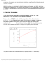
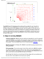
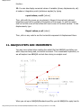
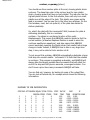
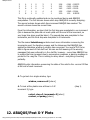
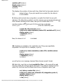
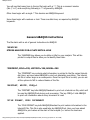
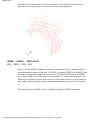
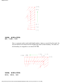
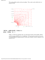
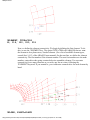
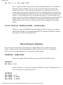
ABAQUS tutorial
EN175: Advanced Mechanics of
Solids
Division of Engineering
Brown University
ABAQUS tutorial
1. What is ABAQUS?
ABAQUS is a highly sophisticated, general purpose finite element program, designed primarily
to model the behavior of solids and structures under externally applied loading. ABAQUS
includes the following features:
Capabilities for both static and dynamic problems
The ability to model very large shape changes in solids, in both two and three
dimensions
A very extensive element library, including a full set of continuum elements,
beam elements, shell and plate elements, among others.
A sophisticated capability to model contact between solids
An advanced material library, including the usual elastic and elastic – plastic
solids; models for foams, concrete, soils, piezoelectric materials, and many others.
Capabilities to model a number of phenomena of interest, including vibrations,
coupled fluid/structure interactions, acoustics, buckling problems, and so on.
The main strength of ABAQUS, however, is that it is based on a very sound theoretical
framework As an practicing engineer, you may be called upon to make crucial decisions based
on the results of computer simulations. While no computer program can ever be guaranteed
free of bugs, ABAQUS is among the more trustworthy codes. Furthermore, as you will see if
you consult the ABAQUS theory manual, HKS developers really understand continuum
mechanics (since many of them are Brown Ph.Ds, this goes without saying). For this reason,
ABAQUS is used by a wide range of industries, including aircraft manufacturers, automobile
http://www.engin.brown.edu/courses/En175/Abaqustut/abaqustut.htm (1 of 37) [4/13/2007 11:12:12 AM]
ABAQUS tutorial
companies, oil companies and microelectronics industries, as well as national laboratories and
research universities.
ABAQUS is written and maintained by Hibbitt, Karlsson and Sorensen, Inc (HKS), which has
headquarers in Pawtucket, RI. The company was founded in 1978 (by graduates of Brown’s Ph.
D. program in solid mechanics), and today has several hundred employees with offices around
the world.
2. Tutorial Overview
In this tutorial, you will learn how to run ABAQUS/Standard, and also how to use
ABAQUS/Post to plot the results of a finite element computation.
First, you will use ABAQUS to solve the following problem. A thin plate, dimensions
, contains a hole of radius 1cm at its center. The plate is made from
steel, which is idealized as an elastic—strain hardening plastic solid, with Young’s
modulus E=210
GPa and Poisson’s ratio
. The uniaxial stress—strain
curve for steel is idealized as a series of straight line segments, as shown below.
The plate is loaded in the horizontal direction by applying tractions to its boundary.
http://www.engin.brown.edu/courses/En175/Abaqustut/abaqustut.htm (2 of 37) [4/13/2007 11:12:12 AM]
ABAQUS tutorial
The magnitude of the loading increases linearly with time, as shown.
You may recall that a circular hole in a plate has a stress concentration factor of about 3.
At time t=1
, therefore, the stress at point A should just reach yield (the initial
yield stress of the plate is 200MPa). At time t=3,
the load should be
enough to cause a significant portion of the plate to yield.
We will specifically request ABAQUS to print the state of the solid at time
t=1, t=2
and t=3
, to see the development of plasticity in
the plate.
Observe that the plate and the loading is symmetrical about horizontal and vertical axes
through the center of the plate. We only need to model ¼ of the plate, therefore, and
can apply symmetry boundary conditions on the the bottom and side boundaries. The
finite element mesh you will use for your computations is shown below. The elements
are plane stress, 4 noded quadrilaterials. Symmetry boundary conditions are applied as
shown, and distributed tractions are applied to the rightmost boundary.
http://www.engin.brown.edu/courses/En175/Abaqustut/abaqustut.htm (3 of 37) [4/13/2007 11:12:12 AM]
ABAQUS tutorial
The ABAQUS input file that sets up this problem will be provided for you. You will run
ABAQUS, and then use ABAQUS/Post to look at the results of your analysis. Next, you
will take a detailed look at the ABAQUS input file, and start setting up input files of your
own. After completing this tutorial, you should be in a position to do quite complex two
and three dimensional finite element computations with ABAQUS, and will know how to
view the results. We will continue using ABAQUS to solve various problems throughout
the rest of this course.
3. Steps in running ABAQUS
Create an input file. ABAQUS works by reading and responding to a set of commands
(called KEYWORDS) in an input file. The keywords contain the information to define the
mesh, the properties of the material, the boundary conditions and to control output from
the program. To see the ABAQUS input file for the plate problem, click here.
Run the program. On Windows NT, ABAQUS is controlled by typing commands into a
DOS type window.
Post processing. There are two ways to look at the results of an ABAQUS simulation.
You can ask the program to print results to a file, which you can look at with a text
editor. This is painful… Alternatively, you can use a program called ABAQUS/Post, which
can be used to plot various quantities that may be of interest.
We will begin this tutorial by running through all these stages with a pre-existing input
file, then look in more detail at how to set up an input file.
http://www.engin.brown.edu/courses/En175/Abaqustut/abaqustut.htm (4 of 37) [4/13/2007 11:12:12 AM]
ABAQUS tutorial
BEFORE RUNNING ABAQUS FOR THE FIRST TIME:
1. Open an MS/DOS window on your workstation (the command to open
the window is located in the Start menu on your toolbar).
2. Type mk_ABAQUS in the MS/DOS window. If the command executes
correctly, icons to start ABAQUS and to open the ABAQUS
documentation should appear on your desktop. In addition, a
directory called ABAQUS should be created in your home directory.
4. Downloading the sample ABAQUS input file.
1. If you completed the preceding step correctly , a directory called ABAQUS
should have been created in your home directory. Within your ABAQUS
directory, create a subdirectory called tutorial to store your input files and
results. ABAQUS will generate a vast number of output files, and to keep track of them,
it is convenient to keep all the files associated with a particular problem in one directory.
2. Download the example ABAQUS file. To do so, click here. You will see the input
file appear in the frame. Click anywhere on the frame, then select Save Frame As… from
the File menu on the top left hand corner of your browser. In the popup window, find
the directory called ABAQUS\tutorial , and save the file as tutorial.inp
3. Open tutorial.inp with a text editor. Take a quick look at the file and make sure
that it downloaded correctly.
4. Exit the text editor.
In future, you will create your own ABAQUS input file, by typing in appropriate keywords
with a text editor. The easiest thing to do will be to copy an existing file, and modify it
for other problems.
5. Running ABAQUS.
1. Double click the ABAQUS icon on your desktop. A window with a black
background should appear.
2. In the Abaqus Command window, change directories to ABAQUS\tutorial.
http://www.engin.brown.edu/courses/En175/Abaqustut/abaqustut.htm (5 of 37) [4/13/2007 11:12:12 AM]
ABAQUS tutorial
3. In the Abaqus Command window, type
Your Prompt > abaqus [return]
Identifier: tutorial [return]
User routine file: [return]
(The identifier should always be the name of the .inp file, without the .inp extension. The
user routine file will always be blank in anything we run in this course. It is needed only
when you start to write your own subroutines to run within ABAQUS). This starts the
ABAQUS program running. Note that the program runs in the background, so although
the prompt comes right back in the ABAQUS window, this does not mean the program
has finished. Note also that some special computations (e.g. using the *SYMMETRIC
MODEL GENERATION key) will cause ABAQUS to ask you some more questions during
execution.
4. Using explorer, or by opening a directory window, examine the files in the
directory tutorial. (Click here if you don’t know how to do this). You should see the
following files:
tutorial.inp
tutorial.dat
tutorial.log
tutorial.res
tutorial.bat
tutorial.sta
tutorial.msg
tutorial.fil
Fortunately, you can happily ignore most of these files. The only ones you need to look
at are tutorial.log, tutorial.sta, tutorial.msg and tutorial.dat. We will also use
tutorial.res and tutorial.fil later.
5. Open the file called tutorial.log with a text editor. You will see some information about
the time it took to for ABAQUS to complete execution. You should also see that the file
ends with
ABAQUS JOB tutorial COMPLETED
This means that ABAQUS is done and you can safely look at the results.
6. Open the file called tutorial.sta with a text editor. You will see columns of numbers,
headed by
http://www.engin.brown.edu/courses/En175/Abaqustut/abaqustut.htm (6 of 37) [4/13/2007 11:12:12 AM]
ABAQUS tutorial
SUMMARY OF JOB INFORMATION:
STEP INC ATT SEVERE EQUIL TOTAL TOTAL STEP INC OF DOF IF
DISCON ITERS ITERS TIME/ TIME/LPF TIME/LPF MONITOR RIKS
ITERS FREQ
This file is continuously updated by ABAQUS as it runs, and tells you how much of the
computation has been completed. You can monitor this file while ABAQUS is running. We
will discuss the meaning of data in this file in more detail later.
7. Open the file called tutorial.dat. This file contains all kinds of information about the
computations that ABAQUS has done. In particular, if ABAQUS encounters any problems
during the computation, error and warning messages will be written to this file. You
should first check the end of the file to see if the computation was successful. If the
program ran successfully, you should see a message saying
ANALYSIS COMPLETE
WITH 7 WARNING MESSAGES ON THE MSG FILE
JOB TIME SUMMARY
USER TIME (SEC) = 20.000
SYSTEM TIME (SEC) = 3.0000
TOTAL CPU TIME (SEC) = 23.000
WALLCLOCK TIME (SEC) = 36
The times listed above may differ on your computer, depending on the speed of the
processor and the memory available. The warning message is a bit scary, but is actually
nothing to worry about. We’ll see why it appears later.
You can explore the rest of this file to see what else is there. MAKE SURE YOU CLOSE
THE FILE BY EXITING THE TEXT EDITOR BEFORE PROCEEDING.
http://www.engin.brown.edu/courses/En175/Abaqustut/abaqustut.htm (7 of 37) [4/13/2007 11:12:12 AM]
ABAQUS tutorial
6. ABAQUS ERRORS
1. Next, we will deliberately introduce an error into the ABAQUS input file tutorial.inp, to
see what an unsuccessful run looks like. Open the file tutorial.inp with a text editor, and
change the line near the top that says
*RESTART, WRITE, FREQ=1
to
*RESTART, WONK, FREQ=1
Save the file in Text Only format. Now, repeat step 3 in Running ABAQUS to run ABAQUS
again. You will get an additional prompt as follows.
Old job files exist. Overwrite (y/n)? : y [return]
2. Check the files in the directory ABAQUS\tutorial again. This time, not all the files will
be there, because the run was unsuccessful.
3. Open the file called tutorial.log with a text editor. Note the error message there.
4. Open the file called tutorial.dat with a text editor. You will see that the end of the file
contains the following statements
THE PROGRAM HAS DISCOVERED 3 FATAL ERRORS
** EXECUTION IS TERMINATED **
END OF USER INPUT PROCESSING
JOB TIME SUMMARY
http://www.engin.brown.edu/courses/En175/Abaqustut/abaqustut.htm (8 of 37) [4/13/2007 11:12:12 AM]
ABAQUS tutorial
USER TIME (SEC) = 0.0000
SYSTEM TIME (SEC) = 0.0000
TOTAL CPU TIME (SEC) = 0.0000
WALLCLOCK TIME (SEC) = 2
This again shows that ABAQUS ran into trouble during execution. Search the file
backwards for the occurrence of ERROR to find the lines
***ERROR: UNKNOWN PARAMETER WONK
CARD IMAGE: *RESTART, WONK, FREQ=1
***NOTE: DUE TO AN INPUT ERROR THE ANALYSIS PRE-PROCESSOR HAS BEEN UNABLE TO
INTERPRET SOME DATA. SUBSEQUENT ERRORS MAY BE CAUSED BY THIS OMISSION
***ERROR: EITHER THE PARAMETER READ OR WRITE MUST BE SPECIFIED
CARD IMAGE: *RESTART, WONK, FREQ=1
***ERROR: PARAMETER FREQUENCY IS ONLY MEANINGFUL IF THE WRITE PARAMETER IS
ALSO SPECIFIED
CARD IMAGE: *RESTART, WONK, FREQ=1
This will tell you what part of the input file is causing problems, and if you are lucky, you
will understand the error message. Notice that ABAQUS programmers still seem to be
using punch cards. ABAQUS is coded in FORTRAN, too (for real).
5. Try another error. Change the line
*RESTART, WONK, FREQ=1
back to
*RESTART, WRITE, FREQ=1
This time, change the line
http://www.engin.brown.edu/courses/En175/Abaqustut/abaqustut.htm (9 of 37) [4/13/2007 11:12:12 AM]
ABAQUS tutorial
1031, 5.E-02, 5.E-02
to
1031, 5.E-02, -5.E-02
Re-run ABAQUS (don’t forget to save the .inp file first), then check the file tutorial.dat
again. ABAQUS really freaks out with this problem. You should see 96 fatal errors. If you
have no life, you might like to try and see if you can produce more errors than this by
inserting a single character in the input file.
6. Before proceeding, correct the input file, and re-run ABAQUS. Check the .dat file and .
log file to make sure that the job ran properly.
7. Running ABAQUS/Post.
1. If you have not already done so, run ABAQUS with a correct input file tutorial.
inp. You can download an error free copy of the tutorial file by clicking here if you
need to.
2. To run ABAQUS/Post, you will need to start a program called Exceed first. Find
Exceed on the Start menu of your desktop, and select it to start it running. A
window will be displayed briefly and an icon should appear on your toolbar if the
program started properly.
3. Make sure you have an ABAQUS command window open, set to the appropriate
directory. In the ABAQUS command window, type
abaqus post
4. A window should appear, which will be used to display results of the ABAQUS
run. To do so, you type commands in the bottom left hand corner of the window.
We will try a few useful commands in the next section
8. Online help with ABAQUS/Post
In the ABAQUS/Post window, type
help [return]
http://www.engin.brown.edu/courses/En175/Abaqustut/abaqustut.htm (10 of 37) [4/13/2007 11:12:12 AM]
ABAQUS tutorial
A black window will open, with a list of ABAQUS/Post commands. To get help with
any command, just type the command name.
9. ABAQUS/Post Mesh and Boundary Condition Display
1. The first step is to read the results of an analysis into ABAQUS/Post. Our
example simulation created two files that can be read into ABAQUS/Post:
tutorial.res
tutorial.fil
The file named tutorial.res is called a `restart file’ (the file always has .res
extension). This file contains full information about the analysis. The restart file is
most useful if you want to plot the finite element mesh, or contours of stress,
displacement, etc. The file named tutorial.fil is called a `results file’ (the file
always has a .fil extension). This file contains data that were specifically requested
in the ABAQUS input file. The results file is most useful when you want to create xy plots of stress-v-time, stress-v-strain, or similar.
To read the restart file, type
restart, file=tutorial [return]
A black window will pop up, with lots of interesting information in it. Ignore the
useful information and type [return] anywhere in the window. When you read
the restart file with this syntax, all quantities displayed will represent
the state of the solid at the very end of the analysis. We will see how to
display data at other times lower down.
2. Now, we can start plotting things. Type
draw [return]
in the ABAQUS/Post window. This will plot the undeformed finite element mesh.
3. To display node numbers with the mesh, type
set, n numbers=on [return]
http://www.engin.brown.edu/courses/En175/Abaqustut/abaqustut.htm (11 of 37) [4/13/2007 11:12:12 AM]
ABAQUS tutorial
draw [return]
4. To display element numbers with the mesh, type
set, el numbers=on [return]
draw [return]
5. To zoom in and out of the mesh, right click on the mesh and drag the mouse
left or right, while continuing to hold the mouse button down.
6. To move the mesh around on the window, center click on the mesh and drag
the mouse.
7. To rotate the FEM mesh, left click and drag the mouse, and/or left click with the
shift key held down while dragging the mouse. (This is not too helpful with a 2D
mesh, but is very useful in 3D).
8. Another useful way to zoom in on a small region is
zoom, cursor [return]
Now, click on the mesh at two points. The two points define opposite corners of a
box. When you type
draw [return]
the region within the box will be scaled to fit the full window.
9. To turn off element numbers and node numbers again, type
set, el numbers=off, n numbers=off [return]
draw [return]
10. To get back to the original view of the mesh, type
reset, all [return]
draw [return]
11. Another useful option for checking a mesh is
set, fill=on [return]
draw [return]
http://www.engin.brown.edu/courses/En175/Abaqustut/abaqustut.htm (12 of 37) [4/13/2007 11:12:12 AM]
ABAQUS tutorial
report elements [return]
Now, click on any element in the mesh, and information concerning the element
will be displayed at the bottom of the window. To exit this option, click on the little
X at the bottom left hand corner of the black window. The key
report nodes [return]
tells you about nodes.
12. You can also display the boundary conditions applied to the mesh, by typing
set, bc display=on
draw
If you have superb eyesight, you will see some little dots on the left and bottom
edges of the mesh. Zoom in, and you will see arrows representing the constraints
applied to the bottom of the mesh.
13. Before proceeding to the next section, type
reset, all [return]
10. ABAQUS/Post Field Plots
If you have not already done so, start up ABAQUS/Post and read in tutorial.res
1. To view the deformed shape of the solid after loading, type
draw, displaced [return]
You can use the mouse to drag the mesh away from the text message that
appears on the window. Note that the deformation is grossly exaggerated to show
it clearly: the scale factor is displayed on the text message.
2. Recall that, by default, ABAQUS/Post will display the state of the solid at the
very end of whatever load history was specified in the input file. To see the results
at other times, you can type
restart, step=1 [return]
draw, displaced [return]
http://www.engin.brown.edu/courses/En175/Abaqustut/abaqustut.htm (13 of 37) [4/13/2007 11:12:12 AM]
ABAQUS tutorial
This will display the deformed mesh at the end of the first load step. In this case,
the deformed mesh doesn’t look very different at the end of the first step, but you
should see a message in the bottom left hand corner of the screen telling you that
the current step is 1.
3. To remove the undeformed mesh, type
set, undeformed=off [return]
draw, displaced [return]
4. To see the actual displacements (without magnification), type
set, d magnification=1.0 [return]
draw, displaced [return]
5. To plot a contour of the horizontal component of stress
, type
contour, v=s11 [return]
6. To show the contours as solid colors instead of lines, type
set, fill=on [return]
contour, v=s11 [return]
7. To remove the mesh to see the contours more clearly, type
set, outline=perimeter[return] or set, outline=off [return]
contour, v=s11 [return]
8. To turn the mesh back on again, type
set, outline=element [return]
9. You can plot all field quantities the same way. Examples include
v=s22; v=s12, v=s33, etc plot various stress components
v=mises plots von Mises stress.
10. You can do vector plots too. For example
vector plot, v=u [return]
shows arrows whose length and orientation correspond to the vector displacement
at each node. Obviously, you can only do a vector plot of a vector valued
http://www.engin.brown.edu/courses/En175/Abaqustut/abaqustut.htm (14 of 37) [4/13/2007 11:12:12 AM]
ABAQUS tutorial
function…
11. You can also display numerical values of variables (stress, displacements, etc)
at nodes or integration points (whichever applies) by typing
report values, v=s11 [return]
Then, click with the mouse on any element. Values of stress at each element
integration point will be printed at the bottom of the screen. To exit this option,
click on the little cross at the bottom left hand corner of the black window. To see
displacements, type
Report values, v=u1 [return]
Then, click on any node to see the horizontal component of displacement there.
11. ABAQUS STEPS AND INCREMENTS
You may have noticed when reading the restart file that ABAQUS was telling you
which step was being read, and which increment. This is somewhat mysterious, so
we will explore how ABAQUS controls time during an analysis next.
When you set up an ABAQUS/Standard input file, you tell ABAQUS to apply load to
http://www.engin.brown.edu/courses/En175/Abaqustut/abaqustut.htm (15 of 37) [4/13/2007 11:12:12 AM]
ABAQUS tutorial
a solid in a series of steps. For the hole in a plate problem, we applied load to the
to t=1
(step 1); from t=1
to
solid in three steps, from t=0
t=2
(step 2) and finally from t=2
to t=3
. ABAQUS will
always print out the state of the solid at the end of each step. When you type
restart, step=2
in ABAQUS/Post and then plot something, you will see the
state of the solid at the end of step 2 – in this case, at time t=2
.
Let’s check this out. We will compare the plastic zone size in the solid
at times t=1
, t=2
and t=3
.
1. If you have not already done so, start up ABAQUS/Post, and read
in tutorial.res.
2. Now, we will open up three windows to display all three times on
the same picture. Type
window, name=first, maximum=(0.4,1.0),
minimum=(0.0,0.6) [return]
window, name=second, maximum=(0.7,0.7),
minimum=(0.3,0.3) [return]
window, name=third, maximum=(1.0,1.0),
minimum=(0.6,0.6) [return]
Here, the maximum=… specifies the coordinates of the upper right
hand corner of the window, while the minimum specifies the lower
left hand corner. You can also use window, name=..., cursor and
then click on the screen with the mouse to define the corners of the
window, but don’t try that now or else you will have an extra window
open that you don’t want.
3. Now, we will plot contours of plastic strain at
t=1¸t=2
and t=3
in the three
windows. Type
window, name=first [return]
set, fill=on [return]
restart, step=1 [return]
contour, v=pemag [return]
window, name=second [return]
restart, step=2 [return]
contour, v=pemag [return]
window, name=third [return]
restart, step=3 [return]
http://www.engin.brown.edu/courses/En175/Abaqustut/abaqustut.htm (16 of 37) [4/13/2007 11:12:12 AM]
ABAQUS tutorial
contour, v=pemag [return]
You should see three contour plots at the end, showing plastic strain
contours. The deep blue color is the contour level for zero plastic
strain, showing areas that have not yet yielded. The red color has the
highest plastic strains. In the first window, there will only be a small
plastic zone at the edge of the hole. This plastic zone grows as the
load is increased. You can see this in the other two windows. On the
third window, most, but not quite all, of the plate has started to
deform plastically.
So, what’s the deal with the increments? Well, because the plate is
deforming plastically, this is a nonlinear
problem – the stress is a nonlinear function of the nodal
displacements. This means that ABAQUS needs to iterate to find the
correct solution (a Newton-Raphson iteration is used to solve the
nonlinear equilibrium equations), and also means that ABAQUS
cannot accurately compute the plastic strain that results from a large
change in loads. Indeed, if ABAQUS tries to take a very large time
step, it may not be able to find a solution at all.
To get around this problem, ABAQUS automatically subdivides a large
time step into several smaller `increments’ if it finds that the solution
is nonlinear. This process is completely automatic, and ABAQUS will
always take the largest possible time increments that will reach the
end of the step and still give an accurate, convergent solution. You
don’t know a priori how many increments ABAQUS will take.
You can find out, however, by looking at some of the output files.
You can look at tutorial.sta, for example which shows the following
information:
SUMMARY OF JOB INFORMATION:
STEP INC ATT SEVERE EQUIL TOTAL TOTAL STEP INC OF
DOF
IF
DISCON ITERS ITERS TIME TIME TIME
MONITOR RIKS
1
1
1
0
4
4
1.00
1.00
1.000
2
1
2
0
4
4
1.25
0.250 0.2500
2
2
1
0
3
3
1.50
0.500 0.2500
2
3
1
0
4
4
1.88
0.875 0.3750
2
4
1
0
4
4
2.00
1.00
0.1250
3
1
3
0
5
5
2.06
0.0625 0.06250
3
2
1
0
3
3
2.13
0.125 0.06250
3
3
1
0
3
3
2.19
0.188 0.06250
http://www.engin.brown.edu/courses/En175/Abaqustut/abaqustut.htm (17 of 37) [4/13/2007 11:12:12 AM]
ABAQUS tutorial
3
3
3
3
3
4
5
6
7
8
1
1
1
1
1
0
0
0
0
0
3
3
4
4
1
3
3
4
4
1
2.28
2.42
2.63
2.95
3.00
0.281
0.422
0.633
0.949
1.00
0.09375
0.1406
0.2109
0.3164
0.05078
This file is continually updated and can be monitored during and ABAQUS
computation. The first column shows which step ABAQUS is currently analyzing.
The second column shows which time increment ABAQUS has reached. The
seventh column shows the current time.
From this information, we learn that the first step was completed in one increment
(this is because the plate did not reach yield until the end of the increment, so
very large time steps could be taken). The second step was completed in four
increments, and the third step was completed in 8 increments.
The file named tutorial.msg contains much more information concerning the
increments used, the iterative process, and the tolerances that ABAQUS has
applied to determine whether a solution has converged. You need a Ph.D to be
able to figure most of that stuff out. We can see the meaning of the warning
messages that were referred to in the .dat file, however – every time ABAQUS has
to reduce the time increment due to convergence problems, a warning message is
printed to the .msg file. This is nothing to worry about – everything is working
perfectly.
ABAQUS prints information concerning the state of the solid to the .res and .fil files
at the end of each increment.
4. To go back to a single window, type
window, remove=all [return]
4. To look at the plastic zone at time t=2.42
increment 5), type
restart, step=3, increment=5 [return]
contour, v=pemag [return]
12. ABAQUS/Post X-Y Plots
http://www.engin.brown.edu/courses/En175/Abaqustut/abaqustut.htm (18 of 37) [4/13/2007 11:12:12 AM]
(step 3,
ABAQUS tutorial
ABAQUS/Post can also be persuaded to plot variations of stress, displacement, etc
with position within the solid, or can display stresses, strains, etc as a function of
time at a point in the solid, or can even plot stress as a function of strain (or
anything else, for that matter). The procedure to do this is rather weird.
We will begin by plotting x-y graphs of field quantities with position in the solid.
If you have not already done so, start up ABAQUS/Post and read in tutorial.res.
1. First, we will plot the variation of
with distance along the base.
First, we define a set of data known as a `curve,’ by using the path keyword
path, node list, variable=s22, name=syy, distance, absolute
[return]
>119 [return]
>120 [return]
>121 [return]
… Continue typing in numbers in increasing order until you get to
>131 [return]
>[return]
This procedure defines a set of (x,y) data pairs at each node entered in the list.
The x coordinate is zero at the first node, and is incremented by the distance
between nodes for each subsequent node in the list. The y coordinate is s22.
The group of all the data pairs generated by this command has been given the
name `syy’. To find the list of nodes you need for the path of interest, it is
simplest to plot the mesh with node numbers.
2. Now, we can plot these (x,y) data points
display curve [return]
> syy [return]
> [return]
3. We can define and plot other data on the same graph. Instead of typing in a list
of nodes this time, we will use the `generate’ key to generate the list
automatically
http://www.engin.brown.edu/courses/En175/Abaqustut/abaqustut.htm (19 of 37) [4/13/2007 11:12:12 AM]
ABAQUS tutorial
path, node list, generate, variable=s11, name=sxx, distance, absolute
[return]
>119,131,1 [return]
>[return]
display curve [return]
> syy [return]
> sxx [return]
> [return]
Do you see anything wrong with the value of sxx at x=0? Why? What could cause
this error?
4. For a 3D analysis, you can ask for curves to be generated along a straight line,
instead of entering a list of node numbers. To produce the results we want here,
we would enter
path, start=(0.01,0.0), end=(0.05,0.0), variable=s22,
name=syy, distance, absolute [return]
Unfortunately, this does not work in 2D, so you are stuck entering node lists.
5. There are various commands you can use to change the appearance of the x-y
plot. For example
graph axes, x title=x, y title=normal stress, x grid=solid, y grid=solid
[return]
display curve [return]
>syy [return]
> [return]
Unfortunately, no matter how hard you try, x-y plots output from ABAQUS/Post
look pretty shitty. If you want publication quality output, your best bet is to print
the data and plot it with something else, or print out a postscript file and then edit
it with another graphics package.
6. The path defined by the node list need not be a straight line. For example, to
plot the variation of Mises stress around the perimeter of the hole, use
path, node list, generate, variable=mises, name=sm, distance, absolute
[return]
>119,1919,100 [return]
> [return]
http://www.engin.brown.edu/courses/En175/Abaqustut/abaqustut.htm (20 of 37) [4/13/2007 11:12:12 AM]
ABAQUS tutorial
graph axes, x title=s, y title=mises stress [return]
display curve [return]
>sm [return]
> [return]
7. You can also manipulate the data in an X-Y curve. For example, we could
compute the resultant vertical force acting on a section of the bottom boundary by
integrating the normal stress distribution
To do this with ABAQUS/Post, use
define curve, name=result, operation=integrate [return]
>syy [return]
This generates a new curve, named result, which is the integral of syy. To plot it,
type
display curve [return]
> result [return]
> [return]
The curve should theoretically cross zero at x=0.04
,
but
as you see, there is a slight error in the finite element computation. This error
could be reduced by using a finer finite element mesh. It is always worth doing
checks like this to test the accuracy of your numerical solutions.
8. ABAQUS/Post will also do another kind of x-y
plot. Instead of plotting
variables as a function of position, you can plot variables as a function of time, as
the load is applied to the solid. For example, we will plot the time variation of
at the point near (0.01,0.0) (this is on the edge of the hole). We are plotting
results from a restart file (remember that we read in the restart file right at the
beginning of this section), so the stresses are defined only at the integration
points within each element, and are not available at the nodes. By drawing the
mesh with element numbers, we see that the element closest to our point of
interest has number 19. This is a 4 noded element, and so has 4 integration
points. We will plot the stress at integration point number 1, which is closest to
the point of interest.
read curve, name=stress, element=19, integration point=1,
http://www.engin.brown.edu/courses/En175/Abaqustut/abaqustut.htm (21 of 37) [4/13/2007 11:12:12 AM]
ABAQUS tutorial
variable=s22 [return]
display curve [return]
>stress [return]
>[return]
This displays the variation of stress with time. Note that the time scale starts at
t=1
instead of zero. If you plot results from a restart file, the state at
t=0
is not available.
9. History plots are best done using data in a results file (that’s the one with
extension .fil) rather than a restart (.res) file, because you can access stresses and
other element variables at the nodes, and you can include data at t=0
. To
read the variation of
x=0.01, y=0
at node 119 (this node has coordinates
) from the results file, type
results file, file=tutorial [return]
read curve, name=newstres, node=119, variable=s22 [return]
display curve [return]
>newstres [return]
>[return]
Now, the stress at t=0
is included.
10. Variables are available in the results file only if they were specifically
requested in the input file. For example, if you try
read curve, name=newmises, node=119, variable=mises
[return]
display curve [return]
> newmises [return]
> [return]
you will get an error message, because Mises stresses weren’t stored.
11. Note that, now that you typed results file, file=… all curves will be read
from the results file until you specify otherwise. To go back to reading from the
restart file, and then read the Mises stress from an integration point, type
set, history=restart file [return]
read curve, name=nm, element=19, integration point=1,
variable=mises [return]
display curve [return]
> nm [return]
http://www.engin.brown.edu/courses/En175/Abaqustut/abaqustut.htm (22 of 37) [4/13/2007 11:12:12 AM]
ABAQUS tutorial
> [return]
12. Let’s go back to reading curves from the results file. Type
set, history=results file [return]
13. We can also plot the variation of stress with strain at a node (we’ll try 1919
this time, since there is a nice big plastic strain there), instead of plotting stress as
a function of time. To do this, we first read stress-v-time and strain-v-time as two
separate curves, and then combine them to create stress-v-strain. First, read the
stress-v-time curve at node 1919 (we’ll replace the old curve named newstres)
read curve, name=newstres, node=1919, variable=s11
[return]
> Overwrite [return]
Now, read the strain –v- time curve
read curve, name=strain, variable=e11, node=1919 [return]
Now, we will create a stress-v-strain graph
Define curve, name=strsstrn, operation=combine [return]
> strain [return]
> stress [return]
> [return]
display curve [return]
> strsstrn [return]
> [return]
The y axis of the first curve (strain) becomes the x
axis of the new curve
(strsstrn), while the y axis of the second curve (stress) becomes the y axis of
the new curve.
Check the initial the stress—strain curve to make sure that it is correct. The
material point at node 1919 is subjected to uniaxial stress, so the stress—strain
curve should (if the numerical analysis is accurate) match the uniaxial stress—
strain curve for the material.
13. Printing output from ABAQUS/Post
It takes three steps to print out results from ABAQUS/Post.
http://www.engin.brown.edu/courses/En175/Abaqustut/abaqustut.htm (23 of 37) [4/13/2007 11:12:12 AM]
ABAQUS tutorial
If you have not already done so, start ABAQUS/Post and read in tutorial.res
1. First, type
set, hard copy=on
in the ABAQUS/Post window. With this option set, every time you enter a
command such as draw, contour, display curve… that changes the ABAQUS/
Post display, the new display is also output to a device neutral file called tutorial.
mpl. This file will later be converted to a form that can be printed.
2. As an example, we will draw the mesh, the displaced mesh, and an x-y plot of
stress.
draw [return]
draw, displaced [return]
path, node list, generate, variable=s22, name=splot,
distance, absolute [return]
> 119,131,1 [return]
>[return]
display curve [return]
> splot [return]
> [return]
3. Once you are done plotting all the graphs you want, type
set, hard copy=off [return]
Any further plots you make will not be output to the .mpl file. For example, if you
now type
contour, v=mises [return]
the contour plot will not be printed.
4. Now, we will exit ABAQUS/Post
end [return]
5. To print our graphs, we now need to turn the tutorial.mpl file into a postscript
file that can be sent to the printer. To do this, go the the ABAQUS command
window, and type
abaqus plot device=cps job=tutorial
http://www.engin.brown.edu/courses/En175/Abaqustut/abaqustut.htm (24 of 37) [4/13/2007 11:12:12 AM]
ABAQUS tutorial
If this doesn't work you should try
p:\abaqus\abaqus plot device=cps job=tutorial
The program will ask you a number of questions concerning the format you wish
to adopt for the printed file. The appropriate responses should be obvious – in
most cases, you should accept the default. Finally, when you have answered all
the questions, ABAQUS/Plot will produce a postscript file, named tutorial.ps.
(If you asked ABAQUS/Plot to print each page to a separate file, it will produce
three files, named tutorial_page_1.ps, tutorial_page_2.ps and tutorial_page_3.ps).
You can view the file using Ghostview, or convert it into a pdf file using Adobe
Distiller, and then view the file with Adobe Acrobat Reader or Adobe Acrobat
Exchange. There is also some software that will read in postscript files and allow
you to edit them and print them out in another format. The ABAQUS plots on this
web site were read into Micrografx Designer, edited, and then printed out as .gif
files. Finally, you can print the postscript file on any postscript printer. On the NT
workstations in Prince Lab, you can print a ps file by dragging it onto the icon
labelled PSPrint on your desktop.
14. A detailed look at an ABAQUS input file
We are ready to start learning how to use ABAQUS itself. First, we will look at the input
file for the hole-in-a-plate problem, and then start doing some simple exercises to learn
how to set up new problems.
Before looking at the input file, you may find it helpful to review the problem being
solved.
You can either click here to see the full input file, with detailed comments, or read below
to see an explanation of each command in the file. You can find detailed documentation
about each keyword in volume III of the ABAQUS/Standard user manual, or in the online
documentation.
The input file is divided into the following general sections
1.
2.
3.
4.
5.
General ABAQUS commands, controlling printing, and naming the analysis
Mesh generation commands
Material property definition
Time independent Boundary condition specifications
Commands specifying time varying loads, and controlling ABAQUS time steps and
increments.
http://www.engin.brown.edu/courses/En175/Abaqustut/abaqustut.htm (25 of 37) [4/13/2007 11:12:12 AM]
ABAQUS tutorial
You will see that many lines in the.inp file begin with a **. This is a comment marker
(like /* in C) and everything following a ** is ignored by ABAQUS.
Other lines begin with a single * This denotes an ABAQUS keyword.
Some lines begin with numbers or text. These are data lines, as required by ABAQUS
keywords.
General ABAQUS instructions
The file starts with a set of general instructions to ABAQUS
*HEADING
STRESS ANALYSIS FOR A PLATE WITH A HOLE
The *HEADING key allows you to define a title for your analysis. This will be
printed in output files to allow you to identify them later.
*PREPRINT, ECHO=YES, HISTORY=YES, MODEL=YES
The *PREPRINT key controls what information is printed to the file named tutorial.
dat. Here, we have asked ABAQUS to print out absolutely everything. The tutorial.
dat file is rather large as a consequence. Once the input file is correct, you can set
all the options to NO to reduce thesize of the file.
*RESTART, WRITE, FREQ=1
The *RESTART key tells ABAQUS/Standard to print out a tutorial.res file, which will
be used by ABAQUS/Post during post processing. The key FREQ=1 tells ABAQUS
to print out information about every increment in Load
*FILE FORMAT, ZERO INCREMENT
The *FILE FORMAT key tells ABAQUS/Standard to print certain information to the
tutorial.fil file. This file is also used later by ABAQUS/Post. Here, we have asked
ABAQUS to print values at the start of the analysis (i.e. before the loads are
applied.
http://www.engin.brown.edu/courses/En175/Abaqustut/abaqustut.htm (26 of 37) [4/13/2007 11:12:12 AM]
ABAQUS tutorial
Mesh Generation
Next, there follow a set of lines defining the mesh. Nodes are generated first, then the
element type and element connectivity are specified.
*NODE
101, 0.0, 0.0
119, 1.0E-02, 0.0
1919, 0.0, 1.E-02
131, 5.E-02, 0.0
1031, 5.E-02, 5.E-02
1931, 0.0, 5.E-02
First, we define five key nodes, which will be used to generate further nodes later. The
positions of these nodes are shown in the picture above. The *NODE keyword starts node
definition. On the lines below, enter the node number, and x,y (and z for 3D) coordinates.
http://www.engin.brown.edu/courses/En175/Abaqustut/abaqustut.htm (27 of 37) [4/13/2007 11:12:12 AM]
ABAQUS tutorial
Note that the first node (number 101) is not actually in the solid at all. It is used when
generating the mesh, but is not used in the finite element computation.
*NGEN, LINE=C, NSET=HOLE
119, 1919, 100, 101
Now, we use the NGEN command to generate further nodes. First, we generate a line of
nodes around the perimeter of the hole. The LINE=C option of NGEN tells ABAQUS that
the nodes you generate should be on a circular arc. The NSET=HOLE option of NGEN
gives a name (HOLE) to all the nodes on this boundary. We will use this name later. The
following line specifies the first node on the arc, the last node on the arc, the increment in
node numbers between adjacent nodes, and the node number at the center of the circular
arc.
(this must already be defined -- here, we defined it using the *NODE command)
http://www.engin.brown.edu/courses/En175/Abaqustut/abaqustut.htm (28 of 37) [4/13/2007 11:12:12 AM]
ABAQUS tutorial
*NGEN, NSET=OUTER
131, 1031, 100
Now, we generate nodes on the right hand boundary. Again, we specify the first node, the
last node and the increment between neighboring nodes on this boundary. The nodes on
this boundary are assigned to a set named OUTER.
*NGEN, NSET=OUTER
1031, 1931, 100
http://www.engin.brown.edu/courses/En175/Abaqustut/abaqustut.htm (29 of 37) [4/13/2007 11:12:12 AM]
ABAQUS tutorial
The next key defines nodes on the top boundary. These nodes are also added to the set
named OUTER
*NFILL, NSET=PLATE, BIAS=0.8
HOLE, OUTER, 12, 1
Finally, we fill in the remaining nodes, by connecting the nodes on the boundary HOLE
and the boundary OUTER in a set of radial lines. To learn about how this keyword works,
consult the ABAQUS/Standard manual. All the nodes within the solid are assigned to a set
named PLATE.
http://www.engin.brown.edu/courses/En175/Abaqustut/abaqustut.htm (30 of 37) [4/13/2007 11:12:12 AM]
ABAQUS tutorial
*ELEMENT, TYPE=CPS4
19, 119, 120, 220, 219
Next, we define the element connectivity. We begin by defining the first element. To do
this, we use the *ELEMENT key. The option TYPE=CPS4 tells ABAQUS that we want
the element to be a plane stress, 4 noded element. (For a list of available element types,
consult Sect 14.1.3 of the ABAQUS user manual). On the next line, we define the element
connectivity. The first number is the element number. The next four numbers are the node
numbers, entered in order going counterclockwise around the element. You can enter
connectivity for as many elements as you wish, one line at a time, following the
*ELEMENT keyword. If you wanted to, you could enter connectivities for each element by
hand.
*ELGEN, ELSET=PLATE
http://www.engin.brown.edu/courses/En175/Abaqustut/abaqustut.htm (31 of 37) [4/13/2007 11:12:12 AM]
ABAQUS tutorial
19, 12, 1, 1, 18, 100, 100
Now, we generate element connectivity for all the remaining elements. The *ELGEN key
generates a block of elements, one row at a time. The first number specifies the first
element in the first row. This element must already have its connectivity defined. The
second number is the number of elements in each row. The third number is the increment
between neighboring element numbers in the row. The fourth number is the change in node
numbers of corresponding nodes between neighboring elements. The fifth number is the
number of rows to be defined (including the first one). The third number is the increment in
element numbers from one row to the next. The final number is the increment in node
numbers from one row to the next. All the elements have been assigned to a set named
PLATE
*SOLID SECTION, MATERIAL=STEEL, ELSET=PLATE
Finally, we need to tell ABAQUS what each element is made of. To do this, we assign a
material named STEEL to the elements named PLATE, using the *SOLID SECTION key.
The properties of STEEL are defined below.
Material Property Definition
We need to specify the behavior of the material we called STEEL. Here, we define an isotropic
elastic -- plastic material, with Young's modulus 210 GPA and Poisson's ratio 0.31, and a plastic
strain -v- stress curve approximated by a set of piecewise linear segments
*MATERIAL, NAME=STEEL
Specify the Young's modulus and Poisson's ratio with the *ELASTIC keyword
*ELASTIC
210.E09, 0.31
Specify yield stress -v- plastic strain with the *PLASTIC keyword. The data pairs are (true
stress, true strain) for a uniaxial tension test
*PLASTIC
200.2E06, 0.0
246.0E06, 0.0235
294.0E06, 0.0474
http://www.engin.brown.edu/courses/En175/Abaqustut/abaqustut.htm (32 of 37) [4/13/2007 11:12:12 AM]
ABAQUS tutorial
374.0E06, 0.0935
437.0E06, 0.1377
480.0E06, 0.18
Time independent boundary conditions
Next, we need to specify how the plate is loaded. This is done in two stages. Any boundary
conditions which do not vary with time are defined before we start the analysis. In this case, the
left hand boundary and the bottom boundary are symmetry boundaries.
*NSET, NSET=BOTTOM, GENERATE
119, 131, 1
*NSET, NSET=LEFT, GENERATE
1919, 1931, 1
First, we define a node set which contains all the nodes on the top and bottom boundary,
using the *NSET, GENERATE key. The syntax for the line following is first node number
in the set, last node number in the set increment between node numbers in the set
*BOUNDARY
BOTTOM, YSYMM
LEFT, XSYMM
Now, we define the boundary conditions. The node set BOTTOM is has symmetry about
the Y=0 axis imposed, and the node set LEFT has symmetry about the X=0 plane imposed.
Information defining time varying loads
Next, we define some information about the loading. To load the plate, we will apply a distributed
load right hand boundary. We need to define the elements on this boundary. We generate and
element set named EDGE using the *ELSET, GENERATE key. This works just like the *NSET,
GENERATE key.
*ELSET, ELSET=EDGE, GENERATE
http://www.engin.brown.edu/courses/En175/Abaqustut/abaqustut.htm (33 of 37) [4/13/2007 11:12:12 AM]
ABAQUS tutorial
30, 830, 100
We proceed to define some information about the time variation of the loads. Here, we will
ramp the loads steadily from zero at time t=0 to a maximum at time t=3.0 We define this
time variation in an object known as an AMPLITUDE. Here, we have named the
AMPLITUDE HIST, and have told ABAQUS that the x coordinates of the data pairs
following represent total time. Then, we enter pairs of numbers (time, load magnitude) with
four pairs to each line (you can have fewer than four pairs on the last line).
*AMPLITUDE, NAME=HIST, TIME=TOTAL TIME
0.0,0.0, 1.0,1.0, 2.0,2.0, 3.0,3.0
Load Step Definition
In doing the analysis, we will apply the load in a series of STEPS. The first load step lasts from
time t=0 to time t=1. ABAQUS will always print out the state of the plate at the end of a load
step, so we will have some results that show the plate just starting to yield at the edge of the hole
at time t=1. The second load step lasts from time t=1 to t=2. The plastic zone should grow
significantly during this step. The last load step lasts from time t=2 to t=3. The whole plate should
begin to yield towards the end of this load step.
First Load Step
*STEP,AMPLITUDE=RAMP
To start the analysis, we use the *STEP key.The AMPLITUDE=RAMP key is rather
confusing here -- in the STEP key, the AMPLITUDE does not refer to a predefined history
of load as described above, but tells ABAQUS how to apply the load during this time step.
If you specify AMPLITUDE=RAMP, the load is applied smoothly, while if you say
AMPLITUDE=STEP, the load is applied at once.
*STATIC
1.0,1.0
We tell ABAQUS that this is a quasi--static analysis. The stress fields are in static
http://www.engin.brown.edu/courses/En175/Abaqustut/abaqustut.htm (34 of 37) [4/13/2007 11:12:12 AM]
ABAQUS tutorial
equilibrium throughout the history of load. To choose a static analysis, use the *STATIC
key word. The first number on the following line suggests an initial value for the time
increment that ABAQUS should take while calculating the deformation in this step. Since
we expect the plate to deform elastically in this step, it makes sense to take a time
increment equal to the step size -- ABAQUS should be able to go straight to the solution at
the end of the step, without taking little steps to get there. The second number specifies the
time interval for this load step. The step starts at time t=0 and ends at time t=1, so the time
interval is 1.
Two additional optional parameters are also available - the third number specifies a
minimum value for the time increment, and the last number specifies a maximum value.
We have not used these parameters here.
*DLOAD, AMPLITUDE=HIST
EDGE, P2, -82.E06
Now we specify the loading applied to the plate. We select distributed loads(pressure)
acting on face 2 (P2) of all the elements in set EDGE. We take the load magnitude to be 82
MPA, so that when it is scaled by HIST, the stress reaches 82MPA at time t=1. Note that,
by definition, *DLOAD defines pressure (i.e. compressive normal stress) to be positive, so
we apply tensile loading by making the pressure negative.
*EL FILE, POSITION=AVERAGED AT NODES
S,E
Next, we specify what variables we'd like printed to the history file for post processing. We
are going to print all stress components (S) and strain components (E). These variables are
normally only computed at element integration points, so we use the *EL FILE keyword to
ask ABAQUS to print them to a file. However, we are really interested in values of stress
and strain at the nodes in this case, so we set the POSITION=AVERAGED AT NODES
flag to have ABAQUS calculate the varibles at nodes.
*END STEP
This keyword ends the step definition.
http://www.engin.brown.edu/courses/En175/Abaqustut/abaqustut.htm (35 of 37) [4/13/2007 11:12:12 AM]
ABAQUS tutorial
Second Load Step
*STEP,AMPLITUDE=RAMP
*STATIC
1.0,1.0
The second step lasts from time t=1 to t=2, so the step time is 1 sec again. We ask
ABAQUS to try to get to the end of the step in 1 increment, using an increment time of 1
sec. This is a bit optimistic. There is a lot of plasticity in this step, so ABAQUS will
actually end up taking several load increments.
*DLOAD, AMPLITUDE=HIST
EDGE, P2, -82.E06
The distributed load magnitude is 82MPa again, since it gets scaled by the load factor in
HIST to bring it to the correct magnitude. (HIST=2 at time 2 sec, so HIST*82=166MPa).
*EL FILE, POSITION=AVERAGED AT NODES
S,E
*END STEP
Third load step
You should get the idea by now!
*STEP,AMPLITUDE=RAMP
*STATIC
1.0,1.0
*DLOAD, AMPLITUDE=HIST
EDGE, P2, -82.E06
*EL FILE, POSITION=AVERAGED AT NODES
S,E
*END STEP
http://www.engin.brown.edu/courses/En175/Abaqustut/abaqustut.htm (36 of 37) [4/13/2007 11:12:12 AM]
ABAQUS tutorial
15. Setting up your own ABAQUS input file
To help you set up your own input files, a template file has been provided for you. Click here to
see it, and use your browser download it, following the same procedure that you used to download
tutorial.inp. The template file reminds you of the general layout for the input file, and contains a
list of useful keywords in each section. You can type ABAQUS commands directly into the
template file if you wish, or use it as a quick reference list of keywords.
To learn how to use each keyword, you will need to refer to the ABAQUS documentation. The
following sources of information are available:
1. Online documentation: select Start on the toolbar, select Programs on the popup menu,
select ABAQUS and then ABAQUS documentation. The documentation includes
instructions for using the documentation… One word of warning – make sure you only
refer to the ABAQUS/Standard manual. We will not be using ABAQUS/Expicit.
2. There are several hard copies of the ABAQUS manuals in the Prince Lab Computer
Balcony. Do not remove the manuals from the balcony.
3. ABAQUS comes with an extensive set of example problems. The examples are described
in the ABAQUS Example Problems Manuals (two vols). You can download copies of the
examples by typing abaqus fetch in ABAQUS command window, and then typing the
example job name on the next line. The name of the job corresponds to the number of the
listing of each example file: for example, listing 1.1.2-4 on page 1.1.2-17 of Example
Problems Vol 1 is job 1010204. Unfortunately the numbering scheme used for the input
files is not always consistent, so you usually have to try putting zeros in random places to
find the correct name (for example, if 1010204 didn’t work, the next guess would be
101024, 110204, etc).
4. You can type abaqus findkeyword, and then supply a keyword name, to see a list of
example problems that use the keyword. Unfortunately most of the list scrolls off the top of
the window and there doesn’t seem to be much you can do about it, but if you can read
really fast, you will find this feature helpful.
5. Consult TAs, the prof., other students. Or call your Mom.
http://www.engin.brown.edu/courses/En175/Abaqustut/abaqustut.htm (37 of 37) [4/13/2007 11:12:12 AM]