Download ICT R&D Project Fourth Quarter Report

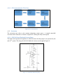
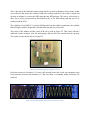
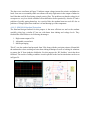
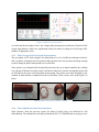
4TH QUARTER PROGRESS REPORT OF ICT R&D FUNDED PROJECT
Development of Flaw Diagnosis/ Dimensioning/ Prognostics Algorithms for
the Improvement of In-Country Aerospace Non-Destructive Testing (NDT)
Capabilities
PI: Dr Tariq Mairaj Rasool Khan
Co-PI: Dr Faisal Amir
Table of Contents
Table of Figures .............................................................................................................................. 3
Table of Tables ............................................................................................................................... 4
1
Introduction ............................................................................................................................. 5
2
Recruitment of Workforce for Fourth Quarter........................................................................ 5
2.1
3
Principal Project Progress ....................................................................................................... 7
3.1
Development of MATLAB functions from ET algorithms for the GUI .......................... 7
3.2
Development of MATLAB functions from UT algorithms for the GUI ......................... 8
3.3
Development of GUI for flaw detection and profiling software ...................................... 8
3.4
The ET GUI.................................................................................................................... 12
3.4.1
Magnitude Button ................................................................................................... 13
3.4.2
Histogram Button .................................................................................................... 13
3.4.3
Adaptive Thresholding Button................................................................................ 14
3.4.4
ROI Detection Button ............................................................................................. 15
3.4.5
Report Button .......................................................................................................... 16
3.5
4
Recruitment of Undergraduate Workforce ....................................................................... 5
The UT GUI ................................................................................................................... 16
3.5.1
Amplitude Scan (A-Scan) ....................................................................................... 17
3.5.2
B-Scan (Cross Sectional view Scan)....................................................................... 17
3.5.3
C-Scan (Top View) ................................................................................................. 18
3.5.4
FFT (Fast Fourier Transform)................................................................................. 18
3.5.5
STFT (Short Term Fourier Transform)................................................................... 19
3.6
Alpha Testing of GUI for flaw detection and profiling software ................................... 20
3.7
Hilbert Huang Transform Based Flaw Profiling Algorithms using Ultrasonic Testing 20
3.8
Generation of Historical Database ................................................................................. 21
Undergraduate Projects Progress .......................................................................................... 22
4.1
PC Based Eddy Current Testing System ........................................................................ 22
4.1.1
Previous Progress .................................................................................................... 22
4.1.2
Excitation ................................................................................................................ 23
4.1.3
Eddy Current Probe Design & Development.......................................................... 26
4.1.4
Phase Shift Detection & Demodulation .................................................................. 26
4.1.5
Demodulation using XOR Logic Gate .................................................................... 27
4.1.6
Filtering for required signal .................................................................................... 28
4.1.7
Data Acquisition & Signal Processing:................................................................... 28
4.2
ET Position sensor.......................................................................................................... 30
4.2.1
Previous Work/Approach........................................................................................ 31
4.2.2
Final Approach for ET Position Sensor .................................................................. 31
4.3
GWUT over WSNs ........................................................................................................ 34
4.3.1
Envelope detector circuit ........................................................................................ 34
4.3.2
Exciter circuit .......................................................................................................... 34
4.3.3
Wireless Sensor Networks ...................................................................................... 35
Appendix A ................................................................................................................................... 38
Table of Figures
Figure 1: Typical flow through figures for the ANDT FDS GUI ................................................... 9
Figure 2: Background image incorporated in every figure of the ANDT FDS GUI .................... 10
Figure 3: Text from previous figure as an example of inter-figure communication .................... 11
Figure 4: ET GUI Figure with buttons disabled until input files are selected .............................. 12
Figure 5: ET GUI figure showing Thresholded data .................................................................... 12
Figure 6: Image plot of Calibrated Magnitude ............................................................................. 13
Figure 7: Histogram of Image ....................................................................................................... 14
Figure 8: Image after Adaptive Thresholding Algorithm ............................................................. 15
Figure 9: Image with detected ROI's ............................................................................................ 15
Figure 10: Generated Report ......................................................................................................... 16
Figure 11: UT GUI Figure showing A Scans ............................................................................... 17
Figure 12: A-Scan ......................................................................................................................... 17
Figure 13: B-Scan ......................................................................................................................... 18
Figure 14: C-Scan ......................................................................................................................... 18
Figure 15: FFT Spectrum Plot ...................................................................................................... 19
Figure 16: STFT Spectrum Plot .................................................................................................... 19
Figure 17: STFT Time-Frequency Plot......................................................................................... 20
Figure 18: (a) is of Healthy location (b) is of Cracked Location of 3 mm dia. (c) is of Cracked
Location of 4 mm dia. and (d) is of Crack location of 5 mm dia.................................................. 21
Figure 19: Eddy Current Probes (hand wounded) ........................................................................ 22
Figure 20: ET Instrumentation ...................................................................................................... 23
Figure 21: OPA564 Based Howland pump .................................................................................. 23
Figure 22: OPA564 through-hole Adapter & Circuit ................................................................... 24
Figure 23: OPA564 Howland results (Resistive & Inductive loads) ............................................ 24
Figure 24: Inductive Load without Snubber ................................................................................. 25
Figure 25: Inductive Load with Snubber ...................................................................................... 26
Figure 26: Eddy Current Probes (machine wounded)................................................................... 26
Figure 27: Demodulated Output from Phase Locked Loop (PLL) ............................................... 27
Figure 28: Output of XOR Gate.................................................................................................... 27
Figure 29: Output of RC Low Pass Filter ..................................................................................... 28
Figure 30: Software Flowchart ..................................................................................................... 29
Figure 31: Data Logging on LabVIEW ........................................................................................ 29
Figure 32: Signal Processing using Filters on LabVIEW ............................................................. 30
Figure 33: Results of Filtering on LabVIEW ............................................................................... 30
Figure 34: GUI figure for the ET position sensor ......................................................................... 31
Figure 35: Real-time data acquisition displayed on command window ....................................... 32
Figure 36: Pointer Ballistics problem ........................................................................................... 32
Figure 37: Primary ET Position sensor GUI features and improvements .................................... 33
Figure 38: Graph of position vs time by ET position sensor, having some erroneous spikes ...... 34
Figure 39: Modulated Gaussian pulse........................................................................................... 35
Figure 40: Generation of modulated Gaussian pulse: Modulation approach ............................... 35
Figure 41: Console from Eclipse IDE showing output of java program ...................................... 37
Figure 42: Square waveform reproduced in Matlab ..................................................................... 37
Table of Tables
Table 1: Three Cracks Diameter Values ....................................................................................... 20
Table 2: Energy Distribution between 6 mm till 10 mm depth of Specimen ............................... 21
1 Introduction
The ICT R&D funded project, “Development of Flaw Diagnosis/ Dimensioning/ Prognostics
Algorithms for the Improvement of In-Country Aerospace Non-Destructive Testing (NDT)
Capabilities” started on April 1st, 2013. In this regard, an NDT Centre has been established at
Pakistan Navy Engineering College, National University of Sciences and Technology (PNECNUST). This document describes the activities that have been performed at the NDT Centre
during the fourth quarter of the project.
The activities for this quarter included re-recruitment of undergraduate workforce; Guided User
Interface (GUI) development for flaw detection software incorporating both ET and UT testing
methods; alpha testing of the GUI; and generation of historical database.
A website is also set up according to the directions of ICT R&D. The web site link is
http://ndt.pnec.nust.edu.pk/index.html. The web site contains details of different project
activities.
The details of project activities are as discussed in the subsequent sections.
2 Recruitment of Workforce for Fourth Quarter
Competitive and research oriented human resource is highly desirable for performing rapid
development activities. In this regard Under-Graduate (UG), Post-Graduate (PG), Research
Assistant (RA) and other support staff has been recruited. The UG students and staff have been
re-recruited for this quarter.
2.1 Recruitment of Undergraduate Workforce
Undergraduate recruitment for 06 positions was carried out instead of two positions as approved
in budget. A change of request form was raised giving justification of the change. The change
has been approved. According to the new plan 06 positions are filled on quarterly basis.
Short listing and selection of UG students depended upon their GPA, technical knowledge,
attitude, motivation, commitment for summers and final year project. The selected UG students
have been divided into two groups as follows:
For Fee Waiver:
1. Salar Bin Javaid
2. Taha Saeed Khan
For Stipend:
1. Talha Waqar
2. Summaya Abbas
3. Muhammad Mansoor
4. Sulaiman Rais
All the students listed above give 10+ hrs/ week to the project. Students are categorized into
different group-projects based on the various aerospace NDT techniques. The RA acts as the
principal supervisor and coordinator for these projects. The UG students availing tuition waiver
are acting as the group leaders. The UG group leaders are responsible for the tasks assigned to
the group by the PI, Co-PI and RA as well as other support tasks assigned from time to time.
Therefore, their committed time is greater as compared to other students.
The students listed above have been hired for fourth quarter only. Their continuous hiring is
dependent on their performance in the project. The leadership assignment may also be changed
based on performance and commitment to the project.
The groups may be further divided into sub-groups that will accomplish a specific task. These
groups may also be populated by students not taking any grant from the project, for instance,
they may be working for their FYP or involved voluntarily. Current groups or sub-groups
involved in different activities are as under:
1. Oscillator and Excitation for Eddy Current Testing (ET)
a. Sumayya Abbas
b. Salar Bin Javaid (Group Leader / Coordinator for ET)
2. Eddy Current Probe Design
a. Shayan Ahmed (FYP)
b. Mansoor Malik
3. Data Acquisition and Flaw Profiling for ET
a. Uzair Gilani (FYP)
b. Iqra Sajid (FYP)
4. Guided Wave Ultrasonic Testing (GWUT)
a. Taha Saeed Khan (Group Leader/ Coordinator for UT)
5. GWUT on WSN
a. Taha Saeed Khan
b. Umair Asif Shamsi
c. Sulaiman Rais
6. Position Sensor for ET with GUI
a. Talha Waqar Khan
b. Uzair Gillani
7. Development of GUI with RA
a. Salar bin Javed
b. Talha Waqar Khan
c. Taha Saeed Khan
For each group, there is at least one group activity and one group meeting/presentation scheduled
every week. The students are assigned aerospace NDT literature review, basic design projects
related to aerospace NDT data acquisition and NDT signal interpretation.
3 Principal Project Progress
Following were the technical milestones achieved in the preceding quarter:
1. Development of flaw detection software
a. Report generation module
2. Flaw Profiling algorithm development
a. Development of calibration curves
b. Development of Method based on neural networks
c. Development of method based on Bayesian technique known as SMC (sequential
Monte Carlo)
3. Generation of historical database
The technical milestones set for the reporting quarter are as follows:
1.
2.
3.
4.
GUI development for flaw detection and profiling software
Alpha testing of flaw detection and profiling software
User manual for flaw detection and profiling software, and its GUI
Generation of historical database
All of the milestones set for the fourth quarter are achieved except the incorporation of SMC
algorithm and some other methods in the GUI, such as the one based on Hilbert-Huang
Transform (HHT) which is developed for UT. The methods such as HHT are not originally
present in the project milestones, but are a productive addition. All methods will be incorporated
in the next release/version of GUI.
The development of stand-alone MATLAB functions (programs) from the flaw detection and
profiling algorithms for the GUI, the GUI itself, its alpha testing results and HHT based method
for UT are presented in the following sections:
3.1 Development of MATLAB functions from ET algorithms for the GUI
Following ET functions were developed in MATLAB software to realize the algorithms in the
form of software:
1.
2.
3.
4.
5.
6.
7.
ET_extract_data()
ET_calibrate()
ET_land_mark_elimination()
ET_Adaptive_Thresholding()
ET_morph_ops()
ET_roi_detection()
ET_feature_extraction()
8. ET_classification()
9. ET_report_generation()
These functions and their outputs are described briefly in section 3.4.
3.2 Development of MATLAB functions from UT algorithms for the GUI
Following UT functions were developed in MATLAB software to realize the algorithms in the
form of software:
1.
2.
3.
4.
5.
6.
7.
8.
UT_initialize()
UT_AScan()
UT_BScan()
UT_CScan()
UT_spctstft()
UT_emdn()
UT_hlhut()
UT_reportgen()
These functions and their outputs are described briefly in section 3.5.
3.3 Development of GUI for flaw detection and profiling software
A Graphical User Interface is necessary for any software to let the end users interact
conveniently without memorizing specific commands and following strict flow requirements.
Thus a well-designed GUI allows the software to assist the user in his/her work, without
disturbing the user’s focus with non-application specific details. In context of flaw detection and
profiling software, GUI should allow its user to identify faulty parts and quantize the flaw (if
present), without having significant knowledge of the signal processing algorithms being used.
The GUI is developed using ‘GUI Design Environment (GUIDE)’ tool of MATLAB software.
GUIDE allows developing the front panel or the User Interface (UI) interactively. This UI is
stored as a separate binary file called a ‘figure’ in MATLAB, with the extension ‘.fig’. It
basically contains an arrangement of different objects such as buttons, check-boxes, drop-down
lists, text-boxes, display axes, panel etc. and their properties. There may be many properties
related to an object in MATLAB depending upon its type. Some important groups of properties
that were set for different objects are described below:
1. Style/Appearance properties: which decide colors, font sizes etc. of the object
2. Base properties: which contain the handle tag and other important parameters of the
object
3. Control properties: which define the callback function and enable/disable status of the
object
4. Position properties: which define the size and relative position of the object
5. Data properties: which define the properties pertaining to the data or text the object
handles
The UI is programmed by the help of call-backs. Callbacks are technically function pointers,
which implement the logic to handle a particular event. Events are generated by user actions,
such as pressing a button or selecting a value out of the drop-down menu etc. Each object has its
own unique handle or pointer, by which it can be addressed. The UI is linked with a
corresponding ‘m-file’ by the help of handles and callbacks. A template containing call-back
functions is automatically generated by GUIDE, which can be populated for specific needs.
The GUI was named “Aerospace NDT Flaw Detection Software (ANDT FDS)”, and is
composed of five different figures. The ANDT FDS was developed as a set of figures instead of
a single figure to follow a modular approach: this allows re-usability and easy prototyping.
Moreover, a wizard like approach is adopted, which unburdens the user from doing routine
settings, and problems caused by forgetting to set important ones. Furthermore, each figure is
stand-alone as well i.e. it can also run directly. However, the first figure is a bit redundant as it is
only a welcome screen that may be omitted in latter versions. Each figure calls another figure,
until the user reaches the ET GUI or the UT GUI. Figure 1 depicts the flow the user can adopt
between figures.
A
Welcome Screen:
Press ‘Start’
NDT Method
Selection Screen
Target Area
Selection Screen
NDT Method?
Target Area?
1. Wings
2. Fuselage
ET
UT
ET GUI
UT GUI
3. Landing Gears
A
Figure 1: Typical flow through figures for the ANDT FDS GUI
Because of the modular approach, we can for instance, design a specific GUI for ET of Landing
Gears if future requirements compel us to do so.
Each figure contains a background axis, on which a common background image is displayed.
This background image contains the logos of PIA, ICTR&D, PNEC and NUST within top and
bottom strips. The title of the software is also evident on the top strip. Figure 2 shows this
background image. All other GUI objects including panels lie on front of this image except the
strips in every figure.
Figure 2: Background image incorporated in every figure of the ANDT FDS GUI
Each function has its own namespace. Therefore, any variables created or updated within a callback function are local to it. To communicate between call-backs, GUIDE creates and uses a
‘handles’ structure which is passed as a default parameter to every callback function. It primarily
contains handles to all objects on the current GUI figure. This structure is used for inter-callback
and inter-GUI communication in ANDT FDS by introducing new fields into it. Some important
fields introduced are listed below:
1. Handles for inter-GUI communication:
a. handles.igc.prev_fig_h: stores handle of previous figure, it is used to
delete previous figure when new figure is invoked.
b. handles.igc.ta_sel: communicates selection of target area to following
figures.
c. handles.igc.m_sel: communicates selection of NDT method to following
figures.
2. Handles for inter-callback communication in ET GUI:
a. handles.et.calib_filename: Stores calibration filename for ET
b. handles.et.calib_filepath: Stores calibration filepath for ET
c. handles.et.raw_filename: Stores raw filename for ET
d. handles.et.raw_filepath: Stores raw filepath for ET
e. handles.et.impedance: Stores raw impedance values returned by
ET_extract_data(), when ‘Load’ Button on the ET GUI is called. It is used
by different signal processing functions.
f. handles.et.impedance_mag: Stores
corresponding magnitudes for
handles.et.impedance
g. handles.et.Real_Component: Stores corresponding real components for
handles.et.impedance
h. handles.et.Imaginary_Component: Stores corresponding imaginary components
for handles.et.impedance
3. Handles for inter-callback communication in UT GUI:
a. handles.ut.calib_filename: Stores calibration filename for UT
b. handles.ut.calib_filepath: Stores calibration filepath for UT
c. handles.ut.raw_filename: Stores raw filename for UT
d. handles.ut.raw_filepath: Stores raw filepath for UT
e. handles.ut.A: Stores Amplitudes returned by UT_initialize() function
when ‘Load’ button is pressed on UT GUI. It is used by different signal
processing functions in various call-backs.
f. handles.ut.D: Stores distances corresponding to amplitudes in
handles.ut.A
Using the igc structure, the figures delete their parents and update their local variables with the
user selections made in previous figures. For instance, Figure 3 shows the Target Area selected
by user in the Target Area Select figure, which is displayed in Method Select figure as text in
Title bar.
Figure 3: Text from previous figure as an example of inter-figure communication
Both ET and UT GUI need data files to operate on. Therefore, all other buttons are disabled until
filenames or file paths for both calibration and data files are not selected. Figure 4 shows such a
scenario in ET GUI.
Figure 4: ET GUI Figure with buttons disabled until input files are selected
When files are loaded, ‘Load’ button activates but all others are still disabled. Pressing this
button calls functions which are needed before any other operation is done i.e. it initializes the
GUI, and enables all other buttons. This is true for both ET and UT GUI figures. When any other
button or command is passed, the GUI calls necessary functions listed in sections 3.1 and 3.2 in
predefined order. Among other requisite parameters, the GUI passes handles to display axis to
these functions, so that the functions can directly output results on the given axis. Such GUI
specific parameters are passed to the functions using variable argument inputs. This allows
debugging the functions when run stand-alone.
Following sections brief the ET and UT GUI figure commands in further detail.
3.4 The ET GUI
The ET GUI is developed for diagnosing and profiling flaws using Eddy current testing. Figure 5
shows the ET GUI figure showing thresholded data.
Figure 5: ET GUI figure showing Thresholded data
Important Buttons/Commands for the ET GUI are detailed as follows:
3.4.1 Magnitude Button
The magnitude button shows the image of calibrated impedance magnitude as shown in Figure 6.
The impedance has been calculated by extracting real and imaginary parts from the raw data of
particular area. The calibration has been done using two calibration parameters i.e. rotation
matrix and scaling factor. The image shown has comprises of various colors, ranges from blue to
red. The part which is in red means maximum deflection in that area from the probe and blue
color indicates no deflection. The deflection occurs due to the cracks, land marks and noise in the
signal. The colors in between blue and red indicates the strengths of different deflected signal.
Figure 6: Image plot of Calibrated Magnitude
3.4.2 Histogram Button
The histogram button displays the probability distribution of pixel values in an image in the form
of bar plot as shown in Figure 7. It bins the elements of image into 100 equally spaced containers
and returns the number of elements in each container and displays. Height of each rectangle
indicates the number of elements in the bin. It’s necessary to have an idea about how much
different amount of data present in the image before adaptive thresholding. The elimination
percentage of an image can be decided by visualizing the histogram of that image.
Figure 7: Histogram of Image
3.4.3 Adaptive Thresholding Button
Adaptive Thresholding button displays the processed image of particular area in an aircraft part
as shown in Figure 8. Adaptive thresholding is used to remove this ill influence which typically
takes a grayscale or color image as input and, in the simplest implementation, outputs a binary
image representing the segmentation. The areas in red are the possible effected regions in an
aircraft.
Figure 8: Image after Adaptive Thresholding Algorithm
3.4.4 ROI Detection Button
The ROI detection button shows the potential interested regions in the image as shown in Figure
9. The image formed after applying adaptive thresholding scheme which is in binary format.
Binary images may contain numerous imperfections. In particular, the binary regions produced
by thresholding are distorted by noise and texture. To find potential region of interest, a
morphological operation has to be performed. Morphological image processing pursues the goals
of removing these imperfections by accounting for the form and structure of the image.
Figure 9: Image with detected ROI's
3.4.5 Report Button
Report button displays the final report which gives adequate detail about the effected regions.
Generated report saves as a text format and place in the current folder. The first column
represents the location of potential regions in terms of rows and columns. The features such as
maximum reactance, maximum magnitude, phase at 200 kHz and phase at 100 kHz are extracted
from defined location. The values of the extracted features are placed in third column.
Classification of the ROI is done using heuristically defined rule and result is shown in the last
column i.e. either the detected ROI contains “DEFECT” or “NO DEFECT”.
Figure 10: Generated Report
3.5 The UT GUI
The UT GUI is developed for ultrasonic testing diagnostics part of the project. Diagnosis results
and their appearance are made user friendly, different push buttons are made for different
techniques to analyze ultrasonic result effectively, as shown in Figure 11.
Figure 11: UT GUI Figure showing A Scans
A brief overview of important buttons and their functionality for UT GUI follows:
3.5.1 Amplitude Scan (A-Scan)
Amplitude Scan is the plot between time and amplitude, where x-axis is time axis and y-axis is
amplitude. This is exactly the same plot which can be seen at the equipment screen at the time of
inspection. A-Scan is the base for all other processing of ultrasonic signal. Rough estimate can
be deduced from this plot.
Figure 12: A-Scan
3.5.2 B-Scan (Cross Sectional view Scan)
B-Scan is cross sectional view of the test specimen displayed graphically. B-Scans also termed
as brightness scan is obtained with the help for A-Scans at predetermined intervals. This is 2-D
type of plot in which we have linear distance on which scans are obtained displayed at X-Axis,
Y-Axis shows the depth of the test material and color shows the intensity of the pulse at specific
location.
Figure 13: B-Scan
3.5.3 C-Scan (Top View)
C-Scan is top view of the test specimen and it is top view thickness mapping of the material
which is obtained with the help of A-Scans. Thickness is calculated with the help of amplitude
scans and plotted accordingly. In C-Scan view we have dimensions (Length and Breadth) of the
actual piece on X-axis and Y-Axis and their thickness is along the Z-axis. With the help of CScan we can estimate the sub surface issues which are not visible with bared eye. Below mention
is sample C-Scan plot obtained using 25 location inspection results.
Figure 14: C-Scan
3.5.4 FFT (Fast Fourier Transform)
Fourier transform is one of the basic techniques used for signal characterization in frequency
domain. In this method multiplication has performed with the signal under observation and sine
and cosine. Sampling frequency is selected based on Shannon Frequency Theorem as transducer
used to carry out examination. In this frequency is at X-Axis (logarithm Scale) and Y-Axis refers
to amplitude. Figure 15 was obtained from one of healthy location of test specimen.
Figure 15: FFT Spectrum Plot
3.5.5 STFT (Short Term Fourier Transform)
Short Term Fourier Transform (STFT) shows three plots, first one is STFT spectrum, second is
Time Frequency plot at particular location and third is A-Scan [refer to section 1.1] for better
understanding of user. STFT Spectrum is three axes plot with time information in on X-Axis, YAxis represents frequency information and Z-Axis shows the amplitude of the signal. Figure 16
is the spectrum of healthy which is obtained using 6 point rectangular window; rectangular
window is most preferred for detection of discontinuity and abrupt changes.
Figure 16: STFT Spectrum Plot
Short Term Fourier Transform’s second plot is the Time-Frequency plot obtained at selected
location to observe the behavior of time and frequency at particular distance. User has been
given access to select point which gives Time-Frequency Plot similar to Figure 17
Figure 17: STFT Time-Frequency Plot
3.6 Alpha Testing of GUI for flaw detection and profiling software
Software Testing is a critical part of any software development. Alpha Testing is an initial part of
software testing, which is conducted by the developers and programmers to verify whether the
software under test is behaving as expected or not. The developers and programmers write a
‘User Manual’ which documents expected use and behaviour of the software. Alpha testing
ensures that the software functions according to the User Manual.
The GUI for flaw detection and profiling software has been tested by the development team, and
is working in accordance with the User Manual, which is attached as Appendix A.
3.7 Hilbert Huang Transform Based Flaw Profiling Algorithms using
Ultrasonic Testing
Flaw profiling using ultrasonic testing needs analysis of signal in time frequency domain due to
non-stationary nature of the signal i.e. there is an effect of time on signal frequency. Short term
Fourier Transform (STFT) was used to analyze raw signal which was obtained from test piece.
During analysis with the help of STFT different size of window was used to get better profile of
the crack. It was also assumed that signal was linear for certain duration whereas original signal
obtained from test piece was non-linear and non-stationary in nature. In order to analyze the
signal recent technique Hilbert Huang Transform has been used to get more accurate and precise
information about crack. Table 1 shows the crack diameters.
Table 1: Three Cracks Diameter Values
Content
Diameter
Crack 1
3 mm
Crack 2
4 mm
Crack 3
5 mm
Figure 18: (a) is of Healthy location (b) is of Cracked Location of 3 mm dia. (c) is of Cracked Location of 4 mm dia. and
(d) is of Crack location of 5 mm dia.
Figure 18 plots are the Hilbert Spectrum obtained from the test data and by analyzing the energy
distribution changes that occurs due to presence of crack. Figure 18 shows time frequency and
energy distribution of cracked and healthy location. It can easily be observed that there is no
energy between selected depth readings i.e. between 6 mm till 10 mm as there was no crack
whereas in rest of the figures we have some visible changes in energy distribution at and near to
cracked location. In order to profile the crack based on HHT spectrum plot, energy has been
added to get the relation between flaw size and energy values. Below mention is the table that
shows the summation of the points selected around cracked dimensions which clearly shows that
as the crack size increases more energy will be dissipated.
Table 2: Energy Distribution between 6 mm till 10 mm depth of Specimen
Content
Healthy
Location
Energy (6-10
mm depth)
0
Cracked Locations dia.
3 mm
4 mm
5 mm
0.0149
0.0168
0.0203
3.8 Generation of Historical Database
Through the generation of historical database the remaining useful life (RUL) of aircraft
structure can be predicted. This database would be used in damage progression/crack growth
studies for different structures/parts of the aircraft. The database would also show the
degradation progression in different components/specimens with respect to flight hours. The
knowledge of RUL would ensure aircraft safety as well as enable aircraft management agencies
to plan repair/replacement accordingly.
Thus development of historical database is a long and continuous process, which remained in
progress during the 4th quarter.
4 Undergraduate Projects Progress
Subsequent sections document the progress on different UG projects in the fourth quarter.
4.1 PC Based Eddy Current Testing System
4.1.1 Previous Progress
The undergrads started off with designing an alternating current source but with constant peak
value. The few designs tried were reported in the 3rd quarter report. The IC OPA564 that was
ordered from abroad, for the constant current source. It was obtained in SMD form and hence
practical testing could not be done immediately after the procurement.
Probe design and development was also carried out using the ‘Analytical Approach’ that
incorporated graphs and constants for the physical parameters of the copper wire used. Three
different probes were developed with different inductances and the one with 106uH was
finalized. It did not give accurate results due to the fact that it was hand wounded. These can be
seen below in Figure 19.
Figure 19: Eddy Current Probes (hand wounded)
The third most important hardware part of the project is the demodulation stage for demodulating
the signal received from the eddy current probe. For this purpose a ‘Phase Locked Loop’ which
is a phase sensitive detector was chosen and some work was done in order to use it to detect a
phase change in the signal offered by the eddy current probe.
4.1.1.1 ET Instrumentation Flowchart
Figure 20: ET Instrumentation
4.1.2 Excitation
The excitation part refers to the constant alternating current source. A smooth sinusoidal
waveform with current above 500mA is required for exciting the eddy current probe.
4.1.2.1 OPA564 Based Howland Current Pump
The high current operational amplifier IC OPA564 chosen for this purpose was procured by the
end of 3rd quarter. The design for OPA564 finalized is shown on the right in Figure 21.
Figure 21: OPA564 Based Howland pump
This is known as the Howland current pump which was tried on hardware and accurate results
were achieved. But before the students could start working with the IC they had to design and
develop an adapter to convert the SMD package into DIP package. This was a critical task as
there was a power pad provided at the bottom of the IC for heat sinking and that was to be
soldered with the PCB.
The soldering of an SMD IC is already difficult and with this added requirement, the students
had to design a suitable design that was both sufficient and easy to develop.
The results of the adapter and the circuit PCB can be seen in Figure 22. This circuit offered a
sufficient current at output. Also the load changes did not affect the current from the op-amp.
The results are also shown below in Figure 23.
Figure 22: OPA564 through-hole Adapter & Circuit
Precision resistors of tolerance 0.1% were still awaited hence this circuit was designed using
local precision resistors with tolerance 1%. But even then, a reasonably stable waveform was
achieved.
Figure 23: OPA564 Howland results (Resistive & Inductive loads)
The above two waveforms in Figure 23 indicate output voltage/current for resistive and inductive
loads. One can see reasonably stable waveforms with only slight noise in the output of inductive
load. But that could be fixed using a simple passive filter. The problem was that the voltage level
at output was very low which would have been difficult to detect practically. Also the IC had a
problem of quickly getting heated up. As a result of this, the students burnt two such ICs due to
problem of voltage spikes from inductor/ coil and heating up of the component.
4.1.2.2 OPA548 & Howland Protection
The Howland design finalized for this purpose is the most efficient one and so the students
carefully picked up a similar IC but one with better heat sinking and voltage levels. They
finalized the OPA548 due to its following advantages:
1. High current output of 5A
2. Adjustable current limit
3. Mosfet packaging
This IC was also ordered and procured from USA along with the precision resistors. Meanwhile
the students have been working on better heat sinking techniques as well as looking for solutions
to protect the IC from inductive kickbacks. For this purpose the ‘RC Snubber’ circuit has been
finalized. The results of adding a snubber circuit in parallel to the load on simulation can be seen
in Figure 24.
Figure 24: Inductive Load without Snubber
Figure 25: Inductive Load with Snubber
As seen from the two figures above, the voltage spikes during turn on and turn off period of the
circuit using inductive load were significantly reduced in terms of voltage level by using an RC
snubber of appropriate value.
4.1.3 Eddy Current Probe Design & Development
The next phase of ET Probe design is the fabrication of a coil of sufficient inductance which is
able to produce a magnetic field to generate eddy currents in the test specimen and large enough
to show change in phase when passed over a crack/flaw.
Some probes were designed and developed but because they were hand wounded, the winding
was coming off & hence accurate results could not be achieved even after exciting the probe with
an efficient circuit such as the Howland current pump. The probes were then designed by the
students & then machine wounded from the local market. These can be seen in the Figure 26
below.
Figure 26: Eddy Current Probes (machine wounded)
4.1.4 Phase Shift Detection & Demodulation
With reference from the previous report, the Phase Locked Loop was finalized for FM
demodulation. The students have already purchased the PLL IC CD4046B and are trying to use it
as a demodulator. Initially the working of the IC was successfully verified in its most simple
design by checking the operation of the built-in Voltage Controlled Oscillator (VCO) of the IC.
To start with, a self-generated FM signal was used to test the PLL as a demodulator. The FM
signal was designed on MATLAB and tested on hardware. The result of which is shown in
Figure 27. Later when actual results were obtained from the eddy current probe, the signal was
passed on to the PLL and it was working just fine. Only problem was that the sensitivity of the
PLL could not detect the feeble phase shift offered by the eddy current probe under use.
Figure 27: Demodulated Output from Phase Locked Loop (PLL)
4.1.5 Demodulation using XOR Logic Gate
As a result the students had to find some other means of detecting the phase shift obtained
between the two signals, input and output. The XOR gate was finalized which is a logic gate that
produces a high output only when one of the inputs is high. In our case the input and output
signals are 180 degrees out of phase Hence the XOR produces high output for every part of the
cycle as the inputs are different except at zero crossing and its results can be seen below in
Figure 28.
Figure 28: Output of XOR Gate
The result of this XOR was a square wave whose pulse width changed when the probe was
moved from air close to the test specimen and then over the crack and non-crack.
4.1.6 Filtering for required signal
The next step was to filter this output to get a dc signal whose voltage level would vary as the
phase would change.
There are two filtering techniques available:
1. Passive RC filter
2. Active filter
Initially the students designed and developed a passive RC circuit. The results of which can be
seen below in Figure 29.
Figure 29: Output of RC Low Pass Filter
The output waveform shown in blue color was observed at a time scale of 1s. The two voltage
levels indicate the voltages in air and near test specimen whereas the small spikes seen at the
bottom indicate the presence of crack.
As clear from the above waveform that there was a lot of noise seen in the dc output which can
give false alarm of a crack in from of voltage spikes. Hence the students are working on the
active filter approach in order to minimize the noise at output and to increase the voltage level of
the signal.
4.1.7 Data Acquisition & Signal Processing:
Meanwhile, the students have also started working on the software side of the project as well.
The modulated signal has to be interfaced to the PC using a Data Acquisition (DAQ) card which
has also been procured.
The signal from the EC probe will be interfaced to the PC and plotted on software like
LABVIEW, which is a graphical programming language which will be used for real time data
acquisition and display plus analysis.
Following flowchart shows the functions that are to be carried out on software as seen in Figure
30.
Figure 30: Software Flowchart
Programming was done on software in order to learn data logging techniques on LabVIEW
software and how to interface it with the DAQ card see Figure 31.
Figure 31: Data Logging on LabVIEW
Similarly, filtering was also done on software by introducing noise randomly in a given signal.
Its programming was also done and the results can be seen below in Figure 32.
Figure 32: Signal Processing using Filters on LabVIEW
Original Signal
Self-Induced Noise
Filtered Signal
Figure 33: Results of Filtering on LabVIEW
The above procedure was only done for learning purposes. Results are as seen above in Figure
33. The demodulated signal is still being worked upon for reduction of noise and amplification to
get acceptable voltage level.
The students are currently working on the demodulation stage of the project and then will be
moving on to the software side in the upcoming month.
4.2 ET Position sensor
Manual scanning methods give reading with respect to time. Due to non-uniform speed the
accuracy decreases because in eddy current testing we want coordinates of the position moved by
the probe versus eddy current signal instead of time. Therefore, ET Position Sensor project was
initiated to easily determine the exact position of the crack/flaw.
4.2.1 Previous Work/Approach
PIC microcontroller was sought to be used having serial interface with PC. But it was a
mechanical platform: a ball mouse recording the increment in the mouse wheel for position
sensing as the ball moved x and y wheels of the internal circuitry.
It posed following problems: Complex external interfacing and data acquisition at a very fast rate
was very difficult. Moreover, its accuracy could be disturbed by mechanical factors such as ball
slip or backlash.
4.2.2 Final Approach for ET Position Sensor
Software based approach was adopted. This involves capturing the position increment sent by
mouse to the operating system for cursor movement. MATLAB based GUI was implemented
using ‘GUIDE’ tool. In this approach, Mouse position changes are taken as probe displacements,
where probe will be attached to the mouse assembly. The GUI’s axis that acts as a Cartesian
plane is shown in Figure 34.
Figure 34: GUI figure for the ET position sensor
4.2.2.1 Features implemented and further improvements
1. Real-time acquisition of data and display on command window was implemented, which lists
x-y axis position and time instantaneously. Figure 35 shows real-time data acquired from
mouse.
Figure 35: Real-time data acquisition displayed on command window
2. Pointer ballistics problem was also solved. Pointer Ballistics refers to the error caused due to
difference in mouse and cursor velocities with different mouse accelerations. Actually a nonlinear relationship is maintained by the operating system between the two velocities to ease
pointer perception for the user. This is shown in Figure 36. But to make this relationship
linear, a registry setting relating to mouse cursors is modified by the software.
Figure 36: Pointer Ballistics problem
3. To delimit the position sensor from pointer’s screen limitation, java.awt.robot function was
used to make pointer come back to origin of screen as it approached the end of the screen,
retaining its reading. In this way it continues the reading as it can be moved multiple time
across the screen taking readings so that there is no effect on the movement of physical
mouse structure placed on the plate.
4. Screen size was set to ‘full screen’ for easy calibration and avoiding to get out of the
specified path.
Figure 37 further illustrates various features of ET position sensor GUI:
Figure 37: Primary ET Position sensor GUI features and improvements
4.2.2.2 Future tasks
Though ET position sensor is operating successfully some minor issues related to the working of
the mouse near the screen limit exists. If the mouse is moved very fast then it sometimes gets out
of the screen limit and java.robot function can’t detect if it has moved out of the limit. When this
happens the pointer gets struck on the extreme edge of the screen and can’t move in the direction
of motion, yet if moved in other direction it gets detected and comes back to origin. Figure 38
shows the graph plotted for distance covered by mouse against time, which has some spikes due
to the issue discussed above. This problem is being resolved.
Figure 38: Graph of position vs time by ET position sensor, having some erroneous spikes
4.3 GWUT over WSNs
4.3.1 Envelope detector circuit
Up till third phase, we were working with only 300 kHz PZTs. In fourth phase, we imported
some new PZTs which are larger, thicker and more robust with lower resonant frequency, i.e.
200 kHz. First, we confirmed the resonant frequency by exciting the PZT in series with a resistor
and noting the voltages across it. A dip in voltage near 200 kHz indicated series resonance within
PZT as expected in Radial mode. We continued our work with those new low cost PZTs and
found some good results. Due to change in frequency (now working at lower frequencies) we
faced problems with envelope detector that was designed for 300 kHz. So we first redesign it
mathematically for variable frequencies and then check it practically. We also derived a
mathematical equation for its RC based filter for Gaussian signal.
4.3.2 Exciter circuit
After redesigning of envelope detector, we moved towards the designing of the exciter
circuit. The exciter circuit has to replace the function generator being used to excite the PZTs. A
modulated Gaussian pulse is used to excite the PZT at its resonant frequency, see Figure 39.
Figure 39: Modulated Gaussian pulse
Presently, we are concentrating on designing exciter circuit using modulation approach: A
Gaussian pulse will be generated using Zigbee motes’ integrated Digital to Analog Converter
(DAC), which will then be multiplied with an oscillator circuit using AD633 multiplier IC. This
is because the on-board DAC is incapable of generating signals of the order of hundreds of kHz;
however, it can easily generate Gaussian pulses, which can be re-programmed easily as well.
AD633 has been theoretically and practically tested for multiple frequencies. This approach is
represented in Figure 40.
Figure 40: Generation of modulated Gaussian pulse: Modulation approach
4.3.3 Wireless Sensor Networks
After completion of prior objectives discussed in previous reports, we commenced the task of
increasing the data sampling rate to 200 kilo samples per second. In consideration of Aliasing
and ADC sampling issues, we did not jump to increasing the sampling rate form 5 kHz to 200
kHz directly but decided to do this in discrete steps (increasing it 2 times, then 4 times and so on
up till 200 kHz).
Data sampled by this technique will be transmitted to a base station mote, however, before
moving onto this task the team decided to test ADC operations in WSN so that any sampling
issues with ADCs in motes could be appropriately addressed. The main idea was to isolate ADC
operations in motes from Wireless transmission of data from one mote to another. Therefore, we
decided to communicate data from a single mote serially to a computer, this allowed us to
address issues with ADC sampling and the amendments done previously in our Tiny OS
program.
At the time we succeeded in:
1.
2.
3.
4.
Increasing the sampling rate to 10 kHz
Retrieving a square wave signal serially from a mote
Extracting information bits from a Tiny OS data package through a java program
Reproducing the square wave signal in MATLAB
Currently we are working to further increase the sampling rate to 200 kHz.
4.3.3.1 Java program for extracting information bits
A WSN data package in Tiny OS contains the following bits:
1.
2.
3.
4.
Header
Metadata
Data bits (Information)
Footer
Except ‘data bits’ all other bits were found to be superfluous for reproducing a signal from a
zigbee mote on a base station, these superfluous bits are however mandatory for data
transmission and cannot be deleted from a package. In order to obtain only the information bits a
program was written in java. By considering the fact that a total of 20 bits are transferred in each
packed at a fixed offset from the current package’s starting point an algorithm was devised and
implemented in java. The program was developed and tested in Eclipse IDE. Figure 41 shows
the program’s output.
The program processes serial data in the following sequence:
1.
2.
3.
4.
5.
6.
Obtains the log file where data was previously logged
Converts data in file from ASCII code to Hexadecimal form
Extracts information bits from a series of packets
Formats data bits into groups of four hexadecimal codes
Converts the formatted data into decimal form for plotting in MATLAB
Creates (if required) and logs data into a file.
Figure 41: Console from Eclipse IDE showing output of java program
During final testing a square wave, generated using a function generator, was fed into a WSN
mote. That mote was connected to a computer USB port and data was logged into a file.
Information bits were extracted from the logged file through the program mentioned earlier .The
obtained data bits were then used to plot a waveform in MATLAB as illustrated below in Figure
42.
Figure 42: Square waveform reproduced in Matlab
Appendix A
Aerospace NDT GUI v1.1
User Manual
1. Run the code on MATLAB. The Aerospace NDT GUI should appear on screen. The first
window that will appear is the welcome screen:
2. Click start to proceed. Clicking start leads to a window which allows the selection of a
target area of the aeroframe, namely, the Fuselage, Wings or Landing Gear.
3. Upon selection of the target area the following window pops up, prompting the user to
select between the method of Aerospace NDT through which the data has been acquired:
4. Clicking either one of the options leads to a unique GUI designed and coded for
processing particular data. Depending on what the user clicks the following windows will
appear:
a. Eddy Current
As evident from the figure shown above the calibration file & raw data directory need to be
loaded
in
order
to
activate
the
Eddy
Current
GUI.
Clicking on the Select Calibration File button opens up a window which allows the user to
select a “.dat” file.
Select the file and click open.
Next click the Select Raw Data Directory button. Another window will appear from which the
user can select the folder to which the data will be directed.
Click Select Folder.
After the file and the folder have been selected the user can click the Load button to load the
selected data and enable the other buttons. The user can now access the various buttons present.
The impedance plot of raw data is displayed by default.
The buttons and there functions are as stated:
i.
Magnitude button
The magnitude button shows the image of calibrated impedance magnitude. The image
comprises of various colors, ranged from blue to red. Red means maximum deflection in
the area from the probe and blue indicates no deflection. Deflection occurs due to the
cracks, land marks and noise in the signal. The colors in between blue and red indicates
the strengths of different deflected signals.
ii.
Histogram button
The histogram button displays the probability distribution of pixel values in an image in
the form of a bar plot. It bins the elements of image into 100 equally spaced containers
and returns the number of elements in each container and displays. The height of each
rectangle indicates the number of elements in the bin. For finding the region of interest,
it’s essential to have an idea of the different data present.
iii.
Adaptive Thresholding button
The adaptive thresholding button displays the processed image of particular area in an
aircraft part. Adaptive thresholding is used to remove the ill influence which typically
takes a grayscale or color image as input and, in the simplest implementation, outputs
a binary image representing the segmentation. The area in red is the possible effected
region in an aircraft.
iv.
ROI Detection button
The ROI detection button shows the potential interested regions in the image. To find
potential region of interest, a morphological operation has to be performed.
Morphological image processing pursues the goals of removing these imperfections by
accounting for the form and structure of the image.
v.
Report button
The report button displays the final report which gives adequate detail about the effected
regions. Generated report saves as a text format and place in the current folder. The first
column represents the location of potential regions in terms of rows and columns. The
features such as maximum reactance, maximum magnitude, phase at 200 kHz and phase
at 100 kHz are extracted from defined location. The values of the extracted features are
placed in third column. Classification of the ROI is done using heuristically defined rule
and result is shown in the last column i.e. either the detected ROI contains “DEFECT” or
“NO DEFECT”.
b. Ultrasonic
As evident from the figure shown above the calibration file & raw data directory need to be
loaded
in
order
to
activate
the
Eddy
Current
GUI.
Clicking on the Select Calibration File button opens up a window which allows the user to
select a “.dat” file.
Select the file and click open.
Next click the Select Raw Data Directory button. Another window will appear from which the
user can select the folder to which the data will be directed.
Click Select Folder.
After the file and the folder have been selected the user can click the Load button to load the
selected data and enable the other buttons. An axes is displayed by default.
The buttons and there functions are as stated:
i.
A Scan
The Amplitude Scan button gives the plot between time and amplitude. This is exactly the
same plot which can be seen at the equipment screen at the time of inspection. A-Scan is the
basis for all other processing of ultrasonic signals.
ii.
C Scan button
The C Scan button gives the top view of the test specimen and it is top view thickness
mapping of the material which is obtained with the help of A Scans. With the help of CScan the user can estimate the sub surface issues which are not easily visible.