Download ETACE Virtual Appliance User Manual

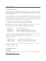
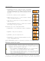
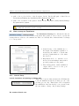
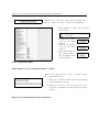
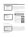
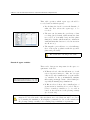
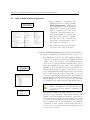
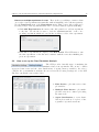
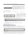
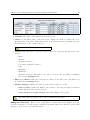
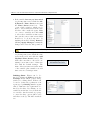
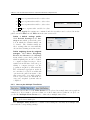
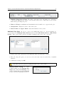
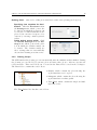
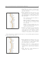
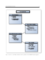
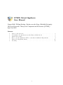
ETACE Virtual Appliance
User Manual
Gregor Böhl, Philipp Harting, Sander van der Hoog, Bielefeld University
Chair for Economic Theory and Computational Economics (ETACE)
April 16, 2015
Contents
1
2
3
4
5
6
Purpose and Overview . . . . . . . . . . . . . . . . . . . . . . . . . . . .
Programmes, Documentation and the Eurace@Unibi Model . . . . . . .
Quick Starter Guide . . . . . . . . . . . . . . . . . . . . . . . . . . . . .
How to use the Simulation GUI for customized Simulation Experiments
Flame Modeling Environment . . . . . . . . . . . . . . . . . . . . . . . .
Licensing . . . . . . . . . . . . . . . . . . . . . . . . . . . . . . . . . . .
1
.
.
.
.
.
.
.
.
.
.
.
.
.
.
.
.
.
.
.
.
.
.
.
.
.
.
.
.
.
.
2
2
2
4
21
23
1 Purpose and Overview
1
2
Purpose and Overview
This User Manual for the ETACE Virtual Appliance describes how to conduct economic analyses with the Eurace@Unibi model using the programmes available on the VA and its respective
tools, with regard to the general workflow of the Flexible Large-scale Agent-based Modelling
Environment (FLAME1 ).
The virtual appliance has been created at ETACE, the Chair for Economic Theory and
Computational Economics, at Bielefeld University. The intention behind this software collection
is to make every step related to the initialization, execution, modification and analysis of the
Eurace@Unibi agent-based simulation model as easy as possible. We hence address here the
issue of reproducibility of simulation-based research (Stodden, 2010).
2
Programmes, Documentation and the Eurace@Unibi Model
This software package is based on the SliTaz distribution of free software, that includes the
Linux kernel. The coresponding documentation is included in the software.
Programs provided in the Virtual Appliance (including their dependencies):
Xparser GUI
GNU GCC compiler
Flame Editor
Population GUI
Simulation GUI
:
:
:
:
:
Parser for FLAME models.
C compiler for model + framework code.
Generate model.xml file, XML description of model.
Generates initialization files, population description.
Settings for simulation experiments and data analysis.
Apart from standard dependencies such as GNU GCC, the relevant documentation to these
programmes can be found in the Documentation folder on the Desktop.
The following versions of the Eurace@Unibi model are included and can be found on the
Models folder on the Desktop:
Dawid
Dawid
Dawid
Dawid
et al., 2011
and Gemkow, 2013
et al., 2014b
et al., 2014a
:
:
:
:
full source code of Eurace@Unibi 1.0
main, model.xml, 0.pop & 0.xml for replication
full source code of the model used for the paper
full source code of the model used for the paper
For the following papers, a pre-configured ready-to-run experiment can be found in the
Preconfigured Experiments folder:
Dawid et al., 2014a
3
: XXX
Quick Starter Guide
The Desktop
After launching, you should see the desktop of the VA. The desktop contains folders and program
launchers. The folders are
1
http://www.flame.ac.uk/
3 Quick Starter Guide
3
• Documentation; this folder contains the licenses of the ETACE
Virtual Appliance, as well as manuals for GUIs and applications
used in the VA. Furthermore, it contains a description of the Eurace@Unibi model together with several research papers based on
the model.
• src; this folder contains source files of applications.
• Models; this folder hosts source code and executables of different
versions of the Eurace@Unibi model.
• exper; this is an empty folder for storing new simulation experiments of the user.
• Preconfigured Experiments; this folder contains ready-to-run simulation setups for exact paper replication.
The launchers can be used to launch different GUIs:
• PopulationGUI; to create an initial state as input of a simulation.
• AgentGUI; to change the model structure.
• xparserGUI; to parse and compile the model.
• SimulationGUI; for setting up and starting simulations as well as
post-processing simulation data.
Only the SimulationGUI is required for replicating the experiments of the paper.
Performance and the Linux system
The virtual appliance is set up with a minimum performance configuration. You can
increase the performance of the VA especially by increasing the number of processors
and the size of the allocated memory. However, the performance is limited by the
configuration of the host system. To change these:
• Enable hardware virtualization support in your own system’s BIOS to
run in multi-core mode (normally under menu ”CPU” in BIOS).
• In the settings of the virtual machine itself (i.e. in the client fi Oracle’s VirtualBox but not inside this virtual appliance), you can change the number of
assigned CPU cores and RAM memory.
To get root access in a terminal, type su with password root. The Super User is likewise
root with password root. All the relevant files have been placed on the Desktop (/home/eurace/
4 How to use the Simulation GUI for customized Simulation Experiments
4
Desktop), whereas additional libraries (Libmboard, R, Python, GSL) have been installed directly
into the system.
4
How to use the Simulation GUI for customized Simulation Experiments
The SimulationGUI has been developed to have an all-in-one user interface for setting up,
running, and analyzing simulations of models implemented in FLAME.
The general design of the GUI acknowledges that setting up and analyzing simulation experiments are two separated tasks, the first done before the simulation and the second after
the simulations have finished. These tasks are also separated in the GUI, which is achieved by
providing two separated tabs, one for the simulation settings and another for the post-processing
of the data. The Simulation GUI helps you to perform the following steps:
Design of the Computational Experiment
1. Setting the environment constants (model parameters)
2. Selection of data storage options: agents to store, at which frequency (every iteration,
every month,...)
3. Running a set of batch runs
4. Launching the simulation
5. After the simulation has finished and all data has been produced, the final stage is the
data analysis stage. For this, we again make use of the Simulation & Analysis GUI.
4.1
Getting Started: Define the Work Space and Enter basic Settings
The GUI works with a workspace environment. This means there is a folder in the file system
of the VA that is defined by the user as the location where all files related to a simulation
experiment are located.
How to set the Workspace There are two possibilities to set the current workspace:
1. Set the workspace immediately after launching the GUI: a file browser opens after launching the GUI which can be used to load an existing workspace or to create a new workspace.
• Load an existing workspace: use the file browser to browse to the top level folder of
the workspace. Click Open to load the settings. The GUI reads the saved settings
of the workspace and opens the main dialog window.
• Create a new workspace: use the file browser to browse to a location in the file
system where the new workspace should be created. Use the new folder button to
create and name the workspace. In the following, the user has to set some basic
settings manually. Use the file browsers to set the path to
–
–
–
–
the model xml file eurace model.xml
the main executable (main)
the initial start state (0.xml)
The top level folder of the R scripts. The default is:
4 How to use the Simulation GUI for customized Simulation Experiments
5
/home/eurace/Desktop/src/JavaGUI/src/Data Analysis GUI Serial.
– The executable of the xparser. The default is:
/home/eurace/Desktop/src/xparser-0.17.1/xparser.
2. Use the Experiment menu of the main menu bar and click Load to open an existing
workspace. Use the file browser to browse to the top level folder of the workspace and
load the workspace by clicking Open. To create a new workspace, click New. Use the file
browser to browse to the location where the new workspace should be created. The new
workspace is initialized with the current settings.
Save the current state of the workspace The current state of the workspace can be saved by
using the Save item of the Experiment menu. The previously saved settings are overwritten.
Alternatively, one can create a new workspace by using the Save as item of the Experiment
menu. In this case, one gets a new branch of the workspace without overwriting the old settings.
Importing and Exporting special configurations There can be the situation that the user wants
to flexibly use different settings as e.g. plotting settings without switching between workspaces.
For this case, the user can use the import and export feature of the GUI. Use the Import/Export item of the Experiment menu to export and import settings without branching the
workspaces. The settings which can be imported/exported are
• Plotting Settings: Exporting and importing the settings related to the data analysis.
This is to use different plotting profiles.
– Exporting: Use the file browser to define a location to which the plotting settings are
exported. The GUI writes a xml file with the currently used plotting settings. The
name of the file has to be specified by the user.
– Importing: Use the file browser to browse to the export location. Select and import
the xml file in which the plotting settings have been exported.
• Parameter Settings: Export and import parameter settings in order to switch between
different parametrizations of the model.
– Exporting: Use the file browser to define a location to which the parameter settings
are exported. The GUI writes a xml file with currently used parametrization of the
model. The name of the file has to be specified by the user.
– Importing: Use the file browser to browse to the export location. Select and import
the xml file in which the parameter settings have been exported.
Setting the required file paths manually When creating a new workspace from scratch, the
user is automatically asked to set the correct path to several file resources required by the GUI.
However, these paths can also be set manually. It should be noted that these path are mandatory
and have to be set correctly before setting up an experiment.
Use the Set Paths item of the Settings menu to check or change paths used for the
simulation. The paths to be set are
• path to the eurace model.xml file.
• path to the main executable.
• path to the 0.xml file.
4 How to use the Simulation GUI for customized Simulation Experiments
6
• path to the top level folder of the R scripts. In the VA the full path of this folder is
/home/eurace/Desktop/src/JavaGUI/src/Data Analysis GUI Serial/.
• path to the executable of the xparser. In the VA the full path is /home/eurace/Desktop/
src/xparser-0.17.1/xparser.
For the pre-configured experiments in ./Preconfigured Experiments/, all
paths have already been set correctly.
4.2
How to setup an Experiment
The Simulation Settings tab, which is the first tab
on the main dialog window, can be used to specify the
settings that are related to the simulations. There are basically three different kinds of settings
to be can specified:
1. General setup of the simulations, i.e.
the length of the simulation (number of
iterations), the number of batch runs
and the parametrization of the simulated model.
2. Experiment mode, i.e. whether or not
the model is run multiple times with a
specified parameter being varied.
3. Data management; which simulation
output will be stored for the postsimulation analysis.
4.2.1
General Setup
Launch simulations and plotting or plotting only
These radio buttons define whether the GUI launches
both, the simulations and the plotting process or the
plotting process only. This feature can be helpful if
the simulation data has already been generated and
the user wants to change only plotting settings.
Set number of batch runs
4 How to use the Simulation GUI for customized Simulation Experiments
7
Enter the number of batch runs. For each parameter
value of the experiment, the GUI launches the corresponding number of simulations. The runs only differ
by the random seed used.
Entering new values in any text field must always be confirmed by hitting enter.
Note on random seeds: The random seed is a parameter (model constant) in the model.xml
file called RND SEED that needs to be initialized (or else defaults to zero). This allows us to
include the value of the random seed in the 0.xml file, and then use it as an input into the simulation. This way, for all runs we use a different random seed, and still have full reproduceability
of the simulation results, because the value of the seed is stored in the initialization files.
Set number of iterations
Enter the number of iterations. Each simulation run
is executed for the indicated number of iterations. In
the Eurace@Unibi model, one iteration corresponds to
one day. Considering only working days, 5 iterations
constitute a week, 20 iterations a month and 240 iterations a year. A good starting point for a standard
experiment is 5000 iterations, which corresponds to 20
years.
Set number of process threads
This pull-down menu can be used to set the number
of simulation processes. This is helpful to reduce the
simulation wall-time of an experiment.
It is recommended to execute simulations in multiple process threads but to limit
the number of threads to the number of cores with which the VA is configured.
Change the parametrization of the model
4 How to use the Simulation GUI for customized Simulation Experiments
8
This button opens a new dialog window which can be
used to change the value of any model parameter.
• New parameter values can be entered
in the table.
Hit return after entering a
new value.
• Confirm the changes
and close the dialog
window.
• Discard the changes
and close the dialog
window.
• Reset all changes to
the default values of
the experiment saved
in the 0.xml file.
4.2.2
Experiment Mode
Select whether or not a model parameter is varied
These radio buttons can be used to switch between
two experiment modes:
1. Run only one Batch: run a batch only with the
current parameter setup.
2. Parameter Variation with one Parameter : a selected model parameter is varied among specified
values
Select the model parameter for the experiment
4 How to use the Simulation GUI for customized Simulation Experiments
9
Clicking Edit Parameter 1 opens a dialog window in
which the user can select the parameter to be varied
in the experiment as well as can define the parameter
values used in the experiment. This button is only
active if the radio button Parameter Variation with
one Parameter is selected.
• Scroll through the list of parameters and
choose the parameter for the experiment by
clicking on that parameter.
Clicking the right mouse button
orders the list alphabetically.
• Enter one value or multiple, by comma separated
values in the text field.
Confirm by clicking Add or
return.
• Select one or more values
and click remove to remove
these values from the list.
• Click OK to confirm all
changes and close the dialog window.
• Discard the changes and
close the dialog window.
4.2.3
Data management
Compress or decompress the databases
These radio buttons can be used to define whether or
not the databases should be compressed after finishing
all jobs. Depending on the storage settings, compressing databases can save hard disk space. These radio
buttons can be used in combination with the Do not
run radio button to compress and decompress data
bases without running the simulations again.
Data recording of agents
4 How to use the Simulation GUI for customized Simulation Experiments
10
This table specifies which agent type should be
recorded and at which frequency.
• By checking the check boxes in the Record column, the user selects the agent type to be
recorded.
• The user can determine the periodicity of data
recording (20 by default, which means the data
is recorded on a monthly base) and the phase
shift (0 by default, which means in combination
with period 20 that data is recorded at iteration
20, 40, 60 etc.).
• The snapshot option allows to record a full snapshot of the agent population with the specified
phase and periodicity.
Hit return after entering a new value.
Record all agent variables
These radio buttons are important for the space requirement of the VA.
• If Yes is selected, then the full memory of each
selected agent is written to disk. As one typically needs only a small subset of agent’s memory variables for the post-simulation analysis,
this setting can imply a waste of hard disk space
especially if running large simulations.
• If No is selected, then only a small subset of
agents’ memory variables are recorded. The selection of memory variables to be recorded is
based on the selection for the plotting settings
(see Section 4.4).
If choosing option No, only the variables that have been selected in the plotting settings are recorded. Be aware of the fact that non-recorded data can only be recovered
by re-running the simulation. It is highly recommended to choose the variables in
the plotting settings carefully before starting larger simulation experiments.
4 How to use the Simulation GUI for customized Simulation Experiments
4.3
11
How to build and Run experiments
• Before starting a simulation, the
simulation has to be built by clicking
Build Experiment. This means
the configuration of the experiment,
which has been entered through the
GUI, is translated into files (*.sh,
*.xml and *.txt files) which can be
read by the simulator to run the simulations, the R software to analyze
the data and by the operating system for file operations and to control
the sequence of activities.
• The GUI writes these scripts in the
top level folder of the work space.
• Clicking Run Experiment launches the actual simulation
experiment. A simulation experiment is a two step process:
1. The simulation of the model. The simulator (main executable) is executed and writes the simulation data as
output to file. The progress of the simulation is indicated by a progress bar which automatically pops up
when the simulation is being started. For writing the
simulation data, the GUI creates a folder with a specific hierarchy in the workspace with its as top level
folder. Each simulation run is written in a specific sub
folder of the hierarchy whose path relative to its can
be used to identify the particular run. The simulation
data is first written into iteration specific xml files (e.g.
20.xml, 40.xml, etc.). In a second step, these data files
are translated into SQL databases and finally deleted.
Closing terminals or the GUI ends the simulation. Terminals or the GUI should only
be closed if the user wants to terminate the
simulation.
2. The data processing. The SQL databases are read by R
in order to carry out a user defined data analysis. The
results of the data analysis are written to files that are
stored in a folder system below the Plots folder, which
is created after the simulations have finished. The log
folder, which is also created during the data analysis,
contains the console output of the R scripts and can be
used to read error messages in case the figures have not
been created correctly.
4 How to use the Simulation GUI for customized Simulation Experiments
12
How to run multiple experiments in a row There is also a possibility to run more than
one ready-to-run experiment automatically without launching each of them separately.
Use the Run Batch item of the Experiment menu. This opens a dialog window for
selecting ready-to-run experiments that can be executed without separate launching.
• Click Add Experiment in the menu of the dialog window to add an experiment
to the list. Use the file browser to load the experiment.xml file of the corresponding experiment which is located in the workspace folder of the experiment.
• If the list of experiments is complete, click Run Batch. The GUI starts to run
the first experiment on the list and continues with the next after finishing the
previous experiment.
4.4
How to set up the Post-Simulation Analysis
The GUI provides basically ways of analyzing the
simulation data of an experiment. The one is to consider
aggregated time series and the other distributions of agents’ memory variables. In order to
configure the post-simulation analysis, the user selects the Plotting Settings tab of the GUI.
The user can switch between three tabs:
1. Time Series to plot time series of single variables
2. Multiple Time Series to plot multiple time series in a common plot using
the same scale.
3. Agent distributions to create distribution plots such as box plots or histograms for specified iterations.
4 How to use the Simulation GUI for customized Simulation Experiments
13
The plotting process is automatically started after the
simulations have finished. However, if the simulation
data already exists, the plotting can also be started
without running simulations. Therefore, one has to
select the Do not run Simulation radio button on
the Simulation Settings tab. In this case, the simulation step is skipped and the plotting starts immediately.
4.4.1
Basic plotting settings
At the bottom of the plotting tab there are elements that can be used to set some basic plotting
settings.
• The check boxes Single Run Analysis,
Batch Run Analysis and Parameter
Analysis can be used to opt whether the
post-simulation analysis should include an
analysis of single runs, of batch runs and
a detailed analysis based on the varied parameters.
• Transition Phase: This allows to cut off an initial transient of the time series.
This is not the same as the transient phase used to create the initial state file
(0.xml). This transient phase is not stored.
• Add legends: Specifies whether legends are added to plots.
• Colored Plots: Specifies whether the lines of the plots are colored or black.
• File Type of Plots: Select the file type (at the moment only the pdf format).
4.4.2
How to plot Single Time Series
In order to plot single time series, one has to switch to the Time Series tab of the Plotting
Settings. The tab Time Series itself contains a set of tabs, each tab for an agent type of the
model. To generate time series for different agent types, one can simply switch between the
agent tabs.
In order to generate time series for an agent type, one has to make sure that this particular agent type has been selected in the data recording table on the Simulation
Setting tab.
Defining Time Series To generate a time series of a memory variable of an agent, the user has
to specify settings. Besides the agent type and the name of the variable, those settings include
a method which is applied to aggregate the data and filters used to draw a sub sample of the
population featuring certain characteristics. The agent tab contains a table listing the currently
selected time series. The table also provides an interface to edit the time series settings.
4 How to use the Simulation GUI for customized Simulation Experiments
14
• Variable: The name of the variable used in the model.
• Name: A customized name of the time series. Change the name by editing the corresponding field of the table. This name is used as the file name when generating the plots
and will appear on the y-axis of the plot.
Hit return after editing a time series name.
• Method Pull-down menu to define the function applied to aggregate the time series. One
can use
– Mean
– Median
– Standard deviation
– Percentage standard deviation
– Sum
– Minimum
– Maximum
– Weighted averages; this method can only be selected after specifying a weighting
factor in the Settings menu.
• Filter 1 and Filter 2 The user can apply two filters on the time series. The filters can
be defined in the Settings menu.
• Further Settings: Clicking the button opens a dialog window to define:
– tmin and tmax: Defines the limits to the x-axis, i.e. the range in terms of iterations
within which the time series is plotted.
– Lower Bound and Upper Bound: Customized limits of the y-axis.
The same memory variable can be used for different time series.
Adding new Time Series There are two possibilities to add new time series. Which one to use
depends on whether or not the memory variable from which a time series should be plotted has
already been selected for plotting time series.
4 How to use the Simulation GUI for customized Simulation Experiments
15
• If the variable has not yet been used
for plotting time series: Click the Add/Remove Time Series item from
the Time Series menu bar. This
opens a dialog window, which can be
used to select variables from the variable list of the considered agent. Mark
one or more variables and click Add
to select these variables as time series.
One can also remove time series which
should not be plotted any more by
marking them and clicking Remove.
Clicking Apply Changes confirms the
changes and closes the dialog window.
The list of variables can be ordered alphabetically by clicking the right mouse button.
• If the variable has already been used
for plotting time series: Mark the time
series in the table and click the Add
Modified Time Series button. The
GUI adds a new line to the table containing a new time series of this variable with the default settings. The
name of the new time series is the name
of the variable plus a number as each
time series need a unique name.
Defining filters: Filters can be defined by clicking the Filter item in the
Settings menu, which opens a dialog
window for editing filters. Filters can
be used to define sub populations of an
agent type by filtering out the agents
that do not have the requirement defined by the filter. By clicking on one
variable from the list, one selects the filter variable. Another window pops up
to enter the filter options (filter value
and filter method ). The filter methods
are:
4 How to use the Simulation GUI for customized Simulation Experiments
16
• = Ignore agents with variable = filter value
• > Ignore agents with variable > filter value
• < Ignore agents with variable < filter value
• ! = Ignore agents with variable != filter
value
By clicking Apply the settings are confirmed and the new filter can be selected from the
pull-down menu Filter 1 and Filter 2 in the time series table.
Define a default settings profile:
Click Default Settings in the Settings menue which opens a dialog window in which the default settings can
be defined. The default settings are
those settings that are automatically
chosen when defining new time series.
Define weighting factor for weighted
averages: Click Select Weighting
Factors for Means in the Settings
menu, which opens a dialog window in
which weighting factors can be defined
to compute weighted averages. Select
variables from the list to have the possibility to compute averages over the
population weighted by this variables.
The additional aggregation methods
are can then be selected as additional
options in the pull-down menu of the
time series table. A possible application is a price index for which an average price weighted by firms’ sales is
computed.
4.4.3
How to plot Multiple Time Series
All time series defined on the Time Series tab are plotted as a single time series graph in
a single plot. If you want to plot more than one of these time series together in one plot, one
you use the Multiple Time Series tab to define those multiple time series.
Only time series that have been selected for plotting as single time series can be
plotted in a multi plot.
The Multiple Time Series tab contains a table listing the currently used multiple time
series and the corresponding settings.
4 How to use the Simulation GUI for customized Simulation Experiments
17
• Multiple Time Series Name: The name of the time series; the name is a combination
of the prefix mts and the names of the included time series. This name is used as file
name when generating the plots.
• Tmin and Tmax as minimum and maximum iteration numbers to appear in the plot.
• Components: This shows a list of the time series.
• Lower Limit and Upper Limit: Customized limits for the y-axis.
Add Multi Time Series In order to create a new multi time series or to edit an existing one,
you can select the Multiple Time Series menu and click Add Time Series (or Edit Time
Series). This opens a dialog window in which a multiple time series can be specified.
• Double click on the agent type from which the time series should be added.
• After choosing the agent, you can now select the time series from the list of available
variables.
• Confirm the settings by OK.
The time series are plotted by using the same scale of the y axis.
Defining default settings To define
default settings, use the Default Settings item of the menu Settings. One
can set default values for the minimum
iteration and the maximum iteration.
4 How to use the Simulation GUI for customized Simulation Experiments
4.4.4
18
How to plot Agent Distributions
The Agent Distribution tab can be used to analyze the distribution of agent variables in
the population. The distribution of a variable is plotted as a box plot and as a histogram for
a point in time or for a discrete sequence that has to be specified by the user. By default, the
distribution is plotted for the last iteration of the simulation.
To analyze the distribution of an agent variable, switch to the corresponding agent. There
is a table listing the variables currently used for plotting and which filters are applied, i.e. the
properties of the considered sample of the population.
Adding new Distributions There are two possibilities to add a new distribution. Which one to
use depends on whether or not the memory variable for which a distribution should be plotted
has already been selected for plotting distributions.
• If the variable has not yet been
used: Click the Add/Remove variables item from the Agent Distribution menu bar. This opens a dialog
window, which can be used to select
variables from the variable list of the
considered agent. Mark one or more
variables and click Add. One can also
remove distributions from the list by
marking them and clicking Remove.
Clicking Apply Changes confirms the
changes and closes the dialog window.
The list of variables can be ordered alphabetically by clicking the right mouse button.
• If the variable has already been
used: Mark the distribution in the
table and click the Modify variable
button. The GUI adds a new line to
the table featuring the default settings.
The name of the new distribution is the
name of the variable plus a number as
each distribution needs a unique identifier.
4 How to use the Simulation GUI for customized Simulation Experiments
19
Defining filters: same as for adding new variables for time series plotting (see Page 15)
Specifying time snapshots for distributions: Click the Iterations item in
the Settings menu, which opens a dialog window in which the iterations can
be selected for which distributions are
plotted. One can enter a sequence of iterations by entering comma separated
values.
Define default setting profile: Click
the Default Setting item in the Settings menu, which opens a dialog window in which the default settings can
be defined. The default settings are
those settings that are automatically
chosen when defining new time series.
4.4.5
Plotting Output
The GUI launches the plotting process automatically after the simulations have finished. During
the plotting process, the R jobs generate plots and write these plots to files in a specific sub
folder structure. These sub folders can be found in the Plots folder located in the workspace.
The Plots folder contains three sub folders:
• Boxplot, which contains the plots showing the
agent distribution as box plots.
• Histogram, which contains the plots showing the
agent distribution as histograms.
• Time Series, which contains the single and multiple time series.
The Time Series folder has three sub folders:
4 How to use the Simulation GUI for customized Simulation Experiments
20
• Single: This folder contains for each single run of
each batch all single time series plots and multiple time series plots.
• Batch: Summarizes the time series plots of the
batch analysis. The directory name of the batch
sub folders indicate for which parameter value
the batch plots have been generated. There are
three sub folders
– Full: Contains plots that show all time series of the batch runs.
– Mean: Contains plots which depict the average time series of a batch in a single
plot. The time series are averaged across
the batch runs.
– Multiple: Contains the multiple time series;
the time series included in the plots are averaged across the batch runs.
• Parameter: Contains time series plots that shows
for each of the considered parameter values the
average time series of the batch in a common
graph. This can be used to compare the effects of
a variation of the parameter of the experiment.
The folder structure for distributions is the same for boxplots and histograms and is almost
the same as used for time series.
• Batch: Summarizes the distribution plots of the
batch analysis. The directory name of the batch
sub folders indicate for which parameter value
the batch plots have been generated.
• Parameter: This folder contains distribution
plots showing in one plot the distributions for
each batch of the considered range of parameter
values.
• Single: This folder contains distributions for
each single run of the batches.
5 Flame Modeling Environment
5
21
Flame Modeling Environment
The Eurace@Unibi model is implemented in the Flame development framework. We provide the
full source code for the Eurace@Unibi 1.0 model. If you want to get a deeper understanding of
this code, make changes (i.e. implement a new policy rule) or experiment with different initial
populations, continue reading.
A Flame model development cycle goes through several stages, as illustrated in Fig.1.
5.1
What is FLAME?
In a nutshell:
- FLAME is a program generator. It generates a simulation executable from C and XML files.
- FLAME is a domain-specific language programmed in C, that provides facilities for higher-level
programming of economic and biological models.
- It uses the markup language XMML (X-Machine Modeling Language) for the declaration of
function and variables, and template files in C to generate the final C code of the model.
- All model functions are written in plain C code (a small subset of C), while the scheduling of
agents, functions and messages is coded in XML, with the help of an easy-to-use FLAME
Editor.
- The XML model file is then parsed by the Xparser, producing C code for the simulator. This
C code is then compiled together with the user-provided C code for the agent functions,
which generates the simulation executable.
- Libmboard (Message Board Library) provides facilities for message passing.
5.2
Flame Model Workflow
A detailed workflow can be found below. For producing new models quickly, we note that:
• To view a model and its agents, functions, messages, etc., use the FLAME Editor and open
the model.xml file.
• To generate initial data in an 0.xml file, use the Population GUI. Also use this to view or
edit pre-existing .pop files (population description files). These files can be found in the
same /its folder as the default 0.xml file.
• In order to keep this image lightweight we do not provide a front-end for C programming.
To view and edit the code, you can use vi, nano or leafpad, all available from the terminal.
If required, additional programmes can be installed using the SliTaz package manager
tazpkg. For further detail on that, we refer here to the SliTaz documentation.
• Once you have created a new model.xml or 0.xml file, use the xparser to parse and compile
the model. After double- clicking the desktop shortcut, choose the model.xml file (usually
called eurace model.xml). After x-parsing the model you will be prompted to press ENTER
to compile the model2 .
2
For advanced users: the GUI version of the xparser does not provide any additional options. If you require
these, you will have to run the xparser from the command line: /home/eurace/Desktop/Models/xparser-gsl/xparser.
Options include: -p: parallel code, -f: final production mode.
5 Flame Modeling Environment
22
Fig. 1: Overview of the Flame Workflow and Programmes in the ETACE Virtual Appliance.
6 Licensing
5.3
23
Flame Editor: Model Design Stage
The model design stage starts with setting up the general model hierarchy. The entire model can
be subdivided into several modules, each having an internal structure that adheres to the XML
definition. Each module will contain a well-defined description of the agents as X-Machines.
In fact, each module itself is also an X-Machine, and the model as a whole can also again be
construed as X-Machine (c.f. Holcombe, 1988; Balanescu et al., 1999).3
In the next stage we define the agent types, their memory variables, functions, and the
activation structure of the functions (scheduling of functions can be either time- or event-based,
or both). At this stage we also define message definitions, and set the input and output messages
for the functions. In addition, the environment constants (fixed model parameters) can be
defined. The complete XML structure can be tested for consistency before writing any actual
code by using the Flame Editor GUI developed by Simon Coakley from Sheffield University.
After Xparsing the full model, the model design stage ends and the hierarchical structure
can be inspected through a birds-eye view of the model in a stategraph, an example of which is
given in Figure 2. Such a stategraph shows for every agent its states and the transition functions
between states. It also shows the branching of agent activities, depending on time conditions
(monthly or yearly activation) or on event-based conditions (a memory variable of an agent).
In addition, the stategraph also shows the flow of information between agents. In principle,
FLAME also allows agents of a specific type to send messages to agents of the same type.
5.4
Population GUI: Agent Population Instantiation
After the entire model design stage is done, the next stage is to initialize our agent population.
This initialization is done using the PopGUI. This stage consists of setting the size of the agent
population, the number of regions, and the subpopulation of agents in each region. We can
initialize all model constants and agent memory variables. For each agent memory variable we
can define relationships on the initialization values of other memory variables of the same agent
or of other agents, or on the values of model constants. It is possible to validate the complete
set of relationships before instantiating the population. At the end of this stage, a complete
population description file (called 0.pop file) has been generated, with all the interdependencies
between the agents’ initial values resolved. From this, the input file, called 0.xml file, is generated.
In the case you want to use FLAME to develop a new model, a tutorial and further explanatory materials can be found in the Documentation folder. To explain this in detail would go
beyond the scope of this user manual.
6
Licensing
The ”ETACE Virtual Appliance” is made available under the GNU General Public License.
This does not affect any contributions to the Appliance by others, which are included with
permission of the authors and whose rights remain non-infringed upon.
Use of the source code of the Eurace@Unibi model is guided by the End-User License Agreement (EULA), that can be found in the ”Documentation” folder of the Software Package. If
you cannot find this file in your copy of the Software Package, or if you claim any further rights
on some parts of this work, please contact [email protected].
3
The XMML of FLAME has been defined as a hierarchical DTD (Document Type Definition). This means that
FLAME accepts a nested model definition consisting of sub-models, which again may consist of sub-sub-models,
and so on and so forth. This is possible due to the fact that a collection of Communicating Stream X-Machines
can again be considered an CSX-Machine.
REFERENCES
24
layer 0
01
fox_start_state
rabbit_start_state
Fox_send_location
Rabbit_send_location
01
fox_location
rabbit_location rabbit_location
01
layer 1
layer 2
GlobalAgent_count_agents
Fox_chase_all_rabbits
GlobalAgent_end_state
02
fox_location
rabbit_eaten
Fox_starvation
Rabbit_dodge_foxes
fox_end_state
rabbit_end_state
Fig. 2: State graph of a simple predator-prey model with foxes and rabbits.
A full list of all the contributors to this Appliance or the included software, as well as their
respective licenses can likewise be found in the ”Documentation” folder.
References
Balanescu, T., Cowling, A. J., Georgescu, H., Gheorghe, M., Holcombe, M., and Vertan, C.
(1999). Communicating Stream X-machines systems are no more than X-machines. In Twelfth
International Symposium on Fundamentals of Computation Theory (FCT’99), Iaşi, 5:494–507.
Dawid, H. and Gemkow, S. (2013). How do social networks contribute to wage inequality?
insights from an agent-based analysis. Industrial and Corporate Change.
Dawid, H., Gemkow, S., Harting, P., van der Hoog, S., and Neugart, M. (2011). The eurace@unibi model: An agent-based macroeconomic model for economic policy analysis. Available from www. wiwi. uni-bielefeld. de/ vpl1/ projects/ eurace/ eurace-unibi. html.
Dawid, H., Harting, P., and Neugart, M. (2014a). Cohesion policy and inequality dynamics:
Insights from a heterogeneous agents macroeconomic model. DFG Research Center (SFB)
882 From Heterogeneities to Inequalities, 34.
Dawid, H., Harting, P., and Neugart, M. (2014b). Economic convergence: policy implications
from a heterogeneous agent model. Journal of Economic Dynamics and Control, 44:54–80.
Holcombe, M. (1988). X-machines as a basis for dynamic system specification. Software Engineering Journal, 3(2):69–76.
REFERENCES
25
Stodden, V. C. (2010). Reproducible research: Addressing the need for data and code sharing
in computational science. Computing in Science & Engineering, 12(5):8–12.