1
DEVELOPMENT OF A PORTABLE OPTICAL STRAIN SENSOR WITH APPLICATIONS
TO DIAGNOSTIC TESTING OF PRESTRESSED CONCRETE
by
WEIXIN ZHAO
B.S., Huazhong University of Science and Technology, 1998
M.S., Kansas State University, 2006
AN ABSTRACT OF A DISSERTATION
submitted in partial fulfillment of the requirements for the degree
DOCTOR OF PHILOSOPHY
Department of Mechanical and Nuclear Engineering
College of Engineering
KANSAS STATE UNIVERSITY
Manhattan, Kansas
2011
Abstract
The current experimental method to determine the transfer length in prestressed concrete
members consists of measuring concrete surface strains before and after de-tensioning with a
mechanical strain gage. The method is prone to significant human errors and inaccuracies. In
addition, since it is a time-consuming and tedious process, transfer lengths are seldom if ever
measured on a production basis.
A rapid, non-contact method for determining transfer lengths in prestressed concrete
members has been developed. The new method utilizes laser-speckle patterns that are generated
and digitally recorded at various points along the prestressed concrete member. User-friendly
software incorporating robust and fast digital image processing algorithms was developed by the
author to extract the surface strain information from the captured speckle patterns. Based on the
laser speckle measurement technique, four (4) successively improved generations of designs
have been made. A prototype was fabricated for each design either on an optical breadboard for
concept validation, or in a portable self-contained unit for field testing. For each design,
improvements were made based on the knowledge learned through the testing of the previous
version prototype. The most recent generation prototype, incorporating a unique modular design
concept and self-calibration function, has several preferable features. These include flexible
adjustment of the gauge length, easy expansion to two-axis strain measurement, robustness and
higher accuracy.
Extensive testing has been conducted in the laboratory environment for validation of the
sensor’s capability in concrete surface strain measurement. The experimental results from the
laboratory testing have shown that the measurement precision of this new laser speckle strain
measurement technique can easily achieve 20 microstrain. Comparison of the new sensor
measurement results with those obtained using traditional strain gauges (Whittemore gauge and
the electrical resistance strain gauge) showed excellent agreement.
Furthermore, the laser
speckle strain sensor was applied to transfer length measurement of typical prestressed concrete
beams for both short term and long term monitoring. The measurement of transfer length by the
sensor was unprecedented since it appears that it was the first time that laser speckle technique
was applied to prestressed concrete inspection, and particularly for use in transfer length
measurement. In the subsequent field application of the laser speckle strain sensor in a CXT
railroad cross-tie plant, the technique reached 50 microstrain resolution, comparable to what
could be obtained using mechanical gauge technology. It was also demonstrated that the
technique was able to withstand extremely harsh manufacturing environments, making possible
transfer length measurement on a production basis for the first time.
DEVELOPMENT OF A PORTABLE OPTICAL STRAIN SENSOR WITH APPLICATIONS
TO DIAGNOSTIC TESTING OF PRESTRESSED CONCRETE
by
WEIXIN ZHAO
B.S., Huazhong University of Science and Technology,1998
M.S., Kansas State University,2006
A DISSERTATION
submitted in partial fulfillment of the requirements for the degree
DOCTOR OF PHILOSOPHY
Department of Mechanical and Nuclear Engineering
College of Engineering
KANSAS STATE UNIVERSITY
Manhattan, Kansas
2011
Approved by:
Major Professor
B. Terry Beck
Abstract
The current experimental method to determine the transfer length in prestressed concrete
members consists of measuring concrete surface strains before and after de-tensioning with a
mechanical strain gage. The method is prone to significant human errors and inaccuracies. In
addition, since it is a time-consuming and tedious process, transfer lengths are seldom if ever
measured on a production basis.
A rapid, non-contact method for determining transfer lengths in prestressed concrete
members has been developed. The new method utilizes laser-speckle patterns that are generated
and digitally recorded at various points along the prestressed concrete member. User-friendly
software incorporating robust and fast digital image processing algorithms was developed by the
author to extract the surface strain information from the captured speckle patterns. Based on the
laser speckle measurement technique, four (4) successively improved generations of designs
have been made. A prototype was fabricated for each design either on an optical breadboard for
concept validation, or in a portable self-contained unit for field testing. For each design,
improvements were made based on the knowledge learned through the testing of the previous
version prototype. The most recent generation prototype, incorporating a unique modular design
concept and self-calibration function, has several preferable features. These include flexible
adjustment of the gauge length, easy expansion to two-axis strain measurement, robustness and
higher accuracy.
Extensive testing has been conducted in the laboratory environment for validation of the
sensor’s capability in concrete surface strain measurement. The experimental results from the
laboratory testing have shown that the measurement precision of this new laser speckle strain
measurement technique can easily achieve 20 microstrain. Comparison of the new sensor
measurement results with those obtained using traditional strain gauges (Whittemore gauge and
the electrical resistance strain gauge) showed excellent agreement.
Furthermore, the laser
speckle strain sensor was applied to transfer length measurement of typical prestressed concrete
beams for both short term and long term monitoring. The measurement of transfer length by the
sensor was unprecedented since it appears that it was the first time that laser speckle technique
was applied to prestressed concrete inspection, and particularly for use in transfer length
measurement. In the subsequent field application of the laser speckle strain sensor in a CXT
railroad cross-tie plant, the technique reached 50 microstrain resolution, comparable to what
could be obtained using mechanical gauge technology. It was also demonstrated that the
technique was able to withstand extremely harsh manufacturing environments, making possible
transfer length measurement on a production basis for the first time.
Table of Contents
List of Figures ........................................................................................................................... ix
List of Tables ........................................................................................................................... xii
Acknowledgements ................................................................................................................. xiii
Dedication ................................................................................................................................xiv
Chapter 1 - Introduction ..............................................................................................................1
1.1 Background of strain measurement for civil infrastructure .................................................1
1.2 Literature review of strain measurement techniques...........................................................3
1.2.1 The Whittemore gauge ................................................................................................3
1.2.2 Electrical resistance strain gauge .................................................................................4
1.2.3 Vibrating wire strain gauge .........................................................................................6
1.2.4 Fiber optics strain sensor .............................................................................................6
1.2.5 Video extensometer ....................................................................................................8
1.2.6 Laser speckle strain measurement ...............................................................................9
1.3 Overview of dissertation .................................................................................................. 13
Chapter 2 - Theoretical background of laser speckle strain measurement technique ...................16
2.1 Mathematical description of the speckle phenomenon ..................................................... 16
2.2 Review of the 5-Axis motion measurement system ..........................................................21
2.3 Insensitivity of system sensitivity to out-of-plane movement ........................................... 22
2.4 Digital correlation technique............................................................................................ 24
2.4.1 Normalized correlation ............................................................................................. 25
2.4.2 Phase correlation ....................................................................................................... 25
Chapter 3 - Hardware design for the optical strain sensor ..........................................................28
3.1 5-axis motion measurement system ................................................................................. 29
3.2 Single module design ...................................................................................................... 31
3.3 Dual module design ......................................................................................................... 36
3.3.1 The third generation prototype .................................................................................. 40
3.3.2 The fourth generation prototype ................................................................................42
3.4 Components of the optics system ..................................................................................... 44
3.4.1 Laser Head................................................................................................................ 44
vii
3.4.2 CCD Camera ............................................................................................................ 47
3.4.3 Alignment mechanism .............................................................................................. 49
Chapter 4 - Software development for the optical strain sensor ..................................................51
4.1 Preprocessing .................................................................................................................. 51
4.2 Digital correlation procedure ........................................................................................... 55
4.3 Sub-pixel interpolation ....................................................................................................58
4.4 Refreshing reference........................................................................................................ 60
Chapter 5 - Calibration .............................................................................................................. 62
5.1 Measurement error sources of the laser speckle strain sensor ........................................... 62
5.1.1 Distortion due to the lens .......................................................................................... 62
5.1.2 Error due to misalignment ......................................................................................... 65
5.2 Homography projection ................................................................................................... 67
5.3 Two calibration methods for the strain sensor ..................................................................71
Chapter 6 - Validation and application of the laser speckle strain sensor.................................... 80
6.1 Validation using a two concrete block system..................................................................80
6.2 Comparison with a Whittemore gauge during compressed concrete beam strain
measurement ......................................................................................................................... 82
6.3 Comparison with an electrical resistance strain gauge during compressed concrete beam
strain measurement................................................................................................................ 84
6.4 Application of the optical strain sensor to a prestressed concrete member ........................85
6.4.1 Surface strain measurement using the second generation prototype ........................... 87
6.4.2 Surface strain measurement using the fourth generation prototype ............................ 90
6.5 Transfer length measurement of prestressed railroad tie ................................................... 91
Chapter 7 - Conclusion .............................................................................................................. 97
References ................................................................................................................................ 99
Appendix A - Hardware Components List (the fourth generation prototype) ........................... 103
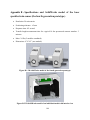
Appendix B - Specifications and SolidWork model of the laser speckle strain sensor (the fourth
generation prototype) ....................................................................................................... 104
Appendix C - Uncertainty Analysis ......................................................................................... 105
Appendix D - Strain Sensor User’s Manual ............................................................................. 108
Appendix E - Source code ....................................................................................................... 118
viii
List of Figures
Figure 1-1 Whittemore gauge ......................................................................................................3
Figure 1-2 Prestressed concrete with metal points mounted on the surface ..................................4
Figure 1-3 Electrical resistance strain gauge ................................................................................4
Figure 1-4 Fiber Bragg Gratings ..................................................................................................7
Figure 1-5 Transmission and reflection of Fiber Bragg Grating (Merzbacher, 1996)....................7
Figure 1-6 Video extensometer configuration ..............................................................................9
Figure 1-7 Speckle Generation Principle ...................................................................................10
Figure 1-8 Speckle Pattern ........................................................................................................ 10
Figure 1-9 Microstar® Strain gauge ..........................................................................................11
Figure 1-10 ME-53 laser speckle extensometer .........................................................................13
Figure 2-1 Imaging system of recording the speckle pattern ...................................................... 17
Figure 2-2 Plot of speckle intensity distribution function ...........................................................21
Figure 2-3 Tilt-Only Plane and Translation-Only Plane ............................................................. 22
Figure 3-1 5-Axis Measurement Imaging System ......................................................................30
Figure 3-2 Breadboard prototype for the 5-Axis motion measurement system ........................... 30
Figure 3-3 Single module design ............................................................................................... 32
Figure 3-4 Image splitting .........................................................................................................32
Figure 3-5 Prototype based on single module design .................................................................33
Figure 3-6 Interior view of the prototype based on the single module design .............................33
Figure 3-7 Strain Measurement ................................................................................................. 34
Figure 3-8 Dual module design ................................................................................................. 37
Figure 3-9 Schematic of the dual module design with dimensions labeled ................................. 38
Figure 3-10 The third generation prototype based on dual module design .................................. 40
Figure 3-11 Interior view of the individual module of the third generation ...............................40
Figure 3-12 The fourth generation prototype based on dual module design................................42
Figure 3-13 Interior view of the fourth generation prototype ..................................................... 43
Figure 3-14 Experiment to evaluate thermal expansion effect .................................................... 44
Figure 3-15 Saw-tooth laser beam profile ..................................................................................45
Figure 3-16 Gaussian laser beam profile .................................................................................... 45
ix
Figure 3-17 Laser pointing stability test ....................................................................................47
Figure 3-18 Multiple modules setup ..........................................................................................48
Figure 3-19 Rosette setup for two dimensional strain measurement ........................................... 49
Figure 3-20 Visible markings and supporting legs used as the alignment mechanism ................50
Figure 4-1 Image processing diagram ........................................................................................51
Figure 4-2 Histogram equalization ............................................................................................ 52
Figure 4-3 A typical speckle image and its frequency spectrum ................................................. 53
Figure 4-4 Hanning window ...................................................................................................... 54
Figure 4-5 Filtered speckle image and its frequency spectrum ................................................... 54
Figure 4-6 Pyramid scheme ....................................................................................................... 56
Figure 4-7 Sub-image scheme .................................................................................................. 57
Figure 4-8 Zero padding interpolation .......................................................................................59
Figure 5-1 Camera image distortion ..........................................................................................63
Figure 5-2 Image pairs for the camera distortion experiment ..................................................... 64
Figure 5-3 Misalignment between the initial reading and the second reading .............................65
Figure 5-4 Misalignment between the two modules of the sensor .............................................. 67
Figure 5-5 Transformation from object coordinates to camera coordinates ................................ 68
Figure 5-6 Homography Projection from objection coordinate to camera coordinate .................69
Figure 5-7 Setup of the first calibration method ......................................................................... 71
Figure 5-8 Strain calculation with orientation difference of the two camera coordinate systems 74
Figure 5-9 Messphysk company’s laser speckle extensometer ME53-33 ...................................75
Figure 6-1 A two concrete block system .................................................................................... 81
Figure 6-2 Comparison of laser speckle strain sensor and Digital dial gauge .............................81
Figure 6-3 Difference between optical strain sensor and digital dial gauge measurements .........82
Figure 6-4 A concrete beam under compression ........................................................................ 83
Figure 6-5 Surface deflection measurement obtained by Whittemore gauge and laser speckle
strain sensor.......................................................................................................................83
Figure 6-6 Experiment setup of the comparison of laser speckle strain sensor and electrical
resistance strain gauge (ESG) sensor .................................................................................84
Figure 6-7 Measurement results of surface strain.......................................................................85
x
Figure 6-8 Difference of the measurements between optical strain sensor and electrical resistance
strain sensor.......................................................................................................................85
Figure 6-9 Metal points bonded onto the concrete surface ......................................................... 86
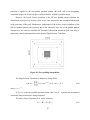
Figure 6-10 Cross-section of the pretensioned concrete member................................................ 87
Figure 6-11 Experiment setup for transfer length measurement of prestressed concrete member
using the second generation prototype ...............................................................................88
Figure 6-12 Comparison of strain measurements immediately after de-tensioning of a pretensioned specimen............................................................................................................ 88
Figure 6-13 Optical surface-strain measurements during the first 28-days after de-tensioning .. 89
Figure 6-14 Experiment setup for the transfer length measurement of prestress concrete member
using fourth generation prototype ...................................................................................... 90
Figure 6-15 Concrete surface strain measurements immediately after de-tensioning of a pretensioned specimen using laser speckle strain sensor ......................................................... 91
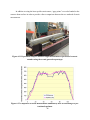
Figure 6-16 Laser speckle strain sensor mounted on a rail at CXT concrete cross-tie plant ........92
Figure 6-17 Severe abrasions to the cross-tie surface at the saw-cutting machine.......................94
Figure 6-18 Cross-tie surface bonded with microscopic reflective particles ............................... 94
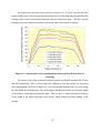
Figure 6-19 Cross-tie surface strain measurement (Tie 1 Side A) .............................................. 95
Figure 6-20 Cross-tie surface strain measurement (Tie 2 Side B) ............................................... 95
Figure 6-21 Cross-tie surface strain measurement (Tie 3 Side A) .............................................. 96
xi
List of Tables
Table 5-1 Data of the camera distortion experiment...................................................................64
Table 5-2 Error caused by the sensor misalignment ...................................................................66
Table 5-3 Calibration data from camera A and camera B........................................................... 72
Table 5-4 Experimental data of the Auto Calibration method demonstration .............................77
Table C-1 Experiment data for uncertainty analysis................................................................. 106
xii
Acknowledgements
I wish to express appreciation to my advisor, Dr. B. Terry Beck, for his friendship and
guidance.
I would also like to thank Dr. Robert J. Peterman and Dr. Chih-Hang (John) Wu, with
whom I have worked throughout my graduate study, for their valuable advice and insight into my
research. Thank Dr. Youqi Wang and Dr. Ruth Douglas Miller for reviewing my thesis.
There are many collaborators to whom I owe my appreciation. These include Rob
Murphy, Steven Hammerschmidt and Ed Volkmer, with whom I conducted extensive testing and
many experiments using the laser speckle strain sensor. Trevor Heitman and Ryan Benteman
also provided excellent technician support for the fabrication of the sensor. The sensor has been
greatly improved due to their work.
I am also grateful of Kansas Depart of Transportation (KDOT), University Transportation
Center (UTC) , Advanced Manufacturing Institute (AMI) and Precast/Prestressed Concrete
Institute (PCI) for their kind financial support.
xiii
Dedication
To my wife Grace.
xiv
Chapter 1 - Introduction
1.1 Background of strain measurement for civil infrastructure
Civil engineering infrastructure comprises some of the most massively built assets in the
world. For centuries, engineers have been trying to build more reliable and long-lasting
infrastructure, from the Great Wall in China to the modern Interstate Highway System in the
USA. Many new materials and design concepts have been proposed aimed at reducing weight,
increasing spans, achieving longer infrastructure life and lower cost. However the civil
engineering field has been conservative in adopting the new materials and technologies due to
concern for compromising safety standards (S C Liu, 1995)(Faber & Stewartb, 2003). This
resulted in a relatively slow evolution of technologies in the field of civil engineering compared
to those of other disciplines such as computer science and electronic engineering. The barrier in
adopting the new materials and technologies lies partly in the lack of convenient and reliable
methods to evaluate their performance and implement safety control.(S C Liu, 1995)
In addition, civil infrastructure is usually designed with a large margin of safety, with the
nominal load 2 or 3 times of the actual load (A.A. Mufti, 2008). However, the aging of the
structure and excessive usage always lead to a reduced factor of safety. For instance, it is
reported that more than 200,000 bridges in United States and 30,000 bridges in Canada are
operating at a deficient condition due to the inadequate maintenance and excessive loading.
(Mufti, 2003). It is risky to keep the aged civil infrastructures in service without reliable
information of them.
Either to design and build civil infrastructures of extended lifetime without
compromising the safety or increased cost, or to effectively qualify their performance in the term
of safety, it is important to find a convenient way to collect the information about the structure
performance, either at time of the construction or at the time of service. One of the factors that
are always used to evaluate the performance of concrete member is the stress or strain
information in the member. For example, the evaluation of the bridge health is usually done by
measuring the in situ strain responding to traffic flow. (Ceravolo, 2005).
1
Of particular importance to civil infrastructure is prestressed concrete, which is usually
fabricated by casting concrete mix around already tensioned steel strands. After the casting
process is complete and the concrete has hardened, a detensioning procedure is undertaken by
cutting the reinforcing strands at both ends of the concrete beam to release the tension. The
stress transferred from the strands to the concrete is developed gradually from each end of the
beam, where the stress is zero, and to the location far away from the end, where the stress is at its
full value. The distance required to develop this stress is defined as “The transfer length”, which
is used to evaluate the quality and performance of concrete members. To estimate the transfer
length, the surface strain profile of the prestressed concrete beam must be measured.
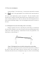
Many methods are available to measure strain either on the surface or in the body of the
concrete structures. The strain measurement under laboratory conditions is usually
straightforward, but it is much more difficult when applied in the field due to the fact that most
of the strain measurements of structure materials must be done in a harsh environment, or require
long term monitoring. In addition, it is recognized that a measurement technique that aimed to
make its way to the diagnostic testing of large concrete structures, must be easy to use. Most
civil engineers, particularly field engineers, are not experts in sophisticated sensor technology.
Therefore, it is important to provide them with a practical solution instead of just a laboratory
device with nanometer level resolution but could not be readily used in the field with minimum
training. To be incorporated into the diagnostic testing of modern concrete structures seamlessly,
the sensor must be able to provide rapid working speed and not require any special training of
the workers.
The characteristics desired for a strain sensor suitable for diagnostic testing of prestressed
concrete members in the field include:
Robustness
Portability
Adequate sensitivity and dynamic range
No contact to the surface
Insensitivity to out-of-plane motion of the surface
Insensitivity to environmental temperature fluctuation
Removable from the surface during downtime
2
1.2 Literature review of strain measurement techniques
In this section, several available strain measurement techniques are discussed.
1.2.1 The Whittemore gauge
Figure 1-1 Whittemore gauge
The Whittemore gauge as shown in Figure 1-1 is a mechanical strain gauge that has been
widely used for measuring surface strain of concrete structures for decades. Before a strain
reading can be made, small steel circular buttons with a precision pinhole at the center, called
“points”, are bonded on the concrete surface by using epoxy as shown in Figure 1-2. The
Whittemore gauge measures the distance between the pinholes of successive pairs of points.
Prior to the surface deformation, a set of reference length measurement are made, representing
the unstrained positions of the points. Then a second measurement is taken after the surface
deformation. The difference between the second measurement and the reference length is divided
by the gauge length 203.2mm (8”), giving the strains on the concrete surface. When a reasonable
strain profile is required, tens of points must be bonded onto the concrete surface, which is very
time-consuming and labor-intensive. Furthermore, the measurement results are heavily
influenced by the users’ habits and skills. Experience shows that different users can produce
readings that are greatly different. It requires a considerable amount of training and experience to
achieve consistent and repeatable results.
3
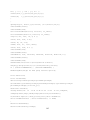
Figure 1-2 Prestressed concrete with metal points mounted on the surface
1.2.2 Electrical resistance strain gauge
Another traditional gauge used to measurement concrete surface strain is the electrical
resistance strain gauge (MUSPRATT, 1969). It employs the principle that metallic conductors
subjected to mechanical strain exhibit a change in their electrical resistance. By converting
mechanical strain into an electronic signal, the electrical resistance strain gauge can measure
strain to quite high resolution.
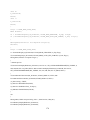
Figure 1-3 Electrical resistance strain gauge
In general, the electrical resistance strain gauge is precise, reliable and easy to use.
However, the technique has several disadvantages.
4
The technique requires gluing the gauge on the specimen surface. Since the gauge
has contact with the specimen surface, it may influence the surface strain and cause
measurement error.
It is difficult to bond the gauge to the rough surface such as concrete.
Temperature, material properties and the adhesive that bonds the metallic
conductors to the surface all affect the detected resistance, and hence can interfere
with the accuracy of the strain measurement. (A. L. Window, 1982)
The electrical resistance strain gauge is sensitive to electromagnetic interference
(EMI), which could cause measurement error when used in the industrial
environment where many types of EMI inducing equipment are present, such as
motors or electrical heaters.
In a harsh environment, the glue may debond and the gauge may break off from the
specimen surface, making the measurement impossible.
In the case of large and suddenly changing surface strain, the gauge may suffer
from “creep effect”. Experiments have shown that the reading of the electrical
resistance strain gauge tends to decrease from an initial value if the specimen
surface is subjected to a suddenly large load. The creep effect is caused by the
partial debonding of the glue that bonds the gauge to the surface, which results in
measurement error (Brinson, 1984).
5
1.2.3 Vibrating wire strain gauge
The vibrating wire strain gauge operates on the principle that the natural frequency of a
pretensioned wire is affected by the stress applied to it. The relationship between the natural
frequency f and the stress
is described by (A. L. Window, 1982)
f
where
1
2l
(1.1)
is the wire material density and l the length of the wire.
The vibrating wire gauge is very simple in design. Two anchors are installed on the
specimen surface and the two ends of the wire are attached to the anchors. Once the stress
of
the wire is known using Equation (1.1) , the strain of the surface can be found too, assuming the
wire deformation faithfully follows the surface deformation. The advantage of the wire vibration
gauge is that the gauge (wire) can be removed from the specimen, which makes it a suitable tools
for long-term monitoring of strain change in the concrete structure. The major drawback of the
wire vibration gauge is its sensitivity to ambient temperature. It is reported that a 1 degree
temperature change causes a 20
change in the strain measurement (Neild, 2005). In some
situations the specimen temperature changes rapidly, either due to ambient temperature change,
or due to active heating to the concrete mix to expedite the cure process. Unless the thermal
expansion factor of the specimen is the same of that of the wire, measurement error is
introduced. It is possible to compensate the error caused by the temperature change, but doing so
greatly complicates the system.
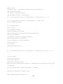
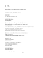
1.2.4 Fiber optics strain sensor
Fiber optics based measurement techniques are very versatile. As many as 60 different
quantities, including temperature, pressure and strain can be measured by fiber optics. (Fuhr,
2000). For strain measurement, Fiber Bragg Grating is one of the most popular methods in recent
years. The optical fiber used in this method is fabricated in a way that there is a periodic
6
variation of the refractive index in the fiber core, called a “Bragg grating”. Suppose the grating
interval is G , as shown in Figure 1-4, The Bragg wavelength is calculated by
2 n G
(1.2)
where n is the average refractive index.
When incident light passes through the Bragg grating, only the light of the wavelength
equal to the Bragg wavelength will be reflected and the light of the wavelength other than the
Bragg wavelength transfers through. Since the Bragg wavelength
is dependent on the Bragg
grating interval G , which is in turn directly related to the applied strain, the applied strain can be
determined by measuring the Bragg wavelength, i.e. the wavelength of the reflected light.
Figure 1-4 Fiber Bragg Gratings (Merzbacher, 1996)
Figure 1-5 Transmission and reflection of Fiber Bragg Grating (Merzbacher, 1996)
Fiber Bragg Grating method has several advantages over the traditional eletrical
resistance strain sensor. First, it is immune to electromagnetic interference from the industrial
enviroment (Merzbacher, 1996). In addition, it does not suffer from any light intensity
fluctuation in that it measures the strain based on the change of the reflected light wavelength,
which is an absolute quantity. However, there are several drawbacks associated with the Fiber
Bragg Grating method.
7
To measure the specimen strain, the optical fiber can be either be mounted onto the
surface or embedded in the body of the specimen. When the fiber is embedded in the
concrete mix, the alkaline chemical environment starts to erode the thin coating that
protects the fiber core. For long term strain measurement, the aging of the fiber might be
a problem or even cause the loss of the measurement. The protection of the leads of the
fiber that exit from the concrete surface is also a concern in field applications of the
method.
It is questionable how faithfully the strain of the fiber follows the change of the strain of
the specimen. The loss of grip (debond) between the fiber and the concrete mix might
happen, causing a difference of the strain between them.
It is reported that when the FBG fiber is not aligned to the principal stress direction of the
host material, the strain detected by the FBG sensor will be much different than that of
the host material. (Hong-Nan Li, 2007)
1.2.5 Video extensometer
A video extensometer measures the surface strain by tracking the coordinates of
contrasting marks placed on the specimen. The gauge marks can be in the form of grid of dots or
lines as shown in Figure 1-6, with the dot diameter or line thickness ranging from half millimeter
to a couple of millimeters. The video image captured by the digital camera is analyzed by the
image processing algorithms to locate the centers of the dots or the edges of the lines. During the
test, the centers of the dots or the edges of the lines are followed automatically by the software.
Their coordinate changes are used to extract the specimen strain information (Malo, 2008).
8
Figure 1-6 Video extensometer configuration (Malo, 2008)
Since the surface strain is measured by tracking a center of the mark, fine marks must be
applied to the surface, such as a 7x7 grid of 0.5 mm diameter dots as described in wood surface
strain measurement (Malo, 2008). For a material with irregular or soft surface, the application of
marks may not be practical.
Some other Video extensometers, such as the MTS LX Laser Extensometer (MTS LX
laser extensometer, 2009), use tapes instead of marks to tag the surface displacement. The tape
that attaches to the specimen surface has strip spacing on it. The extensometer determines the
surface strain by measuring the extension of the strip spacing. The technique is not a real noncontact measurement method since the tape contacts the specimen surface. It is possible that the
strip and the specimen extend or shrink by different amounts due to a creep effect, so that the
strain measured from the tape does not faithfully represent the actual specimen strain. The
resolution is limited by tape strip spacing and usually low.
1.2.6 Laser speckle strain measurement
Speckle is generated by illuminating a rough surface with coherent light as shown in
Figure 1-7. The random reflected waves interfere with each other, resulting in a grainy image, as
shown Figure 1-8. The speckle pattern could be thought of as a “fingerprint” of the illuminated
area in the sense that the speckle pattern produced by every surface area is unique. Furthermore,
when the surface area undergoes movement or deformation, the speckle pattern in the image
plane will also move or deform accordingly.
Most optical speckle methods for in-plane displacement or deformation measurements
are based on the same principle. That is, the grainy speckle pattern image is recorded before the
9
surface is deformed and after the surface deformation. The deformation or displacement
components can then be extracted by comparing the speckle patterns before and after a surface
deformation. This is typically done statistically using a cross-correlation technique to measure
the speckle displacement.
(See Section 2.4 for detailed discussion of cross-correlation
technique)
C oh eren t L igh t
So urce
In Ph aseBrigh t S p eck le
O u t o f P h aseD ark S p eck le
S urface
F ilm P lane
or D etector
Figure 1-7 Speckle Generation Principle
Figure 1-8 Speckle Pattern
There exist two basic categories of speckle technique for surface strain measurement:
electronic speckle pattern interferometry (ESPI) and digital speckle photography (DSP). They
relate to different methods of producing and processing the speckle image. The ESPI technique
measures the object surface displacement or deformation by detecting the corresponding phase
change of the light wavefronts reflected from the surface, just as a conventional Michelson
interferometer does. The image taken in an ESPI system, called a “speckle interferogram”, is
produced by interfering the speckle radiation reflected from an object surface with a reference
10
light field, either a uniform coherent light beam or another speckle field (Dainty, 1975). In
practice, the speckle interferograms are taken both before and after the object displacement or
deformation. A characteristic fringe pattern can be obtained by subtracting the two speckle
interferograms. The fringe spacing corresponds to a 2
phase change of the wavefronts resulted
from the object surface deformation, as is the case with a Michelson interferometer with a mirror
displacement. Thus the surface deformation and displacement can be readily determined by
counting the number of fringe changes. As an interferometry method, the ESPI technique has
high resolution on the order of a fraction of a light wavelength, and the resolution is not limited
by the resolving power of the imaging system (Samala, 2005) (Helena (Huiqing) Jin, 2006). As
fringe counting is involved, this method has a 2
ambiguity limitation; that is, the periodical
fringe pattern resembles itself whenever it shifts by an integer multiple of 2
phase. There is no
easy way to determine the phase change uniquely. Another limitation is in the upper bound of the
deformation that can be measured, due to the limited number of visible fringes on the detector
(typically a CCD array) (C. Joenathan, 1998).
Figure 1-9 Microstar® Strain gauge
Fig 1-9 shows a commercial full field strain sensor named Microstar® based on ESPI
technique. It has the ability to automatically analyze the geometry and the deformation of the
surface area of interest within 100nm resolution. Due to its miniature size, the sensor can be
easily attached to the components during testing and has received a wide acceptance in
11
automobile and aerospace industries.(L.X. Yang, 1999)(R.Wegner, 1999). The Microstar® strain
sensor requires stringent alignment with the specimen surface and must be fixed onto the
specimen surface throughout the measurement process to prevent rigid relative movement. This
drawback makes it impractical to be used for strain measurement for civil engineering structure,
where either long term monitoring of the surface strain is required, or enormous shock happens
to the subject such that the sensor must be removed to avoid damage. For instance, a prestressed
concrete beam is subjected to a nominal 30,000lb sudden force during the detensioning of the
steel strands and this may damage the sensor if left on the concrete surface.
The DSP technique, on the other hand, is based on intensity correlation. By comparing
two speckle images, taken before and after surface deformation, the in-plane displacement vector
resulting from the loading can be determined. Once the complete displacement field is obtained,
it can be differentiated to obtain an in-plane strain map. DSP generally has lower resolution than
ESPI, but larger dynamic range. The resolution is limited by the speckle size, which typically
ranges at the micrometer level, and the resolving power of the imaging system. There exists
some strain measurement devices in the market utilizing DSP technique. One of them is ME-53
extensometer (ME-53 Laser speckle extensometer manual)(Eduard Schenuit, 2008) from
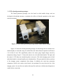
Messphysik company. It has two variations. One version consists of two cameras and a servo
drive that controls the motion of the cameras for a large gauge length setup, as shown in Figure
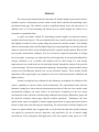
1-10; the other version consists of a single camera for small area surface strain measurement.
The ME-53 laser speckle extensometer makes non-contact strain measurement based on the DSP
technique and does not require any surface marking.
However it is mainly designed for
laboratory use. The sensors must be mounted on a vertical track and the specimen must be
installed on a laboratory bench. This is to prevent the relative rigid motion between the sensor
and the specimen. Although the DSP technique is designed to measure in-plane movement, it is
also commonly sensitive to surface tilt (yaw and pitch), which brings error into the strain
measurement.
The bulky size of the system also makes the system impractical for use in the
field. Furthermore, a calibration procedure involving displacement of the camera by a certain
known distance using the servo system that comes with the system must be conducted by the end
user prior to the measurement. In addition, whenever the distance between the sensor and the
specimen surface changes, the system must be re-calibrated.
12
Figure 1-10 ME-53 laser speckle extensometer
1.3 Overview of dissertation
The importance of having a reliable and robust strain measurement technique for either
factory monitoring or “field testing” of concrete structural members has been described above.
The current available methods are either more opted for laboratory testing or are too slow to
allow online monitoring.
The work presented in this dissertation illustrates the development of a general strain
measurement technique based on the laser speckle principle that is able to rapidly and accurately
determine concrete surface strains. An understanding of the relationship between the multidegree motion of the subject surface and the induced motion of the speckle pattern is required in
order to make the laser speckle measurement technique applicable to the typically harsh
industrial environment. A portable prototype incorporating unique modular design concept and
self-calibration feature has been fabricated. The portable design enables flexible adjustment of
the gauge length and easy expansion to a rosette strain measurement configuration.
Extensive testing has been conducted in the laboratory environment to validate the
sensor. Furthermore, the laser speckle strain sensor was applied to transfer length measurement
of common prestressed concrete beams, and prestressed concrete cross-ties in the field. The
sensor yielded unprecedented measurements of transfer length in just a few minutes, compared to
the hours that are needed if using the current accepted method of measurement.
13
Through this testing with different applications, it has been shown that the newly
developed portable laser speckle strain sensor can not only serve as an accurate instrument in the
civil engineering laboratory where the deflection characteristics of a concrete member are
needed, but also can be readily used in the harsh environment of the prestress concrete industry,
with minimum surface preparation and staff training. It also has the potential to rapidly process a
large quantity of data points in an industrial setting.
It should be noted that, as far as the author is aware, the new developed sensor is the first
device to successfully employ speckle method to determine transfer length of prestressed
concrete. Furthermore, this development represents the first time that such a method has been
demonstrated successfully in a harsh industrial environment with sufficient resolution and
accuracy, to make automated transfer length measurement possible in the concrete railroad crosstie manufactory industry.
The chapters in this dissertation are arranged as follows:
Chapter 2: Theoretical background of the laser speckle strain measurement
Theoretical modeling of the speckle will be presented, using Fourier optics. The
principle behind the 5-axis motion measurement, which serves as the foundation
of the design of the laser speckle strain sensor, will be discussed. The digital
image correlation technique, which is the crucial part of the data analysis, will
also be presented.
Chapter 3: Hardware design of the optical strain sensor
Various different hardware designs of the laser speckle strain sensor will be
described in detail. Their advantages and drawbacks will be compared. Technical
detail of the individual components including laser head, CCD camera, lens and
the alignment mechanism used by the sensor will be presented.
Chapter 4: Software development of the optical strain sensor
The preprocessing of the captured speckle images will be presented. A detailed
explanation of how the digital correlation procedure is conducted to extract the
relative shifting of the speckle patterns in sub pixel resolution will be presented,
along with the various techniques that are implemented to speed up the correlation
computation.
14
Chapter 5: Calibration
The general procedure for the calibration of the laser speckle strain sensor will be
presented. Then the effect of the sensor misalignment will be investigated. An
improved calibration method that is able to correct the error caused by the
orientation difference of the two camera coordinates will be presented.
Chapter 6: Conclusion
The work that has been done for the development of the laser speckle strain
sensor will be summarized. The recommendation of future work based on the
efforts presented here will be discussed.
The appendices at the end of the dissertation contain the references cited in the text. The
hardware components list and the specifications for the sensor, along with the uncertainty
analysis, are also included. An operation manual for the laser speckle strain sensor and the
software source code are attached to the end of the dissertation.
15
Chapter 2 - Theoretical
background
of
laser
speckle
strain
measurement technique
Speckle is generated by illuminating a rough surface by coherent light. The reflected light
interferes constructively and destructively, creating a grainy pattern at the observation plane. In
this chapter, Fourier optics, statistical tools and imaging theory are used to explore the various
characteristics of the speckle. The characteristics of the speckle are described mathematically
and the optimal spatial sampling resolution is obtained. Furthermore, the theory of 5-axis motion
measurement technique will be described. The 5-axis motion measurement was developed at the
early stage of the optical strain sensor development. It is important to the strain sensor
development in that the object surface during deformation is usually subjected to 6 degrees of
freedom movement. However, only the in-plane displacement information is used to calculate
the strain. The motion of other axis, especially the out-of-plane rotations act as error source to
the strain measurement. The 5-axis motion measurement system is able to separate the 5-axis
movement so that the movement of each axis can be measured independently, thus the effect of
the out-of-plane rotations can be eliminated for the strain measurement. To the end, the digital
image correlation technique is discussed. It is an image process technique that estimates the
relative shift of the speckle image pairs taken before and after the surface deformation, such that
the displacement or strain information can be extracted.
2.1 Mathematical description of the speckle phenomenon
Speckle is generated by illuminating a rough surface with coherent light, as shown in
Figure 1-7. The random reflected waves interfere with each other, resulting in a grainy image, as
shown Figure 1-8.
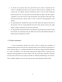
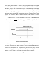
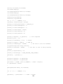
Figure 2-1 shows an imaging system of recording the subjective speckle filed by a CCD
camera. The object plane XY is illuminated by a laser light beam. The reflected laser lights from
the rough object surface is collected by the lens and then imaged onto the camera plane xy from
the object. The distance between the lens and the object plane is do and the distance between the
16
camera plane and the lens is di . For surface deformation measurement, the speckle images are
recorded twice by the camera, before and after the surface deformation.
Figure 2-1 Imaging system of recording the speckle pattern
The amplitude response of a point source at coordinate (0,0) on the object plane XY ,
which is also the impluse response function of the optical imaging system,
is defined as
(Goodman, 1996)
h( x, y)
P( d i x ', di y ') exp[ j 2 ( xx ' yy ')]dx ' dy '
(2.1)
where P( di x ', di y ') is the pupil function
P( di x ', di y ')
1
x '2 y '2
0
D
2 di
(2.2)
otherwise
where D is the diameter of the lens pupil and ( x ', y ') is the coordinate on the lens plane.
Denoting
x '2 y '2 , we have
x'
Further define r
x2
cos
y'
sin
(2.3)
r cos
y
r sin
(2.4)
y2
x
17
Substituting Equation (2.3) and Equation (2.4) into Equation (2.1), and implementing the
polar integral,
D
2 di 2
h( x, y )
exp[ j 2
0
r cos(
)] d d
(2.5)
0
Since the Bessel function of the first kind is defined as
2
1
2
J 0 (u )
exp[ ju cos( )]d
(2.6)
0
we have,
D
2 di
h( x , y )
2
J 0 (2
r) d
(2.7)
0
Further using the integral identity of the Bessel function of the first kind,
u
(2.8)
u ' J 0 (u ')du ' uJ1 (u )
0
Equation (2.7) can be simplified to be
h( x, y )
J1 (2 Dr / di )
Dr / di
(2.9)
Since the optical imaging system is shift-invariant, meaning that the shifting of the input
in some direction shifts the output by the same distance and direction, for a point source location
at the coordinate ( X , Y ) on the object plane, the amplitude response at coordinate ( x, y ) on the
camera plane is
h ( x, y ; X , Y )
h( x X , y Y )
(2.10)
Since the optical imaging system is a linear system, the complex amplitude at coordinate
( x, y ) on the camera plane is the superposition of amplitude response of all the point light
sources ( X , Y ) where
X
Y
.
Assuming
uo ( X , Y )
f ( X , Y ) exp[ j 2
18
( X , Y )]
(2.11)
The convolution of the object intensity with the point spread function is
ui ( x, y)
h( x X , y Y )uo ( X , Y )dXdY
(2.12)
Denoting the Fourier transform of uo ( x, y) , ui ( x, y) and h( x, y )
Uo (
x
Ui (
H(
x
,
y
,
x
)
y
,
)
F uo ( X , Y )
(2.13)
)
F ui ( x, y )
(2.14)
y
F h( x, y )
P ( di
x
, di
)
(2.15)
D 2
)
2 di
(2.16)
y
where
P( d i
x
, di
y
2
x
1
)
0
2
y
(
otherwise
The convolution form in Equation (2.12) can be expressed in frequency domain as,
Ui (
x
,
y
)
H(
x
,
y
)U o (
x
,
y
(2.17)
)
The intensity at point coordinate ( x, y ) on the camera plane is,
s ( x, y )
2
ui ( x , y )
ui ( x, y )ui * ( x, y )
(2.18)
where ui* ( x, y ) is the conjugate of ui ( x, y)
.
Therefore, the Fourier transform of s ( x, y ) can be represented as the convolution of
Ui ( x, y) and U i* ( x, y )
S(
x
,
y
)
F s( x, y )
F ui ( x, y )ui* ( x, y )
Ui (
x
,
y
(2.19)
*
i
) *U (
x
,
y
)
Substituting Equation (2.17) into Equation (2.19),
S(
x
,
y
)
H(
x
,
y
)U o (
x
,
y
) * H *(
19
x
,
y
)U o* (
x
,
y
)
(2.20)
Observing that uo ( X , Y ) is the reflected laser light beam intensity from the rough object
surface, due to the random feature of the surface profile, both the amplitude term and phase term
are modulated randomly. Therefore uo ( X , Y ) can be regarded as a random function.
Therefore Equation (2.20) is simplified as
S(
x
,
y
)
H(
x
,
y
) * H *(
Since h( x, y ) is symmetric, we have H * (
S(
x
,
y
)
H(
x
x
,
y
,
y
x
y
)
H *(
)
)* H*(
,
x
,
y
x
(2.21)
,
y
)
)
(2.22)
Thus
s ( x, y )
h( x, y )
2
(2.23)
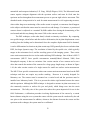
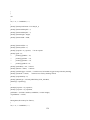
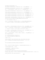
Substituting Equation (2.9) into Equation (2.23), we get the intensity distribution of the
subjective speckle pattern,
s ( x, y )
where r
x2
s(r )
J1 (2 Dr / d i )
Dr / d i
2
(2.24)
y 2 , and x, y are the coordinates at the image plane, J1 is the standard Bessel
function of the first kind, D is the lens pupil diameter, di is the image distance,
is the light
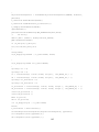
wavelength. The intensity distribution function of the subjective speckle pattern is plotted in
Figure 2-2. According to the Rayleigh criterion (Hecht, 1998), the average speckle size is
determined as the value of r where the value of the function s ( r ) drops to its first local
minimum. By setting J1 (
2 Dr
) 0 , the solution is found to be
di
2 Dr
di
3.83
(2.25)
di
D
(2.26)
which in turn gives
r 1.22
This is the average size of the speckle on the camera plane.
20
Figure 2-2 Plot of speckle intensity distribution function
2.2 Review of the 5-Axis motion measurement system
Axial strain measurement is accomplished by taking the differential of the relative
displacements between two points on the object surface. A typical speckle measurement is
fulfilled by first illuminating the associated specimen surface with coherent light (laser). The
random reflections from the surface features (roughness) generate a grainy speckle pattern image
at the camera plane. This speckle pattern could be thought of as a “fingerprint” of the illuminated
area, in the sense that the speckle pattern produced by a given surface region is unique.
Furthermore, when the surface undergoes movement or deformation, the speckle pattern in the
image plane will also move or deform accordingly. This tracking feature is the basis of the
displacement measurement of the laser speckle technology.
However, the speckle displacement at the camera plane usually is not only sensitive to
the object surface displacement, but also to other axis movements of the object surface;
especially the out-of-plane rotations (tilt and yaw), which result in error in the strain
measurement. To extract the displacements accurately without being affected by other axis
movements, a 5-axis motion measurement technique was developed that is able to separate the 5-
21
axis movement so that the movement of each axis can be measured independently, thus the effect
of the out-of-plane rotations are mostly eliminated.
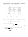
The 5-axis measurement principle is based on the fact that for subjective speckle there
exist two characteristic planes behind the lens, a ‘tilt-only plane’ and a ‘translation-only plane’,
such that the speckle image at the tilt-only plane is only sensitive to the tilt of the specimen, and
the speckle image at the “translation-only” plane is only sensitive to the translation of the
specimen. (D.A.Gregory, 1976). These planes are shown in Figure 2-3.
The 5-axis motion measurement technique was developed during the early stage of the
laser speckle strain sensor development (Zhao, 2006). The principle of the 5-axis motion
measurement was later applied to the design of the optical strain sensor in which the camera is
positioned at the ‘translation-only plane’ of the optical system to eliminate the effect of the
surface motion other than the in-plane displacement. A detailed discussion of the 5-axis motion
measurement technique can be found in author’s M.S. thesis (Zhao, 2006).
Figure 2-3 Tilt-Only Plane and Translation-Only Plane
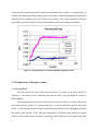
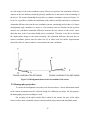
2.3 Insensitivity of system sensitivity to out-of-plane movement
During the operation of the optical strain sensor in the field, in some situations the sensor
does not work in a stationary manner. For example, for the prestressed concrete beam strain
measurement, the sensor is required to be removed from the concrete beam surface before the
22
detensioning, and then be put back on the surface after the detensioning, due to the fact that the
detensioning process involves a release of a 30000lbs (13607 kg) traction force, which could
damage the sensor if left on the concrete surface. Thus the repositioning of the laser speckle
sensor will cause the distance between the lens of the optical system to the concrete surface to
vary inevitably. This arises a problem that the change of the object distance will affect the
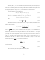
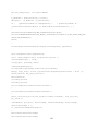
system sensitivity.
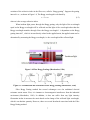
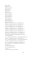
Figure 2-4 shows the measured systematic sensitivity to object translation at different
object-sensor distances. It shows that the system sensitivity varies significantly when the sensor
is at different depth positions relative to the object plane. This is obviously an undesired
characteristic for a sensor.
170
Sensitivity (pixels/mm)
168
166
164
162
160
158
156
154
97
98
99
100
101
102
103
Object distance (mm)
Figure 2-4 System sensitivity changes due to the object distance change (Zhao, 2006)
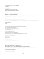
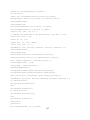
However, it is proved that under the condition of collimated and normal illumination, the
system sensitivity becomes insensitive to the out-of-plane object movement (Zhao, 2006).
Experiments, as shown in Figure 2-5, have confirmed this behaviour. In the range of 6mm
variation of object distance, the systematic sensitivity has no significant variation.
23
170
168
Sensitivity (pixels/mm)
166
164
162
160
158
156
154
97
98
99
100
101
102
103
104
105
object distance (mm)
Figure 2-5 Invariance of system Sensitivity (Zhao, 2006)
2.4 Digital correlation technique
As discussed previously, the shift of speckle image captured by the camera is
proportional to the translation of the object surface under a specific imaging setup. The issue of
detecting the surface motion is thus actually one of evaluating the relative shift of the speckle
image pairs taken before and after the surface deformation. This is done by using the digital
correlation technique.
Suppose we have two speckle images I1 , I 2 of the object surface taken before and after the
surface deformation. The traditional cross-correlation function is defined by
N
N
Corr ( x, y )
I1 (i, j ) I 2 ( x i, y
j)
(2.27)
i 1 j 1
By varying the values of x and y , the maximum value of the correlation function
Corr ( x, y ) can be found, and its coordinates give the relative components of the image
displacement. The disadvantage of the function above is that it is subjective to changes in image
intensity amplitude, generally caused by change in lighting conditions across the image
recording sequence, which are very likely to happen during a typical concrete beam strain test
24
measurement period that might last for months. To overcome the shortcomings associated to the
traditional correlation method, adapted digital correlation algorithms are more often used.
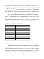
2.4.1 Normalized correlation
This method calculates the mean of the speckle image I1 and I2, then determines their
normalized version I1’ and I2’. The correlation coefficient is then obtained similar to Equation
(2.27). The result is normalized again to obtain the normalized cross-correlation coefficient.
N
N
I1 '(i, j ) I 2 '( x i, y
j)
i 1 j 1
R ( x, y )
N
N
N
I1 '(i, j )
i 1 j 1
(2.28)
N
2
I 2 '( x i, y
j)
2
i 1 j 1
where
N
N
I1 (i ', j ')
I1 '(i, j )
I1 (i, j )
i' 1 j ' 1
(2.29)
N *N
N
N
I 2 ( x i ', y
I 2 '( x i, y
j)
I 2 ( x i, y
j)
i' 1 j ' 1
N *N
j ')
(2.30)
A perfect match will give a peak equal to 1 and a complete no match will give a peak of
0. The normalization operation used by this method helps reduce effects of the image intensity
variation to the matching of the image pairs.
2.4.2 Phase correlation
Although the normalized correlation algorithm works quite well on the regular images, it
was observed that it works poorly on the speckle image. This is due to the unique characteristics
of the speckle pattern, which is a grainy pattern without any repeated feature. If the speckle
pattern is transformed to the frequency domain, it can be observed that considerable information
of the image is stored in the high spatial frequency domain, contrary to the regular image for
which most information is stored in the low spatial frequency domain. The intensity of every
speckle element in the pattern does not carry much information due to the fact that its intensity
tends to fluctuate continuously and randomly when the object surface moves. The fluctuation of
25
the intensity of individual speckle is in fact noise and should not be taken into account when
matching the speckle image pairs. Instead, it is the relative location of the speckles between the
speckle image pairs that determines if the image pairs are correlated, and the amount of relative
shifting. This explains why the normalized correlation algorithm, functioning well on the regular
images by matching the image pairs pixel by pixel according to their intensity level, does not
work well on the speckle image pairs.
Alternatively, a phase correlation algorithm based on the Fourier Transform is able to
discard the intensity information and reply primarily on the phase information for matching the
image pairs. The overall procedure using a phase correlation technique for speckle image shift
detection is described below.
Suppose a pair of speckle patterns is given, corresponding to deformed and un-deformed
states. The two speckle images can be represented as f ( x , y ) for the un-deformed one and
f ( x u, y v ) for the deformed one, where (u, v ) denotes the components of the local
displacement vector which are regarded as constants here (Zhao, 2006)
In the first step, two complex spectrums of the image pair are obtained as follow,
F1 ( 1 ,
F2 ( 1 ,
2
2
)
j2 (x
f ( x, y )e
)
f ( x u, y v)e
1
y
2)
j2 (x
(2.31)
dxdy
2)
y
1
(2.32)
dxdy
A basic property of Fourier Transform yields (Bracewell, 1978),
F2 ( 1 ,
2
)
e
j 2 (u
1
v
2)
F1 ( 1 ,
2
(2.33)
)
The normalized cross-power spectrum of the two images is then calculated as
F1 ( 1 ,
F1 ( 1 ,
) F2* ( 1 ,
2 ) F2 ( 1 ,
2
)
2)
2
e j2
(u
1
v
2)
By applying a second-step FFT to the resulting spectrum, F (e j 2
(2.34)
(u
1
v
2)
)
(u, v) , a
pulse signal appears in the second FFT spectrum image at (u,v), which represents the
26
displacement vector between the image pairs. In this approach, the FFT spectrums
F1 ( 1 ,
2
), F2 ( 1 ,
2
) consist of both magnitude information and the phase information. After the
normalization, the magnitude information is removed and only the phase information is retained.
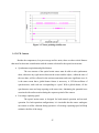
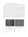
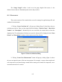
For verification purposes, a pair of speckle images with relative shifting were crosscorrelated using both the normalized correlation algorithm and the phase correlation algorithm.
The resulting correlation images were very different. In the correlation image produced by the
normalized correlation algorithm, as shown in Figure 2-6, the peak is suppressed by the high
intensity of background noise. While for the phase correlation, as shown in Figure 2-7, the peak
is very clear.
Figure 2-6 Normalized correlation results for a typical speckle image pairs
Figure 2-7 Phase correlation results for a typical speckle image pairs
27
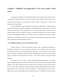
Chapter 3 - Hardware design for the optical strain sensor
This chapter discusses the hardware design of the strain sensor. Multiple factors must be
brought into the consideration during this design stage. The main objectives of the design are
listed in the following.
To develop a portable surface strain sensor capable of measuring surface strain. The
sensor dimension should be as small as possible and the weight should be light for the
portability of the sensor.
Measurement
uncertainty
to
be
on
the
order
of
25-50
microstrain
in
order to have capability similar to the Whittemore gauge whose uncertainty is about 50
microstrain.
Nominal range of measurement should be large enough to facility easy positioning and
alignment of the sensor in handheld work mode.
The sensor is aimed for a commercial product to replace the industrial standard
Whittemore gauge. Thus it should be easy to manufacture and assemble.
The sensor is to be for use in harsh environment where various condition including
extreme temperature, humid, vibration and dust pose challenge to the sensor’s function.
For example, one of the field application that the sensor has been applied to is the transfer
length measurement of railroad cross-tie in a manufacturing plant. The temperature in the
plant varies as much as 60 ºF through the year, with max temperature more than 100 ºF in
the summer. The sensor must be able to withstand harsh environments and maintain high
functional performance in operation.
Minimal training required
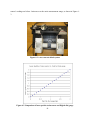
The digital speckle photography (DSP) technique that has been reviewed in Chapter 1
was chosen to be used for the development of the optical strain sensor. DSP technique has large
dynamic range, e.g. the maximum deformation or displacement that the technique can measure,
which makes it more robust than other optical strain measurement techniques based on laser
speckle. DSP technique generally has relatively lower resolution, which is limited by the speckle
28
size that typically ranges at the micrometer level. But the resolution is high enough for the
concrete beam strain measurement application.
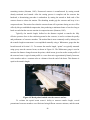
During the development of the current laser speckle strain sensor, four (4) generations of
successively improved designs have been manufactured and tested. A prototype was fabricated
for each design either on an optical breadboard for concept validation or in a portable form for
use in field testing. For each design, improvements were made based on the knowledge learned
through the testing and analysis of the prototype based on the previous generation design. The
four (4) generations of designs and their prototypes are described below in chronological order of
their development.
3.1 5-axis motion measurement system
An optical system capable of measuring the desired 5-axis (five degree of freedom)
object movement was constructed during the early stage of the current laser speckle strain sensor
development, and resulted in the author’s Master thesis.(Zhao, 2006). The 5-axis motion
measurement technique, employed in this optical breadboard layout was important to the strain
sensor development in that the object surface during deformation is usually subjected to full 6
degrees of freedom movement. The traditional optical speckle methods, though designed to
measure in-plane movement, are also sensitive to surface tilt and other rotational modes that are
very likely to happen during the concrete surface strain measurement. These rotation effects will
introduce severe error to the surface displacement or strain measurement if properly taken into
account..
The characteristics of the previously developed 5-axis motion measurement system are
described below (Zhao, 2006). The system employed the concepts of “translation-only” plane
and “tilt-only” plane to separate the surface in-plane displacement and out-of-plane tilt; thereby,
eliminating or greatly reducing rotation-induced error. The 5th axis movement (in-plane rotation)
was detected by using a polar-correlation technique. The 6th axis movement (out-of-plane
translation) of the specimen surface is shown both theoretically and experimentally to have no
contribution to the in-plane surface strain, and is therefore not measured by the sensor.
29
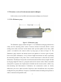
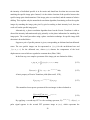
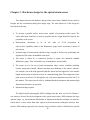
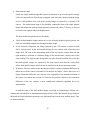
A schematic of the 5-axis motion measurement system is shown in Figure 3-1. A
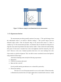
prototype of this optical system was also built on breadboard, as shown Figure 3-2. Experiments
were conducted to confirm that the system is able to separately and accurately resolve 5 axis
motion: X, Y, tilt, yaw, and roll of the specimen, with the expected insensitivity to out-of-plane
displacement (Zhao, 2006).
Figure 3-1 5-Axis Measurement Imaging System
Figure 3-2 Breadboard prototype for the 5-Axis motion measurement system
30
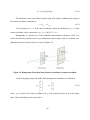
3.2 Single module design
Based on the 5-axis breadboard motion measurement system, a portable laser speckle
strain sensor was designed and fabricated utilizing one laser head and one camera
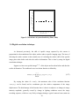
Since only the in-plane displacement components (X, Y displacements) are of interest in
the measurement of surface strain, an optical strain sensor was built to measure the in-plane
displacement components of two nearby surface points on the object surface by detecting the
speckle shifts at the corresponding “translation-only” planes only. The configuration of the
imaging system makes the sensor insensitive to any surface motion other than the in-plane
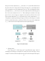
displacement. A schematic diagram of the sensor is shown in Figure 3-3. The sensor is an
integration of two identical displacement measurement systems that measure the displacements
at point A and point B, respectively.
A laser is collimated by lens L1, L2 and then directed to the specimen surface at point A
and point B respectively using polarization beam-splitter B1. The reflected waves from the
diffusive surface are directed through the beam-splitter B1 and the lens L3. Right in front of lens
L3 is a non-polarizing beam-splitter B2 that sends the reflected laser beams to Mirror M4. The
light beams then go back through the beam-splitter B2 and are finally captured by the CCD
camera. Mirror M4 is used to make the sensor more compact by folding (doubling) the optical
path length. Since there are two laser beams, reflected from point A and point B on object
surface and sent to a CCD camera, the CCD camera actually captures two speckle patterns at the
same time. The analysis of the speckle images would be more complicated if the two speckle
patterns overlapped each other. There are two approaches to prevent this from happening. One
approach involves manually blocking one laser beam at a time and taking the speckle image
twice. When the laser beam that illuminates point A is blocked, the speckle image captured by
the camera is generated by point B only. Likewise when the laser beam that illuminates point B
is blocked, the speckle image captured by the camera is generated by point A only. The other
approach is to block half of each of the laser beams with Stop 1 and Stop 2, as shown in Figure
3-3, such that only half of the areas around point A and point B are illuminated. This results in
two simultaneous side-by-side speckle patterns (Figure 3-4) on the CCD camera, generated by
point A and point B, respectively.
31
Figure 3-3 Single module design
Figure 3-4 Image splitting
The prototype of single module design and its interior view (dust cover removed) are
shown in Figure 3-5 and Figure 3-6 respectively. The optical system was built using the Cage
System® components from Thorlabs company for rapid fabrication. The camera is a Marlin
32
F145B CCD camera with a resolution of 1392 by 1040 pixels. All the optics components, the
camera and the laser head are mounted on a single piece of 8”x2” steel base. The sensor were
enclosured in a metal box with the dimension of 11”x7”x4”. The mass of the sensor is 7 lbs.
Figure 3-5 Prototype based on single module design
Figure 3-6 Interior view of the prototype based on the single module design
During the measurement, the optical strain sensor is first positioned onto the concrete
surface before the detensioning. The CCD camera then captures a speckle image of the two side33
by-side speckle patterns as shown in Figure 3-4, which are generated by point A and point B,
respectively. These two patterns are denoted as A1 and B1. The sensor is then removed from
the concrete surfaces. After the detensioning, the optical sensor is positioned (mounted) back
onto the surface. The camera captures another speckle image with two speckle patterns, which
are denoted as A2 and B2. By applying a cross-correlation technique to the pair of speckle
patterns A1 and A2 (before and after the detensioning processes), the displacement
extracted. The displacement
A can be
B can be extracted from pattern B1 and pattern B2 in a similar
fashion.
As shown in Figure 3-7, the axial surface strain, , between point A and point B can thus
be determined from
B
A
L
, where L is the gauge length 203.2 mm (8 inches) for the
current setup.
Figure 3-7 Strain Measurement
The single module strain sensor was extensively tested in a laboratory environment as
well as on actual prestressed concrete beams in the field. The measurement results were
compared with those obtained using traditional gauges (Whittemore gauge and the electrical
resistance strain gauge) and showed good consistency. The experiments and applications are
discussed in detail in Chapter 6. A provisional patent was also granted for the design.
34
The laser speckle strain sensor based on the single module design, although proved to be
a working unit, suffered from the following drawbacks:
Assembly
The single module design made use of one set of optical system component to capture
the images of two areas on the object surface. To achieve this, three mirrors (M1, M2,
M3) in Figure 3-3 are used in the system. The laser light had to be spilt and directed to
the two surface areas to be measured using these three mirrors. At the same time the
three mirrors were also used to direct the reflected light from the two separate areas on
the object surface onto the single camera, whose size was only 6.4mm by 4.8mm. The
two-folded adjustment of the three mirrors proved to be a very difficult task.
Gauge length
With the single module design, the gauge length was fixed after the sensor was
assembled. To change the gauge length, the whole system would have to be redesigned
and rebuilt.
Measurement range
The single module design integrated two identical displacement measurement systems
into one system by sharing the lens and camera. To prevent the images of the two surface
areas from overlapping each other on the single camera, a mechanism was taken to
separate the two speckle images. One of the approaches involved manually blocking one
of the two laser beam at a time. This required additional manual operation by the user and
significantly reduced the measurement pace. The other approach was to block half of
each of the laser beams, which resulted in two side-by-side speckle patterns on the CCD
camera. Each speckle pattern used only half area of the CCD chip, as shown in Figure 34. However, this approach causes the measurement range of the sensor be halved.
Weight
The prototype sensor weighed 7lbs. It makes the user fatigue quickly when the sensor
was operated in manual mode and was handheld by the user.
35
3.3 Dual module design
In observing the drawbacks associated with the single module design, the next generation
of the sensor took the form of modular design, which consisted of two identical modules that
were attached to each other rigidly side by side. The new sensor detects the displacement at two
points (usually 8 inches apart, but adjustable) on the specimen surface, which is converted into
the surface strain by dividing the net displacement by the gauge length. The displacement
measurement is based on the Digital Speckle Photography (DSP) technique. The principle of the
measurement technique is as follows: A typical measurement is fulfilled by recording the speckle
images before and after the object displacement or deformation. The two images are then crosscorrelated and the peak position of the correlation image indicates the displacement of each ends.
A schematic of the dual module design is shown in Figure 3-8. The two individual
modules are identical, except that one is a “right handed module” and the other is a mirrorarranged (or left-handed) copy of the right-handed module. Each of the modules consists of a
5mW diode laser head that emits laser light of 635 nanometers wavelength, which is then
expanded by lens L1 (12.7mm focal length) and lens L2 (35mm focal length) into a collimated
laser light of 10mm diameter. The expanded laser light is then directed to the specimen surface
by a beam-splitter B1. The reflected waves are imaged at a magnification of unity by the lens L2
onto a CCD image sensor of 1392x1024 pixels whose output signal is then sent to a PC for data
processing. The image sensor is a monochrome Lu130M CCD camera powered by 5v DC with 4
Watts power consumption. The whole optical system for individual module was rigidly mounted
on single metal base to keep the relative position of the optics components fixed. The two
modules were then rigidly attached together to keep the gauge length of the sensor constant.
36
Figure 3-8 Dual module design
It is notable that the lens L2 serves two purposes in the system. It collimates the laser
light and also images the reflected speckle pattern to the camera. Since the imaging system is a
conjugate configuration, a double convex lens is required. However, regular convex lenses with
spherical surface suffer spherical aberration, which distorts the speckle image and introduces
measurement error. The lens actually used in the optical strain sensor is a triplet lens that
consists of three single lenses, one convex lens and two concave lenses. The positive aberration
from the convex lens and the negative aberration from the concave lens are cancelled out. This
setup dramatically reduces the distortion of the imaging system.
A schematic of the dual module design with current nominal dimensions labeled is shown
in Figure 3-9.
37
Figure 3-9 Schematic of the dual module design with dimensions labeled
Since the basic methodology of single module design and dual module design are similar
,it would appear that strain sensors based on either design should be able to measure the strain
with comparable resolution. However, in terms of the practical functionality and performance,
the dual module design is more preferable for the following reasonings:
Assembly
Unlike the single module design that requires tedious adjustment of multiple mirrors
during the assembly process, the dual module design does not require any mirrors, so it is
almost adjustment free.
Gauge length
With the dual module design the adjustment of the gauge length is very easy. All the user
needs to do is to unscrew the two modules from the rods or bars that connect the two
modules together, adjust the distance between the two modules to achieve the desired
gauge length, and then re-tighten the screws to fix the locations of the two modules.
With the auto calibration feature that will be discussed in Chapter 5, the calibration of
the system parameters takes less than five minutes and can be done in the field without
the need for special additional calibration equipment.
38
Measurement range
Unlike the single module design that requires mechanisms to prevent the speckle images
of the two inspected area from being overlapped with each other, the dual module design
is free of this problem since each of the speckle images is captured by a separate CCD
camera. The measurement range is also doubled, compared to that of the single module
design that adopts the splitting image approach, because the entire CCD array is devoted
to measure the separate end-point displacement.
The dual module design also has its drawbacks:
Since the dual module design consists of two sets of nearly identical optical systems, the
total cost is doubled compared to the single module design.
As an electronic component, the image captured by the CCD camera is subject to drift
due to various noises. In the dual module design, the two cameras each suffer their own
image drift. The sum of the independent drifts of the two speckle images from left and
right modules is reflected as a distance change in the measurement, causing error in the
strain reading. The single module design does not suffer from this problem due to the fact
that both speckle images are captured by the same camera such that the camera drift
affects both speckle images, which in turn is canceled out in the measurement results.
In practice, the two cameras in the dual design will have a minor orientation difference no
matter how well the sensor is assembled. The analysis in Chapter 5 shows that even a 0.4
degree orientation difference can cause an error comparable to the nominal resolution of
the sensor if not taken into account. To deal with the problem caused by the orientation
difference of the two cameras, a more complicated calibration algorithm has to be
implemented.
Overall the traits of the dual module design overweigh its disadvantages. Efforts were
subsequently expended on its implementation and perfection of the dual module design. Both the
third and the fourth generation prototypes are fabricated based on the dual module deign. They
are discussed below.
39
3.3.1 The third generation prototype
Figure 3-10 shows the third generation prototype that is based on dual module design.
The two modules (left and right-handed) shown are attached rigidly to each other using two “L
shaped” cross-section steel channels (1” flange length, 7” long) and eight ¼”-20 mounting
screws. Figure 3-11 shows the interior view of an individual module. A “L shaped” bracket was
used as the base for the module. The optics are mounted on one edge of the bracket and the
camera are on the other edge. The module was covered with a plastic enclosure made from
rapid-prototyped ABS-Plastics. The dimensions of the individual module were 5”x4”x2” and the
total weight of the prototype was 5.2 lbs.
Figure 3-10 The third generation prototype based on dual module design
Figure 3-11 Interior view of the individual module of the third generation
40
This third generation prototype based on dual module design was extensively tested in
laboratory environment. Severe errors were observed in the measurement of surface
displacement and strain. Through investigation, it was found that the significant errors were from
a thermal expansion effect primarily related to the camera heating. As an electrical device, the
speckle strain sensor has an inherent thermal expansion effect, which resulted in an enormous
displacement or strain. The moment the sensor is turned on, the electrical components, mainly
the camera running at 4 Watts, starts to dissipate heat and causes the continuous thermal
expansion on the hardware. The effect of the thermal expansion on the strain sensor is two-fold.
First, there is a possible change of the sensor gauge length, and second, there is possible an
accompanying change in the optical imaging system configuration.
Change of the sensor gauge length
Since the channel bars used in this third generation prototype that connect the two
modules are steel, whose thermal expansion coefficient nominally is 7.3 10-6 in/in oF,
every degree Fahrenheit increase in temperature will cause the steel bar or the sensor
gauge length to expand as much as 7.3 microstrain, which will in turn be falsely recorded
by the sensor as the specimen deformation. Although it is possible to compensate for the
error by recording an appropriate temperature change of the connection bar during the
operation of the strain sensor, the compensation may not be accurate and may make the
system far more complicated.
Change of the optical imaging system
In the optical imaging system, the relative positions of various components are supposed
to be fixed. However, since the optics were mounted on one edge of the “L” shaped steel
bracket and the camera were on the other edge, the deformation of the bracket could
change the
relative positions of the optics and the camera, and in turn cause
measurement error by the sensor. More importantly, it is difficult to predict how much
error will be introduced by the deformation of the bracket, since this will depend on the
temperature distribution of the steel bracket, thus the compensation of this error could be
difficult to implement in practice.
41
3.3.2 The fourth generation prototype
The fourth generation prototype was also based on dual module design, and was
developed with multiple measures to minimize the effects of thermal expansion on the sensor
strain measurement.
Figure 3-12 The fourth generation prototype based on dual module design
Figure 3-12 shows the fourth generation prototype. For this design, the two modules were
attached rigidly to each other using two carbon fiber rods whose thermal expansion coefficient is
1/10 of that of steel. This significantly reduces the sensor gauge length change caused by
temperature change. Figure 3-13 shows the interior view of an individual module. The optics and
the camera’s CCD chip were attached together as one piece. The whole imaging system of each
individual module is mounted rigidly on an aluminum base. This prevented the relative positions
of the imaging system components from change. In addition, the main heat generation
component, which is the camera circuit board, was positioned far away from the rest of the
imaging system. Air vent slits were made at the top of the enclosure to facility heat dissipation to
outside by free convection.
42
The module was enclosured in a box fabricated from ABS plastic using a Rapidprototyping system. The dimension of an individual module is 4”x3”x2” and the total weight of
the prototype is 2.6 lbs.
Figure 3-13 Interior view of the fourth generation prototype
An experiment was conducted to quantitatively evaluate the effect of thermal expansion
on the strain measurement. This was accomplished by measuring strain on a non-deforming
surface using the third generation prototype and the fourth generation prototype. Tests started
from a state initially in equilibrium with the ambient temperature. Ideally both sensor prototypes
should report zero since the specimen surface undergoes no deformation.
However as the
camera dissipates heat and the temperature of the sensor starts to climb, the effect of the thermal
expansion will be reflected by the non-zero readings of both prototypes. Figure 3-14 shows the
measured deflection reading from the third generation prototype in pink curve and that from the
fourth generation prototype in blue curve. It can be seen that the deflection reported by the third
generation prototype keeps increasing until it stabilizes at 12 microns. Considering the system’s
nominal resolution of 20 microstrain (see Appendix C) with an 8” (203.2mm) gauge length
which corresponds to 4 microns, the error from thermal expansion is three times of the nominal
43
resolution of the sensor and must be reduced to make the sensor usable in real application. In
contrast, the fourth generation prototype reported less than 2 microns throughout the experiment,
showing that the measures that were taken in the design of the fourth generation prototype
successfully reduced the effect of the thermal expansion on the strain sensor performance.
Figure 3-14 Experiment to evaluate thermal expansion effect
3.4 Components of the optics system
3.4.1 Laser Head
The laser head used in the optical strain sensor is a compact laser diode module. It
consists of a laser diode circuit, collimating lens and the drive circuit, packaged in a metal or
plastic housing.
In choosing the laser head for the sensor, there are several factors to consider. Ideally the
laser beam intensity profile is a Gaussian shape due to several beneficial properties that come
with it. A Gaussian profile beam always remains Gaussian along its path of propagation through
the optical system (Hecht, 1998). Thus the propagation of Gaussian beams through an optical
system can be treated almost as simply as geometric optics. However a low quality laser head
44
might produce a saw-tooth type of laser beam profile (Figure 3-15). It is hard to predict the
behavior of a non-Gaussian shape laser beam when it goes through the lens. In addition, the
inconsistency of the laser beam profile will introduce artificial noise to the speckle image
captured by the camera and this interferes with repeatability of the strain measurement. Figure 316 shows the beam profile from the high quality laser module used in the strain sensor, whose
beam profile is close to Gaussian shape.
Figure 3-15 Saw-tooth laser beam profile
Figure 3-16 Gaussian laser beam profile
45
The other important issue of the laser head is the collimating lens it uses. Since the laser
light emitting from the laser diode exhibits high divergence and astigmatism, a collimating lens,
usually aspherical, is used to circularize the beam and remove astigmatism. Many laser heads in
the market use acrylic lens because it is much easier to manufacture aspherical lens in plastic
than in glass. However, since the optical sensor is supposed to be used in harsh environment
where the ambient temperature can fluctuate tens of degree, the thermal properties of the
collimating lens have to be taken into consideration. It is known that the thermal expansion of
acrylic (315 ppm/°C) is several hundred times larger than that of the BK7 glass (0.98 ppm/°C)
(Herzig, 1997). To minimize the effect of the temperature change on the sensor performance, a
laser head with a glass collimating lens was preferred.
Another performance parameter of the laser module that is affected by the temperature is
the beam pointing stability. Laser pointing stability, whose unit is typically rad / C , is a
measure of how much the beam axis angle drifts over time as the temperature changes. When the
laser beam drifts, the distance between the laser beams of the two modules will change too,
inadvertently affecting the accuracy of the strain sensor. The laser heads used in the sensor are
two “high performance diode laser modules 1112A2-0001” from Diode Laser Concept company.
It is claimed by the company that the pointing stability is 10
rad / C . Using a laser profiler
(Beamstar-V-PCI, PHIR company), an attempt was made to verify the pointing stability rating of
the laser module. The laser profiler was positioned 0.7m distance from the sensor. After the
sensor was turned on, the temperature inside the sensor and the laser pointing location on the
laser profiler were monitored for 80 minutes. Figure 3-17 shows the laser pointing drift to be as
high as 40 microns, as the temperature increased by 5 C due to the heat dissipated from the
camera.
Thus the pointing stability can be calculated as 40 m / 0.7 m / 5 C 11.4 rad / C . The
result is quite close to the claimed rating of the laser head.
46
Figure 3-17 Laser pointing stability test
3.4.2 CCD Camera
Besides the compactness, low power usage and low noise, there are other critical features
that must be taken into consideration with the camera selection for the optical strain sensor.
Synchronous acquisition and global shutter
The two cameras of the optical strain sensor must be able to take synchronous
shots, otherwise any rigid motion between the sensor and the object, within the time of
the two shots, will be reflected in the strain measurement and cause significant error. It
is the same reason that a global shutter feature is necessary. A CCD has millions of
opto-detectors, with each one corresponding to a pixel. With a global shutter, all the
opte-detectors start and stop exposing at the same time, eliminating the potential error
associated with surface motion during the exposure period of the camera.
Fast image capturing speed
The optical strain sensor is designed for both manual operation and on-track
operation. For both operation configurations, it is inevitable that the sensor undergoes
movement or suffers vibration during operation. A fast image capturing speed will help
minimize the blur of the image.
47
Adjustable shutter
A versatile strain sensor should be able to measure strain on various material
surfaces from concrete and metal, to fiber glass. In addition, the sensor should also
function in different ambient light environments including daylight, indoor and night
condition. The adjustable shutter feature enables the sensor to adjust the intensity of the
captured image according to surface reflectivity and illumination condition.
Expansibility
Although the current sensor design consists of two modules, it should be
possible to build a multiple module system to capture the strain in multiple locations at
the same time, as suggested in Figure 3-18. Furthermore, instead of only measuring the
strain in one direction, a rosette setup could be implemented using four individual
modules to measure the three independent components of surface strain (Figure 3-19).
The expansion of the system in this manner could require that multiple cameras be
attached to one computer and capture the images at the same time.
Figure 3-18 Multiple modules setup
48
Figure 3-19 Rosette setup for two dimensional strain measurement
3.4.3 Alignment mechanism
The measurement procedure generally consists of two steps: 1. Take speckle images from
the undeformed surface as an initial or baseline reading; 2. Take speckle images from the
deformed object surface. Since the dynamic range of the optical strain sensor is
2mm, to
conduct step 2 of the measurement procedure, a mechanism must be introduced to help the user
align the sensor onto the position on the object surface within
2mm of where the initial reading
takes place. If the sensor is mounted on a track, the alignment would be ensured by the track
itself. However, in the case of manual operation, there have to be some markings left on the
object surface to guide the alignment. This is needed to ensure correlation between the displaced
image and the baseline image.
Such kind of markings must satisfy the following requirements
Inexpensive
Good use on concrete and metals.
Must not fade or rub off. .
Several possible marking mechanisms were evaluated for practicality.
Fluorescent marking
The idea is to use a fluorescent material to serve as the marker. When the marker
is illuminated by an ultraviolet (UV-light) emitter that is mounted on the sensor, it would
49
absorbs ultraviolet light and emits visible light, signaling the user that the sensor is in
alignment. This kind of marking mechanism does not leave visible markings on the
object surface, which might be appealing to some applications. However, the UV-lasers
are expensive. Too expensive to the point where only making an alignment point is not
worth it. In addition, since there is no visible light be emitted when the alignment is not
close, the user might lack the guidance to show where the target location is, or what
direction to move for alignment.
Visible marking tracked by crosshair laser light
With this solution a crosshair laser is attached to the optical strain sensor. The
object surface is marked with a cross sign using a paint marker. The user positions the
sensor by aligning the crosshair beam of the laser to the cross sign on the object surface.
This solution has the advantage of easy application of the marking. However, one
drawback is that the user’s eyes become fatigue after several minutes of watching the
laser light. In addition, the crosshair laser light becomes less visible under the sunlight.
Visible marking and supporting legs
In this approach, the sensor is equipped with three or four supporting legs as
shown in Figure 3-20. Two dots are marked on the object surface. The user positions the
sensor by aligning two tips of the supporting legs with the two dots. In practice this
solution was found to work quite well. It is also quite simple to implement.
Figure 3-20 Visible markings and supporting legs used as the alignment mechanism
50
Chapter 4 - Software development for the optical strain sensor
The software of the optical strain sensor was coded using Visual C++ for flexible
hardware control and high speed computation. A user-friendly interface was developed that is
described in detail in the software manual in Appendix D. This chapter mainly discusses the data
processing of the raw speckle image pairs captured by the cameras of the optical sensor to extract
the strain information from the object surface. The data processing for each separate camera
module consists of several steps as shown in the Figure 4-1.
Figure 4-1 Image processing diagram
\
4.1 Preprocessing
The raw speckle image usually suffers blur, noise and imbalance of intensity. The direct
application of a digital correlation algorithm at this early stage could result in loss of correlation
and broad correlation peak that gives low accuracy in the prediction of image shifting from
surface strain. The goal of preprocessing is to make the raw images more suitable for analysis by
a digital correlation algorithm.
51
Blur detection
The acquisition of an image by the CCD camera is done by accumulation of
photoelectrons on the CCD chip for a certain time period, usually several milliseconds. If the
sensor moves during the integration period, the captured images will suffer a blur effect. The
blurred images lose most of the high frequency information and this can cause the correlation
algorithm to report a fake match of the speckle image pairs. An algorithm is employed to detect
blur in the captured image by transforming the image into the spatial frequency domain using a
2D Fourier transform, and calculating the ratio of the low frequency power to the high frequency
power. If the ratio exceeds a predefined threshold, it means the there is significant blur effect in
the image. The blurred image will then be discarded and the software will command the camera
to capture another frame of the speckle pattern until a non-blurred one is obtained.
Histogram equalization
The intensity of the image captured by the camera is usually unbalanced, i.e. the grey
level of the pixel concentrates to a limited range of the full grey range 0-255. For example, the
histogram of a typical raw speckle image is shown Figure 4-2 (a), in which the grey levels of the
pixel concentrates to the range lower than 100. Histogram equalization increases the dynamic
range of the grey level by making the histogram a uniform profile. The histogram of the same
speckle image after being equalized is shown in Figure 4-2 (b).
Figure 4-2 Histogram equalization
52
Reduction of FFT spectral leakage using hanning window
The phase correlation technique relies heavily on the Fourier transform to transform the
image to the frequency domain. However, Fourier transform inherently is supposed to be applied
to infinite periodic signals instead of the finite non-periodic signals like a digitalized image.
When the Fourier transform of a finite non-periodic signal is computed, the resulted complex
spectrum suffers from artifacts. Figure 4-3 shows a speckle image and its frequency spectrum.
It shows a horizontal line and a vertical line across the frequency spectrum. The two artifact lines
are from the abrupt intensity change at the vertical boundary and horizontal boundary
respectively of the speckle image. This phenomenon is also called spectral leakage. These
artifacts will cause the software to report a false positive matching of the speckle image pairs if it
is not removed. These artifacts can be reduced by elementwise multiplication of the original
image by a window that tapers the intensity value at the image boundary to zero. Many types of
windows have been proposed to reduce the effect of spectral leakage. Their performances vary
depending on if the signal is random or sinusoidal. For a random signal like speckle, hanning
window has been shown to provide better frequency resolution than other windows. (Harris,
1978).
Figure 4-3 A typical speckle image and its frequency spectrum
The hanning window is defined as
hann( x)
0.5 1 cos(2
x
)
M
where M is the window size.
53
0
x
M
(4.1)
A 2D hanning window is defined as
hann( x, y )
0.25 1 cos(2
x
)
M
1 cos(2
y
)
N
0
x
M ,0
y
N
(4.2)
where M,N are the 2d window size.
Figure 4-4 Hanning window
Figure 4-4 shows the profile of the hanning window, which is applied to the raw speckle
image before it is transformed to the frequency domain. The filtered speckle image, whose
boundary abruption is greatly tapered, and the Fourier transform pattern of the filtered speckle
image are shown in Figure 4-5. It is notable that the artifacts are not visible any more.
Figure 4-5 Filtered speckle image and its frequency spectrum
54
4.2 Digital correlation procedure
The theory of digital correlation has been described in Chapter 3. This section will focus
on how it is implemented.
Pyramid scheme
The correlation procedure is very computationally expensive. Since most of the
calculation
cost
is
on
the
Fourier
Transform,
the
software
makes
use
of
FFTW(http://www.fftw.org/), a free C subroutine library from MIT that is known for its speed
and performance. However, even with FFTW, it takes about 2 seconds to compute the
correlation on an image pairs of 1392x1040 pixels using a P4 computer. To speed up the
correlation procedure between the image pairs, a pyramid scheme is employed in the optical
strain software.
The two images that are to be correlated are both scaled down to half size n time, creating
two image trees with each consisting of n+1 images, where n is the downsampling depth, as
shown in Figure 4-6.
The downsampling technique is implemented by convolving the image with a two
dimensional Gaussian filter, defined as
f ( x, y )
1
2
2
e
( x2 y2 )
2 2
(4.3)
because it provides better performance for the downsampling task compared to other types of
filters (Shapiro, 2001).
The images of the same image tree are similar to each other but with different size and
resolution. The parent image is twice the size and higher resolution of the child image. The idea
of the pyramid is that the lower resolution image pairs can be correlated first, in order to estimate
the possible start positions for the correlation computation for their parent image pairs. The
parent image pairs can then be correlated in a small area around the estimated start position to
find the actual displacement. The procedure is described as follows:
Suppose the original image size is M by N, and the image trees have n levels. The image
pairs at the bottom of the tree have the size of M/n by N/n pixels and the correlation between
55
them gives the relative displacement ( un , vn ) .Since there is a 2:1 parent-child relations between
the pixels at the level k-1 image and level k image in the image trees, a pixel displacement in
level k corresponds to a two pixel displacement in level k-1. Thus, by multiplying the relative
pixel displacement ( un , vn ) at level n by two, the relative displacement between the image pairs at
the n-1 level can be estimated to be (2un , 2vn ) . When conducting the correlation on the image
pairs of level n-1, the two images are compared over the small area of M/n by N/n size with
relative position displacement (2un , 2vn ) and produce the new relative displacement ( un 1 , vn 1 )
.The operation is repeated upward along the image tree till the root of the image tree is reached,
where the correlation between the two small areas of M/n by N/n size gives relative displacement
( u0 , v0 ) , which is also the relative displacement between the original image pairs.
Figure 4-6 Pyramid scheme
Subimage scheme
Given image pairs I1 (initial image) and I2 (post-deformation image), instead of
correlating the two full images, a small patch of I2, usually at the center of the image, is used as
a template. The software slides the template from the top left to the bottom right of the image I1,
56
trying to find the best match. The reason that the correlation is conducted using multiple
subimage pairs instead of the full image pairs is due to the fact that correlation on small size
images are more robust to image rotation. Correlation inherently is suitable for tracking the
translation of the image but not the rotation. (Weixin Zhao, 2004). For a large image, the
disruption of the image rotation on the correlation is more severe because a small rotation can
cause large translations on the image boundary. For a small size image, the effect of image
rotation is less severe. However too small template will consist of limited size of speckle pattern
and this makes it hard for the searching process to identify a match. In the software, a template of
256x256 size was used, which provided robustness against the image rotation and enough
resolution. The detailed procedure is described below:
The captured reference (baseline) image I1 is split into many sub-window areas of 256
pixels by 256 pixels size, denoted as Refblocki , 0 i
N 1 , where i is the block index and N
is the total subimage number. A sub-window of 256 pixels by 256 pixels size is also extracted
from the center area in the after-deformation image I2, denoted as Defblock . Since the sizes of
the subimages are small, it can be assumed that there is no change within the sub-image, and the
shift between the sub-image pairs is uniform at every point. Thus, using the phase correlation
procedure described in Chapter 3, The N subimages Refblocki and the subimage Defblock
produce n peaks and n displacement vector, which are denoted as pi and ( u , v )i . The sub
window pair with the maximum peak indicates the best match and is used further to extract the
subpixel displacement information.
Figure 4-7 Sub-image scheme
57
4.3 Sub-pixel interpolation
The displacement vector of the correlation has an integer pixel resolution, with an
uncertainty of ± 1/2 pixel. Two approaches have been identified to achieve sub-pixel resolution
for image correlation process.
One possible approach is to upsample both images, then conduct the correlation on the
upsampled image pairs. For example, to achieve 1/20 pixel subpixel resolution for the correlation
on two sub-images of 256x256 pixels, both sub-images have to be upsampled to 20 times larger
images with the size of 5120x5120 pixel. The correlation computation required on the image
pairs of 5120x5120 is enormous and very time consuming.
The other approach is to compute the correlation on the image pairs without being
upsampled and then interpolate in the region near the peak location to extract the peak location in
sub-pixel resolution. At first, it may look like try to extract unmeasured information. However,
the interpolation procedure can be justified by the reasoning that the correlation image is
generated by matching thousands of individual speckles in the image pairs. Each pair of speckle
image element gives an integer pixel displacement. The actual peak location is determined by
averaging the large quantity of displacement vectors provided by these speckle pair matching.
Thus, the information that is used to extract the sub-pixel location of the peak is already
embedded in the correlation image.
There are many interpolation methods available to extract sub-pixel peak location,
including parabolic peak fitting, Gaussian peak fitting, etc. These peak fitting methods only use
the neighboring points’ information for the interpolation and suffer from the ‘peak-locking’
effect; i.e. the sub-pixel peak detected tends to be close to the integer pixel location (Sung,
2004). A more advanced interpolation, called zero padding fitting, is used in the image analysis
for the optical strain sensor software. First, the correlation image is transformed to the frequency
domain by means of a Fourier transform. Suppose the Fourier transform pattern of the
correlation image has a size of 256 by 256 pixels. To achieve 1/20 pixel peak location resolution,
zero-valued pixels are appended to the high frequency end so that we have a Fourier pattern of
20*256 by 20*256 pixel as shown in Figure 4-8. After padding zeroes in the high frequency
area, there is no change in the real and imaginary parts of the Fourier spectrum, nor in the phase
spectrum. The only change is in the densified spatial sampling frequency. If an inverse Fourier
58
transform is applied to the zero-padded spectrum pattern, the result will be an interpolated
correlation image with 20 times higher resolution than the original correlation image.
However, the inverse Fourier transform of the full zero padded pattern calculates the
interpolation value at every location, while we are only interested in the upsampled information
in the proximity of the peak. Furthermore, computation of the inverse Fourier transform of the
full zero padded pattern is not practical due to the extremely large size of the padded pattern.
Alternatively, the software calculates the upsampled information around the peak area only by
employing a matrix implementation of the inverted Digital Fourier Transform.
Figure 4-8 Zero padding interpolation
The Digital Fourier Transform is defined as, (Deng, 2008)
N 1N 1
X (i1 , i2 ) wk1i1
x(k1 , k2 )
k2i2
, k1 , k2
0,1,..., N 1
(4.4)
i1 0 i2 0
where w e j 2
/N
.
If X (i1 , i2 ) is the zero padded spectrum pattern, then x(k1 , k2 ) represent the interpolated
correlation image matrix that is being calculated.
The matrix form of Equation (4.4) can be written as
xN
N
WN N X N NWN
59
N
(4.5)
where X N
N
is the matrix form of the zero padded spectrum pattern; xN
N
interpolated correlation image matrix that we are trying to obtain; and WN
whose ( k , i ) entry is w e j 2
ki / N
WN
is matrix form of the
N
is a N by N matrix
,i.e.
N
1
1
1
1
1
w
w2
1 wN
...
...
...
2
w
w4
1
w2( N
1)
1
wN 1
w2( N 1)
... w( N
(4.6)
1)( N 1)
Using the matrix form of the Fourier transform implementation, the value of any single
point on the interpolation image can be calculated. For example, the value of the entry (i, k ) in
the interpolation image is calculated by
x(i, k ) With row X N NWkth column
(4.7)
Thus the area near the peak location can be interpolated using Equation (4.7), to yield the
desired peak location to sub-pixel resolution. It is notable that the zero padding interpolation
method makes use of the information from all the pixels value in the correlation image; thus it is
more accurate and suffers no ‘peak locking’ error problem.
4.4 Refreshing reference
It is possible to have the camera take multiple speckle images as the object continuously
undergoes displacement, and then use an incremental method to increase the measurement range.
Initially the first speckle image would serve as a reference (baseline) image, and every newly
taken image would be correlated with it to extract the object surface motion information. As the
object surface displaces further from the initial position, the correlation coefficient decreases due
to the de-correlation effect that happens when the two images share less similarity. Before the
correlation coefficient drops to a predefined threshold indicating significant de-correlation, the
reference image would be replaced by the newest speckle image. Following this procedure, it
should be possible to recover a well-defined correlation peak. Further speckle displacement
60
could then be determined by adding up the speckle displacements before the replacement of the
reference pattern. Theoretically, the measurement range is indefinite as long as every pair of
consecutive speckle images does not exceed the threshold of significant de-correlation.
61
Chapter 5 - Calibration
This chapter discusses measurement error sources associated with the laser speckle strain
sensor, including distortion of the lens, misalignment between the initial baseline reading and the
second reading and misalignment between the two modules of the sensor. Their effects on the
strain measurement accuracy of the sensor are investigated. Two calibration methods are
proposed to correct these errors using the homography projection technique, the mathematical
instrument that describes the relationship between the physical scene and the image captured by
the camera.
5.1 Measurement error sources of the laser speckle strain sensor
5.1.1 Distortion due to the lens
No lens is perfect. There are several kinds of aberrations associated with lens. The most
common one is spherical aberration. Many simple lenses are made into the spherical profile for
lower manufacturing cost. There do exist “parabolic” lenses which have a more mathematically
ideal profile with minimum aberration, but they are is expensive and the lens selection is limited.
Spherical aberration causes the parallel light rays distant from the lens axis to be focused in a
slightly different place than the light rays close to the axis. When using a spherical lens for
imaging an object surface to the camera plane, the images obtained exhibit radial distortion, as
shown in Figure 5-1. The light beams farther from the lens axis bend more than the beams close
to the lens axis. Thus the distortion increases from 0 at the center of the image to higher level at
the edge of the image.
62
Figure 5-1 Camera image distortion
Obviously the image distortion introduces measurement error to the strain sensor since
the image shift is not linear to the surface movement if the image is distorted. To reduce this
effect and keep the cost low at the same time, triplet lenses were chosen as the imaging lenses of
the sensor. The triplets lenses consists of one concave lens and two convex lenses, whose
aberration effect cancels out, producing an almost aberration-free image.
To evaluate the scale of the error that is caused by the image distortion, an experiment
was conducted which is described:
Image pairs (initial baseline reading and post-movement reading) were taken by the
camera using the triplet lens as the imaging lens. The object surface under observation undergoes
primarily only linear motion. Thus, the pixel shift of the image pairs at any location of the
images should be identical if without image distortion. The pixel shifts were calculated at 3
regions in each of 5 image pairs. One of the image pairs are shown in Figure 5-2.
The pixel shifts of these 3 regions are listed in Table 5-1. It is shown that maximum
standard deviation of the pixel displacement among the 5 image pairs is 0.06 pixel,
corresponding to 1.4 microstrain for the 8 inches gauge length configuration. Thus it can be
concluded that the image distortion has an insignificant effect on the measurement of the optical
strain sensor. Observing this, the distortion effect is neglected in the camera calibration model
used in the later analysis associated with this chapter.
63
Figure 5-2 Image pairs for the camera distortion experiment
Table 5-1 Data of the camera distortion experiment
object displacement(mm)
x1(pixel)
x2(pixel)
x3(pixel)
standard deviation=
0.20
0.20
0.20
0.20
0.20
5.92
5.96
5.96
5.92
5.96
5.96
6.00
5.96
6.00
5.92
6.04
5.96
5.92
5.92
5.96
.06
.02
.02
.05
.02
64
5.1.2 Error due to misalignment
As shown in Figure 3-5, the surface strain,
by
B
A
L
, between point A and point B was measured
, where L is the gauge length 203.2 mm (8 inches) for the current setup and A,
B are the surface displacements at point A and point B.
The strain calculation scheme
described above is suitable for the ideal situation that the sensor is aligned perfectly. However,
in the real situation, significant errors could occur, either due to the sensor misalignment between
before and after deformation readings, or due to the misalignment between the two cameras in
the sensor.
5.1.2.1 Misalignment between the initial reading and the second reading
During the operation of the sensor, when taking the second reading, it is inevitable that
the sensor will be misaligned to some extent with respect to the sensor position during the initial
reading. This is mainly represented by a rotation about Z-axis (the axis perpendicular to the
object surface), as shown in Figure 5-3.
Figure 5-3 Misalignment between the initial reading and the second reading
Suppose point A and point B represent the measurement locations for the two modules of
the sensor for during initial reading. Assume the specimen surface does not undergo any
deformation and assume the sensor is misaligned by an angle of
65
relative to the initial reading
setup. When taking the second reading, the measurement locations of the two modules of the
sensor will move to point A’ and point B’. The sensor will report a non-zero strain reading
B
A
L
L (1 cos )
1 cos , which is actually an error introduced by the misalignment
L
of the sensor between the initial reading and the second reading.
The error is essentially
independent of the gauge length and primarily dependent on the misalignment angle.
Table 5-2 shows the measurement error caused by the misalignment angle from angle 0.1
degree to 1 degree. It is shown that at a misalignment angle of 0.4 degree, the error is 24.34
microstrain, or about the same order as the nominal resolution of the strain sensor. At a
mislaignment angle of 1 degree, the error increases to 152 microstrain. Thus the effect of the
rotation with respect to Z-axis should not be overlooked and must be controlled or corrected.
Table 5-2 Error caused by the sensor misalignment
Misalignment angle (degree)
Error caused by misalignment (microstrain)
0.1
1.52
0.2
6.08
0.3
13.69
0.4
24.34
0.5
38.03
0.6
54.77
0.7
74.55
0.8
97.37
0.9
123.24
1.0
152.15
5.1.2.2 Misalignment between the two modules of the sensor
The modular design of the sensor provides the advantages of easy fabrication and flexible
gauge length adjustment, but an important issue must be taken care during the calibration. Since
the sensor consists of two cameras, ideally the x and y axis of the two cameras’ coordinate
systems should be parallel with each other and have no orientation difference. It is important
because the distance change (or strain) can be calculated only when all the displacement vectors
66
are with respect to the same coordinate system. However in practice, the orientation of the two
cameras in the two modules can hardly perfectly parallel due to the nature of the assembling of
the device. The actual relationship between the two cameras coordinate is shown in Figure 5-4.
Even if it is possible to conduct the installation of the cameras carefully and achieve a minimum
orientation difference between the two coordinate systems, considering the fact that a 0.4 degree
misalignment angle introduces as much as 24 microstrain error as described in the previous
analysis, the coordinate orientation difference between the two cameras of the sensor causes
about the same order of error that should not be overlooked. Therefore, to be able to calculate
the displacement change or the strain accurately, the orientation difference between the two
camera coordinate systems must be taken care of, in other word, the surface displacements
detected by the two cameras must be converted into the same coordinate.
Figure 5-4 Misalignment between the two modules of the sensor
5.2 Homography projection
To correct the misalignment errors that were discussed above, various information related
to the camera orientation must be collected during the calibration procedure. For this purpose,
the homography projection technique is used.
For an image of the object surface that is taken by the camera, the pose of the object
relative to the camera coordinate system can be described using rotation and translation matrix.
67
Figure 5-5 Transformation from object coordinates to camera coordinates
A rotation of a vector is equivalent to giving the vector a new description in a different
coordinate system, which is implemented by multiplying the vector by a square matrix of the
appropriate size. A two dimensional rotation of angle
is represented as a multiplication of the
vector by a 3x3 matrix as shown in Equation (4.8). Rotation in the three dimensional space is
equivalent to three two-dimensional rotations on the X,Y,Z axes respectively. Rotating on the
X,Y,Z axis respectively with angles
is given by the product of the three matrices Rx ( ) ,
, ,
R y ( ) , Rz ( ) :
1
Rx ( )
0
0
0
0
cos( ) sin( )
sin( ) cos( )
cos( ) 0
Ry ( )
0
sin( )
cos( )
Rz ( )
sin( )
0
(4.8)
sin( )
1
0
0
cos( )
(4.9)
sin( ) 0
cos( )
0
And
68
0
1
(4.10)
Rx ( ) Ry ( ) Rz ( )
R
(4.11)
The translation vector is the offset from the origin of the object coordinate to the origin of
the camera coordinate system,that is,
t
Oobject
(4.12)
Ocamera
Given a point Q( X , Y , Z ) in the object coordinate system, its coordinate q( x, y , z ) in the
camera coordinate can be expressed as q( x, y, z )
RQ ( X , Y , Z ) t .
Homography is a special case of the coordinates transformation (Faugeras, 1993). It is
used to describe the projection from a two-dimentional surface (object surface) to another twodimentional surface(Camera surface) as shown in Figure 5-6.
Figure 5-6 Homography Projection from objection coordinate to camera coordinate
In the homography projection model, the homnogeneous coordinates are defined as
Q
X
Y
Z
1
q
x
y
1
(4.13)
where Q is a point in the object coordinate and q is the projection point of Q on the image
plane. Their relationship can be expressed as
69
x
y
1
M R t
X
Y
Z
1
M Rx ( ) R y ( ) Rz ( ) t
X
Y
Z
1
(4.14)
where M is the magnification factor.
Since the camera plane is at the imaging plane, the image shift is not sensitive to the
object tilt (rotation about the x-axis) and yaw(rotation about the y-axis), the rotation angles about
the x-axis and the y-axis of the object surface do not change the projection matrix between the
object coordinate and the camera coordinate. Therefore, we can assume the
and
are zero and
Equation (4.14) becomes,
cos( )
M sin( )
0
x
y
1
X
Y
Z
1
sin( ) 0 t x
cos( ) 0 t y
0
1 tz
(4.15)
Since the out-of-plane movement of the object surface is very small, we can assume that
the entry Z of the object position vector Q is zero. Furthermore, we are only interested in the
relative movement of the objection surface point Q, instead of its absolute projection position on
the camera plane, the translation entry t x , t y can also be assumed to be zero. Equation (4.15) can
then be simplified to be
x
y
M
cos( )
sin( )
sin( )
cos( )
X
Y
(4.16)
or,
x
y
M cos( )
M sin( )
M sin( )
M cos( )
70
X
Y
(4.17)
5.3 Two calibration methods for the strain sensor
In this section two calibration methods are proposed to correct the misalignment errors
that are discussed in Section 5.1. The first method translates the displacement vectors from the
two different camera coordinates to the same coordinate systems by using the rotation matrix
described in section 5.3. The calibration setup is shown in Figure 5-7.
The sensor is mounted on a traverse stage that does horizontal movement. The
displacement is accurately measured by a dial gauge. A piece of specimen, for example a piece
of concrete block, is kept stationary in front of the sensor so that both observation points of the
two cameras are on the specimen surface. Furthermore, throughout the experiment, the specimen
is not subjected to any load. This ensures that the surfaces seen by the two cameras always
displace at the same direction by an equal distance.
Figure 5-7 Setup of the first calibration method
The next step is to displace the traverse stage from 0 to 1mm with increments of 0.1mm.
At every increment, the images are recorded by both camera and are then analyzed by the crosscorrelation algorithm described in Chapter 4. The displacement of the traverse stage and the
corresponding image shift of the cameras in the unit of pixel are shown in the Table 5-3. Since
there is always an angle between the x-axis of the camera coordinate system and the transverse
stage displacement direction, the speckle image taken by the camera has both x and y
component. At the last row of the tables, the average incremental displacements of the speckle
image corresponding to 0.1 mm surface displacement are calculated.
71
Table 5-3 Calibration data from camera A and camera B
Camera A
Cumulative x1
displacement
(pixel)
Surface
movement(mm)
Cumulative y1
displacement
(pixel)
Incremental x1
displacement
(pixel)
Incremental y1
displacement
(pixel)
0
0
0
0.1
-23.08
0.12
-23.08
0.12
0.2
-45.72
0.60
-22.64
0.48
0.3
-68.16
0.84
-22.44
0.24
0.4
-90.72
1.00
-22.56
0.16
0.5
-112.44
1.16
-21.72
0.16
0.6
-134.84
1.48
-22.40
0.32
0.7
-157.00
1.60
-22.16
0.12
0.8
-179.56
1.80
-22.56
0.20
0.9
-201.20
1.96
-21.64
0.16
1.0
-223.24
2.04
-22.04
0.08
-22.324
0.204
Incremental x2
displacement
(pixel)
Incremental x2
displacement
(pixel)
Average=
Camera B
Cumulative x2
displacement
(pixel)
Cumulative x2
displacement
(pixel)
Surface
movement(mm)
0
0
0
0.1
-23.12
-0.40
-23.12
-0.40
0.2
-45.92
-0.88
-22.80
-0.48
0.3
-68.20
-0.96
-22.28
-0.08
0.4
-90.16
-1.00
-21.96
-0.04
0.5
-112.56
-1.24
-22.40
-0.24
0.6
-134.88
-1.48
-22.32
-0.24
0.7
-157.36
-1.52
-22.48
-0.04
0.8
-179.76
-1.60
-22.40
-0.08
0.9
-202.28
-1.84
-22.52
-0.24
1.0
-224.56
-2.06
-22.28
-0.22
-22.456
-0.206
Average=
72
By Equation (4.17), we have
x1
y1
M1 cos( 1 )
M 1 sin( 1 )
M1 sin( 1 )
M 1 cos( 1 )
X1
Y1
(4.18)
x2
y2
M 2 cos( 2 )
M 2 sin( 2 )
M 2 sin( 2 )
M 2 cos( 2 )
X2
Y2
(4.19)
and
Alternatively, Equation (4.18) and Equation (4.19) can be written as,
X1
Y1
1
1
1
1
x1
y1
(4.20)
x2
y2
(4.21)
and
X2
Y2
2
2
2
2
Using the data in Table 5-3,
0.1
1
0
1
0.1
2
0
2
22.324
1
(4.22)
0.204
1
and
2
22.456
(4.23)
0.206
2
solving Equation (4.22) and Equation (4.23), we obtain the value of parameters
1
, 1,
2
,
2
Thus the displacement vectors ( x1 , y1 ) and ( x2 , y2 ) detected by the two cameras can be
converted to the displacement vectors ( X1 , Y1 ) and ( X 2 , Y2 ) on the object plane by using
Equation (4.20) and Equation (4.21). As shown in Figure 5-8, since the vectors ( X1 , Y1 ) and
( X 2 , Y2 ) are with respect to the same coordinate, the surface strain can be readily calculated by
73
pq
Oa Ob
(L
X2
Oa Ob
where Oa Ob
X 1 )2 (Y2 Y1 ) 2
L
L
(4.24)
L is the distance between the two observation points on the object surface, which
is also defined as the gauge length of the sensor.
Figure 5-8 Strain calculation with orientation difference of the two camera coordinate
systems
The drawback of this method is that it is time consuming and requires addition
equipments (a traverse system and the dial gauge). The calibration can usually be only done in
the lab. Considering the fact that every time when the user needs to adjust the gauge length, it is
necessary unattach and reattach the two modules, causing the orientation difference of the two
cameras change. Therefore the sensor must be recalibrated every time when the gauge length is
adjusted, which is not convenient for the user. In fact, most commercial strain sensors require
specific equipment for calibration. For example the Messphysk company’s laser speckle
extensometer ME53-33 incorporates a calibration system into the sensor system as shown in
Figure 5-9, which enables the end users to calibrate the sensor by themselves (ME-53 Laser
speckle extensometer manual). However it makes the system bulky, and the calibration
procedure is still time-consuming.
74
Figure 5-9 Messphysk company’s laser speckle extensometer ME53-33
A new calibration method, called Auto Calibration, is proposed. It does not require any
specific equipment and can be done very fast by the end user.
Suppose the coordinate system OXY in Figure 5-8 is an arbitrary coordinate system
attached to the sensor. Now the orientation differences of the two camera coordinates with
respect to this arbitrary coordinate are
1
and
2
, whose values are unknown. Assume that
camera A detects a displacement vector ( x1 , y1 ) between the reference image and the postdeformation image. Similarly, suppose camera B detects a displacement vector of ( x2 , y2 ) . Note
that x1 , y1 , x2 , y2 are in the unit of pixels. The displacement vectors ( x1 , y1 ) and ( x2 , y2 ) can be
converted to the displacement vectors in physical unit with respect to the arbitrary coordinate
system OXY using Equations (4.20) and Equation (4.21), as described below.
Expanding Equation (4.20) and Equation (4.21) into the algebra form, yield,
X1
Y1
X2
Y2
x
1 x1
2 x2
2 x2
y
1 y1
2 y2
2 y2
1 1
1 1
(4.25)
The distance change of the two observation spots on the object surface can be expressed
as
75
d
pq
Oa Ob
(L X 2
(L
(L
X 1 ) 2 (Y2 Y1 ) 2
L
2
Y2 Y1
L X 2 X1
X2
X1 ) 1
X2
1
Y2 Y1
X1 ) 1
2 L X 2 X1
(4.26)
L
2
L
Now, by Taylor expansion,
d
Since
(Y2 Y1 )2
(L X 2 X1 )
(L X 2
X1 )
1 (Y2 Y1 )2
L
2 ( L X 2 X1 )
(4.27)
X2
X1
(Y2 Y1 )2
2L
(4.28)
(Y2 Y1 ) 2
L
d
Expanding this equation by using the equation system (4.25), will result in be a very
complicated expression, and the unknown variables will be difficult to determine. Observing that
(X2
|
X1 ) and (Y2 Y1 ) are of the same scale and |
d
Therefore,
(Y2
X 2 X1
,
(
)
|
| , yield
(4.29)
X 1 )2
, which is the second order term in Equation (4.28), is temporarily
2L
ignored and will be calculated later.
Thus by equation system (4.25)
x
d
1 1
y
x
1 1
2 2
y
2 2
(4.30)
To determine the distance change by the image motion detected by the two cameras, the
four unknown parameters
1
, 1,
2
,
2
must be determined. This can be done by the following
procedure:
76
1. Position the sensor on a flat specimen surface such that each camera observes a point on
the surface. The specimen surface should not have any deformation throughout the
experiment.
2. Take the reference or baseline images
3. Remove the sensor and then put it back. Try to align the sensor to the position where the
reference images are taken.
4. Take the images and calculate their relative displacement with respect to the reference
image using the cross-correlation method described in Chapter 4. The results are two
displacement vectors ( x1 , y1 ) and ( x2 , y2 ) in units of pixels.
5. Repeat step 3 and step 4 for N times. N is recommended to be larger than 10 for enough a
sample size. The demo experiment results are shown in Table 5-4.
Table 5-4 Experimental data of the Auto Calibration method demonstration
Image displacement of camera A
Reading #
x1(pixel)
-31.08
2.68
-85.12
29.00
-66.72
19.08
-14.04
-37.92
-87.04
215.84
18.00
46.88
-42.04
-63.72
1
2
3
4
5
6
7
8
9
10
11
12
13
14
y1(pixel)
-63.16
-39.20
-134.80
-32.92
-19.16
-58.28
-125.92
-128.44
-44.16
-97.44
-110.40
-86.72
-55.92
-139.00
Image
displacement
of
camera B
x2(pixel)
y2(pixel)
-31.96
23.92
2.52
-5.00
-87.00
-185.68
28.08
-65.36
-66.20
-106.04
17.20
-134.84
-15.88
-36.36
-39.08
26.96
-87.60
-24.00
213.92
38.24
18.36
153.08
45.88
-5.96
-42.32
-45.96
-64.88
7.00
The N displacement vectors obtained by the above procedure are denoted as
x11
y11
x21
y21
,
x12
y12
x22
y22
…,
x1N
y1N
x2 N
y2 N
.
Since throughout the experiment, the specimen surface is free of deformation, the relative
distance change
d
are all zero for all the N observations. Therefore by Equation (4.30) we have
77
x11
x12
y11
y12
x21
x22
y21
y22
1
1
0
(4.31)
2
x1N
X 11
X 12
Denoting A
Y11
Y12
y1N
X 21
X 22
x2 N
Y21
Y22
y2 N
2
1
1
and h
2
X 1N
Y1N
X 2N
Y2 N
2
gives,
Ah
0
(4.32)
The trivial solution of the homogenous system of linear equations (4.32) is zero, which is
useless. And since the row number N is larger than the column number 4, there is no exact nonzero solution. Instead, the approach is to find the least square solution for the homogenous
system of linear equations. That is, to find h that minimize Ah subject to h
1
.
Using Singular Value Decomposition (SVD), matrix A can be written in the form:
4
A U
VT
u vT
(4.33)
i i i
i 0
The “right singular vector” of the matrix A corresponding to the smallest
solution h , whose entries are the value of the four parameters
1
, 1,
2
,
2
i
is the
.
Now given the image displacements ( x1 , y1 ) and ( x2 , y2 ) that are detected by the two
camera of the sensor, we can calculate the distance change between the two observed points on
the object surface using Equation (4.28) and Equation (4.25).
d
X2
X1
x
1 1
(Y2 Y1 ) 2
2L
y
1 1
x
2 2
2
y2
(
x
2 2
And the surface strain can be then calculated by
78
2
y2
1 x1
2L
d
L .
y )2
1 1
(4.34)
The calibration method described above makes the sensor very flexible and easy to use.
The calibration procedure does not require any additional equipment except a flat surface, thus it
can be done in the field or even when the sensor is mounted on the rail system. The computation
for solving the 4 parameters
1
, 1,
2
,
2
has been incorporated into the current software and
most of the time that the procedure takes is to collect the N displacement vectors, which needs
less than 1 minutes. This is significant less than the time required by the previous method, which
usually takes a couple of hours. With the Auto Calibration method, the adjustment of the gauge
length becomes a trivial issue. All the user needs to do is to unattach the two modules, reattach
the two modules with the desired gauge length, and take less than 1 minute to calibrate the
parameters.
79
Chapter 6 - Validation and application of the laser speckle strain
sensor
The purpose this chapter is to demonstrate that the new developed optical strain sensor is
a general strain measurement device that can be readily used not only in the laboratory, but also
in the harsh environment of the prestressed concrete industry. Furthermore, it requires with
minimum surface preparation.
A series of laboratory setups were fabricated and used to conduct direct comparisons with
various conventional measurement techniques, including Whittemore gauge and the electrical
resistance strain sensor. These experiments were conducted both indoors (laboratory), and
outdoors (field) in order to validate the ability of the optical strain sensor to measure concrete
surface strain with high resolution and consistency. After the validation, the sensor was further
applied to the real field measurement for the diagnostic testing of prestressed concrete members
and, in particular, prestressed railroad cross-ties.
6.1 Validation using a two concrete block system
Shown in Figure 6-1 is the manual motion system used for verifying the performance of
the optical strain sensor in a concrete surface measurement. Two small pieces of concrete block
were positioned side by side with approximately 8 inches apart. The concrete block shown on the
left was attached to a manual traverse system whose displacement was measured by a digital dial
gauge of resolution of 0.001mm (Shars 303-3506). The concrete block on the right was held
stationary.
The system was used to create a relative linear displacement between the two concrete
blocks by displacing the concrete block on the left while the concrete block on the right remained
stationary. The relative displacement between the two concrete blocks was increased from 0mm
to 2mm, with 0.1mm increments, and was measured by both the digital dial gauge and the laser
speckle strain sensor. The results are shown in Figure 6-2. The readings by the two devices
(optical strain sensor and dial gauge) have excellent agreement. The differences between the two
80
sensor’s readings are below 4 microns over the entire measurement range, as shown in Figure 63.
Figure 6-1 A two concrete block system
Figure 6-2 Comparison of laser speckle strain sensor and Digital dial gauge
81
Figure 6-3 Difference between optical strain sensor and digital dial gauge measurements
6.2 Comparison with a Whittemore gauge during compressed concrete beam
strain measurement
An experiment was conducted to measure the surface strain of a small concrete beam
under different compressional loads by using both the optical strain sensor (the second
generation prototype) and the Whittemore gauge for direct comparison.
A concrete beam of length 300mm and 90mm by 90mm square cross-section was
mounted on the compression test setup as shown in Figure 6-4. The concrete beam was loaded
with two different compressional loads at 2,000lbs and 4,000lbs. At each load level, the
deflections between two fixed points mounted on the beam surface was measured by the
Whittemore gauge. The laser speckle strain sensor was also used in handheld mode to measure
the surface deformation at the same time for comparison purposes.
The results from the optical strain sensor and the Whittemore gauge are both shown in
Figure 6-5. It can be seen that the readings by the two sensors have excellent agreement with
differences between the results below 6 microns. The repeatability of the 5 measurements shown
using the laser speckle strain sensor at the same load level are excellent too.
82
Figure 6-4 A concrete beam under compression
Figure 6-5 Surface deflection measurement obtained by Whittemore gauge and laser
speckle strain sensor
83
6.3 Comparison with an electrical resistance strain gauge during compressed
concrete beam strain measurement
An experiment was conducted to measure the surface strain of a concrete beam under
different compressional loads by using the optical strain sensor (the second generation
prototype), and using the electrical resistance strain gauge (ESG) for direct comparison.
An experimental setup used was that shown in Figure 6-6. A concrete beam of length
300mm and 90mm by 90mm square cross-section was mounted on the compression test setup,
and the optical strain sensor was positioned alongside the tested concrete beam. The beam was
loaded with compressional loads ranging from 3,000lbs to 21,000lbs in 2,000lbs increments.
This setup was successfully used to assist in isolating the longitudinal (axial) strain component
from the other distortions that are inherently present due to varying degrees of bending and
torsion,
At each load level, the strain between two fixed points on the beam surface was
measured by the optical strain sensor. An electrical resistance strain sensor was also used to
measure the surface strain at the same time for comparison purposes.
Figure 6-6 Experiment setup of the comparison of laser speckle strain sensor and electrical
resistance strain gauge (ESG) sensor
84
The results from the optical strain sensor and the electrical resistance strain gauge are
shown in Figure 6-7 and the differences between these two different sensor measurements are
shown in Figure 6-8. It can be seen that the readings by the two sensors have excellent
agreement, with differences between the results falling below 6 microstrain.
500
450
ESG
400
Microstrain
350
Optical Sensor
300
250
200
150
100
50
0
0
2000
4000
6000
8000
10000
12000
14000
16000
18000
20000
Load (lbs)
Figure 6-7 Measurement results of surface strain
Differences Between Optical and ESG
7
6
5
Microstrain
4
3
2
1
0
-1 0
2000
4000
6000
8000
10000
12000
14000
16000
18000
20000
-2
-3
-4
Load (lbs)
Figure 6-8 Difference of the measurements between optical strain sensor and electrical
resistance strain sensor
6.4 Application of the optical strain sensor to a prestressed concrete member
Currently prestressed concrete is widely used in civil engineering infrastructure,
especially in applications that require extra length, like bridges, skyscrapers, foundations, pipes
and piles, pavements, and water tanks, due to its great advantage over traditional concrete in
85
sustaining tension (Naaman, 1982). Prestressed concrete is manufactured by casting around
already tensioned steel strands. After the casting process is complete and the concrete has
hardened, a detensioning procedure is undertaken by cutting the strands at both ends of the
concrete beam to release the tension. The shrinking strands grip the concrete and keep it in a
compressed state. The tension force that the concrete beam will experience during service will be
offset by this pre-established compression; thus producing a minimum chance of crack as long as
loads are such that the concrete remains in compression state (Naaman, 1982).
Typically, the transfer length, defined as the distance required to transfer the fully
effective prestress force in the reinforcing-strand to the concrete, is used to evaluate the quality
and performance of concrete members. The method that is most commonly used by industry for
the transfer length measurement is accomplished manually using a Whittemore gauge that has
been discussed in Section 1.2.1. To measure the transfer length, “points” are typically mounted
using epoxy onto the concrete beam, as shown in Figure 6-9. The Whittemore gauge is used to
measure the distance change between the points, which in turn gives the surface strain profile of
the concrete beam. A typical strain profile is a curve that varies approximately linearly from zero
at the member end to a constant value at a distance from the end of the beam. This distance is
equal to the transfer length.
Figure 6-9 Metal points bonded onto the concrete surface
To evaluate the optical strain sensor’s ability to measure transfer length, several
pretensioned concrete members were fabricated using different concrete mixtures, and the strain
86
profile was measured on one side of each member, using both the traditional Whittemore gage
and the non-contact laser speckle method.
6.4.1 Surface strain measurement using the second generation prototype
The laser speckle strain sensor used in this experiment was the second generation
prototype based on single module design that has been discussed in Chapter 3. The mixtures used
in this experiment corresponded to SCC mixtures that were part of another prestressed concrete
study and previously reported (Peterman, 2007).
The pretensioned members were each 9'-6"
long with a trapezoidal cross-section as shown in Figure 6-10. Surface strain measurements for
the trapezoidal specimens were obtained using both the standard (Whittemore) technique and the
laser speckle (optical) technique.
Figure 6-10 Cross-section of the pretensioned concrete member
In order to facilitate the laser speckle measurements, an aluminum rail was mounted to
the side of the member as shown in Figure 6-11. The rail was attached to the members using
small ¼-inch-diameter inserts that were cast into the sides of the pre-tensioned concrete
members. Because of the insensitivity of the sensor to undesirable degrees of freedom, no high
precision traverse setup was required, and simple visual manual positioning was adequate. This
is very important for the measurement of prestress concrete strain in the field. Since the laser
speckle method utilizes the concrete surface characteristics to measure displacements, the surface
strains can be quickly determined without the time-consuming process of adhering gage points to
the concrete surface.
87
In addition to using the laser speckle strain sensor, “gage points” were also bonded to the
concrete beam surface in order to provide a direct comparison between the two methods of strain
measurement.
Figure 6-11 Experiment setup for transfer length measurement of prestressed concrete
member using the second generation prototype
Figure 6-12 Comparison of strain measurements immediately after de-tensioning of a pretensioned specimen
88
The results from this beam test are shown in Figure 6-12. It can be seen that the laser
speckle strain sensor results in much smoother data with less scatter than that generated from the
existing surface strain measurement technique using the Wittemore gauge. The laser speckle
technique has been validated on members cast in both indoor and outdoor operations.
Figure 6-13 Optical surface-strain measurements during the first 28-days after detensioning
The surface strain of the prestressed concrete member was further monitored for 28 days
after the detensioning. This is to investigate the capability of the laser-speckle for long term
strain measurement. As shown in Figure 6-13, the laser speckle method works very well during
the first month after de-tensioning. Note in this figure that the peak strains vary along the length
of the member, producing an asymmetric shape. This was due to a slight horizontal eccentricity
of the strand in the small trapezoidal cross-section, which produced bi-axial bending in the
member.
89
6.4.2 Surface strain measurement using the fourth generation prototype
A prestressed concrete beam strain measurement experiment that is similar to that
described in section 6.2.1 was conducted using the fourth generation prototype of the laser
speckle strain sensor. The fourth generation prototype, as discussed in Chapter 3, is based on the
same laser speckle technology as the second generation prototype, but has different hardware
design (dual module design vs. single module design) and is more accurate and flexible.
The pretensioned members were each 9'-6" long with a rectangular cross-section as
shown in Figure 6-14. In order to facilitate the laser-speckle measurements, three small ¼-inchdiameter inserts were cast into the pre-tensioned concrete members to allow an aluminum rail to
sit on the top of the member surface. The sensor was then installed on the rail and was able to
traverse freely on it.
Figure 6-14 Experiment setup for the transfer length measurement of prestress concrete
member using fourth generation prototype
Surface strain measurements were obtained using the fourth generation laser speckle
strain device. The results from this beam test are shown graphically in Figure 6-15. It is clear
90
that the Laser Speckle Strain sensor results show scatter below 10 microstrain, much less than
that of the similar experiment described in Section 6.4.1 in which the second generation laser
speckle strain device was used. This is realized because of several improvements in the design of
the fourth prototype over the previous versions, including the dual module design, less sensitivity
to thermal expansion effect and better camera hardware, as discussed in Chapter 3.
Figure 6-15 Concrete surface strain measurements immediately after de-tensioning of a
pre-tensioned specimen using laser speckle strain sensor
6.5 Transfer length measurement of prestressed railroad cross-tie
Prestressed concrete railroad cross-ties are becoming increasingly popular in the United
States, and are an essential component for high speed railway lines. Currently, the production of
the prestress concrete rail cross-ties is a highly automatic process in the USA. For instance, in the
CXT concrete cross-tie production plant in Grand Island, NE, the production of the cross-tie
involves pouring concrete mix on a grid of strands of 386 feet length that are tensioned at 300
thousand lbs force in a heated bed. The headed bed expedites the curing process of the concrete
mix that typically takes days to a period as short as 8 hours. After the concrete mix is cured, the
91
386 feet long prestressed beam goes through a saw cut machine continuously and is cut into 8’6” long cross-ties. The plant is capable of producing several thousand cross-ties each day. In
order for these prestress concrete ties to function adequately over their expected service life, the
prestressing force must be fully introduced into the railroad tie at a location well before the rail
load is applied. Once again, the length required to transfer the prestressing force into the
concrete cross-tie member is the “Transfer Length”. However, currently the concrete rail crosstie industry does not conduct transfer length measurements except occasionally for research
purposes. This due to the fact that there does not exist a transfer length measurement method that
is robust enough for the harsh environment of the plant and capable of keeping up with the
working speed of the production line.
To evaluate the feasibility of the in-plant transfer length measurements using the laser
speckle strain sensor, two trips have been made to the CXT concrete cross-tie production plant in
Grand Island, NE. One trip was on October 22nd in 2010, and the other trip was on February 8th
in 2011.
In order to facilitate the laser-speckle measurements, three small ¼-inch-diameter inserts
were cast into each of the cross-tie immediately after the pouring of the concrete mix. The inserts
allow an aluminum rail to sit on the top of the member surface conveniently. The sensor was that
was installed on the rail was able to traverse freely on it, as shown in Figure 6-16.
Figure 6-16 Laser speckle strain sensor mounted on a rail at CXT concrete cross-tie plant
92
Before the detensioning of the cross-tie, initial laser speckle readings were taken every
0.5 inch for the first 10 points, counting from the end of the tie, and every 1 inch thereafter along
the beam; by traversing the laser speckle strain sensor on the rail manually. A total of 70 data
points were obtained for each tie, with 35 data points for either side.
After the cross-tie was detesioned (i.e., the tensioned reinforcing strands were cut and
prestressing force was transferred to the concrete member), post-dententioning readings were
taken.
The two sets of readings were compared, correspondingly, to extract the strain
information at each location, which in turn was used to plot the strain profile of the cross-tie for
the “transfer length” determination.
The application of the laser speckle strain sensor to the cross-tie transfer length
measurement was not successful in our first trip to CXT concrete cross-tie production plant. The
software failed to find correlation between the corresponding speckle image pairs. Thus it could
not extract the surface strain information along the cross-ties. This was due to a de-correlation
effect that was caused by the dramatic physical change of the cross-tie surface when the ties went
through the saw-cutting machine. Here the cross-tie surface undergoes severe abrasions
including washing, scrubbing, wiping and vacuuming, as shown in Figure 6-17. The change of
the concrete surface’s microscopic profile causes significant de-correlation to the speckle image
pairs. To reduce the de-correlation effect, microscopic reflective particles were bonded to the
cross-ties to serve as artificial speckle before the initial readings were taken, as shown in Figure
6-18. The particles were much less vulnerable to the severe abrasions than the concrete surface
itself and helped keep the correlation that was critical for the laser speckle strain sensor to be
functional in the this extreme situation.
93
Figure 6-17 Severe abrasions to the cross-tie surface at the saw-cutting machine
Figure 6-18 Cross-tie surface bonded with microscopic reflective particles
With the microscopic particles applied to the surface of the cross-tie, the laser speckle
strain sensor was able to find the correlation between the corresponding speckle image pairs and
extract the surface strain information of the cross-ties. The total time for measuring each tie was
about 3 minutes. This was made possible because no high precision traverse setup was required
and simple visual manual positioning was adequate. The results from the in-plant cross-tie
measurement are shown in Figure 6-19,6-20,6-21. To evaluate the capability of the laser speckle
strain sensor to monitor the long-term surface strain trend, another set of readings were taken for
94
each cross-tie ten days after the pouring. It can be seen in that the laser speckle strain sensor has
successful extracted the surface strain information both for short term and long term effect.
Figure 6-19 Cross-tie surface strain measurement (Tie 1 Side A)
Figure 6-20 Cross-tie surface strain measurement (Tie 2 Side B)
95
Figure 6-21 Cross-tie surface strain measurement (Tie 3 Side A)
96
Chapter 7 - Conclusion
This dissertation presented the development of a general non-contact surface strain
measurement technique based on the laser speckle principle that is able to rapidly and accurately
determine concrete surface strains. The characteristics and behavior of the speckle were
investigated. The relationship between the multi-degree of motion of the subject surface and the
induced motion of the speckle pattern was also addressed. Based on the laser speckle
measurement technique, four (4) generations of designs have been made. A prototype was
fabricated for each design either on an optical breadboard for concept validation, or in a portable
form for field test operation. For each generation design, improvement was made based on the
knowledge learned through the test of the previous generation prototype. The fourth generation
prototype, incorporating a unique modular design concept and unique self-calibration function,
exhibits several preferable features such as flexible adjustment of the gauge length, easy
expansion to rosette 2D strain measurement and high accuracy.
Extensive testing has been conducted in the laboratory environment for validation of the
sensor’s capability for concrete surface strain measurement. The experimental results from the
laboratory testing have shown that the measurement precision of this new laser speckle strain
measurement technique can easily achieve 20 microstrain. Furthermore, the laser speckle strain
sensor was applied to the transfer length measurement of typical prestressed concrete beams for
both short term and long term monitoring. The measurement of transfer length by the sensor was
unprecedented since it appears that it was the first time that laser speckle technique was applied
to prestressed concrete inspection, and particularly for use in transfer length measurement. In the
following field application of the laser speckle strain sensor in the CXT rail cross-tie plant, the
technique reached 50 microstrain resolution, comparable to what could be obtained using
mechanical gauge technology. It was also demonstrated that the technique was able to withstand
extremely harsh manufacturing environment.
The accuracy and robustness of the device presents great potential for various civil
engineering applications, such as crack propagation monitoring and bridge health monitoring. It
can also be used to measure the surface strain of materials other than concrete. These include any
materials with rough surface, such as steel, aluminum and fiber glass.
97
The sensor has shown its capability of rapidly obtaining the surface strain profile for the
transfer length determination. The procedure has the potential to be further expedited by
mounting the sensor on an automatic traverse instead of manually moving it. In contrast to the
conventional transfer length measurement methods that interrupt the daily casting and detensioning sequence, the automation of the transfer length measurement could be incorporated
into the manufacturing production line for prestressed concrete member, such as the railroad
cross-tie application, thus bringing the real-time online diagnostics and monitoring of the
prestressed concrete production into reality.
98
References
A. L. Window, G. S. (1982). Strain gauge technology. London ; New York: Applied Science.
A.A. Mufti, J. N. (2008). Health monitoring of structures & related education and training needs
of civil engineers. Bridge Maintenance, Safety Management, Health Monitoring and
Informatics - IABMAS '08: Proceedings of the Fourth International IABMAS Conference,
(pp. 33-39). Seoul, Korea.
Bracewell, R. N. (1978). The Fourier Transform and Its Applications. New York: McGraw-Hill.
Brinson, M. E. (1984). Resistance-foil strain-gage technology as applied to composite materials .
Experimental Mechanics, Vol 26 , 153-154.
C. Joenathan, B. F. (1998). Speckle interferometry with temporal phase evaluation for measuring
large object deformation. Applied Optics , Applied Optics.
Ceravolo, A. D. (2005). Monitoring and Response of CFRP Prestressed Concrete Bridge .
Sensing Issues in Civil Structural Health Monitoring , 85-94.
D.A.Gregory. (1976). Basic physical principles of defocused speckle photography: a tilt
topology inspection technique. Optics and Laser Technology , Vol. 8 .
Dainty, J. C. (1975). Laser speckle and related phenomena. New York: Springer-Verlag Berlin
Heidelberg.
Deng, L. e. (2008). Efficient image reconstruction using partial 2D Fourier transform.
Proceedings of the IEEE Workshop on Signal Processing Systems (pp. 49 - 54).
Washington, D.C. Metro Area, USA: SiPS.
99
Eduard Schenuit, R. B. (2008). Optical strain measurement on small specimens based on laser
speckles. Materials Science Forum , 237-242.
Faber, M. H., & Stewartb, M. G. (2003). Risk assessment for civil engineering facilities: critical
overview and discussion. Reliability Engineering & System Safety , 173-184 .
Faugeras, O. (1993). Three-Dimensional Computer Vision. The MIT Press.
Fuhr, P. (2000). Measuring with Light Part 2: Fiber-Optic Sensing-From Theory to Practice.
Sensors .
Goodman, J. W. (1996). Introduction to Fourier Optics. New York: McGraw-Hill Science.
Harris, F. J. (1978). On the use of windows for harmonic analysis with the discrete Fourier
transform. Proceedings of the IEEE, Vol. 66 No.1 , 51-83.
Hecht, E. (1998). In Optics, Third Edition. Addison Wesley Longman, Inc.
Helena (Huiqing) Jin, W.-Y. L. (2006). Strain Measurement of Microsamples Using Laser
Interferometry. International Mechanical Engineering Congress and Exposition (pp. 563567 ). Chicago, Illinois, USA : ASME.
Herzig, H. P. (1997). Micro-optics Elements Systems and Applications. Taylor Francis Books
Ltd.
Hong-Nan Li, G.-D. Z.-S. (2007). Strain transfer analysis of embedded fiber Bragg grating
sensor under nonaxial stress. Optical Engineering .
http://mathworld.wolfram.com/BesselFunctionoftheFirstKind.html. (n.d.).
L.X. Yang, R. W. (1999). Strain and stress analysis by means of a novel sensor: MicroStar.
International Workshop on Video-Controlled Materials Testing. Nancy, France.
Malo, K. B. (2008). Planar Strain Measurements on Wood Specimens . Experimental Mechanics,
vol 49 , 575-586.
100
ME-53
Laser
speckle
extensometer
manual.
(n.d.).
Retrieved
from
http://www.messphysik.com/index.php?id=16&L=1
Merzbacher, A. D. (1996). Fiber optic sensors in concrete structures: a review. Smart Materials
and Structures .
MTS
LX
laser
extensometer.
(2009).
Retrieved
from
http://www.mts.com/ucm/groups/public/documents/library/dev_003699.pdf
Mufti, A. A. (2003). Integrated sensing of civil and innovative FRP structures. Progress in
Structural Engineering and Materials, vol5 , 115–126.
MUSPRATT, M. A. (1969). STRAIN MEASUREMENT IN REINFORCED CONCRETE
SLABS. Strain , 152–156.
Naaman, A. E. (1982). Prestressed concrete analysis and design: fundamentals. New York:
McGraw-Hill.
Neild, S. A. (2005). Development of a Vibrating Wire Strain Gauge for Measuring Small Strains
in Concrete Beams. Strain , 3–9.
Peterman, R. (2007). The Effects of As-Cast Depth and Concrete Fluidity on Strand Bond. PCI
Journal , 72-101.
R.Wegner, A. (1999). The miniaturization of speckle interferometry for rapid strain analysis.
Proceedings of SPIE, v. 3824, (pp. 30-36). Munich, Germany.
S C Liu, K. P. (1995). Civil infrastructure systems research: hazard mitigation and intelligent
material systems. Smart material structure , 169-174.
Samala, P. R., Su, M., & etc. (2005). Strain measurement of a mouse bone by 3D-electronic
speckle pattern interferometry. Annual SPIE Optics and Phootonics Symposium,
Proceeding of SPIE (pp. 58800C1-9). San Diego, CA: SPIE.
101
Shapiro, L. G. (2001). Computer Vision. Prentence Hall.
Sung, B. J. (2004). Sub-pixel image interpolations for PIV. Proceedings of 2004 Korea-Japan
Joint Seminar . POSTECH, Korea.
Weixin Zhao, B. T. (2004). A novel optical technique for measuring 5-axis surface movement.
Two- and Three-Dimensional Vision Systems for Inspection, Control, and Metrology II,
Proceedings Vol. 5606 (pp. 66-73). SPIE.
Zhao, W. (2006). A novel optical technique for measuring 5-axis surface movement, M.S. thesis.
Kansas State University, Kansas .
102
Appendix A - Hardware Components List (the fourth generation
prototype)
Manufacturer
retailer
Edmund optics
Edmund optics
Edmund optics
Edmund optics
Edmund optics
Edmund optics
Edmund optics
or
Part name
15mm Dia. Unmounted Linear Glass Polarizing Filter
C-MOUNT 15MM THIN LENS MT.
C-Mount Plate Beamsplitter 50R/50T VIS
C-MOUNT 12.5MM THICK LENS MT
C-MOUNT 12.5MM THIN LENS MT
C-MOUNT 20MM THICK LENS MT.
Plano-Convex Lens 12.7 x 12.7 VIS 0 Coating
TECHSPEC® High Efficiency Anti-Reflection Coated
Windows
Edmund optics
C-Mount Double Male Rotating Barrel
Edmund optics
Triplets lens
Rolyn optics
Mono CCD camera
Lumenera Corp
Diode
Laser
High Performance Laser Module
Concept
103
part#
NT54-925
NT54-616
NT49-685
NT54-623
NT55-246
NT54-626
NT62-561
NT48-924
NT53-865
23.0600
Lu130M
1112A20001
Appendix B - Specifications and SolidWorks model of the laser
speckle strain sensor (the fourth generation prototype)
Resolution: 20 microstrain
Positioning tolerance:
2mm
Response time: 0.2 second
Transfer length measurement time for a typical 10 feet prestressed concrete member: 3
minutes
Mass: 2.6 lbs (2 modules combined)
Dimensions: 4”x3”x2” (one module)
Figure B-1 3D SolidWorks model of the fourth generation prototype
Figure B-2 3D SolidWorks model of an individual model with interior view
104
Appendix C - Uncertainty Analysis
This section evaluates the uncertainty of the strain measurement by the laser speckle
strain sensor. The optical strain sensor measures the surface strain by detecting the in-plane
displacements
A and
and the surface strain,
where E
B
B of the two nearby surface points A and B, as discussed in Section 3.1,
, between point A and point B is determined by the equation
E
,
L
A is the relative deflection between point A and point B and L is the gauge
length of 203.2 mm (8 inches) for the current setup. The uncertainty comes from three sources:
(1) uncertainty of surface displacement measurement, (2) uncertainty of digital dial gauge used
to calibrate the optical sensor and (3) uncertainty of gauge length L measurement. The three
uncertainties are estimated individually below, and the total (or combined) uncertainty is
obtained by using error propagation methods.
The manual motion system as shown in Figure 6-1 was used to estimate the uncertainty
of the surface displacement measurement of the optical sensor. The concrete block on the right
was stationary. The concrete block on the left was attached to a manual traverse system, whose
displacement was indicated by a digital dial gauge of resolution of 0.001mm (Shars 303-3506).
The displacement of the concrete block was also measured by the laser speckle strain sensor. The
experiment was conducted by displacing the concrete block from 0mm to 1.000mm with
increments of 0.100mm. The data is listed in Table C-1 and plotted in Figure C-1. The residual
plot is shown in Figure B-2, which shows the deviation of the measured displacement from the
laser speckle strain sensor as a function of the displacement (mm) measured by the digital dial
gauge.
105
Table C-1 Experiment data for uncertainty analysis
Dial gauge(mm)
Laser speckle sensor(mm)
Deviation(mm)
0.000
0.000
0.000
0.100
0.100
0.000
0.200
0.202
0.002
0.300
0.300
0.000
0.400
0.400
0.000
0.500
0.499
-0.001
0.600
0.598
-0.002
0.700
0.700
0.000
0.800
0.797
-0.003
0.900
0.902
0.002
1.000
0.999
-0.001
Figure C-1 Uncertainty analysis experiment data
106
Figure C-2 Deviation between optical sensor and digital dial gauge
Figure C-2 also shows the uncertainty band covering all the residual points to within
about 0.003 mm, which is denoted as u Displacement
gauge is u gauge
0.003mm . The uncertainty of the digital dial
0.001mm . Using the propagation of errors method, assuming these errors are
independent, the total uncertainty of the deflection measurement is given as,
uE
2
2
2
udisplacement
udisplacement
ugauge
Since the strain is calculated by
2
u
E
2
uE
L
uL
0.0032 0.0032 0.0012
0.004mm
E
the uncertainty of the strain measurement is
L,
uE
L
2
uL
E
L2
2
Since the surface strain of the prestressed concrete beam is usually less than 1000
microstrain. This means that the deflection E between two surface points 8” apart is less than
0.2mm. Substituting E
gauge length is uL
u
0.004
203.2
0.2 mm , L
203.2mm , and assuming the uncertainty of measuring the
1mm ,
2
1
0.2
203.22
2
20microstrain
Thus the estimated uncertainty of the optical strain sensor is about 20 microstrain.
107
Appendix D - Strain Sensor User’s Manual
D.1 Introduction
D.1.1 Background Information of the Optical Strain Sensor
The Optical Strain Sensor utilizes the principle of speckle correlation to measure the
subject surface strain. The major components of the system are two identical modules rigidly
attached side by side by steel channels. Each of the modules emits a laser beam to the subject
surface, and the reflected speckle images are captured by the cameras in the sensor. The system
automatically analyzes the speckle images that are taken before and after the surface deformation
to extract the strain information, and present the results to the user in real time. The sensor can
operates either in hand-held or stationary state depending on the application.
D.1.2 Laser Safety
The Laser Head emits visible red light beams. The laser intensity is low and can not
damage human skin. However, looking directly into the laser beam can cause injury.
• Laser medium: Diode
• Radiant Power: <5 milliwatt
• Wavelength: 632.8 nanometers
D.1.3 System and Power Requirement
• 120V/60HZ AC or 5V DC
• Windows 2000 or Windows XP
• 450 MHz Pentium III or higher
108
• 512 MB RAM
• USB 2.0 Port
D.1.4 System Limitation
• Dynamic range: 2mm
• Scanning rate: 5hz
• Maximum ambient temperature: 130 F
D. 2 Installation
D.2.1 Components Checklist
• Sensor body
• USB Hub and power adapter
• USB cables
109
Figure D-1 Sensor body
D.2.2 Hardware Assembly
1. Cable connection
Connect the two USB cables to the two USB sockets of the sensor. The match of the USB
cable and the socket is random. The connection diagram is shown in Figure 2.
Important: Do NOT plug the unconnected USB cable to the computer before installing
the software.
110
Figure D-2 Cable Connection Diagram
2. Gauge length adjustment
The gauge length of the strain sensor is equal to the distance of the two illuminated
points.
The default gauge length of the strain sensor is 8 inches. The user can adjust the gauge
length to meet the requirement of various applications. To change the gauge length, unscrew the
8 set screws at the bottom of the sensor, slide the sensor modules along the carbon fiber rods till
the desired gauge length is achieved, tighten the 8 set screws to lock the gauge length.
111
Figure D-3 Adjust gauge length
D.2.3 Installing the Software
1. Close all application software that is running and then insert the Installation CD into your
CD/DVD-ROM drive.
2. Double-click on “setup.exe”.
3. Follow the onscreen prompts to install the software drivers and user application.
4. After the software has been installed, plug the power cable of the USB hub to the power
supply and plug the unconnected USB cable into a free USB 2.0 High-Speed port on the
computer.
5. The Window’s New Hardware Wizard will pop-up two “Lumenera Unconfigured Device”
dialogs. Select “Install the software automatically” from the options that are presented to
you and click Next. A warning may appear notifying you that the drivers have not been
digitally signed by Microsoft. Click Continue Anyway to continue with the driver
installation. Then click Finish to install the drivers. You must have administrator
privileges to finish the above task.
6. Restart your computer.
7. Run the “Strain” application software from your Start\All Programs\Optical Strain Sensor
menu to start the program.
112
D.3 Software Operation and Making Measurement
The “Strain” application is a program that incorporates a user-friendly interface to help
users make strain measurement with the sensor, as well as manage the measurement data from
multiple projects or subjects. The software’s main screen is divided into 3 sections: Camera
Control, Measurement Settings and Measurement
Figure D-4 Strain Application Main Window
D.3.1 Camera Control
Before measuring with the sensor, the user must configure parameters for the camera in
the sensor, so that the camera can capture valid speckle images for the analysis.
The “Connect” button is used to initialize the strain sensor and prepare the
communication between the strain sensor module and the computer.
113
The “Preview” button is used to let user see the images being captured in real- time. The
two images that pop up are captured by the two modules respectively. If the images are either too
dark or too bright, the user can use the controls (Gain and Exposure) that are described next to
adjust accordingly. Stopping the preview can be achieved by clicking the same button.
The “Gain” textbox is used to set the gain value for the cameras in the strain sensor. The
range of the accepted gain value is 1 to 23 in integer.
The “Exposure” textbox is used to set the time between the start of image capture and
the data read-out for a snapshot. The unit of the value is millisecond. If the sensor can’t
obtain bright enough speckle image with the maximum available gain value, the user can
increase the brightness further by increasing the Exposure time.
The “Concrete” radio button is used to load predefined camera settings for the subject
with concrete surface.
The “Steel” radio button is used to load predefined camera settings for the subject with
steel surface.
The “Apply” button is used to apply the gain value and exposure time set by the user to
the strain sensor.
D.3.2 Measurement Settings
In this section, the user can configure the output unit, delay time for the initial reading,
gauge length and the desired accuracy.
The “Output Unit” dropdown listbox is used to choose the unit of the output. The
available options include “mm”, “inch”, and “micro strain”. If “mm” or “inch” is selected, the
measurement output is the absolute distance change of the two illuminated points on the subject
surface. If “micro strain” is selected, the output is the strain that is obtained by dividing the
measured distance change by the “Gauge Length”.
The “Reference Delay” textbox is used to set the delay time during which the user can
position the sensor appropriately for the initial readings. The purpose of this item will be
discussed in detail in Section 3.3 of this manual.
114
The “Gauge Length” textbox is used to set the gauge length of the sensor, i.e. the
distance between the two illuminated points on the subject surface.
D.3.3 Measurement
This section consists of the controls that are used to manage the application profile and
conduct the measurement.
1. Clicking “Create New Data Set” will pop up a dialog (Figure 5) that allows the user
to define new data set. There are three input fields in the dialog: “Data Set Name”, “Data Point
Number” and “Description”. Alternatively the user can choose the existed data set from the
dropdown list. The information of the data set created or chosen will be displayed in the “Data
Point #” and “Description” textboxes in the main screen of the software.
Figure C-5 Data Set Definition Dialog
2. Clicking “Create New Measurement” button will pop up a dialog (Figure 6) where
the user can input the name of the new measurement. For example, a concrete beam might need
to be inspected several times during a month. Before starting each round of the inspection, a new
measurement needs to be created.
115
Figure D-6 Define the Name of New Measurement
3. Position the sensor on the subject surface where the user desires to make strain
measurement, as shown in Figure 7. Mark a half circle around the edges of the top contact points.
Figure D-7 Making Measurement
4. Click the “Measure” button to start making the readings.
For the initial readings, the programs will wait a period before making the actual reading.
The duration of the waiting time is defined in the “Reference Delay” in “Measurement
Settings” section. During this period, the user can align the sensor to the marks that the user
116
makes in Step 3. When the delay time is over, the initial reading will be made and the sound of
“ding” is played.
For the readings other than the initial readings, try to align the sensor to the same marks
while the program continuously scans the subject surface. Wiggle the sensor to facilitate the
scanning process. When the program detects a correlation, the measurement will be made
automatically. A “ding” sound will be played and the measurement result will be displayed on
the screen.
After the measurement on the current point is made, the spin button “Point #” will
increment automatically, proceeding to the measurement of the next point. Repeat step 4.
117
Appendix E - Source code
Strain.cpp
#include "stdafx.h"
#include "Strain.h"
#include "StrainDlg.h"
#ifdef _DEBUG
#define new DEBUG_NEW
#undef THIS_FILE
static char THIS_FILE[] = __FILE__;
#endif
BEGIN_MESSAGE_MAP(CStrainApp, CWinApp)
//{{AFX_MSG_MAP(CStrainApp)
//}}AFX_MSG
ON_COMMAND(ID_HELP, CWinApp::OnHelp)
END_MESSAGE_MAP()
CStrainApp::CStrainApp()
{
}
CStrainApp theApp;
BOOL CStrainApp::InitInstance()
{
AfxEnableControlContainer();
// Standard initialization
#ifdef _AFXDLL
Enable3dControls();
// Call this when using MFC in a shared DLL
#else
Enable3dControlsStatic(); // Call this when linking to MFC statically
#endif
CStrainDlg dlg;
m_pMainWnd = &dlg;
118
int nResponse = dlg.DoModal();
if (nResponse == IDOK)
{
}
else if (nResponse == IDCANCEL)
{
}
// Since the dialog has been closed, return FALSE so that we exit the
// application, rather than start the application's message pump.
return FALSE;
}
StrainDlg.h
#if !defined(AFX_STRAINDLG_H__235F11AA_4538_4BD7_88AA_66E784050B55__INCLUDED_)
#define AFX_STRAINDLG_H__235F11AA_4538_4BD7_88AA_66E784050B55__INCLUDED_
#if _MSC_VER > 1000
#pragma once
#endif // _MSC_VER > 1000
#include "lucamapi.h"
#include "lucamsci.h"
#include "SnapPreviewDlg.h"
#include <stdio.h>
#include <stdlib.h>
#include "cv.h"
#include "highgui.h"
#include "fftw3.h"
#include "math.h"
#include <iostream>
#include <windows.h>
#include <mmsystem.h>
#include <direct.h>
#include <io.h>
#include <afxtempl.h>
#include "UIDialog.h"
119
#pragma comment(lib,"Winmm.lib")
#define CAMNUM 2
#define bs 384
#define cutoff 60
#define MatchTempType CV_TM_CCOEFF_NORMED
class CStrainDlg : public CDialog
{
// Construction
public:
BOOL CalibrationReadingSpeckle(double *subxL,double *subyL,double *subxR,double *subyR);
BOOL TakeInitialReading();
void MultipleMinLoc( IplImage *image, CvPoint location[]);
void MultipleMaxLoc( IplImage *image, CvPoint location[] );
void MinLoc( IplImage *image, double &min, CvPoint &location );
void MaxLoc( IplImage *image, double &max, CvPoint &location );
BOOL Blurcheck(IplImage *img1, IplImage *img2);
BOOL oldsensor;
void AdaptiveHist(IplImage *input, IplImage *output);
void PreProcess(IplImage *input, IplImage *output);
void Subpixel(IplImage *in, double *x, double *y, int factor);
void ShowImage(IplImage *img);
void filterproduct(IplImage* img, CvMat* filter,IplImage* productimg);
void
INTfilter(IplImage* img, CvMat* filter,IplImage* productimg, int shiftx,int shifty);
void converttofloat(IplImage* img, CvMat* filter,IplImage* productimg, int shiftx,int shifty);
BOOL Measure();
CString measurementname;
CString datasetname;
CStdioFile File;
int datapointnumber;
CStrainDlg(CWnd* pParent = NULL);
// standard constructor
CSnapPreviewDlg *m_dlgSnap;
120
// Dialog Data
//{{AFX_DATA(CStrainDlg)
enum { IDD = IDD_STRAIN_DIALOG };
CStatic m_refname;
CColorListBox
m_measurementlist;
CButton m_CalibrateIntensity;
CSpinButtonCtrl m_Spin;
CButton m_cbRound;
CStatic m_path;
CButton m_cbLock;
CButton m_cbApply;
float
m_exposure;
float m_exposureA;
float m_exposureB;
float
m_gain;
CButton m_cbConnect;
CButton m_cbPreview;
CButton m_cbMeasure;
int
m_round;
CString m_DataSetList;
int
m_accuracy;
int
m_delay;
double m_gl;
int
m_surfacetype;
BOOL m_invert;
int
m_configurationtype;
int
m_duration;
//}}AFX_DATA
// ClassWizard generated virtual function overrides
//{{AFX_VIRTUAL(CStrainDlg)
protected:
virtual void DoDataExchange(CDataExchange* pDX);
// DDX/DDV support
virtual void PostNcDestroy();
//}}AFX_VIRTUAL
// Implementation
121
protected:
int ref_index;
void CreateLargeHanning(int M,int N,CvMat* filter);
void phase_correlation_block(fftwf_complex *fft1, fftwf_complex *fft2, IplImage *poc);
double thresholdhalf;
double THRESHOLD;
double concrete_threshold1,concrete_threshold2,steel_threshold1,steel_threshold2;
int start_x,start_y;
float deflection;
CWinThread *pThread;
void fftwcopy(fftwf_complex* source ,fftwf_complex* target , int size);
BOOL m_bStop;
void cvShiftDFT(CvArr * src_arr, CvArr * dst_arr );
int height,half_height;
int width,half_width;
fftwf_plan ifft_res;
fftwf_plan fft_img2;
fftwf_plan fft_img1;
fftwf_plan ifft_res_halfsize;
fftwf_plan fft_img2_halfsize;
fftwf_plan fft_img1_halfsize;
fftwf_complex *res_fft;
fftwf_complex *img2_fft;
fftwf_complex *img1_fft;
fftwf_complex *res;
fftwf_complex *img2;
fftwf_complex *img1;
double p1,p2,p3,p4;
double g1,g2,g3,g4,g5;
double gbb1,gbb2,gbb3,gbb4,gbb5;
fftwf_complex *res_fft_half;
fftwf_complex *img2_fft_half;
fftwf_complex *img1_fft_half,*img1_fft_halfL,*img1_fft_halfR;
float *res_half;
float *img2_half;
float *img1_half;
void phase_correlation( IplImage *ref, IplImage *tpl, IplImage *poc );
122
void phase_correlation_halfsize( IplImage *ref, IplImage *tpl, IplImage *poc );
void upsampling(CvArr* in, int factor, int roff, int coff,CvArr* out,int N );
CString m_strPath;
LUCAM_SNAPSHOT lsSettings;
BOOL m_bLocked;
void CleanUp();
HICON m_hIcon;
BOOL CreateHanning(int M, int N,CvMat* filter,BOOL flag, int d);
CvMat* hanningfilter;
CvMat* blockfilter;
HANDLE hCameras[CAMNUM];
LUCAM_SNAPSHOT *pParams[CAMNUM]; // Array of ptrs to the param struct
LUCAM_SNAPSHOT params[CAMNUM];
UCHAR *ppFrames[CAMNUM]; // Array of pointers to frames;
UCHAR *pAllFrames;
BYTE *pBmpBuffer;
HANDLE hSynchronousSnapshots;
HANDLE m_hCameraA,m_hCameraB;
BOOL m_bConnected;
BOOL m_bPreviewing;
BOOL m_bSnapping;
LUCAM_FRAME_FORMAT m_lffFormat;
CFileFind f;
CString cRefFilenameL,cRefFilenameR;
float m_fFrameRate;
clock_t m_tStartTime;
clock_t m_tEndTime;
clock_t dElapsed;
// Generated message map functions
//{{AFX_MSG(CStrainDlg)
virtual BOOL OnInitDialog();
afx_msg void OnPaint();
afx_msg HCURSOR OnQueryDragIcon();
afx_msg void OnButtonConnect();
afx_msg void OnButtonPreview();
afx_msg void OnClose();
123
afx_msg void OnButtonApply();
afx_msg void OnButtonSetfolder();
afx_msg void OnButtonMeasure();
afx_msg void OnButtonLock();
afx_msg void OnButtonStop();
afx_msg void OnCreateDataSet();
afx_msg void OnEditchangeDataSetList();
afx_msg void OnSelchangeDataSetList();
afx_msg void OnNewMeasurement();
afx_msg void OnDeleteMeasurement();
afx_msg void OnSelchangeMeasurementList();
afx_msg void OnConcrete();
afx_msg void OnSteel();
afx_msg void OnOpendatafile();
afx_msg void OnCalibrateIntensity();
afx_msg void OnSetreference();
afx_msg void OnCalibration();
//}}AFX_MSG
DECLARE_MESSAGE_MAP()
private:
void UpdateMeasurementList();
CString defaultfolder;
CMessageDialog MessageDlg;
};
#endif // !defined(AFX_STRAINDLG_H__235F11AA_4538_4BD7_88AA_66E784050B55__INCLUDED_)
StrainDlg.cpp
#include "stdafx.h"
#include "Strain.h"
#include "StrainDlg.h"
#ifdef _DEBUG
#define new DEBUG_NEW
124
#undef THIS_FILE
static char THIS_FILE[] = __FILE__;
#endif
CStrainDlg::CStrainDlg(CWnd* pParent /*=NULL*/)
: CDialog(CStrainDlg::IDD, pParent)
{
//{{AFX_DATA_INIT(CStrainDlg)
m_exposure = 1.0f;
m_gain = 23.0f;
m_round = -1;
m_DataSetList = _T("");
m_accuracy = -1;
m_delay = 0;
m_gl = 0.0;
m_duration=3;
m_surfacetype = 0;
m_invert = FALSE;
m_configurationtype=0;
m_pointnumber = 0;
m_configurationtype = -1;
m_duration = 0;
//}}AFX_DATA_INIT
m_hIcon = AfxGetApp()->LoadIcon(IDR_MAINFRAME);
}
void CStrainDlg::DoDataExchange(CDataExchange* pDX)
{
CDialog::DoDataExchange(pDX);
//{{AFX_DATA_MAP(CStrainDlg)
DDX_Control(pDX, IDC_REFNAME, m_refname);
DDX_Control(pDX, IDC_MeasurementList, m_measurementlist);
DDX_Control(pDX, IDC_CalibrateIntensity, m_CalibrateIntensity);
DDX_Control(pDX, IDC_SPIN, m_Spin);
DDX_Control(pDX, IDC_ROUND1, m_cbRound);
DDX_Control(pDX, IDC_PATH, m_path);
DDX_Control(pDX, IDC_LOCK, m_cbLock);
DDX_Control(pDX, IDC_APPLY, m_cbApply);
125
DDX_Text(pDX, IDC_EXPOSURE, m_exposure);
DDX_Text(pDX, IDC_GAIN, m_gain);
DDX_Control(pDX, IDC_CONNECT, m_cbConnect);
DDX_Control(pDX, IDC_PREVIEW, m_cbPreview);
DDX_Control(pDX, IDC_MEASURE, m_cbMeasure);
DDX_Radio(pDX, IDC_ROUND1, m_round);
DDX_CBString(pDX, IDC_DataSetList, m_DataSetList);
DDX_Radio(pDX, IDC_ACCURACY, m_accuracy);
DDX_Text(pDX, IDC_DELAY, m_delay);
DDX_Text(pDX, IDC_GL, m_gl);
DDX_Radio(pDX, IDC_Speckle, m_surfacetype);
DDX_Check(pDX, IDC_INVERT, m_invert);
DDX_Radio(pDX, IDC_NORMCONFIG, m_configurationtype);
DDX_Text(pDX, IDC_POINTNUMBER, m_pointnumber);
DDX_Text(pDX, IDC_Duration, m_duration);
//}}AFX_DATA_MAP
}
BEGIN_MESSAGE_MAP(CStrainDlg, CDialog)
//{{AFX_MSG_MAP(CStrainDlg)
ON_WM_PAINT()
ON_WM_QUERYDRAGICON()
ON_BN_CLICKED(IDC_CONNECT, OnButtonConnect)
ON_BN_CLICKED(IDC_PREVIEW, OnButtonPreview)
ON_WM_CLOSE()
ON_BN_CLICKED(IDC_APPLY, OnButtonApply)
ON_BN_CLICKED(IDC_SETFOLDER, OnButtonSetfolder)
ON_BN_CLICKED(IDC_MEASURE, OnButtonMeasure)
ON_BN_CLICKED(IDC_LOCK, OnButtonLock)
ON_BN_CLICKED(IDC_STOP, OnButtonStop)
ON_BN_CLICKED(IDC_CreateDataSet, OnCreateDataSet)
ON_CBN_EDITCHANGE(IDC_DataSetList, OnEditchangeDataSetList)
ON_CBN_SELCHANGE(IDC_DataSetList, OnSelchangeDataSetList)
ON_BN_CLICKED(IDC_BUTTON2, OnNewMeasurement)
ON_BN_CLICKED(IDC_DeleteMeasurement, OnDeleteMeasurement)
ON_LBN_SELCHANGE(IDC_MeasurementList, OnSelchangeMeasurementList)
ON_BN_CLICKED(IDC_Concrete, OnConcrete)
ON_BN_CLICKED(IDC_STEEL, OnSteel)
126
ON_BN_CLICKED(IDC_OPENDATAFILE, OnOpendatafile)
ON_BN_CLICKED(IDC_CalibrateIntensity, OnCalibrateIntensity)
ON_BN_CLICKED(IDC_SETREFERENCE, OnSetreference)
ON_BN_CLICKED(IDC_Calibration, OnCalibration)
//}}AFX_MSG_MAP
END_MESSAGE_MAP()
/////////////////////////////////////////////////////////////////////////////
// CStrainDlg message handlers
BOOL CStrainDlg::OnInitDialog()
{
CDialog::OnInitDialog();
m_surfacetype=0;
m_configurationtype=0;
SetIcon(m_hIcon, TRUE);
SetIcon(m_hIcon, FALSE);
CButton* pRB = (CButton*) GetDlgItem(IDC_ACCURACY);
pRB->SetWindowText("5 ¦ÌStrain");
pRB = (CButton*) GetDlgItem(IDC_ACCURACY2);
pRB->SetWindowText("10 ¦ÌStrain");
pRB = (CButton*) GetDlgItem(IDC_ACCURACY3);
pRB->SetWindowText("25 ¦ÌStrain");
pRB->SetCheck(BST_CHECKED);
CButton* pCBmode = (CButton*) GetDlgItem(IDC_HANDHOLD);
pCBmode->SetCheck(BST_CHECKED);
pRB = (CButton*) GetDlgItem(IDC_Concrete);
pRB->SetCheck(BST_CHECKED);
CStrainDlg::OnConcrete();
CComboBox* pCBunit = (CComboBox*) GetDlgItem(IDC_UNIT);
pCBunit->SetCurSel(1);
m_gl=7.125;
m_duration=3;
127
CEdit* pEgl = (CEdit*) GetDlgItem(IDC_GL);
pEgl->SetWindowText("8");
m_bStop=0;
m_Spin.SetRange(1, 50);
m_Spin.SetPos(1);
m_hCameraA = NULL;
m_hCameraB = NULL;
m_bConnected = FALSE;
m_bPreviewing = FALSE;
m_bSnapping = FALSE;
m_cbPreview.EnableWindow(FALSE);
m_cbMeasure.EnableWindow(FALSE);
m_CalibrateIntensity.EnableWindow(FALSE);
m_cbApply.EnableWindow(FALSE);
m_cbLock.EnableWindow(FALSE);
TCHAR szDirectory[MAX_PATH] = "";
GetCurrentDirectory(sizeof(szDirectory) - 1, szDirectory);
m_strPath=szDirectory;
m_path.SetWindowText(szDirectory);
m_dlgSnap = new CSnapPreviewDlg;
m_dlgSnap->Create(IDD_DIALOG_SNAP_PREVIEW);
defaultfolder="C:\\Program Files\\Strain\\Data";
if (_access(defaultfolder,0)==-1)
{
CreateDirectory(defaultfolder, 0);
}
SetCurrentDirectory(defaultfolder);
CComboBox* pCB = (CComboBox*) GetDlgItem(IDC_DataSetList
);
CStringArray folders;
CFileFind finder;
BOOL bWorking = finder.FindFile(defaultfolder+"\\*.*");
while (bWorking)
{
bWorking = finder.FindNextFile();
if (finder.IsDirectory() && !finder.IsDots())
128
folders.Add(finder.GetFilePath());
}
// now cycle through the array
for (int i=0; i<folders.GetSize(); i++)
{
pCB->InsertString(-1, folders[i].Right(folders[i].GetLength()-defaultfolder.GetLength()-1));
}
int nCount = pCB->GetCount();
if (nCount > 0)
{
pCB->SetCurSel(nCount-1);
OnSelchangeDataSetList();
}
UpdateData(FALSE);
return TRUE; // return TRUE unless you set the focus to a control
}
void CStrainDlg::OnPaint()
{
if (IsIconic())
{
CPaintDC dc(this); // device context for painting
SendMessage(WM_ICONERASEBKGND, (WPARAM) dc.GetSafeHdc(), 0);
// Center icon in client rectangle
int cxIcon = GetSystemMetrics(SM_CXICON);
int cyIcon = GetSystemMetrics(SM_CYICON);
CRect rect;
GetClientRect(&rect);
int x = (rect.Width() - cxIcon + 1) / 2;
int y = (rect.Height() - cyIcon + 1) / 2;
// Draw the icon
dc.DrawIcon(x, y, m_hIcon);
}
else
{
CDialog::OnPaint();
}
129
}
HCURSOR CStrainDlg::OnQueryDragIcon()
{
return (HCURSOR) m_hIcon;
}
void CStrainDlg::OnButtonConnect()
{
CString csTemp;
int iCamera;
if (!m_bConnected)
{
iCamera=1;
m_hCameraA = LucamCameraOpen(iCamera);
m_hCameraB = LucamCameraOpen(iCamera+1);
LONG numCameras = LucamNumCameras();
LUCAM_VERSION pVersionsArray[20];
ULONG tt = LucamEnumCameras(pVersionsArray, numCameras);
if (pVersionsArray[0].serialnumber>pVersionsArray[1].serialnumber)
{
HANDLE swap;
swap=m_hCameraA;
m_hCameraA=m_hCameraB;
m_hCameraB=swap;
}
if ((m_hCameraA != NULL) && (m_hCameraB != NULL))
{
// Now connected to the camera
if (!LucamSetProperty(m_hCameraA, LUCAM_PROP_EXPOSURE, m_exposure, 0)) AfxMessageBox("Unable to
set exposure value.");
if (!LucamSetProperty(m_hCameraA, LUCAM_PROP_GAIN, m_gain, 0)) AfxMessageBox("Unable to set gain
value.");
if (!LucamSetProperty(m_hCameraB, LUCAM_PROP_EXPOSURE, m_exposure, 0)) AfxMessageBox("Unable to
set exposure value.");
130
if (!LucamSetProperty(m_hCameraB, LUCAM_PROP_GAIN, m_gain, 0)) AfxMessageBox("Unable to set gain
value.");
m_bConnected = TRUE;
m_cbConnect.SetWindowText(_T("Disconnect"));
m_cbPreview.EnableWindow(TRUE);
m_cbPreview.SetWindowText(_T("Preview"));
m_cbMeasure.EnableWindow(TRUE);
m_cbApply.EnableWindow(TRUE);
m_CalibrateIntensity.EnableWindow(TRUE);
if (!LucamGetFormat(m_hCameraA, &m_lffFormat, &m_fFrameRate))
{
MessageBox("Unable to get camera video format. Capture frames may not work properly.", "Get Fromat", MB_OK);
}
height=m_lffFormat.height;
width=m_lffFormat.width;
half_height=height/2;
half_width=width/2;
start_y=height/2-bs/2;
start_x=width/2-bs/2;
blockfilter = cvCreateMat(bs,bs,CV_32FC1);
CreateHanning(bs,bs,blockfilter,1,bs);
float fvar;
CStdioFile ppFile;
if ((pVersionsArray[0].serialnumber==30052108) && (pVersionsArray[1].serialnumber==30052152))
{
oldsensor=0;
if (ppFile.Open("C:\\Program Files\\Strain\\parameter_new sensor.txt", CFile::modeRead) != TRUE)
{
AfxMessageBox("Failed to load parameter file");
}
}
if ((pVersionsArray[0].serialnumber==30052090) && (pVersionsArray[1].serialnumber==30052184))
{
oldsensor=1;
if (ppFile.Open("C:\\Program Files\\Strain\\parameter_old sensor.txt", CFile::modeRead) != TRUE)
{
131
AfxMessageBox("Failed to load parameter file");
}
}
ppFile.SeekToBegin();
int cc=0;
CString tempString;
while(ppFile.ReadString(tempString) != FALSE)
{
fvar = (float) atof(tempString);
cc++;
switch(cc){
case 1: THRESHOLD=fvar;break;
case 2:thresholdhalf=fvar;break;
case 3:THRESHOLD_glass=fvar;break;
case 4: p1=fvar
case 5: p2=fvar
case 6:
;break;
;break;
p3=fvar
;break;
case 7: p4=fvar
; break;
case 8: g1=fvar
;break;
case 9: g2=fvar
case 10:
;break;
g3=fvar
;break;
case 11: g4=fvar
; break;
case 12: g5=fvar
; break;
}
}
ppFile.Close();
img1_fft = ( fftwf_complex* )fftwf_malloc ( sizeof ( fftwf_complex ) * bs *
bs );
img2_fft =( fftwf_complex* ) fftwf_malloc ( sizeof ( fftwf_complex ) * bs *
bs );
res_fft =( fftwf_complex* ) fftwf_malloc ( sizeof ( fftwf_complex ) * bs *
bs);
img1 = ( fftwf_complex* )fftwf_malloc( sizeof( fftwf_complex ) * bs * bs );
img2 = ( fftwf_complex* )fftwf_malloc( sizeof( fftwf_complex ) * bs * bs );
res = ( fftwf_complex* )fftwf_malloc( sizeof( fftwf_complex ) * bs * bs );
132
img1_half=(float*) malloc ( sizeof ( float ) * bs * bs );
img1_fft_half = ( fftwf_complex* )fftwf_malloc ( sizeof ( fftwf_complex ) *
bs * (bs/2+1) );
img1_fft_halfL = ( fftwf_complex* )fftwf_malloc ( sizeof ( fftwf_complex ) *
bs * (bs/2+1) );
img1_fft_halfR = ( fftwf_complex* )fftwf_malloc ( sizeof ( fftwf_complex ) *
bs * (bs/2+1) );
img2_half =(float*) malloc ( sizeof ( float ) * bs * bs );
img2_fft_half =( fftwf_complex* ) fftwf_malloc ( sizeof ( fftwf_complex ) *
bs * (bs/2+1) );
res_half =(float*) malloc ( sizeof ( float ) * bs*bs );
res_fft_half =( fftwf_complex* ) fftwf_malloc ( sizeof ( fftwf_complex ) * bs
* (bs/2+1) );
FILE *planfile;
planfile= fopen( "plan.wisdom", "r" ) ;
if (planfile!=NULL)
{
fftwf_import_wisdom_from_file(planfile);
fclose(planfile);
}
fft_img1_halfsize = fftwf_plan_dft_r2c_2d( bs, bs, img1_half, img1_fft_half,
FFTW_ESTIMATE);
fft_img2_halfsize = fftwf_plan_dft_r2c_2d( bs, bs, img2_half, img2_fft_half,
FFTW_ESTIMATE);
ifft_res_halfsize = fftwf_plan_dft_c2r_2d( bs, bs, res_fft_half,res_half,
FFTW_ESTIMATE);
fft_img1 = fftwf_plan_dft_2d( bs, bs, img1, img1_fft,
FFTW_FORWARD,
FFTW_ESTIMATE);
fft_img2 = fftwf_plan_dft_2d( bs, bs, img2, img2_fft,
FFTW_ESTIMATE );
ifft_res = fftwf_plan_dft_2d( bs, bs, res_fft,res,
FFTW_BACKWARD,FFTW_ESTIMATE);
planfile= fopen( "plan.wisdom", "w" ) ;
if (planfile!=NULL)
{
fftwf_export_wisdom_to_file(planfile);
fclose(planfile);
133
FFTW_FORWARD,
}
}
else
{
MessageBox("Unable to connect to the camera.", "Connect", MB_OK);
}
}
else
{
if (m_bSnapping)
{
if (IDYES == AfxMessageBox("Currently running snapshot captures. Do you wish
to stop?", MB_YESNOCANCEL))
{
Sleep(1000);
}
else return;
}
if (m_bPreviewing)
{
}
if (!LucamCameraClose(m_hCameraA) && !LucamCameraClose(m_hCameraB))
{
MessageBox("Unable to disconnect to the camera. Closing application.",
"Disconnect", MB_OK);
}
else
{
m_bConnected = FALSE;
m_hCameraA = NULL;
m_hCameraB = NULL;
m_lffFormat.height = 0;
m_lffFormat.width = 0;
m_cbConnect.SetWindowText(_T("Connect"));
m_cbPreview.EnableWindow(FALSE);
m_cbPreview.SetWindowText(_T("Preview"));
m_cbMeasure.EnableWindow(FALSE);
m_cbApply.EnableWindow(FALSE);
134
}
}
OnEditchangeDataSetList() ;
}
void CStrainDlg::OnButtonPreview()
{
if (!m_bPreviewing)
{
FLOAT m_Lum;
LONG flags;
BOOL rt;
FLOAT m_Exp=2.0f;
m_Lum=60.0f;
flags = LUCAM_PROP_FLAG_AUTO;
rt = LucamSetProperty(m_hCameraA, LUCAM_PROP_EXPOSURE, m_Exp, flags);
if (!LucamSetProperty(m_hCameraA, LUCAM_PROP_AUTO_EXP_TARGET, m_Lum, flags))
{
MessageBox("Failed to set exposure target.");
}
flags = LUCAM_PROP_FLAG_AUTO;
rt = LucamSetProperty(m_hCameraB, LUCAM_PROP_EXPOSURE, m_Exp, flags);
if (!LucamSetProperty(m_hCameraB, LUCAM_PROP_AUTO_EXP_TARGET, m_Lum, flags))
{
MessageBox("Failed to set exposure target.");
}
if (LucamCreateDisplayWindow(m_hCameraA, "Preview A",
WS_OVERLAPPEDWINDOW|WS_VISIBLE, 0, 200, 640, 480, NULL, NULL)
&&
LucamCreateDisplayWindow(m_hCameraB, "Preview B",
WS_OVERLAPPEDWINDOW|WS_VISIBLE, 500, 300, 640, 480, NULL, NULL))
{
if (LucamStreamVideoControl(m_hCameraA, START_DISPLAY, NULL) &&
LucamStreamVideoControl(m_hCameraB, START_DISPLAY, NULL))
{
m_bPreviewing = TRUE;
m_cbPreview.EnableWindow(TRUE);
135
m_cbPreview.SetWindowText(_T("Stop"));
m_cbMeasure.EnableWindow(FALSE);
}
else
{
MessageBox("Unable start previewing video.", "Start Preview", MB_OK);
LucamDestroyDisplayWindow(m_hCameraA);
LucamDestroyDisplayWindow(m_hCameraB);
}
}
else
MessageBox("Unable create preview window.", "Start Preview", MB_OK);
}
else
{
// Stop the preview
if (LucamStreamVideoControl(m_hCameraA, STOP_STREAMING, NULL) &&
LucamStreamVideoControl(m_hCameraB, STOP_STREAMING, NULL))
{
m_cbPreview.EnableWindow(TRUE);
m_cbPreview.SetWindowText(_T("Preview"));
m_cbMeasure.EnableWindow(TRUE);
}
else
MessageBox("Unable STOP previewing video.", "Stop Preview", MB_OK);
LucamDestroyDisplayWindow(m_hCameraA);
LucamDestroyDisplayWindow(m_hCameraB);
m_bPreviewing = FALSE;
}
}
void CStrainDlg::CleanUp()
{
cvReleaseMat(&blockfilter);
if (m_bPreviewing)
{
if (IDYES == AfxMessageBox("Currently previewing. Do you wish to stop?",
MB_YESNOCANCEL)) OnButtonPreview();
else return;
136
}
if (m_hCameraA != NULL)
LucamCameraClose(m_hCameraA);
if (m_hCameraB != NULL)
LucamCameraClose(m_hCameraB);
if (img1_half != NULL)
{
fffwf_destroy_plan( fft_img1 );
fftwf_destroy_plan( fft_img2 );
fftwf_destroy_plan( ifft_res );
fftwf_destroy_plan( fft_img1_halfsize );
fftwf_destroy_plan( fft_img2_halfsize );
fftwf_destroy_plan( ifft_res_halfsize );
fftwf_free(img1);
fftwf_free(img2);
fftwf_free(res);
fftwf_free( img1_fft );
fftwf_free( img2_fft );
fftwf_free( res_fft );
fftwf_free(img1_fft_halfL);
fftwf_free(img1_fft_halfR);
free(img1_half);
free(img2_half);
free(res_half);
fftwf_free( img1_fft_half );
fftwf_free( img2_fft_half );
fftwf_free( res_fft_half );
}
if (File.m_hFile == CFile::hFileNull)
File.Close();
}
void CStrainDlg::OnClose()
{
CDialog::OnClose();
}
void CStrainDlg::OnButtonApply()
{
137
UpdateData(TRUE);
if (m_gain > 23 || m_gain < 0.1 || m_exposure < 0.001 )
return;
if (m_bPreviewing)
{
if (!LucamStreamVideoControl(m_hCameraA, STOP_STREAMING, NULL)
&& !LucamStreamVideoControl(m_hCameraB, STOP_STREAMING, NULL))
{
MessageBox("Unable to Apply.", "Update", MB_OK);
return;
}
LucamDestroyDisplayWindow(m_hCameraA);
LucamDestroyDisplayWindow(m_hCameraB);
}
if (!LucamSetProperty(m_hCameraA, LUCAM_PROP_EXPOSURE, m_exposure, 0))
AfxMessageBox("Unable to set exposure value.");
if (!LucamSetProperty(m_hCameraA, LUCAM_PROP_GAIN, m_gain, 0))
AfxMessageBox("Unable to set gain value.");
if (!LucamSetProperty(m_hCameraB, LUCAM_PROP_EXPOSURE, m_exposure, 0))
AfxMessageBox("Unable to set exposure value.");
if (!LucamSetProperty(m_hCameraB, LUCAM_PROP_GAIN, m_gain, 0))
AfxMessageBox("Unable to set gain value.");
}
void CStrainDlg::OnButtonSetfolder()
{
BROWSEINFO
browse;
ZeroMemory(&browse,sizeof(browse));
browse.hwndOwner
=
browse.pszDisplayName
browse.lpszTitle
LPITEMIDLIST
if(lpItem
==
=
lpItem
NULL)
NULL;
=
m_strPath.GetBuffer(MAX_PATH);
"Please select a folder";
=
SHBrowseForFolder(&browse);
return
;
138
m_strPath.ReleaseBuffer();
if(SHGetPathFromIDList(lpItem,m_strPath.GetBuffer(MAX_PATH))
==
false)
return;
m_path.SetWindowText(m_strPath);
m_strPath.ReleaseBuffer();
}
void CStrainDlg::OnButtonMeasure()
{
UpdateData(TRUE);
b_keepgoing=TRUE;
if
((m_measurementlist.GetSel(0)>0) && (m_measurementlist.GetCount()>1))
{
if (IDNO==AfxMessageBox("You are going to resume or retake the reference
image shots. Proceed?", MB_YESNO))
return;
}
pThread=AfxBeginThread(RUNTIME_CLASS(CUIThread));
while(b_keepgoing==TRUE)
{
b_redo=FALSE;
m_Spin.SetPos(m_pointnumber);
UpdateData(TRUE);
Measure();
pThread->PostThreadMessage(WM_CLOSEDIALOG,NULL,NULL);
Sleep(100);
if (m_pointnumber==datapointnumber && b_redo==FALSE)
{
break;
}
if (b_redo==FALSE && b_keepgoing==TRUE)
m_pointnumber++;
}
}
void CStrainDlg::OnButtonLock()
{
UpdateData(TRUE);
if (m_bLocked==1)
{
139
m_bLocked=0;
m_cbLock.SetWindowText(_T("Lock"));
GetDlgItem(IDC_ROUND1)->EnableWindow(TRUE);
GetDlgItem(IDC_ROUND2)->EnableWindow(TRUE);
GetDlgItem(IDC_ROUND3)->EnableWindow(TRUE);
GetDlgItem(IDC_ROUND4)->EnableWindow(TRUE);
GetDlgItem(IDC_ROUND5)->EnableWindow(TRUE);
GetDlgItem(IDC_ROUND6)->EnableWindow(TRUE);
}
else if (m_round>=0 && m_round<=5)
{
m_bLocked=1;
//m_cbRound.EnableWindow(FALSE);
m_cbLock.SetWindowText(_T("Unlock"));
GetDlgItem(IDC_ROUND1)->EnableWindow(FALSE);
GetDlgItem(IDC_ROUND2)->EnableWindow(FALSE);
GetDlgItem(IDC_ROUND3)->EnableWindow(FALSE);
GetDlgItem(IDC_ROUND4)->EnableWindow(FALSE);
GetDlgItem(IDC_ROUND5)->EnableWindow(FALSE);
GetDlgItem(IDC_ROUND6)->EnableWindow(FALSE);
switch(m_round)
{
case 0:
GetDlgItem(IDC_ROUND1)->EnableWindow(TRUE);
break;
case 1:
GetDlgItem(IDC_ROUND2)->EnableWindow(TRUE);
break;
case 2:
GetDlgItem(IDC_ROUND3)->EnableWindow(TRUE);
break;
case 3:
GetDlgItem(IDC_ROUND4)->EnableWindow(TRUE);
break;
case 4:
GetDlgItem(IDC_ROUND5)->EnableWindow(TRUE);
break;
140
case 5:
GetDlgItem(IDC_ROUND6)->EnableWindow(TRUE);
break;
}
}
}
void CStrainDlg::phase_correlation(IplImage *ref, IplImage *tpl, IplImage
*poc)
{
int
i, j, k;
float tmp;
int width
= ref->width;
int height
= ref->height;
int step
= ref->widthStep;
int fft_size = width * height;
float
*ref_data = ( float* ) ref->imageData;
float
*tpl_data = ( float* ) tpl->imageData;
float
*poc_data = ( float* )poc->imageData;
for( i = 0, k = 0 ; i < height ; i++ ) {
for( j = 0 ; j < width ; j++, k++ ) {
img1[k][0]= ref_data[k];
img1[k][1]=0;
img2[k][0] = tpl_data[k];
img2[k][1]=0;
}
}
fftwf_execute( fft_img1 );
fftwf_execute( fft_img2 );
// obtain the cross power spectrum
for( i = 0; i < height * width ; i++ ) {
res_fft[i][0] = ( img2_fft[i][0] * img1_fft[i][0] ) - ( img2_fft[i][1] * ( img1_fft[i][1] ) );
res_fft[i][1] = ( img2_fft[i][0] * ( -img1_fft[i][1] ) ) + ( img2_fft[i][1] *
img1_fft[i][0] );
tmp = sqrt(
pow(res_fft[i][0],2) + pow(res_fft[i][1],2));
res_fft[i][0] /= tmp;
141
res_fft[i][1] /= tmp;
}
fftwf_execute(ifft_res);
for( i = 0 ; i < fft_size ; i++ )
{
poc_data[i] = (res[i][0] / ( float )fft_size);
}
}
void CStrainDlg::phase_correlation_halfsize(IplImage *ref, IplImage *tpl,
IplImage *poc)
{
int
i, j, k;
float tmp;
int step
= ref->widthStep;
int fft_size = bs * bs;
uchar
*tpl_data = ( uchar* ) tpl->imageData;
float
*poc_data = ( float* )poc->imageData;
//load images' data to FFTW input
for( i = 0, k = 0 ; i < bs ; i++ ) {
for( j = 0 ; j < bs ; j++, k++ ) {
img2_half[k] = ( float )(( uchar* ) tpl_data)[(start_y+i) * step +(start_x+
j)];
}
}
// obtain the FFT of img2
fftwf_execute( fft_img2_halfsize );
for( i = 0; i < bs * (bs/2+1) ; i++ ) {
res_fft_half[i][0] = ( img2_fft_half[i][0] * img1_fft_half[i][0] ) ( img2_fft_half[i][1] * ( -img1_fft_half[i][1] ) );
res_fft_half[i][1] = ( img2_fft_half[i][0] * ( -img1_fft_half[i][1] ) ) +
( img2_fft_half[i][1] * img1_fft_half[i][0] );
tmp = sqrt(
pow(res_fft_half[i][0],2) + pow(res_fft_half[i][1],2));
res_fft_half[i][0] /= tmp;
res_fft_half[i][1] /= tmp;
}
142
fftwf_execute(ifft_res_halfsize);
//normalize and copy to result image
for( i = 0 ; i < fft_size ; i++ )
{
poc_data[i] = (res_half[i] / ( float )fft_size);
}
}
void CStrainDlg::cvShiftDFT(CvArr *src_arr, CvArr *dst_arr)
{
CvMat * tmp;
CvMat q1stub, q2stub;
CvMat q3stub, q4stub;
CvMat d1stub, d2stub;
CvMat d3stub, d4stub;
CvMat * q1, * q2, * q3, * q4;
CvMat * d1, * d2, * d3, * d4;
CvSize size = cvGetSize(src_arr);
CvSize dst_size = cvGetSize(dst_arr);
Int cx, cy;
if(dst_size.width != size.width ||
dst_size.height != size.height){
cvError( CV_StsUnmatchedSizes, "cvShiftDFT", "Source and Destination arrays
must have equal sizes", __FILE__, __LINE__ );
}
if(src_arr==dst_arr){
tmp = cvCreateMat(size.height/2, size.width/2, cvGetElemType(src_arr));
}
cx = size.width/2;
cy = size.height/2; // image center
q1 = cvGetSubRect( src_arr, &q1stub, cvRect(0,0,cx, cy) );
q2 = cvGetSubRect( src_arr, &q2stub, cvRect(cx,0,cx,cy) );
q3 = cvGetSubRect( src_arr, &q3stub, cvRect(cx,cy,cx,cy) );
q4 = cvGetSubRect( src_arr, &q4stub, cvRect(0,cy,cx,cy) );
d1 = cvGetSubRect( src_arr, &d1stub, cvRect(0,0,cx,cy) );
d2 = cvGetSubRect( src_arr, &d2stub, cvRect(cx,0,cx,cy) );
d3 = cvGetSubRect( src_arr, &d3stub, cvRect(cx,cy,cx,cy) );
d4 = cvGetSubRect( src_arr, &d4stub, cvRect(0,cy,cx,cy) );
143
if(src_arr!=dst_arr){
if( !CV_ARE_TYPES_EQ( q1, d1 )){
cvError( CV_StsUnmatchedFormats, "cvShiftDFT", "Source and Destination arrays
must have the same format", __FILE__, __LINE__ );
}
cvCopy(q3, d1, 0);
cvCopy(q4, d2, 0);
cvCopy(q1, d3, 0);
cvCopy(q2, d4, 0);
}
else{
cvCopy(q3, tmp, 0);
cvCopy(q1, q3, 0);
cvCopy(tmp, q1, 0);
cvCopy(q4, tmp, 0);
cvCopy(q2, q4, 0);
cvCopy(tmp, q2, 0);
}
}
void CStrainDlg::OnButtonStop()
{
m_bStop=1;
}
void CStrainDlg::upsampling(CvArr* in, int factor, int roff, int coff,CvArr*
out ,int N)
{
// in:
input FT complex spetrum , 2 channels
//factor: upsampling factor
int i,j;
CvMat *Ma, *Mb, *Mc,*realtemp,*imaginarytemp,*temp;
float pi=3.14159f;
int nor=factor*N,noc=factor*N; //upsampled output matrix size
CvSize size;
size=cvGetSize(in);
int nr=size.height,nc=size.width;
//input matrix size
//int nr=4,nc=4;
144
CvMat* kr= cvCreateMat(nor,nr,CV_32FC2);
CvMat* kc= cvCreateMat(nc,noc,CV_32FC2);
cvZero(kc);cvZero(kr);
Ma= cvCreateMat(nor,1,CV_32FC1);
for(i=0;i<nor;i++)
cvmSet(Ma,i,0,(i+roff)*2*pi/(nr*factor));
Mb= cvCreateMat(1,nr,CV_32FC1);
for(i=0;i<nr;i++)
cvmSet(Ma,i+nr/2,0,((i+nr) % nr)-nr/2);
Mc= cvCreateMat(nor,nr,CV_32FC1);
cvMatMul(Ma, Mb, Mc);
realtemp= cvCreateMat(nor,nr,CV_32FC1);
imaginarytemp= cvCreateMat(nor,nr,CV_32FC1);
for(i=0;i<nor;i++)
{
for(j=0;j<nr;j++)
{
cvmSet(realtemp,i,j,cos(cvmGet(Mc,i,j)));
cvmSet(imaginarytemp,i,j,sin(cvmGet(Mc,i,j)));
}
}
cvReleaseMat(&Ma);
cvReleaseMat(&Mb);
cvReleaseMat(&Mc);
cvReleaseMat(&realtemp);
cvReleaseMat(&imaginarytemp);
Ma= cvCreateMat(nc,1,CV_32FC1);
for(i=0;i<nr;i++)
cvmSet(Ma,i+nr/2,0,((i+nr) % nr)-nr/2);
Mb= cvCreateMat(1,noc,CV_32FC1);
for(i=0;i<noc;i++)
cvmSet(Mb,0,i,(i+coff)*2*pi/(nc*factor));
Mc= cvCreateMat(nc,noc,CV_32FC1);
cvMatMul(Ma, Mb, Mc);
realtemp= cvCreateMat(nc,noc,CV_32FC1);
imaginarytemp= cvCreateMat(nc,noc,CV_32FC1);
for(i=0;i<nc;i++)
145
{
for(j=0;j<noc;j++)
{
cvmSet(realtemp,i,j,cos(cvmGet(Mc,i,j)));
cvmSet(imaginarytemp,i,j,sin(cvmGet(Mc,i,j)));
}
}
temp= cvCreateMat(nor,nc,CV_32FC2);
cvMatMul(kr, in, temp);
cvMatMul(temp, kc, out);
cvReleaseMat(&Ma);
cvReleaseMat(&Mb);
cvReleaseMat(&Mc);
cvReleaseMat(&realtemp);
cvReleaseMat(&imaginarytemp);
cvReleaseMat(&temp);
}
void CStrainDlg::fftwcopy(fftwf_complex* source, fftwf_complex* target, int
size)
{
int i;
for( i = 0; i < size ; i++ ) {
target[i][0] = source[i][0];
target[i][1] = source[i][1];
}
}
void CStrainDlg::OnCreateDataSet()
{
CNameInputDialog Dlg;
Dlg.m_DataPointNum=1;
Dlg.defaultfolder=defaultfolder;
if (Dlg.DoModal()==IDOK)
{
datapointnumber=Dlg.m_DataPointNum;
CComboBox* pCB = (CComboBox*) GetDlgItem(IDC_DataSetList);
pCB->ResetContent();
146
CStringArray files;
CFileFind finder;
BOOL bWorking = finder.FindFile(defaultfolder+"\\*.*");
while (bWorking)
{
bWorking = finder.FindNextFile();
if (finder.IsDirectory() && !finder.IsDots())
files.Add(finder.GetFilePath());
}
// now cycle through the array
for (int i=0; i<files.GetSize(); i++)
{
pCB->InsertString(-1, files[i].Right(files[i].GetLength()defaultfolder.GetLength()-1));
}
int nIndex = 0;
if ((nIndex=pCB->FindString(nIndex,Dlg.m_DataSetName )) != CB_ERR)
{
pCB->SetCurSel(nIndex );
}
if (File.m_hFile != CFile::hFileNull)
File.Close();
datapointnumber=Dlg.m_DataPointNum;
File.Open(defaultfolder+"\\"+Dlg.m_DataSetName
+"\\index.txt",CFile::modeCreate | CFile::modeWrite);
CString temp;
temp.Format("%d",datapointnumber);
File.WriteString(temp);
File.WriteString("\n");
File.Close();
OnSelchangeDataSetList() ;
}
}
void CStrainDlg::UpdateMeasurementList()
{
CString texttemp;
CString ReadMeasurementString;
while(m_measurementlist.GetCount()>0)
147
m_measurementlist.DeleteString( 0 );
int i=0;
if (File.m_hFile != CFile::hFileNull)
File.Close();
if (File.Open(defaultfolder+"\\"+datasetname+"\\index.txt", CFile::modeRead)
== TRUE)
{
File.SeekToBegin();
File.ReadString(ReadMeasurementString);
while(File.ReadString(ReadMeasurementString) != FALSE)
{
if (i==ref_index)
{
m_measurementlist.InsertString( i, ReadMeasurementString,RGB(255, 0, 0) );
texttemp= "Reference is
" +ReadMeasurementString;
m_refname.SetWindowText( texttemp );
}
else
m_measurementlist.InsertString( i, ReadMeasurementString );
i++;
measurementname=ReadMeasurementString ;
}
m_strPath=defaultfolder+"\\"+datasetname+"\\"+measurementname;
int n=m_measurementlist.GetCount();
m_measurementlist.SetCurSel(n-1);
}
OnSelchangeMeasurementList() ;
}
void CStrainDlg::OnEditchangeDataSetList()
{
}
void CStrainDlg::OnSelchangeDataSetList()
{
if (File.m_hFile != CFile::hFileNull)
File.Close();
CEdit* pED = (CEdit*) GetDlgItem(IDC_Description);
148
pED->Clear();
CComboBox* pCB = (CComboBox*) GetDlgItem(IDC_DataSetList);
pCB->UpdateData(TRUE);
int nIndex = pCB->GetCurSel();
pCB->GetLBText(nIndex, datasetname);
if (_access(defaultfolder+"\\"+datasetname +"\\index.txt",0) != -1)
{
if (File.Open(defaultfolder+"\\"+datasetname +"\\index.txt",
CFile::modeRead)==TRUE)
{
File.SeekToBegin();
CString temp;
File.ReadString(temp);
datapointnumber=_ttoi(temp);
CEdit* pED=(CEdit*)GetDlgItem(IDC_DataPointNumber);
CString pointnumber;
pointnumber.Format("%d",datapointnumber);
pED->SetWindowText(pointnumber);
m_Spin.SetRange(1, datapointnumber);
m_Spin.SetPos(1);
ref_index=0;
UpdateMeasurementList();
}
}
if (_access(defaultfolder+"\\"+datasetname +"\\description.txt",0) != -1)
{
CString temp2;
CString Description;
Description.Empty();
CStdioFile DescriptionFile;
DescriptionFile.Open(defaultfolder+"\\"+datasetname+"\\description.txt",CFile
::modeRead);
while(DescriptionFile.ReadString(temp2) != FALSE)
{
Description=Description+temp2+"\r\n";
}
pED->SetWindowText(Description);
149
DescriptionFile.Close();
}
CSpreadSheet SS(defaultfolder+"\\"+datasetname+".xls", "Sheet1");
SS.BeginTransaction();
CStringArray sampleArray;
sampleArray.RemoveAll();
CString ctemp;
sampleArray.Add("Point");
for(int i=1;i<datapointnumber+1;i++)
{
ctemp.Format("%d", i);
sampleArray.Add(ctemp);
}
SS.AddHeaders(sampleArray);
SS.Commit();
}
void CStrainDlg::OnNewMeasurement()
{
CMeasurementNameDialog Dlg;
if (Dlg.DoModal()==IDOK)
{
measurementname=Dlg.m_MeasurementName;
if (File.m_hFile != CFile::hFileNull)
File.Close();
if(File.Open(defaultfolder+"\\"+datasetname+"\\index.txt", CFile::modeWrite)
== TRUE)
{
File.SeekToEnd();
File.WriteString(measurementname);
File.WriteString("\n");
File.Close();
m_pointnumber=1;
m_Spin.SetPos(m_pointnumber);
UpdateMeasurementList();
}
}
}
void CStrainDlg::OnDeleteMeasurement()
150
{
CString ReadMeasurementString;
if (File.m_hFile != CFile::hFileNull)
File.Close();
CStdioFile temp;
if ((File.Open(defaultfolder+"\\"+datasetname+"\\index.txt",
CFile::modeReadWrite) == TRUE) &&
(temp.Open(defaultfolder+"\\"+datasetname+"\\temp.txt",CFile::modeCreate |
CFile::modeWrite)==TRUE))
{
File.SeekToBegin();
File.ReadString(ReadMeasurementString);
temp.WriteString(ReadMeasurementString);
temp.WriteString("\n");
while(File.ReadString(ReadMeasurementString) != FALSE)
{
if (ReadMeasurementString!=measurementname)
{
temp.WriteString(ReadMeasurementString);
temp.WriteString("\n");
}
}
File.Close();
temp.Close();
CFile::Remove(defaultfolder+"\\"+datasetname+"\\index.txt");
CFile::Rename(defaultfolder+"\\"+datasetname+"\\temp.txt",defaultfolder+"\\"+
datasetname+"\\index.txt");
}
UpdateMeasurementList();
}
BOOL CStrainDlg::Measure()
{
long lPixelSize=1;
//8 bits
int i,j,k;
CString cstemp;
UpdateData(TRUE);
m_Spin.SetPos(m_pointnumber);
151
CFileFind f;
CString cfilenameL,cfilenameR;
cfilenameL.Empty();
cfilenameL.Format("%s_%dL.bmp",m_strPath,m_pointnumber);
cfilenameR.Empty();
cfilenameR.Format("%s_%dR.bmp",m_strPath,m_pointnumber);
hCameras[0]=m_hCameraA;
hCameras[1]=m_hCameraB;
if
(m_measurementlist.GetSel(0)>0)
{
for (i = 0 ; i < CAMNUM ; i++)
{
params[i].format.height = height;
params[i].format.pixelFormat = LUCAM_PF_8;
params[i].format.subSampleX = 1;
params[i].format.subSampleY = 1;
params[i].format.width = width;
params[i].format.xOffset = 0;
params[i].format.yOffset = 0;
params[i].exposure = m_exposure; // 50 ms exposure
params[i].gain = 23;
//
params[i].gainGrn1 = 1.0;
//
params[i].gainGrn2 = 1.0;
//
params[i].gainRed = 1.0;
params[i].strobeDelay = 0.0; // unused
params[i].timeout = 3000.0; // 3000 ms
params[i].useHwTrigger = FALSE; // Set this to true for hardware triggered setup with daisy chaining
params[i].useStrobe = FALSE;
// Set this to true if daisy-chaining cameras
params[i].exposureDelay = 0;
params[i].shutterType = LUCAM_SHUTTER_TYPE_GLOBAL;
pParams[i] = ¶ms[i];
}
params[0].exposure = m_exposureA;
params[1].exposure = m_exposureB;
pAllFrames = (UCHAR *)malloc((CAMNUM ) * width * height);
if (pAllFrames == NULL)
{
152
MessageBox("No memory for frames");
}
for (i = 0 ; i < CAMNUM ; i++)
{
ppFrames[i] = pAllFrames + i * width * height;
}
hSynchronousSnapshots = LucamEnableSynchronousSnapshots(CAMNUM, hCameras, pParams);
m_cbPreview.EnableWindow(FALSE);
m_cbPreview.SetWindowText(_T("Preview"));
m_cbApply.EnableWindow(FALSE);
UpdateWindow();
pThread->PostThreadMessage(WM_SHOWDIALOG,NULL,NULL);
CEdit* pEB = (CEdit*) GetDlgItem(IDC_DELAY);
pEB->UpdateData(TRUE);
if (m_delay<0) m_delay=0;
for(int k=0;k<m_delay;k++)
{
Sleep(1000);
if(b_keepgoing==FALSE || b_redo==TRUE) break;
}
if(b_keepgoing==TRUE && b_redo==FALSE)
{
LucamTakeSynchronousSnapshots(hSynchronousSnapshots, ppFrames);
PlaySound(MAKEINTRESOURCE(IDR_WAVE1),AfxGetResourceHandle(),SND_ASYNC|SND_RESOURCE|S
ND_NODEFAULT);
pThread->PostThreadMessage(WM_CLOSEDIALOG,NULL,NULL);
LucamSaveImage(width, height, LUCAM_PF_8, ppFrames[0], cfilenameL);
LucamSaveImage(width, height, LUCAM_PF_8, ppFrames[1], cfilenameR);
Sleep(100);
}
if (!LucamDisableSynchronousSnapshots(hSynchronousSnapshots))
{
MessageBox("Failed to unsetup synchronous snapshots");
}
if (pAllFrames)
{
free(pAllFrames);
153
}
}
else
{
for (i = 0 ; i < CAMNUM ; i++)
{
params[i].format.pixelFormat = LUCAM_PF_8;
params[i].format.subSampleX = 1;
params[i].format.subSampleY = 1;
params[i].format.height = height;
params[i].format.width = width;
params[i].format.xOffset = 0;
params[i].format.yOffset =0;
params[i].exposure = m_exposure; // 50 ms exposure
params[i].gain = 23;
//
params[i].gainBlue = 1.0;
//
params[i].gainGrn1 = 1.0;
//
params[i].gainGrn2 = 1.0;
//
params[i].gainRed = 1.0;
params[i].strobeDelay = 0.0; // unused
params[i].timeout = 3000.0; // 3000 ms
params[i].useHwTrigger = FALSE; // Set this to true for hardware triggered setup with daisy chaining
params[i].useStrobe = FALSE;
// Set this to true if daisy-chaining cameras
params[i].exposureDelay = 0;
params[i].shutterType = LUCAM_SHUTTER_TYPE_GLOBAL;
pParams[i] = ¶ms[i];
}
params[0].exposure = m_exposureA;
params[1].exposure = m_exposureB;
pAllFrames = (UCHAR *)malloc((CAMNUM ) * width * height);
if (pAllFrames == NULL)
{
MessageBox("No memory for frames");
}
for (i = 0 ; i < CAMNUM ; i++)
154
{
ppFrames[i] = pAllFrames + i * width * height;
}
hSynchronousSnapshots = LucamEnableSynchronousSnapshots(CAMNUM, hCameras, pParams);
m_cbPreview.EnableWindow(FALSE);
m_cbPreview.SetWindowText(_T("Preview"));
m_cbApply.EnableWindow(FALSE);
CString refmeasurementname;
int n;
n = m_measurementlist.GetTextLen( ref_index );
m_measurementlist.GetText( ref_index, refmeasurementname.GetBuffer(n) );
refmeasurementname.ReleaseBuffer();
cRefFilenameL.Empty();
cRefFilenameL.Format("%s_%dL.bmp",defaultfolder+"\\"+datasetname+"\\"+refmeasurementname,m_pointnumbe
r);
cRefFilenameR.Empty();
cRefFilenameR.Format("%s_%dR.bmp",defaultfolder+"\\"+datasetname+"\\"+refmeasurementname,m_pointnumbe
r);
if(!f.FindFile(cRefFilenameL))
{
AfxMessageBox("Left Reference image doesn't exist. Can't do correlation.");
LucamDisableSynchronousSnapshots(hSynchronousSnapshots);
free(pAllFrames);
b_keepgoing=FALSE;
return FALSE;
}
if(!f.FindFile(cRefFilenameR))
{
AfxMessageBox("Right Reference image doesn't exist. Can't do correlation.");
LucamDisableSynchronousSnapshots(hSynchronousSnapshots);
free(pAllFrames);
b_keepgoing=FALSE;
return FALSE;
}
int
colindex,rowindex;
IplImage *poc_halfL = 0;
155
IplImage *tplL = 0;
IplImage *refL = 0;
IplImage *poc_halfR = 0;
IplImage *tplR = 0;
IplImage *refR = 0;
IplImage *poc = 0;
IplImage *refblockL=0;
IplImage *refblockR=0 ;
IplImage *reffiltered=0;
IplImage *tplfiltered=0;
IplImage *tplLtemp = 0;
IplImage *tplRtemp = 0;
IplImage *tplL_backup = 0;
IplImage *tplR_backup = 0;
tplLtemp=cvCreateImage( cvSize( bs, bs ), IPL_DEPTH_8U, 1 ) ;
tplRtemp=cvCreateImage( cvSize( bs, bs ), IPL_DEPTH_8U, 1 ) ;
poc = cvCreateImage( cvSize( bs, bs ), IPL_DEPTH_32F, 1 );
refblockL=cvCreateImage( cvSize( bs, bs ), IPL_DEPTH_8U, 1 );
refblockR=cvCreateImage( cvSize( bs, bs ), IPL_DEPTH_8U, 1 ) ;
reffiltered=cvCreateImage( cvSize( bs, bs ), IPL_DEPTH_32F, 1 );
tplfiltered=cvCreateImage( cvSize( bs, bs ), IPL_DEPTH_32F, 1 );
tplL_backup=cvCreateImage( cvSize( bs, bs ), IPL_DEPTH_8U, 1 );
tplR_backup =cvCreateImage( cvSize( bs, bs ), IPL_DEPTH_8U, 1 );
pThread->PostThreadMessage(WM_SHOWDIALOG,NULL,NULL);
/* load reference image */
refL = cvLoadImage( cRefFilenameL, CV_LOAD_IMAGE_GRAYSCALE );
poc_halfL = cvCreateImage( cvSize( bs, bs ), IPL_DEPTH_32F, 1 );
refR = cvLoadImage( cRefFilenameR, CV_LOAD_IMAGE_GRAYSCALE );
poc_halfR = cvCreateImage( cvSize( bs, bs ), IPL_DEPTH_32F, 1 );
tplL = cvCreateImage( cvSize( width, height ), IPL_DEPTH_8U, 1 );
tplR = cvCreateImage( cvSize( width, height ), IPL_DEPTH_8U, 1 );
int stepsize=192;
int colnum=(width-bs)/stepsize+1;
int rownum=(height-bs)/stepsize+1;
CvRect rect ;
for( colindex=0;colindex<colnum;colindex++)
{
156
for(rowindex=0;rowindex<rownum;rowindex++)
{
rect= cvRect(colindex*stepsize, rowindex*stepsize,bs,bs );
cvSetImageROI(refL , rect);
cvCopy(refL , refblockL, NULL);
filterproduct(refblockL,blockfilter,reffiltered);
memcpy (img1_half,( float* )reffiltered->imageData,bs*bs*sizeof ( float ));
fftwf_execute( fft_img1_halfsize );
fft_halfL[colindex][rowindex] = ( fftwf_complex* )fftwf_malloc ( sizeof ( fftwf_complex ) * bs * (bs/2+1) );
fftwcopy(img1_fft_half,fft_halfL[colindex][rowindex],bs* (bs/2+1) );
cvSetImageROI(refR , rect);
cvCopy(refR , refblockR, NULL);
filterproduct(refblockR,blockfilter,reffiltered);
memcpy (img1_half,( float* )reffiltered->imageData,bs*bs*sizeof ( float ));
fftwf_execute( fft_img1_halfsize );
fft_halfR[colindex][rowindex] = ( fftwf_complex* )fftwf_malloc ( sizeof ( fftwf_complex ) * bs * (bs/2+1) );
fftwcopy(img1_fft_half,fft_halfR[colindex][rowindex],bs* (bs/2+1) );
}}
CvPoint minlocL, maxlocL,minlocR, maxlocR, maxlocLhalf,maxlocRhalf;
CvPoint minlocLtemp, minlocRtemp, maxlocLhalftemp,maxlocRhalftemp;
double minvalL, maxvalL,minvalR, maxvalR, maxvalLhalf, maxvalRhalf;
double minvalLtemp, minvalRtemp, maxvalLhalftemp, maxvalRhalftemp;
int colL, rowL,colR,rowR;
int colindex_store,rowindex_store;
CvPoint oldstartL,oldstartR,startL,startR;
oldstartL=cvPoint(0,0);
oldstartR=cvPoint(0,0);
startL=cvPoint(0,0);
startR=cvPoint(0,0);
BOOL peakflag,workmode;
peakflag=FALSE;
double oldLpeak,oldRpeak;
oldLpeak=0;oldRpeak=0;
maxvalLhalf=0;maxvalRhalf=0;
colL=0;rowL=0;colR=0;rowR=0;
CButton* pCBmode = (CButton*) GetDlgItem(IDC_HANDHOLD);
pCBmode->UpdateData(TRUE);
157
if (pCBmode->GetCheck()==BST_CHECKED)
workmode=0;
else workmode=1;
m_tStartTime = GetTickCount();//clock();
while(b_keepgoing==1 && b_redo==FALSE)
{
m_tEndTime = GetTickCount();//clock();
dElapsed = (m_tEndTime - m_tStartTime);
if ( ((peakflag==TRUE) && (dElapsed>0)) || ( (peakflag==TRUE) && ((maxvalLhalf>thresholdhalf) &&
(maxvalRhalf>thresholdhalf) ) ) )
{
pThread->PostThreadMessage(WM_CLOSEDIALOG,NULL,NULL);
PlaySound(MAKEINTRESOURCE(IDR_WAVE1),AfxGetResourceHandle(),SND_ASYNC|SND_RESOURCE|S
ND_NODEFAULT);
break;
}
LucamTakeSynchronousSnapshots(hSynchronousSnapshots, ppFrames);
tplL->imageData=(char*)ppFrames[0];
rect= cvRect(width/2-bs/2, height/2-bs/2,bs,bs );
cvSetImageROI(tplL , rect);
cvCopy(tplL, tplLtemp, NULL);
filterproduct(tplLtemp,blockfilter,tplfiltered);
memcpy (img1_half,( float* )tplfiltered->imageData,bs*bs*sizeof ( float ));
fftwf_execute( fft_img1_halfsize );
maxvalLhalf=0;
colindex_store=0;
rowindex_store=0;
for(colindex=0;colindex<colnum;colindex++)
{
for(rowindex=0;rowindex<rownum;rowindex++)
{
fftwcopy (img1_fft_halfL,img1_fft_half,bs * (bs/2+1) );
phase_correlation_block( fft_halfL[colindex][rowindex], img1_fft_half, poc_halfL );
cvMinMaxLoc( poc_halfL, &minvalLtemp, &maxvalLhalftemp, &minlocLtemp, &maxlocLhalftemp, 0 );
if (maxvalLhalftemp>maxvalLhalf)
{
maxvalLhalf=maxvalLhalftemp;
158
maxlocLhalf=maxlocLhalftemp;
colindex_store=colindex;
rowindex_store=rowindex;
}
}
}
if (maxlocLhalf.x>bs/2)
startL.x=colindex_store*stepsize+bs-maxlocLhalf.x;
else
startL.x=colindex_store*stepsize-maxlocLhalf.x;
if (maxlocLhalf.y>bs/2)
startL.y=rowindex_store*stepsize+bs-maxlocLhalf.y;
else
startL.y=rowindex_store*stepsize-maxlocLhalf.y;
if(
(maxvalLhalf>THRESHOLD) )
{
tplR->imageData=(char*)ppFrames[1];
rect= cvRect(width/2-bs/2, height/2-bs/2,bs,bs );
cvSetImageROI(tplR , rect);
cvCopy(tplR, tplRtemp, NULL);
filterproduct(tplRtemp,blockfilter,tplfiltered);
memcpy (img1_half,( float* )tplfiltered->imageData,bs*bs*sizeof ( float ));
fftwf_execute( fft_img1_halfsize );
maxvalRhalf=0;
colindex_store=0;
rowindex_store=0;
for( colindex=0;colindex<colnum;colindex++)
{
for(rowindex=0;rowindex<rownum;rowindex++)
{
phase_correlation_block( fft_halfR[colindex][rowindex], img1_fft_half,
poc_halfR );
cvMinMaxLoc( poc_halfR, &minvalRtemp, &maxvalRhalftemp, &minlocRtemp,
&maxlocRhalftemp, 0 );
if (maxvalRhalftemp>maxvalRhalf)
{
maxvalRhalf=maxvalRhalftemp;
maxlocRhalf=maxlocRhalftemp;
159
colindex_store=colindex;
rowindex_store=rowindex;
}
}
}
if (maxlocRhalf.x>bs/2)
startR.x=colindex_store*stepsize+bs-maxlocRhalf.x;
else
startR.x=colindex_store*stepsize-maxlocRhalf.x;
if (maxlocRhalf.y>bs/2)
startR.y=rowindex_store*stepsize+bs-maxlocRhalf.y;
else
startR.y=rowindex_store*stepsize-maxlocRhalf.y;
if
(maxvalRhalf>THRESHOLD)
if ( (
{
(maxvalLhalf>oldLpeak) && (maxvalRhalf>oldRpeak) ) ||
((maxvalLhalf>thresholdhalf) && (maxvalRhalf>thresholdhalf) )
{
peakflag=TRUE;
oldLpeak=maxvalLhalf;
oldRpeak=maxvalRhalf;
oldstartL=startL;
oldstartR=startR;
cvCopy( tplRtemp, tplR_backup, NULL );
cvCopy( tplLtemp, tplL_backup, NULL );
m_tStartTime = GetTickCount();//clock();
}
}
}
}
if(b_keepgoing==TRUE && b_redo==FALSE)
{
if (oldstartL.x<0)
oldstartL.x=0;
if (oldstartL.y<0)
oldstartL.y=0;
if (oldstartR.x<0)
oldstartR.x=0;
if (oldstartR.y<0)
160
)
oldstartR.y=0;
if (oldstartL.x+bs>width)
oldstartL.x=width-bs-1;
if (oldstartL.y+bs>height)
oldstartL.y=height-bs-1;
oldstartR.x=width-bs-1;
if (oldstartR.y+bs>height)
oldstartR.y=height-bs-1;
rect= cvRect(oldstartL.x, oldstartL.y,bs,bs );
cvSetImageROI(refL , rect);
cvCopy(refL , refblockL, NULL);
filterproduct(refblockL,blockfilter,reffiltered);
filterproduct(tplL_backup,blockfilter,tplfiltered);
phase_correlation( reffiltered, tplfiltered, poc_halfL );
cvMinMaxLoc( poc_halfL, &minvalL, &maxvalL, &minlocL, &maxlocL, 0 );
int xx,yy;
if (maxlocL.x>bs/2)
xx=oldstartL.x+bs-maxlocL.x;
else
xx=oldstartL.x-maxlocL.x;
if (maxlocL.y>bs/2)
yy=oldstartL.y+bs-maxlocL.y;
else
yy=oldstartL.y-maxlocL.y;
int
int
x=maxlocL.x;
y=maxlocL.y;
CvMat* real=cvCreateMat(bs, bs, CV_32FC1);
CvMat* im=cvCreateMat(bs, bs, CV_32FC1);
for( i = 0, k = 0 ; i < bs ; i++ ) {
for( j = 0 ; j < bs ; j++, k++ ) {
cvmSet(real,i,j,(float)res_fft[k][0]);
cvmSet(im,
i,j,(float)res_fft[k][1]);
}
}
CvMat* in= cvCreateMat(bs,bs,CV_32FC2);
int factor=25;
CvMat* out= cvCreateMat(2*factor,2*factor,CV_32FC2);
161
upsampling(in, factor,(y-1)*factor, (x-1)*factor,out,2);
cvReleaseMat(&real);
cvReleaseMat(&im);
real=cvCreateMat(factor*2, factor*2, CV_32FC1);
im=cvCreateMat(factor*2, factor*2, CV_32FC1);
cvSplit( out, real, im, 0, 0 );
// Compute the magnitude of the spectrum Mag = sqrt(Re^2 + Im^2)
cvPow( real, real, 2.0);
cvPow( im, im, 2.0);
cvAdd( real, im , real, NULL);
cvPow( real, real, 0.5 );
cvMinMaxLoc( real, &minvalL, &maxvalL, &minlocL, &maxlocL, 0 );
cvReleaseMat(&real);
cvReleaseMat(&im);
float subxL, subyL;
subxL=width/2-bs/2-xx-1+(float)maxlocL.x/factor;
subyL=yy-(height/2-bs/2)-(-1+(float)maxlocL.y/factor);
float subxR,subyR;
rect= cvRect(oldstartR.x, oldstartR.y,bs,bs );
cvSetImageROI(refR , rect);
cvCopy(refR , refblockR, NULL);
filterproduct(refblockR,blockfilter,reffiltered);
filterproduct(tplR_backup,blockfilter,tplfiltered);
phase_correlation( reffiltered, tplfiltered, poc_halfR );
cvMinMaxLoc( poc_halfR, &minvalR, &maxvalR, &minlocR, &maxlocR, 0 );
if (maxlocR.x>bs/2)
xx=oldstartR.x+bs-maxlocR.x;
else
xx=oldstartR.x-maxlocR.x;
if (maxlocR.y>bs/2)
yy=oldstartR.y+bs-maxlocR.y;
else
yy=oldstartR.y-maxlocR.y;
x=maxlocR.x;
y=maxlocR.y;
real=cvCreateMat(bs, bs, CV_32FC1);
im=cvCreateMat(bs, bs, CV_32FC1);
for( i = 0, k = 0 ; i < bs ; i++ ) {
162
for( j = 0 ; j < bs ; j++, k++ ) {
cvmSet(real,i,j,(float)res_fft[k][0]);
cvmSet(im,
i,j,(float)res_fft[k][1]);
}
}
upsampling(in, factor,(y-1)*factor, (x-1)*factor,out,2);
cvReleaseMat(&real);
cvReleaseMat(&im);
real=cvCreateMat(factor*2, factor*2, CV_32FC1);
im=cvCreateMat(factor*2, factor*2, CV_32FC1);
cvSplit( out, real, im, 0, 0 );
cvPow( real, real, 2.0);
cvPow( im, im, 2.0);
cvAdd( real, im , real, NULL);
cvPow( real, real, 0.5 );
cvReleaseMat(&in);
cvReleaseMat(&out);
cvMinMaxLoc( real, &minvalR, &maxvalR, &minlocR, &maxlocR, 0 );
cvReleaseMat(&real);
cvReleaseMat(&im);
subxR=width/2-bs/2-xx-1+(float)maxlocR.x/factor;
subyR=yy-(height/2-bs/2)-(-1+(float)maxlocR.y/factor);
if ( (maxvalL<THRESHOLD) || (maxvalR<THRESHOLD) )
AfxMessageBox("might be fake peak, measure again!");
float deflection;
float secondorder;
deflection=p1*subxL+p2*subyL+p3*subxR+p4*subyR;
secondorder=(-p2*subxL+p1*subyL-p4*subxR+p3*subyR)*(-p2*subxL+p1*subyLp4*subxR+p3*subyR)/(2*25.4*m_gl);
CStdioFile DataFile;
cstemp.Format("%f
%f
%5.4f %5.4f %5.4f
%5.4f
%f %f",oldLpeak,
oldRpeak,subxL,subyL,subxR,subyR,deflection,secondorder);
if(DataFile.Open("c:\\data_fitting.txt",CFile::modeWrite|
CFile::modeNoTruncate | CFile::modeCreate ) == TRUE)
{
DataFile.SeekToEnd();
DataFile.WriteString(cstemp);
163
DataFile.WriteString("\n");
DataFile.Close();
}
deflection=deflection+secondorder;
CSpreadSheet SS(defaultfolder+"\\"+datasetname+".xls", "Sheet1");
SS.BeginTransaction();
if (ref_index!=0)
{
SS.ReadCell(cstemp, m_pointnumber+1,ref_index+1);
float ref_deflection;
ref_deflection=atof((LPCSTR)cstemp);
deflection=deflection+ref_deflection;
}
CComboBox* pCBunit = (CComboBox*) GetDlgItem(IDC_UNIT);
pCBunit->UpdateData(TRUE);
int nUnit = pCBunit->GetCurSel();
switch (nUnit)
{
case 2:
cstemp.Format("Distance change= %5.4fmm",deflection);
break;
case 0:
cstemp.Format("Distance change= %5.5finch",deflection/25.4);
break;
case 1:
CEdit* pEgl = (CEdit*) GetDlgItem(IDC_GL);
pEgl->UpdateData(TRUE);
cstemp.Format("strain=%5.1f micro Strain", deflection/25.4/m_gl*1000000);
;
break;
}
if (m_duration>0)
{
CDelayMessageBox mbox(this);
mbox.MessageBox(cstemp,
m_duration,
TRUE,CDelayMessageBox::MBIcon::MBICONNONE);
}
cstemp.Format("%5.4f",deflection);
164
SS.AddCell(cstemp, m_pointnumber+1,m_measurementlist.GetCurSel()+1);
SS.Commit();
LucamSaveImage(width, height, LUCAM_PF_8, ppFrames[0], cfilenameL);
LucamSaveImage(width, height, LUCAM_PF_8, ppFrames[1], cfilenameR);
cvReleaseMat(&real);
cvReleaseMat(&im);
cvReleaseMat(&in);
cvReleaseMat(&out);
}
else
{
LucamSaveImage(width, height, LUCAM_PF_8, ppFrames[0], cfilenameL);
LucamSaveImage(width, height, LUCAM_PF_8, ppFrames[1], cfilenameR);
}
for(colindex=0;colindex<colnum;colindex++)
{
for(rowindex=0;rowindex<rownum;rowindex++)
{
fftwf_free( fft_halfL[colindex][rowindex]);
fftwf_free( fft_halfR[colindex][rowindex]);
}
}
cvReleaseImage( &poc );
cvReleaseImage(&refblockL);
cvReleaseImage(&refblockR);
cvReleaseImage(&reffiltered);
cvReleaseImage(&tplfiltered);
cvReleaseImage(&tplL_backup);
cvReleaseImage(&tplR_backup);
cvReleaseImage(&tplRtemp);
cvReleaseImage(&tplLtemp);
cvReleaseImage( &tplR );
cvReleaseImage( &refR );
cvReleaseImage( &poc_halfR );
cvReleaseImage( &tplL );
cvReleaseImage( &refL );
cvReleaseImage( &poc_halfL );
if (!LucamDisableSynchronousSnapshots(hSynchronousSnapshots))
165
{
MessageBox("Failed to unsetup synchronous snapshots");
}
if (pAllFrames)
{
free(pAllFrames);
}
}
m_cbPreview.EnableWindow(TRUE);
m_cbPreview.SetWindowText(_T("Preview"));
m_cbApply.EnableWindow(TRUE);
return TRUE;
}
void CStrainDlg::OnSelchangeMeasurementList()
{
int n;
CString str;
for (int i=0;i < m_measurementlist.GetCount();i++)
{
if (m_measurementlist.GetSel(i)>0)
{
n = m_measurementlist.GetTextLen( i );
m_measurementlist.GetText( i, str.GetBuffer(n) );
str.ReleaseBuffer();
measurementname=str;
m_strPath=defaultfolder+"\\"+datasetname+"\\"+measurementname;
}
}
m_pointnumber=1;
m_Spin.SetPos(m_pointnumber);
if (m_measurementlist.GetCurSel()>0)
{
CSpreadSheet SS(defaultfolder+"\\"+datasetname+".xls", "Sheet1");
SS.BeginTransaction();
SS.AddCell(measurementname, 1,m_measurementlist.GetCurSel()+1);
SS.Commit();
}
166
}
void CStrainDlg::PostNcDestroy()
{
CleanUp();
CDialog::PostNcDestroy();
}
BOOL CStrainDlg::CreateHanning(int M,int N,CvMat* filter,BOOL flag, int d)
{
CvMat* largefilter;
CvRect rect ;
largefilter = cvCreateMat(M/2*3,N/2*3,CV_32FC1);
CreateLargeHanning(M/2*3,N/2*3,largefilter);
IplImage *img, img_header;
img = cvGetImage(largefilter, &img_header);
rect= cvRect(M/4, N/4,M,N );
cvSetImageROI(img , rect);
cvCopy(img , filter, NULL);
cvResetImageROI(img);
cvReleaseMat(&largefilter);
return TRUE;
}
void CStrainDlg::filterproduct(IplImage *img, CvMat *filter, IplImage
*productimg)
{
int
i, j, k;
float tmp;
CvScalar s;
// get image properties
int width
= img->width;
int height
= img->height;
uchar
*img_data = ( uchar* ) img->imageData;
float
*productimg_data= ( float* )productimg->imageData;
for(i=0,k=0; i<height; i++)
for(j=0; j<width; j++,k++)
{
tmp=cvmGet(filter,i,j);
s=cvGet2D(img,i,j);
167
productimg_data[k]=tmp* s.val[0];
}
}
void CStrainDlg::converttofloat(IplImage *img, CvMat *filter, IplImage
*productimg, int shiftx, int shifty)
{
int
i, j, k;
float tmp;
// get image properties
int width
= img->width;
int height
= img->height;
uchar
*img_data = ( uchar* ) img->imageData;
float
*productimg_data= ( float* )productimg->imageData;
for(i=0,k=0; i<height; i++)
for(j=0; j<width; j++,k++)
{
if (
((i+shifty>(height-1)) || ((i+shifty)<0)) || ((j+shiftx)>(width-1)) ||
((j+shiftx)<0) )
tmp=0;
else
tmp=1.0;
productimg_data[k]=tmp* ( float )img_data[k];
}
}
void CStrainDlg::OnConcrete()
{
m_exposure=4;
CEdit* pEd = (CEdit*) GetDlgItem(IDC_EXPOSURE);
pEd->SetWindowText("4");
}
void CStrainDlg::OnSteel()
{
m_exposure=18;
CEdit* pEd = (CEdit*) GetDlgItem(IDC_EXPOSURE);
pEd->SetWindowText("18");
}
168
void CStrainDlg::INTfilter(IplImage *img, CvMat *filter, IplImage *productimg,
int shiftx, int shifty)
{
int
i, j, k;
float tmp;
// get image properties
int width
= img->width;
int height
= img->height;
uchar
*img_data = ( uchar* ) img->imageData;
uchar
*productimg_data= ( uchar* )productimg->imageData;
for(i=0,k=0; i<height; i++)
for(j=0; j<width; j++,k++)
{
if (
((i+shifty>(height-1)) || ((i+shifty)<0)) || ((j+shiftx)>(width-1)) ||
((j+shiftx)<0) )
tmp=0;
else
tmp=cvmGet(filter,i+shifty,j+shiftx);
productimg_data[k]=(uchar)(tmp* ( float )img_data[k]+0.5);
}
}
void CStrainDlg::OnOpendatafile()
{
ShellExecute(NULL,"open",defaultfolder+"\\"+datasetname+".xls",NULL,NULL,SW_S
HOWNORMAL);
}
void CStrainDlg::OnCalibrateIntensity()
{
if (!m_bPreviewing)
{
FLOAT m_Lum;
LONG flags;
BOOL rt;
FLOAT m_Exp=2.0f;
UpdateData(TRUE);
switch (m_surfacetype)
{
169
case 0:
m_Lum=50.0f;
break;
case 1:
m_Lum=70.0f;
break;
}
flags = LUCAM_PROP_FLAG_AUTO;
BOOL AutoA=1;
rt = LucamSetProperty(m_hCameraA, LUCAM_PROP_EXPOSURE, m_Exp, flags);
if (!LucamSetProperty(m_hCameraA, LUCAM_PROP_AUTO_EXP_TARGET, m_Lum, flags))
{
MessageBox("Failed to set exposure target.");
AutoA=0;
}
flags = LUCAM_PROP_FLAG_AUTO;
rt = LucamSetProperty(m_hCameraB, LUCAM_PROP_EXPOSURE, m_Exp, flags);
if (!LucamSetProperty(m_hCameraB, LUCAM_PROP_AUTO_EXP_TARGET, m_Lum, flags)) {
MessageBox("Failed to set exposure target.");
}
// Start the preview
if (LucamCreateDisplayWindow(m_hCameraA, "Preview A", WS_OVERLAPPEDWINDOW|WS_VISIBLE, 0,
200, 640, 480, this->m_hWnd, NULL) && LucamCreateDisplayWindow(m_hCameraB, "Preview B",
WS_OVERLAPPEDWINDOW|WS_VISIBLE, 500, 300, 640, 480, this->m_hWnd, NULL))
{
if (LucamStreamVideoControl(m_hCameraA, START_DISPLAY, NULL) &&
LucamStreamVideoControl(m_hCameraB, START_DISPLAY, NULL))
{m_bPreviewing = TRUE;
m_cbPreview.EnableWindow(TRUE);
m_cbPreview.SetWindowText(_T("Stop"));
m_cbMeasure.EnableWindow(FALSE);
}
else
{
MessageBox("Unable start previewing video.", "Start Preview", MB_OK);
LucamDestroyDisplayWindow(m_hCameraA);
LucamDestroyDisplayWindow(m_hCameraB);
170
}
}
else
MessageBox("Unable create preview window.", "Start Preview", MB_OK);
CDelayMessageBox mbox(this);
mbox.MessageBox("Calibating Intensity...",
5, TRUE,CDelayMessageBox::MBIcon::MBICONNONE);
long dumb=0;
LucamGetProperty(m_hCameraA, LUCAM_PROP_EXPOSURE, &m_exposureA, &dumb);
LucamGetProperty(m_hCameraB, LUCAM_PROP_EXPOSURE, &m_exposureB, &dumb);
if (AutoA==0)
m_exposureA=m_exposureB;
if (LucamStreamVideoControl(m_hCameraA, STOP_STREAMING, NULL) &&
LucamStreamVideoControl(m_hCameraB, STOP_STREAMING, NULL))
{
m_cbPreview.EnableWindow(TRUE);
m_cbPreview.SetWindowText(_T("Preview"));
m_cbMeasure.EnableWindow(TRUE);
}
else
MessageBox("Unable STOP previewing video.", "Stop Preview", MB_OK);
LucamDestroyDisplayWindow(m_hCameraA);
LucamDestroyDisplayWindow(m_hCameraB);
m_bPreviewing = FALSE;
}
}
void CStrainDlg::phase_correlation_block(fftwf_complex *fft1, fftwf_complex *fft2, IplImage *poc)
{
float
tmp;
// get image properties
float fft_size = (float)bs * bs;
// setup pointers to images
float
*poc_data = ( float* )poc->imageData;
for(int i = 0; i < bs * (bs/2+1) ; i++ ) {
res_fft_half[i][0] = ( fft2[i][0] * fft1[i][0] ) - ( fft2[i][1] * ( -fft1[i][1] ) );
res_fft_half[i][1] = ( fft2[i][0] * ( -fft1[i][1] ) ) + ( fft2[i][1] * fft1[i][0] );
tmp = sqrt( pow(res_fft_half[i][0],2) + pow(res_fft_half[i][1],2));
res_fft_half[i][0] /= tmp;
171
res_fft_half[i][1] /= tmp;
}
// obtain the phase correlation array
fftwf_execute(ifft_res_halfsize);
//normalize and copy to result image
for( i = 0 ; i < bs * bs ; i++ )
{
poc_data[i] = (res_half[i] /fft_size);
}
// deallocate FFTW arrays and plans
}
void CStrainDlg::ShowImage(IplImage *img)
{
int width
= img->width;
int height = img->height;
IplImage *img_temp;
img_temp = cvCreateImage( cvSize( width, height ), IPL_DEPTH_32F, 1 );
double minv, maxv;
CvPoint minl, maxl;
cvMinMaxLoc( img, &minv, &maxv, &minl, &maxl, 0 );
cvScale(img, img_temp, 1.0/(maxv-minv), 1.0*(-minv)/(maxv-minv));
cvNamedWindow( "image", 0 );
cvShowImage( "image", img_temp);
cvResizeWindow("image",width, height);
cvWaitKey( 0 );
cvDestroyWindow( "image" );
cvReleaseImage( &img_temp);
}
void CStrainDlg::CreateLargeHanning(int M, int N, CvMat *filter)
{double pi=3.1415926;
float temp;
CvMat* Ma = cvCreateMat(M,1,CV_32FC1);
CvMat* Mb = cvCreateMat(1,N,CV_32FC1);
for(int row=0;row<M/2;row++)
{
temp=(float)(0.5*(1-cos( pi*(((float)row)/((float)M/2)) )));
172
cvmSet(Ma,row,1, temp);
cvmSet(Ma,M-row-1,1, temp);
}
for(int col=0;col<N/2;col++)
{
temp=(float)(0.5*(1-cos(pi*(((float)col)/((float)N/2)))));
cvmSet(Mb,1,col,temp);
cvmSet(Mb,1,N-col-1, temp);
}
cvMatMul(Ma, Mb, filter);
cvReleaseMat(&Ma);
cvReleaseMat(&Mb);
//
return TRUE;
}
void CStrainDlg::OnSetreference()
{
int selindex,nIndex ;
selindex=m_measurementlist.GetCurSel();
CString texttemp;
m_measurementlist.GetText(ref_index, texttemp);
m_measurementlist.DeleteString(ref_index);
nIndex = m_measurementlist.InsertString(ref_index, texttemp);
m_measurementlist.GetText(selindex, texttemp);
m_measurementlist.DeleteString(selindex);
nIndex = m_measurementlist.InsertString(selindex, texttemp, RGB(255, 0, 0));
ref_index=selindex;
int n=m_measurementlist.GetCount();
m_measurementlist.SetCurSel(n-1);
texttemp= "Reference is " +texttemp;
m_refname.SetWindowText( texttemp );
//
UpdateData(FALSE);
}
void CStrainDlg::Subpixel(IplImage *in, double *x, double *y, int factor)
{
CvPoint minl,maxl;
double minv,maxv;
173
int
h=64;
int
w=64;
CvRect rect;
IplImage* peakarea = cvCreateImage(cvSize(w,h ), IPL_DEPTH_32F, 1);
cvMinMaxLoc( in, &minv, &maxv, &minl, &maxl, 0 );
int intx=maxl.x;
int inty=maxl.y;
rect= cvRect(maxl.x-w/2, maxl.y-h/2,w,h );
cvSetImageROI(in , rect);
cvCopy(in, peakarea, NULL);
cvResetImageROI(in);
IplImage* fftImg = cvCreateImage(cvSize(w, h), IPL_DEPTH_32F, 2);
IplImage* complexInput = cvCreateImage(cvSize(w, h), IPL_DEPTH_32F, 2);
IplImage* imaginaryInput = cvCreateImage(cvSize(w, h), IPL_DEPTH_32F, 1);
cvZero(imaginaryInput);
cvDFT(complexInput, fftImg, CV_DXT_FORWARD/*|CV_DXT_SCALE*/,complexInput->height);
cvMinMaxLoc( peakarea, &minv, &maxv, &minl, &maxl, 0 );
CvMat* out= cvCreateMat(2*factor,2*factor,CV_32FC2);
upsampling(fftImg, factor,(maxl.y-1)*factor, (maxl.x-1)*factor,out,2);
IplImage* real = cvCreateImage(cvSize(factor*2, factor*2), IPL_DEPTH_32F, 1);
IplImage* im = cvCreateImage(cvSize(factor*2, factor*2), IPL_DEPTH_32F, 1);
cvSplit( out, real, im, 0, 0 );
// Compute the magnitude of the spectrum Mag = sqrt(Re^2 + Im^2)
cvPow( real, real, 2.0);
cvPow( im, im, 2.0);
cvAdd( real, im , real, NULL);
cvPow( real, real, 0.5 );
cvMinMaxLoc( real, &minv, &maxv, &minl, &maxl, 0 );
*x=intx-1+(double)(maxl.x)/(double)factor;
*y=inty-1+(double)(maxl.y)/(double)factor;
cvReleaseImage( &real);
cvReleaseImage( &im);
cvReleaseImage( &peakarea);
cvReleaseImage( &fftImg);
cvReleaseImage( &complexInput);
174
cvReleaseImage( &imaginaryInput);
cvReleaseMat(&out);
}
void CStrainDlg::PreProcess(IplImage *input, IplImage *output)
{
cvSmooth( input,output,
CV_MEDIAN,
3, 3 );
AdaptiveHist(output,output);
UpdateData(TRUE);
if (m_invert==TRUE)
{
cvXorS(output, cvScalar(255), output);
cvThreshold( output,output, 120, 0, CV_THRESH_TOZERO );
}
cvEqualizeHist( output, output );
}
void CStrainDlg::AdaptiveHist(IplImage *input, IplImage *output)
{
int histsize=4;
CvRect rect;
int width
= input->width;
int height = input->height;
int colnum=floor(width/histsize);
int rownum=1;
for(int colindex=0;colindex<colnum;colindex++)
{
for(int rowindex=0;rowindex<rownum;rowindex++)
{
rect= cvRect(colindex*histsize, rowindex*histsize, histsize,height );
cvSetImageROI(input , rect);
cvEqualizeHist( input, input );
cvResetImageROI(input);
}
}
cvEqualizeHist( input, output );
}
175
BOOL CStrainDlg::Blurcheck(IplImage *img1, IplImage *img2)
{
IplImage *diff = 0;
diff= cvCreateImage( cvGetSize( img1 ), IPL_DEPTH_8U, 1 );
cvAbsDiff(img1,img2,diff);
CvScalar d=cvAvg(diff);
cvReleaseImage(&diff);
if (d.val[0]<16)
return 0;
else return 1;
}
void CStrainDlg::MaxLoc(IplImage *image, double &max, CvPoint &location)
{
float* data;
int step;
CvSize size;
int x, y;
cvGetRawData( image, (uchar**)&data, &step, &size );
step /= sizeof(data[0]);
max = 0;
location.x = 0;
location.y = 0;
for( y = 0; y < size.height; y++, data += step )
for( x = 0; x < size.width; x++ )
{
if( data[x] > max )
{
max = (double)data[x];
location.x = x;
location.y = y;
}
}
}
void CStrainDlg::MinLoc(IplImage *image, double &min, CvPoint &location)
{
float* data;
int step;
176
CvSize size;
int x, y;
cvGetRawData( image, (uchar**)&data, &step, &size );
step /= sizeof(data[0]);
min = (double)data[0];
location.x = 0;
location.y = 0;
for( y = 0; y < size.height; y++, data += step )
for( x = 0; x < size.width; x++ )
{
if( data[x] < min )
{
min = (double)data[x];
location.x = x;
location.y = y;
}
}
}
void CStrainDlg::MultipleMaxLoc(IplImage *image, CvPoint location[])
{
float* data;
int step;
CvSize size;
int x, y, i, j;
int iNumPoints=1;
double dMax[1];
cvGetRawData( image, (uchar**)&data, &step, &size );
step /= sizeof(data[0]);
for( i = 0; i < iNumPoints; i++ )
dMax[i] = 0;
for( y = 0; y < size.height; y++, data += step )
{
for( x = 0; x < size.width; x++ )
{
for( i = 0; i < iNumPoints; i++ )
{
if( data[x] >= dMax[i] )
177
{
for( j = iNumPoints - 1; j > i; j-- )
{
dMax[j] = dMax[j-1];
location[j] = location[j-1];
}
dMax[i] = (double)data[x];
location[i].x = x;
location[i].y = y;
break;
}
}
}
}
}
void CStrainDlg::MultipleMinLoc(IplImage *image, CvPoint location[])
{
float* data;
int step;
CvSize size;
int x, y, i, j;
int iNumPoints=1;
double dMin[1];
cvGetRawData( image, (uchar**)&data, &step, &size );
step /= sizeof(data[0]);
for( i = 0; i < iNumPoints; i++ )
dMin[i] = 1;
for( y = 0; y < size.height; y++, data += step )
{
for( x = 0; x < size.width; x++ )
{
for( i = 0; i < iNumPoints; i++ )
{
if( data[x] <= dMin[i] )
{
for( j = iNumPoints - 1; j > i; j-- )
{
178
dMin[j] = dMin[j-1];
location[j] = location[j-1];
}
dMin[i] = (double)data[x];
location[i].x = x;
location[i].y = y;
break;
}
}
}
}
}
void CStrainDlg::OnCalibration()
{
double subxL,subyL,subxR,subyR;
CString cstemp;
int N=15;
double baseb=-0.004447;
LONG numCameras = LucamNumCameras();
LUCAM_VERSION pVersionsArray[20];
ULONG tt = LucamEnumCameras(pVersionsArray, numCameras);
UpdateData(TRUE);
CvMat* X = cvCreateMat(N,3,CV_32FC1);
CvMat* Y = cvCreateMat(N,1,CV_32FC1);
CvMat* b = cvCreateMat(3,1,CV_32FC1);
CvMat* Xt = cvCreateMat(3,N,CV_32FC1);
CvMat* XtX = cvCreateMat(3,3,CV_32FC1);
CvMat* tempM = cvCreateMat(3,N,CV_32FC1);
b_keepgoing=TRUE;
//take initial reading
pThread=AfxBeginThread(RUNTIME_CLASS(CUIThread));
TakeInitialReading();
pThread->PostThreadMessage(WM_CLOSEDIALOG,NULL,NULL);
Sleep(100);
Sleep(2000);
int
i=0;
179
while(b_keepgoing==1 && i<N)
{b_keepgoing=TRUE;
pThread=AfxBeginThread(RUNTIME_CLASS(CUIThread));
b_redo=FALSE;
CalibrationReadingSpeckle(&subxL,&subyL,&subxR,&subyR);
pThread->PostThreadMessage(WM_CLOSEDIALOG,NULL,NULL);
Sleep(1000);
cvmSet(Y,i,0,subxL*(-baseb));
cvmSet(X,i,0,subyL);
cvmSet(X,i,1,subxR);
cvmSet(X,i,2,subyR);
i++;
}
cvTranspose(X, Xt);
cvMatMul(Xt, X, XtX);
cvInvert(XtX, XtX);
cvMatMul(XtX, Xt, tempM );
cvMatMul(tempM, Y, b );
CvMat* Xb = cvCreateMat(N,1,CV_32FC1);
cvMatMul(X, b, Xb);
cvSub(Xb,Y,Xb);
cvAbs(Xb,Xb);
float residue=0;
int maxindex=-1;
for(i=0;i<N;i++)
{
if (residue<cvmGet(Xb,i,0))
{
residue=cvmGet(Xb,i,0);
maxindex=i;
}
}
cvmSet(Y,maxindex,0,0);
cvmSet(X,maxindex,0,0);
cvmSet(X,maxindex,1,0);
cvmSet(X,maxindex,2,0);
cvMatMul(X, b, Xb);
180
cvSub(Xb,Y,Xb);
cvAbs(Xb,Xb);
residue=0;
maxindex=-1;
for(i=0;i<N;i++)
{
if (residue<cvmGet(Xb,i,0))
{
residue=cvmGet(Xb,i,0);
maxindex=i;
}
}
cvmSet(Y,maxindex,0,0);
cvmSet(X,maxindex,0,0);
cvmSet(X,maxindex,1,0);
cvmSet(X,maxindex,2,0);
cvTranspose(X, Xt);
cvMatMul(Xt, X, XtX);
cvInvert(XtX, XtX);
cvMatMul(XtX, Xt, tempM );
cvMatMul(tempM, Y, b );
cvReleaseMat(&Xb);
CStdioFile DataFile;
cstemp.Format("%8.8f \n%8.8f \n%8.8f\n%8.8f\n
cvmGet(b,0,1),cvmGet(b,0,2)
",baseb, cvmGet(b,0,0),
);
if(DataFile.Open("c:\\para.txt",CFile::modeWrite| CFile::modeNoTruncate |
CFile::modeCreate ) == TRUE)
{
DataFile.SeekToEnd();
DataFile.WriteString(cstemp);
DataFile.WriteString("\n");
DataFile.Close();
}
CStdioFile ppFile;
if ((pVersionsArray[0].serialnumber==30052108) &&
(pVersionsArray[1].serialnumber==30052152))
{
181
if (ppFile.Open("C:\\Program Files\\Strain\\parameter_new sensor.txt",
CFile::modeReadWrite) != TRUE)
{
AfxMessageBox("Failed to load parameter file");
}
}
if ((pVersionsArray[0].serialnumber==30052090) &&
(pVersionsArray[1].serialnumber==30052184))
{
if (ppFile.Open("C:\\Program Files\\Strain\\parameter_old sensor.txt",
CFile::modeReadWrite) != TRUE)
{
AfxMessageBox("Failed to load parameter file");
}
}
float fvar;
ppFile.SeekToBegin();
int cc=0;
CString tempString;
while(ppFile.ReadString(tempString) != FALSE)
{
fvar = (float) atof(tempString);
cc++;
switch(cc){
case 1: THRESHOLD=fvar;break;
case 2:thresholdhalf=fvar;break;
case 3:THRESHOLD_glass=fvar;break;
case 4: p1=fvar
case 5: p2=fvar
case 6:
;break;
;break;
p3=fvar
;break;
case 7: p4=fvar
; break;
case 8: g1=fvar
;break;
case 9: g2=fvar
case 10:
;break;
g3=fvar
;break;
case 11: g4=fvar
; break;
case 12: g5=fvar
; break;
}
182
}
ppFile.SeekToBegin();
CString cstemp_thres,cstemp_speckle,cstemp_paint;
cstemp_thres.Format("%5.4f\n%5.4f\n%5.4f\n",THRESHOLD,thresholdhalf,THRESHOLD
_glass);
cstemp_speckle.Format("%8.8f\n%8.8f\n%8.8f\n",p1,p2,p3,p4);
cstemp_paint.Format("%8.8f\n%8.8f\n%8.8f\n%8.8f\n%8.8f\n",g1,g2,g3,g4,0);
switch (m_surfacetype)
{
case 0:
cstemp_speckle.Format("%8.8f\n%8.8f \n%8.8f\n%8.8f\n
cvmGet(b,0,1),cvmGet(b,0,2)
",baseb, cvmGet(b,0,0),
);
break;
case 1:
cstemp_paint.Format("%8.8f\n%8.8f\n%8.8f\n%8.8f\n%8.8f\n",baseb,
cvmGet(b,0,0), cvmGet(b,0,1),cvmGet(b,0,2) ,0
);
break;
}
cstemp.Empty();
cstemp= cstemp_thres+cstemp_speckle+cstemp_paint;
ppFile.WriteString(cstemp);
ppFile.Close();
AfxMessageBox("Calibration Done");
cvReleaseMat(&X);
cvReleaseMat(&Y);
cvReleaseMat(&b);
cvReleaseMat(&Xt);
cvReleaseMat(&XtX);
cvReleaseMat(&tempM);
}
BOOL CStrainDlg::TakeInitialReading()
{
long lPixelSize=1;
//8 bits
int i,j;
BOOL flag=0;
CString cstemp;
UpdateData(TRUE);
CFileFind f;
183
CString cfilenameL,cfilenameR;
cfilenameL.Empty();
cfilenameL=defaultfolder+"\\"+"L.bmp";
cfilenameR.Empty();
cfilenameR=defaultfolder+"\\"+"R.bmp";
hCameras[0]=m_hCameraA;
hCameras[1]=m_hCameraB;
for (i = 0 ; i < CAMNUM ; i++)
{params[i].format.height = height;
params[i].format.pixelFormat = LUCAM_PF_8;
params[i].format.subSampleX = 1;
params[i].format.subSampleY = 1;
params[i].format.width = width;
params[i].format.xOffset = 0;
params[i].format.yOffset = 0;
params[i].exposure = m_exposure;
params[i].gain =
// 50 ms exposure
23;
params[i].strobeDelay = 0.0;
// unused
params[i].timeout = 3000.0;
// 3000 ms
params[i].useHwTrigger = FALSE;
// Set this to true for hardware
triggered setup with daisy chaining
params[i].useStrobe = FALSE;
// Set this to true if daisy-chaining
cameras
params[i].exposureDelay = 0;
params[i].shutterType = LUCAM_SHUTTER_TYPE_GLOBAL;
pParams[i] = ¶ms[i];
}
params[0].exposure = m_exposureA;
params[1].exposure = m_exposureB;
pAllFrames = (UCHAR *)malloc((CAMNUM ) * width * height);
if (pAllFrames == NULL)
{
MessageBox("No memory for frames");
}
for (i = 0 ; i < CAMNUM ; i++)
{
ppFrames[i] = pAllFrames + i * width * height;
184
}
hSynchronousSnapshots = LucamEnableSynchronousSnapshots(CAMNUM, hCameras,
pParams);
m_cbPreview.EnableWindow(FALSE);
m_cbPreview.SetWindowText(_T("Preview"));
m_cbApply.EnableWindow(FALSE);
UpdateWindow();
pThread->PostThreadMessage(WM_SHOWDIALOG,NULL,NULL);
//
int delay;
CEdit* pEB = (CEdit*) GetDlgItem(IDC_DELAY);
pEB->UpdateData(TRUE);
if (m_delay<0) m_delay=0;
for(int k=0;k<m_delay;k++)
{
Sleep(1000);
if(b_keepgoing==FALSE || b_redo==TRUE) break;
}
if(b_keepgoing==TRUE && b_redo==FALSE)
{
IplImage *rL = 0;
IplImage *rR = 0;
rL = cvCreateImage( cvSize( width, height ), IPL_DEPTH_8U, 1 );
rR = cvCreateImage( cvSize( width, height ), IPL_DEPTH_8U, 1 );
IplImage *rL_blurcheck = 0;
IplImage *rR_blurcheck = 0;
rL_blurcheck = cvCreateImage( cvSize( width, height ), IPL_DEPTH_8U, 1 );
rR_blurcheck = cvCreateImage( cvSize( width, height ), IPL_DEPTH_8U, 1 );
cvZero(rL_blurcheck );
cvZero(rR_blurcheck );
BOOL no_blur=0;
while (no_blur==0)
{if (b_keepgoing==0 || b_redo==TRUE)
break;
m_tStartTime = GetTickCount();
LucamTakeSynchronousSnapshots(hSynchronousSnapshots, ppFrames);
rL->imageData=(char*)ppFrames[0];
rR->imageData=(char*)ppFrames[1];
185
if ((Blurcheck(rL,rL_blurcheck)==0) && (Blurcheck(rR,rR_blurcheck)==0))
no_blur=1;
cvCopy(rL, rL_blurcheck, NULL);
cvCopy(rR, rR_blurcheck, NULL);
}
PlaySound(MAKEINTRESOURCE(IDR_WAVE1),AfxGetResourceHandle(),SND_ASYNC|SND_RES
OURCE|SND_NODEFAULT);
pThread->PostThreadMessage(WM_CLOSEDIALOG,NULL,NULL);
LucamSaveImage(width, height, LUCAM_PF_8, ppFrames[0], cfilenameL);
LucamSaveImage(width, height, LUCAM_PF_8, ppFrames[1], cfilenameR);
Sleep(100);
cvReleaseImage(&rL);
cvReleaseImage(&rR);
cvReleaseImage(&rL_blurcheck);
cvReleaseImage(&rR_blurcheck);
}
if (!LucamDisableSynchronousSnapshots(hSynchronousSnapshots))
{
MessageBox("Failed to unsetup synchronous snapshots");
}
if (pAllFrames)
{
free(pAllFrames);
}
m_cbPreview.EnableWindow(TRUE);
m_cbPreview.SetWindowText(_T("Preview"));
m_cbApply.EnableWindow(TRUE);
return true;
}
BOOL CStrainDlg::CalibrationReadingSpeckle(double *subxL, double *subyL,
double *subxR, double *subyR)
{
long lPixelSize=1;
//8 bits
int i,j,k;
CString cstemp;
UpdateData(TRUE);
CFileFind f;
186
hCameras[0]=m_hCameraA;
hCameras[1]=m_hCameraB;
for (i = 0 ; i < CAMNUM ; i++)
{
params[i].format.pixelFormat = LUCAM_PF_8;
params[i].format.subSampleX = 1;
params[i].format.subSampleY = 1;
params[i].format.height = height;
params[i].format.width = width;
params[i].format.xOffset = 0;
params[i].format.yOffset =0;
params[i].exposure = m_exposure;
// 50 ms exposure
params[i].gain = 23;
params[i].strobeDelay = 0.0;
// unused
params[i].timeout = 3000.0;
// 3000 ms
params[i].useHwTrigger = FALSE;
// Set this to true for hardware
triggered setup with daisy chaining
params[i].useStrobe = FALSE;
// Set this to true if daisy-chaining
cameras
params[i].exposureDelay = 0;
params[i].shutterType = LUCAM_SHUTTER_TYPE_GLOBAL;
pParams[i] = ¶ms[i];
}
params[0].exposure = m_exposureA;
params[1].exposure = m_exposureB;
pAllFrames = (UCHAR *)malloc((CAMNUM ) * width * height);
if (pAllFrames == NULL)
{
MessageBox("No memory for frames");
}
for (i = 0 ; i < CAMNUM ; i++)
{ppFrames[i] = pAllFrames + i * width * height;
}
hSynchronousSnapshots = LucamEnableSynchronousSnapshots(CAMNUM, hCameras,
pParams);
m_cbPreview.EnableWindow(FALSE);
m_cbPreview.SetWindowText(_T("Preview"));
m_cbApply.EnableWindow(FALSE);
187
int n;
CString refmeasurementname;
cRefFilenameL.Empty();
cRefFilenameL=defaultfolder+"\\"+"L.bmp";
cRefFilenameR.Empty();
cRefFilenameR=defaultfolder+"\\"+"R.bmp";
if(!f.FindFile(cRefFilenameL))
{
AfxMessageBox("Left Reference image doesn't exist. Can't do correlation.");
LucamDisableSynchronousSnapshots(hSynchronousSnapshots);
free(pAllFrames);
b_keepgoing=FALSE;
return FALSE;
}
if(!f.FindFile(cRefFilenameR))
{
AfxMessageBox("Right Reference image doesn't exist. Can't do correlation.");
LucamDisableSynchronousSnapshots(hSynchronousSnapshots);
free(pAllFrames);
b_keepgoing=FALSE;
return FALSE;
}
int
colindex,rowindex;
IplImage *poc_halfL = 0;
IplImage *tplL = 0;
IplImage *refL = 0;
IplImage *poc_halfR = 0;
IplImage *tplR = 0;
IplImage *refR = 0;
IplImage *poc = 0;
IplImage *refblockL=0;
IplImage *refblockR=0 ;
IplImage *reffiltered=0;
IplImage *tplfiltered=0;
IplImage *tplLtemp = 0;
IplImage *tplRtemp = 0;
IplImage *tplL_backup = 0;
188
IplImage *tplR_backup = 0;
tplLtemp=cvCreateImage( cvSize( bs, bs ), IPL_DEPTH_8U, 1 ) ;
tplRtemp=cvCreateImage( cvSize( bs, bs ), IPL_DEPTH_8U, 1 ) ;
poc = cvCreateImage( cvSize( bs, bs ), IPL_DEPTH_32F, 1 );
refblockL=cvCreateImage( cvSize( bs, bs ), IPL_DEPTH_8U, 1 );
refblockR=cvCreateImage( cvSize( bs, bs ), IPL_DEPTH_8U, 1 ) ;
reffiltered=cvCreateImage( cvSize( bs, bs ), IPL_DEPTH_32F, 1 );
tplfiltered=cvCreateImage( cvSize( bs, bs ), IPL_DEPTH_32F, 1 );
tplL_backup=cvCreateImage( cvSize( bs, bs ), IPL_DEPTH_8U, 1 );
tplR_backup =cvCreateImage( cvSize( bs, bs ), IPL_DEPTH_8U, 1 );
pThread->PostThreadMessage(WM_SHOWDIALOG,NULL,NULL);
/* load reference image */
refL = cvLoadImage( cRefFilenameL, CV_LOAD_IMAGE_GRAYSCALE );
/* create an image to store phase correlation result */
poc_halfL = cvCreateImage( cvSize( bs, bs ), IPL_DEPTH_32F, 1 );
refR = cvLoadImage( cRefFilenameR, CV_LOAD_IMAGE_GRAYSCALE );
/* create an image to store phase correlation result */
poc_halfR = cvCreateImage( cvSize( bs, bs ), IPL_DEPTH_32F, 1 );
/* create a image template for new imge */
tplL = cvCreateImage( cvSize( width, height ), IPL_DEPTH_8U, 1 );
int stepsize=192;
int colnum=(width-bs)/stepsize+1;
int rownum=(height-bs)/stepsize+1;
CvRect rect ;
fftwf_complex *fft_halfL[100][100],*fft_halfR[100][100];
for( colindex=0;colindex<colnum;colindex++)
// 0 -> 6
{
for(rowindex=0;rowindex<rownum;rowindex++)
{
rect= cvRect(colindex*stepsize, rowindex*stepsize,bs,bs );
cvSetImageROI(refL , rect);
cvCopy(refL , refblockL, NULL);
cvResetImageROI(refL);
filterproduct(refblockL,blockfilter,reffiltered);
memcpy (img1_half,( float* )reffiltered->imageData,bs*bs*sizeof ( float ));
fftwf_execute( fft_img1_halfsize );
189
fft_halfL[colindex][rowindex] = ( fftwf_complex* )fftwf_malloc ( sizeof
( fftwf_complex ) * bs * (bs/2+1) );
fftwcopy(img1_fft_half,fft_halfL[colindex][rowindex],bs* (bs/2+1) );
cvSetImageROI(refR , rect);
cvCopy(refR , refblockR, NULL);
cvResetImageROI(refR);
filterproduct(refblockR,blockfilter,reffiltered);
memcpy (img1_half,( float* )reffiltered->imageData,bs*bs*sizeof ( float ));
fftwf_execute( fft_img1_halfsize );
fft_halfR[colindex][rowindex] = ( fftwf_complex* )fftwf_malloc ( sizeof
( fftwf_complex ) * bs * (bs/2+1) );
fftwcopy(img1_fft_half,fft_halfR[colindex][rowindex],bs* (bs/2+1) );
}
}
CvPoint minlocL, maxlocL,minlocR, maxlocR, maxlocLhalf,maxlocRhalf;
CvPoint minlocLtemp, minlocRtemp, maxlocLhalftemp,maxlocRhalftemp;
double
minvalL, maxvalL,minvalR, maxvalR, maxvalLhalf, maxvalRhalf;
double
minvalLtemp, minvalRtemp, maxvalLhalftemp, maxvalRhalftemp;
int colL, rowL,colR,rowR;
int colindex_store,rowindex_store;
CvPoint oldstartL,oldstartR,startL,startR;
oldstartL=cvPoint(0,0);
oldstartR=cvPoint(0,0);
startL=cvPoint(0,0);
startR=cvPoint(0,0);
BOOL peakflag,workmode;
peakflag=FALSE;
double oldLpeak,oldRpeak;
oldLpeak=0;oldRpeak=0;
maxvalLhalf=0;maxvalRhalf=0;
colL=0;rowL=0;colR=0;rowR=0;
CButton* pCBmode = (CButton*) GetDlgItem(IDC_HANDHOLD);
pCBmode->UpdateData(TRUE);
if (pCBmode->GetCheck()==BST_CHECKED)
workmode=0;
else workmode=1;
m_tStartTime = GetTickCount();//clock();
190
while(b_keepgoing==1 && b_redo==FALSE)
{
m_tEndTime = GetTickCount();//clock();
dElapsed =
if (
(m_tEndTime - m_tStartTime);
((peakflag==TRUE) && (dElapsed>0)) ||
( (peakflag==TRUE) &&
((maxvalLhalf>thresholdhalf) && (maxvalRhalf>thresholdhalf) ) ) )
{
pThread->PostThreadMessage(WM_CLOSEDIALOG,NULL,NULL);
PlaySound(MAKEINTRESOURCE(IDR_WAVE1),AfxGetResourceHandle(),SND_ASYNC|SND_RES
OURCE|SND_NODEFAULT);
break;
}
LucamTakeSynchronousSnapshots(hSynchronousSnapshots, ppFrames);
tplL->imageData=(char*)ppFrames[0];
rect= cvRect(width/2-bs/2, height/2-bs/2,bs,bs );
cvSetImageROI(tplL , rect);
cvCopy(tplL, tplLtemp, NULL);
cvResetImageROI(tplL);
filterproduct(tplLtemp,blockfilter,tplfiltered);
memcpy (img1_half,( float* )tplfiltered->imageData,bs*bs*sizeof ( float ));
fftwf_execute( fft_img1_halfsize );
maxvalLhalf=0;
colindex_store=0;
rowindex_store=0;
for(colindex=0;colindex<colnum;colindex++)
{
for(rowindex=0;rowindex<rownum;rowindex++)
{
phase_correlation_block( fft_halfL[colindex][rowindex], img1_fft_half,
poc_halfL );
cvMinMaxLoc( poc_halfL, &minvalLtemp, &maxvalLhalftemp, &minlocLtemp,
&maxlocLhalftemp, 0 );
if (maxvalLhalftemp>maxvalLhalf)
{
maxvalLhalf=maxvalLhalftemp;
maxlocLhalf=maxlocLhalftemp;
191
colindex_store=colindex;
rowindex_store=rowindex;
}
}
}
if (maxlocLhalf.x>bs/2)
startL.x=colindex_store*stepsize+bs-maxlocLhalf.x;
else
startL.x=colindex_store*stepsize-maxlocLhalf.x;
if (maxlocLhalf.y>bs/2)
startL.y=rowindex_store*stepsize+bs-maxlocLhalf.y;
else
startL.y=rowindex_store*stepsize-maxlocLhalf.y;
if(
(maxvalLhalf>THRESHOLD) )
{
tplR->imageData=(char*)ppFrames[1];
rect= cvRect(width/2-bs/2, height/2-bs/2,bs,bs );
cvSetImageROI(tplR , rect);
cvCopy(tplR, tplRtemp, NULL);
cvResetImageROI(tplR);
filterproduct(tplRtemp,blockfilter,tplfiltered);
memcpy (img1_half,( float* )tplfiltered->imageData,bs*bs*sizeof ( float ));
fftwf_execute( fft_img1_halfsize );
maxvalRhalf=0;
colindex_store=0;
rowindex_store=0;
for( colindex=0;colindex<colnum;colindex++)
{
for(rowindex=0;rowindex<rownum;rowindex++)
{
phase_correlation_block( fft_halfR[colindex][rowindex], img1_fft_half,
poc_halfR );
cvMinMaxLoc( poc_halfR, &minvalRtemp, &maxvalRhalftemp, &minlocRtemp,
&maxlocRhalftemp, 0 );
if (maxvalRhalftemp>maxvalRhalf)
{
192
maxvalRhalf=maxvalRhalftemp;
maxlocRhalf=maxlocRhalftemp;
colindex_store=colindex;
rowindex_store=rowindex;
}
}
}
if (maxlocRhalf.x>bs/2)
startR.x=colindex_store*stepsize+bs-maxlocRhalf.x;
else
startR.x=colindex_store*stepsize-maxlocRhalf.x;
if (maxlocRhalf.y>bs/2)
startR.y=rowindex_store*stepsize+bs-maxlocRhalf.y;
else
startR.y=rowindex_store*stepsize-maxlocRhalf.y;
if
(maxvalRhalf>THRESHOLD)
if ( (
{
(maxvalLhalf>oldLpeak) && (maxvalRhalf>oldRpeak) ) ||
((maxvalLhalf>thresholdhalf) && (maxvalRhalf>thresholdhalf) )
{
peakflag=TRUE;
oldLpeak=maxvalLhalf;
oldRpeak=maxvalRhalf;
oldstartL=startL;
oldstartR=startR;
cvCopy( tplRtemp, tplR_backup, NULL );
cvCopy( tplLtemp, tplL_backup, NULL );
m_tStartTime = GetTickCount();//clock();
}
}
}
}
if(b_keepgoing==TRUE && b_redo==FALSE)
{
if (oldstartL.x<0)
oldstartL.x=0;
if (oldstartL.y<0)
oldstartL.y=0;
if (oldstartR.x<0)
193
)
oldstartR.x=0;
if (oldstartR.y<0)
oldstartR.y=0;
if (oldstartL.x+bs>width)
oldstartL.x=width-bs-1;
if (oldstartL.y+bs>height)
oldstartL.y=height-bs-1;
if (oldstartR.x+bs>width)
oldstartR.x=width-bs-1;
if (oldstartR.y+bs>height)
oldstartR.y=height-bs-1;
rect= cvRect(oldstartL.x, oldstartL.y,bs,bs );
cvSetImageROI(refL , rect);
cvCopy(refL , refblockL, NULL);
cvResetImageROI(refL);
filterproduct(refblockL,blockfilter,reffiltered);
filterproduct(tplL_backup,blockfilter,tplfiltered);
phase_correlation( reffiltered, tplfiltered, poc_halfL );
cvMinMaxLoc( poc_halfL, &minvalL, &maxvalL, &minlocL, &maxlocL, 0 );
int xx,yy;
if (maxlocL.x>bs/2)
xx=oldstartL.x+bs-maxlocL.x;
else
xx=oldstartL.x-maxlocL.x;
if (maxlocL.y>bs/2)
yy=oldstartL.y+bs-maxlocL.y;
else
yy=oldstartL.y-maxlocL.y;
int
int
x=maxlocL.x;
y=maxlocL.y;
CvMat* real=cvCreateMat(bs, bs, CV_32FC1);
CvMat* im=cvCreateMat(bs, bs, CV_32FC1);
for( i = 0, k = 0 ; i < bs ; i++ ) {
for( j = 0 ; j < bs ; j++, k++ ) {
cvmSet(real,i,j,(float)res_fft[k][0]);
cvmSet(im,
i,j,(float)res_fft[k][1]);
}
}
194
CvMat* in= cvCreateMat(bs,bs,CV_32FC2);
int factor=25;
CvMat* out= cvCreateMat(2*factor,2*factor,CV_32FC2);
upsampling(in, factor,(y-1)*factor, (x-1)*factor,out,2);
cvReleaseMat(&real);
cvReleaseMat(&im);
real=cvCreateMat(factor*2, factor*2, CV_32FC1);
im=cvCreateMat(factor*2, factor*2, CV_32FC1);
cvSplit( out, real, im, 0, 0 );
// Compute the magnitude of the spectrum Mag = sqrt(Re^2 + Im^2)
cvPow( real, real, 2.0);
cvPow( im, im, 2.0);
cvAdd( real, im , real, NULL);
cvPow( real, real, 0.5 );
cvMinMaxLoc( real, &minvalL, &maxvalL, &minlocL, &maxlocL, 0 );
cvReleaseMat(&real);
cvReleaseMat(&im);
*subxL=width/2-bs/2-xx-1+(float)maxlocL.x/factor;
*subyL=yy-(height/2-bs/2)-(-1+(float)maxlocL.y/factor);
rect= cvRect(oldstartR.x, oldstartR.y,bs,bs );
cvSetImageROI(refR , rect);
cvCopy(refR , refblockR, NULL);
cvResetImageROI(refL);
filterproduct(refblockR,blockfilter,reffiltered);
filterproduct(tplR_backup,blockfilter,tplfiltered);
phase_correlation( reffiltered, tplfiltered, poc_halfR );
cvMinMaxLoc( poc_halfR, &minvalR, &maxvalR, &minlocR, &maxlocR, 0 );
if (maxlocR.x>bs/2)
xx=oldstartR.x+bs-maxlocR.x;
else
xx=oldstartR.x-maxlocR.x;
if (maxlocR.y>bs/2)
yy=oldstartR.y+bs-maxlocR.y;
else
yy=oldstartR.y-maxlocR.y;
x=maxlocR.x;
y=maxlocR.y;
real=cvCreateMat(bs, bs, CV_32FC1);
195
im=cvCreateMat(bs, bs, CV_32FC1);
for( i = 0, k = 0 ; i < bs ; i++ ) {
for( j = 0 ; j < bs ; j++, k++ ) {
cvmSet(real,i,j,(float)res_fft[k][0]);
cvmSet(im,
i,j,(float)res_fft[k][1]);
}
}
upsampling(in, factor,(y-1)*factor, (x-1)*factor,out,2);
cvReleaseMat(&real);
cvReleaseMat(&im);
real=cvCreateMat(factor*2, factor*2, CV_32FC1);
im=cvCreateMat(factor*2, factor*2, CV_32FC1);
cvSplit( out, real, im, 0, 0 );
// Compute the magnitude of the spectrum Mag = sqrt(Re^2 + Im^2)
cvPow( real, real, 2.0);
cvPow( im, im, 2.0);
cvAdd( real, im , real, NULL);
cvPow( real, real, 0.5 );
cvReleaseMat(&in);
cvReleaseMat(&out);
cvMinMaxLoc( real, &minvalR, &maxvalR, &minlocR, &maxlocR, 0 );
cvReleaseMat(&real);
cvReleaseMat(&im);
*subxR=width/2-bs/2-xx-1+(float)maxlocR.x/factor;
*subyR=yy-(height/2-bs/2)-(-1+(float)maxlocR.y/factor);
if ( (maxvalL<THRESHOLD) || (maxvalR<THRESHOLD) )
AfxMessageBox("might be fake peak, measure again!");
float deflection;
CStdioFile DataFile;
cstemp.Format("%5.4f %5.4f %5.4f
%5.4f ",*subxL,*subyL,*subxR,*subyR);
if(DataFile.Open("c:\\data_fitting.txt",CFile::modeWrite|
CFile::modeNoTruncate | CFile::modeCreate ) == TRUE)
{
DataFile.SeekToEnd();
DataFile.WriteString(cstemp);
DataFile.WriteString("\n");
DataFile.Close();
}
196
cvReleaseMat(&real);
cvReleaseMat(&im);
cvReleaseMat(&in);
cvReleaseMat(&out);
}
for(colindex=0;colindex<colnum;colindex++)
{
for(rowindex=0;rowindex<rownum;rowindex++)
{
fftwf_free( fft_halfL[colindex][rowindex]);
fftwf_free( fft_halfR[colindex][rowindex]);
}
}
cvReleaseImage( &poc );
cvReleaseImage(&refblockL);
cvReleaseImage(&refblockR);
cvReleaseImage(&reffiltered);
cvReleaseImage(&tplfiltered);
cvReleaseImage(&tplL_backup);
cvReleaseImage(&tplR_backup);
cvReleaseImage(&tplRtemp);
cvReleaseImage(&tplLtemp);
cvReleaseImage( &tplR );
cvReleaseImage( &refR );
cvReleaseImage( &poc_halfR );
cvReleaseImage( &tplL );
cvReleaseImage( &refL );
cvReleaseImage( &poc_halfL );
if (!LucamDisableSynchronousSnapshots(hSynchronousSnapshots))
{
MessageBox("Failed to unsetup synchronous snapshots");
}
if (pAllFrames)
{
free(pAllFrames);
}
m_cbPreview.EnableWindow(TRUE);
m_cbPreview.SetWindowText(_T("Preview"));
197
m_cbApply.EnableWindow(TRUE);
return true;
}
198