Download The Infinox Infinity Inferrer

The Infinox Infinity Inferrer
A Complement to Finite Model Finding
Master of Science Thesis in Computer Science and Engineering
ANN LILLIESTRÖM
University of Gothenburg
Department of Computer Science and Engineering
Göteborg, Sweden, January 2009
The Author grants to Chalmers University of Technology and University of Gothenburg the
non-exclusive right to publish the Work electronically and in a non-commercial purpose
make it accessible on the Internet.
The Author warrants that she is the author to theWork, and warrants that the Work does not
contain text, pictures or other material that violates copyright law.
The Author shall, when transferring the rights of the Work to a third party (for example a
publisher or a company), acknowledge the third party about this agreement. If the Author
has signed a copyright agreement with a third party regarding theWork, the Author warrants
hereby that she has obtained any necessary permission from this third party to let Chalmers
University of Technology and University of Gothenburg store the Work electronically and
make it accessible on the Internet.
The Infinox Infinity Inferrer
A Complement to Finite Model Finding
Ann Lillieström
© Ann Lillieström January 2009.
Examiner: Koen Claessen
Chalmers University of Technology
Department of Computer Science and Engineering
SE­412 96 Göteborg
Sweden
Telephone + 46 (0)31­772 1000
Department of Computer Science and Engineering
Göteborg, Sweden January 2009
Abstract
Innox is an automated reasoning tool that can disprove the existence of nite
models of rst-order theories. It is a tool of both theoretical and practical value
and is especially well suited as a complement to nite model nders. The main
idea behind Innox is to search for function and predicate symbols with certain
properties that imply the non-existence of nite models. A standard automated
theorem prover is used to check if these properties hold.
We describe the methods used to identify terms that possess the desired
properties, and explain in detail how these can be combined and applied to
concrete problems.
Some very promising rst results are presented; Innox
has classied a large number of problems from the TPTP problem library as
nitely unsatisable.
Many of these problems have never before been solved
(nor classied) by an automated system.
Acknowledgements
I wish to thank my supervisor Koen Claessen, for many inspiring discussions,
and the guidance and encouragement that he has given me during my work
with this thesis. Thanks to everyone who shared their comments and ideas,
and thanks to Geo Sutclie for his work on the TPTP library. I also wish to
thank my friends and family for their love and support, and my dog Julius for
reminding me to take breaks. A special thanks to Lotty and Zenita, for
helping me through some dicult times. Finally, I dedicate this work to the
memory of my mother Christina, who will never cease to inspire me.
1
Contents
1
2
3
4
5
Introduction
4
1.1
Automated Reasoning
. . . . . . . . . . . . . . . . . . . . . . . .
1.2
Innox . . . . . . . . . . . . . . . . . . . . . . . . . . . . . . . . .
6
1.3
Thesis outline . . . . . . . . . . . . . . . . . . . . . . . . . . . . .
6
Related Work
4
8
2.1
Automated theorem provers . . . . . . . . . . . . . . . . . . . . .
8
2.2
Finite model nders
. . . . . . . . . . . . . . . . . . . . . . . . .
8
2.3
Limitations
. . . . . . . . . . . . . . . . . . . . . . . . . . . . . .
9
Examples
11
3.1
Injectivity and non-surjectivity
. . . . . . . . . . . . . . . . . . .
3.2
Existential quantication
11
. . . . . . . . . . . . . . . . . . . . . .
12
3.3
Reexive relations
3.4
Innite subdomains . . . . . . . . . . . . . . . . . . . . . . . . . .
. . . . . . . . . . . . . . . . . . . . . . . . . .
13
14
3.5
Non-injectivity and surjectivity . . . . . . . . . . . . . . . . . . .
15
3.6
Robbins Problem . . . . . . . . . . . . . . . . . . . . . . . . . . .
16
3.7
Summary
17
. . . . . . . . . . . . . . . . . . . . . . . . . . . . . . .
Innox
18
4.1
The ideas
. . . . . . . . . . . . . . . . . . . . . . . . . . . . . . .
18
4.2
The algorithm . . . . . . . . . . . . . . . . . . . . . . . . . . . . .
18
4.2.1
A rst attempt . . . . . . . . . . . . . . . . . . . . . . . .
19
4.2.2
The need for existential quantication . . . . . . . . . . .
19
4.2.3
Generalising equality . . . . . . . . . . . . . . . . . . . . .
21
4.2.4
Searching for innite subdomains . . . . . . . . . . . . . .
22
4.2.5
Searching for non-injective and surjective functions . . . .
23
4.3
Zooming . . . . . . . . . . . . . . . . . . . . . . . . . . . . . . . .
23
4.4
Summary
25
. . . . . . . . . . . . . . . . . . . . . . . . . . . . . . .
Experimental Results
5.1
The test problems
5.2
The results
5.3
26
. . . . . . . . . . . . . . . . . . . . . . . . . .
26
. . . . . . . . . . . . . . . . . . . . . . . . . . . . . .
27
Evaluation . . . . . . . . . . . . . . . . . . . . . . . . . . . . . . .
27
2
5.4
6
7
5.3.1
Abbreviations . . . . . . . . . . . . . . . . . . . . . . . . .
27
5.3.2
Scatterplots . . . . . . . . . . . . . . . . . . . . . . . . . .
28
5.3.3
Time-outs . . . . . . . . . . . . . . . . . . . . . . . . . . .
32
5.3.4
The less successful methods . . . . . . . . . . . . . . . . .
Testing
. . . . . . . . . . . . . . . . . . . . . . . . . . . . . . . .
32
33
Future work
34
6.1
34
Rene the methods . . . . . . . . . . . . . . . . . . . . . . . . . .
6.1.1
Selection of terms and predicates . . . . . . . . . . . . . .
34
6.1.2
Find the perfect time-out
35
6.1.3
Other variatons . . . . . . . . . . . . . . . . . . . . . . . .
. . . . . . . . . . . . . . . . . .
35
6.2
Develop new methods
. . . . . . . . . . . . . . . . . . . . . . . .
36
6.3
Evaluation . . . . . . . . . . . . . . . . . . . . . . . . . . . . . . .
37
6.4
Other uses . . . . . . . . . . . . . . . . . . . . . . . . . . . . . . .
37
Conclusions
38
A Using Innox
42
3
Chapter 1
Introduction
1.1 Automated Reasoning
Automated reasoning deals with the development of computer programs that
can assist in solving problems requiring reasoning.
The problems must be
phrased in a language that the reasoning program accepts. A typical language
acceptable to various automated reasoning programs is rst-order logic (FOL),
which I will assume the reader is familiar with. I will use the notation of [16],
which is a standard book on the topic.
The importance of a formal language
Many real world problems in a
multitude of elds can be formulated in FOL. Such a formulation typically
consists of a statement expressing the question being asked (the conjecture or
conclusion ), and a set of statements expressing the available information (the
axioms or assumptions ).
A major benet of using a formal language to describe a problem is that
there is no ambiguity, as is often the case when using natural language. Take,
for example the sentence Doctor helps dog bite victim. -Does the doctor help
the dog or the victim?
In order to avoid ambiguities, we must state the problem in a precise way,
and supply all information explicitly. This has the advantage of exposing questionable or even incorrect assumptions, and may in itself lead to a deeper understanding of the problem.
An appropriate formulation of a problem enables the use of a computer
program; an automated theorem prover (ATP system) to attempt to solve it.
An ATP system mechanises dierent forms of reasoning, while following the
laws of the formal language being used.
Applications
Perhaps the most obvious application of ATP systems is to
prove mathematical theorems. In fact, many other elds can benet from ATP
systems' ability to reason awlessly.
4
Some examples are hardware and software verication [7], the identication
of faults in electronic equipment [6], and expert systems that can reason, for
example medical diagnosis systems. [8] Even elds such as Social Science can
benet from the use of ATP systems, by translating theories expressed in
natural language to formal logic. [1]
Limitations
ATP systems can solve extremely hard problems that are es-
sentially impossible to prove by hand.
However, they will sometimes fail to
terminate while searching for a proof.
By Church's theorem [2], there is no
general algorithm that can determine whether a rst-order sentence is universally valid.
If a proof exists, however, it can always be found in nite time,
since proofs are nite sequences of formulas. But it is not always possible to
produce a counter model of a problem if a proof does not exist. In other words,
rst-order logic is semi-decidable.
There will always be problems that cannot be solved by any ATP system,
regardless of future methods and improvements to performance.
By Trakht-
enbrot's theorem [21], even the problem of validity in nite domains is semidecidable. This means that there exists no algorithm that, for any given problem, is able to in nite time correctly decide whether or not a nite model
exists. If a problem has a nite model, it can be found in nite time by exhaustive search. If, on the other hand, it has no nite model and no counter proof,
there is no algorithm that is able to determine this and terminate.
Thus, there is a group of problems that cannot be solved. In this thesis, we
show how some of these problems can be classied automatically.
Example
Below is an example of a problem formulated in rst-order logic.
The axioms introduce the constructor functions for lists; the constant nil,
that represents the empty list, and cons, that constructs a new list by adding
an element to the front of a list. The axioms also give a recursive denition of
5
the member -predicate; an element is a member of a list i it is either equal to
the head of the list, or it is a member of the tail of the list. Given these axioms,
the problem reads is there an element
X,
such that
X
is a member of itself ?.
To show that a set of axioms implies some conjecture is is a typical task for an
ATP system.
The E Equational Theorem Prover [6] is a standard automated theorem
prover. It was run on the above problem on a 2x Dual Core processor, operating
at 1 GHz, and 4 GB RAM. After about 15 minutes of computation, E ran out
of memory. With more resources, it might be possible to nd a proof. It could
also be the case that no proof exists. In such a situation, one may consider a
dierent strategy. If we can nd a counter-model of the problem, this means
that the negation of the problem is satisable, and thus that the axioms do not
imply the conjecture.
To see if there is a counter-model, the nite model nder Paradox [3] was
run on the same problem. Paradox failed to nd a counter-model up to size 78
before it gave up.
We were not able to nd a proof nor a counter-model of this problem with
the given tools and resources. We will discuss ATP systems and their limitations
further in section 2. We can, however, show that if this problem has a countermodel, then it must be innite. Thus, Paradox will never succeed in nding a
counter-model. We show how this is done in chapters 3 and 4.
1.2 Innox
In this thesis, we present Innox ; an automated tool that specialises in disproving the existence of nite models (or nite countermodels). The aim of this tool
is to automatically classify problems as nitely unsatisable, i.e. as having no
nite model. All unsatisable problems are by denition nitely unsatisable.
Innox can be used as a complement to existing automated reasoning software, in particular to nite model nders. If a problem lacks nite models, a
nite model nder will potentially never terminate in the search for one. This
can be avoided if Innox can conclude that no nite model exists.
The main idea behind Innox is to identify certain properties of the given
problem, which make the existence of a nite model impossible. The E Equational Theorem Prover [6] is used to check if these properties hold.
1.3 Thesis outline
The rest of the thesis is organised as follows:
A brief overview of various automated reasoning systems, and how these
relate to Innox, is given in chapter two.
In chapter three, we present some examples of axiom sets that lack nite
models, and identify the properties that they have in common.
6
In chapter four, we describe the naive algorithm to prove nite unsatisability of a theory. We show in steps how this algorithm can be generalised to
classify all of the example problems.
In chapter ve, we present some experimental results, compare the performance of the dierent methods.
Further improvements and future work are discussed in chapter six.
Finally, we present our conclusions and contributions in chapter seven.
A short user manual to Innox is available in the appendix.
7
Chapter 2
Related Work
In this chapter, we give a brief overview of some of the techniques employed by
automated reasoning systems, and discuss their strengths and weaknesses.
2.1 Automated theorem provers
Automated theorem provers typically solve problems through contradiction. By
inferring a contradiction from the negation of a theory, we can draw the conclusion that the original theory is valid in all interpretations.
Saturation
One of the techniques most widely used by automated theorem
provers is saturation. A saturation-based theorem prover searches for a contradiction by saturating the given clause set, i.e. systematically and exhaustively
applying all inference rules. Vampire [12] and SPASS [22] are examples of theorem provers based on saturation.
Resolution
One of the major theorem proving techniques based on saturation
is resolution. The resolution algorithm was published by J.A. Robinson in 1965
[14], and is based on a single inference rule.
There exist several strategies for reducing the search space of a resolution
system without compromising completeness. One such strategy is unication,
which is used to identify appropriate substitutions for variables. [13]
As a consequence of Herbrand's theorem (1930)[11], resolution is refutationcomplete, which means that if a theory is unsatisable, then resolution will
always be able to derive a contradiction.
2.2 Finite model nders
Finite model nders are often used as a complement to automated theorem
provers. When an automated theorem prover fails to nd a proof of a theory, a
8
nite model nder may be used to try to nd a model of the theory's negation,
and thus show that no proof exists.
SAT-solvers
A SAT-solver is a model nder for propositional logic.
It at-
tempts to prove satisability of a propositional formula, by checking if there
is an assignment of truth-values of the variables such that the formula evaluates to true under that assignment.
Satisability is NP-complete, as proved
by Stephen Cook in 1971. [4] However, there exist many algorithms that solve
SAT-problems eciently in practice. A successful SAT-solver is MiniSat. [5]
Finite model nders for rst-order logic
With a xed domain size n,
initially n = 1, a nite model nder decides if there is a consistent interpretation
of the problem with this domain size. If not, we increment n and start over.
Using this technique, we obtain a concrete model of our problem (if one of a
xed size exists). The two most successful styles of methods of model nding
are Sem-style, named after Zhang and Zhang's tool Sem [23], and Mace -style,
named after McCune's Mace. [9]
2.3 Limitations
Automated theorem provers typically solve problems through contradiction.
The validity of a theory is shown by proving that the negation of the theory is
unsatisable, i.e.
that it leads to a contradiction.
If, on the other hand, the
negation is satisable, there is a counter-model of the theory.
As explained in section 2.1, if a contradiction exists, it can always be found
in nite time by an automated theorem prover based on resolution.
If the negation of the theory is satisable, it has, by denition, a model. A
model is either nite or innite.
9
If the model is nite, it can be found in nite time by a nite model nder,
as described in section 2.2. If there are only innite models of the theory, a nite
model nder will never terminate its search. Theories with only innite models
can in some cases be proved to be satisable by a saturation based theorem
prover, but this is far from always possible. In section 1.1 we saw that many
problems in rst-order logic are, in fact, not provable.
In the next chapter, we shall take a look at some examples of theories that
lack nite models, and identify the properties that these theories have in common.
10
Chapter 3
Examples
In this section, we identify the properties that preclude the existence of nite
models.
Furthermore, we illustrate by a number of examples ways in which
these properties can be generalised.
3.1 Injectivity and non-surjectivity
Example Consider the following two axioms for a function symbol suc:
A1.
∀X : suc(X) 6= zero
A2.
∀X, Y : suc(X) = suc(Y ) =⇒ X = Y
In any model with domain D of these axioms, D is innitely large.
Proof. From the rst axiom we know:
•
There exists a constant
•
For all X in our domain, there exists a successor of X, which is not equal
to
zero.
zero.
Thus, there are at least two elements in D;
zero
and
suc(zero).
Now, assume that
zero, suc(zero), ..., sucn (zero)
are unique in D for some
n ≥ 1.
We will show that
suc(n+1) (zero)
to any of these. Assume the contrary. We know by A1 that
suc(zero) 6= zero.
Thus, we have, for for some
i
s.t.
1 ≤ i ≤ n.
suc(n+1) (zero) = suci (zero)
11
is not equal
or, equivalently
suc(sucn (zero)) = suc(suc(i−1) (zero))
By A2, this yields:
sucn (zero) = suc(i−1) (zero)
This contradicts our assumption that the elements
in
D.
We conclude that every element
element
suc(X).
X
zero, .., sucn (zero) are unique
in the set gives rise to a new, unique
In other words, only innite domains exist for these axioms.
From this example, we can conclude the following:
Theorem 1 Any domain on which an injective and non-surjective function
operates is innite.
Proof.
The axioms of the above example state precisely that the successor
function is non-surjective (by A1), and injective (by A2). The proof above can
thus be applied to any function with these properties.
This shows that any
domain on which an injective and non-surjective function operates must be innite. Thus, any set of axioms that implies injectivity and non-surjectivity of a
function must either be unsatisable, or have only innite models.
3.2 Existential quantication
We consider a set of axioms, which dene selection of the rst and second
elements of a pair. Though not as easily spotted as in the previous example,
these axioms hide an injective and surjective function.
This function is not
lexically present in the axioms, however, it can be constructed from the functions
and constants that are given.
Example The following axioms have no nite model
B1
∀X, Y : f st(pair(X, Y )) = X
B2
∀X, Y : snd(pair(X, Y )) = Y
B3
a 6= b
Proof. Axiom B3 states that there are at least two elements in the domain; the
constants
a
and
b.
Now, suppose
pair(X, a) = pair(Y, a)
for some
X, Y ∈ D.
Applying
f st
to both sides of the equality sign yields
f st(pair(X, a)) = f st(pair(Y, a))
12
By B1 this implies
X =Y.
We have derived
∀X, Y : pair(X, a) = pair(Y, a) =⇒ X = Y
meaning that
pair(X, a)
is an injective function. Next, we note that, by B2,
∀X : snd(pair(X, a)) = a
and
snd(pair(a, b)) = b
Since, by B3,
a 6= b,
it must be that
∀X : pair(X, a) 6= pair(a, b)
meaning that
pair(X, a) is a non-surjective
function. Now, we can simply apply
theorem 1 to conclude that no nite model for these axioms can exist.
3.3 Reexive relations
In this example, we show that it is sucient that a function is injective and
non-surjective with respect to a reexive relation.
Example The following axioms have no nite model
D1
∀X : lte(X, X)
D2
∀X : ¬lte(suc(X), zero)
D3
∀X, Y : lte(suc(X), suc(Y )) =⇒ lte(X, Y )
Remark. Since the relation need not be symmetric, we distinguish between leftrelated and right-related; lte(X,Y) means that
is right-related to
X,
by
lte.
Proof. From D1, we know:
D1'
X = Y −→ lte(X, Y )
This, in turn, implies that
D1
¬lte(X, Y ) −→ X 6= Y
From D2, we know:
•
There exists a constant
zero.
13
X
is left-related to
Y,
while
Y
•
For all X in our domain, there exists a successor of X, which is not
left-related to zero
suc(zero) 6= zero.
lte.
by
Thus,
¬lte(suc(zero), zero),
and by D1,
Now, assume that
zero, suc(zero), ..., sucn (zero)
are unique in D for some n > 1.
equal to any of these elements.
We will show that
Assume the contrary.
suc(n+1) (zero)
is not
We know by D1' that
suc(n+1) (zero) is not equal to zero, since this would, by D1', imply lte(suc(n+1) (zero), zero),
which contradicts axiom D2. Thus, we assume that
suc(n+1) (zero) = suci (zero)
for some
i
s.t.
0 < i ≤ n.
By D1', this implies
lte(suc(n+1) (zero), suci (zero))
which, by applying axiom D3
i
times yields
(n−i)
lte(suc(suc
(zero), zero))
which contradicts axiom D2. We conclude that every element
rise to a new, unique element
suc(X).
X
in the set gives
In other words, only innite domains
exist for these axioms. Note that the same reasoning applies if the arguments
to the function in axiom D2 are ipped. Simply replace left-related by right-
related in the proof.
Theorem 2 Any domain on which a function f is injective and either leftor right-non-surjective, with respect to a reexive relation r, is innitely large.
suc is
lte. The proof
relation r with these
Proof. The axioms of the example above state precisely that the function
injective and non-surjective with respect to the reexive relation
of the example can thus be applied to any function
properties.
f
and
3.4 Innite subdomains
In order to show that a set is innite, it is sucient to show that a subset of the
set is innite. Often, a function is injective and non-surjective only on a part of
its domain. In these cases, it is necessary to locate the innite subdomain.
Example The following axioms have no nite model.
E1
nat(zero)
E2
∀X : nat(X) =⇒ suc(X) 6= zero
14
E3
∀X : nat(X) =⇒ nat(suc(zero))
E4
∀X, Y : nat(X) ∧ nat(Y ) =⇒ (X = Y =⇒ suc(x) = suc(Y ))
Proof. The above axioms include a predicate nat, which denes a subset of the
domain. When considering the full domain, the axioms do not imply injectivity
suc, since they say nothing about the besuc outside the subdomain dened by nat. However, by disregarding
any elements X , for which nat(X) = f alse, we can use the proof of example
1 to show injectivity and non-surjectivity of suc on this subdomain. Since any
and non-surjectivity of the function
haviour of
domain that contains an innite subdomain must be innite, it follows that
these axioms cannot have nite models.
3.5 Non-injectivity and surjectivity
In this example, we show how non-injectivity and surjectivity of a function
implies innity of its domain.
Example
The following axioms have no nite model.
F1
∀Y : ∃X : f (X) = Y
F2
∃X, Y : X 6= Y ∧ f (X) = f (Y )
D, of size n, that satises
f : D 7→ D, that is surjective
Proof. Suppose there is a model with a nite domain
the above axioms. The axioms describe a mapping
and non-injective. F2 states that there are at least two elements in the domain
D that is mapped
e1 , .., ek (where k ≥ 2). We
0
can now construct a new function, f , that is exactly the same as f, with the
exception that it is not dened for a1 , .., ak , and thus f (a1 ) = ... = f (ak ) is not
that map to the same element.
to by at least two elements.
Now, take one element in
Call these elements
in its codomain:
f 0 : D \ {a1 , .., ak } 7→ D \ {f (a1 )}
The surjectivity of
is also covered by
f
f
0
is preserved in
f 0;
D that was covered by f
f (a1 ), which is not in f 0 :s codomain.
arity (n − k),with k ≥ 2 to a set of arity
any element in
, with the exception of
However, a mapping from a set of
(n − 1) can, by the pigeonhole principle, clearly not be surjective.
15
It must either
be that our assumption that
f
is surjective is false, or that
D is innitely large.
Theorem 3 Any domain on which a function that is non-injective and surjective, with respect to equality, is innite.
Proof.
The axioms of the above example state precisely that the function
is non-injective and surjective.
function having these properties.
f
The proof above can thus be applied to any
Remark. Unlike in example 3, we cannot replace equality by a reexive relation,
as shown by the following counter-example:
F1'
∀X : r(X, X)
F2'
∀Y : ∃X : r(f (X), Y )
F3'
∃X, Y : ¬r(X, Y ) ∧ r(f (X), f (Y ))
The above axioms state that the function
respect to the reexive relation
D = {a, b},
r.
f is
non-injective and surjective with
These axioms have a nite model with domain
and the following interpretation:
3.6 Robbins Problem
A problem that is not as easy to solve by hand is Robbins problem ; are all
Robbins algebras boolean?. In 1933, E.V. Huntington presented the following
equations as a basis for Boolean algebra:
Commutativity
Associativity
Huntington
∀X, Y : plus(X, Y ) = plus(Y, X)
∀X, Y, Z : plus(plus(X, Y ), Z) = plus(X, plus(Y, Z))
∀X, Y : neg(plus(neg(plus(X, Y )), neg(plus(X, neg(Y )))) = X
16
Shortly thereafter, Huntington's student Herbert Robbins conjectured that the
Huntington equation can be replaced with the following equation:
Robbins
∀X, Y : plus(neg(plus(neg(X), Y ))), neg(plus(neg(X), neg(Y )))) =
X
Neither Huntington nor Robbins was able to nd a proof or a counter-example.
Several mathematicians, including Alfred Tarski and his students, have since
worked on this problem. Despite their eorts, it has remained open until 1996,
when EQP, an automated theorem prover for equational logic, found a proof
after eight days of computation [10].
Eventhough Robbins Problem is dicult to solve, it is easily classied as
nitely unsatisable.
Given the axioms of boolean algebra and Robbins con-
jecture, Innox establishes in under 30 seconds that neg(X) is a surjective and
non-injective function, and thus that the problem has no nite models.
3.7 Summary
We have seen that a theory that contains a function that is either injective and
non-surjective or non-injective and surjective cannot have a nite domain.
In example 2 we concluded that these properties can be found even in functions that are not lexically present in the axioms. We detect these functions by
instantiating variables with constants.
In example 3, we learned that injectivity and non-surjectivity with respect
to any reexive relation implies innity of the domain.
Example 4 showed how we can consider subdomains to weaken the properties
that imply innity of the domain.
In example 5 we saw how non-injectivity and surjectivity of a function implies
that the domain cannot be nite.
In example 6 we saw how a problem that is dicult to solve can be easy to
classify using these properties.
In the next chapter, we will see how these methods can be implemented, in
order to classify theories automatically.
17
Chapter 4
Innox
Innox is an automated tool that is used to prove that no nite model (or
counter-model) for a given rst-order theory can exist. Innox will, given a set
of clauses C, either establish a conclusion of the form if a model of C exists, then
this model cannot be nite., or simply give up. It thus infers that the theory
is either unsatisable, or lacks nite models. We refer to this classication of
theories as nitely unsatisable.
Innox is a useful complement to model nders.
If a theory lacks nite
models, a nite model nder will potentially search for a model until it runs
out of memory. By classifying a theory as nitely unsatisable, we know that
searching for a nite model is pointless.
4.1 The ideas
The ideas behind Innox are based on the following two facts:
•
Any domain on which an injective and non-surjective function operates,
must be innite. This is shown in section 3.1.
•
Any domain on which a non-injective and surjective function operates,
must be innite. This is shown in section 3.5.
Thus, if we can implement an algorithm to detect such terms, this algorithm
could then be used to disprove the existence of nite models.
4.2 The algorithm
In this section, we describe the algorithm in detail. We begin with a simpler,
naive algorithm, and describe how to make the necessary generalisations to
classify the examples in section 3 as nitely unsatisable.
18
4.2.1 A rst attempt
We cannot directly ask a rst-order logic theorem prover: Does this axiom set
include injective and non-surjective functions?. The reason for this is that it
is not possible to quantify over functions in rst-order logic. What we can do,
however, is to provide the theorem prover with the specic functions that we
want to check. A simple automated method to solve the above problem is this:
1. Identify all functions of arity 1 in the problem.
2. For each such function, construct the conjecture that the function is injective and non-surjective, with respect to equality (=). This can be done
automatically.
3. For each conjecture, use an automated theorem prover to check whether
it is a logical consequence of the axioms.
If we succeed for any function, we have shown that the problem does not have
nite models.
4.2.2 The need for existential quantication
In section 3.2, we saw that terms that are not lexically present in the theory
can still imply innity of the theory's model. We found the injective and nonsurjective function
pair(X, a) by instantiating the variable Y
in
pair(X, Y ) with
a constant from the domain.
The same reasoning can be applied to any function
We view
f
f
of
n ≥ 1
variables.
as a function of one variable, while the remaining (n-1) variables are
instantiated with constants present in the domain. The good news is that we
do not need to provide these constants ourselves. As long as we know that there
exist constants that make our conjecture true, we do not need to know what
these constants are. Since existential quantication is a construct of rst order
logic, an automated theorem prover can tell us whether such constants exist.
The generalised algorithm using existential quantication
1. Identify all functions of arity
n
in the theory, for
2. For each such function, we create
2n − 1
n ≥ 1.
new functions, by xing one
variable (that can occur more than once), and existentially quantifying
over the others. For example, from
f (X, Y, Z),
we create the functions
f (X, ∗, ∗), f (∗, X, ∗), f (∗, ∗, X), f (∗, X, X),
f (X, ∗, X), f (X, X, ∗), f (X, X, X)
where each * stands for a dierent existentially quantied variable (with
a unique name).
19
3. For each of these functions, we construct the conjecture of injectivity and
non-surjectivity.
4. An automatic theorem prover is used to check whether any of these conjectures is implied by the axioms of the theory.
Since the number of functions generated from a function
arity of
f,
f
is exponential in the
it is often not feasible to check all of them. Since we are dealing with
a computationally hard (impossible) problem, this is inevitable. It is, however,
desirable to investigate ways to increase the likelihood of checking the right
functions. One way to do this is to use zooming, which is described in section
4.3.
Example
We illustrate how the algorithm can be applied to the example in
section 3.2: In step 1, we identify all the functions of arity greater than zero.
We nd the functions
f st/1, snd/1
and
pair/2.
fst and snd are checked as described in 4.2.1. However none of these functions
pair(X, Y ). In
pair(X, X), where
have the desired properties. Now, let us focus on the function
step 2, we create the functions
pair(X, ∗), pair(∗, X)
∗ represents an existentially quantied
pair(X, ∗), and create the conjecture for
variable.
and
In step 3, let us focus on
injectivity:
∃C : ∀X, Y : pair(X, C) = pair(Y, C) =⇒ X = Y
the conjecture for non-surjectivity becomes:
∃C, Y : ∀X : pair(X, C) 6= Y
Since it is necessary that it is the same function that is both injective and
non-surjective, the existential quantication must range over both conjectures.
Thus, we merge them into one:
∃C : ((∀X, Y : pair(X, C) = pair(Y, C) =⇒ X = Y ) ∧
(∃Y : ∀X : pair(X, C) 6= Y ))
We showed in section 3.2 that given the axioms B1-B3, this conjecture is true
for
C = a
and
Y = pair(a, b).
In step four, we let an automated theorem
prover check that the axioms of the theory do, indeed, imply the conjecture of
injectivity and non-surjectivity of the given function. By the use of existential
quantication, we do not need to specify the constants with which to instantiate
the variables.
We simply provide the theorem prover with the given axioms,
together with the conjecture of injectivity and non-surjectivity, and repeat for
each function that we wish to check.
20
4.2.3 Generalising equality
In example 3.3, we see that a function that is injective and non-surjective with
respect to any reexive relation implies innity of the functions domain.
By
considering all reexive relations, rather than just equality, as done in the naive
algorithm, we signicantly increase the likelihood of nding an injective and nonsurjective function. Given a relation of arity
n ≥ 2,
we can construct a number
of new relations of arity 2, by adapting the technique of existential quantication
in example 2. Each of these relations can then be checked for reexivity, and
used as equality relation in the conjecture of injectivity and non-surjectivity for
each function we check. Naturally, for larger scale problems, this yields a huge
number of test cases, and in practice it is not feasible to go through them all.
We show a way to tackle this problem by the use of zooming, in section 4.3.
The generalised algorithm using reexive relations
1. Use steps 1 and 2 of the algorithm in section 4.2.2 to generate test functions.
2. Identify all relations of arity
n
in the problem, for
n ≥ 2.
3. For each such relation, we create all of the 2-variable relations obtained
by xing two variables (each of them can occur more than once), and
existentially quantifying over the others.
For example, from
r(X, Y, Z),
we obtain the relations
r(X, Y, ∗), r(∗, X, Y ), r(X, ∗, Y )
where each * stands for a dierent existentially quantied variable (with
a unique name).
4. For each of these relations, we check if there is an assignment of constants
to the variables that are represented by a *, that makes the relation reexive. For example, for
r(X, Y, ∗),we
construct the conjecture
∃C : ∀X : r(X, X, C)
and use a theorem prover to test if this is implied by the axioms.
5. When we nd a relation that is reexive for some assignment of constants to the existentially quantied variables, we use this relation instead of equality when constructing the conjecture of injectivity and nonsurjectivity. Note that we in the relation need to use precisely the constants that we proved make it reexive. Thus, it is necessary to use the
same quantication of this relation in the new conjecture. We need to both
check for reexivity and injectivity and surjectivity in the same scope:
∃C : (∀X, Y : r(X, X, C) ∧ (r(X, Y, C) =⇒
r(f (X), f (Y ), C)) ∧ (∃Z :qr(f (X), Z, C)))
21
It may seem unnecessary to check for reexivity twice, however, since it
is likely that a relation fails the rst reexivity check, we often do not
need to perform the second check, which is a lot more expensive, since it
is repeated once for each function.
6. For each conjecture we construct, we let an automated theorem prover
check whether it follows from the axioms. If we for any conjecture get a
positive answer, this means that there are no nite models of the given
problem.
4.2.4 Searching for innite subdomains
As seen in the example of section 3.4, if a function is injective and non-surjective
on a subdomain, this implies innity of the full domain.
When looking at
subdomains, we use a predicate to limit the set of elements that we wish to
consider.
When doing so, anything that happens outside of this set can be
disregarded. When replacing equality for a reexive relation, as shown in the
previous section, it does not matter if the relation is not reexive outside of the
set.
Thus, we only need to check for reexivity on the subset that is limited
by our predicate.
Similarly, the desired properties of the functions we check
need not hold outside of the set. By weakening the constraints in this way, we
increase the likelihood of nding a function that ts our description.
The predicates used to dene such subdomains are taken from those syntactically present in the problem.
It is also possible to use the negation of a
predicate in order to dene the subset of elements for which the predicate is
false, or to use the conjunction or disjunction of any number of predicates. In
fact, we could create any predicate we want.
However, sticking to the predi-
cates that are present in the problem is a good limitation. The number of test
cases is the product of the number of functions, equality predicates and limiting
predicates that we consider.
Intuitively, the domain of an injective and non-surjective function is unlikely
to be random; it seems more probable that the function's domain would consist
of elements satisfying a predicate which occurs syntactically in the axioms.
The generalised algorithm using limiting predicates
1. Use steps 1 and 2 of the algorithm in section 4.2.2 to generate test functions.
2. Generate predicates of arity 1 in the same way as functions are generated
in the previous step.
3. Construct all the possible pairs of functions generated in step 1, and predicates generated in step 2.
For each such pair, we use an automated
theorem prover to check if the subset dened by the predicate is closed
under the function.
22
4. Generate equality relations in the same way as in step 3 of the algorithm
in section 4.2.3. For each limiting predicate that is a member of at least
one pair in step 3, we check if the equality predicate is reexive under that
limiting predicate.
5. We now have a number of pairs of compatible limiting predicates and
functions, and a number of pairs of compatible limiting predicates and
equality predicates. We merge the pairs of matching limiting predicates
to obtain triples of limiting predicates, equality predicates and functions.
6. For each triple obtained in step 5, we use an automated theorem prover
to check if the function is injective and non-surjective with respect to the
equality predicate and the limiting predicate. It is also necessary to check
again that the equality relation is reexive with respect to the limiting
predicate, and that the set dened by the limiting predicate is closed with
respect to the function. This must be done simultaneously with the testing
of injectivity and non-surjectivity of the function. This is to ensure that
any existentially quantied variable scopes over the entire formula and
thus instantiates to the same value for all clauses. If we nd any triple,
for which we receive a positive answer, this means that the problem cannot
have nite models.
4.2.5 Searching for non-injective and surjective functions
As seen in section 3.5, non-injectivity and surjectivity of a function implies innity of its domain. To use this fact to show that an axiom set lacks nite models,
we can apply the algorithm described in section 4.2.2, but replace injectivity
and non-surjectivity by non-injectivity and surjectivity.
Generalising equality, in the way explained in section 4.2.3 cannot be done
to this method, however, as shown by the counter example in section 3.5. When
applying the algorithm of limiting predicates in section 4.2.4, we skip step 4 and
use equality (=) as the only relation.
4.3 Zooming
When considering theories that contain a large number of terms and predicates,
it is often not feasible to test all of the combinations for the desired properties.
The use of existential quantication, as described in section 4.4.2, generates
even more combinations, making it impossible to deal with them all, within a
reasonable time limit. We must limit the number of combinations that we check.
The naive algorithm simply checks the terms in the order in which they appear,
and gives up with the time-out.
Given a theory for which no nite model has been found, we can weaken
the theory by removing some of the axioms. If we cannot nd a nite model of
this new theory, we know that the removed axioms were not responsible for the
absence of a nite model. We can continue removing axioms until we reach the
23
smallest axiom set for which a nite model cannot be found.
Now, we check
only the combinations of terms and predicates found in this smaller theory. In
this way, we are able to zoom in on the relevant part of the theory, and, in many
cases, signicantly reduce the number of test-cases.
The algorithm
1. The input is a set
S of axioms for which no nite model has been found.
We
want to nd the smallest subset of these axioms that lacks a nite model.
We split the set of axioms into two halves,
A
and
B.
This is simply done
by listing them in the order in which they occur, and splitting the list in
half. Now, run the nite model nder Paradox on each of
A and B .
There
are two possibilities:
2. If, for any half, Paradox is not able to nd a nite model within the given
time-out, (we use a time-out of 2 seconds as default), we assume that there
is no nite model of this subset, and go back to step 1 with this subset as
input.
3. If, on the other hand, Paradox nds nite models of both
means that we have removed too many axioms.
A
and
B,
this
For each half, we put
A and B further into four
A1, A2, B1 and B2, and run Paradox on each of A ∪ B1,
A ∪ B2, B ∪ A1 and B ∪ A2. If Paradox is unable to nd a nite model
back half of the removed axioms. We thus split
sets of axioms;
for any one of these axiom sets, use this set as input in step 1. Otherwise,
we continue with step 4.
4. We repeat the procedure of step 3 recursively on each of the subsets for
which we found a nite model; if the set of removed axioms is non-empty,
we split the set of absent axioms in half and add each of them to the subset,
to produce two larger subsets. If Paradox is unable to nd a model for
any one of them, we use it as input in step 1. Otherwise we repeat step
4 for these new subsets. If the set of removed axioms is empty, we have
put back all of the axioms and restored the last input to step 1. We have
then obtained an axiom set for which no axioms can be removed without
making the theory nitely satisable. This is thus the smallest subset of
the original input, for which no nite models can be found.
5. Now, we consider the terms (and predicates, where applicable) that occur
in this subtheory only, and choose an algorithm from sections 4.2.2 - 4.2.5
to check the terms for the desired properties.
Complexity
The complexity of zooming is in its worst case quadratic in the
number of axioms.
The worst case occurs when half of the axioms together
make the model innite. Consider the following example: a theory consists of
16 axioms, out of which 8 make the existence of a nite model impossible. In
the worst case, it takes 8 splits, and 16 runs of Paradox, to gather all of the 8
axioms in the same subset:
24
With this, we have reduced the theory by one axiom only. We repeat the
procedure, now with 15 axioms. Again, it takes 8 splits and 16 runs of Paradox
to shrink the theory by one axiom. The procedure is repeated 8 times, shrinking
the theory by one axiom each time, until we have zoomed in on the 8 axioms
with no nite model.
For a theory of
n
axioms, it takes in the worst case
n2 /2
runs of Paradox to
nd the smallest nitely unsatisable subdomain.
The worst case is, however, very unlikely for large
n.
Typically, only a small
subset of the theory makes the existence of a nite model impossible. Our tests
(see chapter 5), revealed that many problems, often of over a thousand axioms,
have nitely unsatisable subsets of just 2-3 axioms. The probability of these
axioms ending up in the same subset after the rst split is thus much higher,
which in each step means a reduction by half of the number of axioms. Thus, a
larger
n
tends to increase the probability of a logarithmic complexity.
We discuss alternative approaches to the implementation of zooming in chapter 6.
4.4 Summary
We have presented a naive algorithm that searches for injective and non-surjective
or non-injective and surjective functions. We have shown how this algorithm
can be further generalised, by the use of existential quantication, reexive relations and limiting predicates. Often, these generalisations yield a large number
of test-cases. We resolve this by the use of zooming, which signicantly reduces
the number of combinations to check.
With the algorithms presented in this
section, we are able to classify all of the example problems of section 3. In the
next chapter, we shall evaluate these algorithms on some standard test problems
for ATP systems.
25
Chapter 5
Experimental Results
Innox has been tested and evaluated using a subset of problems from the TPTP
Problem Library [18], which is a comprehensive collection of test problems for
automated theorem proving systems. In this section, we describe how the test
problems were selected, and compare the performance of the dierent methods.
5.1 The test problems
The test problems for evaluation of Innox were selected from the categories of
the problem library that are meaningful for our purpose. This excludes problems
already identied as unsatisable. Since it has already been shown that these do
not have models, it is unnecessary to show that they lack nite models. For the
same reason, problems identied as theorems are excluded from the set of test
problems. If a problem has theorem status, it means that a theorem prover has
established that its axioms and negated conjecture are unsatisable, meaning
that the problem has no countermodel. Thus, it is superuous to show that they
lack nite countermodels. We also left out problems identied as satisable with
known nite models. Similarly, countersatisable problems with known nite
countermodels were disregarded. After eliminating the problems of the above
kinds, we were left with a total of 1272 problems to focus on. These problems
were taken from the following categories, as of April 2008:
Open: The abstract problem has never been solved. (27 problems).
Unknown: The problem has never been solved by an ATP system.
(1075
problems).
Satisable: Some interpretations are models of the axioms. We considered
only problems with no known nite model. (122 problems)
Countersatisable: Some interpretations are models of the negation of the
conjecture.
We considered only problems with no known nite counter
model. (48 problems)
26
5.2 The results
We tested on a 2x Dual Core processor operating at 1 GHz, with a time-out of
15 minutes per problem, and a time-out of two seconds for each call to E and
Paradox.
In total, Innox classied 390 out of the 1272 test problems as nitely unsatisable. Since the actual number of the test problems that are nitely unsatisable is unknown, this means that we have identied at least 30% of them. The
number of successfully classied problems from each category are as follows:
Unknown: 366 (1075)
Open: 3 (27)
Satisable: 21 (122)
CounterSatisable: 0 (48)
It may seem like an astounding result that as many as three open problems
were classied by Innox.
However, the complexity of the problems cannot
be measured in the same way as for traditional theorem provers.
Many of
the most dicult problems trivially have no nite model. As an example, one
of the classied open problems is Goldbachs conjecture, which is one of the
oldest unsolved problems in number theory. The number-theoretical nature of
this problem directly implies that any model must be innite.
Despite this,
nite model nders have fruitlessly attempted to solve this problem (and many
others), according to the TSTP (Thousands of Solutions from Theorem Provers)
Solution Library [19]. With a tool like Innox, they no longer need to.
5.3 Evaluation
Since there is no other tool similar to Innox, it is not an easy task to evaluate
the overall test results. Instead, we compare the performance of the dierent
methods.
5.3.1 Abbreviations
For the purpose of readability, we introduce the following abbreviations of the
methods:
R Search for injective and non-surjective terms, try all reexive predicates
found in the problem as equality relation, including =.
This method
is introduced in section 3.3, and explained in detail in section 4.2.3.
RP Same as R, with the added use of limiting predicates. With the addition
of a predicate
P,
such that
P (X)
evaluates to true for all
X,
the method
RP would subsume the method R. In order to evaluate the benets of
27
the use of pure limiting predicates, such a predicate was not added when
performing these tests.
This method is introduced in section 3.4, and
explained in detail in section 4.2.4.
SNI Search for surjective and non-injective terms.
The letter
Z appended to the above codes indicate the added use of zooming
to select test terms an predicates.
5.3.2 Scatterplots
When evaluating a method, we are not only interested in the total number of
successful tests, but also in what the given method contributes to the overall
result.
If there are a large number of problems solvable by one method but
not another, and vice versa, this indicates that the use of a combination of
these methods would be benecial. We are looking for the State Of The Art
Contributors (SOTAC) [17]; the methods that were able to classify problems
that no other method classied.
To facilitate a clear overview of the results and enable an easy comparison
of the methods, we present the result data as scatterplots.
Each axis represents a method's running time in seconds, using a logarithmic
scale.
Each cross represents a problem.
Crosses below the diagonal line are
problems where the method represented by the vertical axis performed better,
i.e.
it solved the problem in the shortest time.
Similarly, crosses above the
diagonal line are problems for which the method represented by the horizontal
line performed the best. Since we used a time-out of 900 seconds when testing,
crosses located along the 900 mark are problems that the corresponding method
was unable to solve. Consequently, since the majority of the problems were not
solved, these are represented by a cross in the upper right corner, meaning that
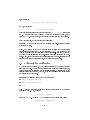
both methods either timed out or ran out of test terms.
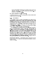
Zooming or no zooming?
The scatterplot in gure 1 below shows that the
use of zooming as a way to select test terms signicantly increases the ratio of
classied problems.
28
1000
14
111
RZ
100
10
1
1
10
100
R
The horizontal axis represents the method R, while the vertical axis corresponds
to its zoomed counterpart, RZ. We note that, while some dozen problems were
solved by both methods, there are a total of 111 problems along the 900 mark
of method R, which were solved by the zoomed version alone. Only 14 problems
were solved by R alone.
The results indicate that it is in most cases preferrable to use the zoom
feature. Only in a few cases did the plain R method succeed when the zoomed
version did not. Still, it may be of value try the plain R method when RZ has
failed. The two methods together classied just over 44% of the total number
of problems that were successfully classied by Innox.
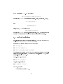
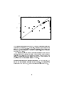
Limiting predicates or no limiting predicates?
In the gure below, we
see how the use of limiting predicates aects the result.
The horizontal axis
corresponds to the method RZ, while the vertical axis corresponds to RPZ.
29
1000
1000
127
216
RPZ
100
10
1
1
10
100
1000
RZ
A number of crosses are gathered around the diagonal line, indicating that the
performances of both methods were very similar on the problems that both
methods were able to solve.
Even more interesting are the crosses gathered
along the 900 second mark of both methods. We see that 127 problems were
classied by RZ but not by RPZ, and 216 problems were classied by RPZ but
not RZ. This shows that the two methods complement each other very well and
should ideally be combined. RPZ performed somewhat better, with a total of
235 classied problems, compared to RZ, which classied 146.
Together, the
two methods account for almost 93% of the total number of classied problems.
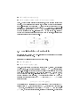
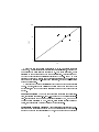
Injective and non-surjective or non-injective and surjective?
In the
gure below, we compare the results of the method that searches for terms that
are injective and non-surjective with the results of the method that searches for
non-injecitve and surjective terms. We look at the zoomed version of both methods. The horizontal axis corresponds to RZ, while the vertical axis corresponds
to SNIZ.
30
1000
140
100
SNIZ
5
10
1
1
10
100
RZ
We see that very few problems were solved by SNIZ. One reason for this is
that in RZ, we consider all reexive predicates as equality relation, while in SNIZ
we are limited to using standard equality (=). With fewer test cases, we are
less likely to come across a term that ts our description. Another reason may
be that the test problems are initially constructed by people. It may be more
intuitive to deal with a certain kind of functions (injective and non-surjective)
rather than the reverse (non-injective and surjective), and thus these functions
occur more frequently.
We conclude by the poor overall results that the SNIZ method is not practical
to use.
However, since SNIZ classies 5 problems for which all of the other
methods fail, it may be worthwhile to investigate ways in which to improve this
method.
Reexive predicates
The added use of reexive predicates as equality rela-
tion, as explained in sections 3.3. and 4.2.3, has shown to be a useful generalisation. It accounts for 41 out of the 146 problems classied by RZ, and 13 out of
the 235 problems classifed by RPZ. However, since regular equality performed
better, it should ideally be tested before any other predicates.
Existentially quantied variables
Using existential quantication to gen-
erate terms and predicates has proved to be of major signicance to the results.
In 104 out of the 146 problems classied by RZ, and 219 out of the 235 problems
31
1000
classied by RPZ, the identied terms and/or predicates include variables that
are existentially quantied.
Term depth
Out of all of the 390 classied problems, 100% of the identied
terms and predicates had depth 1. This does not exclude the possibility of there
being terms or predicates of larger depths that possess the desired properties.
These may exist, however they are much more dicult to nd.
5.3.3 Time-outs
Innox has three dierent time-out settings. The settings that are most suitable
highly depend on the nature of the problem and the global time-out.
The global time-out setting
The global time-out should ideally be as long
as possible. In our test results, the majority of the identied terms were found
in the time interval of 100 and 500 seconds, with an E limit of 2 seconds. Thus,
a time-out of at least 10 minutes per method is recommended. This should of
course be adjusted according to the time-out settings of E and Paradox.
E time-out setting
Naturally, a longer time-out for E means that it is more
likely to be able to prove our conjectures. However, it may also mean that there
won't be enough time to go through all of the tests. The E time-out should be
set in accordance with the global time-out and the size of the problem.
Paradox time-out setting
Using the zoom feature requires a time-out set-
ting for Paradox. In our tests, we used a time-out of 2 seconds, which our results
indicate is a reasonable limit. This is also the time limit used as default. With
a longer limit, we can decrease the risks of the zoomed problem having a nite
model which was not found by Paradox in the given time limit. However, with a
longer limit, there is the risk of global time-out before the zooming has nished
and any terms have been tested.
5.3.4 The less successful methods
The four methods R, RZ, RPZ and SNIZ together classify all of the in total
390 problems classied in our tests. A number of variations on these methods
were tested, but these did not add to the overall result. These include the use
of generation of terms and predicates up to a given depth. Our tests indicate
that if there exist terms with the desired properties, these are often syntactically
present in the problem. The generation of terms also yields a large number of
test cases, often too many to process before the time-out.
Another less successful attempt was to combine the limiting predicates by
conjunction, disjunction and negation.
q(X)
would yield the new predicates
For example, the predicates
p ∧ q , p ∨ q ,¬p
be used in addition to the plain limiting predicates.
32
and
¬q.
p(X)and
These would then
There are innitely many ways to generate terms and predicates to test. If
we haven't found a term with the desired properties at the lower term-depths,
the chances of generating the right term - if it exists - are just too slim.
5.4 Testing
During the implementation phase, Innox was continuously tested on 737 problems known to be nitely satisable to ensure that the program does not wrongly
infer the non-existence of nite models for these problems. While the correctness of the methods has been proved, the testing helped to locate bugs in the
code, such as misplaced parentheses that changed the intended quantication
scope of variables.
33
Chapter 6
Future work
Since we are dealing with a semi-decidable problem, the perfect algorithm for
proving nite unsatisability will never be invented. On the other hand, this
means that there are innitely many opportunities to improve the results, either
by enhancing the methods we have, or by inventing new ones.
6.1 Rene the methods
Perhaps the simplest way to improve our methods is to rene the techniques of
term/predicate selection. The more terms we have to test, the more likely it is
that one of them has the desired property. Since the running time is generally
bounded with a time-out, it is equally important to rule out the terms that for
various reasons are unnecessary to test. The relationship between the size of the
problem and the required global and local time-outs is something that should
be analysed in order to achieve the best possible results.
6.1.1 Selection of terms and predicates
The selection of test terms and predicates is of great importance to the result.
It is thus important to decide what terms are meaningful to test and what
limitations we should make to reduce the search space.
What to include
At present, terms and predicates are selected based on
those syntactically present in the problem.
This has proved to work well for
many problems, however it may also be of value to introduce new terms. By the
use of skolemization, existential quantiers are replaced with skolem functions,
which may be used as new test terms. If we can nd a function
r,
f
such that
∀Y : ∃X : r(f (X), Y )
i.e.
f
is surjective with respect to
r,
then we can add the axiom
34
and a relation
∀Y : r(f (g(Y ), Y )
to the theory, for a new function symbol
g,
for injective and non-surjective functions on
and use the method that searches
g.
One may also consider new ways of combining terms and predicates, and
analyse what combinations are meaningful to test. The generation of new limiting predicates by the use of conjunction, disjunction and negation has been
tested without major success. It would be interesting to look into other ways in
which to create limiting predicates. For example, one may introduce a predicate
for each function we test, that is true for an element i the function is injective
in that element.
What to exclude
When considering a problem of larger size, there may not
be enough time to test all the combinations of terms and predicates. The use
of zooming has helped in many of these cases, by focusing on a smaller part
of the problem where a nite model cannot be found.
But, as we have seen,
zooming does not work for all problems. In fact, it never will, since this would
imply the decidability of a semi-decidable problem. Still, further renement of
the zooming procedure could lead to even better results. One possible way to
improve the performance of zooming is to remember what axioms cannot be
removed without making the model nite.
not need
For example, if we start with the
{A, B, C, D} , and nd that {B, C, D}
to remove A in future steps.
axiom set
has a nite model, then we do
In order to reduce test terms further, it would also be of great value to
investigate what kind of terms are meaningful to test, in terms of term depth and
other attributes. As an example, it is meaningful to test the term
for injectivity only if both
g(X)
and
h(X)
f (g(X), h(X))
are injective.
6.1.2 Find the perfect time-out
A very important question is how to balance the global and local time-outs.
Ideally, the global time-out would be unlimited, and the local time-outs set to
as long as possible.
Since this is generally not practical, we must adjust the
local time-outs to match the size of the problem and the time we are willing to
wait for a result. Finding the best balance requires a lot of experimentation, but
signicant improvements to performance can be made by tuning the parameters
correctly.
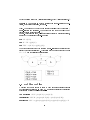
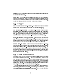
6.1.3 Other variatons
We have seen how we can weaken the constraints on the terms by the use of limiting predicates. Another alternative is to consider terms that are injective in all
but a limited number of elements, and adjust the constraint of non-surjectivity
accordingly.
35
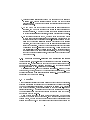
If a function f maps any n elements to k elements and is injective in all other
elements, where n >= k, and at least (n-k) + 1 elements in the codomain are
uncovered by the function, then the domain must be innite, as illustrated by
the pictures below.
With four elements that are mapped to two elements, and three elements
not covered by the function, we must introduce a fth element to the domain,
which must be mapped to a sixth elemement, and so on, given that the function
is injective in all other elements.
Here, three elements are mapped to a single element. With three elements
not covered by the function, we must introduce a fourth element to the domain,
which in turn must be mapped to a fth element, given that all elements except
the rst three map to dierent elements.
6.2 Develop new methods
There are many properties that a problem may possess which imply innity of
any of its models.
By exploring such properties and nding ways to express
them in a way that can be understood by a rst-order theorem prover, we can
extend Innox with new methods.
An example of a property that can be used to show innity of models is this:
if there for any model of a problem exists a smaller model of the same
problem, then all models must be innite.
The proof is simple. If the problem has nite models, then there must exist
a smallest model. For this model, the statement is contradictory.
To be able to express this property in rst-order logic, we need to use some
tricks to avoid quantication over models.
A non-surjective function can be
used to shrink a model, by applying it to each entry in each function table.
36
This particular method has been implemented and evaluated without major
success, which is why it is not yet a part of Innox. It may, however be worth
looking into alternative ways to implement this method.
Another example is the existence of a relation
r, that is irreexive, transitive
and serial, i.e.
1.
∀X : ¬r(X, X)
2.
∀X, Y : r(X, Y ) ∧ r(Y, Z) =⇒ r(X, Z)
3.
∀X : ∃Y : r(X, Y )
Given that the domain contains at least one element, say
a1 ,
these axioms yield
an innite sequence of unique elements:
a2 , such that r(a1 , a2 ). In the same way,
a(i+1) for every element ai , such that r(ai , a(i+1) ). By
r(ai , aj ), which by axiom 1 implies ai 6= aj for all i, j such that
By axiom 3, there exists an element,
there exists an element
axiom 2, we get
i < j.
This sequence of elements can thus not be nite: Suppose there is a last
ak . By axiom 3, there exists an element a(k+1) such that r(ak , a(k+1) ),
ai 6= a(k+1) for all ai such that 1 ≤ i ≤ k . Thus, every element of the
element,
and
sequence gives rise to a new, unique element.
This method has been implemented, but not yet evaluated. Evaluation and
investigation of possible generalisations of this method is left as future work.
6.3 Evaluation
A thorough evaluation of the performance of the dierent methods and time-out
settings is crucial to be able to create improved future versions of Innox, both
to adjust parameters, and to get an insight in what can be improved upon. A
useful improvement that could be made with this knowledge is to automatically
base the local time-outs on the given global time-out and problem size. The aim
is to let Innox automatically decide the best approach for a given problem, and
thus save the user having to go through each method one by one.
6.4 Other uses
To simplify the addition of new properties to Innox is something that should
be considered in future implementations. This could be further generalised to
allow the user to search for terms or predicates with any type of property. One
way to do this could be to provide a specic language to let the users program
these properties themselves.
37
Chapter 7
Conclusions
We have introduced Innox, a new tool that can be used to disprove the existence
of nite models of rst-order theories.
Innox is especially well suited as a
complement to nite model nders; by proving that a nite model cannot exist,
it is no longer necessary to search for one.
Disproving the existence of nite models
We have demonstrated how
terms that are injective and non-surjective, or non-injective and surjective imply
the non-existence of nite models. Innox automates the process of nding such
terms. In the search for terms with the desired properties, we focus on terms
that are syntactically present in the theory.
Existential quantication to create test terms
With the use of existen-
tial quantication, variables are instantiated by a constant in order to create new
test terms of the desired arity. This addition has improved the results considerably. A majority of the identied terms in our test problems are existentially
quantied.
Zooming to reduce test terms
By the use of zooming, we focus on a smaller
part of the problem where a nite model cannot be found, and thus reduce the
number of terms to test. Zooming works very well for a lot of problems, while
it fails miserably for some others. A major reason for this is that there is no
guarantee that we zoom in to the right part of the problem. It is possible that
we zoom in to a subproblem for which none of our methods work, while another
part of the problem holds a function of the kind we are looking for. Another
possibility is that we zoom in to a subproblem that does in fact have a nite
model. The zooming feature relies on the assumption that if no nite model has
been found within a set time limit, then no nite model exists.
Generalising the properties
By generalising the properties that we look
for, we are able to detect more terms that imply the non-existence of a nite
38
model.
Reexive relations can be used as a complement to regular equality when
dening the property of injectivity and non-surjectivity.
For surjectivity and
non-injectivity we need stronger constraints on the relation, which is why only
equality is used for this property at present.
With limiting predicates, we can identify terms for which the given property
is valid on an (innite) subset of the domain, as dened by the predicate. In
this way we can identify terms that do not have the desired property when the
full domain is considered.
Pros and cons
With the above generalisations, we get an increased number
of tests to perform; one for each combination of terms, reexive predicates and
limiting predicates. More test cases increases the likelihood of a term with the
desired property being among them.
When using a global time-out, this can
also be a disadvantage, since there might not be enough time to go through all
combinations.
Our results indicate that the use of limiting predicates should
be used as a complement to the general method, since they are both able to
classify some problems that the other method cannot.
The results
Innox has classied over 30% of the standard rst-order logic
test problems as nitely unsatisable. Many of these problems have never before
been solved (nor classied) by an automated system. Since this classication
has never been done automatically before, the new problem status denition
FinitelyUnsatisable has been added to the TPTP libary of standard problems
for automated theorem provers.
39
Bibliography
[1] J. Bruggeman, J. Kamps, M. Masuch, B. O'Nuallain, Automated Reasoning
for Theory-Building in the Social Sciences, CCSOM Working Paper 96-144,
1996.
[2] A. Church, A Note on the Entscheidungsproblem, Journal of Symbolic
Logic, 1, pp. 40-41, 1936.
[3] K. Claessen, N. Sörensson, New Techniques that Improve MACE-style
Finite Model Finding, In Proc. of Workshop on Model Computation
(MODEL), 2003.
[4] S. Cook, The Complexity of Theorem Proving Procedures, Proc. 3rd ACM
Symp. on the Theory of Computing, ACM, pp. 151-158, 1971.
[5] N. Eén, N. Sörensson, The MiniSat Page, http://www.minisat.se.
[6] B. Han, S. Lee, H. Yang, A Model-Based Diagnosis System for Identifying
Faulty Components In Digital Circuits, Appl. Intell., 10(1), pp. 37-52, 1999.
[7] M. Kaufmann, J. Strother Moore, Some Key Research Problems in Auto-
mated Theorem Proving for Hardware and Software Verication, Spanish
Royal Academy of Science (RACSAM), 98(1), pp. 181-196, 2004.
[8] P. Lucas, The Representation of Medical Reasoning Models in Resolution-
Based Theorem Provers, Articial Intelligence in Medicine, 5(5), pp. 395414, 1993.
[9] W. McCune, Prover9 and Mace, http://www.cs.unm.edu/~mccune/mace4
[10] W. McCune, Solution of the Robbins Problem, Journal of Automated Reasoning, 19(3), pp. 263-276, 1997.
[11] P. Norvig, S. Russell, Articial Intelligence - A Modern Approach, Prentice
Hall, 2003.
[12] A. Riazanov, A. Voronkov, Vampire, Proc. CADE-16, LNAI 1632, 1999.
[13] A. Robinson, A. Voronkov, Handbook of Automated Reasoning, MIT Press,
2001.
40
[14] J.A. Robinson, A Machine-Oriented Logic Based on the Resolution Prin-
ciple, Journal of the ACM (JACM), 12(1), pp. 23-41, 1965.
[15] S. Schulz, The E Equational Theorem Prover, http://www4.informatik.tu-
muenchen.de/~schulz/WORK/eprover
[16] R. M. Smullyan, First-Order Logic, Courier Dover Publications, 1995.
[17] G. Sutclie, C. Suttner, Evaluating General Purpose Automated Theorem
Systems, Articial Intelligence, 131:39-54, 2001.
[18] G. Sutclie, C. Suttner, The TPTP Problem Library for Automated Theo-
rem Proving, http://www.cs.miami.edu/~tptp
[19] G. Sutclie, C. Suttner, The TSTP Solution Library for Automated Theo-
rem Proving, http://www.cs.miami.edu/~tptp/TSTP
[20] G.
Sutclie,
C.
TPTP
Suttner,
Format
for
Problems,
http://www.cs.miami.edu/~tptp/TPTP/QuickGuide/Problems
[21] J. Vännänen, A Short Course on Finite Model Theory, Department of
Mathematics, University of Helsinki, 1994.
[22] C. Weidenbach et al., The Spass Homepage, Max-Planck-Institut Informatik, http://www.spass-prover.org, 2008.
[23] H. Zhang, J. Zhang, SEM: a System for Enumerating Models, In Proc. of
International Joint Conference on Articial Intelligence (IJCAI'95), 1995.
41
Appendix A
Using Innox
Requirements
Innox requires installations of E [15] and Paradox [3]. These
must either be located in the working directory, or added to the PATH variable.
The problems must be expressed in the TPTP-format [20].
Temporary les
During execution, Innox creates temporary les, which are
stored in the temp directory. The temp directory is not removed after execution,
but all of the temporary les created by that program run are deleted, given
that the program terminates normally.
Example use
The following command will run Innox on the le problem.tptp,
using reexive relations and limiting predicates, and 4 seconds time-out for E
and Paradox, and a global time-out of 10 minutes.
innox problem.tptp -r -p -elimit=4 -plimit=4 -timeout=600
Output
In the case of time-out, or if Innox runs out of terms to test,
# RESULT: GaveUp
is printed to stdout. If a term of the desired property is found,
#RESULT: FinitelyUnsatisable is printed, together with the found term, and relation and predicate, where
applicable.
42
Flags
-v
print details of the progress of the program to stdout
-lelist=<lename> run program on all problems listed in the given le
-dir=<directoryname> run program on all problems found in the given directory
-o=<lename> print results to the given le
-elimit=<n>
time limit in seconds for each call to E (default=2)
-plimit=<p>
time limit in seconds for each call to paradox (default=2)
-timeout=<n>
timeout in seconds (default=3600)
-r
use all reexive predicates as equality relation
-p
use limiting predicates, can be used in combination with:
-and
use pairwise conjunction of limiting predicates
-or
use pairwise disjunction of limiting predicates
-not
use negation of limiting predicates
-g=<n> generate all terms of depth n from all function symbols present in
the problem
-zoom
use zoom feature to select terms
-ino
search for injective and non-surjective terms (default)
-oni
search for non-injective and surjective terms. NOTE: invalidates the
-r ag
-m2
nd a smaller model by applying a non-surjective function
-sr
search for a relation that is serial, irreexive and transitive
-term=<t> test the the term t only
43