Download EASiTool - User Manual - V2.0

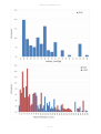
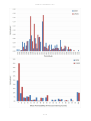
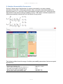
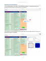
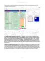
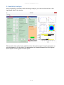
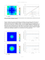
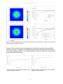
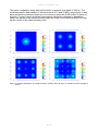
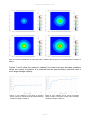
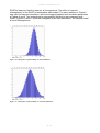
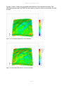
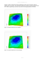
EASiTool
V2.0
User Manual
EASiTool - User Manual - V2.0
Table of Contents
Introduction ............................................................................................................... 3
What's New? .......................................................................................................... 3
Getting Started .......................................................................................................... 4
System Requirements ............................................................................................. 4
Installment ............................................................................................................ 4
Input Parameters ....................................................................................................... 8
1. Reservoir Parameters ......................................................................................... 8
2. Relative Permeability Parameters ...................................................................... 13
3. Simulation Parameters ...................................................................................... 14
4. NPV Analysis .................................................................................................... 18
Running the Simulation............................................................................................. 19
Outputs ................................................................................................................... 20
1. Optimal Constant-Injection Rate........................................................................ 20
2. Sensitivity Analysis ........................................................................................... 23
Examples and Verifications........................................................................................ 24
References............................................................................................................... 34
Contacts .................................................................................................................. 35
2 / 35
EASiTool - User Manual - V2.0
Introduction
Welcome to the second released version of EASiTool (Enhanced Analytical Simulation
Tool), developed for CO2 storage-capacity estimation and uncertainty quantification.
This User Manual will help you install and use EASiTool.
EASiTool is intended to help users achieve a fast, reliable, science-based estimate of
storage capacity for any geological formation containing brine. EASiTool, which provides
strategies for optimizing a project's net present value (NPV), offers three major features:



An advanced, closed-form analytical solution for pressure-buildup calculations used to
estimate both injectivity and reservoir-scale pressure elevation, in both closed- and
open-boundary aquifers (version 1.1)
A simple geomechanical model coupled with a base model to evaluate and avoid the
possibility of fracturing reservoir rocks by injecting cold, supercritical CO2 into hot
formations, which can cause rock deformation (version 2.0)
An active reservoir-management system throughout the brine-extraction process
(version 3.0, to be released in 2016)
Disclaimer
This project is funded by the U.S. Department of Energy (DE-FE0009301).
This report was prepared as an account of work sponsored by an agency of the United
States Government. Neither the United States Government nor any agency thereof, nor
any of their employees, makes any warranty, express or implied, or assumes any legal
liability or responsibility for the accuracy, completeness, or usefulness of any information,
apparatus, product, or process disclosed, or represents that its use would not infringe
privately owned rights. Reference herein to any specific commercial product, process, or
service by trade name, trademark, manufacturer, or otherwise does not necessarily
constitute or imply its endorsement, recommendation, or favoring by the United States
Government or any agency thereof. The views and opinions of authors expressed herein
do not necessarily state or reflect those of the United States Government or any agency
thereof.
Further Information
This software has been developed using MATLAB R2015a.
What's New?
Important changes in EASiTool V2.0:



The program platform has been transferred from GoldSim to MATLAB.
A simple geomechanical model has been coupled with the base model to evaluate the
maximum injection pressure internally. User still has the option to enter the maximum
injection pressure manually.
Graphical outputs have been added to the results. Outputs include capacity vs.
number of injection wells, NPV vs. number of injection wells, extend of CO 2 plume in
injection area, optimal injection rate of wells, and tornado chart for sensitivity analysis.
3 / 35
EASiTool - User Manual - V2.0
Getting Started
This section has information on system requirements and installment for EASiTool.
System Requirements
EASiTool is a Windows application. Windows Vista, Windows 7 (either 32-bit or 64-bit
versions), or Windows 8 are the recommended operating systems. Windows XP (SP3) is
also supported.
You must have administrative privileges on the system. You need a minimum of 600 MB
disk space during the installation process. 16-bit color depth is required (32-bit
recommended).
Installment
Once you download the install file from EASiTool website, double-click it to start the
installment. Click "Next" once you see the window below:
4 / 35
EASiTool - User Manual - V2.0
Determine the destination folder. If you don't want to change the location where the
installation folder will be saved, click "Next":
MATLAB Compiler Runtime is required. Determine the destination folder. If you don't
want to change the location where the installation folder will be saved, click "Next":
5 / 35
EASiTool - User Manual - V2.0
Select "Yes" to accept the terms of license agreement. Then, click "Next":
Click "Install" to begin the installation:
6 / 35
EASiTool - User Manual - V2.0
Once the installation is completed (this may take a few minutes), you will see the window
below. Click "Finish":
Now you are ready to use EASiTool software by simply double-clicking on the EASiTool
icon.
7 / 35
EASiTool - User Manual - V2.0
Input Parameters
Section 1 has information on the input data required to run the program.
1. Reservoir Parameters
Necessary input for reservoir parameters includes in situ pressure (MPa), temperature
(C), salinity of the formation brine (mol/kg), thickness (m), porosity, permeability (mD),
rock compressibility (1/Pa), reservoir area (km^2), basin area (km^2), and boundary
condition, as shown in Section 1 at the top left-hand side of the input screen.
Note: Currently we only accept one set of fixed units; if units are different from what is
shown on the interface, they have to be converted first.
Reservoir Area (km^2): A reservoir is a part of the basin in which injectors are
distributed. In the current version, we assume that reservoirs do not include detailed
structures or dip angles. We also assume that reservoirs are square and placed at the
center of the basins.
Basin Area (km^2): A basin is the whole areal extent of the storage formation in which
the reservoir of our interest is located. In the current version, we assume that basins do
not include detailed structures or dip angles. We also assume that basins are square.
Basin area should be bigger or equal to reservoir area.
Boundary Condition: Using the drop-down menu, select either an "open" or a "closed"
boundary condition. (In the current version of EASiTool, the selected boundary condition
will be enforced on all four sides of the basin.) A reservoir can be considered open as
long as the pressure change has not reached the boundaries. In an industrial-scale
injection operation, it is expected that the pressure effect reaches the boundaries of the
basin at late times.
8 / 35
EASiTool - User Manual - V2.0
Note: EASiTool is designed to do the calculations for multiple scenarios where the
number of wells increases from 1 to 400 in square numbers (11, 22, 33,
44, ..., 2020). In each scenario, wells are equally spaced over the reservoir area.
For example, well distribution for a 22 pattern is as shown below:
The following table shows the range of parameters that are accepted by EASiTool:
Initial Pressure
Initial Temperature
Thickness
Salinity
Porosity
Permeability
Rock Compressibility
Reservoir Area
≤ 60.0 MPa
≤ 300.0 ˚C
≥ 0.1 m
≥ 0.0 mol/kg and ≤ 6.0 mol/kg
≥ 0.0 and ≤ 0.9999
≥ 0.0 mD
≤ 1.0E-08 1/Pa
≤ Basin Area
The following six figures show the range and frequency of some reservoir parameters,
based on two data sets prepared by DOE and USGS:
9 / 35
EASiTool - User Manual - V2.0
10 / 35
EASiTool - User Manual - V2.0
11 / 35
EASiTool - User Manual - V2.0
12 / 35
EASiTool - User Manual - V2.0
2. Relative Permeability Parameters
Section 2 allows input of parameters for relative permeability, including residual
saturation of brine (Sar), critical gas saturation (Sgc), end-point relative permeability for
aqueous phase (kra0), end-point relative permeability for gas phase (krg0), and power-law
exponents for the aqueous and gas phases m and n. This section includes equations for
relative permeability calculations from the Brooks-Corey model:
The following table shows the range of relative permeability parameters that are accepted
by EASiTool:
≥ 0.0 and ≤ 0.9999
≥ 0.0 and ≤ 0.9999
≤ 1.0
≤ 1.0
≥ 0.0 and ≤ 1.0
≥ 0.0 and ≤ 1.0
Residual water saturation, Sar
Residual gas saturation, Sgr
Water relative permeability Corey exponent, m
Gas relative permeability Corey exponent, n
Water end-point relative permeability, Kra0
Gas end-point relative permeability, Krg0
13 / 35
EASiTool - User Manual - V2.0
Typical range of relative permeability parameters based on data published in literature is
listed in the table below:
0.2 – 0.6
0.1 – 0.35
1.5 – 4.0
1.5 – 4.0
1.0
0.1 – 0.6
Residual water saturation, Sar
Residual gas saturation, Sgr
Water relative permeability Corey exponent, m
Gas relative permeability Corey exponent, n
Water end-point relative permeability, Kra0
Gas end-point relative permeability, Krg0
3. Simulation Parameters
Section 3 has three input parameters for simulation: simulation time (years), injection well
radius (m), and maximum injection pressure (MPa).
The maximum acceptable injection well radius is 1.0 m. The maximum injection pressure
should also be larger than the initial pressure and smaller than three times the initial
pressure.
14 / 35
EASiTool - User Manual - V2.0
Geomechanics Package
The new version of EASiTool can calculate the maximum allowable injection pressure
internally from the reservoir properties. To include the geomechanics, check "Estimate
Max Injection Pressure Internally". Then, in the new boxes, provide the following
properties to estimate the maximum injection pressure:
Density of Porous Media () [kg/m3]: Density of porous media can be calculated as
=d (1-) +  f, where  is porosity; f is fluid density; and d is dried density of the
matrix.
Total Stress Ratio (V/H): The ratio of vertical to horizontal stress (1/Kh). Kh is coefficient
of lateral stress or lateral stress ratio σh/σv.
Biot Coefficient (): The effective-stress principle is of fundamental significance in soil
and rock mechanics and is defined as σeff = σc - σp, where σc and σp are the total
confining stress and fluid pore pressure, respectively. However, in fluid-saturated rocks,
Terzaghi’s effective-stress principle may not be always valid. The Biot coefficient  (other
than unity) was suggested to modify the effective-stress principle (Biot, 1941), which is
given by σeff = σc -  σp. The Biot coefficient  is a property of a solid constituent only.
The existence of the Biot coefficient suggests that pore pressure modifies not only
effective normal stresses but also effective shear stresses.
Note:  ≤ α ≤ 1, where  is porosity; α will be near its upper limit for soil-like materials.
15 / 35
EASiTool - User Manual - V2.0
Poisson's Ratio (): An elastic constant that is a measure of the compressibility of
material perpendicular to applied stress, i.e., the ratio of latitudinal to longitudinal strain
(0<<0.5). Poisson's ratio can be expressed in terms of properties that can be measured
in the field, including velocities of P-waves and S-waves. Approximate Poisson's ratio for
carbonate rocks is ~ 0.3; for sandstones, ~ 0.2; and for shale, above 0.3.
Coefficient of Thermal Expansion [1/K]: The coefficient of thermal expansion
describes how the size of an object changes with a change in temperature. Specifically, it
measures the fractional change in size per degree change in temperature at a constant
pressure.
Bottom-Hole Temperature Drop [1/K]: The temperature difference between the
formation and the injected fluid (CO2) at the bottom of the well bore. The fluid
temperature is lower than the bottom-hole static temperature. The corresponding
temperature difference causes thermal stresses in the formation and affects the Max
Injection Pressure.
Young's Modulus (E) [Pa]: Young's modulus, also known as the tensile modulus,
modulus of elasticity, or elastic modulus, is defined as the ratio of the stress (force per
unit area) along an axis to the strain (ratio of deformation over initial length) along that
axis in the range of linear behavior of the material.
Depth [m]: Depth of the fluid injection (depth of perforation zone).
Estimated Max Injection Pressure [MPa]: Pressure above which injection of fluids will
cause the rock formation to fracture hydraulically. Reactivation of preexisting fracture
planes via shear slip is likely to occur prior to other types of geomechanical failures in
most cases. The Mohr-Coulomb shear failures criterion for the maximum pressure limit
is expressed as
,
where is shear stress, is normal stress acting on a preexisting fracture plane,
cohesion, and is the coefficient of friction.
Then, the
is
,
where , , and are major principal stress, minor principal stress, and angle with
reference to minor principal stress, respectively.
16 / 35
is
EASiTool - User Manual - V2.0
Sensitivity Analysis
EASiTool currently can do sensitivity analysis on any combination of initial reservoir
pressure, temperature, salinity, thickness, porosity, permeability, rock compressibility,
and relative permeability parameters. To include the sensitivity analysis of any of these
parameters, check "Sensitivity Analysis (Slow)". Then, in the new boxes, provide the
percentage of the variation of the parameters for sampling.
The one-parameter-at-a-time method is used for sampling in this version of EASiTool. In
this method, information about the effect of a parameter is gained by varying only one
parameter at a time. Because this procedure is repeated in turn for all parameters to be
studied, running sensitivity analysis simulations may take a few minutes to complete.
Sensitivity-variation value should be less than 100% and greater than 0%.
17 / 35
EASiTool - User Manual - V2.0
4. NPV Analysis
Section 4 provides the option to conduct a very simple net present value (NPV) analysis
along with the simulation. Here, you can input parameters such as Drilling Cost (million
$/well), Operation Cost (kilo $/well/year), Monitoring Cost (kilo $/year/km2), and Tax
Credit ($/tonne):
The following table shows the range of NPV parameters that are accepted by EASiTool:
Drilling Cost
Operation Cost
Monitoring Cost
Tax Credit
≥ 0.0001 million $/well
≥ 0.0001 kilo $/well/year
≥ 0.0001 kilo $/year/km 2
≥ 0.0 $/tonne
18 / 35
EASiTool - User Manual - V2.0
Running the Simulation
To run the simulation, click "Run" in the EASiTool interface. A progress bar pops up,
showing the percentage of the progress in calculations:
The simulation results will appear on the right side of the controller window to inform you
that the simulation is complete:
19 / 35
EASiTool - User Manual - V2.0
Outputs
This section provides information on how to evaluate the outputs of EASiTool.
1. Optimal Constant-Injection Rate
After completing a simulation, you can see the results on the right hand side of the
window:
The results include the "Storage Capacity (MtCO2)," "NPV ($M)," "CO2 Plume Extension
(Graphical map view)," and "Well Injection Rate (tonne/day)."
In the orange "Results Controls" box, check the "Export Image Files (Slow)" to save the
graphical results at the location where the installation folder was installed.
20 / 35
EASiTool - User Manual - V2.0
To look at the values, press the "Data Cursor" icon in the upper tab:
Then, click on the "Well Injection Rate" contour to see the value and coordinates of each
well:
21 / 35
EASiTool - User Manual - V2.0
The number of injection wells can be changed by clicking on the drop-down menu for
"Number of Injection Wells":
The total CO2 storage capacity and NPV of the simulated scenario based on number of
injection wells can be viewed by clicking on the circles of the "Capacity" and "NPV" plots.
The "Zoom In" and "Zoom Out" options can be used to focus on the output figures.
To interpret the results from figures: For example, for the scenario of a total of four
wells (refer to the drop-down menu in the "5-Result Controls: Number of Injection Wells"
section), click on the location of all four wells on the "Well Injection Rate" plot. The popup boxes provide the injection rate (tonne/day) corresponding to these four wells: that is,
509.8 tonne/day for the #1 well, 509.8 tonne/day for the #2 well, 509.8 tonne/day for the
#3 well, and 509.8 tonne/day for the #4 well. The rate of all four wells is similar as a result
of symmetry.
Optimal constant-injection rate: This procedure guarantees that nonidentical constantinjection rates are calculated optimally at each well to meet the maximum pressure limit
at the end of simulation time. For example, if the pressure limit is selected to be 20 MPa
for a 20-year simulation, then the program will calculate injection rates for all wells so that
the bottom-hole pressure of the wells will increase by 20 MPa at the end of 20 years.
22 / 35
EASiTool - User Manual - V2.0
2. Sensitivity Analysis
After completing a simulation with sensitivity analysis, you can see the results on the
right-hand side of the window:
The tornado chart on the lower right-hand side shows the impact of each parameter on
the total capacity. On this chart, the parameters are listed downward from the highest
direct impact to the highest inverse impact.
23 / 35
EASiTool - User Manual - V2.0
Examples and Verifications
Table 1 summarizes the input for the EASiTool template. The aquifer is located at a
depth of 1000 m. In this study, the problem was solved for closed and open boundary
conditions. The basin area is the same as the reservoir area for the case of the closed
boundary condition. The basin area is 10,000 km2 for the case of the open boundary
condition.
Table 1: Template Input
Initial pressure, MPa
Initial temperature, ˚C
Thickness, m
Salinity, kg/mol
Porosity
Permeability, mD
Rock compressibility, 1/Pa
Reservoir area, km2
Basin area, km2
Boundary Condition
10
40
100
0
0.2
100
5.0E-10
100
100 or 10000
Closed or Open
Table 2 summarizes the relative permeability parameters used in the Brooks-Corey
model for a two-phase flow of gas and aqueous phases.
Table 2: Relative Permeability Parameters for Brooks-Corey Model
0.5
Residual water saturation,
0.1
Residual gas saturation,
3.0
3.0
1.0
0.3
Water exponent,
Gas exponent,
Water end-point relative permeability,
Gas end-point relative permeability,
Table 3 shows the simulation parameters. It is assumed that the maximum allowable
pressure in the reservoir should not be above 20 MPa after 20 years of injection with
constant rates.
Table 3: Simulation Parameters
Simulation time, year
Injection well radius, m
Maximum injection pressure, MPa
20
0.1
20
24 / 35
EASiTool - User Manual - V2.0
The basin models were prepared for numerical simulation using CMG-GEM for both
boundary conditions. The injection rates calculated by EASiTool were used in numerical
simulation to compare the analytical and numerical results. Figure 1 shows the pressure
distributions throughout the reservoir and bottom-hole pressures of all wells after 20
years of injection using 1, 4, 9, and 16 injectors. The injection rates were calculated using
the closed boundary condition of EASiTool. The color legend shows the range of
pressure throughout the reservoir at the time of 20 years. It is observed that the
maximum pressure in the reservoir is very close to the target pressure of 20 MPa. The
pressure distribution is more uniform by using more injectors. The bottom-hole pressure
of all wells is very similar throughout the injection period.
a)
1 well
b) 4 wells
c)
9 wells
25 / 35
EASiTool - User Manual - V2.0
d) 16 wells
Figure 1: Pressure distributions and bottom-hole pressures for the closed boundary condition after 20 years
of constant injection at depth of 1000 m.
Figure 2 shows the pressure distributions and bottom-hole pressures after 20 years of
injection using the open boundary condition. It is assumed that a 100 km 2 reservoir is
located at the center of a 10,000 km2 basin. There is a slight difference between the final
pressure from simulations and the final pressure of 20 MPa in EASiTool. This difference
decreases when more injectors are used. Also, the simulation results show that the effect
of pressure reaches the boundaries of the basin at the end of injection process. It means
that the open boundary condition is not accurate for a 20-year process.
a)
1 well
b) 4 wells
26 / 35
EASiTool - User Manual - V2.0
c)
9 wells
d) 16 wells
Figure 2: Pressure distributions and bottom-hole pressures for open boundary condition after 20 years of
constant injection at depth of 1000 m.
Figures 3 and 4 show the maximum capacity for closed and open boundary problems
versus the number of injectors. It is observed that the open boundary reservoirs have a
much larger storage capacity. The storage capacity of reservoirs becomes constant after
a specific number of injectors.
Figure 3: CO2 capacity for 20 years of injection
versus number of injectors using closed boundary
condition at depth of 1000 m.
Figure 4: CO2 capacity for 20 years of injection
versus number of injectors using open boundary
condition at depth of 1000 m.
27 / 35
EASiTool - User Manual - V2.0
The same comparative study was performed for a reservoir at a depth of 3000 m. The
initial temperature and pressure in this study were 90˚C and 30 MPa, respectively. It was
assumed that the maximum pressure in the reservoir would be 40 MPa after 20 years of
injection. Figures 5 and 6 show the final pressure distribution obtained by simulation.
Again, the results of the closed boundary case are closer to the results of EASiTool than
are the results of the open boundary case.
a)
1 well
b) 4 wells
c)
9 wells
d) 16 wells
Figure 5: Pressure distribution for closed boundary condition after 20 years of constant injection at depth of
3000 m.
28 / 35
EASiTool - User Manual - V2.0
a)
1 well
b) 4 wells
c)
9 wells
d) 16 wells
Figure 6: Pressure distribution for open boundary condition after 20 years of constant injection at depth of
3000 m.
Figures 7 and 8 show the maximum capacity for closed and open boundary problems
versus the number of injectors. It is observed that the open boundary reservoirs have a
much larger storage capacity.
Figure 7: CO2 capacity for 20 years of injection
versus number of injectors using closed boundary
condition at depth of 3000 m.
Figure 8: CO2 capacity for 20 years of injection
versus number of injectors using open boundary
condition at depth of 3000 m.
29 / 35
EASiTool - User Manual - V2.0
EASiTool assumes that the reservoir is square, flat, and horizontal. The effect of reservoir
shape and structure on the EASiTool estimations was studied. An anticline model was
used for reservoir simulation with the average properties of the reservoir used as input for
EASiTool. Estimated injection rates by EASiTool were also used as input for reservoir
simulation. Tables 4 and 5 show the average properties of the anticline reservoir and the
simulation parameters. Figure 9 shows the pressure distribution in the reservoir after 10
years of injection with 16 injectors. The simulation predicts the maximum pressure of
24.07 MPa, which is very close to the target pressure of 25 MPa.
Table 4: Properties of Anticline Reservoir
Reference pressure, MPa
Reference depth, m
Initial temperature, ˚C
Average thickness, m
Salinity, kg/mol
Porosity
Permeability, mD
Rock compressibility, 1/Pa
Reservoir area, km2
Basin area, km2
Boundary Condition
Table 5: Simulation Parameters
Simulation time, year
Injection well radius, m
Maximum injection pressure, MPa
16.55
1750
40
24.39
0
0.2
100
5.0E-10
42.87
42.87
Closed
20
0.1
25
Figure 9: Pressure distribution after 20 years of injection with 16 injectors.
30 / 35
EASiTool - User Manual - V2.0
EASiTool assumes that the reservoir is homogeneous. The effect of reservoir
heterogeneity on the EASiTool estimations was studied. The same anticline in Figure 9
was used for reservoir simulation, with the average properties and simulation parameters
of Tables 4 and 5. Two realizations for permeability distribution were prepared with
Petrel. Figures 10 and 11 show the histograms of the two realizations. The second model
is more heterogeneous.
Figure 10: Histogram of permeability for first realization.
Figure 11: Histogram of permeability for second realization.
31 / 35
EASiTool - User Manual - V2.0
Figures 12 and 13 show the permeability distributions of the respective models. The
estimated injection rates by EASiTool were used as input for reservoir simulation for both
models.
Figure 12: Permeability distribution for first realization.
Figure 13: Permeability distribution for second realization.
32 / 35
EASiTool - User Manual - V2.0
Figures 14 and 15 show the pressure distribution in the reservoir after 20 years of
injection with 16 injectors. The simulation predicts the maximum pressure of 25.07 and
25.51 MPa, respectively, which are very close to the target pressure of 25 MPa.
Figure 14: Pressure distribution for first realization.
Figure 15: Pressure distribution for second realization.
33 / 35
EASiTool - User Manual - V2.0
References
Azizi, E. and Cinar, Y., 2013, A new mathematical model for predicting CO2 injectivity, Energy Procedia, 37,
3250-3258.
Azizi, E. and Cinar, Y., 2013, Approximate analytical solutions for CO 2 injectivity into saline formations,
SPE Reservoir Evaluation & Engineering, 16(2), 123-133.
Bachu, S. and Bennion, B., 2008, "Effects of in-situ conditions on relative permeability characteristics of
CO2-brine systems", Environmental Geology, 54 (8), 1707-1722.
Duan, Z. and Sun, R., 2003, "An improved model calculating CO 2 solubility in pure water and aqueous
NaCl solutions from 273 to 533 K and from 0 to 2000 bar", Chemical Geology, 193, 257-271.
Hosseini, S.A., Mathias, S.A., and Javadpour, F., 2012, "Analytical model for CO 2 injection into brine
aquifers-containing residual CH4" Transport in Porous Media, 94, 795-815.
Kim, S., and Hosseini, S.A., 2014, "Geological CO2 storage: Incorporation of pore-pressure/stress coupling
and thermal effects to determine maximum sustainable pressure limit", Energy Procedia, 63, 3339-3346.
Kim, S., and Hosseini, S.A., 2014, "Above-zone pressure monitoring and geomechanical analyses for a
field-scale CO2 injection project in Cranfield, MS", Greenhouse Gases: Science and Technology, 4(1), 8198.
King, C.W., Gulen, G., Cohen, S.M., and Nunez-Lopez, V., 2013, "The system-wide economics of a carbon
dioxide capture, utilization, and storage network: Texas Gulf Coast with pure CO 2-EOR flood",
Environmental Research Letters, 8, 034030.
Mathias, S.A., Gluyas, J.G., Gonzalez Martinez de Miguel, G.J., Bryant, S.L., and Wilson, D., 2013, "On
relative permeability data uncertainty and CO2 injectivity estimation for brine aquifers", International Journal
of Greenhouse Gas Control, 12, 200-212.
Mathias, S.A., Gluyas, J.G., Gonzalez Martinez de Miguel, G.J., and Hosseini, S.A., 2011, "Role of partial
miscibility on pressure buildup due to constant rate injection of CO 2 into closed and open brine aquifers",
Water Resources Research, 47, W12525.
Spycher, N., Pruess, K., and Ennis-King, J., 2003, "CO2-H2O mixtures in the geological sequestration of
CO2. I. Assessment and calculation of mutual solubilities from 12 to 100C and up to 600 bar", Geochimica
et Cosmochimica Acta, 67(16), 3015-3031.
Tseng, P.-H. and Lee, T.-C., 1998, "Numerical evaluation of exponential integral: Theis well fuction
approximation", Journal of Hydrology, 205, 38-51.
U.S. Geological Survey, 2013, "National Assessment of Geologic Carbon Dioxide Storage Resources—
Data", http://pubs.usgs.gov/ds/774/.
Zeidouni, M., Pooladi-Darvish, M., and Keith, D., 2009, "Analytical solution to evaluate salt precipitation
during CO2 injection in saline aquifers", International Journal of Greenhouse Gas Control, 3, 600-611.
34 / 35
EASiTool - User Manual - V2.0
Contacts
Principle Investigator: Seyyed A. Hosseini
10100 Burnet Rd, Bldg. 130, Austin, TX 78758
Phone: +1 512-471-2360
Email: [email protected]
35 / 35