Download nitpick - Isabelle - Technische Universität München

b
le
l
e
a
Is
λ
Nitp
ick
∀
=
α
→
β
Picking Nits
A User’s Guide to Nitpick for Isabelle/HOL
Jasmin Christian Blanchette
Institut für Informatik, Technische Universität München
May 25, 2015
Contents
1 Introduction
2
2 Installation
3
3 First Steps
3.1 Propositional Logic . . . . . . . . . . . . . . .
3.2 Type Variables . . . . . . . . . . . . . . . . .
3.3 Constants . . . . . . . . . . . . . . . . . . . .
3.4 Skolemization . . . . . . . . . . . . . . . . . .
3.5 Natural Numbers and Integers . . . . . . . . .
3.6 Inductive Datatypes . . . . . . . . . . . . . .
3.7 Typedefs, Quotient Types, Records, Rationals,
3.8 Inductive and Coinductive Predicates . . . . .
3.9 Coinductive Datatypes . . . . . . . . . . . . .
1
. . . . . .
. . . . . .
. . . . . .
. . . . . .
. . . . . .
. . . . . .
and Reals
. . . . . .
. . . . . .
.
.
.
.
.
.
.
.
.
.
.
.
.
.
.
.
.
.
.
.
.
.
.
.
.
.
.
4
4
5
6
7
8
11
12
15
19
3.10 Boxing . . . . . . . . . . . . . . . . . . . . . . . . . . . . . . . 21
3.11 Scope Monotonicity . . . . . . . . . . . . . . . . . . . . . . . . 23
3.12 Inductive Properties . . . . . . . . . . . . . . . . . . . . . . . 25
4 Case Studies
27
4.1 A Context-Free Grammar . . . . . . . . . . . . . . . . . . . . 27
4.2 AA Trees . . . . . . . . . . . . . . . . . . . . . . . . . . . . . 29
5 Option Reference
5.1 Mode of Operation
5.2 Scope of Search . .
5.3 Output Format . .
5.4 Authentication . .
5.5 Regression Testing
5.6 Optimizations . . .
5.7 Timeouts . . . . .
.
.
.
.
.
.
.
.
.
.
.
.
.
.
.
.
.
.
.
.
.
.
.
.
.
.
.
.
.
.
.
.
.
.
.
.
.
.
.
.
.
.
.
.
.
.
.
.
.
.
.
.
.
.
.
.
.
.
.
.
.
.
.
.
.
.
.
.
.
.
.
.
.
.
.
.
.
.
.
.
.
.
.
.
.
.
.
.
.
.
.
.
.
.
.
.
.
.
.
.
.
.
.
.
.
.
.
.
.
.
.
.
.
.
.
.
.
.
.
.
.
.
.
.
.
.
.
.
.
.
.
.
.
.
.
.
.
.
.
.
.
.
.
.
.
.
.
.
.
.
.
.
.
.
.
.
.
.
.
.
.
.
.
.
.
.
.
.
33
34
36
40
42
42
43
47
6 Attribute Reference
47
7 Standard ML Interface
7.1 Invoking Nitpick . . . . . . . . . . . . . . . . . . . . . . . . .
7.2 Registering Term Postprocessors . . . . . . . . . . . . . . . . .
7.3 Registering Coinductive Datatypes . . . . . . . . . . . . . . .
50
50
51
51
8 Known Bugs and Limitations
52
1
Introduction
Nitpick [3] is a counterexample generator for Isabelle/HOL [5] that is designed to handle formulas combining (co)inductive datatypes, (co)inductively
defined predicates, and quantifiers. It builds on Kodkod [7], a highly optimized first-order relational model finder developed by the Software Design
Group at MIT. It is conceptually similar to Refute [8], from which it borrows
many ideas and code fragments, but it benefits from Kodkod’s optimizations
and a new encoding scheme. The name Nitpick is shamelessly appropriated
from a now retired Alloy precursor.
Nitpick is easy to use—you simply enter nitpick after a putative theorem
and wait a few seconds. Nonetheless, there are situations where knowing how
it works under the hood and how it reacts to various options helps increase
2
the test coverage. This manual also explains how to install the tool on your
workstation. Should the motivation fail you, think of the many hours of hard
work Nitpick will save you. Proving non-theorems is hard work.
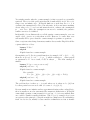
Another common use of Nitpick is to find out whether the axioms of a locale
are satisfiable, while the locale is being developed. To check this, it suffices
to write
lemma “False”
nitpick [show_all ]
after the locale’s begin keyword. To falsify False, Nitpick must find a model
for the axioms. If it finds no model, we have an indication that the axioms
might be unsatisfiable.
For Isabelle/jEdit users, Nitpick provides an automatic mode that can be
enabled via the “Auto Nitpick” option under “Plugins > Plugin Options >
Isabelle > General.” In this mode, Nitpick is run on every newly entered
theorem.
To run Nitpick, you must also make sure that the theory Nitpick is imported—
this is rarely a problem in practice since it is part of Main. The examples presented in this manual can be found in Isabelle’s src/HOL/Nitpick_
Examples/Manual_Nits.thy theory. The known bugs and limitations at the
time of writing are listed in §8. Comments and bug reports concerning either
the tool or the manual should be directed to the author at blannospam
chette@in.
tum.de.
Acknowledgment. The author would like to thank Mark Summerfield for
suggesting several textual improvements.
2
Installation
Nitpick is part of Isabelle, so you do not need to install it. It relies on a
third-party Kodkod front-end called Kodkodi, which in turn requires a Java
virtual machine. Both are provided as official Isabelle components.
To check whether Kodkodi is successfully installed, you can try out the example in §3.1.
3
3
First Steps
This section introduces Nitpick by presenting small examples. If possible, you
should try out the examples on your workstation. Your theory file should
start as follows:
theory Scratch
imports Main Quotient_Product RealDef
begin
The results presented here were obtained using the JNI (Java Native Interface) version of MiniSat and with multithreading disabled to reduce nondeterminism. This was done by adding the line
nitpick_params [sat_solver = MiniSat_JNI, max_threads = 1]
after the begin keyword. The JNI version of MiniSat is bundled with Kodkodi and is precompiled for Linux, Mac OS X, and Windows (Cygwin). Other
SAT solvers can also be used, as explained in §5.6. If you have already configured SAT solvers in Isabelle (e.g., for Refute), these will also be available
to Nitpick.
3.1
Propositional Logic
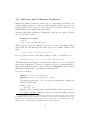
Let’s start with a trivial example from propositional logic:
lemma “P ←→ Q”
nitpick
You should get the following output:
Nitpick found a counterexample:
Free variables:
P = True
Q = False
Nitpick can also be invoked on individual subgoals, as in the example below:
apply auto
goal (2 subgoals):
1. P =⇒ Q
2. Q =⇒ P
4
nitpick 1
Nitpick found a counterexample:
Free variables:
P = True
Q = False
nitpick 2
Nitpick found a counterexample:
Free variables:
P = False
Q = True
oops
3.2
Type Variables
If you are left unimpressed by the previous example, don’t worry. The next
one is more mind- and computer-boggling:
lemma “x ∈ A =⇒ (THE y. y ∈ A) ∈ A”
The putative lemma involves the definite description operator, THE, presented in section 5.10.1 of the Isabelle tutorial [5]. The operator is defined
by the axiom (THE x . x = a) = a. The putative lemma is merely asserting
the indefinite description operator axiom with THE substituted for SOME.
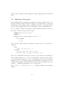
The free variable x and the bound variable y have type 0 a. For formulas
containing type variables, Nitpick enumerates the possible domains for each
type variable, up to a given cardinality (10 by default), looking for a finite
countermodel:
nitpick [verbose]
Trying 10 scopes:
card 0 a = 1;
card 0 a = 2;
..
.
card 0 a = 10.
Nitpick found a counterexample for card 0 a = 3:
5
Free variables:
A = {a2 , a3 }
x = a3
Total time: 963 ms.
Nitpick found a counterexample in which 0 a has cardinality 3. (For cardinalities 1 and 2, the formula holds.) In the counterexample, the three values of
type 0 a are written a1 , a2 , and a3 .
The message “Trying n scopes: . . . ” is shown only if the option verbose is
enabled. You can specify verbose each time you invoke nitpick, or you can
set it globally using the command
nitpick_params [verbose]
This command also displays the current default values for all of the options
supported by Nitpick. The options are listed in §5.
3.3
Constants
By just looking at Nitpick’s output, it might not be clear why the counterexample in §3.2 is genuine. Let’s invoke Nitpick again, this time telling it to
show the values of the constants that occur in the formula:
lemma “x ∈ A =⇒ (THE y. y ∈ A) ∈ A”
nitpick [show_consts]
Nitpick found a counterexample for card 0 a = 3:
Free variables:
A = {a2 , a3 }
x = a3
Constant:
THE y. y ∈ A = a1
As the result of an optimization, Nitpick directly assigned a value to the
subterm THE y. y ∈ A, rather than to the The constant. We can disable
this optimization by using the command
nitpick [dont_specialize, show_consts]
Our misadventures with THE suggest adding ‘∃!x .’ (“there exists a unique x
such that”) at the front of our putative lemma’s assumption:
6
lemma “∃!x . x ∈ A =⇒ (THE y. y ∈ A) ∈ A”
The fix appears to work:
nitpick
Nitpick found no counterexample.
We can further increase our confidence in the formula by exhausting all cardinalities up to 50:
nitpick [card 0 a = 1–50]1
Nitpick found no counterexample.
Let’s see if Sledgehammer can find a proof:
sledgehammer
Sledgehammer: “e” on goal
Try this: by (metis theI) (42 ms).
..
.
by (metis theI )
This must be our lucky day.
3.4
Skolemization
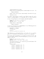
Are all invertible functions onto? Let’s find out:
lemma “∃g. ∀x . g (f x ) = x =⇒ ∀y. ∃x . y = f x ”
nitpick
Nitpick found a counterexample for card 0 a = 2 and card 0 b = 1:
Free variable:
f = (λx . _)(b1 := a1 )
Skolem constants:
g = (λx . _)(a1 := b1 , a2 := b1 )
y = a2
(The Isabelle/HOL notation f (x := y) denotes the function that maps x to
y and that otherwise behaves like f .) Although f is the only free variable
1
The symbol ‘–’ can be entered as - (hyphen) or \<emdash>.
7
occurring in the formula, Nitpick also displays values for the bound variables g and y. These values are available to Nitpick because it performs
skolemization as a preprocessing step.
In the previous example, skolemization only affected the outermost quantifiers. This is not always the case, as illustrated below:
lemma “∃x . ∀f . f x = x ”
nitpick
Nitpick found a counterexample for card 0 a = 2:
Skolem constant:
λx . f = (λx . _)(a1 := (λx . _)(a1 := a2 , a2 := a1 ),
a2 := (λx . _)(a1 := a1 , a2 := a1 ))
The variable f is bound within the scope of x ; therefore, f depends on x , as
suggested by the notation λx . f . If x = a1 , then f is the function that maps
a1 to a2 and vice versa; otherwise, x = a2 and f maps both a1 and a2 to a1 .
In both cases, f x 6= x .
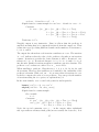
The source of the Skolem constants is sometimes more obscure:
lemma “refl r =⇒ sym r ”
nitpick
Nitpick found a counterexample for card 0 a = 2:
Free variable:
r = {(a1 , a1 ), (a2 , a1 ), (a2 , a2 )}
Skolem constants:
sym.x = a2
sym.y = a1
What happened here is that Nitpick expanded sym to its definition:
sym r ≡ ∀x y. (x , y) ∈ r −→ (y, x ) ∈ r .
As their names suggest, the Skolem constants sym.x and sym.y are simply
the bound variables x and y from sym’s definition.
3.5
Natural Numbers and Integers
Because of the axiom of infinity, the type nat does not admit any finite
models. To deal with this, Nitpick’s approach is to consider finite subsets
8
N of nat and maps all numbers ∈
/ N to the undefined value (displayed as
‘_’). The type int is handled similarly. Internally, undefined values lead to
a three-valued logic.
Here is an example involving int:
lemma “[[i ≤ j ; n ≤ (m::int)]] =⇒ i ∗ n + j ∗ m ≤ i ∗ m + j ∗ n”
nitpick
Nitpick found a counterexample:
Free variables:
i =0
j =1
m=1
n=0
Internally, Nitpick uses either a unary or a binary representation of numbers.
The unary representation is more efficient but only suitable for numbers very
close to zero. By default, Nitpick attempts to choose the more appropriate
encoding by inspecting the formula at hand. This behavior can be overridden
by passing either unary_ints or binary_ints as option. For binary notation,
the number of bits to use can be specified using the bits option. For example:
nitpick [binary_ints, bits = 16]
With infinite types, we don’t always have the luxury of a genuine counterexample and must often content ourselves with a potentially spurious one.
The tedious task of finding out whether the potentially spurious counterexample is in fact genuine can be delegated to auto by passing check_potential.
For example:
lemma “∀n. Suc n 6= n =⇒ P ”
nitpick [card nat = 50, check_potential ]
Warning: The conjecture either trivially holds for the given scopes or
lies outside Nitpick’s supported fragment. Only potentially spurious
counterexamples may be found.
Nitpick found a potentially spurious counterexample:
Free variable:
P = False
Confirmation by “auto”: The above counterexample is genuine.
9
You might wonder why the counterexample is first reported as potentially
spurious. The root of the problem is that the bound variable in ∀n. Suc n 6= n
ranges over an infinite type. If Nitpick finds an n such that Suc n = n, it
evaluates the assumption to False; but otherwise, it does not know anything
about values of n ≥ card nat and must therefore evaluate the assumption
to _, not True. Since the assumption can never be satisfied, the putative
lemma can never be falsified.
Incidentally, if you distrust the so-called genuine counterexamples, you can
enable check_genuine to verify them as well. However, be aware that auto
will usually fail to prove that the counterexample is genuine or spurious.
Some conjectures involving elementary number theory make Nitpick look like
a giant with feet of clay:
lemma “P Suc”
nitpick
Nitpick found no counterexample.
On any finite set N , Suc is a partial function; for example, if N = {0, 1, . . . , k },
then Suc is {0 7→ 1, 1 7→ 2, . . . , k 7→ _}, which evaluates to _ when passed
as argument to P . As a result, P Suc is always _. The next example is
similar:
lemma “P (op +::nat ⇒ nat ⇒ nat)”
nitpick [card nat = 1]
Nitpick found a counterexample:
Free variable:
P = (λx . _)((λx . _)(0 := (λx . _)(0 := 0)) := False)
nitpick [card nat = 2]
Nitpick found no counterexample.
The problem here is that op + is total when nat is taken to be {0} but
becomes partial as soon as we add 1, because 1 + 1 ∈
/ {0, 1}.
Because numbers are infinite and are approximated using a three-valued logic,
there is usually no need to systematically enumerate domain sizes. If Nitpick
cannot find a genuine counterexample for card nat = k , it is very unlikely that
one could be found for smaller domains. (The P (op +) example above is an
exception to this principle.) Nitpick nonetheless enumerates all cardinalities
from 1 to 10 for nat, mainly because smaller cardinalities are fast to handle
10
and give rise to simpler counterexamples. This is explained in more detail in
§3.11.
3.6
Inductive Datatypes
Like natural numbers and integers, inductive datatypes with recursive constructors admit no finite models and must be approximated by a subtermclosed subset. For example, using a cardinality of 10 for 0 a list, Nitpick looks
for all counterexamples that can be built using at most 10 different lists.
Let’s see with an example involving hd (which returns the first element of a
list) and @ (which concatenates two lists):
lemma “hd (xs @ [y, y]) = hd xs”
nitpick
Nitpick found a counterexample for card 0 a = 3:
Free variables:
xs = []
y = a1
To see why the counterexample is genuine, we enable show_consts and show_
datatypes:
Type:
0
a list = {[], [a1 ], [a1 , a1 ], . . .}
Constants:
λx1 . x1 @ [y, y] = (λx . _)([] := [a1 , a1 ])
hd = (λx . _)([] := a2 , [a1 ] := a1 , [a1 , a1 ] := a1 )
Since hd [] is undefined in the logic, it may be given any value, including a2 .
The second constant, λx1 . x1 @ [y, y], is simply the append operator whose
second argument is fixed to be [y, y]. Appending [a1 , a1 ] to [a1 ] would normally give [a1 , a1 , a1 ], but this value is not representable in the subset of 0 a list
considered by Nitpick, which is shown under the “Type” heading; hence the
result is _. Similarly, appending [a1 , a1 ] to itself gives _.
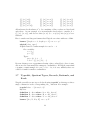
Given card 0 a = 3 and card 0 a list = 3, Nitpick considers the following
subsets:
11
{[],
{[],
{[],
{[],
[a1 ],
[a1 ],
[a2 ],
[a1 ],
[a2 ]};
[a3 ]};
[a3 ]};
[a1 , a1 ]};
{[],
{[],
{[],
{[],
[a1 ],
[a1 ],
[a2 ],
[a2 ],
[a2 , a1 ]};
[a3 , a1 ]};
[a1 , a2 ]};
[a2 , a2 ]};
{[],
{[],
{[],
{[],
[a2 ],
[a3 ],
[a3 ],
[a3 ],
[a3 , a2 ]};
[a1 , a3 ]};
[a2 , a3 ]};
[a3 , a3 ]}.
All subterm-closed subsets of 0 a list consisting of three values are listed and
only those. As an example of a non-subterm-closed subset, consider S =
{[], [a1 ], [a1 , a2 ]}, and observe that [a1 , a2 ] (i.e., a1 # [a2 ]) has [a2 ] ∈
/ S as a
subterm.
Here’s another möchtegern-lemma that Nitpick can refute without a blink:
lemma “[[length xs = 1; length ys = 1]] =⇒ xs = ys”
nitpick [show_types]
Nitpick found a counterexample for card 0 a = 3:
Free variables:
xs = [a2 ]
ys = [a1 ]
Types:
nat = {0, 1, 2, . . .}
0
a list = {[], [a1 ], [a2 ], . . .}
Because datatypes are approximated using a three-valued logic, there is usually no need to systematically enumerate cardinalities: If Nitpick cannot find
a genuine counterexample for card 0 a list = 10, it is very unlikely that one
could be found for smaller cardinalities.
3.7
Typedefs, Quotient Types, Records, Rationals, and
Reals
Nitpick generally treats types declared using typedef as datatypes whose
single constructor is the corresponding Abs_ function. For example:
typedef three = “{0::nat, 1, 2}”
by blast
definition A :: three where “A ≡ Abs_three 0”
definition B :: three where “B ≡ Abs_three 1”
definition C :: three where “C ≡ Abs_three 2”
lemma “[[A ∈ X ; B ∈ X ]] =⇒ c ∈ X ”
12
nitpick [show_types]
Nitpick found a counterexample:
Free variables:
X = {« 0 », « 1 »}
c = «2»
Types:
nat = {0, 1, 2, . . .}
three = {« 0 », « 1 », « 2 », . . .}
In the output above, « n » abbreviates Abs_three n.
Quotient types are handled in much the same way. The following fragment
defines the integer type my_int by encoding the integer x by a pair of natural
numbers (m, n) such that x + n = m:
fun my_int_rel where
“my_int_rel (x , y) (u, v ) = (x + v = u + y)”
quotient_type my_int = “nat × nat” / my_int_rel
by (auto simp add : equivp_def fun_eq_iff )
definition add_raw where
“add_raw ≡ λ(x , y) (u, v ). (x + (u::nat), y + (v ::nat))”
quotient_definition “add ::my_int ⇒ my_int ⇒ my_int” is add_raw
lemma “add x y = add x x ”
nitpick [show_types]
Nitpick found a counterexample:
Free variables:
x = « (0, 0) »
y = « (0, 1) »
Types:
nat = {0, 1, . . .}
nat × nat [boxed] = {(0, 0), (1, 0), . . .}
my_int = {« (0, 0) », « (0, 1) », . . .}
The values « (0, 0) » and « (0, 1) » represent the integers 0 and −1, respectively. Other representants would have been possible—e.g., « (5, 5) » and
« (11, 12) ». If we are going to use my_int extensively, it pays off to install a term postprocessor that converts the pair notation to the standard
mathematical notation:
13
ML {∗
fun my_int_postproc _ _ _ T (Const _ $ (Const _ $ t1 $ t2 )) =
HOLogic.mk_number T (snd (HOLogic.dest_number t1)
− snd (HOLogic.dest_number t2 ))
| my_int_postproc _ _ _ _ t = t
∗}
declaration {∗
Nitpick_Model.register_term_postprocessor @{typ my_int}
my_int_postproc
∗}
Records are handled as datatypes with a single constructor:
record point =
Xcoord :: int
Ycoord :: int
lemma “Xcoord (p::point) = Xcoord (q::point)”
nitpick [show_types]
Nitpick found a counterexample:
Free variables:
p = (|Xcoord = 1, Ycoord = 1|)
q = (|Xcoord = 0, Ycoord = 0|)
Types:
int = {0, 1, . . .}
point = {(|Xcoord = 0, Ycoord = 0|),
(|Xcoord = 1, Ycoord = 1|), . . .}
Finally, Nitpick provides rudimentary support for rationals and reals using a
similar approach:
lemma “4 ∗ x + 3 ∗ (y::real) 6= 1/2”
nitpick [show_types]
Nitpick found a counterexample:
Free variables:
x = 1/2
y = −1/2
Types:
nat = {0, 1, 2, 3, 4, 5, 6, 7, . . .}
int = {−3, −2, −1, 0, 1, 2, 3, 4, . . .}
real = {−3/2, −1/2, 0, 1/2, 1, 2, 3, 4, . . .}
14
3.8
Inductive and Coinductive Predicates
Inductively defined predicates (and sets) are particularly problematic for
counterexample generators. They can make Quickcheck [2] loop forever and
Refute [8] run out of resources. The crux of the problem is that they are
defined using a least fixed-point construction.
Nitpick’s philosophy is that not all inductive predicates are equal. Consider
the even predicate below:
inductive even where
“even 0” |
“even n =⇒ even (Suc (Suc n))”
This predicate enjoys the desirable property of being well-founded, which
means that the introduction rules don’t give rise to infinite chains of the
form
· · · =⇒ even k 00 =⇒ even k 0 =⇒ even k .
For even, this is obvious: Any chain ending at k will be of length k /2 + 1:
even 0 =⇒ even 2 =⇒ · · · =⇒ even (k − 2) =⇒ even k .
Wellfoundedness is desirable because it enables Nitpick to use a very efficient
fixed-point computation.2 Moreover, Nitpick can prove wellfoundedness of
most well-founded predicates, just as Isabelle’s function package usually
discharges termination proof obligations automatically.
Let’s try an example:
lemma “∃n. even n ∧ even (Suc n)”
nitpick [card nat = 50, unary_ints, verbose]
The inductive predicate “even” was proved well-founded. Nitpick can
compute it efficiently.
Trying 1 scope:
card nat = 50.
Warning: The conjecture either trivially holds for the given scopes or
lies outside Nitpick’s supported fragment. Only potentially spurious
2
If an inductive predicate is well-founded, then it has exactly one fixed point, which
is simultaneously the least and the greatest fixed point. In these circumstances, the computation of the least fixed point amounts to the computation of an arbitrary fixed point,
which can be performed using a straightforward recursive equation.
15
counterexamples may be found.
Nitpick found a potentially spurious counterexample for card nat = 50:
Empty assignment
Nitpick could not find a better counterexample. It checked 1 of 1 scope.
Total time: 1.62 s.
No genuine counterexample is possible because Nitpick cannot rule out the
existence of a natural number n ≥ 50 such that both even n and even (Suc n)
are true. To help Nitpick, we can bound the existential quantifier:
lemma “∃n ≤ 49. even n ∧ even (Suc n)”
nitpick [card nat = 50, unary_ints]
Nitpick found a counterexample:
Empty assignment
So far we were blessed by the wellfoundedness of even. What happens if we
use the following definition instead?
inductive even0 where
“even0 (0::nat)” |
“even0 2” |
“[[even0 m; even0 n]] =⇒ even0 (m + n)”
This definition is not well-founded: From even0 0 and even0 0, we can derive
that even0 0. Nonetheless, the predicates even and even0 are equivalent.
Let’s check a property involving even0 . To make up for the foreseeable computational hurdles entailed by non-wellfoundedness, we decrease nat’s cardinality to a mere 10:
lemma “∃n ∈ {0, 2, 4, 6, 8}. ¬ even0 n”
nitpick [card nat = 10, verbose, show_consts]
The inductive predicate “even0” could not be proved well-founded. Nitpick might need to unroll it.
Trying 6 scopes:
card nat = 10
card nat = 10
card nat = 10
card nat = 10
card nat = 10
and
and
and
and
and
iter
iter
iter
iter
iter
even0
even0
even0
even0
even0
16
=
=
=
=
=
0;
1;
2;
4;
8;
card nat = 10 and iter even0 = 9.
Nitpick found a counterexample for card nat = 10 and iter even0 = 2:
Constant:
λi . even0 = (λx . _)(0 := (λx . _)(0 := True,
1 := (λx . _)(0 := True,
2 := (λx . _)(0 := True,
6 := True,
2 := True),
2 := True, 4 := True),
2 := True, 4 := True,
8 := True))
Total time: 1.87 s.
Nitpick’s output is very instructive. First, it tells us that the predicate is
unrolled, meaning that it is computed iteratively from the empty set. Then
it lists six scopes specifying different bounds on the numbers of iterations: 0,
1, 2, 4, 8, and 9.
The output also shows how each iteration contributes to even0 . The notation
λi . even0 indicates that the value of the predicate depends on an iteration
counter. Iteration 0 provides the basis elements, 0 and 2. Iteration 1 contributes 4 (= 2 + 2). Iteration 2 throws 6 (= 2 + 4 = 4 + 2) and 8 (= 4 + 4)
into the mix. Further iterations would not contribute any new elements. The
predicate even0 evaluates to either True or _, never False.
When unrolling a predicate, Nitpick tries 0, 1, 2, 4, 8, 12, 16, 20, 24, and
28 iterations. However, these numbers are bounded by the cardinality of the
predicate’s domain. With card nat = 10, no more than 9 iterations are ever
needed to compute the value of a nat predicate. You can specify the number
of iterations using the iter option, as explained in §5.2.
In the next formula, even0 occurs both positively and negatively:
lemma “even0 (n − 2) =⇒ even0 n”
nitpick [card nat = 10, show_consts]
Nitpick found a counterexample:
Free variable:
n=1
Constants:
λi . even0 = (λx . _)(0 := (λx . _)(0 := True, 2 := True))
even0 ≤ (λx . _)(0 := True, 1 := False, 2 := True,
4 := True, 6 := True, 8 := True)
Notice the special constraint even0 ≤ . . . in the output, whose right-hand
side represents an arbitrary fixed point (not necessarily the least one). It is
17
used to falsify even0 n. In contrast, the unrolled predicate is used to satisfy
even0 (n − 2).
Coinductive predicates are handled dually. For example:
coinductive nats where
“nats (x ::nat) =⇒ nats x ”
lemma “nats = (λn. n ∈ {0, 1, 2, 3, 4})”
nitpick [card nat = 10, show_consts]
Nitpick found a counterexample:
Constants:
λi . nats = (λx . _)(0 := (λx . _), 1 := (λx . _), 2 := (λx . _))
nats ≥ (λx . _)(3 := True, 4 := False, 5 := True)
As a special case, Nitpick uses Kodkod’s transitive closure operator to encode negative occurrences of non-well-founded “linear inductive predicates,”
i.e., inductive predicates for which each the predicate occurs in at most one
assumption of each introduction rule. For example:
inductive odd where
“odd 1” |
“[[odd m; even n]] =⇒ odd (m + n)”
lemma “odd n =⇒ odd (n − 2)”
nitpick [card nat = 4, show_consts]
Nitpick found a counterexample:
Free variable:
n=1
Constants:
even = (λx . _)(0 := True, 1 := False, 2 := True, 3 := False)
oddbase =
(λx . _)(0 := False, 1 := True, 2 := False, 3 := False)
oddstep = (λx . _)
(0 := (λx . _)(0 := True, 1 := False, 2 := True, 3 := False),
1 := (λx . _)(0 := False, 1 := True, 2 := False, 3 := True),
2 := (λx . _)(0 := False, 1 := False, 2 := True, 3 := False),
3 := (λx . _)(0 := False, 1 := False, 2 := False, 3 := True))
odd ≤ (λx . _)(0 := False, 1 := True, 2 := False, 3 := True)
In the output, oddbase represents the base elements and oddstep is a transition
relation that computes new elements from known ones. The set odd consists
18
of all the values reachable through the reflexive transitive closure of oddstep
starting with any element from oddbase , namely 1 and 3. Using Kodkod’s
transitive closure to encode linear predicates is normally either more thorough
or more efficient than unrolling (depending on the value of iter ), but you can
disable it by passing the dont_star_linear_preds option.
3.9
Coinductive Datatypes
A coinductive datatype is similar to an inductive datatype but allows infinite
objects. Thus, the infinite lists ps = [a, a, a, . . .], qs = [a, b, a, b, . . .], and rs
= [0, 1, 2, 3, . . .] can be defined as coinductive lists, or “lazy lists,” using the
LNil :: 0 a llist and LCons :: 0 a ⇒ 0 a llist ⇒ 0 a llist constructors.
Although it is otherwise no friend of infinity, Nitpick can find counterexamples involving cyclic lists such as ps and qs above as well as finite lists:
codatatype 0 a llist = LNil | LCons 0 a “ 0 a llist”
lemma “xs 6= LCons a xs”
nitpick
Nitpick found a counterexample for card 0 a = 1:
Free variables:
a = a1
xs = THE ω. ω = LCons a1 ω
The notation THE ω. ω = t(ω) stands for the infinite term t(t(t(. . .))).
Hence, xs is simply the infinite list [a1 , a1 , a1 , . . .].
The next example is more interesting:
primcorec iterates where
“iterates f a = LCons a (iterates f (f a))”
lemma “[[xs = LCons a xs; ys = iterates (λb. a) b]] =⇒ xs = ys”
nitpick [verbose]
The type 0 a passed the monotonicity test. Nitpick might be able to
skip some scopes.
Trying 10 scopes:
card 0 a = 1, card “ 0 a list” = 1, and bisim_depth = 0.
..
.
card 0 a = 10, card “ 0 a list” = 10, and bisim_depth = 9.
19
Nitpick found a counterexample for card 0 a = 2, card “ 0 a llist” = 2, and
bisim_depth = 1:
Free variables:
a = a1
b = a2
xs = THE ω. ω = LCons a1 ω
ys = LCons a2 (THE ω. ω = LCons a1 ω)
Total time: 1.11 s.
The lazy list xs is simply [a1 , a1 , a1 , . . .], whereas ys is [a2 , a1 , a1 , a1 , . . .], i.e.,
a lasso-shaped list with [a2 ] as its stem and [a1 ] as its cycle. In general, the
list segment within the scope of the THE binder corresponds to the lasso’s
cycle, whereas the segment leading to the binder is the stem.
A salient property of coinductive datatypes is that two objects are considered
equal if and only if they lead to the same observations. For example, the two
lazy lists
THE ω. ω = LCons a (LCons b ω)
LCons a (THE ω. ω = LCons b (LCons a ω))
are identical, because both lead to the sequence of observations a, b, a, b, . . .
(or, equivalently, both encode the infinite list [a, b, a, b, . . .]). This concept
of equality for coinductive datatypes is called bisimulation and is defined
coinductively.
Internally, Nitpick encodes the coinductive bisimilarity predicate as part of
the Kodkod problem to ensure that distinct objects lead to different observations. This precaution is somewhat expensive and often unnecessary, so it
can be disabled by setting the bisim_depth option to −1. The bisimilarity
check is then performed after the counterexample has been found to ensure
correctness. If this after-the-fact check fails, the counterexample is tagged as
“quasi genuine” and Nitpick recommends to try again with bisim_depth set
to a nonnegative integer.
The next formula illustrates the need for bisimilarity (either as a Kodkod
predicate or as an after-the-fact check) to prevent spurious counterexamples:
lemma “[[xs = LCons a xs; ys = LCons a ys]] =⇒ xs = ys”
nitpick [bisim_depth = −1, show_types]
Nitpick found a quasi genuine counterexample for card 0 a = 2:
20
Free variables:
a = a1
xs = THE ω. ω = LCons a1 ω
ys = THE ω. ω = LCons a1 ω
Type:
0
a llist = {THE ω. ω = LCons a1 ω,
THE ω. ω = LCons a1 ω, . . .}
Try again with “bisim_depth” set to a nonnegative value to confirm
that the counterexample is genuine.
nitpick
Nitpick found no counterexample.
In the first nitpick invocation, the after-the-fact check discovered that the
two known elements of type 0 a llist are bisimilar, prompting Nitpick to label
the example as only “quasi genuine.”
A compromise between leaving out the bisimilarity predicate from the Kodkod problem and performing the after-the-fact check is to specify a low nonnegative bisim_depth value. In general, a value of K means that Nitpick
will require all lists to be distinguished from each other by their prefixes of
length K . However, setting K to a too low value can overconstrain Nitpick,
preventing it from finding any counterexamples.
3.10
Boxing
Nitpick normally maps function and product types directly to the corresponding Kodkod concepts. As a consequence, if 0 a has cardinality 3 and 0 b
has cardinality 4, then 0 a × 0 b has cardinality 12 (= 4 × 3) and 0 a ⇒ 0 b has
cardinality 64 (= 43 ). In some circumstances, it pays off to treat these types
in the same way as plain datatypes, by approximating them by a subset of a
given cardinality. This technique is called “boxing” and is particularly useful
for functions passed as arguments to other functions, for high-arity functions,
and for large tuples. Under the hood, boxing involves wrapping occurrences
of the types 0 a × 0 b and 0 a ⇒ 0 b in isomorphic datatypes, as can be seen by
enabling the debug option.
To illustrate boxing, we consider a formalization of λ-terms represented using
de Bruijn’s notation:
datatype tm = Var nat | Lam tm | App tm tm
21
The lift t k function increments all variables with indices greater than or
equal to k by one:
primrec lift where
“lift (Var j ) k = Var (if j < k then j else j + 1)” |
“lift (Lam t) k = Lam (lift t (k + 1))” |
“lift (App t u) k = App (lift t k ) (lift u k )”
The loose t k predicate returns True if and only if term t has a loose variable
with index k or more:
primrec loose where
“loose (Var j ) k = (j ≥ k )” |
“loose (Lam t) k = loose t (Suc k )” |
“loose (App t u) k = (loose t k ∨ loose u k )”
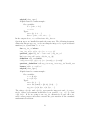
Next, the subst σ t function applies the substitution σ on t:
primrec subst where
“subst σ (Var j ) = σ j ” |
“subst σ (Lam t) =
Lam (subst (λn. case n of 0 ⇒ Var 0 | Suc m ⇒ lift (σ m) 1) t)” |
“subst σ (App t u) = App (subst σ t) (subst σ u)”
A substitution is a function that maps variable indices to terms. Observe
that σ is a function passed as argument and that Nitpick can’t optimize it
away, because the recursive call for the Lam case involves an altered version.
Also notice the lift call, which increments the variable indices when moving
under a Lam.
A reasonable property to expect of substitution is that it should leave closed
terms unchanged. Alas, even this simple property does not hold:
lemma “¬ loose t 0 =⇒ subst σ t = t”
nitpick [verbose]
Trying 10 scopes:
card nat = 1, card tm = 1, and card “nat ⇒ tm” = 1;
card nat = 2, card tm = 2, and card “nat ⇒ tm” = 2;
..
.
card nat = 10, card tm = 10, and card “nat ⇒ tm” = 10.
Nitpick found a counterexample for card nat = 6, card tm = 6,
and card “nat ⇒ tm” = 6:
22
Free variables:
σ = (λx . _)(0 := Var 0, 1 := Var 0, 2 := Var 0,
3 := Var 0, 4 := Var 0, 5 := Lam (Lam (Var 0)))
t = Lam (Lam (Var 1))
Total time: 3.08 s.
Using eval, we find out that subst σ t = Lam (Lam (Var 0)). Using the
traditional λ-calculus notation, t is λx y. x whereas subst σ t is (wrongly)
λx y. y. The bug is in subst: The lift (σ m) 1 call should be replaced with
lift (σ m) 0.
An interesting aspect of Nitpick’s verbose output is that it assigned inceasing
cardinalities from 1 to 10 to the type nat ⇒ tm of the higher-order argument
σ of subst. For the formula of interest, knowing 6 values of that type was
enough to find the counterexample. Without boxing, 66 = 46 656 values must
be considered, a hopeless undertaking:
nitpick [dont_box ]
Nitpick ran out of time after checking 3 of 10 scopes.
Boxing can be enabled or disabled globally or on a per-type basis using the
box option. Nitpick usually performs reasonable choices about which types
should be boxed, but option tweaking sometimes helps.
3.11
Scope Monotonicity
The card option (together with iter, bisim_depth, and max ) controls which
scopes are actually tested. In general, to exhaust all models below a certain
cardinality bound, the number of scopes that Nitpick must consider increases
exponentially with the number of type variables (and typedecl’d types)
occurring in the formula. Given the default cardinality specification of 1–10,
no fewer than 104 = 10 000 scopes must be considered for a formula involving
0
a, 0 b, 0 c, and 0 d .
Fortunately, many formulas exhibit a property called scope monotonicity,
meaning that if the formula is falsifiable for a given scope, it is also falsifiable
for all larger scopes [4, p. 165].
Consider the formula
lemma “length xs = length ys =⇒ rev (zip xs ys) = zip xs (rev ys)”
23
where xs is of type 0 a list and ys is of type 0 b list. A priori, Nitpick would
need to consider 1 000 scopes to exhaust the specification card = 1–10 (10
cardinalies for 0 a × 10 cardinalities for 0 b × 10 cardinalities for the datatypes).
However, our intuition tells us that any counterexample found with a small
scope would still be a counterexample in a larger scope—by simply ignoring
the fresh 0 a and 0 b values provided by the larger scope. Nitpick comes to the
same conclusion after a careful inspection of the formula and the relevant
definitions:
nitpick [verbose]
The types 0 a and 0 b passed the monotonicity test. Nitpick might be
able to skip some scopes.
Trying 10 scopes:
card 0 a = 1, card 0 b = 1, card nat
card “ 0 a list” = 1, and card “ 0 b
card 0 a = 2, card 0 b = 2, card nat
card “ 0 a list” = 2, and card “ 0 b
..
.
= 1, card “(0 a × 0 b) list” = 1,
list” = 1.
= 2, card “(0 a × 0 b) list” = 2,
list” = 2.
card 0 a = 10, card 0 b = 10, card nat = 10, card “(0 a × 0 b) list” =
10,
card “ 0 a list” = 10, and card “ 0 b list” = 10.
Nitpick found a counterexample for card 0 a = 5, card 0 b = 5, card nat =
5, card “(0 a × 0 b) list” = 5, card “ 0 a list” = 5, and card “ 0 b list” = 5:
Free variables:
xs = [a1 , a2 ]
ys = [b1 , b1 ]
Total time: 1.63 s.
In theory, it should be sufficient to test a single scope:
nitpick [card = 10]
However, this is often less efficient in practice and may lead to overly complex
counterexamples.
If the monotonicity check fails but we believe that the formula is monotonic
(or we don’t mind missing some counterexamples), we can pass the mono
option. To convince yourself that this option is risky, simply consider this
example from §3.4:
24
lemma “∃g. ∀x ::0 b. g (f x ) = x =⇒ ∀y::0 a. ∃x . y = f x ”
nitpick [mono]
Nitpick found no counterexample.
nitpick
Nitpick found a counterexample for card 0 a = 2 and card 0 b = 1:
..
.
(It turns out the formula holds if and only if card 0 a ≤ card 0 b.) Although
this is rarely advisable, the automatic monotonicity checks can be disabled
by passing non_mono (§5.6).
As insinuated in §3.5 and §3.6, nat, int, and inductive datatypes are normally
monotonic and treated as such. The same is true for record types, rat, and
real. Thus, given the cardinality specification 1–10, a formula involving nat,
int, int list, rat, and rat list will lead Nitpick to consider only 10 scopes
instead of 104 = 10 000. On the other hand, typedef s and quotient types
are generally nonmonotonic.
3.12
Inductive Properties
Inductive properties are a particular pain to prove, because the failure to
establish an induction step can mean several things:
1. The property is invalid.
2. The property is valid but is too weak to support the induction step.
3. The property is valid and strong enough; it’s just that we haven’t found
the proof yet.
Depending on which scenario applies, we would take the appropriate course
of action:
1. Repair the statement of the property so that it becomes valid.
2. Generalize the property and/or prove auxiliary properties.
3. Work harder on a proof.
25
How can we distinguish between the three scenarios? Nitpick’s normal mode
of operation can often detect scenario 1, and Isabelle’s automatic tactics help
with scenario 3. Using appropriate techniques, it is also often possible to use
Nitpick to identify scenario 2. Consider the following transition system, in
which natural numbers represent states:
inductive_set reach where
“(4::nat) ∈ reach” |
“[[n < 4; n ∈ reach]] =⇒ 3 ∗ n + 1 ∈ reach” |
“n ∈ reach =⇒ n + 2 ∈ reach”
We will try to prove that only even numbers are reachable:
lemma “n ∈ reach =⇒ 2 dvd n”
Does this property hold? Nitpick cannot find a counterexample within 30
seconds, so let’s attempt a proof by induction:
apply (induct set: reach)
apply auto
This leaves us in the following proof state:
goalV(2 subgoals):
1. Vn. [[n ∈ reach; n < 4; 2 dvd n]] =⇒ 2 dvd Suc (3 ∗ n)
2. n. [[n ∈ reach; 2 dvd n]] =⇒ 2 dvd Suc (Suc n)
If we run Nitpick on the first subgoal, it still won’t find any counterexample;
and yet, auto fails to go further, and arith is helpless. However, notice the
n ∈ reach assumption, which strengthens the induction hypothesis but is not
immediately usable in the proof. If we remove it and invoke Nitpick, this
time we get a counterexample:
apply (thin_tac “n ∈ reach”)
nitpick
Nitpick found a counterexample:
Skolem constant:
n=0
Indeed, 0 < 4, 2 divides 0, but 2 does not divide 1. We can use this information to strength the lemma:
lemma “n ∈ reach =⇒ 2 dvd n ∨ n 6= 0”
26
Unfortunately, the proof by induction still gets stuck, except that Nitpick
now finds the counterexample n = 2. We generalize the lemma further to
lemma “n ∈ reach =⇒ 2 dvd n ∨ n ≥ 4”
and this time arith can finish off the subgoals.
4
Case Studies
As a didactic device, the previous section focused mostly on toy formulas
whose validity can easily be assessed just by looking at the formula. We
will now review two somewhat more realistic case studies that are within
Nitpick’s reach: a context-free grammar modeled by mutually inductive sets
and a functional implementation of AA trees. The results presented in this
section were produced with the following settings:
nitpick_params [max_potential = 0]
4.1
A Context-Free Grammar
Our first case study is taken from section 7.4 in the Isabelle tutorial [5].
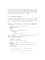
The following grammar, originally due to Hopcroft and Ullman, produces all
strings with an equal number of a’s and b’s:
S ::= | bA | aB
A ::= aS | bAA
B ::= bS | aBB
The intuition behind the grammar is that A generates all strings with one
more a than b’s and B generates all strings with one more b than a’s.
The alphabet consists exclusively of a’s and b’s:
datatype alphabet = a | b
Strings over the alphabet are represented by alphabet lists. Nonterminals in
the grammar become sets of strings. The production rules presented above
can be expressed as a mutually inductive definition:
inductive_set S and A and B where
R1 : “[] ∈ S ” |
R2 : “w ∈ A =⇒ b # w ∈ S ” |
27
R3 :
R4 :
R5 :
R6 :
“w ∈ B =⇒ a # w ∈ S ” |
“w ∈ S =⇒ a # w ∈ A” |
“w ∈ S =⇒ b # w ∈ S ” |
“[[v ∈ B ; v ∈ B ]] =⇒ a # v @ w ∈ B ”
The conversion of the grammar into the inductive definition was done manually by Joe Blow, an underpaid undergraduate student. As a result, some
errors might have sneaked in.
Debugging faulty specifications is at the heart of Nitpick’s raison d’être. A
good approach is to state desirable properties of the specification (here, that
S is exactly the set of strings over {a, b} with as many a’s as b’s) and check
them with Nitpick. If the properties are correctly stated, counterexamples
will point to bugs in the specification. For our grammar example, we will
proceed in two steps, separating the soundness and the completeness of the
set S . First, soundness:
theorem S_sound :
“w ∈ S −→ length [x ← w . x = a] = length [x ← w . x = b]”
nitpick
Nitpick found a counterexample:
Free variable:
w = [b]
It would seem that [b] ∈ S . How could this be? An inspection of the
introduction rules reveals that the only rule with a right-hand side of the
form b # . . . ∈ S that could have introduced [b] into S is R5 :
“w ∈ S =⇒ b # w ∈ S ”
On closer inspection, we can see that this rule is wrong. To match the
production B ::= bS , the second S should be a B . We fix the typo and try
again:
nitpick
Nitpick found a counterexample:
Free variable:
w = [a, a, b]
Some detective work is necessary to find out what went wrong here. To get
[a, a, b] ∈ S , we need [a, b] ∈ B by R3, which in turn can only come from
R6 :
28
“[[v ∈ B ; v ∈ B ]] =⇒ a # v @ w ∈ B ”
Now, this formula must be wrong: The same assumption occurs twice, and
the variable w is unconstrained. Clearly, one of the two occurrences of v in
the assumptions should have been a w .
With the correction made, we don’t get any counterexample from Nitpick.
Let’s move on and check completeness:
theorem S_complete:
“length [x ← w . x = a] = length [x ← w . x = b] −→ w ∈ S ”
nitpick
Nitpick found a counterexample:
Free variable:
w = [b, b, a, a]
Apparently, [b, b, a, a] ∈
/ S , even though it has the same numbers of a’s
and b’s. But since our inductive definition passed the soundness check, the
introduction rules we have are probably correct. Perhaps we simply lack an
introduction rule. Comparing the grammar with the inductive definition, our
suspicion is confirmed: Joe Blow simply forgot the production A ::= bAA,
without which the grammar cannot generate two or more b’s in a row. So
we add the rule
“[[v ∈ A; w ∈ A]] =⇒ b # v @ w ∈ A”
With this last change, we don’t get any counterexamples from Nitpick for
either soundness or completeness. We can even generalize our result to cover
A and B as well:
theorem S_A_B_sound_and_complete:
“w ∈ S ←→ length [x ← w . x = a] = length [x ← w . x = b]”
“w ∈ A ←→ length [x ← w . x = a] = length [x ← w . x = b] + 1”
“w ∈ B ←→ length [x ← w . x = b] = length [x ← w . x = a] + 1”
nitpick
Nitpick found no counterexample.
4.2
AA Trees
AA trees are a kind of balanced trees discovered by Arne Andersson that
provide similar performance to red-black trees, but with a simpler implementation [1]. They can be used to store sets of elements equipped with a
29
total order <. We start by defining the datatype and some basic extractor
functions:
datatype 0 a aa_tree =
Λ | N “ 0 a::linorder ” nat “ 0 a aa_tree” “ 0 a aa_tree”
primrec data where
“data Λ = (λx . _)” |
“data (N x _ _ _) = x ”
primrec dataset where
“dataset Λ = {}” |
“dataset (N x _ t u) = {x } ∪ dataset t ∪ dataset u”
primrec level where
“level Λ = 0” |
“level (N _ k _ _) = k ”
primrec left where
“left Λ = Λ” |
“left (N _ _ t _) = t”
primrec right where
“right Λ = Λ” |
“right (N _ _ _ u) = u”
The wellformedness criterion for AA trees is fairly complex. Wikipedia states
it as follows [9]:
Each node has a level field, and the following invariants must
remain true for the tree to be valid:
1. The level of a leaf node is one.
2. The level of a left child is strictly less than that of its parent.
3. The level of a right child is less than or equal to that of its
parent.
4. The level of a right grandchild is strictly less than that of its
grandparent.
5. Every node of level greater than one must have two children.
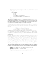
The wf predicate formalizes this description:
primrec wf where
“wf Λ = True” |
30
“wf (N _ k t u) =
(if t = Λ then
k = 1 ∧ (u = Λ ∨ (level u = 1 ∧ left u = Λ ∧ right u = Λ))
else
wf t ∧ wf u ∧ u 6= Λ ∧ level t < k ∧ level u ≤ k
∧ level (right u) < k )”
Rebalancing the tree upon insertion and removal of elements is performed by
two auxiliary functions called skew and split, defined below:
primrec skew where
“skew Λ = Λ” |
“skew (N x k t u) =
(if t 6= Λ ∧ k = level t then
N (data t) k (left t) (N x k (right t) u)
else
N x k t u)”
primrec split where
“split Λ = Λ” |
“split (N x k t u) =
(if u 6= Λ ∧ k = level (right u) then
N (data u) (Suc k ) (N x k t (left u)) (right u)
else
N x k t u)”
Performing a skew or a split should have no impact on the set of elements
stored in the tree:
theorem dataset_skew_split:
“dataset (skew t) = dataset t”
“dataset (split t) = dataset t”
nitpick
Nitpick ran out of time after checking 9 of 10 scopes.
Furthermore, applying skew or split on a well-formed tree should not alter
the tree:
theorem wf_skew_split:
“wf t =⇒ skew t = t”
“wf t =⇒ split t = t”
nitpick
Nitpick found no counterexample.
31
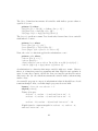
Insertion is implemented recursively. It preserves the sort order:
primrec insort where
“insort Λ x = N x 1 Λ Λ” |
“insort (N y k t u) x =
(∗ (split ◦ skew) ∗) (N y k (if x < y then insort t x else t)
(if x > y then insort u x else u))”
Notice that we deliberately commented out the application of skew and split.
Let’s see if this causes any problems:
theorem wf_insort: “wf t =⇒ wf (insort t x )”
nitpick
Nitpick found a counterexample for card 0 a = 4:
Free variables:
t = N a1 1 Λ Λ
x = a2
It’s hard to see why this is a counterexample. To improve readability, we
will restrict the theorem to nat, so that we don’t need to look up the value
of the op < constant to find out which element is smaller than the other. In
addition, we will tell Nitpick to display the value of insort t x using the eval
option. This gives
theorem wf_insort_nat: “wf t =⇒ wf (insort t (x ::nat))”
nitpick [eval = “insort t x ”]
Nitpick found a counterexample:
Free variables:
t =N 11ΛΛ
x =0
Evaluated term:
insort t x = N 1 1 (N 0 1 Λ Λ) Λ
Nitpick’s output reveals that the element 0 was added as a left child of
1, where both nodes have a level of 1. This violates the second AA tree
invariant, which states that a left child’s level must be less than its parent’s.
This shouldn’t come as a surprise, considering that we commented out the
tree rebalancing code. Reintroducing the code seems to solve the problem:
theorem wf_insort: “wf t =⇒ wf (insort t x )”
nitpick
Nitpick ran out of time after checking 8 of 10 scopes.
32
Insertion should transform the set of elements represented by the tree in the
obvious way:
theorem dataset_insort: “dataset (insort t x ) = {x } ∪ dataset t”
nitpick
Nitpick ran out of time after checking 7 of 10 scopes.
We could continue like this and sketch a full-blown theory of AA trees. Once
the definitions and main theorems are in place and have been thoroughly
tested using Nitpick, we could start working on the proofs. Developing theories this way usually saves time, because faulty theorems and definitions are
discovered much earlier in the process.
5
Option Reference
Nitpick’s behavior can be influenced by various options, which can be specified in brackets after the nitpick command. Default values can be set using
nitpick_params. For example:
nitpick_params [verbose, timeout = 60]
The options are categorized as follows: mode of operation (§5.1), scope of
search (§5.2), output format (§5.3), automatic counterexample checks (§5.4),
regression testing (§5.5), optimizations (§5.6), and timeouts (§5.7).
If you use Isabelle/jEdit, Nitpick also provides an automatic mode that can
be enabled via the “Auto Nitpick” option under “Plugins > Plugin Options >
Isabelle > General.” For automatic runs, user_axioms (§5.1), assms (§5.1),
and mono (§5.2) are implicitly enabled, blocking (§5.1), verbose (§5.3), and
debug (§5.3) are disabled, max_threads (§5.6) is taken to be 1, max_potential
(§5.3) is taken to be 0, and timeout (§5.7) is superseded by the “Auto Time
Limit” in jEdit. Nitpick’s output is also more concise.
The number of options can be overwhelming at first glance. Do not let that
worry you: Nitpick’s defaults have been chosen so that it almost always does
the right thing, and the most important options have been covered in context
in §3.
The descriptions below refer to the following syntactic quantities:
• hstring i: A string.
33
• hstring_listi: A space-separated list of strings (e.g., “ichi ni san”).
• hbool i: true or false.
• hsmart_bool i: true, false, or smart.
• hinti: An integer. Negative integers are prefixed with a hyphen.
• hsmart_inti: An integer or smart.
• hint_rangei: An integer (e.g., 3) or a range of nonnegative integers
(e.g., 1–4). The range symbol ‘–’ can be entered as - (hyphen) or
\<emdash>.
• hint_seq i: A comma-separated sequence of ranges of integers (e.g., 1,3,
6–8).
• hfloati: An floating-point number (e.g., 0.5 or 60) expressing a number
of seconds.
• hconsti: The name of a HOL constant.
• htermi: A HOL term (e.g., “f x ”).
• hterm_listi: A space-separated list of HOL terms (e.g., “f x ” “g y”).
• htypei: A HOL type.
Default values are indicated in curly brackets ({}). Boolean options have a
negated counterpart (e.g., blocking vs. non_blocking). When setting them,
“= true” may be omitted.
5.1
Mode of Operation
blocking = hbool i {true}
(neg.: non_blocking )
Specifies whether the nitpick command should operate synchronously.
The asynchronous (non-blocking) mode lets the user start proving the
putative theorem while Nitpick looks for a counterexample, but it can
also be more confusing. For technical reasons, automatic runs currently
always block.
falsify = hbool i {true}
(neg.: satisfy )
Specifies whether Nitpick should look for falsifying examples (countermodels) or satisfying examples (models). This manual assumes
throughout that falsify is enabled.
34
user_axioms = hsmart_bool i {smart} (neg.: no_user_axioms)
Specifies whether the user-defined axioms (specified using axiomatization and axioms) should be considered. If the option is set to smart,
Nitpick performs an ad hoc axiom selection based on the constants that
occur in the formula to falsify. The option is implicitly set to true for
automatic runs.
Warning: If the option is set to true, Nitpick might nonetheless ignore
some polymorphic axioms. Counterexamples generated under these
conditions are tagged as “quasi genuine.” The debug (§5.3) option can
be used to find out which axioms were considered.
See also assms (§5.1) and debug (§5.3).
assms = hbool i {true}
(neg.: no_assms)
Specifies whether the relevant assumptions in structured proofs should
be considered. The option is implicitly enabled for automatic runs.
See also user_axioms (§5.1).
spy = hbool i {false}
(neg.: dont_spy )
Specifies whether Nitpick should record statistics in $ISABELLE_HOME_
USER/spy_nitpick. These statistics can be useful to the developer of
Nitpick. If you are willing to have your interactions recorded in the
name of science, please enable this feature and send the statistics file
every now and then to the author of this manual (blannospam
chette@in.
tum.de). To change the default value of this option globally, set the
environment variable NITPICK_SPY to yes.
See also debug (§5.3).
overlord = hbool i {false}
(neg.: no_overlord )
Specifies whether Nitpick should put its temporary files in $ISABELLE_
HOME_USER, which is useful for debugging Nitpick but also unsafe if several instances of the tool are run simultaneously. The files are identified
by the extensions .kki, .cnf, .out, and .err; you may safely remove
them after Nitpick has run.
Warning: This option is not thread-safe. Use at your own risks.
See also debug (§5.3).
35
5.2
Scope of Search
card htypei = hint_seq i
Specifies the sequence of cardinalities to use for a given type. For free
types, and often also for typedecl’d types, it usually makes sense to
specify cardinalities as a range of the form 1–n.
See also box (§5.2) and mono (§5.2).
card = hint_seq i {1–10}
Specifies the default sequence of cardinalities to use. This can be overridden on a per-type basis using the card htypei option described above.
max hconsti = hint_seq i
Specifies the sequence of maximum multiplicities to use for a given
(co)inductive datatype constructor. A constructor’s multiplicity is the
number of distinct values that it can construct. Nonsensical values
(e.g., max [] = 2) are silently repaired. This option is only available for
datatypes equipped with several constructors.
max = hint_seq i
Specifies the default sequence of maximum multiplicities to use for
(co)inductive datatype constructors. This can be overridden on a perconstructor basis using the max hconsti option described above.
binary_ints = hsmart_bool i {smart}
(neg.: unary_ints)
Specifies whether natural numbers and integers should be encoded using a unary or binary notation. In unary mode, the cardinality fully
specifies the subset used to approximate the type. For example:
card nat = 4 induces
card int = 4 induces
card int = 5 induces
{0, 1, 2, 3}
{−1, 0, +1, +2}
{−2, −1, 0, +1, +2}.
In general:
card nat = K
card int = K
induces
induces
{0, . . . , K − 1}
{−dK /2e + 1, . . . , +bK /2c}.
In binary mode, the cardinality specifies the number of distinct values
that can be constructed. Each of these value is represented by a bit
pattern whose length is specified by the bits (§5.2) option. By default,
36
Nitpick attempts to choose the more appropriate encoding by inspecting the formula at hand, preferring the binary notation for problems
involving multiplicative operators or large constants.
Warning: For technical reasons, Nitpick always reverts to unary for
problems that refer to the types rat or real or the constants Suc, gcd,
or lcm.
See also bits (§5.2) and show_types (§5.3).
bits = hint_seq i {1–10}
Specifies the number of bits to use to represent natural numbers and
integers in binary, excluding the sign bit. The minimum is 1 and the
maximum is 31.
See also binary_ints (§5.2).
wf hconsti = hsmart_bool i
(neg.: non_wf )
Specifies whether the specified (co)inductively defined predicate is wellfounded. The option can take the following values:
• true: Tentatively treat the (co)inductive predicate as if it were
well-founded. Since this is generally not sound when the predicate is not well-founded, the counterexamples are tagged as “quasi
genuine.”
• false: Treat the (co)inductive predicate as if it were not well-
founded. The predicate is then unrolled as prescribed by the
star_linear_preds, iter hconsti, and iter options.
• smart: Try to prove that the inductive predicate is well-founded
using Isabelle’s lexicographic_order and size_change tactics. If
this succeeds (or the predicate occurs with an appropriate polarity
in the formula to falsify), use an efficient fixed-point equation
as specification of the predicate; otherwise, unroll the predicates
according to the iter hconsti and iter options.
See also iter (§5.2), star_linear_preds (§5.6), and tac_timeout (§5.7).
wf = hsmart_bool i {smart}
(neg.: non_wf )
Specifies the default wellfoundedness setting to use. This can be overridden on a per-predicate basis using the wf hconsti option above.
iter hconsti = hint_seq i
Specifies the sequence of iteration counts to use when unrolling a given
(co)inductive predicate. By default, unrolling is applied for inductive
37
predicates that occur negatively and coinductive predicates that occur
positively in the formula to falsify and that cannot be proved to be
well-founded, but this behavior is influenced by the wf option. The
iteration counts are automatically bounded by the cardinality of the
predicate’s domain.
See also wf (§5.2) and star_linear_preds (§5.6).
iter = hint_seq i {0,1,2,4,8,12,16,20,24,28}
Specifies the sequence of iteration counts to use when unrolling (co)inductive predicates. This can be overridden on a per-predicate basis
using the iter hconsti option above.
bisim_depth = hint_seq i {9}
Specifies the sequence of iteration counts to use when unrolling the
bisimilarity predicate generated by Nitpick for coinductive datatypes.
A value of −1 means that no predicate is generated, in which case Nitpick performs an after-the-fact check to see if the known coinductive
datatype values are bidissimilar. If two values are found to be bisimilar, the counterexample is tagged as “quasi genuine.” The iteration
counts are automatically bounded by the sum of the cardinalities of
the coinductive datatypes occurring in the formula to falsify.
box htypei = hsmart_bool i
(neg.: dont_box )
Specifies whether Nitpick should attempt to wrap (“box”) a given function or product type in an isomorphic datatype internally. Boxing is
an effective mean to reduce the search space and speed up Nitpick,
because the isomorphic datatype is approximated by a subset of the
possible function or pair values. Like other drastic optimizations, it
can also prevent the discovery of counterexamples. The option can
take the following values:
• true: Box the specified type whenever practicable.
• false: Never box the type.
• smart: Box the type only in contexts where it is likely to help.
For example, n-tuples where n > 2 and arguments to higher-order
functions are good candidates for boxing.
See also finitize (§5.2), verbose (§5.3), and debug (§5.3).
box = hsmart_bool i {smart}
(neg.: dont_box )
Specifies the default boxing setting to use. This can be overridden on
a per-type basis using the box htypei option described above.
38
finitize htypei = hsmart_bool i
(neg.: dont_finitize)
Specifies whether Nitpick should attempt to finitize an infinite datatype. The option can then take the following values:
• true: Finitize the datatype.
Since this is unsound, counterexamples generated under these conditions are tagged as “quasi
genuine.”
• false: Don’t attempt to finitize the datatype.
• smart: If the datatype’s constructors don’t appear in the prob-
lem, perform a monotonicity analysis to detect whether the datatype can be soundly finitized; otherwise, don’t finitize it.
See also box (§5.2), mono (§5.2), verbose (§5.3), and debug (§5.3).
finitize = hsmart_bool i {smart}
(neg.: dont_finitize)
Specifies the default finitization setting to use. This can be overridden
on a per-type basis using the finitize htypei option described above.
mono htypei = hsmart_bool i
(neg.: non_mono)
Specifies whether the given type should be considered monotonic when
enumerating scopes and finitizing types. If the option is set to smart,
Nitpick performs a monotonicity check on the type. Setting this option
to true can reduce the number of scopes tried, but it can also diminish
the chance of finding a counterexample, as demonstrated in §3.11. The
option is implicitly set to true for automatic runs.
See also card (§5.2), finitize (§5.2), merge_type_vars (§5.2), and verbose
(§5.3).
mono = hsmart_bool i {smart}
(neg.: non_mono)
Specifies the default monotonicity setting to use. This can be overridden on a per-type basis using the mono htypei option described above.
merge_type_vars = hbool i {false}
(neg.:
dont_merge_type_vars)
Specifies whether type variables with the same sort constraints should
be merged. Setting this option to true can reduce the number of scopes
tried and the size of the generated Kodkod formulas, but it also diminishes the theoretical chance of finding a counterexample.
See also mono (§5.2).
39
5.3
Output Format
verbose = hbool i {false}
(neg.: quiet)
Specifies whether the nitpick command should explain what it does.
This option is useful to determine which scopes are tried or which SAT
solver is used. This option is implicitly disabled for automatic runs.
debug = hbool i {false}
(neg.: no_debug )
Specifies whether Nitpick should display additional debugging information beyond what verbose already displays. Enabling debug also
enables verbose and show_all behind the scenes. The debug option is
implicitly disabled for automatic runs.
See also spy (§5.1), overlord (§5.1), and batch_size (§5.6).
show_types = hbool i {false}
(neg.: hide_types)
Specifies whether the subsets used to approximate (co)inductive datatypes should be displayed as part of counterexamples. Such subsets are
sometimes helpful when investigating whether a potentially spurious
counterexample is genuine, but their potential for clutter is real.
show_skolems = hbool i {true}
(neg.: hide_skolem)
Specifies whether the values of Skolem constants should be displayed
as part of counterexamples. Skolem constants correspond to bound
variables in the original formula and usually help us to understand
why the counterexample falsifies the formula.
show_consts = hbool i {false}
(neg.: hide_consts)
Specifies whether the values of constants occurring in the formula (including its axioms) should be displayed along with any counterexample.
These values are sometimes helpful when investigating why a counterexample is genuine, but they can clutter the output.
show_all = hbool i
Abbreviation for show_types, show_skolems, and show_consts.
max_potential = hinti {1}
Specifies the maximum number of potentially spurious counterexamples
to display. Setting this option to 0 speeds up the search for a genuine
counterexample. This option is implicitly set to 0 for automatic runs.
40
If you set this option to a value greater than 1, you will need an incremental SAT solver, such as MiniSat_JNI (recommended) and SAT4J.
Be aware that many of the counterexamples may be identical.
See also check_potential (§5.4) and sat_solver (§5.6).
max_genuine = hinti {1}
Specifies the maximum number of genuine counterexamples to display.
If you set this option to a value greater than 1, you will need an incremental SAT solver, such as MiniSat_JNI (recommended) and SAT4J.
Be aware that many of the counterexamples may be identical.
See also check_genuine (§5.4) and sat_solver (§5.6).
eval = hterm_listi
Specifies the list of terms whose values should be displayed along with
counterexamples. This option suffers from an “observer effect”: Nitpick
might find different counterexamples for different values of this option.
atoms htypei = hstring_listi
Specifies the names to use to refer to the atoms of the given type. By
default, Nitpick generates names of the form a1 , . . . , an , where a is the
first letter of the type’s name.
atoms = hstring_listi
Specifies the default names to use to refer to atoms of any type. For
example, to call the three atoms of type 0 a ichi, ni, and san instead
of a1 , a2 , a3 , specify the option “atoms 0 a = ichi ni san”. The default
names can be overridden on a per-type basis using the atoms htypei
option described above.
format htermi = hint_seq i
Specifies how to uncurry the value displayed for a variable or constant.
Uncurrying sometimes increases the readability of the output for higharity functions. For example, given the variable y :: 0 a ⇒ 0 b ⇒ 0 c ⇒
0
d ⇒ 0 e ⇒ 0 f ⇒ 0 g, setting format y = 3 tells Nitpick to group the last
three arguments, as if the type had been 0 a ⇒ 0 b ⇒ 0 c ⇒ 0 d × 0 e × 0 f ⇒
0
g. In general, a list of values n1 , . . . , nk tells Nitpick to show the last
nk arguments as an nk -tuple, the previous nk −1 arguments as an nk −1 tuple, and so on; arguments that are not accounted for are left alone,
as if the specification had been 1, . . . , 1, n1 , . . . , nk .
41
format = hint_seq i {1}
Specifies the default format to use. Irrespective of the default format,
the extra arguments to a Skolem constant corresponding to the outer
bound variables are kept separated from the remaining arguments, the
for arguments of an inductive definitions are kept separated from the
remaining arguments, and the iteration counter of an unrolled inductive
definition is shown alone. The default format can be overridden on
a per-variable or per-constant basis using the format htermi option
described above.
5.4
Authentication
check_potential = hbool i {false}
(neg.: trust_potential )
Specifies whether potentially spurious counterexamples should be given
to Isabelle’s auto tactic to assess their validity. If a potentially spurious
counterexample is shown to be genuine, Nitpick displays a message to
this effect and terminates.
See also max_potential (§5.3).
check_genuine = hbool i {false}
(neg.: trust_genuine)
Specifies whether genuine and quasi genuine counterexamples should
be given to Isabelle’s auto tactic to assess their validity. If a “genuine”
counterexample is shown to be spurious, the user is kindly asked to
send a bug report to the author at blannospam
[email protected].
See also max_genuine (§5.3).
5.5
Regression Testing
expect = hstring i
Specifies the expected outcome, which must be one of the following:
• genuine: Nitpick found a genuine counterexample.
• quasi_genuine: Nitpick found a “quasi genuine” counterexample
(i.e., a counterexample that is genuine unless it contradicts a missing axiom or a dangerous option was used inappropriately).
• potential : Nitpick found a potentially spurious counterexample.
• none: Nitpick found no counterexample.
42
• unknown: Nitpick encountered some problem (e.g., Kodkod ran
out of memory).
Nitpick emits an error if the actual outcome differs from the expected
outcome. This option is useful for regression testing.
5.6
Optimizations
sat_solver = hstring i {smart}
Specifies which SAT solver to use. SAT solvers implemented in C or
C++ tend to be faster than their Java counterparts, but they can be
more difficult to install. Also, if you set the max_potential (§5.3) or
max_genuine (§5.3) option to a value greater than 1, you will need
an incremental SAT solver, such as MiniSat_JNI (recommended) or
SAT4J.
The supported solvers are listed below:
• Lingeling_JNI : Lingeling is an efficient solver written in C. The
JNI (Java Native Interface) version of Lingeling is bundled with
Kodkodi and is precompiled for Linux and Mac OS X. It is also
available from the Kodkod web site [6].
• CryptoMiniSat:
CryptoMiniSat is the winner of the 2010
SAT Race. To use CryptoMiniSat, set the environment variable CRYPTOMINISAT_HOME to the directory that contains the
cryptominisat executable.3 The C++ sources and executables
for CryptoMiniSat are available at http://planete.inrialpes.
fr/~soos/CryptoMiniSat2/index.php. Nitpick has been tested
with version 2.51.
• CryptoMiniSat_JNI : The JNI (Java Native Interface) version
of CryptoMiniSat is bundled with Kodkodi and is precompiled for
Linux and Mac OS X. It is also available from the Kodkod web
site [6].
• MiniSat: MiniSat is an efficient solver written in C++. To use
MiniSat, set the environment variable MINISAT_HOME to the directory that contains the minisat executable.3 The C++ sources
and executables for MiniSat are available at http://minisat.se/
MiniSat.html. Nitpick has been tested with versions 1.14 and 2.2.
3
Important note for Cygwin users: The path must be specified using native Windows
syntax. Make sure to escape backslashes properly.
43
• MiniSat_JNI : The JNI version of MiniSat is bundled with Kod-
kodi and is precompiled for Linux, Mac OS X, and Windows (Cygwin). It is also available from the Kodkod web site [6]. Unlike the
standard version of MiniSat, the JNI version can be used incrementally.
• Riss3g : Riss3g is an efficient solver written in C++. To use
Riss3g, set the environment variable RISS3G_HOME to the directory that contains the riss3g executable.3 The C++ sources
for Riss3g are available at http://tools.computational-logic.
org/content/riss3g.php. Nitpick has been tested with the SAT
Competition 2013 version.
• zChaff : zChaff is an older solver written in C++.
To use
zChaff, set the environment variable ZCHAFF_HOME to the directory that contains the zchaff executable.3 The C++ sources and
executables for zChaff are available at http://www.princeton.
edu/~chaff/zchaff.html. Nitpick has been tested with versions
2004-05-13, 2004-11-15, and 2007-03-12.
• RSat: RSat is an efficient solver written in C++. To use RSat, set
the environment variable RSAT_HOME to the directory that contains
the rsat executable.3 The C++ sources for RSat are available
at http://reasoning.cs.ucla.edu/rsat/. Nitpick has been
tested with version 2.01.
• BerkMin: BerkMin561 is an efficient solver written in C. To use
BerkMin, set the environment variable BERKMIN_HOME to the directory that contains the BerkMin561 executable.3 The BerkMin executables are available at http://eigold.tripod.com/BerkMin.
html.
• BerkMin_Alloy : Variant of BerkMin that is included with Al-
loy 4 and calls itself “sat56” in its banner text. To use this version
of BerkMin, set the environment variable BERKMINALLOY_HOME to
the directory that contains the berkmin executable.3
• SAT4J : SAT4J is a reasonably efficient solver written in Java
that can be used incrementally. It is bundled with Kodkodi and
requires no further installation or configuration steps. Do not
attempt to install the official SAT4J packages, because their API
is incompatible with Kodkod.
• SAT4J_Light: Variant of SAT4J that is optimized for small
problems. It can also be used incrementally.
44
• smart: If sat_solver is set to smart, Nitpick selects the first solver
among the above that is recognized by Isabelle. If verbose (§5.3)
is enabled, Nitpick displays which SAT solver was chosen.
batch_size = hsmart_inti {smart}
Specifies the maximum number of Kodkod problems that should be
lumped together when invoking Kodkodi. Each problem corresponds
to one scope. Lumping problems together ensures that Kodkodi is
launched less often, but it makes the verbose output less readable and
is sometimes detrimental to performance. If batch_size is set to smart,
the actual value used is 1 if debug (§5.3) is set and 50 otherwise.
destroy_constrs = hbool i {true} (neg.: dont_destroy_constrs)
Specifies whether formulas involving (co)inductive datatype constructors should be rewritten to use (automatically generated) discriminators and destructors. This optimization can drastically reduce the size
of the Boolean formulas given to the SAT solver.
See also debug (§5.3).
specialize = hbool i {true}
(neg.: dont_specialize)
Specifies whether functions invoked with static arguments should be
specialized. This optimization can drastically reduce the search space,
especially for higher-order functions.
See also debug (§5.3) and show_consts (§5.3).
star_linear_preds = hbool i {true}
dont_star_linear_preds)
(neg.:
Specifies whether Nitpick should use Kodkod’s transitive closure operator to encode non-well-founded “linear inductive predicates,” i.e.,
inductive predicates for which each the predicate occurs in at most one
assumption of each introduction rule. Using the reflexive transitive closure is in principle equivalent to setting iter to the cardinality of the
predicate’s domain, but it is usually more efficient.
See also wf (§5.2), debug (§5.3), and iter (§5.2).
whack = hterm_listi
Specifies a list of atomic terms (usually constants, but also free and
schematic variables) that should be taken as being _ (unknown). This
can be useful to reduce the size of the Kodkod problem if you can guess
in advance that a constant might not be needed to find a countermodel.
45
See also debug (§5.3).
need = hterm_listi
Specifies a list of datatype values (normally ground constructor terms)
that should be part of the subterm-closed subsets used to approximate
datatypes. If you know that a value must necessarily belong to the
subset of representable values that approximates a datatype, specifying
it can speed up the search, especially for high cardinalities.
total_consts = hsmart_bool i {smart}
(neg.: partial_consts)
Specifies whether constants occurring in the problem other than constructors can be assumed to be considered total for the representable
values that approximate a datatype. This option is highly incomplete;
it should be used only for problems that do not construct datatype
values explicitly. Since this option is (in rare cases) unsound, counterexamples generated under these conditions are tagged as “quasi genuine.”
datatype_sym_break = hinti {5}
Specifies an upper bound on the number of datatypes for which Nitpick generates symmetry breaking predicates. Symmetry breaking can
speed up the SAT solver considerably, especially for unsatisfiable problems, but too much of it can slow it down.
kodkod_sym_break = hinti {15}
Specifies an upper bound on the number of relations for which Kodkod generates symmetry breaking predicates. Symmetry breaking can
speed up the SAT solver considerably, especially for unsatisfiable problems, but too much of it can slow it down.
peephole_optim = hbool i {true}
(neg.: no_peephole_optim)
Specifies whether Nitpick should simplify the generated Kodkod formulas using a peephole optimizer. These optimizations can make a
significant difference. Unless you are tracking down a bug in Nitpick or
distrust the peephole optimizer, you should leave this option enabled.
max_threads = hinti {0}
Specifies the maximum number of threads to use in Kodkod. If this
option is set to 0, Kodkod will compute an appropriate value based on
the number of processor cores available. The option is implicitly set to
1 for automatic runs.
See also batch_size (§5.6) and timeout (§5.7).
46
5.7
Timeouts
timeout = hfloati {30}
Specifies the maximum number of seconds that the nitpick command
should spend looking for a counterexample. Nitpick tries to honor this
constraint as well as it can but offers no guarantees. For automatic
runs, the “Auto Time Limit” option under “Plugins > Plugin Options
> Isabelle > General” is used instead.
See also max_threads (§5.6).
tac_timeout = hfloati {0.5}
Specifies the maximum number of seconds that should be used by
internal tactics—lexicographic_order and size_change when checking
whether a (co)inductive predicate is well-founded, auto tactic when
checking a counterexample, or the monotonicity inference. Nitpick tries
to honor this constraint but offers no guarantees.
See also wf (§5.2), mono (§5.2), check_potential (§5.4), and check_genuine
(§5.4).
6
Attribute Reference
Nitpick needs to consider the definitions of all constants occurring in a formula in order to falsify it. For constants introduced using the definition
command, the definition is simply the associated _def axiom. In contrast,
instead of using the internal representation of functions synthesized by Isabelle’s primrec, function, and nominal_primrec packages, Nitpick relies
on the more natural equational specification entered by the user.
Behind the scenes, Isabelle’s built-in packages and theories rely on the following attributes to affect Nitpick’s behavior:
nitpick_unfold
This attribute specifies an equation that Nitpick should use to expand a
constant. The equation should be logically equivalent to the constant’s
actual definition and should be of the form
c ?x1 . . . ?xn = t,
or
c ?x1 . . . ?xn ≡ t,
47
where ?x1 , . . . , ?xn are distinct variables and c does not occur in t. Each
occurrence of c in the problem is expanded to λx1 . . . xn . t.
nitpick_simp
This attribute specifies the equations that constitute the specification
of a constant. The primrec, function, and nominal_primrec packages automatically attach this attribute to their simps rules. The equations must be of the form
c t1 . . . tn = u
or
c t1 . . . tn ≡ u.
nitpick_psimp
This attribute specifies the equations that constitute the partial specification of a constant. The function package automatically attaches
this attribute to its psimps rules. The conditional equations must be
of the form
[[P1 ; . . . ; Pm ]] =⇒ c t1 . . . tn = u
or
[[P1 ; . . . ; Pm ]] =⇒ c t1 . . . tn ≡ u.
nitpick_choice_spec
This attribute specifies the (free-form) specification of a constant defined using the (ax_)specification command.
When faced with a constant, Nitpick proceeds as follows:
1. If the nitpick_simp set associated with the constant is not empty, Nitpick uses these rules as the specification of the constant.
2. Otherwise, if the nitpick_psimp set associated with the constant is not
empty, it uses these rules as the specification of the constant.
3. Otherwise, if the constant was defined using the (ax_)specification
command and the nitpick_choice_spec set associated with the constant
is not empty, it uses these theorems as the specification of the constant.
4. Otherwise, it looks up the definition of the constant.
If the
nitpick_unfold set associated with the constant is not empty, it uses the
latest rule added to the set as the definition of the constant; otherwise
it uses the actual definition axiom.
48
1. If the definition is of the form
c ?x1 . . . ?xm ≡ λy1 . . . yn . lfp (λf . t)
or
c ?x1 . . . ?xm ≡ λy1 . . . yn . gfp (λf . t).
Nitpick assumes that the definition was made using a (co)inductive
package based on the user-specified introduction rules registered
in Isabelle’s internal Spec_Rules table. The tool uses the introduction rules to ascertain whether the definition is well-founded
and the definition to generate a fixed-point equation or an unrolled
equation.
2. If the definition is compact enough, the constant is unfolded wherever it appears; otherwise, it is defined equationally, as with the
nitpick_simp attribute.
As an illustration, consider the inductive definition
inductive odd where
“odd 1” |
“odd n =⇒ odd (Suc (Suc n))”
By default, Nitpick uses the lfp-based definition in conjunction with the
introduction rules. To override this, you can specify an alternative definition
as follows:
lemma odd _alt_unfold [nitpick_unfold ]: “odd n ≡ n mod 2 = 1”
Nitpick then expands all occurrences of odd n to n mod 2 = 1. Alternatively,
you can specify an equational specification of the constant:
lemma odd _simp [nitpick_simp]: “odd n = (n mod 2 = 1)”
Such tweaks should be done with great care, because Nitpick will assume
that the constant is completely defined by its equational specification. For
example, if you make “odd (2 ∗ k + 1)” a nitpick_simp rule and neglect to
provide rules to handle the 2 ∗ k case, Nitpick will define odd n arbitrarily for
even values of n. The debug (§5.3) option is extremely useful to understand
what is going on when experimenting with nitpick_ attributes.
Because of its internal three-valued logic, Nitpick tends to lose a lot of precision in the presence of partially specified constants. For example,
lemma odd_simp [nitpick_simp]: “odd x = ¬ even x ”
is superior to
49
lemma odd_psimps [nitpick_simp]:
“even x =⇒ odd x = False”
“¬ even x =⇒ odd x = True”
Because Nitpick sometimes unfolds definitions but never simplification rules,
you can ensure that a constant is defined explicitly using the nitpick_simp.
For example:
definition optimum where [nitpick_simp]:
“optimum t = (∀u. consistent u ∧ alphabet t = alphabet u
∧ freq t = freq u −→ cost t ≤ cost u)”
In some rare occasions, you might want to provide an inductive or coinductive
view on top of an existing constant c. The easiest way to achieve this is to
define a new constant c 0 (co)inductively. Then prove that c equals c 0 and let
Nitpick know about it:
lemma c_alt_unfold [nitpick_unfold ]: “c ≡ c 0 ”
This ensures that Nitpick will substitute c 0 for c and use the (co)inductive
definition.
7
Standard ML Interface
Nitpick provides a rich Standard ML interface used mainly for internal purposes and debugging. Among the most interesting functions exported by
Nitpick are those that let you invoke the tool programmatically and those
that let you register and unregister custom term postprocessors as well as
coinductive datatypes.
7.1
Invoking Nitpick
The Nitpick structure offers the following functions for invoking your favorite
counterexample generator:
val pick_nits_in_term :
Proof.state → params → mode → int → int → int
→ (term ∗ term) list → term list → term → string ∗ Proof.state
val pick_nits_in_subgoal :
Proof.state → params → mode → int → int → string ∗ Proof.state
50
The return value is a new proof state paired with an outcome string (“genuine”, “quasi_genuine”, “potential”, “none”, or “unknown”). The params type
is a large record that lets you set Nitpick’s options. The current default
options can be retrieved by calling the following function defined in the
Nitpick_Isar structure:
val default_params : theory → (string ∗ string) list → params
The second argument lets you override option values before they are parsed
and put into a params record. Here is an example where Nitpick is invoked
on subgoal i of n with no time limit:
val params = Nitpick_Isar.default_params thy [(“timeout”, “none”)]
val (outcome, state0 ) =
Nitpick.pick_nits_in_subgoal state params Nitpick.Normal i n
7.2
Registering Term Postprocessors
It is possible to change the output of any term that Nitpick considers a
datatype by registering a term postprocessor. The interface for registering
and unregistering postprocessors consists of the following pair of functions
defined in the Nitpick_Model structure:
type term_postprocessor =
Proof.context → string → (typ → term list) → typ → term → term
val register_term_postprocessor :
typ → term_postprocessor → morphism → Context.generic
→ Context.generic
val unregister_term_postprocessor :
typ → morphism → Context.generic → Context.generic
§3.7 and src/HOL/Library/Multiset.thy illustrate this feature in context.
7.3
Registering Coinductive Datatypes
Coinductive datatypes defined using the codatatype command that do not
involve nested recursion through non-codatatypes are supported by Nitpick.
If you have defined a custom coinductive datatype, you can tell Nitpick about
it, so that it can use an efficient Kodkod axiomatization. The interface for
registering and unregistering coinductive datatypes consists of the following
pair of functions defined in the Nitpick_HOL structure:
51
val register_codatatype :
morphism → typ → string → (string × typ) list → Context.generic
→ Context.generic
val unregister_codatatype :
morphism → typ → Context.generic → Context.generic
The type 0 a llist of lazy lists is already registered; had it not been, you could
have told Nitpick about it by adding the following line to your theory file:
declaration {∗
Nitpick_HOL.register_codatatype @{typ “ 0 a llist”}
@{const_name llist_case}
(map dest_Const [@{term LNil}, @{term LCons}])
∗}
The register_codatatype function takes a coinductive datatype, its case function, and the list of its constructors (in addition to the current morphism
and generic proof context). The case function must take its arguments in the
order that the constructors are listed. If no case function with the correct
signature is available, simply pass the empty string.
On the other hand, if your goal is to cripple Nitpick, add the following line
to your theory file and try to check a few conjectures about lazy lists:
declaration {∗
Nitpick_HOL.unregister_codatatype @{typ “ 0 a llist”}
∗}
Inductive datatypes can be registered as coinductive datatypes, given appropriate coinductive constructors. However, doing so precludes the use of the
inductive constructors—Nitpick will generate an error if they are needed.
8
Known Bugs and Limitations
Here are the known bugs and limitations in Nitpick at the time of writing:
• Underspecified functions defined using the primrec, function, or
nominal_primrec packages can lead Nitpick to generate spurious
counterexamples for theorems that refer to values for which the function is not defined. For example:
primrec prec where
“prec (Suc n) = n”
52
lemma “prec 0 = undefined ”
nitpick
Nitpick found a counterexample for card nat = 2:
Empty assignment
by (auto simp: prec_def )
Such theorems are generally considered bad style because they rely
on the internal representation of functions synthesized by Isabelle, an
implementation detail.
• Similarly, Nitpick might find spurious counterexamples for theorems
that rely on the use of the indefinite description operator internally by
specification and quot_type.
• Axioms or definitions that restrict the possible values of the undefined
constant or other partially specified built-in Isabelle constants (e.g.,
Abs_ and Rep_ constants) are in general ignored. Again, such nonconservative extensions are generally considered bad style.
• Nitpick produces spurious counterexamples when invoked after a guess
command in a structured proof.
• Datatypes defined using datatype_new and codatatypes defined
using codatatype that involve nested (co)recursion through non(co)datatypes are not properly supported and may result in spurious
counterexamples.
• The nitpick_xxx attributes and the Nitpick_xxx.register_yyy functions
can cause havoc if used improperly.
• Although this has never been observed, arbitrary theorem morphisms
could possibly confuse Nitpick, resulting in spurious counterexamples.
• All constants, types, free variables, and schematic variables whose
names start with Nitpick . are reserved for internal use.
References
[1] A. Andersson. Balanced search trees made simple. In F. K. H. A. Dehne,
N. Santoro, and S. Whitesides, editors, WADS 1993, volume 709 of Lecture Notes in Computer Science, pages 61–70. Springer-Verlag, 1993.
53
[2] S. Berghofer and T. Nipkow. Random testing in Isabelle/HOL. In J. Cuellar and Z. Liu, editors, SEFM 2004, pages 230–239. IEEE Computer
Society Press, 2004.
[3] J. C. Blanchette and T. Nipkow. Nitpick: A counterexample generator
for higher-order logic based on a relational model finder. In M. Kaufmann
and L. Paulson, editors, Interactive Theorem Proving: ITP-10, Lecture
Notes in Computer Science. Springer-Verlag, 2010.
[4] D. Jackson. Software Abstractions: Logic, Language, and Analysis. MIT
Press, 2006.
[5] T. Nipkow, L. C. Paulson, and M. Wenzel. Isabelle/HOL: A Proof Assistant for Higher-Order Logic, volume 2283 of Lecture Notes in Computer
Science. Springer-Verlag, 2002.
[6] E. Torlak. Kodkod: Constraint solver for relational logic. http://alloy.
mit.edu/kodkod/.
[7] E. Torlak and D. Jackson. Kodkod: A relational model finder. In
O. Grumberg and M. Huth, editors, TACAS 2007, volume 4424 of Lecture
Notes in Computer Science, pages 632–647. Springer-Verlag, 2007.
[8] T. Weber. SAT-Based Finite Model Generation for Higher-Order Logic.
Ph.D. thesis, Dept. of Informatics, T.U. München, 2008.
[9] Wikipedia: AA tree. http://en.wikipedia.org/wiki/AA_tree.
54