Download HIGH SPEED PHOTOMETER INSTRUMENT HANDBOOK

HIGH SPEED PHOTOMETER INSTRUMENT HANDBOOK
Version 3.0
April 1992
Robert C. Bless
Jerey W. Percival
University of Wisconsin
475 N. Charter Street, Madison, WI 53706
Lisa E. Walter
Richard L. White
Space Telescope Science Institute
3700 San Martin Drive, Baltimore, MD 21218
HSP Instrument Handbook Version 2.0
1
Chapter 1: Introduction
1.1 How to Use This Manual
This manual is a guide for astronomers who intend to use the High Speed Photometer (HSP),
one of the scientic instruments onboard the Hubble Space Telescope (HST). All the information
needed for ordinary uses of the HSP is contained in this manual, including:
(1) an overview of the instrument (Chapter 2),
(2) a detailed description of some details of the HSP-HST system that may be important
for some observations (Chapter 3),
(3) tables and gures describing the sensitivity and limitations of the HSP (Chapter 4),
(4) how to go about planning an observation with the HSP (Chapter 4), and
(5) a description of the standard calibrations to be applied to HSP data and the resulting
data products (Chapter 5).
An HSP neophyte should begin by reading Chapters 2 and 4 to get an overview of the instrument and what it can do. Chapter 4 also shows how to plan an observation using the HSP.
Chapter 5 describes the data products received by the observer. Skimming through Chapter 3 will
give some feeling for the complications that may arise.
The HSP sophisticate will refer mainly to Chapters 3 and 4, and may often nd that the
careful construction of complicated observing programs is driven by the constraints described in
Chapter 3.
Some observing programs will inevitably require more detailed information about the HSP
than is given here. For example, it is possible to write special purpose programs for a microprocessor inside the HSP that controls observing sequences, but this manual does not contain enough
information to determine precisely what can and cannot be done with such programs. If you require
such detailed information, it is available either from the Space Telescope Science Institute or from
the documents listed in the bibliography of this manual.
As time passes, there will undoubtedly be changes in this manual. Chapters 3 and 4 are
especially vulnerable to changing as our knowledge of the instrument improves. Consequently,
users should be wary of using outdated versions of the manual.
Suggestions for improvements are welcome and should be addressed to the authors.
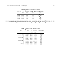
1.2 Acronyms
Acronyms are a necessary, if often overused, aid in reducing the length of NASA documents.
The following acronyms may rear their heads in this manual:
2
HSP Instrument Handbook Version 2.0
Table 1{1:
A/D
BD
CVZ
D/A
FGS
FOC
FOS
GSFC
GHRS
HSP
HST
IDT
NASA
NSSC-1
ODS
OTA
PAD
PDB
PMT
RAM
ROM
SCUM
SOGS
STScI
STSDAS
TAV
TBD
TDRSS
UV
WF/PC
Acronyms
Analog to Digital
Bus Director
Continuous Viewing Zone
Digital to Analog
Fine Guidance System
Faint Object Camera
Faint Object Spectrograph
Goddard Space Flight Center
Goddard High Resolution Spectrograph
High Speed Photometer
Hubble Space Telescope
Image Dissector Tube
National Aeronautics and Space Administration
NASA Standard Spacecraft Computer
Optical Detector Subsystem
Optical Telescope Assembly
Pulse Amplitude Discriminator
Project Data Base
Photomultiplier Tube
Random Access Memory
Read-Only Memory
System Controller User's Manual
Science Operations Ground System
Space Telescope Science Institute
Science Data Analysis System
Target Acquisition and Verication
To Be Determined
Tracking and Data Relay Satellite System
Ultraviolet
Wide Field/Planetary Camera
1.3 Acknowledgements
The High Speed Photometer was designed and built at the University of Wisconsin by Robert C.
Bless (Principal Investigator) with scientic guidance from the HSP Investigation Denition Team:
Joseph F. Dolan, James L. Elliott, Edward L. Robinson, and Wayne van Citters. Among those
making major contributions to the design, construction, and testing of the HSP were Evan Richards,
Je Percival, Fred Best, Dave Birdsall, Gene Buchholtz, Scott Ellington, Don Finegan, Ed Hatter,
Sally Laurent-Muehleisen, Matt Nelson, Bill Phillips, Jerry Sitzman, Mark Slovak, Colleen Townsley, Andrea Tui, Mark Werner, Doug Whiteley, and others, to whom I apologize for their omission
from this list.
Much useful criticism of the HSP Instrument Handbook was provided by Bob Bless, Joe
Dolan, Howard Bond, and Lisa Walter; however, any remaining problems are the responsibility of
the authors.
HSP Instrument Handbook Version 2.0
3
Chapter 2: Overview of the HSP
The High Speed Photometer (HSP) exploits the capabilities of the HST by making photometric
measurements over visual and ultraviolet (UV) wavelengths at rates up to 105 Hz and by measuring
very low amplitude variability (especially for hotter stars in the UV). A secondary purpose of the
instrument is to measure linear polarization in the near UV. The HSP has several advantages over
similar ground-based instruments:
(1) UV wavelength coverage.
(2) Smaller apertures, permitting higher spatial resolution and reducing the sky background.
(3) No atmospheric absorption or scintillation, leading to higher photometric accuracy
and the ability to use very short sample times.
In what follows we will present an overview of the HSP, its optics and detectors, its electronics,
its mechanical structure, and nally some observational considerations.
2.1 Summary of HSP Characteristics
Quantum Eciency:
Time Resolution:
0:1{3% (throughput for entire HSP-HST system)
10.7 s (pulse-counting mode, count rate < 106 cts/s)
1 ms (current mode, count rate > 106 cts/s)
Photometric Accuracy: Systematic errors < 2% from V=0 to V=20
Apertures:
1.0 arcsecond diameter for normal observations
6.0, 10.0 arcsecond for target acquisition
Filters:
23 UV and visual lters from 1200 A to 7500 A
Polarimetry:
4 UV lters
2% polarimetric accuracy
Operation:
Telescope must slew to move star from one lter to another.
Slew time 30{60 s (limits rate at which multicolor photometry is possible). There are four lter pairs with beamsplitters that can be used for two color photometry without
moving telescope; for these lter pairs, can get simultaneous
or nearly simultaneous (separated by only 10 milliseconds)
two color photometry.
a
2.2 Detectors and Optics Congurations
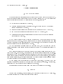
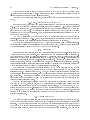
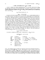
The HSP has quite an unusual design, in that it has no moving parts. Figure 2-1 shows a
sketch of the arrangement of the detectors and optics in the HSP. There are ve detectors in the
instrument|four image dissector tubes (IDTs) and one photomultiplier tube. The former are ITT
A
4012RP Vidissectors, two with CsTe photocathodes on MgF2 faceplates (sensitive from 1200 to 3000 A) and two with bialkali cathodes on suprasil faceplates (sensitive from 1600 A to about
7000 A). Each image dissector tube, its voltage divider network, and its deection and focus coils are
all contained in a double magnetic shield within the housing. The photomultiplier is a Hamamatsu
R666S with a GaAs photocathode. Three of the image dissectors|the two CsTe tubes (called
UV1 and UV2) and one of the bialkali tubes (VIS)|are used for photometry. The second bialkali
dissector (POL) is used for polarimetry,* and a beamsplitter allows the photomultiplier (PMT)
along with the bialkali photometry dissector (VIS) to be used for simultaneous observations in two
* Note that the polarimeter also has one clear lter that can be used for photometry.
4
a
HSP Instrument Handbook Version 2.0
Figure 2{1:
HSP Optics and Detectors
colors (e.g., for occultations). For convenience, we will refer to the photometric, polarimetric, and
PMT \congurations", but in most respects the operation of the various detectors is identical.
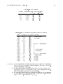
For the purposes of the HST proposal forms, the HSP has the following congurations and
modes:
Table 2{1:
Conguration
HSP Congurations and Modes
Modes
HSP/UV1, UV2, VIS SINGLE, STAR-SKY, ACQ, IMAGE, PRISM
HSP/POL
SINGLE, STAR-SKY, ACQ, IMAGE
HSP/PMT
SINGLE
HSP/hD1 i/hD2i
STAR-SKY
HSP/PMT/VIS
SPLIT
All these modes are discussed in the following paragraphs. The ACQ mode is used for target
acquisition and is also discussed in x2.5.1 and in the HSP Target Acquisition Handbook. See the
Hubble Space Telescope Phase II Proposal Instructions for information about how to specify the
various congurations and modes on the proposal forms.
2.2.1 Single-Color Photometry
Consider rst photometric observations, which can be carried out using the mode SINGLE. This
mode can be used with any of the ve HSP detectors. Light from the HST enters the HSP through
HSP Instrument Handbook Version 2.0
Figure 2{2:
5
HSP Focal Plane Layout
one of three holes in its forward bulkhead. These holes are all centered on an arc 8.1 arcminutes
o-axis; the focal plane layout for the HSP is shown in Figure 2-2. After passing through a lter
(which is about 36 mm in front of the HST focal plane) and an aperture (which is in the HST focal
plane), the light is brought to a refocus on the dissector photocathode by a relay mirror|a 60 mm
diameter o-axis ellipsoid located about 800 mm behind the HST focal surface. The relay mirrors
enable a more ecient use to be made of the HST focal plane available to the HSP than would
otherwise be possible, i.e., the image dissectors are too large to place more than two directly in the
focal plane. The magnication of the relay mirrors is about 0.65, which converts the f/24 bundle
entering the HSP to f/15.6 at the photocathode, with a corresponding change in scale from 3.58
arcseconds/mm to 5.54 arcseconds/mm.
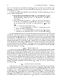
The only unusual feature of the HSP's optical system is its lter-aperture \mechanism" (see
Figures 2-3 through 2-7) mounted behind each forward bulkhead entrance hole. Each lter plate
contains thirteen lters mounted in two columns positioned 36 mm ahead of the HST focal plane.
At this location the converging bundle of light from the HST is 1.5 mm in diameter, well within
the 3 mm width of each lter; however, because the light bundle is out of focus, small variations in
lter transmission with position should not be important. For each lter plate there is an aperture
plate, located at the HST focal surface, that contains 48 apertures arranged in two columns that are
positioned directly behind the corresponding columns of lters. Nine of the lters are associated
with four apertures each|two with diameters of 1 arcsecond (280 m) and two with diameters
of 0.4 arcseconds (112 m). Due to space limitations, one lter is associated with only three
apertures, and two other lters are associated with two apertures each. The thirteenth lter, of
double width, is a clear window and has ve associated apertures, including one of 10 arcsecond
diameter for target acquisition. The VIS detector has one additional aperture that also passes light
to the PMT (see x2.2.3). The choice of 1.0 and 0.4 arcsecond apertures was made on the basis of
6
HSP Instrument Handbook Version 2.0
the specied performance of the HST image at the HSP location 8 arcminutes o-axis. However,
the degraded image caused by spherical aberration severely limits the utility of the 0.4 arcsecond
apertures because the amount of energy encircled is only 20% of that expected. Normally, therefore,
the 1.0 arcsecond apertures will be used for most observations.
The HST is commanded to point so that the target's position in the HST focal plane coincides
with the particular lter-aperture combination desired. Light from the target is then focused on
the dissector cathode by the relay mirror. The resulting photoelectrons are magnetically focused
and deected in the forward section of the image dissector so that the photocurrent is directed
through a 180 m aperture (corresponding to 1 arcsecond on the sky). This aperture connects the
forward section of the detector to a 12-stage photomultiplier section. Thus with no moving parts,
48 dierent lter-aperture combinations are available for each photometry detector in the HSP.
Not all of these are unique, however, because of duplicate lters and duplicate apertures associated
with each lter.
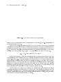
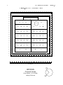
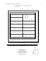
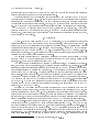
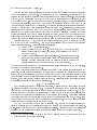
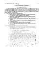
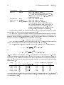
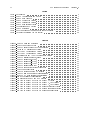
The following series of four charts (Figures 2-3 through 2-7) show the lter and aperture
conguration for the four HSP images dissector tubes. On the left side of each lter strip from top
to bottom, the following information is provided:
(1) The lter designation in PDB syntax.
(2) The (obsolete) original HSP team lter designation, provided for reference
to old documentation only.
(3) The lter designation in current proposal syntax.
For each aperture, the following information is provided from top to bottom:
(1) The aperture designation in PDB syntax.
(2) The (obsolete) original HSP team aperture designation, provided for reference to old documentation only.
(3) The aperture designation in current proposal syntax.
There are three so-called \dark apertures" on each IDT that are labeled D1, D2, and D3.
These \apertures" represent the locations on the solid part of the faceplate to where the readbeam
is deected for collection of dark counts. The innermost scale is the physical scale in millimeters of
the lters and apertures referenced to the image dissector tube faceplate. The deection step scale
represents the magnetic deection (in HSP D/A units) required to point the read beam to any
location. These are provided as reference only and are not used in proposals. The outermost scale
is in arcseconds and is referenced to the focal plane. The V2 and V3 axes are shown relative to the
position of the detectors as projected through the optics onto the sky. The order of the scales for
the POL diagram (Figure 2-7) is slightly dierent.
All of the UV lters are multi-layer interference lters of Al and MgF2 evaporated on MgF2
substrates for the far ultraviolet, or on suprasil for the near UV. The visual lters consist of Ag and
cryolite layers deposited on glass. The substrates are 1/16 inch (60:002 inch) thick. The general
lter characteristics are listed below in Tables 4-1 and 4-2. Some lters are common to two or more
photometry image dissectors for the sake of redundancy and to enable all three channels to be tied
together photometrically. Some lters dene bandpasses similar to those own on previous space
observatories, while others are similar to some in the Wide Field and Faint Object Cameras.
There is one lter on the POL IDT (F160LP, see Fig. 2-7) with two 0.65 arcsecond apertures
that can be used for photometry. The other lters on POL have polarizers and can be used only
for polarimetry (x2.2.4).
Figure 2-2 shows the X and Y reference axes that are used if it is necessary to specify a
particular orientation for an HSP observation (using the ORIENT special requirement) or a special
position for a target in an aperture (using the POS TARG special requirement). For example, the
acceptable range of orientations may be restricted to insure that an aperture to be used for mea-
HSP Instrument Handbook Version 2.0
Figure 2{3:
7
HSP Filter/Aperture Tube Conguration
surement of the sky brightness will not be contaminated by eld star. (See x2.5.2 for discussion of
sky subtraction using the HSP.)
Notice that lter changes generally require the HST to slew from one aperture to another;
this requires about 30 seconds for two apertures on the same IDT and about 60 seconds for two
apertures on dierent IDTs. The slew time determines how rapidly multicolor photometry can be
done. There are two exceptions to this restriction: rapid two-color observations can be made either
in PRISM mode with detectors VIS, UV1, and UV2, or in SPLIT mode using PMT and VIS.
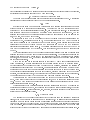
2.2.2 Two-Color Photometry with Prisms
On each photometry IDT, there is a beamsplitter/prism combination that divides the light of
an appropriately placed target between two 1 arcsecond apertures that have dierent lters (see
Figures 2-4 through 2-6). A partially reecting MgF2 plate mounted at 45 to the incoming beam
transmits part of the incident light to a lter and 1 arcsecond aperture. The reected beam is totally
internally reected by a right angle prism made of suprasil; it then passes through another lter, a
suprasil rod (which compensates for the longer path followed by the reected beam), and another
1 arcsecond aperture. In all cases, the transmitted beam passes through the short wavelength lter
and the reected beam goes through the long wavelength lter of the pair.
Using this prism beamsplitter (mode PRISM on the proposal forms), it is possible to measure
an target's brightness in two colors merely by moving the IDT beam from one aperture to the other
rather than by slewing the HST, permitting observations in the two bandpasses separated by only
about 10 milliseconds rather than by the thirty seconds required for an HST slew. Thus, the prisms
permit nearly simultaneous observations in two colors.
8
HSP Instrument Handbook Version 2.0
VIS IDT Apertures and Filters
Figure 2{4:
0
200
400
600
800
1000
1200
1400
1600
1800
2000
2200
2400
2600
2800
3000
3200
3400
3600
3800
4000
4000
3800
4000
-13
13
-12
-11
-10
-9
-8
-7
-6
-5
11
-2
-1
F400V
10
D
1
B
2
A
3
0.4-B
0.4-A
1.0-A
3M
0
1
2
3
4
F400LP
7
F620V
7
1.0-A
CLRV
8
9
10
11
12
13
13
3800
12
3600
3400
J
5
3L
T
4
10
D
1
C
2
B
3
A
4
H
1
F
2
E
3
7
0.4-B
1.0-B
0.4-A
1.0-A
0.4-C
0.4-D
1.0-C
F
1
E
2
D
3
C
4
0.4-B
1.0-B
0.4-A
1.0-A
2800
6
5
F620W
2400
5
F160LP
F551V
4
3I
F419V
A
1
B
2
C
3
D
4
1.0-A
0.4-A
1.0-B
0.4-B
3J
2000
2400
3
2
F551W
F450V
1
D
1
3G
C
2
B
3
F355V
A
4
0.4-B
1800
-1
F450W
1600 -2
F184V
1.0-B
0.4-A
A
1
3H
D1
B
2
C
3
D
4
1
D2
1.0-A
1.0-A
0.4-A
1.0-B
0.4-B
1800
-1
F160V
D
1
C
2
B
3
A
4
0.4-B
1.0-B
0.4-A
1.0-A
A
1
B
2
C
3
D
4
1.0-A
0.4-A
1.0-B
0.4-B
3F
-3
-4
F184W
F240V
-5
1000 -6
1400
-4
F160LP
F262V
F
1
E
2
D
3
C
4
0.4-B
1.0-B
D4
0.4-A
1.0-A
3C
A
1
B
2
C
3
D
4
1.0-A
0.4-A
1.0-B
0.4-B
3D
F240W
800
B
1
A
3
0.4-C
1.0-C
3A
800
F551V
3B
A
1
B
3
-8
1.0-C
0.4-C
-9
600
-9
-10
F240W
-10
F551W
-11
400
-11
-12
-13
-12
-11
-10
-9
-8
-7
-6
-5
-4
-3
-2
-1
0
0
1000
-7
F262M
F240V
-8
200
1200
-5
-6
-7
400
1600
-2
-3
1400
600
2000
0
F355M
3E
2200
2
F419N
0
1200
2600
4
3
2200
3000
10.0
6
2600
3200
9
0.4-E
8
D3
3K
2800
6
11
9
8
5
X
1
F320N/F750W
3400
3000
-3
F750_F320
3N
3600 12
3200
-4
200
400
600
800
1000
1200
1400
1600
1800
0
mm
1
2000
2200
2
3
4
5
6
7
8
9
10
11
12
200
-12
13
0
2400
2600
2800
3000
3200
3400
3600
3800
4000
10
15
20
25
30
35
40
45
50
Deflection steps
-50
-45
-40
-35
-30
-25
-20
-15
-10
-5
0
5
Arc seconds
IDT3/VIS
V3
Proposal names
Chart version 1.4 (11/10/90)
Jeffrey W Percival
V2
HSP Instrument Handbook Version 2.0
UV1 IDT Apertures and Filters
Figure 2{5:
0
200
400
600
800
1000
1200
1400
9
1600
1800
2000
2200
2400
2600
2800
3000
3200
3400
3600
3800
4000
4000
4000
-12
12
-11
-10
-9
-8
-7
-6
-5
-4
-3
-2
-1
0
1
2
3
4
5
6
7
8
9
10
11
12
12
3800
3800
11
3600
10
11
F122U1
3400
B
2
A
3
0.4-B
0.4-A
1.0-A
8
F122M
7
F248U1
5
2400
9
E
2
D
3
C
4
0.4-B
1.0-B
0.4-A
1.0-A
D
1
C
2
B
3
A
4
0.4-B
1.0-B
0.4-A
1.0-A
3200
D
1
B
2
A
3
7
0.4-C
0.4-D
1.0-C
D3
F248M
5
F140LP
F218U1
2I
1
F278U1
A
1
B
2
C
3
D
4
1.0-A
0.4-A
1.0-B
0.4-B
2J
F218M
1800
F184U1
D
1
C
2
B
3
A
4
0.4-B
1.0-B
0.4-A
1.0-A
D
1
C
2
B
3
A
4
0.4-B
1.0-B
0.4-A
1.0-A
F240U1
A
1
B
2
C
3
D
4
1.0-A
0.4-A
1.0-B
0.4-B
A
1
B
2
C
3
D
4
1.0-A
0.4-A
1.0-B
0.4-B
2H
2200
0
-1
F184W
-2
F145U1
2E
1400
-4
-5
F240W
D1
F220U1
2F
F145M
F135U1
F
1
E
2
D
3
F152U1
C
4
A
1
2D
0.4-B
1.0-B
0.4-A
1.0-A
B
2
1.0-A
F135W
C
3
D
4
-5
0.4-A
1.0-B
1200
-7
F135U1
F248U1
B
3
A
1
0.4-C
1.0-C
A
3
B
1
1.0-C
0.4-C
2B
600
-9
F135W
-12
-12
800
-10
F248M
-11
400
1000
-8
-9
-10
1400
0.4-B
F152M
2A
800
1600
-6
1200
-8
1800
-4
F220W
-6
1000
2000
-1
D2
-2
-3
2C
-7
2400
1
-3
1600
2600
2
F278N
0
2000
2800
4
3
2G
2200
3000
6
3
2
3400
0.4-E
10.0
F
1
6
4
2600
T
4
3600
10
8
2K
2800
F
5
2L
9
3200
3000
CLRU1
D
1
2M
600
-11
-11
-10
-9
-8
-7
-6
-5
-4
-3
-2
-1
0
mm
1
2
3
4
5
6
7
8
9
10
-12
12
11
400
200
200
0
0
0
200
400
600
800
1000
1200
1400
1600
1800
2000
2200
2400
2600
2800
3000
3200
3400
3600
3800
4000
Deflection steps
-50
-45
-40
-35
-30
-25
-20
-15
-10
-5
0
5
Arc seconds
10
15
20
25
30
35
40
45
V3
IDT2/UV1
Proposal names
Chart version 1.4 (11/10/90)
Jeffrey W Percival
V2
50
10
HSP Instrument Handbook Version 2.0
UV2 IDT Apertures and Filters
Figure 2{6:
0
200
400
600
800
1000
1200
1400
1600
1800
2000
2200
2400
2600
2800
3000
3200
3400
3600
3800
4000
4000
4000
3800
-12
12
3600
11
-11
-10
-9
-8
F122U2
10
-6
-5
-4
-3
-2
-1
0
1
2
3
4
B
2
A
3
3000
8
F122M
7
F145U2
6
7
0.4-B
0.4-A
1.0-A
8
9
10
11
12
12
3800
11
3600
F
5
4L
9
3200
5
CLRU2
D
1
4M
3400
-7
T
4
10
3400
9
0.4-E
F
1
4K
E
2
D
3
C
4
D
1
D3
B
2
A
3
7
6
2800
2600
0.4-B
5
1.0-B
0.4-A
1.0-A
0.4-C
F145M
0.4-D
1.0-C
D
1
4I
C
2
B
3
F152U2
A
4
A
1
4J
B
2
C
3
D
4
4
0.4-B
F278U2
1
1.0-A
0.4-A
1.0-B
0.4-B
2400
2
D
1
C
2
B
3
F248U2
A
4
A
1
4H
B
2
C
3
D
4
0.4-B
-1
F278N
-2
F160U2
1.0-B
0.4-A
1.0-A
1.0-A
0.4-A
1.0-B
D2
F218U2
D
1
C
2
B
3
A
4
0.4-B
1.0-B
0.4-A
1.0-A
D
1
C
2
B
3
A
4
0.4-B
1.0-B
0.4-A
1.0-A
A
1
B
2
C
3
D
4
1.0-A
0.4-A
1.0-B
0.4-B
A
1
B
2
C
3
D
4
1.0-A
0.4-A
1.0-B
0.4-B
4F
2000
0.4-B
D1
F248M
-1
1800
-2
-3
-3
F160LP
4C
1600
-4
F218M
F179U2
-5
1400
F184U2
4D
-5
-6
1200
-6
-7
-8
F179M
F184W
F145U2
F262U2
B
1
A
3
0.4-C
1.0-C
4A
-7
A
1
B
3
1.0-C
0.4-C
4B
1000
-8
-9
800
-9
-10
600
2200
1
0
-4
800
1.0-A
0
1400
1000
0.4-A
F152M
4E
1200
1.0-B
F284M
4G
1600
2600
3
2
1800
2800
5
F140LP
F284U2
4
2400
2000
3000
6
3
2200
3200
8
10.0
F145M
-10
F262M
-11
600
-11
400
400
-12
-12
-11
-10
-9
-8
-7
-6
-5
-4
-3
-2
-1
200
0
mm
1
2
3
4
5
6
7
8
9
10
11
-12
12
200
0
0
0
200
400
600
800
1000
1200
1400
1600
1800
2000
2200
2400
2600
2800
3000
3200
3400
3600
3800
4000
10
15
20
25
30
35
40
45
50
Deflection steps
-50
-45
-40
-35
-30
-25
-20
-15
-10
-5
0
5
Arc seconds
IDT4/UV2
Proposal names
V3
Chart version 1.6 (11/10/90)
Jeffrey W Percival
V2
HSP Instrument Handbook Version 2.0
Figure 2{7:
-12
12
-11
-10
-9
-8
-7
-6
11
Polarimetry IDT (POL) Apertures and Filters
-5
-4
-3
-2
-1
0
1
2
3
4
5
6
7
8
9
10
11
11
11
10
0
9
4000
8
3800
7
3600
300
600
900
1200
1500
CLRP
1800
2100
2400
2700
A
1
T
2
C
3
0.65-C
6.0
0.65-D
1A
3400
6
3000
3300
3600
5
F327P
3000
4000
9
3800
8
3600
7
3400
6
3200
0
1
90
2
POL0
POL90
1B
10
3900
F160LP
3200
5
135
3
45
4
3000
POL135
POL45
2800
D3
4
4
2800
3
F327M
2600
2
2400
1
2200
0
2000
-1
1800
-2
1600
0
1
90
2
135
3
45
4
POL0
POL90
POL135
POL45
F277M
F237P
D2
0
1
90
2
135
3
45
4
POL0
POL90
POL135
POL45
1D
-4
1
2000
0
1800
-1
1600
-2
-3
1200
F216P
1000
2200
1400
F237M
1200
2
2400
D1
1400
-3
3
2600
F277P
1C
-4
0
1
90
2
135
3
45
4
1000
POL0
POL90
POL135
POL45
800
1E
-5
-5
800
-6
D4
F216M
600
-7
-6
600
-7
400
400
-8
200
200
-8
-9
0
0
-9
0
300
600
900
1200
1500
-10
1800
2100
2400
2700
3000
3300
3600
3900
-10
Deflection steps
-11
-12
-12
-50
12
12
-45
-11
-11
-40
-10
-35
-9
-8
-30
-7
-25
-6
-20
-5
-4
-15
-3
-10
-2
-1
0
mm
1
-5
0
5
Arc seconds
2
3
10
4
15
IDT1/POL
5
6
20
7
25
8
30
9
10
35
11
40
V2
Proposal names
Chart version 1.5 (11/10/90)
Jeffrey W Percival
V3
-12
12
45
50
12
HSP Instrument Handbook Version 2.0
Only one pair of lters on each of the three photometry IDTs can be used with a prism; Table
4-3 lists the three pairs of prism lters. Duplicates of all prism lters are also available as normal
(straight through) lters without the intervening prism.
The prism mode is still being calibrated. Contact the STScI for the current status of the prism
mode.
2.2.3 Two-Color Photometry with the PMT
In the SPLIT mode, light from the target passes through a lter (in this case clear suprasil,
Fig. 2-4) and on through a 1 arcsecond aperture, after which it strikes a Ag-Cryolite beamsplitter
at 45 to the incident beam. The mirror reects red light to the photomultiplier (PMT) via a red
glass lter and a Fabry lens. The beamsplitter passes a spectral band in the blue on to a relay
mirror and to the VIS image dissector. Truly simultaneous observations can therefore be made at
about 7500 A and 3200 A.
The PMT detector and the F320N lter on the VIS detector can also be used independently
for single-color photometry (x2.2.1). However, there is ordinarily no advantage in doing so because
taking data through both lters requires no additional observing time or overhead.
Note that the 45 reection in both the PMT beamsplitter and the prism beamsplitters introduces signicant instrumental polarization in the transmitted beam, so that the count rates for a
10% polarized source will vary by about 2% with the HST roll angle.
2.2.4 Polarimetry
In the HSP/POL conguration, light from the target passes through a lter-aperture assembly
(which is only about 4 arcminutes o-axis) directly to the image dissector; no relay mirror is used.
The lter assembly (Figure 2-7) contains four near UV lters (see Table 4-2) across which are four
strips of 3M Polacoat with polarizing axes oriented at 0, 45 , 90, and 135. The aperture plate
contains a single aperture for each lter-polarizer combination. There is also a clear window with
two small apertures, which can be used for photometry, and a 6 arcsecond diameter nding aperture.
Linear polarization for a particular bandpass is measured by deriving the Stokes parameters Q and
U from observations through each of the four polaroids in succession.
The internal IDT aperture for the polarimetric IDT is 180 m in diameter, the same as for
the photometric IDTs; however, because there is no relay mirror to change the plate scale, this
corresponds to 0.65 arcseconds on the sky. Thus, the internal aperture is slightly smaller than
the 1 arcsecond focal plane apertures, and the eective aperture diameter for the polarimeter is
0.65 arcseconds. This aects the accuracy of polarimetry because the degraded HST image puts
more energy near the aperture edge, and the smaller eective aperture diameter exacerbates the
eects of pointing errors and jitter.
For some observations, the polarimeter on the Faint Object Spectrograph might be better
than that on the HSP. For example, the FOS would usually be preferable for a source that has
a polarized continuum contaminated by unpolarized line emission. On the other hand, the FOS
polarimeter may not be as well-calibrated as the HSP polarimeter during the initial phases of the
HST mission. See the FOS Instrument Handbook for details on the FOS polarimeter. Observers
planning to do polarimetry are encouraged to contact the STScI for advice on which instrument is
best for their proposal.
2.2.5 Images with the HSP
The light paths for the IMAGE and ACQ modes are identical to those for the other HSP modes.
These modes dier from ordinary photometry only because the data are collected in a dierent
sequence. An Image (sometimes called an Area Scan) is a series of integrations in which the IDT
beam is moved to cover a rectangular grid on the photocathode. The number and separations
of the rows and columns, and the sample time at each point are all adjustable. The number of
HSP Instrument Handbook Version 2.0
13
samples taken at each point in the image and the delay time between samples are also adjustable
using optional parameters on the Phase II observing forms.
Targets are located in the 10 arcsecond nding aperture by commanding the HSP to take an
image covering the aperture (x2.5.1). Images will not often be used by observers except for target
acquisition, in which case the instrument mode can be specied as ACQ, and all parameters except
the exposure time are set to default values. However, HSP images may also have some other uses;
e.g., an image could be taken after a target acquisition to conrm the success of the acquisition.
An image may be acquired using any of the IDTs, including the polarimeter. There is an
overhead of about 25 ms per point in the image, so that a 20 2 20 target acquisition scan requires
at least 10 s. This overhead time is not included when specifying the exposure time for the image,
but is charged to the observer.
2.3 Electronics
Figure 2-8 shows a block diagram of the HSP electronics. All ve detectors have identical
electronic subsystems with the exception of the photomultiplier, which does not have the ampliers needed in the image dissectors to drive focus and deection coils. The horizontal and vertical
deections and focus settings are 12-bit programmable quantities. A change of 1 in the deection
corresponds to a beam motion of about 4 m (0.014 arcseconds for the POL detector, 0.02 arcseconds for the others). The 8-bit programmable high voltage power supplies provide negative DC
voltages between 1400 and 2600 volts for the detectors.
The settings of all internal HSP quantities will usually be handled automatically by STScI,
although there may be rare observations that require changing the high voltage, discriminator
settings, etc., to get the best performance from the HSP.
The output of the detectors can be measured by counting pulses, by measuring the photocurrent, or by doing both simultaneously. In the current (analog) data format*, a current-to-voltage
converter measures detector current outputs over a range of 1 nA to 10 A full scale in ve decade
gain settings selectable by discrete command inputs. The amplier output is converted to a 12-bit
digital value by an A/D converter. The analog data format will be used for stars that are too bright
for the pulse-counting data formats. One benet of the programmability of the high voltage is that
it provides a means of extending the dynamic range of the detectors in their analog data format.
The minimum sample time in the analog data format is set by the analog-to-digital conversion
time of 128 s. The true time resolution in analog data format is somewhat larger than this; it
is determined by the time constant of the current amplier, which ranges from 4 ms in the 1 nA
range to 0.4 ms in the 10 A range.
It should be emphasized that the eective integration time when collecting data with the
analog format is always very short. For example even if the sample time is specied to be 1 sec, the
eective integration time is only 1 ms. Thus, decreasing the sampling rate leads to widely spaced,
short samples of the brightness of the star, but does not increase the accuracy of measurement
for each sample. The number of samples required to achieve a specied accuracy using the analog
format is essentially independent of the sample time (and may be very large for faint targets).
In the pulse-counting (digital) data format, the output of the preampliers, which provide a
voltage gain of about 7, is received by pulse amplier/discriminators (PADs). The PADs amplify
and detect pulses above a threshold set by an 8-bit binary control input, enabling the signal-to-noise
ratio to be optimized for any high voltage setting. The PAD thresholds are usually set by STScI
and will rarely be of concern to the observer. Digital format data can be taken with sample times
as short as 10.7 s. Pulses separated by about 40 ns or more can be separately detected so that
count rates of up to 2:5 2 105 Hz can be accommodated with a dead-time correction of no more
a
* For a detailed description of data format selections, see x3.1.2.
14
HSP Instrument Handbook Version 2.0
Figure 2{8:
HSP Electronics Block Diagram
HSP Instrument Handbook Version 2.0
15
than one percent.
The sample times for both digital and analog data formats are commandable in 1 s intervals
up to 16.384 s. Between successive samples there can be a delay time of zero to 16 s, again in
1 s steps. This delay time will usually be set to zero except in cases where a delay is necessary for
some reason (e.g., in 1-detector STAR-SKY mode, see below). Use optional parameters SAMPLE-TIME
and DELAY-TIME to specify these values on the exposure logsheet. By default the sample time is
1 second and the delay time is its minimum possible value.
The ve identical detector controllers perform those functions that relate to a specic detector,
i.e., they receive a sequence of parameters and instructions from the system controller necessary for
an observation and science data collection. Each contains an I/O port, a storage latch, two 24-bit
pulse counters, and a multiplexer. Detector parameters are received from the system controller
through the I/O port and are stored in eight one-byte latches. These latch outputs are used to
control focus and deection ampliers, high voltage power supplies, discriminator thresholds, analog
gain settings, etc. A 1.024 MHz clock signal, received through the I/O port, supplies a signal to the
A/D converter and synchronizes sampling start and stop control signals to the two pulse counters.
It can also be used as a test input to the counters. The outputs of the two pulse counters, the A/D
converter, and the eight one-byte latches are multiplexed and transmitted through the detector
controller bus I/O port to the system controller.
As its name implies, the system controller's functions have to do with the instrument as a
whole rather than with a specic detector. These functions include serial command decoding
and distribution, detector controller programming, science data acquisition and formatting, serial
digital engineering data acquisition and formatting, and interfacing with the HST command and
data handling system through redundant remote modules and redundant science data interfaces.
The system controller consists of an Intel 8080 microprocessor, memory, and various I/O ports.
Direct memory access is provided to allow rapid data transfer through the science and engineering
data ports and to allow science data acquired from the detector controllers to be stored in memory
quickly. An 8K byte ROM block is provided for the microprocessor program storage. The remaining
memory is composed of six 4K blocks of RAM, which may be congured in any order. 4K of the
RAM are allocated for the microprocessor system, 16K as a buer for science data storage, and
4K as a spare block. The spare block may be used to replace any other 4K block that becomes
defective. In contrast to the detector controllers, the system controller is dual standby redundant.
The power converter and distribution system converts the input +28V DC bus power from the
HST to secondary DC outputs required by all other subsystems and provides power input switching
and load switching for independent operation of individual detector electronics and heaters. The
DC-DC converters essential to overall instrument operation are dual standby redundant. Converters
that power electronics associated with only one detector are not redundant. With three detectors
and their electronics on simultaneously the power consumption is about 135 W.
2.4 Mechanical Structure and Thermal Characteristics
The HSP is aligned and supported in the HST at three registration points. Two of these (one
forward and one aft) have ball-in-socket ttings, and the third point (in the forward bulkhead)
provides tangential (rotational) restraint. The mechanical loads (including a pre-load to keep the
HSP in alignment) are transmitted from the instrument to the telescope structure through the
three registration points. The two ball-in-socket ttings, the electronics boxes, and the optical and
detector system are all mounted directly to a box beam and baseplate, the main structural elements
of the HSP. The box beam runs the length of the instrument thereby connecting the two forward
and aft ttings and carries the pre-load. The baseplate (actually a milled-out lattice structure) is
attached to the box beam and provides stiness to the structure. Four internal bulkheads on each
side of the box-beam and baseplate form ten bays for the electronic boxes, which are mounted on
16
HSP Instrument Handbook Version 2.0
the baseplate. In addition to giving mechanical support to the electronics and to the wire harness,
the baseplate provides a high conductance path between electronic modules as well as a radiating
surface. The optics and detectors are mounted to (but thermally isolated from) the box-beam on
the side opposite the baseplate, and at the forward end of the instrument.
Detectors are not actively cooled and are expected to range in temperature between 015 C
and 0 C for \cold" and \hot" orbits, respectively. Over an orbit their temperatures will change by
no more than 0.1C, and will change by no more than 8 C during an extended observation.
2.5 Observing with the HSP
2.5.1 Target Acquisition
An observation with the HSP begins with the acquisition of the target. As for most of the other
HST instruments, the HSP has four target acquisition strategies: Blind, Onboard, Interactive, and
Early. These schemes are described in detail in the HSP Target Acquisition Handbook; this section
briey summarizes that document.
In a Blind target acquisition, the target is put directly in the desired 1.0 arcsecond aperture.
This is equivalent to doing no acquisition at all. However, it usually will be necessary to determine
the target position very accurately before going to a small aperture. Neither the target position nor
the guide star positions will generally be known accurately enough for a Blind acquisition except
when the target has been observed previously.
For the other target acquisition methods, the HST will acquire guide stars in such a way
that the program star falls within the large nding aperture of the specied image dissector. The
nding aperture has a diameter of 10 arcseconds for the photometry IDTs and 6 arcseconds for
the polarimetry IDT. Target positions must be accurate enough that the target will never fall
outside the nding aperture. A 20 2 20 raster scan covering the nding aperture is then performed
by the dissector to form a pseudo-image (the Acquisition image). Acquisitions are requested on
the proposal forms with the ACQ mode and must be listed as separate exposures on the exposure
logsheet. The type of acquisition must be specied using the ONBOARD (or INTERACTIVE or EARLY)
ACQ FOR hlines i special requirement. Typical times required to collect the target acquisition image
are given in Table 4-7.
Note: The degraded images produced by the HST aect the accuracy of the HSP onboard
centroid calculation. The centering is improved by doing the acquisition twice in a row. This
double acquisition is now embedded in the scheduling software so that two are performed for every
one requested. Do not request two consecutive acquisitions on the exposure log sheet unless you
want four to be performed!
If the star eld is simple so that the program star is easily identiable, the target may be
suitable for an Onboard target acquisition. Software in the HST computer examines the pseudoimage and makes a list of up to 20 targets within a specied brightness range. The program star
can be specied to be the only candidate on the list (in which case it is an error if there is more than
one candidate) or the n-th brightest star on the list, where n is 1, 2, etc. The centroid location
of the selected star is then found automatically and the correct telescope oset to the desired
lter-aperture is calculated. This oset is passed to the HST pointing control system and the
small maneuver is carried out. The program star is now in the correct aperture with the detector
parameters properly set, and the observation begins.
If the program star is in a crowded eld or is highly variable, it may not be possible to acquire
it by means of the automatic nding routine described above. Instead, an Interactive or Early
target acquisition is necessary. In an Interactive acquisition, the pseudo-image is displayed on the
ground where the observer indicates the target with a cursor; then its position is transmitted to
HST. Obviously the observer must be present at the STScI if an Interactive acquisition is necessary.
HSP Instrument Handbook Version 2.0
17
In many cases the target acquisition image can be taken in advance of the actual observation
(an Early acquisition), making real-time interaction with HST unnecessary. This avoids both the
necessity that the observer be present for the observations and diculties with real-time interactions
with HST. Early acquisitions may also make use of the imaging instruments onboard HST, the
WF/PC and the FOC.* If the eld is very complicated, the target faint, or the target's ultraviolet
magnitude very uncertain, then it may prove useful (or necessary) to get a Wide Field Camera
image of the eld before the HSP observation. The pointing requirements for target acquisition by
the WF/PC are obviously much less stringent than those of the HSP. Unfortunately, the long slews
required to move a target from the WF/PC to the HSP will often preclude the use of the same guide
stars for the two instruments; this will mean that it will still be necessary to perform some sort
of target acquisition with the HSP before observing the target, though it may be possible to use a
nearby star that is suitable for an Onboard acquisition. See the Target Acquisition Handbooks for
the HSP and the other instruments for more information on various strategies for dicult cases.
For faint targets (mV > 20, depending on the color of the star), the time to acquire a 20 2 20
HSP image may become prohibitive. Then it becomes necessary to adopt a somewhat dierent
target acquisition strategy. There are several possibilities:
(1) Use the WF/PC (discussed above).
(2) Reduce the size of the HSP image. For example, a 10 2 10 image will still
usually be large enough to include the target, but requires only 1/4 the time
of a 20 2 20 image.
(3) Choose a brighter star nearby for oset pointing. For oset target acquisition, the bright oset star is acquired (using any of the usual techniques,
including Onboard acquisition); then the telescope is slewed to place the
position corresponding to the real target in the desired aperture.
The brightness of the target and the availability of oset stars will determine which of these techniques will be best for a particular target.
Proper motion of the target must be specied or removed when lling in the coordinates in the
target list. Proper motion is particularly important for: (1) solar system targets that are moving
rapidly, (2) Blind acquisitions in which the target either has not been previously observed or in
which the target has moved signicantly since the last observation, or (3) targets acquired via oset
pointing. In any case, target motions of less than about 0.1 arcseconds during the course of a series
of exposures are not important for HSP observations.
a
2.5.2 Sky Subtraction Modes
If a measurement of the sky background is required, it usually can be made through the other
1.0 arcsecond aperture on the same lter. Apertures in a given row are 15 arcseconds apart, so
generally the other aperture should be suitably located for a background measurement. The HST
pointing need not be changed; the dissector simply is commanded to collect photoelectrons from
the point on the photocathode corresponding to the selected sky aperture. This section discusses
the various operating modes that can be used for sky subtraction with the HSP. See x2.2 for a
list of which modes can be used with the various HSP congurations. The HST Phase II Proposal
Instructions give the precise format that must be used.
The HSP will most commonly be used in SINGLE mode, in which an exposure consists of a
series of measurements of the star's brightness made through some lter/aperture combination.
Multi-color photometry is simply a series of SINGLE exposures. Measurements of the sky brightness
can also be made as SINGLE exposures (requiring a separate line on the Exposure Logsheet).
* The FOC will not be used as often as the WF/PC because its eld of view is only twice the
diameter of the HSP nding apertures.
18
HSP Instrument Handbook Version 2.0
If the background brightness is expected to vary signicantly during the exposure, then the
HSP can be commanded to measure alternately the star brightness and the sky brightness from 2
dierent apertures on the same IDT (STAR-SKY mode). For STAR-SKY mode, the sample times for
the star and the sky can be set independently (using the SAMPLE-TIME and SKY-SAMPLE optional
parameters).
The minimum time required for the image dissector beam to be deected from one location to
another is 10 milliseconds. Should measurements of the star's brightness be required at intervals
shorter than that, two alternatives are available: either background exposures can be taken before
and after the high speed data run (requiring three SINGLE mode exposures, two on the sky and one
on the star), or if a second dissector contains a lter identical with or relatable to the lter used
for the program star, two dissectors can collect data simultaneously, one from the star, one from
the sky (also STAR-SKY mode, but with the two dierent detectors specied in the conguration
as HSP/hD1i/hD2i). In this mode, the sample times for each detector must be identical but can
be as short as 28 s. This is slightly more than twice the shortest possible sample time (10.7 s)
when only one detector is collecting data. In principle this sample time could be reduced by using
a special \bus director" program (see x3.1.1).
The SPLIT conguration, in which a beamsplitter sends part of a star's light to two dierent
detectors, uses the same technique as two-detector STAR-SKY mode to get simultaneous measurements of a star in two colors. On the other hand, two-color photometry using the PRISM mode is
accomplished using the equivalent of one-detector STAR-SKY mode, switching the beam of a single
IDT between the two apertures associated with a particular prism. Thus, prism mode measurements are not truly simultaneous but are separated by at least 10 milliseconds, just as are all
one-detector STAR-SKY measurements.
2.5.3 Occultation Observations with the HSP
The HSP has many advantages over ground-based telescopes for occultation observations:
(1) Shorter sample times allow greater resolution.
(2) UV observations and smaller apertures greatly reduce the scattered light from the
occulting body.
(3) \Stationary" occultations occur when the motion of HST nearly compensates for the
motion of the occulting body.
The most dicult part of planning an occultation observation is probably calculating which
occultations are favorable for observations with the HST. The STScI can supply orbital elements
to those who would like to do occultation predictions; however, STScI will not be able to do such
predictions for GOs. Another diculty is that atmospheric drag causes the orbit to change on
relatively short time scales, making it dicult to predict the location of HST accurately more than
a short time (about a month) in advance. This means that it will often be impossible to determine
at the time of proposal whether the HST will be suitably placed to observe a particular candidate
occultation. As a result, many occultation observations will have to be proposed as targets of
opportunity.
2.5.4 Other Useful Information
Hz data collection rate (in which a data word is 8 bits long rather than the usual 16)
The
would ll the HSP buers in only 0.16 s. However, data at this rate can be transferred continuously
to the on-board tape recorder for about 10 minutes, where it will be stored until its contents are
transmitted to the ground. More details on the transmission and storage of data are given in
Chapter 3.
The HSP contains no calibration lamps; its nal radiometric calibration will be established
by observing stars with known spectral energy distributions. The instrument's sensitivity can be
105
HSP Instrument Handbook Version 2.0
19
estimated from the specication that in 2400 seconds it be able to measure a 24th magnitude star
in the B band with a signal-to-noise ratio of 10. Typical image dissector dark counts and currents
are less than 0.1/sec and 1 pA, respectively. Chapter 4 gives a detailed description of the HSP
sensitivity.
20
HSP Instrument Handbook Version 2.0
Chapter 3: Details of the HSP-HST System
Chapter 2 describes the general characteristics of the HSP in enough detail for most observing programs. However, sometimes more information will be needed in order to use the HSP as
eciently as possible. This chapter has sections on some internal details of the HSP's operation,
on some quirks and limitations of the HSP-HST system, and on sources of noise in measurements
made with the HSP.
3.1 Internal Details of the HSP
3.1.1 The Bus Director
Individual observing sequences in the HSP are carried out by a \nanoprocessor" called the
Bus Director (BD). The BD executes a very limited set of 16 instructions that do things like load
the latches of a particular detector with deection settings, cause the contents of a counter or an
A/D converter to be placed into the science data buer, loop a specied number of times, or wait
a specied number of clock cycles. (One clock cycle is 1/(1.024 MHz); for convenience this usually
is referred to as 1 tick.) Thus, a sequence of 100 1 sec samples on a star is executed by a BD
program that loops 100 times through instructions that start a counter, wait 1 sec, then stop the
counter and put its contents in the science data buer. All of the dierent data formats and modes
that are described below are the result of \standard" BD programs; however, it is also possible to
write non-standard programs to produce new modes or formats (e.g., a Star/Sky/Dark sequence
that measures the dark counting rate separately from the sky background rate, or a data format
in which only the top two bytes of the three byte digital counter are read out.) It is far beyond
the scope of this manual to give enough information for the reader to write his or her own BD
programs. The HSP team has a designed a language and produced a compiler for special Bus
Director programs. Contact the HSP team for details.
3.1.2 Standard Data Formats
There are ve standard data formats (and a default) for HSP data. They are:
Table 3{1:
Format
BYTE
WORD
LONGWORD
ANALOG
ALL
DEF
HSP Data Formats
Description
one byte digital
two byte digital
three byte digital
12 bit analog
(in two bytes)
three byte digital
plus two byte analog
Default: Format
selected by STScI
Restrictions
Ct < 256 cts, C <2 2 106 cts/s
Ct < 65; 536 cts, C <2 2 106 cts/s
Ct < 16; 777; 216 cts, C <2 2 106 cts/s
C >105 cts/s
C >105 cts/s
Here C is the count rate from the target and t is the sample time for the observation (specied by
optional parameter SAMPLE-TIME). Chapter 2 distinguishes only between digital and analog data
formats because it will often be unnecessary for the observer to specify which particular format is
to be used. In that case the sixth entry in the table, DEF, is selected (by default) on the observing
forms; then the data format is set to the STScI default for the source's counting rate (as specied
by the ux data in the target list) and integration time. The brightness of the source determines
HSP Instrument Handbook Version 2.0
21
whether pulses can be counted or whether the IDT current must be measured; if the count rate
is low enough for pulse-counting, the sample time determines whether one, two, or three bytes of
digital output will be necessary. The shorter digital formats (BYTE and WORD) are used to reduce
the data rate out of the HSP when the sample time is short. Except in a few ambiguous cases,
the STScI should be able to determine which data format is best for a particular observation. If
necessary, the data format can by specied on the observing form using the optional DATA-FORMAT
parameter.
Note that the ALL format allows the simultaneous measurement of the IDT output using the
pulse-counting and current methods. This is useful for cross-calibration of the two techniques and
for observing bright stars with count rates near the limit of the pulse-counting modes (typically
between 105 and 2 2 106 cts/s).
Any data format may be used with any observing mode, though only the WORD and ANALOG
formats are permitted for onboard target acquisitions.
3.2 The HSP-HST System
This section describes aspects of the interaction of the HSP and the HST, some of which are
obvious and some of which are quite subtle.
3.2.1 Changing Filters with the HSP
The HSP's lter/aperture \mechanism" requires the HST to execute small slews to move the
target from one lter to another. This means that the time to change lters is determined by
the time for HST to do a small angle maneuver, which turns out to be about 30 seconds for all
slews shorter than 1 arcminute. (This may seem surprisingly long; it is necessary to move slowly to
avoid setting up long-lived oscillations in HST's solar panels.) Consequently, when doing multicolor
photometry with the HSP, it is inecient to integrate less than 30 seconds between lter changes,
because then most of the HST time will be spent slewing from lter to lter instead of collecting
photons.
For two lters on dierent IDTs, the slew time is about 60 seconds, so the exposure times
through each lter must be even longer for ecient use of HST time.
If a program requires multicolor observations at shorter intervals, a pair of lters that is
accessible through one of the beamsplitters must be used (Table 4-3).
3.2.2 Limits to the Length of Uninterrupted Observations
It will often be dicult or impossible to acquire an uninterrupted series of integrations lasting
more than about 30 minutes. The Call for Proposals discusses HST's orbital constraints. The HST
will be in a low orbit so that almost half of the sky is occulted by the earth. Thus, most objects will
be unobservable for about half of each orbit, and each orbit requires only 95 minutes. Furthermore,
it will not be possible to point HST closer than 50 from the sun, and the sky background will be
high when looking at a target close to the earth's bright limb.
Data are transmitted from HST to the ground or stored on the onboard tape recorder at either
4 2 103 or 1:024 2 106 bits/sec (4 kbs or 1 Mbs). There is also an internal 32 kbs link to the tape
recorder. The data rate from the HSP, R, is determined by the sample time, t, and the number
of bits per sample, n: R = n=t. The data rate from HST to the ground is always at least 14%
larger than this because of data added by the spacecraft computer (e.g., error correction bits). The
bandwidth available to the HSP is reduced even more if other HST instruments are being used at
the same time, as will often be the case.
There are various restrictions that arise for the three dierent link rates. When the HSP is
producing data more slowly than 4 kbs, the data rate generally places no restrictions on the total
length of the observation time. If the 1 Mbs link is required, then the length of the observation will
be limited to the tape recorder capacity (about 10 minutes of continuous data) or to the duration
22
HSP Instrument Handbook Version 2.0
of the 1 Mbs downlink (20 minutes on the average). Between 4 kbs and 32 kbs the length of the
observation may also be limited: if the tape recorder is not available, the data will have to be sent
to the ground at 1 Mbs.
To determine whether these restriction are important for a particular observation, you need to
know the following information:
(1) Is the target in the continuous viewing zone (CVZ)? Targets in the CVZ are
continuously visible for several days during certain phases of HST's 56-day
orbital precession. Targets not in the CVZ are occulted by the earth on
every orbit.
(2) What is the required data rate? R 1:14n=t, where t is the sample time
(determined by your scientic objectives) and n is the number of bits per
sample (determined from t and from the target count rate C | see Table
3-1.)
(a) R 4 kbs: no limit on observing time.
(b) 4 R 32 kbs: observations may be up to 8 hours long if data are
stored on onboard tape recorder.
(c) 32 kbs R 1 Mbs: observations may usually last only 10{20 minutes,
depending on the availability of the 1 Mbs TDRSS link to the ground.
All of these restrictions mean that most observations that require more than 20 or 30 minutes
will probably have gaps in their time coverage. These gaps will obviously lead to some diculties
in the data analysis (e.g., aliases of the 95 minute orbital period will show up in periodic analyses).
Observers should try to anticipate how these problems will aect their projects; if gaps in the
data will make it impossible to achieve the goal of the program, they should be sure to ask for
continuous observations in the proposal. For some programs it may be necessary to choose targets
in the \continuous viewing zones", small regions near the orbital poles that are visible throughout
the orbit because they are not occulted by the earth. Note that the continuous viewing zones are
always near the limb of the earth, so sky subtraction may be more critical for such observations
than for targets far from the limb.
3.2.3 Unequally Spaced Data
Most high speed photometrists are accustomed to using mathematical tools such as fast Fourier
transforms and autocorrelation functions to analyze their data; these tools require that the data be
equally spaced. However, another consequence of the HST's low orbit is that data from the HSP
often will not be equally spaced in time. The light travel time from one side of the HST orbit to
the other is about 40 msec. Consequently, observations that have sample times shorter than this
and that last a signicant fraction of an orbit will not be equally spaced in the heliocentric rest
frame. The STSDAS system at STScI will provide software to calculate the time of each sample
in the solar rest frame (see the timeseries package in STSDAS); however, the observer should be
prepared to analyze the resulting unevenly spaced data. Consult the STSDAS Users Guide for
more information.
3.2.4 Absolute Timing of Observations
Although the HSP can make observations with sample times as short as 10.7 sec, the absolute
time of an observation can only be established to within a few milliseconds. This happens because
the phase of the HST onboard clock is only known to a few milliseconds compared to the time on
the ground. The HST clock is calibrated daily, with regressions performed to establish clock rates
and clock drift rates. Observations of the Crab pulsar have been performed, and comparisons to
ground-based radio observations show that the HST clock is well within the 10 msec specication,
and is probably good to within a millisecond of UTC. Reducing HSP data to absolute time at this
HSP Instrument Handbook Version 2.0
23
level of accuracy requires the merging of several data sources not typically available to observers,
so interested parties should contact the HSP team for details.
3.3 Sources of Noise and Systematic Errors
There are many sources of noise and/or possible systematic errors for the HSP. This section
discusses those that are currently judged to be of possible signicance.
3.3.1 Noise
\Noise" is here taken to mean random variations in the measured counting rates that would
average to zero in a long series of observations. The noise in most HSP observations will be
determined by the Poisson statistics for the star, sky, and detector dark counts. The star counting
rate obviously depends on the color and magnitude of the star and on the lter used. The sky
counting rate has the same dependencies; it also depends in a complicated way on the angle to the
sun, the moon, and the limb of the earth.
Dark counts in the HSP may be produced either by emission of thermal electrons from the
photocathode ( 0:1 counts/sec for the IDTs, 200 counts/sec for the PMT) or by impacts of
high energy particles on the photocathode and the rst dynode. Large particle uxes like those
encountered in the South Atlantic Anomaly may also cause the MgF2 in the HSP lters and
faceplates to uoresce for a period of time. The particle background and its eect on the HSP will
vary with the position of the HST in its orbit. This eect is small, and has yet to be quantied for
the HSP.
Very bright sources will have to be measured using analog (current) data format because their
counting rates will be too high for the pulse counting electronics. The statistics of noise for the
current data format will be determined by the counting rate, the time constant of the current
amplier, and the sample time. The noise will consequently be somewhat more complicated than
simple Poisson statistics.
Only when the number of photons counted is very large (> 106 ) will other sources of noise
become noticeable. One such noise source is the imperfect guiding of the HST pointing system.
Guiding errors move the source away from the center of the aperture, decreasing the fraction of
the source's ux that reaches the HSP detector. Spatial variations in the quantum eciency of the
photocathodes may also lead to small variations in the count rate as the image of the star moves.
The spherical aberration increases the eect of the former, putting more energy at the edge of the
aperture, and decreases the latter, by smearing the light out over a larger piece of the photocathode.
The uctuations can be large (5% over an orbit) and vary from pointing to pointing.
Fluctuations in the high voltage can change the gain of the photomultiplier sections of the
IDTs. This will have little eect on the pulse counting rate, but may change the current out of the
tube. The HSP high voltage power supplies have been designed so uctuations will lead to IDT
current variations smaller than 0.1%.
Fluctuations in the low voltages could also aect the performance of the HSP by changing the
deections and focus of the IDTs, the threshold of the pulse amplitude discriminator, the output
voltage of the current-to-voltage converter, etc. However, all of these eects have been found to be
negligibly small in laboratory testing.
3.3.2 Systematic Errors
The accuracy of the measured brightness will be determined for many sources by systematic
errors, which do not average to zero after many measurements. The sizes of systematic errors are
inherently more dicult to determine from observations than are noise amplitudes; this problem
is made even harder by the fact that the HSP is capable of making more accurate measurements
than any ground-based photometer; consequently, the systematic errors of the HSP photometric
system probably will not be measurable by comparison to observations using other instruments. It
24
HSP Instrument Handbook Version 2.0
is hoped that the sum of all systematic errors that cannot be removed will be less than 1% of the
signal.
Small-scale spatial variations in the lters and photocathodes cause errors in the measured
uxes because the calibration targets and program targets may not be placed in exactly the same
locations within any given aperture. These errors should not be large because the beam is not in
focus at the lters and the photocathodes are quite uniform on small scales. The degree to which
target positioning is reproducible depends on the performance of the HST pointing control system,
which is still experiencing some repeatability and stability problems.
Non-linearities in the A/D conversion may limit the accuracy of analog (current) mode measurements. Because the A/D converter has 12 bits, even a perfect device cannot measure the
current to an accuracy better than 0:03%.
Fluctuations from guiding errors, discussed above with reference to noise, can also produce
systematic errors. It is likely that the guiding errors will be dierent for objects with dierent
guide stars. Consequently, two objects with identical uxes may have dierent average counting
rates: the one with larger guiding errors will appear to have a smaller ux. It may be possible to
remove this eect by analyzing the engineering telemetry from the HST to determine how large
the guiding errors were for a particular observation. Recent observations with the HSP show an
unexplained variation in stellar ux whose period matches that of the HST orbit. An orbital
variation has appeared in observations with one other instrument. This is an area being actively
investigated, and the user should contact the STScI for information on this eect.
The IDTs inside the HSP must warm up for some time before they can be used for accurate
photometry. This warm-up time will be a function of the accuracy that is desired; for example, a
few seconds will probably suce for 10% photometry. The current scheduling procedures appear
to be adequate in achieving thermal stability in the detectors.
The changing temperature of the HSP can lead to systematic variations in the counting rate.
The photocathode eciency can vary as a function of temperature; this will be important for the
PMT and possibly the bialkali IDTs (VIS and POL), but should not aect the CsTe IDTs (UV1
and UV2), which have photocathodes with much larger work functions. All voltages produced by
electronic power supplies will also vary with temperature. Most of these eects will be removed by
STScI through calibration observations at dierent temperatures.
3.3.3 Reducing Systematic Errors
Many of the systematic errors can be reduced greatly by observing a calibration target before
and after observing program targets. The STScI will eventually determine how often such calibration observations must be done to achieve a given level of accuracy. Note, however, that very
critical observations probably will always require extra calibrations (which will count as part of your
observing time and which must be requested as separate exposures in your proposal.) Chapter 5
describes the standard calibrations that STScI expects to supply for the HSP.
HSP Instrument Handbook Version 2.0
25
Chapter 4: Instrument Performance
4.1 Sensitivity of the HSP
This section consists mainly of gures and tables describing the sensitivity of the HSP. The
lter transmission data are all based on pre-launch data, but the throughput data include the eect
of the spherical aberration. During the Orbital and Science Verication periods after launch, the
HSP VIS detector has exhibited some loss of sensitivity. STScI can be contacted for more current
information as it becomes available.
Some of the data included in this chapter are:
(1) Transmission and/or reectivity as a function of wavelength for all optical
elements: lters, mirrors, polarizers, and beamsplitters.
(2) Tables giving nominal descriptions of all lters (name, central wavelength,
FWHM, transmission, etc.)
(3) Quantum eciency as a function of wavelength and dark count rates for
detectors.
(4) Figures giving time to reach S/N 100 for a star of a given magnitude and
eective temperature.
(5) Nominal background counting rates through various lters.
(6) The time required for target acquisition as a function of magnitude and color
of the target.
Several explanatory comments apply to all the tables and gures:
(1) Filter names are all of the form Fxxxw where xxx is the central wavelength
of the lter in nm and w is a measure of the width of the lter bandpass
with the following approximate ranges:
N = narrow (FWHM < 5% of central wavelength)
M = medium (5% < FWHM < 15%)
W = wide (FWHM > 15%)
LP = longpass (lter passes all wavelengths longward of xxx)
(2) \Throughput" means the peak eciency for the entire HSP-HST system,
including reectivity of mirrors, lter, polarizer, and beamsplitter transmission, and detector eciency. These values were calculated using the portable
HSP simulator software, and include the spherical aberration. Comparison
with observations show that these numbers are accurate ( 10%) for most
apertures. The hspsim program appears to be underestimating the throughput for the shortest wavelength lters, and those below about 150 nm (excluding the POL lters) can be estimated to be about a factor of two or
three above the tabular values.
(3) \Transmission" means the peak value for the given optical element (lter,
polarizer, etc.) alone, not including any other elements in system.
At the end of the chapter is an example that demonstrates how to use the information in the
tables and gures to estimate exposure times for HSP observations.
26
a
HSP Instrument Handbook Version 2.0
Table 4{1:
Name
F122M
F135W
F145M
F152M
F179M
F184W
F218M
F220W
F240W
F248M
F262M
F278N
F284M
F320N1
F355M
F419N
F450W
F551W
F620W2
F750W2
F140LP
F160LP3
F400LP
HSP Photometry Filters
FWHM Transmission Throughput Remarks
(
A)
(%)
(%)
130
7
0.005
230
12
0.015
200
13
0.032
180
13
0.043
220
30
0.31
370
31
0.37
170
35
0.48
350
35
0.49
550
48
0.64
370
35
0.46
290
33
0.1
UV2 IDT
0.5
VIS IDT
2780
140
33
0.18
2840
380
31
0.33
3200
160
26
0.32
PMT beamsplitter (VIS)
3550
310
19
0.29
u
4190
190
31
0.66
v
4500 1400
65
1.4
B
5510
850
38
0.54
V
6200 1300
{
0.72
R
7000{9000
{
2.7
PMT beamsplitter (PMT)
1400{3000
90
1.7
1600{3000
90
1.7
UV2 IDT
1600{7000
90
2.0
VIS IDT
1600{7000
90
1.8
POL IDT
4000{7000
90
1.8
(
A)
1220
1350
1450
1520
1790
1840
2180
2200
2400
2480
2620
NOTES:
(1) Shape of F320N is determined by band passed by PMT beamsplitter rather than by focal plane
lter. Transmission is for beamsplitter bandpass.
(2) Shapes of R lter (F620W) and PMT lter (F750W) are dened by the photocathode eciency,
so transmissions for lters alone are not given.
(3) F160LP occurs on both CsTe and Bialkali IDTs. The red cuto is determined by the photocathode response in both cases.
(4) Unless listed separately, lters that occur on two or three dierent IDTs have same throughput
on all IDTs.
aa
HSP Instrument Handbook Version 2.0
Table 4{2:
Name
F216M
F237M
F277M
F327M
)
(A
2160
2370
2770
3270
27
HSP Polarimetry Filters
FWHM Transmission Throughput
(
A)
(%)
(%)
300
34
0.028
280
35
0.054
340
38
0.14
410
31
0.11
NOTE: All lters on polarimeter are available with 4 polarizers oriented at 45 intervals. On the
observing forms, these are specied as POL0, POL45, POL90, and POL135.
Table 4{3:
IDT
HSP Beamsplitter Filters
Name
F135W
F248M
F145M
UV2 Prism
F262M
F240W
VIS Prism
F551W
F320N
PMT
F750W
UV1 Prism
FWHM Throughput
)
(A
(
A)
%
1350
230
0.009
2480
370
0.1
1450
200
0.02
2620
290
0.1
2400
550
0.62
5510 850 (V)
0.27
3200
100
0.32
7500 1600
2.7
28
a
HSP Instrument Handbook Version 2.0
a a
Table 4{4:
Locations of HSP Filters
Filter
IDT Name
Name UV1 UV2 VIS POL
Substrate
F122M
1
1
MgF2
F135W
2
MgF2
F145M
1
2
MgF2
F152M
1
1
Crystal Quartz
F179M
1
Suprasil
F184W
1
1
1
Suprasil
F216M
1
Suprasil
F218M
1
1
Suprasil
F220W
1
Suprasil
F237M
1
Suprasil
F240W
1
2
Suprasil
F248M
2
1
Suprasil
F262M
1
1
Suprasil
F277M
1
Suprasil
F278N
1
1
WG 280
F284M
1
Suprasil
F327M
1
WG 280
F355M
1
WG 280
F419N
1
GG 395
F450W
1
BG 28
F551W
2
GG 395
F620W
1
RG 610
F140LP 1
1
Crystal quartz
F160LP
1
3
1
Suprasil
F400LP
1
GG 395
F320N
1
F750W
1
RG 695
Remarks
Lyman u
v
B
V
R (red cuto from IDT)
Clear
Clear (PMT window)
Clear
PMT beamsplitter (VIS)
PMT beamsplitter (PMT)
(red cuto from PMT)
NOTES: (1) Numbers in IDT columns indicate how many slots are occupied by the lter
on that IDT.
(2) Locations are also given in Figures 2-4 through 2-7.
(3) All substrates are 1=16 inch thick.
(4) All substrates are coated to produce multi-layer interference lters except
for F450W (B), F620W (R), F750W (PMT), and those indicated to be clear.
(5) For several lters (marked \Cuto from IDT"), one edge of the wavelength
response is determined by the cuto of the photocathode response.
a
a
HSP Instrument Handbook Version 2.0
Table 4{5:
HSP Detectors
Detector PhotocathodeDark Count Rate (cts/s)
015 C.
0 C.
VIS
Bialkali
0.03
0.01
POL
Bialkali
0.05
0.01
PMT
GaAs
400
200
UV1
CsTe
0.05
0.05
UV2
CsTe
0.1
0.1
Table 4{6:
Sky Background Counting Rates for 1" Apertures
Filter
Detector Sky (cts/s)
F240W VIS, UV
0.008
F240W
VIS
0.005
F248M
UV
0.004
F262M VIS, UV
0.005
F284M
UV
0.005
F320N
VIS
0.015
F355M
VIS
0.019
F419N
VIS
0.044
F450W
VIS
0.61
F551W
VIS
0.26
F551W
VIS
0.13
F620W
VIS
0.63
F750W
PMT
2.6
F140LP
UV
0.031
F160LP
VIS
2.3
F160LP
POL
0.46
F160LP
UV
0.030
F400LP
VIS
1.9
Remarks
(without prism)
(with prism)
IDT/PMT beamsplitter
u
v
B
V (without prism)
V (with prism)
R
IDT/PMT beamsplitter
Crystal Quartz
Suprasil
Suprasil
Suprasil
GG 395
NOTES: (1) The sky brightness is modeled as a dilute 4700 K black body distribution
with m5556 = 22:7 magnitudes per square arcsecond (see Faint Object Spectrograph Instrument Handbook.)
(2) Sky counting rates for lters at and near Lyman (F122M, F135W, F145M)
are strongly aected by the geocoronal L line, which varies greatly depending on the position in orbit and the viewing angle.
(3) For all other lters not listed, the counting rate from the sky is expected
to be smaller than the dark count rate from the detector ( 0:002 cts/s for
VIS, POL and 0:006 cts/s for UV1, UV2).
29
30
a
a
a
a
HSP Instrument Handbook Version 2.0
Table 4{7:
Target Acquisition Time (minutes)
UV1, UV2 IDTs
a
a
a
a
a
a
a
a
a
a
a
a
a
a
a
a
mV
15
16
17
18
19
20
21
22
23
24
a
a
a
a
a
a
a
a
a
a
a
a
a
a
a
a
a
a
Eective Temperature
5000 K 10000 K 20000 K 40000 K
4
0.4
0.2
0.2
10
0.6
0.3
0.2
25
1.4
0.4
0.3
70
3.5
0.8
0.4
{
8
1.6
0.8
{
20
4
1.8
{
50
10
5
{
{
25
11
{
{
70
30
{
{
{
75
a
a
a
a
a
a
a
a
a
a
a
a
a
a
a
a
VIS IDT
a
a
a
a
a
a
a
a
a
a
a
a
a
a
mV
15
16
17
18
19
20
21
22
23
24
a
a
a
a
a
a
a
a
a
a
a
a
a
a
a
a
a
a
Eective Temperature
5000 K 10000 K 20000 K 40000 K
0.3
0.2
0.2
0.2
0.4
0.3
0.2
0.2
0.6
0.4
0.3
0.3
1.2
0.7
0.4
0.4
3
1.6
0.8
0.6
9
4
2
1.2
30
12
5
3
{
40
15
9
{
{
50
25
{
{
{
{
a
a
a
a
a
a
a
a
a
a
a
a
a
a
a
a
POL IDT
a
a
a
a
a
a
a
a
a
a
a
a
a
a
a
mV
15
16
17
18
19
20
21
22
23
24
a
a
a
a
a
a
a
a
a
a
a
a
a
a
a
Eective Temperature
5000 K 10000 K 20000 K 40000 K
0.2
0.2
0.2
0.2
0.3
0.3
0.2
0.2
0.6
0.4
0.3
0.3
1.1
0.7
0.4
0.4
3
1.4
0.8
0.5
7
4
1.7
1.1
20
9
4
3
60
25
11
7
{
90
30
20
{
{
{
60
a
a
a
a
a
a
a
a
a
a
a
a
a
a
a
a
NOTES: (1) Time was calculated for a 20 2 20 image with a signal-to-noise ratio of 6 for
the target, including noise from the sky background and dark counts.
(2) An overhead of 25 ms per point is included (10 s for the 20 2 20 image).
(3) Times longer than 100 minutes are marked \{".
HSP Instrument Handbook Version 2.0
31
Figure 4{1:
HSP Filters: 1000{2500 A
Figure 4{2:
HSP Filters: 2000{3500 A
32
HSP Instrument Handbook Version 2.0
Figure 4{3:
HSP Filters: 2500{7500 A
Figure 4{4:
HSP Filters: Polarimetry
HSP Instrument Handbook Version 2.0
Figure 4{5:
33
HSP Beamsplitter Filters: Throughput
Figure 4{6:
HSP Longpass Filters
34
HSP Instrument Handbook Version 2.0
Figure 4{7:
Figure 4{8:
HSP Detector Quantum Eciencies
HSP Prism Beamsplitter Characteristics
HSP Instrument Handbook Version 2.0
Figure 4{9:
35
HSP PMT Beamsplitter Characteristics
Figure 4{10:
HSP Polarizer Characteristics
36
HSP Instrument Handbook Version 2.0
Figure 4{11:
Figure 4{12:
Reectivity of HST and HSP Mirrors
Time to Reach V=15 with S/N=100: UV Filters
HSP Instrument Handbook Version 2.0
Figure 4{13:
Time to Reach V=15 with S/N=100: UV, VIS Filters 1
Figure 4{14:
Time to Reach V=15 with S/N=100: UV, VIS Filters 2
37
38
HSP Instrument Handbook Version 2.0
Figure 4{15:
Figure 4{16:
Time to Reach V=15 with S/N=100: Polarimetry Filters
Time to Reach V=15 with S/N=100: Beamsplitter Filters
HSP Instrument Handbook Version 2.0
Figure 4{17:
39
Time to Reach V=15 with S/N=100: Longpass Filters
4.2 Planning a Typical Observation with the HSP
This section shows how to calculate exposure times, etc., using the information given above
and in Chapter 3. The example has a relatively simple goal, but it demonstrates some of the
complications that can arise in planning an observation and shows that the considerations discussed
in Chapter 3 are often important.
4.2.1 How to Calculate Exposure Times
The exposure time (which must be specied on the exposure logsheet) is the total time HST
spends pointing at the target from the beginning to the end of the observation. The exact relation
between the exposure time (texp ) and the other times (sample time, delay time, etc.) specied for
the observations depends on the mode used:
40
a
a
HSP Instrument Handbook Version 2.0
Conguration
HSP/hDi
HSP/PMT/VIS
HSP/hD1i/hD2i
HSP/hDi
Mode
Exposure Time
SINGLE
texp = Nsamp (tsamp + tdelay ) ,
where Nsamp is the number of samples desired,
tsamp is the time for each sample, and tdelay is
the delay time between samples. tdelay is usually
zero for these modes.
SPLIT
texp = Nsamp(tsamp + tdelay )
STAR-SKY
texp = Nsamp(tsamp + tdelay )
PRISM, STAR-SKY texp = Nsamp(tsamp;tot + tdelay;tot ) ,
where tsamp;tot is the sum of the sample times
for the two apertures and tdelay;tot is the sum of
the delay times for the two apertures. tdelay is
usually 10 milliseconds for each aperture in these
modes, so tdelay;tot is usually 20 milliseconds.
If a sequence containing a number of exposures is dened, then the total exposure time for the
sequence is simply the sum of the individual exposure times.
The sample time and number of samples needed for a particular observation are determined
by the scientic objectives of the program: the brightness of the target, the lter used, the time
resolution needed, the signal-to-noise required, etc. The next section shows how to calculate the
sample time and number of samples for a typical HSP observation.
4.2.2 Photometry of the Crab Pulsar
The Crab pulsar is a classic object for high speed photometry. The scientic goal of this sample
program is to measure the width of the ultraviolet pulse from the Crab pulsar.
The (time-averaged) de-reddened spectrum of the Crab pulsar in the UV is approximately
00:5
Wm02 Hz01
F = 5 2 10029
1015 Hz
or
01:5
0
14
A01
erg cm02 s01 F = 1:5 2 10
3000
A
(e.g., see Pulsars by Manchester and Taylor). The extinction to the Crab pulsar is AV = 1:6m; from
the standard interstellar reddening curve (tabulated in the Faint Object Spectrograph Instrument
Handbook), we can calculate the reddened ux at the wavelengths of the lters we are going to
use. Then the counting rate in each lter can be estimated from the data for the polarimetry lters
given in Table 4-2:
a
a
Filter
A
F
A01 )
(
A) (mag) (photons cm02 s01 F240W 2400 4.07
6:0 2 1005
F278N 2780 3.12
1:3 2 1004
F355M 3550 2.45
2:2 2 1004
F140LP 2000 4.51
4:4 2 1005
FWHM Throughput Count Rate
(
A)
(%)
(cts/s)
550
0.17
8.2
140
0.39
1.3
310
0.29
7.7
1200
0.29
25
The counting rate is the product of the photon ux density, the collecting area of HST (0:86 [120 cm]2 ),
the FWHM of the lter, and the throughput of the system. This includes the 14% loss of light due
to the secondary mirror.
HSP Instrument Handbook Version 2.0
41
For comparison, the HSP simulator predicted a time-averaged count rate of 55 per second for
the F140LP UV2 lter, and the actual observation yielded 43 counts per second.
The sky brightness is relatively small compared to the brightness of the Crab pulsar, so we
will not bother to measure or subtract the sky background. This means that we will use SINGLE
mode.
The sample time should be somewhat shorter than a millisecond to make the rebinning of the
data into 1 msec bins easier (see x3.2.3); 0.5 msec is a good choice because then the data rate will
be about 16 kilobits per sec, which is comfortably under the 32 kbs rate at which the tape recorder
stores data (see x3.2.2). (There is no way to get the data rate under 4 kbs.) There will inevitably
be gaps in the time coverage due to occultations by the earth (x3.2.2), but the period of the Crab
pulsar is so well known that the gaps should not pose any data analysis problems. If there are
unexpected problems, the pulsar is bright enough to determine the phase of a short segment of
data from the data itself.
Finally, it is necessary to specify how the target will be acquired. It is possible to use the
Onboard target acquisition method, in which an HSP image is automatically analyzed to identify
and locate the target (x2.5.1). Remember that the points in an HSP image are accumulated one
at a time, so a target that varies during the target acquisition data collection may be misidentied
or missed entirely. The Crab pulsar's period is about 33 ms, so we want the sample time for each
pixel in the image to be a lot longer than this. We chose 750 ms. The total target acquisition
time for the Crab Pulsar (including the 25 ms per point overhead) is then 400 2 (25 + 750) ms =
5 minutes.
42
HSP Instrument Handbook Version 2.0
Chapter 5: Standard Calibrations and Data Products
This chapter describes the way HSP data are usually calibrated and what data products result.
5.1 \Pipeline" Calibrations
The raw data received from the HST pass through an automatic calibration procedure called
the \pipeline" before it is received by the observer. For the HSP the pipeline performs 6 steps:
(1) Reformatting. The data are put in a standard form that is independent of the particular way it was collected. Interleaved data taken in STAR-SKY mode are divided
into two les; data taken with the ALL data format is split into separate digital and
analog les. Each data sample (which may be from 8 bits to 24 bits long) is converted
to a 32-bit oating point number. The data is written to a FITS-like format called
\GEIS" format which can be read directly by the STSDAS analysis routines.
(2) Convert counts to count rates and apply deadtime correction. For pulse-counting
(digital) data, the raw counts are divided by the sample time to yield count rates,
which are then corrected for the non-linearities caused by the deadtime of the counting
electronics. This correction is 1% for counting rates of about 2:5 2 105 counts/s.
The deadtime is known from laboratory measurements to be a weak function of
temperature, so it should be possible to make accurate deadtime corrections for count
rates up to at least 106 counts/s.
(3) Subtract dark counts or currents. The standard dark contribution from the phototube
is subtracted. Nominal dark counts and currents are known as a function of both the
position on the IDT cathode and the detector temperature. Notice that if a special
dark calibration is requested by the observer (via the DARK internal calibration target
request described in the Phase II Proposal Instructions), it will not be subtracted
in the pipeline; instead, it will have to be subtracted using the general purpose data
analysis system, STSDAS (see below).
(4) Convert currents to equivalent count rates. For current (analog) data, the photocurrents that were measured are converted to the eective count rates that would have
been measured by a pulse-counting system with zero deadtime.
(5) Correct for the instrumental eciency. The instrumental eciency is measured by
observing a standard star through the same aperture-lter combination. Comparison
of observations of the same standard star taken at dierent times allows the removal of
changes in the HSP sensitivity as a function of time. The pipeline calibration program
computes the HSP count rate the target would have had if the HSP sensitivity had
not changed.
(6) Divide observations of extended objects by aperture area. Note that this applies to
sky observations as well as to observations of extended targets.
5.2 Data Products
The results of the pipeline calibration are les containing the HSP count rates as a function
of time for the star+sky and (if it was measured) the sky. In addition, the reformatted data
(produced by step 1 above) are readily available to the observer. A single observation can generate
up to 8 separate data les: a STAR-SKY observation using the ALL data format will generate an
uncalibrated data le and a calibrated data le for each of the star/digital, star/analog, sky/digital,
and sky/analog data.
The pipeline calibration products will probably be sucient for most observers. However, if
an observer wishes to recalibrate her data, perhaps using a dierent calibration table, the pipeline
software is available in STSDAS. Refer to the STSDAS Calibration Guide for more information.
HSP Instrument Handbook Version 2.0
43
Note that the sky background is not subtracted from the star+sky measurement. It was
decided that sky subtraction is suciently complicated that it is not reasonable to include it
in the automated pipeline. Instead, it will be the observer's responsibility to decide how the
sky measurements are to be averaged and interpolated before they are subtracted from the star
measurements.
Note also that the HSP count rates are not translated either to absolute uxes or to a standard
magnitude system. Both of these conversions depend on knowing the spectral energy distribution
of the target star. Keywords in the header of the data will allow conversion to uxes; the Science
Data Analysis System (STSDAS) at STScI will include the tools that are necessary to convert HSP
count rates to a standard magnitude system if the target star's color is known or if some shape for
the spectrum is assumed. STSDAS will also have access to the calibration data that are required
for these translations (e.g., color terms for standard lters and the absolute ux distribution for
calibration stars.) Consult the STSDAS Users Guide for more information.
An advantage of supplying the data in the form of HSP count rates rather than absolute uxes
is that the former are independent of the ux distribution assumed for the standard stars. Thus,
if the ux scale of the standard spectra is revised, the HSP count rates will not change.
5.3 Special Calibrations
Calibration observations made as a service by the STScI will be sucient to calibrate most HSP
observations. However, there will inevitably be some observations that require special calibrations.
For example, a special calibration may be required to measure the strongly varying sky background
that is seen during a lunar occultation. As another example, it may be desirable to observe a
standard star before and after the target is observed in order to remove small systematic eects
(see Chapter 3 for more discussion of this).
Any special calibration observations must be requested as part of the observing proposal.
The observer is responsible for applying the calibration to the data. Attempts to derive standard
calibrations have been thwarted by the repeatability problems in the FGS and the unexplained
instabilities. It is impossible to say at this time what the accuracy of the standard calibrations will
be, but ultimately the goal will be to remove all systematic eects larger than 0.1% of the signal.
Smaller eects will probably always be the responsibility of the observer, and larger eects will
almost certainly be present during the year following launch.
44
HSP Instrument Handbook Version 2.0
Chapter 6: Bibliography
White, R. L. 1989, HSP Target Acquisition Handbook. [Description of the various target acquisition
strategies using the HSP.]
Bless, R. C. 1982, \The High Speed Photometer for the Space Telescope", in The Space Telescope
Observatory, ed. D. Hall, NASA. [A general overview of the HSP, from which much of Chapter
2 was taken.]
White, R. L. 1983, Eect of Guiding Errors on Scientic Performance of HST Instruments, STScI
Instrument Science Report GEN-001. [Describes how pointing jitter aects the science data
for all the HST instruments.]
Phillips, W. 1984, System Controller User's Manual, University of Wisconsin. [Describes the internal electronics of the HSP in gory detail, including a section on how to program the Bus
Director.]
White, R. L. 1984, Timing Considerations for HSP Data Collection, STScI Instrument Science
Report HSP-001. [Technical description of the constraints on collecting continuous data with
the HSP.]
1990, Call for HST Observing Proposals, Space Telescope Science Institute. [General information
about the HST observatory.]
1990, Hubble Space Telescope Phase II Proposal Instructions, Space Telescope Science Institute.
[Detailed information about how to ll out the exposure logsheets, target lists, etc., properly.]
Ford, H. C. 1985, Faint Object Spectrograph Instrument Handbook, Space Telescope Science Institute. [Includes some information that may be useful for estimating the signal-to-noise for
HSP observations, e.g., references for spectral energy distributions and tables of interstellar
reddening.]
Percival, J. W. 1989, High Speed Photometer Flight Software Reference Manual, University of
Wisconsin. [Details on the operation of the on-board software, including target acquisition
and thermal control.]
Percival, J. W. 1989, High Speed Photometer Flight Bus Director Programmer's Manual, University
of Wisconsin. [How to create special photometry programs to be loaded into the HSP data
collection processor.]
Percival, J. W. 1990, High Speed Photometer SMS Compiler and Analyzer Tools, University of
Wisconsin. [A user's and programmer's description of the HSP SMS tools. A must for command
validation, instrument usage analysis, and for producing concise, readable, summaries of HSP
activity.]
Percival, J. W. 1991, High Speed Photometer Flight SMS Pipeline, University of Wisconsin. [How to
get Science Mission Schedules (SMS) from the STScI and analyze them for HSP commanding.]
1991, STSDAS Users Guide, Space Telescope Science Institute.
1991, STSDAS Calibration Guide, Space Telescope Science Institute.
6.1 Further Reading
Several resources deserve a little further description. Science Mission Schedules contain the
HSP commanding. Each instrument team put together procedures for decoding the dense SMS
les, but many were based on a syntactical attack: scanning for well-known lexical features in the
SMS. The HSP team produced a program that attacks the SMS semantically. It is a real compiler,
HSP Instrument Handbook Version 2.0
45
produced using modern compiler production tools, that is capable of logically dismantling any SMS
that conforms to ICD-11. A full HST data model is maintained by this program, allowing the user
to follow SMS-directed interactions between any HST subsystems. This tool produces readable
digests of HSP activity, including data collection summaries, error reports, guide star usage, and
even sky maps showing the HST movements for a given week. In addition, a post-processing tool
called optime produces an accurate accounting of HSP hardware usage. Total on time, number
of cycles, and so on are extracted from past SMS les. The HSP team keeps online the complete
history of SMS les, allowing the user (probably the instrument engineer) to obtain quickly the
ight history of any given component in the HSP.
Another resource is the Bus Director Compiler. The HSP data collection processor is programmable. Standard data collection programs, such as Single Color Photometry, have been loaded
in advance and are used in an \o the shelf" fashion. It is possible, however, to load a special Bus
Director program of your own. Three Color Photometry or rapid readout area scans are examples
of what can be considered. The Bus Director Compiler (BDC) is a program that reads in a program specication in the form of simple words (start counter, stop counter, etc.) and produces the
opcodes that implement this program. In addition, we have simulated the operation of the Bus
Director in a second program, which can read in any bus director program and execute it, with a
printout giving actual timestamps when counters are started and stopped, and so on.
Finally, a few words should be said about the various HSP simulator programs. The original
hspsim was written at the STScI and is still available there. The HSP team also has a simulator
program that uses the same data les, but has a little dierent look and feel. The HSP team version
is written is portable C, contains no site-dependent graphics code, and has been compiled ond run
on several dierent computers and operating systems. It has a simple tabular output, and can be
run either interactively, or in batch mode. Another feature is that the user can specify wildcards
that can select all the lters on a detector, a given lter on any detector that has it, or even all
lters on all detectors. The input spectrum can be a blackbody, a power law, or user-dened. A
library of Kurucz model spectra is also available for a more realistic input.
Documentation and programs for these resources are available from the HSP team. Write to
[email protected] for details.
HSP Instrument Handbook Version 2.0
i
Table of Contents
. .
1.1 How to Use This Manual
1.2 Acronyms . . . . . . .
1.3 Acknowledgements . . .
. . . . . . . .
. . . . . . . .
. . . . . . . .
. . . . . . . .
Chapter 2: Overview of the HSP
. . . . . . . .
2.1 Summary of HSP Characteristics
. . . . . . . .
2.2 Detectors and Optics Congurations . . . . . . . .
2.2.1 Single-Color Photometry . . . . . . . . . . .
2.2.2 Two-Color Photometry with Prisms . . . . . .
2.2.3 Two-Color Photometry with the PMT . . . . .
2.2.4 Polarimetry . . . . . . . . . . . . . . . . .
2.2.5 Images with the HSP . . . . . . . . . . . . .
2.3 Electronics . . . . . . . . . . . . . . . . . . .
2.4 Mechanical Structure and Thermal Characteristics . .
2.5 Observing with the HSP . . . . . . . . . . . . .
2.5.1 Target Acquisition . . . . . . . . . . . . . .
2.5.2 Sky Subtraction Modes . . . . . . . . . . . .
2.5.3 Occultation Observations with the HSP . . . . .
2.5.4 Other Useful Information . . . . . . . . . . .
Chapter 3: Details of the HSP-HST System
. . . . .
3.1 Internal Details of the HSP . . . . . . . . . . . .
3.1.1 The Bus Director . . . . . . . . . . . . . .
3.1.2 Standard Data Formats . . . . . . . . . . . .
3.2 The HSP-HST System . . . . . . . . . . . . . .
3.2.1 Changing Filters with the HSP . . . . . . . .
3.2.2 Limits to the Length of Uninterrupted Observations
3.2.3 Unequally Spaced Data . . . . . . . . . . . .
3.2.4 Absolute Timing of Observations . . . . . . . .
3.3 Sources of Noise and Systematic Errors . . . . . . .
3.3.1 Noise . . . . . . . . . . . . . . . . . . . .
3.3.2 Systematic Errors . . . . . . . . . . . . . .
3.3.3 Reducing Systematic Errors . . . . . . . . . .
Chapter 4: Instrument Performance
. . . . . . . . .
4.1 Sensitivity of the HSP . . . . . . . . . . . . . .
4.2 Planning a Typical Observation with the HSP . . . .
4.2.1 How to Calculate Exposure Times . . . . . . .
4.2.2 Photometry of the Crab Pulsar . . . . . . . .
Chapter 1: Introduction
.
.
.
.
.
.
.
.
.
.
.
.
.
.
.
.
.
.
.
.
.
.
.
Chapter 5: Standard Calibrations and Data Products
5.1 \Pipeline" Calibrations
5.2 Data Products . . .
5.3 Special Calibrations .
Chapter 6: Bibliography .
6.1 Further Reading . . .
.
.
.
.
.
.
.
.
.
.
.
.
.
.
.
.
.
.
.
.
.
.
.
.
.
.
.
.
.
.
.
.
.
.
.
.
.
.
.
.
.
.
.
.
.
.
.
.
.
.
.
.
.
.
.
.
.
.
.
.
.
.
.
.
.
.
.
.
.
.
.
.
.
.
.
.
.
.
.
.
.
.
.
.
.
.
.
.
.
.
.
.
.
.
.
.
.
.
.
.
.
.
.
.
.
.
.
.
.
.
.
.
.
.
.
.
.
.
.
.
.
.
.
.
.
.
.
.
.
.
.
.
.
.
.
.
.
.
.
.
.
.
.
.
.
.
.
.
.
.
.
.
.
.
.
.
.
.
.
.
.
.
.
.
.
.
.
.
.
.
.
.
.
.
.
.
.
.
.
.
.
.
.
.
.
.
.
.
.
.
.
.
.
.
.
.
.
.
.
.
.
.
.
.
.
.
.
.
.
.
.
.
.
.
.
.
.
.
.
.
.
.
.
.
.
.
.
.
.
.
.
.
.
.
.
.
.
.
.
.
.
.
.
.
.
.
.
.
.
.
.
.
.
.
.
.
.
.
.
.
.
.
.
.
.
.
.
.
.
.
.
.
.
.
.
.
.
.
.
.
.
.
.
.
.
.
.
.
.
.
.
.
.
.
.
.
.
.
.
.
.
.
.
.
.
.
.
.
.
.
.
.
.
.
.
.
.
.
.
.
.
.
.
.
.
.
.
.
.
.
.
.
.
.
.
.
.
.
.
.
.
.
.
.
.
.
.
.
.
.
.
.
.
.
.
.
.
.
.
.
.
.
.
.
.
.
.
.
.
.
.
.
.
.
.
.
.
.
.
.
.
.
.
.
.
.
.
.
.
.
.
.
.
.
.
.
.
.
.
.
.
.
.
.
.
.
.
.
.
.
.
.
.
.
.
.
.
.
.
.
.
.
.
.
.
.
.
.
.
.
.
.
.
.
.
.
.
.
.
.
.
.
.
.
.
.
.
.
.
.
.
.
.
.
.
.
.
.
.
.
.
.
.
.
.
.
.
.
.
.
.
.
.
.
.
.
.
.
.
.
.
.
.
.
.
.
.
.
.
.
.
.
.
.
.
.
.
.
.
.
.
.
.
.
.
.
.
.
.
.
.
.
.
.
.
.
.
.
.
.
.
.
.
.
.
.
.
.
.
.
.
.
.
.
.
.
.
.
.
.
.
.
.
.
.
.
.
.
.
.
.
.
.
.
.
.
.
.
.
.
.
.
.
.
.
.
.
.
.
.
.
.
.
.
.
.
.
.
.
.
.
.
.
.
.
.
.
.
.
.
.
.
.
.
.
.
.
.
.
.
.
.
.
.
.
.
.
.
.
.
.
.
.
.
.
.
.
.
.
.
.
.
.
.
.
.
.
.
.
.
.
.
.
.
.
.
.
1
1
1
2
3
3
3
4
7
12
12
12
13
15
16
16
17
18
18
20
20
20
20
21
21
21
22
22
23
23
23
24
25
25
39
39
40
42
42
42
43
44
44
ii
HSP Instrument Handbook Version 2.0
Tables
Table 1{1:
Table 2{1:
Table 3{1:
Table 4{1:
Table 4{2:
Table 4{3:
Table 4{4:
Table 4{5:
Table 4{6:
Table 4{7:
Acronyms . . . . . . . . . . . . . . . . .
HSP Congurations and Modes . . . . . . .
HSP Data Formats . . . . . . . . . . . . .
HSP Photometry Filters . . . . . . . . . . .
HSP Polarimetry Filters . . . . . . . . . . .
HSP Beamsplitter Filters . . . . . . . . . .
Locations of HSP Filters . . . . . . . . . .
HSP Detectors . . . . . . . . . . . . . . .
Sky Background Counting Rates for 1" Apertures
Target Acquisition Time (minutes) . . . . . .
.
.
.
.
.
.
.
.
.
.
.
.
.
.
.
.
.
. .
.
.
.
.
.
.
.
.
.
.
.
.
.
.
.
.
.
.
.
.
.
.
.
.
.
.
.
.
.
.
.
.
.
.
.
.
.
.
.
.
.
.
.
.
.
.
.
.
.
.
.
.
.
.
.
.
.
.
.
.
.
.
.
.
.
.
.
.
.
.
.
.
.
.
.
.
.
.
.
.
.
.
.
.
.
.
.
.
.
.
.
.
.
.
.
.
.
.
.
.
.
.
.
.
.
.
.
.
.
.
. . 2
. . 4
. 20
. 26
. 27
. 27
. 28
. 29
. 29
. 30
Figure 2{1: HSP Optics and Detectors . . . . . . . . . . . . . .
Figure 2{2: HSP Focal Plane Layout . . . . . . . . . . . . . . .
Figure 2{3: HSP Filter/Aperture Tube Conguration . . . . . . . .
Figure 2{4: VIS IDT Apertures and Filters . . . . . . . . . . . .
Figure 2{5: UV1 IDT Apertures and Filters . . . . . . . . . . . .
Figure 2{6: UV2 IDT Apertures and Filters . . . . . . . . . . . .
Figure 2{7: Polarimetry IDT (POL) Apertures and Filters . . . . .
Figure 2{8: HSP Electronics Block Diagram . . . . . . . . . . . .
Figure 4{1: HSP Filters: 1000{2500 A . . . . . . . . . . . . . . .
Figure 4{2: HSP Filters: 2000{3500 A . . . . . . . . . . . . . . .
Figure 4{3: HSP Filters: 2500{7500 A . . . . . . . . . . . . . . .
Figure 4{4: HSP Filters: Polarimetry . . . . . . . . . . . . . . .
Figure 4{5: HSP Beamsplitter Filters: Throughput . . . . . . . . .
Figure 4{6: HSP Longpass Filters . . . . . . . . . . . . . . . .
Figure 4{7: HSP Detector Quantum Eciencies . . . . . . . . . .
Figure 4{8: HSP Prism Beamsplitter Characteristics . . . . . . . .
Figure 4{9: HSP PMT Beamsplitter Characteristics . . . . . . . .
Figure 4{10: HSP Polarizer Characteristics . . . . . . . . . . . .
Figure 4{11: Reectivity of HST and HSP Mirrors . . . . . . . . .
Figure 4{12: Time to Reach V=15 with S/N=100: UV Filters . . . .
Figure 4{13: Time to Reach V=15 with S/N=100: UV, VIS Filters 1 .
Figure 4{14: Time to Reach V=15 with S/N=100: UV, VIS Filters 2 .
Figure 4{15: Time to Reach V=15 with S/N=100: Polarimetry Filters
Figure 4{16: Time to Reach V=15 with S/N=100: Beamsplitter Filters
Figure 4{17: Time to Reach V=15 with S/N=100: Longpass Filters .
.
.
.
.
.
.
.
.
.
.
.
.
.
.
.
.
.
.
.
.
.
.
.
.
.
.
.
.
.
.
.
.
.
.
.
.
.
.
.
.
.
.
.
.
.
.
.
.
.
.
.
.
.
.
.
.
.
.
.
.
.
.
.
.
.
.
.
.
.
.
.
.
.
.
.
.
.
.
.
.
.
.
.
.
.
.
.
.
.
.
.
.
.
.
.
.
.
.
.
.
.
.
.
.
.
.
.
.
.
.
.
.
.
.
.
.
.
.
.
.
.
.
.
.
.
.
.
.
.
.
.
.
.
.
.
.
.
.
.
.
.
.
.
.
.
.
.
.
.
.
.
.
.
.
.
.
.
.
.
.
.
.
.
.
.
.
.
.
.
.
.
.
.
.
.
.
.
.
.
.
.
.
.
.
.
.
.
.
.
.
.
.
.
.
.
.
.
.
.
.
.
.
.
.
.
.
.
.
.
.
.
.
.
.
.
.
.
.
.
.
.
.
.
.
.
Figures
.
.
.
.
.
4
5
7
8
9
10
11
14
31
31
32
32
33
33
34
34
35
35
36
36
37
37
38
38
39