Download android controlled mobile robot - e-Archivo Principal

DEPARTMENT OF SYSTEMS ENGINEERING AND
AUTOMATION
FINAL YEAR PROJECT
INDUSTRIAL ENGINEERING
ANDROID CONTROLLED MOBILE
ROBOT
Author: Jorge Kazacos Winter
Tutor: Juan González Víctores
Director: Alberto Jardón Huete
Madrid, 2 of July, 2013
ii
Title: Android controlled robot
Author: Jorge Kazacos Winter
Tutor: Juan González Víctores
Director: Alberto Jardón Huete
EL TRIBUNAL
Presidente:
Vocal:
Secretario:
Realizado el acto de defensa y lectura del Proyecto de Fin de
Carrera el día ……. De ……………………… de ………., en la Escuela
Politécnica Superior de la Universidad Carlos III de Madrid,
acuerda otorgarle la CALIFICACIÓN de:
VOCAL
SECRETARIO
PRESIDENTE
iii
iv
Acknowledgement
To start with, I would like to focus my appreciation to the main
impulse and motivating force of this project: Juan González Víctores. I am
aware of his effort to help and keep the robotics association alive,
sacrificing his time for the benefit of the students who come and go
always having learnt something new and exciting.
His constant and selfless help translates in the success of others,
meaning that his contribution to the association and guidance make
students achieve their goals while interacting with other students often to
learn from one another and share resources, ideas, solutions, etc.
Regarding this project’s framework (Robot Devastation) and its future
versions and improvements I only wish Juan and his next students the
best to carry on with this venture and I also hope the project reaches a
good endpoint with a positive outcome for everyone involved.
As I have been working on this project, I have also received a positive
lift from my friends and especially my family, always making sure I keep
excited about moving forward. Without their kind support I would not
manage to focus as much as I need in my career. In addition, it has been a
great experience to have spent all my student life with my childhood
friend Álvaro Martínez, who has been a great support from the first
course to our attendance to the robotic association.
v
vi
Abstract
As a part of an early stage project, it has been the goal of this project to
serve as a prototype for such venture having set the paths to a wide range
of new opportunities in the field of remote controlled robots interaction.
The initial and ongoing idea is to build a virtual environment for
managing real robots states and field data and on the other side getting
users to build their own robots with the capability of teleoperation. This
way, robots may interact in the same location as users control them from
any place in the world using internet and wireless networks for this
purpose.
An important side of the project is to build an actual robot that is
subject to wireless operation from a PC or a smartphone. In this context, a
requirement of simplicity was set in order to focus on operability and
functionality, as this project is meant to serve as a starting point for the
soon-to-come fully operational robots. Along with simplicity comes the
benefit of being able to reduce costs to a minimum, task that has been
successfully accomplished.
In the end, on one side, an inexpensive and almost fully printable robot
has been designed and built, and on the other side both the robot’s
software and the smartphone’s software have been developed, resulting in
an android controlled robot.
vii
viii
Resumen
Como parte de otro proyecto más grande y ambicioso, este proyecto se
ha desarrollado para servir como prototipo tanto en la parte de
comunicaciones como en la de aplicación para smartphone, abriendo
camino a muchas posibilidades de mejora y ampliación.
La idea principal y objetivo a largo plazo es desarrollar una plataforma
online mediante la cual se pueda operar remotamente robots que
interactúen unos con otros (por medio de internet). Cualquier persona,
desde cualquier parte del mundo, sería capaz de controlar su robot, que
podría estar a su vez en cualquier otra parte del mundo, todo desde su
teléfono móvil.
Una parte importante de este proyecto sería comenzar construyendo
un robot apto para ser controlado por medio de una red inalámbrica
(mediante estándar Wi-Fi por ejemplo) a través de un smartphone o PC.
En este contexto, se ha querido primar la funcionalidad y la operatividad
antes que desarrollar en exceso cada ámbito relacionado con el robot o su
manejo (diseño, estabilidad, potencia, manejo, etc.). Una ventaja de este
enfoque es que se consigue mantener el coste del proyecto al mínimo
En definitiva, se ha llevado a cabo el diseño y construcción de un robot
imprimible casi al 100% (siendo así fácilmente duplicable), y por otro lado
se ha desarrollado un software de control del robot tanto para el
microcontrolador de éste como para la aplicación de móvil encargada de
controlarlo, dando como resultado un robot controlado por Android.
ix
x
Table of contents
ACKNOWLEDGEMENT ----------------------------------------------------------------------------------------- V
ABSTRACT ---------------------------------------------------------------------------------------------------------- VII
RESUMEN ------------------------------------------------------------------------------------------------------------ IX
TABLE OF CONTENTS ------------------------------------------------------------------------------------------ XI
LIST OF FIGURES ----------------------------------------------------------------------------------------------- XIII
LIST OF TABLES -------------------------------------------------------------------------------------------------- XV
CHAPTER 1 ------------------------------------------------------------------------------------------------------------ 1
1.1.
1.2.
1.3.
MOTIVATION AND AIM OF THE PROJECT --------------------------------------------------------- 5
PARTS OF THE PROJECT ------------------------------------------------------------------------------- 7
DOCUMENT STRUCTURE ------------------------------------------------------------------------------ 9
CHAPTER 2 --------------------------------------------------------------------------------------------------------- 11
2.1.
2.2.
2.3.
2.4.
MECHANICAL STRUCTURE ------------------------------------------------------------------------- 12
ELECTRONIC HARDWARE AND PROGRAMMING ---------------------------------------------- 17
DC MOTORS ------------------------------------------------------------------------------------------- 34
SMARTPHONE APPLICATIONS --------------------------------------------------------------------- 45
CHAPTER 3 --------------------------------------------------------------------------------------------------------- 51
3.1.
3.2.
3.3.
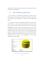
3D MODELING AND DESIGN ------------------------------------------------------------------------ 52
ADDITIVE MANUFACTURING OR 3D PRINTING ----------------------------------------------- 58
ASSEMBLY ----------------------------------------------------------------------------------------------- 61
CHAPTER 4 --------------------------------------------------------------------------------------------------------- 63
4.1.
CONTINUOUS ROTATION MODIFICATION ----------------------------------------------------- 65
CHAPTER 5 --------------------------------------------------------------------------------------------------------- 69
5.1.
5.2.
5.3.
5.4.
MICROCONTROLLER--------------------------------------------------------------------------------- 70
MICROCONTROLLER PROGRAMMING ---------------------------------------------------------- 74
WI-FI MODULE ---------------------------------------------------------------------------------------- 81
WI-FI MODULE PROGRAMMING ------------------------------------------------------------------ 90
CHAPTER 6 -------------------------------------------------------------------------------------------------------- 101
6.1.
JAVA GUI ---------------------------------------------------------------------------------------------- 103
6.2.
ANDROID DEVELOPING PLATFORM ------------------------------------------------------------- 106
6.3.
BASICS OF APPS DEVELOPMENT ------------------------------------------------------------------ 108
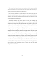
6.4.
APPLICATION FOR ROBOT CONTROL ----------------------------------------------------------- 115
6.4.1.
Main activity -------------------------------------------------------------------------------- 116
6.4.2.
Control activity ---------------------------------------------------------------------------- 118
CHAPTER 7 -------------------------------------------------------------------------------------------------------- 125
xi
REFERENCES ----------------------------------------------------------------------------------------------------- 129
APPENDICES ------------------------------------------------------------------------------------------------------ 133
xii
List of figures
Figure 1: Robot Devastation logo
Figure 2: Robot Devastation PC interface [1]
Figure 3: This project's Android controlled robot
Figure 4: Project’s workflow: Design, hardware and smartphone programming.
Figure 5: CNC machine
Figure 6: CAD/ CAM systems
Figure 7: CATIA design and rendering
Figure 8: Professional and domestic use 3D printer
Figure 9: Intel 4004, the first commercial microprocessor
Figure 10: Basic Von Neumann processor architecture
Figure 11: Die of an 8-bit PIC EEPROM microcontroller by Microchip [21]
Figure 12: Some common microcontroller applications
Figure 13: Arduino UNO: The most used Arduino microcontroller
Figure 14: Raspberry Pi
Figure 15: Tiny AVR ISP programmer [25].
Figure 16: LiPo battery and small-sized solar cells [26]
Figure 17: VIew of the Arduino development environment [24]
Figure 18: Two-pole brushed DC motor
Figure 19: Floppy-Disk brushless DC motors
Figure 20: Industrial servomotor
Figure 21: Servo block diagram
Figure 22: Common servo parts
Figure 23: Power consumption of different locomotion mechanisms [33]
Figure 24: (a) Wheeled robot; (b) Kovan robot & (c) NASA’s wheeled robot.
Figure 25: Smartphone share per region
Figure 26: US smartphone penetration
Figure 27: Software and hardware platform pie
Figure 28: Apps available per platform
Figure 29: Platform market development
Figure 30: A look into the OpenSCAD software [8]
Figure 31: View of the LiPo battery
Figure 32: 3D representation of a TowerPro sg90
Figure 33: 3D view of the Arduino Fio board with the RN-XV on it
Figure 34: View of the front part
Figure 35: 3D model of the rear part plug
Figure 36: Rear part support
Figure 37: Top view of a wheel
Figure 38: Unassembled complete robot
Figure 39: OpenSCAD to STL format and STL to G-Code [40]
Figure 40: A view of the software Replicator G [40]
Figure 41: 3D printer building a wheel. [40]
Figure 42: Preassembled robot
xiii
2
3
6
8
13
13
14
15
18
19
24
25
26
28
29
30
31
36
37
38
39
40
42
44
46
47
47
48
49
52
53
54
54
55
55
56
56
57
59
59
60
61
Figure 43: Assembled complete robot
Figure 44: Top view of the assembled robot
Figures 45, 46 [41], 47, 48 & 49: Unscrewed and modified servo
Figure 50: Potentiometer's wires [42]
Figure 51: Tin ends [42]
Figure 52: Soldered resistors [42]
Figure 53: Arduino FIO
Figure 54: ATmega328P [16]
Figure 55: Main Arduino block diagram
Figure 56: Block diagram for storing string and converting to integer
Figure 57: Robot, servos and battery layout
Figure 58: Roving-Networks RN-XV 171 Wi-Fi module [29]
Figure 59: Wi-Fi module operating modes [44]
Figure 60: Typical TCP applications [44]
Figure 61: FTP client/ server configuration [44]
Figure 62: HTML client configuration [44]
Figure 63: GPIO_9 to VCC & Figure 64: Module powered by FIO
Figure 65: Wire for short-circuiting GPIO_9 to VCCC.
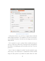
Figure 66: Wireless connection configuration
Figure 67: Layout for serial communication
Figure 68: Telnet communication between Laptop and Wi-Fi module
Figure 69: Console commands for running Java
Figure 70: Java User interface program for robot control
Figure 71: Client-server connection: client request [49]
Figure 72: Client-server connection: server accepts connection [49]
Figure 73: Android SDK manager [50]
Figure 74: Basic steps for apps development [50]
Figure 75: AVD Manager [50]
Figure 76: Project phases [50]
Figure 77: Activity lifecycle [50]
Figure 78: Main activity and Control activity
Figure 79: Main activity’s graphical layout
Figure 80: Block diagram for the Main activity
Figure 81: Graphical layout for the Control activity
Figure 82: Control Activity block diagram
Figure 83: Second thread's block diagram
Figure 84: Multi-threading behavior
Figure 85: Concept of Robot Devastation by Santiago Morante
xiv
62
62
65
66
66
66
71
71
76
77
80
81
83
85
86
86
91
91
93
96
97
103
104
104
105
107
108
110
111
113
115
116
117
118
121
122
124
127
List of tables
Table 1: Basic information about CPU architectures [14]
Table 2: CISC vs RISC CPU architectures
Table 3: Widely used servos and their features [28]
Table 4: Arduino FIO features
Table 5: Set commands parameters
Table 6: Default access point mode settings
xv
20
21
41
72
84
87
xvi
Chapter 1
Introduction
Nowadays, a new way of interacting
with robots is starting to develop
among both professionals and nonprofessional electronics users. Due to
the recent development of open
source software and more recently
open source hardware, as well as the
decreasing prices in the world of
electronic tools, engineers find themselves in a situation where they can
think of and carry out a vast range of projects. These projects may start
out of the industrial environment per se, however, most of the
experience, technical abilities and new ideas are subject to be applied
later on in the industry of robotics.
There is, consequently, an approach between consumer electronics and
traditional electronic components for developers, motivated by the
philosophy of open tools, affordable for all users, which let engineers
incorporate a wide range of functionalities to their projects.
1
Considering these open tools as framework, a big project is being
developed at this time combining innovative ideas, wireless technologies
and an open philosophy for users to become an active part of the big
system. This idea is called ‘Robot Devastation’, a new-generation shooter
with augmented reality and real robots. Users will be able to play online
with others with a smartphone or PC, moving robots in championships
and campaigns. Everything 24/7.
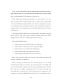
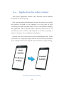
Robot Devastation (Fig. 1) is the big final project that serves as
framework for ASROB, the UC3M Student Robotics Society, to develop a
variety of projects related to it. If we talk about the future of Robot
Devastation, this project has opened the way to the upcoming
developments in each field related to it, as it is only in an embryonic stage
and there is always much to create and improve.
Figure 1: Robot Devastation logo
The idea: Users’ robots will be located in the same place and they will
be equipped with a locomotive system and a camera as the minimum
gear. These robots would be printable and open-source, although this
could not be a requirement, and be adjusted to a series of parameters to
be considered “legal” to enter this system.
Users could be located at any place in the world as long as they have
access to the network, and would be able to control their robots either
with a PC or their smartphone (preferred option to gain portability).
2
Last but not least, there will be a server in charge of managing all field
data, that is to say, anything relevant that happened at the location where
these robots would interact. In order to talk in greater detail about the
server’s behavior we should first define what kind of interaction there is
supposed to be among the robots.
The purpose of this idea is to create a competitive environment
modeled as a shooter game (classic first person shooting games) where
users will compete and battle against others at anytime from anywhere.
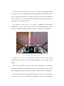
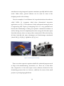
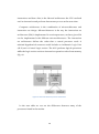
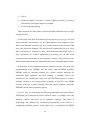
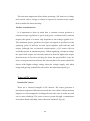
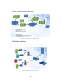
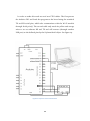
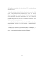
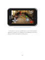
Figure 2: Robot Devastation PC interface [1]
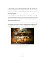
In figure 2, we can see a prototype interface (for PC) with virtual
shooting lasers to give users the right perspective of the target (other
robot).
The server will keep record of all events happening in real time,
receiving information about which robot is shooting which one, where
this is happening, when, and also information about points, rankings, etc.
This facet of the Robot-Devastation project has not been covered at all
in this project as it is in the field of computers science programming,
3
more suitable for computer science students, hence being an ambitious
project with modules in different areas of expertise. However, in this
project in particular, a mobile robot has been built thought to be suitable
with Robot Devastation as a first approach to the initial idea.
In addition, according to the philosophy of the robotics association,
almost all material used in this project is open-source, both hardware and
software, and the developments achieved in every area are constantly
being published so that others can use what they consider is useful for
their own projects. This assures that with a low-budget, we can develop
applications that meet most of the requirements.
4
1.1.
Motivation and aim of the project
Among all the technological and conceptual challenges faced in this
project, there is one above all, which is meant to serve as a breaking point
in the world of common user robotics, amateurs, and engineers, and this
is enabling a certain mobile robot to be controlled from a smartphone
using no more than an internet connection.
Given that the great majority of users have access to smartphones, an
option to give wireless connectivity for any purpose comes handy so that
developers will not concern themselves about implementing new
hardware and software options to their existing projects. Instead, they can
adapt their projects to be compatible with current connectivity protocols
such as Wi-Fi or Bluetooth, and use a phone to interact with them. This
means that any of them would be capable of controlling their hardware
from their phones contrary to having to develop any significant extra
parts.
Given this, we could make use of smartphones to our benefit with the
purpose and idea of Robot Devastation. As it is in an Alfa state, there was
no tangible ‘product’ related to Robot Devastation around which we could
start to develop the applications and dynamic systems derived from it.
Hence, the need to create a small mobile robot capable of being
controlled from Android platforms making use of the most suitable
wireless technologies available, which are for now, Wi-Fi internet
protocols.
If we want users to be able to create their own robot designs as well as
building them using layouts available on the internet we should make use
of open hardware manufacturing tools such as the recent 3D printers,
which are increasing their presence in many environments.
5
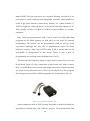
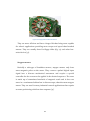
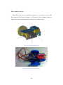
According to this open philosophy and as a need to materialize the
user-client part of Robot Devastation, a concept of a robot is born for this
project. It should be ready to connect to a wireless network almost
instantly upon power on and subject to being controlled from a user
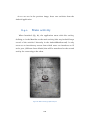
interface with no delay in the communications. In addition, it should be
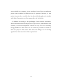
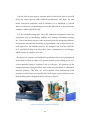
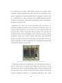
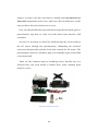
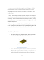
printable as mentioned before. All this requirements have been met in the
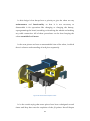
robot built for this project; figure 3.
Figure 3: This project's Android controlled robot
Apart from achieving the communications part (wireless internet data
transfer, low latency and reaching long distances between the operator
and the robot), another important objective is to develop the robot and
its associated communications system under a low-cost and open source
philosophy (always if possible, depending on the part). This way we can
bring potential future users closer to the project since the whole robot
costs less than $100 (see Appendices).
The third objective/ challenge would be to provide the robot with a
high autonomy in the sense of hours of use without the need for
recharging. At the moment, the robot uses a LiPo battery which is a long
battery life, but it could be enhanced by using solar cells (future versions,
see Chapter 7, conclusions and future work).
6
1.2.
Parts of the project
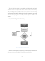
The first part is the design, manufacture and assembly of the robot’s
structure. For the purpose of 3D designing, a parametrical modeling
software was used which will be discussed later along with other
discarded options. Regarding the manufacture, the code from the 3D
software is then translated into a machine code that can be read by a 3D
printer which builds each piece layer by layer. Once the pieces are
complete, they are assembled including the electronic components and
the robot reaches its final shape, and we then proceed to modify the
servos to achieve continuous rotation by hacking the electronics as well
as its mechanical structure.
This is all covered in Chapter 3 (3D) and Chapter 4 (servos).
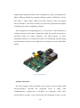
The second part concerns the programming and configuring the
electronic components for this project. First the microcontroller board
called Arduino based on the ATmega328P running at 8 MHz serving as
the main “intelligence” for the robot. This board is in charge of reading
the wireless transferred data and moving the robot’s DC motors. Second,
there is a smaller Wi-Fi module thought to be plugged on the Arduino
enabling wireless connectivity with any device with internet connection,
such as laptops, smartphones or other Wi-Fi boards. The main board is an
open source electronics platform, which users can build from common
single electronic components or buy preassembled. The programming
software can be downloaded for free. The Wi-Fi board, is not open source
hardware, but can be configured following its user’s manual.
This is all covered in Chapter 5.
7
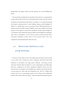
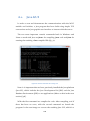
The third and last major part covers all the Java programming first for
a Laptop and then for a smartphone, including socket processing, user
graphics interface and data calculations, all destined to the creation of an
intuitive application for moving the robot that is both simple and robust.
This is all covered in Chapter 6.
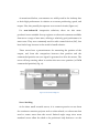
Figure 4: Project’s workflow: Design, hardware and smartphone programming.
8
1.3.
Document structure
Having passed the introductory part of this document (section 1), in the
next chapters of the text we are going to discuss more extensively the
different parts of the development of this project.
In the second section, we review the background technologies and
environment surrounding every major part of this project.
In the third section, the design, manufactory and assembly of the
pieces involved in the robot are going to be exposed in detail, as well as
the procedures and tools involved.
In the next and fourth chapter we proceed to describe the election,
electronic modification and implementation of the servos used as DC
motors that make the robot’s movement possible.
In the fifth chapter, we will take a look at the electronic configuration
and hardware choice as well as all the programming.
Next, in the sixth section, we will discuss all topics related to the
smartphone remote controlling and programming involved.
In the last section, we can find the conclusions to this project.
9
10
Chapter 2
Background
In the context of robotics there
is much to be discussed about
the technological challenges
and
possible
implementations
different
for
each
single project or solution as a
result
of
the
increasing
development and progress in every area involved. New ideas lead to new
projects and every one of these projects lead to new ideas for improved
projects, often as an exchange of resources between different parties. This
interaction between developers among the world translates into an
accelerated progress, in which anyone, from companies to single
engineers can take part.
This technological background and its influences are discussed in this
part of the report, dividing it the same way as the main document is
structured. First, we talk about the background of 3D modeling and
designing, followed by the background of electronics hardware and
programming. Third, we will take a look at the implementation and
incorporation of electric actuators and DC motors usually found both in
industrial environments and in other electronics projects. Fourth and last,
11
we discuss the foundations and background of smartphone oriented
programming.
In all parts we start from a generalist point of view, talking about
possible different implementations, and then converge around the
particular cases involving this project.
2.1.
Mechanical Structure
In order to build a machine’s structure there are many professional and
non-professional solutions in the market. For the most demanding robots
the industry provides manufacturing methods and solutions that suit
high precision requirements, high torques and forces, and machine parts
that withstand high stresses and have a stable response during time. This
is the case, for example, of robots used in assembly lines or paint shops.
As the execution and field performance of these industrial robots must be
robust and precise they are manufactured with the best suitable
composite materials, such as carbon steel, titanium compounds or carbon
fiber. Cast iron, steel and aluminum are most used for arms and bases.
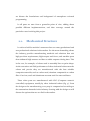
These robot parts are manufactured with CNC (Computer numeric
controlled) equipment, usually by other industrial robots (fig. 5). From
the design to the manufacturing, every step is computerized according to
the automation demands in the industry. Starting with the design we will
discuss the options that we can find in the market.
12
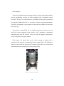
Figure 5: CNC machine
If we focus entirely on the engineering side of designing leaving on a
secondary level the artistic approach we come across several software
options where we can find what best suits our projects’ needs, although it
is never really possible to separate these two sides of designing. The two
main concerns that arise when having to choose a certain program are
budget and the complexity required. We will take a look at this more
deeply further in this part.
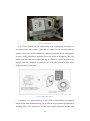
Figure 6: CAD/ CAM systems
In practice, it is most common to use CAD/ CAM solutions (computer
aided design and manufacturing, fig. 6) which are programs specialized in
working with CNC machines. In the same plant engineers design and
13
manufacture using integrated systems sometimes specially built for their
needs. Other times, general software can be used for most of the
designing needs in the industry.
First, for example, it is well known for its professional use the software
called CATIA [2] (computer aided three dimensional interactive
application, see fig. 7). This software is fairly widespread among all areas
of engineering that require 3D designing and it is a very powerful tool,
but has the disadvantage of being an expensive commercial software as
well as having a level of complexity above the average for this task. Apart
from this software, there are many other commercial CAD tools, but they
all share basically the same advantages and disadvantages mentioned
(AutoCAD [3], AC3D [4], LightWave 3D [5], etc.)
Figure 7: CATIA design and rendering
These are rather expensive options suitable for industrial purposes such
as large scale manufacturing, aeronautics, etc. There are, on the other
side, inexpensive or free tools (open source software) destined for less
demanding projects that are, however, sufficient for most of the small
projects or prototyping applications.
14
On the side of open source software tools we have less choice, but still
there are some options with different peculiarities. We have, on one
hand, interactive modelers such as Blender [6] or MeshLab [7] which
allow for advanced 3D modeling, and on the other hand, a 3D parametric
compiler called OpenSCAD [8].
For the manufacturing part, the CNC industrial equipment carry out
operations such as machining, milling, laser cutting, threading, turning,
etc. These machines execute code extracted from the designing software
and execute movements according to a generated a set of instructions for
each operation. For smaller projects, the designer can send the CAD file
to a specialized shop and have their piece manufactured accordingly,
which results in a higher unit cost.
Recently it is common to find both in professional and non-professional
environments what is called a 3D printer which works adding layers of a
certain material using a machine code as reference. 3D printers can be
categorized from high precision state-of-the-art machines to affordable
amateur printers. The first, are used together with professional CAD
systems and the latter are usually used with open source software tools,
both working with a digital model as reference (fig. 8).
Figure 8: Professional and domestic use 3D printer
15
The pieces modeled with CAD software have to be “sliced” in order for
the printer to be able to build each layer. With the CAD software, in this
case OpenSCAD, we export the components into a STL format [9] which
is an intermediate data interface between the rendering software and the
machines code. This STL format approximates the object using triangular
facets which, the smaller they are, produce a higher quality of surface.
3D printers have a working process called additive manufacturing since
it works by adding successive layers of a special polymer until it “prints”
the whole piece. Additive manufacturing is opposed to the traditional
subtractive manufacturing which is a retronym for standard machining
operations that use a raw object (filling, turning, milling, etc.) One
advantage worth mentioning is that this technique allows for almost any
shape, excluding thin based pieces that cannot support their own top
parts.
A typical layer thickness resolution for 3d printers is 0.1 mm, although
there are models such as the 3d systems’ ProJet series [10] that allow for
lower resolutions, up to 16 micrometers. In the industry it is common to
print a slightly oversized version of the object and then use a higher
resolution subtracting process to remove the remaining material.
One last and important advantage of 3d printers is that most of them
are approximately desktop sized, and certainly smaller than the common
subtractive machines. This is the reason why it is advantageous to first
print the piece and then perform machining processes on it.
Various polymers are used in 3D printers such as acrylonitrile
butadiene
styrene
(ABS),
PLA
(ecological),
polycarbonate
(PC),
polyphenylsulfone (PPSU) and high density polyethylene (HDPE). These
polymers come as a filament wrapped around a cylinder forming a coil.
This filament goes into the extruder and when it reaches the adequate
16
temperature the plastic melts and the printer can start building the
layers.
The previously mentioned non-professional printers are progressively
entering the world of DIY (do-it-yourself) projects both in private and in
academics environments (Universities, toy-shops). It is worth mentioning
the longest running project in the desktop category called RepRap [11]
which is a totally open source 3D printer whose full specifications are
released under the GNU General Public License and capable of printing
many of its own parts to create more machines. Another good example of
a 3D printer is the Airwolf 3D (Prusa) which is also widespread among the
open source community. In 2011 and 2012, prices of these printers have
decreased drastically as they used to cost around 20000 US $ [12]
compared to the less than $1000 that cost now.
2.2.
Electronic hardware and
programming
Previous to the release of the first single-chip microprocessor by Intel
in 1971, there were, during the 1960s, computer processors built with
hundreds of transistors and logic gates soldered, connecting several
electronic boards which resulted in a poor performing and substantial
heat loss, compared to the later integrated solutions. These were the
boards used, for example, in the Apollo space mission [13] during the late
60s and early 70s. After this, the integration of a CPU in a single chip
reduced the cost of processing power and its large scale production
system led to lower unit costs (fig. 9). This automated manufacturing also
17
led to doubling the number of components that could fit in a chip every
two years [14]. These single chips had fewer electrical connections and
thus an increased reliability. The world of electronics was soon to be
revolutionized.
Figure 9: Intel 4004, the first commercial microprocessor
The previous medium-scaled integrated circuits architecture was used
in the first microprocessors. The first, were used in calculators and other
embedded systems such as terminals or automation devices. After this, in
the mid-70s, they appeared in the first microcomputers. From this
moment on, microprocessor architecture design starts to develop and
expand.
In 1945, John Von Neumann published his organization of logical
elements which IBM used to develop the IBM 701, the company’s first
commercial stored-program computer in 1952. Opposed to the Von
Neumann architecture in which there are shared signals and memory for
code and data, and the CPU can be either reading an instruction or
writing/ reading data to/ from the memory, we have the Harvard
architecture with physically separate storage and pathways for
18
instructions and data. Also, in the Harvard architecture the CPU can both
read an instruction and perform data memory access at the same time.
Computer architecture is the combination of microarchitecture and
instruction set design. Microarchitecture is the way the instruction set
architecture (ISA) is implemented in a microprocessor, so that a given ISA
can be implemented with different microarchitectures. The instruction
set architecture defines the codes that a central processor reads. A
minimal hypothetical structure would include an Arithmetic Logic Unit
(ALU) and a Control Logic section. The ALU performs logical operations
while the logic section retrieves instruction operation codes from memory
(fig. 10).
Figure 10: Basic Von Neumann processor architecture
In the next table we can see the differences between many of the
processors found in the market.
19
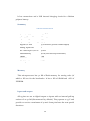
Table 1: Basic information about CPU architectures [15]
Architecture
Bits
Alpha
64
ARM
32
ARM
64
AVR32
Blackfin
DLX
32
eSi-RISC
Itanium (IA64)
M32R
m68k
RISC
32
No
RISC
16
Unknown
RISC
30
Unknown
RISC
15
Unknown
8
Unknown
Unknown
32
1990
RISC
32
RISC
ago-72
No
EPIC
128
Yes
1997
RISC
16
Unknown
1979
CISC
16
Unknown
32
64(32→6
4)
64
PARISC (HP/PA)
64(32→6
PowerPC
32/64(3
S+core
16/32
4)
2→64)
Register2009
Register
Register2001
Register
RegisterRegister
Register1981
Register
Register1999
Register
2006
1986
1991
32
1982
64(32→6
1985
4)
32 1990s
1964
VAX
32
1977
x86
32(16→3
1978
2)
64
RegisterRegister
2005
System/360 /
(32→6
System/370 /z 64
4)
/Architecture
x86-64
Open
RISC[4]
16/32
SuperH (SH)
Registers
2000
32
Series 32000
Design
32
64
MMIX
SPARC
Type
Register1992
Register
Register1983
Register
Register2011[2]
Register
2006
16/32
Mico32
MIPS
Introduced
2003
RISC
32[6]
Yes[7]
RISC
32
Unknown
RISC
256
Yes
RISC
32
No
RISC
32
Yes[9]
RISC
MemoryMemory
RegisterRegister
RegisterRegister/
RegisterMemory
RegisterMemory/M
emoryMemory
MemoryMemory
RegisterMemory
RegisterMemory
20
Unknown
CISC
RISC
8
31 (of at
least 55)
Unknown
Yes
RISC
16
Unknown
CISC
16
Unknown
CISC
16
Unknown
CISC
8
No
CISC
16
No
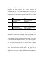
Today, most CPU architectures implement one of the next two
instruction set design strategies: RISC,
reduced instruction set
computing, that uses a small, highly-optimized set of instructions that
provide a high performance and a fast execution as opposed to CISC,
complex instruction set computing with a specialized and more complex
set of instructions.
1
2
3
4
5
6
CISC
Emphasis on hardware
RISC
Emphasis on software
Multi-clock complex
instructions
Small code sizes
Single-clock, reduced
instructions
Larger code sizes
Many addressing modes
Easy compiler design
Pipelining does not function
correctly because of
complexity of instructions
Few addressing modes
Complex compiler design
Pipelining not a major
problem, this option speeds
up the processors
Table 2: CISC vs RISC CPU architectures
In table 1, we can observe the famous Intel’s x86, which is a family of
instruction set architectures, based on the 8086 (1978). Another worth
mentioning microprocessors are the AVR [16] and ARM [17] families.
Intel has been one of the most important players in the recent history
of microprocessor and embedded systems. As seen in the first picture of
this chapter, the 4004 was the first commercial microprocessor by Intel in
1971. This 4-bit microprocessor was soon followed by an 8-bit 8008
processor, the first of its kind, which in turn was followed by the very
successful 8080 (1974) with a much improved performance, being the first
widely used microprocessor. Motorola had, at the same time, its
competitor 6800. Later on, in 1978, a 16-bit processor called the 8086 was
released and it was the first of the x86 family which powers most modern
PC type computers. In the early 80s we started to see the first 32-bit
21
processors being one of the most important the Motorola MC68000 [18].
Along with this processor another 32-bit worth mentioning units are the
AT&T BELLMAC 32-A (the first with 32-bit data paths, buses and
addresses), Intel’s iAPX 432 and the first ARM (1985).
The next step were the 64-bit processors, which we could find in the
90s in several machines such as the Nintendo 64 gaming console,
however, it was not until the early 2000s that this microprocessors
targeted the PC market. Today the PC market is majorly divided between
AMD and Intel, with an important share for both 32-bit and 64-bit
architectures.
Microcontrollers
Sometimes abbreviated µC or MCU, microcontrollers are integrated
circuits that can act as small computers used for embedded automatic
controlled products or devices. Microcontrollers contain a similar
structure as found in regular computers, integrating in a single circuit a
processor core, memory and programmable input and output peripherals.
The core is a microprocessor as described before, but there are several
features that make microcontrollers the preferred solution for most
systems that require an automatic response and behavior.
The following parts are usually found in a microcontroller:

Central processing unit (CPU), ranging from 4 up to 64 bits.

Volatile memory (RAM) for volatile data storage.

Non-volatile program memory. This can be PROM, EPROM,
EEPROM or flash.

Serial input and output such as serial ports, and other serial
communications interfaces (SPI, I2C, etc.)

Peripherals such as timers or PWM generators.
22

Clock

Analog-to-digital converter or/and Digital-to-analog converter,
with analog and digital inputs or outputs.

In-circuit programming.
These features are what make a microcontroller different from a single
microprocessor.
At the same time that Intel started producing the 4004 (1971), the first
microcontroller was about to see the light thanks to the engineers Gary
Boone and Michael Cochran [19]. The result of their work was the TMS
1000, the first lone-chipped CPU which went commercial in 1974. Soon
after, and partly in response to this, Intel developed the 8048 (1977), a
chip optimized for control applications becoming one of the most
successful microcontrollers in the company’s history. They sold over one
billion 8048 chips mostly for keyboards and other numerous applications.
At this time, microcontrollers had two memory variants. One was only
programmable once (PROM) and the other, called EPROM (erasable
PROM) could be rewritten thanks to a quartz window allowing for
ultraviolet light exposure and thus making it erasable. These two
memories were actually the same, but the EPROM required a ceramic
package instead of an opaque plastic package as found in the PROM
version. Only the ceramic package with the quartz window made the
EPROM a much more expensive option.
Later, in 1993, an electrically erasable programmable read-only memory
(EEPROM) was introduced which allowed users to quickly erase the
memory without the need of an expensive package. This kind of
technology also allowed for in-system programming (write data in a
completely installed system). In the same year, a new kind of EEPROM
23
was introduced by Atmel called Flash memory and quickly other
companies started manufacturing with this kind of technology. In the
future, a possible new technology still under development could be used
as a replacement for flash memories: The MRAM (magnetoresistive
random-access memory), with a better performance, power consumption,
and faster access times [20].
Nowadays, the unit cost of microcontrollers has decreased to a
minimum, resulting sometimes, in $1 or fractions of a dollar per unit. It is
estimated that around 55% of all CPUs are 8-bit microcontrollers of
microprocessors. These inexpensive 8-bit processors suit perfectly for
endless purposes such as automobiles, office and home systems, medical
equipment, robots, toys, remote controls and many other embedded
systems. 8-bit processors have the advantages of being robust and easy to
program and they are rather inexpensive low consumption solutions with
a size that fits almost in any system.
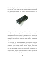
Figure 11: Die of an 8-bit PIC EEPROM microcontroller by Microchip [21]
Depending on the system requirements we can find processors from 4bits, for devices that can operate with small data sizes, up to 64-bits
microprocessors for the most demanding systems. The first, together with
8-bit processors can be found in digital calculators (HP-48) and remote
controls, although nowadays it is becoming difficult to find 4-bits
24
processors. 8-bit processors enable engineers to support a wide range of
applications and functions including automotive, motor control, LCD
drivers, USB connectivity, lighting applications and more. A typical midrange automobile is estimated to have around 30 microcontrollers,
typically for window lift, low end airbags, pumps, steering angle sensors,
cooling fans and valve/ throttle control. This is the case, for example, of
the 8-bit microcontroller family XC800 by Infineon [22]. However, in
both industrial and automotive applications, it is becoming more
common to find 32-bit microcontrollers as its unit cost is similar to the
previously mentioned processors, but these can operate with bigger data
sizes (fig 12.).
Figure 12: Some common microcontroller applications
It is worth mentioning a family of modified Harvard architecture
microcontrollers from Microchip Technology called PIC [23], (Peripheral
Interface Controller, see figure 11) popular among both industrial
developers and hobbyists due to low cost and wide availability (users
could usually get free samples). Also used for educational purposes, these
microcontrollers have been used in the last years and have become
tremendously famous.
In the last few years, supported by the internet community, there has
been a substantial growth in the use of a new kind of open source
microcontrollers and programmable hardware by a new generation of
enthusiasts all around the world that use them as powerful tools to carry
25
out projects either in the field of education or just as a hobby. For
engineering students or graduates these new microcontrollers serve as
great tools for developing their ideas or projects. Where PIC
microcontrollers used to be the rule for small projects, prototypes and
hobbyists devices a new family of microcontrollers called ARDUINO [24]
has displaced it, becoming, in short time, a very famous tool for
developing
almost
any
engineering
project
that
requires
a
microcontroller.
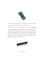
In 2006, the Arduino Uno was announced (Fig. 13), and from then on,
the Arduino community started. This project is based on an Arduino
microcontroller,
and
therefore,
we
will
explore
in
detail
the
characteristics of this product.
It is quite essential, nowadays, that for a kind of technology such as this
to succeed there is a huge community behind it to support it as well as a
vast source of information where developers can easily find the solution
to their problems and at the same time contribute to that community to
help others.
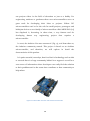
Figure 13: Arduino UNO: The most used Arduino microcontroller
26
As we can see in the picture, in the Arduino microcontrollers we have a
typical layout where we can easily spot the microprocessor, input/ output
pins, serial peripherals, USB connector, a button, etc.
What makes this technology preferable over other options is the fact
that every part of the Arduino family devices is open source, what makes
it more accessible and maintainable. From users to companies everyone
can contribute either writing new software such as libraries, firmware or
program codes or developing new electronic boards based on the Arduino
configuration.
The original Arduino boards are manufactured by the Italian company
Smart Projects, and other typical Arduino-branded boards have been
designed by the American company SparkFun Electronics.
Some of the official boards:

Arduino Extreme with USB interface and ATmega8.

Arduino Mini, a miniature version using ATmega168.

Arduino Nano, even smaller with ATmega328.

Arduino Bluetooth, with a Bluetooth interface.

Arduino Mega with additional I/O and memory.
Many other Arduino boards can be found in the market manufactured
by other companies or engineers.
Before starting in detail with the Arduino project, it is worth
mentioning that other new devices are just starting to see the light and
seem to be plausible competitors for the most demanding needs. Projects
that may need a higher computing power and more versatility are
becoming more frequent since they incorporate all components of a
computer in a single embedded electronic board. As an example, we have
27
single-board-computers (SBC) such as Raspberry Pi (fig. 14, BeagleBoardXM or iMX233 suitable for running desktop software (Windows, Linux)
and with a much larger RAM and flash memory than the typical
microcontrollers. Processors on SBCs are also more powerful and capable
of dealing with more computing workload.
This integration of computing power is an answer to the demands of
complex systems of processes. Optimized chips for specific processes or
particular tasks are rather expensive and rigid options, so these
embedded systems are usually the answer for integrating all processing
and automation power in one single board, resulting in a more affordable
option.
Figure 14: Raspberry Pi
Arduino Hardware
The first Arduino microcontrollers were based on 8-bit Atmel AVR
microcontrollers,
typically
the
megaAVR
series
of
chips,
with
complementary components to facilitate its integration with other
circuits. More recently, a new version has been designed around a 32-bit
28
Atmel ARM. The pin connectors are exposed allowing the board to be
connected to other external interchangeable modules called shields in
order to get extra features (connectivity, battery, etc.). Most include a 5
Volt line regulator, although there can be found some that operate at 3V.
They usually include a 16 MHz or 8 MHz crystal oscillator or ceramic
resonator.
They come pre-programmed with a boot loader to help uploading
programs to the flash memory so that they do not need an external
programmer. All boards can be programmed with an RS-232 serial
connection although the way this is implemented varies for some
hardware versions. They use an FTDI cable (USB to serial) that can be
detachable or incorporated to the board. There is also a way of
programming it wirelessly either by Bluetooth or Wi-Fi.
The fact that the hardware design is open source means that users can
be perfectly aware of every component of the board and, what is more,
they can build their own version with single electronic components that
are found in any electronics store. This way, developers can also program
the microprocessor with an AVR programmer for the firmware (Fig. 15).
Figure 15: Tiny AVR ISP programmer [25].
Some companies such as DIGI, Roving-Networks or Adafruit Industries
manufacture shields that suit Arduino projects. Roving-Networks and
29
DIGI have a variety of Radio modules that can operate with Bluetooth or
Wi-Fi protocols and Adafruit makes, for example, a special shield for
motor control.
Arduino boards can be powered with normal 9V or 5V batteries, LiPo
batteries and also have a solar panel support (Fig. 16).
Figure 16: LiPo battery and small-sized solar cells [26]
Arduino Software
In order to program the Arduino microcontrollers, the founders of the
project designed and created a tool intended to be easy and intuitive for
new users. This is called the Arduino IDE (integrated development
environment), a Java written program that allows developers to write,
debug and compile programs as well as uploading them to the electronic
board. It is derived from the Processing [27] programming language IDE
which is an open source programming language built with the purpose of
teaching the fundamentals of computer programming in a visual context.
The programs written for the Arduino are called Sketches and are
written in C or C++. The IDE comes integrated with some libraries such as
the Wiring library which makes it easy to operate with inputs and
outputs, and other standard libraries for working with extra hardware
30
(servos, internet shields, steppers or LCDs). Nevertheless, Developers can
include extra libraries either creating them for particular needs (extra
hardware, specific math functions, etc.) or using other developers’
libraries. In line with the philosophy of open source coding, developers
usually publish their new libraries and maintain the code for others to
incorporate them in their own projects. These projects, if published, at
the same time serve as guidance and support for others. This cyclic
contact is what nourishes the developer’s community, and in the end
contributes to the Arduino project. In fact, as soon as a new piece of
hardware that is subject to be incorporated to Arduino boards goes
commercial, documentation in the form of libraries, code examples and
troubleshooting instantly appears on specialized Arduino and DIY
forums.
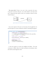
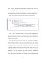
In order for users to make runnable cyclic executive programs in
Arduino, they only need to write two functions called setup() and loop().
The First, is executed only once for initializing settings and variables. The
loop() function runs cyclically until the board powers off (fig. 17).
Figure 17: VIew of the Arduino development environment [24]
31
All Arduino software tools are available for Windows, Linux and Mac
platforms.
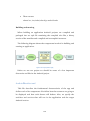
Communications hardware
As mentioned before, Arduino boards allow for external modules or
shields to be attached to them in order to provide extra features to an
existing design. In particular, for external communications we have
devices either for wired or wireless connections. For the first, there is for
example, an Ethernet shield capable of providing internet (RJ-45)
connections, and for the latter we can choose among various technologies
depending on the protocols they use.
There are plenty RF modules available in the market belonging to the
WPAN standards (wireless personal area networks) that operate in the
802.15 frequencies working group. The IEEE 802.15 is a group of standards
for local area communications used in many devices and products. For
example, we have the DIGI’s ZigBee RF modules [28] that use the 802.15.4
standard or other DIGI’s modules with 802.15.1 (first Bluetooth assigned
standard). Apart from Bluetooth, and radio frequency, makers such as
Roving-Networks or DIGI among others sell 802.11 b/g/n modules for WiFi connections, capable of acting as server or clients depending on the
desired topology or our system.
From all available devices for wireless communications, we have to
choose one that is suitable for Arduino, not very expensive and pluggable
into an XBee socket. At this point we have two options, first a DIGI’s XBee
Bluetooth module, which in short acts as a node for an Ad-Hoc
connection allowing for two XBees modules to interact in short distances
with low power consumption. Second, we have the option to use a Wi-Fi
32
module (Roving Networks RN-171 [29]) which is a little bit more
expensive.
The first module is easy to configure on windows, with a program
called X-CTU but users need an extra device for it, an USB adapter. Also,
these modules are thought to be used normally in pairs, communicating
with one another so it is a bit of an issue to get one working with a more
complex device, for example a smartphone. Another disadvantage of the
Bluetooth module is that it only works well in short distances allowing
only for Ad-Hoc connections. On the other hand it has three worth
mentioning advantages which are lower consumption than the Wi-Fi
module, lower market price and is easier to use.
The second option is the RN-171 Wi-Fi module which allows for more
complex types of wireless networks. Users can interact with this module
in Ad-hoc mode and more importantly, with an access point. Both ways
this module can act as a server or as a client depending on what role it is
playing in a specific topology. A drawback for using Wi-Fi Ad-hoc
connections with Android is that only the last version (4, Jelly Bean)
allows for it.
33
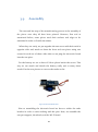
2.3.
DC Motors
In the world of robotics, most of the times engineers incorporate DC
motors to every kind of robot due to the electronic controlling
advantages, motor sizes and the fact that robots are usually powered by
DC currents and voltages. In the industry, robot actuators can also be
pneumatic or hydraulic differing only in their capability to pressure the
fluid. Pneumatic actuators, compared to hydraulic, are low cost ecological
solutions for less demanding forces whereas hydraulic actuators stand
high power loads. Both have the advantage of having non-electrical
components, making them the best option for critical environments or
processes.
The third and previously mentioned option, the electric actuators, is by
far, the most implemented in industrial or domestic robots. There are
basically three kinds of electric motors: AC, DC and stepper motors. In
high-power single or multiphase industrial applications AC motors are
used where a constant rotational torque and speed is required to control
large loads. On the other hand, for light duty applications and since many
autonomous robots are powered by DC batteries, the actuators that they
incorporate must be DC motors or steppers. These are used along with
microcontrollers, positional electronics and small robots.
Before entering into the types of DC motors we will discuss some
important variables that should be considered when designing robot
motion functionalities.
34
The two most important values when powering a DC motor are voltage
and current, where voltage is related to speed and current to the torque
that we make the motor develop.
Further considerations
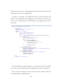
It is important to bear in mind that a constant current produces a
constant torque regardless of speed and given a constant load (constant
torque) the speed of a motor only depends on the voltage applied to it.
The maximum power (product of torque and speed) is produced at the
operating point of half the no-load speed together with half the stall
torque, although due to thermal considerations, a DC motor will not
normally operate at maximum power. When supplying a constant voltage
the speed and torque are inversely related so that the higher the torque
that the motor is forced to develop, the lower the speed will be. Last, for
lower noise generation and better life characteristics the motor should be
chosen with higher voltage ratings than the voltage supply, and when
using with gearing it should be selected for the minimum speed [30].
Types of DC motors
Brushed DC motor
These are a classical example of DC motors. The stator generates a
permanent magnetic field that surrounds the rotor either with permanent
magnets or electromagnetic windings whereas the rotor is made up with
one or more windings. The rotor receives current through a commutator
and carbon brush assembly, hence the term “brushed” (fig. 18).
35
Figure 18: Two-pole brushed DC motor
With brushed DC motors, on one hand it is simple to modify the speed
of the motor by applying different voltages, so in order to make it rotate
faster one only has to increase the voltage. On the other hand, however, if
the user wants to rotate it in both directions it is necessary to build a
controller, an expensive option unless it is possible to build an H-bridge.
It is possible to use pulse width modulation (PWM) to increase/ decrease
the speed without compromising the power, which is a better option than
changing the voltage. A square signal acts, in essence, as a variable
average voltage. These motors are cheap, small and easily controllable but
they produce a relatively low torque [31].
Brushless DC motors
In this type of motor the rotor is a permanent magnet whereas the
stator is an electromagnet. Instead of using brushes, commutation is
achieved electronically so in order to detect changes in orientation
brushless motors generally use Hall-effect sensors to detect the rotor’s
magnetic field. These motors are more expensive than the previous kind
because of their design complexity and they need a controller to control
the speed and rotation.
36
Figure 19: Floppy-Disk brushless DC motors
They are more efficient and have a longer life thus being more capable
for robotic applications providing more torque and speed than brushed
motors. They are usually found in floppy-disks (fig. 19) and other lownoise devices [31].
Stepper motors
Basically a sub-type of brushless motors, stepper motors only have
more magnetic poles on the stator. They convert a pulsed digital input
signal into a discrete mechanical movement and require a special
controller for the current to be applied in the desired sequence. The rotor
is made up of sometimes hundreds of magnetic teeth and it does not
move in a continuous fashion but in discrete steps, thus the name stepper
motor. They are used in many industrial control applications that require
accurate positioning with low-time response [31].
37
Servomotors
These are brushed motors integrated with a control system that enables
precise positioning as they are built coupled with a feedback control
circuitry. The way to control them is by PWM and the typical positional
and speed feedback devices are encoders, resolvers and potentiometers.
They also incorporate a gear system to increase the torque and decrease
the speed [31].
Servomotors, unmodified, do not exhibit continuous rotation and are
used for various purposes from robotics, CNC machinery, automated
manufacturing and RC devices. They are used for higher performance
needs compared to stepper motors.
Their input is a signal that can be either analog or digital and it
represents the position commanded for the output shaft. The difference
between servos and the previous DC motors is that these are closed-loop
mechanisms that incorporate circuitry and gearing.
Figure 20: Industrial servomotor
38
As mentioned before, servomotors are widely used in the industry due
to their high performance in relation to accurate positioning, speed, and
torque. Plus, they usually incorporate error control circuits (figure 20).
For non-industrial inexpensive solutions, there are also massproduced servos suitable for any engineer or electronics amateur available
from $2 to a range of $100-$200, offering a relatively good performance in
most cases. They were commonly used in radio control devices (RC), but
have had a huge increase in the world of small robotics.
These servos have a potentiometer for measuring the position of the
output, and from the comparison between that position and the
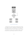
commanded position an error signal is generated to drive the motor. The
servo will stop moving when it reaches the zero-error position (a PWM
commanded position) (fig. 21).
Figure 21: Servo block diagram
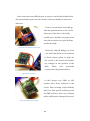
Servo hacking
As for these small versatile servos, it is common practice to use them
for continuous rotation projects such as robot wheels, or robot arms that
need to rotate more than the servo’s limited angle range since most
standard servos allow the shaft to be positioned only between 0 to 180
39
degrees. In order to do this, users have to modify some mechanical and
electrical components of the servo. Each servo has its differences, so the
way to achieve this varies from servo to servo.
First, one should eliminate any mechanical stops that the shaft, gears or
potentiometer may have in order to let the shaft rotate beyond a full
revolution.
Second, it is necessary to cancel the feedback that the circuit sends to
the DC motor through the potentiometer, eliminating the electrical
connection between this and the circuit that controls the DC motor. The
potentiometer, however, should be kept as it normally is part of the shaft
or the shaft itself.
These are the common steps to modifying servos, but the way it is
achieved may vary from model to model. Next, some common parts
found in a servo.
Figure 22: Common servo parts
40
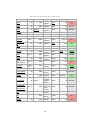
Table 3: Widely used servos and their features [32]
Make Model
Modulati
Weight
on
TowerPr
Analog
o MG995
TowerPr
o SG5010
Align
DS610
Analog
Torque
1.94 oz
4.8V:
(55.0 g)
1.34 oz
(38.0 g)
(10.0 kg-cm)
4.8V:
4.8V:
(8.0 kg-cm)
4.8V:
(9.6 kg-cm)
Digital
4.8V:
6.0V:
Hextroni
Analog
k HXT900
Hitec HSAnalog
645MG
1.95 oz
(55.2 g)
4.8V:
(1.6 kg-cm)
4.8V:
Analog
(3.0 kg-cm)
4.8V:
(2.4 kg-cm)
4.8V:
Analog
$8.90
Coreless
Titaniu
m
$67.99
Coreless
Plastic
$49.99
0.12 sec/60°
Coreless
Plastic
$3.65
0.24 sec/60°
3-pole
Metal
$39.95
3-pole
Plastic
$12.95
3-pole
Plastic
$24.99
Coreless
Titaniu
m
$98.98
3-pole
Plastic
$24.99
0.20 sec/60°
0.19 sec/60°
0.15 sec/60°
0.28 sec/60°
0.22 sec/60°
4.8V:
(18.0 kg-cm)
0.19 sec/60°
6.0V:
(24.0 kg-cm)
Futaba
S3010
Plastic
0.07 sec/60°
6.0V:
6.0V:
1.45 oz
(41.0 g)
3-pole
4.8V:
(3.0 kg-cm)
Hitec HSDigital
5955TG
0.09 sec/60°
6.0V:
6.0V:
2.17 oz
(61.5 g)
$11.95
4.8V:
(3.5 kg-cm)
Futaba
S3001
Metal
0.08 sec/60°
6.0V:
6.0V:
1.59 oz
(45.0 g)
Coreless
4.8V:
(7.7 kg-cm)
(9.6 kg-cm)
Hitec HSAnalog
311
Price
4.8V:
6.0V:
1.52 oz
(43.0 g)
0.10 sec/60°
6.0V:
(2.5 kg-cm)
4.8V:
Mater
ial
4.8V:
(1.9 kg-cm)
0.32 oz
(9.1 g)
Type
0.14 sec/60°
6.0V:
(12.0 kg-cm)
Align
DS520
Street
4.8V:
6.0V:
0.91 oz
(25.9 g)
0.17 sec/60°
6.0V:
(11.0 kg-cm)
Digital
0.20 sec/60°
Gear
4.8V:
6.0V:
1.85 oz
(52.5 g)
Speed
Motor
4.8V:
0.15 sec/60°
4.8V:
(5.2 kg-cm)
6.0V:
0.20 sec/60°
6.0V:
(6.5 kg-cm)
0.16 sec/60°
Recently, it is also possible to purchase continuous rotation servos so
that we can avoid tampering with them, but these are more expensive and
not as common as the limited range servos.
41
Locomotion issues
When designing a robot, we should first consider the way we want it to
move through its environment and how it should accomplish it,
depending on what advantages and disadvantages each locomotion type
has and how they suit our robot’s requirements. [33]
Legged locomotion. Often inspired by biological systems, these kinds
of mechanisms are very successful in moving through a wide area of harsh
environments but often have problems with stability, complexity and
power consumption. A legged robot is well suited for rough terrain, since
it is able to cross gaps, climb steps and cross obstacles so it usually is the
right choice when there are ground irregularities.
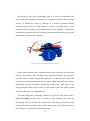
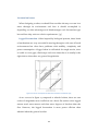
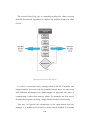
Figure 23: Power consumption of different locomotion mechanisms [33]
As we can see in figure 23 compared to wheeled robots, these are two
orders of magnitude more inefficient on a hard, flat surface since legged
motors need more motors and thus more degrees of freedom than the
first. However, the legged locomotion is more power efficient than
wheeled when the ground is softer.
42
Stability is also an important issue. From 1 leg to n legs, including 2, 4
and 6 (normally based on animal or insect movements) static and
dynamic stability is a complex engineering challenge, certainly more
difficult than the wheeled robots case.
Wheeled locomotion. This is the most popular method for providing
robot mobility. It is normally more power efficient, and requires a simpler
mechanical approach, less motors and it is stable most of the time. There
are robots with two wheels, with a third stable point, but it is more
common to find 4-wheeled robots for better traction (sometimes more 6
or more wheels). Stability here is not a major problem, but there are other
issues worth mentioning. The focus on research in wheeled robotics is on
traction, stability on rough terrain, maneuverability and control.

Stability: It is only necessary that the center of gravity is on the
stability polygon.

Maneuverability. If the movement is differential, (turning is
achieved by powering the wheels at different speeds) the robot will
be omnidirectional. If the robot has an Ackermann steering
configuration, used by cars, the vehicle will have a turning radius
larger than itself, which results in less maneuverability.

Controllability. The disadvantage of the differential configuration
is that controlling the robot becomes harder than with the
Ackermann configuration. For example, it is difficult to keep the
robot in a straight line compared to standard vehicles since these
use the same power for both wheels.
43
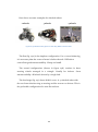
Here there are some examples for wheeled robots:
2 wheels
3 wheels
4 wheels
Figure 24: (a) Wheeled robot; (b) Kovan robot & (c) NASA’s wheeled robot.
The first (fig. 24a) is the simplest configuration. For a correct balancing,
it is necessary that the center of mass is below the axle. Difficult to
control but good maneuverability. Cheap and small.
The second configuration (shown in figure 24b) consists in three
steering wheels arranged in a triangle. Usually for indoors. Great
maneuverability. All wheels driven by a single belt.
The last Image (fig 24c) shows NASA’s rover. A 4-wheeled robot with
the two front wheels acting as steering and the rear two as drivers. This is
the preferable configuration for non-flat surfaces.
44
2.4.
Smartphone Applications
Over the past few years, the market of touchscreen mobile devices has
experienced an enormous growth to the extent that, according to the last
surveys [34], around half of the US mobile consumers own smartphones.
The European mobile market as measured by active subscribers of the
top 50 networks is 860 million and the rate of smartphone adoption is
accelerating, and is soon expected to reach a third of the sales [35].
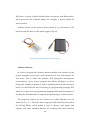
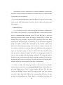
A smartphone is a mobile phone built
on an operating system, with more
advanced computing capability than a
feature phone (media players, camera,
GPS, internet browsing, etc.).
Although the term was coined years before, the real push that opened
this market was the original iPhone by Apple Inc. in 2007, one of the first
mobile phones to use a multi-touch interface. After, in July 2008, Apple
announced its second generation phone with 3G support. By then, the
App Store reached over 1000 million downloads in the first year having
started with only 500. Two more versions of the iPhone have been
released so far, being Apple the leading company in all aspects from
design to functionality [36].
Following the success of the Apple’s App Store other smartphone
manufacturers soon launched their own software application stores, such
as Google’s Android Market or Blackberry’s App World between others.
45
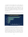
The Applications market is highly attractive for small companies and
third-parties. In 2012, the Apple’s Store recorded $5782 million of
revenues, relatively high compared to other competitor’s stores. This
could be attributed to having the largest number of applications or apps
available as well as the highest download volume in 2010. Also, only 28%
of the apps in the Apple Store were free compared to the 57% in the
Android Market [37].
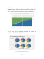
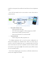
In the next image we can see how deep the smartphone share is in each
market:
Figure 25: Smartphone share per region
As we can see, the leading market for smartphone sales is the Japanese
market, followed by the American market. The special case of Japan can
be explained by their early and massive use of mobile devices, with more
rotation than in other markets and always 3 or 4 years ahead. In Japan,
almost all technological advances are in more widespread than in other
countries and the smartphone market has never been an exception for
46
this. Forecasts are optimistic about a complete penetration of
smartphones for all mobile device users as we can see next (by the end of
2014 an 80% of population is supposed to be carrying a smartphone):
Figure 26: US smartphone penetration
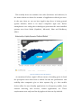
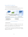
In the rising years of smartphone technology the software and
hardware market had the next distribution:
Figure 27: Software and hardware platform pie
47
We can see that both in software and hardware markets, Apple has
experienced a notable growth while Nokia has decreased its share
accordingly. It is important to remember that before the smartphone era,
Nokia was the undisputable leader and Apple was not even a player in
this market.
Nowadays, however, Apple’s iOS and Google’s Android are the two
biggest competitors in both number of applications and market share,
which translates into smartphone sales as users perceive the availability
and utility of the applications software as a key factor for a mobile device
election. Also, in the last 2 years tablets have joined this hardware market
competing in the same application stores. Tablets are intended for
different reasons (with less portability, bigger screens, less connectivity)
but share almost all apps with smartphones.
The next chart shows the number of applications in each store for every
of the last years.
Figure 28: Apps available per platform
48
This actually does not translate into sales (hardware and software) in
the same relation as shown for number of applications offered per store.
In the next chart we can see how Apple’s App Store is losing ground
against Android, which is its major competitor right now. Before
smartphones were ruling the technological panorama the most installed
systems were from Nokia (Symbian), Microsoft, Palm and Blackberry
(Rim).
Figure 29: Platform market development
As mentioned before, Apple’s iPhone meant a breaking point in both
the perception users have from a mobile OS and the performance and
usability that companies give to their systems (fig 31.). New mobile
devices allow for user-friendly applications in all aspects possible, from
internet browsing, web services, camera applications, etc. These
requirements were only met first by Apple and also now by Android.
49
In conclusion, with this information we can foresee an attractive
future for investors and developers in the applications software
environment.
Smartphones
are
becoming
more
than
just
a
communicating tool to become all-in-one devices with which we can
control and monitor any other electronic devices subject to wireless
communications.
At this point, when developing applications most companies choose
building multi-platform applications for both Android and iPhone. Both
operating systems are widely used and cannot be set aside. However there
are big differences in both worlds while developing and programming
that should be noticed.
On one hand, Android is completely open source, has a large
community of developers and is a light-weight operating system. It is
completely free to start developing for it, and has a vast database of
resources available on the internet, but applications should be runnable
by many different devices, with different hardware configurations and
computing power.
On the other hand, the iOS for iPhone is only intended to work in
iPhones thus making it easier for developers to develop focusing less on
hardware requirements and more on code. It is a proprietary system
available only for Apple’s devices and it costs $99 to become an iOS
developer and purchase the complete developing toolset (version for
developers outside Apple).
50
Chapter 3
Design and manufacture
Although one of the main concerns of
this project is providing robots with the
capability of teleoperation, there has been
no better way of carrying this out than
building the robot itself, allowing for
great versatility and full understanding
between both the commanding part and
the robot. This is also a substantial and
important part, since we determine how the robot is going to physically
behave according to how we implement the control and programming.
By being able to design the robot from scratch we try to simplify its
mechanic behavior allowing for a m0re robust prototype in the sense that
we can focus on the main issues rather than having to deal with
unwanted working areas, such as behavior against obstacles, energy
efficiency, high torques or accelerations, degrees of freedom or even less
the appearance of the machine. Nevertheless, by designing the robot with
the simplest way of movement, which is two wheels, we do not lose the
flexibility that a more complex topology might provide. Instead, it can
51
change speed and direction almost instantly when commanded and at the
same time assuring reliability.
3.1.
3D modeling and design
For the purpose of designing and modeling the structure of the
different parts of the robot there are different tools available, each having
their advantages and disadvantages, as mentioned in the background
chapter.
For this project it has been decided that OpenSCAD is the best choice
since it focuses on the computer aided design aspects instead of the
artistic aspects. This software is entirely open source, and a very powerful
parametrical tool that works by rendering scripts (fig 32). This way,
programmers build their models with parametrical code and the software
compiles the scripts and renders the object. The great advantage of this
program is that by being parametrical users can modify their objects’
attributes by changing certain values of their code. However, this is also a
disadvantage since it makes it more complicated to create objects
compared to other alternatives.
Figure 30: A look into the OpenSCAD software [8]
52
As we can see, on the left side we type the code of the piece, while in
the right side, we can see the rendered result. The objects are created
using mathematical basic functions, from which, we can achieve more
complex shapes.
Among the locomotion systems previously discussed, for this project,
the 2-wheeled option has been selected in order to focus on other aspects
of the robot, such as communications and interfaces, so that we can have
the smallest robot to test (approximately 5 cm long) as well as the
cheapest configuration.
There are 7 pieces modeled for this project’s design. Some are created
as new structure pieces and others are only 3D models of real objects like
servos or the electronic board. Next, we describe each in detail.
Real objects 3D models:
-
LiPo battery. Model of a lithium polymer battery for placing it
under the robot. This will be discussed in a later section.
Figure 31: View of the LiPo battery
-
Servos. After measuring all the distances of the servos, we build a
3D object that represents them accurately, in order to serve as a
guide to design and develop the structure objects of the robot.
53
Figure 32: 3D representation of a TowerPro sg90
-
Electronic Board. There is also an accurate 3D representation of
the board also needed for the construction of the structure pieces.
Figure 33: 3D view of the Arduino Fio board with the RN-XV on it
Structure objects:
As the servos are built opposite to one another, with nothing between
them, they will constitute the main core of the structure so that the
pieces that are going to be designed should basically hold the servos
together firmly. The designed structural pieces should also be able to hold
the electronic board, the Wi-Fi board and the battery always minimizing
the complexity and number of pieces involved.
54
-
Front part. This is a simple piece and it is destined to hold the
front ends of the servos together by having two holes prepared for
ISO metric M2 screws. There is no need for threads because the
screw fits firmly in the holes.
Figure 34: View of the front part
-
Rear part plug. In the back of the robot we have two complex
pieces. The rear part plug serves as a grip for the back part of the
servos, with holes for M2 screws, and at the same time it works as
a plug for the electronic board which fits tightly into the piece.
This is actually the only way of assembling the electronic board
since it does not come prepared for bolts or any other way of
fastening.
Figure 35: 3D model of the rear part plug
-
Rear part support. This part is destined to serve as a third support
for the rear weight of the robot, aside from the wheels. It also fits
within the rear part plug using the same screws.
55
Figure 36: Rear part support
There is a modification of this part which has a marble destined
to roll in any direction the wheels go. However, a more simple
way is preferred, in which this rear support simply slides. The
force of friction is insignificant since the robot weighs very little.
-
The wheels. The wheels are designed so that the servos’ plugs fit
into the wheels very tightly, having for this purpose a hole similar
to the plugs. These wheels also have a decrease in the radius of
their center so that we can place a rubber O-ring to enhance the
grip.
Figure 37: Top view of a wheel
56
In this design it has always been a priority to give the robot an easy
maintenance and functionality so that it is not necessary to
disassemble it for operations like changing or charging the battery,
reprogramming the board, attaching or detaching the wheels and making
any cable connection. All of these procedures can be done keeping the
robot assembled and intact.
In the next picture we have an unassembled view of the robot, in which
there is a better understanding of each piece separately.
Figure 38: Unassembled complete robot
It is also worth saying that some pieces have been redesigned several
times until they have met the requisites of the 3D printer. Not all shapes
57
and angles can be printed because of the working process of the 3D
printer which is adding layers from bottom to top in order to create the
object.
Finally, no matter how precisely we design the pieces to fit together we
will always need some retouching in the sense that sometimes the
precision of the printer is lower than the precision needed for all pieces to
fit. Therefore, some smoothing is needed on some pieces’ edges and
holes.
3.2.
Additive manufacturing or 3D
printing
Once the pieces are designed, the next step is manufacturing the
designed pieces. This is accomplished by a machine called a 3D printer.
The STL files are then opened by a program called ReplicatorG [38] (fig.
42) which serves as the main interface for operating the 3D printer. With
this software we place the object in the adequate “printable” way (always
with the largest part at the bottom) and then translate the STL code into
GCode [39] which is the machines operative code. This code carries the
information of how the printer will move and the order of the steps. [40]
See figure 41.
After the GCode is generated we have to indicate some of the printer’s
options. Although it allows us to choose among many variables the two
most important of them are the platform’s temperature and the extruder
temperature.
58
Figure 39: OpenSCAD to STL format and STL to G-Code [40]
The platform is the base on which the object will be laying and should
be about 120 ºC. The extruder melts the plastic at 220 ºC and makes the
plastic go through it as a fine strip.
Figure 40: A view of the software Replicator G [40]
59
After setting up the printing parameters with this program we
command the printer to start working. Each piece takes, on average,
about 20 to 30 minutes to be printed, which makes, for the entire robot, 1
hour and 40 minutes.
The material from which they are made in this case is called ABS
(acrylonitrile butadiene styrene) and comes in a coil prepared to feed the
printer. It is an inexpensive material, if we consider the €/g, compared to
other manufacturing materials.
In the next picture we can take a look at the printer while building one
of the wheels. As we can see, it works by adding layers from bottom to top
using the extruder as starting point of the melted polymer.
Figure 41: 3D printer building a wheel. [40]
60
3.3.
Assembly
The next and last step of the manufacturing process is the assembly of
the pieces once they all have been printed. However, first and as
mentioned before, some pieces need their surfaces and edges to be
smoothed in order to fit with the others.
When they are ready, we put together the two servos with their ends in
opposite sides and attach to them the front and rear pieces using two
screws for each one of them. After this we can plug the electronic board
into the rear piece.
For the battery we use a sheet of Velcro placed under the servos. This
way we can attach and detach the battery easily and as many times
needed. In the next picture we can see the results so far:
Figure 42: Preassembled robot
Prior to assembling the electronic board we have to solder the male
headers in order to start working with the pins. Next, we assemble the
rear part support, the wheels, and the Wi-Fi board.
61
The complete model
After all the pieces are assembled together, we can take a look at the
final layout of the robot’s design, a 3D model of the complete robot in
which one of the wheels has been removed for a better view.
Figure 43: Assembled complete robot
Figure 44: Top view of the assembled robot
62
Chapter 4
Servomotors and servo hacking
For the robot’s wheels, we have to
choose a pair of servos that suit our
needs. They should be small enough,
so that the we have the lowest power
consumption and make the smallest
robot possible with the tools at hand.
All of this in line with the previously
designed small parts of the robot.
Apart from the obvious specifications that we must seek in any servo
such as torque, speed, voltage, ect. Another element to bear in mind
while choosing a servo is budget. There is actually a huge variety of
different servos offering similar features, and almost all of them could suit
our robot’s demands, so these are not really important at the time of
choosing one servo or another. However, depending on the fiability that
they provide, prices vary within a considerable range.
As mentioned in the first parragraph, the most important feature that
we look for in a servo is size. The world of electronics is constantly
developing devices with enhanced features but smaller sizes and the new
63
generation of servos is not an exception. Although with less fiability, users
can find in the market much smaller servos than before and even build
their own controlling circuits for small DC motors using cheap affordable
components.
Apart from the hardware (servos and electronics), it
is important to remember that a limiting factor for
reducing the robot’s size is the accuracy with which
the printer builds each piece. If we try to build pieces
that are two small, the printer will not build them with
the right accuracy.
As this project focuses on communications and building the controlling
interface, we could allow ourselves to choose a small cheap servo, only
with the necessary features to move the robot. This is the TowerPro’s
SG90, a lightweight servo, which for the price, is very high-quality and
fast.
It comes with accessories for attaching, and has two holes for screws. In
the picture below, we can se these holes on the sides of the servo. It is to
these fins that we attach the front and rear parts of the robot, using
screws to hold them together.
This ~$5 servo, which we can see in the introductory picture has one
big disadvantage, shared with other similar medium-quality servos, which
is that it requires time, effort and skills to modify it in order to make it
rotate 360º. It is possible that upgrading to more expensive but
continuous rotation servos is more worthwhile, in order to avoid all the
trouble related to modifying the structure of these servos. However, it
serves as a learning tool both in mechanics and analog electronics.
64
4.1.
Continuous rotation modification
First, we have to get the four bottom screws out which will let us
disassemble the top and bottom plastic parts:
Figures 45, 46 [41], 47, 48 & 49: Unscrewed and modified servo
After this we have to remove three
mechanical stops. First, two metal fingers in
the potentiometer must be cut using a small
screwdriver to lift the metal plate and then cut
its ends with a diagonal cutter.
Figure 47: Mechanical Stops [41]
Next we remove the other mechanical stop
which is a small nub on the bottom of the
output gear, using a cutter this time but being
careful not to break it. This way, the gear will
be able to rotate freely.
Figure 58: Output gear [41]
After removing the mechanical stops
we have to reassemble the potentiometer
and every gear in the right order engaging
the motor’s gear.
Figure 5: Gear train [41]
65
Now comes the most difficult part. In order to cancel the feedback that
the potentiometer puts into the circuit we have to modify its electronic
behavior:
First we cut the three wires that go
from the potentiometer to the circuit
(red arrow). We have to be really
careful not to desolder any other wires
since the tin unions are quite delicate
and break easily.
Figure 50: Potentiometer's wires [42]
Below the chip (H-bridge) we leave
3 tin ends that must be reconnected
to fixed resistor values in order for
the circuit to be closed and dismiss
any changes in the position of the
shaft.
These
were
previously
connected to the potentiometer.
Figure 51: Tin ends [42]
In this picture two SMD 2.2 KΩ
resistors have been soldered to the
circuit. This is actually a quite difficult
task if we lack specific soldering tools
for SMD resistors, since any common
solder will break or damage the board.
Figure 52: Soldered resistors [42]
66
To solve this problem two common 1/4 W resistors have been used
being really careful not to damage any part while soldering the resistors
legs. However, this method has one big disadvantage; the new circuit with
these resistors will not fit into the servo’s box so the only way possible is
to make a hole in the box and let the resistors out through it.
In conclusion, it is possible that this part of the project could be
reconsidered because of its complexity and difficulty, in the sense that we
could avoid the technical trouble involved in this in favor for a better
performance servo. The only disadvantage would be an over cost for each
servo.
67
68
Chapter 5
Electronic hardware and
programming
In this part, we will cover everything
related to the election and use of all
electronic devices involved in the
robot. In order to make the robot
work
and
move
we
need
a
microcontroller destined to serve as
the main “intelligence”; it deals with
the possible inputs or outputs that the robot may implement, for
example, activities such as running the servos, communicating with other
devices or algorithm execution.
For this specific project, we also need a communicating module that
will deal with the data transfer between the microcontroller board and
the controlling device. This module might or might not come
incorporated to the main board, meaning that we have the possibility of
either an integrated solution or two separate but compatible devices for
the microcontroller and communicating module.
69
The first choice must be the microcontroller. As mentioned in the
background part, the best choice for a low-budget starting project with no
professional requirements would be a microcontroller from the Arduino
family.
5.1.
Microcontroller
Now, depending on our project we should choose the adequate model
that fit exactly with the robot’s power, size and I/O requirements.
First we should know the minimum amount of I/O pins that the robot
needs, so that there are enough digital and analog outputs for the servos
and other controlled devices. In order to provide connectivity, the board
should also allow for an external Wi-Fi, Bluetooth or RF module and they
should be compatible.
Another factor to consider is the necessary computing power needed
for receiving instructions, computing the algorithm and commanding the
servos at the same time with the minimum lag. Any 32-bit microprocessor
should be enough for this task.
For now, we still have several boards that suit our needs, most of them
being more than enough for our needs, but if we want the microcontroller
to be as small as possible our choices narrow a lot.
For these reasons the FIO [43] model has been chosen, which is an
Arduino board intended for wireless applications (fig. 55).
70
Figure 53: Arduino FIO
In the previous picture we can see a top view of the board, with the
microprocessor in the middle and the I/O pins on the sides.
The Arduino Fio is a microcontroller based on the ATmega328P
running at 8 MHz and at 3.3V (fig. 56). It has 14 Digital inputs and
outputs and 8 analog inputs, an on-board resonator, a reset button and a
socket for XBee modules. XBee is a standard pin-arrangement from DIGI
for its RF and Bluetooth modules but it has been adopted by other
companies so that we can find other maker’s modules with different
features all having the same pin arrangement.
Figure 54: ATmega328P [16]
71
It has connections and a USB internal charging circuit for a lithium
polymer battery.
Summary
Table 4: Arduino FIO features
Microcontroller
ATmega328P
Operating Voltage
3.3V
Input Voltage
3.35 -12 V
Input Voltage for Charge 3.7 - 7 V
Digital I/O Pins
14 (of which 6 provide PWM output)
Analog Input Pins
8
DC Current per I/O Pin
40 mA
Flash Memory
32 KB (2 KB used by bootloader)
SRAM
2 KB
EEPROM
1 KB
Clock Speed
8 MHz
Memory
This microprocessor has 32 KB of flash memory for storing code (of
which 2 KB are for the bootloader. It has 2 KB of SRAM and 1 KB of
EEPROM.
Input and output
All 14 pins can act as digital output or inputs with an internal pull-up
resistor of 20-30 k (disconnected by default). They operate at 3.3V and
provide or receive a maximum of 40 mA. Some pins have the next special
functions:
72
-
Serial: RXI (D0) and TXO (D1). Used to receive (RX) and
transmit (TX) TTL serial data.
-
PWM: 3, 5, 6, 9, 10, and 11. Provide 8-bit PWM output with
the analogWrite() function.
-
SPI: 10 (SS), 11 (MOSI), 12 (MISO), 13 (SCK). These pins support
SPI communication.
-
LED: 13. There is a built-in LED connected to digital pin 13.
-
8 analog inputs with 10 bits of resolution.
Communications
The ATmega328P provides UART TTL serial communication, available
on pins 0 (RX) and 1 (TX). This serial connection can be monitored by the
Arduino software through the serial monitor in which we can see the
serial data sent to the Arduino from the computer and vice-versa. This
should be done with a 3.3V FTDI cable. The mini-USB that comes with
the board is only for charging the battery and not for uploading
programs. For further use of the Serial communications interface we can
use the SoftwareSerial library.
The ATmega328P also supports I2C and SPI communication. For I2C
we should include the Wire library in the Arduino software. For the SPI
communication we need to check the datasheet.
The board was designed by Shigeru Kobayashi and manufactured by
SparkFun Electronics.
73
5.2.
Microcontroller programming
In order to start using the board we must solder either the male or
female headers on the board. In this case we soldered a row of male
headers per row of I/O pins.
When it comes to programming the board we have two options: With
an FTDI cable or wirelessly which only works with a pair of DIGI’s RF
modules. As this project uses another board it is a must to program it
with the cable.
After this, we start developing the sketch or Arduino program. As
mentioned before, there are two functions that we must implement in
any program. However, before the first function we include the necessary
libraries for our program, and then we write the setup() and loop()
functions. First, in the setup() function we will initialize the variables,
attach one digital output for each servo, and configure the software serial
connection for carrying out the serial monitoring. (This will be explained
along with the softwareSerial library).
In the setup() function we also set the data rate for serial data
transmission with serial.begin(9600). A working value for the Arduino
FIO is 9600 bps (bits per second).
In the loop() section we will write the main algorithm in charge of
receiving the instructions from the smartphone and commanding the
servos. We read char values from the corresponding Arduino FIO buffer,
which come from the default serial connection with the Wi-Fi module.
As the values received from the Wi-Fi module and sent to the Arduino
are treated as characters, we need to implement a char to int
transformation prior to executing any code that uses the received data.
74
The values sent from the Wi-Fi module to the Arduino are numbers
from 0 to 180 coming from the commanding device (In this case an
Android phone) that represent the desired servo speed. The algorithm
then, groups any incoming char data in separate strings (to differentiate
separate values) and converts the strings into integer values with the
atoi() function.
Only after we have the data converted to an integer we can start
developing the main algorithm which is in fact very simple, excluding a
few issues. As we will receive information to move two separate servos,
but there is only one data channel (Wi-Fi board) and only one buffer for
the serial connection, we have to transform the data so that the Arduino
program knows which servo it is intended to. To achieve this, we send
values from different ranges being each range associated to one servo.
From the smartphone’s application software values are sent from two
different special sliding buttons, one for each servo. Both values travel
through different listeners but are already sent with different ranges as
there is only one channel.
The next image shows the flow chart of the steps explained above. It is
a simplified flow of events that sum up the algorithm behind the robot.
75
Figure 55: Main Arduino block diagram
Inside the “receive string and convert to integer” box there is also a subroutine in charge of doing that task. The next image shows the flow chart
for this task.
76
Figure 56: Block diagram for storing string and converting to integer
When sent to the Arduino from the Wi-Fi module, a number can have
from 1 to 3 digits. Each digit is sent separately and treated as a character.
As the Arduino buffer allows for only one variable to be stored in it, we
have to build a loop that first reads that incoming value, and then stores
77
it in the first position of an array. If there is more incoming data, that is to
say, another number’s digit, we place it in the next position of the array.
As we do not know how many digits the number will have we still have
an array with a variable number of elements which are undetermined,
with no assigned value. In order to use the function atoi() which only
works with a NULL ended string, we have to fill the remaining positions
with NULL values or “\0”. We then convert the string to an integer and it
is ready to be read as a valid number for a servo.
After the data is written to the servo we clean the buffer for the next
loop with serial.flush(). It is important that we add a delay of 10 ms
between the data is being written in the serial buffer and when reading
the data. This way we allow the buffer to have completed before we read
any values.
Regarding the servos, from two of the digital pins capable of providing
PWM signals we connect each servo’s control wire whereas the other two
go to the power supply, in this case, the battery. Servos have 3 wires:
GND, VCC and signal (PWM control). Next we discuss more in deep how
to write values to the servos in the loop() function.
In order for our program to deal with servos, we have two options: We
could either write PWM signals by software as explained in the servo
controlling section of the background chapter or use an available
standard servo library (Servo.h). To simplify the program, in this project,
the library option has been chosen. This library allows for attaching or
detaching a servo to and from any digital pin, as well as writing a value to
the servo controlling the shaft accordingly. For this we could either use
the function write() or writeMicroseconds(), being the latter more
precise.
78
On standard servos a value from 0 to 180 will command a position for
the shaft, and on continuous rotation servos this will set up a speed, being
90 the value of no movement.
It is worth mentioning that near-end values (o to 20 and 160 to 180)
could not be well differentiated as many servos achieve full speed with
lower values.
Technical issues
It is necessary to notice that this specific hardware configuration
(FIO + RN-171 Wi-Fi module) is especially difficult to work with since they
use for communicating the same serial (TX and RX) pins as used for
uploading sketches. Here comes the biggest disadvantage of these two
modules when used together. Despite all the advantages that come when
choosing the FIO board (size, connectivity, ect.) it has been thought for
being used with a DIGI’s XBee Bluetooth or RF module, which even
allowed for wireless programming, so if we want to connect it to the WiFi module we will have to put up with some difficulties when making it
work. As mentioned early, we have to detach the Wi-Fi module every
time we want to upload a sketch, but this is not the biggest trouble. In
order to start working with the module and check for incoming data we
should use the serial monitor that comes with the Arduino IDE. However,
the default serial pins are being used for data transfer to/ from the Wi-Fi
module so that we cannot monitor this flow of information.
In order to solve this issue and achieve data transfer and proper
monitoring we should use the softwareSerial.h library which allows for
any other digital pin to serve as serial transfer (RX and TX). We then
connect the RX and TX from the FTDI cable to these new pins and the
rest (VCC, GND, ARef and DTR) to the corresponding FIO pins. For this
we have to disassemble the FTDI cable. In conclusion, we have two
79
running serial communications at the same time, one for monitoring the
buffered read values, and other for communicating with the Wi-Fi
module.
Layout
The next picture shows the electronic configuration of the robot. It is
quite simple, only taking care in powering the servos with the battery and
not with the Arduino, which can only supply 40 mA.
Figure 57: Robot, servos and battery layout
80
5.3.
Wi-Fi module
After considering the pros and cons of the two main options for
providing connectivity (Bluetooth or Wi-Fi), it has been decided that the
best choice would be the Wi-Fi module. The advantages are data with
ultra-low cost transport, the biggest connectivity range (if using local area
networks with access point we can connect to everywhere in the world),
and a greater versatility providing many different configurations. This
way we have the possibility to interact with any device that is connected
somehow to the network. A significant factor is that between 2009 and
2010 there was a 158% growth in Wi-Fi enabled consumer electronics and
it was present in 90% cell phones [44].
The best choice is the Roving-Networks RN171XV (fig. 60), which is a
standalone, complete TCP/ IP wireless networking module. Due to its
small size and low power consumption it is perfect for mobile wireless
applications such as sensing and portable devices. It is the best option for
projects migrating from existing 802.15.4 architecture to a standard 802.11
TCP/ IP based platform without any changes in their existing hardware.
Figure 58: Roving-Networks RN-XV 171 Wi-Fi module [29]
81
The module incorporates a 32-bit processor, TCP/ IP stack, real-time
clock, crypto accelerator a power management unit and analog sensor
interface.
It
also
offers
additional
functionality
through
its
8
programmable GPIOs (general purpose input/ output) and 3 ADCs. The
ADCs provide 14-bit resolution while the GPIOs can be configured to
allow standard functionality or status signaling to a host microcontroller
minimizing the need for serial polling between the module and the
microcontroller.
Among all the features (See manual, or main web site), we can outline
some important ones:
-
Based common 802.15.4 footprint.
-
Access to every node. Ad-hoc and AP configurations.
-
Low power
-
3.3V supply
-
Secure Wi-Fi authentication
-
Configuration over UART or wireless interface (telnet) using ASCII
codes.
For this project the module has been connected to the Arduino
hardware with the simplest configuration, only using PWR, TX, RX and
GND for communicating with the microcontroller: A common serial
communication. This is showed in the circuit layout in the 3.2 section.
The module has an endless set of applications and lets the user set
multiple configurations according to their needs. To begin with there we
will offer a general overview of the configuring commands, default
features and working modes. Later we will see some typical applications
82
in which to incorporate the module and some hints on how to implement
them.
First of all, the module can be in two modes or states: Data mode or
command mode:
Figure 59: Wi-Fi module operating modes [44]


Data mode (default state).
-
WiFly module like data pipe.
-
TCP/ UDP header stripped or added, transparent to UART.
-
Data written to UART is sent out to Wi-Fi.
-
Data received from Wi-Fi is read from UART.
Command mode.
-
Used to assign data, SSID, pass phrase, etc.
To configure parameters and/ or view the current configuration, we
must put the module into command mode. There are various ways to
connect to the Wi-Fi module and enter in command mode for the first
time. In all of them, the user has to establish connection with the module
and send the escape sequence $$$. If the module answers CMD it means
we are in command mode.
Note: In the configuring part, next section, we will take a look at how to
connect and configure the module.
83
Upon entering the command mode, the module can accept five types of
commands:
-
Set commands: These take effect immediately and are stored in
memory. They include the categories shown in table 5.
Table 5: Set commands parameters
-
Get
commands:
These
commands
retrieve
the
stored
configuration and display it. They are basically the same
commands as the “set commands” but take no parameters.
Instead, they show the current configuration.
-
Status commands: These commands display the interface
status, the IP status, etc.
-
Action commands: for scanning, connecting, disconnecting,
etc.
-
File I/O commands: to upgrade, load and save configuration,
delete files, etc.
84
Some possible Wi-Fi applications
TCP connections and embedded applications
We can connect from/to module to/from host using TCP. In the next
image we can see the typical applications for this module (fig. 62).
Figure 60: Typical TCP applications [44]
Roaming and FTP
Used for asset tracking, fleet management and remote sensor
applications. The configuration is more complicated than the previous
one and combines broadcast UDP, wake timers and auto join.
The module can act as an FTP client streaming files to/from FTP server
(useful in data logger applications), and as an FTP server accepting
multiple clients concurrently.
85
The next image shows this configuration:
Figure 61: FTP client/ server configuration [44]
HTML client and sensors
In the next image we can see the architecture for this application:
Figure 62: HTML client configuration [44]
86
With this configuration we can post data to a web server associating the
module to an access point. (The image shows RN-370 modules but this
also works with the 170 series). In HTTP client mode the module sends
the next request message, including comm remote string and sensor
readings:
GET /server.php?value=0F3000001111222233334444555566667777\n\n
When serial UART data arrives the module auto-connects to web server
and sends.
Access point mode (AP mode)
In addition to infrastructure and Ad-hoc mode, the module can act as
an access point, providing several advantages over Ad-hoc mode:
-
The module creates an AP network to which Android devices can
join.
-
The module runs a DHCP server and issues IP addresses to seven
clients, which is much faster than automatic IP and Ad-hoc mode.
-
The module supports routing between clients.
There are two methods for enabling AP mode, hardware and software.
To enable it in hardware, we must hold the GPIO9 to 3,3V and then reset
the module. It starts with the next default AP mode settings:
Table 6: Default access point mode settings
87
To enable it via software we use the next commands. After the first we
do not need to enter them in the same order.
set wlan join 7
// Enable AP mode
set wlan channel <value>
// Specify the channel
set wlan ssid <string>
// Set up network broadcast SSID
set ip dhcp 4
// Enable DHCP server
set ip address <address>
// Specify the IP address
set ip net <address>
// Specify the subnet mask
set ip gateway <address>
// Specify the gateway
save
// Store settings
reboot
// Reboot the module in AP mode
Once the module boots up in AP mode, any client device can associate
with the network the module is broadcasting. Once associated, the
module DHCP server assigns an IP address to the client device.
Ad-hoc mode
An Ad-hoc network is a point-to-point network in that each Wi-Fi
device is linked directly to all other devices on that network with no
access point. All devices participate in keeping the network alive and each
keeps track of the other active devices on the network by sending and
receiving beacon and probe packets. In most cases, IP addresses are
assigned through automatic IP, although one of the Wi-Fi devices can be
configured as a DHCP server. There are also two ways to enable Ad-hoc
mode.
88
The first, via hardware, we set GPIO9 high at power up. Upon
powering up with that pin high, the module creates an Ad-hoc network
with the next settings:
SSID
WiFly-GSX-XX, (XX is Mac address)
Channel
1
DHCP
OFF
IP address
169.254.1.1
Netmask
255.255.0.0
Via software, we introduce the next commands:
set wlan join 4
set wlan ssid “name”
set wlan chan 1
set ip address 169.254.1.1
set ip netmask 255.255.0.0
set ip dhcp 0
save & reboot
Once a computer is associated with the Ad-hoc network, we can use
the module’s IP address to open a connection or connect using telnet.
89
5.4.
Wi-Fi module programming
The following part of the document explains how to configure and
program the WiFly module (RN-171) to connect it to a WLAN and act as a
server for any Android device to talk to it via TCP.
This chapter is a summary of an extended tutorial by
the same author of this document on how to use and
configure the module with Arduino. It can be found at
http://asrob.uc3m.es/index.php/Tutorial_Wifly,
a
Spanish step-by-step tutorial for programming the
module for the first time.
Among the many ways possible for the module to work (acting as
access point, Ad-hoc or infrastructure) it has been decided that it would
be appropriate to configure it to connect to a local network providing it
with a static IP so that it would be reachable at all times and would have a
wide coverage in a certain spot. Besides this is a much simpler
configuration than making it broadcast its own wireless network.
However, this last option (acting as an access point) would mean that we
could use the robot in any place without the need for an external wireless
network. The disadvantage of configuring it as an AP is a lower coverage
area (less than 10 m).
The module will be configured so that it rapidly connects to a router at
power up. Apart from the Wi-Fi module, we will use the next tools:

Ubuntu

Arduino FIO

WiFly Manual and datasheet

FTDI 3,3V cable and a small thin wire.
90
We will show three different ways to configure and achieve the same
results. The first will be via hardware (and then telnet) and the last two,
software. Configuration parameters will be stored in the module’s
memory so that every time it reboots it can auto-connect to the router.
Hardware and telnet
First of all, we enable the WiFly’s Ad-hoc mode by connecting GPIO_9
(8th pin of the XBEE’s pinout to VCC (3,3v, 1st pin). See images below:
Figure 63: GPIO_9 to VCC & Figure 64: Module powered by FIO
Figure 65: Wire for short-circuiting GPIO_9 to VCCC.
91
By forcing it enter in Ad-hoc mode we can connect to it via telnet for
the first time and then configure it. There is also a software way to
configure it in Ad-hoc but we must first establish contact with it by
forcing a hardware Ad-hoc.
When powered up with the FTDI cable from a computer through the
Arduino FIO (it could be from the battery) we should see the three LEDs
on (amber, red and green). This means the connections are correct.
Second of all, we should try to reach its network. According to the
manufacturer, the default values are:

IP: 169.254.1.1

Netmask: 255.255.0.0
This Netmask means that if we want to reach its net we should have a
169.254.XXX.XXX type of IP, being XXX any number from 0 to 254 (except
for 1.1 which is the address of the module itself).
Once powered up we should wait (perhaps some minutes) until we can
see WiFly-GSX-XX on the available wireless networks list on Linux (topright corner, connection configuration). The last two XX are the last two
bytes of the modules MAC address. Once it shows up (Fig. 68) we go to
edit connections and select the WiFly-GSX-XX inside wireless and edit it.
Inside the wireless tab we select Ad-hoc and leave everything else intact.
In the wireless security tab we select none (for simplicity reasons) and in
the IPv4 tab we select manual method and click on add in address.
92
Figure 66: Wireless connection configuration
At this point we have to set an IP for our computer that is inside the
subnet ranged by 255.255.0.0. For example we can set an IP of 169.254.1.1
and a Netmask of 255.255.0.0. We then save the changes and connect to
WiFly-GSX-XX.
Once connected, we open a prompt (Linux terminal) and ping to
169.254.1.1. This way we check if we can send and receive TCP packets to
that address. If everything goes well we should receive data. To exit we
press ctrl + c.
Now it is time to configure the module. From the terminal we type:
telnet 169.254.1.1 2000 which starts a communication with the module
using the telnet protocol. (By default the module listens for telnet
93
connections on port 2000). Once we open the connection the module
answers “HELLO”.
After the connection is opened we type $$$ without carriage return (to
enter in configuration mode) and should receive “CMD”. We are now
ready to configure it by typing the next commands followed by “enter”.
set wlan auth 0
set ip dhcp 0
Open network, no authentication.
DHCP off: It will not ask for an IP or gateway.
set ip adress X.X.X.Y.
We set the WiFly’s IP.
set ip host X.X.X.Z.
The router’s IP. (Same subnet).
set ip netmask 255.255.255.0.
set wlan ssid "name".
set wlan channel 0.
It will look in every channel.
set wlan join 1.
Automatically join the stored ssid.
After this we save and rebot.
save.
reboot.
The next time we power the Arduino with the WiFly module plugged
in, it will reach for the router’s network and connect to it using the
assigned static IP.
Arduino IDE and library
On the internet we can find some libraries (written in C) destined to
work with the WiFly module (WiFlyHQ [45], WiFlySerial [46], WiFly,
etc.) and they all work in a similar way. The most complete and robust is
94
the WiFly-Shield library [47]. To install it we have to download it and
decompress it creating a libraries folder in the sketchbook, inside the
Arduino folder. (“~/sketchbook/libraries/”). This library comes with some
example codes for Arduino (Client, Server, FTP, HTTP, etc.). To use it in a
sketch we have to write #include<WiFly.h>.
In order to start working with it we write the next setup() function:
Within this initialization setup
function,
we
will
use
the
WiFly.begin() function to enter in
command mode and connect to
an external server to get the time
and date. We should comment
this part of the code in the
WiFlyDevice.cpp file.
With the different Serial.begin()
functions we initialize the serial
ports. With the SoftwareSerial.h
library we enable different TX
and RX pins for serial comm. We
also enable the UART to be able
to communicate with the Wi-Fi
module serially.
With the join() function we
establish
communication
with
the ssid and passphrase specified
in the credentials file.
95
In order to make this work we need two FTDI cables. The first powers
the Arduino FIO and loads the program to the board using the standard
TX and RX serial pins, which also communicate with the Wi-Fi module
through Serial.print(). The second cable only needs its yellow and orange
wires to act as software RX and TX and will connect (through another
USB port) to the defined pins by the SoftwareSerial object. See figure 69.
Figure 67: Layout for serial communication
96
Data flowing through this second cable will be showed in the serial
monitor of the Arduino IDE. For this purpose we could have a loop()
function as follows:
With this function, any data
coming
through
the
Wi-Fi
module will be read by the FIO’s
UART and written to the serial
monitor through the second TX
and RX (Software serial pins).
When the setup() sketch is run, the serial monitor shows the module’s
assigned IP with serialTest.println(Wifly.IP()). If we telnet to that IP and
to port 2000 any data written with the line of commands from Linux will
be quickly showed in the serial monitor (fig. 70).
Figure 68: Telnet communication between Laptop and Wi-Fi module
97
This way we have established, through Arduino, a configuration,
connection and data streaming.
Next, the last way to configure the Wi-Fi module.
Directly with Arduino Sketch and IDE
This last method for configuring the module is the simplest in terms of
external help as we do not use libraries or extra material apart from the
Arduino board and the Wi-Fi module. However we are required to dig
into the user’s manual and add a little bit of complexity to our code.
We will write a code in which the serial functions write() and read()
will communicate with the Wi-Fi module using the UART. (Let us recall
that this serial pins are the standard pins for serial communications,
usually used for monitoring data and uploading sketches). This way, we
use the same pins that the Arduino uses for talking to the module for
uploading our program to the Arduino memory.
This program automatically sends to the Wi-Fi’s module a set of
instructions similar to the ones used in the first method. The same
instructions that we use to configure it by telnet can be written to the
UART and then serially read by the WiFly. The only precaution that we
must take is that we should leave a few milliseconds between each
instruction so that it can take effect.
98
Next, goes the check() function, which waits for the module to respond
to each instruction and stores it in an array. Then, it prints this answer to
the serial monitor.
99
As loop() function we can use the same as found in the second method.
Last, it is important to notice that we send the character ‘\r’ as line feed
for the instructions to take effect (unless we send the $$$ command to
start configuring the module, which does not go with \r).
100
Chapter 6
Android application software
This project focuses mainly in building a
software
application
robotic
machine.
for
In
controlling
particular,
a
the
application controls a wheeled robot but it
is possible to generalize the contents and
functionality of this software to extend it to
other types of robotic control (robot arms,
humanoids, industrial machinery, etc.).
It has been developed for Android with the possibility of being run by
smartphones and tablets with wireless internet connections.
Java was the preferred language for this project, although as mentioned
in the background section it is possible to write parts of the code in both
C and C++. The code has been written using Linux (Ubuntu distribution)
and Windows both with Eclipse as IDE (integrated developing
environment). Almost all features of the final application have been
previously tested in an Android virtual device (AVD) where developers
can check the behavior of their applications before installing them in a
real device. There have been parts, however, that could not be run in an
101
AVD such as connectivity with other devices (TCP sockets) and some
multi-thread code.
Before developing for Android directly, it has been the intention of this
project to fully understand the possibilities given by the Java language
when interacting with external electronic devices (Arduino) using
sockets, and at the same time, understand the way data is transferred
through a TCP connection and how it is treated by the Arduino board.
This is covered in the next subsection.
As explained before, all data transferred to the Wi-Fi module, either
using Bluetooth protocols or TCP/IP protocols is treated always as
characters.
For this reason, although we send integers with one or more digits, it is
from the Arduino software side that we must implement a routine, if we
need it, to convert these characters or strings into integers.
102
6.1.
Java GUI
In order to test and demonstrate the communications with the Wi-Fi
module and Arduino, a Java program has been built using simple TCP
connections and a Java graphic user interface to interact with the servos.
The two most important console commands both in Windows and
Linux to work with Java are Javac for compiling .java code and Java for
running the resulting .class compiled file (fig. 71):
Figure 69: Console commands for running Java
Note: it is important that we have previously installed the Java platform
(Java SE), which includes the Java Development Kit (JDK) and the Java
Runtime Environment (JRE) to run applications (More on this in the next
section) [48].
With the first command we compile the code. After compiling, and if
there has been no error, with the second command we launch the
program. In the next image we can see the resulting Java GUI, which is a
103
simple window with two controllers (sliders) that send information to the
Arduino (fig. 72).
Figure 70: Java User interface program for robot control
This Java Application creates a socket and acts as a client in order to
send the data to the Arduino (server, listening for incoming data).
What is a socket? A socket is one endpoint of a twoway communication link between two programs running
on the network. A socket is bound to a port number so
that the TCP layer can identify the application that data
is destined to be sent. An endpoint is a combination of an
IP address and a port number [49].
The Client-side knows the hostname of the machine on which the
server is running and the port number on which the server is listening
(fig. 73).
Figure 71: Client-server connection: client request [49]
104
The server-side: If there is no error in the connection, the server
accepts the connection and gets a new socket bound to the same local
port. It keeps the socket open so that it can continue to listen for client
requests (fig. 74).
Figure 72: Client-server connection: server accepts connection [49]
Next, some captures of the Java code necessary for this application. In
the first capture we create and show the window containing the program.
private static void createAndShowGUI() {
//Create and set up the window.
JFrame frame = new JFrame("sliders");
frame.setDefaultCloseOperation(JFrame.EXIT_ON_CLOSE);
Sliders animator = new Sliders();
//Add content to the window.
frame.add(animator, BorderLayout.CENTER);
//Display the window.
frame.pack();
frame.setVisible(true);
//animator.startAnimation();
}
In the next capture we create and configure the Sliders. The class
constructor of JSlider allows for initial, minimum and maximum values
that will be sent through the socket.
105
//Create the sliders
JSlider rightSlider = new JSlider(JSlider.VERTICAL,
MIN_RIGHT, MAX_RIGHT, INIT_RIGHT);
JSlider leftSlider = new JSlider(JSlider.VERTICAL,
MIN_LEFT, MAX_LEFT, INIT_LEFT);
rightSlider.addChangeListener(this);
leftSlider.addChangeListener(this);
//leftSlider.setMajorTickSpacing(10);
//framesPerSecond.setPaintTicks(true);
6.2.
Android developing platform
In order to start developing for Android it is recommended to
download the ADT Bundle (Android Developer Tools) [50]. It includes
the Android SDK components (Software developing kit, a comprehensive
set of development tools, a debugger, libraries, sample codes, etc.) and a
version of the eclipse IDE with built-in ADT. This project has been
developed completely under Eclipse, since it is the officially supported
IDE. Some parts have been done in Linux and others in Windows.
Under Linux we must follow the next steps to have all packages
configured and ready: After downloading the SDK we untar the .tgz into
an appropriate location which we will refer to later when setting up the
ADT plugin. The next step is downloading the ADT plugin and once
Eclipse starts we must specify the location of our ADT directory. This
plugin extends the capabilities of Eclipse to let us quickly set up Android
projects, build an app UI, debug it and export app packages for
distribution.
Now if we are running a 64-bit system we must install the ia-32 libs
package using apt-get (Ubuntu):
ubuntu : ~$ apt-get install ia32-libs
106
After, we install Java:
ubuntu : ~$ apt-get install oracle-java7-installer
Now, we have to launch the SDK manager and install the last Android
platform and the latest SDK platform-tools. This is because the original
SDK package includes only the SDK tools.
In the next picture we can see the SDK manager, which we can launch
from Linux just by typing sdk in the command line.
Figure 73: Android SDK manager [50]
When the Android tools are updated or a new version is released, we
can use the SDK Manager to quickly download them to our environment.
107
6.3.
Basics of apps development
Once we downloaded and installed the set of tools included in the SDK,
we can access them form the Eclipse IDE. The basic steps for developing
applications are shown in figure 76.
Figure 74: Basic steps for apps development [50]
108
Setup
During this phase we install the development environment (2º part of
this chapter) and create our Android virtual device (AVD)
Development
We develop our source code and include all media files needed for the
application (video, photo, music, etc.).
Debugging and testing
In this phase we build our project into a debuggable .apk that we can
install or run on the emulator. We can also test the application using
various SDK Android testing tools.
Publishing
The last step is building the application for release and distributing it.
In this project we will focus in the first two parts. First, we will see how
to set up an Android virtual device followed by how to install the
application on a real Android hardware, and last, we will cover the
building and running.
Managing virtual devices
First, from Eclipse we launch the AVD manager (fig. 77) which is an
emulator configurator that lets us model an actual device by defining
hardware and software options to be emulated by the Android emulator.
We can select a hardware profile for hardware features, for example, if it
has a camera, a physical QWERTY keyboard, memory options and so on.
109
Figure 75: AVD Manager [50]
Through this window we create and configure as many virtual devices
as we need. It is important that we test our application on different
devices with different screens and features to enhance the application’s
performance.
Using hardware devices
First we have to declare our application as debuggable in our Android
manifest. (This step is automatic with Eclipse). After this, we have to
enable USB debugging under Settings > Applications > Development. Last,
we have to set up our system to detect our device.
Under Ubuntu Linux we have to add a udev-rules file that contains a
USB configuration for each type of device. Each device manufacturer is
identified as a unique vendor ID.

First, we log in as root and create this file:
/etc/udev/rules.d/51-android.rules
We should use the next format to add each vendor to the file:
SUBSYSTEM=="usb", ATTR{idVendor}=="0bb4", MODE="0666", GROUP="plugdev"
110

Then execute:
chmod a+r /etc/udev/rules.d/51-android.rules
Building and running
When building an application Android projects are compiled and
packaged into an .apk file containing the compiled .dex files, a binary
version of the manifest and compiled and uncompiled resources.
The following diagram shows the components involved in building and
running an application:
Figure 76: Project phases [50]
Before we run our project we should be aware of a few important
directories and files in the Android project.
AndroidManifest.xml
This file describes the fundamental characteristics of the app and
defines each of its components. We define how the resources are going to
be displayed and how each feature will behave. Also, we specify the
activities and services that will run in the application and the target
Android version.
111
Src/
This is the directory for our app’s main source files.
Res/
This folder contains several sub-directories for app-resources, for
example:
Drawable/
Directory of the drawable objects (bitmaps) included.
Layout/
Files that define our app’s user interface.
Inside this folder we will put all images (drawable objects, .jpg, .png,
etc.) and the .xml files containing the layout information for each activity.
In Android, every app is built with activities or services. An activity is
an application component that provides a screen with which users can
interact to perform different actions. Every activity is given a window
with a user interface. Every time that we open a new “window” from the
classic computers point of view that window is an activity. When we
transition from one screen to another, with different components and
functions, we change from one activity to another.
Another application component of the same hierarchy is a service. A
service can perform long-running operations in the background (but in
the same thread) but does not provide a user interface.
112
Managing the activity lifecycle
The Android system, unlike other programming paradigms which
implement a main() method, initiates code in an activity instance by
invoking specific methods that correspond to different stages of its
lifecycle. There is a sequence of methods for starting the application and
other sequence to tear it down (fig. 79). This two make a sequence similar
to a step pyramid being the top of the pyramid (resumed) the point at
which the activity is running and the user can interact with it.
Figure 77: Activity lifecycle [50]
Depending on the complexity of our activity we probably do not need
to implement every method of the lifecycle as the system normally
manages them if they are not specifically defined. In the paused state,
the system is partially obscured by other activity and cannot receive any
input or execute any code.
In the stopped state the activity is completely hidden and not visible to
the user (background). The instances and activity information is retained
but cannot execute any code.
113
The created and started states are transient and the system quickly
moves from them to the next state. After the system calls onCreate(), it
quickly calls onStart() followed by onResume().
The onCreate() method is invoked when the user selects the app icon
from the Android system and it is equal to a main method (launcher
method). The onCreate() method should define the user interface as well
as basic application startup logic.
Transitions between the other states are done by invoking the
functions between them (Figure 79) but are normally not specifically
defined as the system does that automatically (for example, if we do not
implement the onDestroy() method, the system will destroy all local class
references from memory when no longer needed).
This project’s main application only defines the onCreate() method for
building the user’s interface, buttons, and other objects. The rest of the
methods are managed by the system while users run the activity.
However, for the second activity (controlling activity), we manually
define the onStart() method for creating a second thread (apart from the
main) in charge of sending cycling chain values for controlling the robot.
In the next section of this chapter we will take a look at the two
activities (Main activity and Control activity) involved in the application,
their function, some significant pieces of their code and the block
diagram for each of them.
114
6.4. Application for robot control
This project’s application consists of two Activities and two different
threads for the second activity.
First, upon launching the application we have an initial screen (for the
first activity) in which we can introduce an IP and port for later
connecting to a robot using that address. If we do not introduce anything,
the application will use default values. This first activity acts as an
introductory screen, and the only thing left to do there is pressing a
button to change to the controlling activity (fig. 80).
Basically, the user decides when to start controlling the robot, so the
connections are not going to begin until the second activity is launched.
It is a “waiting room” for the Android–robot interaction to begin running.
Figure 78: Main activity and Control activity
115
As we can see in the previous image, these two activities form the
Android application.
6.4.1.
Main activity
When launched (fig. 81), the application starts with this activity,
defining so in the Manifest as the main activity (this way Android keeps
record of the activities’ hierarchy in the AndroidManifest.xml). It only
serves as an introductory screen from which users can introduce an IP
and a port, (different from default) that will be transferred to the second
activity for connecting to the robot.
Figure 79: Main activity’s graphical layout
116
The code for this activity is very simple, only having the onCreate()
method and an event object that relates a button to the second activity.
The controlling button (middle of the screen) starts the second activity
and leaves this one behind. Within the onCreate() constructor, we set the
rules for the layout (path to xml file) and the objects to build in the
screen.
Next, the block diagram for this activity:
Figure 80: Block diagram for the Main activity
When the control button is pressed, the control activity is launched. In
the next section we will explore in detail this second activity.
117
6.4.2.
Control activity
In this activity users perform two important actions. First, with the
connect button we can start the communications. The program opens a
socket with either the previously specified address or the default IP and
port. In the middle of the screen there is a text box that serves as a log for
monitoring the sequence of actions that the program runs.
As we can see in Figure 83, the layout for this activity is in landscape
mode by default so that it is easier to control using the thumbs. With the
upper button we connect and with the bottom button we disconnect.
Figure 81: Graphical layout for the Control activity
If connected successfully, a “connection accepted” message will appear
in the log showing the socket’s IP and port. If there is an error, the log will
try to catch the exception produced and will show the corresponding
118
error. We then, can associate the message to a specific cause and try to
solve it. This log text-box is able to auto-scroll when new messages are
written and do not fit anymore. This way there is always room for more
messages and users are able to scroll upwards to read previous messages.
In the next image we can see the code in charge of that function:
There is also a disconnect button to close the socket. This is always
recommended and considered a good practice before closing the
application, so that we do not leave a sleeping process in memory or a
useless open connection.
Next, the code for opening the socket and connecting the seekbars’
values (integers subject to be sent to the Arduino) to the socket’s
associated output object (socket.getOutputStream()). Apart from opening
a TCP channel (as client) with the Arduino (server) we relate the
constantly changing values from the seekbars to the output buffer of the
socket (object that sends information to the server). If we needed to
implement a two-way connection, we would use also an InputStream
object (associated to the socket as well) to receive information from the
server. This would be interesting if, for example, we were required to read
119
field data from sensors or third applications (web services) and use that
incoming data in our main application.
As this is a prototype, we should first focus on the main issues and
build a robust application by debugging errors involved in this process.
Later on, we could expand the functionality of the application as well as
the robot.
public void InicioConexion (View view) {
if (!conectado) {
Log("Intentando iniciar conexión...");
Log("IP: " + IP);
Log("Puerto " + puerto);
try {
socket = new Socket(IP, puerto);
Log("Conectado con Arduino");
try {
salida = new PrintWriter(socket.getOutputStream(), true);
} catch (Exception e) {
// TODO Auto-generated catch block
Log("error print-socket");
try {
Thread.sleep(4000);
} catch (InterruptedException e1) {
// TODO Auto-generated catch block
e1.printStackTrace();
}
e.printStackTrace();
}
conectado = true;
} catch (UnknownHostException fallo) {
Log("No ha sido posible conectar - UnknownHostException");
Log(fallo.getMessage());
conectado = false;
} catch (IOException fallo) {
Log("No ha sido posible conectar - IOException");
Log(fallo.getMessage());
conectado = false;
}
} else {
Log("ya estas conectado");
}
}
The codes showed in this document are a minor part of the complete
code, but are also fundamental for the application and worth analyzing.
Next, the block diagram for this second activity together with the
second thread for communications.
120
Figure 82: Control Activity block diagram
This program runs in the user’s interface main thread and any changes
in the seekbars are written in a variable that is accessible from the second
thread through a pipe that connects both threads. It is not possible for a
second thread to access (read or write) any variable or instance created in
the main thread so a special binding is required between both threads.
121
The second thread (fig. 85) is constantly sending the values received
from the first thread, regardless of whether any seekbar changes its value
or not.
Figure 83: Second thread's block diagram
In order to control the robot, sending values to the Wi-Fi module, this
implementation is not the only one possible. Indeed, there are other ways
with different advantages and disadvantages to approach the issue of
commanding a robot with numeric values. For example, the first way to
develop the program was using a single thread for the second activity.
This way, we opened the connections in the main thread and any
changes in a seekbar were treated as events which resulted in instantly
122
writing the seekbars values in the output buffer, and then being sent to
the robot. This was a simple solution from the Android side but an
ineffective one for the robot since values were sent with no separation
from one another making it incapable of distinguish different numbers.
3 4 36 40
3
Android
43
6
40
Robot
This resulted in an erratic movement.
There was also another problem; we could not solve this from the
Arduino side (robot) making it sample two-cypher numbers because the
range covered numbers from one to three cyphers.
This implementation was the fastest but resulted inefficient. A solution
for this problem came with the second implementation: Instead of
sending a value for every event launched by the seekbars class listeners,
we could only send a value when a seekbar stopped moving, that is, when
users released their thumb from the screen (assuming they use that
finger). This assured that values where sent isolated from one another
making it impossible to create an overlapping in the data transfer.
However, there was a problem with this. Users did not get a fluid
feeling when controlling the robot since they had to release and touch
back again the screen with every change in direction, making it both
rough and uncomfortable.
The third improvement was simple; we could make the change listeners
wait a short delay before sending a value to the output buffer, so that
123
there is no overlapping because the Arduino has time to process a single
value before receiving another. This actually resulted to be really fluid
since users do not perceive this delay (10 ms) which is perfect to create
the right synchronization between both sides of the communication.
The last solution is probably the most professional but also the most
complex of all. As previously mentioned we create a second thread in
charge of a cyclic communication. This way the constantly changing
seekbars and their associated event listeners are isolated from the code in
charge of sending the values through the socket (fig. 86).
50 ms
Figure 84: Multi-threading behavior
The complexity of this last implementation is far greater than the
previous solutions since we are working with multi-threading and its
implications. Although the user does not perceive it, values are actually
sent always every 50 ms, which is a rigid rate, separating the user
commands from the data transfer. This means, we have an indirect
control which could be prejudicial for critical real-time applications.
Actually, this last method has not proved to be 100% solid, since the
application sometimes crashes in some Android devices. This could be,
probably, because of the fact that Android versions behave differently and
treat (or manage) threads and processes differently. Another issue is that
the Android virtual machine does not always behave correctly when
working with multi-threading applications.
124
Chapter 7
Conclusions and future work
Within the boundaries of this project and
regarding its purposes in relation to
manipulating low level wireless electronic
modules as well as open source hardware
and software (both Arduino and Android),
we can assume that many of the initial
goals have been accomplished resulting in
an almost fully printable robot subject to
teleoperation from any place in the world with an accessible Wi-Fi
network. Nevertheless, almost none of the fields developed in this project
can be considered in a dead-end state, as this is only an initial approach
to the yet theoretical system that is currently under construction: Robot
Devastation.
We are now expecting developers (electronics or computers engineers)
to start digging into this project and pick an area that is yet to be built, as
the UC3M robotics society is always available with the support and tools
necessary for it. Although it may seem an arduous work at first, we
encourage them to join this project, as it is worth the effort to work as
125
part of a bigger project to have an understanding of the different areas
and how they connect between them.
Among all that is left to be developed, we can start by mentioning a few
inner projects that are already theoretically pre-defined (each one up to a
certain point).
First, for example, we would need a group of computer engineers to
build the server system: it should be a robust system in charge of
managing all data at all times (24/7) and it should be accurate in terms of
response time. If we consider Robot Devastation as a game, latency times
should always be reduced to a minimum (which is a difficult task). A
typical situation that we could think of would be an encounter between
two robots (active at the same moment). These two start with life points
and have the ability to aim and shoot the opponent decreasing its life
points. All of this information would be managed from a server to which
robots would constantly upgrade with their status. This status at the same
time would be instantly reported to the user/ operator.
Second, from the electronics side, apart from improving the current
robot (all its features are subject to redesigning for future versions),
someone could provide a future version with sensors to achieve field
information transmissions. Each robot would need a sensor to receive the
shots from others and a shooting device as well. Besides, we could
improve its performance by providing it with solar cells up to a point
where the robot would need to recharge much less often.
As a conclusion to this, there will be a lot of work to do for a long time
in all areas which will favor research and experience to those involved.
126
Figure 85: Concept of Robot Devastation by Santiago Morante
In the picture we can see a possible future version of the smartphone
application in which we can actually see the environment at the time of
playing as well as some augmented-reality objects.
127
128
References
[1] J. González Víctores, "ASROB," May 2013. [Online]. Available:
http://asrob.uc3m.es/index.php/INTERFAZ.
[2] 3ds, May 2013. [Online]. Available: http://www.3ds.com/products/catia/.
[3] Autodesk, "AutoCAD," May 2013. [Online]. Available:
http://www.autodesk.com/products/autodesk-autocad/overview.
[4] Invis, May 2013. [Online]. Available: http://www.inivis.com/.
[5] Newtek, Inc., May 2013. [Online]. Available: https://www.lightwave3d.com/.
[6] Blender foundation, May 2013. [Online]. Available: http://www.blender.org/.
[7] ISTI-CNR, May 2013. [Online]. Available: http://meshlab.sourceforge.net/.
[8] C. Wolf and M. Kintel, May 2013. [Online]. Available: www.Openscad.org.
[9] 3D Systems, May 2013. [Online]. Available:
http://www.ennex.com/~fabbers/StL.asp.
[10] 3D systems, May 2013. [Online]. Available: http://printin3d.com/3d-printers.
[11] A. Bowyer, "RepRap," May 2013. [Online]. Available:
http://reprap.org/wiki/Main_Page.
[12] N. Bilton, "Disruptions: 3D printing on the fast track, NYT," May 2013. [Online].
Available: http://bits.blogs.nytimes.com/2013/02/17/disruptions-3-d-printing-ison-the-fast-track/?nl=todaysheadlines&emc=edit_th_20130218.
[13] H. Blair-Smith, "Back to the moon: NASA," May 2013. [Online]. Available:
http://klabs.org/richcontent/verification/80k85_verification/index.htm.
[14] G. E. (. Moore, May 2013. [Online]. Available:
http://download.intel.com/museum/Moores_Law/ArticlesPress_Releases/Gordon_Moore_1965_Article.pdf.
[15] Wikipedia, "Basic information about CPU architecture," May 2013. [Online].
Available: http://en.wikipedia.org/wiki/Comparison_of_CPU_architectures.
129
[16] Atmel, "AVR," May 2013. [Online]. Available: www.atmel.com.
[17] A. Holdings, "ARM," May 2013. [Online]. Available: arm.com.
[18] Motorola, "MC68000," May 2013. [Online]. Available:
http://www.freescale.com/files/archives/doc/ref_manual/M68000PRM.pdf.
[19] "The Most Widely Used Computer on a Chip: The TMS 1000 State of the Art: A
Photographic History of the Integrated Circuit (New Haven and New York:
Ticknor & Fields)," May 2013. [Online]. Available:
http://smithsonianchips.si.edu/augarten/p38.htm.
[20] O. Jostein Svendsli, " Atmel’s Self-Programming Flash Microcontrollers," May
2013. [Online]. Available: http://www.atmel.com/Images/doc2464.pdf.
[21] Microchip, June 2013. [Online]. Available: http://www.microchip.com/.
[22] Infiniteon, "XC800," May 2013. [Online]. Available: http://www.infineon.com/.
[23] Microchip Technology, "PIC," May 2013. [Online]. Available:
http://www.microchip.com/.
[24] Arduino, May 2013. [Online]. Available: http://arduino.cc/.
[25] June 2013. [Online]. Available: https://www.sparkfun.com/products/11460.
[26] June 2013. [Online]. Available: https://www.sparkfun.com/products/341;
http://sra-solder.com/section.php/139/1/arduino_compatible_solar_cells.
[27] MIT media Lab, June 2013. [Online]. Available: http://www.processing.org/.
[28] DIGI, "DIGI's RF modules," May 2013. [Online]. Available:
http://www.digi.com/products/zigbee-rf-modules/.
[29] Roving-Networks, "Roving Networks RN-171XV," May 2013. [Online]. Available:
http://www.rovingnetworks.com/products/RN171XV.
[30] Micromo, "Micromo: "How to choose a DC motor"," May 2013. [Online].
Available: http://www.micromo.com/how-to-select-a-dc-motor.aspx.
[31] Wikipedia, "DC Motors," May 2013. [Online]. Available:
http://en.wikipedia.org/wiki/DC_motor.
[32] Servodatabase.com, "Servo database," May 2013. [Online]. Available:
130
http://www.servodatabase.com/.
[33] S. Bottcher, May 2013. [Online]. Available:
http://www2.cs.siu.edu/~hexmoor/classes/CS404-S09/RobotLocomotion.pdf.
[34] " "The magic moment: Smartphones now half of all U.S. mobiles"
Venturebeat.com," May 2013. [Online]. Available:
http://venturebeat.com/2012/03/29/the-magic-moment-smartphones-nowhalf-of-all-u-s-mobiles/.
[35] telecomsmarketresearch.com, "Europe's mobile operators look to international
opportunities and LTE for future growth," May 2013. [Online]. Available:
http://www.telecomsmarketresearch.com/resources/Mobile_Market_Europe.sh
tml.
[36] A. I. J. 1. 2. Press Release, ""Apple’s App Store Downloads Top 1.5 Billion in First
Year"," May 2013. [Online]. Available:
http://www.apple.com/pr/library/2009/07/14Apples-App-Store-DownloadsTop-1-5-Billion-in-First-Year.html.
[37] Appleinsider.com, ""Apple's rivals battle for iOS scraps as app market sales grow
to $2.2 billion"," May 2013. [Online]. Available:
http://appleinsider.com/articles/11/02/18/rim_nokia_and_googles_android_bat
tle_for_apples_ios_scraps_as_app_market_sales_grow_to_2_2_billion.html.
[38] "ReplicarotG," May 2013. [Online]. Available: http://replicat.org/.
[39] MIT, "Gcode," May 2013. [Online]. Available: http://carlsonmfg.com/cnc-g-codem-code-programming.html.
[40] ASROB, June 2013. [Online]. Available:
http://asrob.uc3m.es/index.php/Instrucciones_de_impresion_R26.
[41] "SG90 Continuous rotation tutorial," May 2013. [Online]. Available:
http://www.fetchmodus.org/projects/servo/.
[42] "SG90 Electrical modification," May 2013. [Online]. Available: http://www.driguana.com/prj_TPro_SG90/index.html.
[43] S. Kobayashi, "Arduino FIO," May 2013. [Online]. Available:
http://arduino.cc/es/Main/ArduinoBoardFio.
[44] Roving-Networks, "RN171 presentation," May 2013. [Online]. Available:
http://www.rovingnetworks.com/resources/download/150/Wifly_Training_Pres
131
entation.
[45] "GitHub," May 2013. [Online]. Available: https://github.com/harlequintech/WiFlyHQ.
[46] T. Waldock, "GitHub," May 2013. [Online]. Available:
https://github.com/perezd/arduino-wifly-serial.
[47] C. Taylor, P. J. Lindsay, J. Crouchley, B. Breznak and jmr13031, "GitHub," May
2013. [Online]. Available: https://github.com/sparkfun/WiFly-Shield.
[48] "Java Download," May 2013. [Online]. Available:
http://java.com/en/download/index.jsp.
[49] "Java tutorials," May 2013. [Online]. Available:
http://docs.oracle.com/javase/tutorial/networking/sockets/definition.html.
[50] Google, "Android developer tools," May 2013. [Online]. Available:
http://developer.android.com/sdk/index.html.
[51] R. Wilson, ""The Great Debate: SOC vs. SIP". EE Times," May 2013. [Online].
Available: http://www.eetimes.com/electronics-news/4052047/The-GreatDebate-SOC-vs-SIP.
132
Appendices
PROJECT BUDGET
UNIVERSIDAD CARLOS III DE MADRID
Escuela Politécnica Superior
1. Author: Jorge Kazacos Winter
2. Department: Electronic Systems and Automation
3. Project Description: Android Controlled Mobile robot
Duration: 10 months
Indirect costs rate: 20%
4. Budget breakdown
LABOUR COST
Name
Category
Dedicated
time (hours)
Cost per
Hour (€)
Cost
(€)
Jorge Kazacos Winter
Engineer
110
50
5500
Juan González
Víctores
Senior
Engineer
40
100
4000
Alberto Jardón Huete
Senior
Engineer
4
100
400
Total
€9900
133
EQUIPMENT COST
Description
Cost (€)
% of
use
Duration
(months)
Depreciation
period (months)
Attributable
cost (€)
3D printer
600
10
2
60
2
Arduino FIO
20
100
10
60
3.3
RNXV-171
35
100
10
60
5.83
LiPo battery
8.9
100
10
60
1.48
2 SG servos
3.5
100
10
60
0.58
Set of tools
20
100
10
60
0.33
Laptop
800
100
10
60
133.33
Android tablet
300
100
10
60
50
Total
Amortization formula:
Where
(for final cost).
A = Number of months of use of the equipment.
B = Depreciation period
C = Cost of the equipment
D = Percentage of use of the equipment.
And
Indirect cost = 0.2 x (Labour + Amortization)
134
€199.90
COST SUMMARY
Description of total cost
Total cost (€)
Labour cost
9900
Amortization cost
199.90
Indirect cost
2019.98
Grand total
12119.88
135