Download the Software User`s Manual

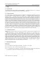
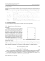
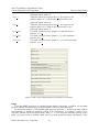
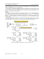
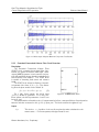
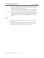
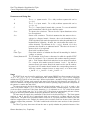
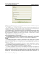
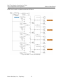
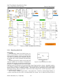
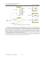
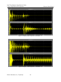
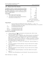
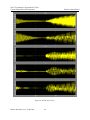
REAL-TIME ADAPTIVE ALGORITHMS FOR FLIGHT
CONTROL DIAGNOSTICS AND PROGNOSTICS
Software Users Manual (SUM)
November 29, 2009
CONTRACT # NNL08AA06C
Jason O. Burkholder
BARRON ASSOCIATES, INC.
1410 Sachem Place
Suite 202
Charlottesville, VA 22901
434-973-1215, Ext. 121
[email protected]
Distribution:
Kenneth W. Eure, Ph.D.
Mail Stop 130
NASA Langley Research Center
Hampton, VA 23681
Gang Tao, Ph.D.
UNIVERSITY OF VIRGINIA
Elec. & Computer Engineering
351 McCormick Road
Charlottesville, VA 22904
434-924-4586
[email protected]
SBIR/STTR Administration Office
Mail Stop 126
NASA Langley Research Center
Hampton, VA 23681
NASA Center for Aerospace Information
Attn: Acquisitions Collections Development Specialist
7115 Standard Drive
Hanover, MD 21076
DISTRIBUTION STATEMENT B - Distribution authorized to U.S. Government Agencies and their contractors. Other
requests for this document shall be referred to NASA Langley.
DISTRIBUTION STATEMENT X - Distribution authorized to U.S. Government Agencies and private individuals or
enterprises eligible to obtain export-controlled technical data in accordance with NFS 1852.225-70.
SBIR Rights: Contract No. NNL08AA06C. Barron Associates, Inc., 1410 Sachem Place, Charlottesville, VA 22901-2496.
In accordance with DFARS 252.227-7018, expiration of SBIR Data Rights is five years after completion of the project,
including any follow-on phases. The Governments rights to use, modify, reproduce, release, perform, display, or disclose
technical data or computer software marked with this legend are restricted during the period shown as provided in paragraph
(b)(4) of the Rights in Noncommercial Technical Data and Computer Software-Small Business Innovation Research (SBIR)
Program clause contained in the above-identified contract. No restrictions apply after the expiration date shown above.
Any reproduction of technical data, computer software, or portions thereof marked with this legend must also reproduce
the markings.
CONTENTS
CONTENTS
Contents
1 Scope
1.1 Identification . . . . . . . . . . . . . . . . . . . . . . . . . . . . . . . . . . . . . . . . .
1.2 System Overview . . . . . . . . . . . . . . . . . . . . . . . . . . . . . . . . . . . . . .
1.3 Document Overview . . . . . . . . . . . . . . . . . . . . . . . . . . . . . . . . . . . . .
1
1
1
1
2 Referenced Documents
1
3 Software Summary
3.1 Software Application . . . . . . . . . . . . . . . . . . . .
3.2 Software Inventory . . . . . . . . . . . . . . . . . . . . .
3.3 Software Environment . . . . . . . . . . . . . . . . . . .
3.4 Software Organization and Overview of Operation . . . .
3.5 Contingencies, Alternate States and Modes of Operation
3.6 Security and Privacy . . . . . . . . . . . . . . . . . . . .
3.7 Assistance and Problem Reporting . . . . . . . . . . . .
4 Access To The Software
4.1 First-Time User of the Software . .
4.1.1 Equipment Familiarization
4.1.2 Access Control . . . . . . .
4.1.3 Installation and Setup . . .
4.1.4 Removal . . . . . . . . . .
4.2 Initiating a Session . . . . . . . .
4.2.1 Toolbox Examples . . . . .
4.3 Stopping and Suspending Work . .
.
.
.
.
.
.
.
.
.
.
.
.
.
.
.
.
.
.
.
.
.
.
.
.
.
.
.
.
.
.
.
.
.
.
.
.
.
.
.
.
.
.
.
.
.
.
.
.
.
.
.
.
.
.
.
.
.
.
.
.
.
.
.
.
.
.
.
.
.
.
.
.
.
.
.
.
.
.
.
.
.
.
.
.
.
.
.
.
.
.
.
.
.
.
.
.
.
.
.
.
.
.
.
.
.
.
.
.
.
.
.
.
.
.
.
.
.
.
.
2
2
2
4
4
4
4
4
.
.
.
.
.
.
.
.
.
.
.
.
.
.
.
.
.
.
.
.
.
.
.
.
.
.
.
.
.
.
.
.
.
.
.
.
.
.
.
.
.
.
.
.
.
.
.
.
.
.
.
.
.
.
.
.
.
.
.
.
.
.
.
.
.
.
.
.
.
.
.
.
.
.
.
.
.
.
.
.
.
.
.
.
.
.
.
.
.
.
.
.
.
.
.
.
.
.
.
.
.
.
.
.
.
.
.
.
.
.
.
.
.
.
.
.
.
.
.
.
.
.
.
.
.
.
.
.
4
4
4
4
5
5
6
6
6
5 Processing Reference Guide
5.1 Capabilities . . . . . . . . . . . . . . . . . . . . . . . . . .
5.2 Conventions . . . . . . . . . . . . . . . . . . . . . . . . . .
5.3 Processing Procedures . . . . . . . . . . . . . . . . . . . . .
5.3.1 Adaptive Actuator Failure Detector . . . . . . . . . .
5.3.2 Multi-Output Adaptive Observer Fault Detection . .
5.3.3 Extended Constrained Kalman Filter Fault Detection
5.3.4 Remaining Useful Life . . . . . . . . . . . . . . . . .
5.3.5 Adaptive Plant . . . . . . . . . . . . . . . . . . . .
5.3.6 Adaptive Sensor Failure Detection . . . . . . . . . .
5.3.7 Stuck Signals . . . . . . . . . . . . . . . . . . . . .
5.3.8 Nonparametric Cumulative Sum . . . . . . . . . . .
5.3.9 Geometric Moving Average . . . . . . . . . . . . . .
5.3.10 Girshick-Rubin-Shiryaev SCD . . . . . . . . . . . . .
5.3.11 Filtered Sliding Window . . . . . . . . . . . . . . . .
5.3.12 Brodsky-Darkhovsky SCD . . . . . . . . . . . . . . .
5.3.13 Generalized Likelihood Ratio . . . . . . . . . . . . .
5.4 Related Processing . . . . . . . . . . . . . . . . . . . . . .
.
.
.
.
.
.
.
.
.
.
.
.
.
.
.
.
.
.
.
.
.
.
.
.
.
.
.
.
.
.
.
.
.
.
.
.
.
.
.
.
.
.
.
.
.
.
.
.
.
.
.
.
.
.
.
.
.
.
.
.
.
.
.
.
.
.
.
.
.
.
.
.
.
.
.
.
.
.
.
.
.
.
.
.
.
.
.
.
.
.
.
.
.
.
.
.
.
.
.
.
.
.
.
.
.
.
.
.
.
.
.
.
.
.
.
.
.
.
.
.
.
.
.
.
.
.
.
.
.
.
.
.
.
.
.
.
.
.
.
.
.
.
.
.
.
.
.
.
.
.
.
.
.
.
.
.
.
.
.
.
.
.
.
.
.
.
.
.
.
.
.
.
.
.
.
.
.
.
.
.
.
.
.
.
.
.
.
.
.
.
.
.
.
.
.
.
.
.
.
.
.
.
.
.
.
.
.
.
.
.
.
.
.
.
.
.
.
.
.
.
.
.
.
.
.
.
.
.
.
.
.
.
.
.
.
.
.
.
.
.
.
.
.
.
.
.
.
.
.
.
.
.
.
.
.
6
6
7
7
7
13
17
22
26
31
35
35
36
38
39
40
41
42
.
.
.
.
.
.
.
.
.
.
.
.
.
.
.
.
.
.
.
.
.
.
.
.
.
.
.
.
.
.
.
.
i
.
.
.
.
.
.
.
.
.
.
.
.
.
.
.
.
.
.
.
.
.
.
.
.
.
.
.
.
.
.
.
.
.
.
.
.
.
.
.
.
.
.
.
.
.
.
.
.
.
.
.
.
.
.
.
.
.
.
.
.
.
.
.
.
.
.
.
.
.
.
.
.
CONTENTS
5.5
5.6
5.7
5.8
Data Backup . . . . . . . . . . . . . . .
Recovery from Errors, Malfunctions, and
Messages . . . . . . . . . . . . . . . . .
Quick-Reference Guide . . . . . . . . .
CONTENTS
. . . . . . .
Emergencies
. . . . . . .
. . . . . . .
.
.
.
.
.
.
.
.
.
.
.
.
.
.
.
.
.
.
.
.
.
.
.
.
.
.
.
.
.
.
.
.
.
.
.
.
.
.
.
.
.
.
.
.
.
.
.
.
.
.
.
.
.
.
.
.
.
.
.
.
.
.
.
.
.
.
.
.
.
.
.
.
.
.
.
.
42
42
42
42
6 Notes
42
6.1 Abbreviations and Acronyms . . . . . . . . . . . . . . . . . . . . . . . . . . . . . . . . 42
ii
LIST OF FIGURES
LIST OF FIGURES
List of Figures
1
2
3
4
5
6
7
8
9
10
11
12
13
14
15
16
17
18
19
20
21
22
23
24
25
26
27
28
29
30
31
32
33
34
35
36
37
ADAPT in Simulink Library Browser . . . . . . . . . . . . . .
Adaptive Actuator Failure Detector Simulink Block . . . . . .
Adaptive Actuator Failure Detector Simulink Block Parameters
State errors: unfaulted case. . . . . . . . . . . . . . . . . . .
State errors: fault in actuator u1 . . . . . . . . . . . . . . . . .
State errors: fault in actuator u2 . . . . . . . . . . . . . . . . .
State errors: fault in actuator u3 . . . . . . . . . . . . . . . . .
Multi-output Adaptive Observer Simulink Block . . . . . . .
Multi-output Adaptive Observer Simulink Block Parameters .
Multi-output Adaptive Observer Component Test Harness . .
Multi-output Adaptive Observer Component Test Results . .
ECKF Simulink Block . . . . . . . . . . . . . . . . . . . . .
ECKF Simulink Block Parameters . . . . . . . . . . . . . . .
ECKF - Linear System Example . . . . . . . . . . . . . . . .
ECKF - Non-linear System Example . . . . . . . . . . . . . .
Remaining Useful Life Block . . . . . . . . . . . . . . . . . .
RUL Block Parameters . . . . . . . . . . . . . . . . . . . . .
RUL Component Test Harness . . . . . . . . . . . . . . . . .
RUL Component Test Results . . . . . . . . . . . . . . . . .
Adaptive Plant Simulink Block . . . . . . . . . . . . . . . . .
Adaptive Plant Block Parameters . . . . . . . . . . . . . . .
Adaptive Plant Component Test Harness . . . . . . . . . . .
Adaptive Plant Component Test Results - x4 . . . . . . . . .
Adaptive Plant Component Test Results - x9 . . . . . . . . .
Adaptive Sensor Failure Detection Simulink Block . . . . . .
Adaptive Sensor Failure Detection Simulink Block Parameters
ADSUF Model . . . . . . . . . . . . . . . . . . . . . . . . .
ADSUF State Errors . . . . . . . . . . . . . . . . . . . . . .
Stuck Signals Simulink Blocks . . . . . . . . . . . . . . . . .
Nonparametric Cumulative Sum Simulink Block . . . . . . .
Geometric Moving Average Simulink Block . . . . . . . . . .
Geometric Moving Average Example . . . . . . . . . . . . . .
Geometric Moving Average Example Results . . . . . . . . .
Girshick-Rubin-Shiryaev SCD Simulink Block . . . . . . . . .
Filtered Sliding Window SCD Simulink Block . . . . . . . . .
Brodsky-Darkhovsky SCD Simulink Block . . . . . . . . . . .
Generalized Likelihood Ratio SCD Simulink Block . . . . . .
iii
. . .
. . .
. .
. . .
. . .
. . .
. . .
. . .
. . .
. . .
. . .
. . .
. . .
. . .
. . .
. . .
. . .
. . .
. . .
. . .
. . .
. . .
. . .
. . .
. . .
. . .
. . .
. . .
. . .
. . .
. . .
. . .
. . .
. . .
. . .
. . .
. . .
.
.
.
.
.
.
.
.
.
.
.
.
.
.
.
.
.
.
.
.
.
.
.
.
.
.
.
.
.
.
.
.
.
.
.
.
.
.
.
.
.
.
.
.
.
.
.
.
.
.
.
.
.
.
.
.
.
.
.
.
.
.
.
.
.
.
.
.
.
.
.
.
.
.
.
.
.
.
.
.
.
.
.
.
.
.
.
.
.
.
.
.
.
.
.
.
.
.
.
.
.
.
.
.
.
.
.
.
.
.
.
.
.
.
.
.
.
.
.
.
.
.
.
.
.
.
.
.
.
.
.
.
.
.
.
.
.
.
.
.
.
.
.
.
.
.
.
.
.
.
.
.
.
.
.
.
.
.
.
.
.
.
.
.
.
.
.
.
.
.
.
.
.
.
.
.
.
.
.
.
.
.
.
.
.
.
.
.
.
.
.
.
.
.
.
.
.
.
.
.
.
.
.
.
.
.
.
.
.
.
.
.
.
.
.
.
.
.
.
.
.
.
.
.
.
.
.
.
.
.
.
.
.
.
.
.
.
.
.
.
.
.
.
.
.
.
.
.
.
.
.
.
.
.
.
.
.
.
.
.
.
.
.
.
.
.
.
.
.
.
.
.
.
.
.
.
.
.
.
.
.
.
.
.
.
.
.
.
.
.
.
.
.
.
.
.
.
.
.
.
.
.
.
.
.
.
.
.
.
.
.
.
.
.
.
.
.
.
.
.
.
.
.
.
.
.
.
.
.
.
.
.
.
.
.
.
.
.
.
.
.
.
.
.
.
.
.
.
.
.
.
.
.
.
.
.
.
.
.
.
.
.
.
.
.
.
.
.
.
.
.
.
.
.
.
.
.
.
.
.
.
.
.
.
.
.
.
.
.
.
.
.
.
.
.
.
.
.
.
.
.
.
.
.
.
.
.
6
7
9
11
12
12
13
13
15
16
17
17
20
21
22
22
24
25
25
26
28
29
30
30
31
32
33
34
35
35
36
37
38
38
39
40
41
Real-Time Adaptive Algorithms for Flight
Control Diagnostics and Prognostics
1
1.1
Software Users Manual
Scope
Identification
This Software Users Manual (SUM) documents ADAPT — the Barron Associates, Inc. integrated
adaptive diagnostic and prognostic toolbox for MATLABR , Version 1.0.
1.2
System Overview
The overall objective of this research program is to improve the affordability, survivability, and service
life of next generation aircraft through the use of ADAPT — an integrated adaptive diagnostic and
prognostic toolbox. The specific focus of the research effort is adaptive diagnostic and prognostic
algorithms for systems with slowly-varying dynamics. Model-based machinery diagnostic and prognostic
techniques depend upon high-quality mathematical models of the plant. Modeling uncertainties and
errors decrease system sensitivity to faults and decrease the accuracy of failure prognoses. However, the
behavior of many physical systems changes slowly over time as the system ages. These changes may be
perfectly normal and not indicative of impending failures; however, if a static model is used, modeling
errors may increase over time, which can adversely affect health monitoring system performance. Clearly,
one method to address this problem is to employ a model that adapts to system changes over time.
The risk in using data-driven models that learn online to support model-based diagnostics is that the
models may “adapt” to a system failure, thus rendering it undetectable by the diagnostic algorithms.
An inherent trade-off exists between accurately tracking normal variations in system dynamics and
potentially obscuring slow-onset failures by adapting to failure precursors that would be evident using
static models. The ADAPT toolbox features an innovative new parameter estimation algorithms and
new adaptive observer / Kalman filter techniques designed specifically for health monitoring.
1.3
Document Overview
This SUM shall document installation and usage of the ADAPT computer software configuration item
(CSCI).
SBIR DATA RIGHTS: Contract No. NNL08AA06C. Barron Associates, Inc., 1410 Sachem Place,
Charlottesville, VA 22901-2496. In accordance with DFARS 252.227-7018, expiration of SBIR Data
Rights is five years after completion of the project, including any follow-on phases. The Governments
rights to use, modify, reproduce, release, perform, display, or disclose technical data or computer software
marked with this legend are restricted during the period shown as provided in paragraph (b)(4) of the
Rights in Noncommercial Technical Data and Computer Software-Small Business Innovation Research
(SBIR) Program clause contained in the above-identified contract. No restrictions apply after the
expiration date shown above. Any reproduction of technical data, computer software, or portions
thereof marked with this legend must also reproduce the markings.
2
Referenced Documents
References
[1] G. Tao, Adaptive Control Design and Analysis.
John Wiley & Sons, 2003.
[2] B. Stevens and F. Lewis, Aircraft Control and Simulation.
[3] G. T. Stephen Mack and J. Burkholder, “Real-time adaptive algorithms for flight control diagnostics
and prognostics,” NASA Final Technical Report, pp. 103–113, November 2009.
Barron Associates, Inc., Proprietary
1
Real-Time Adaptive Algorithms for Flight
Control Diagnostics and Prognostics
3
3.1
Software Users Manual
Software Summary
Software Application
The ADAPT toolbox provides advanced system health monitoring algorithms in the form of Simulink
block components. These components may be used to develop health monitoring applications with the
Simulink modeling tool. The applications can be tested and refined within the high-fidelity Simulink
modeling environment. After verification, the Real-Time Workshop code generation tool may be used
to generate deployable C language code for integration in online real-time health monitoring systems.
The ADAPT algorithms provide out-of-the-box diagnostic capabilities that are applicable to a wide
range of health monitoring problems.
3.2
Software Inventory
The ADAPT software is distributed in either hard or soft format. The hard format distribution is a single
CD with the ADAPT toolbox in the root directory. The soft format distribution is a single compressed
archive with the ADAPT toolbox in the root directory.
The root directory of the distribution contains this user’s manual, the installation script and toolbox implementation. Subdirectories contain the support files, including documentation, examples and
Windows runtime.
Barron Associates, Inc., Proprietary
2
Real-Time Adaptive Algorithms for Flight
Control Diagnostics and Prognostics
Software Users Manual
The root directory contains the following installation files:
AdaptSoftwareUsersManual.pdf
htmlHelpHelper.m
installAdaptToolbox.m
libAdapt.mdl
slblocks.m
This user’s guide.
Integrated HTML help script.
The toolbox installation script.
The ADAPT library.
Simulink library toolbox integration script.
The root directory contains the following implementation files:
aafd callback.m
adaptiveplant callback.m
asfd callback.m
brodsky darkhovsky sfunction.c
brodsky darkhovsky sfunction.mexw32
glr sfunction.c
glr sfunction.mexw32
moao callback.m
rulsfunc.cpp
rulsfunc.mexw32
sliding window filter sfunction.c
sliding window filter sfunction.mexw32
The “Doc” subdirectory contains the integrated help files:
acc09b.pdf
acc10mack.pdf
adaptiveActuatorFailureDetectorHelp.html
adaptivePlantHelp.html
adaptiveSensorFdHelp.html
aiaa08b.pdf
aiaa09b.pdf
BarronLogo.png
contrivedRulTest.png
contrivedRulTestResult.png
demoAafd.png
demoAafdResults.png
demoAdaptivePlant.png
demoAdaptivePlantResults-x4.png
demoAdaptivePlantResults-x9.png
demoAdaptiveSensorFd.PNG
demoAdaptiveSensorFd e.PNG
demoAdaptiveSensorFd faultGen.PNG
demoEnabledStuckSignals.PNG
demoEnabledStuckSignals out.PNG
demoMoao.png
demoStuckSignals.PNG
demoStuckSignals out.PNG
moaoHelp.html
qualifier v4.pdf
rulHelp.html
scdHelp.html
stuckSignalsHelp.html
ADAPT is distributed with a set of simple examples that demonstrate their performance and usage. These examples are designed for a Windows simulation environment, and are not meant as code
generation targets. The “ToolboxExamples” subdirectory contains the toolbox usage examples:
AdaptiveActuatorFailureDetectorExample.mdl
AdaptiveActuatorFailureDetectorExample Initialize.m
AdaptivePlantExample.mdl
AdaptivePlantExample Intitialize.m
AdaptiveSensorExample.mdl
AdaptiveSensorExample Initialize.m
MultiOutputAdaptiveObserverExample.mdl
MultiOutputAdaptiveObserverExample Initialize.m
RulExample.mdl
The “Microsoft.VC80.CRT” subdirectory contains Microsoft C/C++ runtime files with which the
toolbox was built. These files are required to run the s-functions:
Microsoft.VC80.CRT.manifest
msvcm80.dll
Barron Associates, Inc., Proprietary
msvcp80.dll
msvcr80.dll
3
Real-Time Adaptive Algorithms for Flight
Control Diagnostics and Prognostics
3.3
Software Users Manual
Software Environment
ADAPT is designed for the R2007b release of The MathWorksTM products:
Product
MATLABR
SimulinkR
Real-Time WorkshopR
xPC TargetTM
Version
7.5
7.0
7.0
3.3
ADAPT is integrated with Simulink so that it is available in the Library Browser tool.
3.4
Software Organization and Overview of Operation
The ADAPT toolbox is a collection of reusable Simlink blocks in Simulink library form. After installation,
ADAPT appears as a folder within the Simulink library browser. The blocks may be used like any other
Simulink component. Each block has an integrated help page.
3.5
Contingencies, Alternate States and Modes of Operation
Each ADAPT block is designed to be simulated under the Simulink system, as well as allowing code
generation for deployment in real-time applications.
3.6
Security and Privacy
The ADAPT toolbox has no security or privacy issues.
3.7
Assistance and Problem Reporting
Direct all problems and inquiries to the report preparer:
Barron Associates, Inc
1410 Sachem Place, Suite 202
Charlottesville, VA 22901
(P) 434.973.1215
4
Access To The Software
4.1
4.1.1
First-Time User of the Software
Equipment Familiarization
ADAPT is targeted for a standard Windows XP computer.
4.1.2
Access Control
ADAPT has no access control features beyond the operating system login.
Barron Associates, Inc., Proprietary
4
Real-Time Adaptive Algorithms for Flight
Control Diagnostics and Prognostics
4.1.3
Software Users Manual
Installation and Setup
The ADAPT toolbox is distributed as a simple compressed (e.g. zip) file that contains all required
resources. The distribution contains a MATLAB script that installs and cleanly uninstalls the software.
This script executes within the MATLAB environment.
The ADAPT distribution includes the script file “installAdaptToolbox.m”. This script installs and
uninstalls the toolbox. The base installation directory is the Windows “program files” path, which is
defined by the environment variable “ProgramFiles”. This path is the default installation location for
all programs, including MATLAB itself. The script will install the toolbox under the folder “BarronAssociates”, in the subfolder ”ADAPT”. The ADAPT folder will be added to the end of the MATLAB
path, so that the toolbox is accessible by MATLAB and Simulink.
To install the ADAPT toolbox:
1. Extract the toolbox distribution’s compressed contents.
2. Start MATLAB R2007b.
3. Navigate to the directory containing the distribution’s uncompressed contents.
4. At the MATLAB command line, execute the command: installAdaptToolbox
The install script will respond with the following status messages:
>> installAdaptToolbox
Installing ADAPT Toolbox
...creating directory C:\Program Files\BarronAssociates
...creating directory C:\Program Files\BarronAssociates\ADAPT
...creating directory C:\Program Files\BarronAssociates\ADAPT\Doc
...creating directory C:\Program Files\BarronAssociates\ADAPT\ToolboxExamples
...creating directory C:\Program Files\BarronAssociates\ADAPT\Microsoft.VC80.CRT
...copying files to C:\Program Files\BarronAssociates\ADAPT
...copying files to C:\Program Files\BarronAssociates\ADAPT\Doc
...copying files to C:\Program Files\BarronAssociates\ADAPT\ToolboxExamples
...copying files to C:\Program Files\BarronAssociates\ADAPT\Microsoft.VC80.CRT
ADAPT Toolbox installed; path is ’C:\Program Files\BarronAssociates\ADAPT’
The base path “C:\Program Files” above will be replaced by the system’s “program files” path.
After installation, the install program will open this user’s manual.
Installation Errors. Either directory creation or file copy could fail if the installer does not have
necessary permissions.
The install script could fail to permanently add the toolbox to the MATLAB path if the installer does
not have necessary permissions. In this case, the install script will display the following error message:
** Permanent path modification failed.
** Use File->Set Path or the pathtool command to permanently add
the ADAPT toolbox to the MATLAB path.
4.1.4
Removal
The ADAPT installation includes the script file “installAdaptToolbox.m”. This script installs and uninstalls the toolbox.
To uninstall the ADAPT toolbox:
1. Start MATLAB R2007b.
2. At the MATLAB command line, execute the command: installAdaptToolbox -uninstall
Barron Associates, Inc., Proprietary
5
Real-Time Adaptive Algorithms for Flight
Control Diagnostics and Prognostics
Software Users Manual
The install script will respond with the following status messages:
>> installAdaptToolbox -uninstall
Uninstalling ADAPT Toolbox
...deleting directory C:\Program
...deleting directory C:\Program
...deleting directory C:\Program
...deleting directory C:\Program
ADAPT Toolbox uninstalled
4.2
Files\BarronAssociates\ADAPT\Microsoft.VC80.CRT
Files\BarronAssociates\ADAPT\ToolboxExamples
Files\BarronAssociates\ADAPT\Doc
Files\BarronAssociates\ADAPT
Initiating a Session
The ADAPT components appear in the Simulink library browser like any other Simulink block. Open
the library browser by executing “simulink” at the MATLAB command line, or from an open model’s
toolbar as shown in Figure 1.
Figure 1: ADAPT in Simulink Library Browser
4.2.1
Toolbox Examples
The toolbox examples are found in the “ToolboxExamples” directory under the installation path, as
indicated above in Section 4.1.3.
4.3
Stopping and Suspending Work
This section does not apply.
5
5.1
Processing Reference Guide
Capabilities
The ADAPT Simulink blocks may be used like any other Simulink block, and are compatible with
Real-Time Workshop code generation.
Barron Associates, Inc., Proprietary
6
Real-Time Adaptive Algorithms for Flight
Control Diagnostics and Prognostics
5.2
Software Users Manual
Conventions
All ADAPT blocks are masked, providing a dialog for entering block parameters, including prompts and
help text.
Each toolbox component has an integrated help page. This page is accessible by selecting the “Help”
menu item on the component’s right-click context menu. The help pages contain the following topics:
Overview
Input Signals
Output Signals
Parameters
Usage
Example
5.3
Provides background information on the block, including its purpose, restrictions
and applicability.
Defines each input signal, possibly including dimensionality and restrictions.
Defines each output signal, possibly including dimensionality and restrictions.
Defines each block parameter, possibly including dimensionality, restrictions and
requirements.
Gives guidelines for the block’s usage, including any restrictions.
Shows an example usage of the component, possibly including simulation results.
Processing Procedures
The following subsections briefly describe each ADAPT block and its applicability.
5.3.1
Adaptive Actuator Failure Detector
Description
The Adaptive Actuator Failure Detector (AAFD)
block is used to detect specific actuator failures in
linear and nonlinear systems with measurable system states. It uses an adaptive state observer to
estimate the system matrices. It also uses input
basis vectors to adapt the estimates for a particular
actuator (i.e., input) channel. If an actuator fails,
its corresponding AAFD block will more accurately
follow the actual system state than will an AAFD
block configured for a different, unfaulted actuator.
Thus the system can detect the failed actuator from
the AAFD error output signals.
A typical application will use several AAFD Figure 2: Adaptive Actuator Failure Detector Simulink
blocks. Each block will be configured to detect a
Block
different failed actuator.
Algorithm The AAFD block implements an adaptive observer which dynamically estimates the system
(A) and input (B) matrices, outputting the estimates as  and B̂, respectively. The observer is based
upon the standard reference model adaptive controller [1], and uses a known stable reference model
system, defined by the parameter Am , to adapt the A and B matrices. The system equation is
ẋ(t) = Ax(t) + Bu(t) + f (x(t))
(1)
The AAFD parameterizes the nonlinearity f (x(t)) as fˆ(x):
f (t) ≈ fˆ(x) = θ∗T φ(x) + (x)
θ∗
(2)
where
are the weights for the basis functions, φ are the basis functions that span the nonlinearity,
and is the residual that can be made as small as necessary by the appropriate selection of θ∗ and φ.
The controller output signal is designated as v(t), and is the input signal to the actuator. The
actuator’s response is designated as u(t) and is the system input signal.
Barron Associates, Inc., Proprietary
7
Real-Time Adaptive Algorithms for Flight
Control Diagnostics and Prognostics
Software Users Manual
The AAFD uses another set of user-supplied basis functions (f ) that are chosen to span the failed
actuator’s response characteristic. (For example, a stuck actuator will exhibit a constant output, so a
constant 1 signal will span that response.) These basis functions are applied with adaptively estimated
weights (b̂) to estimate the system input matrix (B) in the presence of the actuator failure. Since a
particular AAFD instance will utilize the basis vectors on a particular actuator, that AAFD will will more
accurately follow the actual system state when the actuator fails.
The full system equation, using the nonlinearity and actuator failure parameterizations, is:
ẋm (t) = (Â(t) − Am )x(t) + Am xm (t) + B̂(t)v(t) + θT (t)φ(x(t)) + b̂(t)f (t)
where,
• xm is the reference model system state.
• Â is the estimated system matrix.
• Am is the reference model parameter.
• x is the measured system state.
• B̂ is the estimated input matrix.
• v is the controller output and actuator input signal.
• θ is the estimated nonlinear basis weights.
• φ are the nonlinearity spanning basis functions.
• b̂ is the estimated failed actuator input matrix.
• f are the failed actuator spanning basis functions.
Input Signals
x
phi
v
f
The measured system state.
A vector of basis functions that are used to approximate the nonlinear part of
the system.
The actuator input signals generated by the controller.
These basis vectors are chosen such that they will span the actuator response
to a failure.
Output Signals
xm
e
Ahat
Bhat
bhat
The estimated system state.
The error between the estimated state and the actual state, e = xm (t) − x(t).
This signal
will approach 0 if the actuator, designated by the ”Actuator Mask” parameter,
has failed.
The adaptive state matrix estimate.
The adaptive input matrix estimate.
The adaptive failure matrix estimate.
Parameters and Dialog Box
Barron Associates, Inc., Proprietary
8
(3)
Real-Time Adaptive Algorithms for Flight
Control Diagnostics and Prognostics
Software Users Manual
Figure 3: Adaptive Actuator Failure Detector Simulink Block Parameters
Actuator Mask
Advanced settings
Am
P
ΓÂ
ΓB̂
The Actuator Mask designates the failed actuator being modeled by the AAFD
block. The mask is an m x 1 column vector, where m is the number of inputs
(e.g., actuators). The mask has a 1 for each healthy actuator and at most a
single 0 for the failed actuator being modeled. The mask may consist of all ones
for the unfaulted modeling case.
Advanced settings exposes a configuration option. When this option is not
selected (i.e., not checked), the parameter P is disabled and the block automatically calculates the P matrix as a solution to the Lyapunov equation
P Am + Am0 P + Q = 0, where Q is the identity matrix I and Am0 is the
transpose of Am. When this option is selected (i.e., checked), the parameter P
is editable and the user may enter his choice for P . In most cases, the user will
want to use the default solution and leave this option unselected.
The system reference model matrix is an estimated system matrix, and is chosen
to have all its eigenvalues in Re[s] < 0.
The P matrix is described above. This field is only editable when the ”Advanced
Settings” box is checked.
“Ahat gain matrix” is the gain matrix used in the adaptive law for updating the
state matrix estimate, Â.
“Bhat gain matrix” is the gain matrix used in the adaptive law for updating the
input matrix estimate B̂.
Barron Associates, Inc., Proprietary
9
Real-Time Adaptive Algorithms for Flight
Control Diagnostics and Prognostics
Γb̂
Γθ
Â(0)
B̂(0)
b̂(0)
θ(0)
xm (0)
Software Users Manual
“bhat gain matrix” is the gain matrix used in the adaptive law for updating the
failure matrix estimate b̂.
“theta gain matrix” is the gain matrix used in the adaptive law for updating the
adaptive parameters θ.
“Initial conditions Ahat” are the initial state matrix estimate Â.
“Initial conditions Bhat” are the initial input matrix estimate B̂.
“Initial conditions bhat” are the initial failure matrix estimate b̂.
“Initial conditions for theta” are the initial adaptive parameters θ.
“Initial conditions for x m” are the initial conditions for the reference model’s
state estimate xm .
Usage
To use the AAFD component, the system must have full state measurement.
The engineer must choose a basis (φ(x)) for the approximation of the unknown system nonlinearity,
f (x). If the system is linear, this signal may be set to 0. For a nonlinear system, φ(x) is a column
vector (i.e., r − by − 1) of basis functions suitable for approximating the nonlinearity. The designer may
choose the number of basis functions r as appropriate to approximate the nonlinearity.
To detect an unfaulted system, configure an AAFD block:
• Set the Actuator Mask parameter to contain m ones, where m is the number of system inputs.
• Set the bhat gain matrix parameter to an n x n zero matrix (e.g., zeros(n, n)).
• Provide a constant 1 for the failure basis vector input, f .
For each actuator failure of interest:
• Set the Actuator Mask parameter to contain m − 1 ones, where m is the number of system inputs.
Put a zero in the input position of the failed actuator.
• Provide a failure basis vector input, f , with q signals, such that the first signal is a constant 1
and the remaining signals form a basis that will span the actuator’s failure response.
A single Simulink model may include multiple AAFD blocks that are used to construct failuretracking models for each actuator failure. In addition, the engineer may include a ”no fault” model
designed to follow the unfaulted system.
During simulation and development, the Ahat and Bhat outputs may be connected to display or
workspace blocks, and the simulation results subsequently used as the parameter initial values. This will
start the next iteration with more accurate approximations.
Example
Consider an aircraft model with the states x = [α q β p r]T where α and β are the angle of
attack and sideslip angles, and p, q, and r are the roll, pitch, and yaw rates, respectively. The control
inputs are u = [δe δa δr ]T , which are the elevator, aileron, and rudder deflection angles, respectively.
The dynamic system includes nonlinear dynamics of the form
f (x) = [0
− c6 (x24 − x25 ) 0 c1 x2 x5 + c2 x2 x4 c8 x2 x4 − c2 x2 x5 ]T
(4)
where xi is the ith element of the state vector x and c1 , c2 , c6 , and c8 are unknown constants
[2]. We then construct an adaptive algorithm of the form to estimate the parameters of the unfaulted
system. As the approximation method, we choose Gaussian radial basis functions with p = 10 and
compact set Di = [xi | − 0.5 ≤ xi ≤ 0.5], i = 1, · · · , 5.
Barron Associates, Inc., Proprietary
10
Real-Time Adaptive Algorithms for Flight
Control Diagnostics and Prognostics
Software Users Manual
Using system matrices representative of a commercial transport aircraft, we conducted a set of
simulations. In the first simulation, the system is unfaulted and driven by sinusoidal inputs applied to all
three control surfaces. The state errors are shown in Figure 4 for four reference models: (1) a reference
model designed to follow an unfaulted system; (2) a reference model designed to follow a system with
a fault in u1 ; (3) a reference model designed to follow a system with a fault in u2 , and; (4) a reference
model designed to follow a system with a fault in u3 . Note that the state errors are smallest for the
first model, which accurately indicates that no fault is present. In the second simulation, a failure is
introduced in u1 wherein the control surface is “stuck” at a fixed value. Note in Figure 5 that the
original adaptive system designed for the unfaulted case is unable to adapt to the faulted system and
the state error persists; however, the second reference model tracks the faulted system closely. Assuming
that we are interested in diagnosing a “stuck” failure in the first actuator (u1 ), we can simply choose
f1 = 1 to achieve the result presented in Figure 5. The convergence correctly implies that a failure has
occurred in u1 . Similar results are achieved for the cases of a fault in u2 , shown in Figure 6, wherein the
state error converges for the third reference model, which correctly implies that a fault has occurred in
u2 , and lastly for a fault in u3 , shown in Figure 7, wherein the state error converges only for the fourth
reference model, correctly implying that a fault has occurred in u3 .
Figure 4: State errors: unfaulted case.
Barron Associates, Inc., Proprietary
11
Real-Time Adaptive Algorithms for Flight
Control Diagnostics and Prognostics
Software Users Manual
Figure 5: State errors: fault in actuator u1 .
Figure 6: State errors: fault in actuator u2 .
Barron Associates, Inc., Proprietary
12
Real-Time Adaptive Algorithms for Flight
Control Diagnostics and Prognostics
Software Users Manual
Figure 7: State errors: fault in actuator u3 .
5.3.2
Multi-Output Adaptive Observer Fault Detection
Description
The multi-output adaptive observer (MOAO)
component is applicable to multiple-output systems
with measurable inputs u(t) and outputs y(t). Additionally, the system must be observable in the control theory mathematical sense. The Simulink implementation is shown in Figure 8. Multiple block
instances will typically be used to detect multiple
Figure 8: Multi-output Adaptive Observer Simulink
Block
Barron Associates, Inc., Proprietary
13
Real-Time Adaptive Algorithms for Flight
Control Diagnostics and Prognostics
Software Users Manual
types of failures on multiple actuators.
Inputs
u(t)
y(t)
ys
The system input signal vector.
The system output signal vector.
A selected output signal.
Outputs
xhat
yhat
ytilde
thetaa
thetaq
thetab
The estimated system state x̂(t) given the measured u(t) and y(t).
The estimated system output ŷ(t).
The error between the estimate of the selected system output and the measured
selected system outputs, ỹ(k) (t) = ys (t) − ŷ(k) (t),where k is the index of
the chosen output signal ys .
The system matrix estimate adaptive parameters.
The estimate adaptive parameters.
The input matrix estimate adaptive parameters.
Parameters and Dialog Box
n
m
p
Mode
Lambda(s)
Observer Coefficients
Kappa
theta a
“Number of states, n” is the number of system states.
“Number of inputs, m” is the number of system inputs.
“Number of outputs, p” is the number of system outputs.
The Mode option allows the user to specify block parameters in a simplified
or expert form. The simplified form automatically calculates reasonable
values for some parameters (indicated below), while the expert mode allows
the engineer to manually specify all parameters.
The coefficients of any stable polynomial that will be used to
estimate the system matrices. The roots of this polynomial must be
in the left-half plane. The polynomial is order n, where n is the
number of system states, therefore there are n + 1 coefficients. The
coefficients follow the MATLAB convention, where the coefficient of the
the highest order term is listed first, and this highest order
coefficient must be 1. In “Simplified” mode, MOAO generates
these coefficients.
The coefficients of any stable polynomial that places
the observer’s poles. The roots of this polynomial must be in the
left-half plane. The polynomial is order n, where n is the
number of system states, therefore there are n + 1 coefficients. The
coefficients follow the MATLAB convention, where the coefficient of the
the highest order term is listed first, and this highest order
coefficient must be 1. In “Simplified” mode, MOAO generates
these coefficients.
“Kappa” is a design parameter of the normalized gradient algorithm
for adapting the system parameters. This value is typically 1.0.
“Adaptive update law gains for theta a” is the gain for the
adaptive update of θa , which is the approximation to the
Barron Associates, Inc., Proprietary
14
Real-Time Adaptive Algorithms for Flight
Control Diagnostics and Prognostics
theta q
theta b
theta a(0)
theta q(0)
theta b(0)
Software Users Manual
observable system matrix Âo .
“Adaptive update law gains for theta q” is the gain for the
adaptive update of θq , which is the approximation to the
observable system matrix Q̂o .
“Adaptive update law gains for theta b” is the gain for the
adaptive update of θb , which is the approximation to the
observable system matrix B̂o .
The initial conditions vector (length n) of the state matrix
estimate, theta a
The initial conditions vector (length n ∗ p) of the parameter
estimate, theta q
The initial conditions vector (length n ∗ m) of the input matrix
estimate, theta b
Figure 9: Multi-output Adaptive Observer Simulink Block Parameters
Usage
To use the MOAO component, the modeled system must be observable. In addition, the user must
know the number of system states, as this parameter is critical to state estimation.
The user must construct a “characteristic fault signature” generator, v, which incorporates a failure
model structure fi suitable for modeling a failure in the ith actuator. For example, a stuck or nonresponsive actuator can be modeled by simply using fi = 1. This component takes the actuator control
signal v(t) and produces a modified system input u(t) which models the signal characteristic of the
Barron Associates, Inc., Proprietary
15
Real-Time Adaptive Algorithms for Flight
Control Diagnostics and Prognostics
Software Users Manual
actuator exhibiting the type of fault to be detected by the MOAO filter. This fault signature block’s
output is the MOAO component’s u(t) input signal.
The model may include multiple MOAO blocks, where individual blocks are actuator faults on each
actuator of interest. In addition, the engineer will include a “no fault” filter, where the actuator control
input v(t) is fed unchanged into the MOAO block’s u(t). This filter can be used to identify the no fault
case when all actuators are working properly.
Example
The MOAO component was tested in the system shown in Figure 10. This model includes four filter
banks: one for the no fault case, and one each for stuck actuators, i = 1, 2, 3. The input signal is a
vector of three sinusoids. The actuator failure is a sudden-onset stuck actuator at t = 175 seconds in
actuator i = 3, which is implemented as setting an input signal u3 to a non-zero constant value. The
relevant input (u) and outputs (yout and ỹi for each filter bank) are saved in the MATLAB workspace
for offline analysis.
The test results are shown in Figure 11. The errors between the actual system output yo ut and the
fault detection filter banks ỹi , prior to the fault onset, are non-convergent. When the fault occurs, the
errors in filter banks 1 and 2 are still non-zero, but the error in bank 3 quickly approaches 0.
Figure 10: Multi-output Adaptive Observer Component Test Harness
Barron Associates, Inc., Proprietary
16
Real-Time Adaptive Algorithms for Flight
Control Diagnostics and Prognostics
Software Users Manual
Figure 11: Multi-output Adaptive Observer Component Test Results
5.3.3
Extended Constrained Kalman Filter Fault Detection
Description
The Extended Constrained Kalman Filter
(ECKF ) block computes decorrelated filter innovations for general non-linear multi-input, multioutput (MIMO) systems. It can be used in conjunction with statistical change detection techniques for
fault detection and isolation. The ECKF block
is capable of detecting both sensor and actuator
faults.
The ECKF block allows for filtering of dynamical systems of the form dx/dt = f (x, u) by assuming that the plant model can be written as:
f (x, u) = Ax + Bu + g(x, u)
(5)
For a fully linear system, the block input
Figure 12: ECKF Simulink Block
g(xkk, u) should be grounded. For a fully nonlinear system, the block parameters A and B can
be set to zero.
For systems with non-linearities, the xkk output must be fed into a user-specified non-linear dynamics
function and then connected to the g(xkk, u) input port. The block resolves the algebraic loop.
Inputs
dgx
This is the n × n Jacobian of the non-linear plant dynamics calculated at the
current state x. For linear systems, this signal must be zero.
Barron Associates, Inc., Proprietary
17
Real-Time Adaptive Algorithms for Flight
Control Diagnostics and Prognostics
x
u
g(xkk, u)
Software Users Manual
This is the n × 1 state vector at the current time step. This value of x is the
state vector as reported by sensors. As a result, to model sensor faults, this
signal must be taken as a post-fault signal.
This is the m × 1 command input. This signal is expected to be the ideal signal,
so to model actuator faults, this signal must be taken as a pre-fault signal.
This is the n × 1 non-linear plant component calculated with the ECKF forward
prediction from the previous time step. The ECKF block outputs the forward
prediction at each time step, this is then delayed so that it may be fed into the
user-specified non-linear plant dynamics and subsequently into the g(xkk, u)
input port.
Outputs
rho
xkk
This is the decorrelated residual for the ECKF block excluding the selected
sensor/actuator.
This is the forward prediction for the ECKF block excluding the selected sensor/actuator. It is intended to be fed back into the g(xkk, u) input port after
being used as the input to the user-specified non-linear component.
Barron Associates, Inc., Proprietary
18
Real-Time Adaptive Algorithms for Flight
Control Diagnostics and Prognostics
Software Users Manual
Parameters and Dialog Box
A
B
C
Sww
Svv
x0
Filter Type
Sensor/Actuator ID
The n × n system matrix. For a fully nonlinear system this can be
zeros(n).
The n × m input matrix. For a fully nonlinear system this can be
zeros(n, m).
The p × n output (sensor) matrix with p sensors. For a model with full
state measurement, this can be the identity matrix.
The plant noise covariance. This can be zero if plant disturbance noise
is to be neglected.
Sensor noise covariance. The block assumes that the sensor noise covariance is a diagonal matrix. However, due to the formulation of the
ECKF algorithm, this matrix changes based on what the particular block
implementation is filtering. As such, the code handles the matrix conversion internally. The structure is Svv × eye(n). As such, Svv in the
parameter box should be an estimated scalar. This value can be zero if
sensor noise is to be neglected.
State initial conditions vector.
Drop-down selection of whether the filter will be watching for faults in
a sensor or actuator.
The ID number of the Sensor or Actuator for which the specific ECKF
block is configured. For m actuators, this number must be between 1
and m. Each actuator filter block must have its own unique ID number.
For n sensors, this number must be between 1 and n. As with the
actuator filters, each sensor filter block must have its own ID number.
In general, the ID number should match the corresponding element in
either the actuator command vector or state vector, or in other words
u1 has ID = 1, x1 has ID = 1 and x2 has ID = 2.
Usage
The ECKF block may be used in multi-input, multi-output (MIMO) non-linear systems of the form
dx/dt = Ax + Bu + g(x, u). It is assumed that the Jacobian matrix dg(x, u)/dx can be computed
outside the ECKF block at each time step. When coupled with a statistical change detection (SCD)
method, the ECKF isolates each actuator and sensor and allows for fault detection and isolation. In
most SCD schemes, the signal that stays within its nominal operating range post-fault corresponds to
the actuator or sensor that has failed.
The user must supply the block with the value of the Jacobian matrix dg(x, u)/dx at each xk , the
value of the sensor output xs ensor, the ideal or unfaulted actuator command signal u and the value
of the non-linear component of the plant dynamics g(x, u) evaluated at xk k. For a fully linear system
(g(x, u) = 0), the input ports dg(x, u)/dx and g(xkk, u) may be set to appropriately size zero vectors,
as long as the linear plant matrices are properly specified in the block dialog box.
The user must also supply the parameters for the block in the block dialog box. The linear system
matrices A and B may be set to appropriately sized zero matrices for a system without any linear
components. The plant noise covariance matrix can be set to a properly sized zero matrix if the user
wishes to neglect plant noise. Similarly, the sensor noise covariance scalar can be set to zero if the user
wishes to neglect that parameter. The initial conditions should be the same as those for the dynamical
system.
The Filter Type drop down menu allows the user to specify whether the particular instance of the
Barron Associates, Inc., Proprietary
19
Real-Time Adaptive Algorithms for Flight
Control Diagnostics and Prognostics
Software Users Manual
Figure 13: ECKF Simulink Block Parameters
ECKF block is configured for sensor or actuator faults. The Sensor/Actuator ID should correspond to
the related element in the actuator or state vector.
For a MIMO system, a Simulink model will include multiple instances of the ECKF block, each
configured to isolate failures in a specific actuator or sensor. In general, the ECKF block should be used
in conjunction with a statistical change detection technique for detecting faults.
To simulate an actuator fault in a non-linear plant model, the user must simulate a fault at the desired
time in the desired actuator. The unfaulted signal is fed into each of the ECKF blocks, while the faulted
signal is given to the plant dynamics model. To simulate a sensor fault, the user must simulate a fault
after the plant dynamics computation. This signal is sent to the ECKF blocks; however, the unfaulted
signal is used for time-marching integration of the system.
The ECKF block does not support variable step-size solvers.
For a fully linear system, the block input g(xkk,u) should be grounded. For a fully non-linear system,
the block parameters A and B can be set to zero.
For systems with non-linearities, the xkk output must be fed into a user-specified non-linear dynamics
function and then connected to the g(xkk, u) input port. The block resolves the algebraic loop.
Example
The model in Figure 14 shows an example of a simple linear 3x3 plant with an actuator fault at 40
seconds. At 40 seconds, the actuator fails and resets to a default position, in this case u = 0. There
are four instances of the ECKF block in this model. One of them is configured to detect a fault in the
single actuator, while the other three are configured to isolate and detect faults in the sensors for each
state, x1 , x2 , and x3 .
In addition, each ECKF block is connected to a GLR block to perform statistical change detection.
See the documentation on the GLR block for more details.
The output signals from the GLR block will rapidly increase in magnitude when a fault occurs, with
the exception of the filter configured for that actuator or sensor that has failed.
The Figure 15 model shows a more complex non-linear MIMO system. There are three actuators and
five states. The plant model is of the form dx/dt = Ax + Bu + g(x). The Jacobian matrix dg(x)/dx is
computed in conjunction with the plant model; this is possible because the non-linear component g(x)
in this case does not depend on u. The two blocks at the top of the model allow for the generation of
multiple types of actuator and sensor faults including stuck faults, floating faults, dead-zone faults and
sinusoidal noise. There is one actuator filter per actuator and one sensor filter per sensor. Again, the
Barron Associates, Inc., Proprietary
20
Real-Time Adaptive Algorithms for Flight
Control Diagnostics and Prognostics
Software Users Manual
ECKF block is used in conjunction with the GLR block.
Figure 14: ECKF - Linear System Example
Barron Associates, Inc., Proprietary
21
Real-Time Adaptive Algorithms for Flight
Control Diagnostics and Prognostics
Software Users Manual
Figure 15: ECKF - Non-linear System Example
5.3.4
Remaining Useful Life
Description
The Remaining Useful Life (RUL) block performs a polynomial fit on a series of one-dimensional
fault detection statistics, and extrapolates the data
over some look-ahead window to determine whether
the statistic will exceed a threshold, thus indicating
a failure.
The fitted polynomial is used to project the fault
Figure 16: Remaining Useful Life Block
detection statistic into the future, to determine if
and when the statistic exceeds the specified failure
threshold. The algorithm first does a coarse search,
stepping forward L (defined by the parameter Num Large Steps) periods to detect a threshold crossing.
If a crossing is detected, the algorithm steps forward S (defined by the parameter Num Small Steps)
shorter periods to detect a threshold crossing. This shorter period is specified by the Search Sample
Spacing parameter, which is expressed in units of the model’s sample time. A final interpolation is done
to generate the RUL estimate.
As an example, consider a model with a 1 ms sample time. Consider a Search Sample Spacing of
2, which means that the RUL will be calculated within the nearest 2 ms. A Num Small Steps value of
Barron Associates, Inc., Proprietary
22
Real-Time Adaptive Algorithms for Flight
Control Diagnostics and Prognostics
Software Users Manual
15 will define a fine-grained search window to be 30 ms wide. A Num Large Steps value of 10 dictates
that the algorithm search 10 steps of 30 ms, so that the algorithm searches for a threshold crossing up
to 300 ms into the future.
Inputs
data
initialize
The fault detection statistic.
This signal resets the accumulators and sliding data window in the event that the
fault detection statistic is known to be invalid. For example, during a change in
in operational mode.
Outputs
rul
When
When
When
When
this
this
this
this
value
value
value
value
is
is
is
is
greater than 0, it is the predicted remaining useful life, in seconds.
−1, data window is not yet full or the block is being reset.
−2, the RUL is determined to be beyond the look-ahead window.
−3, the fault threshold has already been exceeded.
Parameters and Dialog Box
Threshold
Window Size
Estimation Order
Num Large Steps
Num Small Steps
Search Sample Spacing
Sample Time
Threshold Approach Mode
Fault threshold against which the extrapolated fault detection statistic
is compared.
The number of samples of the fault detection statistic used to develop
the polynomial fit. The Window Size must be an integer greater than
zero.
The fitting polynomial order. The Estimation Order must be an integer
greater than zero.
The number of coarse-grained steps to use when searching for the
detection statistic to cross the failure threshold. The width of a coarse
step (in seconds) is the product of the parameters Num Small Steps,
Search Sample Spacing, and Sample Time.
The number of fine-grained steps, within a coarse step interval, to
use when searching for the detection statistic to cross the failure
threshold. The width of a fine step (in seconds) is the product of
the parameters Search Sample Spacing and Sample Time.
The sample spacing of the finest steps, units of samples. This value
is typically 1, which indicates searching at the same sample spacing
as the input data.
The model sample time.
This pull-down menu determines whether the fault is detected when the
statistic exceeds the threshold (“Fault when greater than Threshold”),
or when the statistic drops below the threshold (“Fault when less than
Threshold”).
Barron Associates, Inc., Proprietary
23
Real-Time Adaptive Algorithms for Flight
Control Diagnostics and Prognostics
Software Users Manual
Figure 17: RUL Block Parameters
Usage
The engineer will build a model that generates some fault detection statistic. Faulted and unfaulted
system analysis will determine the shape of the statistic curve as the system approaches a failure. This
analysis will decide the RUL block parameters.
Example
The example shown in Figure 18 demonstrates the usage of the RUL block. The fault detection
statistic is a 3rd order polynomial. One RUL block is configured to use a 2nd order fit, and the other is
configured to perform a 3rd order fit.
Barron Associates, Inc., Proprietary
24
Real-Time Adaptive Algorithms for Flight
Control Diagnostics and Prognostics
Software Users Manual
Figure 18: RUL Component Test Harness
The results are plotted in Figure 19. Until t=25 seconds, both RUL filters output −1, indicating
that the history window is not full. At t=25, the 3rd order fit block begins correctly predicting the RUL.
However the 2nd order filter outputs −2, indicating that the failure will occur beyond the lookahead
prediction window. At t=45 seconds, the 2nd order filter calculates the failure within its lookahead
window, but vastly overestimates the RUL by a factor of 3. As the system ages, the 2nd order fit more
closely approximates the statistic, and both filters converge to detect the failure at about 87 seconds.
After that point, both filters output −3, indicating failure.
Figure 19: RUL Component Test Results
Barron Associates, Inc., Proprietary
25
Real-Time Adaptive Algorithms for Flight
Control Diagnostics and Prognostics
5.3.5
Software Users Manual
Adaptive Plant
Description
The Adaptive Plant (AP) block uses adaptive
estimation techniques to determine if a system has
suffered damage that alters system dynamics.
The AP block is applicable to multi-input,
multi-output (MIMO) linear (or linearizable) systems with measurable system states. The states
must be separable into two uncoupled sets, allowing
a partitioning of the system. A separable system will
have A and B matrices such that the off-diagonal
block matrices are zero.
The AP block outputs signals for two cases: a
healthy system and a damaged system. While the
system under observation is healthy (i.e., undamaged), the healthy system detector will more closely
track the system so the error signal (eHealthy)
converge to zero. Conversely, when the system is
Figure 20: Adaptive Plant Simulink Block
damaged, the damaged system detector will track
the system so the damaged system error signal (eDamaged) converge to zero.
Inputs
x
u
The measured system states.
The system input signal.
Outputs
eHealthy
xm Healthy
AhatHealthy
BhatHealthy
eDamaged
xm Damaged
AhatDamaged
BhatDamaged
The healthy system detector error signal, eHealthy(t) = xm Healthy(t) − x(t).
The healthy system estimated state.
The healthy system estimated state matrix, Ahat.
The healthy system estimated input matrix, Bhat
The damaged system detector error signal, eDamaged(t) = xm Damaged(t) −
x(t).
The damaged system estimated state.
The damaged system estimated state matrix, Ahat.
The damaged system estimated input matrix, Bhat
Parameters and Dialog Box
A Partition
B Partition
Model Parameters
This vector [a1 a2] defines the dimensions of the 2 sets of uncoupled states that
comprise the system matrix, A. The sum of these dimensions (a1 + a2) must
equal the number of states (n).
This vector [b1 b2] defines the dimensions of the 2 sets of uncoupled states that
comprise the input matrix, B. The sum of these dimensions (b1 + b2) must equal
the number of inputs (m).
This pulldown menu selects the plant model detector (“Healthy” or “Damaged”)
whose parameters will be displayed for editing. The subsequent parameter set
changes to show only the selected parameters, while both sets of parameters are
retained.
Barron Associates, Inc., Proprietary
26
Real-Time Adaptive Algorithms for Flight
Control Diagnostics and Prognostics
Software Users Manual
Both the “Damaged” and “Healthy” system detectors have the same parameters, although distinct
values are maintained for each detector. The parameters are:
Advanced settings
Am
P
Gamma1
Gamma2
Ahat(0)
Bhat(0)
x m(0)
Advanced settings exposes a configuration option. When this option is not
selected (i.e., not checked), the parameter P is disabled and the block automatically calculates the P matrix as a solution to the Lyapunov equation
P Am + Am0 P + Q = 0, where Q is the identity matrix I and Am0 is the
transpose of Am. When this option is selected (i.e., checked), the parameter P
is editable and the user may enter his choice for P . In most cases, the user will
want to use the default solution and leave this option unselected.
The system reference model matrix is an estimated system matrix, and is chosen
to have all its eigenvalues in Re[s] < 0. This reference system must have the
same number of states as elements in the block input signal, x. (Typically, this
parameter will be the same for both the damaged and healthy systems.)
The P matrix is described above. This field is only editable when the “Advanced
Settings” box is checked. (Typically, this parameter will be the same for both
the damaged and healthy systems.)
The gain matrix for the estimated A (Ahat) system matrix.
The gain matrix for the estimated B (Bhat) input matrix.
The initial conditions for estimated A (Ahat) system matrix.
The initial conditions for estimated B (Bhat) input matrix.
The initial conditions for the reference model system, A m. (Typically, this
parameter will be the same for both the damaged and healthy systems.)
Barron Associates, Inc., Proprietary
27
Real-Time Adaptive Algorithms for Flight
Control Diagnostics and Prognostics
Software Users Manual
Figure 21: Adaptive Plant Block Parameters
Partitioning The “Healthy” system detector estimates the parameters of the system assuming that it
is healthy (i.e., no damage). In this case, the system has uncoupled states (by definition) as defined by
the A Partition and B Partition parameters above. Therefore only block matrices A1 and A4 (below)
are nonzero; the block matrices A2 and A3 must be zero if the system is healthy.
The “Healthy” system detector only uses the block matrices corresponding to A1 and A4 from its
Gamma1, Gamma2, Ahat(0), and Bhat(0) parameters. The block matrices corresponding to A2 and
A3 are unused, so their actual values do not matter, but are most often set to zero for simplicity.
"
A1 A2
A3 A4
#
Usage To use the AP component, the system must be multi-input, multi-output (MIMO) linear (or
linearizable) with measurable system states. The system state and input signals are fed into the AP
block, which outputs error signals indicating how well the observed system tracks the healthy and
damaged system models.
The estimated state (x m), state matrix (Ahat), and input matrix (Bhat) signals are block outputs
so that results of a simulation may be saved and used as initial conditions (xm (0), Ahat(0), and
Bhat(0), respectively) on subsequent simulations, or for code generation. This feature allows a fielded
application to start with accurate results.
Example The model in Figure 22 shows the usage of the AP block. The system is that of Section 9
(“A Generic Adaptive Approach to Diagnosing Dynamics Failures in Nonlinear Systems”) in reference
[3].
Barron Associates, Inc., Proprietary
28
Real-Time Adaptive Algorithms for Flight
Control Diagnostics and Prognostics
Software Users Manual
Figure 22: Adaptive Plant Component Test Harness
The simulation results are shown in the following figures for states x4 and x9. The damage occurs at
t = 800 seconds. As explained in reference [3], the damage model includes cross-coupled inertial terms
which are not present in the undamaged model. The simulation results clearly show that the healthy
system observer error converges before the error occurs. (By saving the Ahat and Bhat matrices at
some time t less than 800 seconds, and using these values as the initial value parameters (Ahat(0) and
Bhat(0), respectively) in a new simulation, the errors would initially be smaller. However, this example
is intended to show the adaptive power of the AP block.)
The damage occurs at t = 800 seconds, and both observers show the expected transient responses.
Both observers adapt and the error decreases. At t approximately 1250 seconds, the damaged detector
errors have converged very near zero, while the healthy observer has not.
Barron Associates, Inc., Proprietary
29
Real-Time Adaptive Algorithms for Flight
Control Diagnostics and Prognostics
Software Users Manual
Figure 23: Adaptive Plant Component Test Results - x4
Figure 24: Adaptive Plant Component Test Results - x9
Barron Associates, Inc., Proprietary
30
Real-Time Adaptive Algorithms for Flight
Control Diagnostics and Prognostics
5.3.6
Software Users Manual
Adaptive Sensor Failure Detection
The Adaptive Detection of Sensor Uncertainties and Failures
(ADSUF ) component is applicable to linear systems with sensors
that measure system state. The Simulink block that contains
the ADSUF implementation is shown in Figure 25. Multiple
block instances will typically be used to detect multiple types of
failures on multiple sensors.
Input Signals
u
The measured system input signals.
z
The measured sensor output signals.
psi A bounded vector signal, with a bounded derivative,
that models a sensor failure mode.
Figure 25: Adaptive Sensor Failure Detection Simulink Block
Output Signals
e
The error between the estimated state and the actual state, e = zm(t) − z(t).
This signal will approach 0 if the type of actuator failure characterized by psi is not present.
zm
The estimated (modeled) sensor output.
Azhat
The estimated system matrix (A).
Bzhat
The estimated input matrix (B).
T hetazhat The estimated parameter matrix.
T hetahat
The estimated parameter matrix.
Parameters and Dialog Box
Am
2
P
Γ1
Âz 0
Γ2
B̂z 0
Γ3
“System reference model A m” is the reference model system matrix, which is chosen
to have all of its eigenvalues in Re[s] < 0.
“Advanced settings” exposes a configuration option. When this option is not selected (i.e.
not checked), the parameter P is disabled and the block automatically calculates the P
matrix as a solution to the Lyapunov equation P Am + ATm P + Q = 0, where Q is the
identity matrix, I. When this option is selected (i.e. checked), the parameter P is editable
(as shown) and the user may enter her choice for P . In most cases, the user will want to
use the default solution and deselect this option.
“P matrix” described above. This option is only editable when ”Advanced Settings” box
is checked.
“Estimated Az (Azhat) gain matrix (Gamma1)” is the gain matrix used in the adaptive
law for updating Âz .
“Initial conditions for estimated Az (Azhat)” are the initial conditions for the system
matrix Âz .
“Estimated Bz (Bzhat) gain matrix (Gamma2)” is the gain matrix used in the adaptive
law for updating B̂z .
“Initial conditions for estimated Bz (Bzhat)” are the initial conditions for the system
matrix B̂z .
“Estimated Thetaz (Thetazhat) gain matrix (Gamma3)” is the gain matrix used in the
Barron Associates, Inc., Proprietary
31
Real-Time Adaptive Algorithms for Flight
Control Diagnostics and Prognostics
Γ4
Software Users Manual
adaptive law for updating Θ̂z .
“Estimated Theta (Thetahat) gain matrix (Gamma4)” is the gain matrix used in the
adaptive law for updating Θ̂.
Figure 26: Adaptive Sensor Failure Detection Simulink Block Parameters
Usage
To use the ADSUF component, the system state must be
measurable.
The user must construct sensor fault model (uncertainty and failure) characteristics:
z(t) = Kx(t) + ΘT ψ(t),
(6)
where K = diag{k1 , k2 , . . . , kn } with ki ≥ 0 and Θ ∈ RnΘ ×n are some unknown constant matrices,
and ψ(t) ∈ RnΘ is a known and bounded vector signal with bounded derivative ψ̇(t). Such a sensor
uncertainty and failure model may have a more specific parametrization form
zi (t) = ki xi (t) + θiT ψi (t),
(7)
for some unknown constant θi ∈ Rni and known ψi (t) ∈ Rni . With this model, some possible zero
elements of Θ can be eliminated. We can explicitly define a sensor failure as the case when kj = 0 for
some j ∈ {1, 2, . . . , n}, that is, when the jth sensor has a failure, with a bias zj (t) = θjT ψj (t) as its
output.
Barron Associates, Inc., Proprietary
32
Real-Time Adaptive Algorithms for Flight
Control Diagnostics and Prognostics
Software Users Manual
A single Simulink model may include multiple ADSUF blocks that are used to construct failure
following models for each sensor failure type of interest.
ADSUF component performance.
Consider an aircraft model with the states x = [α p β q r]T where α and β are the angle of attack
and sideslip angles, and p, q, and r are the roll, pitch, and yaw rates, respectively. The control inputs
are u = [δe δa δr ]T , which are the elevator, aileron, and rudder deflection angles, respectively. We
then construct a sensor failure model ψ = sin(10t) is an oscillating sine wave that could be indicative
synchro sensor whose reference voltage input has failed. The simulation model is shown in Figure 27.
Using system matrices representative of a commercial transport aircraft, we conducted a set of
simulations. The system is driven by sinusoidal inputs applied to all three control surfaces. At time
t = 750 seconds, the β sensor (i = 3) is faulted with k3 = 1, θ3 = 0.2, and ψ3 = sin(20t + π/4). The
state errors are shown in Figure 28. The state errors converge to zero until the sensor fails, when all
states show a disturbance. The failed β sensor shows the largest error magnitude, indicating the failure.
Figure 27: ADSUF Model
Barron Associates, Inc., Proprietary
33
Real-Time Adaptive Algorithms for Flight
Control Diagnostics and Prognostics
Software Users Manual
Figure 28: ADSUF State Errors
Barron Associates, Inc., Proprietary
34
Real-Time Adaptive Algorithms for Flight
Control Diagnostics and Prognostics
5.3.7
Software Users Manual
Stuck Signals
The Stuck Signals (SS) and Enabled Stuck Signals (ESS) components facilitate fault and fault detection modeling by providing
reusable components that allow a signal or signals to be forced (e.g.
”stuck”) to some given value. For example, the engineer can use
these components to force a component of a vector signal to a
constant, simulating a stuck actuator.
The ESS block wraps the Stuck Signals block to allow the engineer to enable and disable the signal substitution based upon
runtime conditions, such as at some specific simulation time. This
capability permits modeling of intermittent or sudden onset failures.
These blocks are intended to facilitate modeling and may be
used to develop the fault characteristics needed when employing
the Adaptive Approximation or Adaptive Sensor Failure detectors.
Inputs
vin
sticky
enabled
A vector of input signals.
A scalar signal representing an alternate,
”stuck” signal.
(ESS only) An enabling signal that turns on the
SS block when non-zero, and passes thru the vin
signal when zero.
Figure 29:
Blocks
Stuck Signals Simulink
Outputs
vout
The output signal vector with stuck signals substituted in as required.
Parameters
M ask The mask is a vector with the same dimensionality as the input signal, vin. Zero
elements indicate to pass thru the corresponding vin value; while non-zero elements
are used to scale the sticky input signal, and this scaled value is substituted for
the corresponding vin value.
5.3.8
Nonparametric Cumulative Sum
Description
The nonparametric cumulative sum (CUSUM)
algorithm is a statistical change detection (SCD)
technique that is a generalization of the CUSUM
algorithm such that it is suitable for use when the
shift in expected value of the residual sequence is
unknown. It computes a robust detection statistic from a sequence of residuals or decorrelated filter innovations. Fault detection is identified as the
condition when the decision statistic exceeds the Figure 30: Nonparametric Cumulative Sum Simulink
threshold. The selection of a threshold is a balance
Block
of an acceptable level of false-alarm events against
Barron Associates, Inc., Proprietary
35
Real-Time Adaptive Algorithms for Flight
Control Diagnostics and Prognostics
Software Users Manual
the time delay to detect a fault after it has occurred.
Inputs
residual
The sequence of residual values.
Outputs
decision statistic
The sequence of values suitable for comparison with a threshold.
Parameters and Dialog Box
There are no parameters for the CUSUM SCD block.
Usage
See the Usage section 5.3.9.
Example
See Example section 5.3.9.
5.3.9
Geometric Moving Average
Description
The geometric moving average (GMA) algorithm, also referred to as exponential smoothing,
is a statistical change detection (SCD) technique
that combines past residual observations with the
current observation using a forgetting factor, which
places more weight on more recent observations
than previous observations. It computes a robust
detection statistic from a sequence of residuals or
decorrelated filter innovations. Fault detection is Figure 31: Geometric Moving Average Simulink Block
identified as the condition when the decision statistic exceeds the threshold. The selection of a threshold is a balance of an acceptable level of false-alarm
events against the time delay to detect a fault after it has occurred.
Inputs
residual
The sequence of residual values.
Outputs
decision statistic
The sequence of values suitable for comparison with a threshold.
Parameters and Dialog Box
gamma
Gamma is the observation weight. Valid values of this parameter satisfy the relation 0 <
gamma < 1. A larger gamma places more emphasis on the most current observations,
allowing quicker detection times after a change has occurred. A smaller gamma places
more emphasis on past observations, which has a smoothing effect on the observations,
producing fewer false detections.
Usage
The Statistical Change Detection blocks are appropriate to use on residual sequences which may
exhibit mean shifts of unknown amplitude at times which are also unknown. All blocks inherit their
sample time from the parent simulation and are appropriate for use with Fixed-Step type Solvers.
Pertinent performance metrics include time delay to detection, time duration between false alarm events,
Barron Associates, Inc., Proprietary
36
Real-Time Adaptive Algorithms for Flight
Control Diagnostics and Prognostics
Software Users Manual
and implementation complexity. Additionally, each SCD method has a different characteristic relative to
the magnitude of the mean shift at the time of change. The output of all SCD methods is a detection
statistic which increases to signify an increasing likelihood that a change has occurred. This decision
statistic is suitable for comparison to a threshold, which should be chosen to balance the time delay
to detection against the time duration between false alarm events for a given or measured variance in
the input residual sequence. The decision statistic may also be used as an input to a remaining useful
life predictor, where the threshold crossing event is predicted based on the trajectory of the decision
statistic.
Example
The test model in Figure 32 models the residuals as a zero mean Gaussian with a positive mean
shift of 5 at time 5 seconds, signaling the change to detect. The gamma parameter is 0.2, producing
a smoother detection statistic. The detection statistic threshold is 2. Figure 33 shows a plot of the
results; notice the delay in detecting the actual residual change. To shorten this delay, the threshold
would have to be lowered, increasing the false alarm detection rate.
Figure 32: Geometric Moving Average Example
Barron Associates, Inc., Proprietary
37
Real-Time Adaptive Algorithms for Flight
Control Diagnostics and Prognostics
Software Users Manual
Figure 33: Geometric Moving Average Example Results
5.3.10
Girshick-Rubin-Shiryaev SCD
Description
The Girshick-Rubin-Shiryaev (GRS) algorithm
is a statistical change detection (SCD) technique
implementing the non-parametric analog of the
GRSh algorithm. This algorithm uses a Bayesian
methodology with likelihood functions. It computes
a robust detection statistic from a sequence of residuals or decorrelated filter innovations. Fault detection is identified as the condition when the decision
Barron Associates, Inc., Proprietary
38
Figure 34: Girshick-Rubin-Shiryaev
Block
SCD
Simulink
Real-Time Adaptive Algorithms for Flight
Control Diagnostics and Prognostics
Software Users Manual
statistic exceeds the threshold. The selection of
a threshold is a balance of an acceptable level of
false-alarm events against the time delay to detect
a fault after it has occurred.
Inputs
residual
The sequence of residual values.
Outputs
decision statistic
The sequence of values suitable for comparison with a threshold.
Parameters and Dialog Box
There are no parameters for the GRS SCD block.
Usage
See the Usage section 5.3.9.
Example
See Example section 5.3.9.
5.3.11
Filtered Sliding Window
Description
The Filtered Sliding Window (FSW ) SCD block
implements a finite window moving average algorithm for producing a detection statistic. The
weighting schemes for calculating the average is selected between equal weight for all samples or a
scheme which weights more recent samples more
heavily and places decreasing weight on older samples. It computes a robust detection statistic from
a sequence of residuals or decorrelated filter innova- Figure 35: Filtered Sliding Window SCD Simulink
tions. Fault detection is identified as the condition
Block
when the decision statistic exceeds the threshold.
The selection of a threshold is a balance of an acceptable level of false-alarm events against the time
Barron Associates, Inc., Proprietary
39
Real-Time Adaptive Algorithms for Flight
Control Diagnostics and Prognostics
Software Users Manual
delay to detect a fault after it has occurred.
Inputs
residual
The sequence of residual values.
Outputs
decision statistic
The sequence of values suitable for comparison with a threshold.
Parameters and Dialog Box
Window Length
Filter Type
The maximum number of input data samples available for processing at each
time step. Increasing the window length increases the complexity of the
implementation, and allows detection of smaller changes in the residual
sequence.
The type of weighting used on the data samples available. The “Moving
Average” selection weights all observations in the data window equally.
The “Optimal Coefficients” selection weights a portion of the most
recent observations equally, and decreases the significance of previous
observations in the data window monotonically.
Usage
See the Usage section 5.3.9.
Example
See Example section 5.3.9.
5.3.12
Brodsky-Darkhovsky SCD
Description
The Brodsky-Darkhovsky (BD) algorithm is a
statistical change detection (SCD) technique implementing a moving variant of an a posteriori changepoint detection method. This method identifies a
change-point by comparing more recently obtained
samples with those collected immediatly prior. It
computes a robust detection statistic from a sequence of residuals or decorrelated filter innovations. Fault detection is identified as the condition
when the decision statistic exceeds the threshold.
The selection of a threshold is a balance of an ac-
Barron Associates, Inc., Proprietary
40
Figure 36: Brodsky-Darkhovsky SCD Simulink Block
Real-Time Adaptive Algorithms for Flight
Control Diagnostics and Prognostics
Software Users Manual
ceptable level of false-alarm events against the time delay to detect a fault after it has occurred.
Inputs
residual
The sequence of residual values.
Outputs
decision statistic
The sequence of values suitable for comparison with a threshold.
Parameters and Dialog Box
Window Length
Minimum Algorithm
Window Size
The maximum number of input data samples available for processing
at each time step. Increasing the window length increases the
complexity of the implementation, and allows detection of smaller
changes in the residual sequence.
The minimum data window used to calculate the intermediate results.
Increasing the minimum algorithm window size allows the algorithm to
provide better false alarm performance at the expense of adding fixed
delay in the time to detect a change.
Usage
See the Usage section 5.3.9.
Example
See Example section 5.3.9.
5.3.13
Generalized Likelihood Ratio
Description
The Generalized Likelihood Ratio (GLR) algorithm statistical change detection (SCD) performs
a double maximization of all possible mean shifts
over all possible change points to identify a change
in the residual sequence mean. This method uses
the maximum likelihood estimate of both unknown
parameters. It computes a robust detection statistic from a sequence of residuals or decorrelated filter innovations. Fault detection is identified as the
condition when the decision statistic exceeds the Figure 37: Generalized Likelihood Ratio SCD Simulink
Block
threshold. The selection of a threshold is a balance
Barron Associates, Inc., Proprietary
41
Real-Time Adaptive Algorithms for Flight
Control Diagnostics and Prognostics
Software Users Manual
of an acceptable level of false-alarm events against the time delay to detect a fault after it has occurred.
Inputs
residual
The sequence of residual values.
Outputs
decision statistic
current window size
The sequence of values suitable for comparison with a threshold.
The number of input samples used to calculate the current decision
statistic. This output is useful in that when a change occurs, generally
the current window size also increases along with the detection statistic.
Parameters and Dialog Box
Window Length
The maximum number of input data samples available for processing at each
time step. Increasing the window length increases the complexity of the
implementation, and allows detection of smaller changes in the residual sequence.
Usage
See the Usage section 5.3.9.
Example
See Example section 5.3.9.
5.4
Related Processing
This section is not applicable to ADAPT.
5.5
Data Backup
This section is not applicable to ADAPT.
5.6
Recovery from Errors, Malfunctions, and Emergencies
This section is not applicable to ADAPT.
5.7
Messages
This section is not applicable to ADAPT.
5.8
Quick-Reference Guide
This section is not applicable to ADAPT.
6
6.1
Notes
Abbreviations and Acronyms
This section intentionally left blank.
Barron Associates, Inc., Proprietary
42