1
..
..
..
..
..
Grating Solver Development Co.
www.gsolver.com
User’s Manual
GSolver
Diffraction Grating Analysis for Windows
Version 5.2
Grating Solver Development Company
www.gsolver.com
GSolver V5.2 User guide
GSolver Version 5.2 User’s Guide
Product Design, Author
David Fluckiger, PhD
This Manual
© Copyright 2006, 2007, 2008, 2009, 2010, 2012 David Fluckiger, All Rights
Reserved
Trademarks used in the manual are the property of their respective owners.
7th Edition, July 2012, updated to reflect version 5.2.1.4 of code.
Grating Solver Development Company
Contact information:
http://www.gsolver.com
2
GSolver V5.2 User guide
1 INTRODUCTION............................................................................... 8
1.1 OVERVIEW ......................................................................................... 8
1.1.1 NEW V5.1 FEATURES ....................................................................... 9
1.1.2 NEW V5.2 FEATURES ....................................................................... 9
1.2 GSOLVER GRATING DEFINITION .................................................... 10
1.3 EXAMPLE RUN (QUICK START)....................................................... 11
1.3.1 BINARY GRATING EXAMPLE .......................................................... 12
1.3.2 BLAZE GRATING EXAMPLE ............................................................ 15
1.3.3 ALTERNATIVE BLAZE PROCEDURE ................................................. 16
1.3.4 YET ANOTHER BLAZE PROCEDURE ................................................ 17
2 GENERAL PRINCIPLES................................................................ 19
2.1 OVERVIEW ....................................................................................... 19
2.2 DRAG AND DROP .............................................................................. 19
2.3 IMPORTING GRATING DEFITINION BY TEXT FILE ............................ 20
2.3.1 GRATING TEXT FILE FORMAT ........................................................ 20
2.4 IMPORTING V4.20C.......................................................................... 22
2.5 FORMS .............................................................................................. 23
2.6 TOOLBARS AND MENUS ................................................................... 23
2.6.1 MENU BAR ..................................................................................... 24
2.6.2 MAIN .............................................................................................. 25
2.6.3 DRAWING ....................................................................................... 26
2.6.4 ROTATE .......................................................................................... 26
2.6.5 LAYOUT ......................................................................................... 26
2.6.6 ALIGN ............................................................................................ 27
2.6.7 NUDGE ........................................................................................... 27
2.6.8 STRUCTURE .................................................................................... 27
2.6.9 ZOOM ............................................................................................. 28
2.6.10 CANVAS ....................................................................................... 28
2.7 INDEX OF REFRACTION ................................................................... 28
2.7.1 MODELS ......................................................................................... 29
2.7.2 CONSTANT ..................................................................................... 29
2.7.3 DRUDE ........................................................................................... 29
2.7.4 SELLMEIER ..................................................................................... 30
3
GSolver V5.2 User guide
2.7.5 HERZBERGER ................................................................................. 31
2.7.6 SCHOTT .......................................................................................... 31
2.7.7 POLYNOMIAL ................................................................................. 32
2.7.8 TABLE ............................................................................................ 32
2.7.9 COLOR MAP ................................................................................... 33
2.8 MATERIALS EDITOR ........................................................................ 35
2.9 TYPES OF SAVED DATA.................................................................... 36
2.10 KNOWN ‘BUGS’ .............................................................................. 37
2.10.1 INVERSION OF OLE COORDINATES .............................................. 37
2.10.2 V4.20C DATA IMPORT CRASH ...................................................... 37
3 PARAMETERS TAB ....................................................................... 38
3.1 UNITS SELECTION ............................................................................ 39
3.2 ANGLES ............................................................................................ 39
3.3 STOKES DEFINITION ........................................................................ 41
3.4 ORDER CONVENTION....................................................................... 41
3.5 SUBSTRATE/SUPERSTRATE .............................................................. 41
3.6 SAVING ............................................................................................. 42
4 GRAPHICAL EDITOR (EDITOR TAB)....................................... 43
4.1 COORDINATE SYSTEM ..................................................................... 45
4.2 CANVAS GRID .................................................................................. 46
4.2.1 ACCELERATOR KEYS...................................................................... 47
4.3 TOOLS .............................................................................................. 47
4.3.1 RECTANGLE ................................................................................... 47
4.3.2 PIECEWISE LINEAR (POLY-LINE) ..................................................... 47
4.3.3 SPLINE CURVE AND ELLIPSE .......................................................... 48
4.3.4 CLASSICAL FORM GENERATION ..................................................... 48
4.3.5 CONFORMAL COATS ....................................................................... 50
4.3.6 UNIFORM (FILL) COATS .................................................................. 50
4.3.7 TEXT AND LINES ............................................................................ 51
4.4 AUTOMATIC PIECEWISE APPROXIMATION ..................................... 51
4.4.1 GRATING REPRESENTATIONS ......................................................... 52
4.5 HOLOGRAPHIC TOOL, VH, SH ......................................................... 54
5 GS4 EDITOR .................................................................................... 56
5.1 N-TIES PROFILE TOOL..................................................................... 58
4
GSolver V5.2 User guide
6 LISTING/RUN TAB ......................................................................... 59
6.1.1 MAKE GRID CURRENT.................................................................... 60
6.2 PARAMETER CONTROL.................................................................... 60
6.2.1 USING LISTING/RUN TO FIND THE DIFFRACTION EFFICIENCY AS A
FUNCTION OF INCIDENT ANGLE (THETA) EXAMPLE. .................................... 61
6.2.2 ABORT BUTTON ............................................................................. 61
6.2.3 EXAMPLE OF VARYING THE THICKNESS OF THE GRATING ............... 62
6.2.4 EXAMPLE OF LITTROW CONSTRAINT .............................................. 62
6.3 CELL LIST ........................................................................................ 63
6.4 FORMULA ENGINE ........................................................................... 63
6.4.1 SYNTAX.......................................................................................... 64
6.4.1.1 Expressions................................................................................. 64
6.4.1.2 Constraint Expressions ............................................................... 66
7 GENETIC ALGORITHM (GA TAB) ............................................ 68
7.1 OVERVIEW OF DIFFERENTIAL EVOLUTION .................................... 69
7.2 GUIDING PRINCIPLES ...................................................................... 69
7.3 SETTING GA OPTIONS ..................................................................... 70
7.4 APPLYING CONSTRAINTS ................................................................ 72
7.4.1 GA DESIGN OF A THIN FILM AR COATING..................................... 73
7.4.2 GA DESIGN EXAMPLE 2 ................................................................. 74
8 EXECUTION (RUN TAB) ............................................................... 77
8.1.1 RUN CONSTRAINTS ........................................................................ 77
8.1.2 1ST ORDER LITTROW ....................................................................... 78
8.1.3 WRITE FIELDS TO FILE ................................................................... 78
8.1.4 RUN/STOP ...................................................................................... 78
9 RESULTS TAB ................................................................................. 79
9.1 DIFFRACTION EFFICIENCY .............................................................. 80
9.2 PHASES ............................................................................................. 80
9.3 GRAPHING ........................................................................................ 81
10 3D EDITOR TAB.............................................................................. 82
10.1 LIMITS ON SOLVING 3D STRUCTURES .......................................... 83
10.2 DEFINING A 3D GRATING .............................................................. 84
10.2.1 HOLOGRAPHIC TOOL .................................................................... 85
10.3 SINE TOOL ..................................................................................... 86
5
GSolver V5.2 User guide
11 3D RUN TAB ..................................................................................... 87
12 ANGLES CALC ................................................................................ 88
12.1 EXAMPLE DE ANGLE CALC .......................................................... 89
12.2 DEFINITION OF THE ANGLE CALC ................................................ 89
13 DIALOGS .......................................................................................... 91
13.1 REFRACTIVE INDEX SELECTION DIALOG ..................................... 91
13.2 REFRACTIVE INDEX COLOR MAP DIALOG ................................... 91
14 MATERIAL FILE GSOLVER.INI................................................. 93
15 GRID FORMULA ENGINE ............................................................ 94
15.1 MATHEMATICAL FUNCTIONS ........................................................ 94
15.2 STATISTICAL FUNCTIONS .............................................................. 95
15.3 CONDITIONAL STATISTICAL FUNCTIONS ...................................... 96
15.4 STRING FUNCTIONS ....................................................................... 97
15.5 LOGIC FUNCTIONS ......................................................................... 98
15.6 DATE AND TIME FUNCTIONS ......................................................... 98
15.7 MISCELLANEOUS FUNCTIONS ....................................................... 99
16 GRAPHING OPTIONS ................................................................. 101
17 ALGORITHM SELECTION ........................................................ 102
17.1.1 ALGEBRAIC EIGENSYSTEM SOLUTION (AE) ............................... 103
17.1.2 5TH ORDER RUNGE-KUTTA (RK) ................................................ 104
17.1.3 BULIRSCH-STOER METHOD (BS) ............................................... 105
17.1.4 GENERAL METHOD COMMENTS ................................................. 105
17.1.5 SETTING ALGORITHM CHOICE .................................................... 106
17.1.6 GAIN ......................................................................................... 107
18 PRECISION DOUBLE DOUBLE AND QUAD DOUBLE ........ 108
18.1.1 EXAMPLE CALCULATION............................................................ 109
19 DIFFRACTION SOLUTION IMPLEMENTATION ................. 112
19.1 THE GRATING .............................................................................. 112
19.1.1 STRATIFIED GRATING APPROXIMATION ..................................... 112
19.1.2 1-DIMENSIONAL GRATINGS........................................................ 112
19.1.3 2-DIMENSIONAL GRATINGS........................................................ 113
19.1.4 3-DIMENSIONAL GRATINGS........................................................ 114
19.1.5 RELATION OF INDEX OF REFRACTION TO PERMITTIVITY ............ 115
6
GSolver V5.2 User guide
19.1.6 SOLUTION ROUTINES.................................................................. 115
19.2 THEORY........................................................................................ 116
19.2.1 MAXWELL’S EQUATIONS ........................................................... 117
19.2.1.1 Superstrate and Substrate Solutions ....................................... 117
19.2.1.2 Inhomogeneous Plane Wave Intra-layer Solutions ................ 119
19.2.1.3 Formulation of Eigensystem Solution .................................... 121
19.2.1.4 Eigensystem Order Reduction ................................................ 122
19.2.1.5 Permittivity and Impermitivity ............................................... 122
19.2.2 INTRA-LAYER SOLUTIONS, BOUNDARY CONDITIONS ................. 123
19.2.2.1 Gaussian Elimination ............................................................. 124
19.2.2.2 Stack Matrix Methods ............................................................ 125
20 TRACE-PRO MATERIAL RUNS ................................................ 129
20.1 TRACEPRO® RUN EXAMPLE........................................................ 129
21 REFERENCES ................................................................................ 131
7
GSolver V5.2 User guide
1 Introduction
1.1
Overview
Introduced in 1994, GSolver is a full vector implementation of a class of
algorithms known as Rigorous Coupled Wave (RCW) Analysis. These
algorithms give a numerical solution of Maxwell’s equations for a periodic
grating structure that lies at the boundary between two homogeneous
linear isotropic infinite half spaces: the substrate, and the superstrate. The
solution is rigorous in the sense that the full set of vector Maxwell’s
equations are solved with only the following two simplifying assumptions:
1) a piecewise-linear approximation to the grating construction, and 2) a
truncation parameter for the Fourier series representation of the
permittivity (and impermitivity) within each grating layer. GSolver is set
up to work with linear isotropic homogeneous materials.
Within GSolver, a grating is specified by a series of thin layers. Each layer
consists of (box shaped) regions of constant indices of refraction. By
allowing the scale of this approximation to decrease, a spatiallycontinuous grating structure can be approximated to any desired accuracy.
Version 5.1 uses the same hardware key system as previous versions of
GSolver, and is forward compatible with the older keys (32-bit parallel
port, and USB type keys).
In general, the GSolver executable is static linked. This means that it is a
stand-alone application and does not rely on a host of Microsoft© DLLs.
However the basic graphics (charting) engine requires the ChartFX©
clientserver.core.dll as well as the GDI library (which is a native
component for most Microsoft OS). These additional libraries are installed
in the local GSolver directory (%install directory%/support) to minimize
possible conflicts with the host system and other applications.
GSolver uses the system registry to store the user tool bar and menu
selections, basic form layouts, and working file names. The materials
catalog is called GSolver.ini. (The ‘ini’ file type is a hold over from earlier
versions of GSolver.)
8
GSolver V5.2 User guide
1.1.1 New V5.1 Features
Version 5.1 represents a major rework of previous versions of GSolver.
(V4.20c is the prior version.) Many features have been added, many others
expanded. Following is a list of the principal differences between V5.1
and previous versions:
- Graphical Grating Editor
- Automatic piecewise approximation construction
- Greatly expanded genetic algorithm for automatic design
- General algebraic constraints and equation editor
- Improved graphing
- Object linking and embedding (for interfacing to other programs
with drag and drop capability)
- Modified interface with independent floating GSolver windows
- The materials file (Gsolver.ini) is now written to the root
directory (location of the GsolverV51.exe file)
- More consistent use of units. All forms now expect input in the
user Units selection (made on the Parameters tab).
- The genetic algorithm merit function has been expanded to
allow for summing a result over a set of angles or wavelengths.
This allows for optimization over certain parameter ranges.
- The results of a Grating Listing run or a GA run can now be
copied to the internal piecewise grating structure allowing for the
results of (say) a GA run to then be used directly in a Grating
Listing run or from Run.
1.1.2 New V5.2 Features
Version 5.1 release included some 30 interim upgrades with various bug
fixes and addition of new features. Version 5.2 release includes a new
editor, patterned on the legacy V4.20 editor. A clear understanding of the
interrelation between the various grating definition editors and the internal
grating array is essential. The various user interactions are described in the
following section
9
GSolver V5.2 User guide
1.2
GSolver Grating Definition
All calculations are performed on the ‘Discrete approximation’ of the
grating structure. This is best viewed/examined from the Listing/RUN
view tab. Note that changes made on the List/RUN view grid are copied to
the ‘Discrete approximation’ data structure with the Copy/Update button
on the Listing/RUN grid. The ‘Populate’ button copies the
‘Discrete/approximation’ data structure to the Listing/RUN grid.
10
GSolver V5.2 User guide
All horizontal dimensions of the ‘Discrete approximation’ are relative
to the Period which set on the Parameters tab. Thus all Widths for each
layer must total to 1.0.
All vertical dimensions are absolute (based on the Units set on the
Parameters tab).
Remembering the above two principles will alleviate many sources of
confusion when designing gratings. In general it is good practice to
‘populate’ the Listing/RUN grid and do a quick chech the the physical
dimentions are as expected.
The RUN command (on the Listing/RUN, GA, and Run tabs) operate on
the ‘Discrete approximation’ data structure.
1.3
Example Run (Quick Start)
The GSolver V5.1 install directory should include GsolverV50.exe,
Gsolver.ini (the materials catalog), this users guide, and a subdirectory
that contains ChartFX.ClientServer.core.dll (for graphics, and other
graphics related dll files). If an INI file is not found, GSolver will create
one with a default for each material class. Prior version INI files can be
used if a [CONSTANT] section, such as shown below, is added.
[CONSTANTS]
total = 3
Ones: 1, 0
One.25: 1.25, 0
One.5: 1.5, 0
This identifies three materials of the following constant refractive indices:
1.0, 1.25, and 1.5. Besides the [CONSTANTS] section, V5.1 INI files
must also contain the following sections: [DRUDE], [SELLMEIER],
[HERZBERGER], [SCHOTT], [POLYNOMIAL], [TABLE] with at least
one entry in for each type.
11
GSolver V5.2 User guide
1.3.1 Binary Grating Example
This section gives a step-by-step example for creating a single binary layer
grating (one layer with one index transition).
1. Open GsolverV5.1
2. The Parameters form is the global settings home. The substrate and
superstrate materials may be selected here. (More details are found
in the Dialogs chapter.) Select a substrate and superstrate material
by clicking on the appropriate select buttons.
3. Enter the grating period (or lines/mm), wavelength, and other
parameters. (A discussion of the angles is given in the Parameters
Tab chapter.)
4. Click on the Editor tab. Shown on this tab is the graphical working
area called the canvas (see chapter 4). The substrate is located at 0
and below, referenced to the ruler on the left, and is not shown on
the canvas.
5. This example employs the square (rectangle) shape button to draw
a rectangular structure. If not already present, use the menu item
ToolsCustomize to add the drawing tools to the toolbar. (See the
section on toolbars if needed.)
Drawing
Tools
6. Click on the square tool button. Place the mouse cursor anywhere
on the active area of the canvas, and, while holding down the left
mouse button, drag the mouse to create a rectangle on the canvas.
7. Move the mouse cursor into the interior of the rectangle and right
click. This brings up an item property menu. Select Properties.
8. Select a material for the rectangular region just created. In
principle, any shape may be made, and assigned a property. For
overlapping shapes, the region on top is used when making the
grating definition.
9. Drag the rectangle to the bottom of the canvas so it rests on the
substrate region.
10. The units of the canvas are normalized to 1 grating period. The
view region can be sized to any reasonable size, however the width
12
GSolver V5.2 User guide
of the canvas is 1 period no matter how the canvas is sized for
display purposes. This is explained in detail in the Editor chapter.
11. Recalling that periodic boundary conditions are assumed, the
single rectangle drawn in the canvas represents a binary grating
looking edge on. Once the grating is defined with the graphical
editor, an internal piecewise-constant approximation can be
created. This gives the representation used in the RCW analysis.
12. Click on the Approximation radio button in the upper left corner of
the canvas area to create the piecewise constant approximation.
Each time this button is clicked, and only then, the internal
representation of the piecewise constant construct is recalculated.
13. The spatial resolution of the piecewise constant construct is
determined by the canvas grid (see Editor Tab for greater detail). It
can be made finer in two ways: 1) by changing the grid spacing by
selecting Grid Properties from the Grid menu, which can also be
activated by right clicking in the canvas area; or 2) by changing the
canvas resolution (a number of view units equals one grating
period), which can be accessed under the menu entry
EditCanvas Properties. Also, the actual layer and inter-layer
geometric dimensions of any piecewise constant feature are
accessible, and modifiable on the Listing/RUN tab.
14. Click the Run tab. This brings up the standard global parameter list
similar to that of prior versions of GSolver. Using the check boxes,
select one or several parameters, enter limits and then click the
RUN button. The calculated results are shown on the Results Tab.
15. Alternatively, click on the Listing/RUN tab to bring up the single
parameter editable list option.
16. On the Listing/RUN tab click the Populate button to load the list
from the current internal piecewise constant construct. If the
‘Approximation’ button on the Editor form has not been clicked,
this construct is empty, and so nothing will change. The piecewise
constant listing is discussed in the Listing/RUN chapter.
17. For this example the Listing/RUN will be used for a couple of
simple calculations. To create a run with the angle of incidence
changing. Enter the following formula into grid B2
=D5/2
13
GSolver V5.2 User guide
All cell formulas begin with an equals sign (=) and are calculated
immediately. [To toggle between formula view, and value view
use the menu FormulasFormula View.] The formula engine
included in GSolver is very extensive and powerful. It includes all
common functions, and logicals, with logical conditional
constructs. The formula engine is discussed in the Grid Formula
chapter. Any cell can be used in any formula as long as nested
iterations and a few restricted cells are avoided.
18. This Listing/RUN grid comes equipped with a single free
parameter in cell D5. Enter the parameter increment and stop
values as indicated in E5 and F5; set them to 0 and 80 respectively.
This will cause the value of theta (formula entered in B2) to
change from 0 to 40 degrees in steps of 0.5 degrees.
19. Now click on the RUN button in cell D9. The first thing that
happens is that GSolver cycles through the parameter range. For
complicated formulas the increment and decrement buttons may be
used to single step the grid computation to verify correct behavior.
20. After the first run through, the parameter loop is reset, and then on
each parameter increment the current grating list, as defined on the
grid, is sent to the solver routines. The solution is written to the
Results grid (Results tab).
21. At the completion of the loop, the Results tab is displayed. Select
any column(s) to graph by clicking on their headings. Multiple
columns are selected using the shift and ctrl keys along with the
mouse in the usual manner. The many options available for
graphical display are discussed in the Graphing Options chapter.
22. Return to the Listing/RUN tab. Reset the parameter D5 to 0 and
change cell B2 to 10 for a fixed 10 degree incidence angle.
23. Enter the following formula in cell B6 (wavelength):
=if(D5/100>.5,D5/100,.5)
This is a from of a conditional entry. The wavelength remains
constant (0.5 microns) if D5/100<=0.5. Otherwise it changes
linearly with D5 as given in the formula.
24. In cell B7 enter the following formula
=1.+D5/100.
14
GSolver V5.2 User guide
This formula changes the grating period from 1 to 2 linearly as D5
changes from 0 to 100.
25. Change the orders field to 5.
26. Click the Run button and examine the results.
Note that the thickness of any layer can be entered as a constant or
through a formula on the grid listing. With this capability all film
thicknesses (layers) can be accurately set; the finite grid resolution of the
canvas does not limit layer thicknesses.
1.3.2 Blaze Grating Example
For the Blaze grating use the tool button that shows a Blaze profile in
black. This is a general tool that includes common grating design tasks.
[Note that the dimensions need to be considered carefully as pointed out in
section 1.2.]
Blaze Tool
Button
1. From within the Editor tab, click on the Blaze tool button. This
brings up the Custom Profile Construction dialog which includes
Blaze, Triangle, Sinusoidal, Piecewise linear, and Piecewise spline.
2. In the Blaze grid profile, select the desired blaze angle (change the
default 35 in cell C3, or leave it as 35). Click OK.
3. A blazed profile is created. A blaze grating profile is a right
triangle. Select a material property for the triangle by right clicking
it.
4. At this point it is easy to create a conformal layer for this profile.
Select the triangle shape just created with a mouse click, then hold
down the control key, and click and drag the triangle. A copy of
the triangle is created. Change the properties of the new triangle.
Then send it behind the original triangle by right clicking the new
triangle and using OrderSend to Back. Move the second triangle
so that a thin conformal layer is created around the original
triangle. The small gaps left in the lower right and left sides can be
filled in with rectangles of the appropriate material settings.
15
GSolver V5.2 User guide
5. Click the Approximation button to create the piecewise constant
approximation used by GSolver.
6. Perform a grating calculation using the RUN or Listing/RUN tab.
1.3.3 Alternative Blaze Procedure1
Here, we describe how to set up a blazed surface-relief transmission
grating with the facets towards incident light. This example is for a 125
line/mm grating with a blaze angle of 30°, with light incident at 30°.
1. Begin by filling in the appropriate information on the parameters
tab:
Vacuum wavelength
Grating lines/mm
Theta
Alpha
Superstrate index
Substrate index
1.5 microns
125
30
45
1
1.5
Can be changed at will
Or enter grating period of 8 microns
Angle of incidence
Unpolarized light
Light incident in vacuum
Grating material index
2. Select the editor tab. At the upper left you will see the 2D editor
button selected.
3. Press the custom profile selection button (the sawtooth icon). The
default is a blazed grating. Change the angle (C3) to 30 degrees
and press OK.
4. You will now see a grating facet in 2D editor mode. The next step
is approximate the ideal grating shape by a number of layers. You
can control the number of layers by selecting the grid button, then
grid properties, and then changing the grid spacing parameters. A
smaller grid spacing number gives more layers.
1
Provided by Daniel Fabricant, e-mail 23 Nov 2010.
16
GSolver V5.2 User guide
5. You now need to set the scale of the grating facet. For an 8 micron
period, you need to enter an 8 in the vertical scale factor box in the
editor window so that the layers will have the correct physical
scale.
6. You can now select the approximation button in the editor window
and a layered approximation of the grating is drawn. This
approximation will be used for the grating calculations.
7. Now select the Listing/Run tab, and press the populate button.
You can now see the grating layers described numerically on the
spreadsheet.
8. Now you can select the run tab. If you check the wavelength box
and enter appropriate parameters you can calculate the grating
performance in various orders as a function of wavelength. Now
press the run button. When the calculation is complete, the results
screen pops up. Highlight a column and press the chart button to
get a plot of efficiency versus wavelength in the chosen order.
1.3.4 Yet Another Blaze Procedure
1. Set the superstrate, substrate, Period, wavelength and so forth on
the Parameters tab.
2. Click over to the GS4 Editor and click on the N-ties option. This
brings up a GS4 dialog (more on this in the GS4 section below).
3. Enter the desired blaze angle in the Balze angle calculator, press
the ‘enter’ key to display the result. Not the ‘pct’ value. This is the
position of the apex of the ‘triangle’ profile relative to the current
Period.
4. Click on the handle in the graphic and drag it to so the x: position
is either the pct value of 1-pct value (depending on left/right
orientation).
5. Enter the h: value in the Total thickness box (which translates to
the maximum y-dimension for the profile).
17
GSolver V5.2 User guide
6. Decide on the number of level you want for the discrete
approximation.
7. Set the base and top index values and click OK.
18
GSolver V5.2 User guide
2 General Principles
2.1
Overview
User Interface
(GUI)
Grid Formula Engine
Canvas
drawing
editor
Data Structures:
Global Parameters
Material catalog
Graphical object description
Grid data
Graphing utility
Maxwell equn. solver
Piecewise constant
grating structure
Each top-level GSolver window, as depicted in the figure above, is
designed to operate on a single grating structure.
The objects in blue are shared components. The objects on the left are
unique to each top level GSolver window. Therefore if multiple GSolver
windows are open, each with some grating structure entered, then all
parameter settings are unique to that window’s particular grating.
When GSolver is started, the first order of operation is to look for the INI
file in the local directory where GSolver was launched. If GSolver does
not find one, it creates a new one with default materials of each type.
When GSolver shuts down, its final operation is to rewrite the INI file
with the current material structure. Thus, if there are multiple GSolver
windows open from the same directory, the last one closed will overwrite
the INI file. This should be kept in mind when using the GSolver material
editor to add or otherwise change the material catalog.
2.2
Drag and Drop
GSolver V5.1 is built as an OLE (Object Linking and Embedding) object.
This permits the various graphical fields to be dragged between different
19
GSolver V5.2 User guide
GSolver windows, as well as any other OLE enabled application (such as
the Microsoft© Office applications).
2.3
Importing grating defitinion by text file
A grating may be defined in text format external to GSolver and imported
using the
File → Import Text
menu item when the Editor tab is active.
2.3.1 Grating Text File Format
Following is an example grating definition file format for a two layer
grating structure. The first layer has two regions, and the second layer has
four regions.
[LAYER]
0.213
0.2 DRUDE Lead true
0.8 CONSTANT Ones false
[LAYER]
0.132
0.12 SCHOTT BSC4h true
0.22 HERZBERGER KCL true
0.26 TABLE SIPOLY10 true
0.4 CONSTANT Ones false
[END]
Layers are numberd starting with the substrate and moving up. The
LAYER description starts with the first layer on top of the substrate
(which is defined within GSolver on the Parameters tab) and is identified
with the
[LAYER]
20
GSolver V5.2 User guide
keyword. The first line following the [LAYER] keyword is the
THICKNESS of the layer in MICRONS (be sure to leave the default
GSolver units on the parameters tab as Microns).
Following the thickness line is a line for each block of material within a
single period. There must be at least one block definition (a uniform layer
will have width 1.0).
A block definition consists of four entries on the same line: a relative
width (based on grating period), a material catalog type which must be one
of
CONSTANT, TABLE, SCHOTT, SELLMEIER, DRUDE,
HERZBERGER, and POLYNOMIAL
which are the seven index models used in GSolver; the catalog entry
NAME of the material, which must be listed in your GSolver.ini (and
loaded into GSolver). The final entry is a flag (true/false) which tells
GSolver to update the index value if the wavelength changes or not.
If a block definition line does not have four entries errors will occur.
The sum of the block widths must total 1.0 otherwise an error condition is
set and the file read aborts.
A typical file import would proceed as follows: Open a new GSolver
instance, set the Parameters to some nominal values (using microns) then
click on the Editor tab and then click (from the menu)
File → Import Text
This action will initiate a file read dialog box. Navigate to the text file
which contains your grating definition as explained above and open it.
GSolver will read the file and update the Editor window.
21
GSolver V5.2 User guide
NOTE: DO NOT CLICK the APPROXIMATION button if you do not
want GSolver to approximate the layer widths and thicknesses to the
Editor grid spacing. Rather go directly to either Run or Listing/Run and
populate the grid.
When the text file is read in, the grating is already defined as a piecewise
constant structure. Therefore the internal grating structure is updated
automatically and there is no reason to ‘approximate’ it using the Editor
tool.
2.4
Importing V4.20c
GSolver V5.1 incorporates an entirely new user interface with new
features and expanded capabilities. In particular, all materials are now tied
to material properties that assign indices of refraction for each region,
including the superstrate and the substrate. This requires new data
structures that do not exist in previous versions of GSolver.
An import function is provided to attempt conversion of V4.20c binary
grating files (*.gs4) into the V5.1 format. In many cases the material index
of refraction properties are assigned constant values in V4.20c. On import,
the constant index of refraction properties are translated into material type
CONSTANT (see Gsolver.ini file format), and this property is added to
the current material list automatically if it is not found.
Holographic gratings are approximated as a set of constant index of
refraction regions. Depending on the granularity of the index modulation,
this may lead to a very large number of materials of type CONSTANT.
To import a V4.20 GSolver object, open a new GSolver window and click
on the Editor tab. Then click on the menu item FileImport GS4.20c. A
file open dialog is created in which you should select the existing *.gs4
file. After selection and clicking the OK button, GSolver creates a dummy
4.0 data structure and loads the *.gs4 binary object into it. It then reads
through the data structure and creates a V5.1 data structure from it, using
default values for any information that are not assigned. In particular, V5.1
must assign a material type (INI model and model entry property) to each
material region. V4.20 objects are generally of constant value, so new
22
GSolver V5.2 User guide
material entries are created as needed for these types. If a V4.20c binary
file contains saved catalog materials these may not be converted correctly.
This situation can also occasionally cause a program crash (see the known
bugs section) which is being addressed.
2.5
Forms
GSolver is a form-driven application. The various data fields that define a
grating, and the intended calculations, are arranged by class on different
forms. The forms are labeled Parameters, Editor, Listing/RUN, GA
(Genetic Algorithm), Run, Results, 3D Editor, 3D Run, and Angles
Calculation. Separate chapters are devoted to the descriptions of each.
Forms are activated by clicking on tabs, and the data fields in each form
provide interfaces to the internal data structure (of which there is one for
each top-level GSolver window). Each data document represents one
grating structure with its related global and calculation run parameters.
2.6
Toolbars and Menus
Several toolbars are provided for access to various GSolver functions.
Most of the tools relate to the graphical grating design interface. The
toolbars can be customized by adding and removing buttons, and grouping
them as desired. These toolbar buttons are described below.
The Tool Customization dialog is activated by clicking on the menu item
ToolsCustomize.
Use the toolbar Customize dialog to turn on and off any toolbar, and use
the Command page of the toolbar Customize dialog to add or remove
buttons from any toolbar. Command buttons may be dragged from one
toolbar to another. To remove a button from a toolbar simply drag it from
the toolbar to the Command button palette.
Toolbars are docking enabled.
23
GSolver V5.2 User guide
2.6.1 Menu bar
The File menu item includes the commands for saving and loading saved
gs5 (GSolver V5.1) grating files. It also hosts the printing commands. The
print commands will be active for any form that supports printing.
Use the Import GS4 command to attempt to import a Version 4.20 grating
file. This command is active for the Editor tab form. To import a gs4 file,
start from a new GSolverV50 window. Click the Editor tab and then click
the import command on the File menu. GSolver V5.1 will import the file,
assigning constant materials for all of the grating regions. If a required
constant material is not found, a new constant material is created. There
may be problems importing gs4 gratings that have non-constant materials
(see the known bugs section).
The Edit menu command list includes numerous actions that apply to the
grid data structures in the Listing/RUN form, the GA form and the Results
form. The bottom section of the Edit menu contains a group of commands
that apply to the graphical Editor form. Although most of these commands
are self explanatory, notes for particular commands are presented below:
EditComponents This command activates the Components dialog.
Each object on the Editor canvas is identified with a default name. This
dialog helps navigate a grating construct with numerous objects. It also
provides an alternative way to call up the properties dialog for any
particular object.
EditProperties The Properties dialog can be used to define the
properties of the selected Editor drawing object. The essential property is
the Material, which defines the index of refraction for the object. Other
properties exist for convenience, and include the object name, edit flags
(indicating whether a property can be altered) the thickness of the
boundary line, and the color. By default the color is tied to the index of
refraction (see the Editor Form chapter). However, the color can also be
set independently of the assigned index of refraction for display purposes
24
GSolver V5.2 User guide
only, since the display color has no effect on the assigned material
property. Note that the boundary line is generally not used in creating the
piecewise constant approximation of the canvas objects. However if the
boundary line is made thick enough, and intersects a grid point, it may be
included and assigned default superstrate properties by the piecewise
constant algorithm.
EditDefault Properties The Default Properties are used when a new
graphical object is created. Note the material property does not take a
default value but is set according to the substrate material property.
EditMeasurements and Size This dialog controls that canvas
viewport units and display scheme. It is recommended that the default
settings be used. See the Editor form chapter for more details.
EditCanvas Properties This dialog allows control of the relative
canvas size (number of canvas units to 1 period). See the Editor form
chapter for more details.
EditColor Map This Dialog controls the color look-up table for the
real and imaginary parts of the index of refraction. See the Refractive
Index Color Map Dialog for more details.
EditMaterial This command brings up the Materials editor dialog.
See the Materials Editor dialog for more details.
The Format and Grid menu items all apply to the data grids on the various
forms. As will be noted, it is possible, separately from the grating, to save
as a text file the data on any grid. Thus, several different parameter runs
may be saved (and reloaded) for a single grating configuration. The grid
data only is saved and loaded with this feature, not the internal piecewise
constant data structure. Several commands apply only if a grid item is
selected. If a command does not apply it is grayed out (disabled).
The Formulas menu item group applies to the Listing/RUN and GA grid
formula engine which is detailed in the Grid Formula Engine chapter.
2.6.2 Main
25
GSolver V5.2 User guide
The default Main command button bar contains the following commands:
New start a new GSolver window
Load load a saved (*.gs5) grating structure
Save a grating structure
Cut, copy and paste, apply to graphical as well as to data items
Print
2.6.3 Drawing
The default Drawing command button bar contains commands to generate
various graphical items. Included on this command bar are additional
buttons to instantiate the Materials Editor, and the Color Map dialogs.
Other drawing commands line, polyline, text fields, bitmaps, and ports
are included for convenient grating design annotation and markups, and
are not otherwise used for actual grating structures.
2.6.4 Rotate
These commands are used to rotate graphical objects. The default canvas
properties include a snap to grid (allows only discrete moves based on grid
spacing) and angle snap (discrete angles based on grid spacing). These
snap properties may be toggled on or off.
2.6.5 Layout
26
GSolver V5.2 User guide
The Layout commands are used to size multiple selected drawing objects
to each other. Use the shift key in concert with mouse button to select
multiple objects.
2.6.6 Align
The Align commands are used to align multiple selected drawing objects
with each other.
2.6.7 Nudge
The Nudge commands move the selected object a small distance in the
indicated direction, but do not allow moving past canvas boundaries.
2.6.8 Structure
The Structure command buttons can be used to alter the z-order (which
object is on top) of overlapping objects. When creating the piecewise
constant approximation of the grating, the top-most object is used at each
grid sample point to define which material property to use.
27
GSolver V5.2 User guide
2.6.9 Zoom
The zoom and pan commands affect only the canvas view; they have no
effect on the internal object dimensions which are sized to units of the
grating period.
2.6.10 Canvas
The Canvas command buttons include the undo and redo commands (also
accessible with control-z and control-y) as well as the grid and canvas
property dialogs.
2.7
Index of Refraction
Each enclosed region in the model is assigned a material property from
which an index of refraction is calculated. The default is for each material
to use the substrate property as assigned on the Parameters form.
GSolver comes with a number of predefined material properties in each
model class. This list is not exhaustive and it is expected that materials
will be added as needed by the user. This can be done directly editing the
Gsolver.ini file with a text editor (such as Notepad). Or it can be done
from within GSolver using the Material Editor.
NOTE: It is recommended that new materials in any model class be added
to the end of the list. When grating structures are stored, the material
property is stored as an index into the material list. When a saved grating
is loaded, materials are loaded by index, not by name. Therefore if
materials are rearranged by editing the INI file, this might effect the
properties of a saved grating. If needed, multiple copies of the material
(INI) file can be used. Copy the needed file into the root directory (where
the exe is located) before starting GSolver. GSolver reads the INI from the
28
GSolver V5.2 User guide
root directory. If one is not found there a new one is created with minimal
entries.
The material model parameters are stored in the GSolver.ini file detailed
in the GSolver.ini section. This ASCII file can be edited with a text editor
such as Notepad. Described below are the various material models, their
parameterizations and representation within GSolver.
2.7.1 Models
GSolver currently has six index of refraction models: Constant, Drude,
Sellmeier, Herzberger, Schott, Polynomial, and Table. Of these models,
the Constant, Drude, Polynomial, and Table give complex indices of
refraction; the others are real valued. The Table model offers the most
flexibility as the entries may be made with a wavelength resolution as fine
as desired.
Each model has approximate validity over a continuous, finite range of
wavelengths. The user must assure that the wavelength values remain
within the valid range throughout the diffraction calculations as GSolver
makes no check on ‘index of refraction validity.’
2.7.2 Constant
The Constant material property returns a fixed index of refraction for any
wavelength setting. A Constant material property is specified with a name
and real and imaginary indices of refraction. In the INI file these appear as
name: real value, imaginary value
The colon after the name serves as a text (name) delimiter.
2.7.3 Drude
The Drude model is a well-known, simple analytic index of refraction
model based on a simplified physical model of the material. A twoparameter model, it is not expected to give accurate results at any
wavelength, particularly above the first model resonance.
A Drude model material is entered as
name: p1, p2
29
GSolver V5.2 User guide
Where p1 and p2 are the two real model parameters. The relation between
the parameters and the model index of refraction is as follows:
n ik e1 ie2
e1
p22
2 p12
e2
p22 p1
( 2 p12 )
10000
where is the wavelength in microns. The square root branch is taken so
that n and k are positive quantities. (All n and k in GSolver are treated as
non-negative quantities.) Typically a Drude model might be used to
estimate indices of refraction for metals in the infrared region.
2.7.4 Sellmeier
There are several Sellmeier models in the literature, and GSolver’s 12parameter Sellmeier model comprehends several of them. A Sellmeier
material is entered as a name followed by 12 comma-delimited
parameters. For example,
BK7: 0.5, 1, 1.03961, 0.231792, 1.01147, 0, 0, 0.0060007,
0.0200179, 103.561, 0, 0
gives one Sellmeier formulation for the common glass BK7. The index of
refraction is calculated according to the following formula
4
c4i 2
n c3 2
i 0 c9 i
c2
where the c’s are the various model parameters, and is wavelength in
microns. (The internal GSolver representation of wavelength is in
microns, as are all quantities with length units.)
30
GSolver V5.2 User guide
This model is purely real. Since it does not estimate the imaginary part of
the index of refraction, k is set to 0 (transparent) for Sellmeier materials.
2.7.5 Herzberger
GSolver’s Herzberger model is a 20-parameter real index of refraction
model. A typical INI file entry for a material of Herzberger type is shown:
MgO(IRTR-5): 1, -0.00309946, -9.61396e-006, 1.72005, 0,
0.00561194, 0, 0, 0, 0, 0.028, 0, 0, 0, 0, -1.09862e-005
where the name, Mg0(IRTR-5) in this example, is followed by the 20
comma-delimited model parameters.
The index of refraction is calculated according to
4
c
c
c
n c3 2 c5 c4 4 62 2 7 i 2 17
i 0 c12i 0.0028
c2
There is no parameter labeled c1 so the first list entry starts with c2.
This is a real index of refraction model; the imaginary part of Herzberger
models are set to 0.
2.7.6 Schott
GSolver incorporates a six-parameter Schott index of refraction model. A
Schott material entry example is shown below:
BK7: 2.27189, -0.0101081, 0.0105925, 0.00020817, -7.64725e006, 4.24099e-007
This is the Schott model for the glass BK7.
The index of refraction for the Schott model is calculated according to the
following formula:
1/ 2
c
c
c
c
n c2 c3 2 42 54 66 78
31
GSolver V5.2 User guide
where is in microns and the six parameters are labeled c2 through c7. The
Schott material model is real so materials of type Schott return k = 0.
2.7.7 Polynomial
The Polynomial model allows for tenth-order polynomials to define both
the real and imaginary parts of an index of refraction. This requires 20 real
parameters to define a material model of type Polynomial. The basic INI
gives a few hypothetical materials. For example
type2: 1.5, 0. 2, 0, 0, 0, 0, 0, 0, 0, 0, -0.1, 0.095, -0.1, 0, 0, 0, 0, 0,
0, 0
defines a polynomial mode of name type2. The 20 comma-delimited
parameters are used to calculate real and imaginary indices of refraction
according to the following formulas:
n
9
c
i 0
k
i
i
9
c
i 0
i 10
i
where the absolute value signs assure that n and k are both non-negative.
2.7.8 Table
The Table model is the most general material model. It consists of a
material name followed by a list of entries. Each line in the list consists of
three numbers: wavelength, n, and k. The wavelength is in microns.
If a wavelength evaluation is done at a wavelength that is not in the table,
GSolver linearly interpolates the table. For example, the following is a
partial entry for silver (AG):
AG:
0.186412 0.995 1.13
0.187836 1.00425 1.14938
0.189282 1.012 1.16
32
GSolver V5.2 User guide
0.19075 1.0195 1.16813
0.192242 1.028 1.18
0.193757 1.0375 1.19438
0.195296 1.048 1.21
0.196859 1.05963 1.22563
0.198448 1.072 1.24
0.200063 1.08481 1.25125
0.201704 1.098 1.26
0.203373 1.11163 1.26563
0.205069 1.125 1.27
0.206793 1.13719 1.275
0.208547 1.149 1.28
0.210331 1.16144 1.28531
0.212146 1.173 1.29
0.213992 1.18188 1.29281
0.215871 1.19 1.295
For a wavelength selection of 0.20, for example, the table value entries at
0.198448 and 0.200063 would be linearly interpolated. This is a common
method of tabulating indices of refraction, and users are encouraged to use
the Table model.
2.7.9 Color Map
Indices of refraction, both real and imaginary parts, are represented by
colors on the Editor canvas. The two colors are given as a background and
a cross-hatching pattern. Assigning of the colors is through a userdefinable color map interpolation scheme.
33
GSolver V5.2 User guide
The Color map has two components, lists of piecewise-linear breakpoints
through RGB space for both the real and imaginary components of the
index of refraction. Break points may be added and deleted from the list.
For example, given n, as the real part of the index of refraction, a search is
made through the real breakpoint list to find the two break points that
bracket n. These two points define two RGB coordinates. The color of the
given n lies along the line between these two points in RGB space as a
linear interpolant. The same goes for the k value with the list of imaginary
component break points.
This scheme allows for fairly general color assignments to the real and
imaginary parts of the index of refraction. The representation of the colors
is done with a two-color fill pattern made up of a cross hatch against a
solid background.
Changes to the default color map are stored with the grating in the gs5 file.
Therefore, when starting GSolver, each new grating has the default values.
34
GSolver V5.2 User guide
To use modified values simply save a simple grating as a gs5 file. Loading
that file will change the color map to the saved settings.
2.8
Materials Editor
The Materials Editor Dialog, as shown in the figure, provides a graphical
editing tool for the material catalog items. Any changes made using the
Materials Editor do not get written to the GSolver.ini disk file until the
current version of GSolver is closed. However, the internal materials
tables that are created, by reading the GSolver.ini file when GSolver starts,
are modified, and any changes are available for immediate application.
There are two sets of edit buttons on the bottom of the dialog (Insert,
Replace, and Delete). The first set applies to all materials. The second
apply to the table entries themselves in a line-by-line fashion.
The first step in editing a material is to select a model from the drop down
list box; the next is to select a specific material. The selected material
35
GSolver V5.2 User guide
properties are then loaded in the large list box (for Table Models) or in the
Edit box for the other materials.
Make any modifications to the material parameters in the edit box and
select the edit operation desired: Insert to add it to the model list; Replace
the current material selection; Delete to remove the current selection.
For the Table Model materials, the second set of buttons are used to edit
the list, and the first set of buttons are used to update the Table material
object in the Table catalog.
The Chart provides a graph of the currently-selected material and any
changes. The graph has a number of interactive properties, including the
ability to drag data points with the mouse (see the chapter on graphing).
2.9
Types of Saved Data
There are three types of data files that are created, saved, and loaded
within GSolver: First there is the grating definition file with all of the
related data structures and parameters. This is a binary file of type gs5.
The second type of data files contains the saved contents of the various
grids: Listing/Run, GA, and Results. The grid contents are saved as ASCII
and can be viewed and manipulated by any text editor. The contents of the
grids can be saved and loaded, allowing for archiving various data runs
based on a single grating definition. They can also be loaded into other
programs for further analysis.
The third type of file supports saving the graphs. The graphs are generated
with the SoftwareFX client.server graphics interface (including the
Microsoft GDI libraries for optimal display device interaction). These
graphs can be saved in a variety of formats (*.cfx, *.bmp, and *.emf). All
graphic images can be copied to the clipboard and pasted into other
applications (control-c, control-v).
36
GSolver V5.2 User guide
2.10 Known ‘Bugs’
2.10.1 Inversion of OLE Coordinates
The Editor Graphics are created in a normal Cartesian coordinate system
with the origin in the lower left-hand corner of the canvas viewport. The
conventional coordinate system for windows objects has the origin in the
upper left-hand corner of the window with the y-axis increasing down.
Thus, when graphical objects are dragged into other OLE objects,
including print objects, the figures are upside down. Since this issue
touches a lot of code it is difficult to change, but is being addressed.
2.10.2 V4.20c Data Import Crash
There is an unfortunate bug that can creep into V4.20c binary data files
(*.gs4) owing to the existence of two 4.20 binary schemas. In V4.20 an
additional data field was created to attempt saving the V4.20 links list as
well as any assigned material properties with the grating data. This
required adding data fields to the binary schema with a flag to identify
which type of file was being loaded. The logic that was used is not
sufficiently robust to correctly align the binary data in every case. This
causes an unrecoverable read error when a file containing catalog data is
read by a different GSolver 4.20 version. This problem is being addressed.
The current work-around is to eliminate material catalog links in 4.20 data
before importing it to V5.1. This problem can also manifest itself between
different installs of V4.20c.
37
GSolver V5.2 User guide
3 Parameters Tab
This chapter describes the various data fields and controls on the
Parameters tab form which is shown in the following figure.
The figure in the lower right depicts the grating, showing the illumination
k-vector (plane wave), along with the various diffracted orders.
38
GSolver V5.2 User guide
The various Parameter entries are discussed in subsequent sections.
3.1
Units Selection
The internal representations of wavelength and grating period are in units
of microns. For display, different units may be chosen for these quantities.
Several common length units are available for selection from the Units
drop down list box. Selecting one of these defines the units conversion
factor for the display. The bottom selection in the list is ‘User units’. This
allows configuring the conversion for units not in the drop down box.
Select this item, and then enter the conversion factor in the related text
entry box.
The two quantities that have units in a grating calculation are the
wavelength and the period. The absolute wavelength is needed for the
index of refraction calculation. Otherwise, all calculations are normalized
to the grating period. This implied length scaling is permitted since
Maxwell’s equations are linear.
NOTE: With file version 5.1.1.1 a more consistent use of units has been
implemented, with a bug fix. All forms now expect input in the selected
units. The parameters with units are
-
Wavelength
-
Period
-
Layer thickness
The refractive index transitions within a layer are relative to a Period and
so are within the range 0 to 1.
3.2
Angles
All angles are entered as degrees. On the Parameters form are four angle
entries that describe the incident plane wave direction and polarization.
39
GSolver V5.2 User guide
Polar angles (theta) and (phi) are defined as shown in the figure below:
is positive for deviation away from the +z axis towards the x axis. is
z
k
y
X
positive for counterclockwise rotation around the z axis from the –x axis.
This convention is for the incident plane wave (k vector) illumination. For
the reflected components the +x axis is used as a reference.
The two angles (alpha) and (beta) are used to define the polarization
state. If = 0 the illumination is linearly polarized. For transverse electric
(TE) polarization, the principal E-field is normal to the plane of incidence
defined by k and the z-axis. For transverse magnetic (TM) polarization,
the principal E-field is in the plane of incidence.
40
GSolver V5.2 User guide
is the angular deviation of the principle E-field direction away from TE
towards TM; = 0 for pure TE, and = 90 for pure TM.
determines the magnitude of the secondary E-field which is
perpendicular to the principal E-field and k, and 90 degrees out of phase in
time. If the principal and secondary E-fields have equal magnitude, the
wave is circularly polarized.
In general –45 45. Labeling the principle E-field as E1, and the
secondary E-field as E2, is the angle shown in upper right in the figure.
3.3
Stokes Definition
The polarization state is also defined by the Stokes vector. Since there is a
well-defined plane wave, the Stokes vector has three relevant components
{S1, S2, S3}. They are calculated as follows:
E1 = cos()
E2 = sin(), [these are the magnitudes of E1 and E2]
S1 = E1*E1 – E2*E2
S2 = 2*E1*E1*cos()
S3 = 2*E1*E1*sin()
These components are shown on the Parameters form as read only.
3.4
Order Convention
Different coordinate conventions lead to a different numbering of the
diffracted orders. These various schemes arise from choice of the
definition of the plane wave vector propagation (± k, ± , and ± i). To
accommodate the European convention, GSolver includes a sign
convention check box on the Parameters form just above the orders
display. This check box only changes the sign of the orders. It has no
effect on the calculation, or the internal representation of the diffraction
orders. The orders are labeled as shown on the Parameters form.
3.5
Substrate/Superstrate
In line with V5.1 convention, all regions of the grating must be assigned a
material property. The superstrate and substrate material properties are
41
GSolver V5.2 User guide
assigned from the Parameters page using the two labeled buttons. The
button command creates a Material Property Dialog where a material type
and entry may be selected.
3.6
Saving
To Save the current grating use the FileSave menu command. A grating
file always has a *.gs5 type. If the Listing, Results, or GA form data grid
contents need to be saved, use the GridSave Grid menu command. Data
from grids are saved as ASCII text (*.txt) files.
42
GSolver V5.2 User guide
4 Graphical Editor (Editor Tab)
The graphical grating editor, as shown below, is the primary tool for
defining a linear grating structure. Note that crossed gratings are handled
separately for both editing and calculation, and are discussed in the
3DEditor and 3DRun chapters.
The main area is called the ‘canvas’ where all drawing takes place. The
canvas represents an edge-on view of the grating. The substrate exists in
the region below the canvas. The area above the substrate is the
superstrate. The canvas is the ‘modulation region’ where the grating
exists. This is illustrated in the following figure.
43
GSolver V5.2 User guide
Superstrate
Canvas
Substrate
Once a figure is drawn, using the primitive shapes and automatic profile
tools, a click on the ‘Approximation’ radio button in the upper left corner
invokes the piecewise constant approximation routine. This routine
examines the canvas at the each of the canvas grid points and creates a
piecewise constant approximation, the internal representation GSolver
uses for diffraction calculations.
If drawing objects overlap, the object on ‘top’ determines the index of
refraction for that region. If several objects are grouped, the grouped
object is treated as a single object with the ‘first’ object in the group
setting the material property for the group.
New to version 5.1.18 is the Vertical Scale Factor (in the upper righthand
corner of Editor form. The scale factor multiples the vertical dimension
when the ‘Approximation’ function is called. GSolver assumes that all
horizontal dimensions are relative to a grating period (defined on the
Parameters tab). The vertical dimensions are absolute. However it is often
convenient to construct a grating with a predetermined number of layers
with a certain total thickness. The Vertical Scale Facter multiples the
vertical scale (scale factor > 0.) by the desired quantity. In short, the
canvas vertical scale is relative to the Vertical Scale Factor.
The Editor tools and operating principles are discussed below.
44
GSolver V5.2 User guide
4.1
Coordinate System
The canvas width is equal to 1 grating period for all unit settings (ie. 10
units on the ruler).
The canvas origin is the lower left-hand corner. The two rulers that span
the canvas, on the left and top, represent units relative to the canvas view.
The substrate lies in the region <0 on the vertical scale, and is not
accessible from the canvas. (The substrate and superstrate material
properties are assigned on the Parameters form.) All drawing must be done
on the canvas.
There are two dialogs that hold the definitions of how the canvas is
displayed. They are the ‘Canvas properties. . .’ and ‘Measurements and
size. . .’ dialogs. Although the canvas width always maps to 1 grating
period, this unit length can also be mapped to some number of pixels on
the screen. This is done in the following manner:
GSolver sets the default coordinate mapping style to MM_LOMETRIC
which is interpreted as one logical unit equals 0.1 mm (on the monitor).
The actual dimensions depend on the type of monitor used. The other
screen modes are as follows:
MM_HIENGLISH one logical unit is 0.001 inch
MM_HIMETIRIC one logical unit is 0.01mm
MM_ISOTROPIC one logical unit is 1 pixel in both x and y
MM_LOENGLISH one logical unit is 0.01 inch
MM_TEXT one logical unit is one pixel
MM_TWIPS one logical unit is 1/1440 inch.
While it is possible to change the mapping mode for printing purposes, it
is generally recommended that the mapping mode not be altered.
On the Measurements and Size dialog, together with the mapping mode,
are entries to determine the relation between logical and physical extents
(for viewing and printing).
The canvas Drawing scale should usually be set to the drawing units
(default is centimeters).
45
GSolver V5.2 User guide
The canvas area can also be modified from the Canvas Properties dialog.
This dialog simply assumes that the canvas width and height are some
number times the grating period. The grating period is taken as arbitrary
for viewing purposes.
The Default canvas size, shown on the Size and Units tab of the
Measurements and Size dialog, is 10 cm by 10 cm. Thus the default
viewing scale is 10 cm = 1 grating period.
If the canvas width is set to 2 (=2x) on the Canvas Properties dialog, while
all other settings remain at default values, the canvas will be drawn with a
20 cm width, which would then represent one grating period. The canvas
width and height scales may be set independently.
If the width of the canvas is resized, to increase the grid sampling
resolution for example, the various components can be selected and
stretched to the new width. Recall that the canvas width is 1 grating period
independent of how the viewport of the canvas is configured. If the canvas
is resized smaller, any grid objects that now are off the canvas must be
resized to the new canvas size.
4.2
Canvas Grid
The grid spacing is set in the Canvas Properties dialog and the grid
represents the resolution of GSolver’s piecewise constant approximation.
There is a minimum grid spacing determined by the monitor resolution
together with the mapping modes settings. The easy way to increase
resolution is to simply set the canvas size to some larger value, putting
more monitor pixels at disposal.
On the other hand, there is a point beyond which increased resolution has
no benefit or effect on the outcome of the calculation. This will be grating
specific and depends on the relative changes in the material properties. A
rule of thumb is design to /10.
The ‘snap to grid’ feature may be turned on/off from the Canvas
Properties dialog. This feature attempts to size all components so that
boundaries are on grid points. This is often convenient for sizing
components, but can be inconvenient if components have incommensurate
46
GSolver V5.2 User guide
dimensions with respect to the grid spacing. In this case the snap to grid
can be turned off. Note that the better place for fine tuning dimensions is
on the piecewise constant representation of the grating structure,
accessible on the Listing/RUN tab.
4.2.1 Accelerator Keys
To delete a region, select it and then key shift-del.
To copy a region, select it and, while holding down the control key, drag
the object with the mouse. Objects can be dragged from one grating
canvas to another for multiple concurrent GSolver objects.
To copy an object for pasting into another canvas, or any OLE enabled
application, right click the object and select copy. To paste, right click the
canvas and select paste.
4.3
Tools
Several tools available for drawing grating profiles are discussed in the
following sections.
When any region is selected, the boundary is augmented with handles
(small gray squares) that can be dragged to resize the object.
4.3.1 Rectangle
The Rectangle tool icon is used to add a uniform layer (thin film). A
uniform layer is a rectangle that spans the width of the canvas. Or, it may
be used to add a binary transition region.
4.3.2 Piecewise Linear (poly-line)
The poly-line tool icon is a triangle. A linear poly-line region is defined by
a starting point, defined by clicking the canvas after the tool selection,
moving the mouse to a new point and clicking again, and repeating. Each
click generates a boundary line from the prior click location to the current
click. Double clicking will complete the region.
47
GSolver V5.2 User guide
4.3.3 Spline Curve and Ellipse
The spline curve icon is the kidney shaped command icon. The operation
is similar to the poly-line tool, however the shape is smoothed by a cubic
spline estimation through each set of 3 points. Double click to complete
the figure.
4.3.4 Classical Form Generation
This tool invokes a dialog whose tools generate Blaze, Triangle,
Sinusoidal, General Poly-line and General Spline curves. The tool icon for
the classical form (custom profile) tool is a black blaze profile (triangle).
Use the list box to select among the several predefined profile types.
Blaze A blaze profile is defined by a single parameter, the blaze angle.
Enter the blaze angle in grid location C3 in the dialog. After the profile is
updated, clicking the dialog OK button will insert the profile onto the
canvas. The canvas size is increased automatically if needed.
48
GSolver V5.2 User guide
General Sawtooth A sawtooth profile is defined by two sub-ninety
degree angles. Enter the angles to define the profile in grid locations C3
and D3.
Sinusoid (poly) This profile is a generalized sinusoid constructed by a
piecewise-linear approximation. The number of line segments that define
the boundary may be set to any reasonable number. The default is 15.
Enter the number of line segments in grid location D2.
There are two columns of coefficients, labeled A and B in the equation
below, with A entries in grid locations C4-13, and B entries in grid
locations D4-13. The general sinusoid profile is defined by the following
formula, where A0 is in grid location C3, A1 and B1 are in grid locations
C4 and D4, and so forth.
y A0
A cos( x) B sin( x)
i 1, N
i
i
Any desired number of coefficients may be used. The table may be
extended simply by entering nonzero values in grid locations Cn where
n>13 and so forth.
General poly-line This form provides a method for constructing an
arbitrary poly-line approximation to a general profile. Enter the
coordinates of the poly-line end points as an (X,Y) pair in grid locations
An, Bn starting with n=2. All x-coordinate entries must be in the range
0<=x<=1, where 1 represents one grating period unit. y-coordinate values
should be in the range y>=0. y is absolute, 0≤x≤1 (x is scaled by Period).
General cubic spline This tool is very similar in operation to the
General poly-line. The difference is that every 3 consecutive points are
taken as a cubic spline definition. Thus, the number of points entered in
the table should be a multiple of 3.
These two tools allow for precise point location for both a poly-line and
spline profile definition.
49
GSolver V5.2 User guide
4.3.5 Conformal Coats
Conformal coats are created by selecting
the profile group or object, copying it,
and shifting the copy vertically. The
copy properties are then set, and the new
object is sent to the bottom of the zstack, or the original object is brought to the front. This procedure is
illustrated with the following example.
Conformal coat on a blaze profile:
1. Start a new canvas by clicking on FileNew
2. Click on the custom tool icon; select the blaze profile tool
(default), and click OK. This puts a blaze profile on the canvas.
3. Right click the blaze profile object and set the material property
4. While holding down the control key, click on the blaze profile
object and drag it up (towards the top of the canvas). This makes a
copy of the profile object so there are now two on the canvas.
5. Right click on the new copy and set the material properties to the
coating material.
6. Move the copy so that the peak of the copy is a few grid units
above the original; most of the copy will overlap the original.
7. Right click on the new copy again and then click on the Order
option and then Send to back.
8. You may want to turn off the ‘snap to grid’ property of the canvas
9. To fill in the small areas at the base of the coating use the rectangle
tool to create two small rectangles to fill in the area remaining. Use
the order property to put the new objects behind the original.
The grating listing generated by the piecewise constant approximation,
which is the internal representation of the grating for purposes of
calculation, can be edited for precise thicknesses. This is discussed in
Chapter 5.
4.3.6 Uniform (fill) Coats
Uniform (fill) coats are made in a similar
manner to the conformal coats discussed
50
GSolver V5.2 User guide
above. Simply select the rectangle tool, set its properties and size (width as
wide as the canvas), and then put it at the bottom off the z-order. All other
objects will be on top, and any canvas space is now covered by the fill
material defined by the rectangle object.
4.3.7 Text and Lines
For convenience GSolver contains text and line tools that can be used to
annotate grating structures on the canvas. Text and line tools do not have a
material property, and should not be used as part of the grating
approximation. They do have a color property, but this is not tied to any
particular material.
However if it happens that a line or text object intersects a grid point, it is
possible that the piecewise constant approximation algorithm will assign
some (undefined) property to that location. Therefore the text and grid
lines should be used for annotation only; if they affect the piecewise
constant approximation algorithm they should be either temporarily
covered (sent behind something), moved slightly, or not used.
4.4
Automatic Piecewise Approximation
Once the grating profile is drawn it is necessary to run the piecewiseconstant approximation algorithm on the grating objects. This is
accomplished by clicking on the ‘Approximation’ radio button in the
upper left-hand corner of the canvas area. The approximation is
recalculated each time this button is clicked.
The algorithm begins operation by scanning through all of the grid points
on the canvas, filling an array with the material properties of any object it
finds, always using the top-most object for overlapped regions. If there is
no object found it fills the sampling array with the superstrate property.
In the case of grouped objects, the material property that gets assigned is
the first object in the group list. Thus, it is important to keep track of
which objects are grouped, and it is good practice to only group objects of
like material property.
51
GSolver V5.2 User guide
Once the sampling array is filled it is then parsed. The array is scanned by
columns and rows to find the maximum rectangle (grouped sampling
points) that satisfies the piecewise constant approximation. For example, if
every grid point happened to have a material property different from any
nearest neighbor, then the result would be a maximal set of squares
centered on each grid point. If adjacent grid cells in a single row have the
same material properties, then the boundaries between them are removed.
Columns are scanned before rows. Any adjacent rows that are identical are
combined into one row of twice the thickness.
Since the sampling is done at the grid spacing, it is convenient to leave the
snap to grid property turned on. It takes a little discipline not to attempt to
create finer detail. Some experimentation with a grating structure will
indicate what feature size is required for accurately estimating the
diffraction efficiency.
4.4.1 Grating Representations
52
GSolver V5.2 User guide
There are four internal representations of the grating structure. The
following is an overview of their interrelationship, and indications of
which representation is sent to the solver routines to calculate the
diffraction efficiency. [See sec 1.2 figure for additional detail]
Canvas
populate
Approximate
Listing RUN
Copy/Update
Results
populate
Copy/Update
Run Tab
Results
GA RUN
Results
53
GSolver V5.2 User guide
The Canvas (on the Editor Tab) contains a list of geometric primitives,
and represent the grating structure (within a single period). No diffraction
efficiency calculations are done using the list of geometric primitives.
Whenever the Approximate button is clicked, the list of geometric
primitives are converted to a piecewise constant approximation. This
internal representation is the basic grating description which is passed to
the solver routines. For example, working from the Run tab, clicking the
RUN button will invoke the solver routines with the grating structure
which results from the Approximate function.
Two other grating representations are also created for the Listing/RUN tab
and the GA tab. In both cases the Populate function copies the results of
the Approximate function representation to the respective grids.
When the RUN (Listing/RUN tab) and RUN GA (GA tab) buttons are
pressed, the solver routines are invoked with the grating definition given
on their respective grid.
To copy any modifcations from the Listing/RUN grid (or the GA grid) to
the grating definition generated by the Approximate function simple click
the Copy/Update button on the grid.
If you make modifications to the grating on (say) the Listing/RUN grid,
and then want to use those modification to do a GA run, you will need to
first Copy/Update the Listing/RUN grid (to update the Approximate data
structure) and then Populate the GA grid.
4.5
Holographic Tool, VH, SH
New to Version 5.1.22 is an additional holographic tool. VH is used to
generate volume holograms with fringes close to the normal direction to
the grating. SH is used to generate a fringe pattern parallel to the grating (a
Bragg reflector). SH creates a series a thin film slabs, in the piecewise
approximation, whose index of refraction varies periodically.
54
GSolver V5.2 User guide
The VH tool (button VH) assumes that some material (base index) has
some density modulation. The modulation is defined by a sinusoidal
variation. The index of refraction is given by
n( x, y, z ) nbase nmod Aj sin(2 j sz tan( )) B j cos(2 j sz tan( ))
j 0
where nbase the base index of refraction, and nmod the modulation index.
The period is normalized (one grating period), and s=2/thickness. is the
so-called slant angle and causes modulation in the z-direction. When = 0
only one layer is needed.
The general index is then descretized into a number of layers and number
of steps within each layer. This a piecewise approximation to the index
variation. It is convenient to choose a step size (number of blocks) that is
commensurate with the grid.
The SH tool (button SH) is used to generate a fringe pattern that is parallel
to the substrate. The index of refraction is given by
z
z
n( z ) nbase nmod Aj sin 2 j B j cos 2 j
T
T
j 0
where n(z) varies in the normal direction only and T is the layer thickness.
Since GSolver is material oriented, the various constant regions within a
holographic layer are assigned the ‘constant’ material property,
independent of wavelength. The material catalog is augmented with as
many constant material regions as called for. When invoked, GSolver first
looks through the Constant material list to see if a material already exists
with the required index of refraction. If one is not found a new material is
created and appended to the list. When GSolver is exited, the GSolver.ini
material catalog file is rewritten with the new materials.
55
GSolver V5.2 User guide
5 GS4 Editor
The GS4 Editor is new to GSolver V5.2, it includes editing syntax of
V4.20 and is a layer-by-layer graphical editor. A representation of the
editor is shown in the following figure.
This editor operates directly on the internal discrete approximation, and
each layer in the grating can be displayed in the graphic window on the
left. A layer consists of various regions which each region identified by a
56
GSolver V5.2 User guide
width (relative to a period) and an index of refraction. Each ‘block’ in the
layer can be directly edited by clicking on and dragging the boundary lines
(or after selecting a boundary line by clicking and dragging it, simply
entering the relative location in the text box).
Boundary lines are numbered from left to right. Each boundary is limited
by the position of the boundary on the immediate left and immediate right.
Thus a boundary may not be dragged past an adjoining boundary.
To edit the material, simply double click the region to bring up the
material selection dialog.
There are two layer delete options: Del current, removes the current layer
from the grating, and Del All removes all grating layers.
The layer thickness is also indicated and may be edited directly (absolute
units).
There are two tools to insert grating layers. To insert a single layer, use the
N_x button, which inserts a layer with N transitions. To insert a grating
profile (such as triangle, blaze, or some sort of linear profile) use the Nties button. The ‘ties’ refers to the number of piecewise linear parts there
are to the profile (1≤ties≤3).
57
GSolver V5.2 User guide
5.1
N-ties Profile Tool
The profile tool is shown in the figure above. Essentially a linear profile
may be defined (up to three linear sections) by clicking and dragging the
tie points. The relative location of the tie points are shown in the location
region. Note that the width is relative to the Period, and the vertical
dimension is relative to the Total thickness entry. That is the the
maximum vertical position drawn in the figure is set to Total
thickness.
The linear profile represents a partition between two regions defined by
the ‘top’ and ‘bottom’ index of refractions.
58
GSolver V5.2 User guide
6 Listing/Run Tab
The Listing/RUN tab form is the main interface to the solver routines. The
internal piecewise constant grating approximation is listed on the grid, and
the various entries can be modified and constrained with user defined
algebraic constraints.
59
GSolver V5.2 User guide
Click on the Listing/RUN tab to activate the listing view. The grating
structure is found in column B together with the grating parameters.
Column A is used to label the column B entries. On the right of the grid
are a group of controls used for setting the free parameter. Column C
displays the cumulative thickness at each layer, for information purposes.
Layer 1 is the first layer of the grating structure and interfaces to the
substrate. Each subsequent layer lies on top of the previous layer.
The first thing to do is to populate the grid with the grating definition
structure created on the Editor using the Approximation function.
Any empty grid cell can be used to hold intermediate results. The grid
supports split views for both vertical and horizontal splitting.
Grid-specific menu items are grouped under Format, Formulas, View and
Grid. Many of the controls operate on specific elements of the grid. In
those cases, the element must be selected before the controls are activated.
6.1.1 Make Grid Current
Make grid current option copies the current piecewise grating structure
(including parameters) as represented on the grid to the internal grating
storage array. It has no effect on the Canvas (graphic representation) of the
grating. This allows for any updates/changes to the grating structure to be
used between the Grating Listing tab, the GA tab, and the RUN tab. For
example, after a GA run, the resulting grating structure can be copied into
the general grating storage array, after which a RUN will use the results of
the GA run.
6.2
Parameter Control
The Listing/RUN grid is equipped with a single parameter which is
located in cell D5. This cell can be incremented and decremented, by the
increment value in cell E5, using the button controls in F7 and E7.
When the RUN button is clicked, the parameter in D5 is incremented by
the amount in E5 until it equals or exceeds the stop value set in F5.
60
GSolver V5.2 User guide
The order of operation of GSolver when the RUN button is clicked is to
first increment the D5 parameter from its current value, update all
formulas, and continue through to the Stop condition. All formula
dependencies are calculated, but error checking is minimal. D5 is then
reset to the starting value the parameter loops through its range again, this
time taking the Listing values in column B, and running the related
diffraction calculation for each step.
The following example assumes that a grating structure has been defined
and populated on the listing grid, such as the coated blazed grating
example given in 4.3.5.
6.2.1 Using Listing/RUN to find the diffraction efficiency
as a function of incident angle (theta) example.
1. Populate the grid by clicking the
Populate button
2. Enter the following formula into cell
B2:
=D5/100
3. Enter 0 into cell D5, 1 into cell E5,
and 80 int cell F5
4. This formula and set up will change the value of the theta
parameter from 0 to 80 in steps of 0.01 degrees.
5. Click RUN
The D5 parameter runs through its range, updating cell B2, and then is
reset to the starting value. The loop is repeated, this time running the
diffraction calculation. The progress bar estimates the time to completion.
At the end of the calculation the results tab is activated automatically. The
results grid is configured to hold the results during the first run through of
the parameter loop. The user can, therefore, click over to the Results tab
and watch the table being filled. At the end of the calculation GSolver
eliminates zero-value columns.
6.2.2 Abort Button
It is possible to set up grating structures that take a very long time to both
allocate memory and run the defined calculation. The Abort button
attempts to stop the loop. However the calculation only responds to the
61
GSolver V5.2 User guide
abort message at certain convenient places. For example, if the operating
system is off trying to allocate sufficient RAM the abort will not happen
until the OS returns from that activity.
6.2.3 Example of varying the thickness of the grating
1. Populate the grid by clicking the Populate button (assumes you
have defined a grating with the Editor)
2. Select the Thickness Formula tool using menu item Grid
Thickness Formula
3. On the Thickness formula dialog click on the All button. This tells
GSolver that the formula should be entered in every layer thickness
cell on the grid. If you only want to vary the thickness of some of
the layers, then click to deselect other layers from the list. A
selected layer is indicated with a ‘+’ sign.
4. Enter the following into the entry text box on the dialog
=D5/100
5. Click OK. The grid layer cells should now be populated with the
formula D5/100. To check the result increment or decrement the
parameter in D5 or simply have the Grid show all the cell formula
entries using menu item FormulasFormula Expressions.
6. Enter 0 in D5, 10 in D6, and 200 in D7
7. Click RUN. The total grating thickness is varied from 0 to 2.
6.2.4 Example of Littrow constraint
The Littrow condition constrains the incident angle (Theta) by the
wavelength-to-period ratio. One way to implement this constraint is
Theta = asin(lambda / 2*Period)
Additional checking should be done to ensure that the argument of the asin
is correct, and that |Theta|<90. The example below shows one way to
implement a Littrow condition constraint using the wavelength as the free
parameter (fixing the Period). If this example is worked following the
previous example, clear the layer thickness formulas by using the dialog
tool to enter the formula =0.1 in all the layer cells.
1. Populate the grid (if needed)
2. In cell B6 (the wavelength parameter) enter
=D5/100+1
62
GSolver V5.2 User guide
3. In cell B2 (Theta cell) enter
= degrees(asin(if(abs(B6/(2*B7))<1,B6/(2*B7),0.)))
4. Enter 0 in D5, 1 in D6 and 99 in D7. This will change the
wavelength from 1 to 1.99 microns.
5. Click RUN
6. Another way to constrain this formula is as follows:
=degrees(asin(if(abs(B6/(2*B7))<1,B6/(2*B7),0.))); #>=0 && #<90
Note there are a variety of ways to enter this constraint (see section
5.2.1.2). The appendix contains a listing of all the functions available in
the grid formula engine as well as formula syntax.
6.3
Cell List
Cell F15 contains the label ‘Cell List’. Any cell designation (such as B2,
C12, G23, etc.) that is entered in the column below F15 will be included
on the Results List.
For example, assume that you want to include a listing of the contents of
cell B2 (theta, which may be the results of a formula calculation) on the
Results listing. Simply enter
B2
in column F below the ‘Cell List’ label. During a Run cycle, GSolver
scans down column F (starting at row 16) for a list of cell designations.
Then for each parameter update it records those current cell contents in the
Results listing. This provides a way to include any grating definition
results in the Results listing for additional analysis.
6.4
Formula Engine
Any cell entry that begins with an equals sign (=) is interpreted as a
formula. Each formula is evaluated immediately and the results are shown
in the same cell. To expose the formula scripts of a cell, select it and use
the menu item FormulasFormula Expression.
63
GSolver V5.2 User guide
Formulas are limited to 512 characters. Formula recursion is not
supported. That is, a formula cannot depend, either directly or indirectly,
on its own output value.
All calculations are done in double precision. Calculations with logical
operators (!, &&, ||, ?:) consider a non-zero value as TRUE and a zero
value as FALSE.
Integer operators (~, &, |, ^, %) convert their argument(s) to integer first.
The maximum number of grid columns is 4096. The maximum number of
grid rows is one million.
Entries that begin with the apostrophe character are treated as text.
Covered cells cannot be altered. This feature is used on any cell that
contains labeling information.
Do not use commas or spaces to delimit pure numbers. Scientific notation
(E convention) is supported.
A range of cells can be referenced absolutely such as A2..A10. Cells may
also have relative references.
6.4.1 Syntax
In general a formula will have the following syntax
=expression; constraint expression // comment
where expression defines the calculations, constraint expression places
limits on acceptable values or circumstances under which the calculation
should take place, and comment may be any text. It is recommended that
constraints be entered using the if(. .) function, otherwise the grid will
generate an information dialog each time a constraint is violated.
6.4.1.1 Expressions
Expressions are algebraic formulas comprised of values and operators that
define the relationships between values. They adhere to the following:
A formula must begin with an equal sign
64
GSolver V5.2 User guide
The grid automatically assumes you are typing a formula if you
begin with any of the following characters
0123456789.-@=+
Spaces are ignored but count against the 512 byte limit
Ranges look like B12..G29, A1..D5
Operators (order of precedence)
% 14
Unary percent
**13
Exponentiation
+12
Unary plus
-12
Unary minus
~12
Bitwise complement (integer)
!12
Logical not
*12
Multiplication
/11
Division
%11
Remainder (integer mod)
+10
Addition
-10
Subtraction
<<9
Shift left (bit shift on integer)
>>9
Shift right (bit shift on integer)
<8
Less than
>8
Greater than
<=8
Less than or equal
>=8
Greater than or equal
==7
Equal
!=7
Not equal
&6
Bitwise And or string concatenation
^5
Bitwise XOR (integer)
|4
Bitwise Or
&&3
Logical And
||2
Logical Or
?:1
Conditional (like the C language conditional)
65
GSolver V5.2 User guide
In formulas with more than one operator, the grid formula evaluates
operators in the order of precedence presented above, with highest
precedence first. That is, AND/OR/NOT operators are evaluated after
inequality operators in a logical expression, and multiplication/division
operations are performed before subtraction/addition operations in an
arithmetic expression. Operators at the same precedence level are
evaluated from left to right.
Indirect Reference
An indirect cell reference specifies a row, column offset from the current
cell location with the follow syntax:
#{column offset, row offset}
If one value is included, the grid formula assumes that it is a
column offset. For example, the offset reference #{-1} tells the
grid formula to look to the column just left of the current cell.
Offset values may be constants or expressions
Examples:
#{0,-1} refers to the cell above the current cell
#{-2} refers to the cell two columns to the left of the current cell
#{1} refers to the cell to the right of the current cell
#{0,1} refers to the cell below the current cell
@CSUM(C4..C100, #{-1} == "Joe") calculates the sum of all the
values in the range C4..C100 for which the cell in the column to
the left contains the string "Joe".
@CCOUNT(C4..C100, # #{0,-1}) counts all the cells in the range
C4..C100 whose value is greater than the contents of the cell
immediately above.
/verb/#-1+2/ adds 2 to the cell value from the cell to the left.
6.4.1.2 Constraint Expressions
Constraints are limitations or conditions placed on the variables in the
gird. They are expressed as algebraic statements appended to formulas. A
66
GSolver V5.2 User guide
constraint expression can be attached to any formula, by typing a
semicolon (;) and the constraint conditions after the formula.
Constraint expressions establish either conditions under which a formula
operates, or boundaries for valid results of the formula. Constraint
expressions can be simple equality/inequality relationships, or arbitrary
formulas. Any valid grid expression that returns a numeric value is a valid
constraint expression. However, unlike the expression that defines a cell
value, a constraint expression can reference the cell in which it resides, by
using the symbol #. For example, the formula =A1 + A2 ; #>2 && #<=B5
|| #==C7 means: the value of the current cell is the sum of cells A1 and
A2, and that value must be either greater than 2 and less than or equal to
the value of cell B5, or equal to the value of cell C7. The benefit of
constraint expressions is maximized when combined with current cell
reference support (#) as indicated in the above example.
Constraint violation generates an error dialog box, and so can be
inconvenient in loops. An alternative is to us the if(*,*1,*2) function. This
function returns *1 if the condition in the first slot is true, otherwise it
returns the result in *2. For example
=if( d5/100>-90 && d5/100<90,d5,0)
will return the value d5/100 if it is between -90 and 90, otherwise the
function returns 0.
67
GSolver V5.2 User guide
7 Genetic Algorithm (GA Tab)
The GSolverV5.1 genetic algorithm has been significantly enhanced. It is
based on Differential Evolution (DE), a class of genetic algorithms for
which there is a large literature . The Differential Evolution home page is
http://www.icsi.berkeley.edu/~storn/code.html
68
GSolver V5.2 User guide
The GSolver DE implementation allows for an arbitrary number of real
parameters, and all of the popular evolution strategies. However some care
and skill are required to find any particular grating efficiency solution. If
the solution constraints are too far afield of any physical solution, the
algorithm is likely to simply wander around in parameter space and never
produce a satisfactory result. However the application of DE to grating
design is a very powerful tool in optimization.
This chapter explains DE and how it applies to grating design.
NOTE: I file version 5.1.1.1 an additional menu item as been added to the
Menu/Grid menu called ‘Make grid current’. This option will copy the
current piecewise grating structure (including parameters) to the internal
grating storage array. It has no effect on the Canvas (graphic
representation) of the grating. This allows for any updates/changes to the
grating structure to be used between the Grating Listing tab, the GA tab,
and the RUN tab. For example, after a GA run, the resulting grating
structure can be copied into the general grating storage array, after which
a RUN will use the results of the GA run. Previously the only way to
update the internal grating array was directly from the 2D Editor
‘Approximation’ function
7.1
Overview of Differential Evolution
DE parameterizes optimization problems. A specific set of parameters (a
vector) is associated with a merit function whose extremum is to be found.
A set of parameter vectors is a population. The algorithm will alter various
population member entries with other entries, as well as creating new
entries from random distributions. Population members with ‘good’ merit
functions are chosen more often than others to serve as a source of
parameters. New vectors are made up with these ‘good’ parameters as well
as new random members and the entire set is iterated until some stopping
criterion is reached. See the web page above for tutorial information.
7.2
Guiding Principles
Applying DE to the grating problem creates some difficulties. For
example, most parameterizations of the grating problem require careful
69
GSolver V5.2 User guide
attention to physical constraints to produce meaningful solutions. The
piecewise-constant approximation suggests a direct parameterization
based on the geometric constraints (cell thickness and width). However,
the cells that make up the grating are constrained in the following ways:
all cells in a layer must have the same thickness; the sum of the widths of
the cells in a row must equal 1 since the unit canvas width is one period.
In addition to the grating geometry parameters, the global parameters may
also be used. These include grating period, wavelength, and the angles that
define the illumination plane wave.
The actual material properties in any particular cell are problematic. Since
GSolver ties all indices of refraction to an actual material in a catalog, it is
difficult to allow arbitrary changes in these indices. However a limited
solution is to create specialized materials that cover the range of the index
of refraction (the search space) at known, specific wavelengths. Then,
using those materials, the wavelength can be allowed to vary over the
discrete space of wavelengths so that different index of refractions are
selected in a controlled manner.
7.3
Setting GA Options
The DE options are set in a dialog, shown below, which is invoked by
clicking the Options button (cell F17 on the default GA grid).
70
GSolver V5.2 User guide
The Population, Weight, Cross-over, and Max Iterations control the
operation of the DE run. The number of real parameters (must be at least
1) is also entered on this dialog. Select the solution mode from the drop
down list box.
The Goal settings area of the dialog contains controls for generating input
to the DE metric function which will be minimized. The DE merit
function is as follows:
71
GSolver V5.2 User guide
merit wi DEcalc DEgoal i
2
where the sum is over the diffraction efficiency (DE) by orders given in
the Goal settings. Each term in the sum includes a weight factor, which is
also entered in the Goals Setting box.
Enter the goals in the dialog by entering an order (R and T for reflection
and transmission) together with a weight and goal and add the selection to
the list. Usually a merit function consists of one or two DE goals. The
object of the DE algorithm is to find parameters that minimize the merit
function (a perfect match is at merit = 0).
With file version 5.1.1.1 the merit function has been expanded to allow for
the optimization over a range of angles and/or wavelengths. If a parameter
in the Integrated Merit Function area is selected the diffraction efficiency
is solved for the range of parameters selected and the above merit function
is accumulated. The parameter range is uniformly sampled from the Start
to Stop range with #Sample samples. The resulting merit function is used
by the GA.
Note: By using this feature, the calculation of the merit function can be
significantly increased. It is recommended that the number of samples be
set to a small number initially to gauge the CPU time.
The GA grid contains the same functionality (formula engine) as the
Listing/RUN grid. The formula engine is described Section 5.2.
7.4
Applying Constraints
The GA parameters are selected from a uniform random population, given
by Min Value and Max Value, for each parameter in the list. It is very
important to remember that DE makes algebraic combinations of current
parameters to use as new parameters. Therefore actual parameters are
not constrained to the Min and Max bounds.
Each formula should also have a constraint on the chosen parameter so
that the result gives a physically-realizable value. For example, if a cell
width is to be altered, you must enter a constraint on the other cells in that
72
GSolver V5.2 User guide
grating layer so that that total width (sum of all the cells in a layer) sums
to 1. The order of operation is illustrated in the following examples.
7.4.1 GA Design of a Thin Film AR Coating
In this example the optimal AR (antireflection) coating thickness is sought
for MgF2 on an Al2O3 substrate in air at normal incidence at 0.5 m
wavelength.
1. Start a new grating editor
2. Change the wavelength to 0.5 m on the Parameter tab
3. Change the Substrate material to Table: Al2O3
4. Using the Rectangle tool in the Editor tab, create a thin film
coating with width of the canvas and of arbitrary thickness.
5. Set the material property to Table: MgF2
6. Click the Approximation button which creates the piecewise
grating data structure
7. On the GA tab click Populate
8. On the GA Options dialog, click the Options button, enter the
following goal
0 R 0 1 (click Add)
9. This indicates that the specular reflection has 0 energythe AR
condition. Click OK.
10. In cell B12 enter the following formula
=if(F5>0&&F5<0.2,F5,0)
11. Change E5 to 0.4
12. Click the GA test button to exercise the parameter selection and
verify that the thickness is being updated, and constrained (nonnegative and <0.2)
13. Click RUN GA
14. The merit function (Best Energy) is updated each time a new
minimum is found. The final result is updated to the listing. The
result should be somewhere around 0.09.
15. Increasing the maximum constraint may cause the region of
multiple minima to be reached. If so, multiple ‘optimal’ solutions
may be found by executing the GA algorithm multiple times.
73
GSolver V5.2 User guide
While the GA is running, the current generation and best merit function
are displayed. A merit function value of 0 indicates that an optimal
solution has been found based on the goals given.
Upon completion the GA loads the values of the best parameters to the
grid and creates a table of all the diffraction orders (-Orders to +Orders for
T & R).
This example is easily extendable to include multiple thin film layers.
Simply add the materials in the Editor tab and use a separate parameter for
each layer thickness.
7.4.2 GA Design Example 2
This example considers a sawtooth profile, such as might be cut by a DPT
(diamond point turning) machine, in ZnSe. The problem is to find the
optimal sawtooth profile (depth and period) to maximize transmission in
the -1T order (-i order convention box on Parameters tab unchecked) for 3
m wavelength, TE polarization, and for 30° incident light.
1. Start a new grating
2. Change the wavelength to 3 and the substrate material to
Herzberger: ZnSe(IRTR-4) and check the Lambda change update
box. (This tells GSolver to update the index of refraction if the
wavelength changes.)
3. Change Theta to 30
4. From the Editor tab, change the canvas properties (EditCanvas
Properties) so that Canvas height is 2. This allows for grating
structures that are 2x the grating period, creating an approximation
with a large number of layers for finer resolution.
5. On the Editor tab, select the Custom Profile tool (black triangle)
6. Select the General Sawtooth form, and change the angles to 35 and
90. Click OK.
7. Select the newly created object and set its properties to
Herzberger:ZnSe(IRTR-4). This should be the default if the
substrate material was set.
74
GSolver V5.2 User guide
8. Select the shape and assure it is moved all the way to the bottom of
the canvas. Then grab the top, center handle and stretch the shape
so that it’s height is 19 units (this equals 1.9*4 = 7.6 m)
9. Click the Approximation button
10. Click the GA tab and Populate the grid
11. Click the Options button and enter the goal as -1T 1 1 (-1T order,
DE of 1, weight of 1). Click Add, then click OK.
12. In cell B7 enter the following formula
=if(f5>2&&f5<5,f5,4)
13. This constrains the DE algorithm to only allow periods between 2
and 5 microns, and uses 4 microns as the default.
14. Change D5 to 2 and E5 to 5
15. Click the menu item GridThickness Formula, select All and
enter the formula
=if(f6>0&&f6<.2,f6,.1)
16. This allows for a maximum thickness of 8 and a minimum of 0.
Note there are 40 layers in the approximation.
17. Set B10 (orders retained) to 8
18. Set D6 to 0 and E6 to .2
19. Click RUN GA
While the GA is running, the current generation is displayed together with
the best merit function value. A value of 0 indicates that the goals were
met perfectly.
For this example, a period of around 2.0, a total thickness of about 7.6,
and an -1T order with approximately 96.9% efficiency are typical.
Change the mode settings under GA Options to examine the behavior of
different DE evaluation schedules.
Following is a modification to the above example to find the best grating
for simultaneously maximizing transmission, in the 1T and –1T, for
thickness, period and angle of incidence. The best such configuration will
have 1T = -1T = 0.5.
1. Enter the following in B2
=if(F7>0&&F7<80,F7,40)
2. Enter 0 in D7 and 80 in E7
75
GSolver V5.2 User guide
3. Change the goals on the Options dialog to
1T 0.5 1 and -1T 0.5 1
4. Click RUN GA
A typical run may result in Theta = 2., Period = 2.7 and thickness = 2.7
with 1T = 42.% and –1T = 47%.
76
GSolver V5.2 User guide
8 Execution (RUN Tab)
Just as in previous versions of GSolver, the RUN tab provides immediate
access to several key grating parameters.
8.1.1 Run Constraints
The RUN tab parameters that are checked define a loop over which the
selected parameters vary.
Select a parameter and enter the start, increment, and stop values for it.
Click on RUN to start the calculation. The STOP button puts a message in
the queue to terminate the loop. The loop will stop at the first convenient
break point. When the RUN is finished the Results tab is activated with
results written to the Results grid as they are computed.
77
GSolver V5.2 User guide
8.1.2 1st order Littrow
The 1st order Littrow check box invokes a simple Littrow condition. As
the wavelength changes, Theta is altered so that the first-order Littrow
condition (in reflection) is satisfied. A Littrow constraint is generally run
as a function of wavelength only.
8.1.3 Write Fields to File
The Write Fields to File command directs GSolver to record the computed
complex E-fields as an ASCII text file. Clicking on this control activates a
file save dialog; enter the name of the file into which to record the
complex E-fields. The data can be saved to a new or existing file. If the
file already exists the results will be appended to its end.
The Complex E-fields are the field amplitudes of every order retained in
the calculation at the top interface of the grating (reflected fields) and at
the bottom interface (transmitted fields). In general, all orders have nonzero magnitude. However they may not be propagating. For a field in
some order to propagate, the related k-vector z-component must have a
real component. Grating structures can support large amplitude evanescent
fields, which can be visualized as standing waves. These fields are
essential in the solution of the boundary conditions which explains why
some gratings require a large number of orders, beyond the number of real
propagating orders, be retained to get ‘convergence’ or physically
meaningful results. This is particularly true for gratings that contain
materials where relative differences in complex index of refraction are
large, and the field is in TM mode.
8.1.4 Run/Stop
The RUN button executes a loop defined by the selected parameters.
There is always at least one calculation in a RUN, which represents the
current version of all the parameters, even if no parameters are selected.
The STOP button simply posts a message to the GSolver message queue
to halt the current calculation. This is a non-deterministic action and
GSolver will respond to the STOP command at a convenient point.
78
GSolver V5.2 User guide
9 Results Tab
The Results tab holds the grid where the calculated diffraction efficiencies
are posted. Reintroduced in GSolver 5.1 is a simple phase calculation
which is also listed.
The first line of the results grid contain headers that identify each column.
The general format is #R and #T for diffraction efficiencies where # is the
79
GSolver V5.2 User guide
order number. On the far right are columns labeled #r and #t. These are the
phase data (in degrees). Between the diffraction efficiencies and the phase
data are several columns that list the values of the global parameters.
If the RUN tab is used to generate the results, the first column is a list of
the current value of the first parameter checked. Thus, if multiple
parameters are checked, the first column will run through its values, and
then repeat as often as required by the loop.
If the Listing/RUN tool is used to generate the results, then the first
column represents the value of the parameter in cell D5 (see the
Listing/RUN chapter).
9.1
Diffraction Efficiency
The diffraction efficiency is defined as follows:
DEk Ex conj ( Ex ) k Ey conj ( Ey ) Ez conj ( Ez ) k * re(k zRk ) / k zinc
k
where subscript k = diffraction order, kzRk is the z-component of the kth
diffraction order (as defined by the grating equation), and R is reflection.
R gets changed to T for the transmitted orders. Since all orders are
represented as plane waves, if the z-component of the diffracted k-vector
is 0 (or pure imaginary), then DE is identically 0 for that order.
9.2
Phases
Phase for each order is defined as follows: given the complex E-field for
the nth order equal En, first calculate
sz sign(re(En ) im(En ))
the sign of the z-component of the usual vector cross product. Next
compute
re(E n ) im (E n )
re
(
E
)
im
(
E
)
n
n
sz arccos
80
GSolver V5.2 User guide
on the range -< . The + sign (of the ± operation) is used for the
transmitted orders, and the – sign for the reflected orders. This defines the
complex angle between the real and imaginary components of the complex
E-field vector. The dot in the above formula is the usual vector dot
product. No attempt has been made to do phase unwrapping.
This is a relative phase calculation in the sense that it computes phases
that are relative to each other for the set of reflected and transmitted
orders. At each stage of the internal calculation fields are normalized by
the largest (complex) eigenvalue in the related algebraic eigenvalue
problem, as defined by the Fourier components of the layer permitivities
(and impermitivities) and Maxwell’s equations. This normalization
improves numerical stability. The absolute magnitudes of the internal
fields are calculated only up to some constant (complex) multiplier.
The system of equations is configured so that this normalization has no
effect on the calculation of the external fields. That is, the system of
equations is ordered so that the external fields come first, and back
substitution is used to solve only for those fields.
9.3
Graphing
Select the columns to graph; multiple columns can be selected using the
shift and control keys along with the mouse. Click the chart button.
The initial chart uses defaults on all settings. To alter any feature of the
graph, click on the various tools. Clicking on most items invokes a
properties dialog for that item. For example to change x-axis properties
such as display, limits, and numerical format, simply right-click on one of
the x-axis tic-mark labels and select properties.
GSolver’s graphing tool is very powerful, and includes a large number of
display and customization options. More information is given in the
graphing chapter.
81
GSolver V5.2 User guide
10 3D Editor Tab
Some crossed grating (3D) structures can be solved with GSolver. The 3D
Editor is the interface for defining these structures and is essentially the
same as in prior versions of GSolver.
NOTE: with file version 5.1.1.1, the 3D Editor Tab must have units set to
Microns. And all entries with units are interpreted in Microns.
82
GSolver V5.2 User guide
10.1 Limits on Solving 3D Structures
The coupled wave solution is based on solving the truncated infinite set of
Maxwell’s equations by the well-known algebraic eigensystem method.
This implies that for each layer of the grating regions a full complex
eigensystem is solved, followed by a boundary conditions solver. This
process is iterated through each layer, from the substrate to the superstrate.
The behavior and solvability of general complex eigensystems has been
thoroughly studied for decades.
The size of the eigensystem, including auxiliary memory arrays for
holding intermediate results (using 64bit floating point structures), is
roughly estimated as
bytes 1760(2 orders 1) 2 560(2 orders 1) 8224
For crossed gratings it is
bytes 1760(2 orders 1) 4 560(2 orders 1) 2 8224
Notice that for crossed gratings the size of the memory requirements
grows as orders retained to the fourth power. In addition, both the
eigensystem solver, and the boundary system solver, which operate in a
manner similar to matrix inversion, require computer operations that grow
roughly as the cube of the size of the arrays. With just a few orders
retained on a crossed grating, a significantly large eigensystem problem
must be solved (for each grating layer). In computer terms there are a huge
number of multiply-accumulate operations needed for finding each
eigenvector and eigenvalue, and for matching boundary conditions.
Considering that the basic floating point formation on a typical Intel®
processor is limited to 64 bits (80 bit internal), difficulties with round off
error are to be expected.
Since GSolver is a full vector implementation and a 3D structure is a
natural subset of the problem space, the 3D structure solver is included.
However, due to symmetry issues, the 3D structures generally do not lend
themselves to the several convergence and numerical acceleration ‘tricks’
employed in the normal (linear) grating solver routines. There are, in fact,
83
GSolver V5.2 User guide
four solver routines in GSolver: a TE solver, a TM solver, a general linear
grating solver, and a full crossed grating solver. The first three take
advantage of the various known methods for stabilizing and accelerating
the coupled wave problem solution.
The 3D solution is retained in GSolver primarily for backward
compatibility. For those aware of the limitations imposed by the 64-bit
floating point hardware on the numerical algorithms, the algorithm allows
investigation of a fairly large crossed grating problem space.
Problems that need only a few retained orders (such as all orders being
evanescent) are usually readily solved. It is generally recommended that
there be no more than a few real propagating orders and that materials
with large phase shifts, such as metals, be avoided. The convergence
behavior of all 3D grating structures should be investigated, since the
general approach to convergence often has an oscillatory component.
10.2 Defining a 3D Grating
GSolver handles all gratings as piecewise-linear approximations. For a 3D
grating this approximation consists of a unit cell with periodic boundaries.
This cell has a width of one grating X-period and a length of one grating
Y-period. The thickness is arbitrary and cells may be stacked as desired.
Each unit cell may be divided into any desired number of ‘checkerboard’
regions. Each region is then assigned a material property, which gives it an
index of refraction.
The basic tool for defining a 3D unit cell is the NxM tool. This tool creates
an NxM checkerboard with two materials.
For any layer, any region of the unit cell can be altered by simply clicking
on it. A new material may then be assigned to that region by clicking on
the Material button and selecting a new material.
The boundary lines between regions of a cell can be moved by dragging
with the mouse, or altered by entering new values in the X: and Y: text
boxes at the top of the form.
84
GSolver V5.2 User guide
The 3D layer structure is numbered starting with the first layer which lies
on the substrate, and then increasing for each layer above.
The Holographic tool and the Sine tool automate two popular 3D grating
profiles. The basic 3D grating parameters are entered on the Parameters
Tab as usual; the additional Y-period is entered on the 3DEditor tab.
10.2.1 Holographic Tool
A holographic grating may require 1 or many layers depending on whether
the modulation of the photoresist has density variation in the z-direction or
simply in the x-, and y-directions. The tool handles either situation.
The tool assumes that some material (base index) has some density
modulation. The modulation is defined by a sinusoidal variation of up to
10th order. The index of refraction is given by
n( x, y, z ) n1 n2 Aj sin( jK.x sz tan( ))
where n1 is the base index of refraction, and n2 is the modulation index. K
is the in-plane (spatial) k-vector (2x, 2y), and s=2/thickness. is
the so-called slant angle and causes modulation in the z-direction. When
= 0 only one layer is needed.
The general index is then descretized into a number of layers and number
of steps within each layer; the steps are taken equally in the x- and ydirections. This creates a checkerboard layer approximation.
Since GSolver is material oriented, the various constant regions within a
holographic layer are assigned the ‘constant’ material property,
independent of wavelength. The material catalog is augmented with as
many constant material regions as called for. When invoked, GSolver first
looks through the Constant material list to see if a material already exists
with the required index of refraction. If one is not found a new material is
created and appended to the list. When GSolver is exited, the GSolver.ini
material catalog file is rewritten with the new materials.
85
GSolver V5.2 User guide
10.3 Sine Tool
The Sine Tool is used to create a crossed sinusoidal ‘height’ boundary
between the superstrate and the substrate. The boundary is between the top
and bottom regions. These top and bottom regions do not have to have the
same material properties as the super- and substrates.
86
GSolver V5.2 User guide
11 3D RUN Tab
The 3D RUN tab is the only user interface to the full vector crossed
grating solver routine.
Selected parameters generate a loop structure within which the solver
routine is repeatedly called. As the solutions are found, they are written to
the Results tab in the normal way.
Diffraction efficiencies and phases are just as in the case of linear gratings.
Please refer to the RUN tab chapter for more information.
87
GSolver V5.2 User guide
12 Angles Calc
Angles Calc is a tool to calculate the diffraction order angles. The
propagating directions of the orders are determined by the wavelength,
period, incident k-vector, and the super- and substrate indices of
refraction, and do not depend on the details of the grating structure. The
grating structure determines the magnitude of energy in each order.
The basic layout of the Angles Calculation tool follows the general format
of the Listing/RUN and GA forms. There is a free parameter, cell D5, that
varies from the Current entry to the Stop value in increments of the value
in cell E5. Formulas are used to set up a particular order calculation.
Refer to Chapter 5 for a description of the use of formulas in a grid.
88
GSolver V5.2 User guide
12.1 Example DE Angle Calc
This example creates a table of the -1 order angles as a function of the
incident angle (assuming the substrate is type Constant One.5 and the
superstrate is type Constant Ones).
1. Click on the Angles Calc tab
2. Enter a -1 in cell B2
3. In cell B3 enter the following
=D5
4. Click the RUN button (cell D9)
The table displays values in degrees for the diffracted angle for the -1R
order (labeled deTheta), the -1T order (labeled deTheta3) and the relevant
Phi angle.
Formulas can be used to alter any of the parameters in cells B2 through
B6. For crossed (3D) gratings, click on the 3D button. The table is now
augmented with an additional order, since orders are then defined in the xand y-directions.
12.2 Definition of the Angle Calc
The Angle Calculation for the diffraction order is defined as follows,
where = wavelength, and are the X- and Y-periods define:
dx / x
dy / y
For normal gratings Y→ ∞, dy = 0.
Set Nsup = superstrate index of refraction, and Nsub = (N3, K3) = complex
substrate index of refraction. Now calculate:
k x N1sin( ) cos( ) m x dx
k y N1sin( ) sin( ) m y dy
k1z N sup k x2 k y2
2
and
k 3 z N sub k x2 k y2
2
These are the vector components of the k-vector in the superstrate (region
1) and the substrate (region 3) for order (mx,my). The x- and y- kvector
components are the same in the super- and substrates due to boundary
89
GSolver V5.2 User guide
conditions. The diffraction order angles are then calculated in the usual
way from these components.
90
GSolver V5.2 User guide
13 Dialogs
13.1 Refractive Index Selection Dialog
The superstrate and substrate materials properties are set with the
following dialog which is similar to the material selection property page
used to set material properties for the Editor canvas objects:
The superstrate and substrate are not represented on the Editor canvas, so
the color assignments are not relevant.
13.2 Refractive Index Color Map Dialog
Every material property has two colors that represent the real and
imaginary parts of the index of refraction. The mapping between a color
and the value of the index of refraction is set using the Color Map dialog.
The dialog contain two lists that represent the range for the real (n) and
imaginary (k) parts of that index of refraction. Each list is comprised of a
number of entries, in increasing order, together with a color defined in
RGB space (8-bit coordinates). Numbers in the list are called break points.
The algorithm that identifies a color with an index of refraction entry is
identical for both the real and the imaginary pars. Following is a
description of the algorithm for the real part (n).
91
GSolver V5.2 User guide
Given a value n, find the two entries in the appropriate list that bracket it
such that
n1 n n2
where n1 and n2 are consecutive members of the list.
Then draw a line in RGB space from the n1 RGB coordinate to the n2 RGB
coordinate, and find the RGB coordinate for the linear interpolant given by
n between n1 and n2. The resulting color is used for the n value.
The Color Map may be altered as needed; break points may be added,
removed, and changed. The COLOR button may be used to find a specific
COLOR RGB coordinate.
Use the Replace, Insert, and Delete buttons, together with the Control
entries (n, R, G, B) to modify the list.
The color lookup list is stored with the grating in the gs5 file. When
GSolver is started it creates a new color lookup table based on default
values. To use a custom lookup table, simply save a grating file with the
desired lookup table. Then, after starting GSolver, open the grating file
(gs5) containing the desired lookup table and save it to a new filename.
92
GSolver V5.2 User guide
14 Material File GSolver.ini
The materials file, GSolver.ini, format is similar to previous versions. New
to version 5.1 is a constant material class. The various classes are
[CONSTANT]
[HERZBERGER]
[DRUDE]
[SCHOTT]
[SELLMEIER]
[TABLE]
The analytic forms for each of these models is given in section 2.6.
Following is a description of the ini file.
The ini file has seven sections, the 6 material class sections and the
[GSOLVER V5.1] section for comments.
Each material section begins with one of the material class names (in
brackets). Following the class name is a line that gives the number of
members of the class which will be read in. It has the following format:
total = x
where x is the number of materials. The ini file may be edited with a text
editor. However, it is important to update the ‘total =’ line if materials are
added or deleted.
Each time GSolver starts, it reads the ini file found in the GsolverV50
directory. If it does not find an ini file it creates a list of default materials
for each class.
When GSolver exits, it re-creates the ini file. Thus if any material editing
is done within GSolver, the changes are only written out to disk when
GSolver exits.
In general no checking is done on the material parameter entries other than
n>0 and k0.
The recommend material class is the Table model. Table models are the
most general, and easily extensible. Also most index of refraction data is
recorded in tabular form.
93
GSolver V5.2 User guide
15 Grid Formula Engine
Quick-Reference Guide to Built-in Functions
15.1 Mathematical Functions
The following lists the supported mathematical functions.
Function Description
ABS(X) The absolute value of X.
ACOS(X) The arc cosine of X.
ASIN(X) The arc sine of X.
ATAN(X) The 2-quadrant arc tangent of X.
ATAN2(X, Y) The 4-quadrant arc tangent of Y/X.
CEIL(X) The smallest integer greater than or equal to X.
COS(X) The cosine of X.
COSH(X) The hyperbolic cosine of X.
DEGREES(X) Converts the angle expressed in radians to degrees.
DET(M) The determinant of the square matrix range M.
DOT(R1, R2) The dot product of the vectors R1 and R2.
EXP(X) e raised to the X power.
FACT(N) The value of N!.
FLOOR(X) The largest integer less than or equal to X.
FRAC(X) The fractional portion of X.
GAMMA(X) The value of the gamma function evaluated at X.
GRAND( ) A 12th-degree binomial approximation to a Gaussian
random number with zero mean and unit variance.
INT(X) The integer portion of X.
LN(X) The log base e (natural log) of X.
LNGAMMA(X) The log base e of the gamma function evaluated at X.
LOG(X) The log base 10 of X.
LOG10(X) The log base 10 of X.
LOG2(X) The log base 2 of X.
MOD(X, Y) The remainder of X/Y.
MODULUS(X, Y) The modulus of X/Y.
94
GSolver V5.2 User guide
@PI The value of pi.
POLY(X, ...) The value of an Nth-degree polynomial in X.
PRODUCT(X, ...) The product of all numeric values in the argument list.
RADIANS(X) Converts the angle expressed in degrees to radians.
RAND( ) A uniform random number on the interval (0,1).
ROUND(X, n) X rounded to n number of decimal places (0 to 15).
SIGMOID(X) The value of the sigmoid function.
SIN(X) The sine of X.
SINH(X) The hyperbolic sine of X.
SQRT(X) The positive square root of X.
SUMPRODUCT(R1, R2) The dot product of the vectors R1 and R2.
15.2 Statistical Functions
The following lists supported statistical functions.
TAN(X) The tangent of X.
TANH(X) The hyperbolic tangent of X.
TRANSPOSE(M) The transpose of matrix M.
VECLEN(...) The square root of the sum of squares of the arguments.
AVG(...) The average (arithmetic mean) of the arguments.
CORR(R1, R2) Pearson's product-moment correlation coefficient for the
paired data in ranges R1 and R2.
COUNT(...) A count of the non-blank arguments.
F(M, N, F) The integral of Snedecor's F-distribution with M and N
degrees of freedom from - to F.
ERF(L[, U]) Error function integrated between 0 and L; if U is specified,
then between L and U.
ERFC(L) Complementary error function integrated between L and .
FORECAST(...) Predicted Y values for given X.
FTEST(R1, R2) The significance level of the two-sided F-test on the
variances of the data specified by ranges R1 and R2.
GMEAN(...) The geometric mean of the arguments.
HMEAN(...) The harmonic mean of the arguments.
th
LARGE(R, N) The N largest value in range R.
MAX(...) The maximum of the arguments.
95
GSolver V5.2 User guide
MEDIAN(...) The median (middle value) of the range R1.
MIN(...) The minimum the arguments.
MODE(...) The mode or most frequently occurring value.
MSQ(...) The mean of the squares of the arguments.
th
PERCENTILE(R, N) The value from the range R that is at the N
percentile in R.
PERCENTRANK(R, N) The percentile rank of the number N among the
values in range R.
PERMUT(S, T) The number of T objects that can be chosen from the set
S, where order is significant.
PTTEST(R1, R2) The significance level of the two-sided T-test for the
paired samples contained in ranges R1 and R2.
QUARTILE(R, Q) The quartile Q of the data in range R.
RANK(E, R[, O]) The rank of a numeric argument E in the range R.
SSQ(...) The sum of squares of the arguments.
RMS(...) The root of the mean of squares of the arguments.
th
SMALL(R, N) The N smallest number in range R.
SSE(...) The sum squared error of the arguments.
STD(...) The population standard deviation (N weighting) the arguments.
STDS(...) The sample standard deviation (N-1 weighting).
SUM(...) The sum of the arguments.
T(N, T) The integral of Student's T-distribution with N degrees of
freedom from - to T.
TTEST(R, X) The significance level of the two-sided single population
T-test for the population samples contained in range R.
TTEST2EV(R1, R2) The significance level of the two-sided dual
population T-test for ranges R1 and R2, where the population
variances are equal.
15.3 Conditional Statistical Functions
The following lists supported conditional statistical functions.
TTEST2UV(R1, R2) The significance level of the two-sided dual
population T-test for ranges R1 and R2, where the population
variances are not equal.
96
GSolver V5.2 User guide
VAR(...) The sample variance (N weighting) of the arguments.
VARS(...) The sample variance (N-1 weighting) of the arguments.
VSUM(...) The visual sum of the arguments, using precision and
rounding of formatted cell values.
CAVG(..., C) Conditional average.
CCOUN(..., C) Conditional count.
CMAX(..., C) Conditional maximum.
CMIN(..., C) Conditional minimum.
CSTD(..., C) Conditional sample standard deviation (N weighting).
CSTDS(..., C) Conditional sample standard deviation (N-1 weighting).
CSUM(..., C) Conditional sum.
CVAR(..., C) Conditional population variance (N weighting).
CVARS(..., C) Conditional population variance (N-1 weighting).
15.4 String Functions
The following lists supported string functions.
CHAR(N) The character represented by the code N.
CLEAN(S) The string formed by removing all non-printing characters
from the string S.
CODE(S) The ASCII code for the first character in string S.
EXACT(S1, S2) 1 if string S1 matches string S2, otherwise 0.
FIND(S1, S2, N) The index of the first occurrence of S1 in S2.
HEXTONUM(S) The numeric value for the hexadecimal value S.
LEFT(S, N) The string composed of the leftmost N characters of S.
LENGTH(S) The number of characters in S.
LOWER(S) S converted to lower case.
MID(S, N1, N2) The string of length N2 that starts at position N1 in S.
NUMTOHEX(X) Hexadecimal representation of the integer portion of X.
PROPER(S) The string S with the first letter of each word capitalized.
REGEX(S1, S2) 1 if string S1 exactly matches string S2; otherwise 0.
Allows "wildcard"' comparisons treating S1 as regular expression.
REPEAT(S, N) The string S repeated N times.
REPLACE(S1, N1, N2, S2) The string formed by replacing the N2
characters starting at position N1 in S1 with string S2.
97
GSolver V5.2 User guide
RIGHT(S, N) The string composed of the rightmost N characters of S.
STRCAT(...) The concatenation of all the arguments.
15.5 Logic Functions
The following lists the supported logic functions.
STRING(X, N) Numeric value of X as a string to N decimal places.
STRLEN(...) The total length of all strings in the arguments.
TRIM(S) The string formed by removing spaces from the string S.
UPPER(S) The string S converted to upper case.
VALUE(S) Numeric value of S as a string; 0 for non-numeric S.
FALSE The logical value 0.
FILEEXISTS(S) 1 if file S can be opened for reading; otherwise 0.
IF(X, T, F) The value of T if X evaluates to 1, or F if X evaluates to 0.
ISERROR(X) Returns 1 if X "contains" an error, otherwise 0.
ISNUMBER(X) 1 if X is a numeric value; otherwise 0.
ISSTRING(X) 1 if X is a string value; otherwise 0.
TRUE The logical value 1.
AND(...) 0 if any argument is 0; 1 if all arguments are 1; otherwise -1.
NAND(...) 0 if all arguments are 1; 1 if any argument is 0; otherwise -1.
NOR(...) 0 if any argument is 1; 1 if all arguments are 0; otherwise -1.
NOT(X) 0 if X=1; 1 if X=0; otherwise -1.
OR(...) 0 if all arguments are 0; 1 if any argument is 1; otherwise -1.
XOR(...) -1 if any argument is not 0 or 1; otherwise 0 if the number of
arguments valued 1 is even; 1 if the number of arguments
valued 1 is odd.
15.6 Date and Time Functions
The following lists the supported date and time functions.
DATE(Y, M, D) The date value for year Y, month M, and day D.
DATEVALUE(S) The corresponding date value for a given string S.
DAYS360(S, E) The number of days between two dates, based on a
30/360 day count system.
DAY(DT) The day number in the date/time value DT.
EDATE(S, M) The date/time value representing number of months (M)
98
GSolver V5.2 User guide
before or after start date (S).
EOMONTH(S, M) The date/time value of the last day of the month M
months after S, for M +, or M months before if M is -.
HOUR(DT) The hour value (0-23) of date/time value DT.
MINUTE(DT) The minute value (0-59) of date/time value DT.
MONTH(DT) The number of the month in date/time value DT.
NETWORKDAYS(S, E[, H]) Number of working days between S and E.
NOW The date/time value of the current system date and time.
SECOND(DT) The seconds value (0-59) of the date/time value DT.
TIME(H, M, S) The time value for hour H, minute M, and second S.
TIMEVALUE(S) The corresponding time value for a given string value S.
TODAY The date value of the current system date.
WEEKDAY(D) Integer representing the day of the week on which day D
falls. 1 is Sunday, 7 is Saturday.
YEAR(DT) The year value of date/time value DT.
YEARFRAC(S, E[, B]) The portion of the year represented by the
number of days between start date S and end date E.
15.7 Miscellaneous Functions
The following lists miscellaneous supported functions.
CELLREF(N1,N2) A reference to the cell in column N1 and row N2.
th
CHOOSE(N, ...) The N argument from the list.
COL(C) The column address of the cell referenced by C.
COLS(R) The number of columns in the specified range R.
HLOOKUP(X, S,R) The cell in range S that is R rows beneath X.
INIT(X1, X2) The first argument on the first recalculation pass and the
second argument on all subsequent recalculation passes when
Grid is performing iterative calculations.
INTERP2D(R1,R2, N) The interpolation value for a 2-dimensional vector.
INTERP3D(R, X,Y)The interpolation value for a 3-dimensional vector.
MATCH(V, R[,T]) The relative position in range R of value V based on
positioning criteria T.
N(R) The numeric value of the top left cell in range R.
RANGEREF(N1, N2, N3, N4) A reference to the range defined by
99
GSolver V5.2 User guide
coordinates N1 through N4.
ROW(C) The row address of the cell referenced by C.
ROWS(R) The number of rows in the specified range R.
S(R) The string value of the top left cell in range R.
VLOOKUP(X, S,C) The cell in range S that is C columns right of X.
DFT(R) The Discrete Fourier Transform of the range R.
EIGEN(M) The eigenvalues of the matrix M.
FFT(R) The Discrete Fourier Transform of the range R using a fast
Fourier Transform algorithm.
FREQUENCY(R, B) F frequency distribution for R with intervals B.
INVDFT(R) The inverse of the Discrete Fourier Transform of the range R.
INVERT(M) The inverse of matrix M.
INVFFT(R) The inverse of the Discrete Fourier Transform of the range R
using a fast Fourier Transform algorithm.
LINFIT(X, Y) The straight line least squares fit.
100
GSolver V5.2 User guide
16 Graphing Options
The graphing engine uses ChartFX.ClientServer.Core.dll, the ChartFX®
core graphing engine, which provides general chart object options.
Charts are created from the Results tab, and from the Materials Editor.
The general chart has eight regions that can be customized. Customization
is accomplished by right clicking on a region to create a menu list, and
then selecting the options to modify. The eight regions are identified in the
figure shown below. The Axis properties menu is activated by clicking on
one of the tick mark labels for the desired axis.
Canvas
Axis
Title
Axis Labels(2)
Legend
Data
In addition to the region-specific menus, a number of general properties
are accessible for modification from the chart tool bar and menu items.
The chart object includes a data editor. Data is copied from the source
when the chart is created. Changing any data items by using the chart data
editor has no effect on the original data source.
101
GSolver V5.2 User guide
17 Algorithm Selection
GSolver has three distinct algorithms for solving the inter-layer set of
coupled differential equations determined by Maxwell’s equations, and the
Fourier expansion of the permitivity (and impermitivity) of the layer. The
three solution methods are the Algebraic Eigensystem solution (traditional
method for GSolver), a 5th order Runge-Kutta method, and a BulirschStoer method with Richardson extrapolation and rational approximation.
The algorithm of choice is selected from the Tools menu.
The current Algorithm selection is shown on the status bar in the lower
right hand corner.
In the piecewise constant grating approximation, each layer defines
constant regions of (complex) index of refraction that are independent of
depth. Using periodic boundary conditions (in the transverse directions), a
102
GSolver V5.2 User guide
Fourier expansions of the index of refraction, and Maxwell’s equations
that relate the transverse electric field (E), and transverse magnetic field
(H), leads to a general coupled differential equation of the form
E x ,i
E x ,i
E y ,i
d E y ,i
M
H x ,i
dz H x ,i
H y ,i
H y ,i
where the z coordinate is normal to the layer. M is a constant matrix
(independent of z in the piecewise constant approximation) and is a
function of the Fourier coefficients of the permitivity (and impermitivity),
and of the propagation constants defined by the Rayleigh basis for the
grating.
17.1.1 Algebraic Eigensystem Solution (AE)
Much effort has been given to the stable numerical solution of this
differential equation system using the algebraic eigensystem method of
solution. In particular all growing exponential solutions may be avoided
with proper renormalization of the eigenvalues, or ordering of the solution
space. GSolver also takes advantage of the intra-layer field normalizations
(which are never actually evaluated absolutely). The internal fields are
scaled to eliminate any growing exponential. The remaining numerical
stability issue is in the calculation of the eigensystem of M, and limitations
due to finite (round off) precision arithmetic (see Chapter 17).
GSolver incorporates an exact truncated Fourier series inversion (the
impermitivity is the inverse of the permitivity independent of truncation
order), matrix balancing, reduction to Hessian form, and QR
decomposition to solve the eigensystem. However for large eigensystems
(lots of orders retained in the Fourier representation of the permitivity),
and for slow convergence of the Fourier system, numerical round off error
can propagate through the eigensystem solution leading to meaningless
103
GSolver V5.2 User guide
results. In that case additional numerical precision can often stabilize the
solution.
There are no user modifiable parameters associated with the Algebraic
Eigensystem (AE) method of solution. The numerical formulation of the
solution is generally stable for arbitrary grating layer thickness and for
arbitrary polarization. This method is recommended.
17.1.2 5th Order Runge-Kutta (RK)
New to GSolver V5.1 is the addition of a 5th order Runge-Kutta solution
method for solving the set of coupled constant coefficient differential
grating equations. This method includes adaptive step size control accurate
to 5th order.
The implementation of the Runge-Kutta follows standard practice. There
are two user definable parameters associated with the RK method. They
are the maximum integration depth, and a relative error.
Any grating layer may have an arbitrary thickness. Any particular layer
may be subdivided into m layers, and the RK solution method is then
applied to each sub layer. In this case, the boundary condition solver
propagates the fields through the m sub-layers. At issue is the numerical
stability of the RK integrator through a thick layer with potential
exponentially growing solutions. There is also a trade between layer
subdivision and speed of solution. The GSolver boundary condition solver
(S-matrix methods) are numerically stable. Experience shows that a RK
numerical integration may become unstable for thick grating layers, with
complex index of refraction in TM and conical mount illumination. By
subdividing a thick layer into thinner sublayers, the solution can be made
numerically stable.
A heuristic layer subdivision parameter (maximum layer thickness) of
0.75 (=2z/where z is the thickness, and is the vacuum wavelength)
controls maximum layer thickness. If a layer is thicker than this, it is
automatically subdivided, and the fields are propagated through the
sublayers using the solution of the Maxwell’s equations common to each
sublayer.
104
GSolver V5.2 User guide
The other parameter is a relative error term, which is used to halt the RK
adaptive step size algorithm at some minimum estimated relative error in
the solution. The default for this value is 0.001. It is tempting to make the
relative error very small, in the hope of getting more numerical precision.
While this is true in principle, it is seldom practical. Care should be
exercised in setting the relative error, and generally the default setting
results in numerical solutions that are much better than 0.001 (remember it
is a maximum error estimate, the actual error may be much smaller).
RK may also benefit from greater numerical precision.
17.1.3 Bulirsch-Stoer Method (BS)
Most of the comments made about the RK method apply to the BulirschStoer method. The two user adjustable parameters of the RK method have
the same function in the BS method. This method is distinguished from
the RK method by subdividing the interval into many steps, propagating
the function (through a midpoint method) and applying rational function
approximations. There is a large literature on both the RK and BS
differential equation solver methods.
17.1.4 General Method Comments
Limited experimentation have demonstrated that the AE method is the
fastest. I have not found any situations where the AE method failed while
the RK or BS method succeeded. However I’ve only made cursory
experimentation.
I’ve also found that BS generally takes the longest time and takes more
computer resources to give similar numerical accuracy as AE. These
comments are only meant as anecdotal, and based on the class of grating
designs I generally work with.
105
GSolver V5.2 User guide
17.1.5 Setting Algorithm Choice
The algorithm setting is determined from the Tools menu. The two user
definable parameters are set by clicking on Tools→Control Parameters
menu item.
Max Thickness is the (normalized) maximum layer thickness allowed. If a
layer is thicker than Max Thickness, it is automatically subdivided.
Rel. Error is the relative error stopping criteria in the Runge-Kutta and
Bulirsch-Stoer integration routines.
The current algorithm choice (AE, RK, BS) is indicated on the status bar,
and is used for any calculation RUN (grating listing tab, genetic algorithm
tab, run tab, 3Drun tab).
In general I find that AE remains the algorithm of choice in terms of speed
and accuracy. There may be situations where the RK algorithm offers
superior results (for example when AE fails).
106
GSolver V5.2 User guide
17.1.6 GAIN
The GAIN setting on the Tools menu item is also new to GSolver V5.1. It
flags the materials index of refraction evaluation routines to permit
negative index of refraction for the Polynomial and Table models. In
essences, a negative imaginary part of the index of refraction implies that
energy is gained as the wave propagates through the material. This may
happen, for example in optically pumped laser gain media.
To use a ‘gain’ medium, you will need to either edit the GSOLVER.INI
file, or use the GSolver materials editor. Add a table model (for example)
and enter negative values for the imaginary part of the index of refraction
over some wavelength range. Then use this new material with the GAIN
flag (from the Tools menu item) set (checked).
107
GSolver V5.2 User guide
18 Precision Double Double and Quad Double
GSolver includes optimized extended precision arithmetic including
floating point and complex data types. Double Double refers to 128 bit
floating point made out of two 64 bit floating point words (106 bit
mantissa, 21 bit exponent for approximately 32 decimal digit precision).
And Quad Double refers to 256 bit floating point implementations (212 bit
mantissa, 43 bit exponent for about 64 decimal digit precision). These
numeric types are implemented in software using optimized calls to
emulate a full IEEE complient operation including optimized routines for
function calls (exponentiation, trig functions, and so forth).
Since operations with these data types are implemented in software the
corresponding run times will increase dramatically. Having run simple test
on a series of multiply-accumulates (assuming that there is no dedicated
64bit floating point multiply accumulate hardware instruction), I find that
Double Double multiply-accumulate takes about 125 times a Double, and
a Quad Double takes about 1000 times as a Double. These numbers are
given only as very rough estimates. I have not taken into account any
memory fetch optimizations, nor compiler optimizations.
The purpose for adding this option to GSolver is to provide a mechanism
for increasing the bit depth for the eigensystem solution. Often (but not
always) increasing the numerical precision will stabilize the solution. If on
of the extended precision options is selected it is applied to whichever
solution algorithm is selected.
Selection of the numerical precision is made from the tools menu. The
three choices are
64 bit Floating Point - normal hardware implementation
128 bit Floating Point – Double double precision
256 bit Floating Point – Quad double precision
108
GSolver V5.2 User guide
The selection is valid from the Run tab, 3D Run tab, and the Listing/Run
and GA tabs when an item in the respective grids are selected.
The numerical precision selection applies regardless of which solution
algorithm is selected (see Chapter 16). Generally the Algebraic Eigenvalue
method should be used. It solves the system of differential equations
simultaneously.
18.1.1 Example Calculation
This example illustrates the value of increased precision. The following
Blaze grating in conical mount with elliptic polarization is used.
Start GSolver. From the Parameters tab:
Change the substrate to Table model and AL
Change the Lines/mm to 1200
Change the wavelength to 0.5 microns
Change THETA to 17.5 degrees
Change PHI to 10 degrees
Change BETA to 10 degrees
From the Editor Tab
Selecte the Custom Profile Tool [menu→Component→Special Profile
tool]
Select Blaze (default) and set the blaze angle to 17.5 (cell C3). Select OK
Verify that the material is Table→AL (right click the figure and check
materials property)
Select the ‘Approximation’ button to load up the piecewise constant
approximation.
From the Run Tab
Select Orders with Start = 1 and Stop = 25.
Click RUN.
109
GSolver V5.2 User guide
When the calculation is finished plot the 1R through the SumR columns.
You should see something like the following
Notice that at order 19 and 24 the calculation appears to become unstable
(the SumR result for order 24 is NAN indicating a problem).
Return to the Run tab and select the menu item Tools→128 Bit Floating
Point and then click on RUN again (the calculation will take several times
longer to run). When complete the plot now looks like
110
GSolver V5.2 User guide
Examination of the Results table values indicate that the calculations at 19
and 24 orders appears better behaved.
111
GSolver V5.2 User guide
19 Diffraction Solution Implementation
This chapter contains a general description of the theory used by GSolver
to solve the grating equations. After a review of the general ideas behind
the grating structure, the formulation for Maxwell equations and various
solution techniques are discussed.
19.1 The Grating
A general periodic grating structure is defined to exist at the interface of
two semi-infinite homogeneous, isotropic media called the superstrate, and
the substrate. In GSolver the superstrate is characterized by a single real
index of refraction making it a lossless dielectric. This permits the
definition of the normalized incident plane-wave anywhere in the medium.
The substrate is characterized by a single complex number. The
transmitted energy, or rather complex E-field, is calculated at the top, or
entrance into the substrate. If the substrate is lossy, then the fields will
decay away exponentially, depending on the size of the imaginary
component of the index of refraction.
The grating region, which may also be thought of as a modulation region,
naturally divides itself into three categories depending on the number of
geometric degrees of freedom. In GSolver these have been termed 1-, 2- or
3-dimensional gratings. The same code is used for 1- and 2-dimensional
gratings. Three-dimensional, or crossed gratings, mix or couple the x- and
y-dimension layer Fourier coefficients, which complicates the
convergence optimizations used elsewhere.
19.1.1 Stratified Grating Approximation
All gratings are constructed as piecewise constant lamellar stacks. This is
described in detail in the following paragraphs.
19.1.2 1-Dimensional Gratings
A one-dimensional grating or modulation region has a single degree of
freedom. A stack of uniform, isotropic thin films is an example of a one-
112
GSolver V5.2 User guide
dimensional modulation region. The only geometric degree of freedom is
the thickness of each layer, along the z-direction.
19.1.3 2-Dimensional Gratings
Two-dimensional gratings consist of a stack of layers, each consisting of a
periodic array, or stripes of homogeneous materials. The orientation from
layer to layer must be the same. In GSolver the uniform dimension is
taken as the y-direction, the periodic dimension is the x-direction, and the
thickness of the layer is the z-direction.
There are no restrictions on the number of layers, or the number of
materials within each period in each layer. However, the more complex
the grating structure, the more Fourier coefficients are needed to describe
it sufficiently. Experience has shown that, generally, the number of terms
needed is a strong function of the period-to-wavelength ratio, and not so
much as the wavelength-to-grating feature ratio.
All classical diffraction gratings fall into the 2-dimensional category. Most
of these gratings may be defined as a surface height relief of the substrate.
thickness
Period
The figure illustrates an example of a lamellar approximation to a
sawtooth grating profile. Only a single period needs to be defined. Simple
surface relief gratings such as blaze, sinusoidal, triangular, and binary are
constructed by a thin-layer stack approximation. Each layer consists of
some number of index transitions (1 for the present example) where the
index transition point is placed at the appropriate location so that the stack
approximates the surface relief desired. Any degree of accuracy may be
imposed by increasing the number of layers. However, once the individual
layer thickness becomes significantly smaller than a wavelength (less than
a few percent), little change is noted in the solution. More complicated
grating structures might require several index transitions per layer.
113
GSolver V5.2 User guide
Any complex number may be entered as an index of refraction. The
GSolver code enforces correct sign conventions so that no material
exhibits gain. The n and k values are entered as positive real numbers with
n strictly greater than 0. The solver makes k → |k| → -k, which indicates
absorption with the sign convention used.
Use of the lamellar approximation permits arbitrarily complex grating
structures to be analyzed.
19.1.4 3-Dimensional Gratings
Three-dimensional gratings are crossed gratings – periodic diffraction
structures etched along both the x- and y-dimensions. GSolver uses the
same 3D solver that was used in versions 1.0 through 4.0 This means that
the TM convergence is not accelerated. The reason is that the fundamental
theorem of algebra does not apply to polynomials in more than one
variable. However, there remains an expectation that, in time, the problem
can be significantly mitigated using the ideas that have satisfactorily
solved the two-dimensional convergence problems. Some recent progress
in this area has been made if the grating as appropriate symmetries.
However, since these ideas only apply to a certain class of gratings they
cannot be used for the general case.
As an example, suppose that a dimpled surface is to be analyzed. The
following figure illustrates how an elliptical mesa, in a unit cell of the
crossed periodic structure, might be approximated.
Y-Period
X -Period
114
GSolver V5.2 User guide
In the figure, note that the x- and y-periods are independent, and that the
number and placement of the index transition regions are also
independent. Shown is an oval shaped dimple being approximated with 4
index boundaries (points where the index may change) in the x-direction,
and 4 index boundaries in the y-direction. The white-colored squares are
assigned one material index value, and the gray-colored squares are
assigned a second material index value. The grid may be made as fine as
deemed necessary.
Using this simple example as a guide, arbitrarily complex structures may
be built by stacking layers. Each layer is independent of the ones above
and below, so that some layers may have fine structure with numerous
index transitions, while other layers might be uniform.
19.1.5 Relation of Index of Refraction to Permittivity
All material indices are entered as n and k values. This formulation is used
so that the GSolver sign convention for permittivity need not become a
source of confusion. The index (n + ik), are entered as two real numbers
with n>0 and k0. GSolver then forms the permittivity as =(|n|-i|k|)2 =
|n|2-|k|2 - 2i|n||k|. The permittivity is used in the grating description vector,
not the index of refraction. The wavelength specified in GSolver is the
vacuum wavelength.
19.1.6 Solution Routines
There are four routines that perform all the calculations for the internal
fields, and boundary condition matching. SolveTE handles the special case
of TE mode polarization for one- and two-dimensional gratings; SolveTM
handles TM polarization for one- and two-dimensional gratings; and Solve
handles general polarization for one- and two-dimensional gratings.
Solve3D handles all polarizations for three-dimensional gratings. The
reason that TE and TM polarization modes have their own routines is that,
in each, certain vector components are known to be identically 0, and
therefore can be deleted from the general vector formulation. SolveTE,
SolveTM and Solve use a so called stack matrix method to solve for the
boundary conditions, as well as using certain Toeplitz matrix inversion
methods to ‘stabilize’ the Fourier coefficient representation of the
115
GSolver V5.2 User guide
permittivity and impermitivity for each grating layer. Solve3D uses
Gaussian elimination with partial pivoting to solve for the boundary
conditions. It is less numerically stable and slower than the stack methods.
All routines solve for the fields, internal to each layer of the modulation
region, by solving an algebraic eigensystem. Symmetry is used to reduce
the order of the problem by a factor of 2 for an acceleration by a factor of
8. Some authors have shown that additional symmetry considerations exist
for the special case of TE and TM, at the added expense of greater
problem complexity and memory requirements. These alternate methods
are not used in GSolver.
After solving for fields internal to each layer, and matching all internal
boundary conditions, a final boundary condition matching is performed
between the input and output (superstrate and substrate).
19.2 Theory
This section contains a presentation of the theory of the solution of the
diffraction problem. The grating is defined as a piecewise-constant,
periodic, lamellar structure at the boundary between the semi-infinite
superstrate and substrate regions.
The grating is illuminated by an incident plane wave determined by five
parameters, a wavelength and four angles. Two angles determine direction
of travel from the superstrate to the substrate, and two angles determine
the state of polarization. The incident E-field has unit magnitude. The only
dimensioned measures in the problem are the wavelength and the grating
period(s). Since these lengths enter as ratios, their units are not important
as long as they are the same (such as microns).
GSolver computes the fields internal to each layer, and explicitly at the
boundaries. These fields are complex inhomogeneous plane waves. The
reflected diffracted fields and transmitted diffracted fields are computed
by eliminating all internal fields and solving for the fields at the top and
bottom interface. The diffraction efficiency is defined to be
116
GSolver V5.2 User guide
DE ij R ij Re( k 1zij / kz)
DE ij Tij Re( k 3zij / kz)
where ||.|| is the norm (sum of the magnitude squared of the vector
components), and the subscripts ij refer to the ijth diffracted field, and Rij,
Tij are the complex vector E-field magnitudes. For i=j=0 the specular
fields are obtained (in the case of no diffraction these are the Fresnel
fields). When k1zij or k3zij become purely imaginary, the related DE is
identically 0. This happens for evanescent waves, which can be thought of
as standing waves at the boundary surface since the grating is being
illuminated by an infinite-extent plane wave.
The fields internal to each grating layer are found by solving Maxwell’s
equations with the permittivity expanded as a Fourier series. This leads to
the solution of the field equations with a number of unknown amplitude
coefficients. These are found by application of the boundary conditions for
the tangential components of the E and H fields. By ordering the equations
properly all internal fields may be eliminated from the calculation, greatly
simplifying the solution and allowing it to proceed in an iterated manner,
reusing the same work arrays. The final boundary condition call results in
the incident (reflected) and transmitted fields.
19.2.1 Maxwell’s Equations
The solution of the field equations within each layer, and the region of the
problem, is found by solving the first-order Maxwell.
19.2.1.1 Superstrate and Substrate Solutions
The superstrate and substrate are semi-infinite, homogeneous media. It is
common knowledge that a traveling wave solution to Maxwell’s
equations, in terms of the E-field, may be written as
E1 E inc R ij exp( Ik1ij r )
ij
E 3 Tij exp( Ik 3ij (r dz)
ij
117
GSolver V5.2 User guide
where E is a vector with complex coefficients (to account for
polarization), Rij are reflected (diffracted) complex-valued E-field
amplitudes, and Tij are the transmitted (diffracted) complex valued E-field
amplitudes. kij are the wave vectors for the superstrate (1) and substrate
(3) regions. I is the square root of -1.
The kij vectors are known in regions (1) and (3), as well as Einc. Orienting
the coordinate system so that z points from the superstrate to the substrate
k 1 k1(sin( ) cos( ) xˆ sin( ) sin( ) yˆ cos( ) zˆ )
k1
2nsup
,
E inc u exp( Ik 1 r )
u (sin( ) cos( ) cos( ) cos( ) sin( )) xˆ
(sin( ) cos( ) sin( ) cos( ) cos( )) yˆ
sin( ) sin( ) zˆ
where cos() and sin() are complex numbers,
||u||=|ux|+|uy|+|uz|=1. Explicitly
sin( ) Complex (sin( ) cos( ),cos( ) sin( ))
cos( ) Complex(cos( ) cos( ),sin( ) sin( ))
such
that
where Complex(.,.) is a complex number a+ib.
Obvious changes in sign need to be made for coordinates systems where
the z-axis points from the substrate to the superstrate.
In each layer the kx and ky components of the k vector are identical
because of continuity of transverse field components. Knowing the values
of the magnitude of the k vector in regions (1) and (3) leads to the
following equations:
118
GSolver V5.2 User guide
k1ij k 1((sin( ) cos( ) iK x ) x (sin( ) sin( ) jK y ) y k 1 k xi2 k yj2 z
k 3ij k 3((sin( ) cos( ) iK x ) x (sin( ) sin( ) jK y ) y k 3 k xi2 k yj2 z
Kx
x
,
Ky
y
,
k xij k 1(sin( ) cos( ) iK x ),
k yij k 1(sin( ) sin( ) jK y )
where i and j are integer indices (ranging from s to +s, where s is the
number of orders retained). k1 and k3 are the magnitudes of the k vectors
in the superstrate (1) and substrate (3) regions, as given previously. For
one- and two-dimensional gratings j=0, and the Ky term is irrelevant. x
and y are the grating period dimensions in the x and y directions.
All k vectors and fields have now been defined for the superstrate and
substrate regions. The fields in each layer are found by application of
Maxwell’s equations, and expansion of the permittivity in a Fourier series.
This results in a set of coupled wave equations that are solved with
algebraic methods, resulting in a set of inhomogeneous plane waves.
19.2.1.2 Inhomogeneous Plane Wave Intra-layer Solutions
Considering the nth grating layer, assuming the standard time harmonic
formulation, and working in Rationalized MKSA units where B=H,
D=0E, the curl equations are as follows:
H
I H Ik
E B
0
0 E
I0 E Ik
H D
0
H
0
0
E
0
Note that extensions to anisotropic media requires that →a 3x3 matrix,
and for magnetic media →. The permittivity of free space may be
substituted as Z0=()1/2; the fact that c=1/()1/2 and the vacuum
dispersion relation have been used.
The electric and magnetic fields are represented as
119
GSolver V5.2 User guide
E S ij ( z) exp( Ik nij r )
ij
H U ij ( z) exp( Ik nij r )
ij
where S and U are unknown complex-valued vector field functions.
The key to the coupled wave expansion within each layer is to replace
with a truncated Fourier series representation. Both (the permittivity)
and the inverse of (impermitivity) are required. The permittivity within
each layer is a function of x and y only (for the general three-dimensional
grating case) but not of z. These are periodic functions in x and y.
( x , y ) gh exp( IK x gx IK y hy )
gh
( x, y)
1
gh exp( IK x gx IK y hy )
gh
where the Fourier coefficients are constants. and -1 are only strictly
inverses when gh ranges from - to +. When the series are truncated
they may no longer be inverses. This is the origin of some of the
convergence problem generally, and manifested principally in the TM
polarization case. By properly adjusting the coefficients of the truncated
series so that the permittivity and impermitivity are inverses for any
truncation order, convergence is greatly facilitated. For one- and twodimensional gratings, the permittivity and impermitivity are functions of a
single variable and it is fairly straightforward to enforce the proper
relationships. The one- and two-dimensional code calculates the Fourier
coefficients of the permittivity (eh), the impermitivity (ah), and the
inverses of each of these (eh1, ah1).
For the general three-dimensional case, the coefficients are coupled
(between x and y). The Fourier coefficients of the permittivity and
impermitivity are directly computed and used. The inverses of these two
matrices could also be calculated and similar use could be made of them.
Inter-layer Solution, Inhomogeneous Plane Wave Expansion
120
GSolver V5.2 User guide
19.2.1.3 Formulation of Eigensystem Solution
Applying the curl equations to the assumed form of the fields within the
nth layer, and eliminating the z terms, four coupled equations remain:
dS xij
k xij
Ik nz S xij IkU yij I
( k U k ypqU xpq )
dz
k pq gh xpq ypq
dS yij
dz
Ik nz S yij IkU xij I
k yij
k
gh
( k xpq U ypq k ypq U xpq )
pq
dU xij
k xij
Ik nzU xij Ik gh S ypq I
( k yij S xij k xij S yij )
dz
k
pq
dU yij
k yij
Ik nzU yij Ik gh S xpq I
( k yij S xij k xij S yij )
dz
k
pq
where p=i-g, and q=j-h. This represents a set of coupled first-order
differential equations that are solved by standard eigenvector techniques.
Sx, Sy, Ux, and Uy are functions of z only and their functional values are
needed at the top and bottom of each layer. They turn out to be the sums
over terms of the eigenvector times exp(ij z), where ij is the appropriate
eigenvalue and z is either 0 (top of layer) or tn, the nth layer thickness.
All solvers (SolveTE, SolveTM, Solve, Solve3D) use the same
eigensystem solver. The coefficient matrix is formed, the matrix is
balanced, the Hessian is found, and the system is solved with LR
decomposition. The fields are then calculated at the top and bottom of the
layer (z=0 and z=d, the thickness of the nth layer).
The E-fields are unnormalized, and may be multiplied by any quantity
without affecting the computation of the resultant diffraction efficiencies.
This fact is used to ‘normalize’ the internal fields so that no exponential is
ever taken with a positive real (exponentially growing) argument. Without
this precaution, there would be exponentially growing solutions that cause
instabilities for ‘deep’ gratings.
The full coefficient matrix system that needs to be solved is of order s,
where s = 2m+1, and m is the number of orders retained. GSolver uses a
121
GSolver V5.2 User guide
symmetric order calculation so that the calculated orders range from m to
+m. This enhances convergence by producing a balanced Fourier sum.
Examination of the coefficient matrix reveals certain symmetries that
permit a reduced system to be solved, and the remaining eigenvectors and
eigenvalues are related with simple algebraic expressions to reduce the
system solutions. This is an important step, as the solution of the
eigensystem in each layer is a principal component of the solution time
budget, the other component being the boundary condition solver.
19.2.1.4 Eigensystem Order Reduction
GSolver solves a reduced eigensystem due to the following structure:
0 B12 11 12 11 12 11
B
21 0 21 22 21 22 0
0
22
where the B matrix is the coefficient matrix, are the eigenvectors, and
is a diagonal eigenvalue matrix. The coefficient matrix is reduced to this
form through the equivalence of a field normalization that removes the
constant diagonal term. Multiplying the matrices leads to the following:
B12 B 2111 111111
B12 B 2112 12 22 22
hence
12 11
22 11
21 B 2111111
22 21
These relations are used to reduce the overall eigensystem computational
effort by about a factor of 8.
19.2.1.5 Permittivity and Impermitivity
For infinite orders, the permittivity and impermitivity are strictly inverses
of each other. For finite orders, this relation no longer holds. This is the
origin of the convergence issues with coupled wave expansions. In
GSolver, both the Fourier coefficients of the impermitivity and
122
GSolver V5.2 User guide
permittivity are computed, and the inverses are also computed. The
Fourier coefficients enter into the coefficient matrix calculation as a
Toeplitz matrix, so the inversion can be done much faster than if it were a
general matrix inverse calculation. The inverse of a Toeplitz matrix is
generally not a Toeplitz matrix.
The question remains as to where to substitute the Toeplitz impermitivity
matrix with the inverse of the permittivity Toeplitz matrix. eh and ah are
the permittivity and impermitivity Toeplitz matrices (stored as vectors to
reduce memory). eh1 and ah1 are the coefficient matrices computed as the
inverses of eh and ah. They are not Toeplitz, and enter as two-dimensional
arrays. By pairing ah with eh1, and eh with ah1, convergence of the TM
and general polarization is greatly accelerated. Indeed, for one- and twodimensional gratings, only a few evanescent orders are needed to converge
to better than the 1% level for dielectrics. For larger phase shift materials,
such as metals, three to eight evanescent orders are generally sufficient.
Some experimentation with the number of orders retained is recommended
to demonstrate convergence. The diffraction efficiency may not converge
monotonically, but could have an exponentially damped sinusoid
component.
19.2.2 Intra-layer Solutions, Boundary Conditions
The fields in each region are readily solved. To complete the problem, the
tangential electric and magnetic fields must be made continuous across
each interface. The general problem can be set up as a series of matrix
manipulations that include finding at least one inverse per boundary. The
internal layers required to track only the x- and y-components of the E and
H fields and are, therefore, 4s x 4s dimensional (where s=2*orders+1).
The superstrate and substrate require calculation of the x-, y- and zcomponents of E and H and are 6s x 6s dimensional. The Stack matrix
methods of solving the boundary conditions are significantly different than
the Gaussian elimination method. Both are described below. The first step
in either case is to reorder the equations so that the final matrix inversion
connects the superstrate with the substrate. The Gaussian system used in
the Solve3D/Fnlmat3D code is conceptually easier and is described first,
followed by the Stack matrix methods.
123
GSolver V5.2 User guide
19.2.2.1 Gaussian Elimination
At the first boundary, going from the superstrate down, the equivalence of
the tangential E and H fields require that
1
ux ij 00 Rxij S xij
( 0)
u y ij 00 R yij S 1yij ( 0)
ij 00 [k y uz k z u y ] k yij Rzij k zij R yij kU 1xij ( 0)
ij 00 [k z ux k x uz ] k xij Rzij k zij Rxij kU 1yij ( 0)
where R, u, S, and U are defined in Sections 16.2.1 and 16.2.2. For s total
orders (2*orders+1), each field component (x, y, z) has s entries. At the
internal interface, between the nth and n+1th layers, the tangential fields
require
n
n 1
S xij
( d ) S xij
( 0)
n
n 1
S yij
( d ) S yij
( 0)
n
n 1
U xij
( d ) U xij
( 0)
n
n 1
U yij
( d ) U yij
( 0)
where d is the thickness of the nth layer. At the last interface, with the
substrate, the boundary conditions dictate that
Txij S xijN (d )
N
T yij S yij
(d )
k yij Tzij k zijT yij kU xijN (d )
N
k xij Tzij k zijTxij kU yij
(d )
where d is now the thickness of the nth layer. This set of equations,
together with the divergence free conditions (no charge is accumulating
within the grating) lead to two more equations
k1xij Rxij k1 yij Ryij k1zij Rzij 0
k3xij Txij k3 yij Tyij k3zij Tzij 0
124
GSolver V5.2 User guide
which represent a solvable system. The trick is to solve the internal fields
iteratively, eliminating dependence on the internal fields top down (or
bottom up), ending up with the sets of equations in R and T. This final
system (in R and T) are then solved. The internal fields are iteratively
solved, reusing the same matrix work storage area for each layer in turn.
Thus the fields are first calculated in the first layer, and numerical values
are found for all field components at the top and bottom of the layer.
These fields are solutions to Maxwell’s equations within the layer. They
can be multiplied by any arbitrary constant, which allows scaling such that
numerical overflow is avoided. The fields are then solved for in the next
layer, at the top and bottom. The internal interface boundary condition is
then solved using Gaussian elimination to remove the internal interface,
leaving field solutions at the top of the first layer and the bottom of the
second layer. This proceeds through the grating stack, ending with field
solutions at the superstrate interface (top), and substrate interface
(bottom). These fields are then matched, using the remaining boundary
conditions, and divergence-free conditions to solve for the R’s and T’s in
terms of the u’s and k’s.
19.2.2.2 Stack Matrix Methods
Boundary condition solving based on the stack matrix method is illustrated
in the following figure.
input fields
output fields
layer interface
Each interface has fields approaching it and leaving it (the substrate has
only outgoing fields). The input and output fields are all multiplied by an
125
GSolver V5.2 User guide
appropriate exponential function. By reordering the way the fields are
solved in the Gaussian case (16.2.3.1), which is solved top to bottom, the
stack matrix method solves the fields input to output. This reordering of
the equations has the added effect of guaranteeing that there are no
exponentially growing fields.
To make this idea explicit, consider the fields in one layer
top
bottom
They are written in terms of the eigenvectors and eigenvalues as
E11 E12 exp( d ) C1 S t
E11 exp( d ) E12 C1 S b
E
t
E exp( d ) E C b
22 2
21 E 22 exp( d ) C2 U
21
U
where the C’s are to be solved (eliminated) by application of the boundary
conditions, the E’s are the eigenvector components, and is the diagonal
eigenvalue matrix. For the stack matrix method these equations become
E11
E12 exp( d ) C1 S t
E exp( d )
C b
E 22
21
2 U
E12
E11 exp( d )
C1 S b
E 21
E 22 exp( d ) C2 U t
and the matrix multiply results in the stack matrix for this layer.
E11
E12 exp( d ) E11 exp( d )
E12
Sb St
E exp( d )
t b
E
E
E
exp(
d
)
21
22
21
22
U U
The next step is to find the algorithm which combines two stack matrices,
or equivalently combines the fields of two layers. This is illustrated below.
126
GSolver V5.2 User guide
top1
bottom1
top2
bottom2
The two stack matrices defined by layers 1 and 2 are combined to form a
new stack that connects top1 and bottom2, and so forth down through the
layers. If S1 is the stack for layer 1, and S2 is the stack for layer 2, the
combined stack is found to be
1
1
2
2
2
S11
1 S112S 221 S111
S11
1 S112S 221 S112S 222 S12
S b1 S t 2
t 2 b1
1
1
2 1 1 2
S122 1 S 221S112 S 221S111 S121
U U
S
1
S
S
S
22
21 12
22
Note that one 4s x 4s matrix inversion is replaced by two 2s x 2s inverses.
Thus the stack method is not only faster, it is more stable than the
Gaussian method. The stack methods are used in all solvers other than the
3D grating case.
The final stack matrix is complicated by the fact that the external fields
require all vector components, and are, therefore, of a different dimension.
When the grating layers have been solved there is found a single stack
matrix, S. This is placed in the following 6s x 6s final boundary condition
solver as follows
ux i 0
R x
u
S11
1 S12 ( k 1 )
R y
y i0
1 S12 ( k 1 ) 0
S 21 ( k 3 ) R z
S ( k ) 0 uz i 0 S 22 ( k 1 )
22
1
0
Tx
k
0
1
0
0
0
0
k3
Ty
0
Tz
where the sub-blocks are appropriately dimensioned. GSolver calls the
matrix that pre-multiplies the RT vector the F matrix. This matrix is
127
GSolver V5.2 User guide
formed in Fnlmat(TE,TM) and a final partial inverse is performed. Since
the bottom rows of the terms on the left are all 0, only those rows that are
needed in the inverse are computed. The notation kx indicates a matrix
that, when multiplied by a vector, results in a vector cross product. If there
is no grating, then S is initialized to the identity and the final calculation
simply turns out to be a solution of the interface Fresnel equations.
The implementation of the stack method is somewhat altered if the
problem is purely a TE or a TM mode. In that case certain vector
components are identically zero.
128
GSolver V5.2 User guide
20 Trace-Pro Material Runs
GSolver has an integrated tool for generating a material property file
(essentially a BRDF for a grating) suitable for reading into TracePro ®. The
idea is to set up a grating and loop through all the angles, and wavelengths
for radiation incident from the superstrate to the substrate (normal mode)
as well as from the substrate to the superstrate (reverse normal). For
normal parameter selections, a large number of GSolver runs may be
generated. On completion of the normal mode the results of the calculation
are stored to temporary arrays and the grating structure is then temporarily
inverted (the superstrate and substrate materials are swapped, and the
order of the grating layer structure is inverted) and the series of loops are
run through again. Finally, the run data from both sets of runs (normal and
inverted) are written to a text file in a format suitable for import into
TracePro®, and the grating structure is returned to its normal orientation.
GSolver expects the superstrate to have only real-valued indices of
refraction. If the TracePro® tool is run on grating structures that have
complex substrate indices of refraction, the imaginary part is ignored on
the second run through the parameter set.
20.1 TracePro® Run Example
1. Start a new GSolver top-level window by opening GSolver, or by
clicking on FileNew)
2. Define a grating structure using the Editor tools and click on the
Approximation button in the usual manner.
3. Click on the RUN tab.
4. Click on the menu item ToolsTraceProSetup/Run
5. The following Dialog should now be showing
129
GSolver V5.2 User guide
This dialog lists the parameter settings that will be executed in the
TracePro® run.
1. Set the various parameters to the desired values
2. Click OK to continue
3. GSolver estimates the number of calls needed to complete the loop
and reports the result in a dialog. Click OK.
4. When the first set of loop conditions are completed, a second
dialog pops up asking if the user wishes to invert the grating and
complete the second set of loop conditions. Click OK.
5. On completion, a file dialog pops up. Enter the name of the text
file in which to record the results. If that file already exists, the
contents are over written.
130
GSolver V5.2 User guide
21 References
E.G. Loewen, et.al. “Grating Efficiency theory as it applies to blazed and
holographic gratings,” Apl. Opt. 16(77)2711.
E. Popov, et.al. “Lamellar metallic grating anomalies,” Apl. Opt.
33(94)5214.
M.G. Moharam, et.al., “Diffraction analysis of dielectric surface-relief
gratings,” JOSA A 72(82)1386.
M.G. Moharam, et.al., “Rigorous coupled-wave analysis of metallic
surface-relief gratings,” JOSA a 3(86)1780.
L.Li, “Multilayer modal method for diffraction gratings of arbitrary
profile, depth, and permittivity,” JOSA A 10(93)2581.
L.Li, “Convergence of the coupled-wave method for metallic lamellar
diffraction gratings,” JOSA A 10(93)1184.
T.K. Gaylord, et.al., “Zero-reflectivity high spatial-frequency rectangulargroove dielectric surface-relief gratings,” Apl.Opt 25(86)4562.
T.K. Gaylord, et.al., “Analysis and applications of optical diffraction by
gratings,” Proc. IEEE 73(85)894.
M. Neviere, E. Popov, Light Propagation in Periodic Media, Marcel
Dekker, Inc. 2003.
L. Brillouin, Wave Propagation in Periodic Structures, Dover Phoenix
Editions 2003.
W. Magnus, S. Winkler, Hill’s Equation, Dover Phoenix Editions, 2004.
131


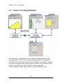
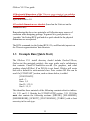
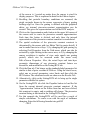
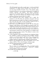
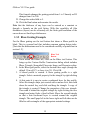
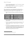

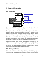
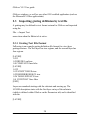


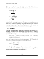
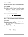
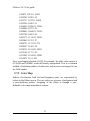
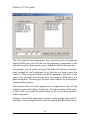
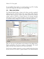

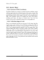
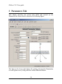


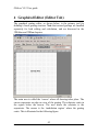
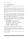

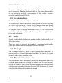

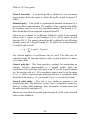
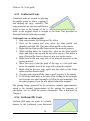
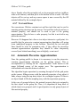
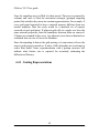
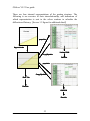

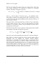
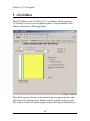
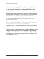
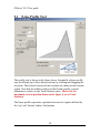
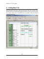
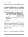
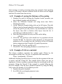
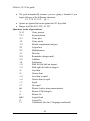
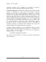

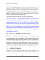
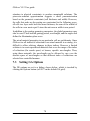
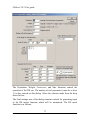


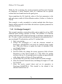
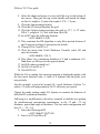

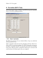
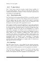
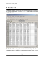
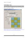
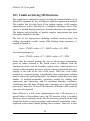
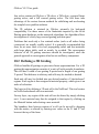


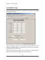
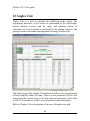


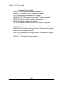


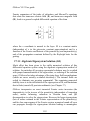

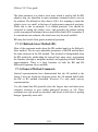
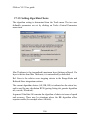
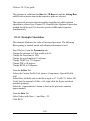
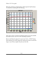
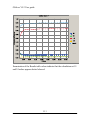

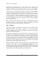
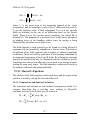
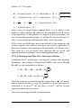
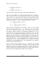
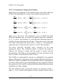


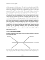
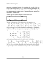
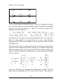
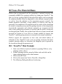
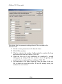


![or BTK [C481S] (cat. # CK-01-1002-384)](http://vs1.manualzilla.com/store/data/005787023_1-2d29b83e06663168d351d396f31f02d5-150x150.png)