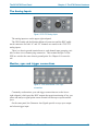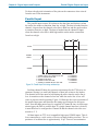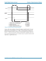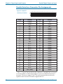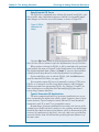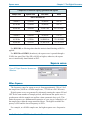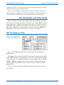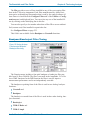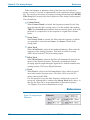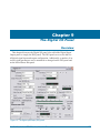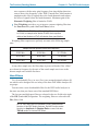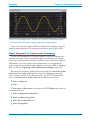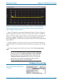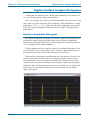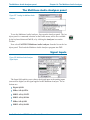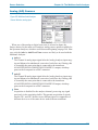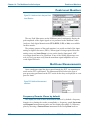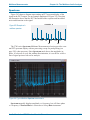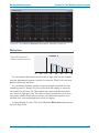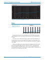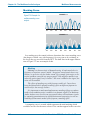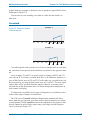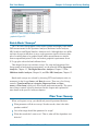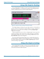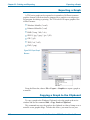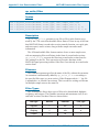
1
2700 Series User’s Manual for · SYS-2722 · and · SYS-2720 · · SYS-2712 · SYS-2702 · for version 3.1 control software Copyright Ó 2004 Audio Precision, Inc. All rights reserved. PN 8211.0183 Revision 1 For AP2700 control software Version 3.10 No part of this manual may be reproduced or transmitted in any form or by any means, electronic or mechanical, including photocopying, recording, or by any information storage and retrieval system, without permission in writing from the publisher. Audio Precision®, System One®, System Two™, System Two Cascade™, System Two Cascade Plus™, Cascade™, Cascade Plus™, System One + DSP™, System Two + DSP™, Dual Domain®, FASTTEST®, APWIN™, ATS™, ATS-2™, 2700 series™ and AP2700™ are trademarks of Audio Precision, Inc. Windows™ is a trademark of Microsoft Corporation. Audio Precision instruments equipped with the OPT-2711 Dolby™ Digital Generator are manufactured under license from Dolby Laboratories. Dolby and the double-D symbol are trademarks of Dolby Laboratories. Confidential unpublished works. © 1992–2004 Dolby Laboratories, Inc. All rights reserved. Published by: 5750 SW Arctic Drive Beaverton, Oregon 97005 Tel: 503-627-0832 Fax: 503-641-8906 US Toll Free: 1-800-231-7350 email: [email protected] Web: audioprecision.com Printed in the United States of America IV0409134647 Contents Safety Information . . . . . . . . . . . . . . . . . . . . . . . . . . . . . xxv Safety Symbols . . . . . . . . . . . . . . . . . . . . . . . . . . . . . . xxvi Chapter 1 Introduction . . . . . . . . . . . . . . . . . . . . . . . . . . . . . . . . . 1 The 2700 Series: an Overview. . . . . . . . . . . . . . . . . . . . . . . . 1 2700 Series Components . . . . . . . . . . . . . . . . . . . . . . . . . 2 2700 Series Instrument Models . . . . . . . . . . . . . . . . . . . . . . 3 About This Manual . . . . . . . . . . . . . . . . . . . . . . . . . . . . . . 4 Instruments supported. . . . . . . . . . . . . . . . . . . . . . . . . . . 4 SYS-2722 Capabilities . . . . . . . . . . . . . . . . . . . . . . . . . . . . 5 Architecture of 2700 Series Instruments . . . . . . . . . . . . . . . . . . . 7 Other Documentation for the 2700 series . . . . . . . . . . . . . . . . . . 7 Getting Started with the 2700 series. . . . . . . . . . . . . . . . . . . . 8 Online Help . . . . . . . . . . . . . . . . . . . . . . . . . . . . . . . . 8 The AP Basic Language Manual . . . . . . . . . . . . . . . . . . . . . 8 The AP Basic Extensions Reference for 2700 series . . . . . . . . . . . 9 The Filter Design Package Manual . . . . . . . . . . . . . . . . . . . . 9 Application Notes and TECHNOTES . . . . . . . . . . . . . . . . . . 10 Chapter 2 2700 Series Control Software . . . . . . . . . . . . . . . . . . . . . . 11 Overview . . . . . . . . The User Interface . . The Workspace. . . . . The 2700 series panels. Panel Settings . . . . Panel Readings . . . The 2700 series menus The File Menu . . . . The Edit Menu . . . . . . . . . . . . . . . . . . . . . . . . . . . . . . . . . . . . . . . . . . . . . . . . . . . . . . . . . . . . . . . . . . . . . . . . . . . . . . . . . . . . . . . . . . . . . . . . . . . . . . . . . . . . . . . . . . . . . . . . . . . . . . . . . . Audio Precision 2700 Series User’s Manual . . . . . . . . . . . . . . . . . . . . . . . . . . . . . . . . . . . . . . . . . . . . . . . . . . . . . . . . . . . . . . . . . . . . . . . . . . . . . . . . . . . . . . . . . . . . . . . . . . . . . . . . . . . . 11 11 12 12 13 14 15 15 16 i Contents The View Menu . . . . . . . . . . . . . . . . . . The Panels Menu . . . . . . . . . . . . . . . . . The Help Menu. . . . . . . . . . . . . . . . . . . Access to the Audio Precision Web site . . . . . The Status Bar . . . . . . . . . . . . . . . . . . . The Toolbars . . . . . . . . . . . . . . . . . . . . The Standard Toolbar . . . . . . . . . . . . . . The Panels Toolbar . . . . . . . . . . . . . . . The Macro Toolbar. . . . . . . . . . . . . . . . The Learn Mode Toolbar. . . . . . . . . . . . . The Quick Launch Toolbar . . . . . . . . . . . . Working with Files and AP2700 . . . . . . . . . . . Test Files . . . . . . . . . . . . . . . . . . . . . . System Two Cascade and Cascade Plus Tests . “New Test” files . . . . . . . . . . . . . . . . . Macro Files. . . . . . . . . . . . . . . . . . . . . Data Files . . . . . . . . . . . . . . . . . . . . . Waveform Files . . . . . . . . . . . . . . . . . . The Log File . . . . . . . . . . . . . . . . . . . . Keyboard Shortcuts . . . . . . . . . . . . . . . . . Function Keys . . . . . . . . . . . . . . . . . . . Other Keyboard Shortcuts . . . . . . . . . . . . . . . . . . . . . . . . . . . . . . . . . . . . . . . . . . . . . . . . . . . . . . . . . . . . . . . . . . . . . . . . . . . . . . . . . . . . . . . . . . . . . . . . . . . . . . . . . . . . . . . . . . . . . . . . . . . . . . . . . . . . . . . . . . . . . . . . . . . . . . . . . . . . . . . . . . . . . . . . . . . . . . . . . . . . . . . . . . . . . . . . . . . . . . . . . . . . . . . . . . . . . . . . . . . . . . . . . . . . . . . . . . . . . . . . . . . . . . . . . . . . . . . 17 18 20 21 21 21 22 23 25 25 25 26 26 27 27 27 27 28 29 29 29 31 Chapter 3 The 2700 Series Hardware . . . . . . . . . . . . . . . . . . . . . . . . 33 2700 Series Interface Bus . . . . . . . . . . . 2700 series Instrument Configurations . . . . . 2700 Series Major Options . . . . . . . . . . . 2700 Series Option Filters . . . . . . . . . . . Auxiliary Equipment for the 2700 Series . . . . The SYS-2722 Front Panel. . . . . . . . . . . Main Digital Input and Output . . . . . . . . The Analog Outputs . . . . . . . . . . . . . The Analog Inputs . . . . . . . . . . . . . . Monitor, sync and trigger connections . . . . The 2700 Series Rear Panel . . . . . . . . . . Labeling . . . . . . . . . . . . . . . . . . . Mains voltages and fusing . . . . . . . . . . Power Entry Module . . . . . . . . . . . . . The APIB interface connectors. . . . . . . . Sync, Reference and Auxiliary Connections . . . . . . . . . . . . . . . . . . . . . . . . . . . . . . . . . . . . . . . . . . . . . . . . . . . . . . . . . . . . . . . . . . . . . . . . . . . . . . . . . . . . . . . . . . . . . . . . . . . . . . . . . . . . . . . . . . . . . . . . . . . . . . . . . . . . . . . . . . . . . . . . . . . . . . . . . . . . . . . . . . . . . . . . . . . . . . . . . . . . . . . . . . . . . . . . . . . . . . . . . . . . . . . . . . . . . . . . . . . . . . . . . 33 33 34 35 35 37 37 38 39 39 40 40 40 41 41 42 Chapter 4 Signal Inputs and Outputs . . . . . . . . . . . . . . . . . . . . . . . . 45 The Analog Outputs . . . . . . . . . . . . . . . . . . . . . . . . . . . . 46 ii Audio Precision 2700 Series User’s Manual Contents Output Impedance . . . . . . . . . . . . . . . . . The Analog Inputs . . . . . . . . . . . . . . . . . . The Serial Digital Output . . . . . . . . . . . . . . . The Serial Digital Input . . . . . . . . . . . . . . . . Electrical vs. Data Characteristics Across Formats Parallel Digital Output and Input . . . . . . . . . . . Parallel Input . . . . . . . . . . . . . . . . . . . . Parallel Output . . . . . . . . . . . . . . . . . . . Parallel Interface Connector Pin Assignments . . . . . . . . . . . . . . . . . . . . . . . . . . . . . . . . . . . . . . . . . . . . . . . . . . . . . . . . . . . . . . . . . . . . . . . . . . . . . . . . . . . . . . . . . . . . . . . . . . . . . . 47 48 49 50 50 51 52 54 56 Chapter 5 Signal Analysis with the 2700 series . . . . . . . . . . . . . . . . . 57 Test Signal Generation in the 2700 series . . . . Two Audio Signal Generators . . . . . . . . . Analog Audio Signals. . . . . . . . . . . . . . . Analog Audio Generation and Output . . . . . The Analog Analyzer . . . . . . . . . . . . . . Digital Audio Signals . . . . . . . . . . . . . . . The Serial Digital Interface Signal . . . . . . . Digital Audio Generation . . . . . . . . . . . . The Digital Analyzer . . . . . . . . . . . . . . Real-Time and Batch Mode Measurements . The Digital Analyzer Analysis Tools . . . . . Sweeps and Graphs . . . . . . . . . . . . . . . . . . . . . . . . . . . . . . . . . . . . . . . . . . . . . . . . . . . . . . . . . . . . . . . . . . . . . . . . . . . . . . . . . . . . . . . . . . . . . . . . . . . . . . . . . . . . . . . . . . . . . . . . . . . . . . . . . . . . . . . . . . . . . . . . . . . . . . . . . . . . . . . . . . . . . . . . . . . 57 57 58 58 58 58 58 59 59 59 60 61 Chapter 6 The Analog Generator . . . . . . . . . . . . . . . . . . . . . . . . . . 63 Signals for Analog Measurements . . . . . . . . Signal generation in analog hardware . . . . Signal generation in DSP . . . . . . . . . . Performance Extremes versus Specifications . . The Analog Generator Panel . . . . . . . . . . . Frequency Units . . . . . . . . . . . . . . . . . Output ON/OFF and Channel Selection . . . . . Auto On . . . . . . . . . . . . . . . . . . . . Channel Invert . . . . . . . . . . . . . . . . . . Amplitude Control and Units . . . . . . . . . . . Choosing an Analog Generator Waveform . . . . Designation of hardware and DSP generation . Analog waveforms: speed versus accuracy . DSP waveforms: sample rate and bandwidth Sine waveforms . . . . . . . . . . . . . . . . Wfm: Sine: Normal. . . . . . . . . . . . . . Wfm: Sine: Burst. . . . . . . . . . . . . . . Wfm: Sine: Normal Burst . . . . . . . . . . . . . . . . . . . . . . . . . . . . Audio Precision 2700 Series User’s Manual . . . . . . . . . . . . . . . . . . . . . . . . . . . . . . . . . . . . . . . . . . . . . . . . . . . . . . . . . . . . . . . . . . . . . . . . . . . . . . . . . . . . . . . . . . . . . . . . . . . . . . . . . . . . . . . . . . . . . . . . . . . . . . . . . . . . . . . . . . . . . . . . . . . . . . . . . . . . . . . . . . . . . . . . . . . . . . . . . . . . . . . . . . . . . . . . . . . . . . . . . . . . . . . . . . . . . . . . 63 64 64 65 66 67 67 67 68 68 69 69 69 70 70 70 71 71 iii Contents Wfm: Sine: Gated Burst . . . . . . . . . . . Wfm: Sine: Trig. Burst . . . . . . . . . . . . Wfm: Sine: EQ Sine . . . . . . . . . . . . . Sine waveforms from DSP . . . . . . . . . . . Wfm: Sine (D/A): Var Phase . . . . . . . . . Wfm: Sine (D/A): Stereo . . . . . . . . . . . Wfm: Sine (D/A): Dual . . . . . . . . . . . . Wfm: Sine (D/A): Shaped Burst . . . . . . . Wfm: Sine (D/A): EQ Sine . . . . . . . . . . Square wave waveforms . . . . . . . . . . . . Wfm: Square. . . . . . . . . . . . . . . . . Wfm: Square (D/A) . . . . . . . . . . . . . Intermodulation Distortion (IMD) waveforms . . Wfm: IMD: SMPTE/DIN 1:1 . . . . . . . . . Wfm: IMD: SMPTE/DIN 4:1 . . . . . . . . . Wfm: IMD: CCIF/DFD . . . . . . . . . . . . Wfm: IMD: DIM 30 / DIM 100 / DIM B . . . . Wfm: IMD (D/A): SMPTE/DIN 1:1 . . . . . . Wfm: IMD (D/A): SMPTE/DIN 4:1 . . . . . . Wfm: IMD (D/A): CCIF/DFD . . . . . . . . . Wfm: IMD (D/A): DIM 30 / DIM 100 / DIM B . Noise Waveforms . . . . . . . . . . . . . . . Random vs. Pseudo-random . . . . . . . . Noise amplitude calibration . . . . . . . . . Wfm: Noise: Pseudo . . . . . . . . . . . . . Wfm: Noise: Random . . . . . . . . . . . . Variable Bandpass Filter for Pink Noise . . . Wfm: Noise (D/A) . . . . . . . . . . . . . . Arbitrary Waveforms . . . . . . . . . . . . . . Wfm: Arb Wfm (D/A) . . . . . . . . . . . . . Arbitrary Waveforms and D/A Sample Rate . . MLS Waveforms . . . . . . . . . . . . . . . . Wfm: MLS (D/A) . . . . . . . . . . . . . . . MLS Waveform Sample Rate . . . . . . . . . Special Waveforms. . . . . . . . . . . . . . . Wfm: Special (D/A): Polarity . . . . . . . . . Wfm: Special (D/A): Pass Thru . . . . . . . Setting the D/A Bandwidth . . . . . . . . . . . Setting the D/A Sample Rate. . . . . . . . . . Configuring the Analog Outputs . . . . . . . . . Analog Generator References . . . . . . . . . . dBm Reference . . . . . . . . . . . . . . . . dBr Reference . . . . . . . . . . . . . . . . . Frequency Reference . . . . . . . . . . . . . iv . . . . . . . . . . . . . . . . . . . . . . . . . . . . . . . . . . . . . . . . . . . . . . . . . . . . . . . . . . . . . . . . . . . . . . . . . . . . . . . . . . . . . . . . . . . . . . . . . . . . . . . . . . . . . . . . . . . . . . . . . . . . . . . . . . . . . . . . . . . . . . . . . . . . . . . . . . . . . . . . . . . . . . . . . . . . . . . . . . . . . . . . . . . . . . . . . . . . . . . . . . . . . . . . . . . . . . . . . . . . . . . . . . . . . . . . . . . . . . . . . . . . . . . . . . . . . . . . . . . . . . . . . . . . . . . . . . . . . . . . . . . . . . . . . . . . . . . . . . . . . . . . . . . . . . . . . . . . . . . . . . . . . . . . . . . . . . . . . . . . . . . . . . . . . . . . . . . . . . . . . . . . . . . . . . . . . . . . . . . . . . . . . . . . . . . . . . . . . . . . . . . . . . . . . . . . . . . . . . . . . . . . . . . . . . . . . . . . . . . . . . . . . . . . . . . . . . . . . . . . . . . . . . . . . . . . . . . . . . . . . . . . . . . . . . . . . . . . . . . . . . . . . . . . . . . . . . . . . . . . . . . . . . . . . . . . . . . . . . . . . . . . . . . . . . . . . . . . . . . . . . . . . . . . . . . . 72 72 74 75 75 77 78 78 79 80 80 80 81 81 82 82 83 83 84 84 85 85 86 86 87 88 88 89 90 90 90 91 91 91 92 92 92 94 94 95 96 97 97 97 Audio Precision 2700 Series User’s Manual Contents Watts Reference . . . . . . . . . . . . . . . . . . . . . . . . . . . . . 97 Chapter 7 The Digital Generator . . . . . . . . . . . . . . . . . . . . . . . . . . . 99 Signals for Digital Measurements. . . . . . . . . . . . . . . . . . . . . . 99 The Digital Generator Panel . . . . . . . . . . . . . . . . . . . . . . . . 99 Frequency Units . . . . . . . . . . . . . . . . . . . . . . . . . . . . . . 100 Output On/Off and Channel Selection. . . . . . . . . . . . . . . . . . . 100 Auto On . . . . . . . . . . . . . . . . . . . . . . . . . . . . . . . . . 101 Channel Invert. . . . . . . . . . . . . . . . . . . . . . . . . . . . . . . 101 Amplitude Control and Units . . . . . . . . . . . . . . . . . . . . . . . 101 Choosing a Digital Generator Waveform . . . . . . . . . . . . . . . . . 102 Sine waveforms . . . . . . . . . . . . . . . . . . . . . . . . . . . . . . 103 Wfm: Sine: Normal . . . . . . . . . . . . . . . . . . . . . . . . . . . 103 Wfm: Sine: Burst . . . . . . . . . . . . . . . . . . . . . . . . . . . . 103 Wfm: Sine: Var Phase . . . . . . . . . . . . . . . . . . . . . . . . . 104 Wfm: Sine: Stereo . . . . . . . . . . . . . . . . . . . . . . . . . . . 105 Wfm: Sine: Dual . . . . . . . . . . . . . . . . . . . . . . . . . . . . 105 Wfm: Sine+Offset . . . . . . . . . . . . . . . . . . . . . . . . . . . . 106 Wfm: Sine: EQ . . . . . . . . . . . . . . . . . . . . . . . . . . . . . 106 Wfm: Sine: Shaped Burst . . . . . . . . . . . . . . . . . . . . . . . . 107 Intermodulation Distortion (IMD) . . . . . . . . . . . . . . . . . . . . . 108 Wfm: IMD: SMPTE/DIN 1:1 . . . . . . . . . . . . . . . . . . . . . . . 109 Wfm: IMD: SMPTE/DIN 4:1 . . . . . . . . . . . . . . . . . . . . . . . 109 Wfm: IMD: CCIF/DFD. . . . . . . . . . . . . . . . . . . . . . . . . . 109 Wfm: IMD: DIM 30 / DIM 100 / DIM B. . . . . . . . . . . . . . . . . . 110 Square wave. . . . . . . . . . . . . . . . . . . . . . . . . . . . . . . . 111 Wfm: Square . . . . . . . . . . . . . . . . . . . . . . . . . . . . . . 111 Noise . . . . . . . . . . . . . . . . . . . . . . . . . . . . . . . . . . . 112 Wfm: Noise: White . . . . . . . . . . . . . . . . . . . . . . . . . . . 112 Wfm: Noise: Pink . . . . . . . . . . . . . . . . . . . . . . . . . . . . 112 Wfm: Noise: Burst USASI . . . . . . . . . . . . . . . . . . . . . . . . 113 Special Waveforms . . . . . . . . . . . . . . . . . . . . . . . . . . . . 113 Wfm: Special: Monotonicity . . . . . . . . . . . . . . . . . . . . . . . 113 Wfm: Special: J-Test . . . . . . . . . . . . . . . . . . . . . . . . . . 114 Wfm: Special: Polarity. . . . . . . . . . . . . . . . . . . . . . . . . . 115 Wfm: Special: Walking Ones and Walking Zeros . . . . . . . . . . . . 116 Wfm: Special: Constant Value. . . . . . . . . . . . . . . . . . . . . . 116 Wfm: Special: Random . . . . . . . . . . . . . . . . . . . . . . . . . 117 Wfm: Special: Pass Thru . . . . . . . . . . . . . . . . . . . . . . . . 117 MLS Waveforms. . . . . . . . . . . . . . . . . . . . . . . . . . . . . . 118 Wfm: MLS. . . . . . . . . . . . . . . . . . . . . . . . . . . . . . . . 118 MLS Waveform Sample Rate . . . . . . . . . . . . . . . . . . . . . . 118 Arbitrary Waveforms. . . . . . . . . . . . . . . . . . . . . . . . . . . . 119 Audio Precision 2700 Series User’s Manual v Contents Dither . . . . . . . . . . . . . . Dither Type . . . . . . . . . . Digital Generator References . . Volts for Full Scale Reference Frequency Reference. . . . . dBr Reference . . . . . . . . . . . . . . . . . . . . . . . . . . . . . . . . . . . . . . . . . . . . . . . . . . . . . . . . . . . . . . . . . . . . . . . . . . . . . . . . . . . . . . . . . . . . . . . . . . . . . . . . . . . . . . . . . . . . . . . . . . . . . . . . . . . . . . 120 120 121 122 122 122 Chapter 8 The Analog Analyzer . . . . . . . . . . . . . . . . . . . . . . . . . . 123 Overview . . . . . . . . . . . . . . . . . Analog Analyzer Options . . . . . . . . The Analog Analyzer Panel . . . . . . . . Input Selection and Configuration . . . . . Source Input Termination . . . . . . . . DC Coupling of Analog Inputs . . . . . The Level Meters . . . . . . . . . . . . . Level Meter Units . . . . . . . . . . . . The Frequency Meters . . . . . . . . . . Input Ranging . . . . . . . . . . . . . . . Autoranging . . . . . . . . . . . . . . . Fixed Range . . . . . . . . . . . . . . The Phase Meter . . . . . . . . . . . . . Phase Meter Hardware . . . . . . . . . The Function Meter . . . . . . . . . . . . Function Meter Units . . . . . . . . . . Function Meter Ranging . . . . . . . . Function Meter Channel Selection . . . Function Meter Measurement Functions Amplitude . . . . . . . . . . . . . . . . Bandpass . . . . . . . . . . . . . . . Bandreject . . . . . . . . . . . . . . . THD+N Ampl . . . . . . . . . . . . . . THD+N Ratio . . . . . . . . . . . . . . IMD Measurements: SMPTE/DIN . . . IMD Measurements: CCIF and DFD. . CCIF . . . . . . . . . . . . . . . . . DFD . . . . . . . . . . . . . . . . . IMD Measurements: DIM (TIM) . . . . Wow and Flutter Measurements . . . . Ranging Considerations . . . . . . . FM discriminator . . . . . . . . . . . Weighting and Bandpass Filters . . . Detector Selection . . . . . . . . . . 2-Ch. Ratio . . . . . . . . . . . . . . . vi . . . . . . . . . . . . . . . . . . . . . . . . . . . . . . . . . . . . . . . . . . . . . . . . . . . . . . . . . . . . . . . . . . . . . . . . . . . . . . . . . . . . . . . . . . . . . . . . . . . . . . . . . . . . . . . . . . . . . . . . . . . . . . . . . . . . . . . . . . . . . . . . . . . . . . . . . . . . . . . . . . . . . . . . . . . . . . . . . . . . . . . . . . . . . . . . . . . . . . . . . . . . . . . . . . . . . . . . . . . . . . . . . . . . . . . . . . . . . . . . . . . . . . . . . . . . . . . . . . . . . . . . . . . . . . . . . . . . . . . . . . . . . . . . . . . . . . . . . . . . . . . . . . . . . . . . . . . . . . . . . . . . . . . . . . . . . . . . . . . . . . . . . . . . . . . . . . . . . . . . . . . . . . . . . . . . . . . . . . . . . . . . . . . . . . . . . . . . . . . . . . . . . . . . . . . . . . . . . . . . . . . . . . . . . . . . . . . . . . . . . . . . . . . . . . . . . . . . . . . . . . . . . . . . . . . . . . . . . . . . . . . . . . . . . . . . . . . . . . . . . . . . . . . . . . . . . . . . . . . . . . . . . . . . . . . . . . . . . . . . . . . . . . . . . . . . . . . . . . . . 123 124 126 126 127 127 128 128 129 130 130 130 131 132 132 132 133 133 133 134 135 135 136 137 137 138 138 139 139 140 141 141 141 142 143 Audio Precision 2700 Series User’s Manual Contents Crosstalk . . . . . . . . . . . . . . Detector Type . . . . . . . . . . . . Detector Reading Rate . . . . . . . The Bandwidth and Filter Fields. . . . BW: The Highpass Filter . . . . . . BW: The Lowpass Filter . . . . . . The “Fltr” Field . . . . . . . . . . Bandpass/Bandreject Filter Tuning . References . . . . . . . . . . . . . . . . . . . . . . . . . . . . . . . . . . . . . . . . . . . . . . . . . . . . . . . . . . . . . . . . . . . . . . . . . . . . . . . . . . . . . . . . . . . . . . . . . . . . . . . . . . . . . . . . . . . . . . . . . . . . . . . . . . . . . . . . . . . . . . . . . . . . . . . . . . . . . . . . . . . . . . . . . . . . . . . . 143 144 146 147 147 148 148 149 150 Chapter 9 The Digital I/O Panel . . . . . . . . . . . . . . . . . . . . . . . . . . . 153 Overview . . . . . . . . . . . . . . . . The DIO Output Section. . . . . . . . . Connector. . . . . . . . . . . . . . . SR Range. . . . . . . . . . . . . . . Sample Rate (SR) . . . . . . . . . . System Sample Rate (SSR) . . . . . Voltage . . . . . . . . . . . . . . . . Output Audio Format . . . . . . . . . Linear . . . . . . . . . . . . . . . . . µ-Law and A-law Compression . . . . IEC 61937 (Dolby Digital) . . . . . . . Preemphasis . . . . . . . . . . . . . Scale Freq. by . . . . . . . . . . . . Output Impairments . . . . . . . . . . . The Output Impairment Checkboxes . Invert . . . . . . . . . . . . . . . . Cable Simulation . . . . . . . . . . Changing the Parity bit . . . . . . . Sending a high Validity bit . . . . . Rise/Fall Time . . . . . . . . . . . Interfering Noise . . . . . . . . . . Common Mode Sine . . . . . . . . Jitter Generation . . . . . . . . . . . Jitter Type . . . . . . . . . . . . . Amplitude. . . . . . . . . . . . . . Frequency . . . . . . . . . . . . . EQ Curve . . . . . . . . . . . . . . The DIO Input Section . . . . . . . . . Connector. . . . . . . . . . . . . . . Input Impedance . . . . . . . . . . . Connector I & II Selection. . . . . . . Normal Operation . . . . . . . . . . . . . . . . . . . . . . . . . . . . . . . . . . . . . . . . . . . . . . . . . . . . . . . . . . . . . . . . . . . . . . . . . . . . . . . . . . . . . . . . . . . . . . . . . . . . . . . . . . . . . . . . . . . . . . . . . . . . . . . . . . . . . . . . . . . . . . . . . . . . . . . . . . . . . . . . . . . . . . . . . . . . . . . . . . . . . . . . . . . . . . . . . . . . . . . . . Audio Precision 2700 Series User’s Manual . . . . . . . . . . . . . . . . . . . . . . . . . . . . . . . . . . . . . . . . . . . . . . . . . . . . . . . . . . . . . . . . . . . . . . . . . . . . . . . . . . . . . . . . . . . . . . . . . . . . . . . . . . . . . . . . . . . . . . . . . . . . . . . . . . . . . . . . . . . . . . . . . . . . . . . . . . . . . . . . . . . . . . . . . . . . . . . . . . . . . . . . . . . . . . . . . . . . . . . . . . . . . . . . . . . . . . . . . . . . . . . . . . . . . . . . . . . . . . . . . . . . . . . . . . . . . . . . . . . . . . . . . . . . . . . . . . . . . . . . . . . . . . . . . . . . . . . . . . . . . . . . . . . . . . . . . . . . . . . . . . . . . . . . . . . . . . . . . . . . . . . . . . . . . . . . 153 154 155 156 157 157 158 159 159 160 160 161 161 162 162 162 162 163 164 164 164 164 165 165 166 167 167 168 169 170 171 171 vii Contents Dual Connector Operation . . . . . . Sample Rate-ISR . . . . . . . . . . . . Voltage . . . . . . . . . . . . . . . . . Input Audio Format . . . . . . . . . . . Linear . . . . . . . . . . . . . . . . . . µ-Law and A-law Expansion . . . . . . Deemphasis . . . . . . . . . . . . . . Scale Freq. by . . . . . . . . . . . . . Delay from Ref Out . . . . . . . . . . . Rate Ref . . . . . . . . . . . . . . . . Peak Monitors . . . . . . . . . . . . . Data Bit Indicators . . . . . . . . . . . Error Indicators . . . . . . . . . . . . . The Confidence Indicator. . . . . . . The Lock Indicator . . . . . . . . . . The Coding Indicator . . . . . . . . . The Parity Bit Indicator . . . . . . . . The Validity Bit Indicators. . . . . . . Jitter Measurement . . . . . . . . . . . The Status Bits panel . . . . . . . . . . . Transmit Status Bits. . . . . . . . . . . Consumer Format Status Bits . . . . Professional Format Status Bits . . . Local Address and Time of Day entry CRC entry . . . . . . . . . . . . . . Receive Status Bits . . . . . . . . . . . Hex Control and Display . . . . . . . . Dual Connector Mode and Status Bits . . . . . . . . . . . . . . . . . . . . . . . . . . . . . . . . . . . . . . . . . . . . . . . . . . . . . . . . . . . . . . . . . . . . . . . . . . . . . . . . . . . . . . . . . . . . . . . . . . . . . . . . . . . . . . . . . . . . . . . . . . . . . . . . . . . . . . . . . . . . . . . . . . . . . . . . . . . . . . . . . . . . . . . . . . . . . . . . . . . . . . . . . . . . . . . . . . . . . . . . . . . . . . . . . . . . . . . . . . . . . . . . . . . . . . . . . . . . . . . . . . . . . . . . . . . . . . . . . . . . . . . . . . . . . . . . . . . . . . . . . . . . . . . . . . . . . . . . . . . . . . . . . . . . . . . . . . . . . . . . . . . . . . . . . . . . . . . . . . . . . . . . . . . . . . . . . . . . . . . . . . . . . . . . . . . . . . . . . . . . . . . . . . . . . . . . . . . . . . . . . . . . . . . . . . . . . . . . . . . . . . . . . . . . . . . . . . . . . . . . . . . . . . . . . 171 171 172 172 173 173 174 174 175 176 176 177 177 178 178 178 178 179 179 180 181 182 183 183 184 184 185 185 Chapter 10 The Dolby Digital Generator . . . . . . . . . . . . . . . . . . . . . . 187 Overview . . . . . . . . . . . . . . . . . . . . . . . . Connections . . . . . . . . . . . . . . . . . . . . . . . Using the Dolby Digital Generator. . . . . . . . . . . . Data-type . . . . . . . . . . . . . . . . . . . . . . . Levels of control . . . . . . . . . . . . . . . . . . . Dolby Digital at Normal Level of Control . . . . . . . Dolby Digital at Advanced or Expert Levels of Control Channel Routing to the Dolby Digital inputs . . . . . Normal . . . . . . . . . . . . . . . . . . . . . . . Follow Switcher. . . . . . . . . . . . . . . . . . . Dolby Digital controls . . . . . . . . . . . . . . . . . . Audio Service Configuration . . . . . . . . . . . . . frmsizecod . . . . . . . . . . . . . . . . . . . . . viii . . . . . . . . . . . . . . . . . . . . . . . . . . . . . . . . . . . . . . . . . . . . . . . . . . . . . . . . . . . . . . . . . . . . . . . . . . . . . . . . . . . . . . . . . . . . . . . . . . . . . . . . . . . . . . . . . . . . . 187 188 188 189 191 192 193 193 194 194 195 195 195 Audio Precision 2700 Series User’s Manual Contents fscod mode . . . . . . . . . . fscod . . . . . . . . . . . . . acmod . . . . . . . . . . . . lfeon . . . . . . . . . . . . . bsmod . . . . . . . . . . . . dialnorm . . . . . . . . . . . dialnorm2 . . . . . . . . . . . Bitstream information . . . . . . cmixlev . . . . . . . . . . . . surmixlev . . . . . . . . . . . dsurmod . . . . . . . . . . . copyrightb . . . . . . . . . . origbs. . . . . . . . . . . . . audprodie. . . . . . . . . . . mixlevel. . . . . . . . . . . . roomtyp. . . . . . . . . . . . audprodi2e . . . . . . . . . . mixlevel2 . . . . . . . . . . . roomtyp2 . . . . . . . . . . . langcode . . . . . . . . . . . langcod . . . . . . . . . . . . langcod2e . . . . . . . . . . langcod2 . . . . . . . . . . . Extended Bitstream information Extended bitstream . . . . . . bsid mode . . . . . . . . . . bsid . . . . . . . . . . . . . . xbsi1e . . . . . . . . . . . . dmixmod . . . . . . . . . . . lorocmixlev . . . . . . . . . . lorosurmixlev . . . . . . . . . ltrtcmixlev. . . . . . . . . . . ltrtsurmixlev. . . . . . . . . . xbsi2e . . . . . . . . . . . . dsurexmod . . . . . . . . . . dheadphonmod. . . . . . . . adconvtyp . . . . . . . . . . xbsi2 . . . . . . . . . . . . . encinfo . . . . . . . . . . . . Time Code . . . . . . . . . . . timecod1e . . . . . . . . . . timecod2e . . . . . . . . . . Preprocessing . . . . . . . . . Channel Lowpass . . . . . . . . . . . . . . . . . . . . . . . . . . . . . . . . . . . . . . . . . . . . . . . . . . . . . . . . . . . . . . . . . . . . . . . . . . . . . . . . . . . . . . . . . . . . . . . . . . . . . . . . . . . . . . . . . . . . . . . . . . . . . . . . . . . . . . . . . . . . . . . . . . . . . . . . . . . . . . . . . . . . . . . . . . . . . . . . . . . . . . . . . . . . . . . . . . . . . . . . . . . . . . . . . . . . . . . . . . . . . . . . . . . . . . . . . . . . . . . . . . . . . . . . . . . . . . . . . . . . . . . . . . . . . . . . . . . . . . . . . . . . . . . . . . . . . . . . . . . . . . . . . . . . . . . . . . . . . . . . . . . . . . . . . . . . . . . . . . . . . . . . . . . . . . . . . . . . . . . . . . . . . . . . . . . . . . . . . . . . . . . . . . . . . . . . . . . . . . . . . . Audio Precision 2700 Series User’s Manual . . . . . . . . . . . . . . . . . . . . . . . . . . . . . . . . . . . . . . . . . . . . . . . . . . . . . . . . . . . . . . . . . . . . . . . . . . . . . . . . . . . . . . . . . . . . . . . . . . . . . . . . . . . . . . . . . . . . . . . . . . . . . . . . . . . . . . . . . . . . . . . . . . . . . . . . . . . . . . . . . . . . . . . . . . . . . . . . . . . . . . . . . . . . . . . . . . . . . . . . . . . . . . . . . . . . . . . . . . . . . . . . . . . . . . . . . . . . . . . . . . . . . . . . . . . . . . . . . . . . . . . . . . . . . . . . . . . . . . . . . . . . . . . . . . . . . . . . . . . . . . . . . . . . . . . . . . . . . . . . . . . . . . . . . . . . . . . . . . . . . . . . . . . . . . . . . . . . . . . . . . . . . . . . . . . . . . . . . . . . . . . . . . . . . . . . . . . . . . . . . . . . . . . . . . . . . . . . . . . . . . . . . . . . . . . . . . . . . . . . . . . . . . . . . . . . . . . . . . . . . . . . . . . . . . . . . . . . . . . . . . . . 196 196 197 197 197 198 198 198 199 199 199 200 200 200 200 200 201 201 201 201 201 202 202 202 202 203 203 204 204 204 205 205 206 206 206 207 207 207 208 208 208 208 208 208 ix Contents DC Highpass . . . . . . . . . . . . . . . . . LFE Lowpass . . . . . . . . . . . . . . . . . Phase Shift . . . . . . . . . . . . . . . . . . Dynamic Range Compression . . . . . . . . . Line mode compression . . . . . . . . . . . dynrng . . . . . . . . . . . . . . . . . . . . RF mode compression . . . . . . . . . . . . compr . . . . . . . . . . . . . . . . . . . . . Impairments. . . . . . . . . . . . . . . . . . . crc1. . . . . . . . . . . . . . . . . . . . . . crc2. . . . . . . . . . . . . . . . . . . . . . syncword . . . . . . . . . . . . . . . . . . . syncword mode. . . . . . . . . . . . . . . . IEC 61937 bitstream and controls. . . . . . . . . Levels of Control . . . . . . . . . . . . . . . IEC 61937 Idle Data-type (Null data-bursts) . . Send Null Data-Bursts . . . . . . . . . . . . Null data-burst repetition period . . . . . . . Pause Data-type . . . . . . . . . . . . . . . . Pause data-burst repetition. . . . . . . . . . (Pause) Data-burst repetition mode . . . . . (Pause) data-burst repetition period . . . . . gap-length mode and gap-length . . . . . . . Preambles controls . . . . . . . . . . . . . . . . Data-type mode. . . . . . . . . . . . . . . . . Data-type (preambles) . . . . . . . . . . . . . Data-type code . . . . . . . . . . . . . . . . . Reserved bits . . . . . . . . . . . . . . . . . . Error flag . . . . . . . . . . . . . . . . . . . . Data-type-dependent info mode . . . . . . . . Data-type-dependent info . . . . . . . . . . . . Bitstream number mode . . . . . . . . . . . . Bitstream number . . . . . . . . . . . . . . . . Length-code mode . . . . . . . . . . . . . . . Length-code . . . . . . . . . . . . . . . . . . Sweepable parameters . . . . . . . . . . . . . . Sweep settling and IEC 61937 processing . . . . OPT-2711 Required Components . . . . . . . . . APSI: the Audio Precision Streaming Interface . OPT-2711 Licensing . . . . . . . . . . . . . . References . . . . . . . . . . . . . . . . . . . . . . . . . . . . . . . . . . . . . . . . . . . . . . . . . . . . . . . . . . . . . . . . . . . . . . . . . . . . . . . . . . . . . . . . . . . . . . . . . . . . . . . . . . . . . . . . . . . . . . . . . . . . . . . . . . . . . . . . . . . . . . . . . . . . . . . . . . . . . . . . . . . . . . . . . . . . . . . . . . . . . . . . . . . . . . . . . . . . . . . . . . . . . . . . . . . . . . . . . . . . . . . . . . . . . . . . . . . . . . . . . . . . . . . . . . . . . . . . . . . . . . . . . . . . . . . . . . . . . . . . . . . . . . . . . . . . . . . . . . . . . . . . . . . . . . . . . . . . . . . . . . . . . . . . . . . . . . . . . . . . . . . . . . . . . . . . . . . . . . . . . . . . . . . . . . . . . . . . . . . . . . . . . . . . . . . . . . . . . . . . . . . . . . . . . . . . . . . . . . . . . . . . . . . . . . . . . . . . . . . . . . . . . . . . . . . . . . . . . . . . . . . . . . . . . . . . . . . . . . . . . . . . . . . . . . . . . . . . . . . . . . . . . . . . . . . . 209 209 209 209 209 210 211 211 212 212 212 213 213 213 214 214 215 215 215 216 217 217 217 218 218 219 220 220 220 220 220 221 221 221 221 222 222 222 222 223 224 Chapter 11 The DSP Audio Analyzer . . . . . . . . . . . . . . . . . . . . . . . . 225 x Audio Precision 2700 Series User’s Manual Contents Overview . . . . . . . . . . . . . . . . . . . . . Loading the DSP Audio Analyzer . . . . . . . . . Signal Inputs . . . . . . . . . . . . . . . . . . . Digital @ISR . . . . . . . . . . . . . . . . . . HiRes A/D & HiBW A/D . . . . . . . . . . . . . Converter and Sample Rate Selection . . . . . Source . . . . . . . . . . . . . . . . . . . . . . Coupling. . . . . . . . . . . . . . . . . . . . . . The Level Meters . . . . . . . . . . . . . . . . . Level Meter Units . . . . . . . . . . . . . . . . The Frequency Meters . . . . . . . . . . . . . . Meter Ranging . . . . . . . . . . . . . . . . . . Autoranging . . . . . . . . . . . . . . . . . . . Fixed Range . . . . . . . . . . . . . . . . . . The Function (Reading) Meters . . . . . . . . . . Function Meter Measurement Functions . . . . Amplitude Function . . . . . . . . . . . . . . 2-Channel Ratio Function . . . . . . . . . . Crosstalk Function . . . . . . . . . . . . . . THD+N Ratio and Amplitude Functions . . . Bandpass Function . . . . . . . . . . . . . . SMPTE / DIN IMD Function . . . . . . . . . Phase Function. . . . . . . . . . . . . . . . Function Meter Units . . . . . . . . . . . . . . Function Meter Ranging . . . . . . . . . . . . Detector Type . . . . . . . . . . . . . . . . . . Detector Reading Rate . . . . . . . . . . . . . The Bandwidth and Filter Fields . . . . . . . . BW: The Highpass Filter . . . . . . . . . . . BW: The Lowpass Filter . . . . . . . . . . . The “Fltr” Field . . . . . . . . . . . . . . . . Fltr: Weighting Filters . . . . . . . . . . . . . User Filters . . . . . . . . . . . . . . . . . . Bandpass/Bandreject Filter Tuning . . . . . . Fltr: Selecting Harmonics in Bandpass . . . . References . . . . . . . . . . . . . . . . . . . . Digital Analyzer References . . . . . . . . . . Analog References for the DSP Audio Analyzer . . . . . . . . . . . . . . . . . . . . . . . . . . . . . . . . . . . . . . . . . . . . . . . . . . . . . . . . . . . . . . . . . . . . . . . . . . . . . . . . . . . . . . . . . . . . . . . . . . . . . . . . . . . . . . . . . . . . . . . . . . . . . . . . . . . . . . . . . . . . . . . . . . . . . . . . . . . . . . . . . . . . . . . . . . . . . . . . . . . . . . . . . . . . . . . . . . . . . . . . . . . . . . . . . . . . . . . . . . . . . . . . . . . . . . . . . . . . . . . . . . . . . . . . . . . . . . . . . . . . . . . . . . . . . . . . . . . . . . . . . . . . . . . . . . . . . . . . . . . . . . . . . . . . . . . . . . . . . . . . . . . . . . . . . . . . . . . . . . . . . . . . . . . . . . . . . . . . . . . . . . . . . . . . . . . . . . . . . . . . . . . . . . . . . . . . . . . . . . . . . . . . . . . . . . . . . . . . . . . . . . . . . . . . . . . . . . . . . . . . . . . . . . . . . . . . . . . . 225 227 228 228 228 229 230 230 231 231 232 233 233 233 234 234 235 237 239 241 243 245 247 248 249 249 251 251 252 252 253 253 255 257 259 259 259 260 Chapter 12 The Spectrum Analyzer . . . . . . . . . . . . . . . . . . . . . . . . . 261 Introduction . . . . . . . . . . . . . . . . . . . . . . . . . . . . . . . . 261 Loading the Spectrum Analyzer . . . . . . . . . . . . . . . . . . . . . . 262 Signal Inputs . . . . . . . . . . . . . . . . . . . . . . . . . . . . . . . 262 Audio Precision 2700 Series User’s Manual xi Contents Source Selection . . . . . . . . . . . . . . . . . . . . . . Digital @ISR Sources. . . . . . . . . . . . . . . . . . . Analog (A/D) Sources. . . . . . . . . . . . . . . . . . . Peak Level Monitors . . . . . . . . . . . . . . . . . . . . Acquiring, Transforming and Processing . . . . . . . . . . The Acquisition Record . . . . . . . . . . . . . . . . . . . Acquisition Length. . . . . . . . . . . . . . . . . . . . . . FFT Length . . . . . . . . . . . . . . . . . . . . . . . . . FFT Window Selection . . . . . . . . . . . . . . . . . . . Hann Window . . . . . . . . . . . . . . . . . . . . . . . Blackman-Harris Window . . . . . . . . . . . . . . . . . Flat-Top Window . . . . . . . . . . . . . . . . . . . . . Equiripple Window . . . . . . . . . . . . . . . . . . . . Hamming Window . . . . . . . . . . . . . . . . . . . . Gaussian Window. . . . . . . . . . . . . . . . . . . . . Rife-Vincent Windows . . . . . . . . . . . . . . . . . . None (No Window or Rectangular Window) . . . . . . . None, move to bin center . . . . . . . . . . . . . . . . . Quasi-AC Coupling . . . . . . . . . . . . . . . . . . . . . Averaging . . . . . . . . . . . . . . . . . . . . . . . . . . Synchronous Averaging . . . . . . . . . . . . . . . . . Signal Alignment for Synchronous Averaging . . . . . Sync (without re-align) . . . . . . . . . . . . . . . . . Sync, re-align. . . . . . . . . . . . . . . . . . . . . . Synchronous Averaging for “Move to bin center” . . . . Synchronous Averaging and Frequency Domain Views Power (Spectrum) Averaging . . . . . . . . . . . . . . . Display Processing . . . . . . . . . . . . . . . . . . . . . Waveform (time domain) Display Processing. . . . . . . Interpolate . . . . . . . . . . . . . . . . . . . . . . . Display Samples . . . . . . . . . . . . . . . . . . . . Peak Values . . . . . . . . . . . . . . . . . . . . . . Absolute Values . . . . . . . . . . . . . . . . . . . . Graphic Aliasing . . . . . . . . . . . . . . . . . . . . . Spectrum (frequency domain) Display Processing . . . . Octave Smoothing . . . . . . . . . . . . . . . . . . . Peak Picking . . . . . . . . . . . . . . . . . . . . . . FFT Start Time . . . . . . . . . . . . . . . . . . . . . . . Triggering . . . . . . . . . . . . . . . . . . . . . . . . . . Free Run . . . . . . . . . . . . . . . . . . . . . . . . . Auto. . . . . . . . . . . . . . . . . . . . . . . . . . . . Fixed Sensitivity . . . . . . . . . . . . . . . . . . . . . Trig In (Ext) . . . . . . . . . . . . . . . . . . . . . . . . Digital Gen . . . . . . . . . . . . . . . . . . . . . . . . xii . . . . . . . . . . . . . . . . . . . . . . . . . . . . . . . . . . . . . . . . . . . . . . . . . . . . . . . . . . . . . . . . . . . . . . . . . . . . . . . . . . . . . . . . . . . . . . . . . . . . . . . . . . . . . . . . . . . . . . . . . . . . . . . . . . . . . . . . . . . . . . . . . . . . . . . . . . . . . . . . . . . . . . . . . . . . . . . . . . . . . . . . . . . . . . . . . . . . . . . . . . . . . . . . . . . . . . . . . . . . . . . . . . . . . . . . . . . . . . . . . . . . . . . . . . . . . . . . . . . . . . . . . . . . . . . . . . . . . . . . . . . . . . . . . . . . . . . . . . . . . . . . . . . . 263 263 264 266 266 267 268 269 269 271 271 271 272 272 272 272 272 273 274 275 276 277 278 278 278 279 280 281 282 282 283 283 283 284 285 285 285 285 286 286 286 287 287 287 Audio Precision 2700 Series User’s Manual Contents Analog Gen . . . . . . . . . . . . . . . . . . AC Mains . . . . . . . . . . . . . . . . . . . Jitter Gen . . . . . . . . . . . . . . . . . . . Fixed Level . . . . . . . . . . . . . . . . . . Trigger Delay Time . . . . . . . . . . . . . . Trigger Slope . . . . . . . . . . . . . . . . . Triggering with Synchronous Averaging . . . Without Re-alignment . . . . . . . . . . . With Re-alignment . . . . . . . . . . . . . Triggering with Quasi-AC Coupling . . . . . . References . . . . . . . . . . . . . . . . . . . The Sweep Spectrum/Waveform Button . . . . Acquired Waveform Files . . . . . . . . . . . . Saving Acquired Waveforms . . . . . . . . . Opening Acquired Waveforms . . . . . . . . Combining two Mono acquisitions to Stereo Compatibility of Acquired Waveform Files . . . . . . . . . . . . . . . . . . . . . . . . . . . . . . . . . . . . . . . . . . . . . . . . . . . . . . . . . . . . . . . . . . . . . . . . . . . . . . . . . . . . . . . . . . . . . . . . . . . . . . . . . . . . . . . . . . . . . . . . . . . . . . . . . . . . . . . . . . . . . . . . . . . . . . . . . . . . . . . . . . . . . . . . . . . . . . . . . . . . . . . . . . . . . . . . . . . . . . . . . . . . . . . . . . . . . . . . . . . . . . . 287 287 288 288 288 289 289 289 289 290 290 290 291 292 292 293 293 Chapter 13 The Digital Interface Analyzer . . . . . . . . . . . . . . . . . . . . . 295 Overview . . . . . . . . . . . . . . . . . . . . . . . . 2700 series Digital Interface Analyzer Tools . . . . . The Digital Interface Analyzer ADC. . . . . . . . . . Digital Interface Analyzer Capabilities . . . . . . . . Loading the Digital Interface Analyzer. . . . . . . . . . The Digital Interface Analyzer panel . . . . . . . . . . Digital Interface Analyzer Waveform Views . . . . . . . Interface Waveform . . . . . . . . . . . . . . . . . . Eye Pattern . . . . . . . . . . . . . . . . . . . . . . Jitter Waveform . . . . . . . . . . . . . . . . . . . . Digital Interface Analyzer Spectrum Views . . . . . . . Interface Spectrum . . . . . . . . . . . . . . . . . . Jitter Spectrum . . . . . . . . . . . . . . . . . . . . Digital Interface Analyzer Histograms . . . . . . . . . . Interface Amplitude Histogram . . . . . . . . . . . . Interface Pulse Width Histogram . . . . . . . . . . . Interface Bit-Rate Histogram . . . . . . . . . . . . . Jitter Histogram . . . . . . . . . . . . . . . . . . . . InterVuMenu.apb . . . . . . . . . . . . . . . . . . . . Digital Interface Analyzer panel settings . . . . . . . . Amplitude vs Time Displays (Time Domain view only) Interpolate . . . . . . . . . . . . . . . . . . . . . Display Samples . . . . . . . . . . . . . . . . . . Peak Values . . . . . . . . . . . . . . . . . . . . Audio Precision 2700 Series User’s Manual . . . . . . . . . . . . . . . . . . . . . . . . . . . . . . . . . . . . . . . . . . . . . . . . . . . . . . . . . . . . . . . . . . . . . . . . . . . . . . . . . . . . . . . . . . . . . . . . . . . . . . . . . . . . . . . . . . . . . . . . . . . . . . . . . . . . . . . . . . . . . . . . . . . . . . . . . . . . . . . . . . . . . . . . . . . . . . . . . . . . . . . . . . . . . . . . . . . . . . . . . . . . . . . . . . . . . . . . 295 295 296 296 296 297 299 299 300 301 302 302 303 304 304 305 306 307 308 309 309 310 310 311 xiii Contents Eye Pattern . . . . . . . . . . . . . . . . . . . . Audible Monitoring in the Digital Interface Analyzer. Audio Monitor. . . . . . . . . . . . . . . . . . . Jitter Signal . . . . . . . . . . . . . . . . . . . . Jitter Detection . . . . . . . . . . . . . . . . . . . Square wave (Converter Clock) Jitter Detection . Averages . . . . . . . . . . . . . . . . . . . . . . FFT Windows for the Digital Interface Analyzer. . . Trigger Source . . . . . . . . . . . . . . . . . . . Triggering for Square Wave Jitter Detection . . . Trigger Slope . . . . . . . . . . . . . . . . . . . . Data Acquisition . . . . . . . . . . . . . . . . . . Receive Error Triggers . . . . . . . . . . . . . . References . . . . . . . . . . . . . . . . . . . . . Saving and Loading Interface Waveforms . . . . . . . . . . . . . . . . . . . . . . . . . . . . . . . . . . . . . . . . . . . . . . . . . . . . . . . . . . . . . . . . . . . . . . . . . . . . . . . . . . . . . . . . . . . . . . . . . . . . . . . . . . . . . . . . . . . . . . . . . . . . . . . . . . . . . . . . . . . . . . . . . . . . . . . . . . . 311 311 312 312 312 314 315 315 317 320 320 321 321 321 322 Chapter 14 The Multitone Audio Analyzer . . . . . . . . . . . . . . . . . . . . . 323 Introduction . . . . . . . . . . . . . . . . . . . . . . Overview: Multitone Testing . . . . . . . . . . . . . . Multitone Waveform requirements . . . . . . . . . Sample multitone waveforms. . . . . . . . . . . Creating custom multitone waveforms . . . . . . “Inside Information”: Multitone Generator Settings . The Multitone Audio Analyzer panel. . . . . . . . . . Signal Inputs . . . . . . . . . . . . . . . . . . . . . Source Selection . . . . . . . . . . . . . . . . . . . Digital @ISR Sources. . . . . . . . . . . . . . . . Analog (A/D) Sources. . . . . . . . . . . . . . . . Peak Level Monitors . . . . . . . . . . . . . . . . . Multitone Measurements . . . . . . . . . . . . . . . Frequency Domain Views by default . . . . . . . Spectrum . . . . . . . . . . . . . . . . . . . . . . Response . . . . . . . . . . . . . . . . . . . . . Distortion . . . . . . . . . . . . . . . . . . . . . . Noise . . . . . . . . . . . . . . . . . . . . . . . . Masking Curve . . . . . . . . . . . . . . . . . . . Crosstalk . . . . . . . . . . . . . . . . . . . . . . Time Domain View . . . . . . . . . . . . . . . . . Frequency Resolution . . . . . . . . . . . . . . . . . Setting Multitone triggering resolution . . . . . . . Setting frequency resolution for rss summing. . . . Multitone FFT Length . . . . . . . . . . . . . . . . . Processing . . . . . . . . . . . . . . . . . . . . . . xiv . . . . . . . . . . . . . . . . . . . . . . . . . . . . . . . . . . . . . . . . . . . . . . . . . . . . . . . . . . . . . . . . . . . . . . . . . . . . . . . . . . . . . . . . . . . . . . . . . . . . . . . . . . . . . . . . . . . . . . . . . . . . . . . . . . . . . . . . . . . . . . . . . . . . . . . . . . . . . . . . . . . . . . . . . . . . . . . . . . . . . . . . . . . . . . . . . . . . . . . . . . . . . . . . . . . . . . . . . . . . . . . . . . . . . . . . . . . . . . . . . . . . . . . . . . . . . . . . . . . . 323 324 324 325 325 326 327 327 328 328 329 330 330 330 331 332 333 334 336 337 338 338 338 339 339 340 Audio Precision 2700 Series User’s Manual Contents Triggering . . . . . . . . . . . . . . . . . . . . Off . . . . . . . . . . . . . . . . . . . . . . DGen and AGen . . . . . . . . . . . . . . . Tight, Normal and Loose . . . . . . . . . . . External . . . . . . . . . . . . . . . . . . . . Trigger Delay . . . . . . . . . . . . . . . . . Phase Measurements . . . . . . . . . . . . . . Channel 1 Phase . . . . . . . . . . . . . . . Channel 2 Phase . . . . . . . . . . . . . . . References . . . . . . . . . . . . . . . . . . . Other Considerations . . . . . . . . . . . . . . Multitone Minimum Duration Requirements. . Invalid Multitone Readings . . . . . . . . . . Acquired Waveform Files . . . . . . . . . . . . Saving Acquired Waveforms . . . . . . . . . Opening Acquired Waveforms . . . . . . . . Combining Mono to Stereo . . . . . . . . . Compatibility of Acquired Waveform Files . . Creating Multitone Waveform Files . . . . . . . Multitone Creation Utility opening dialog box . Using Existing File Data . . . . . . . . . . File Options. . . . . . . . . . . . . . . . . Frequencies Menu . . . . . . . . . . . . . . Editing the Frequency List . . . . . . . . . . Sweep Table Definition . . . . . . . . . . . . Creating an MS RIFF (.wav) File . . . . . . . Final Options . . . . . . . . . . . . . . . . . . . . . . . . . . . . . . . . . . . . . . . . . . . . . . . . . . . . . . . . . . . . . . . . . . . . . . . . . . . . . . . . . . . . . . . . . . . . . . . . . . . . . . . . . . . . . . . . . . . . . . . . . . . . . . . . . . . . . . . . . . . . . . . . . . . . . . . . . . . . . . . . . . . . . . . . . . . . . . . . . . . . . . . . . . . . . . . . . . . . . . . . . . . . . . . . . . . . . . . . . . . . . . . . . . . . . . . . . . . . . . . . . . . . . . . . . . . . . . . . . . . . . . . . . . . . . . . . . . . . . . . . . . . . . . . . . . . . . . . . . . . . . . . . . . . . . . . . . . . . . . . . . . . . . . . . . . . . . . . . . . . . . . . . . . . . . . . . . . . . . . . . . . . . . . . . 341 341 341 341 342 342 342 342 343 343 343 343 344 345 346 346 347 347 348 348 350 351 352 352 354 354 355 Chapter 15 The MLS Analyzer . . . . . . . . . . . . . . . . . . . . . . . . . . . . 357 MLS Overview. . . . . . . . . . . . Generating an MLS signal. . . . . . Pink and White MLS Sequences . Sequence Variations: 1, 2, 3 or 4? Sequence Lengths . . . . . . . . Loading the MLS Analyzer . . . . . The MLS Analyzer panel . . . . . . Signal Inputs . . . . . . . . . . . Match the Sample Rates!. . . . Source Selection . . . . . . . . . Digital @ISR Sources . . . . . Analog (A/D) Sources . . . . . Peak Level Monitors . . . . . . . Time Delay . . . . . . . . . . . . . . . . . . . . . . . . . . . . . . . . . . . . . . . . . . . . . . . . . . . . . . . . . . . . . . . . . . . . . . . . . . . . . . . . . . . . . . . . . . . . . . . . . . . . . . . . . . . . . . . . . . . . . . . . . . . . Audio Precision 2700 Series User’s Manual . . . . . . . . . . . . . . . . . . . . . . . . . . . . . . . . . . . . . . . . . . . . . . . . . . . . . . . . . . . . . . . . . . . . . . . . . . . . . . . . . . . . . . . . . . . . . . . . . . . . . . . . . . . . . . . . . . . . . . . . . . . . . . . . . . . . . . . . . . . . . . . . . . . . . . . . . . 357 358 359 359 359 359 360 361 361 361 362 362 363 364 xv Contents Time Domain Display . . . . . . . . . . . . . Energy-Time Curve. . . . . . . . . . . . . Energy-Time Window . . . . . . . . . . . . . Time Window . . . . . . . . . . . . . . . . . Trigger Source . . . . . . . . . . . . . . . . Frequency Domain Display . . . . . . . . . . Averages . . . . . . . . . . . . . . . . . . . Display processing Methods . . . . . . . . . Interpolate . . . . . . . . . . . . . . . . . Display Samples . . . . . . . . . . . . . . Peak Values . . . . . . . . . . . . . . . . Smooth . . . . . . . . . . . . . . . . . . . Using MLS for Loudspeaker Testing . . . . . . Setting up the Equipment . . . . . . . . . . . Generator settings . . . . . . . . . . . . . . Analog Analyzer settings . . . . . . . . . . . MLS Analyzer settings . . . . . . . . . . . . Using the Spectrum/Waveform Button . . . . Measuring the Impulse Response . . . . . . Plotting the Frequency and Phase Spectrum . Removing the Propagation Delay. . . . . . . Viewing Only the Loudspeaker Response . . Measuring Delay through an Electronic Device . MLS Acquisition Files . . . . . . . . . . . . . . . . . . . . . . . . . . . . . . . . . . . . . . . . . . . . . . . . . . . . . . . . . . . . . . . . . . . . . . . . . . . . . . . . . . . . . . . . . . . . . . . . . . . . . . . . . . . . . . . . . . . . . . . . . . . . . . . . . . . . . . . . . . . . . . . . . . . . . . . . . . . . . . . . . . . . . . . . . . . . . . . . . . . . . . . . . . . . . . . . . . . . . . . . . . . . . . . . . . . . . . . . . . . . . . . . . . . . . . . . . . . . . . . . . . . . . . . . . . . . . . . . . . . . . . . . . . . . . . . . . . . . . . . . . . . . . . . . . . . . . . . . . . . . . . . . . . . . . . . . . . . . . . . . . . . . . . 364 364 365 366 367 368 368 369 369 369 369 370 371 371 371 372 372 372 372 373 375 377 379 380 Chapter 16 The Digital Data Analyzer . . . . . . . . . . . . . . . . . . . . . . . . 383 Introduction . . . . . . . . . . . . . . . . . . . . . . Stimulus Waveform Requirements . . . . . . . . . . Stimulus Resolution. . . . . . . . . . . . . . . . . Bittest Random, Walking Ones and Walking Zeros . Constant . . . . . . . . . . . . . . . . . . . . . . Sine . . . . . . . . . . . . . . . . . . . . . . . . . Recorded or Remote Stimulus . . . . . . . . . . . Loading the Digital Data Analyzer . . . . . . . . . . . Input. . . . . . . . . . . . . . . . . . . . . . . . . . Data and Error Readings . . . . . . . . . . . . . . . Error Display . . . . . . . . . . . . . . . . . . . . . Error Detection Flag . . . . . . . . . . . . . . . . Freeze Data on Error . . . . . . . . . . . . . . . . . Reading Rate . . . . . . . . . . . . . . . . . . . . . Waveform Selection . . . . . . . . . . . . . . . . . . Sine . . . . . . . . . . . . . . . . . . . . . . . . . Random. . . . . . . . . . . . . . . . . . . . . . . xvi . . . . . . . . . . . . . . . . . . . . . . . . . . . . . . . . . . . . . . . . . . . . . . . . . . . . . . . . . . . . . . . . . . . . . . . . . . . . . . . . . . . . . . . . . . . . . . . . . . . . . . . . . . . . . . . . . . . . . . . . . . . . . . . . . . . . . . . . . . . . . . . . . . . . . . . . . . . . . . . . . . . . . . . . . . 383 384 384 384 385 385 385 385 386 386 386 387 387 387 388 388 388 Audio Precision 2700 Series User’s Manual Contents Walking-1 and Walking-0 . . . . . . . . . . . . . . . . . . . . . . . . 389 Constant . . . . . . . . . . . . . . . . . . . . . . . . . . . . . . . . 389 Chapter 17 The Harmonic Distortion Analyzer . . . . . . . . . . . . . . . . . . 391 Introduction . . . . . . . . . . . . . . . . . . Loading the Harmonic Distortion Analyzer . . Signal Inputs . . . . . . . . . . . . . . . . . Source Selection . . . . . . . . . . . . . . . Digital @ISR Sources. . . . . . . . . . . . Analog (A/D) Sources. . . . . . . . . . . . The Fundamental Amplitude Meters . . . . . The Fundamental Frequency Meters . . . . . Harmonic Distortion Product Amplitude . . . . Harmonic Order Control . . . . . . . . . Distortion Product Bandwidth Limitations. Amplitude Units . . . . . . . . . . . . . . . References . . . . . . . . . . . . . . . . . Steering Control. . . . . . . . . . . . . . . High Speed/High Accuracy Control . . . . . Sweeping and Graphing Results . . . . . . . . . . . . . . . . . . . . . . . . . . . . . . . . . . . . . . . . . . . . . . . . . . . . . . . . . . . . . . . . . . . . . . . . . . . . . . . . . . . . . . . . . . . . . . . . . . . . . . . . . . . . . . . . . . . . . . . . . . . . . . . . . . . . . . . . . . . . . . . . . . . . . . . . . . . . . . . . . . . . . . . . . . . . . . . . . . . . . . . . . . . . . . . . . . . . . . . . . . . . . . . . . . . . . . . . . . . . . . . . . . . . . . . 391 393 393 394 394 394 395 395 396 396 396 398 398 398 399 401 Chapter 18 Sweeps and Sweep Settling . . . . . . . . . . . . . . . . . . . . . . 403 Introduction: Sweeps and Graphs . Batch-Mode “Sweeps” . . . . . Plan Your Sweep . . . . . . . . . The Sweep Panel . . . . . . . . . Source 1 . . . . . . . . . . . . . Settings or Readings? . . . . . Selecting a Sweep Source . . . Start and Stop Values . . . . . . Source 1 Log or Lin Scales . . . Sweep Resolution. . . . . . . . Linear Scale Steps . . . . . . Logarithmic Scale Steps . . . X-Axis Divisions. . . . . . . . . Data 1 . . . . . . . . . . . . . . . Selecting the Data 1 Reading. . Top and Bottom Values . . . . . Data 1 Log or Lin Scales . . . . Y-Axis Divisions . . . . . . . . . Data Limits . . . . . . . . . . . . Data 2 . . . . . . . . . . . . . . . Plotting Data as X-versus-Y . . . . . . . . . . . . . . . . . . . . . . . . . . . . . . . . . . . . . . . . . . . . . . . . . . . . . . . . . . . . . . . . . . . . . . . . . . . . . . . . . . . . . . . . . . . . . . . . . . . . . . . . . . . . . . . . . . . . . . . . . . . . . . . . . . . . . . . . . . . . . . . . . . . . . . . . . . . . . . . . . . . . . . . . . . . . . . . . . . . . . . . . . . . . . . . Audio Precision 2700 Series User’s Manual . . . . . . . . . . . . . . . . . . . . . . . . . . . . . . . . . . . . . . . . . . . . . . . . . . . . . . . . . . . . . . . . . . . . . . . . . . . . . . . . . . . . . . . . . . . . . . . . . . . . . . . . . . . . . . . . . . . . . . . . . . . . . . . . . . . . . . . . . . . . . . . . . . . . . . . . . . . . . . . . . . . . . . . . . . . . . . . . . . . . . . . . . . . . . . . . . . . . . . . . . . . . . . . . . . . . . . . . . . . . . . . . . . . . . . . 403 405 405 406 407 407 407 408 408 409 409 409 409 410 410 411 411 411 411 412 412 xvii Contents Data 3 through Data 6. . . . . . . . . . . . . Sweep Display Mode . . . . . . . . . . . . . Go / Stop / Pause . . . . . . . . . . . . . . . Repeat . . . . . . . . . . . . . . . . . . . . Append . . . . . . . . . . . . . . . . . . . . Appending a File . . . . . . . . . . . . . . . Stereo Sweeps . . . . . . . . . . . . . . . . Single Point Sweeps . . . . . . . . . . . . . Nested Sweeps using Source 2 . . . . . . . . Pre-Sweep Delay . . . . . . . . . . . . . . . Pre-Sweep Delay and Auto On . . . . . . . Table Sweeps . . . . . . . . . . . . . . . . . External Sweeps . . . . . . . . . . . . . . . Background: Internal and External sweeps . Performing an External Sweep . . . . . . . The External Sweep panel . . . . . . . . . Start, Stop and Start Value . . . . . . . . Start Tolerance . . . . . . . . . . . . . . Start Sweep . . . . . . . . . . . . . . . Data Spacing . . . . . . . . . . . . . . . Data Threshold . . . . . . . . . . . . . . End . . . . . . . . . . . . . . . . . . . . End Tolerance . . . . . . . . . . . . . . Stop Sweep. . . . . . . . . . . . . . . . Some Hints for External Sweeps . . . . . . External Stereo Sweep . . . . . . . . . . . External Single Point Sweeps. . . . . . . . Time Sweeps . . . . . . . . . . . . . . . . . Sweep Settling . . . . . . . . . . . . . . . . The Sweep Settling Panel . . . . . . . . . Settling Concepts . . . . . . . . . . . . . . Settling Delay Time . . . . . . . . . . . . . Algorithm Selection . . . . . . . . . . . . . Exponential Settling Algorithm . . . . . . Flat Settling Algorithm . . . . . . . . . . Average Settling Algorithm . . . . . . . . Settling Tolerance. . . . . . . . . . . . . . Settling Floor . . . . . . . . . . . . . . . . Settling Issues for Specific Analysis Tools . Timeout . . . . . . . . . . . . . . . . . . . . . . . . . . . . . . . . . . . . . . . . . . . . . . . . . . . . . . . . . . . . . . . . . . . . . . . . . . . . . . . . . . . . . . . . . . . . . . . . . . . . . . . . . . . . . . . . . . . . . . . . . . . . . . . . . . . . . . . . . . . . . . . . . . . . . . . . . . . . . . . . . . . . . . . . . . . . . . . . . . . . . . . . . . . . . . . . . . . . . . . . . . . . . . . . . . . . . . . . . . . . . . . . . . . . . . . . . . . . . . . . . . . . . . . . . . . . . . . . . . . . . . . . . . . . . . . . . . . . . . . . . . . . . . . . . . . . . . . . . . . . . . . . . . . . . . . . . . . . . . . . . . . . . . . . . . . . . . . . . . . . . . . . . . . . . . . . . . . . . . . . . . . . . . . . . . . . . . . . . . . . . . . . . . . . . . . . . . . . . . . . . . . . . . . . . . . . . . . . . . . . . . . . . . . . . . . . . . . . . . . . . . . . . . . . . . . . . . . . . . . . . . . . . . . . . . . . . . . . . . . . . . . . . . . . . . . . . . . . . . . . . . . . . . . . . . . . . . . . . . . . . . . . . . . . . . . . . . . . . . . . . . . . . . . . . . . . . . . . . . . . . . . . . . . . . . . . . . . . . . . . 413 414 414 414 415 415 416 416 417 418 418 418 419 419 420 422 422 423 423 424 424 424 425 425 426 426 426 427 427 429 430 430 430 431 432 432 432 432 433 433 Chapter 19 Graphs . . . . . . . . . . . . . . . . . . . . . . . . . . . . . . . . . . . 435 Graph and Sweep Interaction . . . . . . . . . . . . . . . . . . . . . . . 435 xviii Audio Precision 2700 Series User’s Manual Contents The Graph Panel . . . . . . . . . . . . . . . . . . Zoom . . . . . . . . . . . . . . . . . . . . . . . . The Graph Options Menu . . . . . . . . . . . . . . Zoomout . . . . . . . . . . . . . . . . . . . . . Zoomout to Original. . . . . . . . . . . . . . . . Optimize . . . . . . . . . . . . . . . . . . . . . Copy to Sweep Panel. . . . . . . . . . . . . . . Display Cursors . . . . . . . . . . . . . . . . . . Scroll Bars . . . . . . . . . . . . . . . . . . . . Title and Labels . . . . . . . . . . . . . . . . . . Comment . . . . . . . . . . . . . . . . . . . . . New Data . . . . . . . . . . . . . . . . . . . . . Graph Buffer . . . . . . . . . . . . . . . . . . . Graph Legend . . . . . . . . . . . . . . . . . . . . Graph Legend / Data Editor Linkage . . . . . . . Trace Colors . . . . . . . . . . . . . . . . . . . . Color Assignment for a New Test . . . . . . . . . Color Assignment for Multiple-Data-Set Sweeps . Color Assignment when Opening a Saved Test. . Color Cycling in Nested and Appended Sweeps . Color Cycling with Appended Files . . . . . . . . Graph Keyboard Shortcuts . . . . . . . . . . . . . Graph Only . . . . . . . . . . . . . . . . . . . . Re-Transform and Graph . . . . . . . . . . . . . Re-Acquire, Re-Transform and Graph . . . . . . . . . . . . . . . . . . . . . . . . . . . . . . . . . . . . . . . . . . . . . . . . . . . . . . . . . . . . . . . . . . . . . . . . . . . . . . . . . . . . . . . . . . . . . . . . . . . . . . . . . . . . . . . . . . . . . . . . . . . . . . . . . . . . . . . . . . . . . . . . . . . . . . . . . . . . . . . . . . . . . . . . . . . . . . . . . . . . . . . . . . . . . . . . . . . . . . . . . . . . . . . . . . . . . . . . . . . . . . . . . . . . . . . . . . . . . . . . . . . . . . . . . . . . . . . . . . . . . . . . . . . . . . . . . . . . . . . . . 435 436 437 437 438 438 439 439 442 443 443 443 444 445 446 447 448 448 449 449 450 450 450 451 451 Chapter 20 Bar Graphs . . . . . . . . . . . . . . . . . . . . . . . . . . . . . . . . 453 Creating a Bar Graph . . . . . . Bar Graph Setup . . . . . . . . Using a Bar Graph for Readings Using a Bar Graph for Settings . . . . . . . . . . . . . . . . . . . . . . . . . . . . . . . . . . . . . . . . . . . . . . . . . . . . . . . . . . . . . . . . . . . . . . . . . . . . . . . . . . . . . 453 454 456 456 Chapter 21 Editing Data and Setting Limits . . . . . . . . . . . . . . . . . . . . 459 The Data Editor . . . . . . . . . . . . The Data Editor Panel . . . . . . . Columns . . . . . . . . . . . . . Rows . . . . . . . . . . . . . . . Data . . . . . . . . . . . . . . . Editing the Current Data in Memory Saving 2700 Series Data . . . . . . Setting Limits . . . . . . . . . . . . . Making a Limit File . . . . . . . . . Attaching a Limit File . . . . . . . . . . . . . . . . . . . . . . . . . . . . . . . . . . . . . . . . . . . . . . . . . . . . . . . . . . . . . . . . . . . . . . . . . . . . . . Audio Precision 2700 Series User’s Manual . . . . . . . . . . . . . . . . . . . . . . . . . . . . . . . . . . . . . . . . . . . . . . . . . . . . . . . . . . . . . . . . . . . . . . . . . . . . . . . . . . . . . . . . . . . . . . . . . . . . . . . . . . . . . . 459 460 460 460 461 461 462 462 463 464 xix Contents Using the Attached File Editor . Actions Upon Failure . . . . . . More About Using AP Data Files Exporting Data . . . . . . . . Importing Data . . . . . . . . The Attached Files Viewer . . . . . . . . . . . . . . . . . . . . . . . . . . . . . . . . . . . . . . . . . . . . . . . . . . . . . . . . . . . . . . . . . . . . . . . . . . . . . . . . . . . . . . . . . . . . . . . . . . . . . . . . . . . . . . . . . . . . . . . . . . . 465 466 466 467 467 468 Chapter 22 Performing Computations on Data . . . . . . . . . . . . . . . . . . 469 The Compute Dialog Boxes . . . . . . Compute: Normalize . . . . . . . . . Compute: Invert . . . . . . . . . . . . Compute: Smooth . . . . . . . . . . . Compute: Linearity . . . . . . . . . . Compute: Center . . . . . . . . . . . Compute: Delta . . . . . . . . . . . . Compute: 2-Sigma . . . . . . . . . . Compute: Average . . . . . . . . . . Compute: Minimum . . . . . . . . . . Compute: Maximum. . . . . . . . . . Compute: Equalize . . . . . . . . . . Compute Status . . . . . . . . . . . . Clear All and Reset . . . . . . . . . . Computed Results and Original Data . . . . . . . . . . . . . . . . . . . . . . . . . . . . . . . . . . . . . . . . . . . . . . . . . . . . . . . . . . . . . . . . . . . . . . . . . . . . . . . . . . . . . . . . . . . . . . . . . . . . . . . . . . . . . . . . . . . . . . . . . . . . . . . . . . . . . . . . . . . . . . . . . . . . . . . . . . . . . . . . . . . . . . . . . . . . . . . . . . . . . . . . . . . . . . . . . . . . . . . . . . . . . . . . . . . . . . . . . . . . . . . . . . . . . . . . . . . . . . . . . . . . . . . . . . . . . . . . . . . . . . . . . . . . . . . 470 472 472 473 474 475 476 477 478 478 479 479 480 481 481 Chapter 23 Printing and Exporting . . . . . . . . . . . . . . . . . . . . . . . . . 483 Printing 2700 Series Graphs . . . . . . . . . Page Setup . . . . . . . . . . . . . . . . . Print Setup . . . . . . . . . . . . . . . . . Printing a Graph . . . . . . . . . . . . . . Print Preview . . . . . . . . . . . . . . . . Printing Data as a Table . . . . . . . . . . . . Printing to a File . . . . . . . . . . . . . . . . Exporting a Graph. . . . . . . . . . . . . . . Copying a Graph to the Clipboard. . . . . . . Copying a Panel or Window to the Clipboard . . . . . . . . . . . . . . . . . . . . . . . . . . . . . . . . . . . . . . . . . . . . . . . . . . . . . . . . . . . . . . . . . . . . . . . . . . . . . . . . . . . . . . . . . . . . . . . . . . . . . . . . . . . . . . . . . . . . . . . . . . . . . . . . . . . . . . . . . . . . . 483 484 485 485 486 486 487 488 488 489 Chapter 24 Monitoring . . . . . . . . . . . . . . . . . . . . . . . . . . . . . . . . . 491 Headphone/Speaker Monitoring. Headphone/Speaker panel . . Stereo / Mono . . . . . . . Source . . . . . . . . . . . The Monitor Outputs . . . . . . xx . . . . . . . . . . . . . . . . . . . . . . . . . . . . . . . . . . . . . . . . . . . . . . . . . . . . . . . . . . . . . . . . . . . . . . . . . . . . . . . . . . . . . . . . . . . . . . . . . . . . . . . . . 491 491 492 492 493 Audio Precision 2700 Series User’s Manual Contents Analyzer Signal Monitors . Channel A . . . . . . . Channel B . . . . . . . Reading . . . . . . . . Digital Signal Monitors . . Channel 1 . . . . . . . Channel 2 . . . . . . . Reading 1 . . . . . . . Reading 2 . . . . . . . . . . . . . . . . . . . . . . . . . . . . . . . . . . . . . . . . . . . . . . . . . . . . . . . . . . . . . . . . . . . . . . . . . . . . . . . . . . . . . . . . . . . . . . . . . . . . . . . . . . . . . . . . . . . . . . . . . . . . . . . . . . . . . . . . . . . . . . . . . . . . . . . . . . . . . . . . . . . . . . . . . . . . . . . . . . . . . . . . . . . . . . . . . . . . . . . . . . . . . . . . . . . . . . 494 494 494 494 494 494 494 495 495 Chapter 25 Sync/Ref, Trigger and Aux Connections . . . . . . . . . . . . . . . 497 GENERATOR AUX SIGNALS. . . . SYNC OUTPUT. . . . . . . . . . TRIG/GATE INPUT . . . . . . . . Auxiliary Digital Signals . . . . . . . VIDEO/TTL REF IN . . . . . . . . TRIGGER OUT . . . . . . . . . . AES/EBU REF IN . . . . . . . . . AES/EBU REF OUT . . . . . . . MASTER CLK OUT. . . . . . . . TRANSMIT FRAME SYNC . . . . RECEIVE FRAME SYNC . . . . . EXT TRIGGER IN . . . . . . . . AUX OUT . . . . . . . . . . . . . PARALLEL OUTPUT and INPUT . APSI . . . . . . . . . . . . . . . The Sync/Ref Input/Output panel . . Reference Input. . . . . . . . . . Source . . . . . . . . . . . . . Pass Thru Domain Preference . Frame Lock. . . . . . . . . . . Input Termination Impedance. . Frequency . . . . . . . . . . . Input Frequency . . . . . . . . Delay, In from Ref In . . . . . . Out of Range Indicator . . . . . Sync Output controls . . . . . . . Delay, Out from Ref Out . . . . Invert Frame Sync . . . . . . . Jitter Clock Outputs . . . . . . . . . . . . . . . . . . . . . . . . . . . . . . . . . . . . . . . . . . . . . . . . . . . . . . . . . . . . . . . . . . . . . . . . . . . . . . . . . . . . . . . . . . . . . . . . . . . . . . . . . . . . . . . . . . . . . . . . . . . . . . . . . . . . . . . . . . . . . . . . . . . . . . . . . . . . . . . . . . . . . . . . . . . . . . . . . . . . . . . . . . . . . . . . . . . . . . . . . . . . . . . . . . . . . . . . . . . . . . . . . . . . . . . . . . . . . . . . . . . . . . . . . . . . . . . . . . . . . . . . . . . . . . . . . . . . . . . . . . . . . . . . . . . . . . . . . . . . . . . . . . . . . . . . . . . . . . . . . . . . . . . . . . . . . . . . . . . . . . . . . . . . . . . . . . . . . . . . . . . . . . . . . . . . . . . . . . . . . . . . . . . . . . . . . . . . . . . . . . . . . . . . . . . . . . . . . . . . . . . . . . . . . . . . . . . . . . . . . . . . . . . . . . . . . . . . . . . . . . . . . . . . . . . . . . . . . . . . . . . . . . . . . . . . . . . . . . . . . . . . . . . . . . . . . . . . . . . . . . . . . . . . . . . . . . . . . . . . . . . . . . . . . . . . . . . . . 497 497 498 498 498 499 499 499 500 500 500 500 500 501 501 501 502 502 503 503 503 504 504 504 505 505 505 505 506 Chapter 26 Automating Tests . . . . . . . . . . . . . . . . . . . . . . . . . . . . 507 Introduction . . . . . . . . . . . . . . . . . . . . . . . . . . . . . . . . 507 Audio Precision 2700 Series User’s Manual xxi Contents Learn Mode . . . . . . . . . . . . . . . . . . . . . . . . . . . . . . . . 507 The Macro Editor . . . . . . . . . . . . . . . . . . . . . . . . . . . . . 508 AP Basic Documentation . . . . . . . . . . . . . . . . . . . . . . . . . 509 Chapter 27 Regulation . . . . . . . . . . . . . . . . . . . . . . . . . . . . . . . . . 511 The Regulation panel . . . . . . . . . . . . . . . . . . . . . . . . . . . 511 Examples of Regulated Sweeps . . . . . . . . . . . . . . . . . . . . 514 Chapter 28 Configuration and the Utilities Menu . . . . . . . . . . . . . . . . . 517 The Configuration panel. . . . . . General . . . . . . . . . . . . . Emulation . . . . . . . . . . . . Configure Filters . . . . . . . . Log . . . . . . . . . . . . . . . The Log File . . . . . . . . . Graph . . . . . . . . . . . . . . Other Utilities Menu Commands . Restore Hardware . . . . . . . Hardware Status . . . . . . . . Turn All Outputs OFF / ON . . . Clear Log File . . . . . . . . . . View Log File . . . . . . . . . . Learn Mode . . . . . . . . . . . Multitone Creation . . . . . . . Software License Management . . . . . . . . . . . . . . . . . . . . . . . . . . . . . . . . . . . . . . . . . . . . . . . . . . . . . . . . . . . . . . . . . . . . . . . . . . . . . . . . . . . . . . . . . . . . . . . . . . . . . . . . . . . . . . . . . . . . . . . . . . . . . . . . . . . . . . . . . . . . . . . . . . . . . . . . . . . . . . . . . . . . . . . . . . . . . . . . . . . . . . . . . . . . . . . . . . . . . . . . . . . . . . . . . . . . . . . . . . . . . . . . . . . . . . . . . . . . . . . . . . . . . . . . . . . . . . . . . . . . . . . . . . . . . . . . . . . . . . . . . . . . . . . . . . . . . . . . . . . . . . . . . . . . . . . . . . . . . . . . . 517 518 521 522 523 523 525 526 526 527 527 527 527 527 528 528 Appendix A Units of Measurement . . . . . . . . . . . . . . . . . . . . . . . . . . 529 Introduction . . . . . . . . . . . . . . . . Analog Amplitude Units . . . . . . . . . . Digital Amplitude Units . . . . . . . . . . Digital Data Units . . . . . . . . . . . . . Ratio Units . . . . . . . . . . . . . . . . Relative Units . . . . . . . . . . . . . . . Frequency Units. . . . . . . . . . . . . . Phase Unit . . . . . . . . . . . . . . . . Time Units. . . . . . . . . . . . . . . . . DCX-127 Units . . . . . . . . . . . . . . DCX-127 Amplitude Units. . . . . . . . DCX-127 Resistance Units . . . . . . . DCX-127 Digital Input and Output Units . . . . . . . . . . . . . . . . . . . . . . . . . . . . . . . . . . . . . . . . . . . . . . . . . . . . . . . . . . . . . . . . . . . . . . . . . . . . . . . . . . . . . . . . . . . . . . . . . . . . . . . . . . . . . . . . . . . . . . . . . . . . . . . . . . . . . . . . . . . . . . . . . . . . . . . . . . . . . . . . . . . . . . . . . . . . . . . . . . . . . . . . . . . . . . . . . . . . . . . . . . . . . . . . 529 530 534 536 536 536 537 538 538 539 539 539 539 Appendix B The Digital Audio Signal . . . . . . . . . . . . . . . . . . . . . . . . 541 xxii Audio Precision 2700 Series User’s Manual Contents Introduction . . . . . . . . . . . . The Serial Digital Interface Signal. Bi-phase Mark Encoding . . . . The Frame and Subframe . . . Channel Status . . . . . . . . . Serial Interface Measurements . . . . . . . . . . . . . . . . . . . . . . . . . . . . . . . . . . . . . . . . . . . . . . . . . . . . . . . . . . . . . . . . . . . . . . . . . . . . . . . . . . . . . . . . . . . . . . . . . . . . . . . . . . . . . . . . . . . . . . . . . . 541 542 543 543 544 550 Appendix C FFTs and Multitone . . . . . . . . . . . . . . . . . . . . . . . . . . . 551 The Fast Fourier Transform . Real Time vs. Batch Mode . Acquiring Data . . . . . . . The FFT Record. . . . . . . FFT Bandwidth . . . . . . . FFT Bin Width . . . . . . . . FFT Record Looping . . . . FFT Windowing . . . . . . . Synchronous FFTs . . . . . Graphing FFTs . . . . . . . . . . . . . . . . . . . . . . . . . . . . . . . . . . . . . . . . . . . . . . . . . . . . . . . . . . . . . . . . . . . . . . . . . . . . . . . . . . . . . . . . . . . . . . . . . . . . . . . . . . . . . . . . . . . . . . . . . . . . . . . . . . . . . . . . . . . . . . . . . . . . . . . . . . . . . . . . . . . . . . . . . . . . . . . . . . . . . . . . . . . . . . . . . . . . . . . . . . . . . . . . . . . . . . . . . . . . . . . . . . . . . . . . . . . . . 551 551 552 552 552 553 554 555 557 558 Appendix D User Downloadable Filters . . . . . . . . . . . . . . . . . . . . . . . 559 Creating User Downloadable Filters. . . . . . . . . User Downloadable Filter Design Constraints: . MATLAB Downloadable Filter Support . . . . . . . ap_write_filter . . . . . . . . . . . . . . . . . . . Syntax . . . . . . . . . . . . . . . . . . . . . Description . . . . . . . . . . . . . . . . . . . Filename . . . . . . . . . . . . . . . . . . . . Filter Types . . . . . . . . . . . . . . . . . . . Info String . . . . . . . . . . . . . . . . . . . Sample Rate . . . . . . . . . . . . . . . . . . Filter Coefficients . . . . . . . . . . . . . . . . Return value . . . . . . . . . . . . . . . . . . Multiple Sample Rates . . . . . . . . . . . . . Filter Restrictions . . . . . . . . . . . . . . . . Examples . . . . . . . . . . . . . . . . . . . . ap_read_filter . . . . . . . . . . . . . . . . . . . Syntax . . . . . . . . . . . . . . . . . . . . . Description . . . . . . . . . . . . . . . . . . . Example . . . . . . . . . . . . . . . . . . . . . . . . . . . . . . . . . . . . . . . . . . . . . . . . . . . . . . . . . . . . . . . . . . . . . . . . . . . . . . . . . . . . . . . . . . . . . . . . . . . . . . . . . . . . . . . . . . . . . . . . . . . . . . . . . . . . . . . . . . . . . . . . . . . . . . . . . . . . . . . . . . . . . . . . . . . . . . . . . . . . . . . . . . . . . . . . . . . . . . . . . . . . . . . . . . . . . . . . . . . . . . . . . . . . . 559 559 561 562 562 562 562 562 563 563 564 564 564 564 564 565 565 565 565 Appendix E AP Waveform File Support . . . . . . . . . . . . . . . . . . . . . . . 567 ap_write_wave . . . . . . . . . . . . . . . . . . . . . . . . . . . . . 567 Audio Precision 2700 Series User’s Manual xxiii Contents Syntax . . . . . . . Description . . . . . Example . . . . . . ap_read_wave . . . . Syntax . . . . . . . Description . . . . . Example . . . . . . ap_eq_wave . . . . . Syntax . . . . . . . Description . . . . . Input Signal. . . . . Filter . . . . . . . . Output Signal . . . . Method of Operation Examples . . . . . . xxiv . . . . . . . . . . . . . . . . . . . . . . . . . . . . . . . . . . . . . . . . . . . . . . . . . . . . . . . . . . . . . . . . . . . . . . . . . . . . . . . . . . . . . . . . . . . . . . . . . . . . . . . . . . . . . . . . . . . . . . . . . . . . . . . . . . . . . . . . . . . . . . . . . . . . . . . . . . . . . . . . . . . . . . . . . . . . . . . . . . . . . . . . . . . . . . . . . . . . . . . . . . . . . . . . . . . . . . . . . . . . . . . . . . . . . . . . . . . . . . . . . . . . . . . . . . . . . . . . . . . . . . . . . . . . . . . . . . . . . . . . . . . . . . . . . . . . . . . . . . . . . . . . . . . . . . . . . . . . . . . . . . . . . . . . . . . . . . . . . . . . . . . . . . . . . . . . . . . . . . . . . . . . . . . . . . . . . . . 567 567 568 568 568 569 569 571 571 571 571 571 571 572 572 Audio Precision 2700 Series User’s Manual Safety Information Do NOT service or repair this product unless properly qualified. Servicing should be performed only by a qualified technician or an authorized Audio Precision distributor. Do NOT defeat the safety ground connection. This product is designed to operate only from a 50/60 Hz AC power source (250 V rms maximum) with an approved three-conductor power cord and safety grounding. Loss of the pro tective grounding connection can result in electrical shock hazard from the accessible conductive surfaces of this product. For continued fire hazard protection, fuses should be replaced ONLY with the exact value and type indicated on the rear panel of the instrument and discussed on page 8 of the accompanying manual Getting Started with Your 2700 Series Instrument. The AC voltage selector also must be set to the same voltage as the nominal power source voltage (100, 120, 230, or 240 V rms) with the appropriate fuses. Different fuses are required depending on the line voltage. The International Electrotechnical Commission (IEC 1010-1) requires that measuring circuit terminals used for voltage or current measurement be marked to indicate their Installation Category. The Installation Category is defined by IEC 664 and is based on the amplitude of transient or impulse voltage that can be expected from the AC power distribution network. This product is classified as INSTALLATION CATEGORY II, abbreviated “CAT II” on the instrument front panel. Do NOT substitute parts or make any modifications without the written approval of Audio Precision. Doing so may create safety hazards. This product is for indoor use—pollution degree 2. Audio Precision 2700 Series User’s Manual xxv Safety Symbols The following symbols may be marked on the panels or covers of equipment or modules, and are used in this manual: WARNING!—This symbol alerts you to a potentially hazardous condition, such as the presence of dangerous voltage that could pose a risk of electrical shock. Refer to the accompanying Warning Label or Tag, and exercise extreme caution. ATTENTION!—This symbol alerts you to important operating considerations or a potential operating condition that could damage equipment. If you see this marked on equipment, consult the User’s Manual or Operator’s Manual for precautionary instructions. FUNCTIONAL EARTH TERMINAL—This symbol marks a terminal that is electrically connected to a reference point of a measuring circuit or output and is intended to be earthed for any functional purpose other than safety. PROTECTIVE EARTH TERMINAL—This symbol marks a terminal that is bonded to conductive parts of the instrument. Confirm that this terminal is connected to an external protective earthing system. xxvi Audio Precision 2700 Series User’s Manual Chapter 1 Introduction Figure 1. An Audio Precision 2700 series audio test and measurement instrument (SYS-2722 shown). NOTE: This manual supports the following 2700 series instruments: SYS-2722, SYS-2720, SYS-2712 and SYS-2702; and also System Two Cascade and Cascade Plus instruments running under AP2700 version 3.1 control software. The 2700 Series: an Overview Audio Precision 2700 series instruments are computer-controlled audio test sets offering broad, high-performance capabilities for testing analog, digital, Audio Precision 2700 Series User’s Manual 1 Chapter 1: Introduction The 2700 Series: an Overview and mixed-domain devices. The 2700 series instruments are based on models in the Audio Precision System Two Cascade and Cascade Plus lines. 2700 series instruments include both signal generation and analysis capability for audio stimulus-response testing. Virtually all common and many specialized tests (depending on the 2700 series instrument model and configuration) are performed on analog domain and digital domain signals and on the digital interface signal itself. The versatility of 2700 series instruments can be extended through major options and accessories, such as the OPT-2711 Dolby* Digital Generator, the SWR-2122 audio input, output or patch-point switchers, the DCX-127 Multifunction Module or the PSIA-2722 Programmable Serial Interface Adapter. These accessories are described in greater detail in the following subsections. Specifications for 2700 instruments and their options are found in the publication Getting Started with Your 2700 Series Instrument. 2700 Series Components A 2700 series instrument consists of two key components: § The 2700 series instrument hardware, which provides the physical plat- form and measurment electronics necessary for proper signal interface and precise signal generation and analysis. The hardware is mounted in a sturdy aluminum and steel chassis that can be installed in a standard 19" wide equipment rack using optional mounting hardware. § The 2700 series control software, AP2700. AP2700 runs on a personal computer (PC) and provides the control, computation, display, report and automation functions for a 2700 series instrument. (The PC must be purchased separately). With the exception of the mains power switch and the monitor speaker volume control, there are no knobs, dials, controls, readouts, meters or switches on 2700 series instrument hardware. All of the measurement settings and adjustments are made in software on the PC. The AP2700 control software will run under Microsoft Windows 2000 and Windows XP operating systems. The control software on the PC communicates with the 2700 hardware via a proprietary bus interconnection called the Audio Precision Interface Bus (APIB), which requires a dedicated APIB cable and PC-mounted APIB interface card or adapter. APIB interfaces can be ordered as ISA, PCI or PCMCIAcompatible devices. * Dolby and the double-D symbol are trademarks of Dolby Laboratories. 2 Audio Precision 2700 Series User’s Manual The 2700 Series: an Overview Chapter 1: Introduction NOTE: See the Compatibility Chart in the Software area at the Audio Precision Web site at audioprecision.com for current APIB card and OS compatibility listings. 2700 Series Instrument Models The 2700 series includes the following product configurations: § SYS-2722 SYS-2722 uses the most advanced Audio Precision hardware platform. It provides analog stimulus and measurement capability, using improved analog circuits for signal generation, filtering, and measurement. SYS2722 also has a dual-channel DSP (digital signal processing) analyzer and dual-channel DAC signal source. Its enhanced capability includes digital signal generation, high-resolution spectrum analysis via FFT, waveform capture and display, and fast multitone testing. SYS-2722 is a dual domain instrument, with digital audio inputs and outputs in AES3 (AES/EBU), IEC60958 (SPDIF/EIAJ), optical and parallel formats, and complete serial interface analysis per AES3. The AES3 and IEC60958 input and output have sample rate capabilities extended to 192 kHz. These features give the SYS-2722 the capability of providing stimulus and measurement in any combination of digital and analog domains. § SYS-2720 SYS-2720 has the same digital and DSP signal generation and analysis capabilities as SYS-2722 described above, but no analog capabilities. § SYS-2712 SYS-2712 has the same analog capabilities as SYS-2722 described above (including DSP signal generation and analysis), but no digital signal input or output capabilities. Audio Precision 2700 Series User’s Manual 3 Chapter 1: Introduction About This Manual § SYS-2702 SYS-2702 has the same analog capabilities as SYS-2712 and SYS-2722 described above, without the DSP signal generation and analysis. Like SYS-2712, SYS-2702 has no digital signal input or output capabilities. 2700 series APIB instruments can be ordered with an ISA or PCI-bus APIB interface card, or a type II PCMCIA APIB interface adapter. Each of these interface adapters comes with the appropriate APIB cable to interconnect the PC with the 2700 series instrument. About This Manual You’re reading the 2700 Series User’s Manual. This is the primary operation and reference manual for 2700 Series audio test and measurement instruments. We recommend you begin by reading the separate introductory manual, Getting Started with Your 2700 Series Instrument. Look in the 2700 Series User’s Manual for § detailed discussions of every 2700 series feature and function; every software panel, control and display; § reference information on audio test and measurement techniques, sample and utility file listings, and much more. A copy of the 2700 Series User’s Manual is shipped with every 2700 series instrument. The manual is also published in electronic form on the 2700 series CD-ROM and on the Audio Precision Web site at audioprecision.com as an Adobe® Acrobat® PDF file. On the CD-ROM Installation screen, click the Manuals and Documentation button. From the menu that appears, click the 2700 Series User’s Manual link to open the PDF. Instruments supported This 2700 Series User’s Manual supports the SYS-2722, SYS-2720, SYS-2712 and SYS-2702 instruments, and System Two Cascade and Cascade Plus instruments that are running under the 2700 series control software, AP2700 version 3.1. To provide a full explanation of all the features available in the 2700 series, the assumption is made throughout the manual that the instrument under discussion is the 192k SYS-2722. 4 Audio Precision 2700 Series User’s Manual SYS-2722 Capabilities Chapter 1: Introduction SYS-2722 Capabilities The capabilities of the most-capable 2700 series implementation, designated SYS-2722, are listed here: § SYS-2722 can operate in both the analog and digital domains, providing the best of techniques and performance from both realms. § SYS-2722 can make amplitude, frequency, THD+N, noise, phase, crosstalk, bandpass, and IMD measurements for analog or digital audio devices, and can perform a detailed analysis of individual harmonic distortion products. § SYS-2722 can perform measurements on audio signals using fast Fourier transform (FFT) analysis with advanced high-speed FFT techniques available, including multitone recognition and analysis capability, frequency adjustment for bin centering, synchronous FFT processing, and advanced post-FFT analysis. FFT analysis can also provide time-domain, oscilloscope-type waveform display of signals. Non-audio signals such as interface signal jitter components can also be studied with FFT techniques. § SYS-2722 can examine the data embedded in the digital interface on a bit-by-bit basis, providing powerful analysis of converter behavior. § SYS-2722 can test acoustical transducers and environments using a sophisticated maximum length sequence (MLS) measurement capability. § SYS-2722 can use a combination of different measurement instruments and parameters to perform complex sweeps, and can display and print the results with a powerful graphing engine. SYS-2722 offers control over instrument regulation and sweep settling parameters. Pass/fail limits or equalization data can be attached to a sweep to constrain a particular measurement. A variety of computations can be performed on the measured data after acquisition. Sweep tests can be saved and recalled, and measurements can be automated by procedures written in the AP Basic programming language. § SYS-2722 can transmit and receive signals in the AES3 and IEC 60958 formats at a wide range of resolutions and sample rates up to 24-bit at 192 kHz. These signals can be impaired in various ways to test DUT behavior under imperfect conditions. § SYS-2722 can transmit Dolby Digital-encoded signals with the optional OPT-2711 Dolby Digital Generator. § SYS-2722 can transmit and receive digital data in a parallel format, and in combination with the ancillary unit PSIA-2722 can transmit and receive serial digital signals for converter testing, providing outputs, inputs Audio Precision 2700 Series User’s Manual 5 Chapter 1: Introduction SYS-2722 Capabilities and software control of master clock rate, bit rate, number of channels, sub-frame rate, and so on. § SYS-2722 can examine the digital interface signal and quickly perform elemental analysis of digital communication paths and assure the integrity of digitally transmitted data. A variety of statistics can be extracted from the digital waveform, such as the actual sample rate, the interface waveform voltage, the active and inactive data bits and status bits. Measured jitter can be displayed in real time. § SYS-2722 also has the capability of transmitting and receiving the full complement of status bits for both the AES3 (professional) and IEC 60958-3 (consumer) digital audio interface signals. § Using a dedicated 80 MHz ADC and a special DSP analysis program, SYS-2722 can perform detailed FFT measurements on the AES3/ IEC 60958 interface signal, providing eye patterns, histograms, waveform display and FFT spectrum analysis of the recovered jitter signal, and triggering from a number of different interface patterns and bits. § SYS-2722 provides a wide array of synchronization, triggering and monitoring capabilities. Other models in the 2700 Series have reduced functionality. See 2700 Series Instrument Models on page 3. 6 Audio Precision 2700 Series User’s Manual Architecture of 2700 Series Instruments Chapter 1: Introduction Architecture of 2700 Series Instruments Figure 2. 2700 series conceptual block diagram, indicating hardware differences between SYS-2702, SYS-2712 and SYS- 2722 models. The functional components implemented in a SYS-2722 instrument include an analog signal generator, an analog signal analyzer, a DSP-implemented audio signal generator, a suite of DSP-implemented audio, data and interface signal analysis capabilities, digital and analog input and output modules, and modules for monitoring, synchronization and APIB communication. For digital signals, signal generation and analysis is performed in the digital domain. For analog signals, both signal generation and analysis can be performed in the analog domain, the digital domain, or in configurations with components in both domains. Other Documentation for the 2700 series Audio Precision publishes material on our hardware and software products, on audio theory, and on specific test and measurement techniques. Here are some important documentation resources: Audio Precision 2700 Series User’s Manual 7 Chapter 1: Introduction Other Documentation for the 2700 series Getting Started with the 2700 series We recommend that you read Getting Started with Your 2700 Series Instrument before reading any other 2700 series documentation. It is an introductory manual which will help you correctly set up your 2700 series instrument, install the software on your PC and familiarize yourself with the system. Inside Getting Started with Your 2700 Series Instrument manual you’ll find: § hardware and software installation instructions; § an introduction to the 2700 series; § a look at the key features of the 2700 series control software; § Quick Guide tutorials, helping you put your instrument to use in simple tests; and § 2700 series instrument specifications. A copy of Getting Started with Your 2700 Series Instrument is shipped with every 2700 series instrument and is also published in electronic form as a PDF file, available on the 2700 series CD-ROM and as a download from the Audio Precision Web site at audioprecision.com. On the CD-ROM Installation screen, click the Manuals and Documentation button. From the document which appears, simply click the Getting Started with Your 2700 Series Instrument link to load the PDF. Online Help While you are running a 2700 series instrument, you will have much of the information contained in the 2700 Series User’s Manual available to you onscreen in the online Help system included as part of the AP2700 control software. You can access the Help system while you are running the 2700 series control software in two ways: § On the Menu bar, click Help. The Help menu offers commands to search the Help Contents, or to select another Help library such as AP Basic Language help or 2700 Basic Extensions help. § The 2700 series control software also has context-sensitive Help available. The controls and displays on the software panels are each associated with a help topic. To view the topic, click on the field or control, then press the F1 function key. The AP Basic Language Manual You can create simple or complex test and measurement macros to automate your 2700 series instrument using AP Basic, the programming language in8 Audio Precision 2700 Series User’s Manual Other Documentation for the 2700 series Chapter 1: Introduction cluded with the 2700 series. The same AP Basic language is also used to automate other Audio Precision PC-controlled systems and can communicate with other programming languages. A copy of the AP Basic Language Manual is shipped with every 2700 series instrument and is also published in electronic form as a PDF file on the 2700 series CD-ROM. It is also available as a download from the Audio Precision Web site at audioprecision.com. On the CD-ROM Installation screen, click the Manuals and Documentation button. From the document which appears, click the AP Basic Language Manual link to load the PDF. You will also find online Help for AP Basic while running the 2700 series control software. Go to Help > AP Basic Language Help from the Main menu. The AP Basic Extensions Reference for 2700 series The AP Basic Extensions Reference for 2700 Series Instruments is a supplementary library of OLE / ActiveX automation commands for use specifically with 2700 series instruments. A copy of AP Basic Extensions Reference for 2700 Series Instruments is shipped with every 2700 series system and is also published in electronic form as a PDF file on the 2700 series CD-ROM and as a download from the Audio Precision Web site at audioprecision.com. On the CD-ROM Installation screen, click the Manuals and Documentation button. From the document which appears, click the AP Basic Extensions Reference for 2700 Series Instruments link to load the PDF. You will also find online Help for specific Basic Extensions 2700 series commands while running the 2700 series control software. Go to Help > 2700 Basic Extensions Help from the Main menu. The Filter Design Package Manual 2700 series instruments can access and use downloadable filter files. This feature enables you to install custom DSP software filters as high-pass, lowpass and weighting filters for use with the 2700 series DSP Audio Analyzer. The Filter Design Package manual can help you design and create your own user downloadable filter files as well. A copy of Filter Design Package is shipped with every 2700 series system and is also published in electronic form as a PDF file on the 2700 series CDROM and as a download from the Audio Precision Web site at audioprecision.com. Audio Precision 2700 Series User’s Manual 9 Chapter 1: Introduction Other Documentation for the 2700 series On the CD-ROM Installation screen, click the Manuals and Documentation button. From the document which appears, click the Filter Design Package link to load the PDF. Application Notes and TECHNOTES From time to time Audio Precision publishes technical papers such as AP Application Notes and TECH NOTES, which can help in your understanding of the operation of 2700 series instruments. Hundreds of Audio Precision technical publications are available for download from our Web site at audioprecision.com. New technical papers and online solutions are added on a regular basis. Viewing and Printing PDF files Audio Precision documentation is provided in Adobe Portable Document Format (PDF) format on the 2700 series CD-ROM and on the Audio Precision Web site at audioprecision.com. You can view the PDF files using Adobe Acrobat Reader, a free program that can be downloaded from the Audio Precision Web site or from Adobe at www.adobe.com. You can also print PDF files using Acrobat Reader and a Windows compatible printer. 10 Audio Precision 2700 Series User’s Manual Chapter 2 2700 Series Control Software Overview Most of your interaction with your 2700 series instrument will be through the 2700 control software, AP2700. Once the system is plugged in, turned on and connected to your device under test (or DUT), you will be making all your adjustments and taking all your readings from your computer screen. The 2700 series control software is a powerful and complex program, and most of this book is dedicated to exploring and explaining its many capabilities. In this chapter, we’ll look at an overview of the software features and learn the basics of operating the system. The User Interface Like many Windows applications, the 2700 series control software has a menu bar, a status bar, toolbars, and a workspace. With these tools you can save test and data files, export and print measurement results, configure both the hardware and software to your needs, access online help, design and launch automated processes and, of course, open and operate the control panels where the core test and measurement work is performed. Audio Precision 2700 Series User’s Manual 11 Chapter 2: 2700 Series Control Software The Workspace The Workspace Figure 3. The 2700 series workspace. The 2700 series workspace has 5 pages that you can select by menu commands (View > Page #) or by clicking the numbered tabs on the Status Bar. The workspace is like a multi-layered desktop where you can display and organize the control panels you are using for a particular set of tests. Panels can be placed on any workspace page, and duplicated on more than one page. A control panel that appears on more than one page is simply a redundant display, for your convenience. The settings and results shown on redundant panels are identical, and a change made on one page is reflected on the others. The 2700 series panels The real interaction with a 2700 series instrument is done in control and measurement windows called panels. These can be thought of rather like the physical control panels found on conventional test and measurement equipment, with range, function and trigger controls, ON and OFF switches, linear adjustment pots and sliders, numerical meter readouts, bar meters, X-Y waveform displays, graphs and so on. The 2700 series panels are available through menu commands, toolbar icons and keyboard shortcuts. 12 Audio Precision 2700 Series User’s Manual The 2700 series panels Chapter 2: 2700 Series Control Software You can control your 2700 series instrument from just one or two software panels, if that’s all your measurement requires. A more typical test might involve four or five panels; a complicated test, perhaps six or seven. Figure 4. A 2700 series panel. Although the 2700 series panels can all be placed on one workspace page, most users prefer to organize their workspace by placing panels on several different pages. You can close a panel without canceling its function or effect; for example, you could set a signal’s output voltage and frequency on the Analog Generator panel, turn the generator ON, then close the panel window. The signal will continue at the settings you’ve made until you open the panel again and make changes to the settings. Many of the 2700 series panels come in two sizes, the smaller having fewer commands and readouts visible, and the larger showing every option. Doubleclick on the panel title bar to expand or contract it. Panel Settings Settings for tests and measurements are made using several different types of controls on the panels: § Setting fields, which come in several versions: The text box, in which you can directly enter a value from the keyboard. Audio Precision 2700 Series User’s Manual 13 Chapter 2: 2700 Series Control Software The 2700 series panels The drop-down list box, in which you can make a selection from a set of choices. The combo box, a combination of a text box with an added dropdown list from which you can choose the units to express your value. NOTE: Setting fields display dark (black or blue) text or numbers on a white field. 2700 series text boxes and combo boxes, where appropriate, will accept certain letters as shorthand for standard SI multipliers: “n” for nano- (10 –9), “u” for µ or micro- (10 –6), “m” for milli- (10 –3), “k” for kilo- (10 3) and “M” for mega- (10 6). For example, entering either “1001” and “1.001k” in a frequency field will set the frequency to 1.001 kHz. § Check boxes, which allow you to set non-exclusive conditions. § Option buttons, which provide for exclusive conditions. Browser buttons, which open dialog boxes called browsers, which allow § you to navigate lists of options, search for a file by browsing through a hierarchy of folders, and so on. Browser buttons are identified by the ellipses mark ( … ). buttons that control special functions, such as GO, ON, OFF § Custom and so on. with which you can continuously adjust a value. Sliders are § Sliders, found on Bar Graph panels. Sliders can be operated by either the mouse pointer or by using the arrow keys. Panel Readings Results of tests or measurements are called readings, which the 2700 series control software can display in several ways: Reading fields, sometimes called measurement fields or meters. Reading fields come in two variations, with and without a drop-down list to select units. NOTE: Reading fields always display green text or numbers on a black field. Bar graphs, which display values as a continuous colored bar like a con§ ventional analog meter. indicators, which show the presence or absence of a condition by § Status a small colored rectangle. 14 Audio Precision 2700 Series User’s Manual The 2700 series menus Chapter 2: 2700 Series Control Software The 2700 series menus The Menu bar extends across the top of the window and is always visible. In this section we will take a brief tour of the 2700 series menus. Details of menu options, controls and submenus will be explored in the chapters discussing specific 2700 series functions. The File Menu The File menu offers commands for opening, saving, appending, importing, exporting and printing 2700 series files, and access to the Quick Launch menu. Since there are a number of different files types used by the 2700 series, submenus are available (at the small black arrows } accompanying some menu choices) to choose, for example, whether to Save As a Test or Data or Macro file. The listings at the bottom of the File menu show the last tests opened by the 2700 series, and provide a convenient way to quickly launch a previously used test. Click on the name of the test you would like to open. Audio Precision 2700 Series User’s Manual 15 Chapter 2: 2700 Series Control Software The 2700 series menus The Edit Menu The Edit Menu provides several groups of commands: § Undo and Cut, Copy, and Paste provide editing functions for 2700 series text entries. § Copy Panel to Clipboard places a bitmap image of the selected 2700 series panel on the Windows clipboard. § The Set Analyzer and Set Generator commands provide an easy way to set reference levels and frequencies for the Analyzer and Generator panels for relative measurements. These are discussed in detail in the appropriate chapters. § Reset Bar-graph Max/Min clears the gray minimum/maximum excursion bar from a selected Bar Graph display. § The four last commands are only active when the Data Editor is open and selected, and provide the means to insert, add and delete data rows. See Chapter 21 for more information about using the Data Editor. 16 Audio Precision 2700 Series User’s Manual The 2700 series menus Chapter 2: 2700 Series Control Software The View Menu The View menu enables you to choose which workspace page to view, and whether or not the Status bar and any combination of Toolbars are displayed. A checkmark next to a View menu listing indicates that the selection is visible. You can also open the Attached Files viewer from the View menu. Go to page 468 for more information about the Attached Files viewer. Audio Precision 2700 Series User’s Manual 17 Chapter 2: 2700 Series Control Software The 2700 series menus The Panels Menu The Panels menu shows all the control panels available in the control software. Click on a Panel name (or on its corresponding Toolbar button) to open a panel on the current workspace page. Panels can be duplicated on more than one page for convenience. NOTE: Closing a panel does not stop its activity. If a generator panel has been set to output a sine wave, or an analyzer panel to measure a voltage, these activities continue whether or not the panel is visible on any page. The panel functions are discussed in detail in these chapters: § Analog Generator panel (Ctrl+G). See Chapter 6. § Digital Generator panel (Ctrl+D). See Chapter 7. § Analog Analyzer panel (Ctrl+A). See Chapter 8. 18 Audio Precision 2700 Series User’s Manual The 2700 series menus Chapter 2: 2700 Series Control Software § Digital Analyzer panel (Ctrl+Y). See Chapter 5. § Sweep panel (Ctrl+S). See Chapter 18. § Graph panel. See Chapter 19. § Settling panel. See Chapter 18. § DCX panel. The DCX-127 is an auxiliary multifunction instrument controlled by the 2700 series software. See the user’s manual provided with the DCX-127. § Switcher panel. The SWR-2122 series are auxiliary switching modules controlled by the 2700 series software. See the user’s manual provided with the SWR-2122 switchers. § Bar Graph panel. See Chapter 20. § Data Editor panel. See Chapter 21. § Digital Input/Output (DIO) panel (Ctrl+I). See Chapter 9. § IEC 61937 panel > Dolby Digital. See Chapter 10. § Sync/Ref Input panel. See Chapter 25. § Status Bits panel (Ctrl+B). See Chapter 9. § Headphone/Speaker panel (Ctrl+H). See Chapter 24. § PSIA receiver panel (Ctrl+R). The PSIA-2722 is an auxiliary program- mable serial interface adapter controlled by the 2700 series software. See the user’s manual provided with the PSIA-2722. § PSIA transmitter panel (Ctrl+T). The PSIA-2722 is an auxiliary pro- grammable serial interface adapter controlled by the 2700 series software. See the user’s manual provided with the PSIA-2722. § Macro Editor panel. See Chapter 26. § Diagnostics panel. (The Diagnostics panel is used for instrument service, diagnosis and other calibration at Audio Precision and Audio Precision authorized Service Centers. It is not intended for use in normal operation.) § Regulation panel. See Chapter 27. Audio Precision 2700 Series User’s Manual 19 Chapter 2: 2700 Series Control Software The 2700 series menus The Help Menu The Help menu gives you direct access to Online help and other information. § Tip of the Day opens the next Tip, and allows you to enable or disable the Tips on software launch. § 2700 series Help is the main Help file for the control software. Topics in this Help file can also be accessed as context-sensitive help pushing F1 while the cursor is in a control or reading field. § 2700 Basic Extensions Help is the Help file that lists every AP Basic ActiveX Automation (OLE) command specific to the 2700 series instruments. Topics in this Help file can also be accessed as context-sensitive help pushing F1 while the cursor is within command string in the Macro Editor. § AP Basic Language Help is a listing of the general (non-instrument-specific) command available in AP Basic. § Macro Editor Help provides topics about the use of the Macro Editor. § About AP2700 provides information about the specific release of AP2700 control software. § Release Notes is a shortcut to the Readme.doc file. 20 Audio Precision 2700 Series User’s Manual The 2700 series menus Chapter 2: 2700 Series Control Software Access to the Audio Precision Web site The last line on the Help menu, § Audio Precision Web... } opens a submenu that lists the Web links currently provided to AP2700. The list will vary from no links to many, depending upon the AP2700 installation and version and whether or not new links have been added or deleted through visits to the Audio Precision Web site at audioprecision.com or other file maintenance. You will typically have Web links to § Home: the Audio Precision home page. § Learning Center: the Tech Support Learning Center area at Audio Precision. § Samples: the Tech Support Samples area at Audio Precision. The Status Bar The Status bar runs across the bottom of the workspace and displays the workspace page tabs and status notes as the control software operates. The Toolbars The 2700 series control software has 5 toolbars for quick access to panels and common functions. The toolbars can “float” at any location you place them on the workspace, or they can be “docked” or attached to the Menu bar. Whether docked or floating, the toolbars appear on every workspace page. The toolbars display command buttons for one-click access to many often used functions. Audio Precision 2700 Series User’s Manual 21 Chapter 2: 2700 Series Control Software The 2700 series menus The Standard Toolbar The Standard toolbar gives you quick access to 2700 series file, printer and editing operations, as well as Sweep Stop/Start and FFT Time/Frequency domain switching. The buttons on the Standard toolbar are: New Test resets the 2700 series control software to its defaults and initiates a new test. New Test (Custom) resets the 2700 series control software to its defaults and initiates a new test, using custom user preferences you can edit and save. Open Test presents you with a file browser window to select a previously saved test file (.at27 or .at2c) for opening. Save Test saves the current test as .at27. If the test has not been previously saved, you will be presented with a browser window to choose a file name and location. Save All saves not only the current test but any other files which are currently open, such as data or procedure files. If any file has not been previously saved, you will be presented with a browser window to choose a file name and location. Print prints the current graph to your default printer with the current settings. Print Preview provides a preview window of your graph using the current default printer and the current settings. Undo allows you to “back up” one step in your text editing. 22 Audio Precision 2700 Series User’s Manual The 2700 series menus Chapter 2: 2700 Series Control Software Cut removes the selected text and places it on the Windows clipboard. Copy places the selected text on the Windows clipboard. Paste inserts text from the Windows clipboard at the cursor location. Go starts a sweep. Stop ends a sweep. Toggle FFT Time/Frequency Domain switches the graph between a frequency-domain view (spectrum view) and a time-domain view (waveform view) for the same input signal acquisition. This feature is only available while using the Spectrum Analyzer, the Multitone Audio Analyzer and the Digital Interface Analyzer. The Panels Toolbar The Panels toolbar gives you quick access to nineteen 2700 series panels: This button opens the Analog Generator panel. See Chapter 6. This button opens the Analog Analyzer panel. See Chapter 8. This button opens the Digital Generator panel. See Chapter 7. This button opens the Digital Analyzer panel. See Chapter 5. This button opens the Digital Input/Output (DIO) panel. See Chapter 9. Audio Precision 2700 Series User’s Manual 23 Chapter 2: 2700 Series Control Software The 2700 series menus This button opens the IEC 61937 / Dolby Digital panel. See Chapter 10. This button opens the Sync/Ref Input panel. See Chapter 25. This button opens the Status Bits panel. See Chapter 9. This button opens the Headphone/Speaker panel. See Chapter 24. This button opens the DCX panel. See the user’s manual for the DCX-127. This button opens the Switcher panel. See the user’s manual for the SWR2122 switchers. This button opens the PSIA transmitter panel. See the user’s manual for the PSIA-2722. This button opens the PSIA receiver panel. See the user’s manual for the PSIA-2722. This button opens the Sweep panel. See Chapter 18. This button opens the Settling panel. See Chapter 18. This button opens the Graph panel. See Chapter 19. This button opens the Data Editor panel. See Chapter 21. This button opens a new Bar Graph panel. See Chapter 20. This button opens the Regulation panel. See Chapter 27. 24 Audio Precision 2700 Series User’s Manual The 2700 series menus Chapter 2: 2700 Series Control Software This button opens the Macro Editor panel. See Chapter 26. The Macro Toolbar The Macro toolbar offers 9 one-click operations for running and editing an AP Basic macro. See Chapter 26, Automating Tests, for explanations of functions initiated by Macro toolbar buttons. The Learn Mode Toolbar Learn mode logs all your 2700 series operations as you perform them, building a macro or script for automation purposes. The Learn Mode toolbar gives you the ability to turn the macro recording function ON and OFF with a click of the mouse. See Chapter 26, Automating Tests, for explanations of Learn Mode toolbar button functions. The Quick Launch Toolbar Quick Launch allows you to create and use custom toolbar buttons to open 2700 series tests, run AP Basic macros and even launch other Windows programs. From the Main menu, choose File > Quick Launch > Customize Quick Launch to open the Quick Launch Configuration panel, where you can view or edit the existing Quick Launch commands or to add new commands of your own. Audio Precision 2700 Series User’s Manual 25 Chapter 2: 2700 Series Control Software Working with Files and AP2700 Figure 5. The Quick Launch Configuration panel For each toolbar command, enter (or browse to) a command line with a complete path in the Command field. Name the command in the Menu Text field, and choose a toolbar button icon using the icon browser to the right. If you would like a macro from the Quick Launch toolbar to run immediately, check Automatically run when loaded. To open the test, macro or program, click the button on the Quick Launch toolbar. In a default installation, the Quick Launch sample files are installed under …\Program Files\Audio Precision\AP2700\Quick Launch\. Working with Files and AP2700 Part of the power of the 2700 series control software is its capability to create, store, load and run files which contain test setup and measurement data information, similar to the way a word processor or spreadsheet application uses document, template or script files. Test Files The key “document” created by AP2700 is the test. The measurement settings and readings, control software settings, associated file links and (if you’ve actually used the test on a DUT) the measurement data are all saved in the test file. These files can be opened, re-used, modified and re-saved as you wish. 26 Audio Precision 2700 Series User’s Manual Working with Files and AP2700 Chapter 2: 2700 Series Control Software The filename extension for test files is § 2700 series test file—.at27 Dozens of sample tests are available in the Tech Support Samples area of the Audio Precision Web site at audioprecision.com. You can use the test samples as examples or as starting points for your own custom tests. System Two Cascade and Cascade Plus Tests For your convenience when working with older files, AP2700 will also open and save System Two Cascade and Cascade Plus tests created using APWIN control software. The filename extension for APWIN System Two Cascade and Cascade Plus test files is § Cascade and Cascade Plus test file—.at2c “New Test” files When you first launch the control software, a default test setup called a new test is loaded. A new test not only sets the software to its defaults but also clears any data from memory and resets the instrument hardware, giving you a “clean start” from which to begin designing your own test. If at some point in designing a test you would like to return to a “clean start” click the New Test button or the New > Test selection on the File menu. The control software will discard your current settings and data and reload the default setup. You can also save a custom new test to load as a template using your personal preferences, and use that test as your starting point by clicking the New Test (Custom) button or the New > Test (Custom) selection on the File menu. Macro Files Another important file type is the macro file, sometimes called a procedure file. As in other programs, a macro is a programming script which can automate program functions. 2700 series macros are written in the programming language AP Basic, which is included with the 2700 series software. The filename extension for macro files is § AP Basic macro file—.apb Data Files The 2700 series control software stores all data from test results in memory as the test is run. As mentioned before, this information is saved along with Audio Precision 2700 Series User’s Manual 27 Chapter 2: 2700 Series Control Software Working with Files and AP2700 panel and sweep setup information in a test file. The data can also be viewed and edited in a panel called the Data Editor, and can be saved as a separate file. The 2700 series software can open saved data files in order to attach previous data to a current test. There are four different data file types, each of which has a different use. The filename extensions for data files are § AP data file—.ada § AP limit file—.adl § AP sweep file—.ads § AP EQ file—.adq NOTE: The four 2700 series data file types are identical except for their filename extensions. Data saved as .ada, .adl, .ads or .adq files can later be used for any data function. The different extensions serve to help organize data files and to indicate the intended use of the data. It is also possible to export 2700 series data as an ASCII text file for use in a spreadsheet or text editor program. The extension for an ASCII data file is: § AP ASCII data file—.adx Waveform Files For certain analyzer functions performed in digital signal processing (DSP), including FFT displays and some types of interface analysis, the 2700 series control software acquires a sample of the digital waveform. These samples can be saved as waveform files and later opened for further use. The filename extensions for waveform files are § AP stereo waveform file (generator)—.ags § AP stereo waveform file (analyzer)—.aas § AP mono waveform file (generator)—.agm § AP mono waveform file (analyzer)—.aam § AP digital interface waveform file—.aai 28 Audio Precision 2700 Series User’s Manual Keyboard Shortcuts Chapter 2: 2700 Series Control Software The Log File The 2700 series software can generate a log file, which can contain error messages, file activity, sweep activity, graph information and pass/fail test results. The log file can be viewed on the screen or printed. The filename extension for the log file is § AP log file—.alg The log file is enabled and set up on the Configuration panel, and is discussed in detail in Chapter 28. Keyboard Shortcuts Many of the control software Menu and Toolbar commands are also available as keyboard shortcuts using Function Keys and other key combinations. The Sweep Start command, for example, is F9; the Analog Generator panel can be brought to the screen with Ctrl+G. Keyboard shortcuts are identified in the chapters which discuss the functions they command, and are shown as alternative commands in the 2700 series menus. They are listed here as well. Function Keys § F1 Context-sensitive Help—brings the Help topic associated with the currently selected panel feature to the screen. § F2 In a Bar Graph, resets the minimum/maximum value history. § F2 In the Data Editor, enables editing within a data cell. § F3 Sets the Analog Generator dBr reference value to the current Analog Generator amplitude setting. § Ctrl-F3 Sets the Analog Generator frequency reference value to the current Analog Generator frequency setting. § F4 Sets the Analog Analyzer dBr reference value to the current Analog Analyzer amplitude reading. Audio Precision 2700 Series User’s Manual 29 Chapter 2: 2700 Series Control Software Keyboard Shortcuts § Ctrl-F4 Sets the Analog Analyzer frequency reference value to the current Analog Analyzer frequency reading. § F6 (for FFT-based, batch mode analysis tools: Spectrum Analyzer, Digital Interface Analyzer, Multitone Analyzer, MLS Analyzer). Performs a new transform on the acquired data and graphs the results. § Ctrl-F6 (for FFT-based, batch mode analysis tools: Spectrum Analyzer, Digital Interface Analyzer, Multitone Analyzer, MLS Analyzer). Graphs the transform results currently in DSP memory without performing a new transform. § F7 Graphs the data currently in computer memory. § Alt-F8 Stores the present trace or traces to the Graph Buffer memory. § F8 Displays the trace or traces currently stored in the Graph Buffer memory. § Ctrl-F8 Deletes any trace or traces in the Graph Buffer memory. § F9 Starts a new Sweep; equivalent of Sweep Start or clicking the Go button. § Ctrl-F9 Starts a new Sweep while retaining previous data, appending the new sweep to the old; equivalent of clicking Go when Append box is checked. § Alt-F9 Starts a new Sweep in repeating mode; equivalent of clicking Go when Repeat box is checked. § F10 The “sweep pause button.” Toggles a sweep from running to paused and back again. § F12 The “panic button.” Turns off all generator outputs. § Ctrl-F12 Turns on any generator outputs previously turned off by the panic button. 30 Audio Precision 2700 Series User’s Manual Keyboard Shortcuts Chapter 2: 2700 Series Control Software Other Keyboard Shortcuts § Shift-(Mouse Click) For those panels that have a large and a small view, pressing the Shift key while clicking on the panel button or the Panels menu command, opens the panel in its large view. § Print Scrn Copies the entire computer screen to the Windows Clipboard as a bitmap. § Alt-Print Scrn Copies the active window to the Windows Clipboard as a bitmap. § Esc Cancels keystrokes if they have not yet been entered; in windows with a Cancel button, Esc has the same effect as clicking Cancel. § Ctrl-1 Displays the Workspace Page One. § Ctrl-2 Displays the Workspace Page Two. § Ctrl-3 Displays the Workspace Page Three. § Ctrl-4 Displays the Workspace Page Four. § Ctrl-5 Displays the Workspace Page Five. § Ctrl-A Opens the Analog Analyzer panel. § Ctrl-B Opens the Status Bits panel. § Ctrl-C Keyboard shortcut for Edit > Copy. § Ctrl-D Opens the Digital Generator panel. § Ctrl-G Opens the Analog Generator panel. § Ctrl-H Opens the Headphone/Speaker panel. § Ctrl-I Opens the Digital Input/Output (DIO) panel. Audio Precision 2700 Series User’s Manual 31 Chapter 2: 2700 Series Control Software Keyboard Shortcuts § Ctrl-L Clears the panel displays from all workspace pages. Panels are still active, but not displayed. § Ctrl-N Opens a New Test. § Ctrl-O Opens the Open Test file browser. § Ctrl-P Opens the Print Dialog. § Ctrl-R Opens the PSIA Receiver panel. § Ctrl-S Opens the Sweep panel. § Ctrl-T Opens the PSIA Transmitter panel. § Ctrl-V Keyboard shortcut for Edit > Paste. § Ctrl-X Keyboard shortcut for Edit > Cut. § Ctrl-Y Opens the Digital Analyzer panel. § Tab Within a panel, moves from one control field to the next. § Shift-Tab Within a panel, moves from one control field to the next in the opposite order of Tab. § Ctrl-Tab Within the Workspace page, shifts the Windows focus from one panel to another. § Ctrl- Ctrl-¯ For those panels that have a large and a small view, toggles the view. 32 Audio Precision 2700 Series User’s Manual Chapter 3 The 2700 Series Hardware There are no measurement control or displays on a 2700 series instrument chassis. Instead, the user interface is through the settings and displays of the control software, running on a personal computer connected to the instrument through the Audio Precision Interface Bus (APIB). All signal generation and analysis is performed in the 2700 series instrument hardware, including storage of signals acquired for digital signal processing (DSP) waveform display or FFT analysis. 2700 Series Interface Bus 2700 series instruments operate under the 2700 series control software, AP2700, which is included in the purchase. The instruments are connected to the controlling computer by the proprietary Audio Precision Interface Bus (APIB). This manual covers the operation of 2700 series instruments running AP2700 and using APIB exclusively. 2700 series Instrument Configurations 2700 series instruments can be ordered in a number of configurations, enabling you to purchase exactly the features you need for your application. This manual describes the operation of the most-capable 2700 series instrument designated SYS-2722A, which is the APIB model with full features and capabilities, including Dual Domain (operation in both digital and analog domains) and DSP. If you have a 2700 series model equipped with reduced features and capabilities, not all of the discussions in this manual will apply to the operation of your unit. The 2700 series APIB line includes the following models and capabilities: Audio Precision 2700 Series User’s Manual 33 Chapter 3: The 2700 Series Hardware 2700 Series Major Options Model Capabilities SYS-2722A Dual Domain (DSP included) and 192k SYS-2720A Digital Domain Only (DSP included) and 192k SYS-2712A Analog Domain Only, with DSP SYS-2702A Analog Domain Only For information on the availability of GPIB versions of 2700 series instruments, please contact your sales representative. 2700 Series Major Options Several major options are available to add further capabilities to the 2700 series of instruments. § S2-IMD The “IMD” option adds specific intermodulation distortion (IMD) measurement generation and analysis capabilities to the Analog Generator and the Analog Analyzer. This is an analog domain option and cannot be fitted to the SYS-2720 (digital only) instrument. NOTE: Without the S2-IMD option, 2700 series instruments with DSP can still generate and analyze IMD test signals using digital generation and analysis. § S2-W&F The “W&F” option adds specific wow and flutter (W&F) measurement analysis capabilities to the Analog Analyzer. This is an analog domain option and cannot be fitted to the SYS-2720 (digital only) instrument. § S2-BUR The “BUR” option adds analog generation of both triggered and untriggered tone bursts to the Analog Generator. Also, it adds the capability to generate noise test signals and square wave signals entirely in the analog domain. This is an analog domain option and cannot be fitted to the SYS-2720 (digital only) instruments. NOTE: Without the S2-BUR option, 2700 series instruments with DSP capabilities can still produce tone bursts and noise and square wave test signals using digital generation. § S-AES17 The S-AES17 Option is a set of filters designed to accurately measure signals in the audio passband when in the presence of high-level out-ofband noise, as can occur at the output of oversampled DACs. S-AES17 34 Audio Precision 2700 Series User’s Manual 2700 Series Option Filters Chapter 3: The 2700 Series Hardware is different from the 2700 series “option filters” (discussed below) in that much of the filtering occurs before the Analyzer circuitry. This option satisfies the AES17-1988 recommendation for a “standard low-pass filter” for such measurements. This is an analog domain option and cannot be fitted to the SYS-2900 or SYS-2700 (Digital Only) models. § OPT-2020 The OPT-2020 Pre-Analyzer Filter is similar to the S-AES17 filter described above, but with somewhat different characteristics. For more information on the OPT-202 Pre-Analyzer Filter, please contact your sales representative. § OPT-2711 The OPT-2711 Dolby Digital Generator can encode into Dolby Digital any of the wide range of digital stimulus signals available from a 2700 series instrument, with both the stimulus generation and the Dolby Digital and IEC 61937 parameters under programmatic control (using AP Basic), if desired. The decoded multichannel outputs of the DUT can be routed through an audio switcher and into the instrument analyzer, once again under programmatic control. The stimulus signals and the integrated control of switching, sweeps, measurement and display can thoroughly and very quickly test DUTs that incorporate Dolby Digital decoder functions. The options are discussed in more detail in the Analog Generator,Analog Analyzer and Dolby Digital Generator chapters and in documentation included with the options. 2700 Series Option Filters The Analog Analyzer hardware has seven slots for plug-in option filters. Option filters are specialized high-pass, low-pass, weighting and other filters mounted on small plug-in modules. Once installed in the instrument, option filters can be selected by Analog Analyzer panel software commands. Use of option filters is discussed in detail in the Analog Analyzer chapter. Filter installation is covered in the documentation accompanying the filter modules. Auxiliary Equipment for the 2700 Series Audio Precision manufactures four major products to extend the capabilities of a 2700 series instrument, all under the control of the 2700 control software. § PSIA-2722 Programmable Serial Interface Adapter The PSIA-2722 enables you to route the digital generator output and digital analyzer input to a custom-designed serial digital interface for con- Audio Precision 2700 Series User’s Manual 35 Chapter 3: The 2700 Series Hardware Auxiliary Equipment for the 2700 Series verter design and testing, with rates, resolutions and other characteristics not available at the standard AES/IEC60958 input and output. The PSIA-2722 can be synchronized to a variety of external clock signals, and provides both inputs and outputs at master clock, N*Fs, bit clock, sub-frame clock and frame clock rates. § AUX-0025 Switching Amplifier Measurement Filter The Switching Amplifier Measurement Filter is a two-channel low-pass filter designed to accurately measure the output signal of switching amplifiers, such as Class D amplifiers. Such amplifiers can produce highlevel out-of-band noise and distortion, and the AUX-0025 attenuates these out-of-band signals before they reach the analog analyzer ranging circuits and input amplifiers. § SWR-2122-series Switchers SWR-2122 Switchers enable you to route the two-channel 2700 series analog inputs and outputs to multiple device inputs and outputs under software control. Switchers are available as balanced input (SWR2122F), balanced output (SWR-2122M), balanced patch-point (SWR2122P) and unbalanced input/output (SWR-2122U) models. Each unit is a 12 x 2 routing switcher. Up to 16 switchers can be linked, making a maximum of 192 channels of input and 192 channels of output available. § DCX-127 Multifunction Module The DCX-127 Multifunction Module adds these capabilities to a 2700 series instrument: DC voltage measurement, resistance measurement, two software-controlled DC outputs, a 21-bit digital input/output, and three 8-bit programmable utility output ports. 36 Audio Precision 2700 Series User’s Manual The SYS-2722 Front Panel Chapter 3: The 2700 Series Hardware The SYS-2722 Front Panel Figure 6. SYS-2722 Front Panel. The main digital and analog input and output connectors are on the SYS-2722 front panel, along with the mains power switch, a lighted “power on” indicator, and the headphone jack and volume control. The front panel connectors are identified and briefly described in the following sections. See Chapter 4, Signal Inputs and Outputs for more information about the SYS-2722 main inputs and outputs and the software panels associated with them. See Chapter 24, Monitoring and Chapter 25, Sync and Auxiliary Connections for more information about the SYS-2722 monitor, sync and auxiliary inputs and outputs. Refer to the manual Getting Started with Your 2700 Series Instrument for detailed input and output specifications. Main Digital Input and Output Figure 7. SYS-2722 main Digital Output and Digital Input. The main digital output and input are on the lower-left subpanel. § THE DIGITAL OUTPUT The SYS-2722 digital output can be routed to the balanced XLR male “I” connector, the unbalanced “I” BNC connector or the optical connector by software selections. When the dual-connector output configuration Audio Precision 2700 Series User’s Manual 37 Chapter 3: The 2700 Series Hardware The SYS-2722 Front Panel is selected, both the “I” and “II” connectors (either XLR or BNC) are used together. § THE DIGITAL INPUT The SYS-2722 digital input can be routed from the balanced XLR female “I” connector, the unbalanced “I” BNC connector or the optical connector by software selections. When the dual-connector input configuration is selected, both the “I” and “II” connectors (either XLR or BNC) are used together. The Analog Outputs Figure 8. SYS-2722 Analog Outputs. The SYS-2722 analog outputs are on the upper-left subpanel. The analog outputs for both “A” and “B” channels are available as balanced signals at the XLR male connectors and dual banana jacks, and as unbalanced signals on the BNC connectors. There is a chassis ground terminal next to each channel output grouping, suitable for bare wire or banana plug connection. This terminal and pin 1 of the XLR are wired to the same chassis ground point. See Chapter 4 for more detail. 38 Audio Precision 2700 Series User’s Manual The SYS-2722 Front Panel Chapter 3: The 2700 Series Hardware The Analog Inputs Figure 9. SYS-2722 Analog Inputs. The analog inputs are on the upper-right subpanel. The XLR female and dual banana balanced connectors and the BNC unbalanced connectors for both “A” and “B” channels are routed to the SYS-2722 analog inputs. There is a chassis ground terminal next to each channel input grouping, suitable for bare wire or banana plug connection. This terminal and pin 1 of the XLR are wired to the same chassis ground point. See Chapter 4 for more detail. Monitor, sync and trigger connections Figure 10. 2700 series Monitor / Aux / Sync connections. Commonly used monitor, sync and trigger connections are on the lowerright subpanel, which provides BNC outputs that permit monitoring of key generator and analyzer signal points on an external oscilloscope or spectrum analyzer. On the same panel, the Generator Aux Signals provide a scope sync output and a burst trigger input. Audio Precision 2700 Series User’s Manual 39 Chapter 3: The 2700 Series Hardware The 2700 Series Rear Panel The 2700 Series Rear Panel Figure 11. 2700 Series Rear Panel. The 2700 series rear panel provides the mains power and APIB connections and miscellaneous auxiliary, sync and reference inputs and outputs, and the optionally activated APSI interface. The 2700 series mains fuses are mounted within the power entry module, discussed below. The rear panel connectors are identified and briefly described in the following sections. See Chapter 25, Sync and Auxiliary Connections for more information about the 2700 series sync and auxiliary inputs and outputs. Refer to the manual Getting Started with Your 2700 Series Instrument for detailed input and output specifications. Labeling The Configuration label is attached in the upper-left area of the 2700 series rear panel. System model number and installed options and option filters are indicated on this label. The Serial Number label is attached in the upper-right area of the panel, next to the Audio Precision logo. Mains power requirements are noted on the label in the center of the rear panel, just above the power entry module. Fuse replacement information is noted on the same label. Mains voltages and fusing 2700 series instruments can be operated with a 50–60 Hz alternating current mains supply, at voltages of 100, 120, 230 or 240 VAC. These voltages must be selected by moving a jumper within the power entry module, as explained in Getting Started with Your 2700 Series Instrument. A white plastic tab in the power entry module indicates the currently selected voltage on the outside of the module. 40 Audio Precision 2700 Series User’s Manual The 2700 Series Rear Panel Chapter 3: The 2700 Series Hardware Note that different mains voltages require different fuse values for correct operation; check this label and refer to information in Getting Started with Your 2700 Series Instrument for correct fusing when changing mains voltage. Power Entry Module The power entry module includes: § POWER CORD CONNECTOR—This is a standard grounded connector for the mains power supply cord. § FUSE HOLDER / MAINS SUPPLY VOLTAGE JUMPER—Open the cover of the fuse holder (see the separate manual Getting Started with Your 2700 Series Instrument) for access to the mains power fuse and the mains supply voltage configuration jumper card. § MAINS SUPPLY VOLTAGE INDICATOR—The white tip of the plastic indicator on the voltage configuration jumper card appears in one of four small holes to show the mains voltage selection. The APIB interface connectors Figure 12. 2700 series APIB connectors. The APIB interface connector subpanel is centered in the upper area of the 2700 series rear panel. The APIB interface provides the two-way Audio Precision Interface Bus (APIB) connection between the 2700 series hardware and the PC running the control software. Other Audio Precision instruments, such as the ancillary units DCX-127 and the SWR-2122 switcher series, also use APIB for communication with the 2700 series control software. A string of APIB instruments can be connected together in a “daisy-chain” pattern, as described in the documentation for the ancillary equipment. Audio Precision 2700 Series User’s Manual 41 Chapter 3: The 2700 Series Hardware The 2700 Series Rear Panel The male 25-pin D-SUB APIB connector on the 2700 series rear panel is normally used for connection to the PC, although the female connector could be used instead. The pins on the male 25-pin D-SUB connector are effectively in parallel with the pins on the female 25-pin D-SUB connector, providing a “loop-through” capability when linking APIB to both the 2700 series instrument and ancillary equipment. The three LEDs on the panel indicate the status of the APIB. After the 2700 series control software has been launched and has stabilized, the ADDRESSED indicator will remain lit, the RDNG RDY indicator will blink rapidly, and the RESET indicator will be unlit. Sync, Reference and Auxiliary Connections Figure 13. 2700 Series Sync, Reference and Auxiliary connectors. The 2700 series Sync, Reference and Auxiliary subpanel is located in the lower-right rear panel. Various auxiliary digital, sync and trigger connections can be made on this subpanel. The connections available are: § VIDEO / TTL REF IN—This connector provides an input for a square wave or an NTSC/PAL video signal for sample rate synchronization (“house sync”). § TRIGGER OUT—This connector provides an output from the DSP module for triggering an external oscilloscope. § AES/EBU REF IN—This connector provides an input for an external digital audio signal for AES3/IEC 60958 sample and frame rate synchronization (“house sync”) and delay calculations. This connector also serves as the input for the Pass-Thru generator function. § AES/EBU REF OUT—This connector outputs an AES3/IEC 60958 digital reference signal at the current sample rate (SR). This signal is stripped of audio information and interface impairments, and is intended as a synchronization reference (“house sync”) for other equipment. 42 Audio Precision 2700 Series User’s Manual The 2700 Series Rear Panel Chapter 3: The 2700 Series Hardware § MASTER CLK OUT—This connector provides a square wave output at the instrument master clock rate. § TRANSMIT FRAME SYNC—This connector provides a square wave output at the current sample rate (SR). § RECEIVE FRAME SYNC—This connector provides a square wave output at the input sample rate (ISR). § EXT TRIGGER IN—This connector provides an input for triggering or initiating DSP acquisitions in certain measurement functions. § AUX OUT—This connector provides a trigger output that is switched high for one sample each time the Digital Data Analyzer detects an error. § PARALLEL OUTPUT and PARALLEL INPUT—These are general-purpose parallel ports, transmitting and receiving the digital audio signal in a multiplexed dual channel, 24-bit 2’s complement format. They are intended for connection to parallel-interfaced ADCs and DACs, for direct connection to DSP devices under test, or carry data to and from the PSIA-2722 Serial Interface Adapter. § APSI INTERFACE—This connector provides the two-way Audio Precision Streaming Interface. APSI is only used with for the OPT-2711 Dolby Digital Generator option, and is only functional with the installation of that option and the licensed activation of the software components. See Chapter 9, the Digital I/O Panel, for more information about using the parallel digital input and output. See Chapter 25, Sync and Auxiliary Connections for more information about the 2700 series sync and auxiliary inputs and outputs, and the software panels associated with them. Audio Precision 2700 Series User’s Manual 43 Chapter 3: The 2700 Series Hardware 44 The 2700 Series Rear Panel Audio Precision 2700 Series User’s Manual Chapter 4 Signal Inputs and Outputs This chapter discusses the hardware aspects of SYS-2722’s main analog and digital signal inputs and outputs. Monitor connections are discussed in Chapter 24, while sync, reference and auxiliary connections are examined in Chapter 25. The analog and serial digital signal input and outputs are located on the SYS-2722 front panel. The parallel digital signal input and output are located on the rear panel. Figure 14. SYS-2722 Front Panel. The analog inputs are selected and configured in the 2700 series control software on the Analog Analyzer panel; the analog outputs are controlled from the Analog Generator panel. Selection and configuration of the serial and parallel digital input and output are accomplished on the Digital Input/Output (DIO) panel. See Specifications in Getting Started with Your 2700 Series Instrument for detailed hardware specifications for both the analog and digital inputs and outputs. Audio Precision 2700 Series User’s Manual 45 Chapter 4: Signal Inputs and Outputs The Analog Outputs The Analog Outputs Unbal + 1 2 3 – Balanced Floating + Unbal 1 2 3 – Unbalanced Floating + Unbal 5W 1 2 3 – Balanced Grounded Unbal 5W + 1 2 3 – Unbalanced Grounded Unbal 5W + 1 2 3 – Common Mode Test Figure 15. Analog Output Circuit Configurations, simplified. One channel shown; both channels are identical. Output selection and impedance are set on the Analog Generator panel, page 95. The 2700 series analog outputs can be configured to provide a balanced or unbalanced test signal, either floating or grounded, and a common-mode-test signal. The software output configuration selection affects both Channels A and B. As shown in Figure 15, the output banana jacks are always hard-wired to the XLR male connector, with the “+” jack to pin 2 and the “–” jack to pin 3. Any signal discussed as appearing at XLR pins 2 and 3 will also appear at the “+” and “–” banana jacks. The balanced signal is available on the XLR connector, with pin 2 wired to the “high” leg of the signal, pin 3 to the “low,” and pin 1 to chassis ground. In balanced floating configuration, the transformer is connected across pins 2 and 46 Audio Precision 2700 Series User’s Manual The Analog Outputs Chapter 4: Signal Inputs and Outputs 3, and half the selected output impedance is connected in series with each leg. The center pin of the BNC connector is connected to the transformer center tap and may be used to inject a common-mode signal or to provide an AC-coupled ground reference by connecting an external capacitor to ground. In the balanced grounded configuration, the transformer center tap is grounded through a 5 W positive temperature coefficient (PTC) resistor as a protective device. The BNC connector is across this resistor and is essentially shorted; it has no use in this configuration. When an output is set to unbalanced floating, the signal is available at both the XLR male connector and the BNC connector simultaneously. Only half the output transformer secondary is used, with the signal high connected to the center pin of the BNC and pin 2 of the XLR. The selected output impedance is connected in series with this leg. Signal low is the center tap of the transformer secondary, which is connected to the BNC shell and pin 3 of the XLR. Pin 1 of the XLR is wired to chassis ground. Since only half the transformer secondary is used, the maximum available amplitude is half that (or 6.02 dB less) of the balanced configuration. In the unbalanced grounded configuration, the signal low (the center tap point) is grounded through the 5 W PTC resistor. The common mode test (CMT) signal is applied to both pins 2 and 3 of the XLR connector, while pin 1 is grounded. The transformer center tap, which is the signal low in this configuration, is grounded through the 5 W PTC resistor. The BNC connector is across this resistor and is essentially shorted; it has no use in this configuration. Since only half the transformer secondary is used, the maximum available amplitude is half that (or 6.02 dB less) of the balanced configuration. Common mode tests measure the ability of a differential input to attenuate common-mode signals; the equal amplitude, in-phase signals (with respect to ground) on pins 2 and 3 in the CMT configuration will be largely rejected by a well designed differential (balanced) input. Output Impedance Output impedance can be set to either 40 W, 150 W or 600 W in the balanced configuration (40 W, 200 W or 600 W for the European impedance hardware option EURZ), and to 20 W or 600 W in the unbalanced configuration. Changing the output impedance does not change the open-circuit voltage driving the impedance, with the exception noted below. With a finite load impedance, the actual terminal voltage will change as output impedance changes, since the effective voltage-divider ratio between source and load also changes. The exception is found when dBm or Watts units are selected. Under these conditions, the 2700 series control software computes the open circuit voltage Audio Precision 2700 Series User’s Manual 47 Chapter 4: Signal Inputs and Outputs The Analog Inputs necessary to produce the specified power requested in the Amplitude field across the external load value specified in the Reference dBm or Reference Watts field. Since this open circuit voltage value also depends on generator output impedance, the open circuit voltage will change when the source impedance is changed, to hold power in the load constant. See Analog Generator Amplitude, page 68; Analog Generator References, page 96; and Units of Measurement, Appendix A. The Analog Inputs 3 + 100 kW 2 1 200 pF 600 W / 300 W Termination Banana / XLR Balanced Inputs – 100 kW 200 pF + 100 kW 200 pF – BNC Unbalanced Inputs T @ 500 W Figure 16. Analog Input Circuit Configurations, simplified. One channel shown; both channels are identical. Input source selection is made on the Analog Analyzer panel, page 126. SYS-2722 will accept a balanced or an unbalanced input signal, with different termination impedances available for the balanced inputs. The software input source and impedance selections are independently set for Channels A and B. As shown in Figure 16, the input banana jacks are always hard-wired to the XLR female connector, with the “+” jack to pin 2 and the “–” jack to pin 3. NOTE: Do not connect input cables to both the banana jacks and the XLR connectors of a channel at the same time. Circuit conditions external to the 2700 series instrument could degrade the system performance. However, you may use the banana jack input of one channel and the XLR input of the other channel at the same time. 48 Audio Precision 2700 Series User’s Manual The Serial Digital Output Chapter 4: Signal Inputs and Outputs The input termination impedance at each of the balanced analog inputs can be independently set to 300 W, 600 W or 100 kW. The impedance at the unbalanced inputs is always 100 kW. NOTE: We recommend that you do not leave cables connected to both the balanced and unbalanced analog inputs of either channel simultaneously. Circuit conditions external to the 2700 series instrument could degrade the system performance. However, you may use the balanced input of one channel and the unbalanced input of the other channel at the same time. The Serial Digital Output The serial digital output signal is available as a balanced electrical signal at the XLR male connectors, in either single or dual-connector configurations. This output satisfies the electrical requirements of the AES3 professional interface standard. Use the XLR male connector labeled “I” for the customary single-connector configuration, and both “I” and “II” XLRs for the optional dual-connector configuration. The output signal is also available as an unbalanced electrical signal at the BNC connector. This output satisfies the electrical requirements of both the AES3id professional standard and the IEC 60958-3 standard, which is compatible with the SPDIF consumer digital interface format. Use the BNC connector labeled “I” for the customary single-connector configuration, and both “I” and “II” BNCs for the optional dual-connector configuration. The XLR and BNC digital outputs are calibrated with the assumption that the signal is terminated in the proper impedance (110 W for the balanced output; 75 W for the unbalanced). If the signal isn’t properly terminated the actual output voltage will be different from the voltage specified in the DIO panel. The serial digital output is also provided as an optical signal compatible with the Toslink® interface. Digital output selection and interface configuration are set on the DIO panel, page 153. NOTE: We recommend that you do not use the balanced and unbalanced digital outputs simultaneously. Circuit conditions external to the 2700 series instrument could degrade the system performance. However, the optical output can be used simultaneously with either the balanced or unbalanced digital output. Audio Precision 2700 Series User’s Manual 49 Chapter 4: Signal Inputs and Outputs The Serial Digital Input The Serial Digital Input The serial digital input accommodates the same interface formats as the digital output. The XLR female connectors provide a balanced input for satisfying the electrical requirements of an AES3 professional format digital audio signal in either single or dual-connector configurations. Use the connector labeled “I” for the customary single-connector configuration, and both “I” and “II” for the optional dual-connector configuration. Input termination can be set on the DIO panel to HiZ (approximately 10 kW) or to 110 W, the AES3 standard. The BNC input connector is configured for an unbalanced digital signal satisfying the electrical requirements of both the AES3id professional format and the IEC 60958-3 (SPDIF) consumer interface format. Use the connector labeled “I” for the customary single-connector configuration, and both “I” and “II” for the optional dual-connector configuration. Input termination can be set on the DIO panel to HiZ (approximately 10 kW) or to 75 W. The optical input is compatible with the Toslink® interface. Digital input selection and interface configuration are set on the DIO panel, page 153. NOTE: We recommend that you do not maintain connections to the balanced and unbalanced digital inputs simultaneously. Circuit conditions external to the 2700 series instrument could degrade the system performance. However, a connection to the optical input can be maintained simultaneous to a connection to either the balanced or unbalanced digital input. The DIO panel will select only one input at a time. Electrical vs. Data Characteristics Across Formats The various standards defining serial digital audio interface formats cover a broad number of characteristics, including line impedance, signal voltage, acceptable rise-time and jitter figures, and also the information carried as data on the interface. Although the SYS-2722 balanced and unbalanced digital connections do satisfy the electrical requirements for certain standards, as mentioned above, selecting the balanced or unbalanced digital input or output does not configure the digital data stream. This is done in other fields on the DIO panel and on the Status Bits panel. See Chapters 9 and Appendix B for a full discussion of the serial digital data stream and status bits. It is entirely possible to route digital audio data configured to the professional format standard (AES3) to the unbalanced output with voltage and impedance characteristics matching the consumer format standard (IEC 6095850 Audio Precision 2700 Series User’s Manual Parallel Digital Output and Input Chapter 4: Signal Inputs and Outputs 3), as it is possible to route consumer-formatted data to the balanced output, at the professional format voltage levels and impedance values. Parallel Digital Output and Input Professional and consumer digital audio is invariably carried in a standard serial digital interface format, and the 2700 series front-panel digital output and input are designed to accommodate these serial formats. Research and development in digital audio and especially converter design applications, however, may require that the digital audio be carried in a parallel format for connection to parallel-interfaced ADCs and DACs or for direct connection to DSP systems under test; or that a parallel output and input be used to address a serial interface adapter such as the Audio Precision PSIA-2722, which converts a parallel signal to a set of serial data and clock signals. Figure 17. 2700 series rear panel connections, showing the parallel output and input connectors at the bottom of the subpanel. For these applications the 2700 series provides general-purpose parallel digital output and input ports, mounted on a subpanel on the rear of the instrument. The parallel ports are configured as multiplexed dual channel, 24-bit two’s complement format. Like the serial digital ports, these are selected and controlled on the DIO panel, discussed in Chapter 9. The input port and output port each consist of a 50-pin dual-row shielded SCSI-type connector. These connectors are intended to be wired with twisted pairs for each data bit to maintain optimum waveshape and minimize radio-frequency interference. See the table on page 56 for pin assignments. To reduce the risk of damage it is strongly recommended that all connections to the parallel ports be made with power to the 2700 series instrument turned off. There are 24 data lines, a channel select line, and a strobe line. The remaining pins are grounds, plus one +5 V power line (Vcc in the table). The table on page 56 lists the pinout of both input and output connectors. Figure 20 on page Audio Precision 2700 Series User’s Manual 51 Chapter 4: Signal Inputs and Outputs Parallel Digital Output and Input 56 shows the physical orientation of the pins on the connectors when viewed from the rear of the instrument. Parallel Input The parallel input accepts 24-bit data on the data lines and latches it when the strobe line makes a transition from low to high. The data is latched into the channel A input when the channel select line is held low and the strobe makes a transition from low to high. The data is latched into the channel B input when the channel select line is held high and the strobe makes a transition from low to high. 4 2 DO-D23 CHANNEL SELECT STROBE 1 1 2 3 4 5 3 CHANNEL SELECT-TO-STROBE SETUP TIME DATA-TO-STROBE SETUP TIME STROBE PULSE WIDTH STROBE-TO-DATA HOLD TIME STROBE-TO-CHANNEL SELECT HOLD TIME 5 22 ns MINIMUM 33 ns MINIMUM 100 ns MINIMUM 17 ns MINIMUM 8 ns MINIMUM Figure 18. Parallel Input Port timing relationships. Latching channel B data also generates an interrupt for the 2700 series instrument, causing it to read both channels of data just written to the latches. The channel select line must be held during the entire time the strobe line is low. A transition on the channel select line while the strobe line is low will cause an incorrect latch operation. Figure 18 illustrates the correct operation of the parallel input port and identifies the timing specifications for the operations. Note that data must always be supplied to Channel B since its latch operation triggers the DSP to read the data. If a single channel interface is desired, it must therefore be configured as Channel B and the channel select line connected to +5 V. All data inputs are TTL level-compatible high-speed CMOS inputs. This allows connection to a wide variety of devices without loading concerns. The capacitance of each data line is approximately 10 pF. There are no termination 52 Audio Precision 2700 Series User’s Manual Parallel Digital Output and Input Chapter 4: Signal Inputs and Outputs resistors. If fewer than 24 bits are applied to the input, the data must be applied to the MSBs; the unused LSB input lines should be connected to ground. The strobe line and channel select line are TTL-level high-speed CMOS inputs. The channel select and strobe inputs are internally pulled high with resistors. If the pins are not connected, this will suffice to maintain the signals high. However, if wires are attached to either of these lines and bundled into cables with the data lines, there may be sufficient capacitance and mutual inductance to couple transitions into one or both inputs, causing mis-operation of the interface. To reduce the magnitude of this coupling, the channel select and strobe lines should be driven from a low impedance source. Using twisted pair or ground-plane ribbon cable may reduce the coupling of data-line transitions into the strobe or channel-select inputs. However, the added load capacitance on the data lines may increase the noise created by data transitions. Placing resistors of from 22 W to 100 W in series with the source outputs will reduce the rise time of signals and reduce coupling into adjacent lines. On bundled cables there may be significant inductive coupling between the data lines and the strobe line. If this occurs, the strobe line may be removed from the bundle and run separately from the remaining lines. Terminating the strobe and channel select lines with a resistive pull-up/pull-down network at the connector may reduce the coupling and improve signal integrity. For most applications a 390 W pull-up to +5 V and a 220 W pull-down to ground will present an adequate load for each line. These two networks may be powered by the +5 V pin on the interface connector and should be mounted on the connector itself. Proportionately lower resistances may be required when the cable impedance is significantly lower. Logic noise on the 2700 series instrument ground connections may induce noise in the analog portions of the circuit being measured if care is not taken in the connections. This has resulted in some low level spurious noise observed when measuring oversampling DACs with switched capacitor input circuits. Oversampling ADCs which use linear circuits for their loop filters have not shown similar sensitivity to ground noise, nor have conventional successive approximation converters. If ground noise effects are suspected, the grounds of the converter board under test and the 2700 series instrument may be isolated with ferrite beads in the ground conductors or by opto-isolators in the data link. If some of the bits (especially the sign bit) are allowed to leak into the analog signal it will result in odd harmonic distortion (3rd, 5th, 7th, etc.) in the measured results. Excessive distortion is often a clue to examine the leakage paths in the device under test. Audio Precision 2700 Series User’s Manual 53 Chapter 4: Signal Inputs and Outputs Parallel Digital Output and Input Parallel Output Note that dither is fully operational for the parallel digital output signal. See Dither on page 120 for details. The output bits below the dither point are truncated by the DSP. The output port provides data on the data lines at all times. The channel select line determines which channel’s data appears on these lines. The output strobe line causes both channels of data to be updated, and signals the 2700 series instrument processor that another pair of data words are required. The data is buffered with a two stage FIFO buffer which guarantees that data will be available when needed, rather than after the processor’s service delay. As long as the maximum sample rate restriction is obeyed, the two-stage buffer will never empty. Figure 19 illustrates correct operation of the parallel output port and identifies timing specifications for the operations. Note that data may be read from one or both channels, as desired. However, the typical wiring connection to these ports provides an automatic strobe operation when the channels are read. If a single channel output is desired, the port should be configured as Channel B and the channel select line connected to the +5 V supplied on the interface. There is no limitation that the input and output sample rates be exactly the same or synchronous. However, it is assumed that the sample data pairs are read and written at a constant sample rate. The small FIFO buffers will allow sample jitter in the input and output operations of as much as 3/4 of a sample period. The strobe line and channel select line are TTL level high speed CMOS inputs. All outputs are CMOS with 50 W build-out resistances and rise time limiting networks in series. This allows connection to a wide variety of devices without loading concerns. If fewer than 24 bits are needed, the most significant bits should be used and the unused LSB lines must be left unconnected. The channel select and strobe inputs are internally pulled high with resistors. If the pins are not connected, this will suffice to maintain the signals high. However, if wires are attached to either of these lines and bundled into cables with the data lines, there may be sufficient capacitance and mutual inductance to couple transitions into one or both inputs, causing mis-operation of the interface. To reduce the magnitude of this coupling, the channel select and strobe lines should be driven from a low impedance source. Using twisted pair or ground-plane ribbon cable may reduce the coupling of data-line transitions into the strobe or channel-select inputs. However, the added load capacitance on the data lines may increase the noise created by data transitions. On bundled cables there may be significant inductive coupling between the data lines and the strobe line. If this occurs, the strobe line may be removed from the bundle and run separately from the remaining lines. Terminating the strobe and channel select lines with a resistive pull-up/pull-down network at the connec54 Audio Precision 2700 Series User’s Manual Parallel Digital Output and Input Chapter 4: Signal Inputs and Outputs 2 4 D0-D23 CHANNEL SELECT STROBE 1 1 2 3 4 5 3 CHANNEL SELECT-TO-STROBE SETUP TIME CHANNEL SELECT-TO-DATA VALID TIME STROBE PULSE WIDTH STROBE-TO-NEW DATA VALID TIME STROBE-TO-CHANNEL SELECT HOLD TIME 5 0 ns MIMINUM 39 ns MAXIMUM 100 ns MINIMUM 70 ns MAXIMUM 0 ns MINIMUM Figure 19. Parallel Output Port timing relationships. tor may reduce the coupling and generally improve signal integrity. For most applications a 390 W pull-up to +5 V and a 220 W pull-down to ground will present an adequate load for each line. These two networks may be powered by the +5 V pin on the interface connector and should be mounted on the connector itself. Proportionately lower resistances may be required when the cable impedance is significantly lower. Audio Precision 2700 Series User’s Manual 55 Chapter 4: Signal Inputs and Outputs Parallel Digital Output and Input Parallel Interface Connector Pin Assignments Figure 20. Parallel I/O connector pin locations. 25 24 23 22 21 20 19 18 17 16 15 14 13 12 11 10 9 8 7 6 5 4 3 2 1 50 49 48 47 46 45 44 43 42 41 40 39 38 37 36 35 34 33 32 31 30 29 28 27 26 Pin # 1 2 3 4 5 6 7 8 9 10 11 12 13 14 15 16 17 18 19 20 21 22 23 24 25 Function Channel Strobe Bit 1 Bit 2 Bit 3 Bit 4 Bit 5 Bit 6 Bit 7 Bit8 Bit 9 Bit 10 Bit 11 Bit 12 Bit 13 Bit 14 Bit 15 Bit 16 Bit 17 Bit 18 Bit 19 Bit 20 Bit 21 Bit 22 Bit 23 (MSB) Pin # 26 27 28 29 30 31 32 33 34 35 36 37 38 39 40 41 42 43 44 45 46 47 48 49 50 Function Vcc Ground Bit 0 Ground Ground Ground Ground Ground Ground Ground Ground Ground Ground Ground Ground Ground Ground Ground Ground Ground Ground Ground Ground Ground Ground The +5 V power line provided on the connectors is intended only to be used to tie unused data or control inputs high or to power termination networks if necessary. The power supply of the 2700 series instrument has not been designed to source current to customer-supplied devices. 56 Audio Precision 2700 Series User’s Manual Chapter 5 Signal Analysis with the 2700 series This chapter gives a brief overview of the tools a SYS-2722 instrument provides for signal analysis, and serves as an introduction to test and measurement techniques using a 2700 series instrument. The SYS-2722 model can test and measure analog audio signals, the serial digital interface signal, and the digital audio signal carried on the interface. For each type of signal, SYS-2722 provides the capability to generate a variety of stimulus signals for input to the device under test (DUT), and the capability to analyze the output of the DUT in a number of different ways. References link the key topics introduced here to later chapters where they are examined in detail. Test Signal Generation in the 2700 series Most audio testing requires that a stimulus signal be applied to the device under test (DUT). At its most basic, the stimulus may be just a 1 kHz sine wave at a nominal level; a more complex stimulus might be a sweep of frequencies, or a combination of tones used for intermodulation distortion (IMD) testing. An example of a very complex stimulus is a multitone, which has many precisely generated frequencies at a range of specific levels. The signal generation systems in a 2700 series instrument use both precision analog circuits and digital signal processing (DSP) techniques to create a wide range of stimulus signals. Two Audio Signal Generators SYS-2722 has two independent audio signal generating systems: the Analog Generator, which provides signal to the Analog Outputs, and the Digital Generator, which is the source of the audio embedded in the Digital Output sig- Audio Precision 2700 Series User’s Manual 57 Chapter 5: Signal Analysis with the 2700 series Analog Audio Signals nal. The two generators are similar in operation and in the settings available on their respective control panels. Analog Audio Signals Analog Audio Generation and Output The Analog Generator uses analog circuitry to generate most of its test signals, and can also output a number of signals created digitally in dedicated DSP. The Analog Generator panel also provides controls to select and configure the analog outputs. The Analog Analyzer The SYS-2722 analog inputs are selected and configured on the Analog Analyzer panel (see Chapter 8). These signals can be examined in the analog domain using the Analog Analyzer, or can be converted to the digital domain using high-performance analog-to-digital converters (ADCs) and analyzed by the Digital Analyzer. The 2700 series Analog Analyzer is a high-performance, multi-functioned audio analyzer. Although many of its functions are duplicated in the Digital Analyzer’s DSP Audio Analyzer, in most cases the Analog Analyzer produces measurements with lower distortion and noise, wider bandwidth and flatter response. The Analog Analyzer is the best choice for precision measurement of analog audio signals. It is discussed in detail in Chapter 8. Digital Audio Signals The Serial Digital Interface Signal AES3/60958 digital audio is transmitted and received on a serial digital interface signal. The interface signal has characteristics which can be measured and tested, and SYS-2722 provides both a basic capability to do this in the Digital Input / Output (DIO) panel, and a more powerful capability in the Digital Interface Analyzer (Intervu), a DSP analysis tool in the Digital Analyzer. Since the interface signal carries the digital audio, some characteristics of the interface signal can be observed by measuring the effects on the embedded audio signal. The DIO panel also configures SYS-2722 to receive the data stream from the digital input, and passes the embedded audio on to other SYS-2722 functions. 58 Audio Precision 2700 Series User’s Manual Digital Audio Signals Chapter 5: Signal Analysis with the 2700 series All the input and output configuration of the digital interface signal is accomplished from the DIO panel. See Chapter 9 for detailed information on the DIO panel. Digital Audio Generation SYS-2722 can produce a wide range of digital audio signals in the Digital Generator (see Chapter 7). After generation, the digital audio is embedded in the serial digital interface signal (and configured for output on the DIO panel) before being applied to the input of a digital DUT as a stimulus signal. The Digital Generator and the Analog Generator (discussed above) are similar in appearance and function. The Digital Analyzer The Digital Analyzer panel provides access to seven specialized software analysis tools. Selecting a Digital Analyzer tool loads a specific measurement program into the Digital Analyzer DSPs. Each Digital Analyzer tool changes the appearance of the Digital Analyzer panel, bringing its own set of input, setting, reading and other parameter choices. The audio from the digital input is routed (via the DIO panel) to the Digital Analyzer, where the selected DSP analysis tool is applied. One tool, the DSP Audio Analyzer, is similar in function and operation to the Analog Analyzer. Additional DSP tools offer different audio analysis techniques, while others measure data and interface characteristics. Click Panels > Digital Analyzer or the Digital Analyzer button on the Panels toolbar to open the Digital Analyzer panel. Analog audio can be routed from the analog inputs to the Digital Analyzer as an alternative to using the Analog Analyzer. The analog signals must first be converted to the digital domain by high-performance ADCs, which are selected on the appropriate Digital Analyzer analysis tool panels. Real-Time and Batch Mode Measurements Many of the 2700 series meters and tools display their results in real time; that is, their displays update so quickly that moment-to-moment variations can be observed on a continuous basis. There is some variation in just how quick real-time measurements actually are; most of the 2700 series meters have variable detector rates, and the DIO interface monitors update at approximately 4 times per second. Within certain ranges, however, real-time measurements provide immediate results. In the Digital Analyzer, four of the seven analyzer tools must first acquire a sample of the signal to be analyzed, and then perform DSP calculations on the Audio Precision 2700 Series User’s Manual 59 Chapter 5: Signal Analysis with the 2700 series Digital Audio Signals data before display. These are called “batch mode” measurements, since the data is acquired and processed in discrete “batches.” In batch mode there is always an initial acquisition, after which the data is in memory and different analyses can be performed. Digital Analyzer analysis tools that use FFT techniques, including the FFT Spectrum Analyzer (FFT), the Digital Interface Analyzer (Intervu), the Multitone Audio Analyzer (Fasttest) and the Quasi-Anechoic Acoustical Analyzer (MLS), are all batch mode tools. The Digital Analyzer Analysis Tools Figure 21. 2700 series Digital Analyzer tool selection. The Digital Analyzer analysis tools are discussed individually in subsequent chapters. They are: § The DSP Audio Analyzer, Chapter 11. § The FFT Spectrum Analyzer, Chapter 12. § The Digital Interface Analyzer (Intervu), Chapter 13. § The Multitone Analyzer (Fasttest), Chapter 14. § The Quasi-Anechoic Acoustical Tester (mls), Chapter 15. § The Digital Data Analyzer (bittest), Chapter 16. § The Harmonic Distortion Analyzer, Chapter 17. These seven chapters discuss every function, control and display available on each Digital Analyzer tool panel in detail. If you are new to the 2700 series and the 2700 series control software, you might want to start with the Quick Guides in Getting Started with Your 2700 Series Instrument, which will introduce you to the Digital Analyzer features. 60 Audio Precision 2700 Series User’s Manual Sweeps and Graphs Chapter 5: Signal Analysis with the 2700 series Sweeps and Graphs The Analog Generator, the Digital Generator, the Analog Analyzer, the Digital Analyzer and other 2700 series functions can be controlled from the Sweep Panel, which orchestrates sets of measurements and provides the means to collect, graph, edit, constrain and modify analysis data. See Chapter 18 for information on using sweeps, Chapter 19 for graphing, Chapter 21 to learn about limits and Chapter 22 for performing computations on test results. Audio Precision 2700 Series User’s Manual 61 Chapter 5: Signal Analysis with the 2700 series 62 Sweeps and Graphs Audio Precision 2700 Series User’s Manual Chapter 6 The Analog Generator Signals for Analog Measurements The Analog Generator can create audio signals in analog hardware circuitry or in DSP. Which to choose? In many cases it makes little difference, but your measurement requirements will often point you clearly in one direction or the other. A few examples of differences between analog and DSP-generated waveforms follow. Waveform characteristics: § Analog-generated sine waves can be produced at much higher frequen- cies than the DSP sine waves, and they exhibit slightly lower distortion. § DSP-generated sine waves will generally have superior frequency resolution and stability compared to the analog-generated sine waves, but distortion will be slightly higher due to DAC limitations. Waveform choices: § Some DSP waveforms (such as Dual, Polarity, Arbitrary, and others) are simply not available by analog generation in the 2700 series. The S2-BUR and S2-IMD options function only in conjunction with the analog generator. There are DSP counterparts to these options, but with differences in features and performance. § the S2-BUR option of the Analog Generator offers more noise waveform selections and different noise characteristics than the DSP noise. § S2-BUR option bursts have the capability of responding to trigger and gate input signals. DSP bursts do not. The Analog Outputs are configured (connector, grounding and impedance selection) by settings on the Analog Generator panel. See Configuring the Analog Outputs on page 95. Audio Precision 2700 Series User’s Manual 63 Chapter 6: The Analog Generator Signals for Analog Measurements Signal generation in analog hardware With no hardware options installed, the only signal SYS-2722 generates in analog hardware is the low-distortion sine wave (for both Sine: Normal and Sine: EQ Sine waveforms). With the BUR and IMD hardware options (see below) the Analog Generator can also produce tone bursts, square waves, IMD signals and noise waveforms in analog hardware. Analog Generator hardware options Two hardware options can be installed in a 2700 series instrument to add more analog-generated waveforms to the standard analog and DSP generated waveforms provided. § The S2-BUR Option The BUR option adds tone bursts, which can be generated by fixed panel settings, or gated or triggered. BUR also adds square wave generation and white, pink and USASI noise waveforms. § The S2-IMD Option The IMD option adds several specific twin-tone intermodulation waveforms, used for SMPTE/DIN, CCIR/DFD and DIM IMD testing. NOTE: The S2-IMD option also adds complementary IMD measurement capabilities to the Analog Analyzer. This manual is written with the assumption that these options have been installed in your 2700 series instrument. If these options are not installed in your instrument, some of the features and operation described will not apply. Signal generation in DSP The DSP-generated signals for the Analog Generator (marked “(D/A)” in the waveform lists) are produced digitally in dedicated DSP in the 2700 series, and are converted into the analog domain using high precision digital-to-analog converters (DACs). The resulting analog signals are buffered, conditioned and routed to the analog output circuitry. The DSP waveform generator for the Analog Analyzer is independent from that used in the Digital Generator, which means that entirely different DSPgenerated waveforms can be output from the two generators simultaneously. The one exception to this generator independence is the Arbitrary Waveform. An arbitrary waveform is generated from a waveform file that has been read into memory, and the 2700 series offers only one memory buffer for this operation. If an arbitrary waveform is selected for both generators, it must be from the same waveform file. 64 Audio Precision 2700 Series User’s Manual Performance Extremes versus Specifications Chapter 6: The Analog Generator DAC sample rates and bandwidth Depending upon the DSP waveform selected, the DACs may be fixed at a particular sample rate or may offer selectable sample rate or bandwidth options. § For the Square (D/A), IMD (D/A) and Special (D/A): Polarity waveforms, the sample rate is fixed. § For the Sine (D/A) and Noise (D/A) waveforms, the sample rate selec- tions are presented as bandwidth choices at 30 kHz and 60 kHz. The 30 kHz selection provides the best DAC performance, in terms of noise and distortion. 60 kHz offers broader bandwidth at some cost in residual distortion and noise. § For the Special (D/A): Pass Thru waveform, the sample rate is locked to the DIO System Sample Rate (SSR). § When using an MLS waveform, it is essential that the generator and analyzer sample rates match exactly. For the Arb Wfm (D/A) and MLS (D/A) choices, the sample rate is selectable between 65,536 Hz, 131,072 Hz, System Sample Rate (SSR) or Input Sample Rate (ISR). NOTE: The sample rates 65,536 and 131,072 are powers of two, as are the FFT Length selections in the 2700 series FFT-based analysis programs. Use of these sample rates when performing FFT analysis produces bin widths that are integer numbers of hertz. For example, with an analyzer FFT length of 32,768 samples and a 65,536 Hz sample rate, the resulting bin widths are exactly 2.00 Hz. See Setting the D/A Sample Rate on page 94. Performance Extremes versus Specifications In this manual, we have made every attempt to be sure that the 2700 series input, output, signal and processing characteristics and ranges are correctly stated. Many allowed settings in the 2700 series control software, however, push the system to its performance extremes, sometimes beyond its published specifications. Such settings will not harm the instrument, but may slightly degrade performance. For example, although IMD (D/A): SMPTE waveform generation will support a High Freq. sine wave up to 61.6651 kHz, a residual IMD £0.0010% is only specified up to 50 kHz. Be sure to check the appropriate 2700 series performance specifications (available in Getting Started with Your 2700 Series Instrument or on the Audio Precision Web site) whenever you have a question about such issues. Audio Precision 2700 Series User’s Manual 65 Chapter 6: The Analog Generator The Analog Generator Panel The Analog Generator Panel Open the Analog Generator panel by choosing Panels > Analog Generator, by clicking the Analog Generator button on the Panel toolbar or by the keyboard shortcut Ctrl+G. Like most 2700 series panels, the Analog Generator can be viewed in two sizes. Double-click the panel Title Bar to change sizes. Figure 22. The Analog Generator Panel. The Analog Generator panel is divided into three areas: § The upper area provides fields for choosing waveforms, setting amplitude and attaching EQ curves; § the center area provides controls for output configuration, and § the lower area provides fields to set reference values. We will first look at general topics of setting frequency and amplitude and turning the generator ON and OFF; then we will examine the many waveform selections available in detail; then we will look at configuring the analog outputs and setting the analog references. 66 Audio Precision 2700 Series User’s Manual Frequency Units Chapter 6: The Analog Generator Frequency Units Figure 23. Setting the Analog Generator Frequency. Frequency may be expressed in absolute units (hertz) and in a variety of units relative to the value entered in the Reference: Freq field. See Analog Generator References on page 96 and Frequency Units on page 530. Changing units does not change the frequency of the generator. The existing frequency will simply be re-stated in the new units. Also, the value displayed after pressing Enter may differ slightly from the value you typed in, since the control software will step to the nearest frequency increment. Output ON/OFF and Channel Selection Figure 24. Analog Generator ON / OFF. The Analog Generator signal outputs are toggled ON and OFF by the OUTPUTS button. Additionally, each channel output can be switched individually on and off by the CH A and CH B buttons on either side of the OUTPUTS button. Both the main OUTPUTS button and an individual channel button must be switched on to route signal to the analog output circuitry. Auto On If the Auto On checkbox is checked, the Analog Generator is automatically switched ON when a sweep starts, and OFF when the sweep stops. This is useful for power amplifier or loudspeaker testing. With the generator set to OFF and Auto On enabled, signal will only be applied to the DUT while the sweep is actually running. See Chapter 18 for more information on sweeps. Also see Pre-Sweep Delay on page 418 for a discussion of avoiding transients in the Auto On mode. Audio Precision 2700 Series User’s Manual 67 Chapter 6: The Analog Generator Channel Invert Channel Invert A 2700 series instrument maintains correct absolute signal polarity throughout the system. You can invert the polarity of either audio channel by clicking the Invert checkbox for that channel. When neither or both Invert boxes are checked, both channels have the same polarity. Polarity inversion of one channel with respect to the other can be used to create the “difference” signal that modulates the subcarrier in some stereo multiplex systems. Amplitude Control and Units Figure 25. Setting the Analog Generator Amplitude. If the Track A checkbox is checked, the amplitudes of both Channel A and Channel B are set by the Channel A Amplitude setting. If the Track A checkbox is not checked, the amplitudes of the two Analog Generator channels can be controlled individually. Type a value in the Amplitude setting field for either Channel A or Channel B and press Enter. You can choose an amplitude unit of measurement from the units dropdown list, shown in Figure 25. Changing a unit of measurement will not change the audio amplitude, only the expression of the value. See Analog Amplitude Units, page 530. The value displayed after pressing Enter may differ slightly from the value you typed in, since the control software will step to the nearest amplitude increment. The Analog Generator will not permit an output amplitude entry greater than 26.66 Vrms (37.70 Vp, or +30.7 dBu) when configured for a balanced output; or 13.33 Vrms (18.85 Vp, or +24.7 dBu) when configured for an unbalanced output. If you enter a value greater than these maximum values, or a combination of values (in EQ Sine mode, for example) that results in a greater value, an error message is displayed. Waveforms other than a sine wave are calibrated in peak equivalent sine wave terms; that is, the Amplitude setting field is calibrated to show the rms 68 Audio Precision 2700 Series User’s Manual Choosing an Analog Generator Waveform Chapter 6: The Analog Generator value of a sine wave with same peak value as the waveform selected. Selecting a square wave with an Amplitude value of 1.000 Vrms on the Analog Generator panel, for example, produces a 1.414 Vp square wave signal. Choosing an Analog Generator Waveform The Analog Generator offers a wide choice of test waveforms selectable from primary or secondary waveform lists. The primary list is on the left side of the panel; the secondary list is on the right. Figure 26. Analog Generator Primary Waveform Selections. The primary list selections are, for the most part, sorted by the shape of the waveform, such as sine wave, square wave, noise, and so on. Most waveform choices have an associated secondary list, from which you make your final waveform selection. This chapter organizes the waveforms by shape, generally following the order of the primary waveform list. The variations available on the secondary lists are described under each section. Designation of hardware and DSP generation The Sine, IMD, Square and Noise waveforms are generated in analog hardware. All the waveforms followed by the designation “(D/A),” for “digital-toanalog,” are digital in origin (Arb Wfm and Pass Thru from digital files or external input; the rest generated in DSP). These signals are converted for analog output by dedicated digital-to-analog converters (DACs). Analog waveforms: speed versus accuracy For analog-generated sine and square waveforms, the Analog Generator has two modes: Fast and High Acc. § Fast The normal mode for analog frequency generation, Fast provides accurate, high-resolution waveforms with minimal generator settling times. Audio Precision 2700 Series User’s Manual 69 Chapter 6: The Analog Generator Choosing an Analog Generator Waveform § High Acc. High accuracy mode provides greater accuracy and resolution, but requires longer generator settling times (ranging from 150 ms above 50 Hz to 750 ms at 10 Hz) when changing frequencies. For analog-generated SMPTE and CCIF IMD waveforms, the Fast / High Acc. selection only affects the higher frequency (entered in the upper field.) DSP waveforms: sample rate and bandwidth Sample rate for the DACs can be selected from several choices; for Sine (D/A) and Noise (D/A), see Setting the D/A Bandwidth on page 94. For Arb Wfm (D/A), MLS (D/A) and Special (D/A): Pass Thru, see Setting the D/A Sample Rate on page 94. Some waveforms, such as IMD (D/A) and Special (D/A): Polarity, have fixed DAC sample rates. Sine waveforms Figure 27. Analog Generator Sine Waveform Selections. This section describes the low-distortion sine waveforms produced by the hardware Analog Generator, which cover the frequency range from 10 Hz to approximately 204 kHz. Enter the desired frequency value into the setting field. Frequency setting fields will accept a “k” as shorthand for 1000. Sine wave frequency can be set in hertz or in a variety of relative units; see Frequency Units, page 530. Wfm: Sine: Normal Figure 28. Analog Generator Sine: Normal. The normal sine waveform is the standard waveform for most audio testing, and is the default generator waveform. 70 Audio Precision 2700 Series User’s Manual Choosing an Analog Generator Waveform Chapter 6: The Analog Generator Wfm: Sine: Burst The three Sine: Burst selections for the Analog Generator require the S2BUR hardware option. The tone burst choices are § Normal Burst (free-running) § Gated Burst (gated on and off by an external signal) or § Trig. Burst (triggered by an external signal). Tone Bursts A tone burst is an audio signal (usually a sine wave) that is keyed on and off. Tone bursts are often used as stimulus signals, and can reveal characteristics of a DUT’s performance which are not observable with continuous tones. In a 2700 series instrument, analog tone bursts require the S2-BUR hardware option. The BUR option tone bursts are the only way to generate rectangular burst envelopes for the Analog Generator, and the only way to generate gated or triggered bursts for either generator. Without the S2-BUR option, shaped bursts (raised-cosine burst envelope) can be produced in the Sine (D/A) mode of the Analog Generator, and shaped and rectangular bursts can be produced in the Digital Generator. See the Tone Burst Definitions sidebar on page 73. Wfm: Sine: Normal Burst Figure 29. Analog Generator Sine: Normal Burst selections. Wfm: Sine: Normal Burst produces a rectangular tone burst with definable Burst On and Interval durations and Low Level amplitude. The maximum level of the tone burst is set in the generator Amplitude setting field. Normal bursts are neither gated nor triggered. See the Tone Burst Definitions sidebar on page 73. Audio Precision 2700 Series User’s Manual 71 Chapter 6: The Analog Generator Choosing an Analog Generator Waveform Wfm: Sine: Gated Burst Figure 30. Analog Generator Sine: Gated Burst selections. Wfm: Sine: Gated Burst produces a rectangular tone burst with Burst On and Interval durations controlled by an external gating signal applied to the front panel TRIG/GATE INPUT BNC connector found in the GENERATOR AUX SIGNALS area on the lower-right sub-panel. Low Level amplitude is definable on the Analog Generator panel. The maximum level of the tone burst is set in the generator Amplitude setting field. See the Tone Burst Definitions sidebar on page 73. Wfm: Sine: Trig. Burst Figure 31. Analog Generator Sine: Trig. Burst selections. Wfm: Sine: Trig. Burst produces a rectangular tone burst with the Interval duration controlled by an external trigger signal applied to the front panel TRIG/GATE INPUT BNC connector found in the GENERATOR AUX SIGNALS area on the lower-right sub-panel. Burst On duration and Low Level amplitude are definable on the Analog Generator panel. The maximum level of the tone burst is set in the generator Amplitude setting field. See the Tone Burst Definitions sidebar on page 73. 72 Audio Precision 2700 Series User’s Manual Choosing an Analog Generator Waveform Chapter 6: The Analog Generator Tone Burst Definitions Refer to Figure 32 for an illustration of the following definitions: § Burst Enter a value in the Burst On field to set the duration of the tone burst. The maximum Burst On duration is 65,535 cycles of the sine waveform, if Interval is set to its maximum; the minimum is 1 cycle. Burst On can be set in units of Cycles or secB (seconds, Burst). Only Burst On durations which are less than the Interval durations can be entered. § Interval Enter a value in the Interval field to set the period between the onset of the tone burst and the onset of the next burst. The maximum Interval is 65,536 cycles of the sine waveform; the minimum is 2 cycles. Interval can be set in units of Cycles or secB. NOTE: Interval does not describe the time between the end of a burst and the beginning of the next, but the entire period from the beginning of one burst until the beginning of the next. § Low Level When a tone burst is ON, the level of the sine wave in the burst is the same as the current Amplitude setting for the Analog Generator. When a tone burst is OFF, the low level is the ON level multiplied by the value set in the Low Level field. The OFF level is a ratio of the ON level, set here in units of X/Y ratio, dB, % (per cent), or PPM. See Ratio Units, page 536. If Low Level is set to equal the burst high-level amplitude, no burst effect will occur and the output will be a continuous sine wave. At large amplitude ratios, the amplitude resolution of Low Level becomes poorer. The display will show the actual available resolution steps, rather than the value entered. Zero-Crossing The beginning and ending of any tone burst are always at the positivegoing zero-crossing points of the sine wave, which eliminates transients from the output. Because of the zero-crossing nature of the tone bursts, only integer numbers of cycles can be entered as a Burst On or Interval setting; if you are using secB units, only time durations which represent multiples of the full period of a cycle of the selected sine wave can be entered as a Burst On or Interval setting. Audio Precision 2700 Series User’s Manual 73 Chapter 6: The Analog Generator Choosing an Analog Generator Waveform GENERATOR AMPLITUDE LOW LEVEL BURST ON INTERVAL Figure 32. Tone Burst definitions. Wfm: Sine: EQ Sine Figure 33. Analog Generator Sine: EQ Sine. The Sine: EQ Sine setting outputs a normal sine wave, with equalizing amplitude changes made in the generator level according to an attached EQ data file. This enables you to make a frequency sweep where the generator amplitude varies as instructed by the data in the attached file. When you select Sine: EQ Sine and attach an EQ file (see below), a new field call Post EQ appears on the Analog Generator panel. The Post EQ field displays the generator amplitude to be applied to the DUT, which is the value entered in the Amplitude field corrected by the value (at that frequency) of the correction factor in the attached EQ file. 74 Audio Precision 2700 Series User’s Manual Choosing an Analog Generator Waveform Chapter 6: The Analog Generator NOTE: When Sine: EQ Sine is selected, the values in the Amplitude field are displayed in blue rather than black. To set the output amplitude, you can enter a value in either the Amplitude field or the Post EQ field, and the value in the other field will be properly adjusted according to the correction factor. The Analog Generator will not permit an output amplitude entry greater than 26.66 Vrms (37.70 Vp, or +30.7 dBu) when configured for a balanced output; or 13.33 Vrms (18.85 Vp, or +24.7 dBu) when configured for an unbalanced output. If the value of the normal (pre-EQ) Amplitude field as modified by the equalization file would produce an amplitude greater than these maximum values, an error message is displayed. If a frequency value outside the frequency range span of the EQ file is entered on the generator panel or occurs during a sweep, the Post-EQ amplitude will go to 0 V. Sine waveforms from DSP This section describes the sine waveforms produced in DSP and converted for output by the Analog Generator. These waveforms cover the frequency range from 10 Hz to either 30 kHz or 60 kHz, depending on the D/A Bandwidth setting. See Setting the D/A Bandwidth on page 94. Sine wave frequency can be set in hertz or in a variety of relative units; see Frequency Units, page 530. Figure 34. Analog Generator Sine (D/A) Waveforms. Wfm: Sine (D/A): Var Phase Figure 35. Analog Generator Sine (D/A): Var Phase Audio Precision 2700 Series User’s Manual 75 Chapter 6: The Analog Generator Choosing an Analog Generator Waveform Specifying the EQ Curve The EQ curve is embodied in an AP data file (usually an EQ file, with the extension .adq). Individual frequencies and the corresponding amplitude changes are listed in rows and columns, as shown in Figure 36. Figure 36. EQ file attachment and editing. Click the EQ Curve button to open the Equalization Curve dialog box, then click the browser button to open the Equalization Curve file browser. When you have selected an EQ file, it will be attached to the generator panel and the file name will appear in the Equalization Curve dialog box. The default amplitude data column is Column 2; you can choose another column from the drop-down list in the Equalization Curve dialog box. If you would like to view or edit the EQ file, click the Edit button to open the Attached File Editor (see page 465). You can make custom EQ curves by manually creating a 2700 series EQ file, or by using the current sweep data in memory and a Compute function to produce an appropriate EQ file. See Chapters 21 and 22 for more information on saving data files and modifying EQ data from a sweep using Compute functions. Typical Generator EQ Applications The most common applications of generator equalization are to produce a nominally flat output from a device which contains a known equalization function. Typical examples include FM and TV aural broadcast transmitters with 50 µs and 75 µs preemphasis curves. By attaching a generator equalization curve that is the inverse of the nominal curve used in the device under test, the resulting measured output should be flat. Small variations from flatness will be a measurement of the accuracy of equalization in the device, since the .adq curves provided are accurate to better than 0.01 dB and the specified generator flatness is of the same order. 76 Audio Precision 2700 Series User’s Manual Choosing an Analog Generator Waveform Chapter 6: The Analog Generator This choice produces the selected frequency at both Channel A and B outputs, but the phase of the Channel B output is variable from –180º to +179.99º with respect to the Channel A output, as controlled by the Phase B-A field. A positive value entered in the Phase B-A field will cause the Channel B output to lead the Channel A output. A negative value entered in the Phase BA field will cause the Channel B output to lag the Channel A output. See the illustration below: Figure 37. Sine (D/A): Var Phase, triggered on Channel A (the larger waveform). –90.00 deg has been entered in Phase B–A field, causing B (the smaller waveform) to lag A. Wfm: Sine (D/A): Stereo Figure 38. Analog Generator Sine (D/A): Stereo. This selection produces independent sine waves on Channel A and Channel B. The Frequency field sets the frequency of the Channel A signal, and the Frequency 2 field sets the frequency of the Channel B signal. Their amplitudes are independently set by the two Amplitude fields unless the Track A box is checked, in which case the amplitudes are equal and controlled by the Channel A Amplitude field. Audio Precision 2700 Series User’s Manual 77 Chapter 6: The Analog Generator Choosing an Analog Generator Waveform Wfm: Sine (D/A): Dual Figure 39. Analog Generator Sine (D/A): Dual. This selection produces two independent sine waves which are summed to create a complex waveform. This complex waveform is sent to both channel outputs. The Frequency and Frequency 2 fields permit each component sine wave frequency to be set independently. The Dual Ampl Ratio field enables you to set the ratio by which the secondary (Frequency 2) sine wave component amplitude will be attenuated with respect to the amplitude of the primary (Frequency) sine wave component. In Sine (D/A): Dual, the amplitude setting determines the sum of the amplitudes of the two components. A 1 V amplitude setting with a 25% ratio produces a waveform which is the sum of a 800 mV sine wave and a 200 mV sine wave. The Sine (D/A): Dual signal is particularly useful as a calibration signal for harmonic distortion analyzers, where the Frequency signal at reference amplitude represents the fundamental signal. The secondary (Frequency 2) sine wave can be set to any desired harmonic of the primary (Frequency) “fundamental” sine wave, at an amplitude to represent any desired distortion level. For example, setting the primary (Frequency) at 1 kHz and the secondary (Frequency 2) at 3 kHz with a Dual Amp ratio of –40.0 dB (1%) produces a 1 kHz signal with third harmonic distortion of 1.0%. Wfm: Sine (D/A): Shaped Burst Figure 40. An example of a shaped burst. 78 Audio Precision 2700 Series User’s Manual Choosing an Analog Generator Waveform Chapter 6: The Analog Generator The Analog Generator Sine (D/A): Shaped Burst signal is essentially identical to the Digital Generator Sine: Shaped Burst signal, and both are similar to the Digital Generator Sine: Burst signal. For both generators, the Sine (D/A): Shaped Burst has a raised-cosine shaped envelope, creating a relatively narrow energy spectrum around the sine wave frequency. The Sine: Burst waveforms for both the Analog Generator and the Digital Generator have rectangular envelopes with fast rise and fall times and consequently a wider spectrum of energy. Sine (D/A): Shaped Burst cannot be triggered or gated. See the Tone Burst and Tone Burst Definitions sidebars on pages 71 and 73. Figure 41. Analog Generator Sine: Shaped Burst waveform. The frequency of the sine wave is set in the Frequency field. The Amplitude field sets the generator amplitude at the maximum burst ON level. Wfm: Sine (D/A): EQ Sine Figure 42. Analog Generator Sine (D/A): EQ Sine waveform. This is a DSP-generated waveform. Although the DSP sine wave is used, this waveform selection is otherwise identical in operation to the Sine: EQ Sine waveform, discussed beginning on page 74. Audio Precision 2700 Series User’s Manual 79 Chapter 6: The Analog Generator Choosing an Analog Generator Waveform Square wave waveforms Wfm: Square Figure 43. Analog Generator Square Waveform. The S2-BUR option is required to generate this waveform. The frequency range for both analog-generated and DSP-generated square waves is from 20 Hz to 20 kHz. Risetime is typically 2.0 µs. The square wave amplitude is calibrated in peak equivalent sine wave terms. See Amplitude Control and Units on page 68. The maximum available amplitude of a square wave is equal to half the maximum available amplitude selectable for the Sine waveform. NOTE: The generator output configuration (balanced or unbalanced) must match the external load. Connecting an unbalanced load to the balanced output will produce distorted square waves. Wfm: Square (D/A) Figure 44. Analog Generator Square (D/A) Waveform. Although this choice is shown as a “(D/A)” selection, the square wave generation is actually done in dedicated hardware on the DSP board and routed directly to the Analog Generator, as opposed to the DSP-generated and DACconverted technique used with other (D/A) waveforms. This technique produces a square wave that is not limited in frequency resolution by sample rate considerations. The frequency range for both analog-generated and DSP-generated square waves is from 20 Hz to 20 kHz. Risetime is typically 2.0 µs. The square wave amplitude is calibrated in peak equivalent sine wave terms. See Amplitude Control and Units on page 68. The maximum available amplitude of a square wave is equal to half the maximum available amplitude selectable for the Sine waveform. 80 Audio Precision 2700 Series User’s Manual Choosing an Analog Generator Waveform Chapter 6: The Analog Generator NOTE: The generator balanced or unbalanced configuration must match the external load. Connecting to an unbalanced load from the balanced output will produce distorted square waves. Intermodulation Distortion (IMD) waveforms Intermodulation distortion (IMD) testing requires a stimulus which is a combination of two waveforms, and a specific analysis technique to evaluate interaction of the waveforms within the DUT. The Analog Generator with S2-IMD option provides both analog hardware generated and DSP generated IMD test signals. These signals complement the IMD analysis tools available in the Analog Analyzer (with the S2-IMD option) and in the DSP Audio Analyzer tool of the Digital Analyzer. Although both the hardware and DSP selections offer the same choices, there are some differences in the waveforms. The S2-IMD option hardware choices will be described here first, followed by the DSP-generated (D/A) choices. Figure 45. Analog Generator Wfm: IMD Waveform Selections (S2-IMD hardwaregenerated signals). IMD signal amplitude is set in the Analog Generator Amplitude field. The IMD composite waveform amplitude is calibrated in peak equivalent sine wave terms. See Amplitude Control and Units on page 68. Wfm: IMD: SMPTE/DIN 1:1 Figure 46. Analog Generator Wfm: IMD SMPTE/DIN 1:1. The S2-IMD option is required to generate this waveform. This selection produces a signal which is the linear combination of two sine waves. Audio Precision 2700 Series User’s Manual 81 Chapter 6: The Analog Generator Choosing an Analog Generator Waveform The first sine wave, set in the IM-Freq field, is a lower-frequency tone produced in the IMD generator hardware. IM-Freq can be set to one of 8 frequencies: 40, 50, 60, 70, 100, 125, 250 or 500 Hz. The second sine wave is produced in Analog Generator main oscillator. Its frequency is set in the High Freq field. For compatibility with the S2-IMD analyzer module, the main oscillator frequency must be 2 kHz or greater. The low-frequency sine wave is linearly combined in a 1:1 amplitude ratio with the high-frequency sine wave. Wfm: IMD: SMPTE/DIN 4:1 The S2-IMD option is required to generate this waveform. This is the same as the Wfm: IMD: SMPTE/DIN 1:1 selection, except that the amplitude ratio of the low-frequency sine wave to the high-frequency sine wave is 4:1. Wfm: IMD: CCIF/DFD Figure 47. Analog Generator Wfm: IMD CCIF/DFD. The S2-IMD option is required to generate this waveform. The CCIF/DFD is a “difference tone” waveform, generated by modulating a carrier tone with a lower-frequency tone to create upper and lower sidebands, with the carrier tone removed. The signal from the main sine wave oscillator is fed to one input of a balanced modulator (on the IMD module), and a low-frequency tone from the IMD module is fed to the second input of the modulator. The output of the modulator is a double-sideband suppressed-carrier signal, with equal-amplitude sidebands spaced above and below the suppressed carrier. The Center Freq: field sets the (main oscillator) carrier frequency, which is the center point between the sidebands. The IM-Freq: field sets the modulating frequency, which determines the spacing in hertz between the upper and lower sidebands. 82 Audio Precision 2700 Series User’s Manual Choosing an Analog Generator Waveform Chapter 6: The Analog Generator Wfm: IMD: DIM 30 / DIM 100 / DIM B Figure 48. Analog Generator Wfm: IMD DIM. The S2-IMD option is required to generate these waveforms. DIM, or dynamic intermodulation, has also been called TIM, or transient intermodulation. In each of the DIM waveforms, a square wave near 3 kHz is generated in the IMD module and is linearly combined with the sine wave from the main generator. This square wave, being hardware generated, is not limited in frequency resolution by sample rate considerations. The peak-topeak amplitude ratio of the square wave to the sine wave is 4:1. For the DIM 30 and DIM 100 waveforms, the square wave frequency is set to 3.15 kHz and the sine wave frequency is set to 15 kHz, matching the DIM settings in the IMD analyzer module. For DIM 30, the square wave is passed through a single-pole 30 kHz low-pass filter; for DIM 100, the square wave is passed through a single-pole 100 kHz low-pass filter. The DIM B (broadcast) waveform is similar. The square wave frequency is set to 2.96 kHz and the sine wave to 14 kHz. Like DIM 30, the DIM B signal is passed through a single-pole 30 kHz low-pass filter. Wfm: IMD (D/A): SMPTE/DIN 1:1 Figure 49. Analog Generator Wfm: IMD (D/A) SMPTE/DIN 1:1. This selection produces a signal which is the linear combination of two sine waves. The first sine wave, set in the IM-Freq field, is a lower-frequency tone that can be set anywhere in the range of 40 Hz to 500 Hz. NOTE: For compatibility with the S2-IMD hardware analyzer module, the IM-Freq tone must be set to one of the 8 frequencies listed on page 82. If S2-IMD is not to be used for analysis, you may set the IM-Freq tone to any suitable frequency. Audio Precision 2700 Series User’s Manual 83 Chapter 6: The Analog Generator Choosing an Analog Generator Waveform The second sine wave, set in the High Freq field, can be set anywhere in the range of 2 kHz to 61.66 kHz. The low-frequency sine wave is linearly combined in a 1:1 amplitude ratio with the high-frequency sine wave. Wfm: IMD (D/A): SMPTE/DIN 4:1 It is the same as the Wfm: IMD (D/A): SMPTE/DIN 1:1 selection, except that the amplitude ratio of the low-frequency sine wave to the high-frequency sine wave is 4:1. Wfm: IMD (D/A): CCIF/DFD Figure 50. Analog Generator Wfm: IMD (D/A) CCIF/DFD. The CCIF/DFD is a “difference tone” waveform. The hardware-generated version of this waveform is made with a suppressed-carrier balanced modulator. The DSP version creates the same result by generating two equal-amplitude sine waves whose frequencies are equally-spaced around a center frequency value. The value set in the IM-Freq field determines the spacing between the two sine waves; the acceptable range for this spacing value is 80 Hz–2 kHz. The frequency set in the Center Freq field acts as a central reference point, with the upper sine wave frequency half the IM-Freq (spacing) frequency above, and the lower sine wave set the same value below. Put another way, æ IM Freq ö ÷ Low Sine Freq = Center Freq-ç è ø 2 and æ IM Freq ö ÷. High Sine Freq = Center Freq+ç è ø 2 The acceptable range for Center Freq is 3 kHz to approximately 60 kHz (the fixed D/A Bandwidth), less half the IM-Freq (spacing) value. Once again, æ æ IM Freq öö ÷÷. 3 kHz £ Center Freq £ç60 kHz -ç è øø è 2 84 Audio Precision 2700 Series User’s Manual Choosing an Analog Generator Waveform Chapter 6: The Analog Generator Wfm: IMD (D/A): DIM 30 / DIM 100 / DIM B Figure 51. Analog Generator Wfm: IMD (D/A) DIM. These are DSP-generated waveforms. Like the hardware (S2-IMD) waveform selections (page 83), the three IMD: (D/A) DIM choices linearly combine a square wave near 3 kHz with a higher-frequency sine wave. Although these choices are “(D/A)” selections, the square wave generation and filtering is actually done in dedicated hardware on the DSP board. This technique produces a square wave that is not limited in frequency resolution by sample rate considerations. The peak-to-peak amplitude ratio of the square wave to the sine wave is 4:1. For the DIM 30 and DIM 100 waveforms, the square wave frequency is set to 3.15 kHz and the sine wave frequency is set to 15 kHz. For DIM 30, the square wave is passed through a single-pole 30 kHz low-pass filter; for DIM 100, the square wave is passed through a single-pole 100 kHz low-pass filter. The DIM B (broadcast) waveform is similar. The square wave frequency is set to 2.96 kHz and the sine wave to 14 kHz. Like DIM 30, the DIM B signal is passed through a single-pole 30 kHz low-pass filter. These signals are compatible with the DIM analysis in the analog hardware IMD analyzer option. Noise Waveforms Figure 52. Analog Generator Wfm: Noise Waveform Selections (S2-BUR hardwaregenerated signals) A 2700 series instrument fitted with the S2-BUR option can generate several different noise waveforms. The analog hardware S2-BUR option includes both a true random noise generator and a pseudo-random noise generator. The outputs of both generators are available with white or pink spectral distribution. The pink noise signals can be passed through a sweepable 2-pole 1/3-octave bandpass filter. Audio Precision 2700 Series User’s Manual 85 Chapter 6: The Analog Generator Choosing an Analog Generator Waveform There is also a DSP-generated white noise signal available. Random vs. Pseudo-random The random noise waveform is truly random and never repeats. A consequence of this is that readings made using Noise: Random will not be stable at any reading rate. The pseudo-random noise is random during a 262 ms period, but repeats every 262 ms. This repetition cycle synchronizes with the nominal 4/s reading rate of the 2700 series analyzers, producing stable displays. The spectrum of the Noise: Random waveforms will have energy at all frequencies within the specified bandwidth; that is, the spectral lines will be infinitely closely spaced. In Noise: Pseudo waveforms, the spectral lines will be spaced at the repetition rate of the pseudo-random cycle, approximately every 3.8 Hz up to the upper bandwidth limit. The pseudo-random signal may not be acceptable for certain applications, particularly at very low frequencies. If the measurement interval is limited, however, there is no advantage in having a noise signal which repeats less often. Noise amplitude calibration As with other complex waveforms in the 2700 series, noise waveform amplitude is calibrated in peak equivalent sine wave terms (see page 68). Noise signals may appear to have considerably lower amplitudes than might be expected, but this is due to their high crest factor (the ratio of peak to rms; see a discussion of crest factor in the Detector Sidebar, page 145). The S2-BUR option pseudo-random noise has a crest factor of 4:1, or 12 dB. Since a sine wave has a crest factor of 1.414:1, or 3 dB, the rms value of the Noise: Pseudo waveforms at any given Amplitude setting will be 9 dB less than that of a sine wave at that Amplitude setting. Although the random noise waveform has a theoretical crest factor of ¥:1, in practice it will exceed a 4:1 crest factor only 0.01% of the time. The Noise: Random calibration has been set to be approximately the same as Noise: Pseudo, with the result that occasional noise peaks may exceed the peak-topeak value of a sine wave of the same Amplitude setting. The Noise (D/A) waveform, which is white pseudo-random noise, has a crest factor of 1.73:1. Its amplitude calibration has been set to be approximately the same as Noise: Pseudo and Noise: Random. The maximum available Amplitude setting in the noise modes is half that of the sine wave modes. 86 Audio Precision 2700 Series User’s Manual Choosing an Analog Generator Waveform Chapter 6: The Analog Generator Wfm: Noise: Pseudo Figure 53. Analog Generator Wfm: Noise Pseudo example. The Noise: Pseudo waveforms are analog-generated pseudo-random noise signals. The S2-BUR option is required to generate these waveforms. Three variations of the S2-BUR pseudo-random noise waveform are available: § Wfm: Noise: Pink - Pseudo Pseudo-random pink noise. White Noise Characteristics The spectral distribution of white noise is characterized by equal noise energy per hertz. This means that the spectral range between 100 Hz and 200 Hz will have the same energy as the range between 10,000 Hz and 10,100 Hz. If analyzed by a constant-bandwidth spectrum analyzer such as a superheterodyne or FFT analyzer, white noise will show a flat energy characteristic versus frequency (up to the bandwidth limitation). Analysis of white noise with a constant-percentage-bandwidth (constant Q) filter such as in the Audio Analyzer Bandpass mode (or as in most real-time analyzers) will show a rising characteristic versus frequency, at the rate of 3 dB per octave. Pink Noise Characteristics The spectral distribution of pink noise is characterized by equal noise energy per octave. This means that the octave of pink noise between 5 kHz and 10 kHz will have the same energy as the octave between 300 Hz and 600 Hz. If analyzed by constant-percentage-bandwidth (constant Q) spectrum analyzers such as Bandpass mode (or as in most real-time analyzers), pink noise will show a flat energy characteristic versus frequency (up to the bandwidth limitation). Analysis of pink noise with a constant-bandwidth filter such as a superheterodyne or FFT analyzer will show a falling characteristic versus frequency, at the rate of 3 dB per octave. In the S2-BUR option, pink noise is generated by filtering the basic white noise though a –3 dB per octave filter. Pink noise will sound subjectively flat to the ear because sounds are perceived on a constant bandwidth basis. Audio Precision 2700 Series User’s Manual 87 Chapter 6: The Analog Generator Choosing an Analog Generator Waveform § Wfm: Noise: White - Pseudo Pseudo-random white noise. § Wfm: Noise: Pink BP - Pseudo Pseudo-random pink noise passed through a variable bandpass filter. See below. See Random vs. Pseudo-random above for a comparison of the two noise generation techniques; see the sidebar for a discussion of white and pink noise characteristics. Wfm: Noise: Random Figure 54. Analog Generator Wfm: Noise Random example. The Noise: Random waveforms are analog-generated true random noise signals. The S2-BUR option is required to generate these waveforms. Three variations of the S2-BUR random noise waveform are available: § Wfm: Noise: Pink - Random Random pink noise. § Wfm: Noise: White - Random Random white noise. § Wfm: Noise: Pink BP - Random Random pink noise passed through a variable bandpass filter. See below. See Random vs. Pseudo-random above for a comparison of the two noise generation techniques; see the sidebar for a discussion of white and pink noise characteristics. Variable Bandpass Filter for Pink Noise Figure 55. Analog Generator Wfm: Noise BP example. The random and pseudo-random pink noise signals can be passed through a 2-pole 1/3 octave tunable bandpass filter by choosing Wfm: Noise: Pink BP Pseudo or Wfm: Noise: Pink BP - Random. 88 Audio Precision 2700 Series User’s Manual Choosing an Analog Generator Waveform Chapter 6: The Analog Generator This filter is implemented by using the state-variable main oscillator in the Analog Generator, configured as a bandpass filter. Consequently, the center frequency of the filter is set in the Frequency field on the Analog Generator panel, and the filter center frequencies are available across the oscillator’s range of 10 Hz to 204 kHz. The filter can be swept by selecting Gen: Freq as the Source 1 or Source 2 instrument in the Sweep: Source browser. Wfm: Noise (D/A) Figure 56. Analog Generator Wfm: Noise (D/A). The Noise (D/A) waveform is a DSP-generated white noise signal. The noise is pseudo-random and has a length of 2 20 or 1,048,576 samples, so with the Analog Generator D/A Bandwidth set to 30 kHz (a sample rate of 65.536 kHz) the noise pattern repeats about every 16 seconds. The noise has a zero mean, a crest factor of 1.73:1 and a rectangular probability distribution function. The spectrum of the noise is flat from just above 0 Hz to 30 kHz or 60 kHz, depending on the D/A Bandwidth selection. See Setting the D/A Bandwidth on page 93. The Noise (D/A) waveform amplitude is calibrated to be about the same as the S2-BUR noise signals. See Noise Amplitude Calibration, just above. Audio Precision 2700 Series User’s Manual 89 Chapter 6: The Analog Generator Choosing an Analog Generator Waveform Arbitrary Waveforms Wfm: Arb Wfm (D/A) Figure 57. Loading an arbitrary waveform. The generator arbitrary waveform function enables you to load a properly formatted digital waveform file into the 2700 series DSP and route the waveform to the Analog Generator outputs. Arbitrary waveforms files provided with the 2700 series include single tones, tone combinations for IMD testing, multitone waveforms and calibration tones, and other useful waveforms. Waveform files must be of the Audio Precision .agm or .ags file types. See Waveform Files on page 28. You may also make custom arbitrary waveform files using a file creation utility provided with the 2700 series or with thirdparty applications such as MATLAB. See Multitone Creation on page 348. Arbitrary Waveforms and D/A Sample Rate See Setting the D/A Sample Rate on page 94. For Arb (D/A) waveforms, the frequencies and bandwidth produced in the Analog Generator are dependent upon the sample rate set for the Analog Generator DACs. 90 Audio Precision 2700 Series User’s Manual Choosing an Analog Generator Waveform Chapter 6: The Analog Generator To load a waveform file and then output the waveform so that the embedded audio tones are at the intended frequencies, the sample rate of the DACs must be set to the same sample rate that was used in creating the file. If you use a sample rate different from the sample rate at which the file was created, the frequency of the audio tones embedded in the output signal will be shifted by the ratio of the two sample rates. The Arbitrary Waveform generation memory buffers of the Analog Generator and Digital Generator are shared. If both generators have Arb Wfm selected as the waveform, the same waveform file will be used for both and the same signal will be produced at both the analog and digital generator outputs. MLS Waveforms Wfm: MLS (D/A) Figure 58. Analog Generator Wfm: MLS (D/A). MLS is a DSP-generated waveform. The Analog Generator can generate 16 variations of a maximum length sequence (MLS) waveform. An MLS waveform is a pseudo-random noise signal with the property that, when passed through a device and cross-correlated with the input signal, the result is the impulse response of the device. An FFT can then be performed on the impulse response to yield the frequency and phase response of the device. See Chapter 15 for a complete description of the MLS Analyzer and the use of the Analog Generator with MLS waveforms. MLS Waveform Sample Rate For MLS (D/A) waveforms, the generator DAC sample rate must match the analyzer ADC or digital input sample rate for proper cross-correlation and analysis. See Setting the D/A Sample Rate on page 94. Audio Precision 2700 Series User’s Manual 91 Chapter 6: The Analog Generator Choosing an Analog Generator Waveform Special Waveforms Figure 59. Analog Generator Special Waveform Selections. Wfm: Special (D/A): Polarity Figure 60. Analog Generator Special: Polarity. The polarity waveform is designed to be obviously asymmetrical, so that it is easily apparent if signal is inverted or not. The waveform is the sum of the fundamental tone set in the Frequency field and its second harmonic, in a fixed phase relationship. When the output of the DUT is viewed using an oscilloscope or the 2700 series Spectrum Analyzer in the time-domain view, the signal will reveal whether or not there has been a polarity inversion in the DUT or in the signal interconnections. The only setting available for the polarity waveform is Frequency. Wfm: Special (D/A): Pass Thru Figure 61. Analog Generator Special: Pass Thru. The Special (D/A): Pass Thru selection does not cause a waveform to be generated; instead, it converts the digital audio signal connected to the rear panel AES/EBU REF IN female XLR into an analog signal and passes it through to the Analog Generator outputs. This is a convenient way to convert a digital test signal (from a CD, for example) to an analog test signal. If the AES/EBU REF IN signal is stereo, the output signal will also be stereo. In Pass Thru mode, the sample rate of the Analog Generator DAC is set to the 2700 series System Sample Rate (SSR) indicated by the D/A Sample Rate 92 Audio Precision 2700 Series User’s Manual Choosing an Analog Generator Waveform Chapter 6: The Analog Generator field on the generator panel, which shows SSR in this mode. If the AES/EBU REF IN signal has a different sample rate than the SSR, it is sample-rate-converted to the SSR. The AES/EBU REF IN sample rate must be in the range between 28 kHz–200 kHz. Additionally, the ratio of the REF IN sample rate to the SSR must fall in the range between 1:8 to 7.75:1; or, stated another way, SSR £ REF IN sample rate £ SSR ´ 7.75. 8 The 2700 series sample rate converter is controlled to maintain the AES/ EBU REF IN embedded audio at its original frequency. As a result, changing the SSR will not shift the audio frequency of the REF IN signal, but it will affect the signal’s bandwidth. REF IN audio at frequencies above approximately 0.47´SSR will be greatly attenuated. The default value of SSR is 48 kHz. To preserve bandwidth, for most Pass Thru audio testing SSR should not be lower than 44.1 kHz. NOTE: SSR cannot be directly set, but is equal to SR or SR ´2, depending on the SR Range setting. See SR Range on page 156. The amplitude relationship between the AES/EBU REF IN signal and the Analog Generator output is such that a REF IN signal of 1.00 FS (0 dB FS) Figure 62. Polarity waveform, normal polarity shown. Audio Precision 2700 Series User’s Manual 93 Chapter 6: The Analog Generator Choosing an Analog Generator Waveform will result in a correctly calibrated analog output signal; that is, the signal will have peaks equal to those of a sine wave of the rms value set in the Analog Generator amplitude field. Setting the D/A Bandwidth For Sine (D/A) and Noise (D/A) waveforms, the Analog Generator bandwidth is dependent upon the sample rate set for the DACs used to convert the DSP-generated signals to analog audio. These DACs have two sample rate selections resulting in two different bandwidth options, set in the D/A Bandwidth field near the bottom of the Analog Generator panel. Figure 63. Selecting the Analog Generator D/A Bandwidth. § 30k sets the sample rate of the DACs to 65,536 Hz, providing a generator bandwidth of approximately 0 Hz–30 kHz. This bandwidth setting provides the Analog Generator’s lowest possible distortion for “(D/A)” waveforms. § 60k sets the sample rate of the DACs to 131,072 Hz, providing a generator bandwidth of approximately 0 Hz–60 kHz, with slightly higher residual noise and distortion than in the 30k mode. Setting the D/A Sample Rate When Arb Wfm (D/A) or MLS (D/A) are selected, a Sample Rate field appears on the lower portion of the Analog Generator panel. Figure 64. Selecting an Arbitrary Waveform or MLS Sample Rate. You can select from 4 sample rate choices for the DACs: § 65536, which is the lower fixed sample rate for the Analog Generator DACs. § 131072, the higher fixed sample rate. 94 Audio Precision 2700 Series User’s Manual Configuring the Analog Outputs Chapter 6: The Analog Generator § SSR, the System Sample Rate shown in the DIO panel. For arbitrary waveform files, the 2700 series offers two methods of setting DAC sample rates using the SSR selection. Go to the General tab of the Configuration panel at Utilities > Configuration to set the method you prefer, as follows: If the Set sample rate when loading generator waveforms checkbox is checked, the control software will automatically set the DIO SSR to the sample rate of the arbitrary waveform file being loaded, up to a maximum limit of 108 kHz; or, if the waveform file has a sample rate of 131072 Hz, the DAC sample rate will be set to the 131072 Hz fixed rate. If this checkbox is unchecked, you must manually adjust SSR by entering a value in the DIO Sample Rate (SR) field and selecting the SR Range setting that results in the desired SSR. NOTE: SSR has a range of 8 kHz–108 kHz, and arbitrary waveforms with sample rates beyond this range cannot be used with the Analog Generator when SSR is selected as the D/A Sample Rate. For a waveform file with a 131072 Hz sample rate, use the 131072 selection. NOTE: Also see Pass Thru Domain Preference on page 503. § ISR, the Input Sample Rate read from the instrument’s serial digital input and displayed on the DIO panel. Configuring the Analog Outputs Figure 65. Analog Output Configuration. The analog output configuration is controlled from the Analog Generator panel. Both A and B outputs are configured together. The choices are: § Bal - Float Bal-Float outputs a balanced signal on the XLR male connectors (pin 2 high) and on the double banana jacks. In this configuration the output transformer center tap is ungrounded or “floating.” § Bal - Gnd Bal-Gnd outputs a balanced signal on the XLR male connectors (pin 2 Audio Precision 2700 Series User’s Manual 95 Chapter 6: The Analog Generator Analog Generator References high) and on the double banana jacks. In this configuration the output transformer center tap is grounded through a 5 W resistor. § UnBal - Float UnBal-Float outputs an unbalanced signal on the XLR male connectors (pin 2 high), the double banana jacks and on the BNC connector. In this configuration the low side of the line is ungrounded or “floating.” § UnBal - Gnd UnBal - Gnd outputs an unbalanced signal on the XLR male connectors (pin 2 high), the double banana jacks and on the BNC connector. In this configuration the low side of the line is grounded through a 5 W resistor. § CMTST CMTST outputs a common-mode test signal on the XLR male connectors (both pins 2 and 3 high) and on the double banana jacks. You can also choose one of three output impedances using the option buttons. The impedances available for the balanced and common-mode configurations are 40 W, 150 W and 600 W; if your instrument was ordered with the European impedance option S2-EURZ, the choices are 40 W, 200 W and 600 W. The impedances available for the unbalanced configuration are 20 W and 600 W. See Chapter 4 for simplified schematics and more detailed information about the 2700 series Analog Outputs. Analog Generator References With the appropriate choice of units, amplitude and frequency settings in the Analog Generator can be made relative to reference values. These references are entered manually in the Analog Generator References area. Freq and dBr references can also be entered “on the fly” from the current generator settings, as explained below. For the two power references (dBm and Watts), the 2700 series calculates and applies the correct voltage to the outputs that is necessary to produce the power specified in the Amplitude field in the external load impedance specified in the dBm or Watts Reference fields. Figure 66. Analog Generator References. 96 Audio Precision 2700 Series User’s Manual Analog Generator References Chapter 6: The Analog Generator dBm Reference Because dBm is a unit of power, a voltage reading in dBm units will only have meaning if the circuit impedance is known. To use dBm levels, select dBm as the Amplitude unit of measurement, and then set the dBm impedance reference to the correct impedance value for your application. The default value is 600 W. NOTE: dBm is rarely the correct choice of units for audio measurements. dBm units are often mistakenly chosen when dBu units should be used. See the sidebar dBm versus dBu on page 533. dBr Reference The dBr (which is shorthand for “decibels relative to a reference”) reference is an easy way to set a nominal level against which your settings or readings are made. Enter a reference value in the References: dBr field, or load it “on the fly” from the current generator amplitude setting using the menu command Edit > Set Generator dBr Ref or the keyboard shortcut F3. You can set an Analog Generator dBr reference in V, dBV or dBu units. Frequency Reference The relative units of frequency measurement for the Analog Generator are F/R, dHz, %Hz, cent, octs, decs, d%, and dPPM. In a relative expression, the frequency setting or reading is expressed in relation to a second reference frequency. For Analog Generator relative frequency settings, this reference frequency is entered in hertz in the Analog Generator References: Freq field, or it can be entered “on the fly” from the current generator frequency setting with the menu command Edit > Set Generator Freq Ref, or with the keyboard shortcut Ctrl+F3. Watts Reference Because the watt is a unit of power, a voltage reading in Watts units will only have meaning if the circuit impedance is known. To use watts levels, select Watts as the Amplitude unit of measurement, and then set the Watts impedance reference to the correct impedance value for your application. The default value is 8 W. Audio Precision 2700 Series User’s Manual 97 Chapter 6: The Analog Generator 98 Analog Generator References Audio Precision 2700 Series User’s Manual Chapter 7 The Digital Generator Signals for Digital Measurements The Digital Generator creates audio signals in DSP that are then embedded in a digital audio interface data stream, such as described in the AES3 or IEC 60958 standards. This interface signal is configured for output by settings made in the Digital Input/Output (DIO) panel, which is discussed in detail in Chapter 9. See Appendix B for more information on the digital audio signal. The Digital Generator Panel Figure 67. The Digital Generator Panel. Open the Digital Generator panel by choosing Panels > Digital Generator, by clicking the Digital Generator button on the Panel toolbar, or by the keyAudio Precision 2700 Series User’s Manual 99 Chapter 7: The Digital Generator Frequency Units board shortcut Ctrl+D. Like most 2700 series panels, the Digital Generator can be viewed in two sizes. Double-click the panel Title Bar to change sizes. The Digital Generator panel is divided into three areas: § The upper area, which provides fields for choosing waveforms, setting amplitude and attaching EQ curves; § the center area, which offers control of dither, and § the lower area, which provides fields to set references. We will first look at general topics of setting frequency and amplitude and turning the generator ON and OFF; then we will examine the waveform selections available in detail; last we will look at choosing the dither type and setting the digital references. Frequency Units Figure 68. Setting the Digital Generator Frequency. Frequency may be expressed in absolute units (hertz) and in a variety of units relative to the value entered in the References: Freq field. See Digital Generator References on page 121 and Frequency Units on page 530. Changing units does not change the frequency of the generator. The existing frequency will simply be re-stated in the new units. Also, the value displayed after pressing Enter may differ slightly from the value you typed in, since the control software will step to the nearest frequency increment. Output On/Off and Channel Selection Figure 69. Digital Generator ON / OFF. The Digital Generator signal outputs are toggled ON and OFF by the OUTPUTS button. Additionally, each channel output can be switched individually on and off by the CH A and CH B buttons on either side of the 100 Audio Precision 2700 Series User’s Manual Channel Invert Chapter 7: The Digital Generator OUTPUTS button. Both the main OUTPUTS button and an individual channel button must be switched on to route signal to the digital output circuitry. Auto On If the Auto On checkbox is checked, the Digital Generator is automatically switched ON when a sweep starts, and OFF when the sweep stops. This is useful for power amplifier or loudspeaker testing. With the generator set to OFF and Auto On enabled, signal will only be applied to the DUT while the sweep is actually running. See Chapter 18 for more information on sweeps. Also see Pre-Sweep Delay on page 418 for a discussion of avoiding undesirable measurement transients possible in the Auto On mode. Channel Invert A 2700 series instrument maintains correct absolute polarity throughout the system. You can invert the polarity of either audio channel by clicking the Invert checkbox for that channel. When neither or both Invert boxes are checked, both channels have the same polarity. Polarity inversion of one channel with respect to the other can be used to create the stereo “difference” signal which modulates the subcarrier in some stereo multiplex systems. Amplitude Control and Units Figure 70. Setting the Digital Generator Amplitude. If the Track A checkbox is checked, the audio amplitude of both Channel A and Channel B are set by the Channel A Amplitude setting. Audio Precision 2700 Series User’s Manual 101 Chapter 7: The Digital Generator Choosing a Digital Generator Waveform If the Track A checkbox is not checked, the audio amplitudes of the two Digital Generator channels can be controlled individually. Type a value in the Amplitude setting field for either Channel A or Channel B and press Enter. You can choose an amplitude unit of measurement in either the analog or digital domains from the units drop-down list, shown in Figure 70. The ability to state a digital audio amplitude in analog terms makes it easy to work with the analog output values while testing a D-to-A converter, for example, when the full scale analog output of that converter is known. Enter the DUT voltage which corresponds to digital full scale in the References: Volts/FS field (see page 121). Changing a unit of measurement will not change the audio amplitude, only the expression of the value. See Digital Amplitude Units, page 534, and Analog Amplitude Units, page 530. The value displayed after pressing Enter may differ slightly from the value you typed in, since the control software will step to the nearest amplitude increment. The Digital Generator will not permit an output amplitude entry greater than 1.000 FFS (0 dB FS). If you enter a value greater than 1.000 FFS or a combination of values (in EQ Sine or Sine+Offset modes, for example) which would result in a value greater than 1.000 FFS, an error message is displayed. Waveforms other than a sine wave are calibrated in peak equivalent sine wave terms; that is, the Amplitude setting field is calibrated to show the rms value of a sine wave with same peak value as the waveform selected. Selecting a square wave with an Amplitude value of 100.0 mVrms on the Digital Generator panel, for example, produces a 141.4 mVp square wave signal. Choosing a Digital Generator Waveform The Digital Generator offers a wide choice of test waveforms selectable from the primary and secondary waveform lists. Figure 71. Digital Generator Primary Waveform Selections. These list selections are, for the most part, sorted by the shape of the waveform, such as sine wave, square wave, noise, and so on. Most waveform 102 Audio Precision 2700 Series User’s Manual Sine waveforms Chapter 7: The Digital Generator choices have an associated secondary list, from which you make your final waveform selection. This chapter organizes the waveforms by shape. The variations available on the secondary lists are described under each section. Sine waveforms This section describes the sine waveforms available to the Digital Generator, which cover the frequency range from 10 Hz to just under 50% of the sample rate (which is approximately 24 kHz at a 48 kHz sample rate). The frequency can be set in hertz or in a number of relative units; see Frequency Units, page 530. Figure 72. Digital Generator Sine Waveform Selections. Wfm: Sine: Normal Figure 73. Digital Generator Sine: Normal. The normal sine waveform is the standard waveform for most audio testing, and is the default generator waveform. Wfm: Sine: Burst Figure 74. Digital Generator Sine: Burst. Audio Precision 2700 Series User’s Manual 103 Chapter 7: The Digital Generator Sine waveforms The frequency of the sine wave is set in the Frequency field. The Amplitude field sets the generator amplitude at the maximum burst ON level. In the Digital Generator, Sine: Burst cannot be triggered or gated. The Digital Generator Sine: Burst signal is essentially identical to the Analog Generator Sine: Burst (D/A) signal, and both are similar to the Analog Generator Sine: Burst signal. See the Tone Burst and Tone Burst Definitions sidebars on pages 71 and 73. Wfm: Sine: Var Phase Figure 75. Digital Generator Sine Var Phase. This selection produces the selected frequency at both Channel A and B outputs, but the phase of the Channel B output is variable from –180º to +179.99º with respect to the Channel A output, as controlled by the Phase field. A positive value entered in the Phase B-A field will cause the Channel B output to lead the Channel A output. A negative value entered in the Phase BA field will cause the Channel B output to lag the Channel A output. See the illustration below: Figure 76. Sine: Var Phase, triggered on Channel A (the larger waveform). –90.00 deg has been entered in Phase B–A field, causing B (the smaller waveform) to lag A. 104 Audio Precision 2700 Series User’s Manual Sine waveforms Chapter 7: The Digital Generator Wfm: Sine: Stereo Figure 77. Digital Generator Sine: Stereo. This waveform selection produces independent sine waves on Channel A and Channel B. The Frequency field sets the frequency of the Channel A signal, and the Frequency 2 field sets the frequency of the Channel B signal. Their amplitudes are independently set by the two Amplitude fields unless the Track A box is checked, in which case the amplitudes are equal and controlled by the Channel A Amplitude field. Wfm: Sine: Dual Figure 78. Digital Generator Sine: Dual. This selection produces two independent sine waves which are summed to create a complex waveform. This complex waveform is sent to both channel outputs. The Frequency and Frequency 2 fields permit each component sine wave frequency to be set independently. The Dual Ampl Ratio field enables you to set the ratio by which the secondary (Frequency 2) sine wave component amplitude will be attenuated with respect to the amplitude of the primary (Frequency) sine wave component. The Sine: Dual signal is particularly useful as a calibration signal for harmonic distortion analyzers, where the Frequency signal at reference amplitude represents the fundamental signal. The secondary (Frequency 2) sine wave can be set to any desired harmonic of the primary (Frequency) “fundamental” sine wave, at an amplitude to represent any desired distortion level. For example, setting the primary (Frequency) at 1 kHz and the secondary (Frequency 2) at 3 kHz with a Dual Amp Ratio of –40.0 dB (1%) produces a 1 kHz signal with third harmonic distortion of 1.0%. Audio Precision 2700 Series User’s Manual 105 Chapter 7: The Digital Generator Sine waveforms Wfm: Sine+Offset Figure 79. Digital Generator Sine: Sine + Offset. This waveform is a combination of a sine wave with a digital DC signal. Digital DC is essentially the same digital code sent for every sample; see Wfm: Special: Constant Value on page 116. The frequency of the sine wave for the Sine+Offset waveform, like the other Digital Generator sine waves, can be set to the range of 10 Hz to 50% of the sample rate; the sine wave level is set in the Amplitude field(s). The digital DC signal amplitude, which can have a positive or negative value, is set in the Offset field. The sum of the sine wave and DC amplitudes may not exceed positive or negative full scale (FS). If the sine wave amplitude is 0 FS the Offset value may be set anywhere in the range between –1.0 FS and +1.0 FS; if the sine wave amplitude is at full scale, the Offset must be 0 FS. Although the sine wave amplitude may be set independently for Channel A and Channel B, the Offset value is common to both channels. A low-amplitude sine wave with an Offset value that positions the sine wave at a major bit-switching point of a ladder-type D-to-A converter is particularly useful for testing linearity at various points in the converter’s operating range. Wfm: Sine: EQ Figure 80. Digital Generator Sine: EQ Sine. 106 Audio Precision 2700 Series User’s Manual Sine waveforms Chapter 7: The Digital Generator The Sine: EQ Sine selection outputs a normal sine wave, with equalizing amplitude changes made in the generator level according to an attached EQ data file. This enables you to make a frequency sweep where the generator amplitude varies as instructed by the data in the attached file. When you select Sine: EQ Sine and attach an EQ file (see below), a new field named Post EQ appears on the Digital Generator panel. The Post EQ field displays the generator amplitude to be applied to the DUT, which is the value entered in the Amplitude field, corrected by the value (at that frequency) of the correction factor in the attached EQ file. NOTE: When Sine: EQ Sine is selected, the values in the Amplitude field are displayed in blue rather than black. To set the output amplitude, you can enter a value in either the Amplitude field or the Post EQ field, and the value in the other field will be properly adjusted according to the correction factor. The Digital Generator will not permit an output amplitude entry greater than 1.000 FFS (0 dB FS). If the value of the normal (pre-EQ) Amplitude field as modified by the equalization file would produce an amplitude greater than 1.000 FFS, an error message is displayed. If a frequency value outside the frequency range span of the EQ file is entered on the generator panel or occurs during a sweep, the Post-EQ amplitude will go to 0 FFS. For more information on generator equalization see the sidebar on Specifying the EQ Curve and Typical EQ Applications on page 76. Wfm: Sine: Shaped Burst Figure 81. Digital Generator Sine: Shaped Burst. A tone burst is an audio signal (usually a sine wave) that is keyed on and off. Tone bursts are often used as stimulus signals, and can reveal characteristics of a DUT’s performance which are not observable with continuous tones. The Digital Generator Sine: Shaped Burst signal is essentially identical to the Analog Generator Sine: Shaped Burst signal, and both are similar to the Digital Generator Sine: Burst signal. Sine: Shaped Burst cannot be triggered or gated. Audio Precision 2700 Series User’s Manual 107 Chapter 7: The Digital Generator Intermodulation Distortion (IMD) Figure 82. An example of a shaped burst. For both generators, the Sine: Shaped Burst has a raised-cosine shaped envelope, creating a relatively narrow energy spectrum around the sine wave frequency. The Digital Generator Sine: Burst has a rectangular envelope with fast rise and fall times and consequently a wider spectrum of energy. See the Tone Burst and Tone Burst Definitions sidebars on pages 71 and 73. Intermodulation Distortion (IMD) Intermodulation distortion (IMD) testing requires a stimulus which is a combination of two waveforms, and a specific analysis technique to evaluate interaction of the waveforms within the DUT. The 2700 series Digital Generator provides a wide selection of standard IMD test signals. Figure 83. Digital Generator IMD Waveform Selections. IMD signal amplitude is set in the Digital Generator Amplitude field. The IMD composite waveform amplitude is calibrated in peak equivalent sine wave terms. See Amplitude Control and Units on page 101. 108 Audio Precision 2700 Series User’s Manual Intermodulation Distortion (IMD) Chapter 7: The Digital Generator Wfm: IMD: SMPTE/DIN 1:1 Figure 84. Digital Generator Wfm: IMD SMPTE/DIN 1:1. This selection produces a signal which is the linear combination of two sine waves. The first sine wave, set in the IM-Freq field, is a lower-frequency tone that can be assigned any frequency in the range of 40 Hz to 500 Hz. The frequency of the second sine wave, set in the High Freq field, can be anywhere in the range from 2 kHz to 50% of the sample rate. The low-frequency sine wave is linearly combined in a 1:1 amplitude ratio with the high-frequency sine wave. NOTE: For compatibility with the S2-IMD hardware analyzer module, the IM-Freq tone must be set to one of the 8 frequencies listed on page 82. If S2-IMD is not to be used for analysis, you may set the IM-Freq tone to any suitable frequency. Wfm: IMD: SMPTE/DIN 4:1 This waveform is the same as the Wfm: IMD: SMPTE/DIN 1:1 selection, except that the amplitude ratio of the low-frequency sine wave to the high-frequency sine wave is 4:1. Wfm: IMD: CCIF/DFD Figure 85. Digital Generator IMD: CCIF/ DFD. The CCIF/DFD is a “difference tone” waveform, created by generating two equal-amplitude sine waves whose frequencies are equally-spaced around a center frequency value. The value set in the IM-Freq field determines the spacing between the two sine waves; the acceptable range for this spacing value is 80 Hz–2 kHz. Audio Precision 2700 Series User’s Manual 109 Chapter 7: The Digital Generator Intermodulation Distortion (IMD) The frequency set in the Center Freq field acts as a central reference point, with the upper sine wave frequency half the IM-Freq (spacing) frequency above, and the lower sine wave set the same value below. Put another way, æ IM Freq ö ÷ Low Sine Freq = Center Freq-ç è ø 2 and æ IM Freq ö ÷. High Sine Freq = Center Freq+ç è ø 2 The acceptable range for Center Freq is 3 kHz to 50% of the sample rate, less half the IM-Freq (spacing) value. Once again, ææ Fs ö æ IM Freq öö ÷÷. 3 kHz £ Center Freq £çç ÷-ç øø èè 2 ø è 2 Wfm: IMD: DIM 30 / DIM 100 / DIM B Figure 86. Digital Generator Wfm: IMD DIM. DIM is an acronym for dynamic intermodulation; another term for this IMD test is TIM, or transient intermodulation. Like the Analog Generator DIM waveform selections (page 83), the three IMD: DIM choices linearly combine a square wave near 3 kHz with a higher-frequency sine wave. The peak-topeak amplitude ratio of the square wave to the sine wave is 4:1. Because the square wave component of the DIM waveforms is digitally generated, the available square wave fundamental frequencies are limited to even integer submultiples of the sample rate, as described the Square wave section below. The frequency of the sine wave component of the DIM waveforms is determined by an ideal ratio to the square wave, so it is also dependent on sample rate. The effect of these constraints in the Digital Generator is to produce DIM waveforms whose component frequencies are sometimes (depending on sample rate) approximations of the ideal frequencies specified and generated in the Analog Generator. However, the approximations are close enough be compatible with the DIM analysis in the analog hardware IMD analyzer option. The table below illustrates these considerations: 110 Audio Precision 2700 Series User’s Manual Square wave Chapter 7: The Digital Generator Comparison of Ideal and Digitally-generated DIM Signals Sample Rate Square wave Sine wave Ratio DIM 30 and DIM 100 —IDEAL— 3,150 Hz 15,000 Hz 100 / 21 44,100 Hz 3,150 Hz 15,000 Hz 100 / 21 48,000 Hz 3,000 Hz 14,285.7 Hz 100 / 21.00021 DIM B —IDEAL— 2,960 Hz 14,000 Hz 175 / 37 44,100 Hz 3,150 Hz 14,898.65 Hz 175 / 36.99999 48,000 Hz 3,000 Hz 14,189.14 Hz 175 / 37.00013 For DIM 100, no filtering other than the intrinsic band-limiting at SR/2 is applied. For DIM 30 and DIM B (broadcast), the square wave is passed through a 30 kHz low-pass filter if the SR is 60 kHz or higher; otherwise, the square wave is intrinsically band-limited at SR/2. Square wave Figure 87. Digital Generator Square wave Waveform. Wfm: Square The frequency range for square waves is from approximately 2 Hz to 1/6 of the sample rate (8 kHz at a 48 kHz sample rate; 7.35 kHz at a 44.1 kHz rate). Digital square waves are generated by alternately turning the output ON and OFF for the same number of sample periods, which means the square wave is synchronous with the sample rate and has a time-symmetric duty cycle. This limits the square wave fundamental frequencies to even integer submultiples of the sample rate within the range mentioned above. The highest available frequency is SR/6 and the lowest frequency is SR/224. For example, at a 48 kHz sample rate, the highest square wave frequencies are: Audio Precision 2700 Series User’s Manual 111 Chapter 7: The Digital Generator Noise § 8 kHz (48000/6) § 6 kHz (48000/8) § 4.8 kHz (48000/10) § 4.0 kHz (48000/12) § 3.42857 kHz (48000/14), and so on. The square wave amplitude is calibrated in peak equivalent sine wave terms. See Amplitude Control and Units on page 101. Noise Figure 88. Digital Generator Noise Waveforms. The 2700 series Digital Generator offers three DSP-generated pseudo-random noise signal selections: White, Pink and Burst USASI. The noise waveform amplitudes are calibrated in peak equivalent sine wave terms. See Amplitude Control and Units on page 101. Wfm: Noise: White The DSP-generated white noise is pseudo-random and has a length of 2 20 or 1,048,576 samples, which means that with the DIO SR set to a sampling rate of 48 kHz the noise pattern repeats about every 22 seconds. The noise has a zero mean, a crest factor of 1.73 and a rectangular probability distribution function (RPDF). The spectrum of the noise is flat from just above 0 Hz to just below half the sampling rate, and consists of spikes spaced at SR/220 Hz. See the Noise sidebar on page 87 for a discussion of white and pink noise characteristics. Wfm: Noise: Pink The DSP-generated pink noise is generated using the same algorithm that produces the pseudo-random white noise, but is also filtered to fall off with frequency at a rate of 3 dB per octave. See the Noise sidebar on page 87 for a discussion of white and pink noise characteristics. 112 Audio Precision 2700 Series User’s Manual Special Waveforms Chapter 7: The Digital Generator Wfm: Noise: Burst USASI Noise: Burst: USASI selects a special two-level modulated waveform with a noise spectral distribution similar to voice and music program material. The Federal Communications Commission (FCC) in the USA specifies this waveform as a modulation source while using a radio-frequency spectrum analyzer to measure the occupied bandwidth of amplitude modulated broadcast transmitters. Special Waveforms Figure 89. Digital Generator Special Waveform Selections. Wfm: Special: Monotonicity Figure 90. Digital Generator Special: Monotonicity. Monotonicity is a low-amplitude “staircase” waveform. It consists of five complete cycles of a square wave at each of the ten lowest non-zero digital amplitude states, plus the same time period at zero. Since this definition is with reference to the minimum possible amplitude, the absolute amplitude of the steps depends on the Output: Resolution value (word length, in bits) on the DIO panel. See Output Resolution on page 159. The square wave half-cycle duration is controlled by the Samples/Step field. For example, with a Samples/Step value of 10 at a 48 kHz sample rate, the square wave half-period is 10/48,000 seconds, or 208.3 µs; each equal-amplitude section is ten half-periods long, or 2.083 ms; and each eleven-step repetition occurs at a rate of 11´ 2.083 ms, or every 22.92 ms. Audio Precision 2700 Series User’s Manual 113 Chapter 7: The Digital Generator Special Waveforms Figure 91. Monotonicity waveform. 24-bit resolution,10 samples/step, 48 kHz sample rate. Dither is disabled when the Monotonicity waveform is selected. See Dither on page 120. The Monotonicity waveform is used principally in testing low-level linearity of DACs and digital domain devices by viewing their output in the time domain, using the Digital Analyzer Spectrum Analyzer tool. NOTE: In the Spectrum Analyzer panel, Select Digital Gen as the Trigger: Source. The Wave Display field on the panel should be set to either Display Samples or Absolute Value, but not Interpolate. See Chapter 12 for more information about using the Spectrum Analyzer. Non-linearity is shown by unequal step-to-step amplitudes. Nonmonotonicity is indicated by a reversal in direction of the pattern of constant decrease from step to step. Figure 91 shows an example of the Monotonicity waveform. Wfm: Special: J-Test J-Test is a waveform which produces a maximum amount of data-induced jitter on low-bandwidth digital transmission links. J-Test consists of a square wave at one-fourth the sample rate, combined with a second, low-frequency low-amplitude square wave that has a digital dc offset. Dither is disabled for J-Test and no amplitude control is available, since the signal definition specifies exact data values. The J-Test signal would normally be transmitted while measuring jitter at the receiving end of a cable or digital 114 Audio Precision 2700 Series User’s Manual Special Waveforms Chapter 7: The Digital Generator transmission system, to estimate the worst-case magnitude of jitter caused by reduced bandwidth of the transmission link. See Dither on page 120. Wfm: Special: Polarity Figure 92. Digital Generator Special: Polarity. The polarity waveform is designed to be obviously asymmetrical, so that it is easily apparent if signal is inverted or not. The waveform is the sum of the fundamental tone set in the Frequency field and its second harmonic, in a fixed phase relationship. When the output of the DUT is viewed using an oscilloscope or the 2700 series Spectrum Analyzer in the time-domain view, the signal will reveal if there has been a polarity inversion in the DUT or in the signal interconnections. Figure 93. Polarity waveform, normal polarity shown. The only setting available for the polarity waveform is Frequency. Audio Precision 2700 Series User’s Manual 115 Chapter 7: The Digital Generator Special Waveforms Wfm: Special: Walking Ones and Walking Zeros Figure 94. Digital Generator Special: Walking Ones. Walking Ones is a signal in which only one bit is at logical “one” at any moment, with the others all at logical “zero.” The position of the bit which is at logical “one” is stepped through the word from LSB to MSB repeatedly, at a rate controlled by the Samples/Step field. Figure 95. Digital Generator Special: Walking Zeros. Walking Zeros is similar except that only one bit is at logical “zero” and all others are at logical “one.” Walking Ones and Walking Zeros are typically used in troubleshooting circuitry where the digital word appears in parallel format, in order to find “stuck bits.” Dither is disabled for Walking Ones and Walking Zeros, and the amplitude is fixed. See Dither on page 120. Walking Ones or Walking Zeros can be chosen as the Waveform selected for bit error analysis in the Digital Data Analyzer tool (see Chapter 16). The walking waveforms can also be observed on the DIO panel by viewing the bit indicators in the Data Bits mode (rather than Active Bits mode). Set the Samples/Step value to approximately half the sample rate (24000 for a 48 kHz rate), which results in a 0.5 second per step walking rate. Wfm: Special: Constant Value The Special: Constant Value waveform provides essentially the same digital code at every sample. This is the digital domain equivalent of an analog DC signal. Digital DC is usually dithered, like most digital waveforms, so the actually values at each sample will vary slightly by the amount of the applied dither. See Dither on page 120. There is no frequency control field for the Constant Value waveform. The output Amplitude fields set the amplitude of the DC for each channel. 116 Audio Precision 2700 Series User’s Manual Special Waveforms Chapter 7: The Digital Generator Special: Constant Value can be chosen as the Waveform selected for bit error analysis in the Digital Data Analyzer tool (see Chapter 16). Wfm: Special: Random Special: Random is a specific, predictable pseudo-random waveform uniformly distributed across the entire range of code values between plus and minus full scale. It is intended for error-rate testing of communications links, AES3 interfaces, and digital recorders. Special: Random can be chosen as the Waveform selected for bit error analysis in the Digital Data Analyzer tool (see Chapter 16). Random is identical to the Bittest Random waveform of Audio Precision Systems One and Two and the RAND waveform of Portable One Dual Domain; it may be used with the bit error analysis capability of any of those instruments. Dither is disabled for the Random waveform. See Dither on page 120. Wfm: Special: Pass Thru The Special: Pass Thru selection does not cause a waveform to be generated; instead, it passes the digital audio signal connected to the rear panel AES/EBU REF IN XLR connector through to the Digital Generator output. Since the sample rate at the Digital Generator output is set at the DIO SR, this is a convenient way to synchronize an external test signal with the 2700 series instrument. You can also use Pass Thru to convert an external signal from one sample rate to another, as might be necessary when working at a 48 kHz sample rate but using a Compact Disc with test signals at a 44.1 kHz sample rate as a source. A sample rate converter (SRC) is used to maintain the output audio frequency at the REF IN audio frequency value. The Digital Generator output signal is then synchronized and frame-synced to the converted REF IN signal. The AES/EBU REF IN signal sample rate must be in the range between 28 kHz–200 kHz. Additionally, the ratio of the REF IN sample rate to the SR must fall in the range between 1:8 to 7.75:1; or, stated another way, SR £ REF IN sample rate £ SR ´ 7.75. 8 If the REF IN signal is stereo, the output signal will also be stereo. Status bits are not passed through to the output, but are set on the Status Bits panel as usual. You can choose whether or not to dither the re-sampled REF IN signal. See The Status Bits Panel on page 177 and Dither on page 120. Audio Precision 2700 Series User’s Manual 117 Chapter 7: The Digital Generator MLS Waveforms The amplitude relationship between the REF IN signal and the Digital Generator output is controlled by the Digital Generator output amplitude setting. A setting of 1.00 FS (0 dB FS) will pass the REF IN signal unattenuated, and lower settings of generator amplitude will attenuate the audio level. Also see Pass Thru Domain Preference on page 503. MLS Waveforms Wfm: MLS Figure 96. Digital Generator Wfm: MLS The Digital Generator can generate 16 variations of a maximum length sequence (MLS) waveform. An MLS waveform is a pseudo-random noise signal with the property that, when passed through a device and cross-correlated with the input signal, the result is the impulse response of the device. An FFT can then be performed on the impulse response to yield the frequency and phase response of the device. See Chapter 15 for a complete description of the MLS Analyzer and the use of the Digital Generator with MLS waveforms. MLS Waveform Sample Rate For MLS waveforms, the generator output sample rate (SR) sample rate must match the analyzer ADC or digital input sample rate (ISR) for proper cross-correlation and analysis. See Sample Rate (SR) on page 157. 118 Audio Precision 2700 Series User’s Manual Arbitrary Waveforms Chapter 7: The Digital Generator Arbitrary Waveforms Figure 97. Loading an arbitrary waveform. The generator arbitrary waveform function allows you to load a properlyformatted digital waveform file into the 2700 series DSP and route the waveform to the Digital Generator outputs. Arbitrary waveform files provided with the 2700 series include single tones, tone combinations for IMD testing, multitone waveforms and calibration tones, and other useful waveforms. Waveform files must be of the Audio Precision .agm or .ags file types. See Waveform Files on page 28. You may also make custom arbitrary waveform files using a file creation utility provided with the 2700 series or with thirdparty applications such as MATLAB. See Multitone Creation on page 348. To load a waveform file and then output the waveform so that the embedded audio tones are at the intended frequencies, the DIO Sample Rate (SR) must be set to the same sample rate that was used in creating the file. The 2700 series offers two sampling rate options for loading an arbitrary waveform, which are set on the Configuration panel at Utilities > Configuration. If the Set sample rate when loading generator waveforms checkbox on the Configuration panel is checked, the control software will automatically set the DIO SR to match the sample rate of the file being loaded. If this checkbox Audio Precision 2700 Series User’s Manual 119 Chapter 7: The Digital Generator Dither is unchecked, you must manually enter the sampling rate you desire in the Sample Rate (SR) field on the DIO panel. If you enter a sample rate different from the sample rate at which the file was created, the frequencies of the audio tones embedded in the output signal will be shifted by the ratio of the two sample rates. The DSP processes in the multitone audio analyzer require that the multitone be precisely correct for synchronous operation. If the tones have been frequency-shifted, the Multitone Analyzer FFTs will not be synchronous, and an FFT windowing approach will be necessary. See Chapter 14 for more information on multitone testing. NOTE: The Arbitrary Waveform generation memory buffers of the Analog Generator and Digital Generator are shared. If both generators have Arb Wfm selected as the waveform, the same waveform file will be read into both generators. Dither Dither is low-level noise that is combined with the signal to improve linearity, reduce distortion at low amplitudes, and extend the linear operating range below the theoretical minimum for undithered PCM signals of any particular resolution. The dither is introduced before quantizing and serves to randomize the quantization distortion and produce an undistorted signal with a slightly higher noise floor. The elimination of quantization noise results in a more acceptable audio signal. Dither Type Figure 98. Digital Generator Dither settings. The Dither Type list on the Digital Generator panel allows you to select three types of dither for the generator output signal, or none. The dither type names “rectangular” and “triangular” describe the shape of the graphs of the probability distribution function (PDF) of the noise signal chosen for dither. The effects of dither on a digital audio signal change with the level of dither applied and with the PDF of the dither noise signal. The Output Resolution field on the DIO panel controls the amplitude of the dither added to the digital generator output. Proper dither amplitude for a 120 Audio Precision 2700 Series User’s Manual Digital Generator References Chapter 7: The Digital Generator 16-bit system, for example, is obtained by entering 16 in the Output Resolution field. The Dither Type list choices are: § Triangular. Triangular probability distribution function (TPDF) dither is the default setting in the 2700 series, and is recommended for most measurement applications. It produces a slightly higher noise floor than RPDF dither, but it imparts no noise modulation effect to the audio. Triangular dither can add or subtract up to one LSB peak amplitude at the selected resolution. § Rectangular. Rectangular probability distribution function (RPDF) dither provides a better signal-to-noise ratio than triangular dither, but suffers from noise modulation effects. Rectangular dither can add or subtract up to one-half LSB peak amplitude at the selected resolution. § Shaped. Shaped dither is TPDF dither shaped through a filter, resulting in a dither signal with a rising 6 dB-per-octave slope, set with the 0 dB effect point at one-half the sampling rate. This places most of the dither power at higher frequencies, where much of the resultant noise falls outof-band for most devices, and where audibility is lower. § None. No dither is applied. Certain generator waveforms, such as Monotonicity, J-Test, Walking Ones or Zeros, and Random waveforms are only usable with no dither. When one of these waveforms is selected, dither is automatically disabled and the Dither Type field is not available. Digital Generator References With the appropriate choice of units, amplitude and frequency settings in the Digital Generator can be made relative to reference values. These references are entered manually in the Digital Generator References area. Figure 99. Digital Generator References. Audio Precision 2700 Series User’s Manual 121 Chapter 7: The Digital Generator Digital Generator References Volts for Full Scale Reference Digital full scale (FS) is defined as the rms value of a sine wave whose peaks just touch the maximum values of the coding scheme. When expressed in analog domain units, there must be a reference given to establish the level relationship between the two domains. For Digital Generator settings, that reference is entered as the rms voltage which is to correspond to a full scale digital audio signal. Set the Digital Generator volts for full scale reference in the References: Volts/FS field. Frequency Reference The relative units of measurement for the Digital Generator are F/R, dHz, %Hz, cent, octs, decs, d%, and dPPM. In a relative expression, the frequency setting or reading is expressed in relation to a second reference frequency. For Digital Generator relative frequency settings, this reference frequency is entered in hertz in the Digital Generator References: Freq field. dBr Reference The dBr (which is shorthand for “decibels relative to a reference”) reference is an easy way to set a nominal level against which your settings or readings are made. Enter a reference value in the References: dBr field. You can set a Digital Generator dBr reference in FFS, %FS, dBFS, bits, V, Vp, Vpp, dBu, dBV, dec or hex units. 122 Audio Precision 2700 Series User’s Manual Chapter 8 The Analog Analyzer Overview The Analog Analyzer is a hardware-implemented audio analysis tool. It is similar in function, appearance and capability to the software-implemented DSP Audio Analyzer (when that analyzer is set to an analog input) available on the Digital Analyzer panel. See Chapter 11 for a detailed discussion of the DSP Audio Analyzer. Generally, the Analog Analyzer will provide better performance in the measurement of analog signals—flatter frequency response, lower noise and distortion figures, wider bandwidth—than the DSP Audio Analyzer. The DSP Audio Analyzer, however, is capable of faster operating speeds. In addition to the audio analysis settings and readings for the Analog Analyzer, all 2700 series analog input selection and configuration settings (even when using DSP analysis) are also made on the Analog Analyzer panel. This chapter examines each function, control and display of the Analog Analyzer in detail. If you are new to the 2700 series, you might want to start with the Quick Guides in Getting Started with Your 2700 Series Instrument, which will introduce you to Analog Analyzer features. There are six meters on the Analog Analyzer which measure the input signal simultaneously: § the two Level meters, § the two Freq. (frequency) meters, § the Phase meter, which measures the phase relationship between the two channels, and § the Function meter, which is a single-channel multi-function meter that can be switched to either audio channel. Audio Precision 2700 Series User’s Manual 123 Chapter 8: The Analog Analyzer CH A INPUT Overview AC-DC Coupling RMS Detector Ranging 1.000 kHz FREQUENCY METER: CH A 1.442 V LEVEL METER: CH A ANALYZER SIGNAL MONITOR OUT: CH A CH A TO ADC FOR DSP ANALYSIS Phase Comparator CH B INPUT AC-DC Coupling RMS Detector Ranging -0.02 deg PHASE METER 1.000 kHz FREQUENCY METER: CH B 1.442 V LEVEL METER: CH B ANALYZER SIGNAL MONITOR OUT: CH B CH B TO ADC FOR DSP ANALYSIS A B Tunable Bandpass/Bandreject Filter Ranging Low Pass Filters Option Filters Highpass Filters Detectors: RMS, Average & Peak 1.005 V FUNCTION METER Selectable Measurement Function Analog Analyzer Generalized Function Figure 100. Conceptual Block Diagram, Analog Analyzer. As on other 2700 series panels, you can select the units of measurement you prefer for each reading display. Other fields on the Analog Analyzer panel allow you to choose coupling, filter, detector and level reference options. Some of these options, however, apply only to the Function meters, as you will see later in this chapter. Also see Chapter 5, Signal Analysis. Analog Analyzer Options The features of the Analog Analyzer can be expanded with the addition of optional hardware modules. These include: § Option filters Up to seven optional hardware filters can be mounted in the plug-in filter slots in a 2700 series instrument. These filters, which include weighting, bandpass, deemphasis, etc., can be selected and used in Function meter measurements of the Analog Analyzer. See The “Fltr” Field on page 149. 124 Audio Precision 2700 Series User’s Manual Overview Chapter 8: The Analog Analyzer § The IMD Analyzer Option The S2-IMD Option includes both an intermodulation distortion (IMD) generator (see Analog Generator Hardware Options, page 64) and an IMD analyzer (see IMD Measurements, page 137). § The Wow and Flutter Option The S2-W&F Wow and Flutter option adds a wow and flutter analyzer to the Analog Analyzer tools. § The AES17 Filter Option The S-AES17 Option adds a pre-analyzer filter module with additional option filters to facilitate measurements in the presence of high levels of out-of-band noise, as recommended in the AES17 standard. The discussions in this chapter cover the use of option filters, and also assume the installation of both the IMD Option and the Wow and Flutter Option. If your 2700 series instrument does not have these options installed, these features will not be available. See 2700 Series Hardware Options on page 34 for a full description of the various options available. Audio Precision 2700 Series User’s Manual 125 Chapter 8: The Analog Analyzer The Analog Analyzer Panel The Analog Analyzer Panel Click Panels > Analog Analyzer or the Analog Analyzer button on the Panels toolbar to open the Analog Analyzer panel. Figure 101. The 2700 series Analog Analyzer panel. Input Selection and Configuration Figure 102. Analog Analyzer panel inputs. The two analog input channels can be configured independently, with Channel A input settings to the left of the panel and Channel B to the right. Select the analog input source for each channel from the drop-down list, as shown in Figure 102. The choices are: § XLR-Bal This selection attaches the input channel to the balanced XLR input connector, and also to the balanced double banana jacks. The banana jacks are hard-wired to the XLR connector, with the “+” jack wired to pin 2 and the “–” jack wired to pin 3 of the XLR connector. 126 Audio Precision 2700 Series User’s Manual Input Selection and Configuration Chapter 8: The Analog Analyzer § BNC-Unbal This selection attaches the input channel to the unbalanced BNC input connection. § GenMon This selects the generator monitor path, which bypasses the external analog inputs and instead attaches the input channel to the Analog Generator output via an internal connection. Source Input Termination Next to each input source selection drop-down list is an input termination impedance drop-down list, as shown in Figure 102. The choices are: § 300 This selection sets the balanced input impedance (for both XLR and double banana connectors) for the channel to 300 W. § 600 This selection sets the balanced input impedance for the channel to 600 W. § 100k This selection sets the balanced input impedance for the channel to 100 kW (often called a bridging input). The impedance chosen for the balanced inputs remains connected to the connector at the selected value, even when the Unbalanced or GenMon inputs are selected. The input termination at the unbalanced inputs on the BNC connectors is always set to 100 kW (bridging). See Chapter 4, Signal Inputs and Outputs, for more details concerning the physical and electrical characteristics of the analog input connections. DC Coupling of Analog Inputs The 2700 series analog inputs can be dc coupled from the input connectors to Level, Frequency and Phase meters, and to the circuit point that is connected to the GENERATOR MONITORS isolation amplifiers and to the analog-to-digital converter (ADC) inputs. The ADCs are used to digitize analog signals for DSP analysis; when dc coupling is enabled, DSP acquisition of analog signals can be extended down to dc. DC coupling also provides a superior common-mode rejection ratio (CMRR) at low frequencies, which is normally limited by the inevitable small mismatch in the values of the coupling capacitors that serve to block the dc. Audio Precision 2700 Series User’s Manual 127 Chapter 8: The Analog Analyzer The Level Meters You can choose to pass the dc component of either analog input signal to the ADCs by checking the DC checkbox for either channel, as shown in Figure 102. § If the checkbox is checked, dc coupling is enabled for that channel. § If the checkbox is unchecked, the dc component is blocked for that channel. NOTE: The Analog Analyzer Function meter response extends well below 10 Hz, but the Function meter is not dc coupled. The Level Meters Figure 103. The Analog Analyzer Level Meters. Two Level meters are located near the top of the Analog Analyzer panel, one for each input channel. These meters display the audio amplitude of the input signals. The Level meters are single-function, true rms amplitude meters. Unlike the Function meter, the Level meters have no selectable filters. The Level meters have a narrower dynamic range than the Function meter, with full specified accuracy and resolution extending down to only 5 mV. The Level meters are useful far below 5 mV, but with deteriorating accuracy and resolution. Bandwidth and frequency response flatness of the Level meters are somewhat superior to those of the Function meter. Level Meter Units If you click on the arrow to the right of either Level meter reading field, a list of measurement unit choices will drop down. The units list includes: § analog domain units: V, dBu, dBV, 128 dBm and W (watts), and Audio Precision 2700 Series User’s Manual The Frequency Meters Chapter 8: The Analog Analyzer § relative units: dBr A, dBr B, dBg A, and dBg B. For an explanation of the units of measurement used in the 2700 series and the references for the relative units, go to Appendix A, Units of Measurement. The Frequency Meters Figure 104. The Analog Analyzer Frequency Meters. The frequency readings of the signals on the two channels are shown in the Freq meter fields, just below the Level meter readings. In some documentation the frequency meters may be referred to as frequency counters. The units of measurement include § the absolute frequency in Hz, and § a variety of relative frequency units: F/R, dHz, %Hz, cent, octs, decs, d% and dPPM. All the relative frequency units are computed with respect to the Freq value entered in the References: Freq field lower on the panel. For specific definitions of these relative frequency units, see the Frequency Units discussion on page 530. Audio Precision 2700 Series User’s Manual 129 Chapter 8: The Analog Analyzer Input Ranging Input Ranging Figure 105. Analog Analyzer input ranging. Practical devices have an optimum amplitude operating range in which they exhibit their best performance. This is true for amplifiers, for measurement instruments and for the ADC circuits used in the 2700 series for conversion to the digital domain. The 2700 series uses selectable attenuators and amplifiers to bring a wide range of input signals to the optimum amplitude for the measurement detectors. You can choose automatic ranging (or autoranging) or manually set a fixed maximum range. Analog input ranging and Function meter ranging is controlled from the Analog Analyzer panel. If you are using the DSP Audio Analyzer for analysis of analog input signals, additional ranging controls are available on that analysis tool, as explained on page 233. Autoranging The Analog Analyzer should normally be operated with automatic ranging, indicated by a check mark in each the appropriate Range check boxes. This provides operation with no possibility of clipping due to high-amplitude signals. Uncheck the Range check box to defeat autoranging. The range setting field for that meter and channel will become active, and you can enter a fixed maximum range for that input. Fixed Range Using a fixed range produces faster measurements, which can be important when speed is at a premium, as within a repetitive routine in an automated testing procedure. However, you must know the probable range of the input signal and set a maximum above the highest expected level. Manual range selection is also preferred when using signals which vary quickly, such as tone bursts or program material such as voice or music. Auto130 Audio Precision 2700 Series User’s Manual The Phase Meter Chapter 8: The Analog Analyzer matic ranging will constantly switch levels when a complex, wide-range signal is applied. This may make it difficult to adjust a device for minimum distortion or noise, for example. The Phase Meter Figure 106. The Analog Analyzer Phase Meter. The Phase meter measures the phase difference between the signals (which must be the same frequency) on the two input channels. The phase difference, always expressed in degree units, is shown in the Phase meter display. The value displayed is “phase B–A,” the same expression used for the Sine: Var Phase waveforms of the Digital and Analog Generators. If Channel B leads Channel A, the display will show a positive reading; if Channel B lags Channel A, the display will show a negative reading. “–180+180 deg” “0+360 deg” “–90+270 deg” “Auto” reading without sweep “Auto” when swept and graphed –540º –360º –180º 0º +180º +360º +540º Figure 107. Analog Analyzer phase display modes. To the right of the Phase meter is a setting field, with a list of four options: Auto, –180+180 deg, 0+360 deg, and –90+270 deg. In Auto, the 2700 series reads absolute phase error. Delays in the DUT can cause signals to lag or lead by many waveform cycles, and for swept measurements Auto will correctly show and plot readings beyond ±360 degrees. When viewing phase error in Auto without sweeping, the reading is reset at each Audio Precision 2700 Series User’s Manual 131 Chapter 8: The Analog Analyzer The Function Meter waveform cycle and the phase error will always be displayed as within ±360 degrees. The –180+180 deg, 0+360 deg, and –90+270 deg choices express the phase error in “windows” of 360º, with the window for each selection placed along a scale at a different positions in relation to 0º. See Figure 107. Phase Meter Hardware The Phase meter is connected across the two input channels of the Analog Analyzer, immediately following the input ranging circuitry. The Phase meter operates by measuring both the period of the reference channel and the time delay between the signal zero crossing on the selected channel versus the reference channel. Time delay to both positive-going and negative-going zero crossings are measured and averaged to avoid errors when measuring nontime-symmetric signals. The Function Meter Figure 108. Analog Analyzer Function meter (Reading meter). The Function (also called the Reading meter) meter is the heart of the Analog Analyzer. Using a tunable bandpass-bandreject filter, selectable detectors, bandwidth-limiting and weighting filters and the processed outputs of the optional analyzer modules such as the IMD analyzer and the wow and flutter analyzer, the Function meter can measure a number of different audio functions. Function Meter Units Figure 109. Function meter units. If you click on the arrow to the right of the Function meter reading field, a list of measurement unit choices will drop down. The choices available on the list vary depending upon the current function. Changing a unit of measurement will not change the measurement, only the expression of the value. 132 Audio Precision 2700 Series User’s Manual The Function Meter Chapter 8: The Analog Analyzer For an explanation of the units of measurement used in the 2700 series and the references for the relative units, go to Appendix A, Units of Measurement. Function Meter Ranging Figure 110. Function meter ranging. Like the Level meters, the Function meter has an amplitude ranging control, which is located lower on the Analog Analyzer panel beneath the Function meter reading field. See page 130 for a discussion of fixed and automatic ranging. Function Meter Channel Selection See Figure 108. The Function meter is a single-channel meter. You must select the channel that the Function meter will measure, using the A or B Function Reading option buttons just above the function meter display. NOTE: A command to select the A or B channel can be programmed into an AP Basic macro to provide automatic switching for multiple channel measurements using the Analog Analyzer Function meter. Similarly, the Stereo Sweep selection on the Sweep panel first runs a sweep first for the A channel, then switches the Function meter channel selection to B and runs the sweep again. Function Meter Measurement Functions Figure 111. Analog Analyzer Function meter Measurement Functions. Audio Precision 2700 Series User’s Manual 133 Chapter 8: The Analog Analyzer The Function Meter The Function meter measurement function selections are: § Amplitude § Bandpass § Bandreject § THD+N Ampl § THD+N Ratio § SMPTE/DIN (IMD) § CCIF (IMD) § DIM (IMD) § Wow and Flutter § 2-Ch. Ratio § Crosstalk § DFD (IMD) The IMD functions require the installation of the S2-IMD hardware option. The Wow and Flutter function requires the installation of the S2-W&F hardware option. Some of the functions disable some or all of the selectable detectors, reading rates and filters for operation; these conditions are noted below in the detailed discussions of each function. Amplitude Figure 112. Analog Analyzer Function meter, Amplitude function. The Amplitude function measurements are similar to the Level meter measurements, with the addition of selectable detectors and filtering. In certain configurations an Amplitude function reading will be identical to the Level meter reading for that channel. Amplitude measurements can differ from Level meter measurements for several reasons: 134 Audio Precision 2700 Series User’s Manual The Function Meter Chapter 8: The Analog Analyzer § Amplitude measurements are affected by the highpass, lowpass, and weighting filter selections made in the BW and Fltr fields, while Level meter readings are always unfiltered. § Amplitude function measurements may be made using one of several of detectors; the Level meters use only a true rms detector. § Amplitude function measurements as always ac coupled to the input signal; Level meter measurements can also be dc coupled. Since the Level meters have no equalization or filtering available, you must use the Amplitude function for weighted or band-limited noise measurements. In the Amplitude function, detector, reading rate and high-pass, low-pass, weighting and option filter selection are enabled. Bandpass Figure 113. Analog Analyzer Function meter, Bandpass function. The Bandpass function is a selective voltmeter (a function sometimes called a wave analyzer). The selected channel is passed through a fourpole 1 3-octave tunable bandpass filter before its amplitude is measured, to accomplish a frequency-selective amplitude measurement. The bandpass filter center frequency can be set in the range between 10 Hz and approximately 204 kHz. The center frequency may be fixed, or may track one of several parameters; see BP/BR Filter Tuning on page 149. In the Bandpass function, detector, reading rate and high-pass and low-pass filter selection are enabled. Weighting and option filter selection is disabled. Bandreject Figure 114. Analog Analyzer Function meter, Bandreject function. Audio Precision 2700 Series User’s Manual 135 Chapter 8: The Analog Analyzer The Function Meter In the Bandreject function, the selected channel is passed through a tunable bandreject (notch) filter before its amplitude is measured. The bandreject filter center frequency can be set in the range between 10 Hz to approximately 204 kHz. The center frequency may be fixed, or may track one of several parameters; see BP/BR Filter Tuning on page 149 In the Bandreject function, detector, reading rate and high-pass, low-pass, weighting and option filter selection are enabled. THD+N Ampl Figure 115. Analog Analyzer Function meter, THD+N Ampl function. In the THD+N Ampl (amplitude) function, the selected channel signal is passed through a tunable bandreject (notch) filter in order to reject the fundamental component of an applied single sine wave test signal before the amplitude of the remaining distortion and noise components is measured and displayed. The filter is continuously adjusted for maximum rejection of the highest-amplitude frequency component of the signal. The bandreject filter center frequency can be set in the range between 10 Hz and approximately 204 kHz. The center frequency may be fixed, or may track one of several parameters; see BP/BR Filter Tuning on page 149. The THD+N Ampl function expresses the amplitude of the distortion products and noise in absolute units, independent of the amplitude of the fundamental signal. Although the next function, THD+N Ratio, is used much more commonly, THD+N Ampl is particularly useful when performing amplitude sweeps of audio devices, since it helps make clear that the noise component is at a constant amplitude and is unrelated to the signal amplitude. When using the THD+N Ampl function the list of units and their references for both analog and digital signals is the same as described above in the Level Meter Units topic on page 128. In the THD+N Ampl function, detector, reading rate and high-pass, lowpass, weighting and option filter selection are enabled. 136 Audio Precision 2700 Series User’s Manual The Function Meter Chapter 8: The Analog Analyzer THD+N Ratio Figure 116. Analog Analyzer Function meter, THD+N Ratio function. In the THD+N Ratio function, the selected channel signal is filtered in the same way as the THD+N Ampl function, above. The difference is in the expression of the result. The THD+N Ratio function expresses the sum of the distortion products and noise amplitudes relative to the amplitude of the unfiltered signal (as measured by the Level meter for the selected channel); in other words, the result is a THD+N-to-signal ratio. Units of % and dB (decibels below the fundamental) are ordinarily used with the THD+N Ratio function. THD+N Ratio is the most common way to express distortion. However, in an amplitude sweep THD+N Ratio appears to show increasing distortion and noise with decreasing signal amplitude because the distortion and noise is stated as a ratio to the decreasing signal. The THD+N Ampl function may be more useful for amplitude sweeps. Results using the THD+N Ratio function may be expressed in %, dB, or X/Y units. In the THD+N Ratio function, detector, reading rate and high-pass, lowpass, weighting and option filter selection are enabled. IMD Measurements: SMPTE/DIN Figure 117. Analog Analyzer Function meter, SMPTE/DIN function. The S2-IMD “IMD” option must be installed for Analog Analyzer IMD functions to operate. SMPTE/DIN (intermodulation distortion to the SMPTE or DIN standards) measures the amplitude of the IMD residuals created below the high-freAudio Precision 2700 Series User’s Manual 137 Chapter 8: The Analog Analyzer The Function Meter quency component of a two-tone test signal. These are recovered by first passing the signal through a 2 kHz high-pass filter and then demodulating, filtering and measuring the amplitude of the sidebands. Appropriate two-tone test signals can be generated by the Analog or the Digital Generator; for measurement using the IMD option, the lower-frequency sine wave must be in the range of 40 Hz to 250 Hz, and the higher-frequency sine wave must be in the range of 2 kHz to 100 kHz. The combined amplitude of the recovered lower sidebands is stated as a ratio to the amplitude of the high-frequency tone, with units of % or dB being the most common. In SMPTE/DIN and all IMD functions, detector, reading rate and weighting and option filter selection are enabled. High-pass and Low-pass filter selection are disabled, since selection of these filters could cause erroneous readings. IMD Measurements: CCIF and DFD The S2-IMD “IMD” option must be installed for Analog Analyzer IMD functions to operate. In CCIF, DFD and all IMD functions, detector, reading rate and weighting and option filter selection are enabled. High-pass and Lowpass filter selection are disabled, since selection of these filters could cause erroneous readings. CCIF Figure 118. Analog Analyzer Function meter, CCIF function. The Analog Analyzer CCIF function measures intermodulation distortion to the CCIF standard. A specific CCIF test signal comprised of two tones, F1 and F2, is applied to the DUT, and CCIF measures the amplitude of the difference product (F2 – F1). This is recovered by first passing the signal through a 30 Hz high-pass filter and a 2.45 kHz low-pass filter, then applying a narrow bandpass filter that is automatically tuned to the difference frequency product. Appropriate two-tone test signals can be generated by the Analog or the Digital Generator; the two sine waves are equal in amplitude and are described as being spaced around a center frequency value. The spacing between the sine waves must be in the range of 80 Hz to 1 kHz; the center frequency value must 138 Audio Precision 2700 Series User’s Manual The Function Meter Chapter 8: The Analog Analyzer be in the range of 3 kHz to 100 kHz. For detailed information on generator settings to create these stimulus waveforms, see page 82 for the Analog Generator and page 109 for the Digital Generator. The amplitude of the difference frequency is stated as a ratio to the amplitude of the test signal components, with units of % or dB being the most common. DFD Figure 119. Analog Analyzer Function meter, DFD function. The DFD (difference frequency distortion) IMD measurement is made in the same way as a CCIF measurement, differing only by amplitude calibration. DFD results are expressed as values 6.02 dB lower than CCIF. IMD Measurements: DIM (TIM) Figure 120. Analog Analyzer Function meter, DIM function. The S2-IMD “IMD” option must be installed for Analog Analyzer IMD functions to operate. The DIM (dynamic intermodulation) measurement is sometimes called TIM (transient intermodulation). The Analog Analyzer DIM function measures intermodulation distortion to the IEC-268-3 standard. A specific DIM test signal is applied to the DUT, and DIM measures the amplitude of the fifth- and sixth-order IMD products. These are recovered by first passing the signal through a 400 Hz high-pass filter and a 2.45 kHz low-pass filter. The test signal is designed so that the fifthand sixth-order products fall into the spectrum below 2.45 kHz, and only these products pass the filter for measurement. Audio Precision 2700 Series User’s Manual 139 Chapter 8: The Analog Analyzer The Function Meter An appropriate test signal can be generated by the Analog or the Digital Generator; the signal combines a square wave of approximately 3 kHz with a sine wave of approximately 15 kHz. For detailed information on generator settings to create these stimulus waveforms, see page 83 for the Analog Generator and page 110 for the Digital Generator. In DIM and all IMD functions, detector, reading rate and weighting and option filter selection are enabled. High-pass and Low-pass filter selection are disabled, since selection of these filters could cause erroneous readings. Wow and Flutter Measurements Figure 121. Analog Analyzer Function meter, Wow and Flutter function. The S2-W&F option must be installed for Analog Analyzer Wow and Flutter functions to operate. The W&F function measures wow and flutter to four standards: IEC, DIN, NAB and JIS, and also provides a capability to measure high-band scrape flutter. Wow and flutter is generally measured as the DUT plays a stimulus tone from a test disc or test tape. For low-band measurements to the standards, a stimulus tone of about 3 kHz (depending on the standard) is played from the DUT, and W&F measures the weighted amplitude of the frequency modulation products in the signal. The frequency of the stimulus tone, the weighting, the detector type and the dynamic response of the detector (”ballistics”) vary among the four standards. For high-band measurements, a playback stimulus tone of 12.5 kHz is recommended, although other high-frequency tones can be used. The high-pass and low-pass filter selections are disabled for wow and flutter measurements. The Detector selection field offers only the detector types specified in the standards, and the Weighting Filter field offers only the special weighting filters appropriate for wow and flutter testing. 140 Audio Precision 2700 Series User’s Manual The Function Meter Chapter 8: The Analog Analyzer Wow and Flutter Wow and flutter is the undesirable frequency modulation of an audio signal due to instantaneous speed variations caused by mechanical imperfections in a recording and playback mechanism such as a tape recorder or turntable. “Wow” refers to low-frequency modulation of the signal, heard as cyclic pitch variations or “wowing.” “Flutter” refers to higher-frequency modulations, audible as either very fast pitch variations or, with “scrape flutter,” as intermodulation distortion. Wow and flutter measurements are usually made with a test tape or disk that has a pre-recorded tone containing very little residual frequency modulation. The reproduced tone is bandpass-filtered to limit potential wideband interference and is applied to an FM discriminator. The output of the discriminator is an ac signal with amplitude proportional to the instantaneous frequency deviation of the test tone. For most measurements this signal is passed, before detection, through a selectable weighting filter with a peak response centered at about 4 Hz. The purpose of the weighting filter is to produce numerical results that parallel the human ear’s sensitivity to different frequency components of wow and flutter. Unweighted measurements simply bypass this weighting filter. Ranging Considerations Tape dropouts or other signal interruptions can cause autoranging to search for a new range. Since the stimulus signal is expected to be of a constant amplitude, all autoranging should be disabled for wow and flutter testing. FM discriminator The S2-W&F option includes a frequency modulation (FM) discriminator to extract the modulation products for measurement. The instantaneous output voltage of the FM discriminator is proportional to the instantaneous peak frequency deviation of the test signal. The input to the discriminator is filtered by one of two bandpass filters, discussed below. Weighting and Bandpass Filters One of two bandpass filters is inserted before the FM discriminator, and one (or none) of several weighting filters can be inserted between the discriminator and the measurement detector. These filters are selected from list in the Fltr field, as shown in Figure 121. § Weighted This is the setting for “normal” (rotationally-caused) wow and flutter. The signal is passed through a 2 kHz–4 kHz bandpass filter that accommodates the standard 3.0 kHz and 3.15 kHz test signals, before the FM Audio Precision 2700 Series User’s Manual 141 Chapter 8: The Analog Analyzer The Function Meter discriminator, and through a weighting filter with a peak response at about 4 Hz after the discriminator and before the detector. § Unweighted The signal is passed through a 2 kHz–4 kHz bandpass filter that accommodates the standard 3.0 kHz and 3.15 kHz test signals, before the FM discriminator. No weighting filter is used. § Weighted-High Band The signal is passed through a 0.5 Hz–200 Hz bandpass filter before the FM discriminator, and through a weighting filter with a peak response at about 4 Hz after the discriminator and before the detector. § UnWeighted-High Band The signal is passed through a 0.5 Hz–200 Hz bandpass filter before the FM discriminator. No weighting filter is used. § Wide-High Band The signal is passed through a 0.5 Hz–5 kHz bandpass filter before the FM discriminator. No weighting filter is used. § Scrape-High Band The signal is passed through a 200 Hz–5 kHz bandpass filter before the FM discriminator. No weighting filter is used. Detector Selection After the bandpass filter, FM discriminator and optional weighting filter, the wow and flutter signal is applied to the selected W&F detector and the measured value is displayed on the Analog Analyzer panel. The detectors are selected by the standards recommending them. § IEC/DIN A quasi-peak detector is used in IEC (DIN) specified W&F measurements. The recommended stimulus tone for these standards is 3.15 kHz. § NAB An average-responding (rms calibrated) detector is used in NAB specified W&F measurements. The recommended stimulus tone for these standards is 3.0 kHz. § JIS An average-responding detector is used in JIS specified W&F measurements. This detector has a longer time-constant than the detector used for NAB measurements, and is referred to as having an “effective” response in the standard. The recommended stimulus tone for these standards is 3.0 kHz. 142 Audio Precision 2700 Series User’s Manual The Function Meter Chapter 8: The Analog Analyzer NOTE: FFT analysis using the Spectrum Analyzer (see Chapter 12) is another powerful technique for observing and measuring wow and flutter components. Spectrum analysis can be performed directly on the 3 kHz or 3.15 kHz tone; or, if you have S2-W&F installed and selected, you can apply FFT analysis to the FM discriminator output by selecting Anlr Rdg Ratio as Source on the Spectrum Analyzer panel. 2-Ch. Ratio Figure 122. Analog Analyzer Function meter, 2-Ch. Ratio function. The 2-Ch Ratio function displays the ratio of the Function meter reading for the selected channel to the Level meter reading for the opposite channel. NOTE: The amplitude for the Function meter reading will be affected by detector and filter settings, but the Level meter readings will not. 2-Ch Ratio may be expressed in %, dB, or X/Y units. The 2-Ch Ratio function is useful while balancing stereo channels, for example; or for measuring gain or loss in a DUT by connecting the Analog Analyzer A channel across the DUT input and the B channel across the DUT output. In the 2-Ch Ratio function, detector, reading rate and high-pass, low-pass and option filter selections are enabled. Crosstalk Figure 123. Analog Analyzer Function meter, Crosstalk function. Audio Precision 2700 Series User’s Manual 143 Chapter 8: The Analog Analyzer The Function Meter In the Crosstalk function, detector, reading rate and high-pass, low-pass and option filter selections are enabled. The Crosstalk function measures the leakage, or crosstalk, of a sine wave from one channel to the other. A typical crosstalk test uses a stereo stimulus with only one channel driven, or with each channel driven with a sine wave of different frequency. The Analog Analyzer Crosstalk function displays the ratio of the bandreject-filtered Function meter reading for the selected channel to the broadband Level meter reading for the opposite channel. The Analog Analyzer bandpass filter is steered to the frequency in the opposite channel. See BP/BR Filter Tuning on page 149. The amplitude measured at this frequency is the absolute crosstalk value. The percentage of the opposite channel’s signal amplitude (as measured by the Level meter) represented by the absolute crosstalk value of the channel under consideration is displayed in the Function meter. For example, consider a stimulus with a 1 kHz sine wave on Channel A and a 2 kHz sine wave on Channel B. In the Analog Analyzer, the selected (Channel A) bandpass filter is steered to 2 kHz, a measurement is made, and the percentage of the Channel B Level meter reading this crosstalk measurement represents is computed and displayed in the Function meter display. Crosstalk is a ratio, expressed as: Crosstalk from B to A = Level of F1 in A Level of F1 in B Crosstalk may be expressed in %, dB, or X/Y units. The BW (high-pass and low-pass) and Fltr (weighting) filter selections are not available for the Crosstalk function. Detector Type Figure 124. Analog Analyzer Detector type. Five different detector responses are available for the Function meter: RMS, Average, Peak, Q-Peak and S-Peak. The Level meters are always rms responding. 144 Audio Precision 2700 Series User’s Manual The Function Meter Chapter 8: The Analog Analyzer Detectors A detector converts the analog audio signal to a varying dc voltage that is a function of the amplitude of the analog audio signal. The dc voltage is converted to a numerical or graphical display representing the amplitude function. True rms detectors have a dc voltage output proportional to the rms (root-mean-square) value of the audio signal input, which is proportional to the heating value (power, assuming constant load impedance) of the signal. For most applications, the true rms detector is the best way to compare the amplitude of non-sinusoidal signals, especially those with significant amounts of noise. Average-responding rms calibrated detectors produce an output dc voltage proportional to the average value of the absolute value of the input signal. For many years average detectors were much less expensive to implement and much more robust than true rms detectors, and many modern analyzers still include average-responding detectors for purposes of correlating to measurements made with older instruments, or to comply with older specifications such as Dolby CCIR-ARM or the SINAD method of specifying communications receiver sensitivity. Average responding detectors are normally calibrated with a sinusoidal input signal and are adjusted to read the same as a true rms signal on that waveform. They will provide results identical to an rms detector when measuring a single sine wave, but will differ from an rms detector for all complex waveforms. A peak detector provides a dc voltage proportional to the peak voltage of the input signal. Practical peak detectors have some minimum signal repetition period at which they meet specified accuracy, with decay of the previous impulse detracting from accuracy beyond that value. A Quasi-peak detector is the specific modification of a true peak detector required to meet the specifications of CCIR Recommendation 468. CCIR 468 quasi-peak detectors are normally used in conjunction with the CCIR 468 weighting filter. The S-Peak (sine wave scaled peak) uses the peak detector and multiplies the result by 0.707, displaying the amplitude of a sine wave that would have the same peak value. § RMS provides true rms detection with a measurement time approxi- mately the reciprocal of the selected reading rate. See Detector Reading Rate, below. § Average provides average detection that is rms-calibrated for sine waves. § Peak provides a good approximation of peak signal levels for most repetitive waveforms. Audio Precision 2700 Series User’s Manual 145 Chapter 8: The Analog Analyzer The Function Meter § Q-Peak (quasi-peak) provides a response conforming to the IEC468 specification for noise measurements, and is normally used with the CCIR (IEC468) weighting filter. § S-Peak (sine-scaled peak) provides peak-reading detection, with the re- sults scaled to give the rms amplitude of a sine wave with the same peak value. This selection can be useful in tone burst measurements. See the Detectors sidebar on page 145. Detector Reading Rate Figure 125. Analog Analyzer Detector reading rate.. The left-hand field following the “Det” label controls the detector reading rate, the rate at which all of the Analog Analyzer meters updates This is also called integration time. The selections are Auto, 4/sec, 8/sec, 16/sec, 32/sec, 64/sec, 128/sec, Auto-Fast and Auto-Precise. Normally, Auto will be the best choice, with the most important exception being noise measurements, discussed below. The Auto algorithm takes into account the both signal frequency being measured and the use of the bandpass filter, and then selects the fastest reading rate that will deliver the specified accuracy under the conditions. In some cases, it may be desirable to force a faster reading rate to obtain greater testing speed at some cost in accuracy; in others, to force a slower rate to obtain greater resolution at a cost in speed. Auto-Fast makes reading rate selections more aggressively than the normal Auto rate selection, favoring speed over precision. Auto-Precise makes reading rate selections more conservatively than Auto, favoring precision over speed. For noise measurements, the 4/sec selection is recommended to provide integration of noise over a longer period. You might also choose 4/sec when measuring periodic waveforms for the best accuracy and repeatability at very low frequencies. The 8/sec, 16/sec, 32/sec, 64/sec, and 128/sec choices provide progressively faster measurements. If you are watching a bargraph display while making ad146 Audio Precision 2700 Series User’s Manual The Bandwidth and Filter Fields Chapter 8: The Analog Analyzer justments to a DUT, for example, the faster rates better approximate real-time readings and will give you better feedback. However, low-frequency measurement accuracy is reduced at faster rates. Each step faster in reading rate raises the low-frequency limit to accurate measurement. Faster reading rates are also less tolerant of noise in the signal. The Bandwidth and Filter Fields Below the detector fields are three fields which allow selection of various filter options for the Function meter. The first two are labeled “BW” for bandwidth, and consist of highpass and lowpass filter options. The third field is labeled “Fltr” and provides access to filters installed in any of the seven option filter slots. Graphs of the common filter curves are shown in the Specifications chapter in Getting Started with Your 2700 Series Instrument. BW: The Highpass Filter Figure 126. Analog Analyzer Function meter Highpass filter. There are two BW (bandwidth) filter control fields. The left field is the highpass field. The highpass filter is effective in all Function meter functions except W&F and the IMD functions. This field allows you to select essentially flat response at low frequencies (the <10 Hz selection) or specific highpass filters at 22 Hz, 100 Hz or 400 Hz. A highpass filter, when selected, is connected in the measurement paths of the Function meter, but does not affect the Level or Frequency meters. The 22 Hz, 100 Hz and 400 Hz high-pass filters are three-pole (18 dB/octave) designs. Audio Precision 2700 Series User’s Manual 147 Chapter 8: The Analog Analyzer The Bandwidth and Filter Fields BW: The Lowpass Filter Figure 127. Analog Analyzer Function meter Lowpass filter. The right BW (bandwidth) filter control field is the lowpass field. The lowpass filter is effective in all Function meter functions except W&F and the IMD functions. This field allows you to select essentially flat response at high frequencies (the >500 kHz selection) or specific lowpass filters at 80 kHz, 30 kHz, or 22 kHz. Any lowpass filter, when selected, is connected in the measurement paths of the Function meter but does not affect the Level or Frequency meters. The 80 kHz and 30 kHz lowpass filters are three-pole (18 dB/octave) designs; the 22 kHz lowpass filter is a five-pole (30 dB/octave) design. Selection of the 22 kHz lowpass filter when making THD+N measurements is particularly important in measuring converters with large amounts of noise shaping. The “Fltr” Field Figure 128. Analog Analyzer Function meter “Fltr” field. 148 Audio Precision 2700 Series User’s Manual The Bandwidth and Filter Fields Chapter 8: The Analog Analyzer The Fltr provides access to filters installed in any of the seven option filter slots in the 2700 series instrument. Each filter manufactured by Audio Precision carries an identifying filter number that is read by the control software (if Auto Detect is checked on the Configure Filters tab of the Utilities > Configuration menu) and displayed here. You can select any one of the installed filters by clicking on the identifying line in this list. You can also specify a slot number rather than a filter ID to use an unidentified (custom user) filter installed in a particular slot. See Configure Filters on page 522. This field is not available for the Bandpass or Crosstalk functions. Bandpass/Bandreject Filter Tuning Figure 129. Analog Analyzer Function meter Bandpass/ Bandreject filter tuning. The Function meter includes a four-pole bandpass or bandreject filter tunable from 10 Hz to 204 kHz. The filter is not used in the Amplitude, 2-Ch. Ratio or W&F functions. In the IMD function the filter is used to improve measurement performance and is not independently steerable. The bandpass or peaking form of the filter is used in two Analog Analyzer functions: § Crosstalk and § Bandpass. The bandreject or notch form of the filter is used in three other Analog Analyzer functions: § Bandreject § THD+N Ratio and § THD+N Ampl. Audio Precision 2700 Series User’s Manual 149 Chapter 8: The Analog Analyzer References Either the bandpass or bandreject form of the filter may be fixed in frequency, or may be “steered” to automatically track a parameter during a sweep test. You can select the source of frequency steering information in the BP/BR Filter Freq field, located in the lower-right area of the Analog Analyzer panel. The selections are: § Counter Tuned When Counter Tuned is selected, the frequency measured by the Freq. meter becomes the filter steering source. Use this method when making THD+N or Crosstalk measurements from an external signal, such as the playback of a compact disc or the reception of a signal from a distant source. § Sweep Track When Sweep Track is selected, the filter tracks the frequency of whichever generator is selected in the Source 1 or Source 2 fields of the Sweep panel. § AGen Track When AGen Track is selected, the bandpass/bandreject filter tracks the frequency of the Analog Generator. This mode is useful for testing ADCs driven from the 2700 series analog output. § DGen Track When DGen Track is selected, the filter will automatically track the frequency of the Digital Generator. This mode is normally used when sweeping input-to-output through a digital device with the stimulus tone coming from the 2700 series Digital Generator. § Fixed When Fixed is selected, the field immediately below (which is grayed out in other modes) becomes active. The filter will be set to the frequency entered in this field. It is also possible to vary the filter frequency in this mode as part of a sweep test. Although this is similar to the Sweep Track choice above, in this case the filter can be swept independent of generator frequency. See Chapter 18 for more information on sweeps. References Figure 130. Analog Analyzer References. 150 Audio Precision 2700 Series User’s Manual References Chapter 8: The Analog Analyzer The bottom area of the Analog Analyzer panel includes five fields in which you can enter reference values. Each reference serves as a basis for its corresponding unit of measurement on the panel. § dBr A and dBr A The values entered in dBr A and dBr B serve as the references for the dBr A and dBr B unit choices available for the Analog Analyzer Level and Function meters. § Freq The frequency (Freq) value serves as the reference for the relative frequency units (octaves, decades, % Hz, etc.) for the Analog Analyzer frequency meters. § Watts The watt is a unit of power, not voltage. Since power calculations are dependent on the circuit impedance, the load impedance encountered in your test must be entered as a reference for accurate display of watts (W) measurements. 8 W is the default impedance for the Watts reference. § dBm The dBm, like the watt, is a unit of power (decibels relative to 1 mW). Since power calculations are dependent on the circuit impedance, the load impedance encountered in your test must be entered as a reference for accurate display of dBm measurements. 600 W is the default impedance for the dBm reference. NOTE: dBm is rarely the correct choice of units for audio measurements. dBm units are often mistakenly chosen when dBu units should be used. See the sidebar dBm versus dBu on page 533. Audio Precision 2700 Series User’s Manual 151 Chapter 8: The Analog Analyzer 152 References Audio Precision 2700 Series User’s Manual Chapter 9 The Digital I/O Panel Overview This chapter discusses the Digital I/O panel (also called the Digital Input/ Output panel or simply the DIO panel). The DIO panel serves as the hub for all digital signal input and output configuration. Additionally, a number of interface signal parameters can be monitored or changed on the DIO panel and on the linked Status Bits panel. Figure 131. The Digital Input/Output (DIO) panel. Audio Precision 2700 Series User’s Manual 153 Chapter 9: The Digital I/O Panel The DIO Output Section See Appendix B for an explanation of the characteristics of digital audio signals, including the serial digital interface signal and the embedded digital audio it carries. The digital input and output hardware connections are discussed in Chapter 4. On the left of the DIO panel is the Output section, which includes configuration settings and a number of output signal impairment selections. The rest of the panel is the Input section, which includes input configuration and monitoring. A button near the bottom of the panel accesses the Status Bits panel. The DIO Output Section Figure 132. The DIO Output Section. The routing and configuration of the digital interface output signal are set in the Output section of the DIO panel. Some settings which modify the embedded audio, such as µ-Law and PreEmphasis, show up in this area of the panel as well. The controls in the bottom half of the panel enable you to impair the digital output in several ways. An impaired digital interface signal can be useful in testing proper operation of interface signal receivers. 154 Audio Precision 2700 Series User’s Manual The DIO Output Section Chapter 9: The Digital I/O Panel Connector Figure 133. The DIO Output Connector Selections. The first setting field is Connector. Select the serial digital interface output connector(s) and interface format from the list. § XLR This choice selects the balanced digital output. The signal voltage maximum is 5.08 Vpp, typical of the AES3 professional standard. § BNC This choice selects the unbalanced digital output. The signal voltage maximum is 2.54 Vpp, more than sufficient for the AES3id professional standard (nominally 1 Vpp) and the IEC 60958-3 consumer standard (nominally .5 Vpp). This output is electrically compatible with the SPDIF digital interface. § Optical This choice selects the Toslink® output, which carries the serial interface signal by optical modulation. § PSIA This choice selects the 50-pin PARALLEL OUTPUT port on the rear of the instrument, and also enables the PSIA Transmitter panel. § Parallel This choice selects the 50-pin PARALLEL OUTPUT port on the rear of the instrument, without enabling the PSIA Transmitter panel. § Dual XLR The two balanced digital outputs provided ( I and II ) can be used in conjunction with each other, as explained in the Dual Connector Mode sidebar below. In this mode the Sample rate (SR) field sets the overall data rate across both outputs, so that the rate per output (also called the cable rate) is SR / 2 . § Dual BNC Same operation as Dual XLR for the unbalanced output. Audio Precision 2700 Series User’s Manual 155 Chapter 9: The Digital I/O Panel The DIO Output Section Dual Connector Mode Dual Connector Mode is provided only for compatibility with some early high sample rate audio devices. In a typical single-cable AES3 interconnection, the alternate data subframes normally carry the left and right audio channels. In the Dual XLR and Dual BNC modes, each frame of the AES3 interface signal on each connector or cable carries two words of a single channel of audio, the first word in subframe A and the second in subframe B. Two connections ( I and II ) are required to carry two-channel audio. Normally, Connector I carries the “A” or left audio channel and Connector II carries the “B” or right audio channel. SR Range Figure 134. The DIO SR Range selections. Also see Figure 135. The SR Range selection determines the relationship between SR and SSR. The SR Range choices are: § Auto In Auto mode, SSR is determined by SR. For sample rates from 8 kHz to 108 kHz, SSR = SR. For sample rates above 108 kHz, SSR ´ 2= SR. The SSR multiplier of 1 or 2 is automatically switched as SR is changed or swept across 108 kHz. § 8k-108k In 8k-108k mode, SR is always equal to SSR. Rates are limited to the range between 8 kHz and 108 kHz. § 27k-216k In 27k-216k mode, SR is always twice SSR. SR rates are limited to the range between 27 kHz and 216 kHz, and in this mode SSR rates are limited to the range between 13.5 kHz and 108 kHz. 156 Audio Precision 2700 Series User’s Manual The DIO Output Section Chapter 9: The Digital I/O Panel Relationships of SR and SSR SR Range Control setting Value set or swept Relationship 8 kHz–108 kHz SR=SSR 108 kHz–216 kHz SR=2xSSR 8k-108k [locked] 8 kHz–108 kHz SR=SSR 27k-216k [locked] 27 kHz–216 kHz SR=2xSSR Auto Sample Rate (SR) Figure 135. The DIO Sample rate (SR), SR Range and SSR fields. The Sample rate (SR) field (labeled Rate on the small form of the DIO panel) allows you to set a value for the sample rate (or SR). The default SR is 48 kHz. Click on the field and enter a new rate from the keyboard. The SR may be set in the range between 8 kHz to 216 kHz. A drop-down list allows you to specify the units of measurement for the SR. SR is also a selection for frequency scaling in the Scale Freq. by lists for the DIO output and input settings. On these lists SR is called Output Rate (SR). The Sample Rate (SR) may be swept as part of a test by selecting Dio as the browser instrument and Sample Rate at Source 1 or Source 2 on the Sweep panel. NOTE: When using the Dolby Digital Generator the Sample Rate is limited to the range of 30 kHz to 50 kHz. System Sample Rate (SSR) See Figures 135 and 134 for reference. The System Sample Rate (SSR) is shown in the read-only SSR field. SSR is an internal clock rate used as a reference in sample rate generation. SSR is available on the Digital Analyzer panel as a sample rate choice for the input ADCs. SSR also shows up on the Analog Generator panel as a sample rate selection for the DACs used in arbitrary waveform conversion, and as the Pass Thru sample rate. Audio Precision 2700 Series User’s Manual 157 Chapter 9: The Digital I/O Panel The DIO Output Section When using the Dual Connector modes, ADCs or DACs using SSR as a sample rate selection are clocked at the connector (cable) rate, which is SSR. Frequency scaling, however, is always by “overall” dual connector rate, which is SR. SR and SSR Applications SR Output Sample Rate X AES/EBU REFERENCE OUTPUT jack X TRANSMIT FRAME SYNC jack X DIO Output Scale Freq. by X DIO Input Scale Freq. by X Dual Connector Mode Sample Rate (Overall Rate) X SSR Dual Connector Mode Cable Rate X Digital Analyzer HiRes A/D and HiBW A/D ADCs X Analog Generator Arbitrary Waveform DACs, Pass Thru X The SSR may be swept as part of a test by selecting Dio as the browser instrument and SSR at Source 1 or Source 2 on the Sweep panel. SR, SSR and OSR In APWIN, the control software for earlier Audio Precision instruments including System Two Cascade and Cascade Plus, most digital sample rates were referenced to OSR, the Output Sample Rate. In AP2700, the functions of OSR have been split into two new sample rate references. Sample Rate (SR) is the digital output sample rate and can be set by the user to any valid sample rate; SSR is an internal reference that is either equal to SR or is one-half the value of SR, depending upon user settings. Whereas in APWIN OSR was both the output rate and an optional reference for the ADC and DAC sample rates, in AP2700 SR is the output rate and SSR is the optional ADC and DAC sample rate reference. Voltage The Voltage field displays the output amplitude of the serial digital interface signal. Serial digital interface signal voltage is measured in volts, peak-to158 Audio Precision 2700 Series User’s Manual The DIO Output Section Chapter 9: The Digital I/O Panel peak (Vpp). This field is not available when Optical, Parallel or PSIA are selected as the digital output connector. The signal voltage maximum for the XLR connector setting is 5.10 Vpp, typical of the AES3 professional standard; voltage maximum for the BNC connector setting is 2.54 Vpp, more than sufficient for the AES3id professional standard (nominally 1V pp) and the IEC 60958-3 consumer standard (nominally .5 V pp). The voltage of the interface signal can be varied to simulate cable attenuation and test the performance of an interface receiver. Type in the Voltage field to enter a new interface voltage. The output voltage can also be swept as part of a test by selecting Dio as the browser instrument and Output Voltage at Source 1 or Source 2 on the Sweep panel. The XLR and BNC digital outputs are calibrated with the assumption that the signal is terminated in the proper impedance (110 W for the balanced output; 75 W for the unbalanced). If the signal isn’t properly terminated the actual output voltage will differ from the voltage set on the DIO panel. Output Audio Format Figure 136. The DIO Output Audio Format selections. The Audio Format sets the output interface audio format. Selections are § Linear § µ-Law § A-Law § IEC 61937 The output audio format is independent of the input audio format. Linear Select Linear to set the output interface audio format to linear pulse code modulation (PCM). When either Linear or IEC 61937 is selected, you can set the output resolution (word length) to any integer value from 8 bits to 24 bits by typing the value in the field to the right and pressing the Enter key. Internal to the 2700 series instrument, the digital signal is generated at a word length greater than 24 bits. When a word length is selected in the Linear resolution field, dither is added at the appropriate amplitude for that length and Audio Precision 2700 Series User’s Manual 159 Chapter 9: The Digital I/O Panel The DIO Output Section the audio signal is truncated to the specified value before insertion into the interface signal (for PCM) or before it is applied to the IEC 61937 encoding. The output resolution is independent of the input resolution. The output resolution may be swept as part of a test by selecting Dio as the browser instrument and Output Resolution at Source 1 or Source 2 on the Sweep panel. µ-Law and A-law Compression See Figure 136 for reference. The selection of µ-Law or A-law compression overrides the word length selected in the Audio Format resolution field, which is grayed out under these conditions. Instead, one of two compression techniques is applied to the digital audio signal. Choose µ-Law or A-law to enable the compression, or Linear to return to uncompressed PCM. NOTE: The Digital Generator outputs a 14-bit or 13-bit audio signal when the Audio Format is set to µ-Law or A-Law. Dither, if enabled, is properly scaled to these word lengths. See the sidebar on µ-Law and A-law below for more information on these companding techniques. µ-Law and A-Law The International Telecommunication Union (ITU) specifies in its standard G.711 two similar approaches for reducing the bit rate in digital voice telephony. Called µ-Law and A-Law, these techniques have been widely used in digital telecommunications for a number of years. µ-Law and A-Law are known as companders, converting 14-bit linear PCM samples (µ-Law) or 13-bit linear PCM samples (A-Law) to an 8-bit pseudo floating-point representation via compression at the encoder and expansion at the decoder. IEC 61937 (Dolby Digital) The IEC 61937 output Audio Format selection enables the IEC 61937 / Dolby Digital panel (if your instrument has the OPT-2711 Dolby Digital Generator option installed and activated) and routes the encoded bitstream to the digital output. The IEC 61937 / Dolby Digital panel gives you control over the Dolby Digital encoding and metadata parameters and access to general IEC 61937 bitstream controls. 160 Audio Precision 2700 Series User’s Manual The DIO Output Section Chapter 9: The Digital I/O Panel NOTE: The output Audio Format control on the DIO panel is the same control as Audio Format on the IEC 61937 panel. Output Audio Format settings made on either panel are equivalent. Preemphasis Figure 137. The DIO Preemphasis selections. The embedded audio of the digital output signal may be transmitted without preemphasis, as is normal, or preemphasized according to one of two different functions. In practice, preemphasis is rarely used. The consumer format has only one defined preemphasis condition, the 50/ 15 µs Compact Disc preemphasis. The professional format adds the CCITT J17 preemphasis. Either preemphasis function may be selected at normal gain, or with a headroom allowance of –12 dB (50/15 µs) or –20 dB (J17) if there is a concern that high-level test signals would exceed clipping (digital full scale) after preemphasis has been applied. Matching deemphasis and gain selections are available in the Deemphasis field of the Input section of the DIO panel to provide overall unity gain and flat response. Scale Freq. by Figure 138. The DIO Scale Freq. by selections. For a digital audio signal of a given sample rate, the embedded audio will be shifted in frequency when the digital signal is re-sampled or converted using a different sample rate. The audio frequency will change by the ratio of the two sample rates. For example, a 1 kHz audio signal generated in DSP at a 48 kHz sample rate would be shifted to 666.67 Hz if converted at a 32 kHz sample rate. Audio Precision 2700 Series User’s Manual 161 Chapter 9: The Digital I/O Panel Output Impairments The 2700 series offers the capability to scale the embedded frequency independent of the interface output or input sample rates. In the output Scale Freq. by field you can select one of three sample rate choices as a reference by which to scale the embedded frequency of the digital output signal. The choices are: § Output Rate (SR), the default, selects Sample Rate (SR) as the scaling reference. § Meas Input Rate selects Sample Rate (ISR), which is the rate measured at the serial digital input, as the scaling reference. § Meas Output Rate selects the rate measured at pin 2 of the PARALLEL OUTPUT as the scaling reference when output Connector is set to PSIA or Parallel. Pin 2 is the “strobe” connection and reads the sample rate from the DUT in a parallel configuration. When an output connector other than PSIA or Parallel is selected, Meas Output Rate defaults to Output Rate (SR) for the scaling reference, providing the same functionality as the Output Rate (SR) selection. § DIO Rate Ref sets the scaling reference rate to the value entered in the Rate Ref field on the DIO panel. Output Impairments A variety of impairments can be applied to the serial digital output signal to test a DUT’s ability to receive a less-than-perfect serial digital interface signal. Any of these impairments can be applied to the balanced and unbalanced digital outputs. Jitter is the only impairment that can be applied to the optical or parallel outputs. The Output Impairment Checkboxes Figure 139. The DIO Output Impairment Checkboxes. Invert The polarity of the serial digital interface bitstream output can be inverted by checking the Invert checkbox. Properly-designed AES3 receivers should function correctly with either polarity of input bitstream. Cable Simulation Serial interface signals are degraded by transmission through long cables by attenuation and high-frequency loss due to cable reactance. Check the Cable 162 Audio Precision 2700 Series User’s Manual Output Impairments Chapter 9: The Digital I/O Panel Simulation checkbox to switch a hardware filter into the path to the XLR or BNC digital output connectors, simulating the effect of a long cable (approximately 1,000 meters) to test the ability of a DUT to receive impaired serial interface signals. This cable simulation is approximately the inverse of the hardware cable equalization function (XLR w/EQ, BNC w/EQ, etc.) selectable in the Digital Input connector field. Cable simulation is not available at the optical or parallel outputs. Time Slots 28–31 Four bits are sent at the end of each frame of AES3/IEC60958 data: the Validity bit (time slot 28), the User bit (slot 29), the Channel Status bit (30) and the Parity bit (31). The states of the Validity bit and the Parity bit can be set in the Output section of the DIO panel. User bits are neither set nor displayed in 2700 series instruments. Status bits are set and displayed in the Status Bits panel, page 177. See the Appendix B for more information about Status Bits and the AES3/IEC 60958 interface. Changing the Parity bit This bit will be either high or low to maintain even parity within the frame. Setting a parity error by checking the Parity Error checkbox will invert the state of the Parity bit (bit 31), giving each frame odd parity. The DUT should correctly recognize odd parity. Parity Every AES3 subframe is 32 bits in length. Depending on the data carried in the subframe, there will be either an odd or even number of bits in a particular state in the subframe. As a means of error detection, AES3 subframes are defined to have even parity, that is, an even number of bits in the high state. As each subframe is generated, the parity of bits 0–30 is checked. If it is odd, bit 31, the parity bit, is set high to make even parity. In this way, every subframe in the interface signal is ensured to have even parity, and odd parity detected upon reception indicates that an error has been introduced into that subframe. Although an even number of errors in one subframe would not violate parity and would pass undetected, such occurrences are rare enough to be ignored. Audio Precision 2700 Series User’s Manual 163 Chapter 9: The Digital I/O Panel Output Impairments Sending a high Validity bit The Validity bit (bit 28) will normally be low, indicating valid linear PCM audio. Checking the Send Invalid checkbox will set the Validity bit high, indicating invalid (non-audio or non-linear-PCM) data. The DUT should correctly recognize the invalid flag. Rise/Fall Time Figure 140. The DIO Rise/Fall Time and Interfering Noise interface impairments. The rise and fall times of the serial interface bitstream at the XLR and BNC outputs may be varied from 12 to 400 nanoseconds to simulate the bandwidth reduction typical with increasing cable length. When this impairment is set to Fix, the rise and fall times are at their fastest, about 12 ns. Click the button to Var to enter other values, or to sweep the rise/fall time as part of a test by selecting Dio as the browser instrument and Rise/Fall Time at Source 1 or Source 2 on the Sweep panel. Variable Rise/Fall Time is not available at the optical or parallel outputs. Interfering Noise See Figure 140. To test the noise rejection capability of a digital device’s input, interfering random white noise of variable amplitude can be added to the serial bitstream. This is added at the BNC output and as a “normal mode” signal (as opposed to “common mode;” see below) at the balanced XLR output. Click the Interfering Noise ON/OFF button to toggle the noise on and off. The maximum amplitude available is 25% of the maximum pulse amplitude at the selected output, and the amplitude can be swept as part of a test by selecting Dio as the browser instrument and Noise Amp at Source 1 or Source 2 on the Sweep panel. Common Mode Sine Figure 141. The DIO Common Mode Sine interface impairment. A “common mode test” (or CMT) applies an interfering signal equally to both sides of a balanced connection to test the common mode signal and noise rejection capabilities of a DUT balanced input. For the balanced XLR connec164 Audio Precision 2700 Series User’s Manual Output Impairments Chapter 9: The Digital I/O Panel tions of the 2700 series, the CMT signal is injected between center tap and ground of the output transformer secondary and appears between ground and pins 2 and 3, in phase and at the same level at both of the pins. A sine wave of selectable amplitude and frequency can be added as a CMT signal to the balanced digital output. Click the Common Mode Sine button to ON (lighted green) to apply the CMT signal. Enter a CMT signal amplitude and frequency for your test. The CMT signal amplitude or frequency can be swept as part of a test by selecting Dio as the browser instrument and Common Mode Ampl or Common Mode Freq at Source 1 or Source 2 on the Sweep panel. NOTE: Since a common mode test is relevant only to balanced transmission lines, this feature is not available at the BNC, optical or parallel outputs. Jitter Generation In a digital interface data stream, jitter is a variation in time of the pulse transitions from an ideal clock timing. The 2700 series can add jitter modulation to the serial interface bitstream. Several jitter waveforms can be selected. Figure 142. The DIO Jitter Generation selections. Jitter Type § Off Off disables jitter generation. § Sine Sine modulates the interface transition times with sinusoidal jitter. § EQ Sine EQ Sine adds sinusoidal jitter in the same way as the previous choice, but attaches an EQ file to the sine wave. This causes the output jitter amplitude to vary as a function of jitter frequency, corresponding to the values in the EQ file selected. Use the EQ Curve browser to attach the file. Audio Precision 2700 Series User’s Manual 165 Chapter 9: The Digital I/O Panel Output Impairments § Square wave Square wave modulates the interface transition times with square wave jitter. § Wideband Random Wideband Random modulates the interface transition times with a jitter signal that has a sin( x) x power spectrum with the first null at the sample rate, resulting in a –3 dB point at 0.44´SR. Note that the probability distribution function of this jitter is not Gaussian and that it consists of peaks at plus-and-minus the jitter amplitude setting. The jitter amplitude can be swept for any of these jitter waveforms as part of a test by selecting Dio as the browser instrument and Jitter Ampl at Source 1 or Source 2 on the Sweep panel. Jitter frequency can be swept for Sine and Square waveforms by selecting Jitter Freq at Source 1 or Source 2. Amplitude Enter the amplitude of the jitter in this field. The units available are UI (unit intervals), dBUI (decibels referred to 1.00 UI) and sec (seconds). Jitter amplitudes are calibrated in terms of the peak value of a sine wave. NOTE: It may seem unusual to measure amplitude in units of time, but jitter is a variation in time. High levels of jitter produce large time displacements. The Unit Interval The unit interval is defined as the shortest nominal time interval in the coding scheme. Since an AES3 signal has 64 bits per frame and the biphase coding of the interface nominally doubles this rate, there are 128 UI per AES3 frame. The UI is useful because it scales with the interface data rate. In the case of a 48 kHz sample rate and an AES3 frame as described above: 1UI = 1 = 163 ns; (128´ 48000 s) or, with a 44.1 kHz sample rate: 1UI = 1 = 177 ns. (128´ 44100 s) Jitter amplitude may be swept as part of a test by selecting Dio as the browser instrument and Jitter Ampl at Source 1 or Source 2 on the Sweep panel. 166 Audio Precision 2700 Series User’s Manual Output Impairments Chapter 9: The Digital I/O Panel Frequency Enter the frequency of the jitter sine wave in this field. Jitter frequency may be swept as part of a test for all waveforms except Wideband Random by selecting Dio as the browser instrument and Jitter Freq at Source 1 or Source 2 on the Sweep panel. EQ Curve The jitter sine wave generator can be equalized in the same way as the 2700 series signal generators. Click the EQ Curve... button to select an EQ file to attach to the jitter generator. See Specifying the EQ Curve on page 76 for general information on using EQ files with generated signals. NOTE: The jitter impairment, when selected, is normally applied only to the front-panel AES/EBU (XLR) and AES3id/ IEC 60958 (BNC) outputs, and to the rear-panel PARALLEL OUTPUT. It can also be applied to the MASTER CLK OUT and TRANSMIT FRAME SYNC rear panel outputs (BNC) by checking the Jitter Clock Outputs checkbox on the Sync/Ref Input/Output panel. Jitter is NEVER applied to the rear panel AES/EBU REF OUT (XLR) signal. Audio Precision 2700 Series User’s Manual 167 Chapter 9: The Digital I/O Panel The DIO Input Section The DIO Input Section Figure 143. The DIO Input Section. The routing and configuration of the serial digital interface input signal are set in the Input section of the DIO panel. At the top area of the panel, meters display the measured input sample rate (ISR) and the interface bitstream voltage level. Some settings which affect the reception of the embedded audio, such as Audio Format and DeEmphasis, are also in this area of the panel. The middle of the panel shows data monitors, embedded audio peak level meters and interface error flag indicators. At the bottom of the panel are jitter measurement displays and settings, and a button to open the Status Bits panel. 168 Audio Precision 2700 Series User’s Manual The DIO Input Section Chapter 9: The Digital I/O Panel Connector Figure 144. The DIO Input Connector Selections. The first setting field is Connector. Select the serial digital interface input connector(s) and interface format from the list. § XLR (bal) This choice selects the balanced digital input. When the impedance at ZIn is set to 110 W, this input satisfies the electrical aspects of the AES3 professional standard. § BNC (unbal) This choice selects the unbalanced digital input. With impedance at Z-In set to 75 W, this input satisfies the electrical aspects of the AES3id professional standard; with impedance at HiZ, this input satisfies the IEC 60958-3 consumer standard. § Optical This choice selects the Toslink® optical input. § GenMon This choice selects the generator monitor path, which bypasses the external digital input connector and instead attaches the digital input to the Digital Generator output via an internal connection. § XLR w/EQ This choice selects the balanced XLR digital input as described above, with added equalization to compensate for 1000 m cable roll-off. § BNC w/EQ This choice selects the unbalanced BNC digital input as described above, with added equalization to compensate for 1000 m cable roll-off. § XLR Common This choice applies the common mode signal that appears at the center Audio Precision 2700 Series User’s Manual 169 Chapter 9: The Digital I/O Panel The DIO Input Section tap of the digital input transformer (referenced to ground) to the serial receiver input. § PSIA This choice selects the 50-pin PARALLEL INPUT port on the rear of the instrument and also enables the PSIA Receiver panel. § Parallel This choice selects the 50-pin PARALLEL INPUT port on the rear of the instrument, without enabling the PSIA Receiver panel. § Dual XLR (bal) This choice selects the Balanced Dual Connector mode. Both balanced digital inputs ( I and II ) are used in conjunction with each other, as explained in the Dual Connector Mode sidebar on page 156. § Dual BNC (unbal) This choice selects the Unbalanced Dual Connector mode. Both unbalanced digital inputs ( I and II ) are used in conjunction with each other, as explained in the Dual Connector Mode sidebar on page 156. § Dual XLR w/EQ This is the balanced dual XLR mode as described above, with added equalization to compensate for 1000 m cable roll-off. § Dual BNC w/EQ This is the unbalanced dual BNC mode as described above, with added equalization to compensate for 1000 m cable roll-off. Input Impedance Figure 145. The DIO Input Impedance selection field. Under the Connector selection field is the Z-In field, which allows you to choose the input impedance for the digital input. The impedance choices are different for the balanced and unbalanced inputs. § 110 W is the low-impedance selection for the balanced input, which satisfies electrical aspects of the AES3 professional standard. § 75 W is the low-impedance selection for the unbalanced input, which satisfies the AES3id professional standard. § HiZ is the high-impedance selection, which when used with the unbalanced input satisfies the IEC 60958-3 consumer standard. These selections are maintained independently for the XLR and BNC inputs, and remain in effect in GenMon operation. 170 Audio Precision 2700 Series User’s Manual The DIO Input Section Chapter 9: The Digital I/O Panel Connector I & II Selection Figure 146. The DIO Input Connector I / II selection buttons. Normal Operation If there are two independent serial digital signals connected to the Digital Input Connector I and Connector II jacks, the Connector I and Connector II buttons act as a cable switcher, enabling you to choose one or the other serial bitstream for measurement. On the DIO panel, the Sample Rate-ISR, Voltage and jitter meters measure only the bitstream selected by the Connector I / Connector II buttons. The Digital Analyzer measurement tools (DSP Audio Analyzer, Spectrum Analyzer, Multitone Analyzer, MLS Analyzer or Digital Data Analyzer) measure the two multiplexed channels of audio (channels A and B) embedded in the selected bitstream; when the Digital Interface Analyzer is selected, it analyzes the characteristics of the selected bitstream. Dual Connector Operation When any of the dual connector modes is selected in the Input Connector field, the selected Digital Analyzer measurement program (DSP Audio Analyzer, Spectrum Analyzer, Multitone Analyzer, MLS Analyzer or Digital Data Analyzer) always routes the audio embedded in the Connector I bitstream to the left (1) channel of the analyzer, and the audio embedded in the Connector II bitstream to the right (2) channel of the analyzer. In these modes, switching the state of Connector I / Connector II buttons has no effect on the routing of the embedded audio. However, the DIO panel Sample Rate-ISR, Voltage and jitter meters and the Digital Interface Analyzer measure the bitstream selected by the Connector I / Connector II buttons. Sample Rate-ISR Figure 147. The DIO Sample rate-ISR and Voltage selections. The Sample rate-ISR field (labeled Rate on the small form of the DIO panel) displays the measured input sample rate (or ISR) at the Connector I digital input. In dual-connector mode, the Sample Rate-ISR field displays the sample rate of either the Connector I or Connector II inputs, as selected. In- Audio Precision 2700 Series User’s Manual 171 Chapter 9: The Digital I/O Panel The DIO Input Section put sample rates from 28 kHz to 200 kHz are accepted. A drop-down list allows you to specify the units of measurement for the ISR. The input sample rate displayed here, the ISR, is also available as an embedded frequency scaling factor selection in the Scale Freq. by field in both the Output and Input sections of the DIO panel, where it is called the Meas Input Rate. The input sample rate may be used to control a sweep as part of a test by selecting Dio as the browser instrument and selecting the reading Input Sample Rate at Source 1 or Source 2 on the Sweep panel. Voltage Figure 148. The DIO Input Voltage reading. The Voltage field displays the input amplitude of the serial digital interface signal. Serial digital interface signal voltage is measured in volts, peak-to-peak (Vpp). The Voltage field is not available when Optical, Parallel or PSIA is selected as the digital input Connector. The serial interface input voltage may be used to control a sweep as part of a test by selecting Dio as the browser instrument and selecting the reading Input Voltage at Source 1 or Source 2 on the Sweep panel. Input Audio Format Figure 149. The DIO Input Audio Format selections. The Audio Format control sets the input audio format for the digital interface. Selections are § Linear § µ-Law § A-Law The input audio format is independent of the output audio format. 172 Audio Precision 2700 Series User’s Manual The DIO Input Section Chapter 9: The Digital I/O Panel Linear Select Linear to set the input interface audio format to linear pulse code modulation (PCM). The actual resolution or word length of the incoming digital signal is shown in the Active Bits display below. The Audio Format resolution field sets the resolution or word width to be enforced on the incoming digital signal. When Linear is selected, you can set the resolution to any integer value from 8 bits to 24 bits by typing in the value and pressing the Enter key. If the value entered in the Audio Format resolution field matches or exceeds the resolution of the incoming digital signal, the signal is passed on unchanged. If the value entered is lower than the incoming resolution, the digital audio signal is truncated at the LSB. The value of quantization noise and distortion of the audio of PCM input signals measured by the Digital Analyzer tools will be affected by the input Audio Format resolution setting. If the input PCM signal being measured is using the Aux bits for another signal, the input resolution must be set to 20 bits or fewer to strip off the Aux signal before measurement by one of the Digital Analyzer tool. See Appendix B for an explanation of Aux bits in the digital audio word. The input resolution is independent of the output resolution. The input resolution may be swept as part of a test by selecting Dio as the browser instrument and Input Resolution at Source 1 or Source 2 on the Sweep panel. µ-Law and A-law Expansion See Figure 149 for reference. The selection of µ-Law or A-law expansion overrides the word length selected in the Audio Format resolution field, which is grayed out under these conditions. Instead, one of two expansion techniques is applied to the digital audio signal. Choose µ-Law or A-law to enable the expansion, or Linear to return to linear PCM. See the sidebar on µ-Law and A-law on page 160 for more information on these companding techniques. Audio Precision 2700 Series User’s Manual 173 Chapter 9: The Digital I/O Panel The DIO Input Section Deemphasis Figure 150. The DIO DeEmphasis selections. A digital signal transmitted with preemphasis must be deemphasized on reception. Since preemphasis is rarely used, deemphasis is rarely needed. See Preemphasis on page 161. To properly deemphasize a signal you must select deemphasis curves and gain (50/15 µs Compact Disc at 0 dB or +12 dB; or CCITT J17 at 0 dB or +20 dB) that are complementary to the preemphasis conditions, to provide overall unity gain and flat response. The deemphasis (and gain, if any) is implemented after the Channel A and Channel B Peak Monitors, so the monitor readings will not be affected as deemphasis is turned on and off. Scale Freq. by Figure 151. The DIO Scale Freq. by selections. The instrument must normalize the frequency of an incoming digital audio signal to a local sample rate before display, whether the signal is to be displayed numerically or as a frequency component on an FFT graph. Depending on the application, there are several sources of sample rate which may be appropriate for normalization. The 2700 series offers the capability to select one of four sample rate choices as a reference by which to scale the embedded frequency of the digital input signal. The choices are: § Output Rate (SR), which is the rate set in the Sample Rate (SR) field. § Meas Input Rate, which is the measured input sample rate (ISR). § Status Bits, which is the value of the sample frequency encoded into the received Channel A status bits. 174 Audio Precision 2700 Series User’s Manual The DIO Input Section Chapter 9: The Digital I/O Panel § DIO Rate Ref, which is a reference value you can enter on the Input side of the DIO. Generally, Meas Input Rate will be used as the scaling source so that audio signal frequency measurements follow any changes in sample rate from the source. If the actual measured value is unstable, you may enter the nominal incoming sample rate in the Rate Ref field and select DIO Rate Ref for stable audio frequency scaling. The Output Rate (SR) selection can be used to measure the frequency-shifting effects of digital processors and sample rate converters. The Status Bits selection refers frequency measurements to the nominal, standard sample rate (if in fact the sample rate is actually encoded into the status bits) and will be independent of any moment-to-moment variations in the actual received sample rate. Delay from Ref Out Figure 152. The DIO Delay from Ref Out field. The time delay of the selected serial digital input with reference to the rear panel AES/EBU REF OUT signal is displayed in the DIO Delay from Ref Out field. When applying the instrument’s serial digital output to a DUT, this feature will measure the time delay introduced in the DUT. NOTE: Delay from Ref Out is not meaningful when measuring a serial digital signal that is unrelated to the 2700 series serial digital output, or when using the parallel or PSIA digital input. The range of the delay measurement is one frame. If the delay exceeds one frame, the measurement result “wraps” back within the one-frame range. The range extends from –10 % to +90 % of the frame length; in other words, from FrameStart - ( 01 . ´ FrameLength ) to FrameStart + ( 0.9´ FrameLength ). Figure 153 gives an example of the delay measurement range for a frame length of 20.83 µs, the length of an AES3 frame at a sample rate of 48 kHz. Audio Precision 2700 Series User’s Manual 175 Chapter 9: The Digital I/O Panel The DIO Input Section Frame Start –10 % 90 % AES3 frame 18.747 µs –2.083 µs 0 µs Figure 153. The Delay from Ref Out measurement range, showing times that correspond to a sample rate of 48 kHz. It is possible to insert delay in the 2700 series serial digital output using the Delay, Out from Ref Out control on the Sync panel. Any delay inserted will add to the measured delay displayed in the DIO Delay from Ref Out field. See Chapter 25 for more information on the Sync panel. To plot Delay from Ref Out as a function of a swept parameter, select Dio as the browser instrument for sweep Data and Delay from Ref Output as the parameter to be plotted. Rate Ref Figure 154. The DIO Rate Ref entry field. Rate Ref is a reference field. A sample rate entered here can be selected as a reference for digital input or output frequency scaling. The acceptable range for Rate Ref is 8 kHz to 216 kHz. Peak Monitors Figure 155. The DIO Input Peak Monitors. The DIO panel provides the capability to view the peak levels of the embedded audio signals. These meters indicate the digital input levels prior to the application of deemphasis, if used. The Mode field between the numeric display fields enables selection among four types of displays: 176 Audio Precision 2700 Series User’s Manual The DIO Input Section Chapter 9: The Digital I/O Panel § Pos. Peak displays the greatest positive value during each measurement interval, which is approximately 1/4 second for all peak monitor display modes. § Neg. Peak displays the greatest negative value during each measurement interval. § Abs. Peak displays the absolute value of the greatest positive-going or negative-going value during each measurement interval. Abs. Peak is always positive. § ½ Pk-Pk displays the value which is one-half the peak-to-peak range measured during the measurement interval. Data Bit Indicators Figure 156. The DIO Data Bit Indicators. The Data Bit indicators show a bit-by-bit view of the embedded data in the digital signal audio word for each subframe. The two subframes correspond to Channel A and Channel B. The bits are numbered from the most significant bit (MSB, or bit 24 of the word) on the left, to the least significant bit (LSB, or bit 1 of the word) on the right. The Data Bit indicators examine the signal in repeated periods of approximately 1/4 second. The Data Bit indicators have two modes, selectable by the option buttons to the right of the indicator rows. § When Data Bits is selected, the indicators display green for a bit that is at data 1 at the moment of measurement, and black for a bit that is at data 0. § When Active Bits is selected, the indicators display green for a bit that has changed state during the measurement period, and black for a bit that has not. Error Indicators Figure 157. The DIO Error Indicators. Audio Precision 2700 Series User’s Manual 177 Chapter 9: The Digital I/O Panel The DIO Input Section The DIO panel contains four error indicators for characteristics of the serial digital signal. The indicators are labeled Confidence, Lock, Coding, and Parity. Proper operation is indicated when none of the indicators is lighted. When an indicator lights, it shows that some characteristic of the digital input signal is marginal or unacceptable. The Digital Interface Analyzer can select a Parity, Coding, Lock, or Confidence error flag to act as a trigger. Two more indicators, labeled Ch A invalid and Ch B invalid, light when the Validity bit (bit 28, the V bit) in either subframe is asserted. The Confidence Indicator The Confidence indicator lights when the ratio between the amplitude of the 3 UI-long pulse and the following 1 UI-long pulse in a subframe preamble becomes large enough to cause an increasing probability of errors when “slicing” the input signal into logic high and low values. This large ratio occurs when the transmission bandwidth has been reduced to marginal or unacceptable values. The Lock Indicator The Lock indicator lights when the digital input phase-locked loop is unable to lock to the incoming signal. The Coding Indicator The Coding indicator shows a deviation from proper bi-phase coding in the input serial bitstream. Since the subframe preambles deliberately deviate from the bi-phase coding rules in order to provide a unique synchronization signal, preambles are excluded from the function of the Coding indicators. The Parity Bit Indicator The Parity bit indicator indicates a parity error within a subframe. Correct parity is determined by comparing the parity bit (bit 31, the “P” bit) with the sum of the remaining 31 bits in each subframe. Any one bit error or odd number of bit errors introduced in transmission will cause a Parity error indication. A deliberate parity bit error (the “P” bit set high) can be transmitted from the instrument digital output by checking Parity in the DIO Output Send Errors section. Unfortunately, even numbers of bit errors within a subframe cannot be detected by the parity technique. 178 Audio Precision 2700 Series User’s Manual The DIO Input Section Chapter 9: The Digital I/O Panel The Validity Bit Indicators Two additional indicators show whether the Channel A and B validity bits (bit 28, the “V” bit) are asserted or not. A validity bit is associated with each subframe. Exactly how (or if) the validity bit is set depends upon the design of the particular digital device being measured. For example, a DAT machine may set its “V” bit to invalid (“V” bit set high) when the tape is not playing and to valid (set low) when the tape is moving. The “V” bit transmitted by the instrument can be set high (both Channel A and B are set together) by checking Invalid in the DIO Output Send Errors section. Jitter Measurement Figure 158. DIO Jitter Measurement. Jitter is the variation in the time of an event—such as a regular clock signal—from nominal. The jitter of the digital interface signal is shown in the DIO Panel Jitter Measurement display. This measurement is made from the error signal of the AES receiver input phase lock loop, and is sensitive to jitter of the total signal, including transitions in both the preamble and the data sections of the frames. Jitter measurements may be displayed in units of UI (unit intervals) or Sec (seconds, typically nanoseconds). You can choose one of two detector responses, Pk (peak) and Avg (average) for the jitter meter. Both detectors are calibrated in terms of the peak value of a sine wave. The averaging detector is typically used for making frequency response plots of the jitter signal, while the peak detector should be used for characterizing actual interface jitter. Peak jitter measurements will almost always give a higher number than average measurements, depending upon the crest factor of the jitter waveform. Jitter is often dominated by low-frequency noise, so the value of jitter measured is likely to be a strong function of the bandwidth of the measurement. Four bandwidth selections may be selected for jitter measurements: Audio Precision 2700 Series User’s Manual 179 Chapter 9: The Digital I/O Panel The Status Bits panel § 50 Hz–100 kHz § 120 Hz–100 kHz § 700 Hz–100 kHz, and § 1200 Hz–100 kHz. Jitter may be plotted on a graph as a function of a swept parameter such as time or transmitted jitter amplitude; choose Dio as the Sweep Data browser instrument and Interface Jitter as the parameter. Using the Spectrum Analyzer analysis tool, you can select the Jitter signal and display either the jitter waveform or an FFT spectrum analysis of the jitter signal. See Spectrum Analyzer Signal Inputs on page 262. NOTE: Jitter may also be measured according to an entirely different technique by the Digital Interface Analyzer analysis tool, described in Chapter 13. The Status Bits panel Channel status bits are metadata carried in the AES3 and IEC 60958 serial digital interfaces. Each subframe has one “C” (Channel Status) bit, bit number 30. The bits are gathered and arranged into channel status blocks of 192 bits, marked off by the block start code which occurs in the interface preamble at intervals of 192 subframes. Bit 0 in the status block identifies the format as professional or consumer. The information in the status blocks differs between the two formats. See page 544 for more information about Channel Status. The 2700 series Status Bits panel gives you the ability to set transmit status bits to any state and to view received status bits. Choose Panels > Status Bits to open the panel, or click the Status Bits button on the Toolbar or on the DIO panel. 180 Audio Precision 2700 Series User’s Manual The Status Bits panel Chapter 9: The Digital I/O Panel Figure 159. The Status Bits panel. Transmit Status Bits The left side of the status bits panel has a number of fields to select status bit conditions for the transmitted serial interface signal appearing at the 2700 series digital output. The first three option buttons select whether the settings you make operate on Channel A, Channel B, or both. To select the format, click Consumer or Professional. Since the consumer and professional formats vary greatly in the status bit fields available, the choice of format will bring an entirely different set of options to the panel. We will look at the Consumer format options first. Audio Precision 2700 Series User’s Manual 181 Chapter 9: The Digital I/O Panel The Status Bits panel Consumer Format Status Bits Figure 160. Transmitting Consumer Format Status Bits. With the option buttons and drop-down lists shown here, you can set any of the consumer format status bit conditions. See page 544 for more information about Channel Status and for detailed tables of the consumer format status bit fields and interpretations. 182 Audio Precision 2700 Series User’s Manual The Status Bits panel Chapter 9: The Digital I/O Panel Professional Format Status Bits Figure 161. Transmitting Professional Format Status Bits. With the option buttons and drop-down lists shown here, you can set any of the professional format status bit conditions. See page 544 for more information about Channel Status and for detailed tables of the professional format status bit fields and interpretations. Local Address and Time of Day entry If the Auto box is checked, the 2700 series control software automatically enters a continuously increasing count, in audio samples, in both the Local Address and the Time of Day fields. The count begins at the moment the professional format is selected, or at the moment the Auto box is checked, whichever occurs later. If the Auto box is not checked, you may enter a fixed number into either field. Audio Precision 2700 Series User’s Manual 183 Chapter 9: The Digital I/O Panel The Status Bits panel CRC entry The AES3 professional standard defines status byte 23 as a cyclic redundancy code (CRC) byte, to assist the receiver in detecting errors in the first 23 bytes (bytes 0–22). If the CRC Enable box is checked, the control software automatically computes a CRC byte based on the data in bytes 0–22, and transmits that byte as status byte 23. This is normal operation. If the CRC Enable box is not checked, the CRC is not computed and you may enter arbitrary values into byte 23 of the Hex Transmit field to test the error detection capability of the receiver in the DUT. Receive Status Bits Figure 162. Display of Received Status Bits, Channel A showing Professional Format and Channel B showing Consumer Format. The right side of the Status Bits panel displays the conditions read in the incoming interface data. This display is updated approximately four times per second. If there are no incoming data, the panel display defaults to the consumer format fields. The professional format Reliability Flags display OFF (black) for normal received data and ON (green) for unreliable data. The CRC Valid flag is ON (green) for valid received CRC, and OFF (black) for invalid CRC. 184 Audio Precision 2700 Series User’s Manual The Status Bits panel Chapter 9: The Digital I/O Panel Hex Control and Display Figure 163. Hexadecimal Display and Control of Status Bits. At the bottom of the Status Bits panel are hexadecimal status bit setting fields and display fields. The hex codes for the channel status conditions are detailed in the AES3 and IEC 60958 standards. The hex fields set (white with black text) and display (black with green text) the same status conditions as are set and displayed above in the highlevel English display. A setting made in a high-level transmit field will be echoed in the corresponding hex transmit field; a setting made in a hex transmit field will be echoed in the corresponding high-level transmit field. To make an entry in a hex field, click the cursor in the field desired and move back and forth with the arrow keys. Overtype the hex code or codes shown with the new value, and press the Enter key to make the change. Dual Connector Mode and Status Bits In single-connector mode Channel A and Channel B status bits (corresponding to the A and B subframes in the data stream) can be set and read. In dual-connector mode, the Channel A labels on the Status Bits panel refer to the Connector I signal, and the Channel B labels refer to the Connector II signal. In this mode the received status bits are read from subframe A on each of the two signals; subframe B status bits are ignored. Transmitted status bits, in dual-connector mode, are identical in both subframes. Audio Precision 2700 Series User’s Manual 185 Chapter 9: The Digital I/O Panel 186 The Status Bits panel Audio Precision 2700 Series User’s Manual Chapter 10 The Dolby Digital Generator Overview This chapter discusses the Dolby Digital Generator option and the associated IEC 61397 panel. Although you can view the IEC 61397 panel and the Dolby Digital controls in Demo Mode, you must have purchased and installed the OPT-2711 Dolby Digital Generator option for this feature to operate. OPT2711 includes a software key and proprietary streaming interface hardware to enable the Dolby Digital Generator. See OPT-2711 Required Components on page 222. Dolby Digital is an audio distribution system that can provide reduced bitrate high-quality discrete multichannel audio capabilities with sophisticated metadata control, carried on a single IEC 60958 (AES3 / SPDIF) digital interface signal. In creating a Dolby Digital signal, the original multichannel audio is first preprocessed and digitally compressed. Metadata is added, and the resulting data is inserted into the IEC 60958 bitstream as AC-3 data according to the IEC 61937 standard. Dolby Digital audio is used in theatrical films, in digital television broadcast, in laserdisc and various DVD applications and in Internet audio distribution. The OPT-2711 Dolby Digital Generator can encode into Dolby Digital any of the wide range of digital stimulus signals available from a 2700 series instrument, with both the stimulus generation and the Dolby Digital and IEC 61937 parameters under programmatic control (using AP Basic), if desired. The decoded multichannel outputs of the DUT can be routed through an audio switcher and into the 2700 series analyzer, once again under programmatic control. The stimulus signals and the integrated control of switching, sweeps, measurement and display can thoroughly and quickly test DUTs that incorporate Dolby Digital decoder functions. Audio Precision 2700 Series User’s Manual 187 Chapter 10: The Dolby Digital Generator Connections Connections APSI Connection APIB Connections ANALOG OUTPUT A SYSTEM TWO CASCADE PLUS 2722 ANALOG OUTPUT B ® UNBAL UNBAL Pin 1: GROUND (SHIELD) Pin 2: BAL+ or UNBAL HI Pin 3: BAL- or UNBAL LO ANALOG INPUT A 230Vpk MAX DUAL DOMAIN Pin 1: GROUND (SHIELD) Pin 2: BAL+ or UNBAL HI Pin 3: BAL- or UNBAL LO DIGITAL OUTPUT 230Vpk MAX UNBAL Pin 1: GROUND (SHIELD) Pin 2: BAL+ or UNBAL HI Pin 3: BAL- or UNBAL LO DIGITAL INPUT II I ANALOG INPUT B UNBAL Pin 1: GROUND (SHIELD) Pin 2: BAL+ or UNBAL HI Pin 3: BAL- or UNBAL LO GENERATOR MONITORS II I BAL CHANNEL A BAL ANALYZER SIGNAL MONITORS CHANNEL B Rs=600W CHANNEL A CHANNEL B Rs=600W Rs=600W Rs=600W GENERATOR AUX SIGNALS OPTICAL OPTICAL 10Vpp MAX SYNC OUTPUT 10Vpp MAX READING Rs=600W DIGITAL SIGNAL MONITORS TRIG/GATE INPUT CHANNEL 1 CHANNEL 2 READING 1 READING 2 Rs=600W Rs=600W Rs=600W Rs=600W POWER UNBAL 5V 5Vpp MAX Rs=600W DIGITAL INTERFACE: AES/EBU and CONSUMER Switched Analog Audio (2 channels) Dolby Digital on IEC 60958 O I UNBAL 5Vpp MAX 0V Audio Precision Instrument A B 1 2 3 4 5 6 7 8 9 10 11 12 SWR-2122 CAT II Audio Precision Switcher 5.1 Analog Audio (6 channels) Instrument Control Computer DUT Dolby Digital Decoder Figure 164. Typical connections for Dolby Digital receiver testing. Using the Dolby Digital Generator NOTE: You must have the necessary OPT-2711 hardware and licensing key installed and activated for your instrument for the Dolby Digital Generator feature to operate. See OPT-2711 Required Components on page 222. The Dolby Digital Generator controls are found on the IEC 61937 panel. You can open the panel directly by going to Panels > IEC 61937 > Dolby Digital or by clicking the IEC 61937 / Dolby Digital button on the panels toolbar. When the panel opens, set Audio Format to IEC 61937 to enable the panel controls. 188 Audio Precision 2700 Series User’s Manual Using the Dolby Digital Generator Chapter 10: The Dolby Digital Generator Figure 165. Audio Format control set to enable the IEC 61937 panel. Set the Audio Format to IEC 61937 to enable the panel controls. NOTE: The Audio Format control on the IEC 61937 panel is the same control as output Audio Format on the DIO panel. Output Audio Format settings made on either panel are equivalent. Data-type Figure 166. Data-type control set to Dolby Digital. At the top of the panel the Data-type control selects the type of IEC 61937 data to be inserted into the output (IEC 60958 / AES3) bitstream. Current choices include § Idle (IEC 61937 Idle data; see page 213) § Pause (IEC 61937 Pause data; see page 216) § Dolby Digital (Dolby Digital AC-3 data; see page 192). In a New Test, the IEC 61397 panel opens with Data-type set to Dolby Digital. Also see the IEC 61937 sidebar on page 213. Audio Precision 2700 Series User’s Manual 189 Chapter 10: The Dolby Digital Generator Using the Dolby Digital Generator Figure 167. The IEC 61937 panel, shown with Data-type = Dolby Digital at Normal level of control. The IEC 61937 / Dolby Digital panel gives you control over the Dolby Digital encoding and metadata parameters and access to general IEC 61937 bitstream controls. Additional controls help you set the instrument’s routing of stimulus signals to the Dolby Digital main, surround and LFE channels. The appearance and function of the panel will change according to the Data-type and level of control selected. The Dolby Digital controls are discussed here first. For more information on the general IEC 61937 controls, go to page 213. 190 Audio Precision 2700 Series User’s Manual Using the Dolby Digital Generator Chapter 10: The Dolby Digital Generator Levels of control Figure 168. Level of control settings. The Dolby Digital and IEC 61937 bitstream parameters on the IEC 61937 panel can be accessed with different levels of control. Normal provides a familiar control view and offers the basic selections that may be needed for simple IEC 61937 / Dolby Digital setups. Advanced provides a grid view of the controls and offers a greater selection of IEC 61937 and Dolby Digital controls and options. Preambles controls are also available at the Advanced level. Expert also uses the grid view, but is only available for Dolby Digital controls. Preambles controls are also available at the Expert level. The selected level of control affects the interface view and capability across the available IEC 61937 data-types (currently Idle, Pause and Dolby Digital). Selecting Normal or Advanced in any data-type will switch the level of control in the other data-types as well. Since there is no Expert level for Idle or Pause, choosing Expert level in Dolby Digital will select Advanced level for Idle and Pause. However, the Dolby Digital level will remain in Expert when you return to that data-type. Settings that are only available at Expert or Advanced level will be lost (reset to their defaults) if you move from a higher to a lower level of control. When settings will be affected by such a change, a dialog box will warn you and give you the opportunity to remain at the higher level of control. In a New Test, the IEC 61397 panel opens with the level of control set to Normal. Audio Precision 2700 Series User’s Manual 191 Chapter 10: The Dolby Digital Generator Using the Dolby Digital Generator Dolby Digital at Normal Level of Control This is the default IEC 61937 panel that will open in a New Test. The routing controls at the bottom of the panel are not shown here; see page 193 for a discussion of channel routing. If you open this panel before setting the Output Audio Format to IEC 61937, most of the panel will be grayed out. You can set the Audio Format control from this panel or from the DIO panel. Drop the Audio Format list at the upper left of the panel and select IEC 61937. Figure 169. Dolby Digital controls, shown at Normal level of control. The Normal level of control gives access to the most commonly adjusted Dolby Digital settings in a view similar to other Audio Precision panels. Some options that appear at this level of control are not available because of the state of other controls; Dolby Surround Mode (dsurmode), for example is grayed out because it is not defined at the current setting (3/2) of Audio coding mode (acmod). Other controls may only allow only a subset of their settings while at Normal level. Some controls do not appear at all at this level. 192 Audio Precision 2700 Series User’s Manual Using the Dolby Digital Generator Chapter 10: The Dolby Digital Generator Dolby Digital at Advanced or Expert Levels of Control Figure 170. Dolby Digital controls, shown at Expert level of control. The Advanced level of control gives access to a higher level of Dolby Digital settings in an grid view. The Expert level of control gives access to the highest level of Dolby Digital settings, also shown in an grid view. Bitstream impairments are available at this level of control. Channel Routing to the Dolby Digital inputs The Digital Generator provides two channels of digital audio to the DIO for output in the normal IEC 60958 bitstream. Dolby Digital, however, can encode as many as six channels of digital audio into the bitstream. The channel routing feature at the bottom of the IEC 61937 panel (when Data-type is set to Dolby Digital) allows you to specify the routing of the two generator channels Audio Precision 2700 Series User’s Manual 193 Chapter 10: The Dolby Digital Generator Using the Dolby Digital Generator to the six Dolby Digital channels before encoding. The input routing feature can be addressed in a Normal or a Follow Switcher mode. Normal Figure 171. Normal view, Dolby Digital channel routing. Normal provides a straightforward matrix in which the two Digital Generator output channels can be assigned to any (or none) of the Dolby Digital encoder inputs. Follow Switcher Figure 172. Follow Switcher view, Dolby Digital channel routing. Often multichannel tests (such as surround sound tests) are performed using an Audio Precision input switcher (such as an SWR-2122F or U) between the DUT and the measurement instrument, for the purpose of selecting which pair of surround sound outputs to apply to the Analyzer inputs. When using a switcher in this manner, the Analyzer input channel switching is controlled by settings on the Switcher panel or in equivalent AP Basic commands, in conjunction with Sweep operations. Follow Switcher channel routing assumes that you are using a switcher in this manner, and allows you to set the Digital Generator-to-Dolby Digital encoder patching to follow or “track” the switcher patching. 194 Audio Precision 2700 Series User’s Manual Dolby Digital controls Chapter 10: The Dolby Digital Generator Dolby Digital controls The Dolby Digital bitstream includes metadata to provide synchronization and error correction, to indicate encoding settings and to pass decoding recommendations to the Dolby Digital decoder. Many of the Dolby Digital metadata control words are available in the Audio Precision Dolby Digital Generator as Dolby Digital controls. These are grouped both in the screen grid and here by their application. The entire specification of Dolby Digital (AC-3) and its application are subjects much too complex to address in this User’s Manual. For more information we refer you to the sources listed on page 224. Audio Service Configuration Audio service configuration designates a group of Dolby Digital controls that includes frmsizecod, fscod and fscod mode, acmod, lfeon, bsmod, dialnorm and dialnorm2. frmsizecod frmsizecod is a Dolby Digital control term. The term is an abbreviation for “frame size code.” frmsizecod, in conjunction with fscod, determines the data rate (the number of kilobits of encoded data per second). The range of available selections varies with the acmod setting. For detailed information see the Frame Size Code table in the ATSC Standard document A/52A. The selections available are § 56 kbps 1/0 audio coding mode only. § 64 kbps 1/0 audio coding mode only. § 80 kbps 1/0 audio coding mode only. § 96 kbps 1/0, 2/0 and 1+1 audio coding modes only. § 112 kbps 1/0, 2/0 and 1+1 audio coding modes only. § 128 kbps 1/0, 2/0, 3/0 and 1+1 audio coding modes only. Audio Precision 2700 Series User’s Manual 195 Chapter 10: The Dolby Digital Generator Dolby Digital controls § 160 kbps 1/0, 2/0, 3/0 and 1+1 audio coding modes only. § 192 kbps 1/0, 2/0, 3/0, 3/1 and 1+1 audio coding modes only. § 224 kbps All audio coding modes. § 256 kbps All audio coding modes. § 320 kbps All audio coding modes. § 384 kbps All audio coding modes. § 448 kbps All audio coding modes. § 512 kbps All audio coding modes. § 576 kbps All audio coding modes. § 640 kbps All audio coding modes. fscod mode fscod mode selects whether fscod is automatically set, or whether the user can Override the automatic setting with a fixed setting. This setting is only available at Expert level. fscod mode is forced to Auto when not at Expert level. fscod fscod is a Dolby Digital control term, an abbreviation for “sampling frequency (Fs) code.” The fscod field in the bitstream indicates the sampling frequency of the PCM audio before encoding, and in conjunction with frmsizecod determines the data rate (the number of kilobits of encoded data per second). For detailed information see the Frame Size Code table in the ATSC Standard document A/52A. fscod is automatically set when fscod mode is set to Auto. fscod can be set to a fixed value of your choice when fscod mode is set to Override. This setting is only available at Expert level. 196 Audio Precision 2700 Series User’s Manual Dolby Digital controls Chapter 10: The Dolby Digital Generator acmod acmod is a Dolby Digital control term, an abbreviation for “audio coding mode.” This control selects which of the main service channels is in use. 1+1 (dual mono) is only available at Expert level. Available settings are: § 1+1 Sets audio coding mode to 1+1 (Ch1, Ch2) (dual mono). [Expert Mode only]. § 1/0 Sets audio coding mode to 1/0 (C). § 2/0 Sets audio coding mode to 2/0 (L, R). § 3/0 Sets audio coding mode to 3/0 (L, C, R). § 2/1 Sets audio coding mode to 2/1 (L, R, S). § 3/1 Sets audio coding mode to 3/1 (L, C, R, S). § 2/2 Sets audio coding mode to 2/2 (L, R, SL, SR). § 3/2 Sets audio coding mode to 3/2 (L, C, R, SL, SR). lfeon lfeon is a Dolby Digital control term. The term is an abbreviation for “low frequency effects on.” The lfeon control switches the LFE (low frequency effects/subwoofer) channel ON or OFF. At Expert level, lfeon can be switched ON or OFF independent of the audio coding mode (acmod). At Normal and Advanced levels, lfeon is forced OFF for audio coding modes 1/0 and 2/0. bsmod bsmod is a Dolby Digital control term. The term is an abbreviation for “bitstream mode.” bsmod indicates the type of service that the bitstream conveys. Audio Precision 2700 Series User’s Manual 197 Chapter 10: The Dolby Digital Generator Dolby Digital controls Available service types are: § main audio service: complete main (CM). § main audio service: music and effects (ME). § associated service: visually impaired (VI). § associated service: hearing impaired (HI). § associated service: dialog (D). § associated service: commentary (C). § associated service: emergency (E). § main audio service: karaoke. (only available when acmod is 2/0, 3/0, 2/1, 3/1, 2/2, or 3/2). § associated service: voice over (VO). (replaces karaoke when acmod is 1+1 or 1/0). dialnorm dialnorm is a Dolby Digital control term, an abbreviation for “dialog normalization.” This 5-bit field indicates how far the average dialog level is below digital 100 percent. dialnorm may be set from –1 dB to –31 dB with respect to digital 100%. The value 0 is reserved, and is only available at Expert level. The dialnorm control word commands the decoder to adjust the playback level, serving as an automatic level control. For speech, the dialnorm figure is the equivalent loudness level with respect to full-scale, and the attenuation introduced in the decoder is (31 + dialnorm) dB with dialnorm being negative. A dialnorm figure of –5 produces an attenuation of 26 dB; a dialnorm figure of –31 produces an attenuation of 0 dB. dialnorm2 dialnorm2 is a Dolby Digital control term, an abbreviation for “dialog normalization for the second audio program.” dialnorm2 has the same meaning as dialnorm, except that it applies to the second audio channel when acmod indicates two independent channels (dual mono 1+1 mode). This setting is only available at Expert level. Bitstream information Bitstream information designates a group of Dolby Digital controls that includes cmixlev, surmixlev, dsurmod, copyrightb, origbs, audprodie, 198 Audio Precision 2700 Series User’s Manual Dolby Digital controls Chapter 10: The Dolby Digital Generator mixlevel, roomtyp, audprodi2e, mixlevel2, roomtyp2, langcod, langcode langcod2 and langcod2e. cmixlev cmixlev is a Dolby Digital control term, as abbreviation for “center mix level.” When 3 front channels are in use (acmod 3/0, 3/1, 3/2) this field indicates the nominal downmix level with respect to the left and right channels. Only certain settings are valid for this control. Keyboard entries are rounded to the nearest valid setting. Available settings are: § 707 mX/Y (–3.0 dB). § 595 mX/Y (–4.5 dB). § 500 mX/Y (–6.0 dB). surmixlev surmixlev is a Dolby Digital control term, an abbreviation for “surround mix level.” When surround channels are in use (acmod 2/1, 3/1, 3/1, 3/2) this field indicates the nominal downmix level of the surround channels with respect to the left and right channels. Only certain settings are valid for this control. Keyboard entries are rounded to the nearest valid setting. Available settings are: § 707 mX/Y (–3.0 dB). § 500 mX/Y (–6.0 dB). § 0 mX/Y (off). dsurmod dsurmod is a Dolby Digital control term, an abbreviation for “Dolby Surround mode.” When acmod is 2/0, this field indicates whether or not the stereo channels are Dolby Surround encoded or not. The “reserved” value of this setting is only available at Expert level. Audio Precision 2700 Series User’s Manual 199 Chapter 10: The Dolby Digital Generator Dolby Digital controls Available settings are: § not indicated. § not Dolby Surround encoded. § Dolby Surround encoded. § reserved. copyrightb copyrightb is a Dolby Digital control term, an abbreviation for “copyright bit.” When this bit is 1 (On), the information in the bitstream is indicated as protected by copyright. It has a value of 0 (Off) if the information is not indicated as protected. origbs origbs is a Dolby Digital control term, an abbreviation for “original bitstream.” This bit is 1 (On) if this is an original bitstream. The bit is has a value of 0 (Off) it this is a copy of another bitstream. audprodie audprodie is a Dolby Digital control term, an abbreviation for “audio production information exists.” When this bit is a 1, the mixlevel and roomtyp words exist, indicating information about the audio production environment (mixing room). mixlevel mixlevel is a Dolby Digital control term, an abbreviation for “mixing level.” This field indicates the absolute acoustic sound pressure level of an individual channel during the final mixing session. The available values are 80 dB SPL to 111 dB SPL. This setting is only available when audprodie is set to On. roomtyp roomtyp is a Dolby Digital control term, an abbreviation for “room type.” This field indicates the type and calibration of the mixing room used for the final audio mixing session. This setting is only available when audprodie is On. 200 Audio Precision 2700 Series User’s Manual Dolby Digital controls Chapter 10: The Dolby Digital Generator Available settings are: § not indicated. § large room, X curve monitor. § small room, flat monitor. § reserved. audprodi2e audprodi2e is a Dolby Digital control term, an abbreviation for “audio production information for the second audio program exists.” audprodi2e has the same meaning as audprodie, except that it applies to the second audio channel when acmod indicates two independent channels (dual mono 1+1 mode). When this bit is a 1, the mixlevel2 and roomtyp2 words exist, indicating information about the audio production environment (mixing room). This setting is only available at Expert level. mixlevel2 mixlevel2 is a Dolby Digital control term, an abbreviation for “mixing level for the second audio program.” mixlevel2 has the same meaning as mixlevel, except that it applies to the second audio channel when acmod indicates two independent channels (dual mono 1+1 mode). This setting is only available at Expert level when audprodi2e is On. roomtyp2 roomtyp2 is a Dolby Digital control term, an abbreviation for “room type for the second audio program.” roomtyp2 has the same meaning as roomtyp, except that it applies to the second audio channel when acmod indicates two independent channels (dual mono 1+1 mode). This setting is only available at Expert level when audprodi2e is On. langcode langcode is a Dolby Digital control term, an abbreviation for “language code exists.” When this bit is a 1 (On), the next 8 bits represent a language code word langcod. This setting is only available at Expert level. langcod lancod is a Dolby Digital control term, an abbreviation for “language code.” This is an 8-bit reserved value. At Expert level when langcode is set to On, langcod can be set to a fixed value in the range 0 through 255. Audio Precision 2700 Series User’s Manual 201 Chapter 10: The Dolby Digital Generator Dolby Digital controls langcod2e langcod2e is a Dolby Digital control term, an abbreviation for “language code for the second audio program exists.” langcod2e has the same meaning as langcode, except that it applies to the second audio channel when acmod indicates two independent channels (dual mono 1+1 mode). This setting is only available at Expert level. langcod2 lancod2 is a Dolby Digital control term, an abbreviation for “language code for the second audio program.” langcod2 has the same meaning as langcod, except that it applies to the second audio channel when acmod indicates two independent channels (dual mono 1+1 mode). This setting is only available at Expert level when langcod2e is On. Extended Bitstream information Extended bitstream information designates a group of Dolby Digital controls that enable the selection of the extended bitstream syntax, the value used in the bitstream identification word (bsid), and the controls for the extended bitstream syntax including xbsi1e, xbsi2e, dmixmod, ltrtcmixlev, ltrtsurmixlev, lorocmixlev, lorosurmixlev, dsurexmod, dheadphonmod, adconvtyp, xbsi2 and encinfo. The Time Code controls are also listed in this area of the grid, although they are not used in the extended bitstream. See the sidebar on the legacy and extended bitstream syntaxes. Extended bitstream The Dolby Digital word bsid carries information about the version of Dolby Digital conveyed in the bitstream. When bsid mode is set to Follow Extended bitstream setting, bsid is set by the Extended bitstream selection here. Selections are § On (default). if bsid mode is set to Follow Extended bitstream setting, bsid is set to 6 (Extended bitstream). § Off. if bsid mode is set to Follow Extended bitstream setting, bsid is set to 8 (legacy bitstream). This setting is only available at Expert level. 202 Audio Precision 2700 Series User’s Manual Dolby Digital controls Chapter 10: The Dolby Digital Generator The legacy bitstream and Extended bitstream syntaxes The AC-3 (Dolby Digital) bitstream syntax described in ATSC A-52/A has been superceded by an extended bitstream syntax that includes the changes in A-52/A Annex C. The earlier syntax is referred to here as the legacy bitstream, and the current syntax is referred to as the Extended bitstream. The bsid value for the Extended bitstream is 00110 (=6); for the legacy bitstream it is 00100 (=8). Extended bitstream is the default bitstream syntax. The timecod1, timecod1e, timecod2 and timecod2e syntactical elements only exist in the legacy bitstream. These are replaced by the syntactical elements xbsi1e, dmixmod, ltrtcmixlev, ltrtsurmixlev, lorocmixlev, lorosurmixlev, xbsi2e, dsurexmod, dheadphonmod, adconvtyp, xbsi2, and encinfo in the Extended bitstream. bsid mode This command selects whether bsid is automatically follows the setting in Extended bitstream, or whether the user can Override the automatic setting with a fixed setting. This setting is only available at Expert level. Available settings for bsid mode are: § Follow Extended bitstream setting Uses the appropriate bsid value for either legacy bitstream or Extended bitstream, depending upon the Extended bitstream setting. § Override Allows you to enter a fixed value for bsid. bsid bsid is a Dolby Digital control term. bsid is an abbreviation for “bitstream identification.” The value 6 identifies the bitstream as entirely compatible with the Extended bitstream, the Dolby Digital AC-3 bitstream defined in ATSC A/52-A Annex C. The Extended bitstream is the default setting. The value 8 identifies the bitstream as entirely compatible with the legacy Dolby Digital AC-3 bitstream defined in ATSC A/52-A, without Annex C. bsid is forced to follow the Extended bitstream setting except at Expert level, where a bsid mode Override is available. Audio Precision 2700 Series User’s Manual 203 Chapter 10: The Dolby Digital Generator Dolby Digital controls xbsi1e xbsi1e is a Dolby Digital control term, an abbreviation for “extra bitstream information #1 exists.” xbsi1e is only used in the Extended bitstream syntax. When this bit is 1 (On), the following settings are available: dmixmod, ltrtcmixlev, ltrtsurmixlev, lorocmixlev and lorosurmixlev. xbsi1e is set to On at Normal and Advanced levels, and may be set Off at Expert level. dmixmod dmixmod is a Dolby Digital control term, an abbreviation for “downmix mode.” dmixmod is only used in the Extended Bitstream syntax when xbsi1e is On. dmixmod indicates the type of stereo downmix preferred by the mastering engineer. The meaning of this field is only defined if acmod is 3/0, 2/1, 3/ 1, 2/2 or 3/2. This setting is only available at Advanced and Expert levels. The available settings are: § not indicated. § Lt/Rt downmix preferred. § Lo/Ro downmix preferred. § reserved. lorocmixlev lorocmixlev is a Dolby Digital control term, an abbreviation for “Lo/Ro center mix level.” lorocmixlev is only used in the Extended Bitstream syntax when xbsi1e is On. lorocmixlev indicates the nominal downmix level of the center channel with respect to the left and right channels in an Lo/Ro (stereo) downmix. The meaning of this field is only defined if acmod is 3/0, 3/1 or 3/2. This setting is only available at Advanced and Expert levels. Only certain settings are valid for this control. Keyboard entries are rounded to the nearest valid setting. Available settings are: § 1.414 X/Y (+3.0 dB). § 1.189 X/Y (+1.5 dB). § 1.000 X/Y (0.0 dB). § .841 X/Y (–1.5 dB). § .707 X/Y (–3.0 dB). § .595 X/Y (–4.5 dB). § .500 X/Y (–6.0 dB). § 0 X/Y (–inf dB). 204 Audio Precision 2700 Series User’s Manual Dolby Digital controls Chapter 10: The Dolby Digital Generator lorosurmixlev lorosurmixlev is a Dolby Digital control term, an abbreviation for “Lo/Ro surround mix level.” lorosurmixlev is only used in the Extended Bitstream syntax when xbsi1e is On. lorosurmixlev indicates the nominal downmix level of the surround channels with respect to the left and right channels in an Lo/Ro (stereo) downmix. The meaning of this field is only defined if acmod is 2/1, 3/1, 2/2 or 3/2. This setting is only available at Advanced and Expert levels. Only certain settings are valid for this control. Keyboard entries are rounded to the nearest valid setting. Available settings are: § 1.414 X/Y (+3.0 dB). § 1.189 X/Y (+1.5 dB). § 1.000 X/Y (0.0 dB). § .841 X/Y (–1.5 dB). § .707 X/Y (–3.0 dB). § .595 X/Y (–4.5 dB). § .500 X/Y (–6.0 dB). § 0 X/Y (–inf dB). ltrtcmixlev ltrtcmixlev is a Dolby Digital control term, an abbreviation for “Lt/Rt center mix level.” ltrtcmixlev is only used in the Extended Bitstream syntax when xbsi1e is On. ltrtcmixlev indicates the nominal downmix level of the center channel with respect to the left and right channels in an Lt/Rt (Dolby Surround) downmix. The meaning of this field is only defined if acmod is 3/0, 3/ 1 or 3/2. This setting is only available at Advanced and Expert levels. Only certain settings are valid for this control. Keyboard entries are rounded to the nearest valid setting. Valid settings are: § 1.414 X/Y (+3.0 dB). § 1.189 X/Y (+1.5 dB). § 1.000 X/Y (0.0 dB). § .841 X/Y (–1.5 dB). § .707 X/Y (–3.0 dB). Audio Precision 2700 Series User’s Manual 205 Chapter 10: The Dolby Digital Generator Dolby Digital controls § .595 X/Y (–4.5 dB). § .500 X/Y (–6.0 dB). § 0 X/Y (–inf dB). ltrtsurmixlev ltrtsurmixlev is a Dolby Digital control term, an abbreviation for “Lt/Rt surround mix level.” ltrtsurmixlev is only used in the Extended Bitstream syntax when xbsi1e is On. ltrtsurmixlev indicates the nominal downmix level of the surround channels with respect to the left and right channels in an Lt/Rt (Dolby Surround) downmix. The meaning of this field is only defined if the acmod is 2/1, 3/1, 2/2 or 3/2. This setting is only available at Advanced and Expert levels. Only certain settings are valid for this control. Keyboard entries are rounded to the nearest valid setting. Available settings are: § 1.414 X/Y (+3.0 dB). § 1.189 X/Y (+1.5 dB). § 1.000 X/Y (0.0 dB). § .841 X/Y (–1.5 dB). § .707 X/Y (–3.0 dB). § .595 X/Y (–4.5 dB). § .500 X/Y (–6.0 dB). § 0 X/Y (–inf dB). xbsi2e xbsi2e is a Dolby Digital control term, an abbreviation for “extra bitstream information #2 exists.” xbsi2e is only used in the Extended Bitstream syntax. When this bit is 1 (On), the following settings are available: dsurexmod, dheadphonmod, adconvtyp, xbsi2 and encinfo. xbsi2e is set to On at Normal and Advanced levels, and may be set Off at Expert level. dsurexmod dsurexmod is a Dolby Digital control term, an abbreviation for “Dolby Surround EX mode.” dsurexmod is only used in the Extended Bitstream syntax when xbsi2e is On. dsurexmod indicates whether or not the program has been encoded in Dolby Surround EX. The meaning of this field is only defined if acmod is 2/2 or 3/2.This setting is only available at Expert level. 206 Audio Precision 2700 Series User’s Manual Dolby Digital controls Chapter 10: The Dolby Digital Generator Available settings are: § not indicated. § not Dolby Surround EX encoded. § Dolby Surround EX encoded. § reserved. dheadphonmod dheadphonmod is a Dolby Digital control term, an abbreviation for “Dolby Headphone mode.” dheadphonmod is only used in the Extended Bitstream syntax when xbsi2e is On. dheadphonmod indicates whether or not the program has been Dolby Headphone-encoded. The meaning of this field is only defined if acmod is 2/0. This setting is only available at Advanced and Expert levels. Available settings are: § not indicated. § not Dolby Headphone encoded. § Dolby Headphone encoded. § reserved. adconvtyp adconvtyp is a Dolby Digital control term, an abbreviation for “A/D converter type.” adconvtyp is only used in the Extended bitstream syntax when xbsi2e is On. This field indicates the type of A/D converter technology used to capture the PCM audio. This setting is only available at Advanced and Expert levels. Available settings are: § Standard. § HDCD. xbsi2 xbsi2 is a Dolby Digital control term, an abbreviation for “extra bitstream information #2.” xbsi2 is only used in the Extended bitstream syntax when xbsi2e is On. This field is reserved for future assignment. This setting is only available at Advanced and Expert levels. Audio Precision 2700 Series User’s Manual 207 Chapter 10: The Dolby Digital Generator Dolby Digital controls encinfo encinfo is a Dolby Digital control term, an abbreviation for “encoder information.” encinfo is only used in the Extended bitstream when xbsi2e is On. This field is reserved for use by the encoder and is not used by the decoder. This setting is only available at Advanced and Expert levels. Time Code Time Code designates a group of controls that are only used in the legacy bitstream syntax, including timecod1e, timecod2e, hours, minutes, seconds, frames and 64ths of a frame. This field is only available at Expert level. timecod1e timecod1e is a Dolby Digital control term, an abbreviation for “time code first half exists.” timecod1e is only used in the legacy bitstream syntax, when Extended bitstream is set to Off. This field indicates whether the low resolution half of the time code information (timecod1, designating hours, minutes and 8-second intervals) follows in the bitstream. This setting is only available at Expert level. timecod2e timecod2e is a Dolby Digital control term, an abbreviation for “time code second half exists.” timecod2e is only used in the legacy bitstream syntax, when Extended bitstream is set to Off. This field indicates whether the high resolution half of the time code information (timecod2, designating seconds from 0 to 7, frames, and 1/64ths of a frame) follows in the bitstream. This setting is only available at Expert level. Preprocessing Preprocessing designates a group of controls that affect the audio signal before it is encoded to become the Dolby Digital signal. These include phase shift, and lowpass and highpass filters. Channel Lowpass Channel lowpass is a Dolby Digital preprocessing option that can apply a channel bandwidth lowpass filter to the main audio input channels for antialiasing. The cutoff frequency varies with data rate. This filter is Off by default. Setting the filter On may affect frequency response. This setting is only available at Expert level. 208 Audio Precision 2700 Series User’s Manual Dolby Digital controls Chapter 10: The Dolby Digital Generator DC Highpass DC highpass is a Dolby Digital preprocessing option that can apply a DC highpass filter to all audio input channels. Since the Audio Precision Digital Generator has no DC output unless specifically requested (for example, the Sine: Sine + Offset waveform), this filter is Off by default. This setting is only available at Expert level. LFE Lowpass LFE lowpass is a Dolby Digital preprocessing option that can apply a 120 Hz lowpass filter to the LFE input channel for anti-aliasing purposes. This filter is On by default. The filter can be set to Off at Expert level when lfeon is set to On. Phase Shift Phase shift is a Dolby Digital preprocessing option that can apply a 90-degree Surround phase shift to the surround channels, when surround channels are in use (acmod 2/1, 3/1. 3/1, 3/2) enabling a true Dolby Surround Lt/Rt downmix to be created. When Phase Shift is on, the non-surround channels are time-delayed to match the delay created by the filter. Time Delay Only enables only the delay feature for all channels. This setting is not available at Normal level. Phase shift is normally set Off for test signals and calibration, and on the IEC 61397 panel it is Off by default. The selections available are: § Off. § Time Delay Only. § Surround Phase Shift. Dynamic Range Compression Dynamic range compression designates a group of Dolby Digital controls that play a role in the dynamic range compression (DRC) of the signal. Line mode compression Line mode compression provides settings that affect the generation of the Line mode compression word dynrng. Generally, Line mode compression provides less aggressive gain reduction than RF mode compression. dynrng words occur at 5.3 ms intervals at a 48 kHz sample rate. Audio Precision 2700 Series User’s Manual 209 Chapter 10: The Dolby Digital Generator Dolby Digital controls The first six settings (None, Film Standard, Speech, etc.) select the compression profile used by the dynamic range control (DRC) algorithm in computing the dynrng gain word. Fixed enables you to enter a fixed gain word in dynrng. dynrnge (dynamic range gain word exists) is set Off (bit set to 0) when Line mode compression is set to None, and also whenever the value of dynrng = 0. dynrnge is On (bit set to 1) when Line mode compression is Fixed. When Line mode compression is set to one of the five compression profiles dynrnge may be On or Off in each audio block, depending upon the audio signal. Available settings are: § None. No compression profile, dynrnge set to 0. § Film Standard. Film Standard compression profile. § Film Light. Film Light compression profile. § Music Standard. Music Standard compression profile. § Music Light. Music Light compression profile. § Speech. Speech compression profile. § Fixed. No compression profile, dynrng set to fixed value entered in dynrng. dynrng dynrng is a Dolby Digital control term. dynrng is an abbreviation for “dynamic range gain word,” also called the “Line mode compression word.” This 8-bit word may be used to scale the audio dynamic range. dynrng words are one of two forms of compression gain words used in Dolby Digital DRC (Dynamic Range Compression), the other form being compr. When Line mode compression is set to Fixed, you can enter a fixed value for the dynrng compression gain word that will be applied to each audio block in the bitstream. However, if the DRC algorithm determines that there is danger of downmix overload for a particular audio block, the compression gain word for that audio block may be reduced from your desired value. 210 Audio Precision 2700 Series User’s Manual Dolby Digital controls Chapter 10: The Dolby Digital Generator When Fixed is selected, the applied gain can be set as a decibel value. Allowable decibel values are within the range –24.08 to +23.95. RF mode compression RF mode compression provides settings that affect the generation of the RF mode compression word compr. Generally, RF mode compression provides more aggressive overload protection than Line mode compression. compr words occur at 32 ms intervals at a 48 kHz sample rate. The first six settings (None, Film Standard, Speech, etc.) select the compression profile used by the dynamic range control (DRC) algorithm in computing the compr gain word. Fixed enables you to enter a fixed gain word in compr. compre (compression gain word exists) is set On (bit set to 1) at all times. compr words are intended for use in RF Mode; they occur at 32 ms intervals at a 48 kHz sample rate and generally yield greater negative values due to more aggressive overload protection than the dynrng words. Available settings are: § None. No compression profile. § Film Standard. Film Standard compression profile. § Film Light. Film Light compression profile. § Music Standard. Music Standard compression profile. § Music Light. Music Light compression profile. § Speech. Speech compression profile. § Fixed. No compression profile, compr set to fixed value entered in compr. compr compr is a Dolby Digital control term, an abbreviation for “compression gain word," also called the “RF mode compression word.” This 8-bit word may be used to scale the audio dynamic range. Audio Precision 2700 Series User’s Manual 211 Chapter 10: The Dolby Digital Generator Dolby Digital controls compr words are one of two forms of compression gain words used in Dolby Digital DRC (Dynamic Range Compression), the other form being dynrng. When RF mode compression is set to Fixed, you can enter a fixed value for the compr compression gain word that will be applied to each audio block in the bitstream. However, if the DRC algorithm determines that there is danger of downmix overload for a particular audio block, the compression gain word for that audio block may be reduced from your desired value. When Fixed is selected, the applied gain can be set as a decibel value. Allowable decibel values are within the range –48.16 to +47.89. Impairments Impairments designates a group of Dolby Digital controls that affect or describe the integrity of the bitstream, including syncword, syncword mode, and crc1 and crc2 enable. The normal settings can be overridden to test the behavior of a DUT when decoding an impaired bitstream. crc1 crc1 is a Dolby Digital control term. crc1 is an abbreviation for “cyclic redundancy check 1.” Dolby Digital frames use two CRC words. crc1 comes first in the bitstream and covers the first 5/8 of the frame. crc2 comes second in the bitstream and covers the entire frame. crc1 is normally enabled but may be turned off at the Expert level of control. Available settings at the Expert level of control are: § On (valid checksums computed for CRC1 word). § Off (CRC1 word set to all zeros). crc2 crc2 is a Dolby Digital control term. crc2 is an abbreviation for “cyclic redundancy check 2.” Dolby Digital frames use two CRC words. crc1 comes first in the bitstream and covers the first 5/8 of the frame. crc2 comes second in the bitstream and covers the entire frame. crc2 is normally enabled but may be turned off at the Expert level of control. 212 Audio Precision 2700 Series User’s Manual IEC 61937 bitstream and controls Chapter 10: The Dolby Digital Generator Available settings at the Expert level of control are: § On (valid checksums computed for CRC2 word). § Off (CRC2 word set to all zeros). syncword syncword is a Dolby Digital control term, an abbreviation for “synchronization word.” The 16-bit syncword is always sent, and in normal operation is always 0x0B77 (0000 1011 0111 0111). syncword can be set to other values when syncword mode is set to Override. This setting is only available at Expert level. syncword mode syncword mode selects whether syncword is set normally or whether the user can Override that setting by entering a value in syncword. This setting is only available at Expert level. IEC 61937 bitstream and controls NOTE: Streaming audio hardware components and application-specific software must be purchased, installed and licensed for your instrument for IEC 61937 features to function. See OPT-2711 Required Components on page 222. See the IEC 61937 sidebar below. The entire specification of the IEC 61937 bitstream and its application are subjects much too complex to address in this User’s Manual. For more information we refer you to the sources listed on page 224. An IEC 61937 bitstream consists of data-bursts and “stuffing” inserted into the IEC 60958 bitstream. The data-bursts consist of burst-preamble words and burst-payload words. IEC 61937 In the standard document IEC 61937, the International Electrotechnical Commission (www.iec.ch) defines a means of conveying non-linear PCM encoded bitstreams embedded in an IEC 60958 bitstream. IEC 61937 provides a mapping into IEC 60958 along with bitstream preambles and idle and pause modes to maintain a consistent and robust signal. Most of the IEC 61937 bitstream is left available for carrying encoded audio and metadata related to the encoding system. Various encoding systems have been designed to convey audio using IEC 61937, including Dolby Digital (AC-3), DTS, MPEG and ATRAC systems. Audio Precision 2700 Series User’s Manual 213 Chapter 10: The Dolby Digital Generator IEC 61937 bitstream and controls Choosing the Data-type selects the type of burst-payload that is inserted into the bitstream and displays the controls available for that data-type. The Dolby Digital data-type is discussed beginning on page 192; the Idle and Pause data-types are discussed below. The IEC 61937 Preambles controls enable you to make settings that affect certain burst-preamble words. Preambles controls are discussed beginning on page 115. Levels of Control The IEC 61937 Idle, Pause and Preambles controls are subject to level of control settings. Idle and Pause can be viewed at Normal and Advanced levels of control; Preambles controls are only visible at Advanced and Expert levels. See page 191 for more information about levels of control. IEC 61937 Idle Data-type (Null data-bursts) The IEC 61937 bitstream Data-type can be set to Idle when there is no audio data to be sent. When the bitstream is idle, a null data-burst is inserted occasionally in to the bitstream. Placement of null data bursts allows sync codes to be detected, enabling a decoder with autodetection to realize that the subframe contents should be considered to be IEC 61937 data and not linear PCM audio. The use of null data-bursts is optional. At the Normal level of control when the Data-type is set to Idle, a null databurst is sent at intervals of 4096 samples. There are no user settings available for the IEC 61937 Idle bitstream at the Normal level of control. Figure 173. The IEC 61937 panel with Data-type = Idle at Advanced level of control. 214 Audio Precision 2700 Series User’s Manual IEC 61937 bitstream and controls Chapter 10: The Dolby Digital Generator Send Null Data-Bursts Send Null Data-Bursts is an IEC 61937 control that inserts null data-bursts into the IEC 61937 bitstream to indicate that the IEC 61937 interface is operating but idle, for those decoders that do not check the IEC 60958 validity bit. This setting is only available at Advanced level when Data-type is set to Idle. Available settings are: § On. § Off. When Send null data-bursts is On, the Null data-burst repetition period control becomes active, and you can specify the interval between null data-bursts. The acceptable range is 3 to 65535 samples (IEC 60958 frames). A value of 4096 or less is recommended for reliable autodetection. Null data-burst repetition period This is an IEC 61937 setting, only available at the Advanced level of control when Data-type is set to Idle. This field specifies how often a null data-burst is sent. The range is 3 to 65535 samples (IEC 60958 frames). The recommended value is 4096 or fewer samples. Null data-burst repetition period is forced to 4096 at the Normal level of control. Pause Data-type Occasionally, discontinuities may occur in the IEC 61937 bitstream between audio data-bursts due to bitstream switching. Pause data-bursts enable the decoder to conceal the discontinuity; pause data-bursts can also be used before transmission of a first audio data-burst for synchronization purposes. The length of the discontinuity is called the gap. When the bitstream Data-type is set to Pause, a pause data-burst is inserted into the bitstream. Audio Precision 2700 Series User’s Manual 215 Chapter 10: The Dolby Digital Generator IEC 61937 bitstream and controls Figure 174. The IEC 61937 panel with Data-type = Pause at Normal level of control. Pause data-burst repetition Only one user setting is available for the IEC 61937 Pause bitstream at the Normal level of control, Pause data-burst repetition. Pause data-burst repetition sets the pause data-burst repetition period to the recommended or mandatory period in samples (IEC 60958 frames) for various encoding systems, set by choosing the encoding system. The control shown at the Normal level of control is a subset of Pause data-burst repetition mode control available at the Advanced level and described below. In a New Test Pause data-burst repetition is set to Dolby Digital (3 samples). Figure 175. The IEC 61937 panel with Data-type = Pause at Advanced level of control. 216 Audio Precision 2700 Series User’s Manual IEC 61937 bitstream and controls Chapter 10: The Dolby Digital Generator (Pause) Data-burst repetition mode Pause data-burst repetition mode sets Pause data-burst repetition period to the recommended or mandatory period in samples (IEC 60958 frames) for various encoding systems, set by choosing the encoding system. This setting can be overridden by selecting Override and entering a value in Pause data-burst repetition period. Choose from the following selections: § Dolby Digital (3 samples). Dolby Digital (AC-3) [Recommended repetition period: 3 samples]. § MPEG-1/2 (32 samples). MPEG-1 layer 1, 2 or 3 and MPEG-2 [Mandatory repetition period: 32 samples]. § MPEG-2 low Fs (64 samples). MPEG-2 layer-1, 2 or 3 low sampling frequency [Mandatory repetition period: 64 samples]. § DTS (3 samples) DTS Type I, II, or III. [Recommended repetition period: 3 samples]. § MPEG-2 AAC (32 samples). MPEG-2 AAC [Recommended repetition period: 32 samples]. § Override. Advanced level of control only. Enables entry in data-burst repetition period. The range is 3 to 65535 samples. At the Normal level of control, the pause data-burst repetition period is forced to the recommended or mandatory value for the selected encoding system. (Pause) data-burst repetition period Pause data-burst repetition period is an IEC 61937 control that determines how often the pause data-burst is sent. The range is 3 to 65535 samples (IEC 60958 frames). The default varies with the encoding system, but is 3 samples for Dolby Digital. This setting is only available at Advanced level, when Pause data-burst repetition mode is set to Override. gap-length mode and gap-length When a pause data-burst is sent, the expected length of stream gaps or audio gaps may be optionally sent. This information is called the audio gap length parameter or gap length. At the Advanced level of control, you may select these options for gap length mode: Audio Precision 2700 Series User’s Manual 217 Chapter 10: The Dolby Digital Generator Preambles controls § Not Specified. Not Specified does not specify a gap length. The gap-length word is set to all zeros. § Normal. In Normal mode, the gap length in samples (IEC 60958 frames) is set to equal the current Pause data-burst repetition period. § Override. Override enables a gap length value to be specified in the gap length field. Gap length can be set from 3 to 65535 samples (IEC 60958 frames). At the Normal level of control, the gap length mode is forced to Normal. Preambles controls Each IEC 60937 data-burst contains a burst-preamble consisting of four preamble words: Pa, Pb, Pc and Pd. Pa and Pb are used for synchronization. At the Advanced and Expert levels of control, at the bottom of the IEC 61937 panel grid is a group of Preambles controls. These allow you to make settings in the Pc preamble word (data-type, reserved bits, error-flag, data-type-dependent info and bitstream number) and in the Pd preamble word (length-code). Data-type mode This is an IEC 61937 bitstream setting. The preamble data-type mode selects whether the data-type indicated in the IEC 61937 burst-info preamble is set by the Data-type selection at the top of the panel, or whether the preamble indication is to be overridden. This setting is only available at Advanced level. Available settings for preambles Data-type mode are: § Normal. Normal uses the data-type set in the IEC 61937 panel Data-type control. § Override. Override uses the data-type set in the following field, the preambles Data-type field. Data-type mode is forced to Normal at the Normal level of control. 218 Audio Precision 2700 Series User’s Manual Preambles controls Chapter 10: The Dolby Digital Generator NOTE: Data-type mode only sets the indicated data type, bits 0 thru 4 of the burst-preamble. It does not change the actual format of the burst-payload. Use the Data-type drop-down to change the format of the burst-payload. Data-type (preambles) Data-type (preambles) sets the IEC 61937 burst-info preamble indication (bits 0 thru 4) of the type of data-bursts in the bitstream: pause data-bursts, null data-bursts or audio data-bursts; further, for audio data-bursts it indicates the audio coding system. This setting is only available at the Advanced or Expert level when Data-type mode is set to Override. On the IEC 61937 panel, the format of the burst-payload and the preambles data-type indication is normally set by the Data-type control, which appears as a drop-down list at the top of the panel. At Advanced and Expert levels of control, the data-type code in the burstpreamble may be overridden by the Data-type mode and Data-type (preambles) field. Note that this changes the preamble bit, but does not change the format of the burst-payload. One of the following settings may be selected: § Null Data. § AC-3 Data (Dolby Digital). § Pause. § MPEG-1 Layer 1 Data. § MPEG-1 Layer 2 or 3, or MPEG-2 No Extension. § MPEG-2 with Extension. § MPEG-2 AAC ADTS. § MPEG-2 Layer 1 Low Sampling Freq. § MPEG-2 Layer 2 or 3 Low Sampling Freq. § DTS Type I. § DTS Type II. § DTS Type III. § ATRAC. § ATRAC2/3. § Numeric Code. Audio Precision 2700 Series User’s Manual 219 Chapter 10: The Dolby Digital Generator Preambles controls Data-type code Data-type code sets the value of the 5-bit IEC 61397 data-type code in the burst-info preamble when the preambles Data-type control is set to Numeric Code. Values range from 0 to 31. This setting is available at the Advanced and Expert levels of control. Reserved bits There are two reserved bits (bits 5 and 6) in the IEC 61937 burst-info preamble, normally set to 0. At Advanced or expert level the reserved bits can be set to a fixed integer value in the range 0 through 3. Error flag An error flag (bit 7 of the burst-preamble) can be set if the contents of the data-burst contain data errors. At Advanced or Expert level the error-flag bit can be fixed at 0 or 1. Data-type-dependent info mode Data-type-dependent information varies with the data-type. For example, in Dolby Digital, the data-type-dependent information carries the value of bsmod in the AC-3 elementary stream. For MPEG data types, the data-type-dependent information can indicate the use of second stereo or karaoke channels, and existence of dynamic range control. On the IEC 61937 panel, the data-type-dependent information normally tracks the Data-type setting. At the Advanced or Expert level of control, this behavior can be overridden. Available settings for data-type-dependent info mode are: § Normal. Normal uses the data-type-dependent information for the current Datatype. § Override. Override uses the data-type-dependent information value set in the following field, the Data-type-dependent info field. Data-type-dependent info mode is forced to Normal at the Normal level of control. Data-type-dependent info Data-type-dependent information varies with the Data-type. 220 Audio Precision 2700 Series User’s Manual Preambles controls Chapter 10: The Dolby Digital Generator For Audio Precision testing, the data-type-dependent information normally tracks the Data-type. At the Advanced or Expert level of control when Datatype-dependent-info mode is set to Override, this behavior can be overridden, and a numeric value may be entered in the Data-type-dependent-info field. Bitstream number mode Bitstream number mode selects whether Bitstream number is set normally or whether the user can Override that setting by entering a value in Bitstream number. Preambles controls are not available at Normal level of control, and will be reset to default values when Normal level of control is selected. Bitstream number Up to 8 independent IEC 61937 bitstreams may be carried in the IEC 60958 bitstream in a time multiplex. Bitstream number indicates to which bitstream the data-burst belongs. At the Advanced or Expert level when Bitstream number mode is set to Override, Bitstream number can be set to a fixed integer value in the range 0 through 7. Preambles controls are not available at Normal level of control, and will be reset to default values when Normal level of control is selected. Length-code mode Length-code mode selects whether Length-code is set normally or whether the user can Override that setting by entering a value in Length-code. This setting is only available at the Advanced or Expert level of control. Length-code The length-code indicates the length of the burst-payload in bits. The size of the preamble is not counted in the value of the length code. At the Advanced or Expert level when Length-code mode is set to Override, Length-code can be set to a fixed integer value in the range 0 through 65535. Audio Precision 2700 Series User’s Manual 221 Chapter 10: The Dolby Digital Generator Sweepable parameters Sweepable parameters The following Dolby Digital parameters can be swept: § cmixlev. § compr. § dialnorm. § mixlevel. § surmixlev. Sweep settling and IEC 61937 processing The digital audio signal is delayed as it passes through the Dolby Digital / IEC 61937 encoding process. The amount of signal delay varies with the sample rate. A new checkbox has been added to the bottom of the Settling panel, allowing you to modify the settling algorithms to account for the encoding delay. OPT-2711 Required Components To use the Dolby Digital Generator, you must have the OPT-2711 hardware components installed in your Audio Precision instrument, and you must have the instrument activated via the Audio Precision Web site using your software license key code. Both installation and activation are normally done by the factory or factory representative before delivery. APSI: the Audio Precision Streaming Interface When you purchase the OPT-2711 Dolby Digital Generator option, hardware components for the Audio Precision Streaming Interface (APSI) are installed in your instrument. APSI is a proprietary high-speed two-way streaming audio interface that enables your instrument to exchange streaming audio data with the control PC via a USB 2.0 connection for IEC 61937 and Dolby Digital processing. APSI does not replace the Audio Precision Interface Bus (APIB) control connection, which is still necessary for system control. The APSI connector is on the instrument rear-panel DDR panel of all recent 2700 series instruments, but the internal APSI circuitry is only installed with the OPT-2711 option. To verify the installation of APSI hardware, go to Utilities > Hardware Status as shown in Figure 176. 222 Audio Precision 2700 Series User’s Manual OPT-2711 Required Components Chapter 10: The Dolby Digital Generator Figure 176. Hardware Status panel confirming installation of APSI hardware. Using the cable provided with your OPT-2711installation kit, connect the APSI to a USB 2.0 port on your PC. OPT-2711 Licensing The software features associated with the OPT-2711 Dolby Digital Generator will not function without connection to a measurement instrument that has an activated software license. This activation is normally provided from the factory or factory representative with purchase of OPT-2711. The activation is keyed to the instrument, not to the software or the PC. Go to Utilities > Manage Software Licenses to view or change the activation status of your OPT-2711 Dolby Digital Generator license. If your PC is connected to an instrument with an activated a license, the panel will identify it as shown in Figure 177. Figure 177. Manage Software Licenses panel confirming active Dolby Digital license. It is possible to move a software license from one Audio Precision instrument to another (although both instruments must have the APSI hardware inAudio Precision 2700 Series User’s Manual 223 Chapter 10: The Dolby Digital Generator References stalled). Your OPT-2711 License document has your activation code and instructions for connecting to the Internet and the steps to take to activate your license on a different instrument. Contact your Audio Precision distributor or visit the Audio Precision Web site at www.audioprecision.com for more information. References Information on Dolby Digital can be obtained from Dolby Laboratories at www.dolby.com/tech. The AC-3 (Dolby Digital) encoding, bitstream and metadata are defined in the Advanced Television Systems Committee (ATSC) standard document “The Digital Audio Compression Standard—ATSC A/52-A and Annex C to that document. ATSC A/52-A can be obtained from Dolby or the ATSC at www.atsc.org. The IEC 61937 standard is defined in the document “IEC 61937—Digital audio—Interface for non-linear PCM encoded audio bitstreams applying IEC 60958,” available from the International Electrotechnical Commission at www.iec.ch. 224 Audio Precision 2700 Series User’s Manual Chapter 11 The DSP Audio Analyzer Overview The DSP Audio Analyzer is a DSP analysis tool selection on the Digital Analyzer panel. Similar in a number of ways to the Analog Analyzer, it is one of the key audio analysis tools available in the 2700 series. The DSP Audio Analyzer can measure audio level, frequency, noise, THD+N, crosstalk, phase and more, with a wide selection of filters and detector characteristics. This chapter examines each function, control and display of the DSP Audio Analyzer in detail. If you are new to the 2700 series, you might want to start with the Quick Guides in Getting Started with Your 2700 Series Instrument, which will introduce you to DSP Audio Analyzer features. The DSP Audio Analyzer will measure either digital or analog domain audio input signals, as selected by the Input field. It is a two-channel analysis tool, capable of performing measurements on both channels of a stereo signal at the same time. For an analog signal, the DSP Audio Analyzer can measure a frequency range from DC to about 0.45´FS , where FS is the sample rate of the ADC selected from the Input list; for digital signals, the DSP Audio Analyzer can measure a frequency range from DC to 0.5´FS . There are three pairs of meters on the DSP Audio Analyzer that measure the input signal simultaneously: § the Level meters, § the Freq. (frequency) meters, and § the Function Reading meters, which display the results of the current selected analysis tool. These are discussed in detail later in the chapter. As on other 2700 series panels, you can select the units of measurement you prefer for each reading display. Other fields on the DSP Audio Analyzer panel allow you to choose couAudio Precision 2700 Series User’s Manual 225 Chapter 11: The DSP Audio Analyzer Overview Analyzer Signal Monitors Channels A and B Serial Digital Input Parallel Digital Input FREQUENCY METERS CHANNEL A AES Receiver 1.000 kHz CHANNEL B CHANNEL A Parallel Receiver LEVEL METERS CHANNEL A RMS Detectors 1.442 V CHANNEL B CHANNEL B CHANNEL A DIO (input section) CHANNEL A Analog AC-DC Coupling Ranging CHANNEL B A B CHANNEL B Analog Inputs Analog Analyzer (input section only) CHANNEL A ADCs CHANNEL B CHANNEL A CHANNEL A CHANNEL A Ranging DC Only Averaging Detector FREQUENCY METERS CHANNEL A 1.000 kHz CHANNEL B CHANNEL B CHANNEL B CHANNEL A CHANNEL B CHANNEL A AC Coupling CHANNEL B Detectors: RMS & Fast RMS Frequency References LEVEL METERS CHANNEL A 1.005 V CHANNEL B CHANNEL B Detector Settings A A B Selectable MEASUREMENT FUNCTION Amplitude References CHANNEL A CHANNEL A Ranging Detectors: RMS, Fast RMS & Q-Peak CHANNEL A 1.005 V FUNCTION METERS B Ranging Detectors: RMS, Fast RMS & Q-Peak CHANNEL B CHANNEL B 1.005 V CHANNEL B DSP Audio Analyzer Figure 178. Conceptual Block Diagram, DSP Audio Analyzer. The gray block represents the main DSP analysis module of the DSP Audio Analyzer, which can be set to operate in one of eight measurement modes, selectable from the Measurement Function list on the DSP Audio Analyzer panel. pling, filter, detector and level reference options. Some of these options, however, apply only to the Function meters. The Measurement Function selection determines the analysis tool to be used by the DSP Audio Analyzer and the type of results shown in the Function meter displays; unit, detector and filter options available are a consequence of this selection. 226 Audio Precision 2700 Series User’s Manual Loading the DSP Audio Analyzer Chapter 11: The DSP Audio Analyzer Loading the DSP Audio Analyzer Figure 179. Loading the DSP Audio Analyzer. To use the DSP Audio Analyzer, first open the Digital Analyzer panel. The Digital Analyzer panel is a command selection on the Panel menu, and is also available by the keyboard shortcut Ctrl+Y, or by clicking the Analyzer button on the Toolbar. Figure 180. The DSP Audio Analyzer panel. Audio Precision 2700 Series User’s Manual 227 Chapter 11: The DSP Audio Analyzer Signal Inputs Signal Inputs Figure 181. DSP Audio Analyzer panel inputs. The Input field enables you to choose the digital input or the analog inputs (converted to digital) as the signal applied to the DSP Audio Analyzer. The selections are: § Digital @ISR § HiRes A/D @65536 § HiBW A/D @131072 § HiBW A/D @262144 § HiRes A/D @SSR § HiBW A/D @2xSSR The digital input and converter choices are the same for all five of the DSP audio analysis tools (DSP Audio Analyzer, Spectrum Analyzer, Multitone Analyzer, MLS Analyzer and Harmonic Distortion Analyzer). Digital @ISR The Digital @ISR choice selects the current digital input signal at the input sample rate (ISR). The digital signal is routed through the instrument digital input, which is selected and configured on the DIO panel and applied directly to the Digital Analyzer. To configure digital input connectors, digital input format and other aspects of interface, go to the DIO panel (see Chapter 9). HiRes A/D & HiBW A/D The five analog choices (the A/D choices) select the current analog input signals. Analog signals are routed through the instrument analog inputs, which are selected and configured on the Analog Analyzer panel and are digitized by precision ADCs before being applied to the Digital Analyzer. To configure analog input connectors and analog domain range, coupling, etc., go to the Analog Analyzer panel (see Chapter 8). 228 Audio Precision 2700 Series User’s Manual Signal Inputs Chapter 11: The DSP Audio Analyzer Converter and Sample Rate Selection The Digital Analyzer tools perform their signal analysis in DSP, and analog input signals must be converted to the digital domain using analog-to-digital converters (ADCs). 2700 series instruments with both analog and DSP capabilities are equipped with a 24-bit high-resolution ADC (HiRes A/D) and a 16bit high-bandwidth ADC (HiBW A/D). You can choose either of these ADCs at various sample rates from the Input selection list. § HiRes A/D @65536. This selection uses the high-resolution ADC and is the normal choice for most audio testing. The high-resolution ADC provides 10 dB to 15 dB better residual distortion than the high-bandwidth ADC, and when the ADC sample rate selection is 65,536 Hz the frequency response extends past the audio band to 30 kHz. § HiBW A/D @131072. This selection uses the 16-bit high-bandwidth ADC, which offers considerably higher sample rates and signal bandwidths than the high-resolution ADC, at the trade-off of lower resolution. When set at a sample rate of 131,072 Hz, the frequency response increases to 60 kHz. § HiBW A/D @262144. This selection uses the high-bandwidth ADC. At this sample rate setting, the frequency response is extended to 120 kHz. § HiRes A/D @SSR. This selection uses the high-resolution ADC, but the value of the sample rate is the System Sample Rate (SSR). You cannot directly set SSR, but it is related to the Sample Rate (SR) setting on the Digital Input/Output (DIO) panel. The range of SSR is from 8 kHz to 108 kHz. Some tests, such as multitone analysis, require that the digital signal applied to the DSP be synchronous with the SSR, and the SSR and 2xSSR selections can accommodate that synchronization. See Sample Rate (SR), Sample Rate Range and System Sample Rate (SSR) beginning on page 157. § HiBW A/D @2xSSR. This selection uses the high-bandwidth ADC, but the value of the sample rate is twice the System Sampling Rate (SSR). The range of 2xSSR is 16 kHz to 216 kHz. NOTE: The sample rate values 65,536 and 131,072 are powers of two, as are the FFT Length selections in the 2700 series FFT-based analysis programs. Use of these sample rates when performing FFT analysis produces bin widths that are integer numbers of hertz. For example, with an analyzer FFT length of 32,768 samples and a 65,536 sample rate, the resulting bin widths are exactly 2.00 Hz. Audio Precision 2700 Series User’s Manual 229 Chapter 11: The DSP Audio Analyzer Source Source Although other Digital Analyzer DSP tools offer Source selection to specify channel acquisition, analyzer connection point or jitter acquisition, for the DSP Audio Analyzer the signal channel sources are fixed and there is no Source selection field. For the Digital @ISR input, the embedded channel A audio is routed to Channel A of the DSP Audio Analyzer, and the embedded channel B audio is routed to Channel B. For the analog (A/D) inputs, the digitized signal from Analog Input A is routed to DSP Audio Analyzer Channel A, and the signal from Input B is routed to Channel B. The ADCs pick up the analog input signals after the Analog Analyzer input ranging and balanced-to-unbalanced conversion, but before any filtering; these are the same circuit points that appear as Anlr-A and AnlrB in other Digital Analyzer DSP tools Source selection lists, and are essentially the same points that are connected to the instrument ANALYZER SIGNAL MONITORS CHANNEL A and CHANNEL B, which appear on the front panel on BNC connectors. Coupling Figure 182. The DSP Audio Analyzer Coupling Selections. The Coupling selections in the DSP Audio Analyzer affect only the Level meter readings. The Function tools always have a high-pass filter in the measurement path, an therefore are always ac coupled. See the block diagram in Figure 178. The Coupling functions are accomplished in DSP. The choices are: § AC Coupled AC Coupled provides flat response across the audio passband to below 10 Hz. The dc component of the signal is blocked. § DC Coupled DC Coupled provides flat response across the audio passband to 0 Hz (dc). 230 Audio Precision 2700 Series User’s Manual The Level Meters Chapter 11: The DSP Audio Analyzer § DC Only DC Only implements a low-pass filter that has a very low corner frequency, essentially removing the audio signal and leaving only the dc component. For analog inputs to the DSP Audio Analyzer, there is an additional Coupling selection affecting the signal in the analog domain. This control is located on the Analog Analyzer panel. When an analog input is selected for the DSP Analog Analyzer, you must consider the effects of the both coupling selections. See DC Coupling of Analog Signals on page 127. When making common-mode tests, small dc offsets from the DUT can result in significantly different measurements. If your test objectives do not require measurements that extend below the audio range to dc, it is advisable to use ac coupling, blocking any dc offset. The Level Meters Figure 183. The DSP Audio Analyzer Level Meters. Two Level meters are located near the top of the DSP Audio Analyzer panel, one for each input channel. The Level meters display the audio amplitude of the input signals. These meters are true rms meters, using a normal or a fast rms detector as selected in the right-hand Detector (Det) field lower on the panel. Level meters have selectable coupling, as discussed above. The meter detectors are discussed in more detail on page 249. NOTE: Detector choices affect both the Level meters and the Function meters. However, the Q-Peak choice is only effective on the Function meters. If Q-Peak is selected, the Level meters use a normal rms detector. Level Meter Units If you click on the arrow to the right of either Level meter reading field, a list of measurement unit choices will drop down. The units shown on the list depend upon whether an analog converter or Digital@ISR is selected in the Input field. With Digital@ISR selected as the input, the units list includes Audio Precision 2700 Series User’s Manual 231 Chapter 11: The DSP Audio Analyzer The Frequency Meters § digital domain units: FFS, dBFS, %FS and Bits; § relative units: dBr A and dBr B; § and units relative to the analog domain: V, dBu, and dBV. These analog domain units are calculated relative to the value you enter in the V/FS field in the References area of the panel, and can be helpful in crossdomain measurements. When measuring an ADC, for example, you could enter the full-scale analog input voltage of the converter into the V/FS field and view your results here using one of the analog domain units available. With an analog converter selected as the input, the units list includes: § analog domain units: V, dBu, dBV, and W (watts). § relative units: dBr A, dBr B, dBg A, dBg B; § and units relative to the digital domain: FFS, dBFS and %FS. For an explanation of the units of measurement used in the 2700 series and the references for the relative units, go to Appendix A, Units of Measurement. The Frequency Meters Figure 184. The DSP Audio Analyzer Frequency Meters. The frequency of the signals on the two channels are shown in the Freq meter fields, just below the Level meter readings. In documentation, the frequency meters are sometimes called frequency counters. The units of measurement include: § the measured frequency in Hz, and § relative frequency units: F/R, dHz, %Hz, cent, octs, decs, d% and dPPM. All the relative frequency units are computed with respect to the frequency value entered in the Digital References: Freq field lower on the panel. For specific definitions of these relative frequency units, see the Frequency Units discussion on page 530. 232 Audio Precision 2700 Series User’s Manual Meter Ranging Chapter 11: The DSP Audio Analyzer Meter Ranging Figure 185. The DSP Audio Analyzer Ranging / Autoranging controls. Most devices have an optimum amplitude operating range in which they exhibit their best performance. The 2700 series gives you the choice of automatic ranging (or autoranging) or a manually-set fixed maximum range. There are two independent ranging functions within the DSP Audio Analyzer, as shown on Figure 185. On the panel, the upper set of Ranging controls acts on the channel A or B signals applied to the Level meters and Frequency meter displays. The lower set of Ranging controls acts on the two channels of the Function meter. NOTE: There are additional ranging functions in the analog input circuits. If you are using an analog converter input to the DSP Audio Analyzer, the settings of the upper pair of ranging controls on the Analog Analyzer panel will also affect your measurement. See page 130. Autoranging The DSP Audio Analyzer is normally operated with automatic ranging, indicated by a check mark in each of the appropriate Range check boxes. This provides operation with no possibility of clipping due to high-amplitude signals. Click the Range check box to defeat autoranging. The range setting field for that meter and channel will become active, and you can enter a fixed maximum range for that input. Fixed Range Using a fixed range produces faster measurements. This can be important when speed is at a premium, as within a repetitive routine in an automated testing procedure. However, you must know the probable range of the signal and set the fixed range maximum above the highest expected level. Manual range selection is also preferred when listening to program material such as voice or music on the built-in loudspeaker or via the headphone jack. Automatic ranging will constantly switch levels when a complex, wide-range signal is applied. This may make it difficult to adjust a device for minimum distortion or noise, for example. Audio Precision 2700 Series User’s Manual 233 Chapter 11: The DSP Audio Analyzer The Function (Reading) Meters The 2700 series ranges are implemented in discrete steps. When selecting a fixed range, enter the maximum expected value into the Range field. The control software will select the next range which accommodates that value. The Function (Reading) Meters Figure 186. The DSP Audio Analyzer Function Meters. The Function (Reading) meters located in the center of DSP Audio Analyzer panel can measure the input signal in a number of different ways by applying different measurement functions, with added options such as signal filtering and additional an detector selection. NOTE: Due to panel space limitations, the Function (Reading) meters are labeled Reading on the DSP Audio Analyzer panel. In documentation, they are generally referred to as the Function meters. The Function meters are the real power of the DSP Audio Analyzer. Most of the measurements you will make with the DSP Audio Analyzer will be using the Function meters, with the Level meters as secondary signal monitors. Function Meter Measurement Functions The Function meter measurement function selections are: § Amplitude § 2-Ch Ratio § Crosstalk § THD+N Ratio § THD+N Ampl § Bandpass § SMPTE/DIN § Phase Each function is discussed in detail below. 234 Audio Precision 2700 Series User’s Manual The Function (Reading) Meters Chapter 11: The DSP Audio Analyzer Amplitude Function Figure 187 shows a conceptual block diagram of the DSP Audio Analyzer with the Amplitude function selected. Analyzer Signal Monitors Channels A and B Serial Digital FREQUENCY METERS CHANNEL A AES Receiver Input 1.000 kHz CHANNEL B Parallel Digital CHANNEL A Parallel Receiver Input LEVEL METERS CHANNEL A RMS Detectors 1.442 V CHANNEL B CHANNEL B CHANNEL A DIO (input section) CHANNEL A Analog AC-DC Coupling Ranging CHANNEL B A B CHANNEL B Analog Inputs Analog Analyzer (input section only) CHANNEL A ADCs CHANNEL B CHANNEL A Ranging CHANNEL A CHANNEL A DC Only Averaging Detector FREQUENCY METERS CHANNEL A 1.000 kHz CHANNEL B CHANNEL B CHANNEL B CHANNEL A CHANNEL B CHANNEL A AC Coupling CHANNEL B Detectors: RMS & Fast RMS Frequency References LEVEL METERS CHANNEL A 1.005 V CHANNEL B CHANNEL B Detector Settings A CHANNEL A CHANNEL A CHANNEL A Low Pass Filters Highpass Filters / AC Coupling Weighting Filters A Amplitude References CHANNEL A CHANNEL A Ranging Detectors: RMS, Fast RMS & Q-Peak CHANNEL A 1.005 V FUNCTION METERS B Low Pass Filters Highpass Filters / AC Coupling Weighting Filters CHANNEL B CHANNEL B CHANNEL B B Ranging Detectors: RMS, Fast RMS & Q-Peak CHANNEL B CHANNEL B 1.005 V CHANNEL B Measurement Function: AMPLITUDE DSP Audio Analyzer Amplitude Function Figure 187. Conceptual Block Diagram, DSP Audio Analyzer, Amplitude function. The Amplitude function measurements are similar to the Level meter measurements. In certain configurations the Amplitude function readings will be identical to the Level meter readings. Amplitude function measurements can differ from Level meter measurements for several reasons: Audio Precision 2700 Series User’s Manual 235 Chapter 11: The DSP Audio Analyzer The Function (Reading) Meters § Ranging can be set independently for the Level and Function meters. § Level meters have selectable coupling, while the Function meters are always ac coupled. § In addition to the two rms detectors, Function meter measurements may be made with the quasi-peak detector; the Level meters always use one of the rms detectors. § Function meter Amplitude measurements are affected by the highpass, lowpass, and weighting filter selections made in the BW and Fltr fields, while Level meter readings are always unfiltered. Since the Level meters have no equalization or filtering available, you must use the Amplitude function for weighted or band-limited noise measurements. 236 Audio Precision 2700 Series User’s Manual The Function (Reading) Meters Chapter 11: The DSP Audio Analyzer 2-Channel Ratio Function Figure 188 shows a conceptual block diagram of the DSP Audio Analyzer with the 2-Channel Ratio function selected. Analyzer Signal Monitors Channels A and B Serial Digital FREQUENCY METERS CHANNEL A AES Receiver Input 1.000 kHz CHANNEL B Parallel Digital CHANNEL A Parallel Receiver Input LEVEL METERS CHANNEL A RMS Detectors 1.442 V CHANNEL B CHANNEL B CHANNEL A DIO (input section) CHANNEL A Analog AC-DC Coupling Ranging CHANNEL B A B CHANNEL B Analog Inputs Analog Analyzer (input section only) CHANNEL A ADCs CHANNEL B CHANNEL A CHANNEL A CHANNEL A Ranging DC Only Averaging Detector FREQUENCY METERS CHANNEL A 1.000 kHz CHANNEL B CHANNEL B CHANNEL B CHANNEL A CHANNEL B CHANNEL A AC Coupling CHANNEL B Detectors: RMS & Fast RMS Frequency References LEVEL METERS CHANNEL A 1.005 V CHANNEL B CHANNEL B B A CHANNEL A CHANNEL A CHANNEL A CHANNEL A Highpass Filters / AC Coupling Low Pass Filters Weighting Filters Ratio ChA Function vs ChB Level A A Detector Settings Amplitude References CHANNEL A CHANNEL A Ranging Detectors: RMS, Fast RMS & Q-Peak CHANNEL A FUNC. divided by A/B CHANNEL B LEVEL 133.3% FUNCTION METERS B Highpass Filters / AC Coupling Low Pass Filters Weighting Filters Ratio ChB Function vs ChA Level CHANNEL B CHANNEL B CHANNEL B CHANNEL B B Ranging Detectors: RMS, Fast RMS & Q-Peak CHANNEL B CHANNEL B 74.053% CHANNEL B FUNC. divided by B/A CHANNEL A LEVEL Measurement Function: 2-CH RATIO DSP Audio Analyzer 2-Channel Ratio Function Figure 188. Conceptual Block Diagram, DSP Audio Analyzer, 2-Channel Ratio Function. The 2-Ch Ratio function displays the ratio of the signal amplitudes in the two channels, A and B. The Channel A Function meter shows the ratio A/B, and the Channel B Function meter shows the ratio B/A. Audio Precision 2700 Series User’s Manual 237 Chapter 11: The DSP Audio Analyzer The Function (Reading) Meters 2-Ch Ratio may be expressed in %, dB, or X/Y units. The 2-Ch Ratio function is useful while balancing stereo channels, for example; or for measuring gain or loss by connecting the DSP Audio Analyzer A channel across the DUT input and the B channel across the DUT output. 238 Audio Precision 2700 Series User’s Manual The Function (Reading) Meters Chapter 11: The DSP Audio Analyzer Crosstalk Function Figure 189 shows a conceptual block diagram of the DSP Audio Analyzer with the Crosstalk function selected. Analyzer Signal Monitors Channels A and B Serial Digital FREQUENCY METERS CHANNEL A AES Receiver Input 1.000 kHz CHANNEL B Parallel Digital CHANNEL A Parallel Receiver Input LEVEL METERS CHANNEL A RMS Detectors 1.442 V CHANNEL B CHANNEL B CHANNEL A DIO (input section) CHANNEL A Analog AC-DC Coupling Ranging CHANNEL B A B CHANNEL B Analog Inputs Analog Analyzer (input section only) CHANNEL A ADCs CHANNEL B CHANNEL A Ranging CHANNEL A CHANNEL A DC Only Averaging Detector FREQUENCY METERS CHANNEL A 1.000 kHz CHANNEL B CHANNEL B CHANNEL B CHANNEL A CHANNEL B CHANNEL A AC Coupling CHANNEL B Detectors: RMS & Fast RMS Frequency References LEVEL METERS CHANNEL A 1.005 V CHANNEL B CHANNEL B Filter Tuning Steering Selections A B CHANNEL A CHANNEL A Narrow Bandpass Filter Tuned to ChA Ratio ChA Funtion vs ChB Level A Detector Settings A Amplitude References CHANNEL A CHANNEL A Ranging Detectors: RMS, Fast RMS & Q-Peak CHANNEL B XTALK TO A divided by CHANNEL B LEVEL 0.0025% FUNCTION METERS B Narrow Bandpass Filter Tuned to ChA Ratio ChA Funtion vs ChB Level CHANNEL B CHANNEL B B Ranging Detectors: RMS, Fast RMS & Q-Peak CHANNEL B CHANNEL B 0.0029% CHANNEL A XTALK TO B divided by CHANNEL A LEVEL Measurement Function: CROSSTALK DSP Audio Analyzer Crosstalk Function Figure 189. Conceptual Block Diagram, DSP Audio Analyzer, Crosstalk Function. The Crosstalk function measures the leakage, or crosstalk, of a sine wave from one channel to the other. A typical crosstalk test uses a stereo stimulus, with each channel driven with a sine wave of different frequency. For each analyzer channel, a bandpass filter is steered to the frequency in the opposite channel. The amplitude measured at this frequency is the absolute Audio Precision 2700 Series User’s Manual 239 Chapter 11: The DSP Audio Analyzer The Function (Reading) Meters crosstalk value. The percentage of the opposite channel’s signal amplitude (as measured by the Level meter) represented by the absolute crosstalk value of the channel under consideration is displayed in the channel’s function meter. For example, consider a stimulus with a 1 kHz sine wave on Channel A and a 2 kHz sine wave on Channel B. In the DSP Audio Analyzer, the Channel A bandpass filter is steered to 2 kHz, a measurement is made, and the percentage of the Channel B Level meter reading this crosstalk measurement represents is computed and displayed in the Channel A Function meter display. Likewise, the DSP Audio Analyzer Channel B bandpass filter is steered to 1 kHz, a measurement is made, and the percentage of the Channel A Level meter reading this crosstalk measurement represents is computed and displayed in the Channel B Function meter display. Crosstalk is a ratio, expressed as: Crosstalk from B to A = Level of F1 in A Level of F1 in B When only one channel is driven, a Crosstalk percentage reading for the driven channel will display absurdly high percentages, since the denominator of the fraction (the un-driven channel level) is very close to zero. Also, since the source of the denominator is a Level meter, which is unfiltered, spurious frequencies and noise may produce erroneous Crosstalk ratios. In this case, a pre-analyzer filter may be useful. Crosstalk may be expressed in %, dB, or X/Y units. The Channel A Function meter shows the percentage of the signal crossed from B into A, and the Channel B Function meter shows the percentage of the signal crossed from A into B. Since the bandpass filter will reject most wide-band noise, the Crosstalk function provides more accurate measurements of low-amplitude signals in the presence of noise. The filter must be tuned to the frequency of the signal on the opposite channel; see BP/BR Filter Tuning on page 257. The BW (high-pass and low-pass) and Fltr (weighting) filter selections are not available for the Crosstalk function. 240 Audio Precision 2700 Series User’s Manual The Function (Reading) Meters Chapter 11: The DSP Audio Analyzer THD+N Ratio and Amplitude Functions Figure 190 shows a conceptual block diagram of the DSP Audio Analyzer with the THD+N functions selected. Analyzer Signal Monitors Channels A and B Serial Digital FREQUENCY METERS CHANNEL A AES Receiver Input 1.000 kHz CHANNEL B Parallel Digital CHANNEL A Parallel Receiver Input LEVEL METERS CHANNEL A RMS Detectors 1.442 V CHANNEL B CHANNEL B CHANNEL A DIO (input section) CHANNEL A Analog AC-DC Coupling Ranging CHANNEL B A B CHANNEL B Analog Inputs Analog Analyzer (input section only) CHANNEL A ADCs CHANNEL B CHANNEL A CHANNEL A CHANNEL A Ranging DC Only Averaging Detector FREQUENCY METERS CHANNEL A 1.000 kHz CHANNEL B CHANNEL B CHANNEL B CHANNEL A CHANNEL B CHANNEL A AC Coupling CHANNEL B Detectors: RMS & Fast RMS Frequency References LEVEL METERS CHANNEL A 1.005 V CHANNEL B CHANNEL B Filter Tuning Steering Selections A CHANNEL A CHANNEL A CHANNEL A CHANNEL A Highpass Filters / AC Coupling Low Pass Filters Weighting Filters Tunable Notch Bandreject Filter Detector Settings A Amplitude References CHANNEL A CHANNEL A Ranging Detectors: RMS, Fast RMS & Q-Peak CHANNEL A 0.0032% FUNCTION METERS B Highpass Filters / AC Coupling Low Pass Filters Weighting Filters Tunable Notch Bandreject Filter CHANNEL B CHANNEL B CHANNEL B CHANNEL B B Ranging Detectors: RMS, Fast RMS & Q-Peak CHANNEL B CHANNEL B 0.0036% CHANNEL B Measurement Function: THD+N RATIO or AMPL DSP Audio Analyzer THD+N Ratio Function or THD+N Ampl Function Figure 190. Conceptual Block Diagram, DSP Audio Analyzer, THD+N Functions. The two THD+N (total harmonic distortion plus noise) functions use bandreject (notch) filters to remove the fundamental sine wave signal so that the detector can measure the remaining harmonic distortion products and noise. Audio Precision 2700 Series User’s Manual 241 Chapter 11: The DSP Audio Analyzer The Function (Reading) Meters The bandreject filter center frequencies may be fixed, or may track one of several parameters. See BP/BR Filter Tuning on page 257. THD+N Ratio Function The THD+N Ratio function expresses the sum of the distortion products and noise amplitudes relative to the amplitude of the unfiltered signal (as measured by the Level meter); in other words, the result is a THD+N-to-signal ratio. Units of % and dB (decibels below the fundamental) are ordinarily used with the THD+N Ratio function. THD+N Ratio is the common way to express distortion. However, in an amplitude sweep THD+N Ratio appears to show increasing distortion and noise with decreasing signal amplitude because the distortion and noise is stated as a ratio to the decreasing signal. The THD+N Ampl function may be more useful for amplitude sweeps. Results using the THD+N Ratio function may be expressed in %, dB, or X/Y units. THD+N Amplitude Function The THD+N Ampl (amplitude) function expresses the amplitude of the distortion products and noise in absolute units, independent of the amplitude of the fundamental signal. Although the previous function, THD+N Ratio, is used much more commonly, THD+N Ampl is particularly useful when performing amplitude sweeps of audio devices, since it helps make clear that the noise component is at a constant amplitude and is unrelated to the signal amplitude. When using the THD+N Ampl function the list of units and their references for both analog and digital signals is the same as described above in the Level Meter Units topic on page 128. 242 Audio Precision 2700 Series User’s Manual The Function (Reading) Meters Chapter 11: The DSP Audio Analyzer Bandpass Function Figure 191 shows a conceptual block diagram of the DSP Audio Analyzer with the Bandpass function selected. Analyzer Signal Monitors Channels A and B Serial Digital Input Parallel Digital Input FREQUENCY METERS CHANNEL A AES Receiver 1.000 kHz CHANNEL B CHANNEL A Parallel Receiver LEVEL METERS CHANNEL A RMS Detectors 1.442 V CHANNEL B CHANNEL B CHANNEL A DIO (input section) CHANNEL A Analog AC-DC Coupling Ranging CHANNEL B A B CHANNEL B Analog Inputs Analog Analyzer (input section only) CHANNEL A ADCs CHANNEL B CHANNEL A CHANNEL A CHANNEL A Ranging DC Only Averaging Detector FREQUENCY METERS CHANNEL A 1.000 kHz CHANNEL B CHANNEL B CHANNEL B CHANNEL A CHANNEL B CHANNEL A AC Coupling CHANNEL B Detectors: RMS & Fast RMS Frequency References LEVEL METERS CHANNEL A 1.005 V Filter Tuning Steering Selections Detector Settings CHANNEL A A Tunable Narrow Bandpass Filter CHANNEL B CHANNEL B x1 x2 x3 x4 x5 A Amplitude References CHANNEL A CHANNEL A Ranging Detectors: RMS, Fast RMS & Q-Peak CHANNEL A 0.0032% FUNCTION METERS B Tunable Narrow Bandpass Filter CHANNEL B B Ranging Detectors: RMS, Fast RMS & Q-Peak CHANNEL B CHANNEL B 0.0036% CHANNEL B Measurement Function: BANDPASS DSP Audio Analyzer Bandpass Function Figure 191. Conceptual Block Diagram, DSP Audio Analyzer, Bandpass Function The Bandpass function is a selective voltmeter (a function sometimes called a wave analyzer) implemented by DSP techniques. Each channel includes a narrow bandpass filter of approximately 1/13 octave (Q=19, –3 dB bandwidth approximately 5.2% of center frequency). The bandpass filter cen- Audio Precision 2700 Series User’s Manual 243 Chapter 11: The DSP Audio Analyzer The Function (Reading) Meters ter frequency may be fixed, or may track one of several parameters. See BP/ BR Filter Tuning on page 257. The filter may be tuned to the steering source fundamental frequency or to its 2nd, 3rd, 4th, or 5th harmonic. This harmonic tracking ability permits swept measurements of individual harmonic distortion products, limited in frequency to a maximum value of 47% of the sample rate. The BW (high-pass and low-pass) filter selections are not available for the Bandpass function. 244 Audio Precision 2700 Series User’s Manual The Function (Reading) Meters Chapter 11: The DSP Audio Analyzer SMPTE / DIN IMD Function Figure 192 shows a conceptual block diagram of the DSP Audio Analyzer with the SMPTE / DIN function selected. Analyzer Signal Monitors Channels A and B Serial Digital FREQUENCY METERS CHANNEL A AES Receiver Input 80.000 Hz CHANNEL B Parallel Digital CHANNEL A Parallel Receiver Input LEVEL METERS CHANNEL A RMS Detectors 1.423 V CHANNEL B CHANNEL B CHANNEL A DIO (input section) CHANNEL A Analog AC-DC Coupling Ranging CHANNEL B A B CHANNEL B Analog Inputs Analog Analyzer (input section only) CHANNEL A ADCs CHANNEL B CHANNEL A CHANNEL A CHANNEL A Ranging DC Only Averaging Detector FREQUENCY METERS CHANNEL A 80.000 Hz CHANNEL B CHANNEL B CHANNEL B CHANNEL A CHANNEL B CHANNEL A AC Coupling CHANNEL B Detectors: RMS & Fast RMS Frequency References LEVEL METERS CHANNEL A 830.4 mV CHANNEL B CHANNEL B Detector Settings A CHANNEL A CHANNEL A CHANNEL A CHANNEL A 2 kHz High Pass Filter Sideband Demodulator 750 Hz Low Pass Filter AC Coupling A Amplitude References CHANNEL A CHANNEL A Ranging Detectors: RMS, Fast RMS & Q-Peak CHANNEL A 0.00134% FUNCTION METERS B 2 kHz High Pass Filter Sideband Demodulator 750 Hz Low Pass Filter AC Coupling CHANNEL B CHANNEL B CHANNEL B CHANNEL B B Ranging Detectors: RMS, Fast RMS & Q-Peak CHANNEL B CHANNEL B 0.00110% CHANNEL B Measurement Function: SMPTE / DIN DSP Audio Analyzer SMPTE/DIN IMD Function Figure 192. Conceptual Block Diagram, DSP Audio Analyzer, SMPTE / DIN function SMPTE / DIN IMD (intermodulation distortion to the SMPTE or DIN standards) measures the amplitude of the IMD residuals created below the high-frequency component of a two-tone test signal. These are recovered by first passing the signal through a 2 kHz high-pass filter and then demodulating and filtering the sidebands. Appropriate two-tone test signals can be generated by Audio Precision 2700 Series User’s Manual 245 Chapter 11: The DSP Audio Analyzer The Function (Reading) Meters the Analog or the Digital Generator. The combined amplitude of the recovered sidebands is stated as a ratio to the amplitude of the high-frequency tone, with units of % or dB being the most common. The BW (high-pass and low-pass) filter selections are not available for the SMPTE/DIN function. 246 Audio Precision 2700 Series User’s Manual The Function (Reading) Meters Chapter 11: The DSP Audio Analyzer Phase Function Figure 193 shows a conceptual block diagram of the DSP Audio Analyzer with the Phase function selected. Analyzer Signal Monitors Channels A and B Serial Digital Input Parallel Digital Input FREQUENCY METERS CHANNEL A AES Receiver 1.000 kHz CHANNEL B CHANNEL A Parallel Receiver LEVEL METERS CHANNEL A RMS Detectors 1.442 V CHANNEL B CHANNEL B CHANNEL A DIO (input section) CHANNEL A Analog AC-DC Coupling Ranging CHANNEL B A B CHANNEL B Analog Inputs Analog Analyzer (input section only) CHANNEL A ADCs CHANNEL B CHANNEL A CHANNEL A CHANNEL A Ranging DC Only Averaging Detector FREQUENCY METERS CHANNEL A 1.000 kHz CHANNEL B CHANNEL B CHANNEL B CHANNEL A CHANNEL B CHANNEL A AC Coupling CHANNEL B Detectors: RMS & Fast RMS Frequency References LEVEL METERS CHANNEL A 1.005 V CHANNEL B CHANNEL B Detector Settings FUNCTION METER CHANNEL A A Amplitude References Tunable Narrow Bandpass Filter – 0.8 deg Phase Comparator B Tunable Narrow Bandpass Filter CHANNEL B Auto PHASE DISPLAY SETTING Measurement Function: PHASE DSP Audio Analyzer Phase Function Figure 193. Conceptual Block Diagram, Phase Function The Phase function measures the phase difference between the signals (which must be the same frequency) on the two input channels. The phase difference, always expressed in degree units, is shown in the left-hand Function meter display. Audio Precision 2700 Series User’s Manual 247 Chapter 11: The DSP Audio Analyzer The Function (Reading) Meters The value displayed is “phase B–A,” the same expression used for the Sine: Var Phase waveforms of the Digital and Analog Generators. If Channel B leads Channel A, the display will show a positive reading; if Channel B lags Channel A, the display will show a negative reading. When using Phase, the right-hand Function meter display becomes a setting field, with a list of four options: Auto, –180+180 deg, 0+360 deg, and –90+270 deg. In Auto, the meter reads absolute phase error. Delays in the DUT can cause signals to lag or lead by many waveform cycles, and for swept measurements Auto will correctly show and plot readings beyond ±360 degrees. When viewing phase error in Auto without sweeping, the reading is reset at each waveform cycle and the phase error will always be displayed as within ±360 degrees. The –180+180 deg, 0+360 deg, and –90+270 deg choices express the phase error in “windows” of 360º, with the window for each selection placed along a scale at a different positions in relation to 0º. See Figure 194. The BW (high-pass and low-pass) filter selections are not available for the Phase function. “–180+180 deg” “0+360 deg” “–90+270 deg” “Auto” reading without sweep “Auto” when swept and graphed –540º –360º –180º 0º +180º +360º +540º Figure 194. DSP Audio Analyzer phase display modes Function Meter Units As with the Level meters, the units available for the Function meters depend upon whether the analyzer Input is set to an analog converter or Digital@ISR. The measurement function you choose for the Function meters will change the unit options as well. § In the amplitude measurement functions (Amplitude, THD+N Amplitude, and Bandpass), the analog and digital units and their references are exactly as described in Level Meter Units on page 128. 248 Audio Precision 2700 Series User’s Manual The Function (Reading) Meters Chapter 11: The DSP Audio Analyzer § In the various ratio-measurement functions (2-Channel Ratio, Crosstalk, THD+N Ratio, and SMPTE IMD), the available units are %, dB, and X/Y, independent of whether an analog converter or Digital@ISR input is selected. § In Phase function, the only unit available is degrees. For an explanation of the units of measurement used in the 2700 series and the references for the relative units, go to Units of Measurement, Appendix A. Function Meter Ranging Like the Level meters, the Function meters have a set of amplitude ranging controls, which are located lower on the DSP Audio Analyzer panel beneath the Function meter Reading fields. The Function meter ranging control operate in exactly the same manner as the Level meter ranging controls, which are discussed in detail on page 233. Detector Type Figure 195. The DSP Audio Analyzer Detector selections. The right-hand field following the “Det” label permits selection of detector type for the Function meters of the DSP Audio Analyzer. The available selections are RMS, Fast RMS, and Quasi-Peak. NOTE: These choices also affect the Level meters. When either rms detector is selected for the Function meters, the Level meters use the same type of detection. When QuasiPeak is selected for the Function meters, the Level meters use normal RMS detection. Audio Precision 2700 Series User’s Manual 249 Chapter 11: The DSP Audio Analyzer The Function (Reading) Meters Detectors and Crest Factor 3.5000 VDC is always 3.5000 VDC. But ac voltages, by definition, are always changing. We must agree to measure ac (including audio signals) in a way that is consistent and appropriate for the use at hand. Historically, AC was simply rectified with a diode (a detector, in radio terms) for measurement. But what kind of a detector? Half-wave? Full-wave? How quickly should our detector respond? How long do we gather signal before we report the voltage? As time went on, standard ac measurement terms including “peak,” “peak-to-peak,” “average” and “rms” were agreed upon. For many purposes, rms (root mean square) ac measurements were often the most useful, especially for audio work. The decision to use one or another detector is dependent on what aspect of an audio signal you are interested in measuring. Different detectors, and signals with different crest factors, will give you different results. Crest factor is the ratio of a signal’s peak amplitude to its rms amplitude. Crest factor is a term describing how “peaky” or “smooth” a waveform is. A signal with many high-amplitude, narrow transients (such as Gaussian white noise) has a high crest factor; a consistent waveform (such as a flute tone) has a low crest factor. § RMS The RMS choice provides conventional true rms detection with a measurement time approximately the reciprocal of the selected reading rate. See Detector Reading Rate, below. § Fast RMS The Fast RMS selection provides synchronous rms detection for periodic signals such as sine waves and square waves, making accurate measurements in as little as one cycle of signal. Fast RMS is useful for very rapid frequency response sweeps. The measurement period is synchronized with zero crossings of the signal waveform and will always be an integer number of signal cycles. The actual measurement time is the reciprocal of the detector reading rate value plus the time necessary for completion of the cycle of signal in progress when the reading rate period expires. For example, if the reading rate is set to 64/sec (a period of 15.6 ms) and the signal being measured is a 500 Hz signal (which has a 2 ms period), the total time of each measurement could vary between 15.6 ms to almost 17.6 ms, depending on the phase of the signal. § Quasi-Peak provides a response conforming to the IEC468 specification for noise measurements, and is normally used with the CCIR (IEC468) weighting filter. 250 Audio Precision 2700 Series User’s Manual The Function (Reading) Meters Chapter 11: The DSP Audio Analyzer Detector Reading Rate Figure 196. The DSP Audio Analyzer Reading Rate selections. The left-hand field following the “Det” label controls the detector reading rate, the rate at which all the DSP Audio Analyzer meters update. This is also called integration time. The selections are Auto, 4/sec, 8/sec, 16/sec, 32/sec, 64/sec, 128/sec, and 256/sec. The actual measurement time for a given selection depends on the detector response type selected. For RMS and Quasi-Peak, the measurement time will be approximately the period of the selected rate (for example, about 125 ms at 8/sec). For the Fast RMS detector, the rate selected will set the minimum measurement period. The actual period may be longer, since with Fast RMS the measurement continues until the next positive-going zero crossing of the signal cycle. Normally, Auto will be the best choice, with the most important exception being noise measurements, discussed below. The Auto algorithm takes into account the signal frequency being measured and whether or not the bandpass filter is in use, and then selects the fastest reading rate which will deliver the specified accuracy under these conditions. For noise measurements, the 4/sec selection is recommended to provide integration of noise over a longer period. You might also choose 4/sec when measuring periodic waveforms for the best accuracy and repeatability at very low frequencies. The 8/sec, 16/sec, 32/sec, 64/sec, 128/sec, and 256/sec choices provide progressively faster measurements. If you are watching a bargraph display while making adjustments to a DUT, for example, the faster rates better approximate real-time readings and will give you better feedback. However, low-frequency measurement accuracy is reduced at faster rates. Each step faster in reading rate raises the low-frequency limit to accurate measurement. Faster reading rates are also less tolerant of noise in the signal. The Bandwidth and Filter Fields Below the detector fields are three fields which allow selection of various filter options for the Function meters. The first two are labeled “BW” for bandwidth, and consist of highpass and lowpass filter options. The third field is laAudio Precision 2700 Series User’s Manual 251 Chapter 11: The DSP Audio Analyzer The Function (Reading) Meters beled “Fltr” and provides weighting filter selections for some instrument functions and control over the bandpass/bandreject filters for other functions. Graphs of all the filter curves are shown in the Specifications chapter in Getting Started with Your 2700 Series Instrument. BW: The Highpass Filter Figure 197. The DSP Audio Analyzer BW: Highpass Filter. There are two BW (bandwidth) filter control fields. The left field is the highpass field. The highpass filter is effective in all Function meter functions except Crosstalk, Bandpass, SMPTE and Phase. This field allows you to select essentially flat response at low frequencies (the <10 Hz selection), specific highpass filters at 22 Hz, 100 Hz, 400 Hz, or a User HP. A highpass filter, when selected, is connected in the measurement paths of both Function meter channels, but does not affect the Level or Frequency meters. The 22 Hz and 100 Hz high-pass filters are four-pole (24 dB/octave) designs in all functions of the Function meter. In the two THD+N functions, the 400 Hz filter also has four poles; however, in the Amplitude or 2-Ch Ratio functions, the 400 Hz filter becomes an extremely sharp, high-rejection ten-pole elliptic high-pass filter. Selecting the 400 Hz filter in these functions permits quantization noise and distortion measurements of ADCs and digital systems. You can also use a custom highpass filter file by selecting User HP. See User Filters, page 255. BW: The Lowpass Filter Figure 198. The DSP Audio Analyzer BW: Lowpass Filter The right BW (bandwidth) filter control field is the lowpass field. 252 Audio Precision 2700 Series User’s Manual The Function (Reading) Meters Chapter 11: The DSP Audio Analyzer The lowpass filter is effective in all Function meter functions except Crosstalk, Bandpass, SMPTE and Phase. This field allows you to select essentially flat response at high frequencies (the Fs/2 selection), specific lowpass filters at 20 kHz, 15 kHz, or a User LP. FS refers to the currently selected sample rate, as determined in the settings in the DIO panel for digital signals; or in the Input ADC selection on this panel for analog signals. Any lowpass filter, when selected, is connected in the measurement paths of both Function meter channels, but does not affect the Level or Freq. meters. The 20 kHz and 15 kHz lowpass filters are six-pole elliptic designs. Selection of a 15 kHz or 20 kHz lowpass filter when making THD+N measurements is particularly important in measuring converters with large amounts of noise shaping. Performance of the 15 kHz and 20 kHz lowpass filters is independent of sample rate at sample rates above approximately 44 kHz. As sample rates decrease toward twice the corner frequency of the selected filter, it essentially becomes the same as the Fs/2 selection. You can also use a custom lowpass filter file by selecting User LP. See User Filters, page 255. The “Fltr” Field The field labeled “Fltr,” just below the bandwidth filter fields, has different operations in different functions of the Function meter. § In the Amplitude, 2-Ch Ratio, and the two THD+N functions, this field allows selection of weighting filters, as discussed below. § In the Bandpass function, the field permits selection of whether the bandpass filter is tuned to the fundamental frequency of the source being tracked, or to the 2nd, 3rd, 4th, or 5th harmonic. See BP/BR Filter Tuning on page 257. § In the Crosstalk, SMPTE/DIN and Phase functions, the field disappears. Fltr: Weighting Filters Figure 199. The DSP Audio Analyzer Fltr selections. Audio Precision 2700 Series User’s Manual 253 Chapter 11: The DSP Audio Analyzer The Function (Reading) Meters Weighting filters provide response curves that emphasize parts of the audio spectrum for specific measurement purposes. Weighting response curves can be used to mimic or compensate for the response characteristics of human hearing, and are frequently required for noise or THD+N measurements that consider the listener. Standards often specify weighting filters for certain measurements. See the Specifications chapter in Getting Started with Your 2700 Series Instrument for graphs of the filter curves. Several selections are provided in the weighting filter field—None, “A” Weighting, CCIR Weighting, “F” Weighting, CCITT Weighting, C-message Weighting, HI-2 Harmonic Weighting and User Weighting Filter. When any of these weighting filters is selected, it affects the Function meter measurement paths of both channels. The Level and Frequency meters are always unfiltered. § None applies no weighting filter. § “A” Weighting processes the signal through a psophometric weighting filter meeting the ANSI A-weighting specification. An A-weighting filter in combination with the THD+N function is frequently used for dynamic range measurements of ADCs. § CCIR Weighting processes the signal with the weighting filter described in IEC468. It is normally used in one of two ways: When used with an rms detector, this filter produces measurements in accordance with the Dolby Labs CCIR/ARM method. When used with the Q-Peak detector at a reading rate of 4/sec, this filter produces measurements satisfying the IEC468 standard. NOTE: The IEC468 standard specifies that the unity gain point in the test intersect the weighting curve at 1 kHz, rather than the 2 kHz intersection specified for the Dolby Labs CCIR/ARM method. The control software automatically makes the 6 dB level adjustment to accomplish this when IEC468 Weighting and Q-Peak are selected together. § The “F” Weighting filter is based on psychoacoustic research and re- lates to typical human hearing sensitivity at a sound pressure level of 15 phons. § CCITT Weighting and C-message Weighting filters are essentially voice-band filters sometimes required for telecommunications applications. § The HI-2 Harmonic Weighting filter is intended for use only when the Function meters are in THD+N Ratio or THD+N Amplitude functions. The primary purpose of the Harmonic Weighting filter is for rub and buzz measurements on loudspeakers. This filter has a rising 12 dB/oc- 254 Audio Precision 2700 Series User’s Manual The Function (Reading) Meters Chapter 11: The DSP Audio Analyzer tave response with the unity gain frequency four times higher than (two octaves above) the frequency of the THD+N notch filter, which means it emphasizes the effect of signals above the fourth harmonic and reduces the effect of signals below the fourth harmonic. Maximum gain of the Harmonic Weighting filter is limited to 28 dB. § User Weighting provides a way to insert a custom weighting filter into the Function meter paths. See User Filters, below. NOTE: The A, IEC468, and F weighting filters are specified to 20 kHz; at sample rates below 44 kHz, their response within a few kilohertz of Fs/2 will deviate from specification. Weighting filter responses are perfectly accurate at the following sample rates: Sample rates that produce precise filter responses. 32.000 kHz 65.536 kHz 131.072 kHz 44.100 kHz 88.200 kHz 176.400 kHz 48.000 kHz 96.000 kHz 192.000 kHz At any other sample rate, the filter shape is preserved but the filter “slides” up or down in frequency by the ratio of the actual sample rate in use to the nearest sample rate from the list above. User Filters User downloadable filters (or user filters) are custom-designed software filters which can be designed for use in any of the three DSP Audio Analyzer filter groups. You can select a user downloadable filter for the DSP Audio Analyzer in the same way that you choose one of the standard DSP filters. The low-pass and high-pass filters are selected in the two fields to the right of the BW (bandwidth) designation. The weighting filters are selected in the Fltr (filter) field. NOTE: DSP filters are not available in every measurement function of the DSP Audio Analyzer. Set the Function meter function to Amplitude, 2-Channel Ratio or one of the two THD+N modes to choose DSP filters. Audio Precision 2700 Series User’s Manual 255 Chapter 11: The DSP Audio Analyzer The Function (Reading) Meters Click the arrow to drop down the list of filters for any of these fields. The last filter option on all lists selects the downloadable filter type appropriate for that setting: User HP, User LP or User Weighting Filter. Although you can save many different user filter files for use with your 2700 series instrument, you can only select one user file for each of the three filter positions at any one time. When the control software is launched, by default no user filter files are selected. To choose your filters, click the browser button to the right of the Fltr field. A file browser opens that enables you to select filter files for any of the three filter types: low-pass, high-pass and weighting. You can also view the filter Info string for any of the three selected filters. Figure 200. The DSP Audio Analyzer User Filter file browser. When you have chosen downloadable filters and closed the browser, notice that the BW and Fltr fields have been automatically set to User to reflect your choices. As long as you do not exit the 2700 series control software or load a test file, these downloadable filter files will remain attached to their filter lists. You still have the option, however, of choosing other filters (or None) from the lists without losing the link to the file you have selected. A test saved with an attached user filter will re-attach the filter to the DSP Audio Analyzer when the test is loaded. If you select User from any of the three filter lists and a user filter file has not been previously selected for that setting, the user filter file browser will appear and prompt you to choose a filter file. Audio Precision includes a utility program called APFDP on the AP2700 CD-ROM as an aid to creating your own downloadable filters. Several Matlab functions are also provided, which will be helpful to Matlab users in creating properly-formatted downloadable filter files use with the 2700 series. See Appendix D for more information. 256 Audio Precision 2700 Series User’s Manual The Function (Reading) Meters Chapter 11: The DSP Audio Analyzer Bandpass/Bandreject Filter Tuning Figure 201. The DSP Audio Analyzer BP/BR Filter selections. The BP/BR Fltr Freq (bandpass/bandreject filter frequency) controls affect only the Function meters, and only in certain functions, as listed below. The filter does not affect the Level meter or Freq. counter readings. This is a highly selective filter of approximately 1/13 octave bandwidth. Q=19, giving a –3 dB bandwidth of 5.2% of the center frequency. The filter is tunable across the audio spectrum from 0.04% to 42% of the sample rate (20 Hz to 20 kHz at a 48 kHz sample rate). The bandpass or peaking form of the filter is used in two DSP Audio Analyzer functions: § Crosstalk and § Bandpass. The bandreject or notch form of the filter is used in two other DSP Audio Analyzer functions: § THD+N Ratio and § THD+N Ampl. Either the bandpass or bandreject form of the filter may be fixed in frequency, or may be “steered” to automatically track a parameter during a sweep test. You can select the source of frequency steering information in the BP/BR Filter Freq field, located in the lower-right area of the DSP Audio Analyzer panel. The selections are: § Counter Tuned § Sweep Track § AGen Track § DGen Track and § Fixed. When the DSP Audio Analyzer is using the Bandpass function, you can further modify the filter steering source value by changing the setting in the “Fltr” field, located below the BW (bandwidth) setting fields. See Selecting Harmonics in Bandpass on page 259. Audio Precision 2700 Series User’s Manual 257 Chapter 11: The DSP Audio Analyzer The Function (Reading) Meters § When Counter Tuned is selected, the frequency measured by the Fre- quency meter becomes the filter steering source. Use this when making THD+N or Crosstalk measurements from an external signal, such as the playback of a compact disc or the reception of a signal from a distant source. § When Sweep Track is selected, the filter tracks the frequency of whichever generator is selected in the Source 1 or Source 2 fields of the Sweep panel. § When AGen Track is selected, the bandpass/bandreject filter tracks the frequency of the Analog Generator. This mode is useful for testing ADCs driven from the 2700 series analog output. § When DGen Track is selected, the filter will automatically track the frequency of the Digital Generator. This mode is normally used when sweeping input-to-output through a digital device with the stimulus tone coming from the 2700 series Digital Generator. Figure 202. The DSP Audio Analyzer BP/BR Filter, Fixed. § When Fixed is selected, the field immediately below (which is grayed out in other modes) becomes active. The filter will be set to the frequency entered in this field. It is also possible to vary the filter frequency in this mode as part of a sweep test. Although this is similar to the Sweep Track choice above, in this case the filter can be swept independent of generator frequency. To sweep the filter frequency during a test, first be sure you have selected Fixed in the BP/BR Filter Freq field here on the Analyzer panel. Then, go to the Sweep panel, open the Source 1 or Source 2 browser and choose DSP Anlr. Click on Bandpass A or Bandpass B in the righthand browser window (Settings selected) and click OK. See Chapter 18 for more information on sweeps. 258 Audio Precision 2700 Series User’s Manual References Chapter 11: The DSP Audio Analyzer Fltr: Selecting Harmonics in Bandpass In Bandpass function, the Fltr field offers the selections of Narrow, Narrow, Freq x2, Narrow, Freq x3, Narrow, Freq x4, and Narrow, Freq x5. Figure 203. The DSP Audio Analyzer Narrow Fltr harmonic selections. The default setting, Narrow, sets the filter at the source frequency. The other choices (Narrow, Freq x2; Narrow, Freq x3 and so on) move the filter to multiples of the source frequency, allowing you to make individual harmonic distortion measurements of the 2nd through 5th harmonic. The filter bandwidth is fixed at the normal 5.2% bandwidth value under all of these selections, but its center frequency is steered to different integer multiples of the BP/BR Source steering frequency. See BP/BR Filter Tuning on page 257. References The bottom area of the DSP Audio Analyzer panel includes four fields in which you can enter reference values. Each reference serves as a basis for its corresponding unit of measurement on the panel. dBr 1 and dBr 2 are digital references only; Freq. and V/FS are valid references when using either digital or analog inputs. Digital Analyzer References Figure 204. Digital Analyzer Digital References § dBr 1 and dBr 2 The values entered in dBr 1 and dBr 2 serve as the digital references for the dBr 1 and dBr 2 unit choices available for the DSP Audio Analyzer Level and Function meters. § Freq The frequency (Freq) value serves as the reference for the relative frequency units (octaves, decades, % Hz, etc.) for the DSP Audio Analyzer frequency meters. Audio Precision 2700 Series User’s Manual 259 Chapter 11: The DSP Audio Analyzer References § V/FS In some setups when the 2700 series is measuring a signal in one domain (digital or analog), you may find it more convenient to enter or view the equivalent of the signal in the other domain. The V/FS (volts for full scale) value is the analog-to-digital scaling value. When testing an external ADC, for example, enter the value of analog input voltage that produces digital full scale output into this field. Then you can select amplitude meter units as V, Vp, Vpp, dBu, or dBV to express the measured digital amplitude in terms of the analog input value to the converter. In the same way, the dBr 1 and dBr 2 reference values may also be entered as digital or analog domain units, with the V/FS reference value being used to scale the references. Analog References for the DSP Audio Analyzer When the DSP Audio Analyzer input is set to an analog converter, the units dBr 1 and dBr 2 do not appear as choices on the units drop-down lists, and the Level and Function meter displays cannot be referenced to these digital references. Instead, four new analog reference choices appear on the list: dBr A, dBr B, dBg A and dBg B. The values for the dBr A and dBr B references are set at the bottom of the Analog Analyzer panel. dBg A and dBg B are always referenced to the values entered in the Analog Generator Amplitude fields. 260 Audio Precision 2700 Series User’s Manual Chapter 12 The Spectrum Analyzer Figure 205. The Spectrum Analyzer panel. Introduction The Spectrum Analyzer is a DSP analysis tool selection on the Digital Analyzer panel. It is named “Fft” on instrument browser lists and in OLE references. The Spectrum Analyzer is a general-purpose waveform display and spectrum analyzer for 2700 series. It provides both § time domain (oscilloscope) display of waveforms, and § frequency domain (spectrum analyzer) views. Audio Precision 2700 Series User’s Manual 261 Chapter 12: The Spectrum Analyzer Loading the Spectrum Analyzer The Spectrum Analyzer can analyze and display digital signals up to SR/2, and analog input signals up to 120 kHz (using the high-bandwidth ADC). Features include large, dedicated memory buffers, flexible triggering, averaging techniques, waveform processing, selectable display methods, a wide choice of FFT windowing functions, and the capability of shifting a sine wave signal to a bin center for synchronous analysis. This chapter examines each function, control and display of the Spectrum Analyzer in detail. If you are new to Audio Precision instruments, you might want to start with the Quick Guides in Getting Started with Your 2700 Series Instrument, which will introduce you to the Spectrum Analyzer features. See Appendix C for a conceptual overview of FFTs. Loading the Spectrum Analyzer Figure 206. Loading the Spectrum Analyzer. To use the Spectrum Analyzer, first open the Digital Analyzer panel. The Digital Analyzer panel is a command selection on the Panel menu, and is also available by the keyboard shortcut Ctrl+Y, or by clicking the Analyzer icon on the Toolbar. Now select FFT Spectrum Analyzer from the list on the Analyzer panel. This loads the Spectrum Analyzer software into DSP. Signal Inputs Figure 207. Spectrum Analyzer panel inputs. 262 Audio Precision 2700 Series User’s Manual Source Selection Chapter 12: The Spectrum Analyzer The Input field enables you to choose the digital input or the analog inputs (converted to digital) as the signal applied to the Spectrum Analyzer. The selections are: § Digital @ISR § HiRes A/D @65536 § HiBW A/D @131072 § HiBW A/D @262144 § HiRes A/D @SSR § HiBW A/D @2xSSR The digital input and converter choices are the same for all five of the DSP audio analysis tools (DSP Audio Analyzer, Spectrum Analyzer, Multitone Analyzer, MLS Analyzer and Harmonic Distortion Analyzer). Go to Signal Inputs on page 228 in the DSP Audio Analyzer chapter for detailed information about the Digital Analyzer Inputs. Source Selection The Source selection choices depend on the Input selected; the lists are different for the Digital @ISR input and for the analog (A/D) inputs. Digital @ISR Sources Figure 208. Spectrum Analyzer Source selection, digital input. When Digital @ISR is the analyzer input, the source selections for each analyzer channel are: §A The embedded channel A audio is routed to the analyzer channel. §B The embedded channel B audio is routed to the analyzer channel. Audio Precision 2700 Series User’s Manual 263 Chapter 12: The Spectrum Analyzer Source Selection § None Acquisition is disabled for the analyzer channel, preserving any signal previously in the acquisition buffer. This permits acquisition of signals into the Ch 1 and Ch 2 buffers at two different times for comparison of different devices or of the same device under different conditions. Analog (A/D) Sources Figure 209. Spectrum Analyzer Source selection, analog input. When one of the ADCs is the analyzer input, the source selections for each analyzer channel are: § Anlr-A The Channel A analog input signal after the Analog Analyzer input ranging and balanced-to-unbalanced conversion, but before any filtering; this is essentially the same point that is connected to the instrument ANALYZER SIGNAL MONITORS CHANNEL A output, which appears on the front panel on a BNC connector. § Anlr-B The Channel B analog input signal after the Analog Analyzer input ranging and balanced-to-unbalanced conversion, but before any filtering; this is essentially the same point that is connected to the instrument ANALYZER SIGNAL MONITORS CHANNEL B output, which appears on the front panel on a BNC connector. § Anlr Rdg Ampl The final analog-processed Analog Analyzer function reading meter signal, just before the detectors. This point follows all highpass, lowpass and option filtering and the bandpass/bandreject filter. This is essentially the same point that is connected to the instrument ANALYZER SIGNAL MONITORS READING output, which appears on the front panel on a 264 Audio Precision 2700 Series User’s Manual Source Selection Chapter 12: The Spectrum Analyzer BNC connector. In either THD+N mode, the bandreject filter will reduce the test signal fundamental to a low level, but up to 60 dB gain is added to the broadband signal after the notch filter, with the result that the residual noise and distortion components are passed to the ADCs at levels typically 60 dB higher than normal, resulting in virtually no contribution of distortion from the ADC. This selection is an amplitude and is expressed in units of absolute amplitude. § Anlr Rdg Ratio This Source choice selects the same signal as Anlr Rdg Ampl but expressed as a ratio. For Analog Analyzer functions THD+N, IMD, Ratio and Crosstalk the reference is the Analog Analyzer Level meter; for the W&F function the reference is an internal calibration factor equal to 100% wow and flutter. § Ch. A Generator The Channel A Analog Generator monitor signal. This signal is a fixedamplitude replica of the Analog Generator output waveform, essentially identical to the GENERATOR MONITOR CHANNEL A output, which appears on the front panel on a BNC connector. § Ch. B Generator The Channel B Analog Generator monitor signal. This signal is a fixedamplitude replica of the Analog Generator output waveform, essentially identical to the GENERATOR MONITOR CHANNEL B output, which appears on the front panel on a BNC connector. § Jitter Signal (UI) A signal proportional to the jitter of the incoming serial digital interface signal, in UI. This is the same signal whose integrated value is displayed in the Jitter Measurement reading on the DIO panel. § Jitter Signal (sec) The same jitter signal, expressed in seconds rather than UI. § None Acquisition is disabled for the analyzer channel, preserving any signal previously in the acquisition buffer. This permits acquisition of signals into the Ch 1 and Ch 2 buffers at two different times for comparison of different devices or of the same device under different conditions. Audio Precision 2700 Series User’s Manual 265 Chapter 12: The Spectrum Analyzer Peak Level Monitors Peak Level Monitors Figure 210. Spectrum Analyzer peak level meters. The two Peak Mon meters on the Spectrum Analyzer panel continuously display the peak amplitude of the digital signal as it is presented to the Spectrum Analyzer. Only digital domain units (FFS, dBFS, %FS, or bits) are available for these meters. The primary purpose of the peak monitors is to avoid overload of the input analog-to-digital converter (ADCs). When signal is being acquired from the analog source and Auto Range is in use on the Analog Analyzer panel, ADC overload should never be a problem. If any of the Analog Analyzer input range controls is fixed, you must verify that the maximum signal amplitude never exceeds digital full scale. Acquiring, Transforming and Processing The Spectrum Analyzer analysis tool acquires, transforms, processes and displays data in distinct steps. For a frequency domain (spectrum) view, there are three steps: § acquiring the data, § performing the FFT, and § processing the results for graphing. Usually the three steps are performed in quick succession for each spectrum display. In other situations, only the last step or two are performed on an acquisition or set of transform results already in memory. For a time domain (oscilloscope) view, there are only two steps: § acquiring the data, and § processing the results for graphing. Three sets of commands control the Spectrum Analyzer processes: 266 Audio Precision 2700 Series User’s Manual The Acquisition Record Chapter 12: The Spectrum Analyzer § Sweep > Start (F9) (Go) These commands are all equivalent, and perform all three steps: a new acquisition is made, the data is transformed, and the results are processed for display. § Sweep > Transform w/o Acquire (F6) These two commands are equivalent, and perform the two last steps: the acquired data is transformed, and the results are processed for display. No new acquisition is made. § Sweep > Reprocess Data (Ctrl-F6) These two commands are equivalent, and perform the last step: the results are processed for display. No new acquisition is made and no new transform is performed. For the time domain view, F6 and Ctrl-F6 have the same result. Making a new acquisition is usually the most time-consuming step in the process; performing the transform is next, and processing the results for display is usually the fastest step. When time becomes an important consideration, as in repeated automated processes, you should take care to include only necessary FFT steps. The Acquisition Record See Appendix C for a conceptual overview of FFTs, including a discussion of the acquisition record and FFT length. In performing an FFT the 2700 series instrument first acquires data to be analyzed. This acquired data is called the acquisition record, and it is stored in a location in the instrument’s DSP memory called the acquisition buffer. The two channels of a stereo acquisition are maintained in two separate acquisition buffers. Acquiring the data and performing the FFT are two separate steps. You can choose to acquire new data with each execution of an FFT, or you can re-transform the same acquired data repeatedly, using different processing or timing settings with each FFT. Both channels of the acquired waveform remain in the DSP acquisition buffer until one of the following events occurs: § a Sweep > Start (F9) (Go) command is issued to acquire new wave- forms; § a different Digital Analyzer analysis tool is loaded; § mains power is turned off to the instrument; or Audio Precision 2700 Series User’s Manual 267 Chapter 12: The Spectrum Analyzer Acquisition Length § a different acquisition waveform is loaded from disk as described in Loading Acquired Waveforms on page 293. While the waveform is still present in the acquisition buffer, full flexibility exists to change back and forth between time and frequency domain analysis. View the waveform in the frequency domain by selecting FFT.Frequency for Source 1 and choosing the desired Start and Stop values on the Sweep panel. View it in the time domain by selecting FFT.Time for Source 1. See Chapter 18, Sweeps and Sweep Settling. A quick way to set up a new FFT or toggle between time domain and frequency domain is to use the Sweep Spectrum/ Waveform Button, which is discussed on page 293. You may view different time portions of the record, perform FFTs of different transform lengths, position the transform starting point at different places in the record, change window functions, change FFT post-processing modes, change time domain processing modes, etc. The results of any of these different modes of analysis may be saved as .at27 test files. Saving a test file, however, does not save the acquired waveform, only the test setup and results. It is possible to also save the acquired waveform, which can be reloaded at a later time for further analysis. See Saving Acquired Waveforms on page 292. Acquisition Length Figure 211. Spectrum Analyzer Acquire selections. 268 Audio Precision 2700 Series User’s Manual FFT Length Chapter 12: The Spectrum Analyzer Set the length of the acquisition by selecting a value from the Acquire list. The 512k, 1M, 2M and 4M choices are only available with 2700 series or Cascade Plus instruments. The acquisition lengths are stated in samples; the duration of the acquisition will depend on the sample rate in use. At a sample rate of 48 kHz, a 4 M acquisition will have a duration of 87.38 seconds. Acquisitions can be equal to or longer than the FFT length you intend to use. A longer acquisition enables you to perform transforms at different points along the length of the acquired record. By choosing Track FFT, you can set the instrument to acquire only the amount of data needed for the present transform length, which is set in the FFT field to the left. This provides faster performance than acquiring more data than is needed. See FFT Length, below. FFT Length Figure 212. FFT length selections. The transform length and sample rate determine the bin width (or frequency resolution) of an FFT. See Appendix C for a conceptual overview of FFTs, including a discussion of the relationship between transform length, sample rate and bin width. Set the length of the transform by selecting a value from the FFT list. When you are performing an FFT on an acquisition record that is longer than the transform length, only the number of samples specified in the FFT field will be transformed. FFT Window Selection An FFT window is an amplitude envelope imposed upon the transform data to reduce the broadband noise introduced by the abrupt data transitions in asynchronous FFTs. See Appendix C for a conceptual overview of FFTs, including a discussion of FFT windowing. Each window function has a different set of trade-offs between effective selectivity and the potential of amplitude measurement error. The Hamming and Audio Precision 2700 Series User’s Manual 269 Chapter 12: The Spectrum Analyzer FFT Window Selection Hann windows, for example, have the best selectivity near the top of the window but limited rejection of signals more distant from the center. The Blackman-Harris, Equiripple, and Rife-Vincent windows have much better rejection of more distant signals. The Flat-Top window has the poorest selectivity, but virtually no amplitude error across the center three bins. Figure 213. Spectrum Analyzer FFT Window selections. Select the appropriate window for your test from the list. The selectivity curves are compared in Figures 214 and 215, which are followed by discussions of the characteristics of each window function. The window function is applied after signal acquisition and before the transform, which means that you can change the FFT Window selection and retransform the data using the F6 command, without making another acquisition. You can compare the effects of several different window functions on the same signal acquisition by checking the Append box on the Sweep panel and using F6 to re-transform the data with new window settings. FLAT-TOP WINDOW HANN WINDOW BLACKMAN HARRIS WINDOW EQUIRIPPLE WINDOW Figure 214. FFT Window Functions: Flat-Top, Hann, Blackman-Harris and Equiripple. 270 Audio Precision 2700 Series User’s Manual FFT Window Selection Chapter 12: The Spectrum Analyzer HAMMING WINDOW GAUSSIAN WINDOW EQUIRIPPLE WINDOW RIFE-VINCENT 4 WINDOW RIFE-VINCENT 5 WINDOW Figure 215. FFT Window Functions: Hamming, Gaussian, Rife-Vincent 4 and 5. Equiripple shown for comparison. Hann Window The Hann window is a raised cosine window that provides good selectivity near the top of the main lobe (about –6 dB at one bin away from center and about –30 dB at two bins away), with no side lobes. Its skirts more than 3 bins off center are not as steep as the Blackman-Harris window. The Hann window causes approximately –1.5 dB maximum amplitude error due to window attenuation, if the signal is at the extreme edge of the bin. Blackman-Harris Window The Blackman-Harris window is a 4-term minimum side lobe window. When compared to the Hann window, it is not quite as selective across the central several bins (about –3 dB in the adjacent bins and about –14 dB at two bins off), but has steeper skirts beyond that point. The Blackman-Harris window has side lobes below –92 dB (response fall-off is not monotonic). It has a reasonably flat top with a maximum amplitude error of about –0.8 dB if the signal is at the extreme edge of the bin. Flat-Top Window The Flat-Top window is designed for the greatest amplitude measurement accuracy. It provides a maximum amplitude error due to window attenuation of less than –0.02 dB. However, its selectivity is poorer than the other windows. The Flat-Top window is the appropriate window for accurate amplitude measurements (such as when measuring individual harmonics) except when signals are so closely spaced that its selectivity becomes a problem. Audio Precision 2700 Series User’s Manual 271 Chapter 12: The Spectrum Analyzer FFT Window Selection Equiripple Window The Equiripple window, developed at Audio Precision, is an approximation to the Dolph-Chebyshev window that has the narrowest main lobe width for a given maximum side lobe depth. The main lobe is approximately 12 bins wide; that is, the first null is about six bins from the main lobe center. The first side lobe, which is also the highest, is –147 dB from the main lobe. The maximum amplitude error with a signal at the bin boundary is about 0.5 dB. Hamming Window The Hamming window has the sharpest selectivity of all the windows provided. Adjacent bins average about –7 dB and two bins away the response is about –40 dB. Amplitude error is about –1.7 dB for a signal at the extreme edge of a bin. The side lobes of the Hamming start at only –40 dB to –50 dB below the top of the main lobe, about 4 bins away from the center bin. The response fall-off is not monotonic. Gaussian Window The Gaussian window main lobe width is only slightly wider than the Blackman-Harris window and the nearby rejection is considerably better than Blackman-Harris, reaching an average of –100 dB down in the fifth bin away from center. The side lobes are down more than –130 dB, compared to about –100 dB for Blackman-Harris. Maximum amplitude error is about –0.7 dB for a signal at bin edge. Rife-Vincent Windows Both Rife-Vincent windows have smooth, monotonically-falling responses with no side lobes. The Rife-Vincent 4 window has about –0.6 dB maximum amplitude error, is about –100 dB at 7 bins off center and about –150 dB at 15 bins off. The Rife-Vincent 5 is slightly wider at the top of the main lobe, with about –0.5 dB maximum amplitude error. It has sharper skirts with attenuation reaching about –106 dB at 7 bins off center and about –150 dB at 12 bins off. None (No Window or Rectangular Window) The None selection (sometimes called a rectangular window) does not apply any window function before the FFT. This mode is normally used only with synchronous signals; it is not generally useful for non-synchronous signals since energy will be spread across the entire spectrum unless the signal is exactly at bin center. The amplitude error due to the rectangular window attenuation is about 4 dB. 272 Audio Precision 2700 Series User’s Manual FFT Window Selection Chapter 12: The Spectrum Analyzer None, move to bin center This choice also does not apply a window function, but it is not restricted to signals that are synchronous. None, move to bin center may be used with any signal which consists only of a single sine wave and any harmonically-related distortion products. For signals that are non-synchronous, this selection modifies the signal so that it becomes synchronous. None, move to bin center shifts the fundamental frequency of the signal to the center of the nearest bin, which is the same as stretching or compressing the waveform so that an integer number of cycles fits exactly in the transform length. See Appendix C for a conceptual overview of FFTs, including basic information on synchronous FFTs. When used with a single sine wave, this technique results in excellent selectivity, with the signal spreading to the adjacent FFT bin normally 120 dB down or more. Due to the correction, the signal in the DSP buffer will now be at an exact bin center and NOT at the original frequency. Here’s an example: assume that you want to test an ADC operating at a 48.00 kHz sample rate, using a test signal frequency of 997 Hz. This frequency is often chosen because it is non-synchronous with the sample rate and causes the converter under test to be exercised through a large number of its possible states. With an FFT length of 16,384 samples, the two nearest synchronous frequencies are 996.09375 Hz (exactly 340 cycles in the buffer) and 999.0234375 Hz (exactly 341 cycles). The None, move to bin center mode of the FFT program will shift the frequency of the acquired 997 Hz signal in DSP memory down to 996.09375 Hz (the nearest synchronous frequency) and then perform a windowless FFT. The result: the ADC under test was exercised at 997 Hz, as desired; and the frequency correction yielded an unwindowed FFT with high selectivity, as if the signal had been at the synchronous frequency of 996.09375 Hz. The frequency correction technique has a maximum correction range of ±4%. At the low end of the frequency range there will be frequencies that are more than 4% from a bin center. For example, with a 16,384-sample transform and 48 kHz rate, 37 Hz is approximately the lower limit above which a sine wave at any arbitrary frequency can be guaranteed to be brought to a synchronous frequency. The technique will work at still lower frequencies if the signal frequency is within 4% of a synchronous bin center frequency. Bin center frequencies may be computed from the equation Frequency = ( N ´ Sample Rate) Transform Length Audio Precision 2700 Series User’s Manual , 273 Chapter 12: The Spectrum Analyzer Quasi-AC Coupling where N is the integer number of cycles in the transform. For example, with N = 7 (exactly seven complete cycles in the FFT buffer), a transform length of 16,384 and a 48 kHz rate, the synchronous frequency is 20.5078125 Hz. A ±4% range around that frequency extends from approximately 19.7 Hz to 21.3 Hz, and a sine wave within that range will be corrected to the synchronous frequency. When using Sweep Append and Sweep Repeat with None, move to bin center as the Window selection, the frequency shift will be performed only once and not with every Append or Repeat operation. Quasi-AC Coupling Figure 216. Spectrum Analyzer coupling selections. The Spectrum Analyzer can be dc coupled to the input signal, or can operate in one of two modes of quasi-ac coupling. The field at the right of the Window selection field offers three choices: § DC Coupled § Subtract Avg (Quasi-AC Coupled) When Subtract Avg is selected, the DSP computes the average value of all samples in the acquisition buffer and subtracts that computed value from the value of each sample, before the FFT or waveform display is performed. For noisy signals, the Subtract Avg selection generally results in better dc rejection than the Subtract ½ pk-pk selection. § Subtract ½ pk-pk (Quasi-AC Coupled) The Subtract ½ pk-pk selection computes the maximum difference between positive and negative peak values in the acquisition buffer and subtracts half that amount from each sample, before the FFT or waveform display is performed. For symmetric, low-noise signals, the Subtract ½ pk-pk selection generally results in better dc rejection than the Subtract Avg selection. The general effect of either of these selections is similar to having used ac coupling before acquiring the signal, as long as no signal peaks exceeded digital full scale. Use of either of the quasi-ac coupling functions may be valuable when examining low-level signals that have large dc offsets, particularly in time domain (oscilloscope) presentations where the dc offset might otherwise cause 274 Audio Precision 2700 Series User’s Manual Averaging Chapter 12: The Spectrum Analyzer the signal to be off-screen. Either selection may introduce dc error, particularly on very low frequency signals. Also see Triggering with Quasi-AC Coupling on page 290. Averaging Figure 217. Spectrum Analyzer Averaging selections. The Spectrum Analyzer provides two fundamentally different averaging techniques for better ability to measure program material and noise, or lowlevel and other noisy signals. These are: § synchronous averaging, and § power (spectrum) averaging. Both techniques average the signal over a specified number of acquisitions. They do this by summing the signals from all acquisitions and dividing the result by the number of acquisitions. Synchronous averaging operates on the time-domain signal, which makes it useful not only for time-domain (oscilloscope) display but also for frequencydomain (spectrum) analysis, since the source of the signal for spectrum analysis is the time-domain signal. Power (spectrum) averaging operates only on the frequency-domain result. After each FFT is performed, the power spectra for all passes are summed and then divided by the number of passes. During an averaging process, the Status Bar at the lower left of the 2700 series workspace counts down through the number of acquisitions as they are performed. Averaging factors from 2 to 4096 are available. A selection of 1 disables averaging. Audio Precision 2700 Series User’s Manual 275 Chapter 12: The Spectrum Analyzer Averaging Synchronous Averaging The primary purpose of synchronous averaging is to reduce noise levels in order to provide more accurate measurements of signals which would otherwise be lost in the noise. Synchronous averaging is performed on the acquired (time domain) signal, so it can be used when viewing noisy signals in the time domain in oscilloscope view. Figure 218. A time-domain view of –85 dBFS and –100 dBFS 16-bit sine wave signals, normal dither, no averaging. Figure 218 shows a time domain display of –85 dBFS and –100 dBFS 16bit sine wave signals with normal triangular dither and no averaging. All that can really be seen is that one signal occupies the five lowest-amplitude digital codes and the other occupies the three lowest codes. 276 Audio Precision 2700 Series User’s Manual Averaging Chapter 12: The Spectrum Analyzer Figure 219. A time-domain view of –85 dBFS and –100 dBFS 16-bit sine wave signals, normal dither, 256x synchronous averaging, triggered from digital generator. Figure 219 is the same signal with 256x synchronous averaging, triggered from the digital generator. The sinusoidal waveform is now clearly visible. Signal Alignment for Synchronous Averaging In order for the amplitude of coherent signals to be preserved during synchronous averaging, each new acquisition must be accurately time-aligned with the previous acquisitions before it is added to the accumulating signal in DSP memory. For some signals, time alignment may be accomplished by proper triggering at acquisition. Other signals may require a DSP re-alignment process. Also see Triggering with Synchronous Averaging on page 289. Because of the frequency-shifting that occurs using the None, move to bin center Spectrum Analyzer Window selection, the synchronous averaging choices change with the FFT windowing mode. For all FFT Window selections except None, move to bin center the synchronous choices are: § Sync, re-align and § Sync. If None, move to bin center is selected as the FFT Window, there are four synchronous choices: § Sync, re-align, move center first § Sync, re-align, average first § Sync, move center first, and § Sync, average first. Audio Precision 2700 Series User’s Manual 277 Chapter 12: The Spectrum Analyzer Averaging Sync (without re-align) When you are confident that nature of the signal and the triggering selections on the Spectrum Analyzer panel are sufficient to cause each acquisition to start at the same relative point on the waveform, choose one of the synchronous selections that do not re-align. The “sync without re-align” options require less digital signal processing and are faster. Sync, re-align For some signals, re-alignment may be necessary for synchronous averaging. Choose one of the Sync, re-align options to select this technique. With re-align, signal is first acquired with any triggering selection (including Free-running, which is untriggered). The DSP then “slides” the signal forward or backward in time until it is aligned with the sum of alreadyaccumulated signals. The final averaged result will start at the value set in the Delay field and continue from that point for the Length value. Any signal before and after is erased. For example, if 8192 is selected in the FFT field and 100 ms is entered in the Delay field (assuming that the Acquire field value is sufficiently long to contain 100 ms plus 8192 samples), the final averaged result will start at 100 ms and continue for a bit more than 8192 samples beyond that point (to approximately 271 ms at a 48 kHz sample rate). A time domain view or an FFT may then be made anywhere within that 8192 samples. An FFT of a synchronously-sampled signal will be correct only if the signal transformed, as determined by FFT Start Time and Length, lies completely within the occupied portion of the buffer. In the example above, any FFT Start Time less than 100 ms would produce erroneous data. Any combination of Start Time and Length extending beyond the 271 ms point would also produce bad data. Synchronous Averaging for “Move to bin center” With None, move to bin center in the Window field, time aligning is more complicated because of the frequency shift imposed upon the acquired signal. The two “average first” selections will provide faster operation since the “move to bin center” operation is only done once, following all acquisitions and averaging. The “move center first” selections perform the bin centering operation at each acquisition, increasing the measurement time. However, if the signal frequency changes from acquisition to acquisition because of flutter or drift, the move center first selections may provide more accurate measurements. Frequency changes during synchronous averaging will 278 Audio Precision 2700 Series User’s Manual Averaging Chapter 12: The Spectrum Analyzer result in amplitude errors since the signals will not be time-aligned at the end of the buffer even if they are synchronized at their initial zero crossing. Figure 220. Low-level signal viewed in the frequency domain, no averaging Synchronous Averaging and Frequency Domain Views As stated before, synchronous averaging is performed on the signal acquisition in the time domain. Since the frequency domain (spectrum) view uses this time domain acquisition, synchronous averaging is also useful for frequency domain views. With synchronous averaging and time alignment via proper triggering or the Sync, re-align mode, coherent components will be unchanged by the averaging process. The average value of noise components will be reduced by 3 dB for each doubling of the averaging factor. Figures 220 and 221 show the same signal conditions, but Figure 221 has been averaged over 128 acquisitions using synchronous averaging. Note that the peak-to-peak variance of the noise is still approximately as it was with no averaging, but the average level of the noise is now approximately –180 dBV. This lowered noise floor makes clearly visible a 9 kHz distortion product, another peak at 12 kHz and the hint of another at 6 kHz. Audio Precision 2700 Series User’s Manual 279 Chapter 12: The Spectrum Analyzer Averaging Figure 221. Low-level signal viewed in the frequency domain, averaged with 128x synchronous (time domain) averaging. Average noise level is reduced from noise level shown in Figure 220, with no change in noise variance. Power (Spectrum) Averaging Spectrum averaging operates only on the frequency domain (amplitude vs. frequency) results following an FFT. It will not operate if a time domain display (Fft.FFT Time at Source 1) has been selected. The primary purpose of spectrum averaging is to provide a more accurate measurement of the amplitude versus frequency characteristics of varying signals. The 2700 series uses power-law (root-mean-square) averaging to correctly average noise signals. Averaging over many seconds or minutes of noise or of program material such as music or voice is very useful in order to determine the long-term average amplitude vs. frequency distribution. Coherent (steady or continuous) signals will be unaffected by spectrum averaging. Variable signals such as noise and program material will converge to their average values at each frequency as the averaging factor is increased. The result is that the peak-to-peak variance in the displayed noise floor or program material is reduced while coherent signal amplitudes are unchanged. The average level of the noise floor is not changed. 280 Audio Precision 2700 Series User’s Manual Display Processing Chapter 12: The Spectrum Analyzer Figure 222. Low-level signal viewed in the frequency domain, 128x Power (spectrum Only) averaging. Noise variance is reduced from noise variance shown in Figure 220, with no change in average noise level. Figure 222 shows the same signal illustrated in Figure 220 after 128x spectrum averaging. Note that the average level of the noise is about –160 dBV in either case, but the peak-to-peak variance in the noise has been reduced by the spectrum averaging. The slight rise in noise levels at high frequency due to noise-shaped dither is visible in the averaged result but not on any single acquisition and FFT. Coherent signals very near the noise floor, such as the distortion product at 9 kHz in Figure 222, may become visible as the noise converges to its average value. Spectrum averaging is selectable in the Avgs: field as Power (spectrum only). NOTE: If a time domain view is selected following a spectrum averaging process, the Reprocess Data command (Ctrl+F6) must be used to view the time domain data, rather than the Transform Data w/o Acquire (F6) command. Only the last acquisition of the series of averaged acquisitions will be viewed. See page 266 for more information. Display Processing Figure 223. Spectrum Analyzer Display Processing. Audio Precision 2700 Series User’s Manual 281 Chapter 12: The Spectrum Analyzer Display Processing Five methods are available in the Spectrum Analyzer to process the sampled signal before display. The first four methods (discussed below) process the amplitude-versus-time relationship of the signal, and are applicable only to time domain (oscilloscope) views. These methods have no effect on FFT frequency domain (spectrum) analysis views. The fifth method (discussed on page 285) is only available with 2700 series and Cascade Plus instrument hardware. This method, Smooth (spectrum only), processes the amplitude-versus-frequency relationship of the sampled signal, and is applicable only to frequency domain (spectrum) views. This method has no effect on FFT time domain (oscilloscope) views. Waveform (time domain) Display Processing Four methods are available in the Spectrum Analyzer for processing the amplitude-versus-time relationship of a sampled signal before displaying the waveform. These methods are applicable only to time domain (oscilloscope) views and have no effect on frequency domain FFT spectrum analysis views. The display processing setting determines how the data is modified for display when the spacing of the sweep points is different from the spacing of sample points in the acquisition. The four time-domain modes available in the Wave Display field are: § Interpolate § Display Samples § Peak Values and § Absolute Values. Interpolate When Interpolate is selected the DSP compares the density of sweep points requested with the density of sample points available in the acquisition, for the time span of the current sweep and graph. If the requested points are much more sparse than the acquisition points, the DSP uses a bipolar peak sensing mode to eliminate potential graphic aliasing problems; otherwise, it interpolates. See Graphic Aliasing on page 284. In the bipolar peak sensing mode, the signal waveform is not faithfully represented but is replaced with an approximation indicating the positive and negative peak excursions of the signal. If you use the graph Zoom and Zoomout commands, the time span represented on the graph changes. When Interpolate is selected, Wave Display au282 Audio Precision 2700 Series User’s Manual Display Processing Chapter 12: The Spectrum Analyzer tomatically switches between bipolar peak sensing mode and interpolation mode for the best display. The Interpolate selection produces a much more accurate display of the signal waveform than the Display Samples mode when the signal frequency is high (such as sample rate/100 or higher). Display Samples When Display Samples is selected, for each display point requested the DSP sends the amplitude of the nearest-in-time acquired sample to the computer for plotting. Acquisition sample values may be repeated or dropped, depending upon the relationship of acquisition sample density to display point density. This mode is useful when examining the true, quantization-limited waveforms of very low amplitude digital domain signals. When the signal frequency is low compared to the sample rate, Display Samples will produce an acceptable representation of the original signal waveform. At high signal frequencies, the waveform may be unrecognizable because of graphic aliasing (see page 284); in such a case, the Interpolation mode should normally be used. Peak Values When Peak Values is selected, the DSP searches all sample amplitudes in the acquisition buffer between each pair of X-axis time values plotted, and sends to the computer for plotting the largest positive or negative value in that span, preserving the sign. Since all sample values are examined, no signal peaks can be missed. Absolute Values When Absolute Values mode is selected, the DSP searches all sample amplitudes in each plotted-point-to-plotted-point span as it does in Peak Values mode, but takes the absolute value of the largest positive or negative value, always sending a positive number to the computer. Logarithms may be computed when all the numbers involved are positive, so Absolute Values mode brings the advantage that decibel units may be used on the Y-axis to display the waveform. Waveform display with Absolute Values mode can create a wide dynamic range oscilloscope view that displays the envelope of an audio signal, calibrated in units such as dBV, dBu, and so on. Audio Precision 2700 Series User’s Manual 283 Chapter 12: The Spectrum Analyzer Display Processing NOTE: Absolute Values mode is most effective at representing the signal envelope when the X-axis span and the Sweep panel Points values are selected to produce approximately two plotted points per cycle of the waveform being graphed. For example, if an envelope display of tone burst waveforms of a 1 kHz signal (1 ms period) is being plotted across a 50 ms span, the Points value on the Sweep panel should be set to approximately 100. Graphic Aliasing Figure 224. An example of graphic aliasing, where a large number of samples is represented by a small number of graph points, resulting in the display of an alias waveform. When the density of samples is high compared to the density of graph points requested by the sweep Steps setting, many samples will be skipped and not plotted. Depending upon the signal and settings, waveforms very different from the signal waveform may be displayed. This is called graphic aliasing. The 2700 series provides several display processing modes (discussed in detail previously) that minimize graphic aliasing problems. You can help avoid graphic aliasing in the following ways, as appropriate to your test: § Use a larger number of sweep Steps. § Use a shorter sweep span. § Use the Interpolate display processing mode. Interpolate automatically switches from interpolation to bipolar peak sensing to avoid graphic aliasing. § Use the Peak Values or Absolute Values modes, if appropriate. The Display Samples display mode is most likely to exhibit graphic aliasing. If you use Display Samples, be sure that the number of graph points is sufficient to correctly display the number of sample points in the time span. 284 Audio Precision 2700 Series User’s Manual FFT Start Time Chapter 12: The Spectrum Analyzer Spectrum (frequency domain) Display Processing Octave Smoothing Octave smoothing is a common technique in loudspeaker response measurement, useful in revealing trends by smoothing out anomalies in the response curve. Choose Smooth (spectrum only) in the Wave Display field to select octave smoothing. When this method is selected the Smoothing field (just below Wave Display) becomes active. Specify the degree of smoothing you desire (see the next paragraphs) by entering a value between 0 and 2.64 octaves. Unlike FFT power averaging, which takes the average of a number of measurements, octave smoothing is a display method that shows the results of one measurement as modified by a smoothing algorithm. The 2700 series implementation of octave smoothing uses a hybrid FFT bin-averaging and interpolation technique to achieve smooth results even at very low bin densities. Smoothing effectively passes the raw frequency-domain response data through multiple constant-Q bandpass filters, one filter centered on each frequency requested from the Sweep panel. The bandwidth of these filters, in octaves, is specified in the Smoothing field. The Smooth (spectrum only) display method affects only the frequency-domain, spectrum view of the acquired data. Peak Picking If the distance between the Steps in a sweep is greater than the width of one bin, plotted points are selected by a mechanism called peak picking. With peak picking, the DSP searches all bins between the previous plotted point and the current point, and plots the highest bin amplitude within that range. This ensures that no peaks are missed. Peak picking is used for all 2700 series FFTgenerated frequency-domain displays. FFT Start Time You can select any point in the acquired signal record as the beginning of the portion to be transformed. This is the FFT Start Time. The FFT is then computed for the contiguous section of samples starting at the FFT Start Time, and continuing for the number of samples chosen in the FFT transform length field. This permits selective spectrum analyses of different sections of complex signals such as program material, or special test signals such as sine wave bursts. To change the value of FFT Start Time, click in the field and type in a new number from the keyboard. The acceptable range of numbers depends upon Audio Precision 2700 Series User’s Manual 285 Chapter 12: The Spectrum Analyzer Triggering the sample rate of the input signal for any particular acquisition buffer length, in samples. At a 48 kHz sample rate with a 16,384 sample acquisition buffer, for example, the FFT Start Time field will accept numbers up to 341 ms. If the original signal acquisition was made with a negative value in the trigger Delay field, negative values up to and including that same value may be used as FFT Start Time values, permitting spectrum analysis of the pre-trigger section of the acquired record. Triggering Figure 225. Spectrum Analyzer Trigger Source selections. The Trigger section of the Spectrum Analyzer consists of the Delay and Source setting fields, a dependent setting field labeled either Sens (sensitivity) or Lev (level) that becomes active for certain trigger Source selections, and the Slope option buttons. Acquisition of signal into the FFT acquisition buffer may start immediately at Sweep Start, or may wait for a trigger event, depending upon the setting of the Trigger Source field. Free Run When Free Run is selected, signal acquisition begins immediately after Sweep Start (F9 or Go) is initiated, regardless of signal amplitude. Auto The Ch. 1 Auto and Ch. 2 Auto selections will cause triggering at one-half the peak-to-peak value if the selected channel has a signal amplitude greater than digital infinity (zero). 286 Audio Precision 2700 Series User’s Manual Triggering Chapter 12: The Spectrum Analyzer Fixed Sensitivity Ch. 1 Fixed Sens and Ch. 2 Fixed Sens use the value set in the Sens (sensitivity) field as the triggering threshold. The Sens field is active only when one of these two selections is made. An FFT acquisition will trigger on the first zero crossing of the selected slope (positive or negative, set with the adjacent option buttons) that occurs after the signal amplitude is sufficient to swing both through zero and the Sens value. If the signal contains a sufficient DC offset such that it does not swing through zero, no triggering will take place. In this case, use one of the quasiAC coupling modes (Subtract Avg or Sub ½ pk-pk) that will cause the processed signal to pass through zero and permit triggering to function. Trig In (Ext) The External selection refers to the EXT TRIGGER IN BNC connector on the rear of the 2700 series instrument. The trigger circuitry is edge-sensitive, and an FFT acquisition will trigger on a positive-going or negative-going edge of the signal at this connector, depending upon the setting of the trigger Slope buttons. Digital Gen If the Digital Generator is outputting any waveform except an Arbitrary Waveform, a Digital Gen trigger occurs at each cycle of the waveform. If the Digital Generator is outputting an Arbitrary Waveform (that is, a signal from a waveform file), a Digital Gen trigger occurs at the first sample of the waveform. Analog Gen If the Analog Generator is outputting any waveform except an Arbitrary Waveform, an Analog Gen trigger occurs at each cycle of the waveform. If the Analog Generator is outputting an Arbitrary Waveform (that is, a signal from a waveform file), an Analog Gen trigger occurs at the first sample of the waveform. AC Mains The AC Mains provides a trigger at each cycle of the AC waveform of the mains line powering the 2700 series instrument. Audio Precision 2700 Series User’s Manual 287 Chapter 12: The Spectrum Analyzer Triggering Jitter Gen The Jitter Gen selection provides a trigger at each cycle of the waveform selected in the Jitter Generation section on the DIO panel. This provides stable viewing of the jitter waveform generated by the instrument. Fixed Level The ChA Fixed Lev and ChB Fixed Lev fields operate identically to conventional oscilloscope triggering. When either of these trigger selections is chosen, the level (Lev) setting field becomes active. Positive or negative values may be entered into this field. An acquisition will be triggered the first time the signal with the specified slope (positive or negative) passes through this level. Trigger Delay Time Figure 226. Trigger Delay and Slope selections. NOTE: If a negative value was entered in the trigger Delay field before Sweep Start was pressed, the portion of the record selected for transform by the FFT Start Time field can extend back into the pre-trigger portion of the record by entering a negative value in the FFT Start Time field. The Spectrum Analyzer can fill the acquisition buffer with signal samples beginning at the moment of the triggering event, or beginning at a defined time before or after the triggering event occurs. This time is set in the trigger Delay field. This enables analysis of signal conditions both before and after the triggering event. A negative value entered in the Delay field determines the length of time prior to the trigger event signal that samples are retained. The total length of signal acquired will be as defined in the FFT transform length field, with the remainder of the acquisition buffer filled after the trigger. For example, with the Acquire set to 24k the length of the acquisition buffer for each channel is 512 ms at a 48 kHz sample rate. If the trigger Delay time value is –50 ms, then 462 additional milliseconds of signal following the trigger will also be acquired to fill the entire 512 ms buffer. 288 Audio Precision 2700 Series User’s Manual Triggering Chapter 12: The Spectrum Analyzer Trigger Slope See Figure 226. To the right of the trigger Source field are the trigger Slope buttons. Selecting Pos causes triggering to occur on the positive-going portion of the trigger source signal, while Neg causes triggering on a negative-going waveform. Triggering with Synchronous Averaging Synchronous averaging, which depends on the precise alignment of many acquisitions, requires careful consideration of triggering techniques. See Synchronous Averaging on page 273. Without Re-alignment If synchronous averaging without re-align mode is used, proper triggering is absolutely essential. Random, untriggered acquisitions will not be aligned in time, resulting in cancellation of coherent signals and large amplitude errors. In stimulus-response testing using the 2700 series generators, either the Analog Gen or Digital Gen (as appropriate) FFT trigger sources should be used. If an external signal is presented from another signal source, one of the Ch. 1 or Ch. 2 selections should be used as a trigger source. If signals are being acquired on both channels without re-alignment, they must be at the same frequency or must have harmonically-related frequencies. Sync without re-align will properly measure only signals harmonically related to the trigger source. A signal whose frequency is not related to the trigger source may have large amplitude errors or may entirely disappear. With Re-alignment The re-align mode should be used for accurate amplitude measurements on all signals above about 10% of the sample rate. Without realignment, the random time relationship between the signal itself and the 2700 series sample clock will cause random misalignment up to one-half clock period, resulting in partial cancellation that becomes objectionable at high frequencies. Realignment works with interpolated versions of the signal and aligns accurately, producing accurate amplitude measurements even at high frequencies. The re-align mode works independently on each channel. If the two channels carry different frequency signals, re-align mode must be used. The primary disadvantage of the re-align mode is the additional time taken by the DSP to do the operation after each acquisition. The synchronous averaging with re-align § acquires signal according to whatever triggering selections are in use, Audio Precision 2700 Series User’s Manual 289 Chapter 12: The Spectrum Analyzer References § interpolates the acquired signal between the actual sample values, § locates the first positive-going zero crossing in the interpolated data, § time-aligns that with the first zero crossing in the accumulated record, and § adds the signal from that point onwards into the averaging buffer. This process is carried out after each of the series of acquisitions to be averaged, resulting in precise time alignment. Triggering is not critically important in this mode if the signal is not noisy and the signal repetition rate is relatively high, since the necessary alignment takes place in the DSP buffer after acquisition. Noisy signals may not be correctly aligned by this mode, resulting in amplitude error. Triggering with Quasi-AC Coupling The Spectrum Analyzer’s quasi-ac coupling (see page 274) occurs before acquisition triggering, so the selection must be considered when attempting to trigger on a low-level portion of a signal. In the synchronous averaging mode, the DSP must find a zero crossing in order to time-align waveforms for averaging. If the waveform contains sufficient dc, there will be no zero crossings. If this dc is removed before averaging there will be zero crossings, permitting alignment. The Subtract Avg mode may introduce error on low frequency signals that could be a problem for the DSP in finding zero-crossing locations. For well-behaved signals the Subtract ½ pk-pk function should produce acceptable results. References Analog and digital amplitude and frequency references for the Spectrum Analyzer are the same as for other Digital Analyzer analysis tools. See Digital Analyzer References on page 151. The Sweep Spectrum/Waveform Button The 2700 series provides a dedicated FFT button for simplified Sweep panel setup and easy switching between frequency domain and time domain viewing. This button is called the Sweep Spectrum/Waveform button and is located on the Standard Toolbar. It is available when the Spectrum Analyzer, the Multitone Audio Analyzer, the Digital Interface Analyzer or the MLS Ana- 290 Audio Precision 2700 Series User’s Manual Acquired Waveform Files Chapter 12: The Spectrum Analyzer lyzer is the Digital Analyzer analysis tool, and is grayed out under other conditions. In a new test, first select the Spectrum Analyzer as the Digital Analyzer tool, then click the Sweep Spectrum/Waveform button. This will automatically enter Sweep panel settings for a two-channel FFT spectrum display. Click Sweep Start and you will see the FFT plot on the Graph panel. Click the Sweep Spectrum/Waveform button again, and the Sweep panel settings will be re-set for a two-channel waveform display. Click again and the display will toggle back to a spectrum display. Clicking the Sweep Spectrum/Waveform button does not acquire or re-acquire data; it only re-transforms the acquired waveform for time domain or frequency domain display. Click Sweep Start to acquire new data. Figure 227. Sweep panel showing “Waveform” toggle button. Once an FFT spectrum or waveform view has been set up on the Sweep panel, a new button appears on the panel. In waveform view, this button is labeled Spectrum; in spectrum view, it is labeled Waveform. This button controls the same toggling functions as the Sweep Spectrum/Waveform button. Acquired Waveform Files As with other 2700 series tests, you can save the setup and results of any Spectrum Analyzer tests as an .at27 test file. The acquired waveform in the FFT acquisition buffer, however, is not saved as part of a test. If you want to keep the acquired data record for further analysis, you must save it as an .aam (mono) or .aas (stereo) acquired waveform file. Single-channel “mono” waveforms saved at different times can later be individually loaded into the two channels of the FFT acquisition buffer to become “stereo” acquisitions for comparison in the time or frequency domains. Audio Precision 2700 Series User’s Manual 291 Chapter 12: The Spectrum Analyzer Acquired Waveform Files Saving Acquired Waveforms Figure 228. Spectrum Analyzer Save Stereo Waveform dialog box. To save an acquisition, select the File > Save As menu command, choosing either the Stereo Waveforms (.aas) or Mono Waveforms (.aam) as the file type. A stereo acquisition waveform file consists of two waveforms joined together into a single file; a mono acquisition waveform file contains a single waveform. To simultaneously save the waveforms from both acquisition buffer channels 1 and 2, select the stereo choice. To save only one of the channels, select mono. The left half of the dialog box defines what will be saved into the first section of a waveform file and the right half defines what will go into the second section of a stereo waveform. If the File > Save As > Mono Waveform option was selected, the right half of the dialog will be gray. You can save the entire acquisition record or just the portion currently designated for transformation from either the channel 1 or channel 2 acquisition data. If the transform length is shorter than the acquisition record length, the waveform file will be correspondingly smaller. Opening Acquired Waveforms Figure 229. Spectrum Analyzer Open Stereo Waveform dialog box. 292 Audio Precision 2700 Series User’s Manual Acquired Waveform Files Chapter 12: The Spectrum Analyzer To open an acquired waveform file, select the File > Open menu command, choosing either the Stereo Waveforms (.aas) or Mono Waveforms (.aam) as the file type. You can load one waveform or simultaneously load both waveforms into memory from a stereo file, and you can choose to assign the waveform to either FFT channel and to the acquisition or the transform buffers. A mono file only contains one waveform, but you have the same flexibility to load it into either channel or either buffer. When opening a mono waveform file, the right half of the dialog box will be gray. NOTE: If acquisition in a file to be opened is greater than the length of the specified buffer, an error message will be displayed and the file will not be opened. If the acquisition length in the file is shorter than the buffer size, erroneous analysis will result if the selected FFT length extends beyond the last data sample in the buffer. You can view the data in the time domain to determine exactly where the signal ends. Combining two Mono acquisitions to Stereo To compare two single-channel acquisitions made at different times or under different conditions, open the file containing the first acquisition data. Assign the waveform to FFT channel A or B and load the data. Then open the second waveform file and do the same, this time loading the data into the opposite FFT channel. The resulting two-channel acquisition can be transformed, processed and viewed, and can be saved as a new stereo waveform file. Compatibility of Acquired Waveform Files The waveform files used by both the Spectrum Analyzer and the Multitone Audio Analyzer have the same format, and with certain restrictions on length, can be used by either analysis tool. The Spectrum Analyzer has a larger acquisition buffer, and can open waveform files up to 4 M (for 2700 series and Cascade Plus) samples in length. Multitone is limited to opening files with acquisitions of 32k or fewer samples. Also, although any multitone waveform can be analyzed by the Spectrum Analyzer, only properly-formatted waveform files are useful in Multitone. See Chapter 14 for more information about the Multitone Audio Analyzer. Audio Precision 2700 Series User’s Manual 293 Chapter 12: The Spectrum Analyzer 294 Acquired Waveform Files Audio Precision 2700 Series User’s Manual Chapter 13 The Digital Interface Analyzer Overview The Digital Interface Analyzer is a DSP analysis tool selection on the Digital Analyzer panel. It is named “Intervu” on Analyzer tool browser lists and in AP Basic command references. The Digital Interface Analyzer provides the capability for in-depth analysis of the serial digital interface signal. 2700 series Digital Interface Analyzer Tools The AES3/IEC 60958 serial digital interface signal that carries the embedded audio can be analyzed as a signal in its own right. § Basic interface measurements are made as the signal is received. Real- time voltage and jitter amplitude measurements are displayed on the DIO panel, and four error types are flagged by DIO panel indicators. Also, the jitter signal detected at the AES receiver appears as an input selection to the Spectrum Analyzer for further analysis. For more information, see Chapter 9 regarding interface measurements on the DIO panel, and Chapter 12 for jitter analysis with the Spectrum Analyzer. § In-depth interface signal analysis is made possible with the Digital Interface Analyzer, which uses a dedicated high-speed analog-to-digital converter (ADC) connected across the digital input with specialized FFT analysis and display tools. See Appendix B for a discussion of digital audio and the serial digital interface signal. Audio Precision 2700 Series User’s Manual 295 Chapter 13: The Digital Interface Analyzer Loading the Digital Interface Analyzer The Digital Interface Analyzer ADC The dedicated Digital Interface Analyzer ADC digitizes the interface waveform as it enters the instrument, providing a source of acquisitions for the Digital Interface Analyzer FFT analysis. The ADC is an 8-bit converter with an 80.00 MHz sample rate, providing an analysis capability with approximately 30 MHz bandwidth. The Digital Interface Analyzer acquires 1,572,864 samples into its acquisition buffer, resulting in 19.66 ms of data. Digital Interface Analyzer Capabilities The Digital Interface Analyzer provides analysis results in three different types of displays: § time-domain waveform displays, including interface signal waveforms, interface signal eye patterns and jitter signal waveforms, § frequency-domain displays, including interface signal spectrum and jitter signal spectrum, and § statistical displays, including histograms of interface amplitude, interface rate, interface bit width and jitter amplitude. The Digital Interface Analyzer uses FFT analysis techniques that have much in common with the techniques discussed in Chapter 12. Also see Appendix C for a conceptual overview of FFTs. Loading the Digital Interface Analyzer Figure 230. Loading the Digital Interface Analyzer. To use the Digital Interface Analyzer, first open the Digital Analyzer panel. The Digital Analyzer is a command selection on the Panel menu, and is also available by the keyboard shortcut Ctrl+Y, or by clicking the Analyzer button on the Toolbar. Now select Digital interface analyzer (intervu) from the list on the Analyzer panel. This loads the Digital Interface Analyzer program into DSP. 296 Audio Precision 2700 Series User’s Manual The Digital Interface Analyzer panel Chapter 13: The Digital Interface Analyzer The Digital Interface Analyzer panel Figure 231. The Digital Interface Analyzer panel. Unlike the other Digital Analyzer analysis tools, the Digital Interface Analyzer panel has no real-time meter displays. Although a number of settings and preferences are made on the panel, all the results are displayed on the Graph panel in conjunction with settings on the Sweep panel. Later in this chapter we will look at the Digital Interface Analyzer panel in detail, but first we will look at the Sweep panel settings necessary to create the nine basic Digital Interface Analyzer views. The chart in Figure 232 shows the nine views and the Sweep Source 1 and Data 1 (and Data 3, for Eye Pattern) settings which define the views. Also see InterVuMenu.apb on page 308. InterVuMenu.apb is a sample macro that makes the Digital Interface Analyzer setup a one-click process, combining a graphical menu interface with automated setup for the nine Digital Interface Analyzer views. Visit the Audio Precision Web site at audioprecision.com to download sample macro and test files. Audio Precision 2700 Series User’s Manual 297 Chapter 13: The Digital Interface Analyzer Data 1: Intervu.Jitter(sec) Intervu.Jitter(UI) The Digital Interface Analyzer panel Data 1: Intervu. Probability Data 1: Intervu. Amplitude Data 1: Intervu.Lower Eye Opening Data 3: Intervu.Upper Eye Opening Source 1: Intervu.Jitter Source 1: Intervu.Time Source 1: Intervu.Freq Source 1: Intervu.Ampl Interface Amplitude Histogram Jitter Spectrum Interface Bit-Rate Histogram Interface Spectrum Jitter Waveform Interface Pulse Width Histogram Interface Waveform Eye Pattern Jitter Histogram Figure 232. Sweep panel selections for the Digital Interface Analyzer views. Invalid Source and Data combinations are indicated by a slashed circle symbol. 298 Audio Precision 2700 Series User’s Manual Digital Interface Analyzer Waveform Views Chapter 13: The Digital Interface Analyzer Digital Interface Analyzer Waveform Views The Digital Interface Analyzer offers two waveform (time domain) views of the digital interface signal and one of the interface jitter signal. Interface Waveform The interface waveform view shows the bitstream, which is the serial digital interface signal in a time-domain view. The 3 UI-wide preamble cell is clearly visible in this view, shown in Figure 233. See page 538 for an explanation of the unit interval, or UI. Figure 233. Digital Interface Analyzer interface waveform display. “Y” preamble followed by six data cells shown. As indicated in Figure 232, this view requires these Sweep settings: § Source 1 = Intervu.Time, and § Data 1 = Intervu.Amplitude. Source 1 range should be about ±5 V. Data 1 range will vary according to your requirements, signal conditions, sample rate, triggering choices and so on. A range of 0 s to 4 µs with a 48 kHz sample rate will show a preamble and a few data cells, as in Figure 233; shorter spans will show pulse aberrations and rise and fall times; a range of 0 s to 25 or 35 µs displays an entire frame. On the Digital Interface Analyzer panel, the Amplitude vs Time wave display can be set to any choice except Eye Pattern. Audio Precision 2700 Series User’s Manual 299 Chapter 13: The Digital Interface Analyzer Digital Interface Analyzer Waveform Views Eye Pattern The eye pattern is a special view of the interface waveform which gives a quick estimation of the quality of the signal. With conventional oscilloscopes, the eye pattern is created by setting the horizontal sweep to about one UI, triggered at the cell rate (2 UI). The persistence of the screen phosphors (or the storage capabilities of the scope) display an overlay of hundreds or thousands of data cells. This produces a one-cell-wide display with a shape like an eye. The inside of the eye is reduced horizontally by jitter (which moves the left and right sides of the eye in and out); the eye is reduced vertically by noise (which moves the top and bottom of the eye up and down) or by reduced signal level; bandwidth reductions tip the leading or trailing sections of the eye opening. The Digital Interface Analyzer collects a long series of data cells (about 120,000 at a 48 kHz sample rate) and produces a graphic display equivalent to the inside of an eye pattern on an oscilloscope. AES3 specifies a minimum eye opening of 200 mV vertically by 0.5 UI horizontally. The AES3 minimum can be superimposed as a reference on the eye pattern display by entering these values into a Limit file. The file 48kAES3 Eye-Pattern.adl is provided as a sample of such a Limit file. On the Digital Interface Analyzer panel, the Amplitude vs Time wave display field must be set to Eye Pattern. Figure 234. Digital Interface Analyzer eye pattern (48 kHz rate). As indicated in Figure 232, this view requires these Sweep settings: 300 Audio Precision 2700 Series User’s Manual Digital Interface Analyzer Waveform Views Chapter 13: The Digital Interface Analyzer § Source 1 = Intervu.Time, § Data 1 = Intervu.Lower Eye Opening, and § Data 3 = Intervu.Upper Eye Opening. If you set Amplitude vs Time to Eye Pattern and then check Stereo Sweep on the Sweep panel, these selections will be automatically made. Source 1 range should be 0 ns to about 165 ns, and Data 1 and Data 3 ranges should be about ±3 V. These will vary according to your requirements, signal conditions, sample rate, triggering choices and so on. Jitter Waveform The jitter modulating the interface waveform can be recovered and viewed as a signal in its own right. This selection shows the jitter waveform in the time domain. Figure 235. Digital Interface Analyzer jitter waveform. 10 kHz sine wave jitter from DIO jitter generator. As indicated in Figure 232, this view requires these Sweep settings: § Source 1 = Intervu.Time, and § Data 1 = Intervu.Jitter(sec) or Intervu.Jitter(UI) Jitter is a time modulation, and jitter amplitude is expressed in units of time, either in seconds or in UI. You choose between the two expressions when you make your jitter selection in the Data instrument browser. The Source 1 range will vary with the frequency of the jitter signal. Jitter frequencies can range from almost 0 Hz to several tens of kilohertz. Figure 235 shows a jitter sine wave with a period of about 100 µs, giving a fundamen- Audio Precision 2700 Series User’s Manual 301 Chapter 13: The Digital Interface Analyzer Digital Interface Analyzer Spectrum Views tal frequency of about 10 kHz; Source 1 Stop is set at 200 µs. The Data 1 range will vary with the jitter amplitude. Typical jitter amplitude ranges from 5 ns to 20 ns or more; Figure 235 shows a range of ±20 ns. On the Digital Interface Analyzer panel, the Amplitude vs Time wave display can be set to any choice except Eye Pattern. See Jitter Detection on page 312 for more information. Digital Interface Analyzer Spectrum Views The Digital Interface Analyzer provides spectrum (frequency domain) views of the both the digital interface signal and the jitter signal extracted from the interface signal. Interface Spectrum The interface spectrum view shows a spectrum analysis of the serial digital interface signal, covering a frequency range extending from 0 Hz to over 30 MHz. Figure 236. Digital Interface Analyzer interface signal spectrum analysis, 48 kHz rate. As indicated in Figure 232, this view requires these Sweep settings: § Source 1 = Intervu.Freq, and § Data 1 = Intervu.Amplitude. Source 1 range should be 0 Hz to about 35 MHz; Data 1 range about 0 dBV to –100 dBV. These will vary according to your requirements, signal conditions, triggering choices and so on. 302 Audio Precision 2700 Series User’s Manual Digital Interface Analyzer Spectrum Views Chapter 13: The Digital Interface Analyzer On the Digital Interface Analyzer panel, Amplitude vs Time can be set to any choice except Eye Pattern. Jitter Spectrum The jitter spectrum view shows a spectrum analysis of the jitter signal modulating the interface signal, covering a frequency range extending from 0 Hz to over 1.5 MHz, depending on the jitter detection employed. When excessive jitter has been determined to be a problem, spectrum analysis of the jitter signal is a powerful tool in locating the probable source. Figure 237. Digital Interface Analyzer spectrum analysis of jitter signal. As indicated in Figure 232, this view requires these Sweep settings: § Source 1 = Intervu.Freq, and § Data 1 = Intervu.Jitter(sec) or Intervu.Jitter(UI). Source 1 range should be 0 Hz to about 1.5 MHz; Data 1 range about 1 ps to 20 ns on a log scale. These settings will vary according to your requirements, signal conditions, sample rate, triggering choices and so on. When jitter signals below 120 kHz are being studied, use of the Spectrum Analyzer analysis tool with the Jitter Signal source will provide superior frequency resolution compared to the Digital Interface Analyzer. Jitter signal analysis using the Spectrum Analyzer is discussed in Chapter 12. NOTE: Calibration for Digital Interface Analyzer jitter measurements is in terms of rms values, contrasting with the peak or average values selectable for the DIO panel jitter meter. The DIO panel jitter generator is calibrated in peak values. Audio Precision 2700 Series User’s Manual 303 Chapter 13: The Digital Interface Analyzer Digital Interface Analyzer Histograms Digital Interface Analyzer Histograms A histogram is a statistical view, showing the probability of occurrence of a set of events throughout a range of possibilities. Here’s an example: the interface waveform nominally moves across a 5 Vpp range with very quick transitions. The probability of the instantaneous voltage being either +2.5 V or –2.5 V is high, and all other voltages have a low probability. The interface amplitude histogram shown in Figure 238 displays these probabilities. Interface Amplitude Histogram The interface amplitude histogram view shows a graph of the probability of the interface signal being at particular points across a range of amplitudes. When characterizing the squareness of a digital signal it is often convenient to view a histogram of the signal amplitude. With no impairment of the interface signal, the resulting histogram will consist essentially of two vertical spikes. One is located at approximately the signal negative peak value and the other at the positive peak value. If the interface signal pulse top and bottom are clean and level (no tilt or aberrations), the spikes will be narrow and of high probability values. Slower rise and fall times cause each spike to broaden in the direction of zero volts. Normal-mode noise causes broadening of each spike to both lower and higher amplitude values. If these impairments are severe enough, the two spikes will merge into a low probability lump spread across the peak-to-peak voltage range of the signal. Figure 238. Digital Interface Analyzer interface signal amplitude probability, 5 Vpp signal. 304 Audio Precision 2700 Series User’s Manual Digital Interface Analyzer Histograms Chapter 13: The Digital Interface Analyzer As indicated in Figure 232, this view requires these Sweep settings: § Source 1 = Intervu.Ampl, and § Data 1 = Intervu.Probability. Source 1 range should be about ±5 V; a Data 1 range of 0% to about 20% on a linear scale is useful for this view. Interface Pulse Width Histogram The interface pulse width histogram view displays the probability of various values of width for interface signal pulses. With no impairment of the interface signal, the resulting histogram will consist essentially of three vertical spikes at the 1 UI, 2 UI, and 3 UI points on the horizontal axis. The height of each UI spike shows the probability of pulse widths of that value occurring. For typical audio data, the 1 UI and 2 UI spikes will be approximately equal, indicating approximately equal numbers of one and two UI-wide pulses (logical ones and zeros in the embedded audio data). The 3 UI spike is significantly shorter (lower probability) since pulses of that width occur only in the preamble. Impaired rise and fall time and/or interfering noise will cause each spike to become wider, at correspondingly lower probability for any specific pulse width value. The displayed time resolution of the pulse width histogram depends upon the span between the Source 1 Start and Stop values and the Source 1 Steps value. Figure 239. Digital Interface Analyzer interface pulse width (interface timing) probability, 48 kHz rate. As indicated in Figure 232, this view requires these Sweep settings: Audio Precision 2700 Series User’s Manual 305 Chapter 13: The Digital Interface Analyzer Digital Interface Analyzer Histograms § Source 1 = Intervu.Time, and § Data 1 = Intervu.Probability. Source 1 range should be about 0 to 600 ns; a Data 1 range of 0.01% to about 10% on a logarithmic scale is useful for this view. On the Digital Interface Analyzer panel, the Amplitude vs Time wave display can be set to any choice except Eye Pattern. Interface Bit-Rate Histogram The interface bit-rate histogram view displays the probability of occurrence of the various instantaneous frequency values of the interface waveform. The Digital Interface Analyzer can “invert” the pulse width histogram described above to obtain a bit-rate histogram. The reciprocal of the time between each successive pair of zero crossings of the interface signal is measured and these times are sorted into bins depending upon their value. Figure 240 shows three spikes, corresponding to the frequency equivalents of the 3 UI, 2 UI, and 1 UI pulses that make up the signal. At a 48 kHz sample rate, the 3 UI pulses are equivalent to a frequency of about 2.07 MHz, the 2 UI pulses correspond to a frequency of about 3.10 MHz, and the 1 UI pulses are equivalent to a frequency of about 6.16 MHz. Jitter will spread each spike across the nearby spectrum. Figure 240. Digital Interface Analyzer interface rate probability, 48 kHz rate. As indicated in Figure 232, this view requires these Sweep settings: § Source 1 = Intervu.Freq, and 306 Audio Precision 2700 Series User’s Manual Digital Interface Analyzer Histograms Chapter 13: The Digital Interface Analyzer § Data 1 = Intervu.Probability. Source 1 Stop should be set to about 7 MHz; a Data 1 range of 0% to about 100% on a linear scale is useful for this view. Jitter Histogram The jitter histogram view displays the probability distribution of the amplitude of the jitter signal. The width of the histogram represents the peak-to-peak jitter amplitude. The breadth of the display near its mid-section is indicative of the average jitter amplitude. A jitter signal with low average jitter will be represented by a high probability of near-zero values. Signals with high average jitter are represented by values falling into bins farther away from zero. Square wave jitter will tend to produce a strong pair of peaks at the positive and negative peak jitter amplitudes, with a low amplitude area between them. Sine wave jitter will also produce a graph with two peaks, but the curve between them will follow a gentle arc. Random jitter histograms will vary from acquisition to acquisition, while jitter dominated by a coherent signal will tend to be more consistent. Figure 241. Digital Interface Analyzer jitter probability. As indicated in Figure 232, this view requires these Sweep settings: § Source 1 = Intervu.Jitter, and § Data 1 = Intervu.Probability. Audio Precision 2700 Series User’s Manual 307 Chapter 13: The Digital Interface Analyzer InterVuMenu.apb An initial Source 1 range should be about ±50 ns. Data 1 should be set on a linear scale, with 0% at the bottom, and a top value between a few percent up to 50%. NOTE: When comparing histograms to the DIO panel jitter meter, remember that the DIO panel meter calibration is in terms of peak or average values, while the Digital Interface Analyzer jitter calibration is in terms of rms values. InterVuMenu.apb Audio Precision Technical Support have written an AP Basic macro that acts as a simple “front end” to access the different Digital Interface Analyzer views. Visit the Audio Precision Web site at audioprecision.com to download sample macro and test files. Figure 242. InterVuMenu.apb menu screen. 308 Audio Precision 2700 Series User’s Manual Digital Interface Analyzer panel settings Chapter 13: The Digital Interface Analyzer InterVuMenu.apb provides a graphical user interface (shown above) that loads a selection of sample tests that can be viewed as an introduction to the Digital Interface Analyzer, or that can be modified and saved for your own interface measurements. Remember to rename files you modify to preserve the original samples. Digital Interface Analyzer panel settings Figure 243. The Digital Interface Analyzer panel. Amplitude vs Time Displays (Time Domain view only) Figure 244. Digital Interface Analyzer panel Amplitude vs Time selections. Four modes are available in the Digital Interface Analyzer for processing the amplitude-versus-time relationship of a sampled signal before displaying the waveform. These modes are applicable only to time domain (oscilloscope) views and have no effect on Digital Interface Analyzer spectrum analysis or histogram views. Audio Precision 2700 Series User’s Manual 309 Chapter 13: The Digital Interface Analyzer Digital Interface Analyzer panel settings The display processing setting determines how the data is modified for display when the spacing of the sweep points is different from the spacing of sample points in the acquisition. The four modes available in the Amplitude vs Time field are: § Interpolate § Display Samples § Peak Values § Eye Pattern Interpolate, Display Samples, and Peak Values offer the same wave display processing as do those choices in the Spectrum Analyzer. Interpolate When Interpolate is selected the DSP compares the density of sweep points requested with the density of sample points available in the acquisition, for the time span of the current sweep and graph. If the requested points are much fewer than the acquisition points, the DSP uses a bipolar peak sensing mode to eliminate potential graphic aliasing problems; otherwise, it interpolates. In the bipolar peak sensing mode, the signal waveform is not faithfully represented but is replaced with an approximation indicating the positive and negative peak excursions of the signal. See Graphic Aliasing on page 284. If you use the graph Zoom and Zoomout commands, the time span represented on the graph changes. When Interpolate is selected, the wave display automatically switches between bipolar peak sensing mode and interpolation mode for the best display. The Interpolate selection produces a much more accurate display of the signal waveform than the Display Samples mode when the signal frequency is high (such as sample rate/100 or higher). Display Samples When Display Samples is selected, for each display point requested the DSP sends the amplitude of the nearest-in-time acquired sample to the computer for plotting. Acquisition points may be repeated or dropped, depending upon the relationship of acquisition point density to display point density. When the signal frequency is low compared to the sample rate, this may produce an acceptable representation of the original signal waveform. At high signal frequencies, the waveform may be entirely unrecognizable in the Display 310 Audio Precision 2700 Series User’s Manual Digital Interface Analyzer panel settings Chapter 13: The Digital Interface Analyzer Samples mode because of graphic aliasing (see page 284). Interpolate mode should normally be used in this case. Peak Values When Peak Values is selected, the DSP searches all sample amplitudes in the acquisition buffer between each pair of X-axis time values plotted, and sends to the computer for plotting the largest positive or negative value in that span, preserving the sign. Since all sample values are examined, no signal peaks can be missed. However, since most of the time domain signals are bipolar, this display method can produce odd displays; we recommend that you use Interpolate. Eye Pattern When Eye Pattern is selected, an entirely different sort of processing takes place in the DSP. Eye Pattern overlays many one-UI-segments of the acquired data on top of one another. Following acquisition of the digital interface signal and extraction of an average clock signal from it, the worst-case (nearest to 0 V) amplitude is determined for each time increment relative to the beginning of each data cell. These values are plotted when Intervu.Upper Eye Opening and Intervu.Lower Eye Opening are selected as Data 1 and Data 3 parameters, resulting in a plot of the worst-case inside of the eye. See page 300 for more information on the eye pattern. NOTE: The Intervu.Upper Eye Opening and Intervu.Lower Eye Opening selections will not be available in the Data browser unless Eye Pattern is selected in the Amplitude vs Time wave display field on the Digital Interface Analyzer panel. Conversely, if Eye Pattern is selected, conventional amplitude vs. time displays will not be available. Audible Monitoring in the Digital Interface Analyzer Figure 245. Digital Interface Analyzer Audio Monitor. The embedded audio or the extracted jitter signals may be selected for monitoring via the Headphone/Speaker panel and the instrument front panel Digital Signal Monitors. Audio Precision 2700 Series User’s Manual 311 Chapter 13: The Digital Interface Analyzer Digital Interface Analyzer panel settings Audio Monitor It can be useful to listen to the audio on the digital interface signal being measured, enabling you to make a quick confidence check. It can also help you determine if the errors being measured correspond to the particular audible defect detected. When the Digital Interface Analyzer is selected as the analysis tool, the audio channels embedded in the digital interface signal appears as the DSP Monitor A and DSP Monitor C selections on the Headphone/Speaker panel. These can be auditioned in either mono or stereo. The signals also appear at the DIGITAL SIGNAL MONITORS, CHANNEL 1 and CHANNEL 2 BNCs on the instrument front panel. Jitter Signal It is also possible to listen to the jitter extracted from the interface signal. This can provide clues to the source of the jitter, and it may help correlate audible distortions with the underlying jitter interference. Jitter is a mono signal, and is applied to both the DSP Monitor A and C Headphone/Speaker selection points. Jitter Detection Figure 246. Digital Interface Analyzer panel Jitter Detection selections. The Digital Interface Analyzer is capable of measuring jitter both on AES3/ IEC 60958 interface signals and on simple square wave clock signals typically used in ADCs and DACs. The Jitter Detection interface signal selections are: § Stable Bits § All Bits § Preambles The Jitter Detection square wave selections are: § Square wave Rising § Square wave Falling These modes are described in the following sections. 312 Audio Precision 2700 Series User’s Manual Digital Interface Analyzer panel settings Chapter 13: The Digital Interface Analyzer AES3/IEC 60958 Jitter Detection The AES3/IEC 60958 digital interface encodes two channels of digital audio into a single serial data stream. The serial signal consists of 32 cells (bits) per subframe and two subframes (left and right channels) per frame, for a total of 64 data cells per frame. The frame rate is equal to the sample rate of the embedded audio. There are 64 cells (bits) in a complete frame, and the cell rate is 1/64 the audio sample rate. The first four cells of each subframe are the preamble. The preamble always starts with a 3 UI (1.5 cell) wide pulse followed by sequences of 1 UI, 2 UI, and 3 UI pulses which are different among the three possible preambles. See Appendix B for more information on the serial digital interface signal. An ideal pulse train would have regular transitions at exactly equal intervals corresponding to a master clock frequency. Jitter is the difference in timing of actual transitions of the pulse train from the instants when the transitions should theoretically have occurred. Therefore, jitter measurements require a stable, ideal clock signal to use as a reference for comparison of the actual transition times. Part of the Digital Interface Analyzer’s acquisition and processing of the digital interface signal involves reconstruction of an ideal clock for use as the reference for jitter measurements. The first three choices in the Jitter Detection field select the transitions at which the clock timing is compared to the interface signal. X PRE DATA Y PRE AUX or LSBs AUDIO DATA 20 MSBs VUCP AUX or LSBs AUDIO DATA 20 MSBs VUCP PREAMBLE JITTER DETECTION STABLE BITS JITTER DETECTION ALL BITS JITTER DETECTION Figure 247. Digital Interface Analyzer Jitter Detection Selections. Stable Bits The Stable Bits selection derives the stable reference clock at 1/4 the actual cell (bit) rate, which is 8 times the audio sample rate. Stable Bits is synchronized to the beginning transition of the preamble. If Stable Bits is used, the upper jitter detection frequency limit is reduced by 4:1 compared to All Bits. This provides an analysis frequency range of approximately 380 kHz at a 48 kHz sample rate. Audio Precision 2700 Series User’s Manual 313 Chapter 13: The Digital Interface Analyzer Digital Interface Analyzer panel settings Stable Bits and Preambles will result in the lowest residual measurement jitter. Stable Bits will be sensitive to all sources of jitter in a typical system, including jitter induced on an interconnect cable. All Bits The All Bits selection derives the stable reference clock at the actual cell (bit) rate, which is 64 times the audio sample rate. All Bits provides the maximum jitter detection analysis frequency range of approximately 1.5 MHz at a 48 kHz sample rate. Preambles The Preambles selection uses the average rate of the trailing edge of the first 3-UI-wide pulse in each preamble as the stable clock reference. Signal transitions at the same point are compared to that average reference to obtain jitter values for display. Since this derived reference clock rate is low (only twice the audio frame rate), the effective jitter measurement bandwidth equals the audio frame rate (sample rate) when Preambles is selected. Preambles and Stable Bits will result in the lowest residual measurement jitter. Since the 3-UI pulse in a preamble is the most robust portion of the digital interface signal and is least affected by reduced bandwidth in the cable or system, Preambles will be relatively immune to cable effects and will be dominated by jitter in the source. NOTE: The filter algorithm used for the Amplitude vs Time Interpolate setting requires seven samples of input signal before displaying an output. This may make the jitter vs. time display show zeros for the first few microseconds. Square wave (Converter Clock) Jitter Detection In addition to measuring jitter on an AES3 or IEC 60958 digital interface signal, the Digital Interface Analyzer can also measure jitter on any square wave connected to the digital input connector, for a range of 5 kHz to 15 MHz. This feature permits measurement of jitter directly on the clock signal of ADCs and DACs. The waveform of the jitter may be displayed in the time domain view, or a spectrum analysis of the jitter may be performed using the frequency domain view. Select Squarewave Rising to measure jitter on rising edges of the signal and Squarewave Falling to measure on falling edges. 314 Audio Precision 2700 Series User’s Manual Digital Interface Analyzer panel settings Chapter 13: The Digital Interface Analyzer Averages Figure 248. Digital Interface Analyzer panel Averages selections. The Digital Interface Analyzer allows you to average the results of multiple acquisitions for certain displays, in order to reduce the variance of noise and to make coherent signals stand out more clearly. Averaging is available for the following displays: § Interface Spectrum § Jitter Spectrum § Interface Pulse-Width Histogram § Interface Bit-Rate Histogram § Interface Jitter Histogram § Eye Pattern The Averages field selects the number of acquisitions to be averaged, from 2 to 128. A selection of 1 disables averaging. FFT Windows for the Digital Interface Analyzer Figure 249. Digital Interface Analyzer panel Window selections. The Digital Interface Analyzer has the several FFT windowing functions available for its frequency domain views, listed here: § Blackman-Harris The Blackman-Harris window provides a good trade-off between a window’s ability to separate closely spaced spectral peaks and its ability to discriminate between moderately-spaced spectral peaks that are quite different in amplitude. Depending on whether or not the tone being measured is centered in the bin, there can be as much as 0.8 dB of error in the amplitude measurement. Audio Precision 2700 Series User’s Manual 315 Chapter 13: The Digital Interface Analyzer Digital Interface Analyzer panel settings § Hann The Hann window provides good selectivity near the top of the main lobe (about –6 dB one bin away from center and about –30 dB two bins away), with no side lobes. Its skirts more than 3 bins off center are not as steep as the Blackman-Harris window. The Hann window causes approximately –1.5 dB maximum amplitude error due to window attenuation, if the signal is at the extreme edge of the bin. § Flat-Top The Flat-Top window provides measurements accurate to a few hundredths of a decibel for any spectral peak, but sacrifices selectivity for closely spaced tones. § Equiripple The Equiripple window has the narrowest main lobe width for a given maximum side lobe depth. The main lobe is approximately 12 bins wide; that is, the first null is about six bins from the main lobe center. The first side lobe, which is also the highest, is –147 dB from the main lobe. The maximum amplitude error with a signal at the bin boundary is about 0.5 dB. § None The None selection (sometimes called a rectangular window) does not apply any window function before the FFT. This mode is normally used only with synchronous signals; it is not generally useful for non- synchronous signals since energy will be spread across the entire spectrum unless the signal is exactly at bin center. The amplitude error due to the rectangular window attenuation is about 4 dB. General purpose spectrum analysis applications, such as displaying the interface signal spectrum, can use the Blackman-Harris window. When making FFT-based amplitude measurements of a discrete-frequency jitter component, the Flat-Top window should be used. See the discussions of FFT windowing in Chapter 12 and in Appendix C for more information on the window shapes and their relative advantages and disadvantages. NOTE: The amplitude calibration for FFT spectrum analysis of jitter is in terms of the rms value of the jitter signal, such that a 1 kHz sine wave jitter signal measured at 10 ns peak on the DIO panel and displayed as a waveform of 20 ns peak-to-peak in waveform display mode will have an FFT peak at 1 kHz of about 7 ns (rms = peak ´0.707). 316 Audio Precision 2700 Series User’s Manual Digital Interface Analyzer panel settings Chapter 13: The Digital Interface Analyzer Trigger Source Figure 250. Digital Interface Analyzer panel Trigger Source selections. When an acquisition is initiated (by clicking Go [F9] on the Sweep panel) the timing of the beginning of the Digital Interface Analyzer acquisition is determined by the settings made in Trigger Source, Receive Error, Trigger Slope and Data Acquisition. The Trigger Source choices include several points in the digital interface signal at the digital input, the digital output or the AES/EBU REF input; from an square wave at the EXT TRIGGER IN jack, and from the instrument digital generator and jitter impairment generator. The trigger from the digital interface signals can be selected to correspond with the beginning of each Channel A subframe, Channel B subframe or at the beginning each status block, which occurs every 192 frames. Most of these alternative triggering sources will not cause any difference in either spectrum or waveform display of the jitter signal, or of spectrum display of the interface signal waveform. The differences in triggering will be seen only when displaying the interface signal waveform (the time domain view) with a narrow span (a few microseconds) between the Source 1 Start and Stop times so that the 3-UI, 2-UI, and 1-UI pulse widths that make up the preamble can be distinguished. The Trigger Source selections are: § ChA Rcv Preamble An acquisition is triggered at the beginning of each Channel A subframe (each X-preamble and Z-preamble) of the interface signal received at the digital input. If there is jitter in the received waveform, that jitter (attenuated by the low-pass characteristics of the receiver circuit) will be reflected in the trigger waveform. Audio Precision 2700 Series User’s Manual 317 Chapter 13: The Digital Interface Analyzer Digital Interface Analyzer panel settings NOTE: For the various preamble trigger sources, the trigger operation is such that the trailing edge of the first 3-UI pulse of the preamble occurs nominally at time zero. The first information displayed after time zero in these cases will be the remaining 5 UIs of the selected preamble, followed by the first bit in the data area. § ChA Xmit Preamble An acquisition is triggered at the beginning of each Channel A subframe (each X-preamble plus each Z-preamble) in the interface signal transmitted at the digital output. If jitter has been added as an impairment to the digital output, that jitter will be reflected in the trigger waveform. NOTE: The transmit preamble selections have the same triggering characteristics as the receive preamble selections as mentioned in the note above. This triggering selection permits measurement of time delay through a digital device or system under test. § ChB Rcv Preamble An acquisition is triggered at the beginning of each Channel B subframe (each Y-preamble) of the interface signal received at the digital input. If there is jitter in the received waveform, that jitter (attenuated by the lowpass characteristics of the receiver circuit) will be reflected in the trigger waveform. § ChB Xmit Preamble An acquisition is triggered at the beginning of each Channel B subframe (each Y-preamble) in the interface signal transmitted at the digital output. If jitter has been added as an impairment to the digital output, that jitter will be reflected in the trigger waveform. § Receive Error Four “receive error” conditions in the interface waveform are defined and flagged. See Error Indicators on page 178. Check the boxes in the Receive Error Triggers area of the panel to set the error condition(s) that you would like to use as triggers. When any of these selected conditions occurs in the interface signal received at the instrument digital input, an acquisition will be triggered. § Receive Block An acquisition is triggered at the beginning of each Status Block frame (each Z-preamble) in the interface signal received at the digital input. This occurs once every 192 frames. 318 Audio Precision 2700 Series User’s Manual Digital Interface Analyzer panel settings Chapter 13: The Digital Interface Analyzer NOTE: The Transmit and Receive Block selections cause signal to be acquired at the first Channel Status Block Preamble transmitted or received. The Receive Block is delayed by two full frames by the AES receiver. § Jitter Generator An acquisition is triggered at every zero crossing of the current Jitter Generator waveform, when Jitter Generation on the DIO panel is turned ON. This selection will provide a stable display of the received jitter waveform when measuring through a digital device. See Output Impairments beginning on page 162. § External Acquisition is triggered on the next sample after an edge of the selected Trigger Slope (Pos or Neg) is detected at the EXT TRIGGER IN rearpanel BNC connector. § Common Mode Signal An acquisition is triggered at each zero crossing of the Common Mode Sine impairment. See Output Impairments beginning on page 162. § Interfering Noise An acquisition is triggered at each repetition of the pseudo-random noise impairment. See Output Impairments beginning on page 162. § Digital Generator An acquisition is triggered at each zero crossing of the waveform being generated by the Digital Generator; for an arbitrary waveform, the acquisition is triggered at the beginning of each loop of the waveform. § Transmit Block An acquisition is triggered at the beginning of each Status Block frame (each Z-preamble) in the interface signal transmitted at the digital output. This occurs once every 192 frames. § ChA Sync Preamble An acquisition is triggered at the beginning of each Channel A subframe (each X-preamble plus each Z-preamble) in the interface signal received at the AES/EBU REF IN digital input. § ChB Sync Preamble An acquisition is triggered at the beginning of each Channel B subframe (each Y-preamble) in the interface signal received at the AES/EBU REF IN digital input. § Sync Error Four “receive error” conditions in the interface waveform are defined and flagged. See Error Indicators on page 178. Check the boxes in the Receive Error Triggers area of the panel to set the error condition(s) that you would like to use as triggers. When any of these selected conditions Audio Precision 2700 Series User’s Manual 319 Chapter 13: The Digital Interface Analyzer Digital Interface Analyzer panel settings occurs in the interface signal received at the AES/EBU REF IN input, an acquisition will be triggered. § Sync Block An acquisition is triggered at the beginning of each Status Block frame (each Z-preamble) in the interface signal received at the SYNC/REF IN input. This occurs once every 192 frames. § Input Zero Crossing An acquisition is triggered at each zero crossing (of the selected Trigger Slope, Pos or Neg) of the digital input signal. § ChA Ref Out Preamble An acquisition is triggered at the beginning of each Channel A subframe (each X-preamble plus each Z-preamble) in the interface signal transmitted at the AES/EBU REF OUT digital output. Since this reference output cannot have a jitter impairment applied, a trigger extracted from this signal will not be jittered. § ChB Ref Out Preamble An acquisition is triggered at the beginning of each Channel A subframe (each X-preamble plus each Z-preamble) in the interface signal transmitted at the AES/EBU REF OUT digital output. Since this reference output cannot have a jitter impairment applied, a trigger extracted from this signal will not be jittered. Triggering for Square Wave Jitter Detection None of the serial digital interface trigger sources (receive and transmit block, error and sub-frame sources) is useful when measuring square wave (converter clock) jitter. For stable triggering on a square wave signal, split the connection with a BNC “T” adapter and connect the two resultant lines to the 2700 series DIGITAL INPUT and the EXT TRIGGER IN rear panel connection. Select External as the Trigger Source. The Jitter Generator trigger mode can be useful when looking at jitter on a square wave clock that is derived from an AES3 signal fed from the 2700 series digital generator output. Trigger Slope Figure 251. Digital Interface Analyzer Trigger Slope & Data Acquisition 320 Audio Precision 2700 Series User’s Manual Digital Interface Analyzer panel settings Chapter 13: The Digital Interface Analyzer The Trigger Slope selections enable you to choose whether the Digital Interface Analyzer acquisition triggers on the positive-going (rising) or negative-going (falling) slope of the trigger waveform selected in the Trigger source field. Data Acquisition The Digital Interface Analyzer data acquisition length is fixed at 1,572,864 samples, which, at the 80 MHz sample rate of the Digital Interface Analyzer ADC, gives an acquisition duration of 19.66 ms. The Data Acquisition selections choose whether the acquisition is the 19.66 ms before the trigger event (Pre-trig), or the 19.66 ms after the trigger event (Post-trig). See Figure 251. Receive Error Triggers Figure 252. Digital Interface Analyzer panel Receive Error Trigger selections. The receive error selections cause data to be acquired when the AES3 receiver detects one or more parity, coding, lock, or confidence errors. The checkboxes permit the selection of any or all these types of error to cause triggering. Sync Error is identical to Receive Error, but pertains to a signal connected to the rear panel AES/EBU REF IN connector rather than the front panel digital input. Depending upon whether Pre-trig or Post-trig Data Acquisition was selected, the data in the buffer will precede or follow the first error detection. References Figure 253. Digital Interface Analyzer panel References. The Freq. value serves as the reference for relative frequency units used in the Digital Interface Analyzer. Relative frequency units are useful for displaying the spectra relative to the interface sample rate or relative to the jitter frequency. Audio Precision 2700 Series User’s Manual 321 Chapter 13: The Digital Interface Analyzer Digital Interface Analyzer panel settings There are several choices of relative frequency units in the 2700 series, including F/R, dHz, %Hz, octs, decs, d% and dPPM. These are available when the Sweep Source or Data parameter is set to Intervu.Frequency. For a complete discussion of these units and their definitions see Appendix A. Saving and Loading Interface Waveforms As with other 2700 series tests, you can save the setup and results of any Digital Interface Analyzer test as an .at27 test file. The acquired waveform in the Digital Interface Analyzer acquisition buffer, however, is not saved as part of a test. If you want to keep the acquired data record for further analysis, you must save it as an .aai acquired waveform file. When the Digital Interface Analyzer is selected as the analysis tool, the File > Open > Intervu Waveforms and File > Save As > Intervu Waveforms menu commands become available. These commands allow you to save a Digital Interface Analyzer (Intervu) acquisition waveform to disk as an .aai file, or to open an existing .aai (Intervu) file and load the waveform into the acquisition buffer. 322 Audio Precision 2700 Series User’s Manual Chapter 14 The Multitone Audio Analyzer Introduction The Multitone Audio Analyzer is a DSP analysis tool selection on the Digital Analyzer panel. It is an FFT-based analysis tool for use with both analog and digital audio signals. Multitone is called “Fasttest” on instrument browser lists and in AP Basic macro references. Figure 254. The Multitone Audio Analyzer panel. Audio Precision 2700 Series User’s Manual 323 Chapter 14: The Multitone Audio Analyzer Overview: Multitone Testing Overview: Multitone Testing The Multitone Analyzer uses a synchronous FFT to analyze a special multitone waveform that is a combination of many sine waves. Figure 255 shows the spectrum of a signal made up of 36 tones. NOTE: For more information about synchronous FFTs and other concepts used in FFT analysis, see Appendix C. Figure 255. Spectrum View of Typical Multitone Stimulus Signal. Although it can be output by either the Analog or the Digital Generators, a multitone waveform is generated in DSP and is designed so that all the sine waves will be synchronous. The multitone signal is applied to the DUT and an acquisition of the device’s output is made for analysis. Since the waveform is synchronous, each sine wave falls only into its own bin, maximizing frequency resolution. Any harmonic distortion products created in the DUT will also be synchronous, and each of these products will fall into its own bin as well. The FFT data can then be interpreted in several ways, extracting amplitude, phase, distortion, noise and crosstalk results. Multitone can provide detailed, accurate and very fast measurements using a short multitone “burst.” The Multitone Analyzer normally provides a frequency domain (spectrum analyzer) view of the signal. A time domain (oscilloscope) view is also available but is rarely used. Multitone Waveform requirements A multitone test signal is a complex waveform, the combination of two or more sine waves. There are typically from 3 to 30 or more tones in a multitone signal; to the ear, it sounds like a dissonant organ chord. 324 Audio Precision 2700 Series User’s Manual Overview: Multitone Testing Chapter 14: The Multitone Audio Analyzer CHANNEL A Figure 256. Example of multitone stimulus spectra. F1 F2 F3 F5 F4 F9 F6 F10 F8 F7 F12 F11 CHANNEL B F1 F2 F3 F5 F4 F9 F7 F6 F10 F11 F8 F12 We will look at different types of multitone measurements in the next sections; for our example diagrams we will assume the use of the multitone stimulus signal diagramed in Figure 256. This multitone example has ten tones on Channel A and ten on Channel B. For crosstalk measurements, two tones on each channel are unique (F9 and F11 on Channel A, and F10 and F12 on Channel B). The number and approximate frequencies of the tones in a multitone waveform are determined by the type of test you are performing. If you are making a 1/3-octave spectrum analysis, for example, you would choose 31 tones, each very near to one of the frequencies specified for the standard ISO 31 test. The exact frequencies selected for the 31 tones must each be synchronous for the record length of the FFT. This is accomplished by making each tone an integer multiple of a base frequency which is synchronous. Sample multitone waveforms In the 2700 series, multitone waveforms are generated using the Arbitrary Waveform function in either generator, which loads and “plays” a waveform file from disk. Many multitone waveform files (such as ISO 31) are included with the 2700 series, ready to load and use. Creating custom multitone waveforms You can also create your own waveform files using the Multitone Creation Utility. See Creating Multitone Waveform Files on page 348. Audio Precision 2700 Series User’s Manual 325 Chapter 14: The Multitone Audio Analyzer Overview: Multitone Testing Multiple Synchronous Tones in One Waveform The lowest synchronous frequency for an FFT is the frequency for which one cycle fits exactly in the transform buffer, calculated by dividing the signal sample rate by the transform length in samples. For example, a sample rate of 48 kHz and a transform length of 8192 samples gives a base frequency of 5.859375 Hz. That frequency and all integer multiples of that frequency are valid tones to use in a 48 kHz multitone waveform being measured by an FFT analyzer using an 8192 sample acquisition. That’s a lot of calculations for a 31-tone waveform created for three different sample rates. Instead of pencil and paper, use the Multitone Creation Utility (page 348) to facilitate creation custom multitone waveforms. “Inside Information”: Multitone Generator Settings To make multitone analysis fast and consistent, the Multitone Audio Analyzer requires information about the nature of the multitone file in use. The Analyzer must “know” what tones are in the multitone waveform, the sample rate at which they were generated, etc. In most cases, this information is passed from the 2700 series generator directly to the Multitone Analyzer with no user input needed. This is not possible when the multitone waveform is being played from an audio tape or a CD, or if it is being transmitted from a remote location. In these cases, you must load a multitone waveform into one of the 2700 series generators. This waveform must have the same characteristics as the multitone being used for the test. The audio output of the generator is not used, but the waveform information is sent to inform the analyzer of the multitone conditions. 326 Audio Precision 2700 Series User’s Manual The Multitone Audio Analyzer panel Chapter 14: The Multitone Audio Analyzer The Multitone Audio Analyzer panel Figure 257. Loading the Multitone Audio Analyzer. To use the Multitone Audio Analyzer, first open the Analyzer panel. The Analyzer panel is a command selection on the Panels menu, and is also available by the keyboard shortcut Ctrl+Y, or by clicking the Analyzer icon on the Toolbar. Now select FASTTEST Multitone Audio Analyzer from the list on the Analyzer panel. This loads the Multitone Audio Analyzer program into DSP. Signal Inputs Figure 258. Multitone Audio Analyzer Signal Inputs. The Input field enables you to choose the digital input or the analog inputs (converted to digital) as the signal applied to the Multitone Analyzer. The selections are: § Digital @ISR § HiRes A/D @65536 § HiBW A/D @131072 § HiBW A/D @262144 § HiRes A/D @SSR § HiBW A/D @2xSSR Audio Precision 2700 Series User’s Manual 327 Chapter 14: The Multitone Audio Analyzer Source Selection The digital input and converter choices are the same for all five of the DSP audio analysis tools (DSP Audio Analyzer, Spectrum Analyzer, Multitone Analyzer, MLS Analyzer and Harmonic Distortion Analyzer). Go to Signal Inputs on page 228 in the DSP Audio Analyzer chapter for detailed information about the Digital Analyzer Inputs. Source Selection The Source selection choices depend on the Input selected; the lists are different for the Digital @ISR input and for the analog (A/D) inputs. Digital @ISR Sources Figure 259. Multitone Audio Analyzer Source Selection, digital input. When Digital @ISR is the analyzer input, the source selections for each analyzer channel are: §A The embedded channel A audio is routed to the analyzer channel. §B The embedded channel B audio is routed to the analyzer channel. § None Acquisition is disabled for the analyzer channel, preserving any signal previously in the acquisition buffer. This permits acquisition of signals into the Ch 1 and Ch 2 buffers at two different times for comparison of different devices or of the same device under different conditions. 328 Audio Precision 2700 Series User’s Manual Source Selection Chapter 14: The Multitone Audio Analyzer Analog (A/D) Sources Figure 260. Multitone Audio Analyzer Source Selection, analog input. When one of the analog-to-digital converters is selected as Input, the Source choices list the same set of analyzer analog source options available for the Spectrum Analyzer, which are each discussed beginning on page 264. However, only the Anlr A, Anlr B and None sources are likely to be used with the Multitone Analyzer. § Anlr-A The Channel A analog input signal after the Analog Analyzer input ranging and balanced-to-unbalanced conversion, but before any filtering; this is essentially the same point that is connected to the instrument ANALYZER SIGNAL MONITORS CHANNEL A output, which appears on the front panel on a BNC connector. § Anlr-B The Channel B analog input signal after the Analog Analyzer input ranging and balanced-to-unbalanced conversion, but before any filtering; this is essentially the same point that is connected to the instrument ANALYZER SIGNAL MONITORS CHANNEL B output, which appears on the front panel on a BNC connector. § None Acquisition is disabled for the analyzer channel, preserving any signal previously in the acquisition buffer. This permits acquisition of signals into the Ch 1 and Ch 2 buffers at two different times for comparison of different devices or of the same device under different conditions. Audio Precision 2700 Series User’s Manual 329 Chapter 14: The Multitone Audio Analyzer Peak Level Monitors Peak Level Monitors Figure 261. Multitone Audio Analyzer Peak Level Monitors. The two Peak Mon meters on the Multitone panel continuously display the peak amplitude of the digital signal as it is presented to the Multitone Audio Analyzer. Only digital domain units (FFS, dBFS, %FS, or bits) are available for these meters. The primary purpose of the peak monitors is to avoid overload of the input analog-to-digital converters (ADCs). When signal is being acquired from the analog source and Auto Range is in use on the Analog Input panel, ADC over-range should never be a problem. If any of the Analog Input range controls is fixed, you must verify that the maximum signal amplitude never exceeds digital full scale. Multitone Measurements Once a multitone signal has been routed through the DUT, an acquisition is made and an FFT is performed. The Measurement field selects the type of post-processing performed on the FFT results before they are displayed or compared to limits. Figure 262. Multitone Measurement selections. Frequency Domain Views by default The display for each of these measurement modes is by default a frequency domain view, plotting the results on amplitude vs. frequency graph. Spectrum and Response measurement results can also displayed as phase vs. frequency plots by choosing a Fasttest.Phase instrument in the Sweep Data browser. 330 Audio Precision 2700 Series User’s Manual Multitone Measurements Chapter 14: The Multitone Audio Analyzer Spectrum Figure 263 shows a diagram representing an FFT spectrum display of the signal at the DUT output, for our example multitone of Figure 256. Note that the illustration shows that the DUT has modified the response and has added noise and distortion to the signal. CHANNEL A Figure 263. Example of a multitone spectrum. F1 F2 F3 F5 F4 F9 F6 F7 F8 F11 The 2700 series Spectrum Multitone Measurement selection provides a normal FFT spectrum display with no processing except for peak picking (see page 285) when necessary. Since Spectrum mode shows the amplitude (or phase, if selected) of every bin without discrimination, it is useful for verification of signal presence but not for analysis. Figure 264. Typical Multitone Spectrum measurement. Spectrum normally displays amplitude vs. frequency, but will show phase vs. frequency if Fasttest.Phase is selected as a Sweep Data instrument. Audio Precision 2700 Series User’s Manual 331 Chapter 14: The Multitone Audio Analyzer Multitone Measurements Response Response mode displays a response curve drawn through the amplitude (or phase, if selected) measured in each of the bins that correspond to a stimulus tone in the multitone signal. This gives the gives the frequency response (or phase response) of the DUT. CHANNEL A Figure 265. Example of a multitone frequency response. F1 F2 F3 F4 F5 F6 F7 F8 In the multitone frequency response example diagramed in Figure 265, the amplitude in each of the bins which are known to have tones is shown as a light gray line. The dark line represents the frequency response curve. Figure 266. Example of a multitone phase response. CHANNEL B–A + deg – deg F1 F2 F3 F4 F5 F6 F7 F8 Response normally displays amplitude vs. frequency, but will show phase vs. frequency if Fasttest.Phase is selected as a Sweep Data instrument. In the multitone phase response example diagramed in Figure 266, the phase in each of the bins which are known to have tones is shown as a light gray line. The dark line represents the phase response curve. You can measure either the absolute phase relative to the generator, or the phase difference between Channel B and Channel A. See Phase Measurements, page 342. The 2700 series Response Multitone Measurement selection provides a response curve as shown in Figure 267. 332 Audio Precision 2700 Series User’s Manual Multitone Measurements Chapter 14: The Multitone Audio Analyzer Figure 267. Typical Multitone Response measurement, amplitude vs. frequency. Distortion CHANNEL A Figure 268. Example of a multitone distortion response. F1 F2 F3 F4 F5 F6 F7 F8 In a conventional distortion test where only a single tone is in the stimulus, only that fundamental frequency needs to be removed. What’s left is the total harmonic distortion and noise. For a multitone distortion reading using our example waveform, the bins containing tones F1 through F10 are rejected from the reading, as shown by the dotted lines in Figure 268. The residual is the noise and distortion products, shown as light gray lines. The values in these residual bins are rss (root sum square) summed between sweep steps, and a distortion response curve (the dark line) is drawn through these results for display. A typical display of an the 2700 series Multitone Distortion measurement is shown in Figure 269. Audio Precision 2700 Series User’s Manual 333 Chapter 14: The Multitone Audio Analyzer Multitone Measurements Figure 269. Typical Multitone Distortion measurement. Noise CHANNEL A Figure 270. Example of a multitone noise response. F1 F2 F3 F4 F5 F6 F7 F8 In many devices, noise is not constant but varies according to the applied signal. Multitone is the only technique that can measure noise in the presence of signal. To measure noise without measuring the applied signal, the Multitone FFT Length must be set to twice the length of the stimulus waveform. In the 2700 series Multitone Audio Analyzer, this is accomplished when the FFT Length is set to Auto. Under such conditions the analyzer frequency resolution is twice the resolution of the generated signal, with twice the bins of an FFT that matches the waveform length. The power in these “extra” bins is a measurement of the noise generated in the DUT in the presence of applied signal, excluding the signal itself. See the sidebar for more detail. 334 Audio Precision 2700 Series User’s Manual Multitone Measurements Chapter 14: The Multitone Audio Analyzer Odd bins only In multitone tests, the length of the waveform and the length of the transform buffer are normally set to be the same; in our example, 8192 samples, giving a frequency resolution or bin width of about 5.86 Hz at a sample rate of 48 kHz. For a measurement of noise in the presence of signal, the length of the transform buffer is set to be exactly twice the length of the multitone waveform. Under these conditions the FFT is still synchronous, but at 16384 samples, the frequency resolution has doubled to 2.93 Hz. The effect of this is that any tone or product of a tone from the original 8192-sample-long multitone must fall only into alternate bins in the FFT, the “even” bins that are 5.86 Hz apart. The “in-between” or “odd” bins (shown in light gray in Figure 270) contain only noise. The result at each sweep step is twice the rss sum of the noise power in the odd bins between that sweep step and the step below it. A response curve (the dark line in Figure 270) is drawn through these results for display. Why TWICE the rss sum? To take into account the unmeasured noise power in the skipped “even” bins in each measurement segment. The 2700 series Noise Multitone Measurement selection provides a noise vs. frequency curve as shown in Figure 271. Figure 271. Typical Multitone Noise measurement. NOTE: In a DUT with no distortion, a Multitone Distortion measurement and a Noise measurement will provide essentially the same results. Audio Precision 2700 Series User’s Manual 335 Chapter 14: The Multitone Audio Analyzer Multitone Measurements Masking Curve CHANNEL A Figure 272. Example of a multitone masking curve analysis. F1 F2 F3 F4 F5 F6 F7 F8 F6 F6 F7 F7 F8 F8 CHANNEL A F1 F1 F2 F2 F3 F3 F4 F4 F5 F5 In a masking test, the control software determines the correct masking curve (the shapes of which vary with frequency) for every tone to be evaluated, at the levels they are received from the DUT. The dark lines in the upper illustration of Figure 272 are an example of this. Masking Masking is a characteristic of human hearing. A loud sound close in frequency to a quieter sound “masks” the quieter sound; under these conditions, we perceive only the louder sound. For example, faint noise or distortion products centered in a range around 7 kHz might be audible in an otherwise quiet signal, but if a louder 7 kHz tone is added to the signal, the noise will be masked. The effects of masking vary with frequency and level. Curves have been determined which quantify masking effects at different frequencies and levels for the average listener. It is important to understand and measure masking effects to evaluate under what conditions noise is audible in a dynamic signal. The Multitone Audio Analyzer tests low-bit-rate perceptual coders with multitone signals by summing quantization noise and distortion and comparing it to an embedded psychoacoustic model of the frequency masking effect. A composite curve is created which represents the total masking which would be in effect for the tones selected. You can then append to this curve the 336 Audio Precision 2700 Series User’s Manual Multitone Measurements Chapter 14: The Multitone Audio Analyzer original data in a spectrum or distortion view to produce a graph like the lower illustration in Figure 272. You can also save the masking curve data as a limit file and attach it to other tests. Crosstalk CHANNEL A Figure 273. Example of multitone crosstalk response. F1 F2 F3 F5 F4 F9 F6 F10 F8 F7 F11 F12 CHANNEL B F1 F2 F3 F5 F4 F9 F7 F6 F10 F11 F8 F12 Crosstalk depends on the presence of at least two unique tones in each channel, tones that are not present in the multitone waveform for the opposite channel. In our example, F9 and F11 exist only on the A channel, and F10 and F12 exist only on B. To measure crosstalk from B to A, the Multitone Analyzer rejects all bins but the ones at F10 and F12. In the same way, crosstalk from A to B is measured by rejecting all bins but the ones at F9 and F11. The only signal in these bins will be crosstalk from the opposite channel. A response curve (the dark line in the illustrations above) is drawn through these amplitudes on each channel for display. To characterize crosstalk across a range of frequencies, use multitone waveforms with a range of unique crosstalk tones. The 2700 series Crosstalk Multitone Measurement automatically determines from the two generator waveform buffers which frequencies are unique to each channel. Then Crosstalk measures the amplitude on the opposite (nondriven) channel at each of those unique tones, providing crosstalk response curves as shown in Figure 274. Audio Precision 2700 Series User’s Manual 337 Chapter 14: The Multitone Audio Analyzer Frequency Resolution Figure 274. Typical Multitone Crosstalk measurement. Time Domain View A time domain view is also available, showing the multitone waveform as an oscilloscope-style trace. The time domain view does not change with measurement mode selection. This view can be useful to observe the peak levels or crest factor of your multitone signal. Click the Spectrum/Waveform toggle button or choose Fasttest.Time in the Sweep Source 1 browser to enable the time domain view. See the table on page 345 for a listing of available and valid Multitone display modes and their results. Frequency Resolution Figure 275. The Multitone Freq Resolution field. The Freq Resolution control has two functions: § Setting Multitone triggering frequency resolution. § Setting root-sum-square (rss) summing frequency resolution in Response and Distortion measurement modes. Setting Multitone triggering resolution The Multitone Audio Analyzer has the ability to recognize a specific multitone waveform in the received signal by comparing the signal to the multitone file information passed from the 2700 series generator. When the frequencies in the received signal match the generator frequencies, the analyzer recognizes the incoming multitone and issues a trigger to begin the acquisition and analysis procedure. 338 Audio Precision 2700 Series User’s Manual Multitone FFT Length Chapter 14: The Multitone Audio Analyzer If Frequency Resolution has been set to zero and the frequency of the incoming signal has been shifted, Multitone will not recognize the waveform and will not trigger. A setting greater than zero in the Frequency Resolution field broadens the range of acceptance, so that Multitone will recognize and trigger from a frequency-shifted waveform. The maximum value is 13%. Setting frequency resolution for rss summing Speed variations such as flutter spread the stimulus tones into close groupings of modulation products (sidebands). For more accurate measurements the energy in these sidebands must be considered. The Frequency Resolution control sets the range of frequencies that are: § included in an rss sum at each specified tone in Response and Crosstalk measurement modes; or § excluded from the measurement at each specified tone in Distortion and Noise measurement modes. A Frequency Resolution setting of 0% returns the amplitude of the bin at the stimulus tone. Greater Frequency Resolution settings widen the range to allow inclusion or exclusion of the amplitudes of the close-in modulation products. The maximum widening of resolution is 13%. Multitone FFT Length Figure 276. Multitone FFT Length selections. The Multitone FFT Length field value controls the record length used when signal is acquired or a re-transformation is initiated. Longer transform lengths produce greater frequency resolution (more bins) in the resulting FFT, but require longer times to acquire and transform the signal. Auto is the recommended selection. The Auto selection automatically sets the acquisition buffer and transform length to be exactly twice the length of the arbitrary waveform presently loaded into the generator. This condition is essential for the Noise measurement function of the Multitone Audio Analyzer, and will also work well with any other Multitone test. One of the seven fixed FFT lengths can also be selected. For Multitone to provide useful results, a selected fixed FFT length must be an integral multiple Audio Precision 2700 Series User’s Manual 339 Chapter 14: The Multitone Audio Analyzer Processing of the multitone waveform length. See Appendix C for more information on transform length for synchronous FFTs. Processing Figure 277. Multitone Processing selections. The Processing choices for the Multitone Audio Analyzer are § Synchronous § Freq Corrected § Windowed. Synchronous is the normal selection. Synchronous processing uses no window function and assumes that the generator tones are synchronous with the FFT length. Freq Corrected is also a synchronous selection, but, similar to the None, move to bin center selection in the FFT Analyzer, this choice first corrects the frequency of the received signal by up to ±4% in an attempt to make the generator tones and the FFT length synchronous. This process takes more time than the Synchronous selection, and should be used only if the received signal has passed through a device that has slightly shifted its frequency. Windowed applies a Hann window to the signal before transformation. This choice offers poorer selectivity than the two synchronous selections, and should only be used in situations where frequency shifting of the multitone signal has occurred and the use of the Freq Corrected mode offers insufficient frequency-shifting range or is otherwise undesirable. 340 Audio Precision 2700 Series User’s Manual Triggering Chapter 14: The Multitone Audio Analyzer Triggering Figure 278. Multitone Triggering selections. The Multitone Audio Analyzer has seven triggering modes. Off Off results in untriggered or free-running operation. Acquisition and processing begin as soon as the Go button pushed. DGen and AGen The 2700 series generators issue a trigger when the first sample of the Multitone waveform is generated. When DGen or AGen is selected, the Multitone Analyzer triggers from that source. DGen and AGen triggers provide consistent, stable operation and are the recommended triggering modes for locally-generated multitones. The generator triggering modes are the only triggering modes that will return a correct result in a Ch. 2 phase measurement. Tight, Normal and Loose Tight, Normal and Loose triggering are for use when receiving a multitone waveform that is not currently being output from an the 2700 series generator—a waveform from an audio recording or a distant transmitter, for example. As mentioned before, the same multitone waveform that is being received must be loaded into the generator. The Multitone Analyzer compares the incoming signal with the multitone waveform in memory to decide when to begins its acquisition. Normal is the recommended setting for receiving an external multitone. If the signal is degraded and will not trigger properly, Loose relaxes the triggering criteria and may provide more consistent triggering. Tight enforces the criteria more strictly, and will provide better triggering when the multitone burst is very short, or when program material on the line might cause false triggering. Audio Precision 2700 Series User’s Manual 341 Chapter 14: The Multitone Audio Analyzer Phase Measurements External The External triggering selection responds to a trigger event at the EXT TRIGGER IN connector on the instrument rear panel. Trigger Delay Audio processors (compressors, limiters, etc.) require time to stabilize following any change of level, such as between the multitone burst and the preceding program material. If you need to allow processors in an audio chain to stabilize before measurement, a delay can be inserted between recognition and acquisition of the signal. The Trigger Delay field controls the interval between initial recognition of the incoming multitone signal and capture of the portion of signal which will be analyzed. If you set a Trigger Delay, be sure that the duration of the multitone burst transmitted is increased by the same amount over the normal minimum burst duration; see Multitone Minimum Duration Requirements on page 343. Phase Measurements Figure 279. Multitone Ch. 2 Phase selections. By default, Multitone results are displayed as amplitude vs. frequency plots. To measure phase, select Fasttest.Ch.1 Phase or Fasttest.Ch.2 Phase (or both) as a Sweep Data instrument. Most multitone waveforms (and all of the multitone samples provided with the 2700 series) have had the phase of each tone shifted randomly to reduce the crest factor of the waveform. In the 2700 series this process is called “phase randomization.” Waveforms that have had this process applied will not return valid phase results, with one exception mentioned below in Channel 2 Phase. You can create your own multitone waveforms for phase tests without randomizing the phase by unchecking the “Minimize Crest Factor” checkbox on the Multitone Creation Utility dialog box. Such waveforms will have a high crest factor. See Creating Multitone Waveform Files on page 348. Channel 1 Phase When Fasttest.Ch.1 Phase is selected for Sweep Data in a Multitone test, the readings are of the absolute phase of the acquired Channel 1 multitones rel342 Audio Precision 2700 Series User’s Manual References Chapter 14: The Multitone Audio Analyzer ative to the corresponding tones at the 2700 series generator. The multitone signal must originate from a local generator in the instrument, and the Multitone Analyzer must be set to trigger from that generator. The tones must not have had their phases randomized. Channel 2 Phase When Fasttest.Ch.2 Phase is selected for Sweep Data in a Multitone test, you can select one of two phase measurements from the Ch. 2 Phase field: § Ch. 2 This selection measures the absolute phase of the acquired Channel 2 multitones relative to the corresponding tones at the instrument generator. The multitone signal must originate from the 2700 series generator, and the Multitone Analyzer must be set to trigger from that generator. The tones must not have had their phases randomized. § Ch. 2 – Ch. 1 This “2 minus 1” selection measures the phase of the Channel 2 multitone signal tones relative to the corresponding tones in the Channel 1 signal. For this to be meaningful, the waveforms for both Channel 1 and Channel 2 must be identical. Use a mono multitone waveform, filename extension .agm. NOTE: Since a mono waveform has identical tones on each channel, it is permissible to have used the “Minimize Crest Factor” feature in the creation of this file. The phase randomization introduced will be the same on both channels, and the relative phase measurement will be valid. References Analog and digital amplitude and frequency references for the Multitone Audio Analyzer are the same as for other Digital Analyzer tools. See Digital Analyzer References on page 151. Other Considerations Multitone Minimum Duration Requirements The minimum duration of multitone signal which must be present to guarantee analyzer triggering depends primarily upon the generator record length used to create the multitone signal. The required signal duration also varies inversely with the sample rate at which the signal was generated (and, in the case of digital inputs, will be received). Small variations in required duration are also a function of whether the signal is acquired from an analog or the Audio Precision 2700 Series User’s Manual 343 Chapter 14: The Multitone Audio Analyzer Other Considerations AES3 serial digital source, and whether or not the frequency correction function of the Processing field is in use. Generator Record Length Minimum Burst Duration Lowest Freq. & Minimum Freq. Spacing 16384 2.1 s 2.92 Hz 8192 1.05 s 5.86 Hz 4096 520 ms 11.7 Hz 2048 260 ms 23.4 Hz 1024 135 ms 46.9 Hz 512 70 ms 93.7 Hz 256 40 ms 187.5 Hz Table 1. Generator record length versus attributes. Conditions are 48 kHz sample rate and use of Freq Corrected. Table 1 shows the minimum multitone signal duration as a function of generator record length in samples, assuming a 48 kHz sample rate and the use of Freq Corrected. Multiply the values shown by 0.5 for a 96 kHz sample rate, by 1.088 for a 44.1 kHz sample rate, and by 1.50 for a 32 kHz sample rate. If a Trigger Delay is set, the amount of the delay must be added to the minimum multitone signal duration. Invalid Multitone Readings When data are not available for graphing or tabular display for the selected combination of Multitone Analyzer display mode and Sweep Source browser instrument, the reading will be invalid. The following chart lists the readings available for each combination: 344 Audio Precision 2700 Series User’s Manual Acquired Waveform Files Chapter 14: The Multitone Audio Analyzer Available Multitone Readings by Measurement and Sweep Type Normal Sweep Table Sweep Amplitude Phase Amplitude Phase Spectrum Peak-picked bin magnitudes Nearest bin phase Nearest bin magnitude Same as Normal Sweep Response Interpolated rss magnitude Interpolated phase Same as Normal Sweep Same as Normal Sweep Distortion rss from previous sweep freq Invalid Same as Normal Sweep Same as Normal Sweep Noise rss from previous sweep freq Invalid Same as Normal Sweep Same as Normal Sweep Masking Curve Interpolated masking curve Invalid Same as Normal Sweep Same as Normal Sweep Crosstalk Interpolated rss magnitude Invalid Nearest rss magnitude Same as Normal Sweep Table 2. Available Multitone Readings by Measurement, Amplitude and Phase results, and by Normal Sweep or Table Sweep operation. Acquired Waveform Files As with other the 2700 series tests, you can save the setup and results of any Multitone Audio Analyzer tests as an .at27 test file. The acquired waveform in the Multitone acquisition buffer, however, is not saved as part of a test. If you want to keep the acquired data record for further analysis, you must save it as an .aam (acquisition, mono) or .aas (acquisition, stereo) acquired waveform file. Single-channel “mono” waveforms saved at different times can later be individually loaded into the two channels of the Multitone acquisition buffer to become “stereo” acquisitions for comparison in the time or frequency domains. Audio Precision 2700 Series User’s Manual 345 Chapter 14: The Multitone Audio Analyzer Acquired Waveform Files Saving Acquired Waveforms Figure 280. Multitone Audio Analyzer Save Stereo Waveform dialog box. To save an acquisition, select the File > Save As menu command, choosing either the Stereo Waveforms (.aas) or Mono Waveforms (.aam) as the file type. A stereo acquisition waveform file consists of two waveforms joined together into a single file; a mono acquisition waveform file contains a single waveform. To simultaneously save the waveforms from both acquisition buffer channels 1 and 2, select the stereo choice. To save only one of the channels, select mono. The left half of the dialog box defines what will be saved into the first section of a waveform file and the right half defines what will go into the second section of a stereo waveform. If the File > Save As > Mono Waveform option was selected, the right half of the dialog will be gray. You can save the entire acquisition record or just the portion currently designated for transformation from either the channel 1 or channel 2 acquisition data. If the transform length is shorter than the acquisition record length, the waveform file will be correspondingly smaller. Opening Acquired Waveforms Figure 281. Multitone Audio Analyzer Open Stereo Waveform dialog box. 346 Audio Precision 2700 Series User’s Manual Acquired Waveform Files Chapter 14: The Multitone Audio Analyzer To open an acquired waveform file, select the File > Open menu command, choosing either the Stereo Waveforms (.aas) or Mono Waveforms (.aam) as the file type. You can load one waveform or simultaneously load both waveforms into memory from a stereo file, and you can choose to assign the waveform to either channel and to the acquisition or the transform buffers. A mono file only contains one waveform, but you have the same flexibility to load it into either channel or either buffer. When opening a mono waveform file, the right half of the dialog box will be gray. NOTE: If acquisition in a file to be opened is greater than the length of the specified buffer, an error warning will be displayed and the file will not be opened. If the acquisition length in the file is shorter than the buffer size, erroneous analysis may result. Combining Mono to Stereo To compare two single-channel acquisitions made at different times or under different conditions, open the file containing the first acquisition data. Assign the waveform to channel 1 or 2 and load the data. Then open the second waveform file and do the same, this time loading the data into the opposite channel. The resulting two-channel acquisition can be transformed, processed and viewed, and can be saved as a new stereo waveform file. Compatibility of Acquired Waveform Files The waveform files used by both the Spectrum Analyzer and the Multitone Audio Analyzer have the same format, and with certain restrictions on length, can be used by either Digital Analyzer tool. The Spectrum Analyzer has a larger acquisition buffer, and can open waveform files up to 4M samples in length. Multitone is limited to opening files with acquisitions of 32k or fewer samples. Also, although any multitone waveform can be analyzed by the Spectrum Analyzer, only properly-formatted waveform files are useful in Multitone. See Chapter 12 for more information about the Spectrum Analyzer. Audio Precision 2700 Series User’s Manual 347 Chapter 14: The Multitone Audio Analyzer Creating Multitone Waveform Files Creating Multitone Waveform Files Many multitone waveforms are available for download on the Audio Precision Web site at audioprecision.com. You can also make your own custom multitone waveforms using the Audio Precision Multitone Creation utility. On the Main Menu, choose Utilities > Multitone Creation. Multitone Creation Utility opening dialog box Figure 282. Multitone Creation Utility opening dialog box. Figure 282 shows the opening dialog box for the Multitone Creation Utility. The key options are: § Waveform Name This is the filename you choose for your multitone waveform and for all the associated files created by the utility. The filename extension(s) will be chosen according the file options you choose in other dialogs. § Sample Rate Set the sample rate of your multitone waveform to any valid sample rate that is appropriate for your instrument and testing application. Multitone files for analog testing must not exceed the sample rate limitations for the DAC or ADC that may be used in conversions.. § Margin Headroom Margin Headroom specifies in decibels the difference between the highest peak in the multitone waveform and digital full scale. § Multitone Waveform Length Choose from this list the length of one period of your multitone wave- 348 Audio Precision 2700 Series User’s Manual Creating Multitone Waveform Files Chapter 14: The Multitone Audio Analyzer form. 8192 samples is a typical choice. The Multitone Waveform Length cannot be longer than the Record Length, below. § Record Length Choose from this list the total file length (for one channel, if a stereo waveform) for your multitone. 8192 is a typical choice. The file may contain multiple periods of the multitone waveform. On the left of the panel are four checkboxes: § Create Sweep Table File This option generates a sweep table file, with entries corresponding to each of the tones in the multitone file. § Create MS_RIFF (.wav) File In addition to any Audio Precision generator waveform files, this option generates a Microsoft .wav sound file containing the same multitone waveform as the .agm or .ags source file. § Minimize Crest Factor A complex waveform such as a multitone can have a high crest factor, making a low rms level necessary to prevent overload. Changing phase relationships among the component tones can reduce the crest factor. The Minimize Crest Factor command enables an automatic feature which randomizes the phase relationships of the component tones repeatedly, then chooses the result with the lowest crest factor. In the small entry field to the right you can set the number of times to repeat the phase randomization before selection of the best candidate. NOTE: Since the phases of the tones are randomly changed during this process, the resulting multitone waveform will provide meaningful results only in interchannel (Ch.2–Ch.1) phase measurements. § Create Stereo Waveform By default, the Multitone Creation Utility generates a mono Audio Precision generator waveform file, with the filename extension .agm. If this box is checked, a stereo waveform file is generated, with the filename extension .ags. When Create Stereo Waveform is checked, two option buttons appear below the checkbox: Stereo Waveform Amplitude: Make both equal Channels 1 and 2 of a waveform, unless identical, will have different crest factors. This choice optimizes the level of the channel with the higher peak amplitude at the selected Headroom setting, then modifies the amplitude of the other channel by the same factor. Audio Precision 2700 Series User’s Manual 349 Chapter 14: The Multitone Audio Analyzer Creating Multitone Waveform Files Stereo Waveform Amplitude: Optimize individually for Headroom This choice optimizes the peak level of each channel individually with respect to the Headroom setting. Since the channels will likely have different crest factors, the level of the fundamental tones in the two channels will likely be different after optimization. At the bottom of the panel, there are four buttons: § Use existing file data This command begins the file creation process, using the data from a test or data file for tone frequency, level and phase settings. See Use existing file data, below. § OK Like Use existing file data, this command begins the file creation process, but uses the settings you make on the Frequencies Menu for tone frequency, level and phase settings. See Frequencies Menu, below. § Cancel This command exits the Multitone Creation Utility, making no changes in your current test or files on disk. § File options This command opens the Supporting File Creation Options dialog box. See below. When you have made the settings you want from this panel, click OK to create a waveform from the Frequencies Panel, or Use existing file data to create a waveform from existing data. As you initiate the file creation process (by clicking OK or Use existing file data), the Multitone Creation Utility will save your current 2700 series test as a temporary file named “Makewave.tmp”. This frees up the workspace and memory buffers for file creation tasks. When the Multitone Creation Utility is finished, the file Makewave.tmp is reloaded into the control software. If you want to do further work with this test, you should save it under its original filename or under a new filename of your choice. Using Existing File Data This command begins the file creation process by using the data in memory or in a data file for tone frequency, level and phase settings. To create a new list of frequencies in Multitone Creation Utility, click OK instead. First the current test is saved as “Makewave.tmp”. Then you are presented with the following dialog box: 350 Audio Precision 2700 Series User’s Manual Creating Multitone Waveform Files Chapter 14: The Multitone Audio Analyzer Figure 283. Multitone Open File dialog box. Choose File > Open from the Main menu and select the test or data file which has the information you want in it, and then click Continue Macro. Go to Editing the Frequency list, below. File Options Figure 284. Multitone Creation Utility Supporting File Creation Options dialog box. The File Options button opens the Supporting File Creation Options dialog box, which offers the following options: § Data File(s), containing Frequency, Amplitude and Phase Informa- tion (.ada) In addition to the .agm or .ags generator files and sweep table files, this option specifies the creation of an Audio Precision data file. § ASCII Data file(s) containing Frequency, Amplitude and Phase In- formation (.adx) This is an ASCII text file containing the same information as the data file in a text table. § ASCII Waveform statistics file(s) (.wfs) This is a text listing of statistics concerning the waveform files created. Audio Precision 2700 Series User’s Manual 351 Chapter 14: The Multitone Audio Analyzer Creating Multitone Waveform Files § ASCII Sweep Table statistics file(s) (.sts) This is a text listing of statistics concerning the sweep table file created. § Retain (.agm) files when making Stereo files When making a stereo generator waveform file, this option enables you to also generate two mono files, each containing the waveform information for one channel. Frequencies Menu Figure 285. Multitone Creation Utility Frequencies Menu dialog box. First, define the range of your multitone signal. Enter the lowest frequency in the Start Frequency field, and the highest in the Stop Frequency field. Select Log or Linear Frequency Spacing, and set the Number of Frequencies by entering a positive integer in the field. Editing the Frequency List Click OK when you have made your settings. The Multitone Creation Utility will open the Data Editor, displaying the frequencies you have defined, and also the Edit Waveform Definition Menu, as shown in Figure 286. The first three buttons on the Edit Definition Menu affect all the frequency selections in the Data Editor. 352 Audio Precision 2700 Series User’s Manual Creating Multitone Waveform Files Chapter 14: The Multitone Audio Analyzer Figure 286. Multitone Creation Utility Edit Waveform Definition Menu dialog box. § Randomize Phase values To help minimize the waveform crest factor, this command randomizes phase values. This is the same as one iteration of the Minimize Crest Factor function. § Set Phase values to 0.0 deg This sets all phase values to 0.0 degrees. § Set all Magnitude values to 0.0 dBV This sets all tone amplitudes to 0.0 dBV. § Edit Data Values This command gives you access to the Data Editor, where you can edit the waveform data, adding or deleting rows, and changing frequencies, amplitudes and phase values. NOTE: If you add new frequencies using Edit Data Values, be sure that the frequencies you choose are synchronous. See Appendix C for a discussion of synchronous FFTs. Audio Precision 2700 Series User’s Manual 353 Chapter 14: The Multitone Audio Analyzer Creating Multitone Waveform Files When you are done editing the data, click OK. Sweep Table Definition If you have requested a sweep table, a dialog box will open to enable you to define the frequencies listed in the sweep table. Your options are as follows: § Fundamental Frequencies This will list all of the fundamental frequencies in your waveform in the sweep table. § Harmonics If you select Harmonics, the Multitone Creation Utility will calculate the harmonics you specify for each of the fundamental tones, and will list these frequencies in the sweep table. You can specify the range of harmonics you desire and the utility will generate them up to the limit of FS/2. You can optionally select to list only the odd harmonics. § IM Products If you select IM Products, the Multitone Creation Utility will calculate the intermodulation sum and difference products to the order you specify for each combination of fundamental tones, and will list these frequencies in the sweep table. You can specify a listing of IM Products up to the order you desire, and the utility will generate them up to FS/2. You must choose at least one of these selections for a valid sweep table definition. If you want only a subset of these frequencies, you can delete rows from the sweep table using the Data Editor or the Attached File Editor. Creating an MS RIFF (.wav) File If you have requested a .wav file, the following dialog box will open: Figure 287. Multitone Creation Utility MS RIFF Creation dialog box. You can specify the length of the file, the resolution in bits, and the type of dither to be used. See page 120 for more information about dither. 354 Audio Precision 2700 Series User’s Manual Creating Multitone Waveform Files Chapter 14: The Multitone Audio Analyzer Final Options A final series of dialog boxes will open, with some examples shown here. You may reply Yes or No to any of these boxes. At this point in the process, all the files you have requested have been created and saved, so replying No will not change or abort multitone creation. The Yes options enable you to continue directly with your testing or to immediately view the statistics files. Audio Precision 2700 Series User’s Manual 355 Chapter 14: The Multitone Audio Analyzer 356 Creating Multitone Waveform Files Audio Precision 2700 Series User’s Manual Chapter 15 The MLS Analyzer The Quasi-Anechoic Acoustical Tester (also called the MLS Analyzer) is a DSP analysis tool selection on the Digital Analyzer panel that can be used with either analog or digital inputs to test audio devices, loudspeakers and acoustical spaces. It is named “Mls” on instrument browser lists and in OLE references. This chapter examines the MLS Analyzer in detail. Figure 288. Loudspeaker testing with the 2700 series MLS Analyzer. MLS Overview MLS is an acronym for maximum length sequence, the name for a set of noise-like but deterministic audio testing waveforms. MLS signals, properly processed and analyzed, are useful for measurement of any linear system but are most widely used for loudspeaker and acoustic space analysis. An MLS signal passed through a system can be cross-correlated with the stimulus signal in Audio Precision 2700 Series User’s Manual 357 Chapter 15: The MLS Analyzer Generating an MLS signal an MLS analyzer, producing the impulse response of the system. A system’s impulse response can be displayed as a waveform in the time domain, or as amplitude and phase plots in the frequency domain. See Impulse Response on page 374. Unlike random noise signals and some impulse sources, MLS signals have flat frequency content with equal energy across the spectrum. The noise-like MLS signal delivers more energy to the system than an impulse signal, providing superior signal-to-noise performance compared to impulse sources. When combined with time delay information, MLS measurements can be processed to display the loudspeaker response only (no reflections) or the response only of the reflections (no loudspeaker); for this reason MLS analysis is termed “quasi-anechoic.” MLS analysis is generally not useful for measurements of non-linear systems. Generating an MLS signal Figure 289. Generating an MLS signal in the Analog Generator. The MLS Analyzer requires a compatible, synchronous MLS stimulus signal for operation. This signal can be produced by either the Analog Generator by selecting Wfm: MLS (D/A) or the Digital Generator by selecting Wfm: MLS. For more information, see Chapter 6 for the Analog Generator and Chapter 7 for the Digital Generator. 358 Audio Precision 2700 Series User’s Manual Loading the MLS Analyzer Chapter 15: The MLS Analyzer Pink and White MLS Sequences MLS waveforms can be generated with either a white or pink spectral balance. See the sidebar on white and pink noise on page 87. Sequence Variations: 1, 2, 3 or 4? Four different maximum length sequences can be generated for both white and pink spectral balance MLS signals. Each of the signals will produce the same test results; four are provided to allow the MLS Analyzer to discriminate between interfering test signals when more than one MLS test is in progress in the same acoustic space, as on some production lines. Each sequence type provides about 45 dB of isolation from any of the other three sequences. The MLS Analyzer automatically cross-correlates to the sequence selected on the generator that is set as the Trigger Source on the MLS Analyzer panel. Sequence Lengths The two generator sequence lengths (32k or 128k) enable you to set a shorter sequence for faster operation or a longer sequence as may be necessary in spaces with longer reverberation times, or in tests at higher sample rates. MLS Sequence Duration Sample Rate 32k 128k 44.1 kHz 0.73 s 2.94 s 48 kHz 0.68 s 2.7 s 96 kHz 0.34 s 1.35 s 192 kHz 0.17 s 0.68 s Loading the MLS Analyzer Figure 290. Loading the MLS Analyzer Audio Precision 2700 Series User’s Manual 359 Chapter 15: The MLS Analyzer The MLS Analyzer panel To use the MLS Analyzer, first open the Digital Analyzer panel. The Digital Analyzer panel is a command selection on the Panels menu, and is also available by the keyboard shortcut Ctrl+Y, or by clicking the Digital Analyzer button on the Toolbar. Now select Quasi-anechoic acoustical tester (mls) from the list on the Digital Analyzer panel. This loads the MLS Analyzer program into DSP. The MLS Analyzer panel Figure 291. The MLS Analyzer panel 360 Audio Precision 2700 Series User’s Manual The MLS Analyzer panel Chapter 15: The MLS Analyzer Signal Inputs Figure 292. MLS Analyzer signal input selections. The Input field enables you to choose the digital input or the analog inputs (converted to digital) as the signal applied to the MLS Analyzer. The selections are: § Digital @ISR § HiRes A/D @65536 § HiBW A/D @131072 § HiBW A/D @262144 § HiRes A/D @SSR § HiBW A/D @2xSSR The digital input and converter choices are the same for all five of the DSP audio analysis tools (DSP Audio Analyzer, Spectrum Analyzer, Multitone Analyzer, MLS Analyzer and Harmonic Distortion Analyzer). Go to Signal Inputs on page 228 in the DSP Audio Analyzer chapter for detailed information about the Digital Analyzer Inputs. The distortion performance of either the high resolution or the high bandwidth converter is more than sufficient for MLS analysis. Match the Sample Rates! You can mix domains for MLS, but the SR or converter sample rate for the generator must match the ISR or converter sample rate for the Analyzer. Source Selection The Source selection choices depend on the Input selected; the lists are different for the Digital @ISR input and for the analog (A/D) inputs. Audio Precision 2700 Series User’s Manual 361 Chapter 15: The MLS Analyzer The MLS Analyzer panel Digital @ISR Sources Figure 293. MLS Analyzer digital sources. When Digital @ISR is the analyzer input, the source selections for each analyzer channel are: §A The embedded channel A audio is routed to the analyzer channel. §B The embedded channel B audio is routed to the analyzer channel. § None Acquisition is disabled for the analyzer channel, preserving any signal previously in the acquisition buffer. This permits acquisition of signals into the Ch 1 and Ch 2 buffers at two different times for comparison of different devices or of the same device under different conditions. Analog (A/D) Sources Figure 294. MLS Analyzer analog sources. When one of the analog-to-digital converters is selected as Input, the Source choices list the same set of analyzer analog source options available for the Spectrum Analyzer, which are each discussed beginning on page 264. How- 362 Audio Precision 2700 Series User’s Manual The MLS Analyzer panel Chapter 15: The MLS Analyzer ever, only the Anlr A, Anlr B and None sources are likely to be used with the MLS Analyzer. The Anlr A and Anlr B sources are routed from the Analog Analyzer at circuit points following all input ranging and balanced-to-unbalanced conversion, but prior to any filtering. These are essentially the same points as appear at the Channel A and B Analyzer SIGNAL MONITOR front panel BNCs. When one of the ADCs is the analyzer input, the source selections for each analyzer channel are: § Anlr-A The Channel A analog input signal after the Analog Analyzer input ranging and balanced-to-unbalanced conversion, but before any filtering; this is essentially the same point that is connected to the instrument ANALYZER SIGNAL MONITORS CHANNEL A output, which appears on the front panel on a BNC connector. § Anlr-B The Channel B analog input signal after the Analog Analyzer input ranging and balanced-to-unbalanced conversion, but before any filtering; this is essentially the same point that is connected to the instrument ANALYZER SIGNAL MONITORS CHANNEL B output, which appears on the front panel on a BNC connector. § None Acquisition is disabled for the analyzer channel, preserving any signal previously in the acquisition buffer. This permits acquisition of signals into the Ch 1 and Ch 2 buffers at two different times for comparison of different devices or of the same device under different conditions. Peak Level Monitors Figure 295. MLS Analyzer Peak level monitors. The two Peak Mon meters on the MLS panel continuously display the peak amplitude of the digital signal as it is presented to the MLS Analyzer. Only digital domain units (FFS, dBFS, %FS, or bits) are available for these meters. The primary purpose of the peak monitors is to avoid overload of the input analog-to-digital converters (ADCs). When signal is being acquired from the analog source and Auto Range is in use on the Analog Analyzer panel, ADC Audio Precision 2700 Series User’s Manual 363 Chapter 15: The MLS Analyzer The MLS Analyzer panel over-range should never be a problem. If any of the Analog Analyzer range controls is fixed, you must verify that the maximum signal amplitude never exceeds digital full scale. Time Delay Figure 296. MLS Analyzer Time Delay. MLS analysis is generally used for loudspeaker or acoustic space measurements, and in these cases there will be a propagation delay in the received signal. Normally, this delay represents the time required for the sound wave generated by the loudspeaker to be carried through the air to the microphone. The value entered in the Time Delay field enables the DSP to subtract the propagation time from the phase readings. You can enter time delay in units of seconds, or you can enter the measured or estimated distance between the transducers in either English or metric units. These units are computed using the constant 1290 feet per second (or 344 meters per second), the nominal speed of sound at sea level. You can also determine the time delay experimentally using the MLS Analyzer. On an impulse response plot, the x-value of the early high peak is usually the propagation delay. On a phase spectrum graph, the y-value of the phase trace will be constant (a slope of 0) when the time delay value is correctly entered. Time Domain Display Figure 297. MLS Analyzer Time Domain Display. The default Time Domain Display choice for the MLS Analyzer is Impulse Response. As an alternative, you can choose the Energy Time display. Energy-Time Curve When Energy-Time is selected as a Time Domain Display, the MLS Analyzer processes the measurement result somewhat differently before display. The impulse response is transformed into the frequency domain where further processing is performed (including the application of a window, if selected, 364 Audio Precision 2700 Series User’s Manual The MLS Analyzer panel Chapter 15: The MLS Analyzer and a Hilbert Transform). This result is then inverse transformed back to the time domain for display. This result is commonly called the energy-time curve, or ETC. The energy-time curve is useful for determining arrival times and relative energy distribution in time. It may be considered as similar to the envelope of the impulse response, tracing along the top of the impulse response curve but not showing any of the negative excursions. However, the ETC is only an approximation of the actual energy arriving at the microphone, since this energy can never be known without the simultaneous measurement of both the velocity and the pressure of the sound; the term energy-time response is actually a misnomer. A more accurate term sometimes found in technical papers is the analytic signal magnitude, but as energy-time has become common usage that term is used here. ETC measurements (especially with the use of the Hann window; see below) can be misleading. The Energy-Time choice is included as an MLS Analyzer selection to accommodate comparison of current tests to legacy techniques. Energy-Time Window Figure 298. MLS Analyzer Energy-Time Window. When Energy-Time is selected as the time domain display, a frequency window can be selected in the Energy-Time Window field to reduce aliasing behavior in the transformations applied. The choices are: § No Window The No Window selection causes the Energy-Time function to perform the required transformations with all frequencies of the signal included in the computations. For signals with deviations from a flat response, aliasing behavior will create ripples in the time domain energy response. § Half Hann The Half Hann window reduces the high-frequency energy in the signal but leaves the low-frequency contributions unchanged. Suggested by Lipshitz and Vanderkooy, this window provides more accurate measurements of typical audio signals than the Hann window does. Audio Precision 2700 Series User’s Manual 365 Chapter 15: The MLS Analyzer The MLS Analyzer panel § Hann The Hann window reduces both high- and low-frequency energy, focusing analysis on signals around one-quarter of the sample rate. This window creates misleading response curves and is not useful for most applications. However, it is commonly the only window provided on many instruments, and is included here for correlation to measurements made on other equipment. § <240 Hz >8 kHz Audio Precision has developed this and the following window for more accurate measurements of typical audio signals. The <240 Hz >8 kHz window filters energy below 240 Hz and above 8 kHz, producing equal sensitivity to signals across a 5 octave range. § <120 Hz >16 kHz The <120 Hz >16 kHz window filters energy below 120 Hz and above 16 kHz, producing equal sensitivity to signals across a 7 octave range. Time Window Figure 299. MLS Analyzer Time Window. NOTE: The Energy-Time Window discussed in the previous section is a frequency window for use with the Energy-Time function of the MLS Analyzer. It is not to be confused with the Time Window discussed in this section. The Time Window is an amplitude window function superimposed on the signal (or the section of the signal isolated for analysis) in the time domain (impulse response) view. This window attenuates the amplitude of both the beginning and the end of the impulse response section, smoothly tapering the amplitude at each end to zero. The Time Window selections eliminate the discontinuity or jump at the splice point that occurs where the impulse response is looped in the transformation when processing for a frequency domain (spectrum) view. Such discontinuities produce ripples in the frequency response plot, and the Time Window choices reduce these ripples in varying degree. The Time Window is made up of two half-windows. The first half is selected in the Start field, and is used to process the first portion of data beginning at the Source 1 Start time on the Sweep panel. The second half is selected 366 Audio Precision 2700 Series User’s Manual The MLS Analyzer panel Chapter 15: The MLS Analyzer in the Stop field, and is used to process the second portion of data ending at the Source 1 Stop time on the Sweep panel. Since an impulse response curve often has an asymmetrical shape, independent selection of the time window curve for the beginning and the end of the data enables you to create an asymmetric window to match the shape of the impulse response. Both the Start and Stop half-windows multiply the impulse response amplitude by a factor of 0 tapering to a factor of 1 (for Start; 1 tapering to 0 for Stop). The choices for each half-window enable you to select the rate of amplitude tapering. The 5% choice, for example, tapers very quickly, and will adjust the amplitude factor from 0 to 1 (or 1 to 0) in 5% of the total time between Sweep Start and Sweep Stop. The 30% choice is more gradual, tapering across 30% of the selected impulse response duration. The windows with a steeper transition will alter the data less but will reduce the frequency response ripples to a lesser degree. The more gradual transitions provide greater ripple reduction but alter the data more. Trigger Source Figure 300. MLS Analyzer Trigger Source. On the MLS Analyzer panel, choose the appropriate generator as the MLS Trigger Source. This not only synchronizes the MLS Analyzer with the Generator but also informs the DSP of your generator choices for sequence length, spectral balance and the particular sequence (1, 2, 3 or 4) you have selected. As mentioned previously, the MLS Analyzer must cross-correlate the received MLS signal from the DUT output with the generator signal. Selecting Analog or Digital for the Trigger Source directs the MLS Analyzer to the generator you have chosen for your measurements. Audio Precision 2700 Series User’s Manual 367 Chapter 15: The MLS Analyzer The MLS Analyzer panel Frequency Domain Display Figure 301. A typical MLS Analyzer frequency domain (spectrum) display. As mentioned, you must initially process the raw MLS acquisition in the time domain (waveform view) to produce an impulse response. Once this is done, toggle the Spectrum/Waveform button to transform the impulse response into the frequency domain (spectrum view). Several fields on the MLS Analyzer panel affect frequency domain views, including Time Delay, Time Window, Averages and Display Method. Averages Figure 302. MLS Analyzer Averages. When measuring a coherent signal in the presence of uncorrelated noise, synchronous averaging of many measurements will reduce the noise reading and allow the coherent signal to be recovered more effectively. Averaging for the MLS Analyzer is done synchronously in the time domain. To enable averaging, click the arrow by the Averages field and select from the list the number of readings to be averaged. 368 Audio Precision 2700 Series User’s Manual The MLS Analyzer panel Chapter 15: The MLS Analyzer Display processing Methods Figure 303. MLS Analyzer Display Method selections. Four display processing methods are available in the MLS Analyzer for all graphing of results in time or frequency domain. The four selections available in the Method field are: § Interpolate § Display Samples § Peak Values, and § Smooth. Interpolate If Interpolate is selected the DSP will compute the displayed data value, interpolated from the nearby measured values. This evens out the “stair-step” appearance of frequency response curves at low frequencies with a Log horizontal axis, where the bin width (2.93 Hz at the 48 kHz sample rate) occupies a significant portion of the screen. Display Samples If Display Samples is selected the DSP will return the closest actual measured value without altering the data. Display Samples is the recommended display method for frequency response data with a Linear horizontal axis or with a Log axis above 100 Hz to 300 Hz. In these cases, the jagged lines caused by the FFT bin width are not usually noticeable. Peak Values The Peak Values method will return the largest value between the last requested sweep point and the current one. Peak Values is recommended for the time domain MLS displays, Impulse Response and Energy-Time. The Peak Values method would not normally be used for frequency response displays with MLS, since high values are of no more interest than low values when plotting frequency response. When Peak Values is selected, the DSP searches all sample amplitudes in the acquisition buffer between each pair of X-axis time values plotted, and Audio Precision 2700 Series User’s Manual 369 Chapter 15: The MLS Analyzer The MLS Analyzer panel sends to the computer for plotting the largest positive or negative value in that span, preserving the sign. Since all sample values are examined, no signal peaks can be missed. Smooth Figure 304. MLS Analyzer Smooth Display Method. MLS octave smoothing is a Display Method that shows MLS frequency domain results as modified by a smoothing algorithm. Smoothing only operates on frequency-domain displays. When Smooth is chosen as the Display Method, the Smoothing setting field becomes available. In this field you can specify the degree of smoothing by entering values from 0 to 2.64 octaves. Figure 305. A typical MLS Analyzer spectrum display, smoothed. Octave smoothing is a common technique in loudspeaker response measurement, useful in revealing trends by smoothing out anomalies in the response curve. The 2700 series implementation uses a hybrid FFT bin averaging and interpolation technique to achieve smooth results even at very low bin densities. Smoothing, which only affects frequency-domain displays, effectively passes the raw response data through multiple constant-Q bandpass filters, one filter centered on each frequency requested from the Sweep panel. The bandwidth of these filters, in octaves, is specified in the Smoothing field. 370 Audio Precision 2700 Series User’s Manual Using MLS for Loudspeaker Testing Chapter 15: The MLS Analyzer Using MLS for Loudspeaker Testing This section will walk you through a typical MLS loudspeaker measurement, with tips for easy operation. For the purposes of this explanation, we will assume analog MLS generation and acquisition through the analog inputs. Setting up the Equipment First, connect the 2700 series analog output to a power amplifier, and connect the output of the amplifier to the loudspeaker under test. Place a measurement microphone at a reasonable distance from the loudspeaker, and connect the microphone to a 2700 series analog input via a suitable microphone preamplifier. See Figure 288 for a simplified diagram of this setup. Calibration Many acoustic measurements require careful consideration of transducer separation, the proximity of reflective surfaces, component specifications, and calibration of electrical and acoustical levels for desired results. Standards vary, but the following represent typical requirements for loudspeaker testing: § The microphone shall be a measurement microphone, having a documented flat response, low self-noise and low distortion. § The electrical amplitude in the analyzer for the nominal testing level shall be calibrated using a certified acoustic microphone calibration source. § The distance from the loudspeaker to the measurement microphone shall be 1 meter (3.28 feet). § The generator output level and power amplifier levels shall be set so that 1 watt is dissipated in the loudspeaker for a 1 kHz sine wave signal at the nominal testing amplitude. Our example does not require calibration, so microphone type, levels and transducer separation are not critical. Generator settings On the Analog Generator, select Wfm: MLS (D/A). The default waveform will be Pink #1 with a Sequence Length of 32k and a D/A Sample Rate of 65536. These will be fine for our example. Set the output Configuration to select the Analog Output you have connected to the power amplifier. Set the generator Amplitude low enough that it will not overpower your amplifier (or your ears). 50 mV rms is a prudent starting amplitude. Click ON, Audio Precision 2700 Series User’s Manual 371 Chapter 15: The MLS Analyzer Using MLS for Loudspeaker Testing and you should hear the MLS signal (which sounds like a pulsating noise signal) in the loudspeaker. Now reset the Amplitude to the level you want for your test. This should be moderately loud (perhaps 85 dB spl or more) for an acceptable signal-to-noise ratio in the analyzed signal. Now click OFF. That completes your generator setup. Click Auto On so that the generator output will be switched by Sweep Start and Stop commands as you make your measurements. Analog Analyzer settings Since the 2700 series Analog Inputs are configured on the Analog Analyzer panel, we must first go to that panel to be sure the correct inputs have been selected. On the Analog Analyzer panel, select the Channel A Source to match the input you have connected to the microphone preamplifier output. MLS Analyzer settings Load the MLS Analyzer into the Digital Analyzer. The default Input will be HiRes A/D @65536 and Trigger Source will be set to Analog Gen, both of which are correct for our setup. Using the Spectrum/Waveform Button If you have used the Spectrum/Waveform Button in other FFT-based 2700 series analysis tools, you will have realized that it provides an easy shortcut in loading the basic parameters into the Sweep panel. This is true with the MLS Analyzer as well. Once the inputs and outputs are configured, the easiest way to set up an MLS sweep is to click the Spectrum/Waveform button. The first time you click the Spectrum/Waveform button with the MLS Analyzer loaded, the Sweep panel will be set up for a time domain MLS sweep. Click it again and the Sweep panel will be set for a frequency domain MLS sweep. Another click, and you’re back to time domain. Measuring the Impulse Response Click the Spectrum/Waveform button as described above so that the Sweep panel is configured for a time-domain sweep. If you have lost track of the “toggle state” of the button, look in the Sweep panel Source 1 instrument field. If it reads Mls.MLS Time, you are ready for a time domain sweep. If it reads Mls.MLS Freq, you are configured for a frequency-domain sweep and need to toggle back to time domain. 372 Audio Precision 2700 Series User’s Manual Using MLS for Loudspeaker Testing Chapter 15: The MLS Analyzer Figure 306. A typical MLS Analyzer Impulse Response graph. When you are set for a time-domain sweep, click GO (F9). The generator will be switched ON and OFF, the analysis will be made and the impulse response of the loudspeaker (and reflections from the acoustical space) will be plotted and displayed. With the default Sweep Start and Stop settings, the impulse response will show the initial room ambient noise, followed by the response of the loudspeaker and then the room reflections, out to about 50 ms. It should look something like the graph in Figure 306. NOTE: When using the MLS Analyzer, you must always begin with a time-domain sweep. The resultant impulse response data is stored in memory for further analysis. If you attempt a frequency-domain sweep with no impulse response in memory, an error message will appear. Impulse responses typically show a pattern of nodes at regular time intervals. These patterns indicate the interference of multiple delay paths caused by the reflections from various surfaces in the acoustic environment. The separation of the nodes in the patterns is related to the differences in length (and therefore propagation time) of the different paths. Measure the distances between the major nodes and look around the room you are measuring; you will recognize the reflecting surfaces that correspond to the delay times you are measuring. For an experiment, move the microphone closer or farther from a reflecting surface, make the measurement again and compare your results. Plotting the Frequency and Phase Spectrum Now that you have made an initial impulse response measurement, you can cause the data be transformed for viewing in the frequency domain. Remember, as mentioned in the note just above, you must always make an impulse reAudio Precision 2700 Series User’s Manual 373 Chapter 15: The MLS Analyzer Using MLS for Loudspeaker Testing sponse (time domain) measurement before you attempt to make a frequencydomain sweep. Impulse Response When a linear system is excited with a narrow pulse, the resultant response is called the impulse response. Impulse method measurements can be performed on any linear system, but are particularly suited to measurements of transducers (such as microphones or loudspeakers) in acoustic spaces. For loudspeaker testing, of course, the impulse must be generated electronically to move the loudspeaker; but for microphone or acoustic space measurements, other impulse sources (such as gunshots or popping balloons) have been used. Because the very short duration of an impulse puts little energy into the system, impulse response measurements in noisy systems suffer from poor signal-to-noise ratios. Gunshots push the upper edge of practical impulse magnitude; loudspeakers, unfortunately, are limited by their maximum linear output level. One answer to the signal-to-noise problem is to repeat the impulse continuously at some minimum interval. When a synchronized analyzer averages a series of these repeated pulses, the signal-to-noise ratio is improved; this improvement is limited, though, because the high peaks of the impulses must be maintained at a low enough level to keep the loudspeaker within its linear range. An MLS signal, on the other hand, has a much lower crest factor than an impulse. This makes it possible to deliver a much higher average energy to the system, which translates to a superior signal-to-noise ratio. The raw MLS acquisition is cross-correlated with the original generator signal to produce the impulse response of the system. This result is mathematically identical to the response of a pulsed system, but with much lower noise. When plotted as amplitude versus time, an impulse response shows the initial delay before reception, followed by the high peak of the impulse, and then the decaying reflections and reverberation from the environment, as shown in Figure 306. The frequency and phase colorations caused by the loudspeaker response and the reflective surfaces are all embodied in this waveform, and a Fourier transform of an impulse waveform produces the familiar spectrum views: amplitude vs. frequency and phase vs. frequency. The impulse response is the basic record in an MLS Analyzer measurement. Although the data in the impulse response can be truncated or transformed for other views, the acquisition of the raw MLS data and the crosscorrelation to produce the impulse response must be performed first for any MLS test. 374 Audio Precision 2700 Series User’s Manual Using MLS for Loudspeaker Testing Chapter 15: The MLS Analyzer Figure 307. A typical MLS Analyzer spectrum display before Time Delay correction. Notice the steep slope of the phase graph. Click the Spectrum/Waveform Button to reconfigure the Sweep panel for a frequency-domain sweep. You should see Mls.MLS Freq in the Sweep panel Source 1 instrument field. When the sweep is run you will see a graph with two traces: Data 1 is the frequency response, and Data 2 is the phase response. Notice that the phase response runs off the graph at a steep angle as shown in Figure 307. This correctly represents the phase response of the system with the propagation delay, the time delay between the stimulus signal and the analyzed signal due to the distance between the loudspeaker and the microphone. Removing the Propagation Delay To remove the effects of the propagation delay from the results, enter the value of the delay in the Time Delay field. This value is used during the analysis calculations, providing a useful interpretation of the phase spectrum. To determine the correct value to enter in the Time Delay field, you can either measure the distance between the transducers, or measure the difference between zero time and the impulse arrival time on the impulse response graph. The delay value can be entered in the Time Delay field in units of time (seconds) or distance (feet or meters). Audio Precision 2700 Series User’s Manual 375 Chapter 15: The MLS Analyzer Using MLS for Loudspeaker Testing Figure 308. Cursor marking the propagation delay shown in an MLS Analyzer impulse response graph. Use the graph cursors to measure the propagation delay on the impulse response display (as shown in Figure 308). Move the cursor back and forth to find the peak of the impulse, then read the time delay from the X-value display box at the bottom of the graph (in Figure 308, 6.849 ms). When the correct value is entered in the Time Delay field, the phase response trace will approach a slope of zero, as shown in Figure 309. Figure 309. MLS Analyzer spectrum display after Time Delay correction. Notice that the phase plot has been corrected to a zero slope. 376 Audio Precision 2700 Series User’s Manual Using MLS for Loudspeaker Testing Chapter 15: The MLS Analyzer Viewing Only the Loudspeaker Response Figure 310. MLS Analyzer Impulse Response graph, with marquee surrounding loudspeaker portion of response. The portion of the impulse response record between the beginning of the impulse and the first reflection represents the loudspeaker response. This is the anechoic response of the loudspeaker, since no echoes have yet arrived. This truncated response can be transformed for viewing in the frequency domain, showing the anechoic frequency spectrum and phase spectrum of the loudspeaker. The time from the beginning of the first impulse to the first significant node is usually the response of the loudspeaker alone, before the interference of the first reflection. If you truncate the impulse response to only this area and then transform the result, the frequency and phase spectra will be that of the loudspeaker alone, as if it were measured in an anechoic room. Follow these steps: § Obtain the basic impulse response of the system. § Enter the correct value for propagation time in the Time Delay field. § Zoom in on the anechoic loudspeaker response area of the impulse response, as shown in Figure 310. This zooming will produce a low-resolution display of the anechoic loudspeaker impulse response, as shown in Figure 311. Audio Precision 2700 Series User’s Manual 377 Chapter 15: The MLS Analyzer Using MLS for Loudspeaker Testing Figure 311. MLS Analyzer Impulse Response graph, zoomed to loudspeaker portion of response. Transfer the new graph coordinates produced by zooming to the Sweep panel, using the right mouse button command Copy to Sweep Panel. This will cause only the truncated area to be displayed and transformed when you next push F6 or click the Spectrum/Waveform toggle button. Click F6 or the Spectrum/Waveform toggle button. This will produce a display similar to Figure 312. Figure 312. Loudspeaker portion of impulse response, re-graphed by F6 key. The default Display Method for the MLS Analyzer is Interpolate. If you have zoomed in to a small region of the graph, you may find that Display Sam378 Audio Precision 2700 Series User’s Manual Measuring Delay through an Electronic Device Chapter 15: The MLS Analyzer ples will make selecting nodes and the impulse peak easier, as shown in Figure 313. Figure 313. This is the trace from Figure 312, with Display Samples set as the Display Method. You may find it useful to apply Time Windows to the truncated impulse response to reduce rippling in the frequency domains views. Measuring Delay through an Electronic Device As mentioned before, MLS is a useful analysis tool for any linear system. One valuable application is the measurement of delay through an electronic device. Converters, including ADCs, DACs and sample-rate converters (SRC), are electronic devices with significant time delay. As an example of a delay test, we will measure the passage of an MLS signal through an ADC using the following steps: § Set the Analog Generator to the appropriate output configuration and output amplitude for the inputs of the ADC under test. Then, on the DIO panel, set Input: Format to the appropriate configuration for the output of the ADC. Connect your 2700 series instrument to your ADC. § To be sure your levels are set correctly, set the Analog Generator to output a sine wave at a nominal level (the default of 1.000 V is probably fine) and turn it ON. Open the DSP Audio Analyzer, set its Input to Digital@ISR and monitor the Level meter. Adjust the ADC input level control for a reasonable digital output level, perhaps –5 dB FS or so. Audio Precision 2700 Series User’s Manual 379 Chapter 15: The MLS Analyzer MLS Acquisition Files § Go back to the Analog Generator panel. Choose MLS (D/A) as the waveform. Set the D/A Sample Rate to ISR. § Connect the 2700 series instrument to your ADC. § On the MLS Analyzer, set Input to Digital@ISR and be sure Trigger Source is set to Analog Gen. § Now click the Spectrum/Waveform button, and the click GO. You should get a graph similar to the one shown in Figure 314. Figure 314. MLS impulse response test of time delay through an ADC, showing an impulse arrival at 1.214 ms. MLS Acquisition Files The MLS Analyzer makes a waveform acquisition before analysis, as the Spectrum Analyzer and the Multitone Analyzer do. Like the acquisitions for these analyzers, the MLS acquisition record can also be saved as a mono or stereo acquisition file (.aam or .aas filename extension) and can be combined and otherwise configured and manipulated in the same way as an FFT acquisition record. Two differences set the MLS acquisition file operation apart: § In the case of ordinary FFT and multitone acquisitions, sampled data representing the actual acquired waveform is the data saved or retrieved in an acquisition file; for MLS, this “raw” waveform data is first cross-correlated with the MLS generator signal, and the result of those calculations, the impulse response, becomes the acquisition record. § For FFT and multitone, truncated versions of the acquisitions can be stored in DSP and saved in acquisition files. For MLS, the acquisition record is always the entire impulse response, and only the entire impulse 380 Audio Precision 2700 Series User’s Manual MLS Acquisition Files Chapter 15: The MLS Analyzer response can be saved or retrieved. Truncated versions for anechoic frequency-domain analysis, for example, are processed for display but do not replace the full impulse response waveform in DSP. For detailed information on saving, opening and manipulating acquisition files, see the topics beginning on page 291 in the Spectrum Analyzer chapter. Audio Precision 2700 Series User’s Manual 381 Chapter 15: The MLS Analyzer 382 MLS Acquisition Files Audio Precision 2700 Series User’s Manual Chapter 16 The Digital Data Analyzer Figure 315. The Digital Data Analyzer (Bittest) panel. Introduction The Digital Data Analyzer (Bittest) is a DSP analysis tool selection on the Digital Analyzer panel. The Digital Data Analyzer enables a bit-by-bit analysis of the data in the digital interface signal received from a DUT. To accomplish this, specific test waveforms with known bit patterns must be embedded in the digital stimulus signal that is applied to the DUT. The Digital Data Analyzer is set to match the stimulus data pattern, and any bit errors detected on reception are noted. Audio Precision 2700 Series User’s Manual 383 Chapter 16: The Digital Data Analyzer Stimulus Waveform Requirements The Digital Data Analyzer is useful for investigating the integrity of digital audio data links and recording systems, and is invaluable for design test of digital interfaces where “stuck bits” or improper switch settings can be problematic. The Digital Data Analyzer is a real-time (as opposed to batch-mode) analysis tool, displaying both received data values and errors counts as they are measured. Data values and error counts can be graphed against time in chart recorder fashion, or, for the Constant waveform, against Digital Generator amplitude. Stimulus Waveform Requirements See Chapter 7 for detailed descriptions and illustrations of the Special waveforms (Bittest Random, Walking Ones, Walking Zeros and Constant Value) generated in a 2700 series instrument for use with the Digital Data Analyzer. Stimulus Resolution There are restrictions on the relationship of the digital resolution of the stimulus signal to the resolution of the analyzer input (DIO) for some of the Digital Data Analyzer measurements, as shown in the following table. Digital Data Analyzer Measurement Digital Resolution Restriction Sine none Random stimulus resolution ³ input resolution Walking-1 stimulus resolution = input resolution Walking-0 stimulus resolution = input resolution Constant none Bittest Random, Walking Ones and Walking Zeros The stimulus waveforms for Random, Walking-1 and Walking-0 must each be generated in accordance with the algorithm used to analyze that waveform in the Digital Data Analyzer. The waveforms must have no dither added. The Special: Bittest Random, Special: Walking Ones and Special: Walking Zeros waveforms generated by any Audio Precision instrument (including System One, System Two, Cascade and Cascade Plus, Portable One, ATS-1 and ATS-2) are compatible with these analyses. 384 Audio Precision 2700 Series User’s Manual Loading the Digital Data Analyzer Chapter 16: The Digital Data Analyzer Constant The stimulus waveform for Constant is a continuous stream of data samples at the same fixed value (digital dc). The waveform must have no dither added. The Constant waveform generated by any Audio Precision instrument (including System One, System Two, Cascade and Cascade Plus, Portable One, ATS-1 and ATS-2) is compatible with this analysis. Sine The sine stimulus is unique for the Digital Data Analyzer, in that any lowdistortion sine wave, dithered or undithered, can be used as a stimulus signal. Good quality digital domain sine waves from a wide variety of sources are compatible with Digital Data Analyzer analysis—waveforms from System Two, System One, Portable One Dual Domain, ATS-2 and even sine waves recorded on test CDs. The sine wave analysis technique used by the Digital Data Analyzer will automatically adapt to normal dither levels, so dither may be turned ON or OFF as necessary. Recorded or Remote Stimulus For the Random, Walking-1, Walking-0 and Sine waveforms, no special considerations must be made for pre-recorded or remote stimulus sources. For the Constant waveform, the local Digital Generator must be set to generate a Constant waveform at precisely the same digital level as the pre-recorded or remote stimulus source, even though the output of the local generator is not used. The Digital Data Analyzer looks to the Digital Generator for the Constant digital level information. Loading the Digital Data Analyzer Figure 316. Loading the Digital Data Analyzer. To use the Digital Data Analyzer, first open the Digital Analyzer panel by choosing Panels > Digital Analyzer or by the keyboard shortcut Ctrl+Y, or by clicking the Digital Analyzer button on the Toolbar. Audio Precision 2700 Series User’s Manual 385 Chapter 16: The Digital Data Analyzer Input Now select Digital data analyzer (bittest) from the list on the Digital Analyzer panel. This loads the Digital Data Analyzer program into DSP. Input The Digital Data Analyzer operates only with a digital domain input. The Input Resolution control on the Digital Input/Output (DIO) panel sets the number of input bits to be analyzed for all Digital Data Analyzer waveforms. For the Random waveform, if the stimulus resolution (the word length) is higher than the Input Resolution setting, it will be truncated to that length. If the stimulus resolution is lower than the Input Resolution setting, errors will be displayed in the Digital Data Analyzer. For the Walking-1 and Walking-0 waveforms, errors will be displayed if the stimulus resolution is not the same as the Input Resolution setting. See the chart on page 384. Data and Error Readings Figure 317. Digital Data Analyzer Data and Error Readings. Received data are truncated to the word length set in the Input Resolution field on the DIO panel. The level of each sample is displayed on the Channel A and B Data fields at the top of the panel in decimal or hex units. When an error is detected, the Data display function depends upon the setting of the Freeze Data on Error check box, below. Error Display See Figure 317. Each sample of received data is compared to its known transmitted value. The number of errors in the received data within the measurement interval are counted and displayed independently for each channel. Two data samples are required before the error analysis synchronizes with the signal, so errors may be indicated during the initial measurement interval even though no error actually exists. The Error Display field selects the error counting mode. 386 Audio Precision 2700 Series User’s Manual Freeze Data on Error Chapter 16: The Digital Data Analyzer § Normal In the Normal mode, the number of errors detected during the last measurement interval (1/4 second, 1/8 second, 1/16 second; set with Reading Rate, below) is displayed in the Channel A and B Errors fields. § Maximum In the Maximum mode, the largest error count during any one measurement interval will be held in the display. To reset the Maximum error display, click on the Error Display field and press the Enter key. § Totalize In the Totalize mode, a running total of all errors is accumulated. To reset the Totalize error display, click on the Error Display field and press the Enter key. Error Detection Flag Whenever an error is detected the Digital Data Analyzer will pulse the AUX OUTPUT BNC connector on the rear panel, to enable oscilloscope triggering to observe received data errors. Since the error indication does not occur until after the end of the data word containing the error, we recommend using a digital storage oscilloscope or logic analyzer, set in pre-trigger mode so it will acquire data before the error detection trigger event. Freeze Data on Error Figure 318. Digital Data Analyzer Freeze Data checkbox. If this box is checked, the Data fields will display the data level that was received when the first error occurred. If the check box is not checked, the Data fields will continue updating at the Reading Rate, regardless of any errors detected. Reading Rate Figure 319. Digital Data Analyzer Reading Rate settings. Audio Precision 2700 Series User’s Manual 387 Chapter 16: The Digital Data Analyzer Waveform Selection The rate selected in the Reading Rate field determines the measurement interval. The Auto choice provides a 4/sec reading rate for the Digital Data Analyzer panel, and a 16/sec reading rate for sweeps. Waveform Selection Figure 320. Digital Data Analyzer Waveform selections. The Digital Data Analyzer can perform bit-error measurements on five different digital domain stimulus waveforms, chosen in the Waveform selection field. Each waveform has a specific testing application. For correct analysis, the stimulus signals must match the characteristics required by the Waveform selection. As long as the waveforms match properly, they can be delayed through transmission or recording processes, or can be produced by other generators. See Stimulus Waveform Requirements, above. Sine The Sine waveform selection is unique in the Digital Data Analyzer, in that the analysis will tolerate level changes due to gain or equalization in the DUT. Since a low-distortion sine wave retains its shape passing through any linear device, given the sine frequency, digital level, resolution and sample rate, it becomes possible to calculate the quantization value for every sampled point on the waveform, enabling bit-by-bit error detection. Since the Random, Walking-1, Walking-0 and Constant analysis modes cannot tolerate a change in digital level, use the Sine waveform mode to test DUTs that introduce gain or equalization. Random The Random waveform analysis mode requires a specific, predictable pseudo-random waveform uniformly distributed between plus and minus full scale, as generated by the Digital Generator Special: Bittest Random waveform setting. This waveform is intended for error-rate testing of communications links, AES3 interfaces, and digital recorders. It provides the most thorough bit error testing of any of the Digital Data Analyzer waveforms. 388 Audio Precision 2700 Series User’s Manual Waveform Selection Chapter 16: The Digital Data Analyzer Walking-1 and Walking-0 There are two walking bit modes, Walking-1 and Walking-0. These each requires a specific, predictable waveform, as generated by the Digital Generator Special: Walking Ones / Walking Zeros waveform settings. Walking-1 mode sets all bits to 0 except one bit, which is set to 1. This single high bit is continuously incremented from the least significant bit (LSB) to the most significant bit (MSB). When it reaches the MSB it wraps around to the LSB of the selected word length. The Walking-0 mode sets all bits to 1 except one bit, which is set to 0. Like Walking-1, this single low bit is continuously incremented from LSB to MSB and wrapped back to LSB. The Samples/Step field on the Digital Generator panel determines the walking rate. The time required for one complete cycle of the walking pattern depends upon several factors: the DIO Output Resolution, DIO output Sample Rate (SR), and the Digital Generator Samples/Step value. For example, with Samples/Step set to 3 and SR set to 48 kHz, each step will last for 3/48,000 of a second. If Output Resolution is set to 22 bits, the total cycle from LSB to MSB will last for 66/48,000 second or 1.375 ms. NOTE: The Data and Errors displays are updated at either 4, 8, or 16 readings per second, as selected in the Reading Rate field. When the Walking-1 or Walking-0 waveforms are used, it is possible to arrive at a generator bit-pattern period that is an exact sub-multiple of the Digital Data Analyzer’s reading rate, with the result is that the Digital Data Analyzer displays the same Data value continuously, making it appear that a device has locked up; this is particularly likely to happen at sample rates of 96 kHz. Since the DIO SR and Output Resolution are normally both determined by the requirements of the DUT, the one remaining variable is the number of samples per step. This value is typically not critical to a testing application, so it can be changed to a value that displays the desired normal changing Data values. Constant The Constant waveform analysis mode requires a continuous stream of data samples at the same fixed value (digital dc). Constant mode aids in the investigation of data-dependent errors in digital systems. On the 2700 series Digital Generator panel, the exact data word to be generated is determined by the value entered in the Amplitude field. Hexadecimal Audio Precision 2700 Series User’s Manual 389 Chapter 16: The Digital Data Analyzer Waveform Selection and decimal units are available in the Digital Generator to correspond with the amplitude units on the Digital Data Analyzer panel. 390 Audio Precision 2700 Series User’s Manual Chapter 17 The Harmonic Distortion Analyzer Figure 321. The Harmonic Distortion Analyzer panel. Introduction The Harmonic Distortion Analyzer is a DSP analysis tool available on the Digital Analyzer panel. The Harmonic Distortion Analyzer permits flexible, highly selective measurement of the amplitude of user-specified harmonic orders. You can choose to measure any individual harmonic or the sum of any arbitrary selection of harmonic distortion products from the 2nd through the 15th. The Harmonic Distortion Analyzer uses FFT techniques to isolate and measure each harmonic. The FFT bins are very narrow, and measurement of residAudio Precision 2700 Series User’s Manual 391 Chapter 17: The Harmonic Distortion Analyzer Introduction ual noise is almost entirely excluded. This means that the Harmonic Distortion Analyzer can measure harmonic distortion without noise for any specified set of harmonic products. If all the harmonics are selected, the Harmonic Sum meters read THD (Total Harmonic Distortion) without noise. Even though it is internally based on FFT technology, the Harmonic Distortion Analyzer effectively operates as a real-time program. The analyzer drives constantly-updating panel meters and its results can be displayed on bargraphs or plotted as traces on a graph. See Appendix C for more information on FFTs. The Harmonic Distortion Analyzer will accept either digital or analog domain audio input signals, as selected by the Input field at the top of the panel. It is a two-channel analysis tool, capable of performing measurements on both channels of a stereo signal at the same time. For an analog signal, the Harmonic Distortion Analyzer can measure a frequency range from dc to half the converter sample rate (FS/2) selected in the Input field; for digital signals, the Harmonic Distortion Analyzer can measure a frequency range from dc to half the signal sample rate (FS/2). There are four pairs of meters on the Harmonic Distortion Analyzer which measure the input signal simultaneously: § The Fundamental Amplitude meters. These meters display the signal amplitude at the fundamental frequency, displayed in the field below. § The Fundamental Frequency meters. These meters display the frequency that the Harmonic Distortion Analyzer has identified as the fundamental for the current analysis. This frequency is determined by the selection made in the Steering Control field, discussed below. § The Harmonic Sum 1 meters. These meters display the sum of the amplitudes of the harmonics selected in the Harmonic Sum 1 fields, and § The Harmonic Sum 2 meters. These meters display the sum of the amplitudes of the harmonics selected in the Harmonic Sum 2 fields. As on other 2700 series panels, you can select the units of measurement you prefer for each reading display. NOTE: The two Harmonic Sum readings will correctly sum and display only the distortion products which are within the bandwidth limitations determined by the sample rate. See page 396 for more information on bandwidth limitations. 392 Audio Precision 2700 Series User’s Manual Loading the Harmonic Distortion Analyzer Chapter 17: The Harmonic Distortion Analyzer Loading the Harmonic Distortion Analyzer Figure 322. Loading the Harmonic Distortion Analyzer To use the Harmonic Distortion Analyzer, first open the Analyzer panel by choosing Panels > Analyzer or by the keyboard shortcut Ctrl+Y, or by clicking the Digital Analyzer button on the Toolbar. Now select Harmonic Distortion Analyzer from the list on the Analyzer panel. This loads the Harmonic Distortion Analyzer program into DSP. Signal Inputs Figure 323. Harmonic Distortion Analyzer panel inputs. The Input field enables you to choose the digital input or the analog inputs (converted to digital) as the signal applied to the Harmonic Distortion Analyzer. The selections are: § Digital @ISR § HiRes A/D @65536 § HiBW A/D @131072 § HiBW A/D @262144 § HiRes A/D @SSR § HiBW A/D @2xSSR The digital input and converter choices are the same for all five of the DSP audio analysis tools (DSP Audio Analyzer, Spectrum Analyzer, Multitone Analyzer, MLS Analyzer and Harmonic Distortion Analyzer). Go to Signal Inputs Audio Precision 2700 Series User’s Manual 393 Chapter 17: The Harmonic Distortion Analyzer Source Selection on page 228 in the DSP Audio Analyzer chapter for detailed information about the Digital Analyzer Inputs. Source Selection The Source selection choices depend on the Input selected; the lists are different for the Digital @ISR input and for the analog (A/D) inputs. Digital @ISR Sources Figure 324. Harmonic Distortion Analyzer Source selections with a digital input. When Digital @ISR is the analyzer input, the source selections for each analyzer channel are: §A The embedded channel A audio is routed to the analyzer channel. §B The embedded channel B audio is routed to the analyzer channel. Analog (A/D) Sources Figure 325. Harmonic Distortion Analyzer Source selections with an analog input. When one of the ADCs is the analyzer input, the source selections for each analyzer channel are: § Anlr-A The Channel A analog input signal after the Analog Analyzer input ranging and balanced-to-unbalanced conversion, but before any filtering; this is essentially the same point that is connected to the instrument 394 Audio Precision 2700 Series User’s Manual The Fundamental Amplitude Meters Chapter 17: The Harmonic Distortion Analyzer ANALYZER SIGNAL MONITORS CHANNEL A output, which appears on the front panel on a BNC connector. § Anlr-B The Channel B analog input signal after the Analog Analyzer input ranging and balanced-to-unbalanced conversion, but before any filtering; this is essentially the same point that is connected to the instrument ANALYZER SIGNAL MONITORS CHANNEL B output, which appears on the front panel on a BNC connector. § Anlr Rdg Ampl The final analog-processed Analog Analyzer function reading meter signal, just before the detectors. This point follows all highpass, lowpass and option filtering and the bandpass/bandreject filter. In either THD+N mode, the bandreject filter will reduce the test signal fundamental to a low level, but up to 60 dB gain is added to the broadband signal after the notch filter, with the result that the residual noise and distortion components are passed to the ADCs at levels typically 60 dB higher than normal, resulting in virtually no contribution of distortion from the ADC. This is essentially the same point that is connected to the instrument ANALYZER SIGNAL MONITORS READING output, which appears on the front panel on a BNC connector. This selection is an amplitude and is expressed in units of absolute amplitude. The Fundamental Amplitude Meters Figure 326. Harmonic Distortion Analyzer Fundamental Amplitude and Frequency meters. Two Fundamental Amplitude meters are located near the top of the Harmonic Distortion Analyzer panel, one for each input channel. These meters display the rms value of the input signal component at the fundamental frequency displayed in the Fundamental Frequency meters. This amplitude value is used as the reference for all ratio units (%, dB, ppm, X/Y) when the Ratio box is checked for any Harmonic Sum meter. The Fundamental Frequency Meters The Fundamental Frequency meters (or counters) display the frequency that the Harmonic Distortion Analyzer has identified as the fundamental for the current analysis. This frequency is determined by the selection made in the Steering control field (see page 398); it is typically the stimulus signal frequency generated by the 2700 series analog or digital generator. Audio Precision 2700 Series User’s Manual 395 Chapter 17: The Harmonic Distortion Analyzer Harmonic Distortion Product Amplitude Harmonic Distortion Product Amplitude Figure 327. Harmonic Distortion Analyzer Product Amplitude Meters. Below the Frequency meter displays are panel sections labeled Harmonic Sum 1 and Harmonic Sum 2. Each section contains a meter display and control fields for input channels 1 and 2, for a total of four Harmonic Sum meters. Each meter consists of the digital display, a Ratio unit checkbox, and controls for selecting the harmonic orders that the meter will measure. The meter display has the usual 2700 series choices for amplitude units. When the Ratio units box is checked, the meter will display in units of %, dB, X/Y, or ppm, referenced to the fundamental amplitude. Harmonic Order Control The rows of numbers below each Harmonic Sum meter provide the means to select the harmonics the meter reads. The upper row of numbers selects the even harmonic orders through the fourteenth—2, 4, 6, 8, 10, 12, and 14. The lower row selects the odd harmonic orders through the fifteenth—3, 5, 7, 9, 11, 13, and 15. You can select or deselect any harmonic order by clicking on the number of the order. Clicking the checkbox at the beginning of a row selects or deselects the entire row of harmonic orders. When only one harmonic order has been selected for a particular meter, the display in the meter is the amplitude of the specific harmonic signal selected. For example, clicking 3 in the lower row causes the associated display to continuously measure the amplitude of the third harmonic only. Clicking the 2, 8, and 10 in the upper row and the 7 and 13 in the lower row of a meter causes a continuous display of the rms sum of the 2nd, 7th, 8th, 10th, and 13th harmonics of the signal. Checking the boxes at the left end of both rows causes a THD (total harmonic distortion, without noise) measurement that includes the effects of the 2nd through the 15th harmonics. Distortion Product Bandwidth Limitations Note that only those harmonic components within the measurement bandwidth of the analyzer can be measured, even if all the harmonic orders are selected. 396 Audio Precision 2700 Series User’s Manual Harmonic Distortion Product Amplitude Chapter 17: The Harmonic Distortion Analyzer For example, assume that an analog signal is being measured using the HiRes A/D@65536 Hz converter selected on the Analog Input panel, which establishes a bandwidth to about 30 kHz. If the fundamental frequency is 9 kHz, only the 2nd (18 kHz) and 3rd (27 kHz) harmonics fall within the measurement bandwidth. Selecting any harmonic orders above the 3rd will have no effect on the measurement. When the fundamental is below about 2 kHz, all harmonics up to and including the 15th will be measured. When the stimulus signal frequency is swept during a test, higher-order harmonics will be included while the stimulus frequency is low but excluded by the fixed bandwidth when the stimulus frequency is high. With analog signals, measurement bandwidth may be increased to as high as approximately 120 kHz by choosing the HiBW A/D@262144 Hz converter selection. For digital signals, bandwidth is intrinsically determined by the sample rate of the device or system being measured. Figure 328. Fundamental (top curve), 2nd harmonic, 3rd harmonic, 4th harmonic, and 5th harmonic amplitudes of a loudspeaker as a function of power. The four Harmonic Sum meters are completely independent from one another. On a given channel, one may be set for even harmonics and the other for odd harmonics; or, one may measure a single individual harmonic while the other measures an arbitrary group of harmonics that may or may not include the single harmonic selected on the other meter. Each Harmonic Sum reading for each channel may be simultaneously plotted as a separate trace on the graph during a single sweep. Audio Precision 2700 Series User’s Manual 397 Chapter 17: The Harmonic Distortion Analyzer Harmonic Distortion Product Amplitude Amplitude Units If you click on the arrow to the right of any amplitude or Harmonic Sum meter reading field, a list of measurement unit choices will drop down. The units shown on the list depend upon whether Digital @ISR or one of the ADC choices is selected in the Input field. With Digital @ISR selected, the units list displays: § digital domain units: FFS, dBFS, %FS and Bits; § relative units: dBr A and dBr B; and § units relative to the analog domain: V, dBu, and dBV. These analog domain units are calculated using the value you enter in the V/FS field in the References area of the panel, and can be helpful in cross domain measurements. With analog selected via an ADC choice, the units list displays: § analog domain units: V, dBu, dBV, and W (watts). § relative units: dBr A, dBr B, dBg A, dBg B; § and units relative to the digital domain: FFS, dBFS and %FS. For an explanation of the units of measurement used in the 2700 series and the references for the relative units, see Appendix A, Units of Measurement. Click the Ratio checkbox of any of the Harmonic Sum meters to select the ratio units %,dB, X/Y, and ppm for that meter. The reference of these ratio units is the Fundamental signal amplitude of that channel. References Analog and digital amplitude and frequency references for the Harmonic Distortion Analyzer are the same as for other Digital Analyzer analysis tools. See Digital Analyzer References on page 151. Steering Control Figure 329. The Harmonic Distortion Analyzer Steering control field. The Harmonic Distortion Analyzer must identify the fundamental frequency that you have selected for your measurement. The amplitude of the fundamental component is used as the basis of the Ratio measurements, and the precise 398 Audio Precision 2700 Series User’s Manual Harmonic Distortion Product Amplitude Chapter 17: The Harmonic Distortion Analyzer frequency of the fundamental must be known to calculate the frequencies of each of the harmonics to be measured. The Steering control enables you to choose a source of frequency “steering” to determine how the Harmonic Distortion Analyzer identifies the fundamental signal component. The frequency determined by the Steering Control setting is displayed in the Fundamental Frequency displays. The five selections available in this field are: § Counter Tuned Counter Tuned uses the measured frequency of the dominant component of the input signal as the fundamental. Choose this mode when making harmonic distortion measurements from an external signal such as playback of a Compact Disc or an audio tape, or a signal received from a remote source. § Sweep Track With Sweep Track selected, the fundamental frequency value tracks the frequency of the generator is selected in the Source 1 or Source 2 fields of the Sweep panel. § AGen Track With AGen Track selected, the fundamental frequency will automatically track the frequency of the Analog Generator. § DGen Track With DGen Track selected, the fundamental frequency will automatically track the frequency of the Digital Generator. § Fixed Fixed sets the fundamental frequency to the value you enter in the field to the right. High Speed/High Accuracy Control Figure 330. Harmonic Distortion Analyzer Distortion High Speed / High Accuracy selection. The Harmonic Distortion Analyzer is normally configured to provide accurate results quickly. When making measurements of distortion products which are lower than –90 dB or –100 dB (lower than 0.003% to 0.001%) relative to the fundamental, you can choose to set the instrument to a mode of even higher accuracy, at the price of some sweep speed. Audio Precision 2700 Series User’s Manual 399 Chapter 17: The Harmonic Distortion Analyzer Harmonic Distortion Product Amplitude In the field to the left of the Steering control, choose High Accuracy to enable this mode. The default mode is High Speed. THD vs THD+N Measurements of THD+N (total harmonic distortion plus noise) vs. THD (total harmonic distortion, not including the effects of noise) on the same signal may differ for two reasons—one theoretical, and the other due to the architecture of typical THD+N analyzers. The theoretical difference between THD and THD+N lies in the “+N” term—the noise. If distortion products are much higher in amplitude than the wide-band noise in a signal, the two techniques should give essentially identical results. In many cases with modern, well-designed audio equipment, actual distortion is very low across most of the normal operating dynamic range and wide-band noise dominates. A conventional THD+N analyzer operates by removing the fundamental signal with a notch (bandreject) filter, then measuring what remains. The left-over signal, in this case, is the wide-band noise and distortion products. A THD analyzer, on the other hand, makes highly selective amplitude measurements only at each specific harmonic product frequency. The bandwidth of these selective measurements is so narrow that broadband noise has almost no effect on the result. In a noise-limited case, a THD analyzer (such as Harmonic Distortion Analyzer) may produce a much lower value than a THD+N analyzer (such as the 2700 series THD+N functions in the Analog Analyzer and DSP Audio Analyzer). Another difference comes about only when Ratio units (%, dB, X/Y, or ppm) are selected. Practical THD+N instruments make a compromise with the actual definition of distortion ratios in the interest of circuit economy. The definition of THD and THD+N ratios computes the amplitude of the distortion or distortion and noise products with reference to the amplitude of the fundamental signal component. However, practical THD+N analyzers use the amplitude of the input signal, including all distortion products, as the reference instead of the fundamental component alone. At total distortion values of 10.0% and lower (–20 dB and below), the difference between these two approaches is negligible. At higher distortion values, the difference may become large. For example, when the distortion products are at 10.0 %, the difference in amplitude between the fundamental component and the complex signal including distortion is less than 0.5 %, so distortion values stated as a percentage of either value are nearly the same. At 45 %, typical of a square wave, there is a 9.6 % difference between stating distortion ratios relative to the fundamental rather than to the entire, distorted input signal. The 2700 series Harmonic Distortion Analyzer makes a selective amplitude measurement of the fundamental signal and refers all Ratio units to that value, conforming to definitions. In their THD+N Ratio function, the 2700 series Analog Analyzer and DSP Audio Analyzers, like all other commercially available THD+N analyzers, refer the distortion product measurements to the raw input signal that includes fundamental and harmonics. 400 Audio Precision 2700 Series User’s Manual Sweeping and Graphing Results Chapter 17: The Harmonic Distortion Analyzer Sweeping and Graphing Results The fundamental and the harmonic products measured by the Harmonic Distortion Analyzer can be swept and graphed with the 2700 series. The Harmonic Distortion Analyzer must be selected as the Digital Analyzer analysis tool. Choose Harmonic as the instrument in the Sweep Data or Source browser, and the following Parameter selections will be available for sweeps: § ChA Fund Ampl § ChA Fund Freq § ChA Harm Sum1 § ChA Harm Sum2 § ChB Fund Ampl § ChB Fund Freq § ChB Harm Sum1 § ChB Harm Sum2 Audio Precision 2700 Series User’s Manual 401 Chapter 17: The Harmonic Distortion Analyzer 402 Sweeping and Graphing Results Audio Precision 2700 Series User’s Manual Chapter 18 Sweeps and Sweep Settling Introduction: Sweeps and Graphs A “sweep” is a measurement that includes a number of points of data, the result of varying or “sweeping” one (or more) test parameters across a certain range and reporting the value of other test parameters at regular points during the sweep. NOTE: You can cause a 2700 series instrument to perform a “single-point sweep” for special purposes, but generally the term sweep indicates that a number of data points are included in the measurement. Figure 331. Graphical display of sweep results. Audio Precision 2700 Series User’s Manual 403 Chapter 18: Sweeps and Sweep Settling Introduction: Sweeps and Graphs The results of a sweep can be listed in a table and viewed in the Data Editor; more commonly, the results are plotted on a graph. As you will see, the 2700 series Sweep, Data Editor and Graph functions are closely tied. When the Data Editor and the Graph panel are open next to your Sweep panel, you can watch the data values and the graph coordinates and traces respond to your Sweep panel settings. See Sweep Display Mode, page 413; Graphs, page 435, or Editing Data and Setting Limits, page 459. Certain aspects of 2700 series sweep functions are named in terms of the graphic display; for example, the Source divisions are called “X-axis divisions;” Data results are often called “traces” and so on. The 2700 series Sweep function gives you the following capabilities: § You can sweep a parameter as an independent variable across a range you define. This can be a 2700 analysis tool parameter, set with the Source 1 instrument browser, a table of pre-defined values, an external signal tracked as a sweep source, or a time base to generate chart-recorder type plots. § As many as six other parameters (called Data 1 through Data 6) can be measured during the sweep. § You can choose from extensive lists of settings or readings for either Source or Data selections. § You can set the number of sweep steps (or the distance between the steps) made within your range. § You can impose pass / fail limits on your results. § You can specify the units and divisions displayed on your graph. § You can set sweeps to automatically repeat. § You can append subsequent sweeps on your graph. § You can “nest” sweeps to generate curve “families.” 404 Audio Precision 2700 Series User’s Manual Plan Your Sweep Chapter 18: Sweeps and Sweep Settling Figure 332. Tabular display of sweep results graphed in Figure 331. Batch-Mode “Sweeps” The 2700 series Sweep panel is also used to initiate and display batch mode DSP measurements for the Spectrum Analyzer, Multitone Audio Analyzer, MLS Analyzer and Digital Interface Analyzer tools. Although these are unlike real-time sweeps in that there is not a swept generator signal or discrete channels of resulting data to be graphed, batch-mode measurements are similar from an operational point of view and in their graphical requirements for an X-Y type plot with scaled and calibrated axes. This chapter focuses on real-time sweeps. For setup and operation of the Sweep panel in batch mode measurements, see the material in The Spectrum Analyzer, Chapter 12; The Digital Interface Analyzer, Chapter 13; The Multitone Audio Analyzer, Chapter 14; and The MLS Analyzer, Chapter 15. Batch mode sweeps are selected by choosing FFT-based analysis tools (instruments) in the Sweep Source and Data browsers. There are a few Sweep controls (Transform Data w/o Acquire, Reprocess Data and Spectrum<=>Waveform) which only affect batch mode measurements. The operation of these controls is briefly mentioned in this chapter and explained in more detail in the specific Analyzer chapters. Plan Your Sweep When you begin a sweep, you should ask yourself questions like these: § What parameter will the test sweep? In other words, what is the independent variable? § Over what range should this parameter be swept? § What data results do I want to see? That is, what will the dependent variables be? Audio Precision 2700 Series User’s Manual 405 Chapter 18: Sweeps and Sweep Settling The Sweep Panel § What range do I expect the results to cover? § How many points of data do I need? § How close together must they be? § Would my sweep be more useful on a linear or a logarithmic scale? With this type of information at hand it will be easy to set up the Sweep panel for your test. We’ll start by looking at the 2700 series Sweep panel and its controls and displays. The Sweep Panel Figure 333. The 2700 Sweep Panel (expanded display). The 2700 series Sweep panel is available by selecting Panels > Sweep from the Menu bar or by clicking the Sweep button on the toolbar; you can also launch the Sweep panel by selecting Sweep > Show Panel from the Menu bar or by using the keyboard combination CTRL+S. Normally, the Sweep panel is used to control a Generator and to collect readings from the Analyzer to produce sweeps for graphing. It also sets the parameters for External Sweeps, and sets the parameters to control FFT graphing for batch-mode analysis tools. The compact display of the 2700 series Sweep panel (which is the left half of the panel shown in Figure 333) allows you to set up a single-Source sweep with one or two sets of Data results. If you expand the panel as shown above, 406 Audio Precision 2700 Series User’s Manual Source 1 Chapter 18: Sweeps and Sweep Settling you can use two sweep Sources and up to four more Data result traces, and you have access to additional controls and settings. Source 1 Every sweep must have at least one sweep Source and one set of Data results. The Source 1 area on the Sweep panel is where you will select and define your primary swept parameter, the independent variable deliberately changed during a sweep. In a graph of a sweep, Source 1 usually defines the X-axis (the horizontal graph axis). Source 2 is used for nested sweeps, which are discussed on page 416. Settings or Readings? Source 1 will typically be an internal 2700 series setting, such as Analog Generator frequency or amplitude. It could just as well be a Digital Generator setting, or a Digital I/O setting such as Output Sample Rate, for example. It is also possible to use an external signal as the swept parameter (the independent variable). In this case Source 1 is set to a 2700 series reading such as Audio Analyzer frequency or amplitude. A sweep which uses readings for a source is called an External Sweep. External Sweeps are discussed beginning on page 411. Selecting a Sweep Source When the 2700 series control software is first loaded, the default sweep source in Source 1 is the Analog Generator frequency. To select a different source, click on the Source 1 browser button. Audio Precision 2700 Series User’s Manual 407 Chapter 18: Sweeps and Sweep Settling Source 1 Figure 334. The Sweep Source 1 browser dialog box. A dialog box will open that displays the instruments (analysis tools) and parameters available as sweep sources. Click on a instrument and you will see the settings associated with it in the right browser window. NOTE: For ordinary sweeps be sure that you have selected your source from the instrument Settings list. Instrument readings are used for External Sweeps, page 411. The check boxes on the browser allow you to choose the Settings or Readings lists. Start and Stop Values The values entered in the Source 1 Start and Stop fields set the sweep range and direction, and also become values for the graph X-axis end points. In a frequency sweep, for example, the default settings are 20 kHz in the Start field and 20 Hz in the Stop field. With these settings, the sweep will move downward in frequency from 20 kHz to 20 Hz. If you would like your sweep to move upward from low to high, enter 20 Hz as the Start value and 20 kHz as the Stop value. Source 1 Log or Lin Scales If neither the Start nor the Stop value is zero or a negative number, you have the option of calibrating the Source 1 axis on a logarithmic or a linear scale. Click on the Log or Lin option buttons to change the scale. 408 Audio Precision 2700 Series User’s Manual Source 1 Chapter 18: Sweeps and Sweep Settling If either value is zero or negative, or if decibel units are chosen (these are available for an amplitude source), the Log and Lin option buttons will not be available and the scale will be set to linear. The choice of scale affects the way that step size is calculated for the sweep and also the distribution of the vertical divisions on the resultant graph. Sweep Resolution The range between the Start and Stop values will be stepped through in: § equal-size increments, in Lin scale mode, or § equal-percentage increments, in Log scale mode. The number of steps, the size of each step, the Log / Lin selection and the range between the Start and Stop values are all interrelated. Linear Scale Steps When using a linear scale, you can set the step size by entering the number of steps in the Steps field. Only integer numbers between 1 and 65,000 are accepted. After you have made an entry, the value in Stepsize will be recalculated. Alternately, you can enter a value in the Stepsize field and the control software will calculate the correct number of steps to produce this step size. If the value you enter does not result in an integer number of steps, the control software rounds the calculated value of steps to the next lower integer value to maintain the exact step size you have entered, then takes care of the arithmetical remainder by adding a final, smaller step to the Stop value. Logarithmic Scale Steps When using a logarithmic scale, the field which had been called Stepsize in Lin mode is renamed Multiply. You can set the step size by entering the number of steps in the Steps field just like the Lin setting. Or, you can enter a value in the Multiply field and the control software will calculate the correct number of steps to produce this step-to-step multiplier. If the value you enter does not result in an integer number of steps, the software rounds the calculated value of steps to the next lower integer value to maintain the exact step-to-step multiplier you have entered, and then takes care of the remainder by adding a final, smaller step to the Stop value. X-Axis Divisions In Log mode, the placement of grid lines for the graph X-axis divisions is pre-determined and the Div field and the Auto checkbox are not available. Audio Precision 2700 Series User’s Manual 409 Chapter 18: Sweeps and Sweep Settling Data 1 In Lin mode if Auto is checked, the grid lines are selected automatically based on the Source 1 settings. If Auto is not checked, you can specify a number of grid lines by entering a value into the Div field. Data 1 As mentioned before, every sweep must have at least one sweep Source and one set of Data results. The Data 1 area on the Sweep panel is where you will select and define your primary data result, the dependent variable which changes in response to Source 1. In graphing a sweep, Data 1 is shown as a trace or curve whose values are always read on the graph left Y-axis. Data 2 through Data 6, though similar, have enough differences to warrant their own discussions. Data 2 begins on page 412, and Data 3 through Data 6 are on page 413. Selecting the Data 1 Reading The default reading for Data 1 is the Analyzer Level A amplitude. To select a different reading, click on the Data 1 browser button. Figure 335. The Sweep Data 1 browser dialog box. A dialog box will open which displays the instruments (analysis tools) and parameters available as data readings. Click on a instrument and you will see the readings associated with it in the right browser window. 410 Audio Precision 2700 Series User’s Manual Data Limits Chapter 18: Sweeps and Sweep Settling Top and Bottom Values Enter the graph top and bottom values in the Top and Bottom fields in the Data 1 section of the Sweep panel. Drop the arrow list to change units of measurement. Since Data 1 displays the results of measurements, it is not always possible to predict the range of the values. If you set the Top or Bottom values too low or high, the data will still be acquired and saved, but the graph trace will not extend beyond the set values. In this case you can re-enter the Top or Bottom values and the graph will re-draw itself to correctly plot your results. NOTE: You can use the Optimize function on the Graph panel to reset the Y-axis extents to accommodate your results. You can also automatically set the Top and Bottom values on this panel in response to the Data 1 readings. Click the Autoscale checkbox to enable this function. Data 1 Log or Lin Scales If neither the Top nor the Bottom value is zero or negative, you have the option of calibrating the Data 1 axis on a logarithmic or a linear scale. If either value is zero or negative, or if decibel units are chosen, the Log and Lin option buttons will not be available and the scale will be set to linear. Y-Axis Divisions In Log mode, the placement of grid lines for the graph Y-axis divisions is pre-determined and the Div field and the Auto checkbox are not available. In Lin mode if Auto is checked, the grid lines are selected automatically based on the Data 1 settings. If Auto is not checked, you can specify a number of grid lines by entering a value into the Div field. These controls affect scaling for real-time data acquisition. The graph can be re-scaled to accommodate the data in the graph buffer memory using the graph Optimize function, page 438. Data Limits The Limits button opens a dialog box enabling you to attach acceptance (pass / fail) limits to a test. See Setting Limits, page 462. Audio Precision 2700 Series User’s Manual 411 Chapter 18: Sweeps and Sweep Settling Data 2 Data 2 Data 2 enables you to plot a second trace of data on your graph against its own scale and calibration, on the right-hand graph axis. Data 2 operates in exactly the same way as Data 1, with these exceptions: § Data 2 plots against the scale on the graph right Y-axis, or, if the X-Y Data2 on X option button is selected, § Data 2 determines the X-axis calibration to enable you to plot two measured values, or readings, as an X-versus-Y graph. See below for an explanation of plotting data X-Y. When Data 1 and Data 2 are plotted together on a graph, the Data 1 Top and Bottom range settings and intermediate values are displayed on the graph left Y-axis. The Data 2 Top and Bottom range settings and intermediate values are displayed on the graph right Y-axis. Plotting Data as X-versus-Y Sometimes it is useful to plot two measured values against one another under stimulus from a third signal. In a Data X-versus-Y graph, Data 1 is still plotted on the left Y-axis. Source 1 is still the independent variable, stepping through the Start / Stop range and driving the test to create the changes in the Data 1 and Data 2 dependent variables which will be plotted. However, Source 1 values and calibration will not be displayed on the graph at all; instead, Data 2 values are used to calibrate the X-axis. As an example, you can perform an amplitude sweep (Source 1) on a power amplifier and plot the measured percent distortion (Data 1 on the Y-axis) against the measured power output (Data 2 on the X-axis). The amplitude sweep itself is never displayed as such; however, the two sets of results are graphed to show their dynamic relationship. You can switch between the conventional X-Y mode and the XY Data2 on X mode at any time using the option buttons on the expanded Sweep panel. NOTE: Limits cannot be graphed and data cannot be compared to limits when the graph is in X-Y Data2 on X mode. 412 Audio Precision 2700 Series User’s Manual Data 3 through Data 6 Chapter 18: Sweeps and Sweep Settling Data 3 through Data 6 NOTE: If you are viewing the Sweep panel in its compact mode and one or more of the Data 3 through Data 6 functions are in use, these will be listed in the Sweep panel title bar between sets of arrows, as shown below. Figure 336. The Sweep panel indicating Data 3 and 4 in use. Data 3 through Data 6 enable you to plot up to six variables when used with Data 1 and Data 2. These additional Data functions operate in exactly the same way as Data 1 and Data 2, with this exception: to be plotted on the graph, they must share a graph calibration scale (the horizontal scaling lines and the corresponding numerical legend displayed on the left or right Y-axes) with either Data 1 or Data 2. Consequently, the Data 3 through Data 6 sections of the Sweep panel have no Top and Bottom or scaling fields. To share a calibration scale with Data 1 or Data 2, the measurements must be of the same “measurement domain.” For example, dBV, dBm, V and W are all of the same measurement domain, all being based on voltage measurements. Phase measurements or digital data measurements are not of this measurement domain and cannot be plotted against the same calibration scale as voltage. Of course, all data in a sweep is always available in the Data Editor and can be viewed in a tabular form, regardless of measurement domain. Data that cannot be plotted because of measurement domain conflicts will be displayed in the Data Editor in the base unit for that measurement domain. Here’s an example: if Data 1 is percent distortion and Data 2 is level, it will not be possible to also plot phase on Data 3. If, however, you wanted to plot channel A and B level and the phase difference between them, you could assign channel A level to Data 1, phase to Data 2 and channel B level to Data 3. Audio Precision 2700 Series User’s Manual 413 Chapter 18: Sweeps and Sweep Settling Sweep Display Mode The Data 3 measurements would be plotted against the left-hand Y-axis calibration set in Data 1. Sweep Display Mode The results of a sweep can be displayed as a graph, as a table, or both. Click the Create Graph and / or Create Table checkboxes on the expanded Sweep panel to choose the sweep display mode. When you run a sweep you will be able to view the data entering your display in real time. The tabular display is shown in the Data Editor panel (see page 459). If you have made a sweep without Create Table set, you can still choose to view the data in the Data Editor, which is opened by clicking the Data Editor button or by using the Menu command Panel > Data Editor. When using a graph for display, you are limited to two sets of unit choices (Volts, dBr, etc.) for your data results, since only the left and right Y-axes are available for graph calibration. However, in tabular form this constraint does not exist, and you can specify different units for each of the Data 1 through Data 6 columns, if you wish. NOTE: If you are running sweeps in an automated or manufacturing test situation where speed is most important, you can set both sweep display modes OFF for fastest performance. Go / Stop / Pause Once you have your Source and Data settings made, all that remains is to trigger the sweep. Click the Go button on the Sweep panel or the toolbar; you can also start the sweep by selecting Sweep > Start from the Menu bar or by pressing function key F9. To stop the sweep, click the Stop button on the Sweep panel or the toolbar; you can also stop the sweep by selecting Sweep > Stop from the Menu bar or by pressing the ESC key. To pause or unpause a sweep, press function key F10. Repeat You can set the control software to repeat your sweep indefinitely. Click the Repeat check box on the Sweep panel to enter the Repeat mode. Selecting Sweep > Start with Repeat from the Menu bar or pressing the key combination ALT+F9 sets the Repeat mode and starts the sweep. 414 Audio Precision 2700 Series User’s Manual Append Chapter 18: Sweeps and Sweep Settling When you need to interrupt repeated batch-mode processing such as FFT or multitone tests, do it by unchecking the Repeat box and letting the sweep completely finish. If you use Stop you will leave invalid data in the DSP which will result in a meaningless graph. Append You can set the software to append your sweeps to the graph, retaining your previous data and appending the new data to the old. Normally, when not using Append, the software clears the existing sweep data from the graph and from memory before beginning a sweep. To enter the Append mode, click checkbox on the Sweep panel. Click the box a second time to remove the check and exit the Append mode. Selecting Sweep > Start with Append from the Menu bar or pressing the key combination CTRL+F9 sets the Append mode and starts the sweep. Appending a File You can also append previously saved data to a current sweep by using the File > Append command, which opens a file browser dialog box. Select a test (.at27) or data (.ada, .adq, .ads or .adl) file to be appended. The data currently in memory and the file to be appended must be compatible in these ways: § They must both have compatible Source 1 selections; for example, both set to frequency or both to amplitude. § They must both have the same structure of Data 1 and Data 2 selections; for example, a data file with data plotted at both Data 1 and Data 2 can not be appended to current data in memory which has Data 2 set to None. § They must both have compatible “measurement domains;” for example, a measurement of distortion shown in percent units, which expresses a ratio, may not be appended to a measurement of level in amplitude units, which does not express a ratio. However, distortion shown in absolute units, such as volts or dBu, can be appended to amplitude data. Data appended from a file will be graphed in the same color used in the original test or data file. Both the original and the appended data can be viewed in the Data Editor. Audio Precision 2700 Series User’s Manual 415 Chapter 18: Sweeps and Sweep Settling Stereo Sweeps Stereo Sweeps The 2700 series has the ability to sweep two channels of a device simultaneously with the Stereo Sweep function. Although you could manually set up two sweep Data functions and get the same results, using the Stereo Sweep function brings some additional advantages. § Automatic selection and setup of opposite channel data settings, includ- ing Limit file selection. If you have entered only one channel of a reading instrument (in Data 1), the control software will set up the opposite channel in Data 3 to match. Since both of these readings are of the same measurement domain, they will both be plotted against the calibration and scaling on the left-hand Y-axis. This leaves Data 2 and the right-hand Y-axis available for other uses. If you also set up a channel from a second reading source (in Data 2) during a stereo sweep, the software will automatically set up the opposite channel in Data 4 to match. § In stereo sweep crosstalk tests, the control software performs automatic input and output switching and runs two cross-channel measurements in succession. The two passes are plotted as separate data in one graph and saved in one file. To make a stereo sweep: § Set up Source 1 and Data 1 (and Data 2, if you want to plot two different pairs of variables) for your sweep. § Click the Stereo Sweep checkbox on the Sweep panel. Some reading parameter selections (such as Phase or DCX-127 DMM Volts) are not stereo signals. If you select such a parameter for Data 1 or Data 2, the stereo sweep function will not be available. Opposite-channel limit files which have been automatically attached to Data 3 or Data 4 in Stereo sweep can be changed or disabled by clicking the Limits button for that Data function. Single Point Sweeps A “single point” sweep is one in which the independent variable, Source 1, is held at only one value. The software can then acquire the measurement data for any dependent variables you have set in Data 1 through Data 6. Single point sweeps are often used in AP Basic macros to “grab” a value or set of values. Single point sweep results differ from meter readings in several ways: 416 Audio Precision 2700 Series User’s Manual Nested Sweeps using Source 2 Chapter 18: Sweeps and Sweep Settling § The single point Data result is dependent upon the Source value specified. § The data can be displayed in a tabular format in the Data Editor. § The data can be saved as an .ada file, and recalled or exported. § Sweep settling delays and algorithms can be applied. See Sweep Settling on page 427. § The data results can be compared against Limit files. To make a single point sweep, click the Single Point checkbox on the Sweep panel. Then select an instrument setting parameter for Source 1. Enter the value at which you want to make your measurement in the Source 1 Start field, and set up whatever Data functions you want. Since an X-Y graph cannot be drawn for a single point measurement, the result will only be displayed in a table. Select Create Table on the expanded Sweep panel. Click Go, and data will be acquired and displayed in the Data Editor table. See Sweep Display Mode on page 413 and Data Editor on page 459. Nested Sweeps using Source 2 The sweep function can generate a “family” of curves using Source 1 and Source 2 together in what is called a nested sweep. A nested sweep controls two different setting parameters in an interrelated manner. You can use nested sweeps to generate a set of frequency response curves made at a number of different amplitudes, for example; or you can graph overlaid response measurements for a multichannel recorder, using an Audio Precision SWR-2122 series switcher operated by the control software via APIB. The nested sweep feature is enabled by entering settings into Source 2. In a nested sweep, Source 1 is still used as the primary independent variable. When the sweep starts, the software looks first to Source 2 for the initial Start setting, then begins the first Source 1 sweep. When that is completed, the sweep then increments by one Source 2 step. Then the Source 1 sweep is made again. This process is repeated until all the steps defined in Source 2 have been completed. The X-axis scaling and calibration are taken from the Source 1 settings. The Source 2 parameter values are not directly visible on the graph, but these values are displayed in the Graph Legend (see page 445). The Source 1 and Source 2 controls and browser operate identically. Audio Precision 2700 Series User’s Manual 417 Chapter 18: Sweeps and Sweep Settling Pre-Sweep Delay Pre-Sweep Delay The pre-sweep delay setting enables you to specify a time delay between the Go command and the actual beginning of the sweep, to allow for stabilization of the generator or the device under test, if necessary. This can help eliminate transient “glitches” at the start of a sweep. The allowable pre-sweep delay range is 0.000 seconds to 4.000 seconds; the default setting is 200 ms. The pre-sweep delay is also applied before batch-mode DSP sweeps. Acquisition of signal into any of the Analyzer FFT (batch-mode) programs will not begin until the pre-sweep delay period has passed. In nested sweeps (using Source 2), the pre-sweep delay is applied at the beginning of each nested sweep. Pre-Sweep Delay and Auto On The initial transient created when a generator is turned on requires a delay before measurement to allow the generator, DUT, ranging and analyzer circuits to stabilize. When Auto On is enabled, the ON command is applied to the generator at the moment the sweep starts. To avoid the effects of the switching transient, set the Pre-Sweep Delay to a sufficient time, in many cases .5 sec to 1 sec or more. See pages 67 and 101 for more information about Auto On. Table Sweeps The sweeps we’ve looked at so far step through a range of values set in Source 1, controlling the 2700 series instrument settings as the independent variable. In a table sweep, the points of measurement are read from a table rather than taken from the Source 1 Start, Stop and Steps settings. You must still use the Source 1 browser to choose the 2700 series instrument parameter that is to be used, but the range, direction, number of steps and the step size are all determined by the values entered in the sweep table. This allows you to specify exact values and precise step sizes, which do not need to be regularly spaced. The sweep will move in whatever direction the values dictate, including forward or backward. A sweep table is assigned to a sweep by “attaching” an appropriate AP data file. This is usually a file saved as an AP sweep data file, with the extension .ads. Click Table Sweep on the Sweep panel to view the file attachment browser. Find the .ads file you want to attach to your sweep and select it. 418 Audio Precision 2700 Series User’s Manual External Sweeps Chapter 18: Sweeps and Sweep Settling NOTE: Other AP data file types can also be attached as sweep tables. See More About Using AP Data Files on page 466. Before you attach the file, you must indicate to 2700 series which column of data in the table will be your independent variable, that is, which values will drive your sweep. Drop the Column field list on the browser and choose the column. If you are not sure which column you want, click the Edit button on the browser. This opens a panel called the Attached File Editor. You can view the table in the Attached File Editor and decide which column to choose. For more information on using the Data Editor and the Attached File Editor, go to Chapter 21. NOTE: The Attached File Editor is similar in appearance to the Data Editor, but they have different functions and should not be confused. When you are ready, click OK. The table will be attached to your sweep. You will notice that the Steps and Stepsize (or Multiply) fields have disappeared from Source 1, since they are no longer needed. The Start, Stop and scale controls (Log, Lin, Div and Auto) are still available, but they no longer affect the performance of the sweep; they are only used to set the graph calibration and divisions. If you set the graph range in Start and Stop narrower than the range of the values in the sweep table, there will be points beyond the range which will not be plotted. If, instead of attaching an existing sweep table you would like to create your own, open the Data Editor panel by clicking the Data Editor button or using the Menu command Panel > Data Editor. You can enter, edit and delete values in the Data Editor to create your sweep table. Save the contents of the Data Editor as a sweep data file (.ads) using the Menu command File > Save As > Sweep Tables. External Sweeps Background: Internal and External sweeps Many of the sweeps performed in the 2700 series involve one of the internal generators, with the sweep following controlled parameters such as frequency or amplitude. The sweep and the generator share the control settings, and there is no ambiguity about sweep direction, or sweep Start or Stop values, for example. However, it is often necessary to have the control software track or follow a sweep source that is not under internal control, such as a CD alignment disc, a recorder alignment tape, or a remote sweep generator. This is accomplished in Audio Precision 2700 Series User’s Manual 419 Chapter 18: Sweeps and Sweep Settling External Sweeps the external sweep mode. When performing an external sweep, the 2700 series monitors the input signal and extracts sweep controls from the signal itself. This information is always less certain than the mutually shared settings of an internal sweep, and the control software requires some hints: the range and direction of the sweep, under what conditions to graph a point, when to end the sweep, and so on. With real-world signals, satisfying these criteria can be difficult, and external sweeps can sometimes fail to start or stop, gather too many or too few points, or graph spurious points. Performing an External Sweep External sweeps are driven by actual measurements. The Source 1 field on the Sweep panel must be configured as a meter reading rather than a generator setting, and the reading must satisfy the sweep settling requirements entered in the Settling panel (see page 427) for that meter. For a frequency sweep, the meter will be one of the frequency meters. For amplitude-controlled sweeps a level or amplitude meter is normally used. Other meters may be selected for special or difficult measurements. For example, the DSP analyzer in Bandpass mode can be used to control an amplitude sweep with Analog Analyzer measurements. The narrow bandpass filter in the DSP analyzer allows measurements with much-reduced sensitivity to noise. To begin an external sweep, go to the Sweep panel and click the Source 1 browser button to open the Source 1 browser. Select the measurement instrument (analysis tool; Anlr, for example); on the right-hand side of the browser unclick Show Settings and click Show Readings. This will populate the panel with a new set of instrument parameters. Select a reading for your external sweep (Freq A, for example). 420 Audio Precision 2700 Series User’s Manual External Sweeps Chapter 18: Sweeps and Sweep Settling Figure 337. On the left, the Sweep Source 1 browser set to Show Readings for external sweep control; on the right, the Sweep panel in External Sweep mode, showing the External Rules button. You are now in external sweep mode. When you close the browser, you will notice that a new button labeled External Rules has been added to the Sweep panel. Click the External Rules button to open the External Sweep panel. Audio Precision 2700 Series User’s Manual 421 Chapter 18: Sweeps and Sweep Settling External Sweeps The External Sweep panel Figure 338. The External Sweep panel. An external sweep follows (along the x-axis) a measured signal attached to Source 1, and plots (against the y-axis) measured signal(s) attached to Data 16. The sweep will only start, or plot subsequent points, or stop, when at least two (Source 1 and Data 1) or as many as eight (Source 1, Data 1-2-3-4-5-6 and the Threshold meter) signals have satisfied certain criteria you have set. Consequently, you must plan an external sweep carefully and test it against the external source to optimize its operation. It is quite possible to design an external sweep that will never start, or will never plot a point, or will never stop. Start, Stop and Start Value The extent and direction of the sweep are set by the Start and Stop fields on the Sweep panel. If the value of Start is less than Stop, the sweep will proceed upward, in the direction of lesser to greater. If Start is greater than Stop, the sweep will proceed downward. For convenience, the Start value is also listed in the Start Value field of the External Sweep panel. These fields share the same data. Entering a value into either field will set the same value in both fields. 422 Audio Precision 2700 Series User’s Manual External Sweeps Chapter 18: Sweeps and Sweep Settling Start Tolerance Start Tolerance defines a range around the Start Value that the control software can optionally use to determine when to initiate a sweep. Start Tolerance can be entered as a percentage of Start Value or as an absolute value. Start Sweep A “normal” internal sweep is initiated by pressing F9 or clicking GO. Two things happen in response to this: the generator you have selected begins its sweep, and the acquisition of sweep measurements is enabled. In an external sweep, of course, the control software does not start a generator, but F9 (or GO) enables the acquisition of sweep measurements in the same way. However, the system must wait for the external generator to start its sweep, and no data will be acquired until the external signals satisfy the conditions set by the Start Sweep selection. There are three Start Sweep choices that define the circumstances that will initiate the sweep and plot the first data point(s). § when within Start Value ±Tolerance a. a settled reading of the signal attached to Source 1 must equal Start Value ±Tolerance; and b. the signal attached to the Threshold meter must equal or exceed the Threshold value; and c. the signal(s) attached to Data 1-6 must settle; and d. a second settled reading of the signal attached to Source 1 must still equal Start Value ±Tolerance. No data are collected until these conditions are met. This choice is the default behavior of external sweeps. § when within Start Value ±Tolerance or beyond a. a settled reading of the signal attached to Source 1 must equal or exceed Start Value ±Tolerance; and b. the signal attached to the Threshold meter must equal or exceed the Threshold value; and c. the signal(s) attached to Data 1-6 must settle; and d. a second settled reading of the signal attached to Source 1 must still equal or exceed Start Value ±Tolerance. No data are collected until these conditions are met. § Any Setting Reading a. The signal attached to Source 1 is irrelevant. b. the signal attached to the Threshold meter must equal or exceed the Threshold value; and Audio Precision 2700 Series User’s Manual 423 Chapter 18: Sweeps and Sweep Settling External Sweeps c. the signal(s) attached to Data 1-6 must settle. Data collected under this rule can include values above or below the sweep graph limits set in Start and Stop. Data Spacing Once the sweep has begun and the first data point has been collected, Data Spacing defines the circumstances that will plot the subsequent data points. For data after the first collected point, a. a settled reading of the signal attached to Source 1 must exceed the Source 1 value of the previous collected point plus Data Spacing; and b. the signal attached to the Threshold meter must equal or exceed the Threshold value; and c. the signal(s) attached to Data 1-6 must settle; and d. a second settled reading of the signal attached to Source 1 must confirm that the Source 1 value has not changed. No further data are collected until these conditions are met. The Data Spacing field determines the minimum x-axis step size of the sweep. Data Spacing is normally entered as a percentage of the Source 1 (xaxis) value of the previous collected point; or, it can be entered as a fixed value. Data Threshold The value set in the Data Threshold field allows you to exclude any measurements below a preset level, as measured by the meter specified in the Data Threshold Meter field just below Data Threshold. When the Threshold Meter is attached to the same signal as a Data 1-6 signal, this acts as a “noise gate,” preventing noise or low-level signals from interfering with the process. When the Threshold Meter is attached to another signal, that signal can act as a “triggered noise gate,” allowing a cue signal to enable data plotting. When Data Threshold is set very low, all signals will exceed the setting and will be collected; when Data Threshold is set very high, no signals will exceed the setting and nothing will be collected. End The End field enables you to set the conditions under which an external sweep will be terminated by the Stop Sweep selection below. Of course, an external sweep test can be manually terminated by pressing the Esc key or clicking on the Stop icon when it is apparent that the sequence of test tones has ended, but End and Stop Sweep can be set to terminate the sweep automatically. 424 Audio Precision 2700 Series User’s Manual External Sweeps Chapter 18: Sweeps and Sweep Settling End Tolerance End Tolerance defines a range around the End Value that the control software uses to determine when to terminate a sweep. End Tolerance can be entered as a percentage of End Value or as an absolute value. Stop Sweep Stop Sweep automatically ends an external sweep when the Source 1 reading equals the End value (plus or minus End Tolerance), subject to the rule selected here. § Within End Value ±Tolerance a. a settled reading of the signal attached to Source 1 must equal End Value ±Tolerance. The sweep is not terminated until this condition is met. This choice is the default behavior of external sweeps. The End value must be greater than the Start value (in the direction of sweep movement) or the sweep will not terminate. End may be set to a value greater than Stop, enabling you to place an out-of-band cue tone after the swept tones to terminate the sweep. § Return to Within End Value ±Tolerance The End value must be between the Start and Stop values. a. a first settled reading of the signal attached to Source 1 must equal or exceed End Value ±Tolerance. b. at least one point must be plotted whose Source 1 value exceeds the reading in (a) above. c. a second settled reading of the signal attached to Source 1 must equal End Value ±Tolerance. The sweep will pass the End Value and continues until the sweep reverses and returns to the End Value. The sweep will terminate on the second occurrence of the End Value (plus or minus End Tolerance). This selection enables you to set End to a value in the mid-range of your desired sweep, accommodating a frequency test which sweeps across the desired spectrum and then returns to a mid-spectrum tone. If End is set to that mid-spectrum tone, it will note the first occurrence of that tone as the sweep passes through it, and at the return the second occurrence of the tone will terminate the sweep. Many pre-recorded test tapes and CDs are made just this way, with, for example, a 20 Hz to 20 kHz sweep followed by a 1 kHz reference tone. When performing split-site measurements, the remote generator can be set up so that the generator dwells at its Generator panel setting (which can be a mid-band reference frequency) before and after a Source 1 frequency sweep. Audio Precision 2700 Series User’s Manual 425 Chapter 18: Sweeps and Sweep Settling External Sweeps Some Hints for External Sweeps In a “glide” sweep, the signal is gliding continuously from one value to another and will never settle as it will in a stepped sweep. In an external frequency glide sweep it is essential that the frequency Settling Algorithm be set to None. Also, check your Threshold settings. Acting rather like a noise gate, Threshold sets an amplitude threshold below which data will not be acquired; this is useful in directing the sweep to ignore the silence between tracks on a test CD, for example. The default meter assigned to make the Threshold reading is Anlr.Level A, but a browser offers you a selection of sources. Be sure the meter that you have selected is the appropriate meter for your test, that you have considered the effect of any filters you may have attached to the meter, and that the Threshold setting is at the correct level. External Stereo Sweep External sweeps can also be configured as stereo sweeps by clicking the Stereo Sweep checkbox on the Sweep panel. The 2700 series will automatically set the Data 3 (and Data 4, if necessary) settings to match the Data 1 (and Data 2) settings for stereo pairs. See Stereo Sweeps on page 416 for a full discussion. Since the 2700 series is entirely dependent upon the External signal in an External sweep, the automatic switching for the stereo sweep crosstalk feature (page 416) for ordinary sweeps is not available for external sweeps. External Single Point Sweeps External sweeps can also be configured as Single Point sweeps by clicking the Single Point checkbox on the Sweep panel. See Single Point Sweeps on page 416 for a full discussion. When set up for an External Single Point Sweep, the 2700 series will wait until the input signal satisfies all the criteria you have set, including MinLvl, the operative Start-On Rule, and Settling. When the Source 1 reading fulfills these requirements, a Data reading will be taken. An external single point sweep is useful to extract a single reading under a specific condition, or to permit an AP Basic macro to continue only at the point that a measured parameter reaches a certain value. An X-Y graph will not be drawn for a single-point measurement. You can view the result in the Data Editor table. 426 Audio Precision 2700 Series User’s Manual Time Sweeps Chapter 18: Sweeps and Sweep Settling Time Sweeps In addition to generator sweeps and external sweeps, 2700 series can graph data against time in a Time Sweep, which produces a “chart recorder” style measurement. Time Sweeps are commonly used to measure instability or drift of audio parameters over time, or to plot moment-to-moment variations such as wow and flutter or phase jitter. To run a Time Sweep, open the Source 1 browser and select Time as your instrument and External Sweep Time as the parameter. Neither the Show Readings nor Show Settings checkboxes has any effect on your parameter choices, since you are neither setting a generator nor tracking a measured reading. The time interval starts when you click the Sweep Go button. You can view the Time Sweep from the very beginning if you have entered 0.000 sec as your Start value. The sweep will continue until your Stop value is reached. As with generator sweeps, you can enter the number of Steps (or step Multiply, in Log mode) or Stepsize as Source 1 settings. For very closely spaced readings, 2700 series’s ability to make measurements will be limited by other factors, such as Sweep Settling or meter detector reading rates. For example, if your selected reading rate is 8 readings per second, two consecutive readings cannot be closer than 125 ms. At the very short reading intervals which are necessary to acquire measurements that are close together, the speed of your computer, the number of control software panels open and the windows open in other applications will have a noticeable effect on the speed of acquisition. Sweep Settling Most of the measurements in 2700 series are taken continuously, often at rates as high as 32 or 64 readings per second. The real-time numeric meter displays show this “raw” data, and you will notice that the readings jump around when the signal contains transients or other momentary disruptions. We mentally “settle” these measurements as we observe them, ignoring the brief extremes and taking the perceived average or trend as the reading. If raw readings like this were plotted without some way of excluding the transients, there would often be meaningless points spread across the graph. The process of sweeping can also add spurious results to the measurement. This is because the Sweep panel is stepping through Source 1 parameter changes, and with each change both the system generators and typical DUTs need a moment to stabilize. Audio Precision 2700 Series User’s Manual 427 Chapter 18: Sweeps and Sweep Settling Sweep Settling To address these considerations, the sweep function uses a sweep Settling panel to set a list of criteria that the measured parameter must satisfy before being acquired. These settling values can be adjusted for various measurement conditions and goals, with the result that clear and meaningful graphs (or tables of data) can be obtained. The 2700 series control software normally obtains settled data by discarding early measurements and plotting only later, repeatable values after both the DUT and the 2700 series generator and analyzer have stabilized. Default settling values are set in place when you launch the control software, but these can be adjusted to optimize different measurements on the Settling panel. Settling values are saved when you save a test file, and are recalled when a test file is loaded. The settling values only affect real-time sweep measurements, and, in AP Basic procedures, OLE meter readings. 2700 series panel meter readings and batch mode analysis tool readings are not settled. 428 Audio Precision 2700 Series User’s Manual Sweep Settling Chapter 18: Sweeps and Sweep Settling The Sweep Settling Panel Figure 339. The sweep Settling panel. The Settling panel is available by selecting Panels > Settling from the Menu bar or by clicking the Settling button on the toolbar; you can also launch the Settling panel by selecting Sweep > Show Settling Panel from the Menu bar. The Settling panel allows you to set a number of settling parameters for each of the meters available in a 2700 series sweep. The Digital Analyzer meters available on the Settling panel will change with the analysis tool (instrument) you have selected. Audio Precision 2700 Series User’s Manual 429 Chapter 18: Sweeps and Sweep Settling Sweep Settling Settling Concepts Since much of the signal disruption occurs at the beginning of a sweep step because of instrument and DUT stabilization, the settling function is designed to: § Ignore early readings, and § Calculate when a reading should be considered stable enough for data to be acquired. The Settling panel offers two independent controls to accomplish this for each 2700 series meter: the Settling Delay time and the Settling Algorithm selection. Settling Delay Time The first task in settling is to ignore all early readings. Any measurements that arrive within the period between the beginning of a sweep step and the time set in the Delay field are discarded. Typical default Delay settings are in the 20 ms to 100 ms range, depending on the analysis tool selected. The Delay value is independent of the Algorithm choice, and is effective even if the Algorithm selection is None. To completely disable the sweep settling delay for a particular analysis tool (instrument), enter 0.00 as the value in the Delay field and set the Algorithm to None. For Time Sweeps where it is desired to make as many measurements per second as possible, the Delay value should be set to 0.00 and the Algorithm selection should be None. All settling functions must be disabled when performing an External Sweep which has a continuously moving independent variable (a glide sweep). See Some Hints for External Sweeps on page 426. Algorithm Selection In addition to setting a Delay time, you can also select one of three Settling Algorithms (or None) to evaluate the stability of your signal. The three Settling Algorithms are: § Exponential Exponential usually provides consistent results in the minimum time. Since typical device transients tend to fall off in an exponential fashion, this can be a very useful settling algorithm, especially for analog signals. 430 Audio Precision 2700 Series User’s Manual Sweep Settling Chapter 18: Sweeps and Sweep Settling § Flat Flat provides highly repeatable results, but often requires more settling time than Exponential. Flat is the default algorithm selection. § Average Average is useful for noise measurements and for other random or aperiodic signals. The algorithms look to the Settling panel for values to use in making their evaluation of signal settling. Average uses only the Points value; Exponential and Flat also look to the values set in the Tolerance and Floor fields. As mentioned in Settling Delay Time, above, all measurements taken during the initial Delay period are discarded before 2700 series begins evaluating the signal with any of the selected algorithms. Exponential Settling Algorithm The Exponential Algorithm reports a data point after a certain number of readings (the value set in the Points field) fall within an exponential settling criteria envelope, an example of which is shown in black in Figure 340. The shape and calibration of this envelope are determined primarily by the value set in the Tolerance field. The Floor field, which is explained below, keeps the size of the envelope from decreasing to zero as the value being measured becomes very small. +16% +8% +4% +2% +1% –1% –2% Envelope Centering determined by Latest Point –4% –8% –16% 5th Preceding Point 4th Preceding Point 3rd Preceding Point 2nd Preceding Point Preceding Point Latest Point Figure 340. Successfully settled reading using Exponential method, where Tolerance is set to 1 % and Points is set to 5. Audio Precision 2700 Series User’s Manual 431 Chapter 18: Sweeps and Sweep Settling Sweep Settling To satisfy the Exponential criteria, a measurement N must agree with the immediately preceding measurement N -1, within the Tolerance value; and must also agree with measurement N - 2 , within twice the Tolerance value; and with measurement N - 3 , within four times the Tolerance value, and so on. This relationship must hold for the number of consecutive measurements set in the Points field. Figure 340 shows a series of points which have fallen within the specified Exponential settling criteria envelope. Flat Settling Algorithm The Flat Algorithm reports a data point when the signal is so stable that the difference between any two consecutive readings, when expressed as a percentage, is: § less than the percentage value specified in the Tolerance field, and § that this degree of stability is held through the number of readings specified in the Points field. The settling criteria envelope for the Flat algorithm is a pair of horizontal lines at the plus-and-minus tolerance percentage values. The gray lines on Figure 340 illustrate the Flat envelope for a 1% Tolerance setting. The Flat algorithm guarantees that the signal transients have been settled to the specified Tolerance for some time. This tends to take longer than the Exponential algorithm. Average Settling Algorithm The Average settling algorithm simply takes the mathematical average of the number of consecutive measurements entered in the Points field and reports the result as a data point. The Average algorithm is particularly useful when the signal is fundamentally noisy and might never settle within a practical tolerance. Settling Tolerance Settling Tolerance represents the amount of variability you are willing to accept from test to test. A tolerance of 0.1 % (about 0.01 dB) may be appropriate for frequency response tests on a DUT with excellent characteristics; at the other extreme, tolerances of 10 % to 25 % may be necessary to obtain data under noisy conditions. The default value of 1 % is a good starting place. Settling Floor When working near the very bottom of the dynamic range for a particular 2700 series analysis tools, the difference between two adjacent values or quantization levels can be large compared to the criteria in the settling algo- 432 Audio Precision 2700 Series User’s Manual Timeout Chapter 18: Sweeps and Sweep Settling rithm. At levels greater than a few percent of full scale, the value set in the Tolerance field is normally the determining parameter, but close to the bottom of a measurable range another technique is needed to keep the settling from slowing down the sweep or even stopping it entirely. The Floor setting provides this protection. Whenever the value set in the Floor field is larger than the product of the measured signal multiplied by the Tolerance percentage, the algorithm uses the Floor value instead of waiting for the signal to satisfy the Tolerance criteria. For example, with a Tolerance of 1% and a Floor setting of 1 µV, the Floor takes over when the measured signal drops below 100 µV. The default values of Floor for each meter are chosen to be approximately the resolution of that meter on its most sensitive range. Since resolution increases as the reading rate slows, it may be appropriate to change the default Floor values when the reading rate is fixed at a specific value. Settling Issues for Specific Analysis Tools Settling for each meter in 2700 series is independently controlled by its own row of fields on the Settling panel. Audio Analyzer Reading meter settling values are stored independently for each Audio Analyzer mode. For example, the settling values for Audio Analyzer Amplitude A and B are independent of the settling values for Audio Analyzer THD+N Amplitude A and B. The Audio Analyzer Phase mode has no Tolerance field. The acceptable variability for this meter should be entered in the Floor field in degrees. An entry of +10.00 deg, for example, sets a 10-degree-wide window of acceptance for the selected algorithm to use. Timeout It is possible with extremely noisy signals that the instability of the measured parameter is consistently greater than the Tolerance value entered on the Settling panel, and that it is impossible to satisfy the Settling algorithm and get a settled reading. The Timeout control exists to keep your sweep from running slowly or even locking up under these conditions. If a settled reading cannot be made within the period of time entered in the Timeout field, 2700 series will calculate the average value of the last 6 measurements, enter that value as a data point and move on to the next sweep step. The default Timeout value (per step) is 4.000 sec. Audio Precision 2700 Series User’s Manual 433 Chapter 18: Sweeps and Sweep Settling Timeout “Timed-out” points are marked with a white “T” at the top of the graph, above the plotted point. In the Data table, each timed-out point is indicated with the letter T following the data. The Log File can also indicate timed-out data with several notices. See The Log File, page 523. 434 Audio Precision 2700 Series User’s Manual Chapter 19 Graphs The graph is a central feature of the 2700 series test and measurement system. As mentioned in Chapter 18, the functions of the Graph panel and the Sweep panel are closely related. Graph and Sweep Interaction To configure and initiate any measurement to be plotted on a graph, you must go first to the analysis tool panel and then to the Sweep panel. Whether you are making real-time Analog Analyzer measurements or batch-mode FFT measurements, the Sweep panel is the control center. Besides collecting the data for the graph display, the Sweep panel also sets the graph scaling and calibration; that is, the number and spacing of the vertical and horizontal graticule lines, and the X-axis and Y-axis numerical calibration and unit domain. To change these graph parameters you must go to the Sweep panel. The Graph Panel This chapter describes the display controls available on the Graph panel. The 2700 series Graph panel is available by selecting Panels > Graph from the Menu bar or by clicking the Graph icon on the toolbar. The Graph panel plots the Source and Data information provided by the Sweep panel as X-Y relationships and provides a number of controls to modify the display, examine the traces with cursors, and add labels, comments and descriptive legend information both to the graph and to exported and printed versions. Audio Precision 2700 Series User’s Manual 435 Chapter 19: Graphs Zoom Figure 341. The 2700 series Graph panel. The Graph panel itself can be resized to any size or aspect ratio you prefer by dragging the borders with the mouse pointer. Similarly, the Legend and Comment areas within the Graph panel can be adjusted for size. Zoom Figure 342. Dragging the mouse pointer across the graph to zoom. You can zoom in on any area of the graph by dragging the mouse pointer diagonally across the area you would like to magnify. Dragging the mouse pointer will draw a rectangular marquee surrounding the area, as shown in Figure 342. When you release the mouse button the graph will re-size itself to the 436 Audio Precision 2700 Series User’s Manual The Graph Options Menu Chapter 19: Graphs rectangle you have drawn. You can perform this operation repeatedly to zoom further and further in. When you are zooming into graphs of batch-mode FFT measurements, the Sweep Reprocess Data (Ctrl-F6) command is normally sent to the Analyzer, requesting new data at the new sizing, so that the zoomed view will have the maximum possible resolution. This automatic reprocessing can be disabled on the Configuration panel by unclicking the Reprocess FFT data on zoom. NOTE: The Sweep Reprocess Data command is only effective if the acquired signal is still in the DSP memory. A test file loaded from disk, for example, will only contain the Graph data of the FFT being viewed when the test was saved, and increasing the resolution during a zoom is not possible. The Graph Options Menu Click the right mouse button anywhere within the graph itself and the Graph Options menu will appear at the mouse pointer. This menu provides a number of graph display and control options, as shown in Figure 343. Figure 343. Graph Options menu. Zoomout Choose Zoomout to reverse the last Zoom operation and reduce the magnification of the graph. If you have Zoomed repeatedly, clicking Zoomout repeatedly will back you out of your Zoom operations, one at a time. If you are viewing a batch-mode FFT, the Zoomout command will also send the Sweep Reprocess Data command, following the same behavior as with the Zoom command. Audio Precision 2700 Series User’s Manual 437 Chapter 19: Graphs The Graph Options Menu Zoomout to Original Choose Zoomout to Original to return to the original graph sizing and coordinates in one step. If you are viewing a batch-mode FFT, the Zoomout to Original command will also send the Sweep Reprocess Data command, following the same behavior as with the Zoom and the Zoomout commands. Optimize The Optimize graph option is a method of zooming or magnifying the scale of the graph relative to the signal currently on the graph. An optimized graph will replot with new Y-axis coordinates for a maximum-resolution display of the signal. Although you can optimize your graph at any time, it is usually most effective to optimize after the conclusion of a sweep. There are four Optimize choices: § Optimize Individually. This option is only available if both Y-axes are in use, displaying data mapped to the Data 1 or Data 2 coordinates. Optimize Individually sets the left Y-axis calibration for the best display of the Data 1 set of values, and sets the right Y-axis calibration for the best display of the Data 2 set of values. § Optimize Together. This option is only available if both Y-axes are in use displaying data mapped to the Data 1 or Data 2 coordinates, and use the same unit domains. Optimize Together sets both the left and right Y-axis and calibration for the best display of the entire range of values. This feature provides the ability to graphically compare traces (of the same unit domain) plotted against both left and right Y-axes. § Optimize Left Only. This option is only available if the left Y-axis (displaying Data 1 and other data plotted against the Data 1 axis) is in use. Optimize Left Only sets the left Y-axis calibration for the best display of the Data 1 set of values. § Optimize Right Only. This option is only available if the right Y-axis (displaying Data 2 and other data plotted against the Data 2 axis) is in use. Optimize Right Only sets the right Y-axis calibration for the best display of the Data 2 set of values. 438 Audio Precision 2700 Series User’s Manual The Graph Options Menu Chapter 19: Graphs Unlike the Zoom features, the Optimize options do not issue a Sweep Reprocess Data command to the DSP for batch-mode FFT measurements. Optimize only operates on the graph display and does not plot new data. NOTE: There is no need to reprocess batch-mode measurements after Optimizing. Reprocessing is necessary when the X-axis scale is changed; Optimize only re-scales the Y-axis. To return to your original display, click Zoomout or Zoomout to Original. Copy to Sweep Panel It is often the case that after zooming or optimizing your graph, you decide that you should re-run your sweep with Start, Stop, Top and Bottom settings which correspond to the coordinates on your resized graph. A shortcut to this adjustment is provided with the Copy to Sweep Panel selection. Copy to Sweep Panel takes the modified graph calibrations provided by Zoom or Optimize and writes these as settings in the Sweep panel. A new sweep will create a new graph with the X and Y-axis calibrations from the zoomed or optimized graph. Display Cursors The 2700 series provides two cursors as aids in interpreting your graph. On the Graph Options menu, click Display Cursors. A green vertical line will appear, with two display boxes at the top and the bottom of the graph, adjacent to the cursor position. The green line is actually two cursor lines on top of each other. The value in the bottom display box on the graph is the X-axis position of the cursors. The value in the top display box is the difference between the X-axis positions of the two cursors. Since the cursors begin in the same position, the initial difference is 0.00000. Audio Precision 2700 Series User’s Manual 439 Chapter 19: Graphs The Graph Options Menu Figure 344. Graph Cursors on deselected traces. You can move the cursors by placing the mouse pointer on the green line and dragging sideways. The mouse pointer changes from the standard arrow to a dragging pointer, which indicates by a number whether you are dragging cursor 1 or cursor 2. When you have dragged the cursors off one another, each cursor is assigned its own X-axis display box. The cursors are shown as vertical lines whenever no Data traces are selected. To select a trace, click on the corresponding row shown in the graph legend; the legend row then appears highlighted to indicate that it is selected. See Graph Legend later in this chapter on page 445. The selected trace will be displayed as a thicker line, and the cursors will be assigned to that trace, displayed as crossed circles rather than vertical lines. The crossed circles can be dragged along the trace with the mouse pointer. 440 Audio Precision 2700 Series User’s Manual The Graph Options Menu Chapter 19: Graphs Figure 345. Graph Cursors on a selected trace with graph legend highlighted. To deselect a trace, click the selected row a second time. Click in the Data or Axis cells for deselection to take effect. When a trace is selected, the Y-axis values at both cursor intersections are shown in new display boxes at the left side of the graph. A new display box also appears at the top of the graph, showing the difference between the two cursor Y-axis values. You can also move the cursors on the graph using the keyboard. When the graph window is selected (click anywhere in the graph), the left and right arrows move a cursor horizontally across the trace. To select the other cursor, press an arrow key while holding the SHIFT key depressed, then move the cursor as before. To move the cursors to another trace, press the up or down arrow keys. One or both cursors can be deselected entirely, or the two cursors can be assigned to different traces. In the Legend box, there are two columns labeled Cursor 1 and Cursor 2. The data in these columns are the Y values for that particular cursor position. Two of the cells in the Cursor columns also have an asterisk (*) leading the numeric values. This asterisk indicates the cursor assignment. Audio Precision 2700 Series User’s Manual 441 Chapter 19: Graphs The Graph Options Menu Figure 346. Graph Cursors 1 and 2 on different traces. To reassign one cursor to a different trace, first click the Cursor 1 or Cursor 2 column header, which will change to read ***Select***. The entire column will be highlighted. Then, in that column, click the cursor cell in the row that corresponds to the trace to which you would like to assign the cursor. To unassign cursors, select a cursor column as in the previous paragraph and click on the cell displaying the “cursor selected” asterisk. The cursor for that trace will be unassigned. Cursors may be assigned to different traces only if the two traces have compatible parameters or unit domains. If the graph is a nested sweep, the Source 2 value for the selected trace is shown in a display box at the top of the graph. Scroll Bars If you have zoomed to a particular graph region and would like to view another region, open the Graph Options menu and click Scroll Bars. This provides an easy way to move around a graph which extends beyond the Graph panel window. If you don’t need to scroll, click again on Scroll Bars. The scroll bars will disappear and the graph will be displayed slightly enlarged. 442 Audio Precision 2700 Series User’s Manual The Graph Options Menu Chapter 19: Graphs Title and Labels Figure 347. Graph Titles and Labels dialog box. You can modify or add titles and labels to your graph. On the Graph Options menu, click Title and Labels. A dialog box will appear for you to make your entries. The Company Name setting has its source in the 2700 series Configuration panel, where you can enter a company name or other information. Comment You can optionally enter comments in the Comment Edit box, which is displayed on the Graph panel below the Graph Legend. On the Graph Options menu, click Comment to view the Comment Edit box on screen. Your comments will always print at the bottom of a tabular data printout (File > Print > Data). When printing a graph (File > Print > Graph), you have the option of printing the comments or not, depending on your selections on the Page Setup dialog box, discussed on Page 484. New Data To clear the graph and the Data Editor, click New Data in the Graph Options menu. This has the same function as the command File > New > Data. This command actually removes the data from memory, not just from the display, and cannot be undone. Audio Precision 2700 Series User’s Manual 443 Chapter 19: Graphs The Graph Options Menu Graph Buffer Figure 348. Graph Buffer commands. The Graph Buffer is a dedicated display memory in which you can store a trace (or set of traces) as a reference, and then recall the reference for comparison to a graph of current data. When you click Graph Buffer a small submenu appears with these choices: § Store Trace Click Store Trace to put the traces currently on the Graph panel into the Graph Buffer memory. You may also use the keyboard combination ALT+F8. § Recall Trace (Hide Trace) This choice toggles between Recall Trace and Hide Trace. The stored reference trace appears in the color gray on the screen, and can be switched on and off with this command. You may also use the keyboard shortcut F8 as a toggle. § Delete Trace Click Delete Trace to clear the Graph Buffer memory. You may also use the keyboard combination CTRL+F8. This feature allows you to use a measurement of a specific unit or condition as a visual reference for comparison or adjustment of other units. Reference traces are retained and properly plotted even if you change graph scaling and calibration, including the use of zooming and optimization. Units of measurement can be changed as long as the unit domain remains the same (volts to watts to dBu, for example). Reference traces are NOT retained through changes between analog and digital domains, or when plots are changed from absolute units to ratio units. 444 Audio Precision 2700 Series User’s Manual Graph Legend Chapter 19: Graphs Graph Legend Figure 349. The Graph Legend. On the Graph panel immediately beneath the graph itself is a display called the Graph Legend. The Legend displays one row for each graph trace in memory, showing information about the display of that trace and providing dropdown lists to modify some of the display parameters. If a limit file has been loaded, the limit traces appear in the Legend as well. The Legend columns are: Title) § (No The leftmost column selects which Data rows are plotted on the graph. Selected rows show an “X” in this column. The title box for this column is blue when the Graph Legend is selected and gray otherwise. § Sweep When more than one sweep is in memory (in cases of appended sweeps or nested sweeps), this column identifies the trace or traces associated with each sweep. The sweeps are numbered sequentially in the Graph Legend. § Trace When more than one set of data are associated with a sweep (in cases where Data 2 through Data 6 are used), each data set will produce an additional trace. The traces are numbered sequentially in the Graph Legend for each sweep. The trace numbers correspond with the sweep data numbers. § Color The Color column shows the color currently assigned to each trace, and offers a drop-down list so that you can change a trace’s color. Style § Line The Line Style column shows the line style currently assigned to each trace, and offers a drop-down list so that you can change a trace’s line style. § Thickness The Thick column shows the line thickness currently assigned to each trace, and offers a drop-down list so that you can change a trace’s line thickness. Thicknesses greater than 1 can only be applied to Solid line style traces. Audio Precision 2700 Series User’s Manual 445 Chapter 19: Graphs Graph Legend § Data The Data column shows the analysis tool (instrument) and parameter associated with that trace. § Axis The Axis column shows whether the trace is calibrated and scaled on the left or right Y-axis. 2 § Source If Source 2 is used (a nested sweep), the 2700 series analysis tool (instrument), parameter and value associated with that trace are shown in this column. 1 § Cursor If cursors are enabled, this column shows the value of the associated trace at its intersection with Cursor 1. An asterisk in the cell indicates that the cursor is assigned to that trace. 2 § Cursor If cursors are enabled, this column shows the value of the associated trace at its intersection with Cursor 2. An asterisk in the cell indicates that the cursor is assigned to that trace. The Source 2 column and the Cursor 1 and Cursor 2 columns will only be displayed if these options are in use. The Graph Legend box can be resized by dragging its top border with the mouse pointer. If the list of traces in the Legend is too long to display, scroll bars will appear on the Legend box for navigation. Column widths can also be resized by dragging the border between column headings with the mouse pointer. Figure 350. Graph and Graph Legend showing data trace and upper and lower limit traces. Graph Legend / Data Editor Linkage The display of information in the graph Legend is visually linked with the tabular sweep data display shown in the Data Editor. For appended or nested sweeps, this can help in identifying which line shown in the Data Editor is associated with a particular trace. 446 Audio Precision 2700 Series User’s Manual Trace Colors Chapter 19: Graphs Figure 351. Graph Legend and Data Editor, showing the linked relationship of the typefaces used in the two displays, for a nested sweep. This linkage in the displays identifies the correspondence between data and traces in two ways: § Normal Type or Bold Type. Alternate sets of traces in both the graph Legend and the Data Editor are displayed in alternating bold and normal typefaces. A bold typeface is used for odd-numbered sets of traces; a normal typeface is used for evennumbered sets of traces. § Data Editor scrolling. The Data Editor automatically scrolls so that the set of data corresponding to the trace selected in the Graph Legend is shown at the top of its window. Trace Colors 2700 series traces are normally displayed in one of six colors: § cyan § green § yellow Audio Precision 2700 Series User’s Manual 447 Chapter 19: Graphs Trace Colors § red § magenta, and § blue. These colors can be automatically assigned by the control software according to the type of sweep and the settings made on the Configuration panel. The order of these colors is called the “color cycle,” and when the control software automatically increments colors it always does so following this order. The cycle wraps back from blue to cyan when the end of the cycle is reached. The color gray is also available and can be manually assigned to any trace. However, gray is not part of the color cycle and is normally reserved as the color for reference traces recalled from the Graph Buffer. Color Assignment for a New Test A new test inherits the color assignments of the previously run test, except when the new test is opened immediately after control software launch. In that case, the color cycle is reset and the new test begins with cyan for Data 1. Color Assignment for Multiple-Data-Set Sweeps In a single sweep with more than one set of Data values being plotted, by default the control software assigns the Data traces colors according to this pattern: Data 1 cyan Data 2 green Data 3 yellow Data 4 red Data 5 magenta Data 6 blue If the Reset color cycle checkbox in the Configuration panel is checked, each new sweep will assign colors to the Data sets in this way, whether or not you have made manual color changes in the Graph Legend. If the Reset color cycle checkbox in the Configuration panel is unchecked, the control software will use this assignment of colors initially. If you manually change any color-to-Data assignment, the software will maintain your new color assignments throughout subsequent sweeps. See Chapter 28, Configuration. 448 Audio Precision 2700 Series User’s Manual Trace Colors Chapter 19: Graphs Color Assignment when Opening a Saved Test When a test file is opened, the first display will be the traces from the loaded test using the colors saved in that file. If a new sweep is run, the colors assigned to the traces depend on a Configuration setting: § If the Use Test Colors Only checkbox on the Graph tab of the Configuration panel is unchecked, the trace(s) of a new sweep will be assigned colors according to the setting of the Reset color cycle checkbox, described above. § If the Use Test Colors Only checkbox is checked, each new sweep will maintain the trace colors loaded from the test. See Chapter 28, Configuration. Color Cycling in Nested and Appended Sweeps When nested or appended sweeps are made, each Data trace in each sweep follows the color cycle pattern, picking up at the place in the pattern where the same Data trace of the previous sweep left off. For example, a Data 1 trace which was green in a particular sweep would be displayed in yellow in the next appended or nested sweep. Figure 352. Traces automatically sequence through the color cycle for appended data and nested sweeps. When a test file is opened, the first display will be the traces from the loaded test using the colors saved in that file. If new sweeps are appended to Audio Precision 2700 Series User’s Manual 449 Chapter 19: Graphs Graph Keyboard Shortcuts this test by sweeping with the Append box checked, the colors assigned to the appended sweeps traces depend on a Configuration setting: § If the Use Test Colors Only checkbox on the Graph tab of the Configuration panel is unchecked, the trace colors will rotate through the color cycle, using the test colors as the starting point. § If the Use Test Colors Only checkbox is checked, color cycling is dis- abled and each appended trace will maintain the trace color loaded in the test. See Chapter 28, Configuration. Color Cycling with Appended Files When a current sweep is appended with sweep data from disk using the File > Append command, the colors assigned to the sweep traces from the appended file depend on a Configuration setting: § If the Cycle Trace Colors checkbox on the Graph tab of the Configuration panel is unchecked, the appended file trace colors will come in without change. § If the Cycle Trace Colors checkbox is checked, the colors of the traces appended from disk will move through the color cycle, using the last set of traces currently in memory as the starting point. See Chapter 28, Configuration. Graph Keyboard Shortcuts Several graphing and graph-related functions are available as keyboard shortcuts. Graph Only These functions only affect the graph display and do not re-transform or reacquire batch data. § Ctrl-F6 (for FFT-based, batch mode analysis tools: Spectrum Analyzer, Digital Interface Analyzer, Multitone Analyzer, MLS Analyzer). Graphs the transform results currently in DSP memory without performing a new transform. § F7 Graphs the data currently in computer memory, comparing it to limits if limits exist. § Alt-F8 Stores the present trace or traces to the Graph Buffer memory. 450 Audio Precision 2700 Series User’s Manual Graph Keyboard Shortcuts Chapter 19: Graphs § F8 Displays the trace or traces currently stored in the Graph Buffer memory. § Ctrl-F8 Deletes any trace or traces in the Graph Buffer memory. Re-Transform and Graph This function re-transforms and re-graphs batch data but does not make a new acquisition. § F6 (for FFT-based, batch mode analysis tools: Spectrum Analyzer, Digital Interface Analyzer, Multitone Analyzer, MLS Analyzer). Performs a new transform on the acquired data and graphs the results. Re-Acquire, Re-Transform and Graph These functions acquire new data and graph it. § F9 Starts a new Sweep; equivalent of Sweep Start or clicking the Go button. § Ctrl-F9 Starts a new Sweep while retaining previous data, appending the new sweep to the old; equivalent of clicking Go when Append box is checked. § Alt-F9 Starts a new Sweep in repeating mode; equivalent of clicking Go when Repeat box is checked. Audio Precision 2700 Series User’s Manual 451 Chapter 19: Graphs 452 Graph Keyboard Shortcuts Audio Precision 2700 Series User’s Manual Chapter 20 Bar Graphs Each 2700 series analyzer tool has a number of settings and readings on its control panel; the Analog Generator, for example, has fields to set frequency and amplitude, and the Analog Analyzer has fields to read these parameters. Figure 353. Typical Bar Graph reading, with optional comment. Bar Graphs are graphical display panels that can be associated with settings and readings for easier control and observation. Up to 32 Bar Graphs can exist simultaneously, associated with any combination of instrument parameters. Bar Graphs can be set to any size. NOTE: Bar Graphs are not related to the graphs controlled by the Sweep panel and displayed on the Graph panel. Creating a Bar Graph A Bar Graph can be associated with any field that sets or reads a signal parameter. Audio Precision 2700 Series User’s Manual 453 Chapter 20: Bar Graphs Bar Graph Setup To create a Bar Graph, click on the setting or reading field to be associated with the Bar Graph, then either click on the Bar Graph icon or choose Panels > Bar Graphs > <new>. A new Bar Graph will be created and associated with the parameter that you highlighted. If no appropriate field was highlighted, the default new Bar Graph association is with the Analog Analyzer Amplitude reading. You can change the association at any time using the Bar Graph Setup panel, discussed below. Figure 354. Creating a Bar Graph by rightclicking the mouse. Another way to make a new Bar Graph is to right-click the setting or reading field in which you are interested, and click Create Bargraph from the menu which appears. Bar Graph Setup Click the Setup button to access the Bar Graph Setup panel. The Setup button may not be visible if the Bar Graph panel is sized too small. 454 Audio Precision 2700 Series User’s Manual Bar Graph Setup Chapter 20: Bar Graphs Figure 355. Bar Graph Setup panel. At the top of the Bar Graph Setup panel is a Connection browser, similar to the instrument browsers at Source and Data in the Sweep panel. You can select the measurement panel and setting or reading parameter for this Bar Graph using the Connection browser. Checkboxes allow you to Display Digits Only or toggle the Comment display. Target Range displays a dark bar on the Bar Graph to give a visual indication of a range of interest. You can turn the Target Range display on or off by checking the Range On checkbox. Set the extents of the Target Range in the Lower and Upper fields in this area. Target Range is enabled only on a Bar Graph configured for readings. In the Axis area you can set up the range of the Bar Graph display, or click Autoscale to let the control software scale the display in response to the signal. For most parameters you can make the choice between a logarithmic or linear scale by clicking the Log or Lin option buttons. The Increment field is only available for settings, and enables you to specify the minimum increment by which the setting can be changed. Audio Precision 2700 Series User’s Manual 455 Chapter 20: Bar Graphs Using a Bar Graph for Readings Using a Bar Graph for Readings To use a Bar Graph for readings, you must create the bar graph while reading field is highlighted, or you must select an analysis tool reading parameter from the Connection browser in the Bar Graph Setup panel. Figure 356. Typical Bar Graph for readings, with optional comment. Bar Graph readings are displayed as green digits and also as a horizontal magenta bar. The bar will respond to the signal reading in real time, simulating an analog meter. You can remove the bar display by selecting Display Digits Only on the Setup panel. When the magenta bar moves to show a changing signal, a narrow gray horizontal bar will appear on the magenta bar to indicate the history of minimum and maximum readings. This can be reset by clicking the Reset button or the Reset Min/Max button on the Setup panel. You can also add a Target Range display bar to a readings Bar Graph. Target Range displays a dark bar over the magenta bar to give a visual indication of a range of interest. Refer to the previous Bar Graph Setup topic for information on setting a Target Range. Using a Bar Graph for Settings To use a Bar Graph for settings, you must create the graph while a setting field is highlighted, or you must select a setting parameter from the Connection browser in the Bar Graph Setup panel. 456 Audio Precision 2700 Series User’s Manual Using a Bar Graph for Settings Chapter 20: Bar Graphs Figure 357. Typical Bar Graph for settings. Bar Graph settings are displayed as green digits and also as a horizontal white bar with a slider control. Moving the slider along the bar will adjust the signal setting in real time, simulating an analog control. You can remove the slider bar display by selecting Display Digits Only on the Setup panel. You can move the slider by dragging it with the mouse pointer, or, if the slider has been most recently selected, by using the left and right keyboard arrows. The minimum setting step can be changed by entering a new value into the Increment field on the Bar Graph Setup panel. When the slider has been moved, a blue horizontal bar will appear on the white bar to indicate the history of minimum and maximum settings. This can be reset by clicking the Reset button or the Reset Min/Max button on the Setup panel. Audio Precision 2700 Series User’s Manual 457 Chapter 20: Bar Graphs 458 Using a Bar Graph for Settings Audio Precision 2700 Series User’s Manual Chapter 21 Editing Data and Setting Limits The Data Editor Any data collected by the Sweep panel, including stimulus and response data from real-time sweeps, and bin centers and values in batch-mode FFTs, are temporarily stored in memory during a test session. These data can be replaced, deleted, appended to, stored on disk, and so on. Data which have been stored on disk as an .ada file or within a test can be loaded to become the current data in memory. The Data Editor panel gives you a detailed view of the current data in a table, much like a spreadsheet page. The Graph panel uses these values to draw the traces on the X-Y graph display, and if you change a value in a Data Editor cell the corresponding point on the graph will move to the X-Y coordinate. Certain data will not graph, including a single point sweep, a sweep which contains reverses of direction in Source 1 values, or, in graphs where two unit domains already occupy the left and right Y-axes, another data set expressed in a third unit domain. The Data Editor, however, shows all the data in current memory, even data which cannot be plotted on the graph. If you have accidentally configured a sweep which will not graph, the Data Editor allows you to verify that the sweep has actually executed, and to examine the data to find the error. The Data Editor is closely tied to both the Sweep and Graph functions, which are discussed in Chapters 18 and 19. Audio Precision 2700 Series User’s Manual 459 Chapter 21: Editing Data and Setting Limits The Data Editor The Data Editor Panel Figure 358. The Data Editor panel. The 2700 series Data Editor is available by selecting Panels > Data Editor from the Menu bar or by clicking the Data Editor icon on the toolbar. Columns Data Editor columns cannot be edited. You cannot add, delete, move or rename a Data Editor column. These columns correspond to the Source and Data settings in the Sweep panel; to add or remove a column you must reconfigure the sweep. The column width can be adjusted by dragging the column header delimiters with the mouse pointer. Rows Data editor rows correspond to Sweep measurement points (or, in FFT measurements, bin centers). You may add or remove Data Editor rows. Adding or removing rows changes the data in memory, and the graph and stored data files will reflect your modifications. 460 Audio Precision 2700 Series User’s Manual The Data Editor Chapter 21: Editing Data and Setting Limits Data The settings and reading values shown in the Data Editor cells can also be edited. Editing the value in a cell changes the data in memory, and the graph and stored data files will reflect your modifications. The displayed values in the cells can appear in a normal type font, in a bold font, and, under some conditions, in a red font. The normal and bold typefaces alternate between sweeps (or changes in sweep direction) for easy identification of data sets when performing appended or nested sweeps. These normal/bold designations also correspond to the normal/bold designations in the Graph Legend display. The Data Editor will also scroll to the first data point in a trace when the row for that trace is selected in the Graph Legend. See Graph Legend / Data Editor Linkage, page 446. Data values may also be flagged with letters to indicate special conditions: § B (Bad) indicates invalid data. § U (Upper) indicates that the measurement value has exceeded the Upper limit. This condition is also marked by a red typeface. See Limits on page 462. § L (Lower) indicates that the measurement value has passed below the Lower limit. This condition is also marked by a red typeface. See Limits on page 462. § T (Timeout) indicates that settling has timed out for this measurement. See Timeout on page 433. § R (Regulation) indicates that the attempt to regulate this data reading was unsuccessful. See Regulation on page 511. Graph cursor locations are indicated in the Data Editor by highlighting the cursor cells with a light gray background. Editing the Current Data in Memory In the Data Editor window, you can enter or change data in any cell by selecting the cell with the mouse pointer and entering or deleting the value. For other editing options, right click within the Data Editor window and the Data Editor menu will open and provide the following choices: § New Data New Data erases all the information in memory and cannot be undone. § Insert Row Before § Insert Row After Audio Precision 2700 Series User’s Manual 461 Chapter 21: Editing Data and Setting Limits Setting Limits § Add Row to the End will add one row to an empty data table, or will add one row below the last existing row. § Delete Row § Select all rows § Unselect all rows Saving 2700 Series Data The information in the Data Editor is saved on disk, along with other information, with the 2700 series test file (*.at27). When a test is loaded, the test information becomes the current data and is viewable in the Data Editor. The current data shown in the Data Editor can also be saved in several types of data-only files, which the 2700 series uses for different purposes, as follows: § Data (.ada) file. Data files can be reloaded as current data. § Limit (.adl) file. Limit files can be attached to a sweep to provide upper and lower pass/fail limits against which to compare the current measurements. Limits are discussed below. § Sweep (.ads) file. Sweep files are used to store data for Table Sweeps, which are sweeps that get their Source data from a table rather than Sweep panel settings. See Table Sweeps, page 418. § EQ (.adq) file. EQ files are used to modify sweep measurements by computing the sweep data against the data in an EQ table. See Compute Equalize, page 478. Setting Limits You may want to compare a graph of a DUT’s performance with an ideal device or with a published standard. Of course, you can always append one graph to another and make a visual comparison, but the 2700 series provides a more powerful technique: setting limits and performing a pass/fail test. To set limits using the 2700 series, you must attach a limit file to your sweep. See Chapter 18 for a detailed discussion of sweeps. When a measured sweep value exceeds a set limit value, the measurement is flagged as having failed the limit. This flag can be viewed in the Data Editor or reported in more detail in the Log file. If your pass/fail test is part of an automated AP Basic procedure, the flag can be reported, or it can be used as a trigger for some other command. A limit can also be configured to immediately stop the sweep on failure. See Actions Upon Failure, page 466. 462 Audio Precision 2700 Series User’s Manual Setting Limits Chapter 21: Editing Data and Setting Limits Making a Limit File Any 2700 series data which can be viewed in the Data Editor or saved as a data file can be a Limit File. This enables you to use actual measured data from a test on one DUT as the limits or standards for a test on a different DUT. Alternatively, you may want to use published standards or arbitrary values as your limits. In these cases you can enter the data manually into the Data Editor, or edit an existing Limit File in the Attached File Editor, or even create limit values in a spreadsheet or text editor program and import the file into the 2700 series control software. As an example we will create a limit file in the Data Editor. First set up a new sweep with two data traces. The default sweep starts with only one trace, Data 1; to add a second trace go to the Data 3 browser and set it to DSP Analyzer Level B. Click Single Point and Go; this will inform the Data Editor that you are using two data columns. Open the Data Editor. The display will have three column headings and one row of data, the single point sweep you just performed. Click the right mouse button to open the Data Editor menu, and add five more rows using the Add Row to the End command. To enter a value just set the cursor in a cell and type. To make a complete trace, you must enter all the Source and Data values necessary to describe the limit you want. If the Graph panel is open, you can view the trace as you create it Create a limit trace by entering the values shown in Figure 359. Figure 359. Creating Limit Data in the Data Editor. This will produce the limit traces shown in Figure 360. Audio Precision 2700 Series User’s Manual 463 Chapter 21: Editing Data and Setting Limits Setting Limits Figure 360. Limit Traces shown on Graph When you are satisfied with the limits you have created, save the data as an AP limit file using the command File > Save As > Limit Data. When making a limit file, there are some constraints you must remember: § The Source 1 column of the limit data must correspond with the Source 1 parameter of the sweep the file will be attached to. For example, a frequency-sweep test will have generator or FFT frequency as Source 1, and any limit files used with this test must also have frequency at Source 1. § There must be a Data column heading for each limit. § The units of measurement for each limit data column must be in the same unit domain as the corresponding data in the sweep the file will be attached to. You can save upper and lower limits in two separate files; or, you can save upper and lower limits as two different data columns in the same file. If two measurements are to be compared against exactly the same limits, as is often done in stereo sweeps, the same data column can be used as a limit for multiple measurements. If you have checked the Stereo Sweep checkbox on the Sweep panel, the limit attached to Data 1 will also be attached to Data 3. See Stereo Sweeps, page 416. Attaching a Limit File Limits are attached to specific data traces on a sweep. To attach a limit file, choose the data in your sweep that you would like to compare to a limit (Data 1, for example) and click the Limit button for that Data. The Limit File Attachment dialog box will appear. Browse to the data file that contains the limit data you would like to use. You can select any type of AP data file, not just an “.adl” Limit file, as the source of your limit values. 464 Audio Precision 2700 Series User’s Manual Setting Limits Chapter 21: Editing Data and Setting Limits Figure 361. Limit File Attachment dialog box. You can attach upper limits, lower limits, or both. Just select a data file in the appropriate area of the dialog box. Check the box labeled Upper and Lower Limit are from Same File if you are using data from a single file for both upper and lower limits. Once you attach a data file, a list of the available data columns in the file will be displayed in the list box under the file selection field. If there is more than one data column, you must indicate the column you would like to use as limit data for your sweep. Using the Attached File Editor Once a file is attached, you have the opportunity to edit the data in the file. Click on the Edit Upper Limit or Edit Lower Limit button to edit the attached file. The Attached File Editor will open. Figure 362. The Attached File editor. The Attached File Editor is very similar in appearance to the Data Editor (page 459), but the two windows have different functions. The Data Editor displays the data in memory, while the Attached File Editor displays the data in the upper or lower attached file. The Attached File Editor is also available from the Table Sweep dialog box (see page 418) and the EQ Curve dialog box (see page 74). Audio Precision 2700 Series User’s Manual 465 Chapter 21: Editing Data and Setting Limits Setting Limits You can view and edit the attached limit data in the Attached File Editor. In the Attached File Editor display, the column corresponding to the limit data you have selected is marked with two asterisks (**). Changes you make in the attached file values will not be effective until you save the file. To save a file from the Attached File Editor, close the editor window. A dialog box will open and prompt you to save the file. The file is always saved under its current filename, overwriting the previously saved file. NOTE: The commands on the File menu (File > Save > Limit, etc.) save the data in current memory, not the edited data in an attached file. Close the Attached File Editor to properly save this data. Actions Upon Failure A pass/fail test fails when the measured data exceeds a limit value during a test. Depending upon the system settings and configuration, the 2700 series will indicate a limit failure in several ways: § Terminate Sweep Normally, the sweep will continue even if limits are exceeded. However, if you click the Terminate Sweep on Failure box on the Limit File Attachment dialog box, the sweep will end if a limit is exceeded. § Tabular Display Flags Any measurement that exceeds a limit will be marked with a U (for upper) or an L (for lower) in the Data Editor table. See Data Editor, page 459. § Log File Indicators If Log Errors is set in the Configuration panel, limit failures will be shown in detail, displaying Source, Data and Limit values and the amount and sign (+ or –) of the error for each limit failure. See The Log File, page 523. More About Using AP Data Files Data files include the four types listed on page 462. Data saved to any of these file types are maintained in an identical format; the extensions are different as an administrative aid to help you and the control software determine the intended purpose of a particular data file, sort your files meaningfully, and so on. A consequence of this is that you can use an EQ file (.adq) for a Table Sweep, or a Data file (.ada) for setting limits. This is particularly useful as it enables you to save all your data, including Sweep data, EQ and Limit data, in one file. You can then attach the file as a 466 Audio Precision 2700 Series User’s Manual Setting Limits Chapter 21: Editing Data and Setting Limits Sweep Table or Limit or EQ file and select the appropriate data column from the list within the file browser. Exporting Data AP data files are binary files, and it is not possible to edit the files without using the Data Editor or the Attached File Editor. However, it is possible to export the current data in memory as an ASCII text file or as a Microsoft Excel spreadsheet. The ASCII file contains AP data file header information and the data in a comma-delimited format. The filename extension for the ASCII file is *.adx. Choose File > Export > ASCII. If you have Microsoft Excel installed on the PC, you can export the current data as an Excel spreadsheet, filename extension *.xls. Choose File > Export > Excel. Importing Data You can import data from a properly-formatted comma-delimited ASCII text file (filename extension *.adx) into the current test by choosing File > Import > ASCII. Importing a data file will overwrite the current data in memory. The data in the file must be properly formatted, as shown in the example below. Figure 363. ASCII version of an AP data file. Audio Precision 2700 Series User’s Manual 467 Chapter 21: Editing Data and Setting Limits Setting Limits The Attached Files Viewer Go to View > Attached Files to open the Attached Files viewer. This dialog shows all files attached to the current test in a hierarchical tree view. Figure 364. The 2700 series Attached File Viewer. 468 Audio Precision 2700 Series User’s Manual Chapter 22 Performing Computations on Data Chapters 18, 19 and 21 explain how the 2700 series can gather, display, edit and perform other operations on a set of data. Using the commands on the Compute menu, you can also process the current data in memory with a number of mathematical algorithms. Use of the Compute algorithms does not change the acquisition of data. Instead, the acquired data points are changed according to the applied algorithms. NOTE: The Compute algorithms irrevocably change the data in memory. Save the original data on disk if you wish to keep it. See Comparing Computed Results with Original Data, page 481. The 2700 series provides 11 different computations which you can apply to your data as selections on the Compute menu, as shown in Figure 365. Figure 365. Compute menu commands. Audio Precision 2700 Series User’s Manual 469 Chapter 22: Performing Computations on Data The Compute Dialog Boxes Additionally, the menu provides a Compute Status command, which opens a dialog box to view and edit the list created by applying the Apply After Sweep option to one or more Compute algorithms. At the bottom of the menu is the Clear All and Reset command. These commands are discussed on page 480. The Compute Dialog Boxes Although each of the 11 Compute dialog boxes has different features associated with a particular compute algorithm, all the boxes are similar and have the following checkboxes and buttons in common: Figure 366. Compute dialog box common features. Each Compute dialog box has a list of six checkboxes labeled Data 1 through Data 6. The Compute algorithms will only operate on the data trace or traces you have selected, leaving the other data untouched. You can select different combinations of data traces in different Compute algorithm dialog boxes. Four buttons give you the following commands: § Cancel Abort the operation. § Close Keep the settings made and close the dialog box. § Compute Perform the computation while leaving the dialog box open for further operations. § Compute and Close Keep the settings, perform the computation and close the dialog box. 470 Audio Precision 2700 Series User’s Manual The Compute Dialog Boxes Chapter 22: Performing Computations on Data It is possible to perform a Compute operation repeatedly, or to perform several different compute operations in sequence. You can do this manually by opening and configuring Compute dialog boxes and clicking the Compute button. It is also possible to construct a series of computations which will be performed on the data automatically at the end of the sweep. Checking the Apply After Sweep checkbox in a Compute dialog box and then clicking Close will place that computation in a list which will be executed after the sweep is completed. The order in which the computations are listed and executed is determined by the order in which you set and close the various compute functions. This list can be viewed and edited in the Compute Status dialog box, page 480. Audio Precision 2700 Series User’s Manual 471 Chapter 22: Performing Computations on Data Compute: Normalize Compute: Normalize Compute: Normalize enables you to move a trace up or down against the Y-axis or “normalize” the data in relation to a new value. For example, you may have made a frequency response sweep at some arbitrary level, but now wish to display the trace in relation to a 0 dBr A reference at the mid-frequencies. As another example, you could make a sweep of a “golden unit” to get a practical reference response, and then normalize the trace 3 dB above and then again 3 dB below a nominal zero level. These upper and lower traces could be saved in a Limit file as upper and lower limits for subsequent tests of other units. Figure 367. Compute Normalize Dialog Box. To normalize a trace, you must select the horizontal (X-axis) value of the data point you want to be the normalized reference, and then enter the Y-axis value you want as a target value. In the case of the “golden unit” to make an upper limit you might choose 1 kHz as the Horizontal Value and +3 dB as the Target Value. You may normalize more than one trace to the same Target Value by checking the appropriate Data checkboxes. However, all the traces selected must be of the same unit domain as the Target Value. Compute: Invert Compute: Invert turns a curve “upside down.” Specifically, Compute: Invert reciprocates data expressed in linear units, and negates data expressed in decibel units. A typical application is to invert a measured frequency response and save the inverted trace as an EQ file, which can then be attached to a sweep to correct for system response variations. 472 Audio Precision 2700 Series User’s Manual Compute: Smooth Chapter 22: Performing Computations on Data Figure 368. Compute Invert Dialog Box. To invert a trace, first decide what the “pivot point” of your inversion should be; that is, which data point you would like to remain constant when the trace is flipped. Enter the X-axis value of that data point in the Horizontal Value field. The trace inversion will be performed around this point when the data is computed. Compute: Smooth Compute: Smooth “smooths out” a trace by assigning each data point a new value that is the average of that point and the two points on either side of it. Figure 369. Compute Smooth Dialog Box. The data can be passed through this process repeatedly, with each pass increasing the smoothing. The default number of passes is 1; you can specify a greater number of passes by entering a higher number in the Passes field. If the Auto box is checked, the Passes field will not be available for entry and the 2700 series will automatically select a number of passes based on the number of measurement points in the data; specifically, if Auto is checked, the Audio Precision 2700 Series User’s Manual 473 Chapter 22: Performing Computations on Data Compute: Linearity number of passes is the integer nearest (1 2) ´ number of points, but is never fewer than 3. Smoothing is useful when you suspect some of the more extreme data points are spurious. Loudspeaker measurements, for example, often show large peaks and dips which are often attributed to room reflections rather than speaker response. Smoothing out such a trace may provide a more useful view of the speaker response. Compute: Linearity Compute: Linearity graphically displays the variance of each of the measurement data points from a linear response across all the data. In the first of two mathematical operations, the best straight line is fitted to the data, across a range you can specify. This line is computed using the least squares method. Next, the value of every data point is subtracted from this straight line; the result is a graph of deviation from perfect linearity. This is useful to evaluate input-output amplitude linearity of an ADC or DAC; or of the input-output phase shift of a loudspeaker, for example. Figure 370. Compute Linearity Dialog Box. Typically, a DUT will have its greatest nonlinearity at the measurement extremes. To keep this atypical data from affecting the initial straight-line fitting, you can enter values in the Start Value and Stop Value fields to limit the range of data examined. These values only limit the straight-line computation; after the line is derived, every data point in the trace is subtracted from the line value. Since the values of the data linearity deviations are often small, you may want to optimize the graph view for better resolution. See Optimize, page 438. 474 Audio Precision 2700 Series User’s Manual Compute: Center Chapter 22: Performing Computations on Data Compute: Center Compute: Center can only be used with data sets that have both upper and lower limit files attached. See Limits, page 462. Compute: Center moves the data trace to center it evenly between the upper and lower limits. This is useful in situations where the shape of the curve and its general agreement with the limits are more important considerations than the absolute amplitude of its data points. Figure 371. Compute Center Dialog Box. For example, in comparing microphones an evaluation of the overall microphone response as compared to limits is often more important than any minor level differences which may exist. To keep data from the measurement extremes from skewing the centering process, you can enter values in the Start Value and Stop Value fields to limit the range of data examined. These values only limit the centering computation; every data point in the trace is moved together. When the data is compared to limits for a Pass/Fail test, all the data specified in the data files are used to make the Pass/Fail decisions. See Limits, page 462. Audio Precision 2700 Series User’s Manual 475 Chapter 22: Performing Computations on Data Compute: Delta Compute: Delta Compute: Delta calculates the difference, or delta, between two sets of data. The 2700 series can do this in two different ways: § by subtracting the data in a specified data file from the current data in memory; or § by subtracting the data in one column (data trace) of the current data in memory from another column of the current data in memory. With Compute: Delta you can shift your data by an offset, using a constant saved in a file, for example; or subtract one channel of a stereo signal from the other, to measure interchannel differences. If you first normalize your trace at 0 dBV or 1 V at the pivot point, you can use Compute: Delta to apply an EQ curve to your measurement after the fact. See Compute: Equalize, below. Figure 372. Compute Delta Dialog Box. First select the Delta Source; that is, the data to be subtracted from the current data in memory. The list under Delta Source initially contains two choices: None and SweepData. If you want to perform a Delta computation on two data traces of the current data in memory, select SweepData. To use a data file, click the browser button and navigate to the file. In either case, once you have chosen a Delta Source, you must then select which data trace in current memory and which data column from the Delta Source you wish to compare. 476 Audio Precision 2700 Series User’s Manual Compute: 2-Sigma Chapter 22: Performing Computations on Data Compute: 2-Sigma Figure 373. Compute 2-Sigma Dialog Box Compute: 2-Sigma is used with a series of wow and flutter measurements versus time (chart recorder style) when it is desired to have a single number representing the wow and flutter performance. The 2-Sigma value for a series of wow and flutter measurements is defined as the magnitude value that is exceeded exactly five percent of the time. The name “2-Sigma” is based on the fact that five percent of the values in a Gaussian distribution will exceed the two standard deviations (two sigma) value above the center. The Compute: 2-Sigma Start and Stop fields enable you to define the range of time included in the calculation. Particularly in the case of wow and flutter measurements, an initial large transient may exist for several seconds because of the long time constants of wow and flutter detectors. You can set the Start and Stop fields to exclude such an initial transient. NOTE: Compute: 2-Sigma calculates a single number as a wow and flutter result. Every original measured value is replaced with the computed result, producing a horizontal line on the graph and a series of identical values in the Data Editor. Audio Precision 2700 Series User’s Manual 477 Chapter 22: Performing Computations on Data Compute: Average Compute: Average Compute: Average calculates the average value for all the data points within the range you specify in the Start Value and Stop Value fields. All the values for the entire data set will be replaced with this computed average, including data points which may be outside the range you set for calculating the average. Figure 374. Compute Average Dialog Box. Compute: Minimum Compute: Minimum will find the minimum value in a data set, examining all the data points within the range you specify in the Start Value and Stop Value fields. All the values for the entire data set will be replaced with this minimum value, including data points which may be outside the range you set for examining the data. Figure 375. Compute Minimum Dialog Box. 478 Audio Precision 2700 Series User’s Manual Compute: Maximum Chapter 22: Performing Computations on Data Compute: Maximum Compute: Maximum will find the maximum value in a data set, examining all the data points within the range you specify in the Start Value and Stop Value fields. All the values for the entire data set will be replaced with this maximum value, including data points which may be outside the range you set for examining the data. Figure 376. Compute Maximum Dialog Box. Compute: Equalize Compute: Equalize shifts the value of each point in the selected data set by the value at the corresponding point in the EQ Source data set. This gives a result similar to attaching an EQ file to the Analog or Digital Generator (see Attaching an EQ Curve, page 74); however, the Compute: Equalize technique allows you to apply an EQ curve to your measurement after the fact, rather than equalizing the swept tone. Figure 377. Compute Equalize Dialog Box. Compute: Equalize can use either a data column from an attached EQ file or a data column from the current data in memory as an EQ source. Audio Precision 2700 Series User’s Manual 479 Chapter 22: Performing Computations on Data Compute Status Select the EQ Source using the browser in the Compute: Equalize dialog box. The list under EQ Source initially contains two choices: None and SweepData. To use a data file, click the browser button and navigate to the file. If you want use data from another column of the current data in memory, select SweepData from the EQ Source list instead. In either case, once you have chosen a EQ Source, you must then select which data trace in current memory and which data column from the EQ Source you wish to compare. Compute: Equalize interpolates between data points in the EQ Source data as necessary to produce Y-axis values at the specified X-axis values. Compute Status The Compute Status command on the Compute menu brings up the Compute after Sweep Status panel, which lists all the Compute operations you have selected to Apply After Sweep. The list shows the order in which the computations will be performed. This initial order is determined by the order in which you have set up and enabled Compute operations and set them to Apply After Sweep. Figure 378. Compute Status Dialog Box. You can add new Compute operations to the list, change the order of the computations, and clear the entire list. Note that the Compute After Sweep Status list shows only those Compute operations which have their Compute After Sweep checkbox checked. 480 Audio Precision 2700 Series User’s Manual Clear All and Reset Chapter 22: Performing Computations on Data Adding a Compute operation from within the list sets the checkbox in the specified operation panel. Clicking the Clear List button does not clear all your Compute settings, but simply unchecks the Compute After Sweep checkbox in every Compute panel. Click Add to put a new Compute operation on the list. To change the sequence of computations, select a Compute operation on the list and click the up or down arrow to move that operation. Clear All and Reset The Clear All and Reset command at the bottom of the Compute menu clears all existing settings on every Compute panel. Computed Results and Original Data The Compute operations actually change the current data in memory, applying the computations you have selected to the data points you have chosen. If you will need your original data again, be sure to save it before you apply a Compute operation. Since the data in memory is changed after a Compute operation, a comparison between the original data and the computed result requires that certain steps be taken before the Compute operation is performed. One easy way to view both the original data and the computed result is to duplicate the original data in a unused data column, for reference purposes. Do this by setting both Data 1 and Data 3 to the same analysis tool and channel, for example, before sweeping. When your sweep is completed you will have the same values in two columns in the Data Editor. Now, if you perform your computation on Data 1, you can view it against Data 3, which displays the reference duplicate of the original data. Audio Precision 2700 Series User’s Manual 481 Chapter 22: Performing Computations on Data 482 Computed Results and Original Data Audio Precision 2700 Series User’s Manual Chapter 23 Printing and Exporting 2700 series graphs can be printed to any Windows-compatible printer in black-and-white or in color. As an option, the underlying data can be also printed as a table. 2700 series graphs can be copied to the Windows Clipboard as well, in either bitmap or vector graphics format. Graphs can also be directly exported in a number of common graphics formats. 2700 series panels can be captured as bitmapped “screen shots” by the Edit > Copy Panel to Clipboard command on the Edit menu. Once the panel is on the Windows clipboard, it can be pasted into a word processing program such as Microsoft Word or into one of many “paint” or “draw” graphics programs for editing or printing. Printing 2700 Series Graphs When printing a 2700 series graph, the key information shown on the graph panel is carried through unchanged to the printed page. This information includes: § the parameters to be graphed; and § X-axis and left and right Y-axis calibrations and scaling. This information cannot be changed from within the print menus. However, display aspects of the graph such as trace visibility, color and line style, graph labeling and legend, graticule visibility and so on can be modified at print time. These changes are made on the Page Setup panel. Audio Precision 2700 Series User’s Manual 483 Chapter 23: Printing and Exporting Printing 2700 Series Graphs Page Setup The Page Setup panel is available by the menu choice File > Page Setup. The page settings you make are saved when you save your work as a 2700 series test file, along with the current data and the various panel settings also included in a test file. Figure 379. Page Setup panel, Display tab. The Page Setup panel has three tabs. On the Display tab, shown in Figure 379, you can select the page orientation, the text and labels to be included, and how the graticule lines are to be printed. Figure 380. Page Setup panel, Layout tab. Figure 380 shows the Layout tab, where you can set margins, center the graph on the page or resize the graph to fill the page. You can set margins either by entering numbers in the margin boxes or by dragging the page margins (shown as dotted lines) on the preview panel with the mouse pointer. 484 Audio Precision 2700 Series User’s Manual Printing 2700 Series Graphs Chapter 23: Printing and Exporting To resize the graph, drag the corner of the graph with the mouse pointer. To move the graph on the page, set the mouse pointer within the graph and drag the graph to a new location. The Center and Fill Page checkboxes override any existing or manually set size and position adjustments. On both the Display and Layout pages you have the option of saving your settings as new default settings. You can also reset your page settings by restoring these defaults, by loading the settings from the current graph screen display, or by loading the page settings from a previously saved 2700 series test file. Figure 381. Page Setup panel, Trace tab. The Trace tab, shown in Figure 381, enables you to choose which traces will be visible in the printed graph. An “X” on a trace row selects that trace to be visible. You can also specify trace color, line style and thickness. If you check the Track Display Changes checkbox, the trace settings on this page will be unavailable, and instead the printer trace settings will be set to the trace settings on the screen display graph. Print Setup Click File > Print Setup to change your printer or access your printer’s configuration settings. You can also do this from the Print dialog box. Printing a Graph Click File > Print > Graph to send a graph to the printer. If you have not yet set up your page layout, you should first go to File > Page Setup (see page 484). Audio Precision 2700 Series User’s Manual 485 Chapter 23: Printing and Exporting Printing Data as a Table The Print dialog box will appear. Click OK to print the graph, or first set other parameters such as number of pages, page range, printer selection and setup and so on. Print Preview Click File > Print Preview to view an on-screen preview of your printed page. You can zoom to different magnifications by clicking the Zoom buttons or by clicking the mouse pointer on the preview page. Figure 382. Print Preview. Printing Data as a Table You also have the option of printing the test data in a tabular format. Click File > Print > Data. The Data Editor will appear, and then the Print dialog box. Click Print to print the table, or first set other parameters such as number of pages, page range, printer selection and setup and so on. 486 Audio Precision 2700 Series User’s Manual Printing to a File Chapter 23: Printing and Exporting Figure 383. Printing 2700 series data in a tabular format. Printing to a File You have the option of routing your print job to an HPGL or Postscript file rather than to your printer. Click Print to File. A file browser dialog box will open. Figure 384. Print-to-File Browser. The type of file which will be created depends on the printer driver software which you have chosen. For example, if you have a Postscript laser printer selected in your Print Setup and then click Print to File, the file you create will be a Postscript file. Postscript and HPGL files can be saved and later directly outputted to a printer. Additionally, many word processing and graphics programs will import HPGL and Postscript print files. A Postscript file can also be converted to an Adobe Acrobat PDF file using the Adobe utility Acrobat Distiller®. Audio Precision 2700 Series User’s Manual 487 Chapter 23: Printing and Exporting Exporting a Graph Exporting a Graph A 2700 series graph can be exported as in a number of different common graphics formats, which can then be imported by a graphics or word processing program for editing or printing. The 2700 series will export graphics files in these formats: § Windows Metafile (*.wmf) § Enhanced Metafile (*.emf) § BMP (*.bmp, *.dib, *.rle) § JPEG (*.jpg, *.jpeg, *.jpe, *.jfif) § GIF (*.gif) § TIFF (*.tif, *.tiff) § PNG (*.png) Figure 385. Export Graph Browser. From the Menu bar, choose File > Export > Graphics to export a graph as a metafile. Copying a Graph to the Clipboard To copy a graph to the Windows Clipboard, select the graph as the active window and use the command Edit > Copy Panel to Clipboard. This command can copy the graph to the clipboard as either a bitmap or as a metafile vector graphic image. To make this choice, you must first set your 488 Audio Precision 2700 Series User’s Manual Copying a Panel or Window to the Clipboard Chapter 23: Printing and Exporting preference on the Graph tab in the 2700 series Configuration panel at Utilities > Configuration, which is discussed in Chapter 28. The images captured in this way can be viewed and saved using Microsoft Clipboard Viewer, or the contents of the Clipboard can be pasted into word processing or graphics documents and applications. Copying a Panel or Window to the Clipboard The command Edit > Copy Panel to Clipboard will also copy any active 2700 series panel to the Windows Clipboard as a bitmap. Additionally, Microsoft Windows provides keyboard shortcuts for copying the entire screen or a selected window to the Windows Clipboard as a bitmap image. To copy the entire screen to the Clipboard, press Print Scrn. To copy the active window to the Clipboard, press Alt+Print Scrn. Third-party screen capture programs will enable you to copy other screen areas to the clipboard. The bitmaps captured in this way can be viewed and saved using Microsoft Clipboard Viewer, or the contents of the Clipboard can be pasted into word processing or graphics documents and applications. Bitmaps and Vector Graphics A bitmap graphics file is a bit-by-bit image of the 2700 series graph. The resolution of a bitmap is set at its creation, and magnifying the image will reveal the individual pixels comprising the image. Bitmap files can be edited with “paint” graphics software. Files with the filename extension *.bmp, *.jpg, *.tif and *.png are bitmap files. A vector graphics file describes the image in programming code, and such an image can be resized with no degradation. The resolution of a printed vector graphics file is dependent only on the resolution of the printer. Vector graphics files are edited with “draw” graphics software, and are usually easier to modify than bitmap files. A 2700 series vector graphics image shows the traces as black and colored lines on a white background. Metafiles with the filename extensions *.wmf or *.emf are vector graphic files. Audio Precision 2700 Series User’s Manual 489 Chapter 23: Printing and Exporting 490 Copying a Panel or Window to the Clipboard Audio Precision 2700 Series User’s Manual Chapter 24 Monitoring Headphone/Speaker Monitoring The 2700 series has an internal speaker and a front-panel headphone jack for audible monitoring of audio signals at different points in the system. The headphone output and the internal speaker share a common volume control, mounted on the front panel next to the headphone jack. The headphone jack is a standard 1/4" tip-ring-sleeve (TRS) stereo headphone jack. When a plug is inserted into the headphone jack, the internal speaker is disconnected. When the monitor source is two-channel, the internal speaker outputs a monaural sum of the two channels. The headphone jack will provide a monaural or stereo signal, depending upon the Stereo / Mono and Source selections on the panel. Headphone/Speaker panel Figure 386. The Headphone/ Speaker panel. The Headphone/Speaker panel is available at Panels > Headphone/ Speaker or by clicking the Headphone/Speaker button on the Panels toolbar. Audio Precision 2700 Series User’s Manual 491 Chapter 24: Monitoring Headphone/Speaker Monitoring Stereo / Mono Clicking the Mono button changes the Source selections from a list of (mostly) stereo sources to a list of mono choices. Source The Headphone/Speaker panel Source list offers several audible monitor source choices. The same set of choices is available from both a stereo and a mono list, as selected by the Stereo / Mono button. The Mono choices are described here; stereo choices are combinations of the same sources. § Analog Analyzer Reading This is the measured signal displayed on the Function Reading meter. This signal has been processed by the Analyzer according to the function and filtering selected. If the Analog Analyzer Function is set to Bandpass, for example, this source will be the output of the bandpass filter. If the Function is THD+N, this source will be the noise and distortion product residuals. It is a single-channel signal, and it is applied as a mono signal to both the left and right headphone outputs in both Mono and Stereo. This is the same signal that appears at the ANALYZER SIGNAL MONITORS: READING BNC connector. § Analog Generator A Analog Generator B These are the Analog Generator outputs signals taken before the final output circuits. The Track A, Invert, Auto On, Outputs ON/OFF, Channel ON/OFF and Amplitude controls do not affect these monitor signals. In Stereo, Channel A is routed to the left and Channel B is routed to the right. These are the same signals that appear at the GENERATOR MONITORS: CHANNEL A and CHANNEL B BNC connectors. § DSP Monitor A This is the embedded audio signal applied to the Channel 1 input of the Digital Analyzer tools, as selected by the Source controls on the DSP tool panels. This is the same signal that appears at the DIGITAL SIGNAL MONITORS: CHANNEL 1 BNC connector. § DSP Monitor B This is the Reading 1 measurement signal after analysis by the DSP Audio Analyzer tool. The other Digital Analyzer tools have no audible reading outputs available. This is the same signal that appears at the DIGITAL SIGNAL MONITORS: READING 1 BNC connector. 492 Audio Precision 2700 Series User’s Manual The Monitor Outputs Chapter 24: Monitoring § Analog Input A Analog Input B These are the analog input signals to the Analog Analyzer, taken at the same point in the circuit that is connected to the Level Meter detectors. These signals have been ranged but not filtered. Channel A is routed to the left and Channel B is routed to the right. These are the same signals that appear at the ANALOG ANALYZER MONITORS: CHANNEL A and CHANNEL B BNC connectors. § DSP Monitor C This is the embedded audio signal applied to the Channel 2 input of the Digital Analyzer tools, as selected by the Source controls on the DSP tool panels. This is the same signal that appears at the DIGITAL SIGNAL MONITORS: CHANNEL 2 BNC connector. § DSP Monitor D This is the Reading 2 measurement signal after analysis by the DSP Audio Analyzer tool. The other Digital Analyzer tools have no audible reading outputs available. This is the same signal that appears at the DIGITAL SIGNAL MONITORS: READING 2 BNC connector. The Monitor Outputs Figure 387. The monitor output connections. There are nine monitor outputs available on BNC connectors on the 2700 series front panel. The monitor outputs are intended for external oscilloscope, spectrum analyzer or other monitoring. These outputs are not calibrated and should not be used for measurements. Refer to the manual Getting Started with Your 2700 Series Instrument for detailed input and output specifications. See Chapter 4, Signal Inputs and Outputs for more information about the 2700 series main inputs and outputs and the software panels associated with them. Audio Precision 2700 Series User’s Manual 493 Chapter 24: Monitoring The Monitor Outputs The GENERATOR AUX SIGNALS on this panel are discussed in Chapter 25, Sync and Auxiliary Connections. Analyzer Signal Monitors These outputs are buffered and unbalanced, with a typical voltage range from 0 Vpp to 3.6 Vpp and a source impedance of 600 W. The outputs are designed for monitoring only and are not calibrated for use in measurements. Channel A Channel B These are the analog input signals to the Analog Analyzer, taken at the same point in the circuit that is connected to the Level Meter detectors. These signals have been ranged but not filtered. These are the same signals that appear as the Analog Input A and Analog Input B Headphone/Speaker selections. Reading This is the measured signal displayed on the Function Reading meter. This signal has been processed by the Analyzer according to the function and filtering selected. If the Analog Analyzer Function is set to Bandpass, for example, this source will be the output of the narrow bandpass filter. If the Function is THD+N, this source will be the noise and distortion product residuals. This is the same signal that appears as the Analog Analyzer Reading Headphone/ Speaker selection. Digital Signal Monitors The digital signal monitors are analog outputs that have been converted via four 24-bit DACs. They have a typical voltage range from 0 Vpp to 1.7 Vpp and a source impedance of 600 W. Channel 1 Channel 2 These are the embedded audio signal applied to the Channel 1 and 2 inputs of the Digital Analyzer tools, as selected by the Source controls on the DSP tool panels. These are the same signals that appear as the DSP Monitor A and DSP Monitor C Headphone/Speaker selections. 494 Audio Precision 2700 Series User’s Manual The Monitor Outputs Chapter 24: Monitoring Reading 1 Reading 2 These are the Reading 1 and 2 measurement signals after analysis by the DSP Audio Analyzer tool. The other Digital Analyzer tools have no audible reading outputs available. These are the same signals that appear as the DSP Monitor B and DSP Monitor D Headphone/Speaker selections. Audio Precision 2700 Series User’s Manual 495 Chapter 24: Monitoring 496 The Monitor Outputs Audio Precision 2700 Series User’s Manual Chapter 25 Sync/Ref, Trigger and Aux Connections In addition to the main analog and digital signal connections on the front of the instrument, the 2700 series provides a number of monitor, sync and other utility connections. The monitor outputs are discussed in Chapter 24. GENERATOR AUX SIGNALS Figure 388. The GENERATOR AUX SIGNALS connections (lower left on this panel). The GENERATOR AUX SIGNALS are available on two BNC connectors located on the instrument front panel, next to the monitor outputs. SYNC OUTPUT The GENERATOR SYNC OUTPUT signal is an LSTTL-compatible output signal that is intended to be used as a trigger for stable external oscilloscope display. Source impedance is 600 W. Audio Precision 2700 Series User’s Manual 497 Chapter 25: Sync/Ref, Trigger and Aux Connections Auxiliary Digital Signals The SYNC OUTPUT signal is normally low, and goes high at the trigger event. TRIG/GATE INPUT The GENERATOR TRIG/GATE INPUT is an LSTTL-compatible input that will accept positive-going pulses up to 5 Vp. This input is only functional with the S2-BUR-GEN burst, noise and square wave generator option. Auxiliary Digital Signals Figure 389. 2700 series Sync, Reference and Auxiliary subpanel. The 2700 series Sync, Reference and Auxiliary subpanel is located in the instrument lower-right rear panel. Various auxiliary connections can be made on this subpanel. VIDEO/TTL REF IN This input can be selected as a synchronization reference on the Sync/Ref Input/Output panel by choosing on of the following in the Source field: § Squarewave § NTSC Video Sync Horiz Rate § PAL/SECAM Video Sync Horiz Rate The input will accept baseband NTSC or PAL/SECAM video at the nominal video rates and voltages, or a TTL-compatible square wave across the range of 8 kHz–10 MHz. Input impedance is bridging (high) or 75 W, as selected on the Sync/Ref Input/Output panel. 498 Audio Precision 2700 Series User’s Manual Auxiliary Digital Signals Chapter 25: Sync/Ref, Trigger and Aux Connections TRIGGER OUT This output provides a 5 V HCMOS-compatible square wave, coincident with the period of the signal waveform generated by the Digital Generator. This signal is intended to be used as a trigger for stable external oscilloscope display. Source impedance is 50 W. The TRIGGER OUT signal is normally high, and goes low at the trigger event. AES/EBU REF IN This input can be selected as a synchronization reference on the Sync/Ref Input/Output panel by choosing AES Sync Rate in the Source field. The input also serves as the digital audio input for the Pass Thru selections of the Analog and Digital Generators. The input will receive an AES3 digital audio interface signal at sample rates from 28 kHz–200 kHz. Input impedance is bridging (high) or 110 W, as selected on the Sync/Ref Input/Output panel. AES/EBU REF OUT This output provides an AES3 signal at the instrument output sample rate (SR) that can be used as a “house sync” reference for a DUT. This signal also serves as the Ref Out reference for the Delay, Out from Ref Out control on the Sync/Ref Input/Output panel and for the Delay from Ref Out reading on the DIO panel. The embedded audio is all zeros (infinity zero). Channel status bits are set to provide the follow reference signal: § Professional Grade 2. § Local Address and Time of Day set to zero, so that the status bits repeat from block to block and the CRCC byte (byte 23) remains in a fixed state. § Origin code is set to “SYS2.” § Correct frame rate is flagged if actual SR is near one of the standard sample rates of 32 kHz, 44.1 kHz or 48 kHz. Any jitter added to the main digital outputs or to the master clock is NOT applied to this signal. Audio Precision 2700 Series User’s Manual 499 Chapter 25: Sync/Ref, Trigger and Aux Connections Auxiliary Digital Signals MASTER CLK OUT This output provides a square wave at 256´SSR (System Sample Rate). SSR and SR are not always equal; see the table on page 157 for a view of the relationship of SSR to SR. A jitter impairment (set in the DIO panel Jitter Generation fields) can be added to this signal by checking Jitter Clock Outputs on the Sync/Ref Input/ Output panel. TRANSMIT FRAME SYNC This output provides a square wave at the instrument (DIO Output) sample rate (SR); in normal polarity the square wave is at its positive value during the A subframe and its negative value during the B subframe. The signal polarity can be inverted by checking Invert Frame Sync on the Sync/Ref Input/Output panel, enabling oscilloscope synchronization with either subframe. A jitter impairment (set in the DIO panel Jitter Generation fields) can be added to this signal by checking Jitter Clock Outputs on the Sync/Ref Input/ Output panel. RECEIVE FRAME SYNC This output provides a square wave at the received (DIO Input) signal sample rate (ISR). Any jitter added as a signal or clock impairment is NOT applied to this signal. EXT TRIGGER IN EXT TRIGGER IN provides an input for triggering data acquisitions in the FFT-based batch-mode Digital Analyzer analysis tools: the Spectrum Analyzer, the Multitone Audio Analyzer, the MLS Analyzer and the Digital Interface Analyzer. This input will accept standard 3 V or 5 V TTL/CMOS logic signals. 2700 series analysis tools normally trigger on the rising edge of the signal transition, although option switches on the Spectrum Analyzer and the Digital Interface Analyzer panels enable selection of the trigger slope. AUX OUT This output is an HCMOS signal that goes low when an error is detected using the Digital Data Analyzer (see Chapter 16). 500 Audio Precision 2700 Series User’s Manual The Sync/Ref Input/Output panel Chapter 25: Sync/Ref, Trigger and Aux Connections PARALLEL OUTPUT and INPUT See Chapter 4, Signal Inputs and Outputs, and Chapter 9, the Digital I/O Panel for information about using the parallel digital input and output. APSI This connector provides the two-way Audio Precision Streaming Interface. APSI is only used with for the OPT-2711 Dolby Digital Generator option, and is only functional with the installation of that option and the licensed activation of the software components. See Chapter 10 for more information about the Dolby Digital Generator. The Sync/Ref Input/Output panel Figure 390. The Sync/Ref Input/Output panel. The Sync/Ref Input/Output panel enables you to synchronize the 2700 series master clock to several types of external reference signals, including the sample rate or the frame rate of an AES3 or IEC 60958 reference signal, the horizontal sync frequency of NTSC, PAL, or SECAM analog video signals, or to a square wave or other periodic signal. The master clock controls the 2700 series internal sample rate and is the reference for all 2700 series frequency measurements. Synchronizing the master clock to an external reference is often necessary when making measurements in an installation where “house sync” is used. Audio Precision 2700 Series User’s Manual 501 Chapter 25: Sync/Ref, Trigger and Aux Connections The Sync/Ref Input/Output panel The Sync/Ref Input/Output panel also provides controls that affect the synchronization characteristics of several instrument outputs. Reference Input When synchronizing the 2700 series master clock to an external source, two settings are always necessary: § You must select the format of the external sync signal in the Source field. § You must enter the exact nominal frequency of the external sync signal in the Frequency field. Source Figure 391. Sync/Ref Sources. Select the format of the external synchronization signal from the Source list. § AES Sync Rate This selection will synchronize the 2700 series master clock to the sample rate of a properly formatted AES3 or IEC 60958 signal applied to the rear-panel AES/EBU REF IN XLR jack. This choice synchronizes the sample rates, but does not ensure that the signal frames are aligned in time. To align the frames, the 2700 series digital output signal must be set to the same sample rate as the reference signal and the Frame Lock box on the Sync/Ref Input panel must be checked. The reference signal applied to the AES/EBU REF IN XLR jack may also be used as a reference to measure the time delay through a DUT. See Delay, In from Ref In below. § Squarewave This selection will synchronize the 2700 series master clock to a TTL square wave signal or other repetitive signal applied to the rear panel VIDEO/TTL IN BNC jack. This signal may be between 8 kHz and 10 MHz. § NTSC Video Sync Horiz Rate This selection will synchronize the 2700 series master clock to the hori- 502 Audio Precision 2700 Series User’s Manual The Sync/Ref Input/Output panel Chapter 25: Sync/Ref, Trigger and Aux Connections zontal sync pulse (nominally 15.7343 kHz) of an NTSC analog video signal applied to the VIDEO/TTL IN jack. § PAL/SECAM Video Sync Horiz Rate This selection will synchronize the 2700 series master clock to the horizontal sync pulse (nominally 15.6250 kHz) of a PAL/SECAM analog video signal applied to the VIDEO/TTL IN jack. Pass Thru Domain Preference The AES/EBU REF IN signal is used as the signal source for the Special: Pass Thru generator waveforms. For the Analog Generator, this digital signal is sample-rate converted to SSR (if necessary) and then converted to analog by a dedicated DAC running at SSR. For the Digital Generator, the Pass Thru signal is sample-rate converted (if necessary) to SR. In some modes of operation (see page 157) SR=SSR, and in other modes SR=2xSSR. The Pass Thru sample-rate converter cannot operate at two different sample rates simultaneously, so you must set your preference here. Do you want the SRC to convert the signal to SSR (for the Analog Generator), or SR (for the Digital Generator)? In the great majority of tests this is not an issue, and your selection here will not be relevant. In the unlikely circumstance of a test that calls for a sample rate higher than 108 kHz (where SR= 2xSSR) and the test specifies the use of the Special: Pass Thru waveform selection for both the Analog Generator and the Digital Generator at the same time, the control software will be guided by your preference selection. The Pass Thru signal will be correctly sample-rate converted for the domain of your choice, and will be badly distorted in the other domain. Frame Lock As mentioned above, synchronization of AES3 or IEC 60958 rates alone does not time-align the interface signal frames. Each AES3 or IEC 60958 frame begins with a preamble pattern, and in time-aligned or frame-locked signals the X, Y and Z preambles start at the same moment. When using AES Sync Rate for synchronization in the 2700 series, checking Frame Lock time-aligns the frames as well. The 2700 series digital output signal sample rate (SR) must be set to the same value as the reference input signal sample rate for frame lock. Input Termination Impedance When the Reference Input Source is set to AES Sync Rate, set the termination impedance to 110 W (terminated) if the 2700 series instrument is the only device connected to the reference source, or if it is the last device in a chain of Audio Precision 2700 Series User’s Manual 503 Chapter 25: Sync/Ref, Trigger and Aux Connections The Sync/Ref Input/Output panel devices. If the instrument is in a chain of devices but is not the last device in the chain, set the impedance to HiZ (bridging). Similarly, when using a square wave or video source, set the termination impedance to 75 W if the 2700 series instrument is the only device connected to the reference source, or if it is the last device in a chain of devices. If the instrument is in a chain of devices but is not the last device in the chain, set the impedance to HiZ. Frequency Set the exact nominal frequency of the synchronization signal in this field. For an AES3 signal, for example, it might be 44.100 kHz or 48.000 kHz. For a square wave, set Frequency to the rate of the external clock. If the actual reference signal is slightly different (less than 15 PPM) from the value entered here, synchronization will be achieved but all 2700 series sample rates and readings will reflect the difference. If the value entered is more than 15 PPM away from the actual reference signal frequency, the internal crystal oscillator may not lock to the reference. The 2700 series control software automatically enters the two video sync rates for you. These may be changed to a non-standard video rate by entering a new value, if necessary; however, values very near the standard value will be rounded to the exact standard value. Input Frequency When a suitable reference signal is present at the reference input jack for the selected Source format, the Input Frequency field will display that signal’s frequency. This display aids in verifying the presence or absence of a sync signal and in determining the nominal frequency before synchronization is achieved. Once the 2700 series instrument has synchronized to the reference, the Input Frequency field is grayed out, since after synchronization the measured frequency is identical to Frequency setting. Delay, In from Ref In This field displays the time delay between a serial digital signal applied to the AES/EBU REF IN jack and the serial digital input signal currently selected on the DIO panel. The signals must be at the same sample rate. The range of the delay measurement is one frame. If the delay exceeds one frame, the measurement result “wraps” back within the one-frame range. The range extends from –10 % to +90 % of the frame length; in other words, from 504 Audio Precision 2700 Series User’s Manual The Sync/Ref Input/Output panel Chapter 25: Sync/Ref, Trigger and Aux Connections FrameStart - ( 01 . ´ FrameLength ) to FrameStart + ( 0.9´ FrameLength ). Figure 392 gives an example of the delay measurement range for a frame length of 20.83 µs, the length of an AES3 frame at a sample rate of 48 kHz. Frame Start –10 % 90 % AES3 frame 18.747 µs –2.083 µs 0 µs Figure 392. The Delay, In from Ref In measurement range, showing times that correspond to a sample rate of 48 kHz. Out of Range Indicator The Out of Range indicator on the Sync/Ref Input/Output panel is lighted if the actual reference signal frequency is outside ±15 PPM of the value entered in the Frequency field, or if the signal is outside the amplitude range required for reliable operation. The indicator may require several seconds to indicate an out of range condition. Sync Output controls Delay, Out from Ref Out The Delay, Out from Ref Out controls apply a time delay to the main serial digital output relative to the AES/EBU REF OUT signal. Click the ON button to enable the entry field and apply the delay. The range of acceptable delay entries varies with system sample rate (SSR) from –64 UI to 63.5 UI. NOTE: The serial digital output residual jitter is slightly higher with the output delay feature set ON. For this reason, click the button to OFF for a zero delay setting, rather than leaving the delay feature ON with a zero entry. Invert Frame Sync The normal polarity of the TRANSMIT FRAME SYNC signal puts the square wave at its positive value during the A subframe and its negative value during the B subframe. The signal polarity can be inverted by checking the Invert Frame Sync checkbox, enabling oscilloscope synchronization with either subframe. Audio Precision 2700 Series User’s Manual 505 Chapter 25: Sync/Ref, Trigger and Aux Connections The Sync/Ref Input/Output panel Jitter Clock Outputs Check the Jitter Clock Outputs checkbox to apply the jitter impairment set on the DIO panel to the MASTER CLK OUT and TRANSMIT FRAME SYNC signals. 506 Audio Precision 2700 Series User’s Manual Chapter 26 Automating Tests Introduction Almost every 2700 series command and panel setting has a corresponding OLE (Object Linking and Embedding) command. OLE automation can be used by programming languages such as AP Basic to control and automate software functions in independent applications, such as the 2700 series control software, AP2700. AP Basic is a programming language specifically designed for Audio Precision computer-controlled instruments and is included with your 2700 series control software. If you are familiar with Microsoft Visual Basic you will find many similarities in the languages; you can also use programs written in Visual Basic to control 2700 series instruments. Using AP Basic, you can write macros (automation programs, also called or procedures or scripts) that issue 2700 series OLE commands, open files, wait for data readings to satisfy necessary conditions, create reports, save information to disk and communicate with other Windows programs. You can design and use custom user interfaces to simplifyy and direct macro operation. Using OLE, it is possible to control 2700 series instruments from other software programs. Virtually every function of a 2700 series instrument can be automated with AP Basic. AP Basic macro files for 2700 series instruments are saved with the filename extension .apb. Learn Mode An experienced programmer with a good knowledge of AP Basic can sit down at a text editor and write a macro to run a 2700 series test. It’s much easier, though, to use Learn Mode. Audio Precision 2700 Series User’s Manual 507 Chapter 26: Automating Tests The Macro Editor Learn Mode records every appropriate operation of the control software, assembling an AP Basic macro as you perform your test. It is similar to features in other applications called macro recorders. Learn Mode is often the easiest way to create a macro, whether simple or complex. To enter Learn Mode, click the Start Learn Mode button on the Learn Mode toolbar; or, from the Main menu, choose Macro > Learn Mode or Utilities > Learn Mode. An AP Basic macro will open in the Macro Editor, and each 2700 keystroke and mouse click will be entered into the Macro Editor as a line of AP Basic code, as you set up and run a test. On the Macro and Utilities menus a checkmark will remain next to the Learn Mode choice while the control software is in Learn Mode, and the shape of the mouse pointer will change to that of an audio cassette, indicating that a recording is being made. To prevent a particular mouse click from being entered into the macro, press and hold the keystroke combination Ctrl-Shift while clicking. This temporarily suspends Learn Mode. To exit Learn Mode, click the Stop Learn Mode button on the Learn Mode toolbar; or, from the Main menu, choose Macro > [ Learn Mode or Utilities > [ Learn Mode. The mouse pointer will return to its normal shape and the checkmark next to the Learn Mode menu choice will disappear. The Macro Editor Figure 393. The Macro Editor, showing a new macro created in Learn Mode. 508 Audio Precision 2700 Series User’s Manual AP Basic Documentation Chapter 26: Automating Tests The Macro Editor is a text editor with dedicated features for editing AP Basic macros, including macro navigation and debugging tools. You can begin a macro “from scratch” in the Macro Editor, or edit macros created by Learn Mode or opened from disk. AP Basic Documentation The AP Basic Language Manual is the primary reference for using automation with Audio Precision instruments. Since each family of instruments has different capabilities, each has a dedicated set of OLE commands called extensions. For 2700 series instruments, these are discussed in detail in the AP Basic Extensions Reference for 2700 Series Instruments. Both of these books are provided with each 2700 series instrument, and are included as PDF files on the AP2700 distribution CD-ROM. Audio Precision 2700 Series User’s Manual 509 Chapter 26: Automating Tests 510 AP Basic Documentation Audio Precision 2700 Series User’s Manual Chapter 27 Regulation Regulation is a software servo-mechanism which enables you to automatically steer test parameters toward a specific measured value. Let’s say, for example, that you would like to find the point at which a power amplifier produces 1% THD+N at its output. With regulation, the 2700 series control software can adjust a generator output amplitude while monitoring the DUT THD+N, guiding the generator up and down to the level where 1% THD+N is measured. At this point, the DUT output wattage can be measured and noted as the power level at 1% THD+N. Here’s another example: you’d like to find the exact frequency at which the DUT response is 3 dB down from the midband level reference. The 2700 series regulation function can adjust a generator frequency while monitoring the DUT output amplitude, guiding the generator up and down to the precise frequency at which –3 dB is measured. The Regulation panel Open the Regulation panel by clicking the Regulation button or choosing Panels > Regulation. Figure 394. The Regulation panel. Audio Precision 2700 Series User’s Manual 511 Chapter 27: Regulation The Regulation panel The Regulation panel enables you to select: § a target parameter, displayed in the Regulate field. This is the parameter the control software is monitoring as it is steered toward the target value. Use the target browser to select the target parameter from the 2700 series analysis tool (instrument) readings provided. § a target value, displayed in the To field. This is the reading from the DUT that you are trying to attain. § a target value tolerance, displayed in the within a tolerance of field. This is the range around the target value that is acceptable for your test. § a source parameter, displayed in the by varying field. This is the 2700 series setting which will be varied in an attempt to steer the target parameter toward the desired value. Use the source browser to select the source parameter from the 2700 series panel settings provided. § source High and Low Bounds These are the extremes between which you want to confine the source variations. Figure 395. The Regulation Source Browser. There are also several panel settings which affect regulation performance: § Operation Operation sets one of five algorithms which determine how the regulation operation proceeds: Linear The assumption for Linear operation is that any change in the regulation source parameter will cause the same change in the regulated target parameter. This is the normal relationship, for example, in the input and output amplitudes of an amplifier: a +2 dB change at the input should make a +2 dB change at the output. Linear is the best choice and the fastest option for setting DUT outputs to a reference level, or making frequency response 512 Audio Precision 2700 Series User’s Manual The Regulation panel Chapter 27: Regulation measurements at a constant output level. In Linear operation, the regulation algorithm is directed to jump to the target value in a single step, and the Stepsize field is unavailable. +Normal The assumption for +Normal is that any change in the regulation source parameter will cause a proportional change in the regulated target parameter. This is the normal relationship between generator amplitude and measured THD of an amplifier near its maximum power point, or between generator frequency and measured high-pass filter output amplitude on the attenuation skirt. – Normal The assumption for – Normal is that any change in the regulation source parameter will cause an inverse proportional change in the regulated target parameter. This is the normal relationship between generator frequency and measured low-pass filter output amplitude on the attenuation skirt, or between generator amplitude and measured THD+N in relative units (dB or %) in the lower, noise-limited range of a DUT. Maximum Maximum regulates in search of a maximum or peak value, steering the source parameter to find the peak. Minimum Minimum regulates in search of a minimum peak value, steering the source parameter to find the minimum peak. Figure 396. The Regulation Target Browser. § Stepsize The Stepsize field controls the initial size of the increments which will be made to the regulation source parameter. When the regulated parameter reading first passes beyond the target value, the actual step size will be decreased and the direction of change reversed as the algorithm goes Audio Precision 2700 Series User’s Manual 513 Chapter 27: Regulation The Regulation panel into a binary search mode to determine the final value to regulate the measurement. Stepsize may be set in a number of ratio units including %, X/Y, and dB. The optimum value for Stepsize depends upon the DUT and the distance to the target value from the initial starting value. Large steps will reach and pass the target rapidly, but more iterations will be required to reduce the step size and bring the measurement into regulation. Smaller steps will take longer to reach the approximate area near the target value but may regulate the measurement more rapidly. § Iterations Iterations determines the maximum number of regulation steps which will be made for each measurement. Regulation is considered successful if the target value is attained within the tolerance without exceeding the number of iterations. If regulation is unsuccessful an “Unregulated” message is issued, and an “R” is entered at the measurement on the Graph, in the Data Editor and in the Log file, if enabled. For +Normal, – Normal and Linear operations, the Iterations field limits the maximum number of steps which the regulation algorithm will make in the search for the target value. Iterations should be large enough to permit successful regulation. In Maximum and Minimum modes, the Iterations field determines the number of times that the measured value passes through the target value before the algorithm halts. A larger Iterations value will produce a more precise location of the target, but will take longer to complete. Generally, broad peaks and dips can be located with a smaller Iterations value, and sharper peaks or dips require a larger Iterations value. § Timeout (per step) The readings used for regulation are first processed through the sweep Settling algorithm. See page 427 for a discussion of Settling. In some circumstances, depending upon the variability of the readings and the Settling settings, Settling cannot be satisfied and no data for that step will be forwarded to the Regulation panel. The Timeout field enables you to enter a time interval beyond which regulation will not wait for a settled reading. When a reading times out, the most recent stream of up to 32 readings from the analysis tool will be averaged and used as input to regulation. Once you have made all your settings, click the Regulate button to perform regulation. Check Enable during each step of the sweep to set the automatic option for sweep operation. Examples of Regulated Sweeps Here are several applications of regulated sweeps: 514 Audio Precision 2700 Series User’s Manual The Regulation panel Chapter 27: Regulation § Using regulation to hold power amplifier output distortion constant (at 1.0%, for example) by varying generator amplitude, but plotting amplifier output power versus generator frequency to produce a graph of power bandwidth. § Using regulation to find a –3 dB point on a DUT, then making a singlepoint sweep to display the measured frequency at that point. § Using regulation to hold the modulation percentage (or deviation) of a preemphasized broadcast transmitter constant while measuring and plotting THD+N versus frequency. § Using regulation to hold the modulation percentage (the deviation) of a preemphasized broadcast transmitter constant while measuring and plotting the generator amplitude versus frequency required to obtain that constant modulation value. This curve is essentially a modulation sensitivity test. Plotting the generator amplitude using normal units will result in a curve that is inverted from the actual preemphasis curve shape of the transmitter. Use dBrInv (relative decibels, inverted) for the generator units to invert the trace and produce a preemphasis curve. Audio Precision 2700 Series User’s Manual 515 Chapter 27: Regulation 516 The Regulation panel Audio Precision 2700 Series User’s Manual Chapter 28 Configuration and the Utilities Menu The Utilities menu offers access to the system Configuration panel and also to several utility functions and programs. We’ll look first at the Configuration panel. Go from the Main menu to Utilities > Configuration. Figure 397. The Utilities Menu. The Configuration panel The Configuration panel allows you to set your preferences for 2700 series behavior. There are five tabbed pages on the Configuration panel: § General § Emulation § Configure Filters § Log § Graph Audio Precision 2700 Series User’s Manual 517 Chapter 28: Configuration and the Utilities Menu The Configuration panel General Figure 398. The Configuration General tab. The General configuration tab enables you to set a number of general behaviors for the 2700 series control software. These are: § Prompt to Save Test when a test is closed Several commands (such as File New Test, File Open Test or File Open Data) will close the current test, clearing the test data from memory. If this box is checked, a dialog box will open when a test is about to be closed, prompting you to save the test before closing it. § Load “LAST.at* ” on startup If this box is checked, when the control software is launched the program will automatically load the test named “Last.at27” in normal mode, or “Last.at2” in emulation mode. § Save “LAST.at* ” on exit If this box is checked, when the control software is closed the program will automatically save the current test in memory as “Last.at27” in normal mode, or “Last.at2” in emulation mode. § Keep all readings active during real-time sweeps Normally, the 2700 series meters are constantly updating their readings. If this box is checked, all meters on all open panels will continue to update their readings during the progress of real-time sweeps. This enables you to view non-swept parameters during a sweep. If the box is unchecked, only the readings selected as sweep parameters 518 Audio Precision 2700 Series User’s Manual The Configuration panel Chapter 28: Configuration and the Utilities Menu will update their readings, which enables sweeps to run faster. This setting does not apply to batch mode sweeps. § Display data in graph on test open If this box is checked, data in a test is automatically graphed (and compared to limits, if any) when the test is opened. If the box is unchecked, the data is loaded with the test but is not automatically graphed. § Reprocess FFT data on zoom If this box is checked, each time a Graph zoom is initiated for an FFT plot, the data acquisition is re-processed with an automatic Sweep Reprocess Data (Ctrl-F6) command. Although this processing takes more time, it assures that the plotted resolution is always the maximum supported by either the number of points graphed or by the FFT length. See Retransforming and Reprocessing Data on page 266 and Zoom on page 436. § European Broadcast option installed. If your instrument has the S2-EURZ option installed, you must be sure this box is checked to properly configure the control software for this hardware option. If the option is not installed, the box should be unchecked. AP2700 must be restarted to apply a change in this configuration setting. S2-EURZ changes the Analog Generator output impedances to 40 W, 200 W or 600 W. § Do not load panels on Open Test Normally, when a test is opened, all the panels, bar graphs and graphs are loaded on each page at the location and size that they were when the test was saved. If this box is checked, the control settings, including waveform, amplitude, frequency, Digital Analyzer analysis tool and function, sweep settings and so on, are loaded without changing the current panel and graph size and location. § Auto-“Enter” for Numeric Fields Normally the control software requires an Enter keystroke to apply an entry to a numerical setting field. If this box is checked, the Enter keystroke is not necessary, and simply moving the mouse pointer to another field will apply the numeric entry. § Set Sample Rate when loading generator waveforms Most applications using arbitrary waveforms require that they be played back at the same sample rate at which they were created. Audio Precision waveform files contain information on the design value of the sample rate. For the Digital Generator, if this box is checked the control software automatically sets the DIO Sample Rate (SR) to the waveform sample rate when a waveform file is loaded. Audio Precision 2700 Series User’s Manual 519 Chapter 28: Configuration and the Utilities Menu The Configuration panel For the Analog Generator, if this box is checked and the rate in the waveform file is one of the fixed rates (65536 Hz or 131072 Hz), the DAC is set to that sample rate. If the rate is not one of the fixed rates, the D/A Sample Rate source is set to SSR, and SSR is set to the waveform rate. If the rate is not supported (i.e., > 108 kHz), a warning is displayed. See Arbitrary Waveforms on page 90 and page 119. At the bottom of the page is the Company Name field, where you can enter the name you would like to appear on graphs. If a name is entered here, you have the option enabling or disabling screen or print display in the Graph Label dialog box or in the Page Setup dialog box. 520 Audio Precision 2700 Series User’s Manual The Configuration panel Chapter 28: Configuration and the Utilities Menu Emulation Figure 399. The Configuration Emulation tab. For most testing, the 2700 series control software is operated in Normal Mode. Normal Mode gives you the full feature set of AP2700 version 3.00 and makes available all the capabilities of your 2700 series or Cascade Plus instrument. Tests created in Normal Mode are only compatible with AP2700 version 3.00 and later, and the software can open and save only 2700 series and Cascade Plus compatible *.at27 and *.at2c test files. However, it is possible to create tests for Audio Precision System Two instruments while working on a 2700 series or Cascade Plus instrument by setting the control software to run in System Two Emulation Mode. In System Two Emulation Mode, the software feature set and instrument capabilities are limited to those of a System Two instrument running under APWIN version 2.24, and the software can open and save only System Two compatible *.at2 test files. Click the option buttons on the Configuration: Emulation tab to choose from these selections: § Normal Mode. § System Two Emulation Mode. § Select the operating mode at startup.. AP2700 must be re-started to apply these choices. Audio Precision 2700 Series User’s Manual 521 Chapter 28: Configuration and the Utilities Menu The Configuration panel Configure Filters Figure 400. The Configure Filters tab. The Configure Filters tab enables you to specify an option filter for each of the seven hardware filter slots in the 2700 series instrument. The 2700 series control software automatically detects the option filter type in the filter slots, and under normal operation you will not need to manually configure any filter in this configuration dialog. Simply leave the Auto Detect boxes on this panel checked. In some cases you may need to design a test that requires filters not installed in your current instrument hardware, and the Filter Configuration dialog gives you this capability. 522 Audio Precision 2700 Series User’s Manual The Configuration panel Chapter 28: Configuration and the Utilities Menu Log Figure 401. The Log Configuration tab. The Log File The log file is an optional record of many important 2700 series operations, including test names, date and time of each running of tests, limits failures, file loading and saving activity and error messages. New information is appended to the log file, so a log file can become a complete record of an entire audio testing process. The log file is a standard ASCII text file, readable by text editors such as Windows Notepad and other applications. A log file has the extension .alg. Figure 402. A typical log file, showing test file name and path, date and time, FAIL message and a list of the failed point values. Audio Precision 2700 Series User’s Manual 523 Chapter 28: Configuration and the Utilities Menu The Configuration panel The Log configuration tab enables you to set 2700 series Log file options. These are: § Enable Logging Check this box to enable logging. Type the filename and path of the log file. The default is log.alg, with a path of C:\AP2700\Log. § Include in Log File Error Messages If this box is checked, any Windows or 2700 series error messages that occur during the logging period will be written to the log file. File I/O Activity If this box is checked, a text message will be written to the log file for every disk file opened and every file saved to disk. The message includes the name and full path of the file and the date and time at which it was saved or opened. § Sweep Activity Test Name If this box is checked, the filename and full path of the executed test is written to the log file with each sweep. Graph Title, Time and Date If this box is checked, the graph title, date and time of the test are written to the log file with each sweep. Pass/Fail Message If this box is checked, an error summary message will be written to the log file each time a sweep is run. The message will say PASS or FAIL, followed by the number of measurements below the lower limit, the number of measurements above the upper limit, and the number of timeouts which occurred. § Sweep Data None If this box is checked, no sweep point values will be written to the log file. All If this box is checked, all sweep point values will be written to the log file. Failed Only If this box is checked, only those sweep point values that have failed the limits will be written to the log file. 524 Audio Precision 2700 Series User’s Manual The Configuration panel Chapter 28: Configuration and the Utilities Menu Graph Figure 403. The Configuration Graph tab. The Graph configuration tab enables you to set the Graph color assignment and copy options for your 2700 series system. See Trace Colors on page 447, Copying a Graph to the Clipboard on page 488 and Bitmaps and Vector Graphics, page 489. The Graph Trace Colors options are: § On Sweep: Reset color cycle If Reset color cycle is checked, each new sweep will reset the color cycle, so that the first trace of the sweep is cyan. If the Reset color cycle is unchecked, each new sweep will use the color cycle, but will not reset it to cyan. The first trace of each new sweep will be the next color in the cycle, referenced to the last trace of the previous sweep. If you manually change any color-to-Data assignment, the 2700 series control software will maintain your new color assignments throughout subsequent sweeps. If a New Test is opened with Reset color cycle unchecked, the new test will inherit the colors of the previous test. If there was no previous test since launching the control software, the new test will start at the beginning of the color cycle. Use test colors only If Use test colors only is checked, the trace colors in a test loaded from disk will be maintained, and new and appended sweeps for this test will maintain the test colors. Audio Precision 2700 Series User’s Manual 525 Chapter 28: Configuration and the Utilities Menu Other Utilities Menu Commands If Use test colors only is unchecked, any new and appended sweeps will begin with cyan and move through the color cycle. § On Append file data: Cycle trace colors When you are appending a sweep from disk to a sweep in memory using the File Append command and Cycle trace colors is checked, the appended sweep will start at the next color in the current sweep and move normally through the color cycle. If Cycle trace colors is unchecked, the colors of the sweep you are appending from disk will be maintained and not be overridden by the color cycle. The Graph Copy to clipboard options are: § Background Color: White “As Metafile” If White “As Metafile” is checked, the Edit > Copy Panel to Clipboard command copies the current graph to the Windows clipboard as a vector graphic drawing in the Windows metafile format. The graph is rendered as black and colored lines on a white background. Black “As Bitmap” If Black “As Bitmap” is checked, the Edit > Copy Panel to Clipboard command copies the current graph to the Windows clipboard as a bitmap image in the Microsoft bitmap format. The graph is rendered as white and colored lines on a black background, as it appears in the Graph panel. Other Utilities Menu Commands Restore Hardware If the 2700 series instrument hardware has lost power or its APIB connection, the Utilities > Restore Hardware command will set the instrument to the current software settings. Utilities > Restore Hardware can also be used as a hardware reset if the instrument does not appear to be responding normally. 526 Audio Precision 2700 Series User’s Manual Other Utilities Menu Commands Chapter 28: Configuration and the Utilities Menu Hardware Status Figure 404. The Hardware Status panel. The Utilities > Hardware Status command opens the System Status and Information dialog box, which reports a number of 2700 series software and instrument hardware conditions. Turn All Outputs OFF / ON The Utilities > Turn All Outputs Off issues the same command as the function key F12, the “panic button.” Either of these turns off all generator outputs. The Utilities > Turn Outputs Back On issues the same command as the key combination Ctrl-F12. Either of these turns on any generator outputs previously turned off by the panic button. Clear Log File This command clears all the information from the log file. It does not delete the file, but leaves it empty. See The Log File on page 523. View Log File This command opens the log file in the associated text editor (usually Windows Notepad) for viewing or printing. See The Log File on page 523. Learn Mode Learn Mode records every appropriate operation of the 2700 series control software to an AP Basic macro file. It is similar to features in other applications called macro recorders. Learn Mode is often the easiest way to create a macro. Audio Precision 2700 Series User’s Manual 527 Chapter 28: Configuration and the Utilities Menu Other Utilities Menu Commands Choose Utilities > Learn Mode to enter Learn Mode. An AP Basic macro will open in the Macro Editor, and each control software setting you make is entered in AP Basic in the Macro Editor, as you work. On the Utilities menu a checkmark will remain next to the Learn Mode choice while in Learn Mode, and the shape of the mouse pointer will change to that of an audio cassette, indicating that a recording is being made. Choose Utilities > Learn Mode to exit Learn Mode. The mouse pointer will return to its normal shape, the checkmark next to Learn Mode will disappear and you will be prompted to save the macro. See Chapter 26 for more information on automating tests with AP Basic. Multitone Creation A multitone creation utility has been provided with the 2700 series to facilitate making custom arbitrary waveform files for multitone testing. Choose Utilities > Multitone Creation to open the program. See Creating Multitone Waveform Files on page 348. Software License Management A new Software License Management feature is available here to view or change the activation status of the OPT-2711 Dolby Digital Generator license, if you have purchased, installed and activated that option. For more information go to OPT-2711 Licensing on page 223. 528 Audio Precision 2700 Series User’s Manual Appendix A Units of Measurement Introduction Many different units of measurement are used to describe audio signals and audio system components and characteristics. The 2700 series offers a wide choice of units of measurement for both setting and reading values. § Values can be expressed in absolute terms such as the volt, the watt, the ohm, the hertz and the second. § Values can also be displayed as the ratio of one value to another with units like the decibel or percent. § In addition, the 2700 series provides relative units which express the re- lationship of a value to a user-supplied reference, or to another 2700 setting. Figure 405. Selecting Units of Measurement for readings and settings. Depending on the current configuration and the parameter you are setting or observing, different units choices will be available. Any reading display or setAudio Precision 2700 Series User’s Manual 529 Appendix A: Units of Measurement Analog Amplitude Units ting field which has a drop-down arrow offers a list of units of measurement. Click the arrow to display the list and choose the units you prefer. When you request a value in different units, the 2700 series control software does the calculation for you. The decibel The decibel or dB, in one form or another, is arguably the most widely-used unit of measurement in the field of audio. The ear’s response to both sound amplitude and frequency is usually best examined in logarithmic terms, and the dB, being a logarithmic unit of measurement, is often the right choice. It is important to remember that the dB is always a ratio of two values, and for a meaningful expression both of the values must be known. While “8 dB” means nothing, “8 dB below the input signal” gives us a reference and is a meaningful statement. Whenever using the simple dB unit, the expression must identify the reference value. A large collection of units of measurement (we’ve seen it referred to as “the dB zoo”) uses the decibel ratio with the reference stated as part of the definition of the unit. Examples include dBV (decibels in relation to 1 V rms); dBu (decibels in relation to .7746 V rms); dBFS (decibels in relation to digital full scale); dBSPL (decibels of sound pressure in relation to 20 micropascals of pressure) and so on. The formula for decibels in voltage amplitudes is æV1 ö dB = 20 log 10ç ç ÷ ÷ èV2 ø where V1 and V2 are the two related voltages. The formula for decibels in power amplitudes is æ P1 ö dB = 10 log 10ç ç ÷ ÷ è P2 ø where P1 and P2 are the two related powers. Analog Amplitude Units V—volts (unqualified). This unit is used only on the Analog Analyzer, the DSP Audio Analyzer and the Harmonic Distortion Analyzer panels. In all meters and reference fields except the Analog Analyzer and the DSP Audio Analyzer Function meters, V means volts (rms). Since the Function meters have switchable detectors, the V units selection takes a qualification from the detector selection; that is, V (rms), V (Peak), V (quasi-peak) and so on. Vrms—volts (rms). This unit is used only on the Analog Generator and Digital Generator panels, and this setting accurately calibrates the generator output 530 Audio Precision 2700 Series User’s Manual Analog Amplitude Units Appendix A: Units of Measurement in Vrms when a sine wave is being generated. When using other waveforms (such as noise, square waves, multitone, IMD test signals, and so on) with Vrms, the signal has the same peak-to-peak voltage as a sine wave at that setting, as shown in Figure 406. Vrms is an open-circuit value and the actual output voltage will be less with a load. GENERATOR AMPLITUDE SETTING 1.000 V (0 dBV) IN ALL CASES SIGNAL AMPLITUDE 2.828 Vpp IN ALL CASES 2.828 Vpp SINEWAVE rms AMPLITUDE 1.000 V (0 dBV) SQUAREWAVE rms AMPLITUDE 1.414 V (+3.01 dBV) 500 Hz / 3 kHz 1:1 RATIO IMD TEST SIGNAL rms AMPLITUDE 0.707 V (–3.01 dBV) Figure 406. 2700 series generator output calibrations Vp—volts (peak). This unit is used on the output setting fields on the Analog Generator and Digital Generator panels and on the DSP Audio Analyzer and Harmonic Distortion Analyzer meters. This calibration assumes a sine wave, and is arithmetically scaled to the Vrms value by 2, approximately 1.414. Since non-sinusoidal waveforms are calibrated to have the same peakto-peak value as a sine wave, the Vp unit should be correct for most non-sinusoidal waveforms. When used with the Analog Generator, Vp is an open-circuit value and the actual output voltage will be less with a load. Vpp—volts (peak-to-peak). This unit is used on the output setting fields on the Analog Generator and Digital Generator panels, on the DSP Audio Analyzer and Harmonic Distortion Analyzer meters and on the DIO Input meter. This calibration assumes a sine wave, and is arithmetically scaled to the Vrms value by 2× 2, approximately 2.828. Since non-sinusoidal waveforms are calibrated to have the same peak-to-peak value as a sine wave, the Vpp unit should be correct for most non-sinusoidal waveforms. When used with the Analog Generator, Vpp is an open-circuit value and the actual output voltage will be less with a load. W—watts. This unit of power is used on the Analog Generator and the Analog Analyzer panel. Watts is calculated based on the P = V 2 R relationship. On the Analog Generator panel, V is the setting in Vrms, and R is the combination of the instrument source resistance and the resistance of the external load; for an accurate setting, you must enter the value of the load resistance in the References: Watts field on the generator panel. On the Analog Analyzer panel, V is the measured rms voltage and R is the value of the source resistance, which you must enter in the References: Watts field on that panel. Audio Precision 2700 Series User’s Manual 531 Appendix A: Units of Measurement Analog Amplitude Units dBm—decibels relative to 1 mW. Like Watts, the dBm is a unit of power used on the Analog Generator and the Analog Analyzer panels. dBm is calculated based on the P = V 2 R relationship. On the Analog Generator panel, V is the setting in Vrms, and R is the combination of the instrument source resistance and the resistance of the external load; for an accurate setting, you must enter the value of the external (DUT) load resistance in the References: dBm field on the generator panel. On the Analog Analyzer panel, V is the measured rms voltage and R is the value of the source resistance, which you must enter in the References: dBm field on that panel. You can terminate the source at the Analyzer input by selecting 600 W as the input impedance for that channel, at the top of the Analog Analyzer panel. 600 W is the most common circuit impedance value for dBm measurements. NOTE: dBm is rarely the correct choice of units for audio measurements. dBm units are often mistakenly chosen when dBu units should be used. See the sidebar dBm versus dBu on page 533. dBu—decibels relative to 0.7746 V rms. This is usually the correct choice of units for audio levels in professional audio equipment and systems. The dBu is a voltage unit and, unlike the dBm, is independent of circuit impedance. When used with the Analog Generator, dBu is an open-circuit value and the actual output voltage will be less with a load. See the sidebar dBm versus dBu on page 533. 532 Audio Precision 2700 Series User’s Manual Analog Amplitude Units Appendix A: Units of Measurement dBm versus dBu The dBm unit of measurement is a legacy from earlier days of audio technology, when measuring the audio power transferred in impedancematched circuits was important. The dBm is a unit of power (referenced to 1 mW), and the audio circuits of the day often had an impedance of 600 W. The voltage drop across a 600 W resistor dissipating 1 mW is 0.7746 V, and this voltage (which reads 0 dBm on a dBm meter across 600 W) came to be regarded as “zero level” in professional audio circles. However, many audio circuits do not have a 600 W impedance. Microphone circuits may be 150 W, and headphone circuits may be 50 W. This is even more true in modern design, where circuit outputs often have very low impedances (from almost zero to a few tens of ohms) and input circuits often are “bridging,” with impedances of 1500, 10,000 or even 50,000 W. A milliwatt dissipated in any of these circuits will not read 0.7746 V, and the dBm meter (which is simply a voltmeter calibrated for a 600 W circuit) will be in error. The circuit impedance must always be taken into account in power measurements. Because of this, the dBm can be misleading. It has fallen out of use in the last 20 years (except for specific applications where power transfer is an important consideration and the circuit impedances are known) and its place in professional audio has been taken by the dBu, where the “u” can be taken to mean “unloaded.” The value of 0 dBu, 0.7746 V rms, is the voltage developed across a 600 W resistor when 1 mW is being dissipated in that resistor, the same voltage as 0 dBm in that impedance; in 600 W, dBu = dBm. The advantage of the dBu is that it is a valid measurement in audio circuits of any impedance. Unless you know the circuit impedance and have a clear reason to use the dBm reference, use dBu. dBV—decibels relative to 1.000 V rms. This is usually the correct choice of units for audio levels in consumer audio equipment and systems. The dBV is a voltage unit and, like the dBu, is independent of circuit impedance. When used with the Analog Generator, dBV is an open-circuit value and the actual output voltage will be less with a load. Audio Precision 2700 Series User’s Manual 533 Appendix A: Units of Measurement Digital Amplitude Units Digital Amplitude Units FS: Digital Full Scale All of the units for digital domain audio amplitudes refer to digital full scale. In pulse-code-modulation (PCM) audio, the amplitude of each audio sample is represented as a number. The maximum and minimum values of these numbers vary with the digital word length, but they are precisely defined. A signal which attempts to exceed these values can drive a digital system into overload; in a popular expression, the signal “runs out of numbers.” Word Length Positive Full-Scale Value Negative Full-Scale Value 16-bit 7FFF Hex 8000 Hex 24-bit 7FFFFF Hex 800000 Hex The Audio Engineering Society defines digital full scale in terms of a sine wave whose peaks just reach the maximum positive and negative digital codes. The rms value of this sine wave is the full-scale reference, defined as 1 FFS or 0 dBFS. Note that other waveforms (noise or music, for example) have different crest factors than a sine wave (crest factor is the ratio of a signal’s peak amplitude to its rms amplitude) and will have different rms values at the amplitude at which their peaks just reach the maxima. A consequence of defining full scale as an rms value is that high-level signals that have a lower crest factor than a sine wave can display rms values greater than 1 FFS or 0 dBFS, even though the digital maximum and minimum codes are not exceeded. For example, a square wave whose top and bottom are at the maximum digital codes will have an rms value of 1.414 FFS or +3.01 dBFS. See Figure 407. FFS—fraction of full scale, simply the ratio of the rms value of the signal to the full-scale value, expressed as a decimal fraction. A sine wave half the value of full scale would be indicated as 0.5 FFS. The lower levels often encountered in practical audio applications may be displayed as mFFS (milli fractions-of-full-scale, or FFS / 1000) and µFFS (micro fractions-of-full-scale, or FFS / 1000000). %FS—percent of full scale. This is the FFS value multiplied by 100. For example, a signal at 0.8 FFS is 80 % FS. dBFS—decibels relative to full scale. This is a logarithmic measurement defined as 20×log 10 ( FFS ). For example, a signal at 0.1 FFS equals –20 dBFS. 534 Audio Precision 2700 Series User’s Manual Digital Amplitude Units Appendix A: Units of Measurement dBFS is probably the most common unit of measurement used for digital audio amplitudes. 0 dBFS is the full-scale reference. MAXIMUM DIGITAL CODE rms reading = 3.01 dB FS rms reading = 0 dB FS MINIMUM DIGITAL CODE Figure 407. The square wave has a lower crest factor than the sine wave. Since dBFS is defined in rms terms, a square wave with the same peak value as a 0 dBFS sine wave will have a value of 3.01 dB FS. Bits—“Bits” is another way of discussing the dynamic range of a digital converter, by converting a measured dynamic range value to the equivalent number of bits (the digital word length) that a signal would theoretically require to attain that dynamic range. The calculations take into account the effect of quantizing noise in the LSB by the 1.76 dB offset. For example, the theoretical dynamic range of a 16-bit system can be calculated to be about 98.1 dB, using this formula: Dynamic Range = 6.02×number of bits+176 . dB. Conversely, a dynamic range of 98.1 dB can be expressed as 16 bits. Levels can also be expressed in this notation. The 2700 series bits unit is computed from dBFS using the following relationship, where dB is the level to be expressed, relative to full scale: æ dB +176 . ö ÷. bits =ç è 6.02 ø For example, a signal at 0.0001 FFS, or –80 dBFS, can also be stated as –12.99 bits. NOTE: A consequence of the 1.76 dB offset is that a 0 dBFS signal displays a bits value of +0.29. A signal at –1.76 dB reads exactly zero bits. Audio Precision 2700 Series User’s Manual 535 Appendix A: Units of Measurement Digital Data Units Digital Data Units dec, hex—decimal and hexadecimal (or hex). These units express the numerical value of the embedded audio at a sample in either base 10 (decimal) or base 16 (hexadecimal) notation, and are used for Data and Error readings in the Digital Data Analyzer (Bittest). Dec and hex are also available as Digital Generator units, where they are useful in setting levels for the Sine and Special: Constant Value (digital dc) waveforms analyzed by the Digital Data Analyzer, and for the Offset (dc) parameter of the Sine: Offset waveform. When used with the ac waveforms of the Digital Generator, the dec and hex values refer to the signal peak value. Ratio Units %—percent. The percent unit expresses the ratio of two numbers multiplied by 100. For example, a ratio of 0.7 is expressed as 70%. dB—decibel. The decibel is always a ratio of two amplitudes, expressed logarithmically. For voltage amplitudes, decibels are computed by æV1 ö dB = 20 log 10ç ç ÷ ÷. èV2 ø See the sidebar on decibels, page 530. PPM—parts per million. Parts per million expresses the ratio of two numbers, multiplied by 1,000,000. For example, a ratio of 0.00005 equals 50 PPM. X/Y—The X/Y unit is the simple ratio between two numbers. NOTE: Specific ratio units, such as dBu or %Hz, are discussed in more detail in the relevant sections on amplitude or frequency units. Relative Units dBg—decibels relative to the Analog Generator amplitude setting. dBr—decibels relative to a user-defined reference. The generators and the analyzer have separate, independent dBr or dBr A/dBr B fields in the References area of their respective panels. You can manually enter dBr values from the keyboard, or you can capture current values for certain Reference fields as follows: § Analog Generator dBr: Function Key F3 or Edit Menu command Set Generator dBr Ref. 536 Audio Precision 2700 Series User’s Manual Frequency Units Appendix A: Units of Measurement § Analyzer dBr: Function Key F4 or Edit Menu command Set Analyzer dBr Ref. dBrInv—decibels relative to a user-defined reference, inverted. This is exactly as described under dBr just above, but plotted upside down so that smaller or negative values are at the top of the graph, and larger or positive values are at the bottom. The dBrInv units are commonly used in conjunction with Regulation mode, such as when measuring frequency response of a pre-emphasized broadcast transmitter. Inverted plotting of the generator levels required to produce constant modulation percentages produces the expected shape of the transmitter frequency response. Frequency Units Hz—hertz. This is the basic frequency unit, expressing the number of cycles of a signal in one second. NOTE: Except for hertz, the frequency units used in 2700 series measurements are relative units, expressing the relationship of the measured frequency to a reference frequency you have entered into the References > Freq: fields in the generator and analyzer panels. F/R—This is a frequency ratio unit, obtained by dividing the measured frequency F by the reference frequency R. dHz—delta hertz. dHz is the difference in frequency between the measured frequency and the reference frequency: dHz = F - R. %Hz—percent hertz. %Hz is obtained by dividing the measured frequency by the reference frequency and multiplying the result by 100: %Hz = 100×( F R). For example, a measured frequency of 950 Hz would be expressed as 95.0 %Hz of a reference frequency of 1 kHz. cent—the cent unit is 1/100 of a musical half-tone interval, which in turn is the 12th root of 2: 12 cent = 2 Hz. 100 octs—octaves. An octave is a frequency ratio of 2:1. For example, with a reference frequency of 1 kHz, a 2 kHz tone is expressed as +1.0 octave and a 500 Hz tone is expressed as –1.0 octave. Audio Precision 2700 Series User’s Manual 537 Appendix A: Units of Measurement Phase Unit decs—decades. A decade is a frequency ratio of 10:1. For example, with a reference frequency of 500 Hz, a 5 kHz tone is expressed as +1.0 decade and a tone of 50 Hz is –1.0 decade. d%—delta percent. d% is 100 times the ratio of dHz (or F - R) to the reference frequency R: æF - R ö ÷. d %= 100×ç è R ø For example, with a reference frequency of 1 kHz and a measured frequency of 950 Hz, the d% value is –5 %. dPPM—delta parts per million. The dPPM unit is 1,000,000 times the ratio of dHz (or F - R) to the reference frequency R: æF - R ö ÷. dPPM = 1,000,000×ç è R ø For example, with a reference frequency of 1 kHz and a measured frequency of 1,001 Hz, the dPPM value equals 1,000 dPPM. Phase Unit deg—degree. The degree is the basic unit of phase measurement, representing 1/360 of a complete revolution of phase. Time Units s, or sec—seconds. Seconds are the basic time unit, abbreviated s. At values common in audio, the display may be in ms (milliseconds), µs (microseconds) or ns (nanoseconds). UI—unit interval. The unit interval is a convenient unit when examining digital interface signal timing, because by definition the UI is relative to the signal being measured; it scales with the interface data rate. The UI is defined as the shortest nominal time interval in the coding scheme. For an AES3 or IEC 60958 signal there are 2 subframes of 32 bits per frame, giving 64 bits per frame; after bi-phase mark encoding the pulse rate is nominally 128 pulses per frame. This interval, 1 128 of a frame, is the unit interval for AES3 and IEC 60958 signals. For a 44.1 kHz sampling rate, 1UI / (128´ 44100) = 177.2 ns; For a 48 kHz sampling rate, 1UI / (128´ 48000) = 162.8 ns; For a 96 kHz sampling rate, 1UI / (128´ 96000) = 814 . ns. 538 Audio Precision 2700 Series User’s Manual DCX-127 Units Appendix A: Units of Measurement dBUI—decibels relative to 1 unit interval. The dBUI provides a logarithmic time unit scaled to the interface signal and is primarily used for FFT plots of jitter amplitude. DCX-127 Units The DCX-127 Multifunction Module brings additional measurement capabilities to the 2700 series, and with these features come additional units of measurement. See the DCX-127 User’s Manual for more information. DCX-127 Amplitude Units Vdc—volts, dc. This is the basic unit of direct current (dc) electromotive force. f(V)—“f of V ” is a value which is a function of voltage. f(V) is computed from f (V ) = (V + offset) ´ scale. DCX-127 Resistance Units Ohms—ohms. This the basic unit of electrical resistance, also shown by the symbol W. f(O)—“f of O ” is a value which is a function of resistance. f(O) is computed from f (O) = ( ohms+ offset) ´ scale. DCX-127 Digital Input and Output Units dec—decimal. The decimal (dec) unit converts the DCX-127 digital input and output between binary and decimal representation. hex—hexadecimal. The hexadecimal (hex) unit converts the DCX-127 digital input and output between binary and hexadecimal representation. oct—octal. The octal unit converts the DCX-127 digital input and output between binary and octal representation. g(x)—(input). Like the scaled voltage and resistance units, g(x) enables you to scale digital input units. The g(x) unit is computed from g( x) = x×scale. h(x)—(output). Like the scaled voltage and resistance units, h(x) enables you to scale digital output units. The h(x) unit is computed from h( x) = x . scale Audio Precision 2700 Series User’s Manual 539 Appendix A: Units of Measurement 540 DCX-127 Units Audio Precision 2700 Series User’s Manual Appendix B The Digital Audio Signal This is a brief introduction to the most common digital audio formats, defined in AES3 and IEC 60958. For more detailed information, standards and other informative documents are available from these organizations at their Web sites at www.aes.org and www.iec.ch. For an in-depth look at digital signal analysis, we recommend Digital Audio Measurement Techniques by Julian Dunn. This book is published by Audio Precision and is available on our Web site at audioprecision.com or from an Audio Precision sales representative. Introduction Almost all digital audio signals are a form of pulse code modulation (PCM). When an analog signal is digitized, the waveform is sampled at a regular rate (the sample rate) and the amplitude of the waveform at each sampling instant is acquired. Each value is encoded as a binary number, and each number is called a digital word. Placed end-to-end, the words form a string of pulses representing the binary numbers at each sampling instant. Figure 408. A 3 kHz sine wave sampled at 48 kHz. Value as a fraction of full scale PCM audio can be characterized in a number of ways, chief among them the sampling rate used and the degree of resolution of the numbering system. The sample rate can be low, such as the 8 kHz rate used in telecommunications; or high, such as the 192 kHz sometimes used for high-performance mu1 0 –1 0 0.05 0.1 0.15 0.2 Time, ms Audio Precision 2700 Series User’s Manual 0.25 0.3 0.35 541 Appendix B: The Digital Audio Signal The Serial Digital Interface Signal sic recordings. Common sample rates are the 44.1 kHz rate used in Compact Disc (CD) recording, or the 48 kHz rate used in most broadcast and professional audio recording. A key consideration in sample rate selection is signal bandwidth, which is always limited to one-half the sample rate, referred to as Fs/2 or the Nyquist frequency. The numerical resolution of the signal depends on the number of bits assigned to encode the signal value. This is called the word length. Word length (or resolution) also varies between different systems, from perhaps 8 bits (256 discrete levels) to as high as 24 bits (16,777,216 discrete levels). The Serial Digital Interface Signal For reliable transmission and reception the PCM audio is encoded into an interface signal according to one of several international standards. The interface signal adds channel and synchronization identification, status information, and error correction, and embeds the clock signal into the data stream. BLOCK (192 FRAMES) AES3 Data Stream FRAME SUBFRAME A SUBFRAME B Frames and Sub-Frames AES3 Preamble Patterns 3 UI 1 UI 1 UI 3 UI Z (B) PREAMBLE 3 UI 2 UI 1 UI 2 UI Y (W) PREAMBLE FRAME SUBFRAME A SUBFRAME B 3 UI 3 UI 1 UI 1 UI X (M) PREAMBLE 3 UI 2 UI 1 UI 2 UI Y (W) PREAMBLE Unit Interval (UI) Time Reference Figure 409. The AES3 serial interface signal data pattern. The AES3 and IEC 60958 standards define the digital audio interface signal for both professional and consumer use. There are several variations set out in the standards that are, for the most part, compatible. The professional format is most often referred to as AES3, but is also called AES/EBU or IEC 60958-4. There are also other variations of the professional format, such as AES3id and SMPTE 276M. These have the same data pattern but different electrical characteristics. 542 Audio Precision 2700 Series User’s Manual The Serial Digital Interface Signal Appendix B: The Digital Audio Signal The consumer format is defined by IEC 60958-3, and is also called SPDIF or EIAJ. The consumer format differs from the professional in electrical characteristics and in the interpretation of Status Bits. The standards specify not only the pattern and encoding of the PCM audio and other data, but also the electrical and mechanical aspects of the interface. The 2700 series balanced digital connectors conform to AES3, and the unbalanced connectors (including the SYNC/REF BNC on the rear panel) satisfy AES3id. All 2700 series digital inputs and outputs will work with the data patterns of either the AES3/IEC 60958-4 professional format or the IEC 60958-3 consumer format. Output format is selectable in software. We will use the AES3 professional standard as a model for this discussion. For the purposes here, only the Status Bits interpretation is different for the consumer format. Bi-phase Mark Encoding To carry a consistent clock and provide for a robust transmission signal, the interface data is processed by bi-phase mark encoding. This scheme provides a transition at the beginning of every data bit, and a second transition in the center of the bit if the bit is a data “1.” Bi-phase mark encoding ensures that there is at least one transition for each data bit, no matter what the state of the bit is. The bi-phase mark pattern is broken for the three types of preambles, as a means of identifying the frame, subframe and block beginnings. The Frame and Subframe Figure 409 shows the AES3 data pattern. The frame is the basic subunit, and is comprised of two subframes, called subframe A and subframe B. The frame rate is normally the same as the sample rate: a signal sampled at 44.1 kHz will normally be carried on an interface signal running at 44,100 frames per second. Each subframe carries one word of audio. Normally subframe A will carry a word of audio A, nominally the left channel; subframe B usually carries audio B, the right channel. Other assignments may be made, though, and in dual connector operation both subframes A and B may be subsequent words of the same audio channel, with the second channel carried on the second connector. In multitrack applications, subframes A and B may carry audio channels 7 and 8, for example. Each subframe has the following structure: 0 34 Preamble LSB 24-bit Audio sample word 27 28 31 MSB V U C P Figure 410. The AES3 frame. Audio Precision 2700 Series User’s Manual 543 Appendix B: The Digital Audio Signal The Serial Digital Interface Signal First there is a preamble, which has a length of 4 data bits. The preambles are used for identification and synchronization of the frames and subframes. The X preamble indicates the subframe A beginning, the Y preamble indicates subframe B, and the Z preamble indicates subframe A and the beginning of the Channel Status and User blocks. Following the preamble are 24 bits reserved for the audio word; with shorter audio words the remaining bits are unused, although bits 4–7 can be reassigned as auxiliary bits. The audio word is arranged with the least significant bit (LSB) first. After the audio word are four administrative bits, the V bit (Validity), the U bit (User), the C bit (Channel Status) and the P bit (Parity). The V bit and the P bit carry data which apply only to their particular subframe. If the V bit is 1, the audio data in that subframe is marked as invalid. The P bit is set to give even parity for the subframe. The C and U bits do not carry information about one particular subframe; instead, these bits are gathered together in blocks of 192 bits. The block beginnings are identified by the Z preamble. The C bits and the U bits are gathered separately into the Channel Status block and the User block. Although Status and User blocks built by subframes A and B usually contain the same information, it is possible to carry different Status or User data in the A and B subframes. The 2700 series reads and sets all Channel Status conditions, but does not display or set User bits. Channel Status The Channel Status information differs substantially between the professional and the consumer formats. The first bit in the block indicates professional format by a 0 and consumer format by 1. The following tables show the channel status fields and their interpretations for both the professional and consumer formats. 544 Audio Precision 2700 Series User’s Manual The Serial Digital Interface Signal Appendix B: The Digital Audio Signal Consumer format channel status field interpretations Bits label interpretation 0 pro/con 0: consumer; 1: professional format 1 non-audio 0: suitable for conversion to analog audio using linear PCM 1: not suitable 2 copyright 0: asserted; 1: not asserted 3–5 emphasis 000: Emphasis not indicated 100: emphasis—CD-type 6–7 channel status mode 00: mode zero; other values reserved 8–15 category code The category code depends on the equipment type. For most codes the MSB of the category code carries information about generation status of the material (refer to SCMS), and is called the L-bit. The following are common codes: LSB MSB General 0000 000L Laser-Optical 100x xxxL D/D Converter 010x xxxL Magnetic 110x xxxL Digital Broadcast 001x xxxL and 0111 xxxL Musical Instrument 101x xxxL DVD 1001 100L Present A/D Converter 0110 0xxL Future A/D Converter 0110 1xxL Solid State Memory 0001 xxxL Experimental 0000 001L 16–19 source number (bit 16 is LSB) 20–23 channel number (bit 20 is LSB) 24–27 sampling frequency 0000: 44.1 kHz 0100: 48 kHz 1100: 32 kHz xxxx: 24 kHz xxxx: 22.05 kHz xxxx: 192 kHz xxxx: 176.4 kHz xxxx: 96 kHz xxxx: 88.2 kHz 28–29 clock accuracy 10: Level I, ±50 ppm 00: Level II, ±1000 ppm 01: Level III, variable pitch shifted 30–31 reserved 32 33–35 word length (field size) 0: Maximum length 20 bits 1: Maximum length 24 bits word length 000: 101: 001: 010: 011: 100: 36–39 reserved 40–191 reserved if bit 32 = 1 not indicated 24 bits 23 bits 22 bits 21 bits 20 bits Audio Precision 2700 Series User’s Manual if bit 32 = 0 not indicated 20 bits 19 bits 18 bits 17 bits 16 bits 545 Appendix B: The Digital Audio Signal The Serial Digital Interface Signal Byte 0 Professional format channel status fields Nonaudio Pro/con =1 Emphasis 1 Channel mode 2 Use of auxiliary mode sample bits User bit management Source word length Alignment level Sample frequency (fs) DARS fs scaling Reserved 5 6 Alphanumeric channel origin data (first character) =0 7 Alphanumeric channel origin data =0 8 Alphanumeric channel origin data =0 9 Alphanumeric channel origin data (last character) =0 10 Alphanumeric channel destination data (first character) =0 11 Alphanumeric channel destination data =0 12 Alphanumeric channel destination data =0 13 Alphanumeric channel destination data (last character) =0 14 Local sample address code (32-bit binary, LSW) 15 Local sample address code (32-bit binary) 16 Local sample address code (32-bit binary) 17 Local sample address code (32-bit binary, MSW) 18 Time of day code (32-bit binary, LSW) 19 Time of day code (32-bit binary) 20 Time of day code (32-bit binary) 21 Time of day code (32-bit binary, MSW) 22 reserved bytes 0-5 23 546 Sample frequency Channel Identification for multichannel application 3 4 Lock Reliability flags bytes bytes 6-13 14-17 bytes 18-21 Cyclic redundancy check character (CRCC) Audio Precision 2700 Series User’s Manual The Serial Digital Interface Signal Appendix B: The Digital Audio Signal Professional format channel status field interpretations Bits label interpretation 0 pro/con 0: consumer; 1: professional format 1 non-audio (or, more accurately, "not linear PCM") 0: audio data is linear PCM samples 1: other than linear PCM samples emphasis 000: Emphasis not indicated 100: No emphasis 110: CD-type emphasis 111: J-17 emphasis lock 0: not indicated 1: unlocked 6–7 sampling frequency 00: not indicated (or see byte 4) 10: 48 kHz 01: 44.1 kHz 11: 32 kHz 8–11 Channel mode (SCDSR = single channel double sample rate) 0000: not indicated (default to 2 ch) 0001: 2 channel 0010: 1 channel (monophonic) 0011: primary / secondary 0100: stereo 0101: reserved for user applications 0110: reserved for user applications 0111: SCDSR (see byte 3 for ID) 1000: SCDSR (stereo left) 1001: SCDSR (stereo right) 1111: Multichannel (see byte 3 for ID) 12–15 user bit management 0000: no indication 0001: 192-bit block as channel status 0010: As defined in AES18 0011: user-defined 0100: As in IEC60958-3 (consumer) 16–18 use of aux sample word 0000: not defined, audio max 20 bits 0001: used for main audio, max 24 bits 0010: used for coord, audio max 20 bits 0011: user-defined 19–21 source word length 2–4 5 000: 001: 010: 011: 100: 101: if max = 20 bits not indicated 23 bits 22 bits 21 bits 20 bits 24 bits Audio Precision 2700 Series User’s Manual if max = 24 bits not indicated 19 bits 18 bits 17 bits 16 bits 20 bits 547 Appendix B: The Digital Audio Signal The Serial Digital Interface Signal Professional format channel status field interpretations (Cont.) Bits label interpretation 22–23 alignment level 00: not indicated 01: –20 dB FS 10: –18.06 dB FS 24–31 channel identification if bit 31 = 0 then channel number is 1 plus the numeric value of bits 24-30. if bit 31 = 1 then bits 4–6 define a multichannel mode and bits 0–3 give the channel number within that mode. 548 32–33 digital audio reference signal (DARS) 00: not a DARS 10: DARS grade 2 (+ / –10 ppm) 01: DARS grade 1 (+ / –1 ppm) 35–38 sampling frequency 0000: not indicated 1000: 24 kHz 0100: 96 kHz 1100: 192 kHz 1001: 22.05 kHz 0101: 88.2 kHz 1101: 176.4 kHz 1111: User defined 39 sampling frequency scaling 0: no scaling 1: apply factor of 1 / 1.001 to value 48–79 alphanumerical channel origin four-character label using 7-bit ASCII with no parity. Bits 55, 63, 71, 79 = 0. 80–111 alphanumerical channel destination four-character label using 7-bit ASCII with no parity. Bits 87, 95, 103, 111 = 0. 112–143 local sample address code 32-bit binary number representing the sample count of the first sample of the channel status block. 144–175 time of day code 32-bit binary number representing time of source encoding in samples since midnight 176–183 reliability flags 0: data in byte range is reliable 1: data in byte range is unreliable 184–191 CRCC 00000000: not implemented X: error check code for bits 0–183 Audio Precision 2700 Series User’s Manual The Serial Digital Interface Signal Byte 0 Consumer format channel status fields Pro/con =0 NonCopyright audio = 0 Emphasis Channel status mode = 00 Category code 1 2 Source number 3 Sampling frequency 4 Word length 5–23 Appendix B: The Digital Audio Signal Channel number Clock accuracy (Future original sampling frequency?) Reserved Audio Precision 2700 Series User’s Manual 549 Appendix B: The Digital Audio Signal Serial Interface Measurements Serial Interface Measurements The 2700 series provides tools to examine and test both the embedded audio signal and the serial interface signal. The 2700 series monitors and analyzes the embedded digital audio signal using analysis tools in the Digital Analyzer panel, such as the DSP Audio Analyzer, the Spectrum Analyzer, the Multitone Audio Analyzer the MLS Analyzer and the Harmonic Distortion Analyzer. Many interface-related problems can show up as symptoms in these embedded audio measurements. The 2700 series can directly monitor the interface signal on the Digital Input/Output (DIO) panel, which provides direct read-out and control of interface configuration, format, voltage, resolution, sample rate, jitter, status bits and more. A more powerful tool is the Digital Analyzer’s Digital Interface Analyzer (Intervu). The Digital Interface Analyzer uses a dedicated 80 MHz ADC that digitizes the interface data stream for DSP analysis and applies special software measurement tools in the analysis. Using the Digital Interface Analyzer, you can measure and display the interface waveform and spectrum, create an eye pattern, show the jitter waveform and spectrum and display histograms of interface amplitude, interface rate, interface bit width and jitter. 550 Audio Precision 2700 Series User’s Manual Appendix C FFTs and Multitone The Fast Fourier Transform The Fast Fourier Transform, or FFT, is a mathematical technique that deconstructs a complex waveform into its component sine waves. Presented with a segment of data which represents the amplitude vs. time relationships of a complex waveform, an FFT will derive two sets of results: the amplitude spectrum (amplitude vs. frequency) and the phase spectrum (phase vs. frequency) of the signal. This information is sufficient to describe the relationships of the sine waves which make up the waveform, and with further computation the FFT results can be interpreted for several different types of display. NOTE: In the 2700 series, the amplitude spectrum results and the phase spectrum results are stored in a memory area called the Transform Buffer. These results are read and recomputed for the various display options. Much of the signal analysis in the 2700 series is performed using FFT techniques. The Spectrum Analyzer, the Digital Interface Analyzer, the Multitone Analyzer, the MLS Analyzer and the Harmonic Distortion Analyzer all depend on FFTs. The results are usually displayed as frequency-domain spectrum analysis graphs, but with recalculation the same data can be interpreted and displayed in other ways. Also, the acquisition can be displayed in the time domain as “oscilloscope” or “waveform” views. Real Time vs. Batch Mode In the 2700 series an FFT does not work in “real time,” with continually updating displays. Instead, a sample of the signal is acquired, then transformed mathematically (the FFT), then processed for display and shown on the screen. In Audio Precision instruments this is called “batch mode,” since the data is acquired and processed in discrete “batches.” Audio Precision 2700 Series User’s Manual 551 Appendix C: FFTs and Multitone Acquiring Data The Spectrum Analyzer analysis tool is the most straightforward and flexible of the FFT-based tools in the 2700 series, and we will use it as the example of FFT processing throughout this discussion. Acquiring Data The first step in performing an FFT is to acquire signal data, which consists of recording a sample of the signal to a special area in the instrument memory, called the acquisition buffer. SYS-2722 has a 4 M sample acquisition buffer for each of the two audio channels. You can specify the amount of memory to be used in an acquisition, in steps from 800 samples to 4 M samples; or you can set the control software to have the acquisition buffer length track the FFT record length, which is discussed below. The duration of the signal acquired will depend upon the acquisition buffer length and the sample rate of the signal, and can be calculated from this formula: Acquisition Duration = Acquisition Length Sample Rate At a sample rate of 48 kHz, a 4 M acquisition will have a duration of 87.38 seconds. The FFT Record The FFT record is the section of signal upon which the FFT processing is actually performed. Its length in samples is called the record length, or FFT length, or transform length. The record length must be smaller than or equal to the length of the acquisition. FFT Bandwidth The bandwidth of the signal, the sample rate, the record length and the frequency resolution are all related. As with any digital signal, the bandwidth is limited by the sample rate in this relationship: Bandwidth = 552 Sample Rate . 2 Audio Precision 2700 Series User’s Manual FFT Bin Width Appendix C: FFTs and Multitone FFT Bin Width The two results of an FFT consist of amplitude and phase values for a number of frequencies. The number of frequencies is half the number of samples in the FFT record length. An FFT length of 8 samples would divide the range from DC to the sample rate into 4 rather wide bands (which are called bins), and provide the amplitude and phase values for each of the bins. For more resolution, a greater FFT length is required. An FFT length of 16,384 samples would result in 8,192 bins across the same frequency range. The bin width (also called line spacing) is an expression of the frequency resolution of the FFT, and has this relationship to sample rate and record length: Bin Width = Sample Rate . Record Length With an FFT length of 16,384 samples at a sample rate of 48 kHz, the bandwidth of the FFT would be 48 kHz = 24 kHz. 2 The bin width would be 48 kHz = 2.93 Hz. 16,384 If a frequency-domain amplitude graph were plotted, it would span the range from 0 Hz to 24 kHz and have 8,192 bins, each 2.93 Hz wide. The amplitude of the energy falling within each bin would be plotted. A spectrum graph of a 800 Hz square wave made with these settings would look like this: +0 -25 -50 d -75 B F -100 S -125 -150 -175 20 50 100 200 500 1k 2k 5k 10k 20k Hz Figure 411. FFT spectrum of 800 Hz square wave using the Equiripple window. Audio Precision 2700 Series User’s Manual 553 Appendix C: FFTs and Multitone FFT Record Looping In this FFT you can see the 800 Hz fundamental followed by the series of odd harmonics which are the components of a square wave. FFT Record Looping The mathematics of FFT processing see the record as an endless loop of signal, just as if the end of the record was “spliced” to the beginning of the record. A B C Figure 412. Truncation of non-synchronous waveform. In audio editing, if there is any difference in the value or slope of the signal at the moment of the splice, there will be a discontinuity or jump in the waveform at that point. An audio edit will “pop” or “click” at such a discontinuity. The same thing happens in FFT processing: the discontinuity, like an audio pop, contains a great deal of energy spread widely over the frequency spectrum. This energy swamps all but the largest signal peaks and produces a useless set of results and a characteristic spectrum. Figure 413 shows an FFT of a 100 Hz sine wave with a discontinuity in the record loop. Without a way to deal with loop discontinuities, almost all FFTs would look something like this: 554 Audio Precision 2700 Series User’s Manual FFT Windowing Appendix C: FFTs and Multitone +0 -25 -50 -75 -100 -125 -150 -175 20 50 100 200 500 1k 2k 5k 10k 20k Hz Figure 413. Non-synchronous FFT with no windowing function, 100 Hz sine wave. Two techniques have been developed to solve this problem. One is FFT windowing; the other is the use of synchronous FFTs. FFT Windowing Let’s return briefly to the audio editing example. The click caused by an abrupt transition can usually be eliminated by making the transition gradual: with a razor blade edit, that means an angled cut; with a computer edit, a brief fade-up or cross-fade is used. FFT windowing is similar. An amplitude envelope called a window is imposed upon the record data before the FFT processing. There are a number of different window shapes with different characteristics, but they all share this feature: they taper at the beginning and end of the record. This means that the two ends of the windowed record data match so that there is no discontinuity and the broadband noise is not introduced. Audio Precision 2700 Series User’s Manual 555 Appendix C: FFTs and Multitone FFT Windowing 1 1 2 3 3 Figure 414. Application of a Hann window function (raised cosine shape) to a sine wave, viewed in the time domain. The windows do modify the acquired signal, however, which is why there are so many to choose from. Windowing spreads the energy in the acquired signal over several bins, and window functions differ in the shape of the resulting spreading. The Flat-Top window, for example, is optimized for flat response at the top of the main lobe, but has poorer resolution of closely-spaced frequencies than other windows; the Hamming window resolves close tones well, but has greater main lobe amplitude error and high side lobes. 556 Audio Precision 2700 Series User’s Manual Synchronous FFTs Appendix C: FFTs and Multitone Main Lobe Side Lobe Figure 415. Example of a Blackman-Harris window function viewed in the frequency domain. See page 269 for illustrations and full descriptions of the FFT windowing functions available with a 2700 series instrument. Synchronous FFTs Another solution to the FFT looping discontinuity problem is to choose a signal frequency and FFT length such that an integer number of cycles of the signal will exactly fit the record length. When this is accomplished, the beginning and the end of the record will be at adjacent points in the signal, and there will be no discontinuity. This can only be done when you have precise control of the signal you are using for analysis, and there are many circumstances when that is not possible. But when synchronous FFTs can be used, they bring this great advantage: because the signal has not been modified by a window function, it is unchanged. Energy does not spread across the spectrum, and tremendous low-level detail can be seen. Look at the following four figures, all FFTs of the same 800 Hz sine wave signal: Audio Precision 2700 Series User’s Manual 557 Appendix C: FFTs and Multitone Graphing FFTs +0 +0 -25 -25 -50 -50 d -75 B F -100 S -125 d -75 B F -100 S -125 -150 -175 20 -150 50 100 200 500 1k 2k 5k 10k 20k -175 20 50 100 200 +0 -25 -50 -50 d -75 B F -100 S -125 d -75 B F -100 S -125 -150 -150 50 100 200 500 Hz 1k 2k 5k 10k 20k 2k 5k 10k 20k Flat-top No Window +0 -25 -175 20 500 Hz Hz 1k 2k 5k 10k 20k -175 20 50 100 200 500 1k Hz Synchronous Hann Figure 416. FFTs of 800 Hz sine wave, with no window, Flat Top window, Hann window, and, finally, adjusted very slightly in frequency (to 799.805 Hz) to be synchronous. Graphing FFTs 2700 series FFT results are usually displayed as graphs. In 2700 series operation, the number of samples in the record and the number of points or steps requested for the graph are not necessarily the same. You can set up an FFT length of only 256 samples and a graph of 5000 steps, or an FFT 32,768 samples long displayed on a graph of only 10 steps. The FFT length is determined by your frequency resolution needs and the time involved in acquisition. 16,384 samples is a typical choice. Here are some guidelines to selecting the number of graphed points: § Use the least steps that result in a useful graph. Fewer steps provide faster operation. § There is no purpose in graphing more points than you have samples; a 256 point FFT graphed at 512 steps will display at least 384 redundant points. § If your end use is a graph on a screen or printed on paper, there is no purpose in graphing more points than your monitor or printer can display. Selections of 500 to 1000 points typically provide excellent graphs. § If your end use is a table, you may want to specify more graph steps than mentioned above, if you have a high-resolution FFT and you would like a detailed table of values. 558 Audio Precision 2700 Series User’s Manual Appendix D User Downloadable Filters Creating User Downloadable Filters A User Downloadable Filter consists of a properly formatted text file containing information defining the characteristics of the filter. The filter must be named with one of these extensions: § for a low-pass filter, .afl; § for a high-pass filter, .afh; § for a weighting filter, .afw. As long as the file meets the specifications set out below, you can create the filter by any means, including the use of a text editor or third-party software that has digital filter design capabilities. User Downloadable Filter Design Constraints: § Each file specifies a single infinite impulse response (IIR) filter at one or more sample rates. Each IIR filter can be implemented by cascading one or more second-order sections, shown here: H ( z )= b 0 + b 1 z -1 + b 2 z -2 1+ a 1 z -1 + a 2 z -2 . First-order sections are not allowed; a first-order section can be implemented with the second-order section by setting b2 and a2 to zero. § A low-pass filter may not have more than 6 poles or 6 zeros; that is, a low-pass filter can have at most three second-order sections. § A high-pass filter may not have more than 4 poles or 4 zeros; that is, a high-pass filter can have at most two second-order sections. Audio Precision 2700 Series User’s Manual 559 Appendix D: User Downloadable Filters Creating User Downloadable Filters § A weighting filter may not have more than 8 poles or 8 zeros; that is, a weighting filter can have at most four second-order sections. § Unstable filters are not allowed. An unstable filter is a filter with poles on or outside the unit circle on the z-plane. § Filters with a gain of zero are not allowed. Such filters would result in all zero outputs. § No coefficient may be greater than 2.0 or less than –2.0. A simple text file format is used for each user-designed filter. The file format is specified by the following rules: § All lines starting with # are comment lines. § Blank lines, that is, lines consisting of zero or more spaces and tabs, are ignored. § The parameters for filters are specified in a line-oriented fashion, with one entity specified per line. § Each line has three components: a predefined keyword, followed by a colon, followed by the keyword-dependent data. Any white space surrounding these components is ignored. Three keywords are defined: info, sample_rate, and biquad. § The info keyword specifies a text string of printable ASCII characters to be displayed on the User Downloadable Filters panel when the “Filter Info” box is clicked. The info comment must be fewer than 1024 characters in length. Only the first info keyword found is used; any others are ignored. § A filter at a given sample rate is specified by the sample_rate keyword line followed by one or more biquad keyword lines. § The sample_rate keyword is followed by a colon and a floating-point number expressing the sample rate in hertz. There is no limit on the number of sample rates. 2700 series built-in filters are provided at these sample rates: 32000 Hz 44100 Hz 48000 Hz 65536 Hz 88200 Hz 96000 Hz 131072 Hz 176400 Hz 192000 Hz 262144 Hz Table 3. Sample rates for the 2700 series built-in filters. § The biquad keyword is followed by a colon and five floating-point coefficients a1, a2, b1, b2, and b0 in that order, as described in the equation above. 560 Audio Precision 2700 Series User’s Manual MATLAB Downloadable Filter Support Appendix D: User Downloadable Filters A valid sample file is shown here: info: 100 Hz Butterworth high-pass filter sample_rate: 32000.0 biquad: -1.9819275 0.9820230 -1.9745094 0.9872547 0.9872547 biquad: -1.9924182 0.9925142 -2.0000000 1.0000000 1.0000000 sample_rate: 48000.0 biquad: -1.9879366 0.9879792 -1.9829700 0.9914850 0.9914850 biquad: -1.9949605 0.9950032 -2.0000000 1.0000000 1.0000000 As you can see, a digital filter can be specified by (5 · N + 1) numbers, where N is the number of second-order sections. User Downloadable Filters can also be created by specialized third-party software such as MATLAB, available from The Mathworks, Inc. See MATLAB Functions, below, for four MATLAB functions useful in working with downloadable filters and Audio Precision waveform files. Audio Precision has included in the 2700 series software installation a filter creation program from Momentum Data Systems called Filter Design Package for Audio Precision (FDP). See the separate Filter Design Package User’s Manual for instruction in the use of this program. MATLAB Downloadable Filter Support MATLAB is a technical computing environment used in DSP design and analysis. MATLAB is a product of The Mathworks, Inc., who can be reached at 508-647-7000 or on the Web at www.mathworks.com. Two MATLAB functions useful in creating and modifying downloadable filters for use with the 2700 series have been created as an aid to our customers who also use MATLAB. ap_write_filter generates filter files from within MATLAB, and ap_read_filter imports such files into MATLAB for further manipulation. These functions are available as MATLAB files (filename extension *.m) that can be downloaded from the Tech Support > Downloads area of the Audio Precision Web site at audioprecision.com. Audio Precision 2700 Series User’s Manual 561 Appendix D: User Downloadable Filters MATLAB Downloadable Filter Support ap_write_filter Syntax size size size size = = = = ap_write_filter(filename, ap_write_filter(filename, ap_write_filter(filename, ap_write_filter(filename, filter_type, filter_type, filter_type, filter_type, info, info, info, info, sample_rate, sample_rate, sample_rate, sample_rate, sos) b, a) z, p, k) a, b, c, d) Description ap_write_filter generates a text file (or files) in the format recognized by the 2700 series downloadable filters feature. Filters in any of the standard MATLAB forms (second-order section, transfer function, zero-pole-gain, and state-space) can be written, along with the sample rate and textual information. The AP downloadable filter format consists of one or more sample rates, with accompanying filter coefficients in the form of second-order sections. ap_write_filter converts the filter into second-order section form before writing it to the file. This conversion will require functions in the MATLAB signal processing toolbox if the filter is not already in second-order section form. Filename The filename argument specifies the name of the file, without the extension. An extension is automatically added by ap_write_filter according to the specified filter type (see next section). If the filename ends in ‘+’, the file is appended to, or created if no-existent. This is useful for writing coefficients for multiple sample rates to the same file. Filter Types The AP hardware allows three types of filter to be downloaded: highpass, weighting, and lowpass. The filename extensions and maximum sizes (in second-order sections) for these filters are shown below. 562 Filter type Max size Extension Filter_type Highpass 2 .afh ‘h’ Weighting 4 .afw ‘w’ Lowpass 3 .afl ‘l’ Audio Precision 2700 Series User’s Manual MATLAB Downloadable Filter Support Appendix D: User Downloadable Filters The filter_type argument specifies the filter to create. Filter_type is a string containing at least one of ‘h’, ‘w’, or ‘l’. Thus a lowpass filter, with filename extension .afl, is created when filter_type is ‘l’, for instance. Such a filter can have at most three second-order sections (6 poles). ap_write_filter will generate an error if the filter is larger than this. The downloadable filters in the 2700 series hardware are cascaded in the following order: highpass, weighting, lowpass. This allows a filter that is larger than the maximum size for any of the three filter types to be achieved by distributing the second-order sections across more than one filter type. For instance, a 10-pole filter could be realized with 4 poles in the highpass section, and the remaining 6 poles in the weighting section. ap_write_filter supports this mode by allowing filter_type to be multi-character, e.g. ‘hw’. In this case two files are generated (with filename extensions .afh and .afw) if the filter is too large to fit in one file because of restrictions on filter size. When specifying multiple output files in this manner, ap_write_filter operates in the following way: It first verifies that the filter is not larger than the sum of the sizes of the supplied filter types. Regardless of the order in which the filters are specified in the filter_type string, it creates files in the order ‘h’, ‘w’, ‘l’. Thus if filter_type is ‘lh’, it first creates the .afh file, then creates the .afl file. The first file is filled with second-order sections to the maximum capacity of the filter type. ap_write_filter then moves on to the next file and repeats until all sections have been written. Files are only created if needed. Thus if filter_type is ‘hwl’ and the filter has two second-order sections, only the .afh file will be created. The same info string and sample_rate are written to all files. Info String info is a character string that can be viewed inside the 2700 series control software by clicking the Filter Info button after loading the filter. This provides filter information to the user. Sample Rate sample_rate, a scalar, is the sample rate in hertz for which the filter was designed. If a vector is supplied, the first sample rate only is used, and a warning is issued. See Multiple Sample Rates below for more information. Audio Precision 2700 Series User’s Manual 563 Appendix D: User Downloadable Filters MATLAB Downloadable Filter Support Filter Coefficients ap_write_filter uses the number of remaining arguments to determine whether the filter is supplied in second-order section form, in transfer function form, in zero-pole-gain form, or in state-space form. The transfer function form is not recommended for large filters because factorization into second-order sections may cause the poles and zeros to move slightly, deforming the filter response. Return value The return value of the function is the total number of bytes written to the file or files. Multiple Sample Rates A digital filter will have the intended frequency response only at the sample rate for which it was designed. Thus, a unique filter must be designed for each sample rate that will be encountered. If a filter file contains filters for multiple sample rates, the control software chooses the filter coefficients corresponding to the sample rate closest to the current hardware sample rate. An Audio Precision filter file can contain a filter defined at any number of sample rates. Either a file handle or the file append mode can be used to add filters for other sample rates to an existing file. ap_write_filter writes an info string for each sample rate; however, the control software will only report the first of these strings. Filter Restrictions See the Filter Types section for restrictions on filter size. The sample rate must be between 6750 Hz and 262144 Hz. All zeros must be on or inside the unit circle, and all poles must be inside the unit circle. All coefficients must be in the range [–2, 2]. Examples The following example appends two Butterworth 1 kHz lowpass filters to file ‘c:\filters\butter1k.afl’. If this file does not already exist, it is created. Filters at two sample rates are written. No information string is written. for sr = [44100 48000] [b, a] = butter(2, 1000 / (sr / 2)); ap_write_filter('c:\filters\butter1k+', 'l', '', sr, b, a) end 564 Audio Precision 2700 Series User’s Manual MATLAB Downloadable Filter Support Appendix D: User Downloadable Filters The following example creates a 12th-order 400 Hz elliptic highpass filter with 0.1 dB ripple in the passband and 120 dB stopband attenuation, and saves it across the files ‘c:\filters\ellip400.afh’ and ‘c:\filters\ellip400.afw’. The sample rate is 48000 Hz. [z, p, k] = ellip(12, 0.1, 120, 400/(48000/2), 'high'); ap_write_filter('c:\filters\ellip400', 'hw', 'Ellip', 48000, z, p, k) ap_read_filter Syntax [filter_array,info] = ap_read_filter(filename) [filter_array,info] = ap_read_filter(fid) Description ap_read_filter imports an Audio Precision downloadable filter text file into MATLAB. It parses the file and returns a structure array of filters, one structure for each sample rate contained in the file. It also returns the info comment strings. The file is closed on exit. The AP downloadable filter format consists of one or more sample rates, with accompanying filter coefficients in the form of second-order sections. ap_read_filter creates one structure in the output array for each sample rate in the file. Each structure contains the sample rate and a matrix consisting of the filter in second-order section form. If other forms are required, such as state-space, the signal processing toolbox conversion functions should be used. Comments in the file are discarded, but info strings are concatenated into the returned info variable. The info strings are used by the 2700 series to provide information to the user when the Filter Info button is clicked. ap_read_filter attempts to deal with syntax errors in the file by issuing a warning of the line number of the error. Example To read the filter file generated by the first example in ap_read_filter: [filters,info] = ap_read_filter('c:\filters\cheby200.afw'); Audio Precision 2700 Series User’s Manual 565 Appendix D: User Downloadable Filters MATLAB Downloadable Filter Support This returns a 1´ 3 structure array. Typing filters(1) at the prompt returns ans = sample_rate: 32000 sos: [2x6 double] The second-order sections can be examined by typing filters(1).sos at the prompt. 566 Audio Precision 2700 Series User’s Manual Appendix E AP Waveform File Support MATLAB is a technical computing environment used in DSP design and analysis. MATLAB is a product of The Mathworks, Inc., who can be reached at 508-647-7000 or on the Web at www.mathworks.com. Three MATLAB functions supporting Audio Precision formatted wave files for use with 2700 series control software have been provided as an aid to our customers who also use MATLAB. ap_write_wave generates AP wave files from within MATLAB, ap_read_wave imports such files into MATLAB for further manipulation, and ap_eq_wave enables equalization of wave files. These functions can be can be downloaded from the Audio Precision Web site at audioprecision.com in the Tech Support > Downloads area as MATLAB files, which have the filename extension *.m. ap_write_wave Syntax size = ap_write_wave(filename,sample_rate,normalize,data) size = ap_write_wave(fid,sample_rate,normalize,data) Description ap_write_wave generates a binary waveform file that can be loaded into Audio Precision hardware. Files with extensions .agm (mono generator waveform) and .ags (stereo generator waveform) are supported. The AP waveform file format consists of a 256-byte header containing sample rate and other information, and a 3n-byte payload, where n is the number of samples in the waveform. Each sample is quantized to 24 bits and is in the range [–1, 1–2–23]. Audio Precision 2700 Series User’s Manual 567 Appendix E: AP Waveform File Support ap_write_wave accepts both filenames and file handles. If a filename is supplied, any extension is replaced with .agm or .ags, depending on the size of the data matrix. ap_write_wave closes the file when the function exits. If a file handle is supplied, ap_write_wave appends to the file, leaving it open on exit. sample_rate, a scalar, is the sample rate of the waveform in hertz. If normalize is 1, the data is scaled so that the peak of the waveform reaches full scale. The data is also dithered before reducing the word size to 24 bits. This preserves low-level information and eliminates harmonic distortion due to quantization. This mode is recommended unless multiple waveforms are being generated whose amplitude relative to one another is important. If normalize is 0, the data is written to the file unscaled. If any samples are outside the allowable range, they are clipped and a warning is issued. data is a matrix containing the waveform. If the smaller dimension is 1, a mono waveform file is generated. If it is 2, a stereo waveform file is generated. Any other size will generate an error. Example At a sample rate of 40 kHz, create a sine wave of approximately 1 kHz in channel A and noise in channel B. The length is 2048 samples. len=2048; samp_num=0:len-1; samp_rate=40000; ch_A=sin(samp_num/len*2*pi*round(1000/samp_rate*len)); ch_B=randn(1,len); ap_write_wave('c:\waveforms\sin_noise',40000,1,[ch_A; ch_B]) This generates a file sin_noise.ags. The actual frequency of the sine wave is 996.094 Hz. This is a frequency that is synchronous with the sample rate and the waveform length. That is, when the waveform is repeated, there are no discontinuities. ap_read_wave Syntax waves waves waves waves 568 = = = = ap_read_wave(filename, system) ap_read_wave(fid, system) ap_read_wave(filename) ap_read_wave(fid) Audio Precision 2700 Series User’s Manual Appendix E: AP Waveform File Support Description ap_read_wave imports an Audio Precision waveform file into a MATLAB structure array. One structure is created for each waveform in the file. Files with extensions .aam (mono acquired waveform), .aas (stereo acquired waveform), .agm (mono generator waveform), and .ags (stereo generator waveform) are supported. The file is closed on exit. When reading an acquired file (.aam or .aas), the case-insensitive parameter system must be supplied to scale the results correctly. Choices for system are: § 'ATS2' for ATS-2. § 'S1' for System One. § 'S2' for System Two. § 'S27' for 2700 series and System Two Cascade and Cascade Plus instruments. If the wrong system is supplied, the results will be unpredictable. When reading a generator file (.agm or .ags), system is not required. Each structure consists of a sample rate, a trigger point, a time vector, and the waveform vector. The sample rate and trigger point are determined from the header information in the waveform file. For acquired waveforms, the trigger point is the sample at which the trigger occurred during acquisition. For generated waveforms (such as arbitrary waveforms created by the Multitone Creation utility), the trigger point is usually zero. The time vector is constructed from the trigger point, the total number of points in the waveform, and the sample rate. The data vector consists of the file payload converted to double. If ap_read_wave determines that the file contains data acquired from an analog source, it attempts to scale the data so that the value of a sample represents the analog voltage at that time. Because some gain constants are known only to the hardware on which the waveform was acquired, however, this will only be approximate. Data originally from a digital source is not scaled. Example Read the .ags file generated by the ap_write_wave example. waves=ap_read_wave('c:\waveforms\sin_noise.ags'); This returns a 1´ 2 structure array. Typing waves(1) at the prompt returns Audio Precision 2700 Series User’s Manual 569 Appendix E: AP Waveform File Support ans = sample_rate: trigger_point: time: data: 40000 0 [2048x1 double] [2048x1 double] The data can now be examined: figure(1), plot(waves(1).time,waves(1).data) figure(2), plot(waves(2).time,waves(2).data) 570 Audio Precision 2700 Series User’s Manual Appendix E: AP Waveform File Support ap_eq_wave Syntax outwave outwave outwave outwave = = = = ap_eq_wave(inwave, ap_eq_wave(inwave, ap_eq_wave(inwave, ap_eq_wave(inwave, sos) b, a) z, p, k) a, b, c, d) Description ap_eq_wave filters a signal that is assumed to be cyclic so that the filtered output is also cyclic. It permits equalization of arbitrary waveforms before they are downloaded into Audio Precision hardware. The Audio Precision arbitrary waveform generator uses a stored waveform file, and plays it repeatedly by outputting the entire waveform, and then jumping back to the start of the waveform. To obtain artifact-free results, the waveform must be cyclically continuous, i.e., when the jump is made from the end to the beginning of the waveform, there must be no discontinuity in the waveform. It is sometimes desirable to pre-equalize an arbitrary waveform by filtering. However, for this to work correctly, the filtered result must itself be cyclically continuous. In general, filtering produces end effects which destroy this continuity. ap_eq_wave deals with this problem. Input Signal inwave is a matrix of input waveforms. ap_eq_wave assumes that the shorter dimension of the matrix is the number of channels, and filters each channel individually. Thus a matrix of size 512×2 and a matrix of size 2×512 are both interpreted as two independent signals, each of length 512. inwave can be of any size. Filter The filter can be specified in second-order section form, in transfer function form, in zero-pole-gain form, or in state-space form. If the filter is not supplied in transfer function form, it is converted to it. This conversion will require functions in the Signal Processing Toolbox. Output Signal outwave is a matrix of the same size as inwave. Audio Precision 2700 Series User’s Manual 571 Appendix E: AP Waveform File Support Method of Operation ap_eq_wave uses the MATLAB function filter to perform the filtering. It filters the input signal with the supplied filter, and stores the resulting output. It maintains the output state of the filter, and once again filters the input signal. The new output is compared with the output from the first filtering operation. If the two outputs are similar enough, the output is assumed to have converged, and the function exits. If not, the filter state is again maintained and the input signal filtered until convergence is achieved. On rare occasions, the function may exit before convergence occurs, and a warning is issued. In such instances, the resulting output should be examined for anomalies before using it. This could occur when using unstable filters, for example. Examples Create a random (white) waveform, and highpass filter it with a single pole to provide a ‘blue’ noise signal. noise = rand(1, 8192) - 0.5; [b, a] = butter(1, 0.5, 'high'); noiseEQ = ap_eq_wave(noise, b, a); Create a waveform with 30 log-spaced tones, and shape it with an A-weighting filter. Write the resulting waveform out to a file. awt = [0.5815 -1.1630 0.5815 1 -1.9946 0.9946; ... 1.0000 -2.0000 1.0000 1 -1.8939 0.8952; ... 1.0000 0.3000 0.0000 1 -0.4050 0.0410]; [b, a] = sos2tf(awt); b = [b 0]; time = 0 : 8191; tonebin = 4; wfm = zeros(size(time)); for tone = 1 : 30 wfm = wfm + sin(time / 8192 * 2 * pi * floor(tonebin)); tonebin = tonebin * 1.262; end wfmEQ = ap_eq_wave(wfm, b, a); ap_write_wave('c:\waveforms\multEQ', 48000, 1, wfmEQ) 572 Audio Precision 2700 Series User’s Manual Index ! Null data-bursts . . . . . . . . . . . . . . . . . 214 2-Sigma, Compute algorithm . . . . . . . . . . . 477 .aai file see acquisition waveform file, Digital Interface Analyzer . . . . . . . . . . . . . . . . . . . . 322 .aam file see acquistion waveform file, Multitone & Spectrum . . . . . . . . . . . . . . . . . . . . . . . . . 293 .aas file see acquistion waveform file, Multitone & Spectrum . . . . . . . . . . . . . . . . . . . . . . . . . 293 .ada file See data file .adl file See limit file .adq file See EQ file .ads file See sweep file .adx file See ASCII data file .afh . . . . . . . . . . . . . . . . . . . . . . . . 559 .afl . . . . . . . . . . . . . . . . . . . . . . . . 559 .afw . . . . . . . . . . . . . . . . . . . . . . . . 559 .agm file . . . . . . . . . . . . . . . . . . . . . 351 .ags file . . . . . . . . . . . . . . . . . . . . . . 351 .wav file creating a multitone .wav file . . . . . . . 349, 354 +Normal, –Normal Regulation algorithms . . . . 513 µ-Law . . . . . . . . . . . . . . . . . . . . 160, 173 2-Ch Ratio measurement function Analog Analyzer . . . . . . . . . . . . . . . . 143 DSP Audio Analyzer . . . . . . . . . . . . . . 237 A .apb file AP Basic macro file . . . . . . . . . . . . . . 507 Absolute values, FFT display processing . . . . 283 acmod . . . . . . . . . . . . . . . . . . . . . . 197 Acoustic space analysis . . . . . . . . . . . . . 357 Acquisition waveform file Digital Interface Analyzer. . . . . . . . . . . . 322 Multitone & Spectrum Analyzer combining mono to stereo . . . . . . . 293, 347 compatibility. . . . . . . . . . . . . . . 293, 347 opening . . . . . . . . . . . . . . . . . 293, 347 saving . . . . . . . . . . . . . . . . . . 292, 346 Active bits indicators . . . . . . . . . . . . . . . 177 ADC See Analog-to-digital converter ADC selection, DSP Audio Analyzer . . . . . . . 228 adconvtyp . . . . . . . . . . . . . . . . . . . . 207 AES/EBU . . . . . . . . . . . . . . . . . . . . . 542 AES/EBU Ref In, rear panel connector . . . . . . 42 AES/EBU Ref Out, rear panel connector . . . . . 42 AES/EBU reference in . . . . . . . . . . . . . . 499 AES/EBU reference out . . . . . . . . . . . . . 499 AES17 filter option . . . . . . . . . . . . . . 34, 125 AES3 . . . . . . . . . . . . . . . . . . . . . . . 542 A-Law . . . . . . . . . . . . . . . . . . . . 160, 173 Alogrithm settling . . . . . . . . . . . . . . . . . . . . . 430 Amplitude control Analog Generator . . . . . . . . . . . . . . . . 68 Digital Generator . . . . . . . . . . . . . . . . 101 Amplitude measurement function Analog Analyzer . . . . . . . . . . . . . . . . 134 DSP Audio Analyzer . . . . . . . . . . . . . . 235 Amplitude units . . . . . . . . . . . . . . . . 68, 101 Analog amplitude units . . . . . . . . . . . . . . 530 Analog Analyzer panel overview . . . . . . . . . . . . . . . . . . . . 123 Analog Generator hardware vs. DSP generation . . . . . . . . . . 63 overview . . . . . . . . . . . . . . . . . . . . . 63 panel . . . . . . . . . . . . . . . . . . . . . . . 66 Analog Inputs diagram & description . . . . . . . . . . . . . . 48 front panel connectors . . . . . . . . . . . . . . 39 Audio Precision 2700 Series User’s Manual 573 Index Analog Outputs configuring . . . . . . . . . . . . . . . . . . . . 95 diagram & description . . . . . . . . . . . . . . 46 front panel connectors . . . . . . . . . . . . . . 38 Analog signal monitors . . . . . . . . . . . . . . 494 Analog-to-digital converter for analog inputs . . . . . . . . . . . . . . . . . 58 Analysis, overview See Signal analysis, overview AP Basic . . . . . . . . . . . . . . . . . . . . 8, 507 documentation . . . . . . . . . . . . . . . . . 509 Extensions Manual . . . . . . . . . . . . . . . . 9 Language Manual. . . . . . . . . . . . . . . . . 8 overview . . . . . . . . . . . . . . . . . . . . 507 APIB . . . . . . . . . . . . . . . . . . . . . . . . 33 APIB interface rear-panel connector . . . . . . . . . . . . . . 41 Append data saved in file to sweep . . . . . . . . . . . 415 sweep setting. . . . . . . . . . . . . . . . . . 415 Arbitrary waveform . . . . . . . . . . . . . . 90, 119 shared memory buffers. . . . . . . . . . . 91, 120 ASCII data file . . . . . . . . . . . . . . . . . . 467 Attached File Editor . . . . . . . . . . . . . . . 465 Attached Files Viewer . . . . . . . . . . . . . . 468 Audible monitoring . . . . . . . . . . . . . . . . 491 Audio format digital input . . . . . . . . . . . . . . . . . . . 173 digital output . . . . . . . . . . . . . . . . . . 159 Audio Service, Dolby Digital . . . . . . . . . . . 195 audprodi2e . . . . . . . . . . . . . . . . . . . . 201 audprodie . . . . . . . . . . . . . . . . . . . . . 200 Auto On. . . . . . . . . . . . . . . . . . . . 67, 101 Automating tests . . . . . . . . . . . . . . . . . 507 Auxiliary bits, digital audio signal . . . . . . . . . 544 Average, Compute algorithm . . . . . . . . . . . 478 Averaging, Digital Interface Analyzer. . . . . . . 315 Averaging, Spectrum Analyzer . . . . . . . . . . 275 power (spectrum) averaging . . . . . . . . . . 280 synchronous averaging . . . . . . . . . . . . 276 B B, bad (invalid) data flag See Data Editor, invalid data flag Bandpass measurement function Analog Analyzer . . . . . . . . . . . . . . . . 135 DSP Audio Analyzer . . . . . . . . . . . . . . 243 Bandpass, selecting harmonics . . . . . . . . . 259 Bandpass/bandreject filter Analog Analyzer . . . . . . . . . . . . . . . . 149 DSP Audio Analyzer . . . . . . . . . . . . . . 257 Bandreject measurement function Analog Analyzer . . . . . . . . . . . . . . . . 136 Bandwidth Analog Generator . . . . . . . . . . . . . . . . 94 D/A waveforms . . . . . . . . . . . . . . . . . 65 DAC . . . . . . . . . . . . . . . . . . . . . . . 65 limitations, Harmonic Dist. Analyzer . . . . . . 396 574 Bandwidth filters Analog Analyzer . . . . . . . . . . . . . . . . 147 DSP Audio Analyzer . . . . . . . . . . . . . . 251 Bandwidth, FFT. . . . . . . . . . . . . . . . . . 552 Bar graph connection browser . . . . . . . . . . . . . . 455 overview . . . . . . . . . . . . . . . . . . . . 453 to display readings . . . . . . . . . . . . . . . 456 to make settings . . . . . . . . . . . . . . . . 456 Basic language See AP Basic Batch mode measurements . . . . . . . . . . . 405 Batch mode vs. real-time measurements . . 59, 551 Bin width, FFT . . . . . . . . . . . . . . . . . . 553 Bi-phase mark encoding . . . . . . . . . . . . . 543 Bit error flag . . . . . . . . . . . . . . . . . . . 387 Bit indicators . . . . . . . . . . . . . . . . . . . 177 Bits resolution . . . . . . . . . . . . . . . . . 159, 173 Bitstream number (IEC 61937) . . . . . . . . . . 221 Bitstream number mode (IEC 61937) . . . . . . 221 Bitstream, Dolby Digital. . . . . . . . . . . . . . 198 Bittest See Digital Data Analyzer Blackman-Harris FFT window Digital Interface Analyzer. . . . . . . . . . . . 315 Spectrum Analyzer . . . . . . . . . . . . . . . 271 Block diagram system . . . . . . . . . . . . . . . . . . . . . . 7 Bottom values, sweep data . . . . . . . . . . . . 411 bsid . . . . . . . . . . . . . . . . . . . . . . . . 203 bsid mode . . . . . . . . . . . . . . . . . . . . 203 bsmod . . . . . . . . . . . . . . . . . . . . . . 197 Buffer, graph . . . . . . . . . . . . . . . . . . . 444 BUR option . . . . . . . . . . . . . . . . . . 34, 64 Burst waveforms See tone burst waveforms C C bit . . . . . . . . . . . . . . . . . . . . . . . 544 Cable simulation, digital output impairment . . . 162 Cascade tests . . . . . . . . . . . . . . . . . . . 27 CCIF IMD waveforms . . . . . . . . . . . . 82, 109 CCIF/DFD measurement function Analog Analyzer . . . . . . . . . . . . . . . . 138 Center, Compute algorithm . . . . . . . . . . . . 475 Changing data with Compute. . . . . . . . . . . 469 Channel Lowpass, Dolby Digital . . . . . . . . . 208 Channel selection Analog Generator . . . . . . . . . . . . . . . . 67 Digital Generator . . . . . . . . . . . . . . . . 100 Channel selection, Analog Analyzer Function meter . . . . . . . . . . . . . . . . . . . . . . . . . . 133 Channel status bit . . . . . . . . . . . . . . . . 544 Chart recorder sweep mode . . . . . . . . . . . 427 Clock jitter measurement . . . . . . . . . . . . . 314 Clock ref in . . . . . . . . . . . . . . . . . . . . 498 Audio Precision 2700 Series User’s Manual Index cmixlev . . . . . . . . . . . . . . . . . . . . . . 199 CMT, CMTST See common mode test Coding error indicator digital input signal . . . . . . . . . . . . . . . 178 Color trace . . . . . . . . . . . . . . . . . . . . . . 448 Color cycle . . . . . . . . . . . . . . . . . . . . 448 Colors configuration . . . . . . . . . . . . . . . . . . 525 Comment, graph . . . . . . . . . . . . . . . . . 443 Common mode . . . . . . . . . . . . . 47, 164, 169 Common mode test output . . . . . . . . . . . . 96 Common mode, digital output impairment . . . . 164 compr . . . . . . . . . . . . . . . . . . . . . . . 211 Compute algorithms 2-Sigma . . . . . . . . . . . . . . . . . . . . 477 Average . . . . . . . . . . . . . . . . . . . . 478 Center . . . . . . . . . . . . . . . . . . . . . 475 comparing with orig. data. . . . . . . . . . . . 481 Delta . . . . . . . . . . . . . . . . . . . . . . 476 Equalize . . . . . . . . . . . . . . . . . . . . 479 Invert . . . . . . . . . . . . . . . . . . . . . . 472 Linearity . . . . . . . . . . . . . . . . . . . . 474 Maximum . . . . . . . . . . . . . . . . . . . . 479 Minimum . . . . . . . . . . . . . . . . . . . . 478 Normalize . . . . . . . . . . . . . . . . . . . 472 overview . . . . . . . . . . . . . . . . . . . . 469 Smooth . . . . . . . . . . . . . . . . . . . . . 473 Compute Status list . . . . . . . . . . . . . . . . 480 Confidence error indicator digital input signal . . . . . . . . . . . . . . . 178 Configuration colors . . . . . . . . . . . . . . . . . . . . . . 525 Emulation. . . . . . . . . . . . . . . . . . . . 521 Filters. . . . . . . . . . . . . . . . . . . . . . 522 General. . . . . . . . . . . . . . . . . . . . . 518 graph . . . . . . . . . . . . . . . . . . . . . . 525 Log file . . . . . . . . . . . . . . . . . . . . . 523 overview . . . . . . . . . . . . . . . . . . . . 517 trace . . . . . . . . . . . . . . . . . . . . . . 525 Connector parallel i/o . . . . . . . . . . . . . . . . . . . . 52 Constant Value waveform Digital Generator . . . . . . . . . . . . . . . . 116 use in Digital Data Analyzer. . . . . . . . 385, 389 Consumer format status bits . . . . . . . . . . . 182 Consumer format, digital interface . . . . . . . . 543 Control software measurement software panel readings . . . . . . . . . . . . . . . . . . 14 panel settings . . . . . . . . . . . . . . . . . . 13 panels, overview . . . . . . . . . . . . . . . . . 12 user interface . . . . . . . . . . . . . . . . . . 11 Copy a window, panel or screen to clipboard . . . . 489 graph to clipboard . . . . . . . . . . . . . . . 488 Copy to Sweep Panel command . . . . . . . . . 439 copyrightb . . . . . . . . . . . . . . . . . . . . 200 Coupling Spectrum Analyzer . . . . . . . . . . . . . . . 274 crc1 . . . . . . . . . . . . . . . . . . . . . . . . 212 crc2 . . . . . . . . . . . . . . . . . . . . . . . . 212 Crosstalk measurement function Analog Analyzer . . . . . . . . . . . . . . . . 144 DSP Audio Analyzer . . . . . . . . . . . . . . 239 Ctrl F6 see Sweep Reprocess Data command . . . . 437 Cursors, graph . . . . . . . . . . . . . . . . . . 439 Custom new test . . . . . . . . . . . . . . . . . . 27 D D/A waveforms. . . . . . . . . . . . . . . . . . . 64 DAC testing monotonicity waveform . . . . . . . . . . . . . 114 Data 1 . . . . . . . . . . . . . . . . . . . . . . 410 Data 3, 4, 5, 6 . . . . . . . . . . . . . . . . . . 413 Data bit indicators . . . . . . . . . . . . . . . . 177 Data Editor data file types . . . . . . . . . . . . . . . . . 462 data that will not graph . . . . . . . . . . . . . 459 editing the current data. . . . . . . . . . . . . 461 graph legend linkage . . . . . . . . . . . . . . 446 invalid data flag. . . . . . . . . . . . . . . . . 461 lower limit flag. . . . . . . . . . . . . . . 461, 466 overview . . . . . . . . . . . . . . . . . . . . 459 regulation flag . . . . . . . . . . . . . . . . . 461 saving test data . . . . . . . . . . . . . . . . 462 timeout flag . . . . . . . . . . . . . . . . . . . 461 upper limit flag . . . . . . . . . . . . . . 461, 466 Data file . . . . . . . . . . . . . . . . . . . 462, 466 Data, test . . . . . . . . . . . . . . . . . . . . . 461 Data-type (preambles) . . . . . . . . . . . . . . 219 Data-type code . . . . . . . . . . . . . . . . . . 220 Data-type mode . . . . . . . . . . . . . . . . . 218 Data-type-dependent info . . . . . . . . . . . . 220 Data-type-dependent info mode . . . . . . . . . 220 dBm generator reference . . . . . . . . . . . . . 97 dBr generator reference . . . . . . . . . . . 97, 122 DC coupling analog inputs . . . . . . . . . . . . . . . . . . 127 DSP Audio Analyzer . . . . . . . . . . . . . . 230 DC Highpass, Dolby Digital. . . . . . . . . . . . 209 DCX-127 . . . . . . . . . . . . . . . . . . . . . . 36 units . . . . . . . . . . . . . . . . . . . . . . 539 Deemphasis, digital audio . . . . . . . . . . . . 174 Delay measurement with MLS . . . . . . . . . . 379 Delay time pre-sweep . . . . . . . . . . . . . . . . . . . 418 settling . . . . . . . . . . . . . . . . . . . . . 430 Delay, digital signal . . . . . . . . . . 175, 504, 505 Delta, Compute algorithm . . . . . . . . . . . . 476 Dependent variable. . . . . . . . . . . . . . . . 410 Detector reading rate Analog Analyzer . . . . . . . . . . . . . . . . 146 DSP Audio Analyzer . . . . . . . . . . . . . . 251 Detector type Analog Analyzer . . . . . . . . . . . . . . . . 144 DSP Audio Analyzer . . . . . . . . . . . . . . 249 Audio Precision 2700 Series User’s Manual 575 Index Detectors, general discussion . . . . . . . . . . 145 DFD IMD waveforms . . . . . . . . . . . . . 82, 109 dheadphonmod . . . . . . . . . . . . . . . . . . 207 Diagnostics panel . . . . . . . . . . . . . . . . . 19 dialnorm . . . . . . . . . . . . . . . . . . . . . 198 dialnorm2 . . . . . . . . . . . . . . . . . . . . . 198 Digital amplitude units . . . . . . . . . . . . . . 534 Digital Data Analyzer error signal . . . . . . . . 500 Digital data units . . . . . . . . . . . . . . . . . 536 Digital Generator frequency units . . . . . . . . . . . . . . . . . 100 overview . . . . . . . . . . . . . . . . . . . . . 99 panel . . . . . . . . . . . . . . . . . . . . . . . 99 Digital input audio format . . . . . . . . . . . . . . . . . . 173 Digital Input . . . . . . . . . . . . . . . . . . . . 168 connection . . . . . . . . . . . . . . . . . . . . 50 front panel connectors . . . . . . . . . . . . . . 38 jitter measurement . . . . . . . . . . . . . . . 179 peak meters . . . . . . . . . . . . . . . . . . 176 Sample Rate (ISR) . . . . . . . . . . . . . . . 171 voltage . . . . . . . . . . . . . . . . . . . . . 172 Digital input and output, parallel . . . . . . . . . . 51 Digital Interface Analyzer overview . . . . . . . . . . . . . . . . . . . . 295 Digital interface serial formats electrical vs. data characteristics . . . . . . . . 50 Digital interface signal amplitude histogram Digital Interface Analyzer. . . . . . . . . . . . 304 Digital interface signal bit rate histogram Digital Interface Analyzer. . . . . . . . . . . . 306 Digital interface signal pulse width histogram Digital Interface Analyzer. . . . . . . . . . . . 305 Digital interface signal spectrum Digital Interface Analyzer. . . . . . . . . . . . 302 Digital interface signal waveform Digital Interface Analyzer. . . . . . . . . . . . 299 Digital output audio format . . . . . . . . . . . . . . . . . . 159 Digital Output . . . . . . . . . . . . . . . . . . . 154 connection . . . . . . . . . . . . . . . . . . . . 49 front panel connectors . . . . . . . . . . . . . . 37 impairments . . . . . . . . . . . . . . . . . . 162 Sample Rate (SR) . . . . . . . . . . . . . . . 157 voltage . . . . . . . . . . . . . . . . . . . . . 158 Digital signal monitors . . . . . . . . . . . . . . 494 DIM (TIM) measurement function Analog Analyzer . . . . . . . . . . . . . . . . 139 DIM IMD waveforms . . . . . . . . . . . 83, 85, 110 DIN IMD waveforms . . . . . . . . . . . . . 81, 109 Display samples, FFT display processing . . . . 283 Dither . . . . . . . . . . . . . . . . . . . . . . . 120 dmixmod . . . . . . . . . . . . . . . . . . . . . 204 Documentation about this manual . . . . . . . . . . . . . . . . . 4 AP Basic Exensions Manual . . . . . . . . . . . 9 AP Basic Language Manual . . . . . . . . . . . 8 Getting Started Manual . . . . . . . . . . . . . . 8 See Help, online 576 Domain preference, Pass Thru . . . . . . . . . . 503 Downloadable filters . . . . . . . . . . . . . . . 255 DRC, Dolby Digital . . . . . . . . . . . . . . . . 209 DSP parallel input . . . . . . . . . . . . . . . . . . . 52 parallel output . . . . . . . . . . . . . . . . . . 54 parallel port pin assignments . . . . . . . . . . 52 DSP Audio Analyzer panel overview . . . . . . . . . . . . . . . . . . . . 225 DSP filters . . . . . . . . . . . . . . . . . . . . 255 dsurexmod . . . . . . . . . . . . . . . . . . . . 206 dsurmod . . . . . . . . . . . . . . . . . . . . . 199 Dual connector mode. . . . . . . . . . . . . . . 171 status bits . . . . . . . . . . . . . . . . . . . 185 Dual sine waveforms . . . . . . . . . . . . . 78, 105 Dynamic Range Compression, Dolby Digital . . . 209 dynrng . . . . . . . . . . . . . . . . . . . . . . 210 E Edit menu . . . . . . . . . . . . . . . . . . . . . 16 Editing data See data editor EIAJ . . . . . . . . . . . . . . . . . . . . . . . 543 Emulation Mode . . . . . . . . . . . . . . . . . 521 encinfo . . . . . . . . . . . . . . . . . . . . . . 208 Energy-Time window, MLS . . . . . . . . . . . . 365 EQ file . . . . . . . . . . . . . . . . . . . . . . 462 EQ sine waveforms. . . . . . . . . . . . 74, 79, 107 Equalization generator . . . . . . . . . . . . . . . . 74, 79, 107 Equalize, Compute algorithm. . . . . . . . . . . 479 Equiripple FFT window Digital Interface Analyzer. . . . . . . . . . . . 316 Spectrum Analyzer . . . . . . . . . . . . . . . 272 Error display, Digital Data Analyzer . . . . . . . 386 Error flag (IEC 61937) . . . . . . . . . . . . . . 220 Error indicators digital input signal . . . . . . . . . . . . . . . 178 Error signal, Digital Data Analyzer . . . . . . . . 500 Errors, logging . . . . . . . . . . . . . . . . . . 466 Export graph . . . . . . . . . . . . . . . . . . . . . . 488 Ext Trigger In, rear panel connector . . . . . . . . 43 Extended bitstream, Dolby Digital . . . . . . . . 202 Extended Bitstream, Dolby Digital . . . . . . . . 202 External sweep end . . . . . . . . . . . . . . . . . . . . . . . 424 single-point . . . . . . . . . . . . . . . . . . . 426 spacing . . . . . . . . . . . . . . . . . . . . . 424 start and stop . . . . . . . . . . . . . . . . . . 422 stereo. . . . . . . . . . . . . . . . . . . . . . 426 External sweeps Source 1 . . . . . . . . . . . . . . . . . . . . 420 External trigger in. . . . . . . . . . . . . . . . . 500 External vs. internal sweeps . . . . . . . . . . . 419 Eye pattern Digital Data Anlyzer . . . . . . . . . . . . . . 300 Audio Precision 2700 Series User’s Manual Index F Fast/High Acc. Analog Generator settings. . . . . 69 Fasttest Multitone Audio Analyzer. . . . . . . . . . . . 323 FFT acquisition . . . . . . . . . . . . . . . 266, 552 FFT acquisition length . . . . . . . . . . . . . . 269 FFT acquisition record . . . . . . . . . . . 267, 552 FFT bandwidth . . . . . . . . . . . . . . . . . . 552 FFT bin width . . . . . . . . . . . . . . . . . . . 553 FFT commands. . . . . . . . . . . . . . . . . . 266 FFT display processing. . . . . . . . . . . . . . 282 Digital Interface Analyzer. . . . . . . . . . . . 309 Spectrum Analyzer . . . . . . . . . . . . . . . 266 FFT graphing . . . . . . . . . . . . . . . . . . . 558 FFT record looping . . . . . . . . . . . . . . . . 554 FFT Specturm Analyzer Spectrum Analyzer . . . . . . . . . . . . . . . 261 FFT start time. . . . . . . . . . . . . . . . . . . 285 FFT transform record . . . . . . . . . . . . . . . 269 FFT transforming . . . . . . . . . . . . . . . . . 266 FFT trigger delay time . . . . . . . . . . . . . . 288 FFT trigger slope . . . . . . . . . . . . . . . . . 289 FFT triggering . . . . . . . . . . . . . . . . . . 286 FFT triggering with quasi AC coupling . . . . . . 290 FFT triggering with synchronous averaging . . . 289 FFT windows . . . . . . . . . . . . . . . . . . . 555 Digital Interface Analyzer. . . . . . . . . . . . 315 Spectrum Analyzer . . . . . . . . . . . . . . . 269 FFT, synchronous . . . . . . . . . . . . . . . . 557 FFTs overview . . . . . . . . . . . . . . . . . . 551 File data . . . . . . . . . . . . . . . . . . . . . . . 28 test. . . . . . . . . . . . . . . . . . . . . . . . 27 File menu . . . . . . . . . . . . . . . . . . . . . 15 Filters configuration . . . . . . . . . . . . . . . . . . 522 Filters, user . . . . . . . . . . . . . . . . . . . . 559 Flat-top FFT window Digital Interface Analyzer. . . . . . . . . . . . 316 Spectrum Analyzer . . . . . . . . . . . . . . . 271 Floor settling . . . . . . . . . . . . . . . . . . . . . 432 Frame lock . . . . . . . . . . . . . . . . . . . . 503 Frame Sync In, rear panel connector . . . . . . . 43 Frame sync out inversion, transmitter . . . . . . 505 Frame Sync Out, rear panel connector . . . . . . 43 Frame sync out, receiver . . . . . . . . . . . . . 500 Frame sync out, transmitter . . . . . . . . . . . 500 Frame, digital audio signal . . . . . . . . . . . . 543 Frequency meters Analog Analyzer . . . . . . . . . . . . . . . . 129 DSP Audio Analyzer . . . . . . . . . . . . . . 232 Frequency steering control, Harmonic Dist. Analyzer . . . . . . . . . . . . . . . . . . . . . . . . . . 398 Frequency units . . . . . . . . . . . . . 70, 100, 537 Frequency, generator reference . . . . . . . 97, 122 Frequency/Time domain toggle button . . . . . . 290 Frequency-domain view See Spectrum Analyzer frmsizcod . . . . . . . . . . . . . . . . . . . . . 195 fscod . . . . . . . . . . . . . . . . . . . . . . . 196 fscod mode . . . . . . . . . . . . . . . . . . . . 196 Function keys . . . . . . . . . . . . . . . . . . . 29 Function meter Analog Analyzer . . . . . . . . . . . . . . . . 132 DSP Audio Analyzer . . . . . . . . . . . . . . 234 Fundamental amplitude meters, Harmonic Dist. Analyzer . . . . . . . . . . . . . . . . . . . . . 395 G gap-length . . . . . . . . . . . . . . . . . . . . 217 gap-length mode . . . . . . . . . . . . . . . . . 217 Gate input, Analog Generator . . . . . . . . . . 498 Gaussian FFT window . . . . . . . . . . . . . . 272 Generating test signals . . . . . . . . . . 57, 63, 99 GenMon . . . . . . . . . . . . . . . . . . . . . 127 Go, sweep command . . . . . . . . . . . . . . . 414 Graph “printing” to a file . . . . . . . . . . . . . . . . 487 buffer . . . . . . . . . . . . . . . . . . . . . . 444 comment . . . . . . . . . . . . . . . . . . . . 443 configuration . . . . . . . . . . . . . . . . . . 525 copy to clipboard . . . . . . . . . . . . . . . . 488 cursors . . . . . . . . . . . . . . . . . . . . . 439 export. . . . . . . . . . . . . . . . . . . . . . 488 legend . . . . . . . . . . . . . . . . . . . . . 445 options menu . . . . . . . . . . . . . . . . . . 437 overview . . . . . . . . . . . . . . . . . . . . 435 printing . . . . . . . . . . . . . . . . . . . . . 483 sweep and table relationship . . . . . . . 403, 435 sweep display mode . . . . . . . . . . . . . . 414 titles and labels. . . . . . . . . . . . . . . . . 443 zoom . . . . . . . . . . . . . . . . . . . . . . 436 Graph, bar See Bar graph Graphic aliasing . . . . . . . . . . . . . . . . . 284 Graphing FFTs . . . . . . . . . . . . . . . . . . 558 Graphing Harmonic Dist. Anlyzer results . . . . . 401 H Hamming FFT window . . . . . . . . . . . . . . 272 Hann FFT window Digital Interface Analyzer. . . . . . . . . . . . 316 Spectrum Analyzer . . . . . . . . . . . . . . . 271 Hardware options . . . . . . . . . . . . . . . . . 34 Analog Analyzer . . . . . . . . . . . . . . . . 124 Analog Generator . . . . . . . . . . . . . . . . 64 Hardware status . . . . . . . . . . . . . . . . . 527 Harmonic Distortion Analyzer bandwidth limitations . . . . . . . . . . . . . . 396 overview . . . . . . . . . . . . . . . . . . . . 391 Harmonic sum meters, Harmonic Dist. Analyzer . 396 Harmonics, selection in Bandpass function . . . 259 Headphone monitoring . . . . . . . . . . . . . . 491 Help menu . . . . . . . . . . . . . . . . . . . . . 20 Audio Precision 2700 Series User’s Manual 577 Index Help, online . . . . . . . . . . . . . . . . . . . . . 8 High bound, Regulation parameter . . . . . . . . 512 Highpass filter Analog Analyzer . . . . . . . . . . . . . . . . 147 DSP Audio Analyzer . . . . . . . . . . . . . . 252 Histogram Digital Interface Analyzer. . . . . . . . . . . . 304 Hot keys See keyboard shortcuts Jitter measurement digital input . . . . . . . . . . . . . . . . . . . 179 Jitter waveform Digital Interface Analyzer. . . . . . . . . . . . 301 J-Test waveform Digital Generator . . . . . . . . . . . . . . . . 114 K Keyboard shortcuts . . . . . . . . . . . . . . . . 29 I Idle data-type . . . . . . . . . . . . . . . . . . . 214 IEC 60958 . . . . . . . . . . . . . . . . . . . . 542 IEC 61937 DIO selection . . . . . . . . . . . . . . . . . . 160 IIR filter . . . . . . . . . . . . . . . . . . . . . . 559 IMD . . . . . . . . . . . 81, 125, 137, 138, 139, 245 IMD measurement functions Analog Analyzer . . . . . . . . . . . . . . . . 137 DSP Audio Analyzer . . . . . . . . . . . . . . 245 IMD option . . . . . . . . . . . . . . . . 34, 64, 125 IMD waveforms . . . . . . . . . . . . . . . . 81, 108 Impulse Response . . . . . . . . . . . . . . . . 374 Independent variable . . . . . . . . . . . . 404, 407 Infinite impulse response filter . . . . . . . . . . 559 Input impedance analog inputs . . . . . . . . . . . . . . . . . . 127 digital input . . . . . . . . . . . . . . . . . . . 170 Input selection DSP Audio Analyzer . . . . . . . . . . . . . . 228 Instrument configurations . . . . . . . . . . . . . 33 Intermodulation Distortion See IMD Internal vs. external sweeps . . . . . . . . . . . 419 Interpolate, FFT display processing . . . . . . . 282 Intervu See Digital Interface Analyzer InterVuMenu.apb . . . . . . . . . . . . . . . . . 308 Invalid multitone readings . . . . . . . . . . . . 344 Invert . . . . . . . . . . . . . . . . . . . . . 68, 101 Invert transmitter frame sync out . . . . . . . . . 505 Invert, Compute algorithm . . . . . . . . . . . . 472 Invert, digital output impairment . . . . . . . . . 162 ISR . . . . . . . . . . . . . . . . . . . . . . . . 171 Iterations, Regulation setting . . . . . . . . . . . 514 J Jitter detection, Digital Interface Analyzer clock (squarewave) signal . . . . . . . . . . . 314 digital interface signal . . . . . . . . . . . . . 312 Jitter histogram Digital Interface Analyzer . . . . . . . . . 303, 307 Jitter impairment applied to clock outputs . . . . . . . . . . . . 506 applied to digital output. . . . . . . . . . . . . 165 generation . . . . . . . . . . . . . . . . . . . 165 578 L L, lower limit flag See Data Editor, lower limit flag Labels, graph . . . . . . . . . . . . . . . . . . . 443 langcod . . . . . . . . . . . . . . . . . . . . . . 201 langcod2 . . . . . . . . . . . . . . . . . . . . . 202 langcod2e . . . . . . . . . . . . . . . . . . . . 202 langcode . . . . . . . . . . . . . . . . . . . . . 201 Learn mode. . . . . . . . . . . . . . . . . . . . 507 enter . . . . . . . . . . . . . . . . . . . . . . 527 Learn Mode toolbar . . . . . . . . . . . . . . . . 25 Legend / Data Editor linkage . . . . . . . . . . . 446 Legend, graph . . . . . . . . . . . . . . . . . . 445 Length-code . . . . . . . . . . . . . . . . . . . 221 Length-code mode . . . . . . . . . . . . . . . . 221 Level meters Analog Analyzer . . . . . . . . . . . . . . . . 128 DSP Audio Analyzer . . . . . . . . . . . . . . 231 Level monitors, Spectrum Analyzer . . . . . . . 266 LFE Lowpass, Dolby Digital . . . . . . . . . . . 209 lfeon . . . . . . . . . . . . . . . . . . . . . . . 197 Limit file . . . . . . . . . . . . . . . . . . . 462, 463 Limits actions upon failure . . . . . . . . . . . . . . 466 Attached File Editor . . . . . . . . . . . . . . 465 attaching a limit file . . . . . . . . . . . . . . . 464 making a limit file . . . . . . . . . . . . . . . . 463 overview . . . . . . . . . . . . . . . . . . . . 462 sweep data limits . . . . . . . . . . . . . . . . 411 Lin scale sweep Data . . . . . . . . . . . . . . . . . . . 411 sweep Source . . . . . . . . . . . . . . . . . 409 Lin scale, Source 1 . . . . . . . . . . . . . . . . 408 Line mode compression, Dolby Digital . . . . . . 209 Linear, Regulation algorithm . . . . . . . . . . . 512 Linearity, Compute algorithm . . . . . . . . . . . 474 Lock error indicator digital input signal . . . . . . . . . . . . . . . 178 Log errors . . . . . . . . . . . . . . . . . . . . 466 Log file clear . . . . . . . . . . . . . . . . . . . . . . 527 configuration . . . . . . . . . . . . . . . . . . 523 view . . . . . . . . . . . . . . . . . . . . . . 527 Log scale sweep Data . . . . . . . . . . . . . . . . . . . 411 sweep Source . . . . . . . . . . . . . . . . . 409 Log scale, Source 1 . . . . . . . . . . . . . . . 408 Audio Precision 2700 Series User’s Manual Index Looping, FFT record . . . . . . . . . . . . . . . 554 lorocmixlev . . . . . . . . . . . . . . . . . . . . 204 lorosurmixlev . . . . . . . . . . . . . . . . . . . 205 Loudspeaker testing . . . . . . . . . . . . 357, 371 Low bound, Regulation parameter . . . . . . . . 512 Lowpass filter Analog Analyzer . . . . . . . . . . . . . . . . 148 DSP Audio Analyzer . . . . . . . . . . . . . . 253 ltrtcmixlev . . . . . . . . . . . . . . . . . . . . . 205 ltrtsurmixlev. . . . . . . . . . . . . . . . . . . . 206 Multitone Audio Analyzer capabilities . . . . . . . . . . . . . . . . . . . 324 introduction . . . . . . . . . . . . . . . . . . . 323 processing . . . . . . . . . . . . . . . . . . . 340 rss summing resolution. . . . . . . . . . . . . 339 setting record length . . . . . . . . . . . . . . 339 setting the generator . . . . . . . . . . . . . . 326 trigger delay . . . . . . . . . . . . . . . . . . 342 triggering modes . . . . . . . . . . . . . . . . 341 triggering resolution . . . . . . . . . . . . . . 338 Multitone Creation Utility . . . . . . . . . . 348, 528 M N µ-Law . . . . . . . . . . . . . . . . . . . . 160, 173 Macro . . . . . . . . . . . . . . . . . . . . . . . 507 Macro Editor . . . . . . . . . . . . . . . . . . . 509 Macro toolbar . . . . . . . . . . . . . . . . . . . 25 Mains fusing . . . . . . . . . . . . . . . . . . . . 40 Mains voltage . . . . . . . . . . . . . . . . . . . 40 Makewave See Multitone Creation Utility Masking curve analysis. . . . . . . . . . . . . . 336 Master Clock Out, rear panel connector . . . . . . 43 master clock reference out . . . . . . . . . . . . 500 MATLAB . . . . . . . . . . . . . . . . . . . . . 567 Maximum length sequence . . . . . . . . . . . . 357 See MLS Maximum, Compute algorithm . . . . . . . . . . 479 Maximum, Regulation algorithm . . . . . . . . . 513 Minimum, Compute algorithm . . . . . . . . . . 478 Minimum, Regulation algorithm . . . . . . . . . 513 mixlevel . . . . . . . . . . . . . . . . . . . . . . 200 mixlevel2 . . . . . . . . . . . . . . . . . . . . . 201 MLS setting gen sample rate . . . . . . . . . . 91, 118 waveform . . . . . . . . . . . . . . . . . . 91, 118 MLS Analyzer . . . . . . . . . . . . . . . . . . 357 MLS overview . . . . . . . . . . . . . . . . . . 357 Modifying data with Compute. . . . . . . . . . . 469 Monitor audible . . . . . . . . . . . . . . . . . . . . . 491 connections . . . . . . . . . . . . . . . . . . . 39 headphone . . . . . . . . . . . . . . . . . . . 491 outputs . . . . . . . . . . . . . . . . . . . . . 493 speaker. . . . . . . . . . . . . . . . . . . . . 491 Monotonicity waveform Digital Generator . . . . . . . . . . . . . . . . 113 Move to bin center FFT "window" . . . . . . . . 273 Multitone analysis. . . . . . . . . . . . . . . . . . . . . 330 informing analyzer about waveform . . . . . . 326 invalid readings. . . . . . . . . . . . . . . . . 344 minimum multitone duration . . . . . . . . . . 343 waveform requirements . . . . . . . . . . . . 324 Nested sweeps . . . . . . . . . . . . . . . . . . 417 New test . . . . . . . . . . . . . . . . . . . . . . 27 New test, custom . . . . . . . . . . . . . . . . . 27 Noise in the presence of signal. . . . . . . . . . 334 Noise waveforms . . . . . . . . . . . . . 85, 89, 112 Noise, digital output impairment . . . . . . . . . 164 Noise, random and pseudo . . . . . . . . . . . . 86 Noise, white and pink . . . . . . . . . . . . . . . 87 None, move to bin center FFT "window" . . . . . 273 Normalize, Compute algorithm . . . . . . . . . . 472 Notch filter Analog Analyzer . . . . . . . . . . . . . . . . 149 DSP Audio Analyzer . . . . . . . . . . . . . . 257 Null data-burst repetition period . . . . . . . . . 215 O Object linking and embedding See Also OLE Octave smoothing FFT display processing. . . . 285 Offset, Sine+ waveform . . . . . . . . . . . . . 106 OLE. . . . . . . . . . . . . . . . . . . . . . . . 507 Operation, Regulation setting . . . . . . . . . . 512 Optimize, graph . . . . . . . . . . . . . . . . . 438 Option filters . . . . . . . . . . . . . . . . . 35, 149 configuration . . . . . . . . . . . . . . . . . . 522 Options, hardware Analog Analyzer . . . . . . . . . . . . . . . . 124 Analog Generator . . . . . . . . . . . . . . . . 64 origbs . . . . . . . . . . . . . . . . . . . . . . . 200 Oscilloscope view See Spectrum Analyzer Outputs ON-OFF Analog Generator . . . . . . . . . . . . . . . . 67 Digital Generator . . . . . . . . . . . . . . . . 100 P P bit. . . . . . . . . . . . . . . . . . . . . . . . 544 Page setup . . . . . . . . . . . . . . . . . . . . 484 Panels menu . . . . . . . . . . . . . . . . . . . . 18 Panels toolbar . . . . . . . . . . . . . . . . . . . 23 Parallel digital input and output . . . . . . . . . . 51 Parallel In, rear panel connector . . . . . . . . . . 43 Audio Precision 2700 Series User’s Manual 579 Index Parallel input DSP . . . . . . . . . . . . . . . . . . . . . . . 52 timing . . . . . . . . . . . . . . . . . . . . . . 52 Parallel Out, rear panel connector . . . . . . . . . 43 Parallel output DSP . . . . . . . . . . . . . . . . . . . . . . . 54 timing . . . . . . . . . . . . . . . . . . . . . . 54 Parallel port pin assignments, DSP . . . . . . . . 52 Parity bit . . . . . . . . . . . . . . . . . . . . . 544 Parity error indicator digital input signal . . . . . . . . . . . . . . . 178 Parity error, digital output impairment . . . . . . 163 Pass Thru domain preference . . . . . . . . . . 503 Pass Thru feature. . . . . . . . . . . . . . . 92, 117 Pause data-burst repetition. . . . . . . . . . . . 216 Pause data-burst repetition mode . . . . . . . . 217 Pause data-burst repetition period . . . . . . . . 217 Pause data-type . . . . . . . . . . . . . . . . . 215 Pause, sweep command . . . . . . . . . . . . . 414 PCM . . . . . . . . . . . . . . . . . . . . . . . 541 Peak equivalent sinewave . . . . . . . . . . 68, 102 Peak meters digital interface signal . . . . . . . . . . . . . 176 Peak picking . . . . . . . . . . . . . . . . . . . 285 Peak values, FFT display processing . . . . . . 283 Peaking filter Analog Analyzer . . . . . . . . . . . . . . . . 149 DSP Audio Analyzer . . . . . . . . . . . . . . 257 Phase function, DSP Audio Analyzer . . . . . . 247 Phase meter, Analog Analyzer . . . . . . . . . . 131 Phase Shift, Dolby Digital . . . . . . . . . . . . 209 Phase units . . . . . . . . . . . . . . . . . . . . 538 Pink noise . . . . . . . . . . . . . . . . . . . . . 87 Polarity test waveform. . . . . . . . . . . . . . . . . . 115 Polarity inversion . . . . . . . . . . . . . . . 68, 101 Polarity waveform . . . . . . . . . . . . . . . . . 92 Power entry module mains fuse and voltage selection . . . . . . . . 41 mains power cord . . . . . . . . . . . . . . . . 41 mains voltage indicator . . . . . . . . . . . . . 41 Preamble, digital audio signal . . . . . . . . . . 544 Preambles controls . . . . . . . . 218, 219, 220, 221 Preemphasis, digital audio . . . . . . . . . . . . 161 Preprocessing, Dolby Digital . . . . . . . . . . . 208 Pre-sweep delay . . . . . . . . . . . . . . . . . 418 Printing graphs . . . . . . . . . . . . . . . . . . . . . 483 page setup . . . . . . . . . . . . . . . . . . . 484 Procedure See macro Professional format status bits . . . . . . . . . . 183 Professional format, digital interface . . . . . . . 542 Propagation delay, MLS . . . . . . . . . . . . . 364 Pseudo-random noise . . . . . . . . . . . . . . . 86 PSIA-2722 . . . . . . . . . . . . . . . . . . . . . 35 Pulse code modulation See PCM 580 Q Quasi-Anechoic Acoustical Tester See MLS Analyzer Quick Launch toolbar . . . . . . . . . . . . . . . 25 R R, regulation flag See Data Editor, regulation flag Random noise . . . . . . . . . . . . . . . . . . . 86 Random waveform Digital Generator . . . . . . . . . . . . . . . . 117 use in Digital Data Analyzer. . . . . . . . 384, 388 Ranging Analog Analyzer . . . . . . . . . . . . . . . . 130 DSP Audio Analyzer . . . . . . . . . . . . . . 233 Ratio units . . . . . . . . . . . . . . . . . . . . 536 Reading meter See Function meter Real time vs. batch mode measurements . . . . . 59 Real-time sweeps . . . . . . . . . . . . . . . . 405 Real-time vs. batch mode measurements . . . . 551 Receive Frame Sync, rear panel connector . . . . 43 Receive status bits . . . . . . . . . . . . . . . . 184 Rectangular probability distribution function See dither Reference signals AES/EBU in . . . . . . . . . . . . . . . . . . 499 AES/EBU out . . . . . . . . . . . . . . . . . . 499 Analog Gen sync out . . . . . . . . . . . . . . 497 Analog Gen trig/gate in. . . . . . . . . . . . . 498 Digital Data Analyzer error signal . . . . . . . 500 Digital Gen trigger out . . . . . . . . . . . . . 499 external trigger in. . . . . . . . . . . . . . . . 500 invert transmitter frame sync out . . . . . . . . 505 jitter clock outputs . . . . . . . . . . . . . . . 506 master clock out . . . . . . . . . . . . . . . . 500 receiver frame sync out . . . . . . . . . . . . 500 REF IN, rear panel connector . . . . . . . . . . 42 transmitter frame sync out . . . . . . . . . . . 500 video/TTL ref in. . . . . . . . . . . . . . . . . 498 Reference trace . . . . . . . . . . . . . . . . . 444 References Analog Analyzer . . . . . . . . . . . . . . . . 151 Analog Generator . . . . . . . . . . . . . . . . 96 Digital Generator . . . . . . . . . . . . . . . . 121 Digital Interface Analyzer. . . . . . . . . . . . 321 DSP Audio Analyzer . . . . . . . . . . . . . . 259 Multitone Audio Analyzer. . . . . . . . . . . . 343 Regulation algorithms . . . . . . . . . . . . . . . . . . . 512 examples of regulated sweeps . . . . . . . . . 514 overview . . . . . . . . . . . . . . . . . . . . 511 panel selections . . . . . . . . . . . . . . . . 512 Relative units . . . . . . . . . . . . . . . . . . . 536 Repeat, sweep setting . . . . . . . . . . . . . . 414 Reprocess Data See Sweep Reprocess Data command Reserved bits (IEC 61937) . . . . . . . . . . . . 220 Audio Precision 2700 Series User’s Manual Index Resolution for Digital Data Analyzer use . . . . . . . . . . 384 Resolution, digital input. . . . . . . . . . . . . . 173 Resolution, digital output . . . . . . . . . . . . . 159 Resolution, sweep . . . . . . . . . . . . . . . . 409 RF mode compression, Dolby Digital. . . . . . . 211 Rife-Vincent FFT window. . . . . . . . . . . . . 272 Rise/Fall time adjustment, digital output impairment . . . . . . . . . . . . . . . . . . . . . . . . . . 164 roomtyp . . . . . . . . . . . . . . . . . . . . . . 200 roomtyp2 . . . . . . . . . . . . . . . . . . . . . 201 RPDF See dither S S/PDIF . . . . . . . . . . . . . . . . . . . . . . 543 S-AES17 option . . . . . . . . . . . . . . . . . 125 Sample rate D/A waveforms . . . . . . . . . . . . . . . . . 65 DAC . . . . . . . . . . . . . . . . . . . . . 65, 94 DIO input reading . . . . . . . . . . . . . . . 171 DIO output setting . . . . . . . . . . . . . . . 157 DIO Sample Rate Range setting . . . . . . . . 156 for arbitrary waveform files . . . . . . . . . 90, 119 ISR . . . . . . . . . . . . . . . . . . . . . . . 171 SR . . . . . . . . . . . . . . . . . . . . . . . 157 Saving test data . . . . . . . . . . . . . . . . . 462 Scale Freq by digital input . . . . . . . . . . . . . . . . . . . 174 digital output . . . . . . . . . . . . . . . . . . 161 setting a scaling reference . . . . . . . . . . . 176 Script See macro SDI See serial digital interface signal Sequence, MLS variation . . . . . . . . . . . . . . . . . . . . 359 Serial digital interface signal . . . . . . . . . . . 542 Setting limits See limits Settling algorithm . . . . . . . . . . . . . . . . . . . . 430 floor. . . . . . . . . . . . . . . . . . . . . . . 432 See sweep settling tolerance . . . . . . . . . . . . . . . . . . . . 432 Shaped dither See dither Shortcuts, keyboard . . . . . . . . . . . . . . . . 29 Signal analysis, overview . . . . . . . . . . . . . 57 audio signal analysis . . . . . . . . . . . . . . 57 Digital Analyzer analysis tools . . . . . . . . . . 59 digital signal analysis . . . . . . . . . . . . . . 59 serial digital interface analysis. . . . . . . . . . 58 Sweeps and Graphs . . . . . . . . . . . . . . . 61 Signal inputs and outputs, main overview . . . . . . . . . . . . . . . . . . . . . 45 Sine Dual waveforms . . . . . . . . . . . . . 78, 105 Sine normal waveform . . . . . . . . . . . . 70, 103 Sine stereo waveform . . . . . . . . . . . . . . . 77 Sine Stereo waveforms. . . . . . . . . . . . . . 105 Sine var phase waveform . . . . . . . . . . . . . 77 Sine Var Phase waveforms. . . . . . . . . . . . 104 Sine wave Analog Generator . . . . . . . . . . . . . . . . 70 Digital Generator . . . . . . . . . . . . . . . . 103 use in Digital Data Analyzer . . . . . . . . . . 385 Sine+Offset waveform . . . . . . . . . . . . . . 106 Single channel parallel I/O . . . . . . . . . . . . . 54 Single-point sweeps . . . . . . . . . . . . . . . 416 external. . . . . . . . . . . . . . . . . . . . . 426 Smooth, Compute algorithm . . . . . . . . . . . 473 SMPTE IMD waveforms . . . . . . . . . . . 81, 109 SMPTE/DIN measurement function Analog Analyzer . . . . . . . . . . . . . . . . 137 DSP Audio Analyzer . . . . . . . . . . . . . . 245 Source 1 . . . . . . . . . . . . . . . . . . . . . 407 in an external sweep . . . . . . . . . . . . . . 420 scales, log or lin . . . . . . . . . . . . . . . . 408 start and stop . . . . . . . . . . . . . . . . . . 408 Source 2 . . . . . . . . . . . . . . . . . . 407, 417 Source selection Analog Analyzer . . . . . . . . . . . . . . . . 126 Source, Regulation . . . . . . . . . . . . . . . . 512 SPDIF See S/PDIF Speaker, internal . . . . . . . . . . . . . . . . . 491 Spectrum Analyzer commands . . . . . . . . . . 266 Spectrum FFT display processing . . . . . . . . 285 Spectrum/Waveform toggle button . . . . . . . . 290 Specturm Analyzer . . . . . . . . . . . . . . . . 261 Square wave ref in . . . . . . . . . . . . . . . . 498 Squarewave Analog Generator . . . . . . . . . . . . . . . . 80 Digital Generator . . . . . . . . . . . . . . . . 111 SR . . . . . . . . . . . . . . . . . . . . . . . . 157 SSR . . . . . . . . . . . . . . . . . . . . . . . 157 Standard toolbar . . . . . . . . . . . . . . . . . . 22 Status bar . . . . . . . . . . . . . . . . . . . . . 21 Status bits . . . . . . . . . . . . . . . . . . . . 180 Stepsize, Regulation setting . . . . . . . . . . . 513 Stereo sine waveforms . . . . . . . . . . . . 77, 105 Stereo, sweep setting . . . . . . . . . . . . . . 416 Stop, sweep command . . . . . . . . . . . . . . 414 Subframe, digital audio signal . . . . . . . . . . 543 surmixlev . . . . . . . . . . . . . . . . . . . . . 199 Sweep overview . . . . . . . . . . . . . . . . . . . . 404 Sweep display mode . . . . . . . . . . . . . . . 414 Sweep file . . . . . . . . . . . . . . . . . . . . 462 Sweep panel . . . . . . . . . . . . . . . . . . . 406 Sweep planning . . . . . . . . . . . . . . . . . 405 Sweep Reprocess Data command . . . . . . . . 437 Sweep resolution . . . . . . . . . . . . . . . . . 409 Sweep settling concepts . . . . . . . . . . . . . . . . . . . . 430 delay time . . . . . . . . . . . . . . . . . . . 430 panel . . . . . . . . . . . . . . . . . . . . . . 429 Audio Precision 2700 Series User’s Manual 581 Index Sweep Settling overview . . . . . . . . . . . . . . . . . . . . 427 Sweep table use with a multitone file . . . . . . . . . . . . 354 Sweep, graph and table relationship . . . . . . . 403 Sweeps, time . . . . . . . . . . . . . . . . . . . 427 Switchers . . . . . . . . . . . . . . . . . . . . . 36 Sync connections . . . . . . . . . . . . . . . . . . . 39 Sync output Analog Generator . . . . . . . . . . . . . . . 497 Synchronization . . . . . . . . . . . . . . . . . 501 Synchronous FFT . . . . . . . . . . . . . . . . 557 syncword . . . . . . . . . . . . . . . . . . . . . 213 syncword mode. . . . . . . . . . . . . . . . . . 213 System Sample Rate See SSR System Two Emulation Mode . . . . . . . . . . 521 T 2-Ch Ratio measurement function . . . . . . . . 477 Analog Analyzer . . . . . . . . . . . . . . . . 143 DSP Audio Analyzer . . . . . . . . . . . . . . 237 T, timeout flag See Data Editor, timeout flag Table sweeps . . . . . . . . . . . . . . . . 418, 462 Table, sweep and graph relationship . . . . . . . 403 Table, sweep display mode. . . . . . . . . . . . 414 Target Range, bargraph . . . . . . . . . . . . . 455 Target, Regulation . . . . . . . . . . . . . . . . 512 Terminate sweep on failure . . . . . . . . . . . . 466 Test data. . . . . . . . . . . . . . . . . . . . . . . 461 THD+N Ampl. measurement function Analog Analyzer . . . . . . . . . . . . . . . . 136 DSP Audio Analyzer . . . . . . . . . . . . . . 242 THD+N Ratio measurement function Analog Analyzer . . . . . . . . . . . . . . . . 137 DSP Audio Analyzer . . . . . . . . . . . . . . 242 Time Code, Dolby Digital . . . . . . . . . . . . . 208 Time sweeps . . . . . . . . . . . . . . . . . . . 427 Time units . . . . . . . . . . . . . . . . . . . . 538 Time window, MLS . . . . . . . . . . . . . . . . 366 timecod1e . . . . . . . . . . . . . . . . . . . . 208 timecod2e . . . . . . . . . . . . . . . . . . . . 208 Time-domain view See Spectrum Analyzer Timeout per step, Regulation setting . . . . . . . 514 Timing parallel output . . . . . . . . . . . . . . . . . . 54 Timing diagram parallel input . . . . . . . . . . . . . . . . . . . 52 Titles, graph . . . . . . . . . . . . . . . . . . . 443 Tolerance settling . . . . . . . . . . . . . . . . . . . . . 432 Tolerance, Regulation . . . . . . . . . . . . . . 512 Tone burst . . . . . . . . . . . . . . . . . . . . . 71 582 Tone burst waveforms. . . . . . . . 71, 79, 104, 107 Toolbars . . . . . . . . . . . . . . . . . . . . . . 21 Top values, sweep data. . . . . . . . . . . . . . 411 TPDF See dither Trace color cycle . . . . . . . . . . . . . . . . . . . 448 colors . . . . . . . . . . . . . . . . . . . . . . 447 configuration . . . . . . . . . . . . . . . . . . 525 reference . . . . . . . . . . . . . . . . . . . . 444 selection for printing . . . . . . . . . . . . . . 485 Transmit Frame Sync, rear panel connector. . . . 43 Transmit status bits. . . . . . . . . . . . . . . . 181 Triangular probability distribution function See dither Trigger connections . . . . . . . . . . . . . . . . . . . 39 Digital Interface Analyzer. . . . . . . . . . . . 317 Multitone Audio Analyzer. . . . . . . . . . . . 341 Trigger in . . . . . . . . . . . . . . . . . . . . . 500 Trigger In, rear panel connector . . . . . . . . . . 43 Trigger input, Analog Generator . . . . . . . . . 498 Trigger out, Digital Generator . . . . . . . . . . 499 Trigger Out, rear panel connector . . . . . . . . . 42 TTL Ref In, rear panel connector . . . . . . . . . 42 Tunable filter Analog Analyzer . . . . . . . . . . . . . . . . 149 DSP Audio Analyzer . . . . . . . . . . . . . . 257 U U bit . . . . . . . . . . . . . . . . . . . . . . . 544 U, upper limit flag See Data Editor, upper limit flag Units of measurement . . . . . . . . . . . . . . 529 analog amplitude . . . . . . . . . . . . . . . . 530 DCX-127 . . . . . . . . . . . . . . . . . . . . 539 digital amplitude . . . . . . . . . . . . . . . . 534 digital data . . . . . . . . . . . . . . . . . . . 536 frequency. . . . . . . . . . . . . . . . . . . . 537 phase. . . . . . . . . . . . . . . . . . . . . . 538 ratio. . . . . . . . . . . . . . . . . . . . . . . 536 relative . . . . . . . . . . . . . . . . . . . . . 536 time. . . . . . . . . . . . . . . . . . . . . . . 538 USASI, noise waveform . . . . . . . . . . . . . 113 User bit . . . . . . . . . . . . . . . . . . . . . . 544 User downloadable filter files FDP manual. . . . . . . . . . . . . . . . . . . . 9 User downloadable filters designing . . . . . . . . . . . . . . . . . . . . 559 overview . . . . . . . . . . . . . . . . . . . . 559 User filters. . . . . . . . . . . . . . . . . . 255, 559 V V bit. . . . . . . . . . . . . . . . . . . . V/FS generator reference . . . . . . . . Validity bit. . . . . . . . . . . . . . . . . Validity bit error, digital output impairment Variable phase sine waveforms . . . . . . . . . . . . . . . . . . . . . . . . . 544 122 544 164 104 Audio Precision 2700 Series User’s Manual Index Video Ref In, rear panel connector . . . . . . . . 42 Video/TTL ref in . . . . . . . . . . . . . . . . . 498 View menu . . . . . . . . . . . . . . . . . . . . . 17 Visual Basic . . . . . . . . . . . . . . . . . . . 507 Voltage, digital input . . . . . . . . . . . . . . . 172 Voltage, digital output . . . . . . . . . . . . . . 158 W W&F measurement function . . . . . . . . . . . 140 W&F option . . . . . . . . . . . . . . . 34, 125, 140 Walking Ones and Zeros waveform use in Digital Data Analyzer. . . . . . . . 384, 389 walking rate . . . . . . . . . . . . . . . . . . 389 Walking Ones, Zeros waveform Digital Generator . . . . . . . . . . . . . . . . 116 Watts generator reference . . . . . . . . . . . . . 97 Waveform file support . . . . . . . . . . . . . . 567 Waveform selection, Digital Data Analyzer. . . . 388 Waveforms Analog Generator . . . . . . . . . . . . . . . . 69 Digital Generator . . . . . . . . . . . . . . . . 102 Weighting filters Analog Analyzer . . . . . . . . . . . . . . . . 149 DSP Audio Analyzer . . . . . . . . . . . . . . 254 White noise . . . . . . . . . . . . . . . . . . . . 87 Windows, FFT . . . . . . . . . . . . . . . . . . 555 Word length resolution . . . . . . . . . . . . . . . . . 159, 173 Word width See word length, resolution Word, digital audio signal. . . . . . . . . . . . . 543 Workspace . . . . . . . . . . . . . . . . . . . . . 12 Wow and flutter . . . . . . . . . . . . . . . . . . 140 2-Sigma compute algorithm . . . . . . . . . . 477 Wow and flutter measurement function . . . . . 140 X X vs. Y data plot . . . X-axis graph divisions xbsi1e . . . . . . . . xbsi2 . . . . . . . . . xbsi2e . . . . . . . . . . . . . . . . . . . . . . . . . . . . . . . . . . . . . . . . . . . . . . . . . . . . . . . . . . . . . . . . . . . . . . . . . . . . . . 412 409 204 207 206 Y Y-axis graph divisions . . . . . . . . . . . . . . 411 Z Zoom . . . . . . . . . . . . . . . . . . . . . . . 436 Audio Precision 2700 Series User’s Manual 583 Index 584 Audio Precision 2700 Series User’s Manual