Download MUSE Pipeline User Manual

EUROPEAN SOUTHERN OBSERVATORY
Organisation Européenne pour des Recherches Astronomiques dans l’Hémisphère Austral
Europäische Organisation für astronomische Forschung in der südlichen Hemisphäre
VERY LARGE TELESCOPE
MUSE Pipeline User Manual
VLT-MAN-ESO-14670-6186
Issue 9
Date 2015-04-28
Prepared:
.MUSE
. . . . . . .Pipeline
. . . . . . . . . . . . Team
. . . . . . . . . . 2015-04-28
........................................
Name
Approved:
Signature
.J.Vernet,
. . . . . . . . . . . . . .R.Bacon
.......................................................
Name
Released:
Date
Date
Signature
.J.Vernet
.....................................................................
Name
Date
Signature
This page was intentionally left blank
ESO
MUSE Pipeline User Manual
Doc:
Issue:
Date:
Page:
VLT-MAN-ESO-14670-6186
Issue 9
Date 2015-04-28
3 of 132
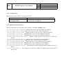
Change record
Issue/Rev.
1
2
Date
2014-05-30
2014-07-01
3
4
5
6
2014-07-08
2014-11-21
2014-11-27
2015-01-23
7
8
2015-03-11
2015-04-07
9
2015-04-28
Section/Parag. affected
All
1.6, 3.3
7.3
4, 8.2
6.6.3, 6.6.4
2, 6.3
All
9.4, 9.12
7
All
All
Reason/Initiation/Documents/Remarks
First version
References to Reflex documentation added
New pixel table handling tool added
Added failed tracing recovery procedure for SV data
Correct typing error in environment variable name
Updated to version 1.0 of the MUSE pipeline
Comments incorporated
Section on legacy calibrations added.
Software release number updated
Updated to version 1.0.3 of the MUSE pipeline
Typing error fixed
Software release number updated
Software release number updated
This page was intentionally left blank
ESO
MUSE Pipeline User Manual
Doc:
Issue:
Date:
Page:
VLT-MAN-ESO-14670-6186
Issue 9
Date 2015-04-28
5 of 132
Contents
1
2
3
Introduction
13
1.1
Scope . . . . . . . . . . . . . . . . . . . . . . . . . . . . . . . . . . . . . . . . . . . . . . . . 13
1.2
Acknowledgements . . . . . . . . . . . . . . . . . . . . . . . . . . . . . . . . . . . . . . . . . 13
1.3
Stylistic Conventions . . . . . . . . . . . . . . . . . . . . . . . . . . . . . . . . . . . . . . . . 13
1.4
Notational Conventions . . . . . . . . . . . . . . . . . . . . . . . . . . . . . . . . . . . . . . . 13
1.5
Reference Documents . . . . . . . . . . . . . . . . . . . . . . . . . . . . . . . . . . . . . . . . 14
1.6
Abbreviations and Acronyms . . . . . . . . . . . . . . . . . . . . . . . . . . . . . . . . . . . . 15
Overview
16
2.1
The MUSE Instrument . . . . . . . . . . . . . . . . . . . . . . . . . . . . . . . . . . . . . . . 16
2.2
The MUSE Data Reduction Pipeline . . . . . . . . . . . . . . . . . . . . . . . . . . . . . . . . 16
Installation
20
3.1
System Requirements – Please Read Carefully! . . . . . . . . . . . . . . . . . . . . . . . . . . 20
3.2
Installing the Software . . . . . . . . . . . . . . . . . . . . . . . . . . . . . . . . . . . . . . . 21
3.3
Toolchain Support . . . . . . . . . . . . . . . . . . . . . . . . . . . . . . . . . . . . . . . . . . 21
3.4
Hints on Running the MUSE Pipeline Recipes . . . . . . . . . . . . . . . . . . . . . . . . . . . 22
3.5
Hints on Using 3rd-Party Tools . . . . . . . . . . . . . . . . . . . . . . . . . . . . . . . . . . . 22
4
Known Issues
24
5
Data Description
25
6
5.1
Raw Data . . . . . . . . . . . . . . . . . . . . . . . . . . . . . . . . . . . . . . . . . . . . . . 25
5.2
Static Calibration Data . . . . . . . . . . . . . . . . . . . . . . . . . . . . . . . . . . . . . . . 25
5.3
Pipeline Products . . . . . . . . . . . . . . . . . . . . . . . . . . . . . . . . . . . . . . . . . . 27
5.3.1
MUSE Images . . . . . . . . . . . . . . . . . . . . . . . . . . . . . . . . . . . . . . . 27
5.3.2
MUSE Pixel Tables . . . . . . . . . . . . . . . . . . . . . . . . . . . . . . . . . . . . . 27
5.3.3
MUSE Data Cubes . . . . . . . . . . . . . . . . . . . . . . . . . . . . . . . . . . . . . 27
5.3.4
Combined Product Data . . . . . . . . . . . . . . . . . . . . . . . . . . . . . . . . . . 28
Data Reduction Cookbook
29
ESO
VLT-MAN-ESO-14670-6186
Issue 9
Date 2015-04-28
6 of 132
6.1
Getting Started with EsoRex . . . . . . . . . . . . . . . . . . . . . . . . . . . . . . . . . . . . 29
6.2
Data Organization . . . . . . . . . . . . . . . . . . . . . . . . . . . . . . . . . . . . . . . . . . 30
6.3
6.2.1
Useful Header Keywords . . . . . . . . . . . . . . . . . . . . . . . . . . . . . . . . . . 30
6.2.2
Data Classification and Association . . . . . . . . . . . . . . . . . . . . . . . . . . . . 31
Basic Reduction . . . . . . . . . . . . . . . . . . . . . . . . . . . . . . . . . . . . . . . . . . . 33
6.3.1
Bias . . . . . . . . . . . . . . . . . . . . . . . . . . . . . . . . . . . . . . . . . . . . . 33
6.3.2
Dark . . . . . . . . . . . . . . . . . . . . . . . . . . . . . . . . . . . . . . . . . . . . . 34
6.3.3
Flat Field . . . . . . . . . . . . . . . . . . . . . . . . . . . . . . . . . . . . . . . . . . 36
6.3.4
Wavelength Calibration . . . . . . . . . . . . . . . . . . . . . . . . . . . . . . . . . . . 36
6.3.5
Line Spread Function . . . . . . . . . . . . . . . . . . . . . . . . . . . . . . . . . . . . 38
6.3.6
Instrument Geometry . . . . . . . . . . . . . . . . . . . . . . . . . . . . . . . . . . . . 40
6.3.7
Illumination Correction . . . . . . . . . . . . . . . . . . . . . . . . . . . . . . . . . . . 40
6.4
Observation Pre-processing . . . . . . . . . . . . . . . . . . . . . . . . . . . . . . . . . . . . . 41
6.5
Observation Post-Processing . . . . . . . . . . . . . . . . . . . . . . . . . . . . . . . . . . . . 42
6.6
7
MUSE Pipeline User Manual
Doc:
Issue:
Date:
Page:
6.5.1
Flux Calibration . . . . . . . . . . . . . . . . . . . . . . . . . . . . . . . . . . . . . . 42
6.5.2
Sky Creation . . . . . . . . . . . . . . . . . . . . . . . . . . . . . . . . . . . . . . . . 44
6.5.3
Astrometry . . . . . . . . . . . . . . . . . . . . . . . . . . . . . . . . . . . . . . . . . 45
6.5.4
Science Observations . . . . . . . . . . . . . . . . . . . . . . . . . . . . . . . . . . . . 46
Combining Exposures . . . . . . . . . . . . . . . . . . . . . . . . . . . . . . . . . . . . . . . . 47
6.6.1
Correcting Coordinate Offsets . . . . . . . . . . . . . . . . . . . . . . . . . . . . . . . 47
6.6.2
Limiting Wavelength Ranges . . . . . . . . . . . . . . . . . . . . . . . . . . . . . . . . 48
6.6.3
Combining Exposures using muse_scipost . . . . . . . . . . . . . . . . . . . . . . . . . 48
6.6.4
Combining Exposures using muse_exp_combine . . . . . . . . . . . . . . . . . . . . . 49
Tips & Tricks
52
7.1
Restricting wavelength ranges . . . . . . . . . . . . . . . . . . . . . . . . . . . . . . . . . . . 52
7.2
Verification Tools . . . . . . . . . . . . . . . . . . . . . . . . . . . . . . . . . . . . . . . . . . 52
7.3
7.2.1
Verification of the tracing solution . . . . . . . . . . . . . . . . . . . . . . . . . . . . . 52
7.2.2
Verification of the wavelength solution . . . . . . . . . . . . . . . . . . . . . . . . . . 54
Miscellaneous Tools . . . . . . . . . . . . . . . . . . . . . . . . . . . . . . . . . . . . . . . . 56
7.3.1
Handling of MUSE pixel tables . . . . . . . . . . . . . . . . . . . . . . . . . . . . . . 56
ESO
8
9
MUSE Pipeline User Manual
Doc:
Issue:
Date:
Page:
VLT-MAN-ESO-14670-6186
Issue 9
Date 2015-04-28
7 of 132
7.3.2
Handling of MUSE bad pixel maps . . . . . . . . . . . . . . . . . . . . . . . . . . . . 57
7.3.3
Working with Data Cubes . . . . . . . . . . . . . . . . . . . . . . . . . . . . . . . . . 58
Troubleshooting
61
8.1
Typical Problems . . . . . . . . . . . . . . . . . . . . . . . . . . . . . . . . . . . . . . . . . . 61
8.2
Failed Tracing . . . . . . . . . . . . . . . . . . . . . . . . . . . . . . . . . . . . . . . . . . . . 61
8.3
The Logfile . . . . . . . . . . . . . . . . . . . . . . . . . . . . . . . . . . . . . . . . . . . . . 62
8.4
Debugging Options . . . . . . . . . . . . . . . . . . . . . . . . . . . . . . . . . . . . . . . . . 63
Recipe Reference
9.1
9.2
9.3
9.4
64
muse_bias . . . . . . . . . . . . . . . . . . . . . . . . . . . . . . . . . . . . . . . . . . . . . . 64
9.1.1
Description . . . . . . . . . . . . . . . . . . . . . . . . . . . . . . . . . . . . . . . . . 64
9.1.2
Input frames . . . . . . . . . . . . . . . . . . . . . . . . . . . . . . . . . . . . . . . . 64
9.1.3
Recipe parameters . . . . . . . . . . . . . . . . . . . . . . . . . . . . . . . . . . . . . 64
9.1.4
Product frames . . . . . . . . . . . . . . . . . . . . . . . . . . . . . . . . . . . . . . . 65
9.1.5
Quality control parameters . . . . . . . . . . . . . . . . . . . . . . . . . . . . . . . . . 66
muse_dark . . . . . . . . . . . . . . . . . . . . . . . . . . . . . . . . . . . . . . . . . . . . . . 67
9.2.1
Description . . . . . . . . . . . . . . . . . . . . . . . . . . . . . . . . . . . . . . . . . 67
9.2.2
Input frames . . . . . . . . . . . . . . . . . . . . . . . . . . . . . . . . . . . . . . . . 67
9.2.3
Recipe parameters . . . . . . . . . . . . . . . . . . . . . . . . . . . . . . . . . . . . . 67
9.2.4
Product frames . . . . . . . . . . . . . . . . . . . . . . . . . . . . . . . . . . . . . . . 68
9.2.5
Quality control parameters . . . . . . . . . . . . . . . . . . . . . . . . . . . . . . . . . 69
muse_flat . . . . . . . . . . . . . . . . . . . . . . . . . . . . . . . . . . . . . . . . . . . . . . 70
9.3.1
Description . . . . . . . . . . . . . . . . . . . . . . . . . . . . . . . . . . . . . . . . . 70
9.3.2
Input frames . . . . . . . . . . . . . . . . . . . . . . . . . . . . . . . . . . . . . . . . 70
9.3.3
Recipe parameters . . . . . . . . . . . . . . . . . . . . . . . . . . . . . . . . . . . . . 70
9.3.4
Product frames . . . . . . . . . . . . . . . . . . . . . . . . . . . . . . . . . . . . . . . 72
9.3.5
Quality control parameters . . . . . . . . . . . . . . . . . . . . . . . . . . . . . . . . . 72
muse_wavecal . . . . . . . . . . . . . . . . . . . . . . . . . . . . . . . . . . . . . . . . . . . . 74
9.4.1
Description . . . . . . . . . . . . . . . . . . . . . . . . . . . . . . . . . . . . . . . . . 74
9.4.2
Input frames . . . . . . . . . . . . . . . . . . . . . . . . . . . . . . . . . . . . . . . . 74
ESO
9.5
9.6
9.7
9.8
9.9
MUSE Pipeline User Manual
Doc:
Issue:
Date:
Page:
VLT-MAN-ESO-14670-6186
Issue 9
Date 2015-04-28
8 of 132
9.4.3
Recipe parameters . . . . . . . . . . . . . . . . . . . . . . . . . . . . . . . . . . . . . 75
9.4.4
Product frames . . . . . . . . . . . . . . . . . . . . . . . . . . . . . . . . . . . . . . . 76
9.4.5
Quality control parameters . . . . . . . . . . . . . . . . . . . . . . . . . . . . . . . . . 77
muse_lsf . . . . . . . . . . . . . . . . . . . . . . . . . . . . . . . . . . . . . . . . . . . . . . . 78
9.5.1
Description . . . . . . . . . . . . . . . . . . . . . . . . . . . . . . . . . . . . . . . . . 78
9.5.2
Input frames . . . . . . . . . . . . . . . . . . . . . . . . . . . . . . . . . . . . . . . . 78
9.5.3
Recipe parameters . . . . . . . . . . . . . . . . . . . . . . . . . . . . . . . . . . . . . 78
9.5.4
Product frames . . . . . . . . . . . . . . . . . . . . . . . . . . . . . . . . . . . . . . . 79
9.5.5
Quality control parameters . . . . . . . . . . . . . . . . . . . . . . . . . . . . . . . . . 79
muse_geometry . . . . . . . . . . . . . . . . . . . . . . . . . . . . . . . . . . . . . . . . . . . 80
9.6.1
Description . . . . . . . . . . . . . . . . . . . . . . . . . . . . . . . . . . . . . . . . . 80
9.6.2
Input frames . . . . . . . . . . . . . . . . . . . . . . . . . . . . . . . . . . . . . . . . 80
9.6.3
Recipe parameters . . . . . . . . . . . . . . . . . . . . . . . . . . . . . . . . . . . . . 80
9.6.4
Product frames . . . . . . . . . . . . . . . . . . . . . . . . . . . . . . . . . . . . . . . 81
9.6.5
Quality control parameters . . . . . . . . . . . . . . . . . . . . . . . . . . . . . . . . . 81
muse_twilight . . . . . . . . . . . . . . . . . . . . . . . . . . . . . . . . . . . . . . . . . . . . 83
9.7.1
Description . . . . . . . . . . . . . . . . . . . . . . . . . . . . . . . . . . . . . . . . . 83
9.7.2
Input frames . . . . . . . . . . . . . . . . . . . . . . . . . . . . . . . . . . . . . . . . 83
9.7.3
Recipe parameters . . . . . . . . . . . . . . . . . . . . . . . . . . . . . . . . . . . . . 84
9.7.4
Product frames . . . . . . . . . . . . . . . . . . . . . . . . . . . . . . . . . . . . . . . 86
9.7.5
Quality control parameters . . . . . . . . . . . . . . . . . . . . . . . . . . . . . . . . . 86
muse_scibasic . . . . . . . . . . . . . . . . . . . . . . . . . . . . . . . . . . . . . . . . . . . . 87
9.8.1
Description . . . . . . . . . . . . . . . . . . . . . . . . . . . . . . . . . . . . . . . . . 87
9.8.2
Input frames . . . . . . . . . . . . . . . . . . . . . . . . . . . . . . . . . . . . . . . . 87
9.8.3
Recipe parameters . . . . . . . . . . . . . . . . . . . . . . . . . . . . . . . . . . . . . 88
9.8.4
Product frames . . . . . . . . . . . . . . . . . . . . . . . . . . . . . . . . . . . . . . . 90
9.8.5
Quality control parameters . . . . . . . . . . . . . . . . . . . . . . . . . . . . . . . . . 90
muse_standard . . . . . . . . . . . . . . . . . . . . . . . . . . . . . . . . . . . . . . . . . . . 91
9.9.1
Description . . . . . . . . . . . . . . . . . . . . . . . . . . . . . . . . . . . . . . . . . 91
9.9.2
Input frames . . . . . . . . . . . . . . . . . . . . . . . . . . . . . . . . . . . . . . . . 91
ESO
MUSE Pipeline User Manual
Doc:
Issue:
Date:
Page:
VLT-MAN-ESO-14670-6186
Issue 9
Date 2015-04-28
9 of 132
9.9.3
Recipe parameters . . . . . . . . . . . . . . . . . . . . . . . . . . . . . . . . . . . . . 91
9.9.4
Product frames . . . . . . . . . . . . . . . . . . . . . . . . . . . . . . . . . . . . . . . 92
9.9.5
Quality control parameters . . . . . . . . . . . . . . . . . . . . . . . . . . . . . . . . . 93
9.10 muse_create_sky . . . . . . . . . . . . . . . . . . . . . . . . . . . . . . . . . . . . . . . . . . 94
9.10.1 Description . . . . . . . . . . . . . . . . . . . . . . . . . . . . . . . . . . . . . . . . . 94
9.10.2 Input frames . . . . . . . . . . . . . . . . . . . . . . . . . . . . . . . . . . . . . . . . 94
9.10.3 Recipe parameters . . . . . . . . . . . . . . . . . . . . . . . . . . . . . . . . . . . . . 94
9.10.4 Product frames . . . . . . . . . . . . . . . . . . . . . . . . . . . . . . . . . . . . . . . 95
9.10.5 Quality control parameters . . . . . . . . . . . . . . . . . . . . . . . . . . . . . . . . . 95
9.11 muse_astrometry . . . . . . . . . . . . . . . . . . . . . . . . . . . . . . . . . . . . . . . . . . 96
9.11.1 Description . . . . . . . . . . . . . . . . . . . . . . . . . . . . . . . . . . . . . . . . . 96
9.11.2 Input frames . . . . . . . . . . . . . . . . . . . . . . . . . . . . . . . . . . . . . . . . 96
9.11.3 Recipe parameters . . . . . . . . . . . . . . . . . . . . . . . . . . . . . . . . . . . . . 96
9.11.4 Product frames . . . . . . . . . . . . . . . . . . . . . . . . . . . . . . . . . . . . . . . 97
9.11.5 Quality control parameters . . . . . . . . . . . . . . . . . . . . . . . . . . . . . . . . . 97
9.12 muse_scipost . . . . . . . . . . . . . . . . . . . . . . . . . . . . . . . . . . . . . . . . . . . . 98
9.12.1 Description . . . . . . . . . . . . . . . . . . . . . . . . . . . . . . . . . . . . . . . . . 98
9.12.2 Input frames . . . . . . . . . . . . . . . . . . . . . . . . . . . . . . . . . . . . . . . . 98
9.12.3 Recipe parameters . . . . . . . . . . . . . . . . . . . . . . . . . . . . . . . . . . . . . 99
9.12.4 Product frames . . . . . . . . . . . . . . . . . . . . . . . . . . . . . . . . . . . . . . . 102
9.12.5 Quality control parameters . . . . . . . . . . . . . . . . . . . . . . . . . . . . . . . . . 102
9.13 muse_exp_combine . . . . . . . . . . . . . . . . . . . . . . . . . . . . . . . . . . . . . . . . . 104
9.13.1 Description . . . . . . . . . . . . . . . . . . . . . . . . . . . . . . . . . . . . . . . . . 104
9.13.2 Input frames . . . . . . . . . . . . . . . . . . . . . . . . . . . . . . . . . . . . . . . . 104
9.13.3 Recipe parameters . . . . . . . . . . . . . . . . . . . . . . . . . . . . . . . . . . . . . 104
9.13.4 Product frames . . . . . . . . . . . . . . . . . . . . . . . . . . . . . . . . . . . . . . . 106
9.13.5 Quality control parameters . . . . . . . . . . . . . . . . . . . . . . . . . . . . . . . . . 106
A Data Formats
107
A.1 Raw Data Files . . . . . . . . . . . . . . . . . . . . . . . . . . . . . . . . . . . . . . . . . . . 107
A.1.1 RAW_IMAGE . . . . . . . . . . . . . . . . . . . . . . . . . . . . . . . . . . . . . . . 107
ESO
MUSE Pipeline User Manual
Doc:
Issue:
Date:
Page:
VLT-MAN-ESO-14670-6186
Issue 9
Date 2015-04-28
10 of 132
A.2 Static Calibration Files . . . . . . . . . . . . . . . . . . . . . . . . . . . . . . . . . . . . . . . 109
A.2.1 LINE_CATALOG . . . . . . . . . . . . . . . . . . . . . . . . . . . . . . . . . . . . . 109
A.2.2 SKY_LINES . . . . . . . . . . . . . . . . . . . . . . . . . . . . . . . . . . . . . . . . 109
A.2.3 ASTROMETRY_REFERENCE . . . . . . . . . . . . . . . . . . . . . . . . . . . . . . 110
A.2.4 EXTINCT_TABLE . . . . . . . . . . . . . . . . . . . . . . . . . . . . . . . . . . . . . 111
A.2.5 BADPIX_TABLE . . . . . . . . . . . . . . . . . . . . . . . . . . . . . . . . . . . . . 111
A.2.6 STD_FLUX_TABLE . . . . . . . . . . . . . . . . . . . . . . . . . . . . . . . . . . . . 112
A.2.7 FILTER_LIST . . . . . . . . . . . . . . . . . . . . . . . . . . . . . . . . . . . . . . . 112
A.2.8 TELLURIC_REGIONS . . . . . . . . . . . . . . . . . . . . . . . . . . . . . . . . . . 113
A.3 Recipe Product Files . . . . . . . . . . . . . . . . . . . . . . . . . . . . . . . . . . . . . . . . 114
A.3.1 MUSE_IMAGE . . . . . . . . . . . . . . . . . . . . . . . . . . . . . . . . . . . . . . 114
A.3.2 PIXEL_TABLE . . . . . . . . . . . . . . . . . . . . . . . . . . . . . . . . . . . . . . . 115
A.3.3 DATACUBE . . . . . . . . . . . . . . . . . . . . . . . . . . . . . . . . . . . . . . . . 117
A.3.4 EURO3DCUBE . . . . . . . . . . . . . . . . . . . . . . . . . . . . . . . . . . . . . . 118
A.3.5 TRACE_TABLE . . . . . . . . . . . . . . . . . . . . . . . . . . . . . . . . . . . . . . 119
A.3.6 TRACE_SAMPLES . . . . . . . . . . . . . . . . . . . . . . . . . . . . . . . . . . . . 120
A.3.7 WAVECAL_TABLE . . . . . . . . . . . . . . . . . . . . . . . . . . . . . . . . . . . . 120
A.3.8 WAVECAL_RESIDUALS . . . . . . . . . . . . . . . . . . . . . . . . . . . . . . . . . 121
A.3.9 LSF_PROFILE . . . . . . . . . . . . . . . . . . . . . . . . . . . . . . . . . . . . . . . 121
A.3.10 GEOMETRY_TABLE . . . . . . . . . . . . . . . . . . . . . . . . . . . . . . . . . . . 122
A.3.11 SPOTS_TABLE . . . . . . . . . . . . . . . . . . . . . . . . . . . . . . . . . . . . . . 123
A.3.12 FLUX_TABLE . . . . . . . . . . . . . . . . . . . . . . . . . . . . . . . . . . . . . . . 124
A.3.13 STD_RESPONSE . . . . . . . . . . . . . . . . . . . . . . . . . . . . . . . . . . . . . 124
A.3.14 STD_TELLURIC . . . . . . . . . . . . . . . . . . . . . . . . . . . . . . . . . . . . . . 125
A.3.15 STD_FLUXES . . . . . . . . . . . . . . . . . . . . . . . . . . . . . . . . . . . . . . . 125
A.3.16 AMPL_CONVOLVED . . . . . . . . . . . . . . . . . . . . . . . . . . . . . . . . . . . 126
A.4 Other data files . . . . . . . . . . . . . . . . . . . . . . . . . . . . . . . . . . . . . . . . . . . 126
A.4.1 OUTPUT_WCS . . . . . . . . . . . . . . . . . . . . . . . . . . . . . . . . . . . . . . 126
B Benchmarks
128
B.1 The Reference System . . . . . . . . . . . . . . . . . . . . . . . . . . . . . . . . . . . . . . . 128
ESO
MUSE Pipeline User Manual
Doc:
Issue:
Date:
Page:
VLT-MAN-ESO-14670-6186
Issue 9
Date 2015-04-28
11 of 132
B.2 Benchmark results . . . . . . . . . . . . . . . . . . . . . . . . . . . . . . . . . . . . . . . . . 128
C Performance Tools
129
C.1 Using taskset . . . . . . . . . . . . . . . . . . . . . . . . . . . . . . . . . . . . . . . . . . 129
C.2 Using the Likwid Lightweight Performance Tools . . . . . . . . . . . . . . . . . . . . . . . . . 129
D Calibrations for Commisioning and Science Verification Data
131
E Useful links
132
ESO
MUSE Pipeline User Manual
Doc:
Issue:
Date:
Page:
VLT-MAN-ESO-14670-6186
Issue 9
Date 2015-04-28
12 of 132
ESO
1
1.1
MUSE Pipeline User Manual
Doc:
Issue:
Date:
Page:
VLT-MAN-ESO-14670-6186
Issue 9
Date 2015-04-28
13 of 132
Introduction
Scope
This document is a quick start guide to the processing of MUSE observations using the MUSE Instrument
Pipeline Recipes (also known as the MUSE Data Reduction Software or MUSE DRS). While it is not as detailed
as the full MUSE Pipeline Manual when it comes to how individual processing recipes work, it should guide
the users through the installation of the software, and bring them quickly to the point where they can use the
software tools to create science ready datacubes from raw MUSE data sets.
The processing of MUSE data is extremly demanding with respect to the computing environment. Therefore,
the document describes the system requirements, the installation and the setup of the environment in some detail
in order to avoid the most common pitfalls, and it is strongly recommended that the users reads these sections
before they start working on MUSE data.
This manual refers to the MUSE Data Reduction Software version 1.0.4. The current release has a few known
issues, which are listed in Section 4.
1.2
Acknowledgements
This cookbook is to a large extent based on the MUSE Data Reduction Software Manual, prepared by T. Urrutia,
O. Streicher and P. Weilbacher, for use within the MUSE consortium. We also would like to thank J. Richard,
P. Weilbacher and B. Husemann for providing valuable comments.
1.3
Stylistic Conventions
Throughout this document the following stylistic conventions are used:
bold
italics
teletype
in text sections for commands and other user input which has to be typed as shown
in the text and example sections for parts of the user input which have to be replaced
with real contents
in the text for FITS keywords, program names, file paths, and terminal output, and
as the general style for examples, commands, code, etc
In example sections expected user input is indicated by a leading shell prompt.
In the text bold and italics may also be used to highlight words.
1.4
Notational Conventions
Hierarchical FITS keyword names, appearing in the document, are given using the dot–notation to improve
readability. This means, that the prefix “HIERARCH ESO” is left out, and the spaces separating the keyword
name constituents in the actual FITS header are replaced by a single dot.
ESO
1.5
MUSE Pipeline User Manual
Doc:
Issue:
Date:
Page:
VLT-MAN-ESO-14670-6186
Issue 9
Date 2015-04-28
14 of 132
Reference Documents
[RD1]
[RD2]
[RD3]
[RD4]
[RD5]
[RD6]
[RD7]
[RD8]
[RD9]
MUSE Pipeline Manual
MUSE User Manual
MUSE Calibration Plan
Gasgano User’s Manual
FITS format description for pipeline products with data, error and
data quality information
The Euro3D Data Format, Kissler-Patig, et al., Issue 1.2, May
2003
3D Visualization Tool Manual
Reflex MUSE Tutorial
Reflex User Manual
TBD
VLT–MAN–ESO–14670–1477
VLT–MAN–ESO–14670–0500
VLT–PRO–ESO-19000–1932
VLT–MAN–ESO–19500–5667
VLT–MAN–ESO–19500–5651
VLT–MAN–ESO–19540–6195
VLT–MAN–ESO–19000–5037
ESO
1.6
MUSE Pipeline User Manual
Abbreviations and Acronyms
AO
CCD
CPL
CPU
DFS
DRS
ESO
EsoRex
FITS
FOV
GCC
GUI
HDU
IFU
LSF
MUSE
NaN
NFM
OpenMP
PAF
pixel
PSF
QC
SGS
SOF
SV
spaxel
TBC
TBD
VLT
voxel
WCS
WFM
Adaptive Optics
Charge Coupled Device
Common Pipeline Library
Central Processing Unit
Data Flow System
Data Reduction System
European Southern Observatory
ESO Recipe Execution Tool
Flexible Image Transport System
Field of View
GNU Compiler Collection
Graphical User Interface
Header Data Unit
Integral Field Unit
Line Spread Function
Multi Unit Spectroscopic Explorer
Not a Number
Narrow Field Mode
Open Multi-Processing
VLT parameter file format
picture element (of a raster image)
Point Spread Function
Quality Control
Slow Guilding System
Set Of Frames
Science Verification
spatial element (of a data cube)
To be confirmed
To be defined
Very Large Telescope
volume element (of a data cube)
World Coordinate System
Wide Field Mode
Doc:
Issue:
Date:
Page:
VLT-MAN-ESO-14670-6186
Issue 9
Date 2015-04-28
15 of 132
ESO
2
2.1
MUSE Pipeline User Manual
Doc:
Issue:
Date:
Page:
VLT-MAN-ESO-14670-6186
Issue 9
Date 2015-04-28
16 of 132
Overview
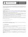
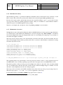
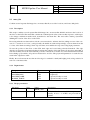
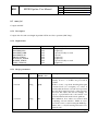
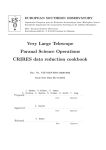
The MUSE Instrument
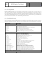
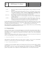
MUSE is an optical wide-field integral field spectrograph that uses the image slicing technique to cover a field
of view (FOV) of 10 × 10 in wide-field mode (WFM) with a sampling of 0.200 × 0.200 spaxels. The full field is
split up into 24 sub-fields (each 2.500 × 6000 in WFM) which are fed into one of the 24 integral field units (IFUs)
of the instrument. Each IFU illuminates a 4k x 4k CCD by separating the incoming light into 48 slices. This is
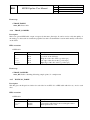
illustrated in Figure 2.1.
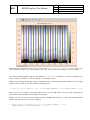
On the CCD, the slices appear as approximately 76.5 pixel wide vertical bands, separated by gaps of about
6 pixel. At the edges of the detector the slices are slightly curved outwards (up to 2 pixel). The slices are offset
vertically, i.e. along the wavelength axis, forming a repetitive, horizontal pattern of three steps. This pattern is
affected by curvature across the CCD, which results in a different wavelength coverage for each slice.
For performance reasons the MUSE detectors are always read in 4-port mode. All four quadrants have equal
size, and are visible in the raw data images separated horizontally and vertically by pre-scan and over-scan
regions. On the detectors, and the raw images the dispersion axis is oriented along the pixel columns (vertical
axis) with the red end of the spectrum at the top, and the blue end at the bottom. The pixel rows (horizontal
axis) correspond to the spatial axis.
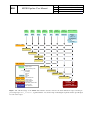
2.2
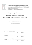
The MUSE Data Reduction Pipeline
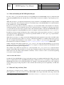
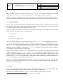
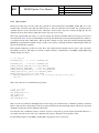
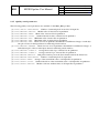
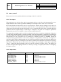
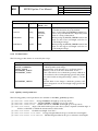
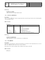
The MUSE pipeline is basically divided into two stages. The first stage consists of the seven basic calibration
recipes and a preprocessing recipe (basic science reduction) which work on the data of individual CCDs to
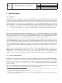
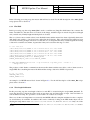
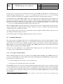
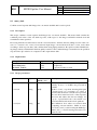
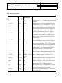
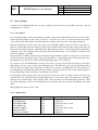
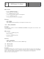
determine and/or remove the signature of each IFU. The recipes of the second stage, another three calibration
recipes and the final science recipe, use the pre-processed data from the first stage and transform it into physical
quantities which can be used for science. These second stage recipes combine the data from all IFUs of one or
more exposures into the final data cube. The two stages of the reduction process are illustrated in Figure 2.2 and
Figure 2.3.
ESO
MUSE Pipeline User Manual
Doc:
Issue:
Date:
Page:
VLT-MAN-ESO-14670-6186
Issue 9
Date 2015-04-28
17 of 132
Figure 2.1: Graphical representations of the splitting and slicing procedures in the MUSE instrument. The example
shown is for wide-field mode; narrow-field mode operates in the same way with a scaled-down field size. Note that the
sizes given are approximate, the real data does not exactly cover a square region on the sky.
ESO
Doc:
Issue:
Date:
Page:
MUSE Pipeline User Manual
VLT-MAN-ESO-14670-6186
Issue 9
Date 2015-04-28
18 of 132
muse_
bias
muse_
dark
muse_
flat
muse_
wavecal
muse_
lsf
muse_
geometry
BIAS
DARK
FLAT
ARC
ARC
MASK
muse_
muse_scibasic
twilight
SKYFLAT
OBJECT,
STD,
SKY, or
ASTROMETRY
optional +
ILLUM
BADPIX_TABLE
MASTER_BIAS
MASTER_DARK
MASTER_FLAT
TRACE_TABLE
LINE_CATALOG
muse_lsf
pipeline recipe
recipe processing order
association
WAVECAL_TABLE
LSF_PROFILE
mandatory
SKYFLAT
BADPIX_TABLE
TRACE_TABLE
optional
input:
raw data
input:
external/static data
output product:
master calibration
output product:
PIXTABLE_SKY intermediate reduced data
DATA_CUBE
output product:
final output data
GEOMETRY_TABLE
TWILIGHT_CUBE
PIXTABLE_OBJECT
PIXTABLE_STD
PIXTABLE_SKY
PIXTABLE_ASTROMETRY
Figure 2.2: The first stage of the MUSE data reduction cascade. It shows the basic calibration recipes and the preprocessing recipe muse_scibasic, together with the “Association map” indicating the required and the optional input
for each of the recipes.
ESO
Doc:
Issue:
Date:
Page:
MUSE Pipeline User Manual
muse_
standard
muse_
create_sky
24x
24x
PIXTABLE_
SKY
PIXTABLE_
STD
muse_
astrometry
24x
PIXTABLE_
ASTROMETRY
VLT-MAN-ESO-14670-6186
Issue 9
Date 2015-04-28
19 of 132
muse_
scipost
n x 24x
PIXTABLE_
OBJECT
STD_FLUX_TABLE
EXTINCT_TABLE
STD_RESPONSE
STD_TELLURIC
LSF_PROFILE
SKY_LINES
SKY_CONTINUUM
ASTROMETRY_REFERENCE
muse_
exp_combine
ASTROMETRY_WCS
PIXTABLE_REDUCED
several
DATACUBE_FINAL
DATACUBE_FINAL
(multiple)
(multiple)
FILTER_LIST
muse_lsf
pipeline recipe
IMAGE_FOV
IMAGE_FOV
recipe processing order
association
mandatory
SKYFLAT
BADPIX_TABLE
TRACE_TABLE
optional
input:
raw data
input:
external/static data
output product:
master calibration
output product:
PIXTABLE_SKY intermediate reduced data
DATA_CUBE
output product:
final output data
Figure 2.3: The second stage of the MUSE data reduction cascade. These recipes start from the output of the preprocessing recipe muse_scibasic and combine the data from all 24 IFUs into a single, fully reduced and calibrated
data cube. Again the “Association map” indicates the required and the optional input for each of the recipes.
ESO
3
3.1
MUSE Pipeline User Manual
Doc:
Issue:
Date:
Page:
VLT-MAN-ESO-14670-6186
Issue 9
Date 2015-04-28
20 of 132
Installation
System Requirements – Please Read Carefully!
The processing of MUSE data is very demanding in terms of computing resources. In particular it requires a
machine with sufficient memory installed. Less critical but still important is the number of available CPU cores
and the amount of available disk space.
Because of the memory constraints, the MUSE DRS is only supported on 64-bit platforms. The recommended
platform is a powerful workstation with a recent 64-bit Linux system.
The minimum system configuration is:
• 32 GB of memory
• 4 CPU cores (physical cores)
• 1 TB of free disk space
• GCC 4.4.6 (or newer)
The recommended configuration of the target machine for creating the final data cube from a single MUSE
observation and the required set of calibrations is:
• 64 GB of memory
• 24 CPU cores (physical cores)
• 4 TB of free disk space
• GCC 4.8.2 (or newer)
The peak memory consumption depends on the number of input exposures used and the size of the final data
cube. When a data cube is created from a single MUSE exposure the peak memory usage may vary between
approximately 18 GB and 25 GB depending on the orientation of the field of view. Peak memory consumption
is reached at a rotation angle of ±45◦ and ±135◦ with respect to North. On disk the size of the final data cube
file may vary between 4 GB and 5.3 GB for a single observation.
If it is forseen to combine several MUSE observations, the memory needed depends on the maximum number of
observations to combine. In general the memory consumption grows linearly with the number of observations.
Finally, when it comes to creating MUSE mosaics, one should be aware that the size of the data cube may
become really huge, and the required memory grows accordingly! For details on combining MUSE exposures
refer to Section 6.6.
The same memory requirements apply to the MUSE calibration recipes. The minimum memory estimate of
32 GB given before is suitable for processing standard calibration sets of 5 exposures. Adding exposures to the
input of the recipes requires additional memory.
ESO
MUSE Pipeline User Manual
Doc:
Issue:
Date:
Page:
VLT-MAN-ESO-14670-6186
Issue 9
Date 2015-04-28
21 of 132
However, since the calibration recipes can work on a single IFU at a time, the memory requirements can be
relaxed for these recipes at the price of reduced performance. For the creation of the final data cube the only
possibility to reduce the required memory is to limit the wavelength range of the output data cube to an appropriate size (cf. Section 7.1).
3.2
Installing the Software
The MUSE Data Reduction Software is distributed as a standard pipeline kit package and can be obtained from
the ESO web pages at http://www.eso.org/sci/software/pipelines. Apart from the MUSE
DRS itself, the distributed package contains all dependencies needed for the installation, the tools to run the
MUSE DRS recipes, this cookbook, and the installer utility for the kit.
Using the installer the MUSE DRS can be installed on recent versions of any major Linux distribution, as well
as Mac OS X. However, the recommended target platform for using the MUSE DRS is a 64-bit Linux system,
since Mac OS X imposes certain restrictions when it comes to running the MUSE DRS.
To install the MUSE DRS unpack the kit in a temporary location, go to the top level directory of the unpacked
distribution package and execute the installer script as shown in the following example.
Note: The installation script uses the compiler which is found first in the path! If more than one compiler are
installed on the system one should make sure that an appropriate 64-bit compiler will be found first when the
installation script is executed!
1> tar -zxf muse-kit-X.Y.Z.tar.gz
2> cd muse-kit-X.Y.Z.tar.gz
3> ./install_pipeline
Then follow the instructions on the screen. Once the script finishes successfully and the path variables have
been set, the installation of the MUSE DRS is complete.
3.3
Toolchain Support
ESO offers three different tools to process data obtained with one of the VLT instruments. One command line
tool EsoRex, and two GUI based tools, Gasgano and Reflex respectively.
This manual will focus on the EsoRex command line tool, which offers a manual control on the reduction
process.
We recommend the user to use Reflex and the MUSE workflow to process MUSE observations, as this offers
a convenient way to execute a fixed setup of the reduction chain and it includes automatic data organisation as
well as the alignment and co-adding of exposures. See [RD8] and [RD9] for details on how to use the MUSE
Reflex workflow and Reflex itself.
While Gasgano is useful as file browser for exploring MUSE data sets, it is not recommended to use it to run
the MUSE DRS recipes. Using Gasgano to run MUSE recipes will therefore not be discussed further in this
manual.
ESO
3.4
MUSE Pipeline User Manual
Doc:
Issue:
Date:
Page:
VLT-MAN-ESO-14670-6186
Issue 9
Date 2015-04-28
22 of 132
Hints on Running the MUSE Pipeline Recipes
In order to have a good performance when processing MUSE data, the MUSE DRS recipes are multi-threaded
using the OpenMP thread model, and thus may use all the CPU cores that are available to speed up the processing.
While this mode has to be explicitly enabled using a recipe parameter for the MUSE calibration recipes and the
preprocessing recipe, this is always used in the second stage recipes of the MUSE DRS. It is assumed that this
is the standard way to run the MUSE DRS.
However, it is not always the best solution to simply try to use all available CPUs on the machine. For instance,
reducing the number of allowed threads can be used to reduce the memory consumption of the first stage recipes
(of course this increases the recipes execution time). The maximum number of threads the MUSE DRS recipes
(actually any application using OpenMP) may can be set using the environment variable OMP_NUM_THREADS1 .
In addition, modern computer architectures have certain features which may make it necessary to control the
way high performance applications are executed on a particular machine, in order to get to a good performance.
This applies also to the MUSE DRS.
What may be necessary is to make sure that the individual threads the application runs stick to the CPU where
they were started in first place. There are several so called thread pinning tools available which can be used for
this. For example Linux distributions come with the taskset utility, or, one can use the Likwid Lightweight
Performance Tools which are available at https://code.google.com/p/likwid (Linux only!).
Neither setting the environment variable OMP_NUM_THREADS nor using any thread-pinning tool is necessary
as long as one gets a good performance. To allow for a comparison of the performance, the benchmarks for the
ESO baseline system are given in Appendix B.
The standard setup at ESO are 24 threads (i.e. 1 thread per IFU, OMP_NUM_THREADS=24) with the threads
pinned to the machines physical CPU cores for all recipes (with the exception of the geometric calibration recipe
which can be run only with a reduced number of threads). A short overview on how to use the thread pinning
tools can be found in Appendix C.
A Note for Mac OS X Users
On Mac OS X the MUSE DRS is always built without support for running multi-threaded. This is due to the
lack of essential features in the OpenMP implementation of Mac OS X. As a consequence on Mac OS X the
MUSE DRS will always run in single-threaded mode. Turning on the multi-threaded mode for the calibration
recipes and the preprocessing recipe has no effect, and the data would be processed sequentially, one IFU after
the other.
3.5
Hints on Using 3rd-Party Tools
Any 3rd-party tool which is used to visualize, or inspect the product files created by the MUSE DRS should be
64-bit applications, since the products from the MUSE DRS can be larger than 2 GB. Files larger than 2 GB
1 Actually for some implementations the default maximum number of threads is 1 or 2. In this case OMP_NUM_THREADS must be
used to enlarge the number of allowed threads.
ESO
MUSE Pipeline User Manual
Doc:
Issue:
Date:
Page:
VLT-MAN-ESO-14670-6186
Issue 9
Date 2015-04-28
23 of 132
cannot be handled by 32-bit applications, unless they have been specifically build for that.
This applies in particular to the visualization tool used to inspect the final data cube product with file sizes of
4 GB or more.
ESO
4
MUSE Pipeline User Manual
Doc:
Issue:
Date:
Page:
VLT-MAN-ESO-14670-6186
Issue 9
Date 2015-04-28
24 of 132
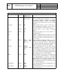
Known Issues
The MUSE Pipeline is continuously improved. The release notes including the latest improvments and changes
is always available at http://www.eso.org/sci/software/pipelines/muse. In addition this sections summarizes the most critical issues which are known at the time the release has been made.
Users processing MUSE data with the MUSE DRS version 1.0.4 should be aware of the following known issues:
• The sky subtraction is currently not optimal and may leave artifacts due to the current parametrization of
the line spread function. An alternative method is being worked on, but it still needs to be fully validated.
This issue has the highest priority, and an update will be made available as soon as possible!
• The tools described in section 7.2 and section 7.3 do not yet work with pipeline products saved using the
combined data format, i.e. to use them the recipes have to be run without the option --merge.
• In general the recipe muse_astrometry works without problems, but it may occasionally fail to identify
(enough) stars depending on the observing conditions. Using a smaller value for the recipe parameter
--detsigma may solve this. Once muse_astrometry finishes sucessfully, it is recommended to verify
that the derived pixel scale is close to the nominal value of 0.2 00 /spaxel. The measured pixel scale is stored
as the FITS keywords QC.ASTRO.SCALE.X and QC.ASTRO.SCALE.Y of the astrometric solution.
In any case, it is always a safe alternative to use the astrometric solution shipped with the pipeline distribution kit.
• The cosmic ray rejection has been improved substantially. However the default settings are chosen to be
conservative so that no real data gets rejected. However, more aggressive settings may be used to optimize
the results of the cosmic ray rejection for individual exposures.
Another issue, specifically affects data taken during the first MUSE Science Verification run. For flat fields,
which are taken at low ambient temperature (temperatures lower than ≈ 7 ◦ C), the tracing of the edges of the
slices may fail. Data taken after this first SV run should not be affected since the issue will be fixed at the
instrument level.
In order to be able to complete the processing of the SV data if such a failure happens if muse_flat, a recovery
procedure is described in Section 8.2.
ESO
5
MUSE Pipeline User Manual
Doc:
Issue:
Date:
Page:
VLT-MAN-ESO-14670-6186
Issue 9
Date 2015-04-28
25 of 132
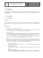
Data Description
5.1
Raw Data
The MUSE raw data of all 24 IFUs is stored in a single FITS file as individual FITS extensions. When MUSE
raw data is retrieved from the ESO archive they will have the standard ESO archive file names which are made
up of instrument identifier followed by a time stamp. The time stamp corresponds to the contents of the FITS
header keywords MJD-OBS and DATE-OBS respectively, i.e. to the date and time when the exposure has been
taken (a difference of 1 ms between the file name and the contents of the keywords may be present). In the
case of MUSE, the files returned by the archive are tile compressed, which is indicated by the file name suffix
.fits.fz instead of the regular .fits suffix, so that the file name of a MUSE raw data file will look like
MUSE.2014-02-20T23:31:38.542.fits.fz
These tile compressed files may be unpacked using the funpack tool which is distributed as part of the CFITSIO package (see Section E for the web site). If the MUSE DRS recipes are executed directly from the command
line using EsoRex there is no need to uncompress the MUSE raw data files, since the MUSE DRS will do this
on the fly. This is however not true for Reflex which works only on the uncompressed files2 .
The MUSE raw data files are composed of 24 FITS extensions, one for each IFU, which contain the detector
data and the IFU/detector specific keywords, and a primary FITS HDU which contains only keywords. The
keywords in this primary HDU contain almost all the information which is needed to correctly identify and
process the individual files. In addition, science exposures will contain an extra three FITS extensions which
contain information from the MUSE Slow Guiding System (SGS), if the SGS is activated (see Section A for
details).
The 24 extensions containing the detector data of the IFUs can be identified using the contents of the EXTNAME
FITS keyword. The extensions are called CHAN013 , CHAN02, etc. For technical reasons, the numbering of
the FITS extensions does not correspond to the numbering of the MUSE channels, so that individual channels
should be looked up by name. However, the sequence of the channels as they are stored in the FITS file is fixed.
5.2
Static Calibration Data
In addition to the calibration data which are created by the MUSE calibration recipes the MUSE DRS requires
a number of so called “static” calibrations4 , which are prepared manually, and which are part of the MUSE
DRS distribution package. After the installation procedure is complete, the static calibrations are located in
<installation prefix>/calib/muse-X.Y.Z/cal unless a different place has been specified during the installation.
The set of static calibrations is summarized in the following with short description of the contents of each of the
files. For a detailed description of the data layout please refer to Appendix A.
2 Due
to the format of the MUSE raw data files, it is actually possible to use the compressed files, if the suffix .fz is removed.
However, in general (other instruments), this may not work!
3 The term “channel” is equivalent to IFU and the two terms may be used interchangably.
4 Here “static” means that these files are not created by a recipe, but prepared manually by other means. They may however change
from one pipeline release to the next.
ESO
MUSE Pipeline User Manual
Doc:
Issue:
Date:
Page:
VLT-MAN-ESO-14670-6186
Issue 9
Date 2015-04-28
26 of 132
astrometry_reference.fits
The catalog positions of the astrometric reference object for all the
fields used according to the MUSE calibration plan. Each field is
stored in a separate extension.
badpix_table.fits
The detector positions of well known bad pixels. The data for each
channel is stored in a separate extension. The positions listed here
will be propagated as part of the data quality extension of the product
files.
extinct_table.fits
Atmospheric extinction at the Paranal observatory as a function of
wavelength [Å] in units of mag airmass−1 .
filter_list.fits
The filter transmission as a function of wavelength [Å] for various
filters which are used to define the wavelength band for the reconstruction of field-of-view images from the observed spectra. Each
transmission curve is stored in a separate extension.
line_catalog.fits
A list of air wavelengths [Å] of arc lamp lines. Additional information on relative flux, originating ion and line “quality” flags are also
present and may be used by the DRS.
geometry_table_wfm.fits
The wide-field mode geometrical calibration, i.e. the mapping of the
individual slices from the CCD of each IFU into the MUSE field-ofview
sky_lines.fits
A list of OH line transitions and other sky lines used for modelling
and correction of the sky background.
std_flux_table.fits
The spectra of the spectrophotometric standard stars used according
to the MUSE calibration plan. The spectra of the each standard star
are stored in a separate extension. For each standard star the air
wavelength [Å], the flux [erg s−1 cm−2 Å−1 ] and its error are given.
vignetting_mask.fits
It is a mask to correct for the vignetting which, usually, is present in
the lower right corner of the MUSE field-of-view.
For calibration files like the astrometric catalog, the filter list or the standard flux table, the name of the field,
the filter or the object is the name of the extension and can be obtained by looking up the EXTNAME header
keyword.
In addition to this set of static calibrations, the distribution kit will also contain a few master calibration files,
which in principle can be created using the provided MUSE DRS recipes. These calibration files, the lsf-profiles
(lsf_profile_slow_wfm-n.fits and lsf_profile_slow_wfm-e.fits), the astrometric calibration (astrometry_wcs_wfm.fits), and the two response curves (std_response_wfm-e.fits,
std_response_wfm-n.fits) contain the model of the MUSE line spread function, the WFM astrometric
calibration, and the WFM response curves for the extended and nominal wavelength range respectively. These
files are provided as a convenience since their creation is either very time consuming (lsf-profiles), where found
to be stable in the analysis of the available commissioning data and/or may be used as a fallback solution in
view of the mentioned limitations of the current pipeline version (cf. Section 1.1).
ESO
MUSE Pipeline User Manual
Doc:
Issue:
Date:
Page:
VLT-MAN-ESO-14670-6186
Issue 9
Date 2015-04-28
27 of 132
Strictly speaking also the geometry table could be created using the MUSE DRS. However this requires a large,
specific data set and expert knowledge to get to a good result. Thus the geometry table is, and will be distributed
by ESO as a static calibration.
For static calibrations (geometric calibration and astrometric solution) needed to process observations taken
before December 1st, 2014 please refer to Appendix D.
5.3
Pipeline Products
The MUSE DRS is designed to propagate errors and data quality information together with the processed data
from the beginning to the very end of the data reduction sequence. The errors and data quality information
is stored in the MUSE DRS product files following the convention described in [RD5]. In the following the
general layout of the products carrying this information is summarized. A detailed description of the format of
all products can be found in Appendix A.
5.3.1
MUSE Images
A MUSE image, i.e. the reduced image of a single CCD, as it is, or can be created by almost every MUSE
recipe, has three 2D FITS image extensions:
DATA
DQ
STAT
The reduced image.
The data quality flags encoded in an integer value according to the Euro3D standard (cf. [RD6]).
The variance of the reduced data.
The labels DATA, DQ, and STAT refer to the name of the respective FITS extension (i.e. the EXTNAME keyword).
5.3.2
MUSE Pixel Tables
The pixel table format is used to store the intermediate products of the pre-processing recipe muse_scibasic
and a few post-processing recipes. For each CCD pixel of a single IFU the pixel table records the value of
each pixel together with its “coordinates” (position and wavelength). This format has been introduced to avoid
intermediate re-sampling of the data. The pixel table keeps the un-resampled pixel value until the very end of
the data reduction. What is changed instead in the different processing steps are only the “coordinates” which
are assigned to each pixel. In addition to the value of each CCD pixel and its position, the data quality and the
statistical error are also recorded. Since version 1.0 of the MUSE DRS the default file format of the pixel tables
is based on images in contrast to the table format used in previous releases. This change has been introduced
for performance reasons5 .
5.3.3
MUSE Data Cubes
The final output of the MUSE pipeline are the MUSE data cubes. Similar to the MUSE image format the data
cubes consist of up to three 3D FITS cube (NAXIS=3 volume data) extensions. The FITS cube extensions are
5 In case it should be necessary, the old table format is still available and can be restored by setting the environment variable
MUSE_PIXTABLE_SAVE_AS_TABLE=1
ESO
MUSE Pipeline User Manual
Doc:
Issue:
Date:
Page:
VLT-MAN-ESO-14670-6186
Issue 9
Date 2015-04-28
28 of 132
also named DATA, DQ, and STAT. However, by default, the data quality extension is not present, instead pixels
which do not have a clean data quality status are directly encoded as Not-a-Number (NaN) values in the DATA
extension itself.
In an extended form, the data cube may also contain one or more — one for each selected filter — 2D FITS
image extensions with the reconstructed FOV images and the corresponding variance images. However, by
default the FOV images are saved as individual files in the standard MUSE image format.
5.3.4
Combined Product Data
By default the MUSE calibration recipes write product files which contain the data belonging to a single IFU,
and therefore write 24 files for each kind of product. For example the recipe muse_bias creates 24 master bias
products on disk. This keeps the file size small and the product files can be easily handled by standard tools
(visualization tools, FITS header viewers, etc).
In addition to that there is a combined format for the product files, where the results for the individual IFUs are
stored in a single FITS file, similar to the MUSE raw data files. In this format the extensions are named as in
the individual products with a prefix identifying the IFU from which it originates. For example, a combined
master bias file contains 72 FITS extensions (data, error and data quality extensions for 24 IFUs) which are
called CHAN<nifu>.DATA, CHAN<nifu>.DQ, and CHAN<nifu>.STAT, with nifu = 01 . . . 24.
With the exception of the pixel tables the combined format is available for all pipeline products which would otherwise be saved to disk as 24 individual files. The MUSE recipes can read combined products as well as products
stored as individual files. For different calibrations, the two product formats may even be mixed. For instance the
master calibration files lsf_profile_slow_wfm-n.fits and lsf_profile_slow_wfm-e.fits
which are distributed as part of the MUSE pipeline kit are stored as combined products. As of version 1.0 of the
MUSE DRS the recipe option “--merge” can be used to enable writing recipe products using the combined
format.
ESO
6
6.1
MUSE Pipeline User Manual
Doc:
Issue:
Date:
Page:
VLT-MAN-ESO-14670-6186
Issue 9
Date 2015-04-28
29 of 132
Data Reduction Cookbook
Getting Started with EsoRex
EsoRex is a command-line tool which can be used to execute not only the MUSE DRS recipes, but the recipes
of all standard VLT/VLTI instrument pipelines. With EsoRex in your path, the general structure of an EsoRex
command line is
1> esorex [esorex options] [recipe [recipe options] [sof [sof]...]]
where options appearing before the recipe name are options for EsoRex itself, and options given after the recipe
name are options which affect the recipe.
All available EsoRex options can be listed with the command
1> esorex --help
and the full list of available parameters of a specific recipe can be obtained with the command
1> esorex --help <recipe name>
The output of this command shows as parameter values the current setting, i.e. all modifications from a configuration file or the command line are already applied.
The listing of all recipes known to EsoRex can be obtained with the command
1> esorex --recipes
The last arguments of an EsoRex command are the so-called set-of-frames. A set-of-frames is a simple text
file which contains a list of input data files for the recipe. Each input file is followed by an unique identifier
(frame classification or frame tag), indicating the contents of this file. The input files have to be given as an
absolute path, however EsoRex allows the use of environment variables so that a common directory prefix can
be abreviated. Individual lines may be commented out by putting the hash character (#) in the first column. An
example of a set-of-frames is shown in the following:
1> cat bias.sof
/data/muse/raw/MUSE.2014-02-21T09:48:53.153.fits BIAS
$RAW_DATA/MUSE.2014-02-21T09:50:36.645.fits BIAS
$RAW_DATA/MUSE.2014-02-21T09:52:16.513.fits BIAS
$RAW_DATA/MUSE.2014-02-21T09:53:47.996.fits BIAS
#$RAW_DATA/MUSE.2014-02-21T09:55:04.515.fits BIAS
These set-of-frames files will have to be created by the user using a text editor, for instance. Which classification
has to be used with which recipe will be shown in section 6.2.2.
Finally, if more than one set-of-frames is given on the command-line EsoRex concatenates them into a single
set-of-frames.
ESO
6.2
MUSE Pipeline User Manual
Doc:
Issue:
Date:
Page:
VLT-MAN-ESO-14670-6186
Issue 9
Date 2015-04-28
30 of 132
Data Organization
Running the MUSE pipeline recipes using EsoRex requires that the user prepares the set-of-frames file. To be
able to do this one has to find the correct input files for each recipe and assigns the correct frame tag and one
has to find calibration file which were taken with a matching instrument configuration. The following sections
will summarize which FITS header keywords are useful for that, what are the valid frame tags and which header
keywords should be checked in order to find matching calibration frames.
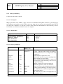
6.2.1
Useful Header Keywords
The following table summarizes FITS header keywords which provide useful information about the observation,
instrument configuration and status. The keywords are grouped by their context and intended use, respectively.
Keyword Name
Description
Keywords for frame classification:
INSTRUME
Name of the instrument
DPR.CATG
DPR.TYPE
DPR.TECH
Raw data frame product category
Raw data frame product type (i.e. the type of observation)
Raw data frame observation technique
TPL.ID
Name of the template used to create the exposure
PRO.CATG
Pipeline product category (i.e. the type of the product)
Keywords describing the observation:
OBJECT
RA
DEC
MJD-OBS
DATE-OBS
Target name
Telescope pointing RA (J2000) [deg]
Telescope pointing DEC (J2000) [deg]
Modified Julien Date at the start of the exposure
Human readable version of MJD-OBS
OBS.NAME
OBS.START
OBS.TARG.NAME
Name of the observation block
Start time of the observation block
Target name
TPL.START
TPL.EXPNO
TPL.NEXP
Start time of the template (within the observation block)
Exposure sequence number within the template
Number of exposures within the template
TEL.AIRM.START
TEL.AIRM.END
TEL.PARANG.START
TEL.PARANG.END
TEL.AMBI.FWHM.START
TEL.AMBI.FWHM.END
TEL.AMBI.RHUM
TEL.AMBI.TEMP
Airmass at exposure start
Airmass at the end of the exposure
Parallactic angle at exposure start (from site monitor)
Parallactic angle at exposure end (from site monitor)
Observatory seeing at exposure start (from site monitor)
Observatory seeing at exposure end (from site monitor)
Observatory ambient relative humidity (from site monitor)
Observatory ambient temperature (from site monitor)
Keywords describing the instrument/detector setup:
EXPTIME
Total integration time [s]
ESO
MUSE Pipeline User Manual
Keyword Name
INS.MODE
Doc:
Issue:
Date:
Page:
VLT-MAN-ESO-14670-6186
Issue 9
Date 2015-04-28
31 of 132
INS.OPTI2.NAME
INS.LAMP1.ST
INS.SHUT1.ST
INS.LAMP2.ST
INS.SHUT2.ST
INS.LAMP3.ST
INS.SHUT3.ST
INS.LAMP4.ST
INS.SHUT4.ST
INS.LAMP5.ST
INS.SHUT5.ST
INS.TEMP4.VAL
Description
Instrument mode (field mode WFM/NFM, AO status, nominal/extended wavelength range)
Wavelength range cutoff filter setting “Blue” or “Clear” for nominal and extended wavelength range, respectively
Field mode setting, “WFM” or “NFM”
Blue continuum lamp on/off
Blue continuum lamp shutter open/closed
Red continuum lamp on/off
Red continuum lamp shutter open/closed
Neon arc lamp on/off
Neon arc lamp shutter open/closed
Xenon arc lamp on/off
Xenon arc lamp shutter open/closed
HgCd arc lamp on/off
HgCd arc lamp shutter open/closed
Ambient temperature [◦ C]
DET.BINX
DET.BINY
DET.READ.CURNAME
DET.CHIP.NAME
DET.CHIP.LIVE
Detector binning along X axis (rows)
Detector binning along Y axis (columns)
Detector readout mode name
Detector chip (instrument channel) name
Detector alive
Other keywords:
EXTNAME
Name of the FITS extension
INS.OPTI1.NAME
Almost all product file which are created by the MUSE pipeline recipes also contain a number of Quality Control
Parameters (QC parameters). These QC parameters are values which are computed by the MUSE recipes as
indicators of the quality of the raw data and the reduction process. They are available from the FITS header of
the pipeline products as hierarchical keywords starting with the leading group component “QC.”.
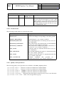
6.2.2
Data Classification and Association
In order to create the set-of-frames for a particular MUSE recipe, both, the raw input data files and the calibration data files have to classified, i.e. the frame tag which indicates the type of data the file contains has to be
determined. The result of this, i.e. the frame tag has to be given in the second column of the set-of-frames (cf.
section 6.1).
The type of a MUSE raw data files is fully determined by a unique combination of the header keywords
DPR.CATG, DPR.TYPE, and DPR.TECH. The type of a MUSE pipeline product is completely determined
by the header keyword PRO.CATG, and the keyword value is also the frame tag to be used in the set-of-frames.
The latter also applies to the static calibration files.
Table 6.1 summarizes the the valid raw data frame tags which are defined for the MUSE, together with the
corresponding combination of DPR keywords and the name of the MUSE recipe used to process them. To
classify MUSE raw data files it is almost always sufficient to just look at the keyword DPR.TYPE. In particular,
the keyword DPR.TECH is always equal to “IFU” for all MUSE raw data files.
Although the input files to the second stage recipes are strictly speaking pipeline product files, and therefore
ESO
MUSE Pipeline User Manual
Doc:
Issue:
Date:
Page:
VLT-MAN-ESO-14670-6186
Issue 9
Date 2015-04-28
32 of 132
Frame tag
Recipe
DPR.CATG
DPR.TYPE
DPR.TECH
BIAS
DARK
FLAT
SKYFLAT
ARC
MASK
STD
ASTROMETRY
SKY
OBJECT
ILLUM
muse_bias
muse_dark
muse_flat
muse_twilight
muse_wavecal
muse_geometry
muse_scibasic
muse_scibasic
muse_scibasic
muse_scibasic
muse_scibasic
CALIB
CALIB
CALIB
CALIB
CALIB
CALIB
CALIB
CALIB
SCIENCE
SCIENCE
CALIB
BIAS
DARK
FLAT,LAMP
FLAT,SKY
WAVE
WAVE,MASK
STD
ASTROMETRY
SKY
OBJECT
FLAT,LAMP,ILLUM
IFU
IFU
IFU
IFU
IFU
IFU
IFU
IFU
IFU
IFU
IFU
Table 6.1: Raw data frame tags of the first stage recipes
their frame tag is given by the value of the keyword PRO.CATG, they are listed in Table 6.2 for the sake of
completeness. Also listed here is a utility recipe which can be used to combine the fully reduced pixel tables
which can be created by muse_scipost as intermediate products (for details see Section 6.5).
Frame tag
PIXTABLE_STD
PIXTABLE_SKY
PIXTABLE_ASTROMETRY
PIXTABLE_OBJECT
PIXTABLE_REDUCED
Recipe
muse_standard
muse_create_sky
muse_astrometry
muse_scipost
muse_exp_combine
PRO.CATG
PIXTABLE_STD
PIXTABLE_SKY
PIXTABLE_ASTROMETRY
PIXTABLE_OBJECT
PIXTABLE_REDUCED
Table 6.2: “Raw” data frame tags of the second stage recipes
Once one has accumulated a substatial number of MUSE files, possibly even spread over several directories, the
Gasgano file browser may be a handy tool to not loose track of the data. Gasgano is able to scan the files in
some specified directories and applies the classification rules for MUSE to them. The resulting frame tag will
then be shown in the Gasgano GUI in the column Classification.
The last step in creating set-of-frames files as input for the MUSE recipes is to find the appropriate calibrations,
both, static calibrations and master calibrations. This means that one has to select calibrations which originate
from the same (or compatible) instrument and/or detector configuration.
The basic set of header keywords which is useful for finding matching calibrations is just made of a few keywords. Since there is only a single detector configuration available for MUSE, there is no real need to verify
that the detector parameters of the raw data frames and the calibrations match (in principle the header keywords
DET.BINX, DET.BINY, and DET.READ.CURID or DET.READ.CURNAME could be used).
To find a calibrations with a matching instrument setup one can use one of the header keywords INS.MODE
and INS.OPTI2.NAME, depending whether the whole instrument configuration should match, or only the
field mode. The keyword INS.MODE provides information on the field mode (wide or narrow field mode),
whether the AO was used, and, whether the nominal or the extended wavelength range (i.e. with or without the
ESO
MUSE Pipeline User Manual
Doc:
Issue:
Date:
Page:
VLT-MAN-ESO-14670-6186
Issue 9
Date 2015-04-28
33 of 132
blue cutoff filter in place) was selected6 . The keyword INS.OPTI2.NAME contains only the setup of the field
mode. It may be used in cases where the other parameters of the instrument setup do not matter.
Finally, if one obtains calibrations as part of an archive request from the ESO archive, then the ESO archive took
already care that they match the raw data of the request. Thus, there may be no need to redo the data association.
6.3
Basic Reduction
Now it is time to start processing the data. During the basic reduction the master calibrations are created from
raw calibration data, and they are applied in the pre-processing step. The different steps of the basic reduction
are shown in Figure 2.2 and will be executed from left to right.
As already mentioned in Section 2.2, the recipes of this first processing stage are working on the data of a single
CCD, and there are basically 3 ways to run the recipes:
• manual mode
• serial mode
• parallel mode (using threads)
where the different modes are selected with the recipe option “--nifu”. For the manual mode one has to
provide the number of the IFU to process, i.e. a number in the range from 1 to 24. With this mode one can
also process several IFUs in parallel by launching more than one EsoRex command. The serial mode is selected
with “--nifu=0”. In this case all IFUs are processed one after the other with a single EsoRex command.
Parallel processing of all IFUs is selected with “--nifu=-1”. All three option can use the same set-of-frames,
provided that it contains the entries for all 24 IFUs.
In the following examples the data is processed in parallel and the recipe products are written using the combined
format, i.e. the recipe options “--nifu=-1” and “--merge” are used in the examples whenever possible. The
prefix command for pinning the threads is omitted in order to keep the command line examples easy to read.
How to call EsoRex with pinning the threads is shown in Section C. For reasons of clarity the environment
variable OMP_NUM_THREADS is explicitly set for each EsoRex command, although it would be sufficient to do
it once for the whole session before the first recipe is run.
Note that all following examples use bash shell syntax. If a shell other than bash is used, the command lines
may have to be adapted. In particular this may be true for setting environment variables on the same line prior
to the command to be executed.
6.3.1
Bias
In the first processing step the raw bias frames are combined into a master bias frame using the muse_bias
recipe. The created master bias will then be used in the subsequent reduction steps.
First the location and the raw frame tag of at least 3 raw bias frames is put into the set-of-frames:
6 Note
that currently neither the narrow field mode, nor is the adaptive optics available!
ESO
MUSE Pipeline User Manual
Doc:
Issue:
Date:
Page:
1> cat bias.sof
/data/muse/raw/bias/MUSE.2014-02-21T09:48:53.153.fits
/data/muse/raw/bias/MUSE.2014-02-21T09:50:36.645.fits
/data/muse/raw/bias/MUSE.2014-02-21T09:52:16.513.fits
/data/muse/raw/bias/MUSE.2014-02-21T09:53:47.996.fits
/data/muse/raw/bias/MUSE.2014-02-21T09:55:04.515.fits
VLT-MAN-ESO-14670-6186
Issue 9
Date 2015-04-28
34 of 132
BIAS
BIAS
BIAS
BIAS
BIAS
To process the data in parallel, the number of threads is limited to 24, and all 24 IFUs are then processed with
the shown EsoRex command:
1> OMP_NUM_THREADS=24 esorex --log-file=bias.log muse_bias --nifu=-1 \
--merge bias.sof
Once the EsoRex command has finished, the master bias has been created in the current working directory,
together with the log file bias.log7 of the EsoRex run.
By default8 the name of the product files created by the MUSE recipes are derived from the value of the
PRO.CATG header keyword (i.e. their frame tag), with suffixes and sequence numbers added as needed. The
last 2 digit sequence number refers to the MUSE channel number.
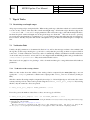
Thus, after the running muse_bias, the current working directory contains now the master bias product stored
in a single FITS file with 72 FITS extensions:
1> ls -1 *.fits
MASTER_BIAS.fits
Without the option “--merge” the recipe would have produced 24 FITS files with 3 FITS extensions each,
where the IFU from which it has been created is indicated by the 2 digit sequence number at the end of the file
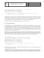
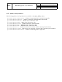
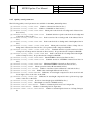
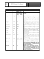
name (e.g. the MASTER_BIAS of IFU 1 would be stored in the file MASTER_BIAS-01.fits).
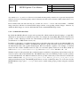
An example of a MUSE master bias is shown in Figure 6.1. For the full description of the muse_bias recipe
please refer to Section 9.
6.3.2
Dark
In this next step a set of raw dark frames is combined into a master dark frame using the recipe muse_dark.
Since the dark current of the MUSE CCDs is small, it is unlikely that the master dark frame will be needed in
the following processing steps. Thus this step is optional.
Following the same procedure as before, the set-of-frames is prepared containing at least 3 raw dark frames, and
the 24 master bias files from the previous processing step which are the required calibrations. Assuming the
master bias files are located in a directory $MUSE_CAL the SOF and the EsoRex command will look as shown
here:
7 Note that in parallel mode the messages written to the terminal and/or the log-file may not appear in order but interlaced depending
on the execution order of the different threads, which, in general, is not predictable.
8 i.e. if EsoRex is executed with the option “--suppress-prefix=true”; which is the built-in default setting.
ESO
MUSE Pipeline User Manual
Doc:
Issue:
Date:
Page:
VLT-MAN-ESO-14670-6186
Issue 9
Date 2015-04-28
35 of 132
Figure 6.1: Example of a MUSE master bias of a single IFU (channel 1), as it is created by the recipe muse_bias.
1> cat dark.sof
/data/muse/raw/dark/MUSE.2014-02-11T20:32:24.014.fits DARK
/data/muse/raw/dark/MUSE.2014-02-11T20:33:31.876.fits DARK
/data/muse/raw/dark/MUSE.2014-02-11T20:34:31.876.fits DARK
$MUSE_CAL/MASTER_BIAS.fits MASTER_BIAS
2> OMP_NUM_THREADS=24 esorex --log-file=dark.log muse_dark --nifu=-1 \
--merge dark.sof
The result of this EsoRex command is the master dark frame stored as a single FITS file with 72 FITS extensions.
FITS files:
1> ls -1 *.fits
MASTER_DARK.fits
ESO
MUSE Pipeline User Manual
Doc:
Issue:
Date:
Page:
VLT-MAN-ESO-14670-6186
Issue 9
Date 2015-04-28
36 of 132
In the following processing steps, the master dark will not be used. For the full description of the muse_dark
recipe please refer to Section 9.
6.3.3
Flat Field
In this processing step the recipe muse_flat is used to combine raw (lamp) flat field frames into a master flat
frame. In addition to that the slices are located on the image, and their edges are traced along the wavelength
axis (vertical axis). Finally bright and dark pixels are located.
The set-of-frames must contain at least 3 raw flat field frames and the master bias frame. Optionally the master
dark frame may added too, but it has been omitted in the following. The optional bad pixel table has been
used in the following example. However note that the use of a bad pixel table may actually degrade the tracing
solution if it contains bad columns, in particular if they are located near the edge of a slice.
1> cat flat.sof
/data/muse/raw/flat/MUSE.2014-02-21T12:14:59.316.fits
/data/muse/raw/flat/MUSE.2014-02-21T12:16:25.212.fits
/data/muse/raw/flat/MUSE.2014-02-21T12:18:10.540.fits
/data/muse/raw/flat/MUSE.2014-02-21T12:19:34.837.fits
/data/muse/raw/flat/MUSE.2014-02-21T12:20:48.296.fits
$MUSE_CAL/MASTER_BIAS.fits MASTER_BIAS
$MUSE_CAL/badpix_table.fits BADPIX_TABLE
FLAT
FLAT
FLAT
FLAT
FLAT
2> OMP_NUM_THREADS=24 esorex --log-file=flat.log muse_flat --nifu=-1 \
--merge flat.sof
The products of this EsoRex command are the master flat frame and the trace tables, each of them stored as
single FITS files containing the master flat field and the tracing solution for all IFUs respectively:
1> ls -1 *.fits
MASTER_FLAT.fits
TRACE_TABLE.fits
An example of a MUSE master flat is shown in Figure 6.2. For the full description of the muse_flat recipe
please refer to Section 9.
6.3.4
Wavelength Calibration
In this processing step the wavelength solution for each IFU is created using the recipe muse_wavecal. To
create the dispersion solution the recipe needs at least three raw arc-lamp frame as input. One raw frame for
each available arc-lamp. It is possible to use more than one of these sets as input.
These sets of three arc-lamp frames are created by the MUSE calibration template and therefore the a complete
set should always be available. In addition, this can be verified by looking at the FITS header keywords indicating the lamp shutter status INS.SHUT3.ST, INS.SHUT4.ST, and INS.SHUT5.ST9 . Only one of the
9 To verify that the lamps a actually active the keywords INS.LAMP3.ST, INS.LAMP4.ST, and INS.LAMP5.ST should be
checked.
ESO
MUSE Pipeline User Manual
Doc:
Issue:
Date:
Page:
VLT-MAN-ESO-14670-6186
Issue 9
Date 2015-04-28
37 of 132
Figure 6.2: Example of a MUSE master flat field of a single IFU (channel 1), as it is created by the recipe muse_flat.
keywords should indicate an open lamp shutter for a single arc-lamp frame, and for a complete input set one
needs 3 such arc-lamp frames, one for each shutter.
Dark correction and flat field correction will be applied if the master dark frame and the master flat field frame
are present in the set-of-frames respectrively. However applying the two corrections is not needed for the arclamp frames, and thus the input data for these correction are omitted in the set-of-frames shown in the following.
What is needed from the previous processing steps are the trace tables and the master bias frame, and from the
static calibrations the line catalog is required. The set-of-frames and the EsoRex command line to create the
wavelength solution are shown here:
1> cat wavecal.sof
/data/muse/raw/wave/MUSE.2014-02-19T10:58:29.838.fits ARC
/data/muse/raw/wave/MUSE.2014-02-19T11:00:03.593.fits ARC
ESO
MUSE Pipeline User Manual
Doc:
Issue:
Date:
Page:
VLT-MAN-ESO-14670-6186
Issue 9
Date 2015-04-28
38 of 132
/data/muse/raw/wave/MUSE.2014-02-19T11:02:10.205.fits ARC
$MUSE_CAL/MASTER_BIAS.fits MASTER_BIAS
$MUSE_CAL/TRACE_TABLE.fits TRACE_TABLE
$MUSE_CAL/line_catalog.fits LINE_CATALOG
2> OMP_NUM_THREADS=24 esorex --log-file=wavecal.log muse_wavecal --nifu=-1 \
--resample --residuals --merge wavecal.sof
The primary product created by this command is the wavelength solution. In addition to the primary product the
shown EsoRex command also creates for each IFU a product file with the fit residuals of the arc-lines, reduced
arc-lamp images (for each lamp separately and a combined one), and a resampled arc-lamp image which can be
used for a visual inspection of the wavelength solution. An example is shown in Figure 6.3.
For the full description of the muse_wavecal recipe please refer to Section 9.
6.3.5
Line Spread Function
For the subtraction of the sky background in the later steps of the processing of MUSE observations a representation of the MUSE line-spread function (LSF) is needed. The line-spread function can be calculated using the
recipe muse_lsf which computes the slice and wavelength dependent LSF from a set of arc-lamp spectra. The
recipe takes the same set of arc-lamp exposures as it is used with the muse_wavecal recipe. But, in order to
measure the faint wings of the line-spread function with a reasonable signal-to-noise ratio at least 10 arc-lamp
exposures for each arc-lamp should be used.
From the previous processing steps the recipe needs as input the wavelength solution, the trace table, and the
master bias, and from the static calibration the line catalog is needed. Optionally the bad pixel table, the master
dark, and the master flat field may be added to the input set-of-frames. The following example shows the
minimal contents of the set-of-frames and the EsoRex command to compute the line-spread function:
1> cat lsf.sof
/data/muse/raw/wave/MUSE.2014-02-19T10:58:29.838.fits ARC
/data/muse/raw/wave/MUSE.2014-02-19T11:00:03.593.fits ARC
/data/muse/raw/wave/MUSE.2014-02-19T11:02:10.205.fits ARC
$MUSE_CAL/MASTER_BIAS.fits MASTER_BIAS
$MUSE_CAL/TRACE_TABLE.fits TRACE_TABLE
$MUSE_CAL/WAVECAL_TABLE.fits WAVECAL_TABLE
$MUSE_CAL/line_catalog.fits LINE_CATALOG
2> OMP_NUM_THREADS=24 esorex --log-file=lsf.log muse_lsf --nifu=-1 \
--merge lsf.sof
The primary product of this EsoRex command is the lsf-profile, which is a stack of slice specific images of the
line-spread function for each IFU.
Generating an lsf-profile is computational heavy. Using a standard set of 5 exposures per arc-lamp the EsoRex
command shown before uses approximately 80 GB of memory and takes about 30 minutes. As an alternative to
creating the lsf-profile with muse_lsf, the lsf-profiles that come as part of the MUSE pipeline package could be
ESO
MUSE Pipeline User Manual
Doc:
Issue:
Date:
Page:
VLT-MAN-ESO-14670-6186
Issue 9
Date 2015-04-28
39 of 132
Figure 6.3: Example of a resampled arc-lamp frame of a single IFU (channel 1), as it is created by the recipe
muse_wavecal. This image is the result of combining the three individual arc-lamp images and applying the determined
wavelength solution. As it is expected from a good wavelength solution the arc-lines appear as straight, horizontal lines,
i.e. they are now on the same wavelength.
used in the following reduction steps. The analysis of MUSE commissioning data show that the parameters of
the line spread function are stable, so that a frequent update of the lsf-profile is not necessary.
For the full description of the muse_lsf recipe please refer to Section 9.
ESO
6.3.6
MUSE Pipeline User Manual
Doc:
Issue:
Date:
Page:
VLT-MAN-ESO-14670-6186
Issue 9
Date 2015-04-28
40 of 132
Instrument Geometry
The instrument geometry or geometrical calibration determines where in the field-of-view each slice of each
IFU is located. The result is the geometry table which can be created using the muse_geometry recipe.
However, this recipe requires special input data and some expert knowledge to get to a good result! For this
reason geometry tables are carefully prepared in advance. They are considered as a static calibration which is
distributed as part of the MUSE pipeline release package.
Therefore, an example and a description of the recipe muse_geometry is not shown here.
6.3.7
Illumination Correction
Twilight flats are part of the regular calibrations taken for MUSE. In this processing step the raw sky-flat frames
are combined into a three-dimensional illumination correction using the recipe muse_twilight10 . In addition
the created twilight-cube carries the integrated flux value on to the further processing steps, as an estimate of
the relative throughput of the IFUs.
The recipe needs as input at least 3 raw sky-flat frames, the master bias frame, the master flat field, the trace
table, the wavelength solution and the geometry table. The set-of-frames and the EsoRex command for creating
the master sky-flat are shown:
1> cat twilight.sof
/data/muse/raw/MUSE.2014-02-20T23:31:38.542.fits SKYFLAT
/data/muse/raw/MUSE.2014-02-20T23:33:49.258.fits SKYFLAT
/data/muse/raw/MUSE.2014-02-20T23:36:21.511.fits SKYFLAT
$MUSE_CAL/MASTER_BIAS.fits MASTER_BIAS
$MUSE_CAL/MASTER_FLAT.fits MASTER_FLAT
$MUSE_CAL/TRACE_TABLE.fits TRACE_TABLE
$MUSE_CAL/WAVECAL_TABLE.fits WAVECAL_TABLE
$MUSE_CAL/geometry_table.fits GEOMETRY_TABLE
$MUSE_CAL/vignetting_mask.fits VIGNETTING_MASK
2> OMP_NUM_THREADS=24 esorex --log-file=twilight.log muse_twilight twilight.sof
The vignetting mask is an optional input to the recipe and, if provided, is used to correct vignetted regions in
the MUSE field of view. Usually vignetting is present in the lower right corner of the MUSE field-of-view.
The primary product of this processing step is the twilight cube, which is a data cube of the smoothed twilight
sky. As an additional product the data cube created from the combined twilight images is available. It is the
data cube of the twilight sky before the smoothing is applied.
The recipe works on the data of all 24 IFUs simultaneously, in the same way as the post-processing recipes do.
Thus the recipe options --nifu and --merge are not applicable to this recipe.
For the full description of the muse_twilight recipe please refer to Section 9.
10 Since
version 1.0 the recipe muse_twilight replaces the recipe muse_skyflat
ESO
6.4
MUSE Pipeline User Manual
Doc:
Issue:
Date:
Page:
VLT-MAN-ESO-14670-6186
Issue 9
Date 2015-04-28
41 of 132
Observation Pre-processing
At this point all necessary calibrations have been created to remove the instrument signature from the on-sky
exposures using the pre-processing recipe muse_scibasic. This also converts the observations to the pixel table
format which is the input format for the post-processing recipes. During this conversion sky lines are used to
correct for offsets in the wavelength solution and, optionally, the data is corrected for the relative illumination
of the slices for individual IFUs.
Pixel tables can be saved as FITS images or as a true FITS binary tables. To benefit from the more efficient
way to read and write FITS images the results are, by default saved using the FITS image based format11 . If
the pixel tables should be stored a FITS binary tables, then this can be done by setting the environment variable
MUSE_PIXTABLE_SAVE_AS_TABLE=1.
In the example the usage of muse_scibasic is shown for a scientific exposure as input (i.e. for the raw frame tag
OBJECT). But it has to be applied in the same way to the observations of standard stars, astrometric fields and
empty sky fields (i.e. the raw frame tags STD, ASTROMETRY, and SKY).
For each of these four types of observations the recipe takes one or more raw exposures as input. The required
calibrations are master bias, master flat, trace table, wavelength solution and the geometry table. Optionally a
master sky-flat and a bad pixel table may be used. The resulting set-of-frames and the EsoRex command to run
muse_scibasic are shown here:
1> cat object.sof
/data/muse/raw/object/MUSE.2014-08-04T09:34:48.604.fits OBJECT
/data/muse/raw/object/MUSE.2014-08-04T09:32:59.174.fits ILLUM
$MUSE_CAL/MASTER_BIAS.fits MASTER_BIAS
$MUSE_CAL/MASTER_FLAT.fits MASTER_FLAT
$MUSE_CAL/TWILIGHT_CUBE.fits TWILIGHT_CUBE
$MUSE_CAL/TRACE_TABLE.fits TRACE_TABLE
$MUSE_CAL/WAVECAL_TABLE.fits WAVECAL_TABLE
$MUSE_CAL/badpix_table.fits BADPIX_TABLE
$MUSE_CAL/geometry_table.fits GEOMETRY_TABLE
2> OMP_NUM_THREADS=24 esorex --log-file=object.log muse_scibasic --nifu=-1 \
--merge object.sof
Optionally the recipe muse_scibasic takes an illumination flat field (frame tag ILLUM), as shown in the example.
This flat field, is a special raw continuum lamp exposure illuminating the whole field-of-view. It is taken
regularly during the night, at a rate of 1 exposure every 1–2 hours, as part of the instrument calibration plan. It
can be added to the set-of-frames as shown in the example. If it is present the recipe muse_scibasic corrects
for the relative illumination of the slices on a per IFU basis (temperature dependent illumination changes).
The command shown before creates the pixel table stored as 24 FITS files for each input exposure, and one
reduced image.
1> ls -1 *.fits
OBJECT_RED_0001.fits
11 With
version 1.0 the default format has been changed to FITS images
ESO
MUSE Pipeline User Manual
Doc:
Issue:
Date:
Page:
VLT-MAN-ESO-14670-6186
Issue 9
Date 2015-04-28
42 of 132
PIXTABLE_OBJECT_0001-01.fits
...
PIXTABLE_OBJECT_0001-24.fits
Currently the option -merge affects only the products which are not pixel tables, i.e. the reduced images,
which may be used for a visual check of the applied corrections. On the other hand these reduced images are
usually not needed, and using the recipe option --saveimage=FALSE they are not created at all.
The product file names are derived from the frame tag of the raw input exposure, which, in this case, was
“OBJECT”. For the other kind of on-sky exposures the product files are named in the same way but with the
OBJECT-part replaced by the corresponding frame tag.
The 4 digit number indicates the index of the input exposure, which in this case is always “0001” since there
was only a single raw science exposure present in the SOF. If more than one raw exposure is present the index
will run from 1 to the number of exposures.
The full description of the muse_scibasic recipe can be found in Section 9.
6.5
Observation Post-Processing
This section covers the second stage of the MUSE data reduction cascade shown in Figure 2.3. Again the processing steps are executed from left to right, although only the response computation is mandatory for creating
the final data cube.
6.5.1
Flux Calibration
In this first processing step the response curve for the flux calibration of the science observations is created from
a pre-processed standard star observation. The raw standard star observation has already been processed with
muse_scibasic and resulting 24 pixel tables are now located in the current working directory.
In addition to the set of 24 pixel tables, the recipe requires an exintion table, and a standard flux table. Optionally
a list of predefined telluric regions may be present in the input SOF (which is omitted in the following).
The standard flux table is a catalog of reference spectra of spectrophotometric standard stars. The current
version of this catalog, which is included in the MUSE pipeline distribution as std_flux_table.fits, will
eventually contain spectra of all spectrophotometric standard stars which are regularly observed with MUSE.
The standard stars in the standard flux table are looked up by their coordinates.
Currently reference spectra for the following standard stars are available:
• GD71
• GD108
• GD153
• HD49798
• CD-32 9927 (bad resolution, should not be used!)
ESO
MUSE Pipeline User Manual
Doc:
Issue:
Date:
Page:
VLT-MAN-ESO-14670-6186
Issue 9
Date 2015-04-28
43 of 132
• GJ 754.1 A
• LDS 749B
• Feige 110
• LTT 7987
• EG 274
• LTT 3218
The complete set-of-frames for computing the response curve is shown here, followed by the EsoRex command
line to launch the recipe.
1> cat std.sof
PIXTABLE_STD_0001-01.fits PIXTABLE_STD
...
PIXTABLE_STD_0001-24.fits PIXTABLE_STD
$MUSE_CAL/extinct_table.fits EXTINCT_TABLE
$MUSE_CAL/std_flux_table.fits STD_FLUX_TABLE
2> OMP_NUM_THREADS=24 esorex --log-file=std.log muse_standard \
--filter=white std.sof
The recipe creates a data cube of the standard star observation, and the response curve and the telluric correction
spectrum.
1> ls -1 *.fits
DATACUBE_STD_0001.fits
STD_RESPONSE_0001.fits
STD_TELLURIC_0001.fits
Again the sequence number is an exposure index, which runs from 1 to the number of exposures present in the
SOF.
The data cube can be visualized using the ESO 3D Visualization tool (cf. RD[7], Section E) or ds9 for instance.
In addition to the data cube itself, the data cube product file contains a reconstructed FOV image for each filter
given on the command line (option --filter). The default filter setting is “white” to produce a white light
image. All other allowed filters are the ones defined in the filter list calibration file (filter_list.fits;
the filter names are given by the keyword EXTNAME). If a filter from the filter list is chosen the filter list must
also be present in the SOF.
By default the recipe selects the brightest star in the field as the spectro photometric standard. If this is inappropriate for the current observation, this can be changed using the recipe option --select=distance, which
then takes the object closest to the expected position.
If more than one standard star observation is present in the input SOF the response computation is done separately for each of the input exposures.
For the full description of the muse_standard recipe please refer to Section 9.
ESO
6.5.2
MUSE Pipeline User Manual
Doc:
Issue:
Date:
Page:
VLT-MAN-ESO-14670-6186
Issue 9
Date 2015-04-28
44 of 132
Sky Creation
In this processing step a model of the sky spectrum is created using the recipe muse_create_sky. It is only
needed if the observed object fills the field-of-view to such an extent that a reasonable sky spectrum cannot
obtained directly on the observation itself. Otherwise, if the science exposure contains enough sky, the sky
subtraction can be done directly when the science exposure is processed.
The recipe requires that exposure(s) of a mostly empty sky field are available and have been pre-processed as
shown in Section 6.4. It also recommended use an lsf-profile which has been created during the basic reduction,
or is taken from the static calibrations. The lsf-profile contains a model of the slice and wavelength dependent
MUSE line-spread function which is used to create a smooth sky continuum model by subtracting the fitted sky
lines from the full sky spectrum.
The required calibrations are the list of sky lines, the extinction table and the response curve, and, optionally,
the telluric correction. The input set-of-frames, and the EsoRex command line to run muse_create_sky using
default settings are shown:
1> cat sky.sof
PIXTABLE_SKY_0001-01.fits PIXTABLE_SKY
...
PIXTABLE_SKY_0001-24.fits PIXTABLE_SKY
$MUSE_CAL/LSF_PROFILE.fits LSF_PROFILE
$MUSE_CAL/STD_RESPONSE_0001.fits STD_RESPONSE
$MUSE_CAL/STD_TELLURIC_0001.fits STD_TELLURIC
$MUSE_CAL/extinct_table.fits EXTINCT_TABLE
$MUSE_CAL/sky_lines.fits SKY_LINES
2> OMP_NUM_THREADS=24 esorex --log-file=sky.log muse_create_sky \
sky.sof
The result of the above command are the products
1> ls -1 *.fits
IMAGE_FOV.fits
SKY_CONTINUUM.fits
SKY_LINES.fits
SKY_MASK.fits
SKY_SPECTRUM.fits
These are the reconstructed whitelight field-of-view image, the estimated sky continuum spectrum, estimated
fluxes of the sky lines, image mask of the sky regions derived from the white light image, and the sky spectrum
obtained from the sky regions defined by the mask.
Note that the sky continuum is always created, even if no lsf-profile is present in the input SOF. However, a
reasonably smooth version of the sky continuum will only be obtained if an lsf-profile is used.
For the full description of the muse_create_sky recipe please refer to Section 9.
ESO
6.5.3
MUSE Pipeline User Manual
Doc:
Issue:
Date:
Page:
VLT-MAN-ESO-14670-6186
Issue 9
Date 2015-04-28
45 of 132
Astrometry
This processing step uses muse_astrometry to create the astrometric calibration from the pre-processed pixel
tables of an exposure of an astrometric field. The obtained astrometric calibration is needed to create the world
coordinate system for the science exposure and assign right ascension and declination to the spaxels of the data
cube.
In addition to the input pixel tables the recipe needs an astrometric reference catalog. The astrometric catalog
that comes with the MUSE pipeline distribution will eventually contain the positions of the reference stars in all
astrometric fields which are regularly observed with MUSE. Currently the distributed catalog includes 11 fields
of the 6 globular clusters.
Optionally the extinction table, a response curve, and a telluric correction may be present in the input set-offrames. If the optional calibrations are present, the corresponding corrections are performed before the reference
objects are identified and the WCS solution is computed. However, experience shows that the improvement that
can be achieved by using the optional calibrations is very limited, if it is present at all.
The following shows the input set-of-frames and the EsoRex command to create the WCS solution:
1> cat astrometry.sof
PIXTABLE_ASTROMETRY_0001-01.fits PIXTABLE_ASTROMETRY
...
PIXTABLE_ASTROMETRY_0001-24.fits PIXTABLE_ASTROMETRY
$MUSE_CAL/STD_RESPONSE_0001.fits STD_RESPONSE
$MUSE_CAL/STD_TELLURIC_0001.fits STD_TELLURIC
$MUSE_CAL/extinct_table.fits EXTINCT_TABLE
$MUSE_CAL/astrometry_reference.fits ASTROMETRY_REFERENCE
2> OMP_NUM_THREADS=24 esorex --log-file=astrometry.log muse_astrometry \
astrometry.sof
The results are the data cube and the computes WCS solution:
1> ls -1 *.fits
ASTROMETRY_WCS_0001.fits
DATACUBE_ASTROMETRY_0001.fits
It is necessary to always use an astrometric solution together with the geometry table that has been used to
compute it. The reason for this is that the astrometric solution may compensate for small inaccuracies in the
geometry table, so that a specific astrometric solution should always be used in pairs with its matching geometry
table.
The pipeline distribution comes with a carefully verified WCS solution as a master calibration, which matches
the geometry table that comes with the pipeline distribution. Also, since the WCS solution was found to be
stable when analyzing the available commissioning data, there is no need to recreate the astrometric calibration,
and this step may safely be skipped.
For the full description of the muse_astrometry recipe please refer to Section 9.
ESO
6.5.4
MUSE Pipeline User Manual
Doc:
Issue:
Date:
Page:
VLT-MAN-ESO-14670-6186
Issue 9
Date 2015-04-28
46 of 132
Science Observations
At this point all calibrations are in place and one can start with the post-processing of the science observations
using muse_scipost. The recipes applies the previously created on-sky calibrations and creates the final data
cube from the pre-processed pixel tables of scientific observations.
In the following example a full data cube is created from a single exposure, the sky background is removed
and the flux calibration and the astrometric calibration, created in the preceding processing steps, are applied.
Finally four field-of-view images are created from the data cube, each of them covering the wavelength band of
one of the filters given on the command line.
Thus, the input set-of-frames will contain the 24 pre-processed pixel tables of the exposure of the science
target, the estimated fluxes of the sky lines, the response curve, the telluric correction, the extinction table, the
astrometric calibration, and the list of filter transmission curves.
Note: The astrometric calibration to be used here should be created from the the same geometry table as the
input pixel tables (see Section 6.5.3 for details).
The input set-of-frames and the EsoRex command to run muse_scipost are show in the following. Note that, depending on the orientation of the original scientific exposure (cf. Section 3.1), this command will need between
approximately 18 GB and 25 GB of RAM in order finish sucessfully.
1> cat scipost.sof
PIXTABLE_OBJECT_0001-01.fits PIXTABLE_OBJECT
...
PIXTABLE_OBJECT_0001-24.fits PIXTABLE_OBJECT
$MUSE_CAL/LSF_PROFILE.fits LSF_PROFILE
$MUSE_CAL/STD_RESPONSE_0001.fits STD_RESPONSE
$MUSE_CAL/STD_TELLURIC_0001.fits STD_TELLURIC
$MUSE_CAL/ASTROMETRY_WCS_0001.fits ASTROMETRY_WCS
$MUSE_CAL/sky_lines.fits SKY_LINES
$MUSE_CAL/extinct_table.fits EXTINCT_TABLE
$MUSE_CAL/filter_list.fits FILTER_LIST
2> OMP_NUM_THREADS=24 esorex --log-file=scipost.log muse_scipost \
--filter=white,Johnson_V,Cousins_R,Cousins_I scipost.sof
The product files created by this command are:
1> ls -1 *.fits
DATACUBE_FINAL.fits
IMAGE_FOV_0001.fits
IMAGE_FOV_0002.fits
IMAGE_FOV_0003.fits
IMAGE_FOV_0004.fits
The 4 digit sequence number of the created field-of-view images refers to the different filters. The “ordering”
of the field-of-view images corresponds to the order of the filters on the command line.
By default the recipe performs a model based sky subtraction, i.e. initially a model of the sky lines and the sky
continuum are computed using the darkest regions in the field-of view, and then these models are subtracted
ESO
MUSE Pipeline User Manual
Doc:
Issue:
Date:
Page:
VLT-MAN-ESO-14670-6186
Issue 9
Date 2015-04-28
47 of 132
from the data. To use the models obtained from a previous run of muse_create_sky one can change the sky
subtraction method using the option --skymethod. If this option is set to subtract-model the input
models of the sky lines and the sky continuum are subtracted from the observation data as they are.
As mentioned before, running muse_scipost to process a single exposure requires already a quite capable computer (in terms of memory). And, contrary to the basic calibration recipe reducing the number of threads will
not reduce the memory needed. It is also not possible to process an observation by splitting it into smaller tiles.
However, it is possible to limit the wavelength range to process using the recipe options --lambdamin and
--lambdamax, which will reduce the memory usage (cf. Section 7.1).
The recipe muse_scipost accepts the pixel tables of more than one exposure as input. In this case the exposures
will be combined into a single data cube by default. However, in order to obtain the expected results when
combining exposures read Section 6.6 first!
As long as single science exposures are concerned, the data processing has finished at this point and one can
start with the scientific analysis of the data.
For the full description of the muse_scipost recipe please refer to Section 9.
6.6
Combining Exposures
This section shows how multiple exposures are combined efficiently and correctly, and should help to bypass
some pitfalls. The combination of exposures, i.e. the combination of the pre-processed pixel tables of a scientific exposure can be done with two different methods (recipes). The exposures can be combined directly in
muse_scipost, or one can use the utility recipe muse_exp_combine. The latter uses a fully reduced pixel table,
which is an intermediate product of muse_scipost.
There are two issues which have to be considered when multiple exposures are combined, the correction of
coordinate offsets, and limiting the wavelength range.
6.6.1
Correcting Coordinate Offsets
When combining multiple exposures, the pipeline recipes muse_scipost and muse_exp_combine usually do a
good job to automatically recover the relative offsets from the information in the FITS header of each exposure,
provided that two conditions are met:
1. the same VLT guide star was used to observe all exposures,
2. the exposures were all taken at the same position angle.
Since MUSE exposures are often observed using a dither pattern that involves 90◦ rotations, condition 2 is often
not true, and the user has to provide offset corrections to the pipeline.12 The reference may be some external data
or one of the exposures itself. For instance, the reconstructed field-of-view images may be used for measuring
the coordinate offsets (creating these images can be done quickly with muse_scipost using a vary narrow range
in wavelength).
12 This is due to a slight decentering of the axis of the derotator, leading to a "derotator wobble". Future versions of the pipeline should
be able to automatically correct this effect.
ESO
MUSE Pipeline User Manual
Doc:
Issue:
Date:
Page:
VLT-MAN-ESO-14670-6186
Issue 9
Date 2015-04-28
48 of 132
The offset corrections can then be applied in two ways:
1. Edit the FITS headers:
Before starting muse_scipost or muse_exp_combine to create a combined cube, edit the main FITS
headers of the input pixel tables and replace the RA and DEC header keywords with corrected values that
are measured externally.
2. Provide offsets:
The coordinate offsets are given by setting the environment variables MUSE_XCOMBINE_RA_OFFSETS
and MUSE_XCOMBINE_DEC_OFFSETS. Each of these variables has to contain as many floating-point
numbers, separated by commas, as exposures to combine are involved.
Each number is the direct difference of the measured position to the reference position (no cos δ !), the
values are interpreted in units of degrees:
RA_OFFSET = RAmeasured − RAreference
DEC_OFFSET = DECmeasured − DECreference
It is important that the offsets are given in the order of increasing DATE-OBS of the exposures involved.
If one of the exposures has been chosen as the reference the offsets of 0 for this exposure have to be
explicitly given when setting the environment variables.
6.6.2
Limiting Wavelength Ranges
All recipes reading pixel tables support the --lambdamin and --lambdamax recipe parameters to restrict
the wavelength range they are working on. These recipe parameters expect a wavelength given in Angstrom,
and this can be used to limit the amount of memory required by the recipes (see Section 7.1 for details).
For the combination of exposures the limiting factor in terms of memory is the size of the output data cube,
which has to be constructed in memory. Thus, in limiting the wavelength range the output data cube can cover
a larger area on the sky.
6.6.3
Combining Exposures using muse_scipost
The following example shows how three exposures are combined using muse_scipost alone. The input set-offrames now contains the pixel tables of the three exposures (note the 4-digit index in the names of the pixel
tables). Apart from the additional pixel tables the set-of-frames is identical to the one shown previously for
processing a single exposure.
The EsoRex command line shows the three coordinate offsets for the 3 input exposures where the first exposure
is used as the coordinate reference. The wavelength range is restricted to the intervall 6900 Å to 7100 Å.
1> cat scipost_combine.sof
PIXTABLE_OBJECT_0001-01.fits PIXTABLE_OBJECT
...
ESO
MUSE Pipeline User Manual
Doc:
Issue:
Date:
Page:
VLT-MAN-ESO-14670-6186
Issue 9
Date 2015-04-28
49 of 132
PIXTABLE_OBJECT_0001-24.fits PIXTABLE_OBJECT
PIXTABLE_OBJECT_0002-01.fits PIXTABLE_OBJECT
...
PIXTABLE_OBJECT_0002-24.fits PIXTABLE_OBJECT
PIXTABLE_OBJECT_0003-01.fits PIXTABLE_OBJECT
...
PIXTABLE_OBJECT_0003-24.fits PIXTABLE_OBJECT
$MUSE_CAL/LSF_PROFILE.fits LSF_PROFILE
$MUSE_CAL/STD_RESPONSE_0001.fits STD_RESPONSE
$MUSE_CAL/STD_TELLURIC_0001.fits STD_TELLURIC
$MUSE_CAL/ASTROMETRY_WCS_0001.fits ASTROMETRY_WCS
$MUSE_CAL/sky_lines.fits SKY_LINES
$MUSE_CAL/extinct_table.fits EXTINCT_TABLE
$MUSE_CAL/filter_list.fits FILTER_LIST
2> OMP_NUM_THREADS=24 \
MUSE_XCOMBINE_RA_OFFSETS="0.0000000,-5.4920943e-05,-0.00031381379" \
MUSE_XCOMBINE_DEC_OFFSETS="0.0000000,8.3338105e-05,7.2223397e-05" \
esorex --log-file=scipost_combine.log muse_scipost \
--lambdamin=6900. --lambdamax=7100. scipost_combine.sof
The product files created by this command are:
1> ls -1 *.fits
DATACUBE_FINAL.fits
IMAGE_FOV_0001.fits
The final data cube covers the combined field-of-view of the individual input exposures, but only the small
wavelength band defined by the recipe parameters. By default the recipe muse_scipost creates a white light
field-of-view image, which in the above case covers only the limited wavelength range.
6.6.4
Combining Exposures using muse_exp_combine
With the previous method, one has to re-run the full science post-processing in order to get the data cubes for a
different wavelength band or combination of input fields. A slightly more flexible approach is shown here.
Assuming that the computer used to run muse_scipost is capable of processing a single exposure without restricting the wavelength range. In this case one can create a fully reduced pixel table for the first exposure using
the following EsoRex command:
1> cat scipost_1.sof
PIXTABLE_OBJECT_0001-01.fits PIXTABLE_OBJECT
...
PIXTABLE_OBJECT_0001-24.fits PIXTABLE_OBJECT
$MUSE_CAL/LSF_PROFILE.fits LSF_PROFILE
$MUSE_CAL/STD_RESPONSE_0001.fits STD_RESPONSE
$MUSE_CAL/STD_TELLURIC_0001.fits STD_TELLURIC
$MUSE_CAL/ASTROMETRY_WCS_0001.fits ASTROMETRY_WCS
ESO
MUSE Pipeline User Manual
Doc:
Issue:
Date:
Page:
VLT-MAN-ESO-14670-6186
Issue 9
Date 2015-04-28
50 of 132
$MUSE_CAL/sky_lines.fits SKY_LINES
$MUSE_CAL/extinct_table.fits EXTINCT_TABLE
$MUSE_CAL/filter_list.fits FILTER_LIST
2> OMP_NUM_THREADS=24 esorex --log-file=scipost_1.log muse_scipost \
--save=individual scipost_1.sof
The product files created by this commands are:
1> ls -1 *.fits
DATACUBE_FINAL_0001.fits
IMAGE_FOV_0001.fits
PIXTABLE_REDUCED_0001.fits
which are then renamed to prevent overwriting them with the EsoRex calls needed to process the remaining
exposures:
1> mv DATACUBE_FINAL.fits DATACUBE_FINAL_EXP01.fits
2> mv IMAGE_FOV_0001.fits IMAGE_FOV_0001_EXP01.fits
3> mv PIXTABLE_REDUCED_0001.fits PIXTABLE_REDUCED_0001_EXP01.fits
By using the recipe parameter --save_individual a fully reduced pixel table is created as an additional
product. Fully reduced means that all on-sky calibrations have been applied, and the only processing step
missing is the resampling into the final data cube.
Proceeding in the same way with the other exposures one finally ends up with one fully reduced pixel table for
each exposure. These can now be used as input for the recipe muse_exp_combine to create a final, combined
data cube. The advantage is that creating cubes for different wavelength bands or combination of the exposures
now involves only the resampling step.
To get to the same final data cube as in the previous section, the command to be issued is:
1> cat exp_combine.sof
PIXTABLE_REDUCED_0001_EXP01.fits PIXTABLE_REDUCED
PIXTABLE_REDUCED_0001_EXP02.fits PIXTABLE_REDUCED
PIXTABLE_REDUCED_0001_EXP03.fits PIXTABLE_REDUCED
$MUSE_CAL/filter_list.fits FILTER_LIST
2> OMP_NUM_THREADS=24 \
MUSE_XCOMBINE_RA_OFFSETS="0.0000000,-5.4920943e-05,-0.00031381379" \
MUSE_XCOMBINE_DEC_OFFSETS="0.0000000,8.3338105e-05,7.2223397e-05" \
esorex --log-file=exp_combine.log muse_exp_combine \
--lambdamin=6900. --lambdamax=7100. exp_combine.sof
The product files created by this command are:
1> ls -1 *.fits
DATACUBE_FINAL.fits
IMAGE_FOV_0001.fits
ESO
MUSE Pipeline User Manual
Doc:
Issue:
Date:
Page:
VLT-MAN-ESO-14670-6186
Issue 9
Date 2015-04-28
51 of 132
And finally, there are also other scenarios where combining the fully reduced pixel tables using the recipe
muse_exp_combine is useful. For instance when science observations, which are accompanied by dedicated
sky observations, should be combined. In this case each of science observations has to be calibrated separately
using the corresponding sky observation. After this is done the fully reduced science observations can be
combined with muse_exp_combine.
ESO
7
MUSE Pipeline User Manual
Doc:
Issue:
Date:
Page:
VLT-MAN-ESO-14670-6186
Issue 9
Date 2015-04-28
52 of 132
Tips & Tricks
7.1
Restricting wavelength ranges
All post-processing recipes read pixel tables. When testing such steps of the data reduction, it can be benificial
to work on only a subset of the data, like a small wavelength range. All relevant recipes therefore support the
--lambdamin and --lambdamax recipe parameters. This causes the code to still read the full pixel tables,
but then the pixels with wavelengths not in the given range are discarded.13 This can be used to speed up
processing and constrain memory consumption, e.g. to test parameter ranges that affect the cube reconstruction.
Note, however, that they may have unforeseen consequences if e.g. the data are truncated right on a bright sky
line.
7.2
Verification Tools
Usually, the QC parameters as documented in Section 9 as well as the messages written to the terminal (and
the log-file) by the recipe should give a good basis to verify that the processing worked as expected. But in
some cases, a visual verification is necessary, and tools which help with the visualization and the verification
of the results may be needed. A few such tools are shipped with the MUSE pipeline and get installed into
<installation prefix>/bin. They are described in this section.
The visual tools use gnuplot14 for plotting15 . All tools mentioned here give a usage hint when called without
parameters.
7.2.1
Verification of the tracing solution
When one has doubts about the validity of the tracing solution computed by the muse_flat recipe, one can
specify the --samples parameter so that the extra output product TRACE_SAMPLES is written (one file per
IFU).
This file contains all tracing samples computed by the recipe, i.e. left and right edge as well as the slice center
at many vertical positions. These can be plotted using the tool muse_trace_plot_samples. If just using
this file, only the central two slices are plotted:
1> muse_trace_plot_samples TRACE_SAMPLES-06.fits
If one also passes the number of the slices to show, one can e.g. plot all slices:
1> muse_trace_plot_samples -s1 1 -s2 48 TRACE_SAMPLES-06.fits
13 Since
the pixel tables are not and cannot be sorted, reading the full tables is necessary. It causes a temporary peak in memory usage
to at least the size of the pixel table.
14 Available from http://www.gnuplot.info/.
15 The plots can hence be customized in the same way as other gnuplot-based scripts.
One can use e.g. using the file
$HOME/.gnuplot to set up the preferred terminal type or cause gnuplot to write to a file instead of displaying a window.
ESO
MUSE Pipeline User Manual
Doc:
Issue:
Date:
Page:
VLT-MAN-ESO-14670-6186
Issue 9
Date 2015-04-28
53 of 132
Figure 7.1: The graphical window showing the output of the muse_trace_plot_samples tool, then plotting slices
12 to 20 in IFU 6, using the trace samples table, the trace table, and the master flat-field image (see text for details).
Tip: when the default gnuplot setup is used (with the x11, wxt, or qt "terminals"), one can use the right mouse
button on the plot window to zoom the display to a rectangular region.
When also passing the tracing table on the command line, the tool plots the polynomial solutions for both edges
and the center over the crosses that mark the sampling points:
1> muse_trace_plot_samples -s1 1 -s2 48 TRACE_SAMPLES-06.fits TRACE_TABLE-06.fits
Here, one has to be careful to select files that belong to the same IFU! Then one can visually verify that the
polynomial solution matches the individual traced points.
Finally, one can also use the master flat-field product as background of the plot, so that one can actually check
that the tracing points were correctly computed:
1> muse_trace_plot_samples -s1 12 -s2 20 TRACE_SAMPLES-06.fits \
TRACE_TABLE-06.fits MASTER_FLAT-06.fits
ESO
MUSE Pipeline User Manual
Doc:
Issue:
Date:
Page:
VLT-MAN-ESO-14670-6186
Issue 9
Date 2015-04-28
54 of 132
Figure 7.2: The graphical window showing the output of the muse_trace_plot_widths tool, plotting slices 1 to 48
of IFU 6, using the trace samples table (see text for details).
Plotting this may take a while, so it’s advisable to only use a subset of the slices. The result of this command is
shown in Figure 7.1.
The widths of the slices on the CCD should be around 77 pixels, but their actual widths may slowly vary
between top and bottom of the CCD, and between the slices near the edges and in the center of the CCD. The
tool muse_trace_plot_widths was written to help to assess that there are no sudden jumps in the tracing.
When called with a tracing samples table, the samples of all slices are shown, as displayed in Figure 7.2. A
color gradient (from green on the left of the CCD to red on the right) plus different symbols are used to make
the slices distinguishable. It is apparent that the slices on the edges of the CCD are the widest (above 78 pix)
while those near the center of the CCD are narrow (below 76 pixels).
7.2.2
Verification of the wavelength solution
The tool muse_wave_plot_residuals can be used to verify the two-dimensional wavelength solution of
each slice or of all slices of one IFU. To use it one needs to run the muse_wavecal recipe with the --residuals
option, so that the extra product WAVECAL_RESIDUALS is created. Then one can run e.g.
1> muse_wave_plot_residuals WAVECAL_RESIDUALS-10.fits
and get a 2D map in CCD coordinates of the residuals of all the computed arc line centers with respect to the
final solution. This is displayed in Figure 7.3. There, one can see regions on the CCD that are not covered by
arc lines as white patches, and the points with the strongest blue and red colors give the strongest deviations
from the final solution. One can use the same command to change the vertical axis of the plot from CCD pixels
ESO
MUSE Pipeline User Manual
Doc:
Issue:
Date:
Page:
VLT-MAN-ESO-14670-6186
Issue 9
Date 2015-04-28
55 of 132
Figure 7.3: The graphical window showing the output of the muse_wave_plot_residuals tool, plotting all slices
of IFU 10, using the wavelength calibration residuals table (see text for details).
to wavelength, using the -l parameter:
1> muse_wave_plot_residuals -l WAVECAL_RESIDUALS-10.fits
In case one wants to look at only one slice, one can use the -s parameter with a slice number; color cuts are
adjustable using the -c parameter with two numbers, and one can study a different iteration (by default, the
final iteration of the fit in each slice is selected), using -i and a positive integer.
For a more in detail inspection of the solution of a single slice, one can use the muse_wave_plot_column
tool. This needs both the wavelength calibration table and the table with the residuals (make sure to use the
tables of the same recipe run and IFU!). It can be used on the data of a single slice (parameter -s) or on a single
CCD column (-c). It is most useful when displaying the vertical axis as residuals, using -r. Figure 7.4 shows
the output of the command
1> muse_wave_plot_column -s 12 -r WAVECAL_TABLE-10.fits WAVECAL_RESIDUALS-10.fits
This is an example of a good calibration with low residuals (the final RMS for the solution in this slice was
0.030 Å). The tool has automatically selected all columns belonging to this slice and colored them according to their horizontal position on the CCD (green is left, red is right), and used different symbols. As one
can see, the fainter arc lines (like the Ne I line at 5400.6 Å) have typically a much larger spread of residuals than the bright lines (e.g. Ne I at 6678.3 Å). With the default parameters of muse_wavecal (i.e. option
--fitweighting=cerrscatter) the weak lines are hence weighted much less in the fit of the wavelength solution than the bright lines.
ESO
MUSE Pipeline User Manual
Doc:
Issue:
Date:
Page:
VLT-MAN-ESO-14670-6186
Issue 9
Date 2015-04-28
56 of 132
Figure 7.4: The graphical window showing the output of the muse_wave_plot_column tool, plotting slice 12 of
IFU 10, using the wavelength calibration residuals and wavelength calibration tables (see text for details).
7.3
7.3.1
Miscellaneous Tools
Handling of MUSE pixel tables
MUSE pixel tables are heavily used as intermediate data products, and they have one special column that is not
easy to interpret (the "origin" column). Because of that a tool, muse_pixtable_dump, was added which
decodes these values and shows them in a readable form. One should always use the -c parameter to limit the
number of rows that are displayed, otherwise it might take very long to complete. One should also give the
starting row of the region that one is interested in, using -s:
1> muse_pixtable_dump -s 100000 -c 10 PIXTABLE_OBJECT_0001-01.fits
This command results in the output:
#
#
#
#
#
MUSE pixel table "PIXTABLE_OBJECT_0001-01.fits", showing 10 rows starting at index 100000 of 13514329
xpos
ypos
lambda
data
dq
stat
weight
exposure IFU xCCD yCCD xRaw yRaw slice
pix
pix Angstrom
(flux)
flag
(flux**2) ---------No
No
pix pix pix pix No
flux
in [count]
flux**2 in [count**2]
-78.72976685 -141.46130371 6346.222
1.35237e+01 0x00000000 1.62160e+01 0.0000e+00
0
1
47 1438
79 1470
1
-79.66138458 -141.48033142 6346.263
8.97605e+00 0x00000000 1.28346e+01 0.0000e+00
0
1
48 1438
80 1470
1
-80.59300232 -141.49934387 6346.304
1.71657e+01 0x00000000 1.90208e+01 0.0000e+00
0
1
49 1438
81 1470
1
-81.52462769 -141.51837158 6346.346
1.49865e+01 0x00000000 1.73776e+01 0.0000e+00
0
1
50 1438
82 1470
1
-82.45624542 -141.53739929 6346.388
1.54953e+01 0x00000000 1.70677e+01 0.0000e+00
0
1
51 1438
83 1470
1
-83.38786316 -141.55642700 6346.430
1.67681e+01 0x00000000 1.85787e+01 0.0000e+00
0
1
52 1438
84 1470
1
-84.31948090 -141.57545471 6346.472
7.34210e+00 0x00000000 1.16375e+01 0.0000e+00
0
1
53 1438
85 1470
1
-85.25110626 -141.59446716 6346.515
1.18395e+01 0x00000000 1.47541e+01 0.0000e+00
0
1
54 1438
86 1470
1
-86.18272400 -141.61349487 6346.558
1.56828e+01 0x00000000 1.79335e+01 0.0000e+00
0
1
55 1438
87 1470
1
-87.11434174 -141.63252258 6346.601
1.29650e+01 0x00000000 1.54910e+01 0.0000e+00
0
1
56 1438
88 1470
1
ESO
MUSE Pipeline User Manual
Doc:
Issue:
Date:
Page:
VLT-MAN-ESO-14670-6186
Issue 9
Date 2015-04-28
57 of 132
Unlike other FITS-table related tools it interprets the "origin" column and all special FITS headers to resolve
the originating CCD pixel, slice, IFU, and exposure number of each entry in the table. If the "exposure" column
in the output displays zeros, then the pixel table only contains one exposure. The two "CCD" columns in the
output give the coordinates on the trimmed image, while the "Raw" columns use the un-trimmed coordinates
found in the unprocessed raw data from the instrument.
Another tool that might be useful is muse_pixtable_crop, to extract part of a pixel table into another file.
The crop regions can be one of the two spatial axes, or the wavelength axis. The following command cuts the
input table simultaneously in the x-direction and in wavelength:
1> muse_pixtable_crop -x1 -30 -x2 +30 -l1 5570 -l2 5583 \
PIXTABLE_OBJECT_0001-12.fits pt1-12_small.fits
Since the spatial pixel table columns change depending of the stage of the processing, care must by taken to
use values for the correct units. The command therefore echos the range specified with the units expected for a
given pixel table. The command above outputs:
MUSE pixel table "PIXTABLE_OBJECT_0001-12.fits" (13485859 rows)
cropping to lambda = 5570.00..5583.00 Angstrom
xpos = -3.000e+01..3.000e+01 pix
ypos = -1.288e+01..4.175e-01 pix
MUSE pixel table "pt1-12_small.fits" (7383 rows) saved
The tool muse_pixtable_erase_slice can be used to remove the data of a complete slice of one IFU
from a pixel table. When run like this
1> muse_pixtable_erase_slice PIXTABLE_OBJECT_0005-14.fits 14 10 \
PIXTABLE_OBJECT_0005-14_e10.fits
it removes slice 10 (numbering on the CCD) from a pixel table of IFU 14 as produced by muse_scibasic. The
IFU number is always required on the command line, so that when given a pixel table with multiple IFUs in it,
the tool knows for which one to erase the slice:
1> muse_pixtable_erase_slice PIXTABLE_REDUCED_0001.fits 14 10 \
PIXTABLE_REDUCED_0001_e1410.fits
If a pixel table contains even multiple exposures, then it erases the given slice of the given IFU of all exposures.
7.3.2
Handling of MUSE bad pixel maps
Three tools exist to create or supplement MUSE bad pixel tables (the BADPIX_TABLE files), that are optionally
read by every recipe that starts from raw data (see Section 6.4).
If one wants to create such a bad pixel table from scratch, one can start with one of the image-based master calibrations. These contain a DQ extension that is a bad pixel map. While this is automatically used by subsequent
recipes, one can transform it into a bad pixel table with the muse_badpix_from_dq tool:
ESO
MUSE Pipeline User Manual
Doc:
Issue:
Date:
Page:
VLT-MAN-ESO-14670-6186
Issue 9
Date 2015-04-28
58 of 132
1> muse_badpix_from_dq MASTER_FLAT-10.fits BADPIX_TABLE-10.fits
This would create a new table containing all bad pixels that were detected by the muse_flat recipe (including
those that were present in all inputs used in that run of muse_flat). Since the tool gets the full FITS file including
all headers of the output product, it can set up the correct FITS headers for the bad pixel table. This tool can
also be used to merge flagged pixels from the DQ extension into an existing table:
1> muse_badpix_from_dq -i BADPIX_TABLE_in.fits MASTER_FLAT-10.fits \
BADPIX_TABLE_out.fits
If one has manually recorded single bad pixels in an ASCII file or measured regions of bad pixels, one can use
muse_badpix_from_ascii or muse_badpix_from_region. Here, one needs to specify the IFU that
contains the bad pixels to store, since no FITS header with the information is available:
1> muse_badpix_from_ascii bad_pixels.ascii 12 BADPIX_TABLE_12.fits
2> muse_badpix_from_region [10:12,100:2000] 256 12 BADPIX_TABLE_12.fits
muse_badpix_from_region requires the region to be in the format [x1:x2,y1:y2] and also needs
a Euro3D-like flag value as 2nd argument. The ASCII table has to contain three values per row (x-position,
y-position, and flag value). By default, both tools expect the coordinates to be measured on the raw image; if
they were determined on trimmed data instead, the -t argument has to be set:
1> muse_badpix_from_ascii -t bad_pixels.ascii 12 BADPIX_TABLE_12.fits
2> muse_badpix_from_region -t [10:12,100:2000] 256 12 BADPIX_TABLE_12.fits
Again, these tools can be used to supplement the information in existing bad pixel tables; these can be passed in
with the -i parameter:
1> muse_badpix_from_ascii -i BADPIX_TABLE_existing.fits bad_pixels.ascii \
12 BADPIX_TABLE_12.fits
2> muse_badpix_from_region -i BADPIX_TABLE_existing.fits [10:12,100:2000] 256 \
12 BADPIX_TABLE_12.fits
7.3.3
Working with Data Cubes
The tool muse_cube_combine is useful, if one has to deal with a large dataset which cannot be fully combined with the muse_scipost or muse_exp_combine recipes. In that case, one can run muse_exp_combine
several times, setting the wavelength limits (see Sect. 7.1) such that they overlap in only about 2 wavelength
planes in the output cubes. One then has to take care to resample all sub-cubes to the same output grid, defined using the OUTPUT_WCS input (see Sect. 9.13 and Sect. A). They will then only be filled at the relevant
wavelength ranges, the rest will contain NaN. Then this tool can be used to combine them into a fully populated
cube.
As an example, a dataset is too large to fit into memory at once, but does fit, if split into three sections. Then
one can run the recipe muse_exp_combine with the parameters
ESO
1>
2>
3>
4>
5>
6>
MUSE Pipeline User Manual
Doc:
Issue:
Date:
Page:
VLT-MAN-ESO-14670-6186
Issue 9
Date 2015-04-28
59 of 132
esorex muse_exp_combine [...] --lambdamax=6285. ec.sof
mv DATACUBE_FINAL.fits CUBE_blue.fits
esorex muse_exp_combine [...] --lambdamin=6282.5 --lambdamax=7817.5 ec.sof
mv DATACUBE_FINAL.fits CUBE_green.fits
esorex muse_exp_combine [...] --lambdamin=7815. ec.sof
mv DATACUBE_FINAL.fits CUBE_red.fits
and the following set-of-frames
1> cat ec.sof
PIXTABLE_REDUCED_0001_EXP01.fits
PIXTABLE_REDUCED_0001_EXP02.fits
PIXTABLE_REDUCED_0001_EXP03.fits
PIXTABLE_REDUCED_0001_EXP04.fits
PIXTABLE_REDUCED_0001_EXP05.fits
PIXTABLE_REDUCED_0001_EXP06.fits
PIXTABLE_REDUCED_0001_EXP07.fits
PIXTABLE_REDUCED_0001_EXP08.fits
PIXTABLE_REDUCED_0001_EXP09.fits
cube_wcs_header.fits OUTPUT_WCS
PIXTABLE_REDUCED
PIXTABLE_REDUCED
PIXTABLE_REDUCED
PIXTABLE_REDUCED
PIXTABLE_REDUCED
PIXTABLE_REDUCED
PIXTABLE_REDUCED
PIXTABLE_REDUCED
PIXTABLE_REDUCED
The FITS header of the reference file cube_wcs_header.fits contains the world coordinate system covering the full axis ranges of the final data set16 . The WCS information must be given using the CDi_j notation.
Then, to combine the three partial data sets one can run muse_cube_combine as shown in the following:
1> muse_cube_combine CUBE_COMBINED.fits CUBE_blue.fits CUBE_green.fits \
CUBE_red.fits
This will automatically analyze the PRO.REC1.PARAMi.NAME and PRO.REC1.PARAMi.VALUE keywords
in the headers of the CUBE_<color>.fits pipeline outputs to determine the wavelength range used, throw
away the small overlaps (which are needed to guard against edge effects), sort the exposures according to the
wavelength the cover, and then copy the relevant wavelength planes (both DATA and STAT extensions) into the
single output cube.
The utility muse_cube_filter can be used to integrate an existing cube in dispersion direction over a filter
function. While this is usually done by the recipes muse_scipost or muse_exp_combine, the tool can be useful
if a filter was not considered when the recipes were run in first place, or when additional field-of-view images
should be created after partial data cubes were combined using muse_cube_combine.
The typical usage of muse_cube_combine is shown in the following:
1> muse_cube_filter -f Johnson_V,Cousins_R,Cousins_I DATACUBE.fits \
filter_list.fits
This creates reconstructed field-of-view images for the V , R, and I filters from the given cube. Only the filters
which are present in the given filter list file can be used.
16 As reference header one can use the header of one of the reduced pixel tables from the input set-of-frames, whose WCS information
is changed such that it covers the full, final data set.
ESO
MUSE Pipeline User Manual
Doc:
Issue:
Date:
Page:
VLT-MAN-ESO-14670-6186
Issue 9
Date 2015-04-28
60 of 132
In the previous example the images are created as separate files. They are saved as FITS files named according
to the filter name, e.g. DATACUBE_Cousins_R.fits. Instead of creating new files the images are appended
to the input file as FITS image extensions if the option -x is used:
1> muse_cube_filter -x -f Johnson_V,Cousins_R,Cousins_I DATACUBE.fits \
filter_list.fits
Note that no backup of the original file is created!
ESO
8
8.1
MUSE Pipeline User Manual
Doc:
Issue:
Date:
Page:
VLT-MAN-ESO-14670-6186
Issue 9
Date 2015-04-28
61 of 132
Troubleshooting
Typical Problems
In many cases, the ERROR and WARNING messages of the MUSE pipeline alert the user of a problem with the
data or the reduction. In the following, a few typical cases and solutions for them are described.
8.2
Failed Tracing
In some cases, vignetting of the slices on the edge of an IFU is severe enough to cause the tracing of the slices
to fail when running the muse_flat recipe. If this happens, a typical error message would be
[ ERROR ] muse_flat: muse_trace: [tid=005] The trace fit in slice 10 of IFU 6 failed
and likely followed by more warnings and errors. The output TRACE_TABLE then contains invalid elements
in the row for that slice. This causes subsequent problems for the wavelength calibration (muse_wavecal)
and skyflat handling (muse_skyflat). Most critically, the science reduction (muse_scibasic) will stop when
detecting such a broken trace table.
Figure 8.1: The graphical window showing the output of the muse_trace_plot_samples tool (see text for details).
If this is the case, the most likely fix is to carefully adjust the --edgefrac parameter of the muse_flat recipe,
from the default value downwards to e.g. 0.4 or 0.3. Note that for too low values, the pipeline might not be
able to tell the slices apart any more! It is likely, that warnings continue to appear for the darkest slices, so it is
advisable to run the recipe with the --samples parameter, so that the TRACE_SAMPLES output is created.
This can then be used with the command
1> muse_trace_plot_samples -s1 9 -s2 11 TRACE_SAMPLES-06.fits \
TRACE_TABLE-06.fits MASTER_FLAT-06.fits
ESO
MUSE Pipeline User Manual
Doc:
Issue:
Date:
Page:
VLT-MAN-ESO-14670-6186
Issue 9
Date 2015-04-28
62 of 132
(see Figure 8.1) to visually verify that the trace table contains a good description of the slice location (see
Section 7.2 for details).
Specifically for some of the data sets taken during the first MUSE Science Verification run the tracing of a few
slices of IFU 6 may fail if the flat fields have been taken at temperatures lower than approximately 7 ◦ C (cf.
temperature given in the FITS keyword INS.TEMP4.VAL of the raw flat field frame). In order to recover from
that, and finish the processing of the SV data sets, one can follow the recovery procedure shown here:
1. Run muse_flat on a set of flat fields taken at an ambient temperature of approximately 8 ◦ C and create the
master flat field and the trace tables. Data sets of flat fields taken at this temperature are available from
the ESO archive.
As an alternative a set of verified trace tables for IFU 6 is available from the pipeline download page at
http://www.eso.org/sci/software/pipelines. The set contains the trace table for both,
the nominal and the extended wavelength range.
2. Run muse_flat on the set of flat fields where the recipe fails to create all tracing solutions (which in
general should be the flat fields closest in time and temperature with respect to the science observation).
This will create 47 product files instead of the expected 48, since the trace table for IFU 6 has not been
created.
3. Then, when running muse_wavecal on a set of arc-lamp frames and muse_scibasic on an on-sky observation (science, standard star, etc) use the 47 products from the previous step (low temperature flat fields),
i.e. all 24 master flat fields and the 23 trace tables. To compensate for the missing trace table of IFU 6 one
should use the trace table of IFU 6 created from the high temperature flat fields in the first step.
4. Since the the flux on the slices that are affected is very low, one may choose to remove them from pixel
tables created by muse_scibasic, and thus from the final combined cube.
To do so the tool muse_pixtable_erase_slice (cf. Section 7.2) is provided. The general syntax
of the command is:
muse_pixtable_erase_slice <pixtable-in> <ifu> <slice> <pixtable-out>
For instance, to remove the most problematic slice of IFU 6, which is slice 10, one should run:
1> muse_pixtable_erase_slice PIXTABLE_OBJECT_0001-06.fits 6 10 \
PIXTABLE_OBJECT_0001-06_ERASED.fits
5. At this point one can continue as usual with running muse_scipost.
8.3
The Logfile
The logfile contains a lot of information that is related to the data reduction. Especially, if you encounter a
problem, reading the logfile is likely to give you an idea at which point in the process the problem occurred.
The logfile displays the following messages preceded by a time-stamp:
ESO
[ INFO
MUSE Pipeline User Manual
]
[ DEBUG ]
[WARNING]
[ ERROR ]
Doc:
Issue:
Date:
Page:
VLT-MAN-ESO-14670-6186
Issue 9
Date 2015-04-28
63 of 132
These lines tell the user what processing the pipeline is doing, at which point, and with
which files.
Here more technical details and information are given (e.g. the number of pixels rejected
in a cosmic ray rejection). Usually, one needs to change settings to see them (i.e. use
--msg-level=debug or --log-level=debug with esorex). This should be done
for all bug reports, but should not be necessary for normal operations.
These messages warn about possible anomalies in the data. They also point out nonstandard settings. They do not cause the pipeline to fail, but it is wise to check the data
carefully afterwards.
These are lines where a process in the pipeline could not finish properly or where a significant part of the process failed. The error code and the corresponding line in the code
is usually printed. If possible, an explanation is given of why the failure occurred.
Note that when the recipes runs with multiple threads the messages from a single thread on the screen (or in the
logfile) may be interlaced with messages from other threads. The messages from a single thread can however
be identified by the thread index number (e.g. [tid=005]) which is printed as part of the message.
The logfile should also be included in any bug report one is going to submit. In this case, if possible, the failing
recipe should be re-run with the log level set to “debug”.
8.4
Debugging Options
Certain environment variables for testing and debugging were created while developing the pipeline. Many of
them might prove useful, if some data cannot be reduced with the usual options that are exposed through the
recipe interface. Also, one might want to dig deeper into the analysis of what is done to the data during the
reduction process.
As these are environment variables and not recipe options, they are set outside of the recipe call. In the bash
shell one can simply add this as a prefix to the EsoRex command like:
1> MUSE_DEBUG_WAVECAL=1 esorex muse_wavecal wavecal.sof
which defines the environment variable only for this execution of EsoRex. To use it across several EsoRex
executions (or your bash script) one can use the following prior to running the command
1> export MUSE_DEBUG_WAVECAL=1
A complete list of the environment variables can be found at the end of the README file, which, by default,
can be found in <installation prefix>/share/doc/esopipes/muse-X.Y.Z. Remember that
these variables are only exist to support recipe debugging. They should be used with caution, since they might
generate a large number of files, output that one may be unfamiliar with, or cause unexpected side effects.
ESO
9
Doc:
Issue:
Date:
Page:
MUSE Pipeline User Manual
VLT-MAN-ESO-14670-6186
Issue 9
Date 2015-04-28
64 of 132
Recipe Reference
This section is essentially the reference manual of the MUSE pipeline recipes. In the following the documentation of the invididual pipeline recipes is provided, in terms of input data, recipe parameters, output products,
and QC parameters created.
9.1
muse_bias
Combine several separate bias images into one master bias file.
9.1.1
Description
This recipe combines several separate bias images into one master bias file. The master bias contains the
combined pixel values, in adu, of the raw bias exposures, with respect to the image combination method used.
Processing trims the raw data and records the overscan statistics, corrects the data levels using the overscan (if
overscan is not "none") and combines the exposures using input parameters. The read-out noise is computed
for each quadrant of the raw input images and stored as QC parameter. The variance extension is filled with an
initial value accordingly, before image combination. Further QC statistics are computed on the output master
bias. Additionally, bad columns are searched for and marked in the data quality extension.
9.1.2
Input frames
Category
BIAS
BADPIX_TABLE
9.1.3
Type
raw
calib
Constraint (min)
required (3)
optional, usually not used
Recipe parameters
Parameter
Type
nifu
int
Values
default, other
0
overscan
string
vpoly
Description
IFU to handle. If set to 0, all IFUs are processed
serially. If set to -1, all IFUs are processed in
parallel.
If this is "none", stop when detecting discrepant
overscan levels (see ovscsigma), for "offset" it
assumes that the mean overscan level represents
the real offset in the bias levels of the exposures
involved, and adjusts the data accordingly; for
"vpoly", a polynomial is fit to the vertical overscan and subtracted from the whole quadrant.
Continued on next page
ESO
MUSE Pipeline User Manual
– continued from previous page
Parameter
Type
Values
default, other
ovscreject
string
dcr
ovscsigma
double
30.
ovscignore
int
3
combine
string
nlow
int
sigclip, average,
median, minmax,
sigclip
1
nhigh
int
1
nkeep
lsigma
hsigma
losigmabadpix
int
double
double
double
1
3
3
30.
hisigmabadpix
double
3.
merge
boolean
false
9.1.4
Product frames
The following product frames are created by the recipe:
Default file name
MASTER_BIAS
Description
Master bias
Doc:
Issue:
Date:
Page:
VLT-MAN-ESO-14670-6186
Issue 9
Date 2015-04-28
65 of 132
Description
This influences how values are rejected when
computing overscan statistics. Either no rejection at all ("none"), rejection using the DCR algorithm ("dcr"), or rejection using an iterative constant fit ("fit").
If the deviation of mean overscan levels between
a raw input image and the reference image is
higher than |ovscsigma x stdev|, stop the processing. If overscan="vpoly", this is used as sigma
rejection level for the iterative polynomial fit (the
level comparison is then done afterwards with
|100 x stdev| to guard against incompatible settings). Has no effect for overscan="offset".
The number of pixels of the overscan adjacent to
the data region of the CCD that are ignored when
computing statistics or fits.
Type of image combination to use.
Number of minimum pixels to reject with minmax.
Number of maximum pixels to reject with minmax.
Number of pixels to keep with minmax.
Low sigma for pixel rejection with sigclip.
High sigma for pixel rejection with sigclip.
Low sigma to find dark columns in the combined
bias
High sigma to find bright columns in the combined bias
Merge output products from different IFUs into a
common file.
ESO
9.1.5
MUSE Pipeline User Manual
Doc:
Issue:
Date:
Page:
VLT-MAN-ESO-14670-6186
Issue 9
Date 2015-04-28
66 of 132
Quality control parameters
The following quality control parameters are available for the muse_bias products:
QC.BIAS.INPUTi.NSATURATED Number of saturated pixels in raw bias i in input list
QC.BIAS.MASTERn.MEDIAN Median value of master bias in quadrant n
QC.BIAS.MASTERn.MEAN Mean value of master bias in quadrant n
QC.BIAS.MASTERn.STDEV Standard deviation value of master bias in quadrant n
QC.BIAS.MASTERn.MIN Minimum value of master bias in quadrant n
QC.BIAS.MASTERn.MAX Maximum value of master bias in quadrant n
QC.BIAS.MASTERn.RON Read-out noise in quadrant n determined from difference images of each adjacent pair of biases in the input dataset in randomly placed windows
QC.BIAS.MASTERn.RONERR Read-out noise error in quadrant n determined from difference images of
each adjacent pair of biases in the input dataset in randomly placed windows
QC.BIAS.MASTERn.SLOPE.X Average horizontal slope of master bias in quadrant n
QC.BIAS.MASTERn.SLOPE.Y Average vertical slope of master bias in quadrant n
QC.BIAS.MASTER.NBADPIX Bad pixels found as part of the bad column search in the master bias
QC.BIAS.MASTER.NSATURATED Number of saturated pixels in output data
QC.BIAS.LEVELn.MEAN Average of the raw median values of all input files in quadrant n
QC.BIAS.LEVELn.STDEV Standard deviation of the raw median values of all input files in quadrant n
QC.BIAS.LEVELn.MEDIAN Median of the raw median values of all input files in quadrant n
ESO
9.2
MUSE Pipeline User Manual
Doc:
Issue:
Date:
Page:
VLT-MAN-ESO-14670-6186
Issue 9
Date 2015-04-28
67 of 132
muse_dark
Combine several separate dark images into one master dark file and locate hot pixels.
9.2.1
Description
This recipe combines several separate dark images into one master dark file. The master dark contains the
combined pixel values of the raw dark exposures, with respect to the image combination method used and
normalization time specified.
Processing trims the raw data and records the overscan statistics, subtracts the bias (taking account of the overscan, if --overscan is not "none") from each raw input image, converts them from adu to count, scales them
according to their exposure time, and combines them using input parameters. Hot pixels are then identified using image statistics and marked in the data quality extension. The combined image is normalized to the specified
exposure time. QC statistics are computed on the output master dark.
9.2.2
Input frames
Category
DARK
MASTER_BIAS
BADPIX_TABLE
9.2.3
Type
raw
calib
calib
Constraint (min)
required (3)
required (1)
optional, usually not used
Recipe parameters
Parameter
Type
nifu
int
Values
default, other
0
overscan
string
vpoly
ovscreject
string
dcr
Description
IFU to handle. If set to 0, all IFUs are processed
serially. If set to -1, all IFUs are processed in
parallel.
If this is "none", stop when detecting discrepant
overscan levels (see ovscsigma), for "offset" it
assumes that the mean overscan level represents
the real offset in the bias levels of the exposures
involved, and adjusts the data accordingly; for
"vpoly", a polynomial is fit to the vertical overscan and subtracted from the whole quadrant.
This influences how values are rejected when
computing overscan statistics. Either no rejection at all ("none"), rejection using the DCR algorithm ("dcr"), or rejection using an iterative constant fit ("fit").
Continued on next page
ESO
MUSE Pipeline User Manual
– continued from previous page
Parameter
Type
Values
default, other
ovscsigma
double
30.
ovscignore
int
3
combine
string
nlow
int
sigclip, average,
median, minmax,
sigclip
1
nhigh
int
1
nkeep
lsigma
hsigma
scale
int
double
double
boolean
1
3
3
true
normalize
double
3600.
hotsigma
double
5
merge
boolean
false
9.2.4
Product frames
The following product frames are created by the recipe:
Default file name
MASTER_DARK
Description
Master dark
Doc:
Issue:
Date:
Page:
VLT-MAN-ESO-14670-6186
Issue 9
Date 2015-04-28
68 of 132
Description
If the deviation of mean overscan levels between
a raw input image and the reference image is
higher than |ovscsigma x stdev|, stop the processing. If overscan="vpoly", this is used as sigma
rejection level for the iterative polynomial fit (the
level comparison is then done afterwards with
|100 x stdev| to guard against incompatible settings). Has no effect for overscan="offset".
The number of pixels of the overscan adjacent to
the data region of the CCD that are ignored when
computing statistics or fits.
Type of image combination to use.
Number of minimum pixels to reject with minmax.
Number of maximum pixels to reject with minmax.
Number of pixels to keep with minmax.
Low sigma for pixel rejection with sigclip.
High sigma for pixel rejection with sigclip.
Scale the individual images to a common exposure time before combining them.
Normalize the master dark to this exposure time
(in seconds). To disable normalization, set this to
a negative value.
Sigma level, in terms of median deviation above
the median dark level, above which a pixel is detected and marked as ’hot’.
Merge output products from different IFUs into a
common file.
ESO
9.2.5
MUSE Pipeline User Manual
Doc:
Issue:
Date:
Page:
VLT-MAN-ESO-14670-6186
Issue 9
Date 2015-04-28
69 of 132
Quality control parameters
The following quality control parameters are available for the muse_dark products:
QC.DARK.INPUTi.NSATURATED Number of saturated pixels in raw dark i in input list
QC.DARK.MASTER.NBADPIX Number of bad pixels determined from master dark
QC.DARK.MASTER.MEDIAN Median value of the master dark
QC.DARK.MASTER.MEAN Mean value of the master dark
QC.DARK.MASTER.STDEV Standard deviation of the master dark
QC.DARK.MASTER.MIN Minimum value of the master dark
QC.DARK.MASTER.MAX Maximum value of the master dark
QC.DARK.MASTER.DC Dark current measured on master dark in randomly placed windows
QC.DARK.MASTER.DCERR Dark current error measured on master dark in randomly placed windows
QC.DARK.MASTER.NSATURATED Number of saturated pixels in output data
ESO
9.3
MUSE Pipeline User Manual
Doc:
Issue:
Date:
Page:
VLT-MAN-ESO-14670-6186
Issue 9
Date 2015-04-28
70 of 132
muse_flat
Combine several separate flat images into one master flat file, trace slice locations, and locate dark pixels.
9.3.1
Description
This recipe combines several separate flat-field images into one master flat-field file and traces the location of
the slices on the CCD. The master flat contains the combined pixel values of the raw flat exposures, with respect
to the image combination method used, normalized to the mean flux. The trace table contains polynomials
defining the location of the slices on the CCD.
Processing trims the raw data and records the overscan statistics, subtracts the bias (taking account of the overscan, if --overscan is not "none"), and optionally, the dark from each raw input image, converts them from adu
to count, scales them according to their exposure time, and combines the exposures using input parameters.
To trace the position of the slices on the CCD, their edges are located using a threshold method. The edge
detection is repeated at given intervals thereby tracing the central position (the mean of both edges) and width of
each slit vertically across the CCD. Deviant positions of detections on CCD rows can be detected and excluded
before fitting a polynomial to all positions measured for one slice. The polynomial parameters for each slice are
saved in the output trace table.
Finally, the area between the now known slice edges is searched for dark (and bright) pixels, using statistics in
each row of the master flat.
9.3.2
Input frames
Category
FLAT
MASTER_BIAS
MASTER_DARK
BADPIX_TABLE
9.3.3
Type
raw
calib
calib
calib
Constraint (min)
required (3)
required (1)
optional, usually not used
optional, usually not used
Recipe parameters
Parameter
Type
nifu
int
Values
default, other
0
Description
IFU to handle. If set to 0, all IFUs are processed
serially. If set to -1, all IFUs are processed in
parallel.
Continued on next page
ESO
MUSE Pipeline User Manual
– continued from previous page
Parameter
Type
Values
default, other
overscan
string
vpoly
ovscreject
string
dcr
ovscsigma
double
30.
ovscignore
int
3
combine
string
nlow
int
sigclip, average,
median, minmax,
sigclip
1
nhigh
int
1
nkeep
lsigma
hsigma
scale
int
double
double
boolean
1
3
3
true
normalize
trace
nsum
boolean
boolean
int
true
true
32
order
int
5
Doc:
Issue:
Date:
Page:
VLT-MAN-ESO-14670-6186
Issue 9
Date 2015-04-28
71 of 132
Description
If this is "none", stop when detecting discrepant
overscan levels (see ovscsigma), for "offset" it
assumes that the mean overscan level represents
the real offset in the bias levels of the exposures
involved, and adjusts the data accordingly; for
"vpoly", a polynomial is fit to the vertical overscan and subtracted from the whole quadrant.
This influences how values are rejected when
computing overscan statistics. Either no rejection at all ("none"), rejection using the DCR algorithm ("dcr"), or rejection using an iterative constant fit ("fit").
If the deviation of mean overscan levels between
a raw input image and the reference image is
higher than |ovscsigma x stdev|, stop the processing. If overscan="vpoly", this is used as sigma
rejection level for the iterative polynomial fit (the
level comparison is then done afterwards with
|100 x stdev| to guard against incompatible settings). Has no effect for overscan="offset".
The number of pixels of the overscan adjacent to
the data region of the CCD that are ignored when
computing statistics or fits.
Type of combination to use
Number of minimum pixels to reject with minmax
Number of maximum pixels to reject with minmax
Number of pixels to keep with minmax
Low sigma for pixel rejection with sigclip
High sigma for pixel rejection with sigclip
Scale the individual images to a common exposure time before combining them.
Normalize the master flat to the average flux
Trace the position of the slices on the master flat
Number of lines over which to average when
tracing
Order of polynomial fit to the trace
Continued on next page
ESO
MUSE Pipeline User Manual
– continued from previous page
Parameter
Type
Values
default, other
edgefrac
double
0.5
losigmabadpix
hisigmabadpix
samples
double
double
boolean
5.
5.
false
merge
boolean
false
9.3.4
Doc:
Issue:
Date:
Page:
VLT-MAN-ESO-14670-6186
Issue 9
Date 2015-04-28
72 of 132
Description
Fractional change required to identify edge when
tracing
Low sigma to find dark pixels in the master flat
High sigma to find bright pixels in the master flat
Create a table containing all tracing sample
points.
Merge output products from different IFUs into a
common file.
Product frames
The following product frames are created by the recipe:
Default file name
MASTER_FLAT
TRACE_TABLE
TRACE_SAMPLES
9.3.5
Description
Master flat
Trace table
Table containing all tracing sample points,
samples=true
if --
Quality control parameters
The following quality control parameters are available for the muse_flat products:
QC.FLAT.INPUTi.MEDIAN Median value of raw flat i in input list
QC.FLAT.INPUTi.MEAN Mean value of raw flat i in input list
QC.FLAT.INPUTi.STDEV Standard deviation of raw flat i in input list
QC.FLAT.INPUTi.MIN Minimum value of raw flat i in input list
QC.FLAT.INPUTi.MAX Maximum value of raw flat i in input list
QC.FLAT.INPUTi.NSATURATED Number of saturated pixels in raw flat i in input list
QC.FLAT.MASTER.MEDIAN Median value of the master flat before normalization
QC.FLAT.MASTER.MEAN Mean value of the master flat before normalization
QC.FLAT.MASTER.STDEV Standard deviation of the master flat before normalization
QC.FLAT.MASTER.MIN Minimum value of the master flat before normalization
QC.FLAT.MASTER.MAX Maximum value of the master flat before normalization
QC.FLAT.MASTER.INTFLUX Flux value, integrated over the whole master flat field before normalization
QC.FLAT.MASTER.NSATURATED Number of saturated pixels in output data
QC.FLAT.MASTER.SLICEj.MEAN Mean value around the vertical center of slice j before normalization
QC.FLAT.MASTER.SLICEj.STDEV Standard deviation around the vertical center of slice j before normalization
QC.TRACE.SLICE_L.XPOS Location of midpoint of leftmost slice
ESO
MUSE Pipeline User Manual
Doc:
Issue:
Date:
Page:
VLT-MAN-ESO-14670-6186
Issue 9
Date 2015-04-28
73 of 132
QC.TRACE.SLICE_L.TILT Tilt of leftmost slice, measured as angle from vertical direction
QC.TRACE.SLICE_R.XPOS Location of midpoint of rightmost slice
QC.TRACE.SLICE_R.TILT Tilt of rightmost slice, measured as angle from vertical direction
QC.TRACE.SLICEj.MAXSLOPE The maximum slope of the derived tracing functions of slice j within
the CCD.
QC.TRACE.SLICE10.WIDTH Width of top left slice in the IFU (10 on CCD)
QC.TRACE.SLICE46.WIDTH Width of top right slice in the IFU (46 on CCD)
QC.TRACE.SLICE3.WIDTH Width of bottom left slice in the IFU (3 on CCD)
QC.TRACE.SLICE39.WIDTH Width of bottom right slice in the IFU (39 on CCD)
QC.TRACE.WIDTHS.MEDIAN Median width of slices
QC.TRACE.WIDTHS.MEAN Mean width of slices
QC.TRACE.WIDTHS.STDEV Standard deviation of widths of slices
QC.TRACE.WIDTHS.MIN Minimum width of slices
QC.TRACE.WIDTHS.MAX Maximum width of slices
QC.TRACE.GAPS.MEDIAN Median of gaps between slices
QC.TRACE.GAPS.MEAN Mean of gaps between slices
QC.TRACE.GAPS.STDEV Standard deviation of gaps between slices
QC.TRACE.GAPS.MIN Minimum of gap between slices
QC.TRACE.GAPS.MAX Maximum gap between slices
ESO
9.4
MUSE Pipeline User Manual
Doc:
Issue:
Date:
Page:
VLT-MAN-ESO-14670-6186
Issue 9
Date 2015-04-28
74 of 132
muse_wavecal
Detect arc emission lines and determine the wavelength solution for each slice.
9.4.1
Description
This recipe detects arc emission lines and fits a wavelength solution to each slice of the instrument. The wavelength calibration table contains polynomials defining the wavelength solution of the slices on the CCD.
Processing trims the raw data and records the overscan statistics, subtracts the bias (taking account of the overscan, if --overscan is not "none") and converts them from adu to count. Optionally, the dark can be subtracted
and the data can be divided by the flat-field, but this is not recommended. The data is then combined using input
parameters, first into separate images for each lamp. If --lampwise is not given or if --resample is given, these
lamp-separate exposures are summed to create a single combined master arc.
To compute the wavelength solution, arc lines are detected at the center of each slice (using threshold detection
on a S/N image) and subsequently assigned wavelengths, using pattern matching to identify lines from the input
line catalog. Each line is then traced to the edges of the slice, using Gaussian centering in each CCD column.
The Gaussians not only yield center, but also centering error, and line properties (e.g. FWHM). Deviant fits
are detected using polynomial fits to each arc line (using the xorder parameter) and rejected. If --lampwise is
switched on, these analysis and measuring steps are carried out separately on images exposed by the different arc
lamps, reducing the amount of blending, that can otherwise influence line identification and Gaussian centering.
The final two-dimensional fit uses all positions (of all lamps), their wavelengths, and the given polynomial
orders to compute the final wavelength solution for each slice, iteratively rejecting outliers. This final fit can
be either unweighted (fitweighting="uniform", for fastest processing) or weighted (other values of fitweighting,
for higher accuracy).
9.4.2
Input frames
Category
ARC
MASTER_BIAS
MASTER_DARK
MASTER_FLAT
TRACE_TABLE
LINE_CATALOG
BADPIX_TABLE
Type
raw
calib
calib
calib
calib
calib
calib
Constraint (min)
required (1)
required (1)
optional, usually not used
optional, usually not used
required (1)
required (1)
optional, usually not used
ESO
9.4.3
MUSE Pipeline User Manual
Doc:
Issue:
Date:
Page:
VLT-MAN-ESO-14670-6186
Issue 9
Date 2015-04-28
75 of 132
Recipe parameters
Parameter
Type
nifu
int
Values
default, other
0
overscan
string
vpoly
ovscreject
string
dcr
ovscsigma
double
30.
ovscignore
int
3
combine
string
lampwise
boolean
sigclip, average,
median, minmax,
sigclip
true
sigma
double
1.0
dres
double
0.05
tolerance
double
0.1
Description
IFU to handle. If set to 0, all IFUs are processed
serially. If set to -1, all IFUs are processed in
parallel.
If this is "none", stop when detecting discrepant
overscan levels (see ovscsigma), for "offset" it
assumes that the mean overscan level represents
the real offset in the bias levels of the exposures
involved, and adjusts the data accordingly; for
"vpoly", a polynomial is fit to the vertical overscan and subtracted from the whole quadrant.
This influences how values are rejected when
computing overscan statistics. Either no rejection at all ("none"), rejection using the DCR algorithm ("dcr"), or rejection using an iterative constant fit ("fit").
If the deviation of mean overscan levels between
a raw input image and the reference image is
higher than |ovscsigma x stdev|, stop the processing. If overscan="vpoly", this is used as sigma
rejection level for the iterative polynomial fit (the
level comparison is then done afterwards with
|100 x stdev| to guard against incompatible settings). Has no effect for overscan="offset".
The number of pixels of the overscan adjacent to
the data region of the CCD that are ignored when
computing statistics or fits.
Type of lampwise image combination to use.
Identify and measure the arc emission lines on
images separately for each lamp setup.
Sigma level used to detect arc emission lines
above the median background level in the S/N
image of the central column of each slice
The allowed range of resolutions for pattern
matching (of detected arc lines to line list) in
fractions relative to the expected value
Tolerance for pattern matching (of detected arc
lines to line list)
Continued on next page
ESO
MUSE Pipeline User Manual
– continued from previous page
Parameter
Type
Values
default, other
xorder
int
2
yorder
int
6
linesigma
double
-1.0
residuals
boolean
false
fitsigma
double
-1.0
fitweighting
string
resample
boolean
cerrscatter,
uniform,
cerr,
scatter,
cerrscatter
false
wavemap
merge
boolean
boolean
false
false
9.4.4
Doc:
Issue:
Date:
Page:
VLT-MAN-ESO-14670-6186
Issue 9
Date 2015-04-28
76 of 132
Description
Order of the polynomial for the horizontal curvature within each slice
Order of the polynomial used to fit the dispersion
relation
Sigma level for iterative rejection of deviant fits
for each arc line within each slice, a negative
value means to use the default (2.5).
Create a table containing residuals of the fits to
the data of all arc lines. This is useful to assess
the quality of the wavelength solution in detail.
Sigma level for iterative rejection of deviant
datapoints during the final polynomial wavelength solution within each slice, a negative value
means to use the default (3.0).
Type of weighting to use in the final polynomial
wavelength solution fit, using centroiding error
estimate and/or scatter of each single line as estimates of its accuracy.
Resample the input arc images onto 2D images
for a visual check using tracing and wavelength
calibration solutions. Note that the image produced will show small wiggles even when the
calibration was successful!
Create a wavelength map of the input images
Merge output products from different IFUs into a
common file.
Product frames
The following product frames are created by the recipe:
Default file name
WAVECAL_TABLE
WAVECAL_RESIDUALS
ARC_RED_LAMP
ARC_RED
ARC_RESAMPLED
WAVE_MAP
Description
Wavelength calibration table
Fit residuals of all arc lines (if --residuals=true)
Reduced ARC image, per lamp
Reduced, combined master ARC image
lampwise=false or --resample=true)
Resampled arc images (if --resample=true)
Wavelength map of the input images
(if
--
ESO
9.4.5
MUSE Pipeline User Manual
Doc:
Issue:
Date:
Page:
VLT-MAN-ESO-14670-6186
Issue 9
Date 2015-04-28
77 of 132
Quality control parameters
The following quality control parameters are available for the muse_wavecal products:
QC.WAVECAL.SLICEj.LINES.NDET Number of detected arc lines in slice j
QC.WAVECAL.SLICEj.LINES.NID Number of identified arc lines in slice j
QC.WAVECAL.SLICEj.LINES.PEAK.MEAN Mean peak count level above background of detected arc
lines in slice j
QC.WAVECAL.SLICEj.LINES.PEAK.STDEV Standard deviation of peak count level above background
of detected arc lines in slice j
QC.WAVECAL.SLICEj.LINES.PEAK.MIN Peak count level above background of the faintest line in
slice j
QC.WAVECAL.SLICEj.LINES.PEAK.MAX Peak count level above background of the brightest line in
slice j
QC.WAVECAL.SLICEj.LAMPl.LINES.PEAK.MEAN Mean peak count level of lines of lamp l above
background of detected arc lines in slice j. Not produced with --lampwise=FALSE!
QC.WAVECAL.SLICEj.LAMPl.LINES.PEAK.STDEV Standard deviation of peak count level of lines
of lamp l above background of detected arc lines in slice j. Not produced with --lampwise=FALSE!
QC.WAVECAL.SLICEj.LAMPl.LINES.PEAK.MAX Peak count level above background of the brightest line of lamp l in slice j. Not produced with --lampwise=FALSE!
QC.WAVECAL.SLICEj.LINES.FWHM.MEAN Mean FWHM of detected arc lines in slice j
QC.WAVECAL.SLICEj.LINES.FWHM.STDEV Standard deviation of FWHM of detected arc lines in
slice j
QC.WAVECAL.SLICEj.LINES.FWHM.MIN Minimum FWHM of detected arc lines in slice j
QC.WAVECAL.SLICEj.LINES.FWHM.MAX Maximum FWHM of detected arc lines in slice j
QC.WAVECAL.SLICEj.RESOL Mean spectral resolution R determined in slice j
QC.WAVECAL.SLICEj.FIT.NLINES Number of arc lines used in calibration solution fit in slice j
QC.WAVECAL.SLICEj.FIT.RMS RMS of the wavelength calibration fit in slice j
QC.WAVECAL.SLICEj.DWLEN.BOTTOM Difference in wavelength computed for the bottom left and
bottom right corners of the slice on the CCD
QC.WAVECAL.SLICEj.DWLEN.TOP Difference in wavelength computed for the top left and top right
corners of the slice on the CCD
QC.WAVECAL.SLICEj.WLPOS Position of wavelength given in WLEN in slice j
QC.WAVECAL.SLICEj.WLEN Wavelength associated to WLPOS in slice j
QC.WAVECAL.INPUTi.NSATURATED Number of saturated pixels in raw arc i in input list
QC.WAVECAL.NSATURATED Number of saturated pixels in output data
QC.WAVECAL.LAMPl.INPUTi.NSATURATED Number of saturated pixels in raw arc i of lamp l in input
list
ESO
9.5
MUSE Pipeline User Manual
Doc:
Issue:
Date:
Page:
VLT-MAN-ESO-14670-6186
Issue 9
Date 2015-04-28
78 of 132
muse_lsf
Compute the LSF
9.5.1
Description
Compute the slice and wavelength dependent LSF from a lines spectrum (ARC lamp).
9.5.2
Input frames
Category
ARC
MASTER_BIAS
MASTER_DARK
MASTER_FLAT
TRACE_TABLE
WAVECAL_TABLE
BADPIX_TABLE
LINE_CATALOG
9.5.3
Type
raw
calib
calib
calib
calib
calib
calib
calib
Constraint (min)
required (1)
required (1)
optional, usually not used
optional
required (1)
required (1)
optional, usually not used
required (1)
Recipe parameters
Parameter
Type
nifu
int
Values
default, other
0
overscan
string
vpoly
ovscreject
string
dcr
Description
IFU to handle. If set to 0, all IFUs are processed
serially. If set to -1, all IFUs are processed in
parallel.
If this is "none", stop when detecting discrepant
overscan levels (see ovscsigma), for "offset" it
assumes that the mean overscan level represents
the real offset in the bias levels of the exposures
involved, and adjusts the data accordingly; for
"vpoly", a polynomial is fit to the vertical overscan and subtracted from the whole quadrant.
This influences how values are rejected when
computing overscan statistics. Either no rejection at all ("none"), rejection using the DCR algorithm ("dcr"), or rejection using an iterative constant fit ("fit").
Continued on next page
ESO
MUSE Pipeline User Manual
– continued from previous page
Parameter
Type
Values
default, other
ovscsigma
double
30.
ovscignore
int
3
combine
string
save_subtracted
line_quality
merge
boolean
int
boolean
sigclip, average,
median, minmax,
sigclip
false
3
false
9.5.4
Doc:
Issue:
Date:
Page:
VLT-MAN-ESO-14670-6186
Issue 9
Date 2015-04-28
79 of 132
Description
If the deviation of mean overscan levels between
a raw input image and the reference image is
higher than |ovscsigma x stdev|, stop the processing. If overscan="vpoly", this is used as sigma
rejection level for the iterative polynomial fit (the
level comparison is then done afterwards with
|100 x stdev| to guard against incompatible settings). Has no effect for overscan="offset".
The number of pixels of the overscan adjacent to
the data region of the CCD that are ignored when
computing statistics or fits.
Type of lampwise image combination to use.
Save the pixel table after the LSF subtraction.
Minimal quality flag in line catalog for selection
Merge output products from different IFUs into a
common file.
Product frames
The following product frames are created by the recipe:
Default file name
LSF_PROFILE
PIXTABLE_SUBTRACTED
9.5.5
Description
Slice specific LSF parameters
Subtracted pixel table (if --save_subtracted=true), for debugging.
Quality control parameters
The following quality control parameters are available for the muse_lsf products:
QC.LSF.IFUm.SLICEj.FWHM.MEAN Mean FWHM of the LSF slice j
QC.LSF.IFUm.SLICEj.FWHM.STDEV Standard deviation of the LSF in slice j
QC.LSF.IFUm.SLICEj.FWHM.MIN Minimum FWHM of the LSF in slice j
QC.LSF.IFUm.SLICEj.FWHM.MAX Maximum FWHM of the LSF in slice j
ESO
9.6
MUSE Pipeline User Manual
Doc:
Issue:
Date:
Page:
VLT-MAN-ESO-14670-6186
Issue 9
Date 2015-04-28
80 of 132
muse_geometry
Compute relative location of the slices within the field of view and measure the instrumental PSF on the detectors.
9.6.1
Description
Processing first works separately on each IFU of the raw input data (in parallel): it trims the raw data and
records the overscan statistics, subtracts the bias and converts them from adu to count. Optionally, the dark can
be subtracted and the data can be divided by the flat-field. The data of all input mask exposures is then averaged.
The averaged image together with the trace mask and wavelength calibration as well as the line catalog are used
to detect spots. The detection windows are used to measure the spots on all images of the sequence, the result is
saved, with information on the measured PSF, in the spots tables. Then properties of all slices are computed, first
separately on each IFU to determine the peak position of the mask for each slice and its angle, subsequently the
width and horizontal position. Then, the result of all IFUs is analyzed together to produce a refined horizontal
position, applying global shifts to each IFU as needed. The vertical position is then determined using the known
slice ordering on the sky; the relative peak positions are put into sequence, taking into account the vertical offsets
of the pinholes in the mask. Finally, the geometry table is cleaned up from intermediate debug data and saved.
As a last optional step, additional raw input data is reduced using the newly geometry to produce an image of
the field of view. If these exposures contain smooth features, they can be used as a visual check of the quality
of the geometrical calibration.
9.6.2
Input frames
Category
MASK
MASTER_BIAS
MASTER_DARK
MASTER_FLAT
TRACE_TABLE
WAVECAL_TABLE
LINE_CATALOG
BADPIX_TABLE
MASK_CHECK
9.6.3
Type
raw
calib
calib
calib
calib
calib
calib
calib
calib
Constraint (min)
required (50)
required (1)
optional, usually not used
optional
required (1)
required (1)
required (1)
optional, usually not used
optional
Recipe parameters
Parameter
Type
ifu1
ifu2
int
int
Values
default, other
1
24
Description
First IFU to analyze.
Last IFU to analyze.
Continued on next page
ESO
MUSE Pipeline User Manual
– continued from previous page
Parameter
Type
Values
default, other
sigma
double
2.2
centroid
string
lambdamin
double
gaussian,
barycenter,
gaussian
6800.
lambdamax
double
7200.
9.6.4
Doc:
Issue:
Date:
Page:
VLT-MAN-ESO-14670-6186
Issue 9
Date 2015-04-28
81 of 132
Description
Sigma detection level for spot detection, in terms
of median deviation above the median.
Type of centroiding and FWHM determination to
use for all spot measurements: simple barycenter
method or using a Gaussian fit.
When passing any MASK_CHECK frames in the
input, use this lower wavelength cut before reconstructing the image.
When passing any MASK_CHECK frames in the
input, use this upper wavelength cut before reconstructing the image.
Product frames
The following product frames are created by the recipe:
Default file name
MASK_REDUCED
MASK_COMBINED
SPOTS_TABLE
GEOMETRY_TABLE
GEOMETRY_CUBE
GEOMETRY_CHECK
9.6.5
Description
Reduced pinhole mask images
Combined pinhole mask image
Measurements of all detected spots on all input images.
Relative positions of the slices in the field of view
Cube of the field of view to check the geometry calibration.
It is restricted to the wavelength range given in the parameters and contains an integrated image ("white") over this
range.
Optional field of view image to check the geometry calibration, integrated over the wavelength range given in the
parameters.
Quality control parameters
The following quality control parameters are available for the muse_geometry products:
QC.GEO.EXPi.FWHM.MEAN Average FWHM of all bright spots in exposure k.
QC.GEO.EXPi.FWHM.MEDIAN Median FWHM of all bright spots in exposure k.
QC.GEO.EXPi.FWHM.STDEV Standard deviation of FWHM of all bright spots in exposure k.
QC.GEO.IFUm.ANGLE Angle of the mask with respect to the slicer system, computed as median angle of
all slices of this IFU for which the measurement could be made.
QC.GEO.IFUm.WLENl Nominal wavelength of arc line l.
QC.GEO.IFUm.WLENl.FLUX.MEAN Average integrated flux in all spots at reference wavelength l.
QC.GEO.IFUm.WLENl.FLUX.MEDIAN Median integrated flux in all spots at reference wavelength l.
ESO
MUSE Pipeline User Manual
Doc:
Issue:
Date:
Page:
VLT-MAN-ESO-14670-6186
Issue 9
Date 2015-04-28
82 of 132
QC.GEO.IFUm.WLENl.FLUX.STDEV Standard deviation of integrated flux in all spots at reference
wavelength l.
QC.GEO.MASK.ANGLE Angle of the mask with respect to the slicer system, computed as median angle of
all slices of all IFUs for which the measurement could be made.
ESO
9.7
MUSE Pipeline User Manual
Doc:
Issue:
Date:
Page:
VLT-MAN-ESO-14670-6186
Issue 9
Date 2015-04-28
83 of 132
muse_twilight
Combine several twilight skyflats into one cube, compute correction factors for each IFU, and create a smooth
3D illumination correction.
9.7.1
Description
Processing first handles each raw input image separately: it trims the raw data and records the overscan statistics,
subtracts the bias (taking account of the overscan, if --overscan is not "none"), converts the images from adu to
count, subtracts the dark, divides by the flat-field and combines all the exposures using input parameters.
The input calibrations geometry table, trace table, and wavelength calibration table are used to assign 3D coordinates to each CCD-based pixel, thereby creating a pixel table from the master sky-flat. These pixel tables are
then cut in wavelength using the --lambdamin and --lambdamax parameters. The integrated flux in each IFU is
computed as the sum of the data in the pixel table, and saved in the header, to be used later as estimate for the
relative throughput of each IFU.
The pixel tables of all IFUs are then merged, using the integrated fluxes as inverse scaling factors, and a cube is
reconstructed from the merged dataset, using given parameters. A white-light image is created from the cube.
This skyflat cube is then saved to disk, with the white-light image as one extension.
To construct a smooth 3D illumination correction, the cube is post-processed in the following way: the whitelight image is used to create a mask of the illuminated area. From this area, the optional vignetting mask is
removed. The smoothing is then computed for each plane of the cube: the illuminated area is smoothed (by a
5x7 median filter), normalized, fit with a 2D polynomial (of given polynomial orders), and normalized again. A
smooth white image is then created by collapsing the smooth cube.
If a vignetting mask was given, the corner area given by the mask is used to compute a 2D correction for the
vignetted area: the original unsmoothed white-light image is corrected for large scale gradients by dividing it
with the smooth white image. The residuals in the corner area then smoothed using input parameters. This
smoothed vignetting correction is the multiplied onto each plane of the smooth cube, normalizing each plane
again.
This twilight cube is then saved to disk.
9.7.2
Input frames
Category
SKYFLAT
MASTER_BIAS
MASTER_DARK
MASTER_FLAT
BADPIX_TABLE
TRACE_TABLE
WAVECAL_TABLE
Type
raw
calib
calib
calib
calib
calib
calib
Constraint (min)
required (3)
required (1)
optional, usually not used
required (1)
optional, usually not used
required (1)
required (1)
Continued on next page
ESO
MUSE Pipeline User Manual
– continued from previous page
Category
GEOMETRY_TABLE
VIGNETTING_MASK
9.7.3
Type
calib
calib
Doc:
Issue:
Date:
Page:
VLT-MAN-ESO-14670-6186
Issue 9
Date 2015-04-28
84 of 132
Constraint (min)
required (1)
optional
Recipe parameters
Parameter
Type
overscan
string
Values
default, other
vpoly
ovscreject
string
dcr
ovscsigma
double
30.
ovscignore
int
3
combine
string
nlow
int
sigclip, average,
median, minmax,
sigclip
1
nhigh
int
1
nkeep
lsigma
hsigma
scale
int
double
double
boolean
1
3
3
false
Description
If this is "none", stop when detecting discrepant
overscan levels (see ovscsigma), for "offset" it
assumes that the mean overscan level represents
the real offset in the bias levels of the exposures
involved, and adjusts the data accordingly; for
"vpoly", a polynomial is fit to the vertical overscan and subtracted from the whole quadrant.
This influences how values are rejected when
computing overscan statistics. Either no rejection at all ("none"), rejection using the DCR algorithm ("dcr"), or rejection using an iterative constant fit ("fit").
If the deviation of mean overscan levels between
a raw input image and the reference image is
higher than |ovscsigma x stdev|, stop the processing. If overscan="vpoly", this is used as sigma
rejection level for the iterative polynomial fit (the
level comparison is then done afterwards with
|100 x stdev| to guard against incompatible settings). Has no effect for overscan="offset".
The number of pixels of the overscan adjacent to
the data region of the CCD that are ignored when
computing statistics or fits.
Type of combination to use
Number of minimum pixels to reject with minmax
Number of maximum pixels to reject with minmax
Number of pixels to keep with minmax
Low sigma for pixel rejection with sigclip
High sigma for pixel rejection with sigclip
Scale the individual images to a common exposure time before combining them.
Continued on next page
ESO
MUSE Pipeline User Manual
– continued from previous page
Parameter
Type
Values
default, other
resample
string
drizzle, nearest,
linear, quadratic,
renka,
drizzle,
lanczos
crtype
string
median,
iraf,
mean, median
crsigma
double
50.
lambdamin
double
5000.
lambdamax
double
9000.
dlambda
double
250.
xorder
int
2
yorder
int
2
vignmaskedges
double
0.02
vignsmooth
string
polyfit, polyfit,
gaussian, median
vignxpar
int
4
vignypar
int
4
Doc:
Issue:
Date:
Page:
VLT-MAN-ESO-14670-6186
Issue 9
Date 2015-04-28
85 of 132
Description
The resampling technique to use for the final output cube.
Type of statistics used for detection of cosmic rays during final resampling. "iraf" uses
the variance information, "mean" uses standard
(mean/stdev) statistics, "median" uses median
and the median median of the absolute median
deviation.
Sigma rejection factor to use for cosmic ray rejection during final resampling. A zero or negative value switches cosmic ray rejection off.
Minimum wavelength for twilight reconstruction.
Maximum wavelength for twilight reconstruction.
Sampling for twilight reconstruction, this should
result in planes of equal wavelength coverage.
Polynomial order to use in x direction to fit the
full field of view.
Polynomial order to use in y direction to fit the
full field of view.
Pixels on edges stronger than this fraction in the
normalized image are excluded from the fit to the
vignetted area. Set to non-positive number to include them in the fit.
Type of smoothing to use for the vignetted region given by the VIGNETTING_MASK; gaussian uses (vignxpar + vignypar)/2 as FWHM.
Parameter used by the vignetting smoothing: x
order for polyfit (default, recommended 4), parameter that influences the FWHM for the gaussian (recommended: 10), or x dimension of median filter (recommended 5).
Parameter used by the vignetting smoothing: y
order for polyfit (default, recommended 4), parameter that influences the FWHM for the gaussian (recommended: 10), or y dimension of median filter (recommended 5).
ESO
9.7.4
MUSE Pipeline User Manual
Doc:
Issue:
Date:
Page:
VLT-MAN-ESO-14670-6186
Issue 9
Date 2015-04-28
86 of 132
Product frames
The following product frames are created by the recipe:
Default file name
DATACUBE_SKYFLAT
TWILIGHT_CUBE
9.7.5
Description
Cube of combined twilight skyflat exposures
Smoothed cube of twilight sky
Quality control parameters
The following quality control parameters are available for the muse_twilight products:
QC.TWILIGHTm.INPUTi.MEDIAN Median value of raw exposure i of IFU m in input list
QC.TWILIGHTm.INPUTi.MEAN Mean value of raw exposure i of IFU m in input list
QC.TWILIGHTm.INPUTi.STDEV Standard deviation of raw exposure i of IFU m in input list
QC.TWILIGHTm.INPUTi.MIN Minimum value of raw exposure i of IFU m in input list
QC.TWILIGHTm.INPUTi.MAX Maximum value of raw exposure i of IFU m in input list
QC.TWILIGHTm.INPUTi.NSATURATED Number of saturated pixels in raw exposure i of IFU m in
input list
QC.TWILIGHTm.MASTER.MEDIAN Median value of the combined exposures in IFU m
QC.TWILIGHTm.MASTER.MEAN Mean value of the combined exposures in IFU m
QC.TWILIGHTm.MASTER.STDEV Standard deviation of the combined exposures in IFU m
QC.TWILIGHTm.MASTER.MIN Minimum value of the combined exposures in IFU m
QC.TWILIGHTm.MASTER.MAX Maximum value of the combined exposures in IFU m
QC.TWILIGHTm.MASTER.INTFLUX Flux integrated over the whole CCD of the combined exposures of
IFU m
QC.TWILIGHTm.INTFLUX Flux integrated over all slices of IFU m. Computed using the pixel table of
the exposure.
ESO
9.8
Doc:
Issue:
Date:
Page:
MUSE Pipeline User Manual
VLT-MAN-ESO-14670-6186
Issue 9
Date 2015-04-28
87 of 132
muse_scibasic
Remove the instrumental signature from the data of each CCD and convert them from an image into a pixel
table.
9.8.1
Description
Processing handles each raw input image separately: it trims the raw data and records the overscan statistics,
subtracts the bias (taking account of the overscan, if --overscan is not "none"), optionally detects cosmic rays
(note that by default cosmic ray rejection is handled in the post processing recipes while the data is reformatted
into a datacube, so that the default setting is cr="none" here), converts the images from adu to count, subtracts
the dark, divides by the flat-field, and (optionally) propagates the integrated flux value from the twilight-sky
cube.
[For special cases, users can choose to combine all input files at the image level, so that the pixel table is only
created once, for the combined data. This is not recommended for science data, where the combination should
take place after correcting for atmospheric effects, before the creation of the final cube.]
The reduced image is then saved (if --saveimage=true).
The input calibrations geometry table, trace table, and wavelength calibration table are used to assign 3D coordinates to each CCD-based pixel, thereby creating a pixel table for each exposure.
If --skylines contains one or more wavelengths for (bright and isolated) sky emission lines, these lines are used
to correct the wavelength calibration using an offset.
The data is then cut to a useful wavelength range (if --crop=true).
If an ILLUM exposure was given as input, it is then used to correct the relative illumination between all slices of
one IFU. For this, the data of each slice is multiplied by the normalized median flux of that slice in the ILLUM
exposure.
As last step, the data is divided by the normalized twilight cube (if given), using the 3D coordinate of each pixel
in the pixel table to interpolate the twilight correction onto the data.
This pre-reduced pixel table for each exposure is then saved to disk.
9.8.2
Input frames
Category
OBJECT
STD
SKY
ASTROMETRY
ILLUM
MASTER_BIAS
MASTER_DARK
Type
raw
raw
raw
raw
raw
calib
calib
Constraint (min)
one type of raw file required
one type of raw file required
one type of raw file required
one type of raw file required
optional (1)
required (1)
optional, usually not used
Continued on next page
ESO
MUSE Pipeline User Manual
– continued from previous page
Category
MASTER_FLAT
TRACE_TABLE
WAVECAL_TABLE
GEOMETRY_TABLE
TWILIGHT_CUBE
BADPIX_TABLE
9.8.3
Type
calib
calib
calib
calib
calib
calib
Doc:
Issue:
Date:
Page:
VLT-MAN-ESO-14670-6186
Issue 9
Date 2015-04-28
88 of 132
Constraint (min)
required (1)
required (1)
required (1)
required (1)
optional
optional
Recipe parameters
Parameter
Type
nifu
int
Values
default, other
0
overscan
string
vpoly
ovscreject
string
dcr
ovscsigma
double
30.
ovscignore
int
3
crop
boolean
true
Description
IFU to handle. If set to 0, all IFUs are processed
serially. If set to -1, all IFUs are processed in
parallel.
If this is "none", stop when detecting discrepant
overscan levels (see ovscsigma), for "offset" it
assumes that the mean overscan level represents
the real offset in the bias levels of the exposures
involved, and adjusts the data accordingly; for
"vpoly", a polynomial is fit to the vertical overscan and subtracted from the whole quadrant.
This influences how values are rejected when
computing overscan statistics. Either no rejection at all ("none"), rejection using the DCR algorithm ("dcr"), or rejection using an iterative constant fit ("fit").
If the deviation of mean overscan levels between
a raw input image and the reference image is
higher than |ovscsigma x stdev|, stop the processing. If overscan="vpoly", this is used as sigma
rejection level for the iterative polynomial fit (the
level comparison is then done afterwards with
|100 x stdev| to guard against incompatible settings). Has no effect for overscan="offset".
The number of pixels of the overscan adjacent to
the data region of the CCD that are ignored when
computing statistics or fits.
Automatically crop the output pixel tables in
wavelength depending on the expected useful
wavelength range of the observation mode used
(4750-9350 Angstrom for nominal mode, 46009350 Angstrom for extended mode).
Continued on next page
ESO
MUSE Pipeline User Manual
– continued from previous page
Parameter
Type
Values
default, other
cr
string
none, none, dcr
xbox
ybox
passes
int
int
int
thres
double
combine
string
nlow
int
nhigh
int
nkeep
lsigma
hsigma
scale
int
double
double
boolean
saveimage
boolean
skylines
string
skyhalfwidth
double
skybinsize
double
Doc:
Issue:
Date:
Page:
VLT-MAN-ESO-14670-6186
Issue 9
Date 2015-04-28
89 of 132
Description
Type of cosmic ray cleaning to use (for quicklook data processing).
15
Search box size in x. Only used if cr=dcr.
40
Search box size in y. Only used if cr=dcr.
2
Maximum number of cleaning passes. Only used
if cr=dcr.
5.8
Threshold for detection gap in factors of standard
deviation. Only used if cr=dcr.
none,
none, Type of combination to use. Note that in most
average, median, cases, science exposures cannot easily be comminmax, sigclip
bined on the CCD level, so this should usually be
kept as "none"! This does not pay attention about
the type of input data, and will combine all raw
inputs!
1
Number of minimum pixels to reject with minmax
1
Number of maximum pixels to reject with minmax
1
Number of pixels to keep with minmax
3
Low sigma for pixel rejection with sigclip
3
High sigma for pixel rejection with sigclip
true
Scale the individual images to a common exposure time before combining them.
true
Save the pre-processed CCD-based image of
each input exposure before it is transformed into
a pixel table.
5577.339,6300.304 List of wavelengths of sky emission lines (in
Angstrom) to use as reference for wavelength
offset correction using a Gaussian fit. It can
contain multiple (isolated) lines, as commaseparated list, individual shifts are then combined
into one weighted average offset. Set to "none"
to deactivate.
5.
Half-width of the extraction box (in Angstrom)
around each sky emission line.
0.1
Size of the bins (in Angstrom per pixel) for the
intermediate spectrum to do the Gaussian fit to
each sky emission line.
Continued on next page
ESO
MUSE Pipeline User Manual
– continued from previous page
Parameter
Type
Values
default, other
resample
boolean
false
dlambda
double
1.25
merge
boolean
false
9.8.4
Doc:
Issue:
Date:
Page:
VLT-MAN-ESO-14670-6186
Issue 9
Date 2015-04-28
90 of 132
Description
Resample the input science data into 2D spectral
images using tracing and wavelength calibration
solutions for a visual check. Note that the image
produced will show small wiggles even when the
input calibrations are good and were applied successfully!
Wavelength step (in Angstrom per pixel) to use
for resampling.
Merge output products from different IFUs into a
common file.
Product frames
The following product frames are created by the recipe:
Default file name
OBJECT_RED
OBJECT_RESAMPLED
PIXTABLE_OBJECT
STD_RED
STD_RESAMPLED
PIXTABLE_STD
SKY_RED
SKY_RESAMPLED
PIXTABLE_SKY
ASTROMETRY_RED
ASTROMETRY_RESAMPLED
PIXTABLE_ASTROMETRY
9.8.5
Description
Pre-processed CCD-based images for OBJECT input (if -saveimage=true)
Resampled 2D image for OBJECT input (if -resample=true)
Output pixel table for OBJECT input
Pre-processed CCD-based images for STD input (if -saveimage=true)
Resampled 2D image for STD input (if --resample=true)
Output pixel table for STD input
Pre-processed CCD-based images for SKY input (if -saveimage=true)
Resampled 2D image for SKY input (if --resample=true)
Output pixel table for SKY input
Pre-processed CCD-based images for ASTROMETRY input (if --saveimage=true)
Resampled 2D image for ASTROMETRY input (if -resample=true)
Output pixel table for ASTROMETRY input
Quality control parameters
The following quality control parameters are available for the muse_scibasic products:
QC.SCIBASIC.NSATURATED Number of saturated pixels in output data
QC.SCIBASIC.LAMBDA.SHIFT Shift in wavelength applied to the data using sky emission line(s)
ESO
9.9
Doc:
Issue:
Date:
Page:
MUSE Pipeline User Manual
VLT-MAN-ESO-14670-6186
Issue 9
Date 2015-04-28
91 of 132
muse_standard
Create a flux response curve from a standard star exposure.
9.9.1
Description
Merge pixel tables from all IFUs and correct for differential atmospheric refraction.
To derive the flux response curve, integrate the flux of all objects detected within the field of view using the given
profile. Select one object as the standard star (either the brightest or the one nearest one, depending on --select)
and compare its measured fluxes to tabulated fluxes to derive the sensitivity over wavelength. Postprocess this
sensitivity curve to mark wavelength ranges affected by telluric absorption. Interpolate over the telluric regions
and derive a telluric correction spectrum for them. The final response cuve is then linearly extrapolated to the
largest possible MUSE wavelength range and smoothed (with the method given by --smooth). The derivation
of the telluric correction spectrum assumes that the star has a smooth spectrum within the telluric regions.
If there are more than one exposure given in the input data, the derivation of the flux response and telluric
corrections are done separately for each exposure. For each exposure, the datacube used for flux integration is
saved, together with collapsed images for each given filter.
9.9.2
Input frames
Category
PIXTABLE_STD
EXTINCT_TABLE
STD_FLUX_TABLE
TELLURIC_REGIONS
FILTER_LIST
9.9.3
Type
raw
calib
calib
calib
calib
Constraint (min)
required (1)
required (1)
required (1)
optional
optional
Recipe parameters
Parameter
Type
profile
string
select
string
Values
default, other
moffat, gaussian,
moffat,
circle,
square
flux,
flux,
distance
Description
Type of flux integration to use. "gaussian" and
"moffat" use 2D profile fitting, circle and square
are non-optimal flux integrators.
How to select the star for flux integration, "flux"
uses the brightest star in the field, "distance" uses
the detection nearest to the approximate coordinates of the reference source.
Continued on next page
ESO
MUSE Pipeline User Manual
– continued from previous page
Parameter
Type
Values
default, other
smooth
string
ppoly,
none,
median, ppoly
lambdamin
double
4000.
lambdamax
double
10000.
lambdaref
double
7000.
darcheck
string
none,
none,
check, correct
filter
string
white
9.9.4
Doc:
Issue:
Date:
Page:
VLT-MAN-ESO-14670-6186
Issue 9
Date 2015-04-28
92 of 132
Description
How to smooth the response curve before writing it to disk. "none" does not do any kind of
smoothing (such a response curve is only useful,
if smoothed externally; "median" does a medianfilter of 15 Angstrom half-width; "ppoly" fits
piecewise cubic polynomials postprocessed by a
sliding average filter of 15 Angstrom half-width.
Cut off the data below this wavelength after loading the pixel table(s).
Cut off the data above this wavelength after loading the pixel table(s).
Reference wavelength used for correction of differential atmospheric refraction. The R-band
(peak wavelength 7000 Angstrom) that is usually used for guiding, is close to the central wavelength of MUSE, so a value of 7000.0 Angstrom
should be used if nothing else is known. A value
less than zero switches DAR correction off.
Carry out a check of the theoretical DAR correction using source centroiding. If "correct" it will
also apply an empirical correction.
The filter name(s) to be used for the output fieldof-view image. Each name has to correspond
to an EXTNAME in an extension of the FILTER_LIST file. If an unsupported filter name is
given, creation of the respective image is omitted. If multiple filter names are given, they have
to be comma separated.
Product frames
The following product frames are created by the recipe:
Default file name
DATACUBE_STD
STD_FLUXES
STD_RESPONSE
STD_TELLURIC
Description
Reduced standard star field exposure
The integrated flux per wavelength of all detected sources
Response curve as derived from standard star(s)
Telluric absorption as derived from standard star(s)
ESO
9.9.5
MUSE Pipeline User Manual
Doc:
Issue:
Date:
Page:
VLT-MAN-ESO-14670-6186
Issue 9
Date 2015-04-28
93 of 132
Quality control parameters
The following quality control parameters are available for the muse_standard products:
QC.STANDARD.POSk.X Position of source k in x-direction in combined frame
QC.STANDARD.POSk.Y Position of source k in y-direction in combined frame
QC.STANDARD.FWHMk.X FWHM of source k in x-direction in combined frame
QC.STANDARD.FWHMk.Y FWHM of source k in y-direction in combined frame
ESO
9.10
MUSE Pipeline User Manual
Doc:
Issue:
Date:
Page:
VLT-MAN-ESO-14670-6186
Issue 9
Date 2015-04-28
94 of 132
muse_create_sky
Create night sky model from selected pixels of an exposure of empty sky.
9.10.1
Description
This recipe creates the continuum and the atmospheric transition line spectra of the night sky from the data in a
pixel table(s) belonging to one exposure of (mostly) empty sky.
9.10.2
Input frames
Category
PIXTABLE_SKY
EXTINCT_TABLE
STD_RESPONSE
STD_TELLURIC
SKY_LINES
SKY_CONTINUUM
LSF_PROFILE
SKY_MASK
9.10.3
Type
raw
calib
calib
calib
calib
calib
calib
calib
Constraint (min)
required (1)
required (1)
required (1)
optional
required (1)
optional
optional
optional
Recipe parameters
Parameter
Type
fraction
double
Values
default, other
0.75
sampling
double
1.25
csampling
double
1.25
cr
string
cube, none, cube,
spectrum
lambdamin
double
4000.
lambdamax
double
10000.
Description
Fraction of the image to be considered as sky. If
an input sky mask is provided, the fraction is applied to the regions within the mask. If the whole
sky mask should be used, set this parameter to 1.
Spectral sampling of the sky spectrum
[Angstrom].
Spectral sampling of the continuum spectrum
[Angstrom].
Type of cosmic ray cleaning to use. "Cube" is
the standard CR cleaning which works on a datacube, "spectrum" uses sigma clipping on the
spectrum.
Cut off the data below this wavelength after loading the pixel table(s).
Cut off the data above this wavelength after loading the pixel table(s).
Continued on next page
ESO
MUSE Pipeline User Manual
– continued from previous page
Parameter
Type
Values
default, other
lambdaref
double
7000.
9.10.4
Doc:
Issue:
Date:
Page:
VLT-MAN-ESO-14670-6186
Issue 9
Date 2015-04-28
95 of 132
Description
Reference wavelength used for correction of differential atmospheric refraction. The R-band
(peak wavelength 7000 Angstrom) that is usually used for guiding, is close to the central wavelength of MUSE, so a value of 7000.0 Angstrom
should be used if nothing else is known. A value
less than zero switches DAR correction off.
Product frames
The following product frames are created by the recipe:
Default file name
SKY_MASK
IMAGE_FOV
SKY_SPECTRUM
SKY_LINES
SKY_CONTINUUM
9.10.5
Description
Created sky mask
Whitelight image used to create the sky mask
Sky spectrum within the sky mask
Estimated sky line flux table
Estimated continuum flux spectrum
Quality control parameters
The following quality control parameters are available for the muse_create_sky products:
QC.SKY.THRESHOLD Threshold in the white light considered as sky, used to create this mask
QC.SKY.LINEl.NAME Name of the strongest line in group k
QC.SKY.LINEl.AWAV Wavelength (air) of the strongest line of group l
QC.SKY.LINEl.FLUX Flux of the strongest line of group l
QC.SKY.CONT.FLUX Total flux of the continuum
QC.SKY.CONT.MAXDEV Maximum (absolute value) of the derivative of the continuum spectrum
ESO
9.11
MUSE Pipeline User Manual
Doc:
Issue:
Date:
Page:
VLT-MAN-ESO-14670-6186
Issue 9
Date 2015-04-28
96 of 132
muse_astrometry
Compute an astrometric solution.
9.11.1
Description
Merge pixel tables from all IFUs, apply correction for differential atmospheric refraction, optionally apply
flux calibration and telluric correction (if the necessary input data was given), and resample the data from all
exposures into a datacube. Use the cube to detect objects which are then matched to their reference positions
from which a two-dimensional WCS solution is computed.
9.11.2
Input frames
Category
PIXTABLE_ASTROMETRY
ASTROMETRY_REFERENCE
EXTINCT_TABLE
STD_RESPONSE
STD_TELLURIC
9.11.3
Type
raw
calib
calib
calib
calib
Constraint (min)
required (1)
required (1)
optional
optional
optional
Recipe parameters
Parameter
Type
Values
default, other
moffat, gaussian,
moffat, box
centroid
string
detsigma
radius
double
double
3.
5.
faccuracy
double
5.
niter
rejsigma
rotcenter
int
double
string
2
3.
-0.01,-1.20
lambdamin
double
4000.
lambdamax
double
10000.
Description
Centroiding method to use for objects in the field
of view. "gaussian" and "moffat" use 2D fits to
derive the centroid, "box" is a simple centroid in
a square box.
Source detection sigma level to use.
Initial radius in pixels for pattern matching identification in the astrometric field.
Factor of initial accuracy relative to mean positional accuracy of the measured positions to use
for pattern matching.
Number of iterations of the astrometric fit.
Rejection sigma level of the astrometric fit.
Center of rotation of the instrument, given as two
comma-separated floating point values in pixels.
Cut off the data below this wavelength after loading the pixel table(s).
Cut off the data above this wavelength after loading the pixel table(s).
Continued on next page
ESO
MUSE Pipeline User Manual
– continued from previous page
Parameter
Type
Values
default, other
lambdaref
double
7000.
darcheck
9.11.4
string
none,
none,
check, correct
Doc:
Issue:
Date:
Page:
VLT-MAN-ESO-14670-6186
Issue 9
Date 2015-04-28
97 of 132
Description
Reference wavelength used for correction of differential atmospheric refraction. The R-band
(peak wavelength 7000 Angstrom) that is usually used for guiding, is close to the central wavelength of MUSE, so a value of 7000.0 Angstrom
should be used if nothing else is known. A value
less than zero switches DAR correction off.
Carry out a check of the theoretical DAR correction using source centroiding. If "correct" it will
also apply an empirical correction.
Product frames
The following product frames are created by the recipe:
Default file name
DATACUBE_ASTROMETRY
ASTROMETRY_WCS
9.11.5
Description
Reduced astrometry field exposure
Astrometric solution
Quality control parameters
The following quality control parameters are available for the muse_astrometry products:
QC.ASTRO.POSk.X Position of source k in x-direction in combined frame
QC.ASTRO.POSk.Y Position of source k in y-direction in combined frame
QC.ASTRO.FWHMk.X FWHM of source k in x-direction in combined frame
QC.ASTRO.FWHMk.Y FWHM of source k in y-direction in combined frame
QC.ASTRO.NSTARS Number of stars identified for the astrometric solution
QC.ASTRO.SCALE.X Computed scale in x-direction
QC.ASTRO.SCALE.Y Computed scale in y-direction
QC.ASTRO.ANGLE.X Computed angle in x-direction
QC.ASTRO.ANGLE.Y Computed angle in y-direction
QC.ASTRO.MEDRES.X Median residuals of astrometric fit in x-direction
QC.ASTRO.MEDRES.Y Median residuals of astrometric fit in y-direction
ESO
9.12
MUSE Pipeline User Manual
Doc:
Issue:
Date:
Page:
VLT-MAN-ESO-14670-6186
Issue 9
Date 2015-04-28
98 of 132
muse_scipost
Prepare reduced and combined science products.
9.12.1
Description
Sort input pixel tables into lists of files per exposure, merge pixel tables from all IFUs of each exposure.
Correct each exposure for differential atmopheric refraction (unless --lambdaraf is far outside the MUSE wavelength range). Then the flux calibration is carried out, if a respnse curve was given in the input; it includes a
correction of telluric absorption, if a telluric absorptin correction file was given. Then the sky subtraction is
carried out(unless --skymethod="none"), either directly subtracting an input sky continuum and an input sky
emission lines (for --skymethod="subtract-model"), or (--skymethod="model") create a sky spectrum from the
darkest fraction (--skymodel_fraction) of the field of view, then fitting and subtracting sky emission lines using
an initial estimate of the input sky lines; then the continuum (residuals after subtracting the sky lines from the
sky spectrum) is subtracted as well. If --save contains "skymodel", all sky-related products are saved for each
exposure. Afterwards the data is corrected for the radial velocity of the observer (--rvcorr), before the input (or
a default) astrometric solution is applied. Now each individual exposure is fully reduced; the pixel tables at this
stage can be saved by setting "individual" in --save.
If multiple exposures were given, they are then combined. If --save contains "combined", this final merged pixel
table is saved.
Finally (if --save contains "cube"), the data is resampled into a datacube, using all parameters given to the recipe.
The extent and orientation of the cube is normally computed from the data itself, but this can be overridden by
passing a file with the output world coordinate system (OUTPUT_WCS), for example a MUSE cube. This can
also be used to sample the wavelength axis logorithmically (in that file set "CTYPE3=’AWAV-LOG’"). As a
last step, the computed cube is integrated over all filter functions given (--filter) that are also present in the input
filter list table.
9.12.2
Input frames
Category
PIXTABLE_OBJECT
EXTINCT_TABLE
STD_RESPONSE
STD_TELLURIC
ASTROMETRY_WCS
FILTER_LIST
OUTPUT_WCS
SKY_LINES
SKY_CONTINUUM
LSF_PROFILE
SKY_MASK
Type
raw
calib
calib
calib
calib
calib
calib
calib
calib
calib
calib
Constraint (min)
required (1)
required (1)
required (1)
optional
optional
optional
optional
optional
optional
optional
optional
ESO
9.12.3
MUSE Pipeline User Manual
Doc:
Issue:
Date:
Page:
VLT-MAN-ESO-14670-6186
Issue 9
Date 2015-04-28
99 of 132
Recipe parameters
Parameter
Type
Values
default, other
cube,skymodel
save
string
resample
string
dx
double
drizzle, nearest,
linear, quadratic,
renka,
drizzle,
lanczos
0.0
dy
double
0.0
dlambda
double
0.0
Description
Select output product(s) to save. Can contain
one or more of "cube", "skymodel", "individual",
"positioned", "combined", and "stacked". If several options are given, they have to be commaseparated. ("cube": output cube and associated
images, if this is not given, no final resampling is
done at all -- "skymodel": up to four additional
output products about the effectively used sky
that was subtracted with the "model" method -"individual": fully reduced pixel table for each
individual exposure -- "positioned": fully reduced and positioned pixel table for each individual exposure, the difference to "individual" is that
here, the output pixel tables have coordinates in
RA and DEC; this is only useful, if both the relative exposure weighting and the final resampling
are to be done externally -- "combined": fully reduced and combined pixel table for the full set of
exposures, the difference to "positioned" is that
all pixel tables are combined into one, with an
added weight column; this is useful, if only the
final resampling step is to be done separately - "stacked": an additional output file in form of
a 2D column-stacked image, i.e. x direction is
pseudo-spatial, y direction is wavelength.)
The resampling technique to use for the final output cube.
Horizontal step size for resampling (in arcsec or
pixel). The following defaults are taken when
this value is set to 0.0: 0.2” for WFM, 0.075”
for NFM, 1.0 if data is in pixel units.
Vertical step size for resampling (in arcsec or
pixel). The following defaults are taken when
this value is set to 0.0: 0.2” for WFM, 0.075”
for NFM, 1.0 if data is in pixel units.
Wavelength step size (in Angstrom). Natural instrument sampling is used, if this is 0.0
Continued on next page
ESO
MUSE Pipeline User Manual
– continued from previous page
Parameter
Type
Values
default, other
crtype
string
median,
iraf,
mean, median
crsigma
double
15.
rc
double
1.25
pixfrac
double
0.8
ld
int
1
format
string
Cube,
Cube,
Euro3D, xCube,
xEuro3D
weight
string
exptime,
exptime, fwhm,
none
filter
string
white
Doc:
Issue:
Date:
Page:
VLT-MAN-ESO-14670-6186
Issue 9
Date 2015-04-28
100 of 132
Description
Type of statistics used for detection of cosmic rays during final resampling. "iraf" uses
the variance information, "mean" uses standard
(mean/stdev) statistics, "median" uses median
and the median median of the absolute median
deviation.
Sigma rejection factor to use for cosmic ray rejection during final resampling. A zero or negative value switches cosmic ray rejection off.
Critical radius for the "renka" resampling
method.
Pixel down-scaling factor for the "drizzle" resampling method.
Number of adjacent pixels to take into account
during resampling in all three directions (loop
distance); this affects all resampling methods except "nearest".
Type of output file format, "Cube" is a standard FITS cube with NAXIS=3 and multiple extensions (for data and variance). The extended
"x" formats include the reconstructed image(s) in
FITS image extensions within the same file.
Type of weighting scheme to use when combining multiple exposures. "exptime" just uses the
exposure time to weight the exposures, "fwhm"
uses the DIMM information in the header as
well, "none" preserves an existing weight column
in the input pixel tables without changes.
The filter name(s) to be used for the output fieldof-view image. Each name has to correspond
to an EXTNAME in an extension of the FILTER_LIST file. If an unsupported filter name is
given, creation of the respective image is omitted. If multiple filter names are given, they have
to be comma separated.
Continued on next page
ESO
MUSE Pipeline User Manual
– continued from previous page
Parameter
Type
Values
default, other
skymethod
string
model,
none,
subtract-model,
model
lambdamin
double
4000.
lambdamax
double
10000.
lambdaref
double
7000.
darcheck
string
none,
none,
check, correct
skymodel_fraction
double
0.05
skymodel_sampling double
1.25
skymodel_csampling double
1.25
rvcorr
bary, bary, helio,
geo, none
string
Doc:
Issue:
Date:
Page:
VLT-MAN-ESO-14670-6186
Issue 9
Date 2015-04-28
101 of 132
Description
The method used to subtract the sky background. "model" should work in all cases, it
uses a global sky spectrum model with a local
LSF. If "model" is selected, calibration frames
for SKY_LINES and LSF_PROFILE must be
set; SKY_CONTINUUM and SKY_MASK
are optional. If "subtract-model" is selected,
precalculated sky lines and continuum are
subtracted if specified by SKY_LINES and
SKY_CONTINUUM. An LSF_PROFILE is necessary for the two model-based methods.
Cut off the data below this wavelength after loading the pixel table(s).
Cut off the data above this wavelength after loading the pixel table(s).
Reference wavelength used for correction of differential atmospheric refraction. The R-band
(peak wavelength 7000 Angstrom) that is usually used for guiding, is close to the central wavelength of MUSE, so a value of 7000.0 Angstrom
should be used if nothing else is known. A value
less than zero switches DAR correction off.
Carry out a check of the theoretical DAR correction using source centroiding. If "correct" it will
also apply an empirical correction.
Fraction of the image to be considered as sky. If
an input sky mask is provided, the fraction is applied to the regions within the mask. If the whole
sky mask should be used, set this parameter to 1.
Spectral sampling of the sky spectrum
[Angstrom].
Spectral sampling of the continuum spectrum
[Angstrom].
Correct the radial velocity of the telescope with
reference to either the barycenter of the Solar
System (bary), the center of the Sun (helio), or
to the center of the Earth (geo).
Continued on next page
ESO
MUSE Pipeline User Manual
– continued from previous page
Parameter
Type
Values
default, other
astrometry
boolean
true
9.12.4
Doc:
Issue:
Date:
Page:
VLT-MAN-ESO-14670-6186
Issue 9
Date 2015-04-28
102 of 132
Description
If false, skip any astrometric calibration, even if
one was passed in the input set of files. This
causes creation of an output cube with a linear
WCS and may result in errors. If you want to use
a sensible default, leave this true but do not pass
an ASTROMETRY_WCS.
Product frames
The following product frames are created by the recipe:
Default file name
DATACUBE_FINAL
IMAGE_FOV
OBJECT_RESAMPLED
PIXTABLE_REDUCED
PIXTABLE_POSITIONED
PIXTABLE_COMBINED
SKY_MASK
SKY_SPECTRUM
SKY_LINES
SKY_CONTINUUM
9.12.5
Description
Output datacube
Field-of-view images corresponding to the "filter" parameter.
Stacked image (if --save contains "stacked")
Fully reduced pixel tables for each exposure (if --save contains "individual")
Fully reduced and positioned pixel table for each individual
exposure (if --save contains "positioned")
Fully reduced and combined pixel table for the full set of
exposures (if --save contains "combined")
Created sky mask (if --skymethod=model and --save contains "skymodel")
Sky spectrum within the sky mask (if --skymethod=model
and --save contains "skymodel")
Estimated sky line flux table (if --skymethod=model and
--save contains "skymodel")
Estimated
continuum
flux
spectrum
(if
-skymethod=model and --save contains "skymodel")
Quality control parameters
The following quality control parameters are available for the muse_scipost products:
QC.SCIPOST.POSk.X Position of source k in x-direction in combined frame
QC.SCIPOST.POSk.Y Position of source k in y-direction in combined frame
QC.SCIPOST.FWHMk.X FWHM of source k in x-direction in combined frame
QC.SCIPOST.FWHMk.Y FWHM of source k in y-direction in combined frame
QC.SCIPOST.THRESHOLD Threshold in the white light considered as sky, used to create this mask
QC.SCIPOST.LINEl.NAME Name of the strongest line in group l
ESO
MUSE Pipeline User Manual
Doc:
Issue:
Date:
Page:
VLT-MAN-ESO-14670-6186
Issue 9
Date 2015-04-28
103 of 132
QC.SCIPOST.LINEl.AWAV Wavelength (air) of the strongest line of group l
QC.SCIPOST.LINEl.FLUX Flux of the strongest line of group l
QC.SCIPOST.CONT.FLUX Total flux of the continuum
QC.SCIPOST.CONT.MAXDEV Maximum (absolute value) of the derivative of the continuum spectrum
ESO
9.13
MUSE Pipeline User Manual
Doc:
Issue:
Date:
Page:
VLT-MAN-ESO-14670-6186
Issue 9
Date 2015-04-28
104 of 132
muse_exp_combine
Combine several exposures into one datacube.
9.13.1
Description
Sort reduced pixel tables, one per exposure, by exposure and combine them with applied weights into one final
datacube.
9.13.2
Input frames
Category
PIXTABLE_REDUCED
FILTER_LIST
OUTPUT_WCS
9.13.3
Type
raw
calib
calib
Constraint (min)
required (2)
optional
optional
Recipe parameters
Parameter
Type
Values
default, other
cube
save
string
resample
string
dx
double
drizzle, nearest,
linear, quadratic,
renka,
drizzle,
lanczos
0.0
dy
double
0.0
dlambda
double
0.0
Description
Select output product(s) to save. Can contain
one or more of "cube" (output cube and associated images; if this is not given, no resampling
is done at all) or "combined" (fully reduced and
combined pixel table for the full set of exposures;
this is useful, if the final resampling step is to
be done again separately). If several options are
given, they have to be comma-separated.
The resampling technique to use for the final output cube.
Horizontal step size for resampling (in arcsec or
pixel). The following defaults are taken when
this value is set to 0.0: 0.2” for WFM, 0.075”
for NFM, 1.0 if data is in pixel units.
Vertical step size for resampling (in arcsec or
pixel). The following defaults are taken when
this value is set to 0.0: 0.2” for WFM, 0.075”
for NFM, 1.0 if data is in pixel units.
Wavelength step size (in Angstrom). Natural instrument sampling is used, if this is 0.0
Continued on next page
ESO
MUSE Pipeline User Manual
– continued from previous page
Parameter
Type
Values
default, other
crtype
string
median,
iraf,
mean, median
crsigma
double
10.
rc
double
1.25
pixfrac
double
0.6
ld
int
1
format
string
Cube,
Cube,
Euro3D, xCube,
xEuro3D
weight
string
exptime,
exptime, fwhm,
none
filter
string
white
lambdamin
double
4000.
lambdamax
double
10000.
Doc:
Issue:
Date:
Page:
VLT-MAN-ESO-14670-6186
Issue 9
Date 2015-04-28
105 of 132
Description
Type of statistics used for detection of cosmic rays during final resampling. "iraf" uses
the variance information, "mean" uses standard
(mean/stdev) statistics, "median" uses median
and the median median of the absolute median
deviation.
Sigma rejection factor to use for cosmic ray rejection during final resampling. A zero or negative value switches cosmic ray rejection off.
Critical radius for the "renka" resampling
method.
Pixel down-scaling factor for the "drizzle" resampling method.
Number of adjacent pixels to take into account
during resampling in all three directions (loop
distance); this affects all resampling methods except "nearest".
Type of output file format, "Cube" is a standard FITS cube with NAXIS=3 and multiple extensions (for data and variance). The extended
"x" formats include the reconstructed image(s) in
FITS image extensions within the same file.
Type of weighting scheme to use when combining multiple exposures. "exptime" just uses the
exposure time to weight the exposures, "fwhm"
uses the DIMM information in the header as
well, "none" preserves an existing weight column
in the input pixel tables without changes.
The filter name(s) to be used for the output fieldof-view image. Each name has to correspond
to an EXTNAME in an extension of the FILTER_LIST file. If an unsupported filter name is
given, creation of the respective image is omitted. If multiple filter names are given, they have
to be comma separated.
Cut off the data below this wavelength after loading the pixel table(s).
Cut off the data above this wavelength after loading the pixel table(s).
ESO
9.13.4
MUSE Pipeline User Manual
Doc:
Issue:
Date:
Page:
VLT-MAN-ESO-14670-6186
Issue 9
Date 2015-04-28
106 of 132
Product frames
The following product frames are created by the recipe:
Default file name
DATACUBE_FINAL
IMAGE_FOV
PIXTABLE_COMBINED
9.13.5
Description
Output datacube (if --save contains "cube")
Field-of-view images corresponding to the "filter" parameter (if --save contains "cube").
Combined pixel table (if --save contains "combined")
Quality control parameters
The following quality control parameters are available for the muse_exp_combine products:
QC.EXPCOMB.POSk.X Position of source k in x-direction in combined frame
QC.EXPCOMB.POSk.Y Position of source k in y-direction in combined frame
QC.EXPCOMB.FWHMk.X FWHM of source k in x-direction in combined frame
QC.EXPCOMB.FWHMk.Y FWHM of source k in y-direction in combined frame
ESO
A
MUSE Pipeline User Manual
Doc:
Issue:
Date:
Page:
VLT-MAN-ESO-14670-6186
Issue 9
Date 2015-04-28
107 of 132
Data Formats
The MUSE pipeline uses and produces a number of files in different formats, which are described in this section.
For each data format, the structure of the FITS extensions is described, and the tags of all frames are listed that
use this format.
A.1
A.1.1
Raw Data Files
RAW_IMAGE
Description
Raw CCD images taken with the MUSE instrument. Files coming from the instrument usually contain all 24
images from the IFUs in a single file. Science exposures may have 3 additional extensions if the MUSE SGS is
used.
FITS extensions
• Primary extension (Extension 0, header only):
contains the keywords specific to the exposure and common to all channels, such as information about the
observing program, telescope, overall instrument and weather conditions, etc.
• Extensions 1 to 24:
contains for each channel a short header (with information specific to the detector) and the image frame
corresponding to this particular channel. The order of the extensions in the FITS file does not follow the
order of the channel numbers so they should be addressed with their extension name CHAN01, CHAN02,
CHAN03, ..., CHAN22, CHAN23, CHAN24 corresponding to the channel number. The size of the image
frame, in the absence of binning, is 4224 x 4240 (including the overscan regions).
• Extension 25 to 27 (for science exposures) contain information from the SGS taken in parallel to the
science exposures, when SGS is activated. The SGS will record images with the TCCD and produce
stack median images every approx. 2 min. These median images can be average over the entire science
exposure to give a deeper image of the region surrounding the MUSE FOV.
– Extension 25 (SGS_IMG):
an image of size 1024 × 1024 contains the average of all the stacked median images taken during
the science exposure.
– Extension 26 (SGS_CUBE):
a cube of 1024 × 1024 × N pixels, containing all N stacked median images taken during the science
exposures.
– Extension 27 (SGS_DATA):
a FITS table containing information from the SGS system in the form of (4 + NSTARS × 10) × N
entries, for the N measurements done using NSTARS (NSTARS < 10) stars detected in the SGS. For
ESO
MUSE Pipeline User Manual
Doc:
Issue:
Date:
Page:
VLT-MAN-ESO-14670-6186
Issue 9
Date 2015-04-28
108 of 132
each measurement, the 4 first columns give general information about the time and the offsets sent
to the telescope, while the last 10 × NSTARS entries give information on each star.
ESO
A.2
A.2.1
MUSE Pipeline User Manual
Doc:
Issue:
Date:
Page:
VLT-MAN-ESO-14670-6186
Issue 9
Date 2015-04-28
109 of 132
Static Calibration Files
LINE_CATALOG
Description
This is a list of arc lines to be used for wavelength calibration. It is a FITS table, with one row for each line,
which contains central wavelength of the line in question and a relative strength of the line, if known. The line
fluxes may be used in the data reduction software as a first guess to the expected flux, the actual fluxes will be
determined using line fitting. Additionally, to identify the lines and associate them with an arc lamp, a column
ion (with element and ionization status) and a quality flag are needed. Optionally, a comment column might be
useful.
FITS extensions
FITS table
Column name
lambda
flux
ion
quality
Type
float
float
string
int
comment
string
Description
Wavelength [Angstrom]
Relative flux
Ion from which the line originates
Quality flag (0: undetected line, 1: line used for pattern
matching, 2: line that is part of a multiplet, 3: good line,
fully used, 5: bright and isolated line, use as FWHM
reference
Optional comment (optional column)
Frame tags
• LINE_CATALOG: PRO.CATG==’LINE_CATALOG’
List of arc lines.
A.2.2
SKY_LINES
Description
This type of file contains one or more binary tables with the relative fluxes on the sky emission lines. If both
tables are present, they are merged, so that lines should not appear in both tables.
FITS extensions
• ’LINES’: FITS table
ESO
MUSE Pipeline User Manual
Column name
name
group
lambda
flux
dq
Type
string
int
double
double
int
Doc:
Issue:
Date:
Page:
VLT-MAN-ESO-14670-6186
Issue 9
Date 2015-04-28
110 of 132
Description
Line name
Line group id
Air wavelength [Angstrom]
Line flux [10**(-20)*erg/(s cm^2 arcsec^2)]
Quality of the entry (>0: dont use)
• ’OH_TRANSITIONS’: FITS table, optional
Column name
name
lambda
v_u
v_l
nu
E_u
J_u
A
Type
string
double
int
int
int
double
double
double
Description
Transition name; like "OH 8-3 P1e(22.5) 2"
Air wavelength [Angstrom]
Upper transition level
Lower transition level
Vibrational momentum
Upper energy [J]
Upper momentum
Transition probability
Frame tags
• SKY_LINES: PRO.CATG==’SKY_LINES’
Catalog of OH transitions and other sky lines,
muse_create_sky: Estimated sky line flux table,
muse_scipost: Estimated sky line flux table (if --skymethod=model and --save contains "skymodel")
A.2.3
ASTROMETRY_REFERENCE
Description
This FITS file lists astrometric sources in fields to be observed with MUSE as astrometric calibrators. It is used
by the muse_astrometry recipe. One such table exists per field; the tables contains a list of (point) sources. Each
row contains information about one object in the field.
The pipeline expects several such tables in multiple binary table extensions of a single FITS file. It then loads
the one nearest to the observed sky position, using the RA and DEC keywords present in each FITS extension.
FITS extensions
• FITS table
Column name
SourceID
RA
Type
string
double
Description
Source identification
Right ascension [deg]
Continued on next page
ESO
MUSE Pipeline User Manual
– continued from previous page
Column name
Type
DEC
double
filter
string
mag
double
Doc:
Issue:
Date:
Page:
VLT-MAN-ESO-14670-6186
Issue 9
Date 2015-04-28
111 of 132
Description
Declination [deg]
Filter name used for column mag
Object (Vega) magnitude [mag]
Frame tags
• ASTROMETRY_REFERENCE: PRO.CATG==’ASTROMETRY_REFERENCE’
Catalog of astrometry reference stars
A.2.4
EXTINCT_TABLE
Description
This is a simple binary FITS table with the dependency of the extinction on wavelength.
The wavelengths should cover at least the MUSE wavelength range. The atmospheric extinction values should
be applicable for Paranal, ideally for the night of observations.
FITS extensions
• FITS table, may appear more than once
Column name
lambda
extinction
Type
double
double
Description
Wavelength [Angstrom]
Extinction [mag/airmass]
Frame tags
• EXTINCT_TABLE: PRO.CATG==’EXTINCT_TABLE’
Atmospheric extinction table
A.2.5
BADPIX_TABLE
Description
This is a FITS table with 24 extensions. This is used in the low-level recipes working on raw data. Each
extension lists known bad pixels of one CCD.
FITS extensions
• FITS table, may appear 24 times
ESO
MUSE Pipeline User Manual
Column name
xpos
ypos
status
value
Type
int
int
int
float
Doc:
Issue:
Date:
Page:
VLT-MAN-ESO-14670-6186
Issue 9
Date 2015-04-28
112 of 132
Description
X position of a bad pixel (on untrimmed raw data) [pix]
Y position of a bad pixel (on untrimmed raw data) [pix]
32bit bad pixel mask as defined by Euro3D
Extra value, e.g. depth for traps [count]
Frame tags
• BADPIX_TABLE: PRO.CATG==’BADPIX_TABLE’
This file can be used to list known bad pixels that cannot be found by automated test on dark or flat-field
frames.
A.2.6
STD_FLUX_TABLE
Description
This is a binary FITS table with the dependency of the flux on wavelength, and an optional column containing
the error of the flux.
The wavelengths should cover at least the MUSE wavelength range.
The pipeline expects several such tables in multiple binary table extensions of a single FITS file. It then loads
the one nearest to the observed sky position, using the RA and DEC keywords present in each FITS extension.
FITS extensions
• FITS table, may appear more than once
Column name
lambda
flux
fluxerr
Type
double
double
double
Description
Wavelength [Angstrom]
The standard star flux [erg/s/cm**2/Angstrom]
Error of the standard star flux, optional (optional column) [erg/s/cm**2/Angstrom]
Frame tags
• STD_FLUX_TABLE: PRO.CATG==’STD_FLUX_TABLE’
Reference flux distribution of a standard star. Such a table has to exist for each observed standard star.
A.2.7
FILTER_LIST
Description
This FITS table contains all filter functions that can be used for image reconstruction. Each filter curve is
contained within one sub-table.
ESO
MUSE Pipeline User Manual
Doc:
Issue:
Date:
Page:
VLT-MAN-ESO-14670-6186
Issue 9
Date 2015-04-28
113 of 132
FITS extensions
• FITS table
Column name
lambda
throughput
Type
double
double
Description
Wavelength [Angstrom]
Filter throughput (in fractions of 1)
Frame tags
• FILTER_LIST: PRO.CATG==’FILTER_LIST’
File to be used to create field-of-view images.
A.2.8
TELLURIC_REGIONS
Description
This FITS table regions of telluric absorption lines. It can be used to override the internal telluric bands used in
the muse_standard recipe.
FITS extensions
• FITS table
Column name
lmin
lmax
bgmin
bgmax
Type
double
double
double
double
Description
Lower limit of the telluric region [Angstrom]
Upper limit of the telluric region [Angstrom]
Lower limit of the background region [Angstrom]
Upper limit of the background region [Angstrom]
Frame tags
• TELLURIC_REGIONS: PRO.CATG==’TELLURIC_REGIONS’
File to be used to override the internal telluric bands.
ESO
A.3
A.3.1
MUSE Pipeline User Manual
Doc:
Issue:
Date:
Page:
VLT-MAN-ESO-14670-6186
Issue 9
Date 2015-04-28
114 of 132
Recipe Product Files
MUSE_IMAGE
Description
A reduced CCD image of one IFU accompanied with quality and statistics information. These files follow the
ESO specification [RD5] for FITS files with data, bad pixel maps, and variance. The units of the extensions are
given by the standard BUNIT keyword.
If the DQ extension is missing, the bad pixel status is then encoded as NaN values in the data and variance
extensions.
FITS extensions
• ’DATA’: 2D FITS image (float)
Data values
• ’DQ’: 2D FITS image (int), optional
Euro3D data quality. This information is used to propagate information about bad pixels found e.g. in the
processing of dark and flat-field exposures.
• ’STAT’: 2D FITS image (float)
Data variance
Frame tags
• MASTER_BIAS:
muse_bias: Master bias
• MASTER_DARK:
muse_dark: Master dark
• MASTER_FLAT:
muse_flat: Master flat
• ARC_RED_LAMP:
muse_wavecal: Reduced ARC image, per lamp
• ARC_RED:
muse_wavecal: Reduced, combined master ARC image (if --lampwise=false or --resample=true)
• MASK_REDUCED:
muse_geometry: Reduced pinhole mask images
• MASK_COMBINED:
muse_geometry: Combined pinhole mask image
ESO
MUSE Pipeline User Manual
Doc:
Issue:
Date:
Page:
VLT-MAN-ESO-14670-6186
Issue 9
Date 2015-04-28
115 of 132
• IMAGE_FOV:
muse_create_sky: Whitelight image used to create the sky mask,
muse_scipost: Field-of-view images corresponding to the "filter" parameter.,
muse_exp_combine: Field-of-view images corresponding to the "filter" parameter (if --save contains
"cube").,
muse_scipost_make_cube: Field-of-view images corresponding to the "filter" parameter.
• OBJECT_RED:
muse_scibasic: Pre-processed CCD-based images for OBJECT input (if --saveimage=true)
• OBJECT_RESAMPLED:
muse_scibasic: Resampled 2D image for OBJECT input (if --resample=true),
muse_scipost: Stacked image (if --save contains "stacked"),
muse_scipost_make_cube: Stacked image (if --stacked=true)
• STD_RED:
muse_scibasic: Pre-processed CCD-based images for STD input (if --saveimage=true)
• STD_RESAMPLED:
muse_scibasic: Resampled 2D image for STD input (if --resample=true)
• SKY_RED:
muse_scibasic: Pre-processed CCD-based images for SKY input (if --saveimage=true)
• SKY_RESAMPLED:
muse_scibasic: Resampled 2D image for SKY input (if --resample=true)
• ASTROMETRY_RED:
muse_scibasic: Pre-processed CCD-based images for ASTROMETRY input (if --saveimage=true)
• ASTROMETRY_RESAMPLED:
muse_scibasic: Resampled 2D image for ASTROMETRY input (if --resample=true)
• REDUCED_RESAMPLED:
muse_scibasic: Resampled 2D image (if --resample=true)
A.3.2
PIXEL_TABLE
Description
In the reduction approach of the MUSE pipeline, data need to be kept un-resampled until the very last step. The
pixel tables used for this purpose can be saved at each intermediate reduction step and hence contain lists of
pixels together with output coordinates and values.
By default, they are saved as multi-extension FITS images, where each extension corresponds to one table
column. The name of the column is saved in the EXTNAME keyword, the unit in the standard BUNIT keyword.
The units evolve through the processing.
In case CUNITi are available in the primary FITS header, they are used to track a spatial WCS for the construction of the reconstructed datacube, and are not to be used to interpret the data in the pixel table.
ESO
MUSE Pipeline User Manual
Doc:
Issue:
Date:
Page:
VLT-MAN-ESO-14670-6186
Issue 9
Date 2015-04-28
116 of 132
Formerly, pixel tables were written as binary FITS tables, and the MUSE pipeline can still read and write them
for backward compatibility. In that format, the standard FITS table keywords in the table extension header are
used to track column names (TTYPEi) and units (TUNITi). Reading and writing the binary table format is
typically slower than the image format. Pixel tables can be stored in binary table format using the environment
variable MUSE_PIXTABLE_SAVE_AS_TABLE.
FITS extensions
The default table format (MUSE_PIXTABLE_SAVE_AS_IMAGE is not set, is:
• ’xpos’: 1D FITS image (float)
x position of a pixel within the field of view [pix, rad, deg]
• ’ypos’: 1D FITS image (float)
y position of a pixel within the field of view [pix, rad, deg]
• ’lambda’: 1D FITS image (float)
Wavelength assigned to the pixel [Angstrom]
• ’data’: 1D FITS image (float)
Data value [count, 10**(-20)*erg/s/cm**2/Angstrom]
• ’dq’: 1D FITS image (int)
32bit bad pixel status as defined by the Euro3D specification
• ’stat’: 1D FITS image (float)
The data variance [count**2, (10**(-20)*erg/s/cm**2/Angstrom)**2]
• ’origin’: 1D FITS image (int)
Encoded value of IFU and slice number, as well as x and y position in the raw (trimmed) data
• ’weight’: 1D FITS image (float)
The optional relative weight of this pixel
If MUSE_PIXTABLE_SAVE_AS_TABLE=1 each of the image extensions is stored as a table column, where
the name of the column corresponds to the extension name of the respective image extension of the default
format.
Frame tags
• PIXTABLE_OBJECT:
muse_scibasic: Output pixel table for OBJECT input,
muse_scipost_correct_dar: DAR corrected pixel table,
muse_scipost_calibrate_flux: Flux calibrated pixel table,
muse_scipost_apply_astrometry: Pixel table with astrometric calibration
• PIXTABLE_STD:
muse_scibasic: Output pixel table for STD input
ESO
MUSE Pipeline User Manual
Doc:
Issue:
Date:
Page:
VLT-MAN-ESO-14670-6186
Issue 9
Date 2015-04-28
117 of 132
• PIXTABLE_SKY:
muse_scibasic: Output pixel table for SKY input
• PIXTABLE_ASTROMETRY:
muse_scibasic: Output pixel table for ASTROMETRY input
• PIXTABLE_REDUCED:
muse_scibasic: Output pixel table,
muse_scipost: Fully reduced pixel tables for each exposure (if --save contains "individual"),
muse_scipost_subtract_sky: Output pixel table(s) for sky subtraction.,
muse_scipost_correct_rv: RV corrected pixel table
• PIXTABLE_POSITIONED:
muse_scipost: Fully reduced and positioned pixel table for each individual exposure (if --save contains
"positioned")
• PIXTABLE_COMBINED:
muse_scipost: Fully reduced and combined pixel table for the full set of exposures (if --save contains
"combined"),
muse_exp_combine: Combined pixel table (if --save contains "combined"),
muse_scipost_combine_pixtables: Combined pixel table
A.3.3
DATACUBE
Description
Three FITS NAXIS=3 cubes in two extensions for data values and variance. A bad pixel is represented by a
NaN value in the data and variance extensions. Such datacubes follow the ESO specification [RD5] for FITS
files with data, bad pixel maps, and variance. The units of the extensions are given by the standard BUNIT
keyword.
They can have two-dimensional image extensions, of the same type as IMAGE_FOV. For these, the EXTNAME
will be called the same as the filter function that was used to create it. (Depending on recipe parameters,
additional filtername_STAT extensions may be present to represent the variance of the images. These images
then follow the ESO specification [RD5].)
FITS extensions
• ’DATA’: 3D FITS image (float)
Data values
• ’STAT’: 3D FITS image (float)
Data variance
• 2D FITS image (float), optional, may appear more than once
Data values of a filtered image
• 2D FITS image (float), optional, may appear more than once
Data variance of a filtered image
ESO
MUSE Pipeline User Manual
Doc:
Issue:
Date:
Page:
VLT-MAN-ESO-14670-6186
Issue 9
Date 2015-04-28
118 of 132
Frame tags
• GEOMETRY_CUBE:
muse_geometry: Cube of the field of view to check the geometry calibration. It is restricted to the
wavelength range given in the parameters and contains an integrated image ("white") over this range.
• DATACUBE_STD:
muse_standard: Reduced standard star field exposure
• DATACUBE_ASTROMETRY:
muse_astrometry: Reduced astrometry field exposure
• DATACUBE_FINAL:
muse_scipost: Output datacube,
muse_exp_combine: Output datacube (if --save contains "cube"),
muse_scipost_make_cube: Output datacube
A.3.4
EURO3DCUBE
Description
Euro3D format. See Format Definition Document [RD6] for details.
Contrary to the examples in the Euro3D specs we use floats instead of doubles for the entries in the group table.
This is because the E3D tool is otherwise not able to read the values correctly.
This data format may be written alternatively to the common DATACUBE format, if the parameter "format" is
set to "Euro3D" or "xEuro3D".
FITS extensions
• ’E3D_DATA’: FITS table
Column name
SPEC_ID
SELECTED
NSPAX
SPEC_LEN
SPEC_STA
XPOS
YPOS
GROUP_N
SPAX_ID
DATA_SPE
QUAL_SPE
STAT_SPE
Type
int
int
int
int
int
double
double
int
string
float array
int array
float array
Description
Spectrum identifier
Selection flag
Number of instrument spaxels composing the spectrum
Useful number of spectral elements [pixel]
Starting wavelength of spectrum [pixel]
Horizontal position [pix]
Vertical position [pix]
Group number
Spaxel identifier
Data spectrum
Data quality spectrum
Associated statistical error spectrum
ESO
MUSE Pipeline User Manual
Doc:
Issue:
Date:
Page:
VLT-MAN-ESO-14670-6186
Issue 9
Date 2015-04-28
119 of 132
• ’E3D_GRP’: FITS table
Column name
GROUP_N
G_SHAPE
G_SIZE1
G_ANGLE
G_SIZE2
G_POSWAV
G_AIRMAS
G_PARANG
G_PRESSU
G_TEMPER
G_HUMID
Type
int
string
float
float
float
float
float
float
float
float
float
Description
Group number
Spaxel shape keyword
Horizontal size per spaxel [arcsec]
Angle of spaxel on the sky [deg]
Vertical size per spaxel [arcsec]
Wavelength for which the WCS is valid [Angstrom]
Airmass
Parallactic angle [deg]
Pressure [hPa]
Temperature [K]
Humidity
Frame tags
• DATACUBE_FINAL:
muse_scipost: Output datacube,
muse_exp_combine: Output datacube (if --save contains "cube"),
muse_scipost_make_cube: Output datacube
A.3.5
TRACE_TABLE
Description
This file gives the trace solution for each slice in the form of a polynomial. It is a FITS table with 48 rows, one
for each slice.
FITS extensions
• FITS table
Column name
SliceNo
Width
tc0_ij
MSE0
tc1_ij
MSE1
tc2_ij
MSE2
Type
int
float
double
double
double
double
double
double
Description
Slice number
Average slice width
polynomial coefficients for the central trace solution
mean squared error of fit (central solution)
polynomial coefficients for the left-edge trace solution
mean squared error of fit (left-edge solution)
polynomial coefficients for the right-edge trace solution
mean squared error of fit (right-edge solution)
ESO
MUSE Pipeline User Manual
Doc:
Issue:
Date:
Page:
VLT-MAN-ESO-14670-6186
Issue 9
Date 2015-04-28
120 of 132
Frame tags
• TRACE_TABLE:
muse_flat: Trace table
A.3.6
TRACE_SAMPLES
Description
This is an optional FITS table, output on request by the muse_flat recipe. It can be used to verify the quality of
the tracing, i.e. find out how accurate the pipeline was able to determine the location and boundary of the slices
on the CCD.
FITS extensions
• FITS table
Column name
slice
y
mid
left
right
Type
int
float
float
float
float
Description
Slice number
y position on the CCD [pix]
Midpoint of the slice at this y position [pix]
Left edge of the slice at this y position [pix]
Right edge of the slice at this y position [pix]
Frame tags
• TRACE_SAMPLES:
muse_flat: Table containing all tracing sample points, if --samples=true
A.3.7
WAVECAL_TABLE
Description
This file gives the dispersion solution for each slice in one IFU. It is a FITS table with 48 rows, one for each
slice.
FITS extensions
• FITS table
Column name
SliceNo
wlcIJ
MSE
Type
int
double
double
Description
Slice number
Polynomial coefficients for the wavelength solution
Mean squared error of fit
ESO
MUSE Pipeline User Manual
Doc:
Issue:
Date:
Page:
VLT-MAN-ESO-14670-6186
Issue 9
Date 2015-04-28
121 of 132
Frame tags
• WAVECAL_TABLE:
muse_wavecal: Wavelength calibration table
A.3.8
WAVECAL_RESIDUALS
Description
This is an optional FITS table, output on request by the muse_wavecal recipe. It can be used to verify the quality
of the wavelength solution.
FITS extensions
• FITS table
Column name
slice
iteration
x
y
lambda
residual
rejlimit
Type
int
int
int
int
float
double
double
Description
Slice number
Iteration
x position on the CCD [pix]
y position on the CCD [pix]
Wavelength [Angstrom]
Residual at this point [Angstrom]
Rejection limit for this iteration [Angstrom]
Frame tags
• WAVECAL_RESIDUALS:
muse_wavecal: Fit residuals of all arc lines (if --residuals=true)
A.3.9
LSF_PROFILE
Description
This file gives a parametrization of the line-spread function for each slice. It can contain data from one or more
IFUs. It is a FITS table with at least 48 rows, one for each slice.
In the future, a file of this type might contain a different representation of the LSF.
FITS extensions
• FITS table
ESO
MUSE Pipeline User Manual
Column name
ifu
slice
sensitivity
Type
int
int
double array
offset
refraction
slit_width
bin_width
lsf_width
hermit3
hermit4
hermit5
hermit6
double
double
double
double
double array
double array
double array
double array
double array
Doc:
Issue:
Date:
Page:
VLT-MAN-ESO-14670-6186
Issue 9
Date 2015-04-28
122 of 132
Description
IFU number
Slice number within the IFU
Detector sensitivity, relative to the reference (unused,
should be 1)
Wavelength calibration offset
Relative refraction index
Slit width
Bin width
LSF gauss-hermitean width
3th order hermitean coefficient
4th order hermitean coefficient
5th order hermitean coefficient
6th order hermitean coefficient
Frame tags
• LSF_PROFILE:
muse_lsf: Slice specific LSF parameters.
A.3.10
GEOMETRY_TABLE
Description
This file provides the relative location of each slice in the MUSE field of view. It contains one table of 24x48 =
1152 rows, one for each slice.
Other columns (e.g. columns containing errors estimates of the slice properties, xerr, yerr, ...) may be present in
this table but are ignored by the MUSE pipeline.
FITS extensions
• FITS table
Column name
SubField
SliceCCD
SliceSky
x
y
angle
width
Frame tags
Type
int
int
int
double
double
double
double
Description
sub-field (IFU / channel) number
Slice number on the CCD, counted from left to right
Slice number on the sky
x position within field of view [pix]
y position within field of view [pix]
Rotation angle of slice [deg]
Width of slice within field of view [pix]
ESO
MUSE Pipeline User Manual
Doc:
Issue:
Date:
Page:
VLT-MAN-ESO-14670-6186
Issue 9
Date 2015-04-28
123 of 132
• GEOMETRY_TABLE:
muse_geometry: Relative positions of the slices in the field of view
A.3.11
SPOTS_TABLE
Description
This file lists all detections and properties of all spots (the image of a pinhole at one arc line) during geometrical
calibration.
It is thought to be used for debugging of the geometrical calibration.
FITS extensions
• FITS table
Column name
filename
Type
string
image
POSENC2
POSPOS2
POSENC3
POSPOS3
POSENC4
POSPOS4
VPOS
ScaleFOV
int
int
double
int
double
int
double
double
double
Description
(Raw) filename from which this measurement originates
Number of the image in the series
X position of the mask in encoder steps
X position of the mask [mm]
Y position of the mask in encoder steps
Y position of the mask [mm]
Z position of the mask in encoder steps
Z position of the mask [mm]
Real vertical position of the mask [mm]
Focus scale in VLT focal plane (from the FITS header)
[arcsec/mm]
SubField
SliceCCD
lambda
SpotNo
int
int
double
int
xc
yc
xfwhm
yfwhm
flux
bg
dxcen
double
double
double
double
double
double
double
twidth
double
Sub-field number
Slice number as counted on the CCD
Wavelength [Angstrom]
Number of this spot within the slice (1 is left, 2 is the
central one, 3 is right within the slice)
x center of this spot on the CCD [pix]
y center of this spot on the CCD [pix]
FWHM in x-direction on the CCD [pix]
FWHM in y-direction on the CCD [pix]
Flux of the spot as integrated on the CCD image
Background level around the spot
distance to center of slice at vertical position yc (positive: right of center) [pix]
trace width of the slice at the vertical CCD position of
the spot [pix]
ESO
MUSE Pipeline User Manual
Doc:
Issue:
Date:
Page:
VLT-MAN-ESO-14670-6186
Issue 9
Date 2015-04-28
124 of 132
Frame tags
• SPOTS_TABLE:
muse_geometry: Measurements of all detected spots on all input images.
A.3.12
FLUX_TABLE
Description
This is a simple binary FITS table with the dependency of the flux on wavelength.
FITS extensions
• FITS table
Column name
lambda
flux
fluxerr
Type
double
double
double
Description
Wavelength [Angstrom]
Flux [erg/(s cm^2 arcsec^2)]
Error of the flux (optional column) [erg/(s cm^2 arcsec^2)]
Frame tags
• SKY_SPECTRUM:
muse_create_sky: Sky spectrum within the sky mask,
muse_scipost: Sky spectrum within the sky mask (if --skymethod=model and --save contains "skymodel")
• SKY_CONTINUUM:
muse_create_sky: Estimated continuum flux spectrum,
muse_scipost: Estimated continuum flux spectrum (if --skymethod=model and --save contains "skymodel")
A.3.13
STD_RESPONSE
Description
MUSE flux response table.
FITS extensions
• FITS table
Column name
lambda
Type
double
Description
wavelength [Angstrom]
Continued on next page
ESO
MUSE Pipeline User Manual
– continued from previous page
Column name
Type
response
double
Doc:
Issue:
Date:
Page:
VLT-MAN-ESO-14670-6186
Issue 9
Date 2015-04-28
125 of 132
Description
instrument response derived from standard star
[2.5*log10((count/s/Angstrom)/(erg/s/cm**2/Angstrom))]
resperr
double
instrument response error derived from standard star
[2.5*log10((count/s/Angstrom)/(erg/s/cm**2/Angstrom))]
Frame tags
• STD_RESPONSE:
muse_standard: Response curve as derived from standard star(s)
A.3.14
STD_TELLURIC
Description
MUSE telluric correction table.
FITS extensions
• FITS table
Column name
lambda
ftelluric
Type
double
double
ftellerr
double
Description
wavelength [Angstrom]
the telluric correction factor, normalized to an airmass
of 1
the error of the telluric correction factor
Frame tags
• STD_TELLURIC:
muse_standard: Telluric absorption as derived from standard star(s)
A.3.15
STD_FLUXES
Description
2D Image containing measurements of flux integration of all stars detected in a standard star field. This is mainly
thought to be used for debugging. The image contains a spectral axis (axis 1) with corresponsing WCS information. Axis 2 is the arbitrary numbering of stars detected in the field. Several ESO.DRS.MUSE.* keywords in the
output header contain information regarding each source (x and y position [pix] in the corresponding data cube,
approximate celestial position [deg], and integrated flux); their numbering corresponds to the axis 2 coordinate.
The unit of the integrated flux is given by the standard BUNIT keyword.
ESO
MUSE Pipeline User Manual
Doc:
Issue:
Date:
Page:
VLT-MAN-ESO-14670-6186
Issue 9
Date 2015-04-28
126 of 132
FITS extensions
• ’DATA’: 2D FITS image (float)
Integrated fluxes per wavelength bin
• ’DQ’: 2D FITS image (int), optional
Corresponsing Euro3D data quality per wavelength bin
• ’STAT’: 2D FITS image (float)
Corresponsing data variance per wavelength bin
Frame tags
• STD_FLUXES:
muse_standard: The integrated flux per wavelength of all detected sources
A.3.16
AMPL_CONVOLVED
Description
This FITS image contains two extensions, PHOTONS and ENERGY, showing filter-convolved values of the
convolved flat-fields.
FITS extensions
• ’PHOTONS’: 2D FITS image (float)
Photon counts [ph]
• ’ENERGY’: 2D FITS image (float)
Per-pixel energy [J]
Frame tags
• AMPL_CONVOLVED:
muse_ampl: Combined and convolved master AMPL image
A.4
A.4.1
Other data files
OUTPUT_WCS
Description
Normally, the MUSE pipeline automatically adapts the output cube dimensions and sky location depending on
the data. This type of file can be used to override this automatism. The first valid FITS extension with a FITS
WCS (so with either NAXIS or WCSAXES) is used set override parameters for the output cube.
There are, however, several restrictions:
ESO
MUSE Pipeline User Manual
Doc:
Issue:
Date:
Page:
VLT-MAN-ESO-14670-6186
Issue 9
Date 2015-04-28
127 of 132
• The axes have to be in the order RA (1), DEC (2), wavelength (3)
• Only support gnomonic projection spatially (TAN), and linear or log air wavelength sampling are supported.
• A tilted 3rd axis is rejected.
• Only the primary WCS description is evaluated.
• The WCS transformation matrix has to be in CDi_j form (PCi_j is not accepted).
• Floating point WCS parameters without dots in the FITS are not recognized.
Output cubes (FITS NAXIS=3) written by the MUSE pipeline can be used as OUTPUT_WCS.
ESO
B
B.1
MUSE Pipeline User Manual
Doc:
Issue:
Date:
Page:
VLT-MAN-ESO-14670-6186
Issue 9
Date 2015-04-28
128 of 132
Benchmarks
The Reference System
The specifications of the reference system used to obtain the benchmark results are summarized in the following
table:
CPU:
CPU Cores:
System Memory:
Storage System:
B.2
4 × Intel(R) Xeon(R) CPU E5-4620 0 @ 2.20GHz (8 cores each)
64 (32 physical, 32 logical)
128 GB
5 TB, transfer rate ≈ 80 MB/s
Benchmark results
The benchmark results were obtained running the MUSE DRS recipes with a maximum number of threads
as shown in the table, and with the threads pinned to the physical cores using the Likwid tools. The results
are summarized in the following table. Note that these numbers are rough numbers and should just give an
indication of what can be expected.
Recipe
muse_bias
muse_flat
muse_wavecal
muse_lsf
muse_twilight
muse_scibasic
muse_standard
muse_create_sky
muse_astrometry
muse_scipost
Number of input
frames
5
5
3
45
8
1
1
1
1
1
OMP_NUM_THREADS
24
24
24
24
24
24
24
24
24
24
Execution Time
s
90
100
220
1300
500
140
290
420
220
380
Peak Memory Usage
GB (typical)
26
27
15
75
45
15
17
17
14
18-25
ESO
C
MUSE Pipeline User Manual
Doc:
Issue:
Date:
Page:
VLT-MAN-ESO-14670-6186
Issue 9
Date 2015-04-28
129 of 132
Performance Tools
This section summarizes the usage of two thread-pinning tools which can be used on Linux systems to set the
CPU affinity of the threaded MUSE recipes. This means that the threads which run when a MUSE recipe is
executed stay on the processor where they where started in first place.
This is done for two reasons: (i) to make sure that the threads are running on the physical cores only, since the
logical cores are less performant, and (ii) to avoid that the threads stick to a processor to avoid that data has to
be transferred through the machines memory subsustem, which in general has a quite limited bandwidth.
The first tool taskset is usually already available on recent Linux system, or the if it is missing it can be
obtained by installing the package util-linux using the system package manager.
The second tool, Likwid, is actually a tool suite, and more flexible and convenient to use, but requires a manual
installation. Likwid is what is used at ESO.
C.1
Using taskset
This command is usually available on modern Linux distribution. For example, to run the muse_bias recipe
using taskset one has to execute the following command line:
1> taskset -c 0-5 esorex muse_bias --nifu=-1 bias.sof
This will run muse_bias on the first 6 CPUs of the machine. For a detailed description of the taskset
command try:
1> man taskset
C.2
Using the Likwid Lightweight Performance Tools
This tool suite has been developed to support programmers in writing high performance multi-threaded code.
As such it provides a larger set of tools, but as a user only two are really of interest.
As mentioned before, the tools have to be installed manually. This also requires editing the file config.mk if
one does not have root privileges to do a system-wide installation. However this is straight forward by following
the provided instructions in the file INSTALL17 .
Once the tool suite has been installed the usage is very similar to taskset. However, in addition to the actual
thread-pinning tool it provides a second tool which can be used to query the topology of the computer. This first
tool, likwid-topology, provides information on the machines architechture, thread configuration, cache
sizes, and a lot more.
To get these information likwid-topology is simply executed:
1> likwid-topology
17 Building
the access demon, always requires root privileges, however this is not needed and the tools are fully usable without it.
ESO
MUSE Pipeline User Manual
Doc:
Issue:
Date:
Page:
VLT-MAN-ESO-14670-6186
Issue 9
Date 2015-04-28
130 of 132
this produces quite some output on the terminal. The information which is useful in this case is the number of
threads per CPU core, and the list of CPU cores. In this list, the physical cores appear first.
The actual thread-pinning tool is likwid-pin, which is called, again using the muse_bias example, as shown
here:
1> likwid-pin -c N:0-5 esorex muse_bias --nifu=-1 bias.sof
where the numbering of the CPUs refers to the numbering show in the output of likwid-topology. One
advantage of likwid-pin is that it automatically sets the environment variable OMP_NUM_THREADS according to the list of CPUs specified on the command line, if OMP_NUM_THREADS was not already defined
before.
For detailed information on the two commands please refer to their man-page.
ESO
D
MUSE Pipeline User Manual
Doc:
Issue:
Date:
Page:
VLT-MAN-ESO-14670-6186
Issue 9
Date 2015-04-28
131 of 132
Calibrations for Commisioning and Science Verification Data
When processing observations which were taken during one of the MUSE commissioning or the Science Verification runs the geometric calibration and the astrometric solution (geometry_table_wfm.fits and
astrometry_wcs_wfm.fits which are included in the MUSE pipeline distribution are not applicable. Instead the calibrations prepared for these runs should be used. These legacy calibration files are available from
the MUSE pipeline download page as a tar-archive. It includes the pairs of geometric calibration and astrometric
solution suitable for data taken during the three Commissioning runs (COMM1, COMM2a, and COMM2b) and
the two Science Verification runs (SV1, and SV2). The following table summarizes which calibrations should
be used for which observations. The filename extension .fits has been omitted in the table.
The distribution package providing these files is available in the MUSE Additional Dataset section of the ESO
pipeline download page http://www.eso.org/sci/software/pipelines as Legacy Static Calibrations.
Run
COMM1
COMM2a + SV1
COMM2b + SV2
Expiration Date
2014-02-22
2014-07-15
2014-12-01
Geometry Table
geometry_table_wfm_comm1
geometry_table_wfm_comm2a
geometry_table_wfm_comm2b
Astrometric Solution
astrometry_wcs_wfm_comm1
astrometry_wcs_wfm_comm2
astrometry_wcs_wfm_comm2b
ESO
E
MUSE Pipeline User Manual
Doc:
Issue:
Date:
Page:
VLT-MAN-ESO-14670-6186
Issue 9
Date 2015-04-28
132 of 132
Useful links
This section compiles some useful links:
ESO MUSE web pages
http://www.eso.org/sci/facilities/paranal/
instruments/muse.html
ESO Instrument Pipeline page
http://www.eso.org/sci/software/pipelines
ESO 3D Viewer
http://casa.nrao.edu/casa_obtaining.shtml
Likwid Lightweight Performance Tools
https://code.google.com/p/likwid
FITS image compression utilities
http://heasarc.nasa.gov/fitsio/fpack