Download Flathead River Instream Flow Investigation Project

This report has been modified
to facilitate web viewing –
Landscape pages were rotated and
blank non-text pages were removed.
To download a copy of this report
ready for printing click here.
Flathead River Instream Flow Investigation Project
Final Report
1996 - 2003
DOE/BP-00006358-1
September 2003
Field37:
This Document should be cited as follows:
Miller, William, Jonathan Ptacek, ''Flathead River Instream Flow Investigation Project'',
Project No. 1995-02500, 141 electronic pages, (BPA Report DOE/BP-00006358-1)
Bonneville Power Administration
P.O. Box 3621
Portland, Oregon 97208
This report was funded by the Bonneville Power Administration
(BPA), U.S. Department of Energy, as part of BPA's program to
protect, mitigate, and enhance fish and wildlife affected by the
development and operation of hydroelectric facilities on the
Columbia River and its tributaries. The views in this report are the
author's and do not necessarily represent the views of BPA.
Final Report
Flathead River Instream Flow Investigation Project
Project No. 1995-025-00
Submitted to:
Bonneville Power Administration
905 NE 11th Avenue
Portland, OR 97232
and
Montana Department of Fish, Wildlife and Parks
Kalispell, Montana
Submitted by:
William J. Miller and Jonathan A. Ptacek
Miller Ecological Consultants, Inc.
1113 Stoney Hill Drive, Suite A
Fort Collins, Colorado 80525
and
Doran Geise
Spatial Sciences and Imaging
1113 Stoney Hill Drive, Suite B
Fort Collins, Colorado 80525
September 29, 2003
MILLER ECOLOGICAL
CONSULTANTS, INC.
EXECUTIVE SUMMARY
A modified Instream Flow Incremental Methodology (IFIM) approach was used on the
mainstem Flathead River from the South Fork Flathead River downstream to Flathead Lake.
The objective of this study was to quantify changes in habitat for the target fish species, bull
trout (Salvelinus confluentus) and west slope cutthroat trout (Oncorhynchus clarki lewisi), as
a function of discharge in the river.
This approach used a combination of georeferenced field data for each study site combined
with a two-dimensional hydraulic simulation of river hydraulic characteristics. The
hydraulic simulations were combined with habitat suitability criteria in a GIS analysis format
to determine habitat area as a function of discharge.
Results of the analysis showed that habitat area is more available at lower discharges than
higher discharges and that in comparison of the pre-dam hydrology with post-dam
hydrology, the stable pre-dam baseflows provided more stable habitat than the highly
variable flow regime during both summer and winter baseflow post-dam periods.
The variability week to week and day to day under post-dam conditions waters and dewaters
stream margins. This forces sub-adult fish, in particular bull trout, to use less productive
habitat during the night. There is a distinct difference between daytime and nighttime habitat
use for bull trout sub-adults. The marginal areas that are constantly wet and then dried
provide little in productivity for lower trophic levels and consequently become unproductive
for higher trophic levels, especially bull trout sub-adults that use those areas as flows
increase.
A stable flow regime would be more productive than flow regimes with high variability week
to week. The highly variable flows likely put stress on a bull trout subadult and west slope
cutthroat trout, due to the additional movement required to find suitable habitat.
The GIS approach presented here provides both a visual characterization of habitat as well as
Arcview project data in the distribution cassette disk that can be used for additional analysis
of flow regimes and spatial variability of habitat within the three reaches of the river. The
habitat time series can be used to compare habitat changes over time.
Flathead Instream Flow Investigation Project
Miller Ecological Consultants, Inc.
Page ES-1
September 29, 2003
Table of Contents
Introduction ........................................................................................................................................... 1
Study Area.......................................................................................................................................................................1
Objectives........................................................................................................................................................................3
Methods................................................................................................................................................. 4
General Approach ...........................................................................................................................................................4
River Channel Change Analysis and Land Use/Land Cover Mapping .........................................................................6
Topographic Mapping.....................................................................................................................................................7
Hydraulic Data Collection ..............................................................................................................................................7
Two-Dimensional Hydraulic Modeling .........................................................................................................................8
Habitat Suitability Curves.............................................................................................................................................10
GIS Model.....................................................................................................................................................................11
GIS Based Weighted Usable Area Model....................................................................................................................11
Habitat versus Discharge Modeling..............................................................................................................................11
Habitat Time Series.......................................................................................................................................................12
Results ................................................................................................................................................. 16
Model Calibration .........................................................................................................................................................16
Habitat Simulations.......................................................................................................................................................23
Habitat Time Series.......................................................................................................................................................31
Conclusions ......................................................................................................................................... 60
Literature Cited ................................................................................................................................... 61
Acknowledgements............................................................................................................................. 62
List of Tables
Table 1. Flathead River IFIM study Reach lengths and site lengths. .............................................1
Table 2. Hydraulic measurements recorded on the Flathead River above Flathead Lake,
Montana. ..................................................................................................................................4
List of Figures
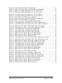
Figure 1. Study Area for Flathead River Instream Flow Study. .....................................................2
Figure 2. Flow chart of data analysis for Flathead River hydraulics and aquatic habitat...............5
Figure 3. Example of grid network developed from topography data............................................9
Figure 4. Example of depth contours for Flathead River, Site 2 105 cms......................................9
Figure 5. Example of velocity contours Flathead River Site 2, 105 cms. ....................................10
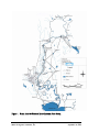
Figure 6. Spreadsheet template for habitat time series. ................................................................13
Figure 7. Example of Vlookup function for time series analysis. ................................................14
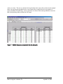
Figure 8. Habitat time series example for the site and reach........................................................15
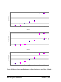
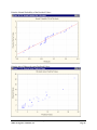
Figure 9. Observed versus predicted water surface elevations for three flows at Reach 1. .........17
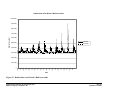
Figure 10. Histogram of observed and predicted water velocities for 246.55 cms at Reach 1. ...18
Figure 11. Water surface elevations at a range of discharges for Site 1, Flathead River. ............18
Figure 12. Hydrology time series Reaches 1 and 2. .....................................................................19
Figure 13. Hydrology time series Reach 3. ..................................................................................20
Figure 14. Average Discharge Reaches 1 and 2. ..........................................................................21
Figure 15. Average discharge Reach 3. ........................................................................................22
Flathead Instream Flow Investigation Project
Miller Ecological Consultants, Inc.
Page i
September 29, 2003
Figure 16.
Figure 17.
Figure 18.
Figure 19.
Figure 20.
Figure 21.
Figure 22.
Figure 23.
Figure 24.
Figure 25.
Figure 26.
Figure 27.
Figure 28.
Figure 29.
Figure 30.
Figure 31.
Figure 32.
Figure 33.
Figure 34.
Figure 35.
Figure 36.
Figure 37.
Figure 38.
Figure 39.
Figure 40.
Figure 41.
Figure 42.
Figure 43.
Figure 44.
Figure 45.
Figure 46.
Figure 47.
Figure 48.
Figure 49.
Figure 50.
Figure 51.
Figure 52.
Figure 53.
Reach 1 Bull trout habitat versus discharge. ...............................................................24
Reach 1 West slope cutthroat trout habitat versus discharge. .....................................24
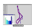
Bull trout sub-adult night habitat area, 105 cms, Reach 2. .........................................25
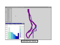
Bull trout sub-adult night habitat area, 169 cms, Reach 2. .........................................26
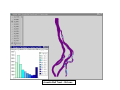
West slope cutthroat trout habitat area, 105 cms, Reach 2..........................................27
West slope cutthroat trout habitat area, 169 cms, Reach 2..........................................28
Reach 2 Bull Trout Habitat versus discharge..............................................................29
Reach 2 Westslope cutthroat trout habitat versus discharge. ......................................29
Reach 3 Bull trout habitat versus discharge. ...............................................................30
Reach 3 West slope cutthroat habitat versus discharge...............................................30
Annual habitat time series Reach 1 West slope cutthroat summer. ............................32
Annual habitat time series Reach 1 West slope cutthroat trout winter. ......................33
Habitat time series Reach 1 West slope cutthroat trout summer.................................34
Habitat time series Reach 1 West slope cutthroat trout winter. ..................................35
Annual habitat time series bull trout subadult night. ..................................................36
Annual habitat time series Bullt rout subadult day. ....................................................37
Annual habitat time series Reach 1 Bull trout adult....................................................38
Habitat time series Reach 1 Bull trout subadult night.................................................39
Habitat time series Reach 1 Bull trout subadult night.................................................40
Habitat time series Reach 1 Bull trout adult................................................................41
Annual habitat time series Reach 2 West Slope cutthroat trout summer. ...................42
Annual habitat time series Reach 2 West Slope cutthroat trout winter.......................43
Habitat time series Reach 2 West Slope cutthroat trout summer. ...............................44
Habitat time series Reach 2 West Slope cutthroat trout winter...................................45
Annual habitat time series Reach 2 Bull trout subadult night.....................................46
Annual habitat time series Reach 2 Bull trout subadult day. ......................................47
Annual habitat time series Reach 2 Bull trout adult....................................................48
Habitat time series Reach 2 Bull trout subadult night.................................................49
Habitat time series Reach 2 Bull trout subadult day. ..................................................50
Habitat time series Reach 2 Bull trout adult................................................................51
Annual habitat time series West Slope cutthroat trout. ...............................................52
Habitat time series Reach 3 West Slope cutthroat trout..............................................53
Annual habitat time series Reach 3 Bull trout subadult night.....................................54
Annual habitat time series Reach 3 Bull trout subadult day. ......................................55
Annual habitat time series Reach 3 Bull trout adult....................................................56
Habitat time series Reach 3 Bull trout subadult night.................................................57
Habitat time series Reach 3 Bull trout subadult day. ..................................................58
Habitat time series Reach 3 Bull trout adult................................................................59
Flathead Instream Flow Investigation Project
Miller Ecological Consultants, Inc.
Page ii
September 29, 2003
INTRODUCTION
Bonneville Power Administration (BPA) requested studies on the Flathead River from the South
Fork Flathead River downstream to Flathead Lake to determine changes in habitat availability
for fish in the Flathead River as a function of changes in river flow. The goal of this study was
to provide the physical framework for assessing changes in physical habitat in the river as a
function of flow for the species of interest and provide the tool for decision makers to assess
tradeoffs in river management scenarios.
The basis for this GIS approach comes from the Instream Flow Incremental Methodology and is
patterned after Bovee (1982), Bovee et al. (1998). We used the components of physical
hydraulic simulations, habitat suitability data, and the GIS analysis tool to develop habitat versus
discharge functions for the Flathead River. Components needed for this methodology include
habitat use information for the species of interest, physical geometry and hydraulics information
of geo-referenced physical data collected at each study site. Data included bed topography,
bathymetry, depth, velocity, substrate cover, and water surface elevations. These data provide
the physical framework for habitat analysis.
These physical data are then placed into a two-dimensional hydraulic simulation where the field
data is used to construct the model data sets. Models are calibrated for measured flows and
hydraulics simulated for the flows of interest. All output is geo-referenced for each study site
and the hydraulic simulations for each study site are passed to the habitat component.
Study Area
The study area includes the Flathead River from the South Fork confluence downstream to the
river mouth on Flathead Lake, Montana. The river was divided into three reaches. The first
reach begins at the South Fork confluence and extends downstream 17.6 km in mostly
homogeneous habitat with some island complexes. The second reach was the braided reach and
depositional area from the end of Segment 1 downstream to the end of the braided section. The
third reach extends from the lower end of the braided section to the mouth of Flathead Lake and
is characterized by low gradient and seasonal backwater effects from the lake impounded by
Kerr Dam (Figure 1). A study site was selected in each reach to represent the physical
characteristics of the reach. Each study site was more than 3 km in length (Table 1).
Table 1. Flathead River IFIM study Reach lengths and site lengths.
Reach
1
2
3
Total Length (km)
17.6
19.2
31.6
Flathead Instream Flow Investigation Project
Miller Ecological Consultants, Inc.
Site Length (km)
3.4
3.9
3.7
Page 1
September 29, 2003
Figure 1. Study Area for Flathead River Instream Flow Study.
Flathead Instream Flow Investigation Project
Miller Ecological Consultants, Inc.
Page 2
September 29, 2003
Objectives
There are three objectives for this study:
1. Develop comprehensive, spatial and tabular attribute database (IFIM models) to characterize
physical processes in the Flathead River affected by flow from Hungry Horse Dam.
2. Use IFIM models to compare the results of alternative dam operation strategies on aquatic
resources. Within each of three reaches, calibrate IFIM submodels to describe hydraulic
conditions under various flow volumes. Simulate changes in physical habitat conditions at
flows of interest.
3. Document results in reports, maps, and calibrated models in user manuals.
Flathead Instream Flow Investigation Project
Miller Ecological Consultants, Inc.
Page 3
September 29, 2003
METHODS
This project used a modified application of IFIM in three reaches of the Flathead River. The
entire river segment downstream of Hungry Horse Dam was mapped using GIS technology and
onstream ground truthing. Microhabitat use by fish life stages was provided by another BPA
project (9401000) and overlaid on the framework provided by this project. Target species
include bull trout (Salvelinus confluentus)and west slope cutthroat trout (Oncorhynchus clarki
lewisi). To accomplish these goals, MEC used a combination of hydraulic simulation and GIS
mapping on the Flathead River from the South Fork confluence to the mouth of Flathead Lake as
the base map for the overall analysis. The technical approach is presented in the following
sections.
General Approach
The approach for assessing instream flow needs for fish utilized hydraulic analysis and habitat
modeling in a modified incremental method to evaluate changes in quantity, quality, and
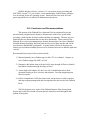
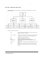
distribution of habitat with changes in flow (Figure 2). By collecting the hydraulic data in a
manner suitable to two-dimensional modeling of habitat, spatial distribution of habitat was
displayed with a Geographic Information System (GIS), and tabulations of habitat quantity and
quality were related to flow levels in the river.
Hydraulic modeling begins with construction of a digital terrain map for the study area. A
survey-grade Global Positioning System (GPS) was used to field map each study site, and data
points were used to construct a detailed topography map (or grid) of the channel. Multiple data
sets of water-surface elevations and point velocity measurements were used to calibrate a twodimensional hydraulic model to simulate depth and direction of flow through each site (Table 2).
The grid of resulting flow depths and velocities is then compared to habitat preference criteria for
species of interest to determine location and quality of resulting habitat.
Table 2. Hydraulic measurements recorded on the Flathead River above Flathead Lake,
Montana.
Date
Discharge (m3/s)
Reaches 1-2 Reach 3
Measurement
Bed topography, water surface elevations,
velocity profiles, substrate mapping
20 June 2000
594.65
624.88 Water surface elevations
3-7 January 2001
105.17
108.15 Water surface elevations
Note: Reported discharge for Reaches 1 and 2 are from USGS gaging station 12363000
(Flathead River at Columbia Falls, MT). Discharge for Reach 3 is the combined flow reported
from USGS gaging stations 12363000, 12366000 (Whitefish River near Kalispell, MT), and
12365000 (Stillwater River near Whitefish, MT).
2-9 August 1999
246.56
257.10
Flathead Instream Flow Investigation Project
Miller Ecological Consultants, Inc.
Page 4
September 29, 2003
Field Data
Channel
Topography
Water Surface
Elevations
Velocity
Profile
Hydraulic
Modeling
Output: depth and velocity
pairings for individual nodes.
Habitat Suitability
Analysis
from previous slide
Fish Data
(Depth/Velocity)
GIS
Framework
Output: Quantified
representation of suitable
habitat for a range of
measured flows.
Output: Regression equation
for suitability data
Time Series
Analysis
GIS
Framework
Output: Quantified habitat suitability
for non-measured flows and flows
significant to the determination of
future management of the system.
Hydrology
Figure 2. Flow chart of data analysis for Flathead River hydraulics and aquatic habitat.
Flathead Instream Flow Investigation Project
Miller Ecological Consultants, Inc.
Page 5
September 29, 2003
Habitat modeling thus requires information on fish utilization of certain depths and velocities of
flow, in addition to utilization of certain substrate, cover, and other channel conditions. The
habitat suitability functions are then used as a filter against the grid of depth and velocity values
predicted by the hydraulic model to estimate suitability of habitat in each grid cell at the site.
The area of grid cells with suitable habitat are then summed to obtain total usable area for a
given streamflow level. BPA requested that a geographic information system (GIS) be
developed to provide these functions for the project.
Hydraulic data was measured in a manner compatible with both standard and modified IFIM
techniques. River gradient and flow was measured using standard surveying techniques.
Channel morphology was measured using a boat mounted GPS hydroacoustic system to develop
detailed river topography maps and digital terrain maps that could be incorporated in GIS. These
maps were developed for two mile subreaches of each of the three main reaches. A total of six
miles of digital terrain mapping was conducted on the river. The digital terrain maps were
linked to above water surveys to the high water mark at each of the two mile reaches to establish
ground topography for higher flow regimes for the modeling effort. Substrate and cover data
was collected using visual or tactile methods to determine sediment at cross-sections established
for the IFIM modeling. Habitat suitability was developed concurrently in BPA Project 9401000.
The data from that project (Muhlfeld 2002) was used as input to the habitat model for the IFIM
analysis.
River hydrology for determining flow scenarios and flow operations was calculated using
existing hydrology from USGS records for the Flathead River and Hungry Horse Dam. A flow
time series was constructed using approximately ten years of daily flow data and incorporating
that into a spreadsheet for flow comparison alternatives. Flow comparisons were made for both
flow scenarios. The specific methods for the project are listed below.
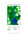
River Channel Change Analysis and Land Use/Land Cover Mapping
The main objectives of this portion of the project were: 1) Identify areas of the Flathead River
channel that are dynamically changing and, 2) Map land use and land cover along the river. A
detailed description of the land use/land cover mapping is provided in Appendix A.
This task involved processing the river channel and land use/land cover data to produce
deliverable products. The old and new river channel GIS layers were overlain to produce a layer
that identifies all of the areas where the river course has shifted between the two time periods.
This simple change layer highlights the most dynamic reaches of the river. A second analysis
utilized historical resource photography to determine what land use/land cover was present
before changes occurred at a given site. This analysis produced a complex (“from and to”)
change map. From this information, BPA can determine which land uses are most likely to be
affected by river dynamics.
Flathead Instream Flow Investigation Project
Miller Ecological Consultants, Inc.
Page 6
September 29, 2003
Topographic Mapping
Each study site was surveyed with a survey-grade GPS for the purpose of constructing a digital
terrain model for the site. The GPS provided latitude, longitude, and elevation of each point to an
accuracy of about 0.1 foot for both horizontal and vertical resolution. Horizontal stations and
elevations were georeferenced to known points of origin in the vicinity of each study site. A
sufficient number of points were surveyed on the ground to enable construction of a digital terrain
model for the study reach. In the vicinity of the channel, points were spaced to define channel
geometry both in plan form and cross section. Channel geometry points were collected up to the
typical high-water marks to establish ground topography for modeling high flow regimes.
Substrate and cover were recorded for each site, along with field notes describing general stream
and habitat conditions at the study site and reference photos for the area.
Hydraulic Data Collection
Two-dimensional hydraulic modeling requires channel geometry data, multiple water-surface
elevation data sets, and multiple velocity data sets. Thus, the specific hydraulic data collected at
each site includes stream bed elevations, mean column velocity at selected locations (multiple
collections at each habitat type), visual estimates of dominant and subdominant substrate size and
percent embeddedness, and percent cover. All hydraulic data were georeferenced for inclusion in
the digital terrain model of the site and the associated GIS data base. The following procedures
were used to obtain the necessary data.
Stream Bed Elevations The survey-grade GPS was used to collect stream bed elevations
as described above. Above-water points also were surveyed using standard techniques
and georeferenced for linkage to GIS.
Water Velocities At a selected number of locations within each study site, water velocity
was measured for use in hydraulic model calibration. Multiple measurements were taken
in each specific site for use in model calibration.
Substrate Composition Substrate composition was visually estimated at each site for all
habitats. Substrate was denoted for the following categories:
·
·
·
·
·
·
·
·
Aquatic vegetation
Silt
Sand
Small gravel (0.25 - 1.0 inch)
Large Gravel (>1.0 - 3.0 inch)
Cobble (>3.0 - 10.0 inch)
Boulder (>10.0 inch)
Bedrock
The substrate was categorized by dominant and subdominant size class. The substrate
classification system was modified to provide the information required for the habitat
Flathead Instream Flow Investigation Project
Miller Ecological Consultants, Inc.
Page 7
September 29, 2003
suitability criteria. This method of substrate categorization can be adapted to most of the
usual substrate codes in the existing habitat suitability criteria.
Cover was visually estimated by percentage. The following cover types were used:
Velocity Refuge: any instream object that provides a velocity refuge for the
species of interest. This could include objects such as boulders, root wads, large woody
debris or other such objects.
Visual Isolation: any object that provides visual isolation for the species of interest
such as overhanging vegetation, undercut banks, or other such items.
Combination Cover: any cover that provides both velocity refuge and visual
isolation. This could be any combination of the cover items listed above or a single cover
object such as a downfall that provides both velocity refuge and visual isolation.
No Cover: absence of cover will also be noted.
The full set of data was recorded at one flow (Table 2). Repeat measurements of water-surface
elevations were taken at low and high flows. During these measurements water-surface
elevations were surveyed at each study site. These stage-discharge measurements provided the
data necessary for model calibration and for extending the range of hydraulic simulations.
Two-Dimensional Hydraulic Modeling
Two-dimensional hydraulic modeling was accomplished in the Surface-water Modeling System
(SMS) using the Corps of Engineers RMA2 model. This model was developed specifically to
look at two-dimensional velocity vectors in river systems, and is capable of handling element (i.e.,
grid cell) wetting and drying as flows are increased or decreased. This model operates on a grid
developed from the digital terrain model for each study site, and output can be linked to GIS
models for analysis and display of habitat availability (Appendix B).
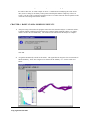
The 2-D model uses the georeferenced field data collected from each study site. Data inputs
include maps of site topography, substrate, and flow impediments; a stage-discharge relationship
at the downstream end of the site; and calibration and validation data throughout the reach.
Model calibration and validation data consist of depth and velocity measurements taken at know
flow rates and locations in the study site, usually at points upstream of impediments, along one or
more cross sections, and scattered throughout the reach. The GPS survey data is used to develop
a grid system to represent the stream geometry (Figure 3). This mesh is combined with the
hydraulic data to simulate water depths and velocities for a range of flow conditions (Figures 4
and 5).
Flathead Instream Flow Investigation Project
Miller Ecological Consultants, Inc.
Page 8
September 29, 2003
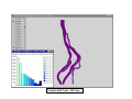
Figure 3. Example of grid network developed from topography data.
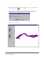
Figure 4. Example of depth contours for Flathead River, Site 2 105 cms.
Flathead Instream Flow Investigation Project
Miller Ecological Consultants, Inc.
Page 9
September 29, 2003
Figure 5. Example of velocity contours Flathead River Site 2, 105 cms.
Habitat Suitability Curves
Species habitat-suitability criteria are required for the habitat analysis. The recommended
approach is to develop site-specific criteria for each species and life stage of interest. Habitat
suitability criteria that accurately reflect the habitat requirements of the species of interest are
essential to conducting meaningful and defensible instream flow analyses. The curves used in this
study will fit that criterion. Site specific curves were developed for the study by Muhlfeld (2002).
Calculation of habitat suitability criteria for a two-dimensional hydraulic model requires use of a
bivariate analysis of depth-velocity paired data to calculate fish preference for depth and velocity
in the stream reach.
An analysis approach was developed by Miller Ecological (2001, Appendix C) for this suitability
criteria. A bivariate statistical analysis was used to develop habitat suitability criteria for each
species with sufficient data. This analysis first plotted bivariate histograms, then converted those
Flathead Instream Flow Investigation Project
Miller Ecological Consultants, Inc.
Page 10
September 29, 2003
to a 3-dimensional surface and finally computed a polynomial expression to compute suitability
values that replicate the 3-D surface.
GIS Model
The basis for this GIS approach comes from the Instream Flow Incremental Methodology and is
patterned after Bovee (1982), Bovee et al. (1998). We used the components of physical
hydraulic simulations, habitat suitability data, and the GIS analysis tool to develop habitat use
information. The original concept for this approach was presented in Miller Ecological
Consultants, Inc. and SAIC (2000). The current application of the GIS approach included a time
series analysis of habitat based on flow scenarios in the Flathead.
Components needed for this methodology include habitat use information for the species of
interest, physical geometry and hydraulics information of geo-referenced physical data collected
at each study site. Data included bed topography, bathymetry, depth, velocity, substrate cover,
and water surface elevations. These data provide the physical framework for habitat analysis.
These physical data are then placed into a two-dimensional hydraulic simulation where the field
data is used to construct the model data sets. Models are calibrated for measured flows and
hydraulics simulated for the flows of interest. All output is geo-referenced for each study site
and the hydraulic simulations for each study site are passed to the habitat component.
GIS Based Weighted Usable Area Model
After pre processing data for habitat suitability and hydraulic simulations, these components are
used for simulation of usable habitat. The geo-referenced hydraulic data sets are imported into
Arcview and combined with habitat suitability data for the analysis. The habitat suitability
equations are combined with the geo-referenced output from the hydraulic data sets and habitat
suitabilities are calculated based on the depth and velocity at each point within the site. Habitat
maps are created and tabular data sets produced that are used in the habitat time series. A
detailed description of the analytical steps is provided in the software manual (Appendix B).
The combination of hydraulics and habitat are repeated at each study site for all flows of interest
and for all species and life stages. The habitat areas for each flow for each species are extracted
from the GIS output and either copied or typed into the time series spreadsheet to conduct the
habitat time series.
Habitat versus Discharge Modeling
Habitat suitability modeling for each species of interest is accomplished in an Arcview GIS
analysis (Appendix B). The Arcview instream habitat model relies on inputs from both the 2-D
hydraulic modeling and the habitat suitability criteria described above. These inputs are
Flathead Instream Flow Investigation Project
Miller Ecological Consultants, Inc.
Page 11
September 29, 2003
provided in the form of data layers within the GIS and parameters for spatial queries. Data
layers corresponding to flow depths and velocities are provided by the 2-D hydraulic modeling.
Specific habitat criteria developed from the suitability analyses described above are then used to
conduct GIS queries. In this way, the amount of area within the study site that matches a
particular species’ habitat use can be determined for a specified flow rate. Multiple layers of
usable habitat were generated, corresponding to each species, life stage, and flow of interest.
The analysis can be output as a 2D map and linked to a GIS base map or plotted as hard copy for
visual presentation of the results. Summation of total habitat for each species and simulated flow
results in a habitat-flow relationship by species that becomes input for the habitat-time series
analysis.
Habitat Time Series
The actual habitat experienced by the fish in any river depends on the flow regime of the river.
The development of habitat conditions over a period of time is an integral part of the comparison
of flow regimes. Habitat time series is the decision point in IFIM (Bovee 1982). Habitat time
series analysis requires the following data: total usable habitat for each species and life stage at
each flow of interest, preferably over a range from normal high to low flow; hydrology data for
current conditions, usually weekly or daily flow for a range of water years; and hydrology for the
proposed operation for the same dates as the current conditions.
MEC conducted time series evaluations on several different flow regimes. For each flow regime
assessed, we conducted both hydrology and habitat time series analysis to calculate both flowand habitat statistics. These values allowed a direct comparison of the changes that occur in both
flow and habitat under a range of conditions. These tabular data can be displayed for each flow
scenario to represent the spatial habitat distributions.
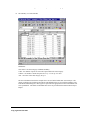
Habitat time series uses a spreadsheet format with data arranged in columns and rows that
combines the hydrology over time with the habitat use as a function of discharge. These values
are converted to area of habitat for the study site and then area of habitat for the reach.
Comparisons of change in habitat over time for each flow of interest are possible with this
spreadsheet setup. The steps to use the spreadsheet for analysis are as follows:
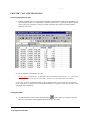
The habitat time series spreadsheet is arranged with data in column format. Cell A1 contains the
title. Cell A2 contains the name of the river. Cells A4 through A6 are titles for species and life
stage. The species names and life stages are typed into Cells B4, B5, and B6 (Figure 6).
The hydrology data is placed in columns A, B and C. Rows 10 through 12 of those columns
contain header information. Column A contains the Date, and Columns B and C contain the
hydrology data. Column B contains the baseline hydrology titled “Pre-dam”. Column C
contains the hydrology for the “Post-dam” alternative.
To the right of the hydrology columns are a look-up table with regression coefficients and
functions for the weighted usable area for juvenile and adults of the species. The headers denote
discharge (Q), habitat, and the A and B terms for the functions. The cells contain the formulas
Flathead Instream Flow Investigation Project
Miller Ecological Consultants, Inc.
Page 12
September 29, 2003
that calculate the A and B terms. The discharge and habitat values are generated in the GIS Base
habitat model and copied or typed into the cells. The data for the blocks should start in cells of
the time series spreadsheet contained in the distribution CD. The habitat for the site for each
flow is analyzed by date and flow regime. The rows must be identical for the correct analysis.
The habitat calculations are based on a Vlookup formula contained in cells R12, S12 and higher
(Figure 7).
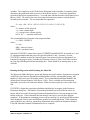
Figure 6. Spreadsheet template for habitat time series.
Flathead Instream Flow Investigation Project
Miller Ecological Consultants, Inc.
Page 13
September 29, 2003
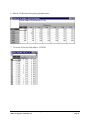
Figure 7. Example of Vlookup function for time series analysis.
Calculation of habitat for the site is completed for each life stage. The spreadsheet is set up to
calculate habitat for each species and life stage of interest. The analysis requires that the formula
be copied into the appropriate number of rows that correspond to every row containing
hydrology in Columns B and C.
There are corresponding formulas in columns R, S, T and U to calculate the total habitat for the
reach. The amount of habitat for the site is multiplied by the reach distance to compute total
habitat for the reach (Figure 8). Again, the number of rows corresponds to the number of
hydrology data points.
This spreadsheet can also be used to graphically display the data to compare habitat over time.
This identifies the information visually to give the capability of displaying where changes occur
in habitat over time with the proposed flow regimes. Those results are presented in the next
section.
The GIS based model calculated habitat from geo referenced hydraulic data and habitat
suitability indices. The resulting values calculate habitat time series using the included
spreadsheet. The habitat time series relies on formulas in specific cells to calculate habitat
Flathead Instream Flow Investigation Project
Miller Ecological Consultants, Inc.
Page 14
September 29, 2003
values over time. The user is cautioned to keep the data in the same cells as those in the example
sheet. An experienced spreadsheet user can customize the example sheet for any number of
species and dates for hydrology. In our experience it is best to limit each spreadsheet to no more
than four hydrology data sets and four life stages.
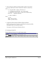
Figure 8. Habitat time series example for the site and reach.
Flathead Instream Flow Investigation Project
Miller Ecological Consultants, Inc.
Page 15
September 29, 2003
RESULTS
The results presented here provide the details of the instream flow analysis for the Flathead
River reaches 1, 2 and 3. A more comprehensive data set is included in the distribution compact
disk (CD) with the Arcview projects files that contain all simulations for all species and life
stages at each site. Those data present the visual results of the analysis as well as provide grid
files for additional analysis in GIS as needed by BPA and Montana Fish, Wildlife and Parks.
Model Calibration
The hydraulic models were calibrated to both water surface and water velocity to insure an
accurate representation of the measured flows for each study site. Water surface elevations,
from the simulations, accurately represent measured flows for low, mid and high flow ranges
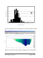
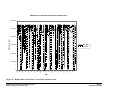
(Figure 9). Water velocities were measured at mid-flow for all three study sites. A comparison
of measured water velocity to predicted shows that the predicted velocities, in general, match
measured water velocities with a slight underprediction (Figure 10).
Habitat suitability data were applied for west slope cutthroat trout for reach 1 and 2, summer and
winter curves, and west slope cutthroat trout year round for reach 3 (Muhlfeld 2002). In
addition, bull trout sub-adult criteria for day and bull trout sub-adult criteria for night were
applied to sites 1, 2 and 3. Bull trout adult data were applied to reaches 1, 2 and 3. The only diel
comparison was made for sub-adult bull trout in reaches 1 and 2.
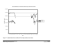
Model hydraulics show that both depths and velocities vary as expected for each of the sites and
reaches (See distribution CD). There is a significant difference between the wetted channel
width for the 105 cms and the 169 cms values in riffle areas. Fluctuations in riffles between
these two flows can reach approximately 40 meters (Figure 11).
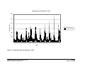
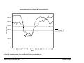
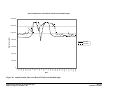
Hydrology time series was generated for pre-dam and post-dam conditions to compare the
unregulated and regulated system. The main differences in the hydrology are shown in the
winter baseflow period where post-dam flows are highly variable and in the reduction of peak
flows during certain conditions, especially during peak snowmelt runoffs. Historically, pre-dam
conditions had summer peak flows during snowmelt of over 2,000 cms and very stable but lower
baseflows. Current post-dam conditions show that the baseflow period can vary by as much
200cms or more and that peak flows are generally less than 1,500 cms (Figure 12). There is a
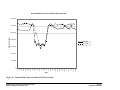
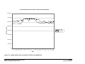
similar representation of high hydrology for reach 3. The difference between hydrology in reach
3 and reaches 1 and 2 is the additional inflow from the White Fish and Stillwater rivers that enter
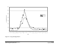
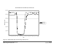
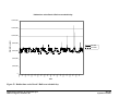
the Flathead at the upstream end of reach 3 (Figure 13). Average annual hydrology were
developed from the 1940-49 pre-dam data and the 1993-2002 post-dam hydrology. These
annual hydrographs allow the comparison of baseflow and peak flow conditions to show the
differences between those two seasonal characateristics (Figures 14 and 15). The baseflow
period is much more variable in the post-dam hydrology and peak flows truncated when
compared with the pre-dam hydrology showing very stable baseflows and higher peak flows.
Flathead Instream Flow Investigation Project
Miller Ecological Consultants, Inc.
Page 16
September 29, 2003
3
105.17 m /s
919.5
919
Water Surface Elevation
918.5
918
917.5
917
916.5
916
915.5
915
3
246.55 m /s
920
919.5
Water Surface Elevation (m)
919
918.5
Predicted
918
Observed
917.5
917
916.5
916
915.5
3
594.65 m /s
921
920.5
Water Surface Elevation (m)
920
919.5
919
918.5
918
917.5
917
916.5
916
0
1
2
3
4
5
6
7
8
Continuity Line
Figure 9. Observed versus predicted water surface elevations for three flows at Reach 1.
Flathead Instream Flow Investigation Project
Miller Ecological Consultants, Inc.
Page 17
September 29, 2003
50
45
40
Number of Observations
35
Predicted
30
Observed
25
20
15
10
5
0
00.
2
0.
20.
4
0.
40.
6
0.
60.
8
0.
81.
0
1.
01.
2
1.
21.
4
1.
41.
6
1.
61.
8
1.
82.
0
2.
02.
2
2.
22.
4
2.
42.
6
2.
62.
8
2.
83.
0
3.
03.
2
3.
23.
4
3.
43.
6
3.
63.
8
3.
84.
0
0
Mean Column Velocity (m/s)
Figure 10. Histogram of observed and predicted water velocities for 246.55 cms at Reach
1.
Figure 11. Water surface elevations at a range of discharges for Site 1, Flathead River.
Flathead Instream Flow Investigation Project
Miller Ecological Consultants, Inc.
Page 18
September 29, 2003
Hydrology time series Reaches 1 and 2
3000.0
2500.0
Discharge (m3/s)
2000.0
Pre-dam 1940-49
1500.0
Post-dam 1993-2002
1000.0
500.0
0.0
1
6/
1
2/
/1
10
1
6/
1
2/
/1
10
1
6/
1
2/
/1
10
1
6/
1
2/
/1
10
1
6/
1
2/
/1
10
1
6/
1
2/
/1
10
1
6/
1
2/
/1
10
1
6/
1
2/
/1
10
1
6/
1
2/
/1
10
1
6/
1
2/
/1
10
Date
Figure 12. Hydrology time series Reaches 1 and 2.
Flathead Instream Flow Investigation Project
Miller Ecological Consultants, Inc.
Page 19
September 29, 2003
Hydrology Time series Reach 3
3000.0
2500.0
Discharge (m3/s)
2000.0
Pre-dam discharge (1940-49)
1500.0
Post-dam discharge (1993-2002)
1000.0
500.0
0.0
1
6/
1
2/
/1
10
1
6/
1
2/
/1
10
1
6/
1
2/
/1
10
1
6/
1
2/
/1
10
1
6/
1
2/
/1
10
1
6/
1
2/
/1
10
1
6/
1
2/
/1
10
1
6/
1
2/
/1
10
1
6/
1
2/
/1
10
1
6/
1
2/
/1
10
Date
Figure 13. Hydrology time series Reach 3.
Flathead Instream Flow Investigation Project
Miller Ecological Consultants, Inc.
Page 20
September 29, 2003
1400.0
1200.0
Discharge (m3/s)
1000.0
800.0
Post Dam
Pre Dam
600.0
400.0
200.0
4/
9
4/
23
5/
7
5/
21
6/
4
6/
18
7/
2
7/
16
7/
30
8/
13
8/
27
9/
10
9/
24
10
/
10 8
/2
2
11
/5
11
/1
9
12
/
12 3
/1
12 7
/3
1
1/
1
1/
15
1/
29
2/
12
2/
26
3/
12
3/
26
0.0
Date
Figure 14. Average Discharge Reaches 1 and 2.
Flathead Instream Flow Investigation Project
Miller Ecological Consultants, Inc.
Page 21
September 29, 2003
1400
1200
1000
Average Discharge (m3/s)
Pre-Dam
Post Dam
800
600
400
200
31-Dec
17-Dec
3-Dec
19-Nov
5-Nov
22-Oct
8-Oct
24-Sep
10-Sep
27-Aug
13-Aug
30-Jul
16-Jul
2-Jul
18-Jun
4-Jun
21-May
7-May
23-Apr
9-Apr
26-Mar
12-Mar
26-Feb
12-Feb
29-Jan
15-Jan
1-Jan
0
Date
Figure 15. Average discharge Reach 3.
Flathead Instream Flow Investigation Project
Miller Ecological Consultants, Inc.
Page 22
September 29, 2003
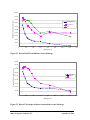
Habitat Simulations
Habitat for all three reaches was simulated using the combination of two-dimensional hydraulic
model and GIS weighted useable area model to generate weighted useable area in m2 per
kilometer for each of the three reaches. Species with several life stages have similar patterns of
weighted useable area discharge functions in reach 1. Bull trout habitat versus discharge shows
a similar relationship with the highest weighted useable area occurring at the lower flows and
value of weighted useable area being reduced at higher flows for both day and night usage and
for adults (Figure 16). West slope cutthroat trout for fall and winter criteria and summer show a
similar relationship with the highest weighted useable area at the lower flow conditions (Figure
17). Both of these species show that the useable habitat area is more widely distributed through
the channel at the lower flow conditions than they are at the high flow conditions. This is likely
a result of the increased velocities that occur as flows increase with most of the habitat occurring
along the lower velocity margins of the river and around the islands rather than in the main
channel (Figures 18 through 21).
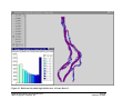
The reduction in suitable near shore habitat is particularly important for bull trout subadults.
Muhlfeld (2003) reports a distinct difference in diel habitat use by subadult bull trout. The
shallow habitat near the river shorelines is used at night by subadult bull trout. The quality of
this habitat is higher when the river is stable for longer periods (several weeks) and benthic
productivity can increase.
Habitat areas for both bull trout and west slope cutthroat trout for reach 2 shows similar response
of weighted useable area to discharge with the higher values at the lower discharges. There is a
difference between reach 1 and reach 2 in the response shape of the curves showing that there is
a difference between those two reaches for hydraulic conditions. The curve that is most different
in reach 2 from those in reach 1 is sub-adult night bull trout (Figure 22) and the fall and winter
west slope cutthroat trout curves (Figure 23).
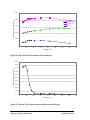
Reach 3 is hydraulically controlled by the water surface elevation of Flathead Lake and therefore
there is very little change with discharge to the amount or the shape of the weighted useable area
criteria curve for bull trout. In general, it appears to be a scaling factor of where that habitat is
located based on depth of the water and current velocity. In general, there is very little
difference between the amount of habitat for each life stage at high or low flow as those response
curves are very flat. There is a difference in absolute value for weighted useable area between
the different life stages of sub-adult night, sub-adult day and adult bull trout (Figure 24).
West slope cutthroat trout, in contrast, has a distinct relationship between discharge and
weighted useable area in reach 3 (Figure 25). As with the upper two reaches, the habitat is
greatest at the lower flow range and then declines in the upper flow ranges. There is a
substantial decline in reach 3 response which may be due to depth differences as well as velocity
differences.
Flathead Instream Flow Investigation Project
Miller Ecological Consultants, Inc.
Page 23
September 29, 2003
90,000
70,000
Subadult (night)
Subadult (day)
60,000
2
Weighted Usable Area (m per km)
80,000
Adult
50,000
40,000
30,000
20,000
10,000
0
0
100
200
300
400
500
600
700
800
900
3
Discharge (m /s)
Figure 16. Reach 1 Bull trout habitat versus discharge.
80,000
2
Weighted Usable Area (m per km)
70,000
60,000
50,000
Fall/winter
Summer
40,000
30,000
20,000
10,000
0
0
100
200
300
400
500
600
700
800
3
Discharge (m /s)
Figure 17. Reach 1 West slope cutthroat trout habitat versus discharge.
Flathead Instream Flow Investigation Project
Miller Ecological Consultants, Inc.
Page 24
September 29, 2003
900
Figure 18. Bull trout sub-adult night habitat area, 105 cms, Reach 2.
Flathead Instream Flow Investigation Project
Miller Ecological Consultants, Inc.
Page 25
September 29, 2003
Figure 19. Bull trout sub-adult night habitat area, 169 cms, Reach 2.
Flathead Instream Flow Investigation Project
Miller Ecological Consultants, Inc.
Page 26
September 29, 2003
Figure 20. West slope cutthroat trout habitat area, 105 cms, Reach 2.
Flathead Instream Flow Investigation Project
Miller Ecological Consultants, Inc.
Page 27
September 29, 2003
Figure 21. West slope cutthroat trout habitat area, 169 cms, Reach 2.
Flathead Instream Flow Investigation Project
Miller Ecological Consultants, Inc.
Page 28
September 29, 2003
200,000
180,000
Subadult (night)
140,000
Subadult (day)
2
Weighted Usable Area (m per km)
160,000
120,000
Adult
100,000
80,000
60,000
40,000
20,000
0
0
200
400
600
800
1000
1200
1400
1600
3
Discharge (m /s)
Figure 22. Reach 2 Bull Trout Habitat versus discharge.
180,000
140,000
120,000
2
Weighted Usable Area (m per km)
160,000
Fall/winter
100,000
Summer
80,000
60,000
40,000
20,000
0
0
200
400
600
800
1000
1200
1400
3
Discharge (m /s)
Figure 23. Reach 2 Westslope cutthroat trout habitat versus discharge.
Flathead Instream Flow Investigation Project
Miller Ecological Consultants, Inc.
Page 29
September 29, 2003
1600
250,000
Subadult (night)
Subadult (day)
2
Weighted Usable Area (m per km)
200,000
Adult
150,000
100,000
50,000
0
0
200
400
600
800
1000
1200
1400
1600
1000
1200
1400
1600
3
Discharge (m /s)
Figure 24. Reach 3 Bull trout habitat versus discharge.
200,000
180,000
140,000
2
Weighted Usable Area (m per km)
160,000
120,000
100,000
80,000
60,000
40,000
20,000
0
0
200
400
600
800
3
Discharge (m /s)
Figure 25. Reach 3 West slope cutthroat habitat versus discharge.
Flathead Instream Flow Investigation Project
Miller Ecological Consultants, Inc.
Page 30
September 29, 2003
Habitat Time Series
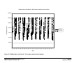
Habitat time series analysis used ten-year and annual hydrology. The hydrology for west slope
cutthroat trout was divided into summer and winter seasons. The response of habitat to flow is
similar to the flow regime change between the pre-dam and post-dam conditions. Pre-dam
conditions for summer shows that the habitat increased sharply after runoff and was stable in the
summer baseflow period. Post-dam conditions show that the response of habitat to flow is
slower and also is much more variable in the summer baseflow period (Figure 26). Winter
baseflows for west slope cutthroat trout show that the winter pre-dam period was very stable
with a relatively high amount of habitat area and that current conditions have much more
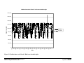
variable habitats over time (Figure 27). The ten-year time series also show that the variability
and magnitude of habitat response continues over time from what was calculated in the annual
hydrograph series (Figures 28 and 29). The baseflow period is much more variable than during
the post-dam conditions, than the pre-dam conditions, and habitat values for pre-dam can be
higher at times than the post-dam period.
Bull trout sub-adults show a very similar response to flow for day and night. Although the
nighttime suitability criteria for bull trout sub-adults shows that the total amount of habitat in
pre-dam conditions was higher during the winter baseflows than currently exist. Also there is
more stability during the pre-dam conditions during summer and winter baseflows than exist for
both bull trout sub-adult nighttime and daytime criteria (Figures 30 and 31). Bull trout adult
habitat in reach 1 shows a similar stability during the pre-dam, baseflow conditions and much
more variability during the post-dam baseflow conditions (Figures 32 and 33).
Habitat characteristics for reach 2 are similar to those shown for reach 1 with west slope
cutthroat trout having more variability in baseflow conditions post-dam than pre-dam. The curve
habitat area during runoff in summer periods show that there is very little difference between the
reach 2 conditions pre- and post-dam. There is a distinct difference for winter west slope
cutthroat trout habitat showing both less habitat and more variability in the habitat on a daily
basis in the post-dam condition than was shown in the pre-dam condition (Figures 34 and 35).
The analysis of the ten-year time series again shows west slope cutthroat trout to be more
variable post-dam than pre-dam with more stability and higher habitat availability in the pre-dam
conditions (Figures 36 and 37). Bull trout sub-adults in reach 2 show the habitat in pre-dam
conditions for nighttime was more abundant and more stable during baseflows than the post-dam
period, which has more daily variability in habitat. This is shown both in the annual times series
in Figures 38 and 39, and also in the ten-year time series in Figures 41 through 43.
Reach 3 habitat conditions show that the post-dam conditions for west slope cutthroat trout have
better habitat than were shown in the pre-dam conditions (Figures 44 and 45). Bull trout habitat
for reach 3 shows that there is slightly more quanitity of habitat in the post-dam hydrology than
pre-dam hydrology for sub-adults and adults but there is more variability during baseflow
conditions of that habitat (Figures 46 through 53).
Flathead Instream Flow Investigation Project
Miller Ecological Consultants, Inc.
Page 31
September 29, 2003
Annual habitat time series Reach 1 West slope cutthroat summer
1,400,000
1,200,000
Habitat area (m2)
1,000,000
800,000
Pre Dam
Post Dam
600,000
400,000
200,000
1/
1
1/
15
1/
29
2/
12
2/
26
3/
12
3/
26
4/
9
4/
23
5/
7
5/
21
6/
4
6/
18
7/
2
7/
16
7/
30
8/
13
8/
27
9/
10
9/
24
10
/
10 8
/2
2
11
/5
11
/1
9
12
/
12 3
/1
12 7
/3
1
0
Date
Figure 26. Annual habitat time series Reach 1 West slope cutthroat summer.
Flathead Instream Flow Investigation Project
Miller Ecological Consultants, Inc.
Page 32
September 29, 2003
Annual habitat time series Reach 1 West slope cutthroat trout winter
1,200,000
1,000,000
Habitat Area (m2)
800,000
Pre Dam
600,000
Post Dam
400,000
200,000
12/31
12/17
12/3
11/19
11/5
10/22
10/8
9/24
9/10
8/27
8/13
7/30
7/16
7/2
6/18
6/4
5/7
5/21
4/23
4/9
3/26
3/12
2/26
2/12
1/29
1/15
1/1
0
Date
Figure 27. Annual habitat time series Reach 1 West slope cutthroat trout winter.
Flathead Instream Flow Investigation Project
Miller Ecological Consultants, Inc.
Page 33
September 29, 2003
Habitat time series Reach 1 West slope cutthroat trout summer
1,400,000
1,200,000
Habitat Area (m2)
1,000,000
800,000
Pre Dam
Post Dam
600,000
400,000
200,000
0
4/1
10/1
4/1
10/1
4/1
10/1
4/1
10/1
4/1
10/1
4/1
10/1
4/1
10/1
4/1
10/1
4/1
10/1
4/1
10/1
Date
Figure 28. Habitat time series Reach 1 West slope cutthroat trout summer.
Flathead Instream Flow Investigation Project
Miller Ecological Consultants, Inc.
Page 34
September 29, 2003
Habitat time series Reach 1 West slope cutthroat trout winter
1,200,000
1,000,000
Habitat Area (m2)
800,000
Pre Dam
600,000
Post Dam
400,000
200,000
0
4/1
10/1
4/1
10/1
4/1
10/1
4/1
10/1
4/1
10/1
4/1
10/1
4/1
10/1
4/1
10/1
4/1
10/1
4/1
10/1
Date
Figure 29. Habitat time series Reach 1 West slope cutthroat trout winter.
Flathead Instream Flow Investigation Project
Miller Ecological Consultants, Inc.
Page 35
September 29, 2003
Annual habitat time series bull trout subadult night
1,000,000
900,000
800,000
Habitat area (m2)
700,000
600,000
Pre Dam
500,000
Post Dam
400,000
300,000
200,000
100,000
12/31
12/17
12/3
11/19
11/5
10/22
10/8
9/24
9/10
8/27
8/13
7/30
7/16
7/2
6/18
6/4
5/7
5/21
4/23
4/9
3/26
3/12
2/26
2/12
1/29
1/15
1/1
0
Date
Figure 30. Annual habitat time series bull trout subadult night.
Flathead Instream Flow Investigation Project
Miller Ecological Consultants, Inc.
Page 36
September 29, 2003
Annual habitat time series Bull trout sub adult day
1,400,000
1,200,000
Habitat Area (m2)
1,000,000
800,000
Pre Dam
Post Dam
600,000
400,000
200,000
12/31
12/17
12/3
11/19
11/5
10/22
10/8
9/24
9/10
8/27
8/13
7/30
7/16
7/2
6/18
6/4
5/7
5/21
4/23
4/9
3/26
3/12
2/26
2/12
1/29
1/15
1/1
0
Date
Figure 31. Annual habitat time series Bullt rout subadult day.
Flathead Instream Flow Investigation Project
Miller Ecological Consultants, Inc.
Page 37
September 29, 2003
Annual habitat time series Reach 1 Bull trout adult
1,600,000
1,400,000
1,200,000
Habitat Area (m2)
1,000,000
Pre Dam
800,000
Post Dam
600,000
400,000
200,000
12/31
12/17
12/3
11/19
11/5
10/22
10/8
9/24
9/10
8/27
8/13
7/30
7/16
7/2
6/18
6/4
5/7
5/21
4/23
4/9
3/26
3/12
2/26
2/12
1/29
1/15
1/1
0
Date
Figure 32. Annual habitat time series Reach 1 Bull trout adult.
Flathead Instream Flow Investigation Project
Miller Ecological Consultants, Inc.
Page 38
September 29, 2003
Habitat time series Reach 1 Bull trout subadult night
1,000,000
900,000
800,000
Habitat area (m2)
700,000
600,000
Pre Dam
500,000
Post Dam
400,000
300,000
200,000
100,000
4/1
10/1
4/1
10/1
4/1
10/1
4/1
10/1
4/1
10/1
4/1
10/1
4/1
10/1
4/1
10/1
4/1
10/1
4/1
10/1
0
Date
Figure 33. Habitat time series Reach 1 Bull trout subadult night.
Flathead Instream Flow Investigation Project
Miller Ecological Consultants, Inc.
Page 39
September 29, 2003
Habitat time series Reach 1 bull trout subadult night
1,800,000
1,600,000
1,400,000
Habitat area (m2)
1,200,000
1,000,000
Pre Dam
Post Dam
800,000
600,000
400,000
200,000
4/1
10/1
4/1
10/1
4/1
10/1
4/1
10/1
4/1
10/1
4/1
10/1
4/1
10/1
4/1
10/1
4/1
10/1
4/1
10/1
0
Date
Figure 34. Habitat time series Reach 1 Bull trout subadult night.
Flathead Instream Flow Investigation Project
Miller Ecological Consultants, Inc.
Page 40
September 29, 2003
Habitat time series Reach 1 bull trout adult
3,000,000
2,500,000
Habitat area (m2)
2,000,000
Pre Dam
1,500,000
Post Dam
1,000,000
500,000
4/1
10/1
4/1
10/1
4/1
10/1
4/1
10/1
4/1
10/1
4/1
10/1
4/1
10/1
4/1
10/1
4/1
10/1
4/1
10/1
0
Date
Figure 35. Habitat time series Reach 1 Bull trout adult.
Flathead Instream Flow Investigation Project
Miller Ecological Consultants, Inc.
Page 41
September 29, 2003
Annual habitat time series Reach 2 West Slope cutthroat trout summer
3,500,000
3,000,000
Habitat Area (m2)
2,500,000
2,000,000
Pre Dam
Post Dam
1,500,000
1,000,000
500,000
12/31
12/17
12/3
11/19
11/5
10/22
10/8
9/24
9/10
8/27
8/13
7/30
7/16
7/2
6/18
6/4
5/7
5/21
4/23
4/9
3/26
3/12
2/26
2/12
1/29
1/15
1/1
0
Date
Figure 36. Annual habitat time series Reach 2 West Slope cutthroat trout summer.
Flathead Instream Flow Investigation Project
Miller Ecological Consultants, Inc.
Page 42
September 29, 2003
Annual habitat time series Reach 2 West slope cutthroat trout winter
3,500,000
3,000,000
Habitat Area (m2)
2,500,000
2,000,000
Pre Dam
Post Dam
1,500,000
1,000,000
500,000
12/31
12/17
12/3
11/19
11/5
10/22
10/8
9/24
9/10
8/27
8/13
7/30
7/16
7/2
6/18
6/4
5/7
5/21
4/23
4/9
3/26
3/12
2/26
2/12
1/29
1/15
1/1
0
Date
Figure 37. Annual habitat time series Reach 2 West Slope cutthroat trout winter.
Flathead Instream Flow Investigation Project
Miller Ecological Consultants, Inc.
Page 43
September 29, 2003
Habitat time series Reach 2 West slope cutthroat trout summer
3,500,000
3,000,000
Habitat Area (m2)
2,500,000
2,000,000
Pre Dam
Post Dam
1,500,000
1,000,000
500,000
4/1
10/1
4/1
10/1
4/1
10/1
4/1
10/1
4/1
10/1
4/1
10/1
4/1
10/1
4/1
10/1
4/1
10/1
4/1
10/1
0
Date
Figure 38. Habitat time series Reach 2 West Slope cutthroat trout summer.
Flathead Instream Flow Investigation Project
Miller Ecological Consultants, Inc.
Page 44
September 29, 2003
Habitat time series Reach 2 West slope cutthroat trout winter
3,500,000
3,000,000
Habitat Area (m2)
2,500,000
2,000,000
Pre Dam
Post Dam
1,500,000
1,000,000
500,000
4/1
10/1
4/1
10/1
4/1
10/1
4/1
10/1
4/1
10/1
4/1
10/1
4/1
10/1
4/1
10/1
4/1
10/1
4/1
10/1
0
Date
Figure 39. Habitat time series Reach 2 West Slope cutthroat trout winter.
Flathead Instream Flow Investigation Project
Miller Ecological Consultants, Inc.
Page 45
September 29, 2003
Annual habitat time series Reach 2 Bull trout subadult night
4,000,000
3,500,000
3,000,000
Habitat Area (m2)
2,500,000
Pre Dam
2,000,000
Post Dam
1,500,000
1,000,000
500,000
12/31
12/17
12/3
11/19
11/5
10/22
10/8
9/24
9/10
8/27
8/13
7/30
7/16
7/2
6/18
6/4
5/7
5/21
4/23
4/9
3/26
3/12
2/26
2/12
1/29
1/15
1/1
0
Date
Figure 40. Annual habitat time series Reach 2 Bull trout subadult night.
Flathead Instream Flow Investigation Project
Miller Ecological Consultants, Inc.
Page 46
September 29, 2003
Annual habitat time series Reach 2 Bull trout subadult day
4,000,000
3,500,000
3,000,000
Habitat Area (m2)
2,500,000
Pre Dam
2,000,000
Post Dam
1,500,000
1,000,000
500,000
12/31
12/17
12/3
11/19
11/5
10/22
10/8
9/24
9/10
8/27
8/13
7/30
7/16
7/2
6/18
6/4
5/7
5/21
4/23
4/9
3/26
3/12
2/26
2/12
1/29
1/15
1/1
0
Date
Figure 41. Annual habitat time series Reach 2 Bull trout subadult day.
Flathead Instream Flow Investigation Project
Miller Ecological Consultants, Inc.
Page 47
September 29, 2003
Annual habitat time series Reach 2 Bull trout adult
3,500,000
3,000,000
Habitat area (m2)
2,500,000
2,000,000
Pre Dam
Post Dam
1,500,000
1,000,000
500,000
12/31
12/17
12/3
11/19
11/5
10/22
10/8
9/24
9/10
8/27
8/13
7/30
7/16
7/2
6/18
6/4
5/7
5/21
4/23
4/9
3/26
3/12
2/26
2/12
1/29
1/15
1/1
0
Date
Figure 42. Annual habitat time series Reach 2 Bull trout adult.
Flathead Instream Flow Investigation Project
Miller Ecological Consultants, Inc.
Page 48
September 29, 2003
Habitat time series Reach 2 Bull trout subadult night
4,500,000
4,000,000
3,500,000
Habitat Area (m2)
3,000,000
2,500,000
Pre Dam
Post Dam
2,000,000
1,500,000
1,000,000
500,000
4/1
10/1
4/1
10/1
4/1
10/1
4/1
10/1
4/1
10/1
4/1
10/1
4/1
10/1
4/1
10/1
4/1
10/1
4/1
10/1
0
Date
Figure 43. Habitat time series Reach 2 Bull trout subadult night.
Flathead Instream Flow Investigation Project
Miller Ecological Consultants, Inc.
Page 49
September 29, 2003
Habitat time series Reach 2 Bull trout subadult day
4,500,000
4,000,000
3,500,000
Habitat Area (m2)
3,000,000
2,500,000
Pre Dam
Post Dam
2,000,000
1,500,000
1,000,000
500,000
4/1
10/1
4/1
10/1
4/1
10/1
4/1
10/1
4/1
10/1
4/1
10/1
4/1
10/1
4/1
10/1
4/1
10/1
4/1
10/1
0
Date
Figure 44. Habitat time series Reach 2 Bull trout subadult day.
Flathead Instream Flow Investigation Project
Miller Ecological Consultants, Inc.
Page 50
September 29, 2003
Habitat time series Reach 2 Bull trout adult
3,500,000
3,000,000
Habitat Area (m2)
2,500,000
2,000,000
Pre Dam
Post Dam
1,500,000
1,000,000
500,000
4/1
10/1
4/1
10/1
4/1
10/1
4/1
10/1
4/1
10/1
4/1
10/1
4/1
10/1
4/1
10/1
4/1
10/1
4/1
10/1
0
Date
Figure 45. Habitat time series Reach 2 Bull trout adult.
Flathead Instream Flow Investigation Project
Miller Ecological Consultants, Inc.
Page 51
September 29, 2003
Annual habitat time series West slope cutthroat trout
6,000,000
5,000,000
Habitat area (m2)
4,000,000
Pre Dam
3,000,000
Post Dam
2,000,000
1,000,000
12/31
12/17
12/3
11/19
11/5
10/22
10/8
9/24
9/10
8/27
8/13
7/30
7/16
7/2
6/18
6/4
5/7
5/21
4/23
4/9
3/26
3/12
2/26
2/12
1/29
1/15
1/1
0
Date
Figure 46. Annual habitat time series West Slope cutthroat trout.
Flathead Instream Flow Investigation Project
Miller Ecological Consultants, Inc.
Page 52
September 29, 2003
Habitat time series Reach 3 Westslope cutthroat trout
6,000,000
5,000,000
Habitat area (m2)
4,000,000
Pre Dam
3,000,000
Post Dam
2,000,000
1,000,000
4/1
10/1
4/1
10/1
4/1
10/1
4/1
10/1
4/1
10/1
4/1
10/1
4/1
10/1
4/1
10/1
4/1
10/1
4/1
10/1
0
Date
Figure 47. Habitat time series Reach 3 West Slope cutthroat trout.
Flathead Instream Flow Investigation Project
Miller Ecological Consultants, Inc.
Page 53
September 29, 2003
Annual habitat time series Reach 3 Bull trout subadult night
1,400,000
1,200,000
Habitat area (m2)
1,000,000
800,000
Pre Dam
Post Dam
600,000
400,000
200,000
12/31
12/17
12/3
11/19
11/5
10/22
10/8
9/24
9/10
8/27
8/13
7/30
7/16
7/2
6/18
6/4
5/7
5/21
4/23
4/9
3/26
3/12
2/26
2/12
1/29
1/15
1/1
0
Date
Figure 48. Annual habitat time series Reach 3 Bull trout subadult night.
Flathead Instream Flow Investigation Project
Miller Ecological Consultants, Inc.
Page 54
September 29, 2003
Annual habitat time series Reach 3 Bull trout subadult day
8,000,000
7,000,000
6,000,000
Habitat area (m2)
5,000,000
Pre Dam
4,000,000
Post Dam
3,000,000
2,000,000
1,000,000
12/31
12/17
12/3
11/19
11/5
10/22
10/8
9/24
9/10
8/27
8/13
7/30
7/16
7/2
6/18
6/4
5/7
5/21
4/23
4/9
3/26
3/12
2/26
2/12
1/29
1/15
1/1
0
Date
Figure 49. Annual habitat time series Reach 3 Bull trout subadult day.
Flathead Instream Flow Investigation Project
Miller Ecological Consultants, Inc.
Page 55
September 29, 2003
Annual habitat time series Reach 3 Bull trout Adult
5,000,000
4,500,000
4,000,000
Habitat Area (m2)
3,500,000
3,000,000
Pre Dam
2,500,000
Post Dam
2,000,000
1,500,000
1,000,000
500,000
12/31
12/17
12/3
11/19
11/5
10/22
10/8
9/24
9/10
8/27
8/13
7/30
7/16
7/2
6/18
6/4
5/7
5/21
4/23
4/9
3/26
3/12
2/26
2/12
1/29
1/15
1/1
0
Date
Figure 50. Annual habitat time series Reach 3 Bull trout adult.
Flathead Instream Flow Investigation Project
Miller Ecological Consultants, Inc.
Page 56
September 29, 2003
Habitat time series Reach 3 Bull trout subadult night
1,600,000
1,400,000
1,200,000
Habitat Area (m2)
1,000,000
Pre Dam
800,000
Post Dam
600,000
400,000
200,000
4/1
10/1
4/1
10/1
4/1
10/1
4/1
10/1
4/1
10/1
4/1
10/1
4/1
10/1
4/1
10/1
4/1
10/1
4/1
10/1
0
Date
Figure 51. Habitat time series Reach 3 Bull trout subadult night.
Flathead Instream Flow Investigation Project
Miller Ecological Consultants, Inc.
Page 57
September 29, 2003
Habitat time series Reach 3 Bull trout subadult day
14,000,000
12,000,000
Habitat Area (m2)
10,000,000
8,000,000
Pre Dam
Post Dam
6,000,000
4,000,000
2,000,000
4/1
10/1
4/1
10/1
4/1
10/1
4/1
10/1
4/1
10/1
4/1
10/1
4/1
10/1
4/1
10/1
4/1
10/1
4/1
10/1
0
Date
Figure 52. Habitat time series Reach 3 Bull trout subadult day.
Flathead Instream Flow Investigation Project
Miller Ecological Consultants, Inc.
Page 58
September 29, 2003
Habitat time series Reach 3 Bull trout adult
10,000,000
9,000,000
8,000,000
Habitat area (m2)
7,000,000
6,000,000
Pre Dam
5,000,000
Post Dam
4,000,000
3,000,000
2,000,000
1,000,000
4/1
10/1
4/1
10/1
4/1
10/1
4/1
10/1
4/1
10/1
4/1
10/1
4/1
10/1
4/1
10/1
4/1
10/1
4/1
10/1
0
Date
Figure 53. Habitat time series Reach 3 Bull trout adult.
Flathead Instream Flow Investigation Project
Miller Ecological Consultants, Inc.
Page 59
September 29, 2003
CONCLUSIONS
The habitat simulations for the Flathead River show that, under the current hydrology, there is
much more variability in habitat on a weekly and daily basis during the baseflow period through
pre-dam. There are times when flows change from 105 cms to 169 cms in winter baseflows and
extensive areas of channel margins are wet and then dried. The habitat suitability criteria show
that bull trout move into those shoreline areas at night most likely to feed (Muhlfeld et al. 2003).
Areas that are recently inundated have not had time to recolonize with benthic invertebrates.
Dewatering of shoreline areas likely impacts bull trout sub-adults in foraging behavior as well as
the benthic productivity of those areas. Benthic invertebrates provide food for higher trophic
levels, such as west slope cutthroat trout. Fluctuations during summer periods from 10,000 to
20,000 cfs also have impacts to channel margins. Similar impacts to invertebrates can occur,
which may require movement to find suitable foraging habitat by sub-adult and juvenile life
stages of bull trout and west slope cutthroat trout.
The flow regimes with more stable baseflows, whether those flows are at 3,500 or 6,000 cfs, will
likely be more productive for the system than flow regimes with high variability week to week
and day to day in the operation of the reservoir. Summer flows with increased flow magnitudes
late summer may be just as disruptive as the smaller fluctuations that occur in the winter period.
Fluctuations in the summer with the higher discharges may be more disruptive to younger life
stages, which have less ability to move about the channel and are required to move more often to
find better habitat. An illustration of that was shown in the overlay maps with the 105cms and
169cms values that show that the habitat areas change substantially when flows change.
The results of this study can be used by Montana Fish, Wildlife and Parks for incorporation into
flow recommendations for the Flathead River. The data presented here can incorporate
operational constraints for both the thermal regime and spatial variability of habitat within the
Flathead River.
Flathead Instream Flow Investigation Project
Miller Ecological Consultants, Inc.
Page 60
September 29, 2003
LITERATURE CITED
Bovee, K. D. 1982. A guide to stream habitat analysis using the Instream Flow Incremental
Methodology. Instream Flow Information Paper 12. U.S. Fish and Wildlife Service FWS/OBS-82/26.
Bovee, K. D. 1989. Determination of reach lengths and weighting factors using "Habitat Mapping" data.
PHABSIM Technical Note 48. Unpublished. U.S. Fish and Wildlife Service, Fort Collins, CO.
Bovee, K. D., B. L. Lamb, J. M. Bartholow, C. B. Stalnaker, J. Taylor, and J. Henriksen. 1998. Stream
habitat analysis using the Instream Flow Incremental Methodology. U.S. Geological Survey, Biological
Resources Division, Midcontinent Ecological Science Center, 4512 McMurray Avenue, Fort Collins,
Colorado, 80525.
Leonard, P. M., and D. J. Orth. 1988. Use of habitat guilds of fishes to determine instream flow
requirements. North American Journal of Fisheries Management 8:399-409.
Marotz, B. L., C. L. Althen, and D. Gustafson. 1994. Hungry Horse mitigation: aquatic modeling of
selective withdrawal system-Hungry Horse Dam, Montana. Montana Dept. of Fish, Wildlife and Parks.
Prepared for Bonneville Power Administration.
Milhous, R. T. 1984. The use of one velocity calibration data set with IFG4. PHABSIM Technical Note
4. U.S. Fish and Wildlife Service, Fort Collins, Colorado.
Milhous, R. T. 1985. Worth of Data. Seminar on Hydraulics in PHABSIM. Presented at Fort Collins,
Colorado, April 11 and 12, 1985.
Milhous, R. T., M. A. Updike, and D. M. Schneider. 1989. Physical Habitat Simulation System
Reference Manual - Version II. Instream Flow Information Paper No. 26. U.S. Fish and Wildlife Service
Biological Report 89(16).
Miller Ecological Consultants, Inc., and SAIC. 2000. A conceptual approach to evaluate habitat-flow
relationships for the fish community in the Middle Rio Grande, New Mexico. Final Report Prepared for
USACE, Albuquerque District, Albuquerque, New Mexico. Contract # DACA47-97-D-0009.
Miller Ecological Consultants, Inc. 2001. Technical Report: Calculation of bivariate habitat suitability
functions in the Statistica software environment. Report prepared for Bonneville Power Administration
and Montana Fish, Wildlife and Parks.
Muhlfed, C. 2002. Bivariate habitat suitability functions for native fishes in the Upper Flathead River,
Montana. Montana Fish, Wildlife & Parks, Kalispell, Montana.
Muhlfeld, C. C., S. Glutting, R. Hunt, D. Daniels, and B. Marotz. 2003. Winter diel habitat use and
movement by subadult bull trout in the Upper Flathead River, Montana. North American Journal of
Fisheries Management 23:163-171.
Trihey, E. W., and D. L. Wegner. 1981. Field data collection procedures for use with the Physical
Habitat Simulation System of the Instream Flow Group. Cooperative Instream Flow Service Group, Fort
Collins, Colorado.
Flathead Instream Flow Investigation Project
Miller Ecological Consultants, Inc.
Page 61
September 29, 2003
ACKNOWLEDGEMENTS
We thank those individuals and organizations that helped support this project. In particular,
personnel from Montana Fish, Wildlife & Parks including Clint Muhlfeld and Brian Marotz and
their staff that developed the habitat suitability information. Thanks also to Bonneville Power
Administration for technical and administrative support on this project.
Flathead Instream Flow Investigation Project
Miller Ecological Consultants, Inc.
Page 62
September 29, 2003
APPENDIX A – LAND USE/LAND COVER ANALYSIS
FLATHEAD RIVER INSTREAM FLOW INVESTIGATION
LAND COVER CLASSIFICATION AND CHANGE DETECTION
ANALYSIS
DRAFT FINAL REPORT
September 10, 2003
Provided to:
Bonneville Power Administration
905 NE 11th Ave.
Portland, OR 97232
Montana Fish Wildlife &Parks
490 North Meridian
Kalispell, MT 59901
Ron Morinaka
Brian Marotz
Miller Ecological Consultants Inc.
1401 Riverside Avenue, Suite 3
Fort Collins, CO 80524
William J. Miller
Provided by:
Spatial Sciences & Imaging
1113 Stoney Hill Drive, Suite B
Fort Collins, CO 80524
Copyright 2000
Revised August 2003
1.0. Introduction
This report describes the land cover classification and change detection analysis
work completed for Bonneville Power Administration (BPA) in conjunction with
Montana Fish Wildlife and Parks (MFW&P) as part of the Flathead River Instream Flow
Investigation Project.
The land cover classification was derived from a spatially enhanced, multispectral
IRS-1C image acquired in 1998. Historic river channels were delineated from data
acquired at three different time periods spanning 20 years to help identify and monitor
changes in the river channel. Changes occurring between 1990 and 1998 were mapped in
greater detail identifying the type (from – to) of land use / land cover change.
2.0. Project Area
The Flathead River stretches approximately 42 miles through the Flathead Valley
in northwest Montana. The valley consists of fertile agriculture land and timber and is
bound by the Swan Mountain Range to the East. The study area encompasses the
Flathead River from the confluence of the South Fork of the Flathead River, near
Columbia Falls, south to the Flathead Lake inlet. It was determined at the project
initiation meeting that land cover would be mapped within one-half mile of the furthest
outlying river channel.
Figure 1. Flathead River Study Area
Montana
3.0. Classification Scheme
It was determined during the project initiation meeting between MFW&P and SSI
that the following land cover classes would be mapped for the study area. Classes
mapped at a larger scale were facilitated through the collection of data during two days of
fieldwork. Channel characteristics such as erosive banks and stabilized banks, were
captured in vector format because of their linear nature. The vectors were coded by
height as shown below in Table 1. See Appendix A for class definitions.
Table 1. Final Land Cover classification scheme
Class
Format
Mapping
Scale
Source
Domestic
Agriculture
Grasslands
Forest
Willow
Bare, rocky lands
Water
Steep, highly erosive banks
<= 5 feet
6-10 feet
> 10 feet
Stabilized banks
Automobiles
Rock Rip Rap
Cobbles
raster
raster
raster
raster
raster
raster
raster
vector
1:24,000
1:24,000
1:24,000
1:24,000
1:12,000
1:24,000
1:24,000
1:12,000
IRS-1C Imagery
IRS-1C Imagery
IRS-1C Imagery
IRS-1C Imagery
IRS-1C Imagery
IRS-1C Imagery
IRS-1C Imagery
Field work
vector
1:12,000
Field work
3
4.0. Data Used
4.1. IRS Satellite Imagery
Imagery from the Indian Remote Sensing Satellite (IRS-1C) was acquired to
produce the 1998 land cover classification. Since the IRS satellite has multiple sensors
on board, it was possible to obtain both a 20-meter mutlispectral image (LISS III
channel) and a 5-meter panchromatic (PAN channel) image that were acquired at the
same time. The two images were then merged together to create a single image that
combined the spectral resolution from the LISS III product with the higher spatial
resolution of the PAN product. This spatially enhanced multispectral image allowed SSI
to map the land cover and changes at a larger scale.
Table 2. IRS bands used for classification.
Band
2
3
4
Wavelength (цm)
0.52-0.59
0.62-0.68
0.77-0.86
Wavelength (nominal)
Green
Red
Near-infrared
PAN
0.5-0.75
Panchromatic
Table 3. IRS imagery specifications.
Scene
249/034
249/034
Date
9/6/98
9/6/98
Scene ID
99103037-01
99103037-01
Size
70x70 km
141x141 km
Notes
1C - Panchromatic
1C- LISS –3 4band multi spectral
4.2. USDA Forest Service Resource Photography
Aerial photography was acquired from the USDA Forest Service at a scale of
1:15,840. These natural color photographs were flown during 1997 and 1998. The
aerial photographs provided ground reference information for the land cover
classification and also served as a basemap for classifying channel characteristics during
fieldwork. Twenty-five 10x10 photographs were required for full coverage of the study
area. A diagram showing the coverage can be found in Appendix B.
4.3. Digital Orthophoto Quarter Quads
Digital Orthophoto Quarter Quads (DOQQs) were acquired and used as the data
source for interpreting the 1990 river channel and detailing the change that occurred
4
between 1990 and 1998. These panchromatic aerial photos are scanned at 1-meter spatial
resolution and orthogonally rectified to remove any displacement caused by relief or
camera distortions. The aerial photos were flown during the month of July 1990 and
1991. A list of the DOQQs that cover the study area can be found in Appendix C.
4.4. Digital Raster Graphics
Digital Raster Graphics (DRGs) were used as the data source for interpreting the
earliest river channel. A DRG is a standard USGS 7.5 minute topographic map scanned at
a resolution of 2.8 meters and output to a georeferenced TIF file. The majority of the
DRGs used for the study area were originally produced during the 1950s and photo
updated in 1978. A list of the DRGs used can be found in Appendix D.
5.0. Flow Levels
Mapping the extent of the river from aerial photographs and satellite imagery
involved interpreting the boundary between water and land within the river channel.
Since the Hungry Horse Dam impacts the flow of the Flathead River, the dynamic flow
levels of the river influence the channel boundaries. Daily flow levels were obtained
from the USGS gauging station located at Columbia Falls, which lies on the upper
portion of the study area. The following chart shows the daily flows for the dates of data
acquisition.
Table 4. Daily Flow Levels for Flathead River at Columbia Falls
Data Source
Acquisition Date
Flow (CFS)
USGS DRGs
1978
< 27,000 *
DOQQs
7/1/90
27,000
IRS-1C
9/6/98
3,570
Resource Photography
7/28/97
7/16/98
8,020
12,600
Field Work
8/2/99
8/3/99
8,810
9,990
Note: The USGS DRGs cannot be linked to a specific date, therefore no daily flow measurement
was available. It is estimated that the flow level is less than that of the highest flow of 27,000 cfs.
5
6.0. Methodology
6.1. Rectification
Rectification of the satellite imagery is required so that it will geographically
register with a specified map coordinate system and other GIS data layers. The output
land cover data will have the same geometric characteristics as the rectified satellite
imagery, so rectification of the imagery is an important step. The process involves
collecting ground control points from a data source with a known map coordinate system
and selecting corresponding points on the satellite imagery. Over twenty points are
usually collected to rectify an entire satellite scene. The geometric relationship among
the points is used to calculate the root mean square (RMS) error, which is a measure of
the accuracy of the rectification. A RMS error of about one half of a pixel (0.5) is
considered excellent and an error of less than 1.0 is usually acceptable.
DOQQs were used to collect ground control points for rectification. No
irregularities were encountered during the rectification process and a RMS error of less
than 0.5 was attained for both of the satellite scenes.
6.3. Ground Truth Data - Collection
Fieldwork was required to collect data that was not discernable on the satellite
imagery and also to provide additional ground truth for areas adjacent to the river channel
for the 1998 classification. A piloted boat was provided by MFW&P for two days to
allow two image analysts from SSI to map channel features and adjacent land uses and
land cover. Natural color aerial photography printed at 1:15,840 scale was used as a
basemap for mapping features such as eroded banks, stabilized banks and willows. These
data were then digitized to create a digital, georeferenced data set that could be used to
enhance the land cover classification derived from the IRS image. Table 5 shows the
data created from the fieldwork completed in July 1999.
Table 5. Data Collected During Field Work
Feature
Class
Erosive Bank
<= 5 feet
6-10 feet
> 10 feet
Stabilized Bank
Automobiles
Rock Rip Rap
Cobbles
Willows
Willows
6
6.4. Classification
The enhanced IRS data was processed using an ISODATA clustering routine,
which groups the image into spectral clusters. The number of spectral clusters output by
the ISODATA routine is specified by the image analyst, and depends on the spectral
variability of the data. For the initial clustering process, 125 clusters were specified for
the study area. Once the 125 clusters were analyzed, those clusters that represented true
classes were kept and those that were considered confusion clusters were run through the
routine again to further refine the clustering. Once all of the clusters were assigned to a
designated class, manual editing of the classification took place to correct any
misclassifications of spectrally similar features. Table 5 shows the acreage for each land
cover category in the study area.
Table 5. Land cover acreage counts, 1998 classification.
Land Cover Category
Developed Lands
Cultivated Lands
Grasslands
Forest
Willow
Bare Lands
Water
Total Acreage
2,194
21,357
14,774
17,818
123
1,085
6,584
63,935
7
Water
Bare Lands
Willow
Forest
Grasslands
Cultivated
Lands
25,000
20,000
15,000
10,000
5,000
0
Developed
Lands
acres
Total Area Classified
6.5. Urban and Rural Developed Areas Classification
The urban and rural developed lands were classified separately from the rural
areas to help improve the accuracy of the classification. Urban structures such as
concrete and rooftops are often spectrally similar to dry, bare soil and exposed rock. To
avoid confusion between these cover types, urban areas were manually delineated on the
IRS data and extracted from the imagery. An unsupervised classification was then
performed on these areas. One hundred spectral clusters were specified for the urban
classification regions. Clusters that represented urban areas were saved and coded
appropriately. Clusters that did not represent urban areas were coded as class zero, so
that categories from the rural classification would inhabit these areas when the urban and
rural classifications were combined.
6.7. Raster Generalization
The land cover classification was generalized to remove "salt and pepper" from
the land cover data. In most original classification products, very small pixel clumps,
which fall along category boundaries, are erroneously classified. In this project, the
single pixels and small clumps were dropped out using a "clump and sieve" routine and
filled in by using a majority filter algorithm. Clumps less than four pixels in size were
eliminated and replaced with the surrounding majority class.
8
Figure 2. Example of 1998 land cover classification.
9
6.8. Simple Change Detection
Simple change was defined as a change from water to another land cover class or
any land cover class to water. Simple change in the river channel was identified for three
time periods: 1978-1990, 1990-1998 and 1978-1998. The river channels were digitized
from the DRGs to create the 1978 channel, the DOQQs to create the 1990 channel and
extracted from the IRS-1C classification to create the 1998 channel. An overlay
technique was used to compare the river channels and identify areas of change and the
general type of change. Table 6 shows amount of change identified.
Table 6. Results of the Simple Change Detection Analysis
Simple Change
Acres
1978-1990
from land surface to water
from water to land surface
1,359
697
1978-1998
from land surface to water
from water to land surface
1,048
1,122
1990-1998
from land surface to water
from water to land surface
470
1,205
The simple change analysis was extended to include the time span between 193738 and 1978, 1990 and 1998. Black and white aerial photos were acquired from federal
archives of the Agricultural Stabilization and Conservation Service.
Twenty-seven photos from three dates of acquisition were available to make up
the composite image for the Flathead River. The dates are 8/16/1937, 8/29/1937 and
5/21/1938. The recorded flow of the river for each date were 2,910 cfs, 2,200 cfs and
26,100 cfs respectively. The four photos from the high flow date of 5/21/1938 covered
an east-west strip approximately midway between the upper and lower ends of the study
area.
The photos were scanned, rectified to the project coordinate system and mosaiced
into one seamless image. Within the mosaicing process steps were taken to minimize the
area used from the high flow date photos.
10
The river channel was digitized and converted to a raster image file for
processing. The results of each date comparison are shown in Table 7 below:
Table 7. Results of the Simple Change Detection Analysis 1937 – 1978, 1990, 1998
Simple Change
Acres
1937-1978
from land surface to water
from water to land surface
1,460
628
1937-1990
from land surface to water
from water to land surface
2,495
606
1937-1998
from land surface to water
from water to land surface
2,106
948
As opposed to the more recent river change detection, conducting this simple
change analysis revealed a very high magnitude of change in the Flathead River since
1937. Multiple areas exist where the shift in the main channel is 300 to 400 feet and in
some cases is over 1,000 feet in the upper reaches of the river study area. Changes are
equally dramatic in the braided area east and south-east of Kalispell. In the lower reaches
of the river affected by Flathead Lake changes are less pronounced but still visible in
multiple areas. See Figures 3 and 4 for examples of this change.
11
Figure 3. Example of 1937 – 1998 change
Figure 4. Example of 1937 - 1998 change
13
6.9. Detailed Change Analysis
Areas identified as change during the 1990-1998 time period were processed at a
larger scale and in greater detail to produce the Detailed Change Analysis layer. The
DOQQs, aerial photographs, ground truth data and the 1998 IRS land cover classification
were used to create this layer which identifies the “from and to” classes of change.
A spatial model was developed to further classify the type of change identified in
the results of the simple change analysis. Areas that had changed from water in 1990 to a
class other than water in 1998 were coded using the values of the1998 land cover
classification as the “to” class. Since there was not any land cover established for the
1990 data beyond the water class, areas that had changed “from” a land cover class other
than water had to be manually interpreted from the 1990 DOQQ data. The results
produced a detailed “from and to” change analysis layer mapped at approximately
1:12,000 scale. Table 6 shows the “from and to” classes and amounts identified for each
class.
Table 6. Results of the Detail Change Detection Analysis
Change Type
Acres
agriculture to water
grassland to water
forest to water
barren to water
341
939
1,115
867
water to grass
water to forest
water to barren
water to willow
10,937
7,388
10,420
1,365
14
Figure 5. Example of detailed change detection analysis.
15
6.9. Classification Accuracy Assessment
After completion of the 1998 IRS classification, accuracy assessment was
performed. This task was accomplished by analyzing 100 randomly selected assessment
points within the classification. At least 10 accuracy assessment sites for each class were
obtained. The number of accuracy assessment sites assigned to each information class
was roughly proportional to the abundance of that category in the classification.
Accuracy assessment sites were coded based on the land cover type present in the
aerial photography, where coverage was available, and the IRS image in other areas. All
of the accuracy assessment sites were compared with the classification to determine an
overall accuracy for a classification unit. In addition, accuracy figures were calculated
for each class. Appendix F shows the accuracy assessment tables.
6.10. Weighted Useable Area Habitat Analysis
Together, MEC and SSI developed an automated GIS-based software script to
analyze weighted useable area for fish habitat and produce graphic and tabular output
quantifying the results. These software routines run on ESRI’s ArcView 3.x platform
with Spatial Analyst. The software script is called WUAM for Weighted Useable Area
Modeling. The software produces the weighted useable area through the following
process:
1.
2.
3.
4.
5.
Builds point shapefile from tabular .csv file produced by MEC
hydraulic modeling containing x. y, elevation, depth and velocity.
Applies operator selected fish species/life stage equation and
minimum/maximum valid values for depth and velocity to produce
habitat value at each point in the shapefile.
Creates continuous surface by extrapolating between points using an
Inverse Distance Weighting algorithm. This distance and the grid cell
size are selected by the operator.
Calculates total habitat within the 0 – 1.0 range in .1 increments.
Creates bar chart showing the distribution of the habitat per increment.
Creates a permanent ESRI GRID file of the habitat.
This process is discussed in more detail in Appendix – WUAM User Manual.
16
7.0. Results Analysis
7.1. Land Cover Classification
The land cover classification derived from the enhanced IRS-1C imagery proved
to be an accurate representation of the river channel and the adjacent lands providing an
overall classification accuracy of 91%.
Due to spectral similarities between Agriculture lands and Grasslands, many of
the Agriculture lands were delineated manually. Grasslands were recoded to agriculture if
the land use pattern indicated agricultural practices were being applied. Since these
classes were very similar in the spectral response, it was not unexpected to see some
Grassland and Agriculture confusion in the accuracy assessment table.
Water and Forest classes did extremely well in the accuracy table. Deep, clear
water and coniferous forests are spectrally similar and are often confused with each other.
Some confusion of this nature had to be edited out, but the amount was minimal. Some
Forest may be confused with water where coniferous trees are growing next to the river.
In this case it was sometimes challenging to separate the boundary between trees and
water using the IRS imagery.
The Barren class showed slight confusion with several of the other classes. This
confusion seems to represent the natural intermixing of the Barren class with Willow,
Agriculture and Grassland. The willows were found mainly on rocky substrates within
the channel and intermixed with the Barren class, which represented the rocks.
Confusion with the Agriculture class and Grassland class appeared to be a result of the
spectral reflectance of the soil being stronger than the spectral reflectance of the sparse
vegetation.
7.2. Change Detection Analysis
The Simple Change data created accurate representations of the dynamic river
channel over the span of twenty years. Differences in water levels may have contributed
to false change identification. The 1990 data had a flow level that was 7.5 times the flow
during the acquisition of the 1998 IRS imagery. Although certain types of change may
have been influenced by the difference in water levels, true changes in the channel’s
extent were detected.
The Detail Change went a step further to identify exactly what types of changes
had occurred during the 1990-1998 time period. This process required manual
interpretation of the historic land cover present in the 1990 DOQQ data where change
was identified. A portion of the areas identified in the Simple Change layer were not
identified further if there was not substantial evidence in the data that true change had
17
occurred. Some of these uncharacterized areas were influenced by tree canopies and
shadows that extended into the river channel due to the off-nadir look angle inherent in
the DOQQ data.
The types of detailed changes identified can be divided into two broader
categories for comparison purposes, change “from Water” in 1990 and change “to Water”
in 1998. Approximately 30,000 acres of land cover fell into “from Water” while only
3,300 acres were classified as “to Water.” The large amount of land cover identified as
“from Water” is due to the increased flow of water in the 1990 data. Those areas
classified as “to Water” are more indicative of true change representing a loss of
landmass due to erosion.
8.0. Deliverables
The following products were delivered for the Flathead River:
- 1937 river channel in Shapefile format
- 1978 river channel in Shapefile format
- 1990 river channel in Shapefile format
- 1998 river channel in Shapefile format
- 1978 – 1990 simple channel change in Shapefile format
- 1978 – 1998 simple channel change in Shapefile format
- 1990 – 1998 simple channel change in Shapefile format
- 1998 land cover classification in Shapefile format
- 1990 – 1998 “From and to” change analysis file in Shapefile format
- 1999 channel characteristics derived from fieldwork in Shapefile format
- Metadata for the above Shapefiles
- IRS satellite imagery
- 1937 historical air photo mosaic
- DOQQs
- DRGs
- Preliminary report
- Final report
9.0. Hardware and Software
Two Pentium PCs were used for image processing. Both systems were equipped
with dual Pentium Pro 200 processors, 128 megabytes of RAM and 11 gigabyte hard
drives. The system used for vector processing was a Pentium Pro 200 with 132
megabytes of RAM and six gigabytes of disk space. All systems were running Windows
NT, version 4.0.
18
ERDAS Imagine software, version 8.3.1 was used for image processing and
ARC/INFO version 7.2.1 was used for vector manipulation. Both software packages
were developed for the NT operating system. Microsoft Word was used for word
processing and Excel was utilized for mathematical operations.
10.0. Conclusion and Recommendations
This portion of the Flathead River Instream Flow Investigation Project has
provided many insights into the dynamic characteristics of this river system while
providing a solid baseline for future studies and data development. The next step is to
transform this two-dimensional data set into three dimensions. Three reaches of the
Flathead River, each representing unique channel characteristics, have been identified.
Detailed channel topography has been generated for each of these reaches and will be
used for three-dimensional visualization. A spatial model will also be developed to
identify species habitat suitability based on river characteristics such as habitat, depth and
velocity.
Recommended next steps for this contract include:
1) Map and quantify area of habitat types in the 1937 river channel. Compare to
area of habitat mapped by MEC in 1998.
2) Summarize the habitat from each species/life stage through all flows to identify
best habitat locations through the range of flows.
3) Assess high value habitats in 2 above for risk of modification due to dam
operations looking at flow velocities and substrate. Develop mitigation plans
based on results.
4) Build a comprehensive GIS plan, framework, and processes to collect, analyze
and map ongoing management and investigations into this reach of the Flathead
River.
SSI feels fortunate to be a part of the Flathead Instream Flow Investigation
Project and would like to thank everyone that has assisted our staff throughout this
portion of the project.
19
11.0. References
ERDAS. 1995. Field Guide. Third Edition. Atlanta, Georgia.
Lillisand, T.M. and R.W. Kiefer. 1994. Remote Sensing and Image Interpretation. Third
Edition, John Wiley & Sons.
Lunetta, R.S. and C.D. Elvidge. 1998. Remote Sensing Change Detection – Evironmental
Monitoring Methods and Applications. Ann Arbor Press.
20
APPENDIX B – GIS WEIGHTED USABLE AREA MODEL
Miller Ecological Consultants/Spatial Sciences & Imaging
GIS-based Weighted Useable Area Model
Software User Manual
Bonneville Power Administration
Flathead River Instream Flow Investigation
Miller Ecological Consultants, Inc.
SPATIAL SCIENCES & IMAGING
Draft
September, 2003
GIS Based Weighted Useable Area Modeling Manual
Prepared for Montana Fish, Wildlife and Parks
1
©Copyright MEC/SSI 2003
Flathead River
9/15/03
Miller Ecological Consultants/Spatial Sciences & Imaging
Table of Contents
CHAPTER 1. DIRECTORY STRUCTURE ............................................................................................................6
CHAPTER 2. DATA PRE-PROCESSING...............................................................................................................7
PROCESSING HYDRAULIC FLOW DATA ......................................................................................................................7
CREATING SHAPEFILES ..............................................................................................................................................7
CHAPTER 3. GIS BASED WEIGHTED USEABLE AREA MODELING ..........................................................9
CONDUCTING THE WEIGHTED USEABLE AREA MODELING........................................................................................9
CHAPTER 4. HABITAT AREA MODELING RESULTS...................................................................................11
GIS Based Weighted Useable Area Modeling Manual
Prepared for Montana Fish, Wildlife and Parks
2
©Copyright MEC/SSI 2003
Flathead River
9/15/03
Miller Ecological Consultants/Spatial Sciences & Imaging
This user manual will describe the steps MEC and SSI took to complete habitat modeling for the Flathead River
Instream Flow project. The procedures were created by MEC and SSI to aid personnel in processing the data
for the project and to provide Montana Fish, Wildlife and Parks the results of this analysis. These procedures
and software routines have been developed from standard IFIM procedures with field survey and GIS data.
While this procedure is not specific to this data or project, the equations or data used may need to be modified to
accommodate other fish species, life cycles or other project requirements.
This report will discuss raster and vector GIS data processing. The GIS work uses ArcView and ESRI Spatial
Analyst processes, modules and terms. The vector processing terms “coverage”, “theme” and “shapefile” are
used interchangeably.
Note on filename conventions: Several different file formats are used in this procedure. You will use ArcView
shapefiles and grid (raster) files, ASCII and comma delimited text files, and Microsoft Excel files. They will all
be referred to by their root coverage name.
Approved systems required for processing
Software:
1. ArcView 3.2a
2. Spatial Analyst extension
Hardware:
1. PC Workstations: 256 Mbytes RAM and at least 250 Mbytes swap space. Enough available disk space for
your project.
2. Networked printer.
3. Tape Backup System
Notes/Terms:
***This manual was written with the assumption that the reader or user is proficient with ESRI’s
ArcView, Spatial Analyst, Microsoft Windows environments, and GIS concepts and PC hardware. For
more detailed information on specific processes or software use please refer to the software manuals or
manufacturers online help systems.
All references to software and function are copyright of the respective manufacturer.
Use of this manual and the GIS based Weighted Useable Area Modeling software constitutes acceptance
of the GIS WUAM End User License Agreement.
GIS Based Weighted Useable Area Modeling Manual
Prepared for Montana Fish, Wildlife and Parks
3
©Copyright MEC/SSI 2003
Flathead River
9/15/03
Miller Ecological Consultants/Spatial Sciences & Imaging
GIS-based Weighted Useable Area Modeling Software License Agreement
SOFTWARE LICENSE AGREEMENT
Spatial Sciences & Imaging / Miller Ecological Consultants, Inc. ("SSI/MEC") grants you a nonexclusive license to use this copy of the program and user manual subject to the following terms
and the proprietary notices, labels or marks on the program and the accompanying
documentation.
You may:
1. Use this program only on any one computer at any one time.
2. Make a copy of the program in machine-readable form for archival purposes as long as all
proprietary notices are reproduced on each copy.
You may not:
1. Modify, translate, reverse engineer, decompile, disassemble, or create derivative works based
upon this program.
2. Rent, transfer or grant any rights in this program or accompanying documentation in any
form to anyone else without the prior written consent of SSI/MEC.
3. Remove any proprietary notices, labels or marks on the program and accompanying
documentation.
4. Use this program, or permit this program to be used, on more than one computer at any one
time.
This license is not for sale and it may not be assigned or sublicensed to anyone else. Title and
copyrights to the program and the accompanying documentation and any copies remain with
SSI/MEC.
If you do not comply with any of the above restrictions, this license will terminate, you will be
liable to SSI/MEC for damages or losses caused by your non-compliance and SSI/MEC will be
entitled to a court order which will require you to comply.
LIMITED WARRANTY AND DISCLAIMER
If, within 30 days from your first use of this product, you are not satisfied with it for any reason,
you should stop using it and notify SSI/MEC. If you return to SSI/MEC any materials that
SSI/MEC has sent to you in connection with the product SSI/MEC will, at your option, either
refund your purchase price or replace the product and related materials. SSI/MEC'S LIABILITY
IS LIMITED TO THE REPLACEMENT OF THE PRODUCT AND RELATED MATERIALS
OR THE REFUND OF THE PURCHASE PRICE. THIS IS THE ENTIRE LIABILITY OF
GIS Based Weighted Useable Area Modeling Manual
Prepared for Montana Fish, Wildlife and Parks
4
©Copyright MEC/SSI 2003
Flathead River
9/15/03
Miller Ecological Consultants/Spatial Sciences & Imaging
SSI/MEC AND IS YOUR EXCLUSIVE REMEDY. SSI/MEC SHALL NOT BE LIABLE FOR
ANY OTHER DAMAGES OR LOSSES INCLUDING DIRECT, INDIRECT, SPECIAL,
INCIDENTAL OR CONSEQUENTIAL DAMAGES OR LOSS OF PROFITS TO YOU OR
ANY THIRD PARTY INCLUDING, WITHOUT LIMIT, LOSS OF DATA.
THE FOREGOING LIMITED WARRANTY IS IN LIEU OF ALL OTHER WARRANTIES,
EXPRESS OR IMPLIED, INCLUDING BUT NOT LIMITED TO, THE IMPLIED
WARRANTIES OF MERCHANTABILITY AND FITNESS FOR A PARTICULAR
PURPOSE.
This agreement is the entire agreement. If any provision of this agreement is held invalid, the
remainder of this agreement shall continue in full force and effect.
If you do not agree to the above terms, you must discontinue any further use of this product and
return to SSI/MEC any material (including any copies) which SSI/MEC has sent to you in
connection with this product.
IF YOU DO NOT AGREE TO THE ABOVE TERMS AND CONTINUE TO USE THIS
PRODUCT AND/OR DO NOT RETURN THE RELATED MATERIALS WHICH SSI/MEC
HAS SENT TO YOU, SSI/MEC WILL HAVE NO OBLIGATION TO YOU WITH RESPECT
TO THIS PRODUCT OR THE RELATED MATERIALS, THE USE OF THIS PRODUCT
AND RELATED MATERIALS WILL BE AT YOUR SOLE RISK AND YOU WILL BE
LIABLE TO SSI/MEC FOR THE PRICE OF THE PRODUCT AND RELATED MATERIALS.
GIS Based Weighted Useable Area Modeling Manual
Prepared for Montana Fish, Wildlife and Parks
5
©Copyright MEC/SSI 2003
Flathead River
9/15/03
Miller Ecological Consultants/Spatial Sciences & Imaging
CHAPTER 1. DIRECTORY STRUCTURE
1. Make the proper directories for this project. Your root project directory should have the following
directories within it:
2. Directory definitions and Contents:
~/river:
Contains nested project directories for the river being modeled. This
may be the river name, i.e. /flathead.
~/reach1 – reach (n)
Contains all the reach specific directories and files including equations,
geographic data and miscellaneous files used to model the reach
~/heq
~/hat
~/misc
~/geographic data
Contains all species/lifecycle equations
Contains all modeling results in .csv format
Contains program icons, legends and other misc. files
Contains all geographic data files including shapefiles and comma
delimited files.
Contains the time series data created from the modeling. Data is in .xls
format.
Contains all grids created for the reach. Note: the path to the grid
directory must not contain any subdirectory names longer then eight
characters.
~/time series
~/grids
GIS Based Weighted Useable Area Modeling Manual
Prepared for Montana Fish, Wildlife and Parks
6
©Copyright MEC/SSI 2003
Flathead River
9/15/03
Miller Ecological Consultants/Spatial Sciences & Imaging
CHAPTER 2. DATA PRE-PROCESSING
Processing Hydraulic Flow Data
1.
Load the hydraulic data on to your computer hard disk. This should be an MS Excel spreadsheet (if it
represents just one flow) or a workbook (if it contains multiple flows). Typically, the name of the file
refers to the flow it represents so a file representing a hydraulic flow of 805 cfs would be named
805cfs.xls. See below.
2. Once the data has been loaded QC the data.
Quality Control: Verify that the .xls spreadsheet has data columns and names for x, y, z, velocity and
depth, in that order in the first row of the table. If there is any other data above these delete it.
3. Save this .xls file as a comma delimited .csv file of the same name. Use the |File|Save As| option in
Excel. If the file is a workbook, save each tabbed spreadsheet as a separate .csv file. Save the files to the
\geographic data subdirectory.
Creating Shapefiles
1.
To create shapefiles click the Create shapefiles button
This will pop up a dialog box that will
allow you to navigate to the \geographic data subdirectory. See below.
GIS Based Weighted Useable Area Modeling Manual
Prepared for Montana Fish, Wildlife and Parks
7
©Copyright MEC/SSI 2003
Flathead River
9/15/03
Miller Ecological Consultants/Spatial Sciences & Imaging
2.
You can select one or more .csv files for processing. Each file selected will be generated as a
shapefile with the same filename prefix. The shapefiles will also be loaded into the active view
document in ArcView.
GIS Based Weighted Useable Area Modeling Manual
Prepared for Montana Fish, Wildlife and Parks
8
©Copyright MEC/SSI 2003
Flathead River
9/15/03
Miller Ecological Consultants/Spatial Sciences & Imaging
CHAPTER 3. GIS BASED WEIGHTED USEABLE AREA MODELING
Conducting the Weighted Useable Area Modeling
1.
Make sure that you have at least one fish species/life stage equation (name.heq) and species/life stage
min/max value statement (name.hmm) in the \heq directory. You will also need at least one flow
shapefile in the \geographic data directory. We will be using the 339 cfs shapefile in this example.
2.
Bring the 339 cfs shapefile up in the View document. Click on the HSM Equations and Surface
Modeling button
3.
. This will start up a series of input dialog boxes to set up the modeling.
The first dialog box allows you to select the flow that you want to model.
Select the flow and click OK.
4.
The program will then search the \heq directory to find all species/life stage equations. If it finds an
equation that has not been run for that flow shapefile it will list the equation as in the box below:
If it does not find a new equation it will move on to step 6.
5.
Click OK. The program will then query the shapefile .dbf file and select only those values for
processing that are within the minimum and maximum ranges of depth and velocity for the species/life
GIS Based Weighted Useable Area Modeling Manual
Prepared for Montana Fish, Wildlife and Parks
9
©Copyright MEC/SSI 2003
Flathead River
9/15/03
Miller Ecological Consultants/Spatial Sciences & Imaging
stage using the name.hmm file. It will then process the Depth and Velocity data to produce a new fish
species/life stage field in the shapefile .dbf.
6.
After it completes step 5 the program will ask which species/life stage that you want to further process
for a surface and create the output files. In this case we want to use the example1 field in the list. See
below:
Click OK.
7.
The program will request a search distance from each point to calculate a surface using an Inverse
Distance Weighting (IDW) algorithm. Typically, this distance should be 2.5 to 3 times the average
distance between points in the depth and velocity point shapefile created earlier. Enter the value and
click OK.
8.
The program will then start interpolating a continuous surface using the species/life stage suitability
values from each point in the shapefile. A new dialog box will pop up to allow you to modify the
output grid cell size that the program will use in creating the surface. See below:
The default value is 5. The units of measurement are equal to the units used in the shapefile. Usually
GIS Based Weighted Useable Area Modeling Manual
Prepared for Montana Fish, Wildlife and Parks
10
©Copyright MEC/SSI 2003
Flathead River
9/15/03
Miller Ecological Consultants/Spatial Sciences & Imaging
this will be either feet, as in this example or meters. Considerations in modifying this value are the
units you are working in, the density of data points in the shapefile and the complexity of the river
system. You may want to experiment with the cell size to see what creates the most acceptable results.
Click OK. Processing of the surface finishes.
CHAPTER 4. HABITAT AREA MODELING RESULTS
1.
After processing of the surface the program creates three files from the analysis: a continuous surface,
a summary habitat suitability histogram chart and a summary habitat suitability table in .csv format,
which is saved in the \hat subdirectory. The window below indicates that the analysis is complete:
Click OK.
2.
A legend is automatically created for the surface. The legend has ten categories of 0.10 increments of
habitat suitability. These same categories are reflected in the summary .csv. See the results view
below:
GIS Based Weighted Useable Area Modeling Manual
Prepared for Montana Fish, Wildlife and Parks
11
©Copyright MEC/SSI 2003
Flathead River
9/15/03
Miller Ecological Consultants/Spatial Sciences & Imaging
3.
The surface that is created by the software is a temporary file. To save it to a permanent file format
click the Convert to GRID
button.
4.
This will make a ESRI GRID file and replicate the suitability categories of the original file. The
program will ask if you want to add the GRID file as a theme to the current view. Click Yes.
5.
The graphic below shows the results.
GIS Based Weighted Useable Area Modeling Manual
Prepared for Montana Fish, Wildlife and Parks
12
©Copyright MEC/SSI 2003
Flathead River
9/15/03
Miller Ecological Consultants/Spatial Sciences & Imaging
6.
The summary .csv looks like this:
Definitions:
Class Label – the class category of habitat suitability
Count – the number of pixels or raster cells represented in the class category
CellSize – the number 5 means the pixels are 5’ by 5’ or 25 sq. ft. in area
Area – total area of the class category in sq. ft.
The area calculations listed in the example above are used in the habitat time series analysis. The
values in column E are summed to provide the total habitat for the site for each flow modeled. The
total habitat and discharge are either typed or copied into the appropriate location in the habitat time
series spreadsheet. The details of the habitat time series are presented in the Instream Flow Project
Report.
GIS Based Weighted Useable Area Modeling Manual
Prepared for Montana Fish, Wildlife and Parks
13
©Copyright MEC/SSI 2003
Flathead River
9/15/03
Appendix
Example GIS output from Weighted Useable Area Model, Site 2 –
Juvenile Bull Trout
Juvenile Bull Trout – 105 cms
Juvenile Bull Trout – 127 cms
Juvenile Bull Trout – 169 cms
Juvenile Bull Trout – 226 cms
Juvenile Bull Trout – 246 cms
Juvenile Bull Trout – 283 cms
Juvenile Bull Trout – 339 cms
Juvenile Bull Trout – 424 cms
Juvenile Bull Trout – 594 cms
Juvenile Bull Trout – 849 cms
Juvenile Bull Trout – 1415 cms
APPENDIX C – BIVARIATE SUITABILITY METHODOLOGY
TECHNICAL REPORT
CALCULATION OF
BIVARIATE HABITAT SUITABILITY FUNCTIONS
IN THE STATISTICA SOFTWARE ENVIRONMENT
Submitted to:
Bonneville Power Administration
P.O. Box 3621
Portland, OR 97208
Contract No. 00000537-00001
and
Montana Fish, Wildlife and Parks
Kalispell, MT
Submitted by:
Miller Ecological Consultants, Inc.
1113 Stoney Hill Drive, Suite A
Fort Collins, CO 80525
May 24, 2001
MILLER ECOLOGICAL
CONSULTANTS, INC.
Table of Contents
Introduction..................................................................................................................................... 1
Paired Depth – Velocity Data ......................................................................................................... 1
Creating the 3D Bivariate Histogram ............................................................................................. 2
Creating the 3D Surface Data Matrix ............................................................................................. 4
Nonlinear User-Specified Estimation ............................................................................................. 6
Specifying the Input and Model.................................................................................................. 6
Running the Regression and Evaluating the Model Fit .............................................................. 7
Normalizing the Habitat Suitability Index................................................................................ 12
Literature Cited ............................................................................................................................. 13
Appendix....................................................................................................................................... 14
List of Figures
Figure 1. 3D Bivariate Histogram of Depth-Velocity-Fish Frequency. ........................................ 2
Figure 2. Rotated 3D Bivariate Histogram of Depth-Velocity-Fish Frequency............................ 3
Figure 3. 3D Surface Plot of the Bivariate Histogram Data. ......................................................... 4
Figure 4. Graph Data Matrix from the 3D Bivariate Histogram.................................................... 5
Figure 5. Sample portion of the 3D Surface Data Matrix - DVZTbl............................................. 5
Figure 6. Parameter Estimates (coefficients) for the regression equation. .................................... 8
Figure 7. Graph of the Fitted 3D Function and Observed Values. ................................................ 9
Figure 8. Rotated Graph of the Fitted 3D Function and Observed Values.................................... 9
Figure 9. Frequency Distribution of the Residual Values............................................................ 10
Figure 10. Normal Probability of the Residual Values................................................................ 10
Figure 11. Plot of Observed versus Predicted Values.................................................................. 11
Bonneville Power Administration Technical Report
Miller Ecological Consultants, Inc.
May 24, 2001
Page i
INTRODUCTION
This is a procedural manual that outlines the calculation of bivariate habitat suitability functions
in the STATISTICA software environment. These procedures produce a 3-dimensional
frequency distribution of habitat utilization (3D Bivariate Histogram). The bivariate histogram
frequency data is reduced to an exponential polynomial function describing depth and velocity in
habitat selection by fish. This information is then used in assigning habitat suitability for use in
modeling instream habitat.
The steps outlined here start with raw data describing habitat utilization by fish - paired depth
and velocity observations. This raw data is used to produce a 3D Bivariate Histogram showing
patterns of habitat utilization over the range of values collected for total water column depth and
average water column velocity. The three-dimensional surface is then used in a nonlinear
regression model. An exponential polynomial equation is fit to the three-dimensional surface, by
regressing the depth and velocity (independent) variables onto the frequency histogram surface
(dependent variable). This equation is of the form:
Z = exp ( b0 + b1D + b2V + b3DV + b4D2 + b45V2…)
where:
Z = number of fish observed
D = water column depth
V = average water column velocity
b0, b1, b2, … = equation coefficients
and is fitted to the surface using a least squares regression technique. All of this is performed in
the STATISTICA software environment. Example data is provided, along with examples of
each required step in the process. This process follows techniques described by Prewitt (1982)
and Bovee (1986).
PAIRED DEPTH – VELOCITY DATA
This procedure assumes the investigator has a complete data set of paired depth-velocity
observations. STATISTICA allows the importation of many common formats (e.g. MS Excel
spreadsheet data). The format of the new data set should be thoroughly checked, after it is
brought into STATISTICA. Assure that the observations are aligned properly in the variables
and cases (columns and rows), and that the correct decimal places are displayed. Be careful to
place labels in the variable headers, since STATISTICA assigns a numeric value to text data that
appears anywhere in a spreadsheet (See Edit –>Variables –>Current Specs…to assign variable
field names, decimal places, etc.). The data must be free of missing data points (gaps) or
unpaired depth-velocity observations. The data should be meticulously examined and quality
controlled before starting any statistical analysis. The investigator should visually inspect a
simple linear plot of each variable, determining which (if any) outlying or questionable data
points should be removed. The researcher should become familiar with each data set, and know
the range of values, mean, standard deviation, and distribution characteristics before progressing
to any regression analysis.
Bonneville Power Administration Technical Report
Miller Ecological Consultants, Inc.
May 24, 2001
Page 1
Record the boundary values from the depth and velocity observations (Dmin, Dmax, Vmin, Vmax).
These boundaries set the range over which the habitat suitability functions can be applied, since
the functions are fit within these bounds and are not representative outside the scope of the input
data. It is recommended that all data be plotted and visually inspected again after the depthvelocity matrix is complete.
CREATING THE 3D BIVARIATE HISTOGRAM
The goal of data processing is to reduce raw frequency data down to an easily interpreted
graphical display. This represents the behavioral response of a species with respect to
environmental parameters (Bovee, 1986). The 3D Bivariate Histogram takes observations of
water depth and velocity in habitat utilization by fish, and displays the frequency of use for each
combination of these variables. The graphical display of these behavioral observations serves as
the basis for the regression analysis.
From the STATISTICA Basic Statistics module open/import the desired data file. From the
Graphs pull-down menu select Stats 3D Sequential Graphs->Bivariate Histograms… This brings
up the 3D Bivariate Histograms dialog box. Click on Variables to bring up the Select Variables
Bivariate Histogram dialog box. Select the variables you wish to display (e.g. Tot_Dep in
category 1, and Mean_Vel in category 2), then click OK which returns you back to the 3D
Bivariate Histograms dialog box. Click OK in the 3D Bivariate Histograms dialog box to create
a 3D Bivariate Histogram of the selected variables. STATISTICA creates a 3D Bivariate
Histogram of the selected variables (see Figure 1).
Figure 1. 3D Bivariate Histogram of Depth-Velocity-Fish Frequency.
Bonneville Power Administration Technical Report
Miller Ecological Consultants, Inc.
May 24, 2001
Page 2
Depending upon the data set, it may be necessary or desirable to specify the boundaries used to
calculate the depth/velocity matrix used to create the histogram. Boundaries are analogous to the
step size used while integrating. Boundaries set the range of values used to sort parameters into
bins while creating the histogram. Allowing STATISTICA to auto-calculate these boundaries is
a good first step. Then go back and specify boundaries and compare the histograms. The
desired output is a contour smooth enough to allow adequate surface fitting, while maintaining a
detailed and well defined gradation away from data peaks. Experimentation with different
boundary settings is highly encouraged.
This is an excellent opportunity to perform a final quality control on the data. Check the graph
for outliers (questionable data points) and for trends and characteristics of the two variables.
STATISTICA allows rotation of the histogram (Right mouse click anywhere on the graph, select
Rotate Graph/Perspective). Figure 2 shows the same plot rotated to afford a different view of the
3D Bivariate Histogram. Print the 3D Bivariate Histogram for later comparisons by using the
File pull-down menu, or Right mouse click anywhere on the graph. This graph should be printed
from at least two perspectives to obtain a full view of the surface of the histogram.
Figure 2. Rotated 3D Bivariate Histogram of Depth-Velocity-Fish Frequency.
STATISTICA will produce a surface plot of the 3D Bivariate Histogram. Right-mouse-click
anywhere on the graph, select Change General Layout, then under Graph Type: select Surface
Plot. This changes the existing 3D Bivariate Histogram to a surface plot, which should also be
printed from several perspectives. Figure 3 shows the 3D Surface Plot of the 3D Bivariate
Bonneville Power Administration Technical Report
Miller Ecological Consultants, Inc.
May 24, 2001
Page 3
Histogram data. The surface plot representation makes a useful point of comparison as the curve
fitting results in Nonlinear Regression are displayed similarly.
Figure 3. 3D Surface Plot of the Bivariate Histogram Data.
CREATING THE 3D SURFACE DATA MATRIX
The Nonlinear Estimation process uses a matrix containing the observations of depth and
velocity (independent variables), and frequency (dependent variable) from the 3D Bivariate
Histogram. The Nonlinear Estimation process will analyze each depth bin against each velocity
bin, and use the corresponding frequency (Z) value to calculate regression coefficients for the
exponential polynomial. Therefore each permutation of depth and velocity bins, along with the
corresponding frequency (Z) value, must be set up in the 3D Surface Data Matrix.
Create a new data file for the 3D Surface Data Matrix using the File pull-down menu: File>Open other->New data. STATISTICA prompts you to name this new file (e.g. DVZTbl), then
click Save. This brings up the new blank data file that must now be sized to accommodate the
Graph Data from the 3D Bivariate Histogram. The number of cells in the histogram determines
the size of the new data file. In the example provided the histogram contains 7 ranges for values
of both Tot_Dep and for Mean_Vel (i.e. both data sets are grouped into 7 bins – Note that a
square matrix is not necessary). This requires a 3 X 49 sized 3D Surface Data Matrix – one
column each for the depth, velocity and frequency values; and 49 rows for each of the possible
combinations of depth-velocity bins (7 X 7). The file can be resized using the Edit pull-down
menu: Edit->Variables/Cases->Add/Delete (or use Right-mouse-click anywhere on the file, and
select Modify Variables/Cases->Add/Delete).
Bonneville Power Administration Technical Report
Miller Ecological Consultants, Inc.
May 24, 2001
Page 4
To fill the 3D Surface Data Matrix return to the histogram and use the Layouts pull-down menu
and select Edit Data (or Right-mouse-click anywhere on the 3D Bivariate Histogram and select
Edit Graph Data). This opens the Graph Data file displaying the frequency (Z) values within
each bin (cell) of the histogram (see Figure 4). The bins along the y-axis of the histogram (e.g.
Mean_Vel bins) are displayed in the Graph Data as the variables (columns). The bins along the
x-axis of the histogram (e.g. Tot_Dep bins) are displayed in the Graph Data as the cases (rows).
Use the Z values shown to fill in the Z data column in the 3D Surface Data Matrix (e.g.
DVZTbl). The first 21 rows of a sample DVZ Table are shown in Figure 5.
Figure 4. Graph Data Matrix from the 3D Bivariate Histogram.
Figure 5. Sample portion of the 3D Surface Data Matrix - DVZTbl.
The TOTDEPTH and MEANVEL values in the 3D Surface Data Matrix must be assigned using
the ranges for each of the histogram cells. The midpoint value for each range will usually
suffice. Again, knowing the distribution of the input data will highlight instances where a
Bonneville Power Administration Technical Report
Miller Ecological Consultants, Inc.
May 24, 2001
Page 5
different assignment strategy is necessary (e.g. averages within each bin). Be careful to assign
appropriate values at the extremes of each parameter. If the lowest Tot_Dep range includes data
from 0 – 1 feet, yet no fish were observed shallower than 0.8 feet, then 0.75 or 1.0 would be a
better value assigned to TOTDEPTH than 0.5 feet. Again, be careful not to create bins outside
the range of the original observations. Note the 3D Surface Data matrix variables are renamed to
avoid confusion with the original raw data (Tot_Dep -> TOTDEPTH and Mean_Vel ->
MEANVEL). Save this file once the full matrix is complete.
NONLINEAR USER-SPECIFIED ESTIMATION
The 3D Surface Data Matrix (DVZTbl) contains the independent variables (TOTDEPTH and
MEANVEL) and the dependent variable (Z) that are used in fitting a nonlinear regression model.
The investigator must specify this model in the Nonlinear Estimation module. An exponential
polynomial equation is fit to the three-dimensional surface, by regressing the independent (depth
and velocity) variables onto the dependent variable (histogram frequency surface). This equation
is of the form:
Z = exp ( b0 + b1D + b2V + b3DV + b4D2 + b45V2…)
where:
Z = number of fish observed
D = water column depth
V = average water column velocity
b0, b1, b2, … = equation coefficients
and is fitted to the surface using a least squares regression technique (Prewitt, 1982; Bovee,
1986). The results are displayed in several ways, which are analyzed to test the fit of the
equation (Hanson, 1988). Once a final equation is chosen, the data are normalized to provide a
maximum output value of 1.
Specifying the Input and Model
To begin the regression of depth and velocity on the Z surface click on the STATISTICA
Module Switcher->Nonlinear Estimation and click the Switch To button. The Nonlinear
Estimation Panel will open. Click cancel on the Nonlinear Estimation Dialog Box. From the
pull-down menus select File->Open Data, which brings up the Open Data File Dialog Box.
Select the previously saved 3D Surface Data Matrix (e.g. DVZTbl) and click Open. This opens
the data file created in the previous section within the Nonlinear Estimation Panel. From the
pull-down menus select Analysis->User-specified regression, which opens the User-Specified
Regression Function dialog box. Click on the Function To Be Estimated and Loss Function
button, which opens the Estimated Function and Loss Function Dialog Box. In the Estimated
Function box you must specify the function to be used in the regression.
The function specified to describe the frequency distribution surface contains terms for each
variable (depth and velocity), and one or more terms describing the interactions among the
Bonneville Power Administration Technical Report
Miller Ecological Consultants, Inc.
May 24, 2001
Page 6
variables. The complexity of the 3D Bivariate Histogram surface (number of complete peaks)
determines the polynomial order necessary to describe the surface. A first order exponential
polynomial depicts an exponential decay. A second order function describes a bell shaped curve
(Bovee, 1986). The order of the terms used, and which interaction terms to include must be
decided by the researcher. The recommended first equation is:
Z = exp ( - (b0 + b1*v1 + b2*v2 + b3*v1*v2 + b4*v1^2 + b5*v2^2) )
where:
Z = number of fish observed
v1 = water column depth
v2 = average water column velocity
b0, b1, b2 … = equation coefficients.
The recommended Loss Function is the program default:
L = (OBS – PRED)**2
where:
L = loss
OBS = observed values
PRED = predicted values.
Note that STATISTICA syntax rules require TOTDEPTH and MEANVEL be entered as v1 and
v2; and that multiplication and powers be specified with the * and ^ operators. (See the
STATISTICA manual sections for General Syntax Conventions: Regression Equations/Loss
Function for the proper syntax, if another loss function is desired.) Next, click OK to return to
the User-Specified Regression Function dialog box. There should be no missing data, so just
click OK.
Running the Regression and Evaluating the Model Fit
The Regression Model dialog box opens and displays the model, number of parameters (equation
coefficients), loss function, dependent and independent variables, missing data strategy, and
number of valid cases (rows in the data matrix). The recommended Estimation Method is the
default Quasi-Newton (Hanson, 1988; Bovee, 1986). This is a reliable and fast estimation
subroutine, and works well with most datasets. Make sure these inputs are correct, then click
OK.
STATISTICA begins the regression calculations and displays its progress in the Parameter
Estimation dialog box. The number of iterations performed, loss and coefficient values are
shown, and if successful, the message Parameter Estimation Process Converged appears in the
bottom of the box. If the estimation does not initially converge try several more attempts
(continue). If the parameter estimation process will not converge, try specifying different orders
of the depth and velocity terms and different (usually less) interaction terms. If the estimation
process still does not converge, repeat these adjustments using a different Estimation Method.
Click OK when the Parameter Estimation Process is complete.
Bonneville Power Administration Technical Report
Miller Ecological Consultants, Inc.
May 24, 2001
Page 7
The Results dialog box is opened. From here the investigator can review many different displays
of the resulting fit of the equation. The Parameter Estimates, Fitted 3D Function and Observed
Values, and Distribution of Residuals are a recommended minimum for reviewing the results
(see Figures 6 through 9). It is quite helpful to print the Fitted 3D Function and Observed Values
graph, and Parameter Estimates (showing R and %Variance Explained (R2) values) for later
comparisons. Observe the Coefficient of Determination (R), and values assigned to the Equation
Coefficients (parameters). The Coefficient of Determination evaluates how well the values
predicted by the model matched the actual values. The Equation Coefficients offer insight to the
relative importance of each term in the equation. If an Equation Coefficient approaches 0, then
consider omitting that term in the next running of the model. The Normal Probability Plot of
Residuals, and Predicted vs. Observed Values plot are also useful for comparisons between
different model runs (see Figures 10 and 11). Click OK to complete this regression and return to
the User-Specified Regression Function dialog box.
Note that some functions are too complex, and cannot be printed within the Results dialog box.
These functions can be copied into the 3D XYZ Graphs. Select Graphs -> 3D XYZ Graphs ->
Surface Plots… In the 3D Surface Plots dialog box assign the variables in the proper order, and
select Custom Function and enter the fitted equation and coefficients. (These variables must be
entered as x,y,z in the Custom Function.)
Figure 6. Parameter Estimates (coefficients) for the regression equation.
Bonneville Power Administration Technical Report
Miller Ecological Consultants, Inc.
May 24, 2001
Page 8
Figure 7. Graph of the Fitted 3D Function and Observed Values.
Use the same commands to rotate the Graph of the Fitted 3D Function and Observed Values as
in the 3D Bivariate Histogram section. This allows the researcher to view all aspects of the
goodness-of-fit accomplished in the estimation process (see Figure 8).
Figure 8. Rotated Graph of the Fitted 3D Function and Observed Values.
Bonneville Power Administration Technical Report
Miller Ecological Consultants, Inc.
May 24, 2001
Page 9
Figure 9. Frequency Distribution of the Residual Values.
Figure 10. Normal Probability of the Residual Values.
Bonneville Power Administration Technical Report
Miller Ecological Consultants, Inc.
May 24, 2001
Page 10
Figure 11. Plot of Observed versus Predicted Values.
Finding the best fit to the 3D Surface Matrix is an iterative process, and generally requires
multiple fine-tuning attempts. It is important to experiment with the order of the fitted
polynomial in trying to match any particular data set. The first example above used second order
terms in both depth and velocity and a first order interaction term. Multiple equation fitting
attempts on the sample data set direct one towards a final model yielding the largest coefficient
of determination (R) with the fewest terms. This model contained depth and velocity terms
expressed to the fourth order, and a first order interaction term. This took seven iterations of
running different model equations, and yielded an increase in the R2 value from 0.64 to 0.91.
The investigator should attempt to reach an R2 value exceeding 0.9.
The investigator is encouraged to work with many different equations and settle on the one
providing the best fit to the characteristics of the data set under consideration. Note that Bovee
(1986) cautions against the use of terms beyond second order. Hanson (1988) finds the best
results using higher order terms, with the largest Coefficient of Determination. Hanson cautions
that when using models with higher order terms to evaluate the results only within the bounds of
the original data. This is an important constraint on the use of the modeling. The original data
set determines the range of application of the modeling results. This process does not yield valid
results outside the boundaries set by Dmin - Dmax, Vmin - Vmax. Results of the modeling should be
interpreted and utilized only within these boundaries.
After printing and/or saving the results of the first model, return to the User-Specified
Regression Function dialog box. Enter in the next equation used to fit the 3D Surface Data
Bonneville Power Administration Technical Report
Miller Ecological Consultants, Inc.
May 24, 2001
Page 11
Matrix, and repeat the process. Print and/or save the results for comparing between different
iterations. The above steps are repeated until the final testing and comparisons are done, and the
model providing the best fit to the data is chosen.
Normalizing the Habitat Suitability Index
The final regression equation must be normalized to provide a maximum habitat suitability index
of 1. Take the maximum value (N) from the final model and enter it into the fitted equation as a
normalizing term in front of the exponential polynomial expression. This forces the maximum
value equal to 1, and all other values between 0 and 1. This new equation takes the form:
SI = (1/N) exp ( b0 + b1D + b2V + b3DV + b4D2 + b45V2…)
where:
SI = Habitat Suitability Index
D = water column depth
b0, b1, b2, … = equation coefficients
N = normalizing term
V = average water column velocity
This is the input equation for the habitat suitability modeling.
These steps are repeated for each species and life stage to develop a series of equations for
habitat suitability. These equations with the data sets will be passed to Miller Ecological
Consultants, Inc. for use in the Flathead River instream flow study.
Bonneville Power Administration Technical Report
Miller Ecological Consultants, Inc.
May 24, 2001
Page 12
LITERATURE CITED
Bovee, K. D. 1986. Development and Evaluation of Habitat Suitability Criteria for Use in the
Instream Flow Incremental Methodology. Instream Flow Information Paper No. 21.
Instream Flow and Aquatic Systems Group, National Ecology Center, U.S. Fish and
Wildlife Service, Biological Report 86(7), 235pp.
Hanson, D. F. 1988. Investigations into the use of bivariate habitat suitability functions in
application of the PHABSIM model. In: Bovee, K. D. and J. R. Zuboy, ed., Proceedings
of a Workshop on the Development and Evaluation of Habitat Suitability Criteria, 1988,
Fish and Wildlife Service, U.S. Department of the Interior, Biological Report 88(11),
407pp.
Prewitt, C. G. 1982. The Effect of Depth-Velocity Correlations on Aquatic Physical Habitat
Usability Estimates. Ph.D. Dissertation submitted to Department of Fishery and Wildlife
Biology, Colorado State University. 83pp.
Bonneville Power Administration Technical Report
Miller Ecological Consultants, Inc.
May 24, 2001
Page 13
APPENDIX
A. Step by Step Sequence
1. Import data and make necessary formatting adjustments.
Bonneville Power Administration Technical Report
Miller Ecological Consultants, Inc.
May 24, 2001
Page 14
2. Produce simple Line Plots of variables and quality-control the data.
3. Produce 3D Bivariate Histogram
Bonneville Power Administration Technical Report
Miller Ecological Consultants, Inc.
May 24, 2001
Page 15
4. Plot the Rotated 3D Bivariate Histogram
5. Produce the 3D Surface and Rotated 3D Surface Plots of the 3D Bivariate Histogram
Bonneville Power Administration Technical Report
Miller Ecological Consultants, Inc.
May 24, 2001
Page 16
6. Edit the 3D Bivariate Histogram graph data matrix.
7. Create the 3D Surface Data Matrix – DVZTbl.
Bonneville Power Administration Technical Report
Miller Ecological Consultants, Inc.
May 24, 2001
Page 17
8. Specify the Input, Nonlinear Estimation Model, and the Loss Function.
Z = exp ( - (b0 + b1*v1 + b2*v2 + b3*v1*v2 + b4*v1^2 + b5*v2^2) )
where:
Z = Z from DVZTbl = number of fish observed
v1 = TOTDEPTH from DVZTbl = water column depth
v2 = MEANVEL from DVZTbl = average water column velocity
b0, b1, b2 … = equation coefficients.
L = (OBS – PRED)**2
where:
L = loss
OBS = observed values
PRED = predicted values.
9. Assign/check Model settings and Run the Regression Model.
Model equation/parameters (equation coefficients)/loss function/variables
Missing data/valid cases/estimation method
Convergence of the Parameter Estimation Process
10. Evaluating the Model Fit
Print the Parameter Estimates, Loss, and Variance results.
Bonneville Power Administration Technical Report
Miller Ecological Consultants, Inc.
May 24, 2001
Page 18
Print the Fitted 3D Function and Rotated 3D Function graphs.
Print the Frequency Distribution of the Residual Values.
Bonneville Power Administration Technical Report
Miller Ecological Consultants, Inc.
May 24, 2001
Page 19
Print the Normal Probability of the Residual Values.
Print the plot of Observed versus Predicted Values.
Bonneville Power Administration Technical Report
Miller Ecological Consultants, Inc.
May 24, 2001
Page 20
11. Test models to find the best fit to the data. Formulate the final regression equation based on
iterations of the model testing.
12. Normalize the final equation to produce the Habitat Suitability Index.
SI = (1/N) exp ( b0 + b1D + b2V + b3DV + b4D2 + b45V2…)
where:
SI = Habitat Suitability Index
N = normalizing term
D = water column depth
V = average water column velocity
b0, b1, b2, … = equation coefficients
13. Repeat these steps for each species and life stage to develop a series of equations for habitat
suitability.
B. Quality Control Measures
Quality control of the calculation of bivariate habitat suitability functions using the above
process requires, at a minimum, that Montana Fish, Wildlife and Parks return to Miller
Ecological Consultants, Inc. copies of the following for each species and life stage analyzed:
1.
2.
3.
4.
5.
6.
Boundary values for the input Depth-Velocity observations: Dmin, Dmax, Vmin, Vmax.
3D Bivariate Histogram and Rotated 3D Bivariate Histogram plots.
3D Surface and Rotated 3D Surface plots of the 3D Bivariate Histogram.
3D Surface Data Matrix (DVZ table).
Description of the Model Inputs used in fitting an equation to the DVZ table.
Evaluation of the Model Fit for the final equation including:
Model equation
Parameter estimates and R value
Graph of the Fitted 3D Function
Rotated graph of the Fitted 3D Function
Plot of the Frequency Distribution of Residual Values
Normal Probability Plot of the Residuals
Plot of Observed versus Predicted Values
Habitat Suitability Index (SI)
Normalizing term used to set maximum habitat suitability index = 1.0
Bonneville Power Administration Technical Report
Miller Ecological Consultants, Inc.
May 24, 2001
Page 21
Miller Ecological Consultants, Inc.
1113 Stoney Hill Drive, Suite A
Fort Collins, Colorado 80525
970-224-4505