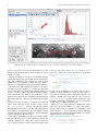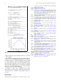
1
Proceedings of the 12th Python in Science Conference June 24 - June 29 • Austin, Texas Stéfan van der Walt Jarrod Millman Katy Huff P ROCEEDINGS OF THE 12 TH P YTHON IN S CIENCE C ONFERENCE Edited by Stéfan van der Walt, Jarrod Millman, and Katy Huff. SciPy 2013 Austin, Texas June 24 - June 29, 2013 c 2013. The articles in the Proceedings of the Python in Science Conference are copyrighted and owned Copyright by their original authors This is an open-access publication and is distributed under the terms of the Creative Commons Attribution License, which permits unrestricted use, distribution, and reproduction in any medium, provided the original author and source are credited. For more information, please see: http://creativecommons.org/licenses/by/3.0/ ISBN-13: value O RGANIZATION Conference Chairs A NDY T ERREL, University of Texas J ONATHAN R OCHER, Enthought, Inc. Program Committee Chairs K ATY H UFF, University of Wisconsin and Argonne National Laboratory M ATT M C C ORMICK, Kitware, Inc. Tutorial Chairs D HARHAS P OTHINA, Texas Water Development Board F RANCESC A LTED, Continuum Analytics Sprint Chairs C ORRAN W EBSTER, Enthought, Inc. P ETER WANG, Continuum Analytics Birds-of-a-Feather (BoF) Chairs K YLE M ANDLI, University of Texas M ATTHEW T URK, Columbia University Communications Chairs A NTHONY S COPATZ, University of Chicago M AJKEN T RANBY, Enthought, Inc. Financial Aid Chairs J EFF D AILY, Pacific Northwest National Laboratory J OHN W IGGINS, Enthought, Inc. Operations Chair L EAH J ONES, Enthought, Inc. Sponsor Chair B RETT M URPHY, Enthought, Inc. Financial Chair B ILL C OWAN, Enthought, Inc. Mini-symposium Chairs T OM A LDCROFT, Harvard/Smithsonian Center for Astrophysics B RAD C HAPMAN, Bioinformatics Core, Harvard School of Public Health K ELSEY J ORDAHL, Enthought, Inc. G AEL VAROQUAUX, INRIA C HRIS B ARKER ,, National Oceanic and Atmospheric Administration Program Committee A RON A HMADIA T OM A LDCROFT C HRIS B ARKER N ATHAN B ELL J OSHUA B LOOM M ATTHEW B RETT B RAD C HAPMAN M ATT D AVIS D ANIEL D YE S ATRAJIT G HOSH P ERRY G REENFIELD K ELSEY J ORDAHL M ATTHEW K NEPLEY J ESSICA L U H ILARY M ASON M IKE M C K ERNS Z AIN M EMON A RONNE M ERRELLI S HELIA M IGUEZ A UGUST M UENCH C AIT P ICKENS S ERGE R EY T OM R OBITAILLE D AN S CHULT R ICH S IGNELL W ILLIAM S POTZ M ATT T ERRY E RIK T OLLERUD J AMES T URNER G ERALDINE VAN DER A UWERA J AKE VAN DER P LAS G AEL VAROQUAX P ETER WANG A NDREW W ILSON Program Staff J ODI H AVRANEK, Enthought, Inc. J IM I VANOFF, Enthought, Inc. L AUREN J OHNSON, Enthought, Inc. O UTSTANDING S PONSORSHIP R ECIPIENTS D AMI ÁN AVILA J OSHUA C ARP C ARLOS C ORDOBA M ARIANNE C ORVELLEC S ERGE G UELTON K ATY H UFF U RSULA I TURRARAN -V IVEROS A ARON M EURER S TUART M UMFORD S AM P ORTNOW S AM P ORTNOW J OON R O M ATTHEW R OCKLIN J OSHUA WARNER C ONTENTS Preface 1 Andy Terrel, Jonathan Rocher DMTCP: Bringing Checkpoint-Restart to Python 2 Kapil Arya, Gene Cooperman Multidimensional Data Exploration with Glue 8 Christopher Beaumont, Thomas Robitaille, Alyssa Goodman, Michelle Borkin Hyperopt: A Python Library for Optimizing the Hyperparameters of Machine Learning Algorithms 13 James Bergstra, Dan Yamins, David D. Cox SkData: Data Sets and Algorithm Evaluation Protocols in Python 21 James Bergstra, Nicolas Pinto, David D. Cox Using Python to Study Rotational Velocity Distributions of Hot Stars 28 Gustavo Bragança, Simone Daflon, Katia Cunha, Thomas Bensby, Sally Oey, Gregory Walth Automating Quantitative Confocal Microscopy Analysis 33 Mark E. Fenner, Barbara M. Fenner Detection and characterization of interactions of genetic risk factors in disease 40 Patricia Francis-Lyon, Shashank Belvadi, Fu-Yuan Cheng Pythran: Enabling Static Optimization of Scientific Python Programs 46 Serge Guelton, Pierrick Brunet, Alan Raynaud, Adrien Merlini, Mehdi Amini Adapted G-mode Clustering Method applied to Asteroid Taxonomy 53 Pedro Henrique Hasselmann, Jorge Márcio Carvano, Daniela Lazzaro Ginga: an open-source astronomical image viewer and toolkit 61 Eric Jeschke Exploring Collaborative HPC Visualization Workflows using VisIt and Python 69 Hari Krishnan, Cyrus Harrison, Brad Whitlock, David Pugmire, Hank Childs SunPy: Python for Solar Physicists 74 Stuart Mumford, David Pérez-Suárez, Steven Christe, Florian Mayer, Russell J. Hewett Reproducible Documents with PythonTeX 78 Geoffrey M. Poore lpEdit: an editor to facilitate reproducible analysis via literate programming 85 Adam J Richards, Andrzej S. Kosinski, Camille Bonneaud, Delphine Legrand, Kouros Owzar GraphTerm: A notebook-like graphical terminal interface for collaboration and inline data visualization 90 Ramalingam Saravanan Modeling the Earth with Fatiando a Terra Leonardo Uieda, Vanderlei C. Oliveira Jr, Valéria C. F. Barbosa 96 PROC. OF THE 12th PYTHON IN SCIENCE CONF. (SCIPY 2013) 1 Preface Andy Terrel∗† , Jonathan Rocher‡ F SciPy 2013, the twelfth annual Scientific Computing with Python conference, was held June 24th-29th 2013 in Austin, Texas, USA. SciPy is a community dedicated to the advancement of scientific computing through open source Python software for mathematics, science, and engineering. The annual SciPy Conference allows participants from academic, commercial, and governmental organizations to showcase their newest tools and technics, learn from skilled users and developers, and collaborate on code development. These tools most often involve lower level languages but are characterized by a common goal of exposing most functionalities to Python users to maximize efficiency and simplicity of usage. This 12th edition has seen an amazing surge in attendance, with people from 5 continents, while retaining the great collaborative and friendly atmosphere that has characterized SciPy conferences over the years. Among many other improvements, this edition has seen a big push in making the proceedings of higher quality, available more quickly to the community, and better recognized. We encourage you to learn from these papers as well as the corresponding videos of the talks at http://conference.scipy.org/scipy2013 If you were able to attend SciPy2013, we hope this conference has been fruitful professionally, allowing you to expand your knowledge and network. And even if you were not able to join us this year, we hope to see you in 2014! For the SciPy2013 organizers, Andy Terrel and Jonathan Rocher, chairs of SciPy2013 * Corresponding author: [email protected] † University of Texas at Austin ‡ Enthought, Inc. c 2013 Andy Terrel et al. This is an open-access article distributed Copyright ○ under the terms of the Creative Commons Attribution License, which permits unrestricted use, distribution, and reproduction in any medium, provided the original author and source are credited. 2 PROC. OF THE 12th PYTHON IN SCIENCE CONF. (SCIPY 2013) DMTCP: Bringing Checkpoint-Restart to Python Kapil Arya∗† , Gene Cooperman† http://www.youtube.com/watch?v=1l_wGZz0JEE F Abstract—DMTCP (Distributed MultiThreaded CheckPointing) is a mature checkpoint-restart package. It operates in user-space without kernel privilege, and adapts to application-specific requirements through plugins. While DMTCP has been able to checkpoint Python and IPython "from the outside" for many years, a Python module has recently been created to support DMTCP. IPython support is included through a new DMTCP plugin. A checkpoint can be requested interactively within a Python session, or under the control of a specific Python program. Further, the Python program can execute specific Python code prior to checkpoint, upon resuming (within the original process), and upon restarting (from a checkpoint image). Applications of DMTCP are demonstrated for: (i) Python-based graphics using VNC; (ii) a Fast/Slow technique to use multiple hosts or cores to check one Cython computation in parallel; and (iii) a reversible debugger, FReD, with a novel reverse-expression watchpoint feature for locating the cause of a bug. Index Terms—checkpoint-restart, DMTCP, IPython, Cython, reversible debugger Introduction DMTCP (Distributed MultiThreaded CheckPointing) [Ansel09] is a mature user-space checkpoint-restart package. One can view checkpoint-restart as a generalization of pickling. Instead of saving an object to a file, one saves the entire Python session to a file. Checkpointing graphics in Python is also supported—by checkpointing a virtual network client (VNC) session with Python running inside that session. DMTCP is available as a Linux package for many popular Linux distributions. DMTCP can checkpoint Python or IPython from the outside, i.e. by treating Python as a black box. To enable checkpointing, the Python interpreter is launched in the following manner: $ dmtcp_checkpoint python <args> $ dmtcp_command --checkpoint The command dmtcp_command can be used at any point to create a checkpoint of the entire session. However, most Python programmers will prefer to request a checkpoint interactively within a Python session, or else programmatically from inside a Python or Cython program. DMTCP is made accessible to Python programmers as a Python module. Hence, a checkpoint is executed as import dmtcp; dmtcp.checkpoint(). This Python * Corresponding author: [email protected] † Northeastern University c 2013 Kapil Arya et al. This is an open-access article distributed Copyright ○ under the terms of the Creative Commons Attribution License, which permits unrestricted use, distribution, and reproduction in any medium, provided the original author and source are credited. module provides this and other functions to support the features of DMTCP. The module for DMTCP functions equally well in IPython. This DMTCP module implements a generalization of a saveWorkspace function, which additionally supports graphics and the distributed processes of IPython. In addition, three novel uses of DMTCP for helping debug Python are discussed. 1. Fast/Slow Computation—Cython provides both traditional interpreted functions and compiled C functions. Interpreted functions are slow, but correct. Compiled functions are fast, but users sometimes declare incorrect C types, causing the compiled function silently return a wrong answer. The idea of fast/slow computation is to run the compiled version on one computer node, while creating checkpoint images at regular intervals. Separate computer nodes are used to check each interval in interpreted mode between checkpoints. 2. FReD—a Fast Reversible Debugger that works closely with the Python pdb debugger, as well as other Python debuggers. 3. Reverse Expression Watchpoint—This is a novel feature within the FReD reversible debugger. Assume a bug occurred in the past. It is associated with the point in time when a certain expression changed. Bring the user back to a pdb session at the step before the bug occurred. The remaining sections describe: the DMTCP-Python Integration through a Python Module; and several extensions of the integration of DMTCP with Python. The extensions include support for Checkpointing Python-Based Graphics; Checking Cython with Multiple CPython Instances (fast/slow technique); and Reversible Debugging with FReD. More information about DMTCP is added in Appendix: Background of DMTCP. DMTCP-Python Integration through a Python Module A Python module, dmtcp.py, has been created to support checkpointing both from within an interactive Python/IPython session and programmatically from within a Python or Cython program. DMTCP has been able to asynchronously generate checkpoints of a Python session for many years. However, most users prefer the more fine-grained control of a Python programmatic interface to DMTCP. This allows one to avoid checkpointing in the middle of a communication with an external server or other atomic transaction. DMTCP: BRINGING CHECKPOINT-RESTART TO PYTHON A Python Module to Support DMTCP Some of the features of module.py are best illustrated through an example. Here, a checkpoint request is made from within the application. ... import dmtcp ... # Request a checkpoint if running under checkpoint # control dmtcp.checkpoint() # Checkpoint image has been created ... It is also easy to add pre- and post-checkpoint processing actions. ... import dmtcp ... def my_ckpt(<args>): # Pre processing my_pre_ckpt_hook(<args>) ... # Create checkpoint dmtcp.checkpoint() # Checkpoint image has been created ... if dmtcp.isResume(): # The process is resuming from a checkpoint my_resume_hook(<args>) ... else: # The process is restarting from a previous # checkpoint my_restart_hook(<args>) ... return ... The function my_ckpt can be defined in the application by the user and can be called from within the user application at any point. Extending the DMTCP Module for Managing Sessions These core checkpoint-restart services are further extended to provide the user with the concept of multiple sessions. A checkpointed Python session is given a unique session id to distinguish it from other sessions. When running interactively, the user can view the list of available checkpointed sessions. The current session can be replaced by any of the existing session using the session identifier. The application can programmatically revert to an earlier session as shown in the following example: ... import dmtcp ... sessionId1 = dmtcp.checkpoint() ... sessionId2 = dmtcp.checkpoint() ... ... if <condition>: dmtcp.restore(sessionId2) else: dmtcp.restore(sessionId1) 3 in user’s home directory. During restart, if the configuration files are missing, the restarted computation may fail to continue. Thus, DMTCP must checkpoint and restore all the files required for proper restoration of an IPython session. Attempting to restore all configuration files during restart poses yet another problem: the existing configuration files might have newer contents. Overwriting these newer files with copies from the checkpoint time may result in the loss of important changes. To avoid overwriting the existing configuration files, the files related to IPython session are restored in a temporary directory. Whenever IPython shell attempts to open a file in the original configuration directory, the filepath is updated to point to the temporary directory. Thus, the files in the original configuration directory are never modified. Further, the translation from original to temporary path is transparent to the IPython shell. Save-Restore for Parallel IPython Sessions DMTCP is capable of checkpointing a distributed computations with processes running on multiple nodes. It automatically checkpoints and restores various kinds of inter-process communication mechanisms such as shared-memory, message queues, pseudo-ttys, pipes and network sockets. An IPython session involving a distributed computation running on a cluster is checkpointed as a single unit. DMTCP allows restarting the distributed processes in a different configuration than the original. For example, all the processes can be restarted on a single computer for debugging purposes. In another example, the computation may be restarted on a different cluster altogether. Checkpointing Python-Based Graphics Python is popular for scientific visualizations. It is possible to checkpoint a Python session with active graphics windows by using VNC. DMTCP supports checkpoint-restart of VNC server. In this case, a VNC server can be started automatically. The process environment is modified to allow the Python interpreter to communicate with the VNC server instead of the X-window server. For visualization, a VNC client can be fired automatically to display the graphical window. During checkpoint, the VNC server is checkpointed as part of the computation, while the VNC client is not. During restart, the Python session and the VNC server are restored from their checkpoint images, and a fresh VNC client is launched. This VNC client communicates with the restored server and displays the graphics to the end user. ... import dmtcp ... # Start VNC server dmtcp.startGraphics() ... Save-Restore for IPython Sessions # Start VNC viewer dmtcp.showGraphics() To checkpoint an IPython session, one must consider the configuration files. The configuration files are typically stored # generate graphics (will be shown in the VNC viewer) ... 4 To understand the algorithm behind the code, we recall some VNC concepts. X-window supports multiple virtual screens. A VNC server creates a new virtual screen. The graphics contained in the VNC server is independent of any X-window screen. The VNC server process persists as a daemon. A VNC viewer displays a specified virtual screen in a window in a console. When python generates graphics, the graphics is sent to a virtual screen specified by the environment variable $DISPLAY. The command dmtcp.startGraphics() creates a new X-window screen by creating a new VNC server and sets the $DISPLAY environment variable to the new virtual screen. All python graphics are now sent to this new virtual screen. The additional screen is invisible to the python user until the python command dmtcp.showGraphics() is given. The Python Command dmtcp.showGraphics() operates by invoking a VNC viewer. At the time of checkpoint, the VNC server process is checkpointed along with the python interpretor while the VNC viewer is not checkpointed. On restart, the VNC server detects the stale connection to the old VNC viewers. The VNC server perceives this as the VNC viewer process that has now died. The DMTCP module then launches anew VNC viewer to connect to the VNC server. Checking Cython with Multiple CPython Instances A common problem for compiled versions of Python such as Cython [Behnel10] is how to check whether the compiled computation is faithful to the interpreted computation. Compilation errors can occur if the compiled code assumes a particular C type, and the computation violates that assumption for a particular input. Thus, one has to choose between speed of computation and a guarantee that that the compiled computation is faithful to the interpreted computation. A typical scenario might be a case in which the compiled Cython version ran for hours and produced an unexpected answer. One wishes to also check the answer in a matter of hours, but pure Python (CPython) would take much longer. Informally, the solution is known as a fast/slow technique. There is one fast process (Cython), whose correctness is checked by multiple slow processes (CPython). The core idea is to run the compiled code, while creating checkpoint images at regular intervals. A compiled computation interval is checked by copying the two corresponding checkpoints (at the beginning and end of the interval) to a separate computer node for checking. The computation is restarted from the first checkpoint image, on the checking node. But when the computation is first restarted, the variables for all user Python functions are set to the interpreted function object. The interval of computation is then re-executed in interpreted mode until the end of the computation interval. The results at the end of that interval can then be compared to the results at the end of the same interval in compiled mode. Figure 1 illustrates the above idea. A similar idea has been used by [Ghoshal11] for distributed speculative parallelization. Note that in order to compare the results at the end of a computation interval, it is important that the interpreted PROC. OF THE 12th PYTHON IN SCIENCE CONF. (SCIPY 2013) Fig. 1: Fast Cython with Slow CPython "checking" nodes. version on the checker node stop exactly at the end of the interval, in order to compare with the results from the checkpoint at the end of the same interval. The simplest way to do this is to add a counter to a frequently called function of the end-user code. The counter is incremented each time the function is called. When the counter reaches a pre-arranged multiple (for example, after every million calls), the compiled version can generate a checkpoint and write to a file the values of variables indicating the state of the computation. The interpreted version writes to a file the values of variables indicating its own state of the computation. mycounter = 0 def freq_called_user_fnc(<args>): global mycounter mycounter += 1 if mycounter % 1000000 == 0: # if running as Cython: if type(freq_called_user_fnc) == type(range): # write curr. program state to cython.log dmtcp.checkpoint() if dmtcp.isRestart(): # On restart from ckpt image, # switch to pure Python. else: # else running as pure Python # write curr. program state to purePython.log sys.exit(0) ... # original body of freq_called_user_fnc return The above code block illustrates the principles. One compares cython.log and purePython.log to determine if the compiled code was faithful to the interpreted code. If the Cython code consists of direct C calls between functions, then it will also be necessary to modify the functions of the C code generated by Cython, to force them to call the pure Python functions on restart after a checkpoint. Reversible Debugging with FReD While debugging a program, often the programmer over steps and has to restart the debugging session. For example, while debugging a program, if the programmer steps over (by issue next command inside the debugger) a function f() only to determine that the bug is in function f() itself, he or she is left with no choice but to restart from the beginning. Reversible debugging is the capability to run an application "backwards" in time inside a debugger. If the programmer detects that the problem is in function f(), instead of restarting from the beginning, the programmer can issue a reverse-next command which takes it to the previous DMTCP: BRINGING CHECKPOINT-RESTART TO PYTHON 5 Fig. 4: Reverse Expression Watchpoint. More complex reverse commands Fig. 2: Fast Reversible Debugger. Fig. 3: Reverse Commands. step. He or she can then issue a step command to step into the function in order to find the problem. FReD (Fast Reversible Debugger) [Arya12], [FReD13] is a reversible debugger based on checkpoint-restart. FReD is implemented as a set of Python scripts and uses DMTCP to create checkpoints during the debugging session. FReD also keeps track of the debugging history. Figure 2 shows the architecture of FReD. A Simple UNDO Command The UNDO command reverses the effect of a previous debugger command such as next, continue or finish. This is the most basic of reversible debugging commands. The functionality of the UNDO command for debugging Python is trivially implemented. A checkpoint is taken at the beginning of the debugging session and a list of all debugging commands issued since the checkpoint are recorded. To execute the UNDO command, the debugging session is restarted from the checkpoint image, and the debugging commands are automatically re-executed from the list excluding the last command. This takes the process back to before the debugger command was issued. In longer debugging sessions, checkpoints are taken at frequent intervals to reduce the time spent in replaying the debugging history. Figure 3 shows some typical debugging commands being executed in forward as well as backward direction in time. Suppose that the debugging history appears as [next,next] i.e. the user issued two next commands. Further, the second next command stepped over a function f(). Suppose further that FReD takes checkpoints before each of these commands. In this situation, the implementation for reverse-next command is trivial: one restarts from the last checkpoint image. However, if the command issued were reverse-step, simply restarting from the previous checkpoint would not suffice. In this last case, the desired behavior is to take the debugger to the last statement of the function f(). In such a situation one needs to decompose the last command into a series of commands. At the end of this decomposition, the last command in the history is a step. At this point, the history may appear as: [next,step,next, ...,next,step]. The process is then restarted from the last checkpoint and the debugging history is executed excluding the last step command. Decomposing a command into a series of commands terminating with step is non-trivial, and an algorithm for that decomposition is presented in [Visan11] . A typical debugging session in FReD with Python: $ fredapp.py python -mpdb a.py (Pdb) break main (Pdb) run (Pdb) fred-checkpoint (Pdb) break 6 (Pdb) continue (Pdb) fred-history [break 6, continue] (Pdb) fred-reverse-next (Pdb) fred-history [break 7, next, next, next, next, next, next, next, next, next, next, step, next, next, next, where] Reverse Expression Watchpoints The reverse expression watchpoint automatically finds the location of the fault for a given expression in the history of the program execution. It brings the user directly to a statement (one that is not a function call) at which the expression is correct, but executing the statement will cause the expression to become incorrect. Figure 4 provides a simple example. Assume that a bug occurs whenever a linked list has length longer than one million. So an expression linked_list.len() <= 1000000 is assumed to be true throughout. Assume that it is too expensive to frequently compute the length of the linked list, since this 6 would require O(n2 ) time in what would otherwise be a O(n) time algorithm. (A more sophisticated example might consider a bug in an otherwise duplicate-free linked list or an otherwise cycle-free graph. But the current example is chosen for ease of illustrating the ideas.) If the length of the linked list is less than or equal to one million, we will call the expression "good". If the length of the linked list is greater than one million, we will call the expression "bad". A "bug" is defined as a transition from "good" to "bad". There may be more than one such transition or bug over the process lifetime. Our goal is simply to find any one occurrence of the bug. The core of a reverse expression watchpoint is a binary search. In Figure 4, assume a checkpoint was taken near the beginning of the time interval. So, we can revert to any point in the illustrated time interval by restarting from the checkpoint image and re-executing the history of debugging commands until the desired point in time. Since the expression is "good" at the beginning of Figure 4 and it is "bad" at the end of that figure, there must exist a buggy statement—a statement exhibiting the transition from "good" to "bad". A standard binary search algorithm converges to a case in which the current statement is "good" and the next statement transitions from "good" to "bad". By the earlier definition of a "bug", FReD has found a statement with a bug. This represents success. If implemented naively, this binary search requires that some statements may need to be re-executed up to log2 N times. However, FReD can also create intermediate checkpoints. In the worst case, one can form a checkpoint at each phase of the binary search. In that case, no particular subinterval over the time period needs to be executed more than twice. A typical use of reverse-expression-watchpoint: $ ./fredapp.py python -mpdb ./autocount.py -> import sys, time (Pdb) break 21 Breakpoint 1 at /home/kapil/fred/autocount.py:21 (Pdb) continue > /home/kapil/fred/autocount.py(21)<module>() # Required for fred-reverse-watch (Pdb) fred-checkpoint (Pdb) break 28 Breakpoint 2 at /home/kapil/fred/autocount.py:28 (Pdb) continue ... <program output> ... > /home/kapil/fred/autocount.py(28)<module>() (Pdb) print num 10 (Pdb) fred-reverse-watch num < 5 (Pdb) print num 4 (Pdb) next (Pdb) print num 5 Conclusion DMTCP is a widely used standalone checkpoint-restart package. We have shown that it can be closely integrated with Python. Specifically, parallel sessions with IPython, alternating interpreted and compiled execution modes, graphics, and enhancing Python debugger with reversibility. The implementation can be extended by the end users to augment PROC. OF THE 12th PYTHON IN SCIENCE CONF. (SCIPY 2013) Fig. 5: Architecture of DMTCP. the capabilities of Python beyond the simple example of checkpoint-restart. Acknowledgment This work was partially supported by the National Science Foundation under Grant OCI-0960978. Appendix: Background of DMTCP DMTCP [Ansel09] is a transparent checkpoint-restart package with its roots going back eight years [Rieker06]. It works completely in user space and does not require any changes to the application or the operating system. DMTCP can be used to checkpoint a variety of user applications including Python. Using DMTCP to checkpoint an application is as simple as executing the following commands: dmtcp_checkpoint ./a.out dmtcp_command -c ./dmtcp_restart_script.sh DMTCP automatically tracks all local and remote child processes and their relationships. As seen in Figure 5, a computation running under DMTCP consists of a centralized coordinator process and several user processes. The user processes may be local or distributed. User processes may communicate with each other using sockets, shared-memory, pseudo-terminals, etc. Further, each user process has a checkpoint thread which communicates with the coordinator. DMTCP Plugins DMTCP plugins are used to keep DMTCP modular. There is a separate plugin for each operating system resource. Examples of plugins are pid plugin, socket plugin, and file plugin. Plugins are responsible for checkpointing and restoring the state of their corresponding resources. The execution environment can change between checkpoint and restart. For example, the computation might be restarted on a different computer which has different file mount points, a DMTCP: BRINGING CHECKPOINT-RESTART TO PYTHON 7 Checkpoint On receiving the checkpoint request from the coordinator, the checkpoint thread sends the checkpoint signal to all the user threads of the process. This quiesces the user threads by forcing them to block inside a signal handler, defined by the DMTCP. The checkpoint image is created by writing all of user-space memory to a checkpoint image file. Each process has its own checkpoint image. Prior to checkpoint, each plugin will have copied into user-space memory any kernel state associated with its concerns. Examples of such concerns include network sockets, files, and pseudo-terminals. Once the checkpoint image has been created, the checkpoint thread "un-quiesces" the user threads and they resume executing application code. At the time of checkpoint, all of user-space memory is written to a checkpoint image file. The user threads are then allowed to resume execution. Note that user-space memory includes all of the run-time libraries (libc, libpthread, etc.), which are also saved in the checkpoint image. In some cases, state outside the kernel must be saved. For example, in handling network sockets, data in flight must be saved. This is done by draining the network data by sending a special cookie through the "send" end of each socket in one phase. In a second phase, after a global barrier, data is read from the "receive" end of each socket until the special cookie is received. The in-flight data has now been copied into user-space memory, and so will be included in the checkpoint image. On restart, the network buffers are refilled by sending the in-flight data back to the peer process, which then sends the data back into the network. Fig. 6: DMTCP Plugins. different network address, etc. Plugins handle such changes in the execution environment by virtualizing these aspects. Figure 6 shows the layout of DMTCP plugins within the application. DMTCP Coordinator DMTCP uses a stateless centralized process, the DMTCP coordinator, to synchronize checkpoint and restart between distributed processes. The user interacts with the coordinator through the console to initiate checkpoint, check the status of the computation, kill the computation, etc. It is also possible to run the coordinator as a daemon process, in which case, the user may communicate with the coordinator using the command dmtcp_command. Checkpoint Thread The checkpoint thread waits for a checkpoint request from the DMTCP coordinator. On receiving the checkpoint request, the checkpoint thread quiesces the user threads and creates the checkpoint image. To quiesce user threads, it installs a signal handler for a dedicated POSIX signal (by default, SIGUSR2). Once the checkpoint image has been created, the user threads are allowed to resume executing application code. Similarly, during restart, once the process memory has been restored, the user threads can resume executing application code. Restart As the first step of restart phase, all memory areas of the process are restored. Next, the user threads are recreated. The plugins then receive the restart notification and restore their underlying resources, translation tables, etc. Finally, the checkpoint thread "un-quiesces" the user threads and the user threads resume executing application code. R EFERENCES [Ansel09] Jason Ansel, Kapil Arya, and Gene Cooperman. DMTCP: Transparent Checkpointing for Cluster Computations and the Desktop, 23rd IEEE International Symposium on Parallel and Distributed Processing (IPDPS-09), 1-12, 2009 http://dmtcp. sourceforge.net/. [Arya12] Kapil Arya, Tyler Denniston, Ana Maria Visan, and Gene Cooperman. FReD: Automated Debugging via Binary Search through a Process Lifetime, http://arxiv.org/abs/1212.5204. [FReD13] FReD (Fast Reversible Debugger) Software. https://github.com/ fred-dbg/fred [Behnel10] R. Bradshaw, S. Behnel, D. S. Seljebotn, G. Ewing, et al. Cython: The Best of Both Worlds, Computing in Science Engineering, 2010. [Ghoshal11] Devarshi Ghoshal, Sreesudhan R. Ramkumar, and Arun Chauhan. Distributed Speculative Parallelization using Checkpoint Restart, Procedia Computer Science, 2011. [Rieker06] Michael Rieker, Jason Ansel, and Gene Cooperman. Transparent User-Level Checkpointing for the Native POSIX Thread Library for Linux, Proceeding of PDPTA-06, 492-498, 2006. [Visan11] Ana-Maria Visan, Kapil Arya, Gene Cooperman, and Tyler Denniston. URDB: A Universal Reversible Debugger Based on Decomposing Debugging Histories, In Proc. of 6th Workshop on Programming Languages and Operating Systems (PLOS’2011) (part of Proc. of 23rd ACM SOSP), 2011. 8 PROC. OF THE 12th PYTHON IN SCIENCE CONF. (SCIPY 2013) Multidimensional Data Exploration with Glue Christopher Beaumont∗† , Thomas Robitaille‡ , Alyssa Goodman§ , Michelle Borkin§ http://www.youtube.com/watch?v=47LNpvDlKUk F Abstract—Modern research projects incorporate data from several sources, and new insights are increasingly driven by the ability to interpret data in the context of other data. Glue is an interactive environment built on top of the standard Python science stack to visualize relationships within and between datasets. With Glue, users can load and visualize multiple related datasets simultaneously. Users specify the logical connections that exist between data, and Glue transparently uses this information as needed to enable visualization across files. This functionality makes it trivial, for example, to interactively overplot catalogs on top of images. The central philosophy behind Glue is that the structure of research data is highly customized and problem-specific. Glue aims to accommodate this and simplify the "data munging" process, so that researchers can more naturally explore what their data have to say. The result is a cleaner scientific workflow, faster interaction with data, and an easier avenue to insight. Index Terms—data visualization, exploratory data analysis, Python Introduction The world is awash in increasingly accessible and increasingly interrelated data. Modern researchers rarely consider data in isolation. In astronomy, for example, researchers often complement newly-collected data with publicly-available survey data targeting a different range of the electromagnetic spectrum. Because of this, new discoveries are increasingly dependent upon interpreting data in the context of other data. Unfortunately, most of the current interactive tools for data exploration focus on analyzing a single dataset at a time. It is considerably more difficult to explore several conceptually related datasets at once. Scientists typically resort to noninteractive techniques (e.g., writing scripts to produce static visualizations). This slows the pace of investigation, and makes it difficult to uncover subtle relationships between datasets. To address this shortcoming, we have been developing Glue. Glue is an interactive data visualization environment that focuses on multi-dataset exploration. Glue allows users to specify how different datasets are related, and uses this information to dynamically link and overlay visualizations of several datasets. Glue also integrates into Python-based analysis workflows, and eases the back-and-forth between interactive and non-interactive data analysis. * Corresponding author: [email protected] † University of Hawaii, Harvard University ‡ Max Planck Institute for Astronomy § Harvard University c 2013 Christopher Beaumont et al. This is an open-access article Copyright ○ distributed under the terms of the Creative Commons Attribution License, which permits unrestricted use, distribution, and reproduction in any medium, provided the original author and source are credited. The Basic Glue Workflow The central visualization philosophy behind Glue is the idea of linked views -- that is, multiple related representations of a dataset that are dynamically connected, such that interaction with one view affects the appearance of another. For example, a user might create two different scatter plots of a multidimensional table, select a particular region of parameter space in one plot, and see the points in that region highlighted in both plots. Linked-view visualizations are especially effective at exploring high-dimensional data. Glue extends this idea to related data sets spread across multiple files. Let’s illustrate the basic Glue workflow with an example. An astronomer is studying Infrared Dark Clouds (environments of star formation) in our Galaxy. Her data sets include a catalog of known Infrared Dark Clouds, a second catalog of "cores" (substructures embedded in these clouds where the stars actually form), and a wide-field infrared survey image of a particular cloud. Step 1 She begins by loading the cloud catalog into Glue. She creates a scatter plot of the position of each cloud, as well as a histogram showing the distribution of surface densities. She creates each visualization by dragging the data item onto the visualization area. At this point, her screen looks like Figure 1. Step 2 She is interested in a particular region of the sky, and thus draws a lasso around particular points in the scatter plot. This creates a new "subset", which is shown in red on each visualization (Figure 2). If she traces a different region on either plot, the subset will update in both views automatically. Step 3 Next she loads the infrared image. She would like to see how the points in the catalog relate to structures in the image, by overplotting the subset on the image. To do this, she first "links" the data by defining the logical relationships between the two files. She opens a data linking dialog, which displays the attributes defined for each dataset (Figure 3). The image has attributes for the x and y location of each pixel, and the catalog has columns which list the location of each object in the same coordinate system. She highlights the attribute describing the x location attribute for each dataset (Right Ascension), and "links" them (in effect informing Glue that the two attributes describe the same quantity). She repeats this for the y location attribute (declination), and closes the dialog. Step 4 Now, she can drag the subset onto the image, to overplot these points at their proper location (this is possible MULTIDIMENSIONAL DATA EXPLORATION WITH GLUE Fig. 1: The basic Glue interface, shown at the end of step 1. Datasets are listed on the left panel. Dragging them to the right creates a new visualization. because Glue now has enough information to compute the location of each catalog source in the image. The details of how this is accomplished are described in the next section). All three plots are still linked: if the user highlights a new region in the image, this will redefine the subset and update each plot. Figure 4 shows the Glue interface at this point. The relationship between the catalog and image was very simple; each dataset described the same spatial quantities, in the same units. In general, connections between datasets are more complicated. For example, the catalog of cores specifies positions in a different coordinate system. Because of this, Glue allows users to connect quantities across datasets using transformation functions. Glue includes some of these functions by default, but users can also write their own functions for arbitrary transformations. Glue uses these functions as needed to transform quantities between coordinate systems, to correctly overlay visualizations and/or filter data in subsets. Step 5 Our scientist discovers several interesting relationships between these datasets -- in particular, that several distinct entries in the cloud catalog appear to form a coherent, extended structure in the image. Furthermore, the cores embedded in these clouds all have similar velocities, strengthening the argument that they are related. At this point, she decides to test this hypothesis more rigorously, by comparing to models of structure formation. This analysis will happen outside of Glue. She saves all of her subsets as masks, for followup analysis. Furthermore, she saves the entire Glue session, which allows her to re-load these datasets, dataset 9 Fig. 2: Glue after step 2. Tracing a cluster of points in the scatter plot creates a new subset, The histogram plot updates automatically. Fig. 3: The dialog for expression relationships between different datasets in step 3. Here, both datasets use the same spatial coordinates. connections, and subset definitions at any time. Glue Architecture The scenario above outlines the basic workflow that Glue enables -- Glue allows users to create interactive linked visualizations, and to drill down into interesting subsets of these visualizations. One of the design priorities in Glue is to keep visualization code as simple and modular as possible, so that adding new visualizations is straightforward. Here we 10 PROC. OF THE 12th PYTHON IN SCIENCE CONF. (SCIPY 2013) Fig. 4: Once the catalog and image are linked, the user can overplot the original subset on the image (step 4). provide an overview of how we have implemented cross-data linking in Glue, while striving to keep visualization code as simple as possible. Keeping visualizations in-sync is accomplished with the publish/subscribe pattern. Glue defines several standard messages that communicate state changes (e.g., that a subset definition has been changed, a subset has been added or removed, etc.). Visualization clients attach callback methods to a central hub; these callback methods are meant to respond to a particular type of state change (e.g., to change the appearance of a plot). The hub is responsible for broadcasting messages it receives -- in effect, calling each callback function registered with a particular message. Thus, to stay synchronized, a visualization client simply needs to implement callback functions that handle each type of message, and register these with the hub. The hub receives messages to broadcast from data and subset objects. The base classes for these objects override the __setattribute__ method, such that state changes automatically send messages to the hub. This means that, in most situations, code that edits the state (for example, code that translates user-drawn regions-of-interest to subset definitions) need not manually broadcast messages. Glue enables data linking across files by providing a simple, dictionary-like interface for accessing attributes from data. For example, consider the case where a user overplots a catalog on top of an image. Such an overlay requires knowledge of the location of each catalog entry in the pixel coordinate system of the image. The pseudo-code for the overlay looks like this: def overplot_catalog(catalog_data): try: # try to fetch requested quantities x = catalog_data[’pixel_coord_x’] y = catalog_data[’pixel_coord_y’] except InvalidAttribute: # cannot compute pixel location of catalog return # x, y are numpy arrays plot(x, y) In other words, visualization code simply looks up the information it needs. Behind the scenes, the data object is responsible for retrieving and/or computing this quantity, and returning a NumPy array. If it cannot do this, it raises an InvalidAttribute exception, which visualization code responds to. Importantly, visualization code is not responsible for performing coordinate transformations. Subsets also rely on this interface for filtering data. Each subset stores its logical definition as a subset state. Fundamentally, subset states are combinations of inequalities. Each subset state has a to_mask method that is capable of filtering a given dataset. For example, the implementation of a simple inequality subset state looks like this: class GreaterThanSubsetState(SubsetState): def __init__(self, attribute, threshold): self.attribute = attribute self.threshold = threshold MULTIDIMENSIONAL DATA EXPLORATION WITH GLUE 11 translation functions presented in the data linking UI. This code can be put in a configuration file that glue runs on startup. Custom data loading A traditional weakness of GUIs is their fragility to unanticipated data formats. However, Glue allows users to specify custom data loader methods, to parse data in unrecognized formats. For example, to parse jpeg files: from glue.config import data_factory from glue.core import Data from skimage.io import imread @data_factory(’JPEG Reader’, ’*.jpg’) def read_jpeg_image(file_name): im = imread(file_name) return Data(label=’Image’, r=im[:, :, 0], g=im[:, :, 1], b=im[:, :, 2]) Fig. 5: Eventually, the user annotates several interesting regions in parameter space (step 5). These subsets can be exported as masks for further analysis. def to_mask(self, data): # uses the data dictionary interface return data[self.attribute] > self.threshold Because subset states retain the information about which quantities they constrain, they can be applied across datasets, provided the quantities that they filter against are defined or computable in the target dataset. Internally, Glue maintains a graph of coordinate transformation functions when the user defines connections between datasets. The nodes in this graph are all the attributes defined in all datasets, and the edges are translation functions. When client code tries to access a quantity that is not originally stored in a dataset, Glue searches for a path from quantities that are natively present to the requested quantity. If such a path exists, The relevant set of transformation functions are called, and the result is returned. Integrating with Python Workflows Python is the language-of-choice for many scientists, and the fact that Glue is written in Python means that it is more easily "hackable" than a typical GUI application. This blurs the boundary between interactive and scripted analysis, and can lead to a more fluid workflow. Here are several examples: Custom data linking functions Glue allows users to specify arbitrary Python functions to translate between quantities in different datasets. As a simple example, consider a function which translates between pounds and kilograms: from glue.config import link_function @link_function(info=’Convert pounds to kilograms’) def pounds2kilos(lbs): return lbs / 2.2 Link functions accept and return NumPy arrays. The link_function decorator adds this function to the list of This function parses a data object with three attributes (the red, green, and blue channels). The data_factory decorator adds this function to the data loading user interface. Setup Scripts Glue can be passed a Python script to run on startup. This can be a convenient way to automate the task of loading and linking several files that are frequently visualized. This addresses another typical pain-point of GUIs -- the repetitive mouse-clicking one has to do every time a GUI is restarted. Calling Glue from Python Glue can be invoked during a running Python session. Many scientists use Python for dataexploration from the command line (or, more recently, the IPython notebook). Glue can be used to interact with live Python variables. For example, Glue includes a convenience function, qglue, that composes "normal" data objects like NumPy arrays and Pandas DataFrames into Glue objects, and initializes the Glue UI with these variables. qglue is useful for quick questions about multidimensional data that arise midanalysis. Similarly, Glue embeds an IPython terminal that gives users access to the Python command line (and Glue variables) during a glue session. Variables in a Glue session can be introspected and analyzed on this command line. Relationship to Other Efforts Glue helps researchers uncover the relationships that exist between related datasets. It enables users to easily create multiple linked visualizations which can be used to identify and drill down into interesting data subsets. Many of the ideas behind Glue are rooted in previous efforts (for a more thorough history from an astronomy perspective, see [Goodman12]). The statistician John Tukey pioneered many of the ideas behind what he termed Exploratory Data Analysis (that is, the open-ended investigation of features in datasets, as distinguished from Confirmatory Data Analysis where specific hypotheses are tested systematically; [Tukey77]). In the early 1970s, he developed the PRIM-9 program, which implemented the idea of creating multiple views of multivariate data, and isolating data subsets. More modern linked-visualization programs influenced by PRIM-9 include GGobi, Spotfire, DataDesk, and Tableau (the first is free and open-source, the latter 3 are commercial). 12 Within the astronomy community, Topcat and Viewpoints focus on linked visualization of tabular data. Finally, some efforts from the Virtual Observatory community (especially the SAMP protocol) allow different visualization tools to interoperate, and hence provide a limited linked-view environment. Glue builds upon the ideas developed in these programs in a few key ways. The majority of these linked-view environments focus on the exploration of a single catalog. Glue generalizes this approach in two directions. First, Glue is designed to handle several files at a time, and to visually explore the connections between these files. Second, Glue handles nontabular data like images -- this is critical for applications in astronomy, medical imaging, and Geographic Information Systems. The landscape of data is evolving rapidly, and driving revolutions both within and beyond science. The phenomenon of "big data" is one of the most public facets of this revolution. Rapidly growing volumes of data present new engineering challenges for analysis, as well as new opportunities for datadriven decision making. Glue tackles a different but equally important facet of the data revolution, which we call "wide data". Data are becoming increasingly inter-related, and the ability to tease out these connections will enable new discoveries. Glue is a platform for visually and flexibly exploring these relationships. R EFERENCES [Goodman12] Goodman, Alyssa Principles of high-dimensional data visualization in astronomy Astronomische Nachrichten, Vol. 333, Issue 5-6, p.505 [Tukey77] Tukey, John Exploratory Data Analysis Addison-Wesley Publishing Company, 1977 PROC. OF THE 12th PYTHON IN SCIENCE CONF. (SCIPY 2013) PROC. OF THE 12th PYTHON IN SCIENCE CONF. (SCIPY 2013) 13 Hyperopt: A Python Library for Optimizing the Hyperparameters of Machine Learning Algorithms James Bergstra∗† , Dan Yamins‡ , David D. Cox§ http://www.youtube.com/watch?v=Mp1xnPfE4PY F Abstract—Sequential model-based optimization (also known as Bayesian optimization) is one of the most efficient methods (per function evaluation) of function minimization. This efficiency makes it appropriate for optimizing the hyperparameters of machine learning algorithms that are slow to train. The Hyperopt library provides algorithms and parallelization infrastructure for performing hyperparameter optimization (model selection) in Python. This paper presents an introductory tutorial on the usage of the Hyperopt library, including the description of search spaces, minimization (in serial and parallel), and the analysis of the results collected in the course of minimization. The paper closes with some discussion of ongoing and future work. Index Terms—Bayesian optimization, hyperparameter optimization, model selection Introduction Sequential model-based optimization (SMBO, also known as Bayesian optimization) is a general technique for function optimization that includes some of the most call-efficient (in terms of function evaluations) optimization methods currently available. Originally developed for experiment design (and oil exploration, [Mockus78]) SMBO methods are generally applicable to scenarios in which a user wishes to minimize some scalar-valued function f (x) that is costly to evaluate, often in terms of time or money. Compared with standard optimization strategies such as conjugate gradient descent methods, model-based optimization algorithms invest more time between function evaluations in order to reduce the number of function evaluations overall. The advantages of SMBO are that it: • leverages smoothness without analytic gradient, • handles real-valued, discrete, and conditional variables, • handles parallel evaluations of f (x), • copes with hundreds of variables, even with budget of just a few hundred function evaluations. Many widely-used machine learning algorithms take a significant amount of time to train from data. At the same time, * Corresponding author: [email protected] † University of Waterloo ‡ Massachusetts Institute of Technology § Harvard University c 2013 James Bergstra et al. This is an open-access article Copyright ○ distributed under the terms of the Creative Commons Attribution License, which permits unrestricted use, distribution, and reproduction in any medium, provided the original author and source are credited. these same algorithms must be configured prior to training. These configuration variables are called hyperparameters. For example, Support Vector Machines (SVMs) have hyperparameters that include the regularization strength (often C) the scaling of input data (and more generally, the preprocessing of input data), the choice of similarity kernel, and the various parameters that are specific to that kernel choice. Decision trees are another machine learning algorithm with hyperparameters related to the heuristic for creating internal nodes, and the pruning strategy for the tree after (or during) training. Neural networks are a classic type of machine learning algorithm but they have so many hyperparameters that they have been considered too troublesome for inclusion in the sklearn library. Hyperparameters generally have a significant effect on the success of machine learning algorithms. A poorly-configured SVM may perform no better than chance, while a wellconfigured one may achieve state-of-the-art prediction accuracy. To experts and non-experts alike, adjusting hyperparameters to optimize end-to-end performance can be a tedious and difficult task. Hyperparameters come in many varieties--continuous-valued ones with and without bounds, discrete ones that are either ordered or not, and conditional ones that do not even always apply (e.g., the parameters of an optional pre-processing stage). Because of this variety, conventional continuous and combinatorial optimization algorithms either do not directly apply, or else operate without leveraging valuable structure in the configuration space. Common practice for the optimization of hyperparameters is (a) for algorithm developers to tune them by hand on representative problems to get good rules of thumb and default values, and (b) for algorithm users to tune them manually for their particular prediction problems, perhaps with the assistance of [multiresolution] grid search. However, when dealing with more than a few hyperparameters (e.g. 5) this standard practice of manual search with grid refinement is not guaranteed to work well; in such cases even random search has been shown to be competitive with domain experts [BB12]. Hyperopt [Hyperopt] provides algorithms and software infrastructure for carrying out hyperparameter optimization for machine learning algorithms. Hyperopt provides an optimization interface that distinguishes a configuration space and an evaluation function that assigns real-valued loss values to points within the configuration space. Unlike the standard 14 PROC. OF THE 12th PYTHON IN SCIENCE CONF. (SCIPY 2013) minimization interfaces provided by scientific programming libraries, Hyperopt’s fmin interface requires users to specify the configuration space as a probability distribution. Specifying a probability distribution rather than just bounds and hard constraints allows domain experts to encode more of their intuitions regarding which values are plausible for various hyperparameters. Like SciPy’s optimize.minimize interface, Hyperopt makes the SMBO algorithm itself an interchangeable component so that any search algorithm can be applied to any search problem. Currently two algorithms are provided -- random search and Tree-of-Parzen-Estimators (TPE) algorithm introduced in [BBBK11] -- and more algorithms are planned (including simulated annealing, [SMAC], and Gaussian-process-based [SLA13]). We are motivated to make hyperparameter optimization more reliable for four reasons: Reproducibile research Hyperopt formalizes the practice of model evaluation, so that benchmarking experiments can be reproduced at later dates, and by different people. Empowering users Learning algorithm designers can deliver flexible fully-configurable implementations to non-experts (e.g. deep learning systems), so long as they also provide a corresponding Hyperopt driver. Designing better algorithms As algorithm designers, we appreciate Hyperopt’s capacity to find successful configurations that we might not have considered. Fuzz testing As algorithm designers, we appreciate Hyperopt’s capacity to find failure modes via configurations that we had not considered. This paper describes the usage and architecture of Hyperopt, for both sequential and parallel optimization of expensive functions. Hyperopt can in principle be used for any SMBO problem, but our development and testing efforts have been limited so far to the optimization of hyperparameters for deep neural networks [hp-dbn] and convolutional neural networks for object recognition [hp-convnet]. function is defined, and where you think the best values are, you allow algorithms in Hyperopt to search more efficiently. The way to use Hyperopt is to describe: • the objective function to minimize • the space over which to search • a trials database [optional] • the search algorithm to use [optional] This section will explain how to describe the objective function, configuration space, and optimization algorithm. Later, Section Trial results: more than just the loss will explain how to use the trials database to analyze the results of a search, and Section Parallel Evaluation with a Cluster will explain how to use parallel computation to search faster. Step 1: define an objective function Hyperopt provides a few levels of increasing flexibility / complexity when it comes to specifying an objective function to minimize. In the simplest case, an objective function is a Python function that accepts a single argument that stands for x (which can be an arbitrary object), and returns a single scalar value that represents the loss ( f (x)) incurred by that argument. So for a trivial example, if we want to minimize a quadratic function q(x, y) := x2 + y2 then we could define our objective q as follows: def q(args): x, y = args return x ** 2 + y ** 2 Although Hyperopt accepts objective functions that are more complex in both the arguments they accept and their return value, we will use this simple calling and return convention for the next few sections that introduce configuration spaces, optimization algorithms, and basic usage of the fmin interface. Later, as we explain how to use the Trials object to analyze search results, and how to search in parallel with a cluster, we will introduce different calling and return conventions. Step 2: define a configuration space A configuration space object describes the domain over which Hyperopt is allowed to search. If we want to search q over values of x ∈ [0, 1], and values of y ∈ R , then we can write our search space as: from hyperopt import hp Getting Started with Hyperopt This section introduces basic usage of the hyperopt.fmin function, which is Hyperopt’s basic optimization driver. We will look at how to write an objective function that fmin can optimize, and how to describe a configuration space that fmin can search. Hyperopt shoulders the responsibility of finding the best value of a scalar-valued, possibly-stochastic function over a set of possible arguments to that function. Whereas most optimization packages assume that these inputs are drawn from a vector space, Hyperopt encourages you, the user, to describe your configuration space in more detail. Hyperopt is typically aimed at very difficult search settings, especially ones with many hyperparameters and a small budget for function evaluations. By providing more information about where your space = [hp.uniform(’x’, 0, 1), hp.normal(’y’, 0, 1)] Note that for both x and y we have specified not only the hard bound constraints, but also we have given Hyperopt an idea of what range of values for y to prioritize. Step 3: choose a search algorithm Choosing the search algorithm is currently as simple as passing algo=hyperopt.tpe.suggest or algo=hyperopt.rand.suggest as a keyword argument to hyperopt.fmin. To use random search to our search problem we can type: from hyperopt import hp, fmin, rand, tpe, space_eval best = fmin(q, space, algo=rand.suggest) print best # => XXX print space_eval(space, best) HYPEROPT: A PYTHON LIBRARY FOR OPTIMIZING THE HYPERPARAMETERS OF MACHINE LEARNING ALGORITHMS # => XXX best = fmin(q, space, algo=tpe.suggest) print best # => XXX print space_eval(space, best) # => XXX The search algorithms are global functions which may generally have extra keyword arguments that control their operation beyond the ones used by fmin (they represent hyper-hyperparameters!). The intention is that these hyperhyperparameters are set to default that work for a range of configuration problems, but if you wish to change them you can do it like this: from functools import partial from hyperopt import hp, fmin, tpe algo = partial(tpe.suggest, n_startup_jobs=10) best = fmin(q, space, algo=algo) print best # => XXX In a nutshell, these are the steps to using Hyperopt. Implement an objective function that maps configuration points to a real-valued loss value, define a configuration space of valid configuration points, and then call fmin to search the space to optimize the objective function. The remainder of the paper describes (a) how to describe more elaborate configuration spaces, especially ones that enable more efficient search by expressing conditional variables, (b) how to analyze the results of a search as stored in a Trials object, and (c) how to use a cluster of computers to search in parallel. Configuration Spaces Part of what makes Hyperopt a good fit for optimizing machine learning hyperparameters is that it can optimize over general Python objects, not just e.g. vector spaces. Consider the simple function w below, which optimizes over dictionaries with ’type’ and either ’x’ and ’y’ keys: def w(pos): if pos[’use_var’] == ’x’: return pos[’x’] ** 2 else: return math.exp(pos[’y’]) To be efficient about optimizing w we must be able to (a) describe the kinds of dictionaries that w requires and (b) correctly associate w’s return value to the elements of pos that actually contributed to that return value. Hyperopt’s configuration space description objects address both of these requirements. This section describes the nature of configuration space description objects, and how the description language can be extended with new expressions, and how the choice expression supports the creation of conditional variables that support efficient evaluation of structured search spaces of the sort we need to optimize w. Configuration space primitives A search space is a stochastic expression that always evaluates to a valid input argument for your objective function. A search space consists of nested function expressions. The stochastic expressions are the hyperparameters. (Random search is implemented by simply sampling these stochastic expressions.) 15 The stochastic expressions currently recognized by Hyperopt’s optimization algorithms are in the hyperopt.hp module. The simplest kind of search spaces are ones that are not nested at all. For example, to optimize the simple function q (defined above) on the interval [0, 1], we could type fmin(q, space=hp.uniform(’a’, 0, 1)). The first argument to hp.uniform here is the label. Each of the hyperparameters in a configuration space must be labeled like this with a unique string. The other hyperparameter distributions at our disposal as modelers are as follows: hp.choice(label, options) Returns one of the options, which should be a list or tuple. The elements of options can themselves be [nested] stochastic expressions. In this case, the stochastic choices that only appear in some of the options become conditional parameters. hp.pchoice(label, p_options) Return one of the option terms listed in p_options, a list of pairs (prob, option) in which the sum of all prob elements should sum to 1. The pchoice lets a user bias random search to choose some options more often than others. hp.uniform(label, low, high) Draws uniformly between low and high. When optimizing, this variable is constrained to a two-sided interval. hp.quniform(label, low, high, q) Drawn by round(uniform(low, high) / q) * q, Suitable for a discrete value with respect to which the objective is still somewhat smooth. hp.loguniform(label, low, high) Drawn by exp(uniform(low, high)). When optimizing, this variable is constrained to the interval [elow , ehigh ]. hp.qloguniform(label, low, high, q) Drawn by round(exp(uniform(low, high)) / q) * q. Suitable for a discrete variable with respect to which the objective is smooth and gets smoother with the increasing size of the value. hp.normal(label, mu, sigma) Draws a normally-distributed real value. When optimizing, this is an unconstrained variable. hp.qnormal(label, mu, sigma, q) Drawn by round(normal(mu, sigma) / q) * q. Suitable for a discrete variable that probably takes a value around mu, but is technically unbounded. hp.lognormal(label, mu, sigma) Drawn by exp(normal(mu, sigma)). When optimizing, this variable is constrained to be positive. hp.qlognormal(label, mu, sigma, q) Drawn by round(exp(normal(mu, sigma)) / q) * q. Suitable for a discrete variable with respect to which the objective is smooth and gets smoother with the size of the variable, which is nonnegative. 16 PROC. OF THE 12th PYTHON IN SCIENCE CONF. (SCIPY 2013) hp.randint(label, upper) Returns a random integer in the range [0, upper). In contrast to quniform optimization algorithms should assume no additional correlation in the loss function between nearby integer values, as compared with more distant integer values (e.g. random seeds). Structure in configuration spaces Search spaces can also include lists, and dictionaries. Using these containers make it possible for a search space to include multiple variables (hyperparameters). The following code fragment illustrates the syntax: from hyperopt import hp list_space = [ hp.uniform(’a’, 0, 1), hp.loguniform(’b’, 0, 1)] tuple_space = ( hp.uniform(’a’, 0, 1), hp.loguniform(’b’, 0, 1)) dict_space = { ’a’: hp.uniform(’a’, 0, 1), ’b’: hp.loguniform(’b’, 0, 1)} There should be no functional difference between using list and tuple syntax to describe a sequence of elements in a configuration space, but both syntaxes are supported for everyone’s convenience. Creating list, tuple, and dictionary spaces as illustrated above is just one example of nesting. Each of these container types can be nested to form deeper configuration structures: nested_space = [ [ {’case’: 1, ’a’: hp.uniform(’a’, 0, 1)}, {’case’: 2, ’b’: hp.loguniform(’b’, 0, 1)}], ’extra literal string’, hp.randint(’r’, 10) ] There is no requirement that list elements have some kind of similarity, each element can be any valid configuration expression. Note that Python values (e.g. numbers, strings, and objects) can be embedded in the configuration space. These values will be treated as constants from the point of view of the optimization algorithms, but they will be included in the configuration argument objects passed to the objective function. are only used internally by the optimization algorithms. Later when we look at the trials parameter to fmin we will see that the labels are used for analyzing search results too. For now though, simply note that the labels are not for the objective function. Deterministic expressions in configuration spaces It is also possible to include deterministic expressions within the description of a configuration space. For example, we can write from hyperopt.pyll import scope def foo(x): return str(x) * 3 expr_space = { ’a’: 1 + hp.uniform(’a’, 0, 1), ’b’: scope.minimum(hp.loguniform(’b’, 0, 1), 10), ’c’: scope.call(foo, args=(hp.randint(’c’, 5),)), } The hyperopt.pyll submodule implements an expression language that stores this logic in a symbolic representation. Significant processing can be carried out by these intermediate expressions. In fact, when you call fmin(f, space), your arguments are quickly combined into a single objective-andconfiguration evaluation graph of the form: scope.call(f, space). Feel free to move computations between these intermediate functions and the final objective function as you see fit in your application. You can add new functions to the scope object with the define decorator: from hyperopt.pyll import scope @scope.define def foo(x): return str(x) * 3 # -- This will print "000"; foo is called as usual. print foo(0) expr_space = { ’a’: 1 + hp.uniform(’a’, 0, 1), ’b’: scope.minimum(hp.loguniform(’b’, 0, 1), 10), ’c’: scope.foo(hp.randint(’cbase’, 5)), } Sampling from a configuration space # -- This will draw a sample by running foo(x) # on a random integer x. print sample(expr_space) The previous few code fragments have defined various configuration spaces. These spaces are not objective function arguments yet, they are simply a description of how to sample objective function arguments. You can use the routines in hyperopt.pyll.stochastic to sample values from these configuration spaces. Read through hyperopt.pyll.base and hyperopt.pyll.stochastic to see the functions that are available, and feel free to add your own. One important caveat is that functions used in configuration space descriptions must be serializable (with pickle module) in order to be compatible with parallel search (discussed below). from hyperopt.pyll.stochastic import sample Defining conditional variables with choice and pchoice Having introduced nested configuration spaces, it is worth coming back to the hp.choice and hp.pchoice hyprint sample(nested_space) perparameter types. An hp.choice(label, options) # => [[{’case’: 1, ’a’, 0.12}, {’case’: 2, ’b’: 2.3}], hyperparameter chooses one of the options that you provide, # ’extra_literal_string’, # 3] where the options must be a list. We can use choice to Note that the labels of the random configuration variables define an appropriate configuration space for the w objective have no bearing on the sampled values themselves, the labels function (introduced in Section Configuration Spaces). print sample(list_space) # => [0.13, .235] HYPEROPT: A PYTHON LIBRARY FOR OPTIMIZING THE HYPERPARAMETERS OF MACHINE LEARNING ALGORITHMS w_space = hp.choice(’case’, [ {’use_var’: ’x’, ’x’: hp.normal(’x’, 0, 1)}, {’use_var’: ’y’, ’y’: hp.uniform(’y’, 1, 3)}]) print sample(w_space) # ==> {’use_var’: ’x’, ’x’: -0.89} print sample(w_space) # ==> {’use_var’: ’y’, ’y’: 2.63} Recall that in w, the ’y’ key of the configuration is not used when the ’use_var’ value is ’x’. Similarly, the ’x’ key of the configuration is not used when the ’use_var’ value is ’y’. The use of choice in the w_space search space reflects the conditional usage of keys ’x’ and ’y’ in the w function. We have used the choice variable to define a space that never has more variables than is necessary. The choice variable here plays more than a cosmetic role; it can make optimization much more efficient. In terms of w and w_space, the choice node prevents y for being blamed (in terms of the logic of the search algorithm) for poor performance when ’use_var’ is ’x’, or credited for good performance when ’use_var’ is ’x’. The choice variable creates a special node in the expression graph that prevents the conditionally unnecessary part of the expression graph from being evaluated at all. During optimization, similar specialcase logic prevents any association between the return value of the objective function and irrelevant hyperparameters (ones that were not chosen, and hence not involved in the creation of the configuration passed to the objective function). The hp.pchoice hyperparameter constructor is similar to choice except that we can provide a list of probabilities corresponding to the options, so that random sampling chooses some of the options more often than others. w_space_with_probs = hp.pchoice(’case’, [ (0.8, {’use_var’: ’x’, ’x’: hp.normal(’x’, 0, 1)}), (0.2, {’use_var’: ’y’, ’y’: hp.uniform(’y’, 1, 3)})]) Using the w_space_with_probs configuration space expresses to fmin that we believe the first case (using ’x’) is five times as likely to yield an optimal configuration that the second case. If your objective function only uses a subset of the configuration space on any given evaluation, then you should use choice or pchoice hyperparameter variables to communicate that pattern of inter-dependencies to fmin. Sharing a configuration variable across choice branches When using choice variables to divide a configuration space into many mutually exclusive possibilities, it can be natural to re-use some configuration variables across a few of those possible branches. Hyperopt’s configuration space supports this in a natural way, by allowing the objects to appear in multiple places within a nested configuration expression. For example, if we wanted to add a randint choice to the returned dictionary that did not depend on the ’use_var’ value, we could do it like this: c = hp.randint(’c’, 10) w_space_c = hp.choice(’case’, [ {’use_var’: ’x’, ’x’: hp.normal(’x’, 0, 1), ’c’: c}, 17 {’use_var’: ’y’, ’y’: hp.uniform(’y’, 1, 3), ’c’: c}]) Optimization algorithms in Hyperopt would see that c is used regardless of the outcome of the choice value, so they would correctly associate c with all evaluations of the objective function. Configuration Example: sklearn classifiers To see how we can use these mechanisms to describe a more realistic configuration space, let’s look at how one might describe a set of classification algorithms in [sklearn]. from hyperopt import hp from hyperopt.pyll import scope from sklearn.naive_bayes import GaussianNB from sklearn.svm import SVC from sklearn.tree import DecisionTreeClassifier\ as DTree scope.define(GaussianNB) scope.define(SVC) scope.define(DTree, name=’DTree’) C = hp.lognormal(’svm_C’, 0, 1) space = hp.pchoice(’estimator’, [ (0.1, scope.GaussianNB()), (0.2, scope.SVC(C=C, kernel=’linear’)), (0.3, scope.SVC(C=C, kernel=’rbf’, width=hp.lognormal(’svm_rbf_width’, 0, 1), )), (0.4, scope.DTree( criterion=hp.choice(’dtree_criterion’, [’gini’, ’entropy’]), max_depth=hp.choice(’dtree_max_depth’, [None, hp.qlognormal(’dtree_max_depth_N’, 2, 2, 1)], ]) This example illustrates nesting, the use of custom expression types, the use of pchoice to indicate independence among configuration branches, several numeric hyperparameters, a discrete hyperparameter (the Dtree criterion), and a specification of our prior preference among the four possible classifiers. At the top level we have a pchoice between four sklearn algorithms: Naive Bayes (NB), a Support Vector Machine (SVM) using a linear kernel, an SVM using a Radial Basis Function (’rbf’) kernel, and a decision tree (Dtree). The result of evaluating the configuration space is actually a sklearn estimator corresponding to one of the three possible branches of the top-level choice. Note that the example uses the same C variable for both types of SVM kernel. This is a technique for injecting domain knowledge to assist with search; if each of the SVMs prefers roughly the same value of C then this will buy us some search efficiency, but it may hurt search efficiency if the two SVMs require very different values of C. Note also that the hyperparameters all have unique names; it is tempting to think they should be named automatically by their path to the root of the configuration space, but the configuration space is not a tree (consider the C above). These names are also invaluable in analyzing the results of search after fmin has been called, as we will see in the next section, on the Trials object. The Trials Object The fmin function returns the best result found during search, but can also be useful to analyze all of the trials evaluated 18 PROC. OF THE 12th PYTHON IN SCIENCE CONF. (SCIPY 2013) during search. Pass a trials argument to fmin to retain access to all of the points accessed during search. In this case the call to fmin proceeds as before, but by passing in a trials object directly, we can inspect all of the return values that were calculated during the experiment. from hyperopt import (hp, fmin, space_eval, Trials) trials = Trials() best = fmin(q, space, trials=trials) print trials.trials Information about all of the points evaluated during the search can be accessed via attributes of the trials object. The .trials attribute of a Trials object (trials.trials here) is a list with an element for every function evaluation made by fmin. Each element is a dictionary with at least keys: ’tid’: value of type int trial identifier of the trial within the search ’results’: value of type dict dict with ’loss’, ’status’, and other information returned by the objective function (see below for details) ’misc’ value of dict with keys ’idxs’ and ’vals’ compressed representation of hyperparameter values This trials object can be pickled, analyzed with your own code, or passed to Hyperopt’s plotting routines (described below). Trial results: more than just the loss Often when evaluating a long-running function, there is more to save after it has run than a single floating point loss value. For example there may be statistics of what happened during the function evaluation, or it might be expedient to pre-compute results to have them ready if the trial in question turns out to be the best-performing one. Hyperopt supports saving extra information alongside the trial loss. To use this mechanism, an objective function must return a dictionary instead of a float. The returned dictionary must have keys ’loss’ and ’status’. The status should be either STATUS_OK or STATUS_FAIL depending on whether the loss was computed successfully or not. If the status is STATUS_OK, then the loss must be the objective function value for the trial. Writing a quadratic f(x) function in this dictionary-returning style, it might look like: import time from hyperopt import fmin, Trials from hyperopt import STATUS_OK, STATUS_FAIL def f(x): try: return {’loss’: x ** 2, ’time’: time.time(), ’status’: STATUS_OK } except Exception, e: return {’status’: STATUS_FAIL, ’time’: time.time(), ’exception’: str(e)} trials = Trials() fmin(f, space=hp.uniform(’x’, -10, 10), trials=trials) print trials.trials[0][’results’] An objective function can use just about any keys to store auxiliary information, but there are a few special keys that are interpreted by Hyperopt routines: ’loss_variance’: type float variance in a stochastic objective function ’true_loss’: type float if you pre-compute a test error for a validation error loss, store it here so that Hyperopt plotting routines can find it. ’true_loss_variance’: type float variance in test error estimator ’attachments’: type dict short (string) keys with potentially long (string) values The ’attachments’ mechanism is primarily useful for reducing data transfer times when using the MongoTrials trials object (discussed below) in the context of parallel function evaluation. In that case, any strings longer than a few megabytes actually have to be placed in the attachments because of limitations in certain versions of the mongodb database format. Another important consideration when using MongoTrials is that the entire dictionary returned from the objective function must be JSON-compatible. JSON allows for only strings, numbers, dictionaries, lists, tuples, and datetimes. HINT: To store NumPy arrays, serialize them to a string, and consider storing them as attachments. Parallel Evaluation with a Cluster Hyperopt has been designed to make use of a cluster of computers for faster search. Of course, parallel evaluation of trials sits at odds with sequential model-based optimization. Evaluating trials in parallel means that efficiency per function evaluation will suffer (to an extent that is difficult to assess a-priori), but the improvement in efficiency as a function of wall time can make the sacrifice worthwhile. Hyperopt supports parallel search via a special trials type called MongoTrials. Setting up a parallel search is as simple as using MongoTrials instead of Trials: from hyperopt import fmin from hyperopt.mongo import MongoTrials trials = MongoTrials(’mongo://host:port/fmin_db/’) best = fmin(q, space, trials=trials) When we construct a MongoTrials object, we must specify a running mongod database [mongodb] for inter-process communication between the fmin producer-process and worker processes, which act as the consumers in a producer-consumer processing model. If you simply type the code fragment above, you may find that it either crashes (if no mongod is found) or hangs (if no worker processes are connected to the same database). When used with MongoTrials the fmin call simply enqueues configurations and waits until they are evaluated. If no workers are running, fmin will block after enqueing one trial. To run fmin with MongoTrials requires that you: 1. Ensure that mongod is running on the specified host and port, HYPEROPT: A PYTHON LIBRARY FOR OPTIMIZING THE HYPERPARAMETERS OF MACHINE LEARNING ALGORITHMS 2. Choose a database name to use for a particular fmin call, and 3. Start one or more hyperopt-mongo-worker processes. There is a generic hyperopt-mongo-worker script in Hyperopt’s scripts subdirectory that can be run from a command line like this: hyperopt-mongo-worker --mongo=host:port/db To evaluate multiple trial points in parallel, simply start multiple scripts in this way that all work on the same database. Note that mongodb databases persist until they are deleted, and fmin will never delete things from mongodb. If you call fmin using a particular database one day, stop the search, and start it again later, then fmin will continue where it left off. The Ctrl Object for Realtime Communication with MongoDB When running a search in parallel, you may wish to provide your objective function with a handle to the mongodb database used by the search. This mechanism makes it possible for objective functions to: • update the database with partial results, • to communicate with concurrent processes, and • even to enqueue new configuration points. This is an advanced usage of Hyperopt, but it is supported via syntax like the following: from hyperopt import pyll @hyperopt.fmin_pass_expr_memo_ctrl def realtime_objective(expr, memo, ctrl): config = pyll.rec_eval(expr, memo=memo) # .. config is a configuration point # .. ctrl can be used to interact with database return {’loss’: f(config), ’status’: STATUS_OK, ...} The fmin_pass_expr_memo_ctrl decorator tells fmin to use a different calling convention for the objective function, in which internal objects expr, memo and ctrl are exposed to the objective function. The expr the configuration space, the memo is a dictionary mapping nodes in the configuration space description graph to values for those nodes (most importantly, values for the hyperparameters). The recursive evaluation function rec_eval computes the configuration point from the values in the memo dictionary. The config object produced by rec_eval is what would normally have been passed as the argument to the objective function. The ctrl object is an instance of hyperopt.Ctrl, and it can be used to to communicate with the trials object being used by fmin. It is possible to use a ctrl object with a (sequential) Trials object, but it is most useful when used with MongoTrials. To summarize, Hyperopt can be used both purely sequentially, as well as broadly sequentially with multiple current candidates under evaluation at a time. In the parallel case, mongodb is used for inter-process communication and doubles as a persistent storage mechanism for post-hoc analysis. Parallel search can be done with the same objective functions as the ones used for sequential search, but users wishing to take advantage of asynchronous evaluation in the parallel case can do so by using a lower-level calling convention for their objective function. 19 Ongoing and Future Work Hyperopt is the subject of ongoing and planned future work in the algorithms that it provides, the domains that it covers, and the technology that it builds on. Related Bayesian optimization software such as Frank Hutter et al’s [SMAC], and Jasper Snoek’s [Spearmint] implement state-of-the-art algorithms that are different from the TPE algorithm currently implemented in Hyperopt. Questions about which of these algorithms performs best in which circumstances, and over what search budgets remain topics of active research. One of the first technical milestones on the road to answering those research questions is to make each of those algorithms applicable to common search problems. Hyperopt was developed to support research into deep learning [BBBK11] and computer vision [BYC13]. Corresponding projects [hp-dbn] and [hp-convnet] have been made public on Github to illustrate how Hyperopt can be used to define and optimize large-scale hyperparameter optimization problems. Currently, Hristijan Bogoevski is investigating Hyperopt as a tool for optimizing the suite of machine learning algorithms provided by sklearn; that work is slated to appear in the [hp-sklearn] project in the not-too-distant future. With regards to implementation decisions in Hyperopt, several people have asked about the possibility of using IPython instead of mongodb to support parallelism. This would allow us to build on IPython’s cluster management interface, and relax the constraint that objective function results be JSONcompatible. If anyone implements this functionality, a pull request to Hyperopt’s master branch would be most welcome. Summary and Further Reading Hyperopt is a Python library for Sequential Model-Based Optimization (SMBO) that has been designed to meet the needs of machine learning researchers performing hyperparameter optimization. It provides a flexible and powerful language for describing search spaces, and supports scheduling asynchronous function evaluations for evaluation by multiple processes and computers. It is BSD-licensed and available for download from PyPI and Github. Further documentation is available at [http://jaberg.github.com/hyperopt]. Acknowledgements Thanks to Nicolas Pinto for some influential design advice, Hristijan Bogoevski for ongoing work on an sklearn driver, and to many users who have contributed feedback. This project has been supported by the Rowland Institute of Harvard, the National Science Foundation (IIS 0963668), and the NSERC Banting Fellowship program. R EFERENCES [BB12] [BBBK11] [BYC13] J. Bergstra and Y. Bengio. Random Search for Hyperparameter Optimization J. Machine Learning Research, 13:281--305, 2012. J. Bergstra, R. Bardenet, Y. Bengio and B. Kégl. Algorithms for Hyper-parameter Optimization. Proc. Neural Information Processing Systems 24 (NIPS2011), 2546–2554, 2011. J. Bergstra, D. Yamins and D. D. Cox. Making a Science of Model Search: Hyperparameter Optimization in Hundreds of Dimensions for Vision Architectures. Proc. ICML, 2013. 20 [Brochu10] E. Brochu. Interactive Bayesian Optimization: Learning Parameters for Graphics and Animation, PhD thesis, University of British Columbia, 2010. [Hyperopt] http://jaberg.github.com/hyperopt [hp-dbn] https://github.com/jaberg/hyperopt-dbn [hp-sklearn] https://github.com/jaberg/hyperopt-sklearn [hp-convnet] https://github.com/jaberg/hyperopt-convnet [Mockus78] J. Mockus, V. Tiesis, and A. Zilinskas. The applicatoin of Bayesian methods for seeking the extremum, Towards Global Optimization, Elsevier, 1978. [mongodb] www.mongodb.org [ROAR] http://www.cs.ubc.ca/labs/beta/Projects/SMAC/#software [sklearn] http://scikit-learn.org [SLA13] J. Snoek, H. Larochelle and R. P. Adams. Practical Bayesian Optimization of Machine Learning Algorithms, NIPS, 2012. [Spearmint] http://www.cs.toronto.edu/~jasper/software.html [SMAC] http://www.cs.ubc.ca/labs/beta/Projects/SMAC/#software PROC. OF THE 12th PYTHON IN SCIENCE CONF. (SCIPY 2013) PROC. OF THE 12th PYTHON IN SCIENCE CONF. (SCIPY 2013) 21 SkData: Data Sets and Algorithm Evaluation Protocols in Python James Bergstra∗† , Nicolas Pinto‡ , David D. Cox§ http://www.youtube.com/watch?v=u5amehIiImo F Abstract—Machine learning benchmark data sets come in all shapes and sizes, whereas classification algorithms assume sanitized input, such as (x, y) pairs with vector-valued input x and integer class label y. Researchers and practitioners know all too well how tedious it can be to get from the URL of a new data set to a NumPy ndarray suitable for e.g. pandas or sklearn. The SkData library handles that work for a growing number of benchmark data sets (small and large) so that one-off in-house scripts for downloading and parsing data sets can be replaced with library code that is reliable, community-tested, and documented. The SkData library also introduces an open-ended formalization of training and testing protocols that facilitates direct comparison with published research. This paper describes the usage and architecture of the SkData library. Index Terms—machine learning, cross validation, reproducibility Introduction There is nothing standard about data sets for machine learning. The nature of data sets varies widely, from physical measurements of flower petals ([Iris]), to pixel values of tiny public domain images ([CIFAR-10]), to the movie watching habits of NetFlix users ([Netflix]). Some data sets are tiny and others are vast databases that push the limits of storage technology. Different data sets test different algorithms’ abilities to make different kinds of statistical inference. Often a single data set may be used in several ways to evaluate multiple kinds of algorithm. This flexibility and un-defined-ness makes it challenging to design software abstractions for data sets. In contrast to the great variety of data sets though, researchers have condensed the variety of data sets to a much smaller set of machine learning problems. For example, a great deal of machine learning research addresses the classification problem of assigning an integer-valued label (y) to some vector of binary- or real-valued features (X). Many classification algorithms have been developed, such as Support Vector Machines, Decision Trees, and Nearest Neighbors. The reason that they are all called classification algorithms is that they provide a common mathematical interface. * Corresponding author: [email protected] † University of Waterloo ‡ Massachusetts Institute of Technology § Harvard University c 2013 James Bergstra et al. This is an open-access article Copyright ○ distributed under the terms of the Creative Commons Attribution License, which permits unrestricted use, distribution, and reproduction in any medium, provided the original author and source are credited. While the neatness of these mathematical abstractions is reflected in the organization of machine learning libraries such as [sklearn], we believe there is a gap in Python’s machine learning stack between raw data sets and such neat, abstract interfaces. Data, even when it is provided specifically to test classification algorithms, is seldom provided as (feature, label) pairs. Guidelines regarding standard experiment protocols (e.g. which data to use for training) are expressed informally in web page text if at all. The SkData library consolidates myriad little details of idiosyncratic data processing required to run experiments on standard data sets, and packages them as a library of reusable code. It serves as both a gateway to access a growing list of standard public data sets, and as a framework for expressing precise evaluation protocols that correspond to standard ways of using those data sets. This paper introduces the SkData library ([SkData]) for accessing data sets in Python. SkData provides two levels of interface: 1. It provides low-level idiosyncratic logic for acquiring, unpacking, and parsing standard data sets so that they can be loaded into sensible Python data structures. 2. It provides high-level logic for evaluating machine learning algorithms using strictly controlled experiment protocols, so that it is easy to make direct, valid model comparisons. These interfaces are provided on a data-set-by-data-set basis. All data sets supported by SkData provide a lowlevel interface. For a data set called foo the low-level interface would normally be provided a submodule called foo.dataset. SkData provides a high-level interface for some, but not all supported data sets. This high-level interface would normally be provided by submodule foo.view. The high-level modules provide one or more views of the low-level data which make the underlying data fit the form required by machine learning algorithms. Relative to language-agnostic repositories (such as the [UCI] database of machine learning data sets), SkData provides Python code for downloading and loading diverse data representations into more standardized in-memory formats. Anyone using these data sets in a Python program would have to use something like the low-level routines in SkData anyway 22 PROC. OF THE 12th PYTHON IN SCIENCE CONF. (SCIPY 2013) to simply load the data. Relative to standardized repositories such as [MLData], SkData provides convenient downloading and loading logic, as well as formal protocols (in Python) for model selection and evaluation. Relative to the [Pandas] Python library, SkData provides data set-specific logic for downloading, parsing, and model evaluation; Pandas provides useful data structures and statistical routines. It would make sense to use SkData and Pandas together, and future data set modules in SkData may use Pandas internally. The [PyTables] library provides a high-performance HDF5 wrapper. It would make sense to use SkData and PyTables together, such as for example for low-level SkData routines to store and manipulate downloaded data. This paper is organized into the following sections: 1. Data set access (low-level) 2. Intro to experiment protocols (high-level) 3. Protocol case study: simple cross-validation 4. The experiment protocol 5. Command-line interface 6. Current list of data sets Data Set Access (Low-level Interface) There is nothing standard about data sets, and SkData’s lowlevel interface correspondingly comprises many modules that are not meant to be formally interchangeable. Still, there are informal sorts of similarities in some aspects of what users want to do with data, at least in the context of doing machine learning. SkData’s low-level modules provide logic for several common activities for most of the data sets supported by the library: • downloading, • verifying archive integrity, • decompressing, • loading into Python, and • deleting cached data. These common activities are typically implemented by methods on singleton classes within SkData’s low-level modules. The data set class for the Labeled Faces in the Wild ([LFW]) data set provides a representative example of what low-level data set objects look like. What follows is an abridged version of what appears in skdata.lfw.dataset. """ <Description of data set> <Citations to key publications> """ published_scores = {’PC11’: .881, ...} url_to_data_file = ... sha1_of_data_file = ... class LFW(object): @property def home(self): """Return cache folder for this data set""" return os.path.join( skdata.data_home.get_data_home(), ’lfw’) def fetch(self, download_if_missing=True): """Return iff required data is in cache.""" ... def clean_up(self): """Remove cached and downloaded files""" ... @property def meta(self): """Return meta-data as list of dicts""" ... The next few sub-sections describe what the methods of this class (as a representative low-level data set classes) and other elements of the module are supposed to do. There is a convention that this low-level logic for each data (e.g. foo) should be written in a Python file called skdata.foo.dataset. Other projects may implement data set classes in whatever files are convenient. Technically, there is no requirement that the low-level routines adhere to any standard interface, because SkData includes no functions meant to work on any data set. Context and Documentation First, notice that the dataset.py file includes a significant docstring describing the data set and providing some history regarding its usage. This docstring should provide links to key publications that either introduced or used this data set. If the data set has a home page, that should be documented here too. Many data sets’ home pages maintain a table of benchmarks and pointers to influential model evaluation papers. It is appropriate to reproduce such tables in this dataset.py file either in the docstring, or, more helpfully, as a module-level Python dictionary (e.g. the published_scores module-level dictionary in our example). Such a dictionaries makes it easier to produce figures and tables showing performance relative to models from the literature. Downloading and Deleting Often the first order of business when dealing with a data set is to download it. Data sets come from a range of sources, but it is worth distinguishing those that can be downloaded freely (we will call these public) from the rest (private). The SkData library is suitable and useful for both public and private data, but it is more useful for public data sets because the original download from a canonical internet source can be automated. Whether a data set is private or public, the dataset.py file should include checksums for verifying the correctness of important data files when it makes sense to do so. Most dataset modules use SkData’s get_data_home() function to identify a local location for storing large files. This location defaults to .skdata/ but it can be set via a $SKDATA_ROOT environment variable. In our code example, LFW.home() uses this mechanism to identify a location where it can store downloaded and decompressed data. The convention is that a dataset called foo would use path.join(get_data_home(), ’foo’) as a persistent cache location. The fetch method downloads, verifies the correctnessof, and decompresses the various files that make up the data SKDATA: DATA SETS AND ALGORITHM EVALUATION PROTOCOLS IN PYTHON set. It stores downloaded files within the folder returned by LFW.home(). If download_if_missing is False, then fetch raises an exception if the data is not present. When fetch() returns, it means that the data can be loaded (see below). If a data set module downloads or creates files, then it should also provide a mechanism for deleting them. In our LFW example, the clean_up method recursively deletes the entire LFW.home() folder, erasing the downloaded data and all derived files. Other data sets may wish to provide a more fine-grained approach to clean-up that perhaps erase derived files, but not any archive files that cannot easily be replaced. Decompressing, Parsing, and Loading Experienced machine learning practitioners are well aware that in terms of files and formats, a data set may be just about anything. Some of the more popular data sets in machine learning and computer vision include one or more of: • • • • • • • Comma Separated Value (CSV) text files, XML documents (with idiosyncratic internal structure), Text files with ad-hoc formatting, Collections of image, movies, audio files, Matlab workspaces, Pickled NumPy ndarray objects, and HDF5 databases. Correctly interpreting meta-data can be tricky and writing code to simply load media collections that include files with non-homogeneous formats, encoding types, sampling frequencies, color spaces, and so on can be tedious. One of the main reasons for developing and releasing SkData was to save scientists the trouble of re-writing scripts that make sense of data set files. A low-level data set module should include the logic for reading, walking, parsing, etc. any and all raw archive files. This logic should turn those raw archive files into appropriate Python data structures such as lists, dictionaries, NumPy arrays, Panda data frames, and/or PyTables Table objects. For example, the low-level LFW data set class’s meta attribute is computed by parsing a few text files and walking the directory structure within LFW.home(). The meta property is a list of dictionaries enumerating what images are present, how large they are, what color space they use, and the name of the individual in each image. It does not include all the pixel data because, in our judgement, the pixel data required a lot of memory and could be provided instead by a lazy array (see [Dealing with Large Data] below). The LFW low-level module contains an additional method called parse_pairs_file which parses some additional archived text files describing the train/test splits that the LFW authors recommend using for the development and evaluation of algorithms. This may seem ad-hoc, and indeed it is. Low-level modules are meant to be particular to individual data sets, and not standardized. There isn’t a lot more to say about low-level dataset modules in general. Section [Current List of Data Sets] below enumerates the data sets currently in SkData that have some degree of low-level support, and that list continues to grow. 23 Intro to Experiment Protocols (High-level Interface) Users who simply want a head start in getting Python access to downloaded data are well-served by the low-level modules, but users who want a framework to help them reproduce previous machine learning results by following specific experiment protocols will be more interested in using SkData’s higherlevel view interface. The next few sections describe the highlevel protocol abstractions provided by SkData’s various data set-specific view modules. Background: Classification and Cross-Validation Before we get into view module abstractions for experiment protocols, this section will introduce the machine learning methodology that these abstractions will ultimately provide. SkData’s high-level modules currently provide structure for classification problems. A classification problem, in machine learning terms, is a scenario in which labels (without loss of generality: integers) are to be predicted from features. If we wish to predict the name of an individual in a photograph, or categorize email as spam or not-spam, it is natural to look at these as classification problems. It is useful to set this up formally. If Y is our set of possible labels, and X is the set of possible feature vectors, then a classifier is a mapping (or model) m : X → Y . A classification algorithm is a procedure for selecting a particular model from a set M of possible models. Generally this selection is made on the basis of data that represent the sorts of features and labels that we believe will arise. If we write this belief as a joint density P(x, y) over X × Y then we can write down one of the most important selection criteria for classification models: (1) `(m) = E I{y6=m(x)} m(∗) = argminm∈M `(m) (2) Any function like the ` here that assigns a real-valued score to a model can be called a loss function. This particular loss function is called the Zero-One loss because it is the expected value of a random variable that is either Zero (when our classifier is wrong) or One (when our classifier predicts the label). In terms of end-of-the-day accuracy, m(∗) is, by definition, the best model we could possibly choose. Classification algorithms represent various ways of minimizing various loss functions over various sets of models. In practice, we cannot expect a mathematical expression for P(x, y). Instead, we must content ourselves with a sample D of < x, y > pairs. An enumeration of the various ways of using the examples in D to select and evaluate models from M is beyond the scope of this paper. (For more information, see e.g. [HTF09]). SkData is designed to support the full variety of such protocols, but in the interest of keeping this paper focused, we will only use what is called simple crossvalidation to illustrate how SkData’s high-level view modules make it easy to evaluate classification algorithms on a range of classification tasks. Protocol Case Study: Simple Cross-Validation Simple cross-validation is a technique for evaluating a learning algorithm (e.g. a classification algorithm), on the basis of a 24 PROC. OF THE 12th PYTHON IN SCIENCE CONF. (SCIPY 2013) representative sample of independent, identically drawn (iid) < x, y > pairs. It is helpful to think of a learning algorithm as encapsulating the selection criterion and optimization algorithm corresponding to Eqns 1 and 2, and as providing a mapping A : D → M from a data set to a model. Evaluating a classification algorithm means estimating how accurate it is likely to be on data it has never seen before. Simple crossvalidation makes this estimate by partitioning all available data D into two disjoint subsets. The first subset Dtrain is called a training set; it is used to choose a model m from M . The second subset Dtest is called a test set; since this data was not used during training, it represents a sample of all data that the learning algorithm has never seen. Mathematically, simple cross-validation means evaluating an algorithm A as follows: m = A(Dtrain ) 1 `(A) = ∑ I{y6=m(x)} |Dtest | <x,y>∈D test (3) (4) The abstractions provided by SkData make it as easy to evaluate an algorithm on a data set as Eqns 3 and 4 suggest. Conveniently, the [sklearn] library provides learning algorithms such as LinearSVC that implement a methods fit and predict that correspond exactly to the requirements of Eqns. 3 and 4 respectively. As a convenience and debugging utility, SkData provides a simple wrapper called SklearnClassifier that makes it easy to apply any sklearn classifier to any SkData classification view. Using this wrapper, evaluating an SVM on the [Iris] data set for example, looks like this: 1 2 3 from sklearn.svm import LinearSVC from skdata.base import SklearnClassifier from skdata.iris.view import SimpleCrossValidation 4 5 6 # Create an evaluation protocol iris_view = SimpleCrossValidation() 7 8 9 10 # Choose a learning algorithm estimator = LinearSVC algo = SklearnClassifier(estimator) 11 12 13 # Run the evaluation protocol test_error = iris_view.protocol(algo) and testing sets) but this simple demonstration protocol does not require any parameters. Case Study Step 2: Creating a Learning Algorithm The next two statements of our cross-validation code sample create a learning algorithm, as a SkData class. 10 11 estimator = LinearSVC algo = SklearnClassifier(estimator) The argument to SklearnClassifier is a parameterfree function that constructs a sklearn.Estimator instance, ready to be fit to data. The algo object keeps track of the interactions between the iris_view protocol object and the estimator classifier object. When wrapping around sklearn’s Estimators it is admittedly confusing to call algo the learning algorithm when estimator is also deserving of that name. The reason we call algo the learning algorithm here (rather than estimator) is that SkData’s high-level modules expect a particular interface of learning algorithms. That high-level interface is defined by skdata.base.LearningAlgo. The SklearnClassifer acts as an adapter that implements the skdata.base.LearningAlgo interface in terms of sklearn.Estimator. The class serves two roles: (1) it provides a reference implementation for how handle commands from a protocol object; (2) it supports unit tests for protocol classes in Skdata. Researchers are encouraged to implement their own LearningAlgo classes following the example of the SklearnClassifier class. Custom LearningAlgo classes can compute and save algorithm-specific statistics, and implement performance-enhancing hacks such as custom data iterators and pre-processing caches. The practice of appending a summary dictionary to the lists in self.results has proved useful in our own work, but it likely not the best technique for all scenarios. A LearningAlgo subclass should somehow record the results of model training and testing, but SkData’s high-level view modules does not require that those results be stored in any particular way. We will see more about how a protocol object drives training and testing later in [The Evaluation Protocol]. 14 15 16 17 # See what happened: for report in algo.results[’best_model’]: print report[’train_name’], report[’model’] 18 19 20 for report in algo.results[’loss’]: print report[’task_name’], report[’err_rate’] 21 22 print "TL;DR: average test error:", test_error The next few Subsections explain what these functions do, and suggest how Tasks and Protocols can be used to encode more elaborate types of evaluation. Case Study Step 1: Creating a View The first statement of our cross-validation code sample creates a view of the Iris data set. 6 iris_view = SimpleCrossValidation() The SimpleCrossValidation class uses Iris data set’s low-level interface to load features into a numpy ndarray, and generally prepare it for usage by sklearn. In general, a View may be configurable (e.g. how to partition D into training Case Study Step 3: Evaluating the Learning Algorithm The heavy lifting of the evaluation process is carried out by the protocol() call on line 14. 14 test_error = iris_view.protocol(algo) 15 16 17 18 # See what happened: for report in algo.results[’best_model’]: print report[’train_name’], report[’model’] 19 20 21 for report in algo.results[’loss’]: print report[’task_name’], report[’err_rate’] The protocol method encapsulates a sort of dialog between the iris_view object as a driver, and the algo object as a handler of commands from the driver. The protocol in question (iris.view.SimpleCrossValidation) happens to use just two kinds of command: 1. Learn the best model for training data 2. Evaluate a model on testing data The first kind of command produces an entry in the algo.results[’best_model’] list. The SKDATA: DATA SETS AND ALGORITHM EVALUATION PROTOCOLS IN PYTHON second kind of command produces an entry in the algo.results[’loss’] list. After the protocol method has returned, we can loop over these lists (as in lines 17-21) to obtain a summary of what happened during our evaluation protocol. The Experiment Protocol Now that we have seen the sort of code that SkData’s highlevel evaluation protocol is meant to support, the next few sections dig a little further into how it works. The Protocol Container: Task The main data type supporting SkData’s experiment protocol is what we have called the Task. The skdata.base file defines the Task class, and it used in all aspects of the protocol layer. A Task instance represents a semantically labeled subsample of a data set. It is simply a dictionary container with access to elements by object attribute (it is a namespace), but it has two required attributes: name and semantics. The name attribute is a string that uniquely identifies this Task among all tasks involved in a Protocol. The semantics attribute is a string that identifies what kind of Task this is. A task’s semantics identifies (to the learning algorithm) which other attributes are present in the task object, and how they should be interpreted. For example, if a task object has ’vector_classification’ semantics, then it is expected to have (a) an ndarray attribute called x whose rows are examples and columns are features, and (b) an ndarray vector attribute y whose elements label the rows of x. If a task object instead has ’indexed_image_classification’ semantics, then it is expected to have (a) a sequence of RGBA image ndarrays in attribute .all_images, (b) a corresponding sequence of labels .all_labels, and (c) a sequence of integers .idxs that picks out the relevant items from all_images and all_labels as defined by NumPy’s take function. The set of semantics is meant to be open. In the future, SkData may have a data set for which none of these semantics applies. For example SkData may, in the future, provide access to aligned multi-lingual databases of text. At that point it may well be a good idea to define a ’phrase_translation’ task whose inputs and outputs are sequences of words. The new semantics string would cause existing learning algorithms to fail, but failing is reasonable because phrase translation is not obviously reducible to existing semantics. The semantics identifiers employed so far in SkData include: • ’vector_classification’ • ’indexed_vector_classification’ • ’indexed_image_classification’ • ’image_match_indexed’ Vector classification was explained above, it corresponds quite directly to the sort of X and y arguments expected by e.g. sklearn’s LinearSVC.fit. The indexed semantics allow learning algorithms to cache examplewise pre-processing in certain protocols, such as K-fold 25 cross-validation. The general idea is that Tasks with e.g. ’indexed_vector_classification’ semantics share the same X and y arrays, but use different index lists to denote different selections from X and y. Whenever different indexed tasks refer to the same rows of X and y, the learning algorithm can re-use cached pre-processing. The ’image_match_indexed’ semantics was introduced to accommodate the LFW data set in which image pairs are labeled according to whether they feature the same person or different people. Future data sets featuring labeled image pairs may leverage learning algorithms written for LFW by reusing the ’image_match_indexed’ semantics. Future data sets with new kinds of data may wish to use new semantics strings. Protocol Commands (LearningAlgo Interface) Now that we have established what Tasks are, we can describe the methods that a LearningAlgo must support in order to participate in the most basic protocols: best_model(task, valid=None) Instruct a learning algorithm to find the best possible model for the given task, and return that model to the protocol driver. If a valid (validation) task is provided, then use it to detect overfitting on train. loss(model, task) Instruct a learning algorithm to evaluate the given model for the given task. The returned value should be a floating point scalar, but the semantics of that scalar are defined by the semantics of the task. forget_task(task) Instruct the learning algorithm to free any possible memory that has been used to cache computations related to this task, because the task will not be used again by the protocol. These functions are meant to have side effects, in the sense that the LearningAlgo instance is expected to record statistics and summaries etc., but the LearningAlgo instance is expected not to cheat! For example, the best_model method should use only the examples in the task argument as training data. The interface is not designed to make this sort of cheating difficult to do, it is only designed to make cheating easy to avoid. A LearningAlgo can also include additional methods for use by protocols. For example, one data set in SkData features a protocol that distinguishes between the selection of features and the selection of a classifier of those features. That protocol calls an additional method that is not widely used: retrain_classifier(model, task) Instruct the learning algorithm, to retrain only the classifier, and not repeat any internal feature selection that has taken place. When new protocols require new commands for learning algorithms, our policy is to add them. As evidenced by the short list of commands above, we have only had to do this once to date. The SemanticsDelegator LearningAlgo Authors of new LearningAlgo base classes may wish to inherit from base.SemanticsDelegator instead. 26 The SemanticsDelegator class handles calls to e.g. best_model by appending the semantics string to the call name, and calling that more specialized function, e.g. best_model_indexed_vector_classification. While the number of protocol commands may be small, a new LearningAlgo subclass might implement some protocol commands quite differently for different semantics strings, with little code overlap. The SemanticsDelegator base class makes writing such LearningAlgo classes a little easier. The SklearnClassifier uses the SemanticsDelegator in a different way, to facilitate a cascade of fallbacks from specialized semantics to more general ones. The indexed image tasks are converted first to indexed vector tasks, and then to non-indexed vector tasks before finally being handled by the sklearn classifier. This pattern of using machine learning reductions to solve a range of tasks with a smaller set of core learning routines is a powerful one, and a LearningAlgo subclass presents a natural place to implement this pattern. PROC. OF THE 12th PYTHON IN SCIENCE CONF. (SCIPY 2013) of positions within that data structure indicating a subset of examples. Many indexed Task instances can be allocated at once because each indexed Task shares a pointer to a common data set. Only a vector of positions must be allocated for each Task, which is relatively small. The second technique is to use the lazy array in skdata.larray as the indexable data structure for indexed Tasks. The larray can delay many transformations of an ndarray until elements are accessed by __getitem__. For example, if a protocol only requires the first 100 examples of a huge data set, then only those examples will be loaded and processed. The larray supports transformations such as reindexing, elementwise functions, a lazy zip, and cacheing. Lazy evaluation together with cacheing makes it possible for protocol objects to pass very large data sets to learning algorithms, and for learning algorithms to treat very large data sets in sensible ways. The lazy array does not make batch learning algorithms into online ones, but it provides a mechanism for designing iterators so that online algorithms can traverse large numbers of examples in a cache-efficient way. Protocol Objects Having looked at the Task and LearningAlgo classes, we are finally ready to look at that last piece of SkData’s protocol layer: the Protocol objects themselves. Protocol objects (such as iris.view.SimpleCrossValidation) walk a learning algorithm through the process of running an experiment. To do so, they must provide a view of the data set they represent (e.g. Iris) that corresponds to one of the Task semantics. They must create Task objects from subsets of that view in order to call the methods of a LearningAlgo. In the case study we looked at earlier, the call to iris_view.protocol(algo) constructed two Task objects corresponding to a training set (train) and a test set (test) of the Iris data and then did the following: model = algo.best_model(train) err = algo.loss(model, test) return err More elaborate protocols construct more task objects, and train and test more models, but typically the protocol methods are quite short. Doubly-nested K-fold cross-validation is probably the most complicated evaluation protocol, but it still consists essentially of two nested for loops calling best_model and loss using a single K-way data partition. It can be useful to implement longer protocols as iterators rather than methods so that they can be aborted early. Dealing with Large Data Generally, each data set module is free to deal with large data in a manner befitting its data set, although particular Task semantics constrain the data representations that can be used at the protocol layer. Two complementary techniques are used within the SkData library to keep memory and CPU usage under control when dealing with potentially enormous data sets. The first technique is to use the indexed Task semantics. Recall that when using indexed semantics, a Task includes an indexable data structure (e.g. ndarray, DataFrame, or Table) containing the whole of the data set D, and a vector Command-line Interface Some data sets also provide a main.py file that provides a command-line interface for operations such as downloading, visualizing, and deleting data. The LFW data set for example, has a simple main.py script that supports one command that downloads (if necessary) and visualizes a particular variant of the data using [glumpy]. python -c skdata/lfw/main.py show funneled Several other data sets also have main.py scripts, which support various commands. These scripts are meant to follow the convention that running them with no arguments prints a usage description, but they may not all conform. In most cases, the scripts are very short and easy to read so go ahead and look at the source if the help message is lacking. Current List of Data Sets The SkData library currently provides some level of support for about 40 data sets (some data sets are parametrically related, not clearly distinct). The data sets marked with (*) provide the full set of low-level, high-level, and script interfaces described above. Details and references for each one can be found in the SkData project web page, wiki, and source code. Many of the synthetic data sets are inherited from the sklearn project; the authors have contributed most of the image data sets. Blobs Synthetic: isotropic Gaussian blobs Boston Real-estate features and prices Brodatz Texture images CALTECH101 Med-res Images of 101 types of object CALTECH256 Med-res Images of 256 types of object SKDATA: DATA SETS AND ALGORITHM EVALUATION PROTOCOLS IN PYTHON CIFAR10 (*) Low-res images of 10 types of object Convex Small images of convex and non-convex shapes Digits Small images of hand-written digigs Diabetes Small non-synthetic temporal binary classification IICBU2008 Benchark suite for biological image analysis Iris (*) Features and labels of iris specimens FourRegions Synthetic Friedman{1, 2, 3} Synthetic Labeled Faces in the Wild (*) Face pair match verification Linnerud Synthetic LowRankMatrix Synthetic Madelon Synthetic MNIST (*) Small images of hand-written digigs MNIST Background Images MNIST superimposed on natural images MNIST Background Random MNIST superimposed on noise MNIST Basic MNIST subset MNIST Rotated MNIST digits rotated around MNIST Rotated Background Images Rotated MNIST over natural images MNIST Noise {1,2,3,4,5,6} MNIST with various amounts of noise Randlin Synthetic Rectangles Synthetic Rectangles Images Synthetic PascalVOC {2007, 2008, 2009, 2010, 2011} Labeled images from PascalVOC challenges PosnerKeele (*) Dot pattern classification task PubFig83 Face identification S Curve Synthetic SampleImages Synthetic SparseCodedSignal Synthetic SparseUncorrelated Synthetic 27 SVHN (*) Street View House Numbers Swiss Roll Synthetic dimensionality reduction test Van Hateren Natural Images High-res natural images Conclusions Standard practice for handling data in machine learning and related research applications involves a significant amount of manual work. The lack of formalization of data handling steps is a barrier to reproducible science in these domains. The SkData library provides both low-level data wrangling logic (downloading, decompressing, loading into Python) and highlevel experiment protocols that make it easier for researchers to work on a wider variety of data sets, and easier to reproduce one another’s work. Development to date has focused on classification tasks, and image labeling problems in particular, but the abstractions used in the library should apply to many other domains from natural language processing and audio information retrieval to financial forecasting. The protocol layer of the SkData library (especially using the larray module) supports large or infinite (virtual) data sets as naturally as small ones. The library currently provides some degree of support for about 40 data sets, and about a dozen of those feature full support of SkData’s high-level, low-level, and main.py script APIs. Acknowledgements This work was funded by the Rowland Institute of Harvard, the National Science Foundation (IIS 0963668) in the United States, and the Banting Postdoctoral Fellowship program in Canada. R EFERENCES [CIFAR-10] A. Krizhevsky. Learning Multiple Layers of Features from Tiny Images. Masters Thesis, University of Toronto, 2009. [glumpy] https://code.google.com/p/glumpy/ [HTF09] T. Hastie, R. Tibshirani, J. Friedman. The Elements of Statistical Learning: Data Mining, Inference, and Prediction. Springer, 2009. [Iris] http://archive.ics.uci.edu/ml/datasets/Iris [LFW] G. B. Huang, M. Ramesh, T. Berg, and E. LearnedMiller. Labeled Faces in the Wild: A Database for Studying Face Recognition in Unconstrained Environments. University of Massachusetts, Amherst TR 07-49, 2007. [Netflix] http://www.netflixprize.com/ [MLData] http://mldata.org [Pandas] http://pandas.pydata.org [PyTables] http://pytables.org [SkData] http://jaberg.github.io/skdata/ [sklearn] Pedregosa et al. Scikit-learn: Machine Learning in Python, JMLR 12 pp. 2825--2830, 2011. [UCI] http://archive.ics.uci.edu/ml/ 28 PROC. OF THE 12th PYTHON IN SCIENCE CONF. (SCIPY 2013) Using Python to Study Rotational Velocity Distributions of Hot Stars Gustavo Bragança∗† , Simone Daflon† , Katia Cunha‡ , Thomas Bensby§ , Sally Oey¶ , Gregory Walthk F Abstract—Stars are fundamental pieces that compose our Universe. By studying them we can better comprehend the environment in which we live. In this work, we have studied a sample of 350 nearby O and B stars and have characterized them in aspects of their multiplicity, temperature, spectral classifications, and projected rotational velocity. Python is a robust language with a steep learning curve, i.e. one can make rapid progress with it. In this proceeding, we will present how we used Python in our research. Index Terms—Astronomy, Stars, Galactic Disk Introduction The study of O and B stars is an important key to understanding how star formation occurs. When these stars are born, they have the greatest mass, temperature and rotation. Their mass can go from 2.5 up to 120 times the Solar mass, their temperatures ranging from 11,000 K up to 60,000 K, and rotation up to 400 km/s. By definition, a star is born when it starts synthesizing Hydrogen into Helium through nuclear fusion. The star performs this nucleosynthesis during some 90% of their life. When stars are at this stage, they are called dwarfs. Most of the studied stars on this work are dwarfs. Due to their young age, dwarf stars have not lost too much of their mass, and so, the majority of their stellar properties are kept unchanged. This helps us understand how these stars formed. Stars are born inside molecular clouds and, usually, a molecular cloud can generate several stars. After their formation, these stars compose a stellar association, that, in its infancy, is still gravitationally bounded. With their unchanged properties, it is possible to trace the membership of these stars and then verify if some stars are from the same association. The Python programming language is very powerful, robust, clean and easy to learn. The scripting nature allows the programmer to have a dynamic workflow and not lose too * Corresponding author: [email protected] † Observatório Nacional, Brazil ‡ Observatório Nacional, Brazil; National Optical Astronomy Observatory, University of Arizona, U. S. A. § Lund Observatory, Sweden ¶ University of Michigan, U. S. A. ‖ Steward Observatory, U. S. A. c 2013 Gustavo Bragança et al. This is an open-access article Copyright ○ distributed under the terms of the Creative Commons Attribution License, which permits unrestricted use, distribution, and reproduction in any medium, provided the original author and source are credited. much time with debugging and compiling. With a set of packages, like Scipy, Numpy and Matplotlib, Python becomes very suited for scientific research. On the last years, it has been widely adopted in the Astronomic community and several astronomical packages are being translated to Python or just recently being created. All of these motivated us to use Python in our research. In this proceedings, we relate how we used Python in our research. A more profound scientific analysis can be found at [Brag12]. Research development Sample Characterization The observed sample of stars is displayed in Figure 1 in terms of their Galactic longitude and heliocentric distance projected onto the Galactic plane. The stars in the sample are all nearby (∼ 80% are within 700 pc) and relatively bright (V ∼ 5 − 10). We used Python allied to the Matplotlib package to construct the plot presented in Figure 1 and all plots of this work. The code for this plot is: import numpy as np import matplotlib.pyplot as plt # Distance projected on the Galactic plane proj_dist = distance_vector * np.cos(latitude_vector) plt.polar(longitude_vector, proj_dist, ’k.’) for i in binary_list: for j, star in enumerate(stars_id_list): #Compare stellar IDs if i == star: plt.plot(longitude_vector[j], proj_dist[j], ’wo’, ms=3, mec=’r’) # Configure aesthetics and save plt.ylim([0,1]) plt.yticks([0.7]]) plt.xlabel(u’Longitude (${\degree}$)’) As we have said before, stars usually are born in groups. Thus, a great majority of them are binaries or belong to multiple systems. For a spectroscopic study, as was this, the only problem occurs when the spectrum of one observation has two or more objects. The identification of these objects was done on a visual inspection and with support of the works of [Lefe09] and [Egle08]. Since the study of these stars was outside the scope of our project, we discarded them. These objects are represented in Figure 1 as red circles. Our sample is composed of high-resolution spectroscopic observations with wavelength coverage from 3350 up to 9500 USING PYTHON TO STUDY ROTATIONAL VELOCITY DISTRIBUTIONS OF HOT STARS Fig. 1: Polar plot showing the positions of the sample stars projected onto the Galactic plane. The plot is centered on the Sun. The open red circles are spectroscopic binaries/multiple systems identified in our sample. Angstrons. Sample spectra are shown in Figure 2 in the spectral region between 4625 and 4665 Angstrom, which contains spectral lines of C, N, O, and Si. The code to plot this Figure is: # set some constants # stars ID HIP = [’53018’, ’24618’, ’23060’, ’36615’, ’85720’] # temperature of each star T = [’16540’, ’18980’, ’23280’, ’26530’, ’32420’] # spectral lines to be identified lines = [’N II’, ’Si IV’, ’N III’, ’O II’, ’N III’, ’O II’, ’N II’, ’C III’, ’O II’, ’Si IV’, ’O II’] # wavelength of spectral lines lines_coord = [4632.05, 4632.80, 4635.60, 4640.45, 4642.10, 4643.50, 4644.89, 4649.00, 4650.84, 4656.00, 4663.25] # displacement values displace = [0, 0.3, 0.6, 0.9, 1.2] # iterate on stars for i, star_id in enumerate(HIP): # load spectra norm = np.loadtxt(’HIP’ + star_id + ’.dat’) # if it is the first star, # make small correction on wavelength if i == 0: norm[:,0] += 1 # plot and add texts plt.plot(norm[:,0], norm[:,1] + displace[i], ’-’) plt.text(4621, 1.065 + displace[i], ’HIP ’+ star_id, fontsize = 10) plt.text(4621, 1.02 + displace[i], ’T(Q) = ’ + T[i] + ’ K’, fontsize = 10) # add line identification for i, line_id in enumerate(lines): plt.vlines(lines_coord[i], 2.25, 2.40, linestyles = ’dashed’, lw=0.5) plt.text(lines_coord[i], 2.45, line_id, fontsize = 8, ha = ’center’, va = ’bottom’, rotation =’ vertical’) # define aesthetics and save plt.xlabel(u’Wavelength (\u212B )’) plt.ylabel(’Flux’) plt.axis([4620, 4670, 0.85, 2.55]) 29 Fig. 2: Example spectra of five sample stars in the region 46254665 Angstrom. Some spectral lines are identified. The spectra were arbitrarily displaced in intensity for better viewing. To analyze the spectra images we have used IRAF (Image and Reduction Analysis Facility), which is a suite of softwares to handle astronomic images developed by the NOAO1 . We had to do several tasks on our spectra (e.g. slice them at a certain wavelength and normalization) to prepare our sample for further analysis. Some of these tasks had to be done manually and on a one-by-one basis, but some others were automated. The automation could have been done through IRAF scrips, but fortunately, the STSCI2 has developed a Python wrapper for IRAF called PyRAF. For example, we show how we used the IRAF task SCOPY to cut images from a list using pyRAF: from pyraf import iraf # Starting wavelength iraf.noao.onedspec.scopy.w1 = 4050 # Ending wavelength iraf.noao.onedspec.scopy.w2 = 4090 for name in list_of_stars: # Spectrum to be cut iraf.noao.onedspec.scopy.input = name # Name of resulting spectrum result = name.split(’.fits’)[0] + ’_cut.fits’ iraf.noao.onedspec.scopy.output = result # Execute iraf.noao.onedspec.scopy(mode = ’h’) We also have performed a spectral classification on the stars and, since this was not done using Python, more information can be obtained from the original paper. We have obtained effective temperature (Teff) from a calibration presented in [Mass89] that uses the photometric reddening-free parameter index Q ([John58]). A histogram showing the distribution of effective temperatures for OB stars with available photometry is shown in Figure 3. The effective temperatures of the target sample peak around 17,000 K, with most stars being cooler than 28,000 K. 1. National Optical Astronomy Observatory 2. Space Telescope Science Institute 30 Fig. 3: Histogram showing the distribution of effective temperatures for the studied sample. PROC. OF THE 12th PYTHON IN SCIENCE CONF. (SCIPY 2013) Fig. 5: Histogram of v sin i distribution of our sample on the top panel. The bottom panel compares the normalized distribution of a subsample of stars in our sample with a magnitude cut in V = 6.5 and a sample with 312 field stars (spectral types O9–B4 IV/V) culled from [Abt02]. # Define color of medians plt.setp(bp[’medians’], color=’red’) # Add small box on the mean values plt.scatter(range(1,9), mean_vector, c=’w’, marker=’s’, edgecolor=’r’) # Set labl for the axis plt.xlabel(u’Spectral Type’) plt.ylabel(r’$v\sin i$ (km s$^{-1}$)’) # Set limit for the axis plt.axis([0, 9, 0, 420]) # Set spectral types on the x-axis plt.xticks(range(1,9), [’O9’, ’B0’, ’B1’, ’B2’, ’B3’, ’B4’, ’B5’, ’B6’]) # Put a text with the number of objects on each bin [plt.text(i+1, 395, WSint(length[i]), fontsize=12, horizontalalignment=’center’) for i in range(0,8)] # Save figure Fig. 4: Box plot for the studied stars in terms of the spectral type. The average v sin i for the stars in each spectral type bin is roughly constant, even considering the least populated bins. Projected rotational velocities We have obtained projected rotational velocities (v sin i) for 266 stars of our sample (after rejecting spectroscopic binaries/multiple systems) using measurements of full width at half maximum of He I lines and interpolation in a synthetic grid from [Dafl07]. We did not use Python to obtain v sin i, so, for more information, we suggest the reader to look in the original paper. However, to analyze the stars v sin i we used Python, especially the matplotlib package for visualization analysis and the Scipy.stats package for statistics analysis. The boxplot is a great plot to compare several distributions side by side. In this work, we used a boxplot to analyze the v sin i for each spectral type subset, as can be seen in Figure 4. The average v sin i for the stars in each spectral type bin is roughly constant, even considering the least populated bins. The code used to plot it was: #Start boxplot bp = plt.boxplot(box, notch=0) And the distribution of v sin i for the stars of our sample is presented on Figure 5. The distribution has a modest peak at low v sin i (∼ 0 − 50 km/s) but it is overall flat (a broad distribution) for v sin i roughly between 0 and 150 km/s; the number of stars drops for higher values of v sin i. [Abt02] provide the cornerstone work of the distributions of projected rotational velocities of the so-called field OB stars. To compare our sample with Abt’s, we subselected our sample on magnitude and Abt’s sample on spectral type. Both distributions are shown on the bottom panel of Figure 5. The code used to build this plot follows: # Plot vsini distribution # Top Panel ax1 = plt.subplot2grid((3, 1),(0, 0), rowspan = 2) #Create histogram ax1.hist(vsini_vector, np.arange(0,400,50), histtype = ’step’, ec=’black’, color=’white’, label = ’This study’) # Configure aesthetics ax1.set_ylabel(r’Number of stars’) ax1.legend(loc = ’upper right’) ax1.set_xticks([]) ax1.set_yticks(range(0,100,20)) # Bottom Panel # Plot our sample subselected on V < 6.5 ax2 = plt.subplot2grid((3, 1), (2, 0)) USING PYTHON TO STUDY ROTATIONAL VELOCITY DISTRIBUTIONS OF HOT STARS 31 Field Association Cluster Runaway Field -92% 88% 18% Association 92% -50% 40% Cluster 88% 50% -71% Runaway 18% 40% 71% -- TABLE 1: Resulting values for the KS test for the membership groups. not very clear and may not be statistically significant; larger studies are needed. Also, the runaway subsample seems to be more associated with the dense cluster environments, as expected from a dynamical ejection scenario. Conclusions Fig. 6: Distribution of v sin i for the studied samples of OB association (top panel) and cluster members (lower panel) are shown as red dashed line histograms. The black solid line histograms represent the combined sample: stars in this study plus 143 star members of clusters and associations from [Dafl07]. Both studies use the same methodology to derive v sin i. We have investigated a sample of 350 OB stars from the nearby Galactic disk. Our focus was to realize a first characterization of this sample. We obtained effective temperature using a photometric calibration and determined that the temperature distribution peaks around 17,000 K, with most stars being cooler than 28,000 K. We calculated the projected rotational velocities using the # Set weights to obtain a normalized distribution full width at half measure of He I lines and found that the weights = np.zeros_like(brighter_than_65) + distribution has a modest peak at low v sin i (∼ 0 − 50 km/s) 1./brighter_than_65.size but it is overall flat (a broad distribution) for v sin i roughly # Plot Abt’s subselected sample ax2.hist(brighter_than_65, np.arange(0, 400, 50), between 0 and 150 km/s; the number of stars drops for higher weights = weights, histtype = ’step’, values of v sin i. ec=’black’, color=’white’, We subselected our sample on a membership basis and, label = ’This study (V<6.5)’) # Set weights to obtain a normalized distribution when the OB association and cluster populations are compared weights = np.zeros_like(abtS)+1./abtS.size with the field sample, it is found that the latter has a larger ax2.hist(abtS, np.arange(0,400,50), weights = weights, histtype = ’step’, ec=’black’, color=’white’, fraction of slowest rotators, as previously shown by other ls= ’dashed’, works. In fact, there seems to be a gradation from cluster label = ’Abt et al. (2002) O9-B4 IV/V’) to OB association to field in v sin i distribution. # Configure aesthetics and save We have constantly used Python in the development of this ax2.set_xlabel(r’$v\sin i$ (km s$^{-1}$)’) ax2.set_ylabel(r’Percentage of stars’) work. In our view, the advantages of Python are the facility of ax2.legend(loc = ’upper right’,prop={’size’:13}) learning, the robust packages for science and data analysis, a ax2.set_yticks(np.arange(0,0.5,0.1)) plot package that renders beautiful plots in a fast and easy way, ax2.set_ylim([0,0.45]) plt.subplots_adjust(hspace=0) and the increase of packages for the astronomic community. There is evidence that there are real differences between the v sin i distributions of cluster members when compared to field ([Wolf07], [Huan08]); there are fewer slow rotators in the clusters when compared to the field or the stars in clusters tend to rotate faster. Using literature results ([Hump84], [Brow94], [Zeeu99], [Robi99], [Merm03], [Tetz11]), we separated our sample into four different categories according to the star’s membership: field, cluster, association and runaway. We have merged our sample with that of [Dafl07] in which their results were obtained using the same methodology as ours. We present in Figure 6 the distributions of stars belonging to clusters and from associations. We have used the Kolmogorov-Smirnov (KS) statistics to test the null hypothesis that membership subsamples are drawn from the same population. For this we used the ks_2samp task available on the scipy.stats package. The resulting values are available in Table 1. Note that, any differences between the distributions of clusters and associations in this study are Acknowledgments We warmly thank Marcelo Borges, Catherine Garmany, John Glaspey, and Joel Lamb for fruitful discussion that greatly improved the original work. G.A.B. thanks the hospitality of University of Michigan and of NOAO on his visit, Leonardo Uieda and Katy Huff for their help in this proceedings and also thanks all Python developers for their great work. G.A.B. also acknowledges Conselho Nacional de Desenvolvimento Científico e Tecnológico (CNPq-Brazil) and Coordenação de Aperfeiçoamento de Pessoas de Nível Superior (CAPES Brazil) for his fellowship. T.B. was funded by grant No. 6212009-3911 from the Swedish Research Council (VR). M.S.O. and T.B. were supported in part by NSF-AST0448900. M.S.O. warmly thanks NOAO for the hospitality of a sabbatical visit. K.C. acknowledges funding from NSF grant AST-907873. This research has made use of the SIMBAD database, operated at CDS, Strasbourg, France. 32 R EFERENCES [Abt02] Abt, H. A., Levato, H., Grosso, M., Astrophysical Journal, 573: 359, 2002 [Brag12] Braganca, G. A, et al., Astronomical Journal, 144:130, 2012. [Brow94] Brown, A. G. A., de Geus, E. J., de Zeeuw, P. T., Astronomy & Astrophysics, 289: 101, 1994 [Dafl07] Daflon, S., Cunha, K., de Araujo, F. S. W., & Przybilla, N., Astronomical Journal, 134:1570, 2007 [Egle08] Eggleton, P. P., & Tokovinin, A. A., M.N.R.A.S., 389:869, 2008 [John58] Johnson, H. L., Lowell Obs. Bull., 4:37, 1958 [Huan08] Huang, W., & Gies, D. R., Astronomical Journal, 683: 1045, 2008 [Hump84] Humphreys, R. M., McElroy, D. B., Astrophysical Journal, 284:565, 1984 [Lefe09] Lefevre, L., Marchenko, S. V., Moffat, A. F. J., Acker, A., Astronomy & Astrophysics, 507:1141, 2009 [Mass89] Massey, P., Silkey, M., Garmany, C. D., Degioia-Eastwood, K., Astronomical Journal, 97:107, 1989, [Merm03] Mermilliod, J.-C., Paunzen, E., Astronomy & Astrophysics, 410:51, 2003 [Robi99] Robichon, N., Arenou, F., Mermilliod, J.-C., Turon, C., Astronomy & Astrophysics, 345:471, 1999 [Tetz11] Tetzlaff, N., Neuhäuser, R., Hohle, M. M., M.N.R.A.S., 410:190, 2011 [Wolf07] Wolff, S. C., Strom, S. E., Dror, D., & Venn, K., Astronomical Journal, 133:1092, 2007 [Zeeu99] de Zeeuw, P. T., Hoogerwerf, R., de Bruijne, J. H. J., Brown, A. G. A., Blaauw, A., Astronomical Journal, 117:354, 1999 PROC. OF THE 12th PYTHON IN SCIENCE CONF. (SCIPY 2013) PROC. OF THE 12th PYTHON IN SCIENCE CONF. (SCIPY 2013) 33 Automating Quantitative Confocal Microscopy Analysis Mark E. Fenner∗† , Barbara M. Fenner‡ http://www.youtube.com/watch?v=ar5YtgiXfNI F Abstract—Quantitative confocal microscopy is a powerful analytical tool used to visualize the associations between cellular processes and anatomical structures. In our biological experiments, we use quantitative confocal microscopy to study the association of three cellular components: binding proteins, receptors, and organelles. We propose an automated method that will (1) reduce the time consuming effort of manual background correction and (2) compute numerical coefficients to associate cellular process with structure. The project is implemented, end-to-end, in Python. Pure Python is used for managing file access, input parameters, and initial processing of the repository of 933 images. NumPy is used to apply manual background correction, to compute the automated background corrections, and to calculate the domain specific coefficients. We visualize the raw intensity values and computed coefficient values with Tufte-style panel plots created in matplotlib. A longer term goal of this work is to explore plausible extensions of our automated methods to triplelabel coefficients. Index Terms—confocal microscopy, immunofluorescence, thresholding, colocalization coefficients Introduction Light microscopes capture energy emitted from fluorescently labeled-proteins within a biological sample. Fluorescent labels are bound to molecules of interest in the sample. The corresponding pixel intensity in the captured image is proportional to the amount of molecule in the sample. Multiple molecules can be labelled simultaneously by using fluorescent labels with different excitation/emission spectra. We designed and executed a biological experiment to determine the presence of a binding protein and a receptor protein at sub-cellular structures over time. The experiment was analyzed by quantitative confocal microscopy and resulted in a set of 933 RGB (red, green, and blue) images. Colocalization of binding protein, receptor, and subcellular structure is represented by RGB intensities in a pixel. The co-occurrence of signal in multiple channels signifies interesting biological phenomena. Therefore, we employed statistical methods of colocalization to quantify co-occurrence of RGB. The following sections * Corresponding author: [email protected] † Coveros, Inc., Fairfax, VA ‡ King’s College, Wilkes-Barre, PA c 2013 Mark E. Fenner et al. This is an open-access article Copyright ○ distributed under the terms of the Creative Commons Attribution License, which permits unrestricted use, distribution, and reproduction in any medium, provided the original author and source are credited. describe our methods of quantifying the data contained in these experiments. Confocal Microscopy Conventional light microscopes produce a two-dimensional image from a three-dimensional sample by flattening its Zaxis into one visual plane [Cro05]. Thus, the notion of depth is removed by merging deep and shallow material into a single cross-section in the XY-plane. Confocal microscopes maintain Z-axis fidelity by performing repeated scans of very thin (∼5µm) XY-sections at fixed depths. A stack of confocal images represents the original three-dimensional sample. In an RGB confocal image, the brightness of a two-dimensional pixel represents the intensity of fluorescence in each of the three RGB color channels. Background noise is the portion of the intensity signal that does not represent true biological phenomena. Confocal microscopy inherently reduces background noise from autofluorescence of cellular material, light refractive scatter, and detection artifacts [Cro05]. It is further reduced by choosing appropriate (1) microscope hardware, (2) fluorescent labels, and (3) computer software settings [Bol06], [Cro05]. Even the best confocal microscopy technique and practice produces images that contain background noise. For a detailed description of basic confocal optics and digital imaging, see [Bol06]. Pre-processing tools decrease background noise, but images often need additional manual background correction [Bol06], [Zin07], [Gou05]. Image processing filters, deconvolution, background subtraction and threshold techniques reduce background noise using different algorithms [Rob12]. Each technique has application specific advantages and weaknesses. Biological Context and Experimental Model We used confocal microscopy to investigate the postendocytosis transport of two proteins in neurons. Specifically, we assessed the localization of binding proteins and their receptors to sub-cellular structures. Post-endocytosis transport of proteins is a highly regulated, complex process [Yap12]. Briefly, the intracellular transport pathway is initiated when an extracellular protein binds to its receptor on the cell membrane. Once internalized, the proteins may be localized to three sub-cellular structures: endosomes, lysosomes, and recycling 34 vesicles. Proteins are internalized in endosomes, degraded in lysosomes, and transported back to the cell membrane in recycling vesicles. In our model, neuroblastoma cells were treated with a binding protein over different treatment times (10, 15, 30, 60, or 120 minutes). Following binding protein treatment, we stained cells for binding protein (red), receptor (green), and sub-cellular structure (blue). In different treatments, blue represents different sub-cellular structures. We performed six replicates of each condition, resulting in 6 Series for each condition. At each experimental Time, a set of 6 image stacks were captured with 5-12 optical XY-sections comprising one stack. In these experiments, the binding protein is brain-derived neurotrophic factor (BDNF), the receptor is the truncated trkB receptor (trkB.t1), and the sub-cellular structures are endosomes, lysosomes, and recycling vesicles. For the biological importance of this system, see [Fen12]. The co-occurrence of red, green, and blue represents the presence of BDNF and trkB.t1 at one of the sub-cellular structures. Manual Thresholding We applied a manual thresholding procedure to reduce background noise. For each channel (R, G, and B) within an image, we (1) visually assessed the single-channel histogram and determined a threshold intensity, (2) mapped all intensity values at or below the threshold to zero, and (3) linearly scaled the remaining values to the intensity range [1, 255]. Additionally, we recorded the range, [low, high], around the manual threshold value that resulted in equivalent expert visual perception of the thresholded image. The thresholding procedure was repeated for each channel. Consequently, all intensity values for red, green, and blue below their respective thresholds are attributed to background noise and discarded. The major drawback to manual thresholding is the large time involvement of an imaging expert. Within- and betweenexperimenter reliability, differences in color output between visual displays, and access to expensive software packages are additional drawbacks to manual thresholding. Automating the Thresholding Procedure Initially, we manually determined threshold values for one randomly selected stack per experimental condition called our training set. Later, we manually thresholded the entire image set. Using the training set, we developed a linear regression model of the manual thresholds. Applying this linear model, we predicted thresholds for the full image set. To generate automated background thresholds, we first extracted the deciles of the intensity histograms after removing non-responder pixels (see Visualization of Colocalization). Then, we considered linear regression models from (1) the intensity deciles and the channel to (2) the midpoint of the expert threshold range. For model development, we used only the training set of images. Our initial model included all deciles and the channel. Only the 8th and 9th deciles (80and 90-percentiles) and the channel had statistically significant coefficients. We retained only these features in our model with a resulting R2 of 0.6907 with p < 2.2e − 16. We evaluated PROC. OF THE 12th PYTHON IN SCIENCE CONF. (SCIPY 2013) the predictive ability of the model on the full dataset. The mean absolute error against the midpoint was 6.1313; the mean distance from the [low, high] threshold range was 2.2662. While these metrics are encouraging, we are more interested in the overall effect of automated thresholding on the computed colocalization coefficients, discussed below. Finally, we compared the images generated by applying manual and automated thresholds. Both methods produced visually similar images (Figure 1). In both cases, the greatest amount of background correction occurred in the green channel. This is expected due to natural autofluorescence of cellular material in the green channel. However, the green channel also demonstrated the greatest difference between methods: the automated method under-corrected. Visualization of Colocalization In total, the images contain approximately 1 billion pixels. Only a small percent of the pixels represent protein, receptor, or sub-cellular structure. Therefore, the majority of the image pixels have zero intensity in all channels. These pixels are nonresponders and are removed from further analysis. Channels values of 255 are considered to be over-saturated and are removed because they likely represent experimental or imaging artifacts. We computed the bivariate probability distributions of intensity values for each pair of channels across Time and Organelle. Due to the very large probability mass for low intensity values, we graphed the log-probabilities to visualize the behavior of the distribution tails. We generated a Tuftestyle [Tuf01] panel plot of the bivariate histograms for all conditions. The panel plot for Time=10, Organelle=Endosome is shown in Figure 2. From the panel plot, we see that the bivariate distributions under manual and automated thresholding are qualitatively similar. For example, the RG histograms show low green intensities distributed over a wide range of red, with green showing a skew towards higher red intensities. The RB histograms show more even distributions over both channels. The GB histograms show lower green intensities over a wider range of blue. The patterns are the same for both thresholding methods. Next, we discuss quantitative assessments of colocalization. Quantification of Colocalization In dual- and triple-label confocal microscopy, several measures of association are used to quantify the degree of colocalization among labeled molecules [Bol06], [Zin07]. The two most commonly used measures are Pearson and Manders coefficients [Man92], [Man93], [Com06], [Zin07]. Other measures of colocalization are described below. We call all of these measures the colocalization coefficients. Here, we consider the two-dimensional grid of RGB pixels as three one-dimensional vectors of intensity values for each color channel. In analogy with the moments of a random variable (as opposed to sample statistics), we define the colocalization coefficients for vectors x and y of the same length n. AUTOMATING QUANTITATIVE CONFOCAL MICROSCOPY ANALYSIS 35 Fig. 1: Effects of thresholding on visual image representation. Images are of Time=10, Organelle=Endosome, Series=3. Confocal images have low signal-noise ratios, but still require background correction prior to quantifying biological phenomena (A,E,I). When a threshold is applied manually, the background noise is minimal (E-H). Automated thresholding methods reduce background noise to similar levels compared to manual thresholding (I-L). The green channel has more background noise after automated thresholding (K), compared to manual (G). Panels A, E, and I are RGB; Panels B, F, and J are the red channel; Panels C, G, and K are the green channel; Panels D, H, and L are the blue channel. The black and white panels are detailed views of the outlined squares in the left-most column. Let mean(x) = sum(x)/n, dot(x, y) = ∑ xi yi , cov(x, y) = i dot(x − mean(x), y − mean(y))/n, and var(x) = cov(x, x): p Pearson(x, y) = cov(x, y)/ var(x)var(y) The split k-overlap coefficients are: k1 (x, y) = dot(x, y)/dot(x, x) k2 (x, y) = dot(x, y)/dot(y, y) Let θxy be the angle between x and y and recall the length of x: Manders(x, y) = cos(θxy ) = dot(x, y)/ Manders2 (x, y) = k1 k2 p dot(x, x) is p dot(x, x)dot(y, y) Pearson(x, y) = Manders(x − mean(x), y − mean(y)) Let ITx (x) = x > Tx , (i.e., 1 if x > Tx , 0 otherwise), then the m-colocalization coefficients are: m1 (x, y) = dot(x, ITy (y))/sum(x) m2 (x, y) = dot(y, ITx (x))/sum(y) Generally, the colocalization coefficients have the following interpretations when applied to vectors. Pearson is the degree of linear relationship between the two vectors. Pearson2 is the fraction of the variance in y explained by the linear relationship with x. Manders, more broadly known as the cosine similarity, is the cosine of the angle between the two intensity vectors. m1 is the proportion of x, summed when y is above threshold, to the sum total of all x values; m2 is likewise for y. k1 (equivalent to cos(θxy )length(x)/length(y)) is the ratio of the length of x and y times the cosine similarity between them. In colocalization analysis, the colocalization coefficients 36 PROC. OF THE 12th PYTHON IN SCIENCE CONF. (SCIPY 2013) Fig. 2: Log-probabilities of the bivariate intensity distributions. After removing zeros, we plotted the log-probabilities of the bivariate intensity distributions. Each channel pair is represented for both manual and automated threshold images. The distributions for manual and automated thresholds are similar. Axis bars show 10-, 25-, 50-, 75-, and 90-percentiles for the univariate intensity distributions. Data are from Time=10, Organelle=Endosome aggregated over all Series. have the following semantics. Pearson describes the linear relationship between two channels. Manders describes the directional similarity between the two channels. Thus, Manders is not sensitive to variation in total intensity, which may happen with different fluorophores. m1 describes the amount of channel one intensity when channel two is on to the total amount of channel one intensity. k1 is similar to Manders, but weights the degree of directional similarity by the ratio of the lengths of x and y. The m and k coefficients are not symmetric in their arguments. Generally, the coefficients range in [0,1] ([-1, 1] in the case of Pearson and Manders) with larger absolute values indicating a stronger association between values. Pearson, Manders, and other ad hoc statistics are commonly used association measures in confocal colocalization, but their method of application, analysis, and interpretation of conclusions varies greatly in the literature [Bro00], [Phe01], [Val05], [Li04], [Rei12]. We computed the set of all colocalization coefficients efficiently by noting the common mathematical components of the coefficients and computing the common values only once. In the m-coefficients, the threshold Tx is taken to be zero, since the coefficients are computed after manual or automated thresholding. 1 2 3 4 5 import math import numpy as np from numpy.core.umath_tests import inner1d # inner1d computes inner product on last dimension # and broadcasts the rest 6 7 8 R,G,B = 0,1,2 channelPairs = [(R,G), (R,B), (G,B)] 9 10 11 12 13 14 # safely perform dot product on uint8 arrays # note the trailing "." to call sum def safedot(a, b): return (np.multiply(a,b,dtype=np.uint16). sum(dtype=np.float64)) 15 16 17 18 19 20 21 22 # Compute colocalization coefficients on # the image array def ccc(ia): # means, sumSqMeanErrors are 1x3; others Nx3 # indicator is dtype bool; others float64 sumSqs = \ inner1d(ia.T, ia.T).astype(np.float64) 23 24 25 sums = \ ia.sum(axis=0, dtype=np.float64) AUTOMATING QUANTITATIVE CONFOCAL MICROSCOPY ANALYSIS 26 27 28 means = sums / ia.shape[0] meanErrors = ia - means 29 30 31 32 sqMeanErrors = meanErrors**2 sumSqMeanErrors = sqMeanErrors.sum(axis=0) del sqMeanErrors 33 34 indicator = ia>0 35 36 37 38 # dict of channelPairs -> respective dot product crossDot = {(c1,c2) : safedot(ia[:,c1], ia[:,c2]) for c1,c2 in channelPairs} 39 40 41 42 43 44 # dict of channelPairs -> sum of c1, when c2 > 0 # factored out of loop for readability sumIf = {(c1,c2) : ia[:,c1][indicator[:,c2]].sum() for c1,c2 in channelPairs} 45 46 47 48 49 results = {} for c1, c2 in channelPairs: k1 = crossDot[(c1,c2)] / sumSqs[c1] k2 = crossDot[(c1,c2)] / sumSqs[c2] 50 51 52 53 54 55 56 results[(c1,c2)] = { "Pearson" : (np.dot(meanErrors[:,c1], meanErrors[:,c2]) / np.sqrt(sumSqMeanErrors[c1] * sumSqMeanErrors[c2])), 57 58 "Manders" : math.sqrt(k1*k2), 59 60 61 "Coloc(m)1" : sumIf[(c1,c2)] / sums[c1], "Coloc(m)2" : sumIf[(c2,c1)] / sums[c2], 62 63 64 "Overlap(k)1" : k1, "Overlap(k)2" : k2} 65 66 return results Colocalization Coefficient Results We computed the colocalization coefficients, for the manual and automated threshold images, over each time point for the Endosome organelle after grouping image stacks (Figure 3). The coefficients were used to compare the effects of manual versus automated thresholding on the scientific interpretation of the confocal images. For this analysis, correlation coefficients were calculated for each channel pair (Table 1). In the RG channel pair, there is a similar pattern seen between automated and manually thresholded images, for all correlation coefficient calculated (Figure 3). For instance, Pearson at Endosomes, 10, Manual is 0.32±0.02 (mean ± standard error over Series) while for Endosome, 10, Automated is 0.35±0.01. The Pearson coefficient for Endosomes, 30, Manual is 0.55±0.03 and Endosomes, 30, Automated is 0.55±0.03. By Endosomes, 60, the Pearson’s coefficient for Manual is 0.35±0.04 and Automated is 0.39±0.03. The scientific interpretation of the coefficient data, regardless of Manual versus Automated, suggests that binding protein (red) and receptor (green) are associated with each other at all times, but that their greatest association occurs 30 minutes post-treatment time. The same conclusions are obtained from interpreting Manders (Table 1). We can use the combined data from all channel pairs to develop a model of intracellular localization of binding protein and receptor. 37 Applications The automated background correction method we used can be applied to images generated from any type of microscopy studies including wide-field, live-cell, and electron microscopy. A second biological application for background correction is microarray analysis. Microarrays are tools used to study experimental differences in DNA, protein, or RNA, which often produce very large datasets [Hell02]. Multi-channel microarray experiments have similar background noise challenges as confocal microscopy. Most microarray experimental data is captured in the form of two-color channel images with background noise generated from non-specific label binding or processing artifacts. A third biological application for our automated thresholding method is magnetic resonance imaging (MRI) [Bal10]. In MRI images, background correction is often needed for phase distortion and general background noise. While other methods need to be applied to correct for phase distortion, our methods could be applied to reduce general background noise. Other biological applications include 2-D protein gel electrophoresis, protein dot blots, and western blot analysis [Dow03], [Gas09]. For any of these techniques, the background noise in the resulting images must be corrected prior to quantification of biological phenomena. Non-biological applications for our background correction method include, but are not limited to, photo restoration and enhancement [Dep02]. The correlation coefficient processing can be applied in many of these applications or any generic RGB image workflow. Conclusions Confocal microscopy is a powerful tool to investigate physiological processes in morphological context. Quantitative analysis of confocal images is possible using optimized image capture settings, background correction, and colocalization statistics. We used confocal microscopy to quantify the intracellular colocalization of a binding protein and a receptor to a specific organelle, over time. There were two major hurdles: (1) the time and consistency required for manually thresholding a large number of images and (2) batch processing of large image sets for statistical analysis. In 2005, Goucher et al. developed an open source image analysis program, in Perl, to batch process colocalization for RGB images using an ad hoc association metric [Gou05]. The purpose of our methods was to further this type of automated process to combine automated thresholding with batch processing of colocalization coefficients using Python. The benefits of our model are: (1) reducing the time consuming effort of manual background correction and (2) batch processing of multiple correlation measures for multi-color images. While our experiments focus on applying automated quantification methods to better understand intracellular protein transport, our computational methods can be used to study a wide range of biological and non-biological phenomena. A longer term goal of this work is to explore plausible extensions of our automated methods to triple-label coefficients. Source code, under a BSD license, for computing colocalization coefficients, panel plots, and various other utilities is 38 PROC. OF THE 12th PYTHON IN SCIENCE CONF. (SCIPY 2013) Pair RG RG RG RG RB RB RB RB GB GB GB GB Coeff P P M M P P M M P P M M Src Man Auto Man Auto Man Auto Man Auto Man Auto Man Auto 10 0.32±0.02 0.35±0.01 0.51±0.03 0.54±0.01 0.06±0.01 0.07±0.01 0.24±0.02 0.24±0.02 0.07±0.02 0.09±0.01 0.29±0.02 0.30±0.02 15 0.31±0.03 0.31±0.02 0.50±0.02 0.51±0.02 0.09±0.01 0.06±0.02 0.26±0.02 0.24±0.01 0.06±0.02 0.04±0.02 0.31±0.02 0.28±0.02 30 0.55±0.03 0.55±0.03 0.68±0.02 0.68±0.02 0.01±0.02 0.00±0.02 0.19±0.03 0.20±0.02 −0.01±0.03 −0.01±0.03 0.22±0.03 0.22±0.03 60 0.35±0.04 0.39±0.03 0.55±0.03 0.59±0.03 0.09±0.03 0.11±0.02 0.27±0.03 0.28±0.03 0.09±0.03 0.12±0.02 0.30±0.03 0.31±0.03 120 0.45±0.04 0.48±0.05 0.59±0.04 0.63±0.04 0.07±0.02 0.08±0.03 0.23±0.02 0.20±0.03 0.06±0.02 0.08±0.03 0.25±0.02 0.22±0.03 TABLE 1: Pearson and Manders Coefficients for Endosomes. Src = Auto is Automated threshold; Man is Manual threshold. Coeff = P is Pearson; Coeff = M is Manders. Values are mean and standard error, calculated over six repeated Series. Fig. 3: Correlation coefficients for manual and automated threshold images. Pearson, Manders, m-, and k-overlap coefficients were calculated for manual and automated threshold images. The coefficients were calculated for each channel pair. Similar patterns for correlations coefficients are seen between manual and automated threshold images. The data in this figure was taken from the experimental condition Endosomes (i.e., B represents endosome) over all Times and Series . Values in one vertical line, a strip, come from the six repeated Series in that condition. Left to right, triples of strips are from increasing Time. available at https://github.com/mfenner1/py_coloc_utils . R EFERENCES [Bal10] M. Balafar et al. Review of Brain MRI Image Segmentation Methods, Artificial Intelligence Review, 33: 261-274, January 2010. [Bol06] S. Bolte and F. Cordelieres. A guided tour into sub cellular colocalization analysis in light microscopy, Journal of Micropscopy, 224 (3):213-232, December 2006. [Bro00] P. Brown et al. Definition of Distinct Compartments in Polarized Madin-Darby Canine Kidney (MDCK) Cells for Membrane-Volume Sorting, Polarized Sorting and Apical Recycling, Traffic, 1(2): 124140, February 2000. [Com06] J. Comeau, S. Constantino, and P. Wiseman. A Guide to Accurate Fluorescence Microscopy Colocalization Measurements, Biophysical Journal, 91(12): 4611-4622, December 2006. [Cro05] C. Croix, S. Shand, and S. Watkins. Confocal microscopy: comparisons, applications and problems, Biotechniques, 39(6 Suppl): S2-5, December 2005. [Dep02] A. de Polo. Digital Picture Restoration and Enhancement for Quality Archiving, Digital Signal Processing, 1: 99-102, July 2002. [Dow03] A. Dowsy, M. Dunn, and G. Yang. The Role of Bioinformatics in Two-Dimensional Gel Electrophoresis, Proteomics, 3(8):1567-1596, May 2003. [Fen12] B. Fenner. Truncated TrkB: Beyond a Dominant Negative Receptor, Cytokine and Growth Factor Review, 23(1):15-24, February 2012. [Gas09] M. Gassmann et al. Quantifying Western Blots: Pitfalls of Densitometry, Electrophoresis, 30(11): 1845-1855, June 2009. [Gou05] D. Goucher. A quantitative determination of multi-protein interactions by the analysis of confocal images using a pixel-by-pixel assessment algorithm, Bioinformatics, 21(15): 3248-3254, June 2005. [Hell02] M. Heller. DNA Microarray Technology: Devices, Systems, and Applications, Annual Review of Biomedical Engineering, 2: 129153, 2002. [Li04] Q. Li, A Syntaxin 1, G o, and N-Type Calcium Channel Complex at a Presynaptic Nerve Terminal: Analysis by Quantitative Immunocolocalization, Journal of Neuroscience, 24(16): 4070-4081, April AUTOMATING QUANTITATIVE CONFOCAL MICROSCOPY ANALYSIS 2004. [Man92] M. Manders et al. Dynamics of three-dimensional replication patterns during the S-phase, analysed by double labelling of DNA and confocal microscopy, Journal of Cell Science, 103(3): 857-862, November 1992. [Man93] E. Manders, F. Verbeek, and J. Aten. Measurement of colocalization of objects in dual color confocal images, Journal of Microscopy, 169: 375-382, March 1993. [Phe01] H. Phee, W. Rodgers, and K. Coggeshall. Visualization of negative signaling in B cells by quantitative confocal microscopy, Molecular and Cellular Biology, 21(24): 8615-8625, December 2001. [Rei12] N. Reitan et al. Quantitative 3-D colocalization analysis as a tool to study the intracellular trafficking and dissociation of pDNA-chitosan polyplexes, Journal of Biomedical Optics, 17(2): 026015, February 2012. [Rob12] C. Robertson and S. George. Theory and practical recommendations for autocorrelation-based image correlation spectroscopy, Journal of Biomedical Optics, 17(8): 080801-1, August 2012. [Tuf01] E. Tufte (2001). The Visual Display of Quantitative Reasoning (2nd ed.). Cheshire, CT: Graphics Press. [Val05] G. Valdez. Pincher-Mediated Macroendocytosis Underlies Retrograde Signaling by Neurotrophin Receptors, Journal of Neuroscience, 25(21): 5236-5247. [Yap12] C. Yap and B. Winckler. Harnessing the power of the endosome to regulate neural development, Neuron, 74(3): 440-451, May 2012. [Zin07] V. Zinchuk, O. Zinchuk, and T. Okada. Quantitative colocalization analysis of multicolor confocal immunofluorescence microscopy images: pushing pixels to explore biological phenomena, Acta Histochemica et Cytochemica, 40(4): 101-111, August 2007. 39 40 PROC. OF THE 12th PYTHON IN SCIENCE CONF. (SCIPY 2013) Detection and characterization of interactions of genetic risk factors in disease Patricia Francis-Lyon∗† , Shashank Belvadi† , Fu-Yuan Cheng† http://www.youtube.com/wa?v=IA09mZRCCA8 F Abstract—It is well known that two or more genes can interact so as to enhance or suppress incidence of disease, such that the observed phenotype differs from when the genes act independently. The effect of a gene allele at one locus can mask or modify the effect of alleles at one or more other loci. Discovery and characterization of such gene interactions is pursued as a valuable aid in early diagnosis and treatment of disease. Also it is hoped that the characterization of such interactions will shed light on biological and biochemical pathways that are involved in a specific disease, leading to new therapeutic treatments. Much attention has been focused on the application of machine learning approaches to detection of gene interactions. Our method is based upon training a supervised learning algorithm to detect disease, and then quantifying the effect on prediction accuracy when alleles of two or more genes are perturbed to unmutated in patterns so as to reveal and characterize gene interactions. We utilize this approach with a support vector machine. We test the versatility of our approach using seven disease models, some of which model gene interactions and some of which model biological independence. In every disease model we correctly detect the presence or absence of 2-way and 3-way gene interactions using our method. We also correctly characterize all of the interactions as to the epistatic effect of gene alleles in both 2-way and 3-way gene interactions. This provides evidence that this machine learning approach can be used to successfully detect and also characterize gene interactions in disease. Index Terms—machine learning, support vector machine, genetic risk factors, gene interactions Introduction The mapping of an input vector of features to an output value is well-studied as applied to both regression and classification. In both cases there is great interest in detecting the presence or absence of interactions of input parameters. In the case of human disease, the interest is accompanied by the hope that knowledge of such interactions could reveal basic information about biochemical functioning that could inform therapies. For example, we can search for interactions among genes that code for proteins that are involved in metabolism of estrogen in breast tissue for their effect on susceptibility to ER positive breast cancer. If we found such interactions, whether enhancing or diminishing cancer susceptibility, this * Corresponding author: [email protected] † University of San Francisco c 2013 Patricia Francis-Lyon et al. This is an open-access article Copyright ○ distributed under the terms of the Creative Commons Attribution License, which permits unrestricted use, distribution, and reproduction in any medium, provided the original author and source are credited. could provide information on protein pathways that could be the target of therapies for this cancer. Since biological interaction is difficult to quantify, approaches for discovering gene interactions in disease typically use a definition of interaction of parameters borrowed from statistics: interaction is seen as departure from a linear model [Cordell09]. For example, the following would be a linear model of disease penetrance (Y) as a function of allele values of gene A (Gα ) and gene B (Gβ ): Y = χ + αGα + β Gβ If parameters α and β could be trained so that the model accurately represented penetrance (probability that an individual of a given genotype would exhibit disease), then the function would be considered linear and the input parameters Gα and Gβ would be regarded as statistically independent (not interacting). This approach is widely used in multiple linear regression. While the principle is the same, a more general genotype model employs different parameters to represents the effects of having either one copy of the risk allele or two for each of gene A and gene B [Cordell09]. A graphical representation of penetrance factor as the vertical axis and input parameters along horizontal axes help convey understanding. Figure 1 is such a graphical representation of statistical independence, patterned on Risch’s additive disease model (described below), which represents biological independence. Figure 2, illustrating statistical interaction, is patterned after Risch’s multiplicative model, which represents biological interaction. Background Supervised machine learning (ML) algorithms learn a function that maps an input vector of parameters to labeled output. This is accomplished by utilizing knowledge of the correct result (label) while training the model. In regression, the algorithm learns to produce continuous values of the dependent (output) variable given input vectors. In classification, the output is prediction of which of two or more classes an input vector will fall into depending on its features. While ML algorithms such as artificial neural network (ANN) and support vector machine (SVM) are valuable merely as black box classifiers or for producing correct regression DETECTION AND CHARACTERIZATION OF INTERACTIONS OF GENETIC RISK FACTORS IN DISEASE 100 Penetrance Factor 90 80 70 90-100 80-90 60 70-80 60-70 50 50-60 40-50 40 30-40 20-30 10-20 30 0-10 20 4 10 3 2 1 0 0 0 1 2 3 4 Fig. 1: Penetrance factor with independent input parameters. Here the two input parameters separately influence penetrance, neither enhancing nor diminishing the effect of the other. Their effects on penetrance are merely additive. 400 Penetrance Factor 350 41 in each example is perturbed to a constant value (ex: mean or median) [Potts00]. Visualization methods perturb input parameters in specified ways designed to reveal information about the function learned by the ML method. They have been used with a variety of ML methods, and have been used successfully, particularly with continuous output tasks. One such method plots a two-dimensional surface of ANN output as two particular inputs are varied while the rest are held constant [Mose93]. Pairwise plots are produced in this way to visualize the relationships between input parameters. Another visualization approach, most suited to models with continuous inputs, discovers interactions of parameters by displaying deviation from linear function. This method utilizes graphical plots of generalized additive models to find interactions of environmental risk factors (smoking, drinking) in lung cancer [Plate97]. While these methods were used with an ANN they do not depend on internal structure of the network and could be used with other supervised learning approaches. Our approach observes the effect of perturbing input gene allele values to unmutated (ie: 0,1,2 -> 0) in patterns designed to reveal whether susceptibility to disease is independently or epistatically affected by inputs. We have developed a metric to quantify deviation in prediction accuracy produced by epistatic inputs as opposed to independent inputs. Here we apply our method to an SVM, although it is also applicable to other ML algorithms, such as neural networks. 300 350-400 250 300-350 250-300 200 200-250 150-200 100-150 150 50-100 0-50 100 4 50 3 2 1 0 0 0 1 2 3 4 Fig. 2: Penetrance factor with interacting input parameters. Here the two input parameters interact so as to enhance incidence of disease. As their effect is multiplicative, the effect on penetrance is greater than the mere additon of separate main effects of the input parameters. output, it is also a goal to understand relationships among features that have been discovered by the trained ML model. Some approaches, such as examining neural network weights, are dependent on the workings of the particular ML method, and expose how the method makes a prediction. Other approaches however, are agnostic to the workings of the ML method even as they open up the ’black box’ to reveal what relationships among input parameters were discovered. Our method falls within this category. Such methods, that focus on what is learned rather than how it is learned have been surveyed [Francis02]. These include visualization methods and the computation of a sensitivity value for each parameter. Sensitivities are determined by calculating the change in average square error in predicting the test set when that input value Support Vector Machines The Support Vector Machines (SVM) is a supervised learning algorithm introduced by Vapnik which began to be widely used in classification in the 1990’s. SVMs are trained with a learning algorithm from optimization theory that searches a hypothesis space of linear functions operating on data that has been pushed into a high dimensional feature space [Crist97]. Basically, an SVM is a hyperplane classifier which finds the optimal hyperplane to separate data into classes. When dividing two classes, the optimal hyperplane is orthogonal to the shortest line connecting the convex hulls of the two classes, and intersecting it halfway between the two classes at a perpendicular distance d from either class. The support vectors are those elements of the training set that lie on the margins of either class (at a distance d from the decision line). It is these training examples, rather than the centers of clusters, that are relevant to the algorithm and are critical for finding the margins between the classes. Complexity of the algorithm may be reduced by removing the other training examples from the kernel expansion (described below). The unique optimal hyperplane is found by solving the optimization problem: 1 minimize ||w||2 2 subject to yi .((w.xi ) + b) >= 1 This optimization problem is solved using Lagrange multipliers and minimizing the Lagrangian. To allow for noise in the data that would preclude perfect classification, a slack variable ε can be introduced in order to relax the constraints: subject to yi .((w.xi ) + b) >= 1 − εi 42 PROC. OF THE 12th PYTHON IN SCIENCE CONF. (SCIPY 2013) where εi >= 0, i = 1, 2, ..., m The amount of slack is specified by the user of an SVM in the variable C, known as the regularization or soft-margin parameter, which controls the error penalty according to the equation below. Higher C weights classification errors more, allowing them more influence on the selection of the optimal hyperplane. With very high C, a hyperplane must be chosen such that there is virtually no misclassification of training examples, which can lead to overfitting. A lower value of C limits the influence of outliers on the solution, allowing a hyperplane with a wider margin and a decision function with a smoother surface that may misclassify some of the training examples. The optimization problem that is solved when allowing for slack ε is: minimize m 1 ||w||2 +C ∑ εi 2 i=1 subject to yi .((w.xi ) + b) >= 1 − εi where εi >= 0, i = 1, 2, ..., m SVMs have the ability to find a separating hyperplane even if one does not exist in the space of the input vector, as long as the training data may be mapped into a higher dimensional feature space in which such a separating hyperplane exists. A kernel function may be employed for non-linear classification. A kernel is a function k(xi , x j ) that given two vectors in input space, returns the dot product of their images in feature space. This is used to compute the separating hyperplane without actually having to carry out the mapping into higher dimensional space. The common kernels used are radial basis, polynomial, sigmoidal, and inverse quadratic. Perhaps most commonly used is the radial basis kernel, which finds the maximum margin classifier based upon the Euclidean distance between vectors in input space. After training, the support vectors will occupy the center of the RBF and the parameter gamma will determine how much influence each one has over the data space. With smaller gamma the influence of each support vector is extended to cover more area, so fewer support vectors are needed. Smaller gamma also allows for higher generalization and a smoother decision function. Larger gamma allows for a more detailed decision surface, but is prone to overfitting. Methods Data models and sets For this study we used genomeSimla to create datasets to simulate 7 disease models from the literature, some of which exhibit biological independence and some of which exhibit epistasis. For each of these disease models we created datasets to investigate both 2-way and 3-way interactions: 14 datasets in all. Each dataset contained 10 gene loci, of which 2 (or 3 when investigating 3-way interactions) were functional genes, constructed with penetrance matrices according to the disease model under investigation. Each gene locus was encoded as the number of mutated alleles (0,1,or 2). For each dataset a population of 1 million individuals was constructed such that the overall disease prevalence of the population was .01 with case or control status designated according to the penetrance matrix of the functional genes modeling the disease. It was assumed that genes were in linkage equilibrium and the HardyWeinberg equilibrium held. From these populations samples were randomly drawn of 1000 case (diseased) and 1000 control individuals for each disease model. The seven disease models investigated included three introduced by Risch, three introduced by Gunther et al and one introduced by Ritchie et al. Additionally, we extended each of these models to three functional genes. Each disease model specifies the penetrance matrix, that is, the probability for each genotype that the disease phenotype is observed. Details below are for the version of the disease models with two functional genes. Each gene value sums up the number of mutated alleles, for example, AA (unmutated) = 0, Aa (one allele mutated) = 1 and aa (both alleles mutated) = 2. Note that these designations are codominant, so that capitalization does not indicate a dominant gene. For the three Risch models each element fi j of penetrance matrix f is specified by formulation [Risch90]: fi j = P(Y = 1|Gα = i, Gβ = j) i, j ∈ {0, 1, 2}. Here P(Y=1)indicates the probability that an individual of the genotype indicated by row i (gene A) and column j (gene B) of the penetrance matrix is diseased, as determined by the values of gene A = i and gene B = j. For the Risch models, let ai a_i and b j denote the individual penetrance values for genes A and B respectively. 1. Additivity model (biological independence): fi j = ai + b j such that 0 <= ai , b j <= 1, ai + b j < 1 2. Heterogeneity model (biological independence): fi j = ai + b j − ai b j such that 0 <= ai , b j <= 1 3. Multiplicative model (biological interaction): fi j = ai b j Three epistatic models are given by Gunther et al [Günther09] as penetrance matrices. In each case the constant c denotes the baseline risk of disease and r, r1 , r2 denote risk increase or decrease 4. EPIRR models an epistatic relationship between two recessive genes, such that disease is not impacted unless both genes are fully mutated, in which case penetrance is multiplied by the factor r. This may increase or decrease risk of disease: BB AA c f = Aa c aa c Bb bb c c c c c rc 5. EPIDD models an epistatic relationship between two dominant genes, such that penetrance is multiplied by r1 if both genes are mutated, but not fully. When both alleles of both DETECTION AND CHARACTERIZATION OF INTERACTIONS OF GENETIC RISK FACTORS IN DISEASE 43 genes are mutated, then penetrance is multiplied by r2 , typically a factor causing more impact on disease risk: BB AA c f = Aa c aa c Bb c r1 c r1 c BB AA c f = Aa c aa r1 c Bb c c r1 c BB AA 0 f = Aa 0 aa .2 Bb 0 .2 0 bb c r1 c r2 c 6. EPIRD models an epistatic relationship between one dominant and one recessive gene. If the recessive gene is fully mutated, penetrance will be multiplied by r1 . If additionally the dominant gene is fully mutated then penetrance is multiplied by r2 , causing a different impact on disease. Interactions are more difficult to detect for this disease model than for the other Gunther et al models since there is both a main effect and an epistatic effect: bb c c r2 c 7. MDR: This final disease model is specified by Ritchie et al [Ritchie01] to exhibit XOR (exclusive or) interactions. The specification is supplied as a penetrance matrix: Machine Learning Algorithm bb .2 0 0 Our novel method to detect gene interactions in a disease is based upon detecting deviation in prediction accuracy when information is removed from our entire test set by perturbing gene allele values to zero (unmutated). Upon removing mutation information for a functional gene, we would expect prediction accuracy to drop. Yet when a non-functional gene is similarly perturbed, we would expect change in prediction accuracy to be insignificant. If mutation information is removed for two non-interacting genes, we would expect the change in prediction accuracy to be additive. However, if the genes are interacting, we would expect that deviation in prediction accuracy would depart from the linear model, as described in the Introduction and illustrated in Figures 1 and 2. Our method is illustrated in Figure 3. For each disease model we train a supervised ML algorithm to distinguish examples that are diseased from those that are not. The disease phenotype is learned by the ML algorithm as a function of the input vector of ten gene loci. If the disease model under investigation contains gene interactions, then we assume the ML algorithm learned them, and we attempt to uncover this knowledge utilizing perturbations and our metric. Our method applies to a variety of supervised learning algorithms. In this paper we use it with a Support Vector Machine (SVM) [Crist97], utilizing the RBF kernel. The SVM we used is part of the scikit-learn package [scikit-learn], and is derived from libsvm [LIBSVM]. We use a radial basis function (RBF) kernel, and need to determine parameters C and gamma, discussed above. We Fig. 3: Detecting gene interactions with supervised machine learning. 1. Train the model (in this case SVM) to detect disease. If there were gene interactions, we assume the model learned them. 2. Perturb input genes of test set to unmutated in patterns selected to reveal interactions via the effect on prediction accuracy. 3. Apply the metric to determine if there were or were not interacting genetic risk factors in the disease. utilize cross validation grid search for model selection. An SVM is constructed with the parameters from the grid search best estimator, and is trained with the entire training set. (Refitting the entire dataset to the CV model having best parameters is done by default in the call to GridSearchCV fit). Because our method is based on detecting deviation in prediction accuracy when we later perturb the test set, we constrain the soft margin parameter C so as to be somewhat intolerant of error: our grid search is of C values from 100 up to 10000. By mandating higher C, we also favor a less smooth decision surface over tolerance of error, enabling us to learn functions with more complexity. Our grid search is of gamma values [0.01, 0.1, 1, 10]. After the model is selected by cross-validation grid search and trained, then we run the test set and establish PT , which is prediction accuracy of the test set with total information, no perturbations. Single-gene perturbations are then run on the test set for each of the ten gene loci in turn, perturbing that gene to unmutated. Figure 3 depicts the single genes 2 and 7 being perturbed, with resulting prediction accuracies P2 and 44 PROC. OF THE 12th PYTHON IN SCIENCE CONF. (SCIPY 2013) P7 . After single-gene perturbations, then all possible pairs are perturbed. In the case of ten genes this is: 10 = 45 pairs . 2 Figure 3 shows genes 2 and 7 being together perturbed to unmutated for the entire test set, resulting in prediction accuracy P2,7 With the mutation information of these two genes removed, we expect a drop in prediction accuracy from the unperturbed set accuracy, PT . This deviation, PT - P2,7 is compared with the deviations in prediction accuracy that result from the same genes being singly perturbed. We quantify this as the metric: m = |(PT − P2,7 ) − ((PT − P2 ) + (PT − P7 ))|/PT If the deviations in prediction accuracy with the single gene perturbations sum up to the deviation of the double gene perturbation then this supports a claim that there are no interactions. We allow .03 error in each of the three deviations, so m = .09 is our cutoff for determining if there are 2way interactions. If m exceeds .09 we claim that the effects on disease of gene mutations at the separate loci are not additive, and we have found interactions. When the selected (best predicting) model finds no interactions, then we take an additional step. As stated above, our approach assumes that if interactions exist, they will be found by the ML algorithm. We found that in some cases a machine learning algorithm could find interactions, but the best classifier among its models might detect disease with a decision function that did not include interactions. To address this we take a second look for interactions with an alternate gamma. Our alternative is the gamma that is closest to the selected gamma, an order of magnitude larger, except when the selected gamma is >= .1, in which case we set gamma to an order of magnitude smaller. We rerun cross validation grid search to find the best C with this alternative gamma, construct an SVM with these new parameters, and train on the entire training set. We apply the metric to the test set to look again for interactions. In most cases where rerun is done the gamma is larger, which limits the influence of single training examples, so that in cases where interactions are difficult to detect a perturbation will more likely result in a classification change which we will detect as error. If both the best predicting and the alternative gamma model find no interactions, then we claim that there are none. Otherwise, we note the gene perturbations of the test data that resulted in a metric above the cutoff as an interaction found. The principle is the same for 3-way interactions, where the metric is: m = |(PT − Pabc ) − ((PT − Pa ) + (PT − Pb ) + (PT − Pc ))|/PT and the cutoff is .12, since there are 4 deviations, for each we again allow .03. If interactions are found, we next apply a mask and perturb masked genes to unmutated in order to characterize the interaction. In this study we applied 2 masks: an AND mask to determine if interacting genes are both mutated, and an XOR mask to determine if interacting genes have one gene mutated and the other unmutated. Figure 4 on the left shows Disease Model ADD MULT HET EPIRR EPIDD EPIRD MDR Metric .07 .19 .05 .41 .15 .10 .48 Interactions Found Actual none none (4,9) (4,9) none none (4,9) (4,9) (4,9) (4,9) (4,9) (4,9) (4,9) (4,9) Found AND N/A yes N/A yes yes yes yes XOR N/A no N/A no no no yes Actual AND N/A yes N/A yes yes yes yes XOR N/A no N/A no no no yes TABLE 1: Results for 2-Loci. the regions of a penetrance matrix that are AND in red and those that are XOR in lavender. For example, an AND mask will only perturb genes where neither gene A nor gene B is zero (unmutated). On the right we see that the interacting genes of the disease model EPIDD are all in the AND region. In our characterization runs, then, we find as expected AND interactions but no XOR interactions (see Results). Fig. 4: Characterizing the gene interactions that were detected. To characterize the interactions that were detected: perturb masked area to unmutated, observe effect on prediction accuracy. If prediction accuracy changes significantly with a specific mask, then there are interactions of that type. On the left we see AND mask (red) and XOR mask (lavender). On the right we see the EPIDD disease model, exhibiting interactions of type AND, but none of type XOR. This correlates with the interactions that were characterized by our method (see table 1) Results Our method correctly identified all gene pairs (2-way) in the 7 disease models as either interacting or independent. In the case of the 5 disease models with 2-way interactions only the correct pair was found to interact, the other 44 pairs were found to not be interacting. In the 2 disease models with no interactions, all 45 pairs were found to not interact. Additionally, all interacting pairs were characterized correctly. (see Table 1). Our method also correctly identified all gene triplets (3way) as either interacting or independent. In the case of the 2 disease models with no interactions, all 120 triplets were found to be non-interacting. In the case of the 5 disease models with interactions, only the correct triplet and also triplets containing two of the correct three interacting genes were found to be interacting, as expected. Additionally, all interacting triplets were characterized correctly. (see Table 2). R EFERENCES [Cordell09] H. Cordell. Detecting gene-gene interactions that underlie human diseases, Nature Reviews Genetics 10:392-404, doi:10.1038/nrg2579, June 2009. DETECTION AND CHARACTERIZATION OF INTERACTIONS OF GENETIC RISK FACTORS IN DISEASE Disease Model ADD MULT HET EPIRRR EPIDDD EPIRRD MDR Metric .11 .36 .08 .69 .38 .24 .87 Interactions Found Actual none none (0,4,9) (0,4,9) none none (0,4,9) (0,4,9) (0,4,9) (0,4,9) (0,4,9) (0,4,9) (0,4,9) (0,4,9) Found AND N/A yes N/A yes yes yes yes XOR N/A no N/A no no no yes Actual AND N/A yes N/A yes yes yes yes XOR N/A no N/A no no no yes TABLE 2: Results for 3-Loci. [Günther09] F. Günther, N Wawro and K Bammann. Neural networks for modeling gene-gene interactions in association studies, BMC Genetics, 10:87, 2009. [Francis02] L. Francis. Neural Networks Demystified, Casualty Actuarial Society, 2002 [Potts00] W. Potts. Neural Network Modeling: Course Notes, SAS Institute, 2000 [Plate97] T. Plate, P. B and, J. Bert and J. Grace. Visualizing the function computed by a feedforward neural network, J ICONIP, 1:306309, Springer Verlag, 1997. [Crist97] N. Cristianini and J. Shawe-Taylor. Support Vector Machines and other kernel-based learning methods, Cambridge University Press, 2000. [Ritchie01] D. Ritchie D et al. * Multifactor-Dimensionality Reduction Reveals High-Order Interactions among Estrogen-Metabolism Genes in Sporadic Breast Cancer*, Am J Hum Genet, 69:1381 2001. [Risch90] N. Risch. Linkage Strategies for genetically complex traits. I. Multilocus models, Am J Hum Genet, 46:222-228, 1990. [Baxt95] W G. Baxt and H. White. Bootstrapping confidence intervals for clinical input variable effects in a network trained to identify the presence of acture myocardial infarction. Neural Computation 7:624-638, 1995 [Mose93] L. Moseholm, E. Taudorf and A. Frosig. Pulmonary function changes in asthmatics associated with low-level SO2 and NO2, air pollution, weather, and medicine intake. Allergy 48:34-344, 1993 [scikit-learn] Pedregosa et al. Scikit-learn: Machine Learning in Python, JMLR 12:2825-2830, 2011 [LIBSVM] C. Chang and C Lin. LIBSVM : a library for support vector machines, ACM Trans on Intelligent Systems and Tech (TIST), 2:27:1--27:27, 2011 Software available at http://www.csie.ntu. edu.tw/~cjlin/libsvm [gSIMLA] genomeSIMLA site: http://chgr.mc.vanderbilt.edu/ritchielab/ method.php?method=genomesimla 45 46 PROC. OF THE 12th PYTHON IN SCIENCE CONF. (SCIPY 2013) Pythran: Enabling Static Optimization of Scientific Python Programs Serge Guelton∗† , Pierrick Brunet‡ , Alan Raynaud‡ , Adrien Merlini‡ , Mehdi Amini§ http://www.youtube.com/watch?v=KT5-uGEpnGw F Abstract—Pythran is a young open source static compiler that turns modules written in a subset of Python into native ones. Based on the fact that scientific modules do not rely much on the dynamic features of the language, it trades them in favor of powerful, eventually inter procedural, optimizations. These include detection of pure functions, temporary allocation removal, constant folding, Numpy ufunc fusion and parallelization, explicit thread-level parallelism through OpenMP annotations, false variable polymorphism pruning, and automatic vector instruction generation such as AVX or SSE. In addition to these compilation steps, Pythran provides a C++ runtime library that leverages the C++ STL to provide generic containers, and the Numeric Template Toolbox (NT2) for Numpy support. It takes advantage of modern C++11 features such as variadic templates, type inference, move semantics and perfect forwarding, as well as classical ones such as expression templates. The input code remains compatible with the Python interpreter, and output code is generally as efficient as the annotated Cython equivalent, if not more, without the backward compatibility loss of Cython. Numpy expressions run faster than when compiled with numexpr, without any change of the original code. Index Terms—static compilation, numpy, c++ Introduction The Python language is growing in popularity as a language for scientific computing, mainly thanks to a concise syntax, a high level standard library and several scientific packages. However, the overhead of running a scientific application written in Python compared to the same algorithm written in a statically compiled language such as C is high, due to numerous dynamic lookup and interpretation cost inherent in high level languages. Additionally, the Python compiler performs no optimization on the bytecode, while scientific applications are first-class candidates for many of them. Following the saying that scientific applications spend 90% of their time in 10% of the code, it is natural to focus on computation-intensive piece of code. So the aim may not be to optimize the full Python application, but rather a small subset of the application. * † ‡ § Corresponding author: [email protected] ENS, Paris, France Télécom Bretagne, Plouzané, France SILKAN, Los Altos, USA Copyright © 2013 Serge Guelton et al. This is an open-access article distributed under the terms of the Creative Commons Attribution License, which permits unrestricted use, distribution, and reproduction in any medium, provided the original author and source are credited. Several tools have been proposed by an active community to fill the performance gap met when running these computationintensive piece of code, either through static compilation or Just In Time (JIT) compilation. An approach used by Cython [cython] is to suppress the interpretation overhead by translating Python Programs to C programs calling the Python C API [pythoncapi]. More recently, Nuitka [nuitka] has taken the same approach using C++ has a back-end. Going a step further Cython also uses an hybrid C/Python language that can efficiently be translated to C code, relying on the Python C API for some parts and on plain C for others. ShedSkin [shedskin] translates implicitly strongly typed Python program into C++, without any call to the Python C API. The alternate approach consists in writing a Just In Time(JIT) compiler, embedded into the interpreter, to dynamically turn the computation intensive parts into native code. The numexpr module [numexpr] does so for Numpy expressions by JIT-compiling them from a string representation to native code. Numba [numba] extends this approach to Numpycentric applications while PyPy [pypy] applies it to the whole language. To the notable exception of PyPy, these compilers do not apply any of the static optimization techniques that have been known for decades and successfully applied to statically compiled language such as C or C++. Translators to statically compiled languages do take advantage of them indirectly, but the quality of generated code may prevent advanced optimizations, such as vectorization, while they are available at higher level, i.e. at the Python level. Taking into account the specificities of the Python language can unlock many new transformations. For instance, PyPy automates the conversion of the range builtin into xrange through the use of a dedicated structure called range-list. This article presents Pythran, an optimizing compiler for a subset of the Python language that turns implicitly statically typed modules into parametric C++ code. It supports many high-level constructs of the 2.7 version of the Python language such as list comprehension, set comprehension, dict comprehension, generator expression, lambda functions, nested functions or polymorphic functions. It does not support global variables, user classes or any dynamic feature such as introspection, polymorphic variables. PYTHRAN: ENABLING STATIC OPTIMIZATION OF SCIENTIFIC PYTHON PROGRAMS Unlike existing alternatives, Pythran does not solely perform static typing of Python programs. It also performs various compiler optimizations such as detection of pure functions, temporary allocation removal or constant folding. These transformations are backed up by code analysis such as aliasing, inter-procedural memory effect computations or use-def chains. The article is structured as follows: Section 1 introduces the Pythran compiler compilation flow and internal representation. Section 2 presents several code analysis while Section 3 focuses on code optimizations. Section 4 presents back-end optimizations for the Numpy expressions. Section 5 briefly introduces OpenMP-like annotations for explicit parallelization of Python programs and section 6 presents the performance obtained on a few synthetic benchmarks and concludes. Pythran Compiler Infrastructure Pythran is a compiler for a subset of the Python language. In this paper, the name Pythran will be used indifferently to refer to the language or the associated compiler. The input of the Pythran compiler is a Python module —not a Python program— meant to be turned into a native module. Typically, computation-intensive parts of the program are moved to a module fed to Pythran. Pythran maintains backward compatibility with CPython. In addition to language restrictions detailed in the following, Pythran understands special comments such as: #pythran export foo(int list, float) as optional module signature. One does not need to list all the module functions in an export directive, only the functions meant to be used outside of the module. Polymorphic functions can be listed several times with different types. The Pythran compiler is built as a traditional static compiler: a front-end turns Python code into an Internal Representation (IR), a middle-end performs various code optimizations on this IR, and a back-end turns the IR into native code. The front-end performs two steps: 1. turn Python code into Python Abstract Syntax Tree(AST) thanks to the ast module from the standard library; 2. turn the Python AST into a type-agnostic Pythran IR, which remains a subset of the Python AST. Pythran IR is similar to Python AST, as defined in the ast module, except that several nodes are forbidden (most notably Pythran does not support user-defined classes, or the exec instruction), and some nodes are converted to others to form a simpler AST easier to deal with for further analyses and optimizations. The transformations applied by Pythran on Python AST are the following: • list/set/dict comprehension are expanded into loops wrapped into a function call; • tuple unpacking is expanded into several variable assignments; • lambda functions are turned into named nested functions; • the closure of nested functions is statically computed to turn the nested function into a global function taking the closure as parameter; 47 implicit return None are made explicit; all imports are fully expanded to make function access paths explicit • method calls are turned into function calls; • implicit __builtin__ function calls are made explicit; • try ... finally constructs are turned into nested try ... except blocks; • identifiers whose name may clash with C++ keywords are renamed. The back-end works in three steps: 1. turning Pythran IR into parametric C++ code; 2. instantiating the C++ code for the desired types; 3. compiling the generated C++ code into native code. The first step requires to map polymorphic variables and polymorphic functions from the Python world to C++. Pythran only supports polymorphic variables for functions, i.e. a variable can hold several function pointers during its life time, but it cannot be assigned to a string if it has already been assigned to an integer. As shown later, it is possible to detect several false variable polymorphism cases using use-def chains. Function polymorphism is achieved through template parameters: a template function can be applied to several types as long as an implicit structural typing is respected, which is very similar to Python’s duck typing, except that it is checked at compile time, as illustrated by the following implementation of a generic dot product in Python: • • def dot(l0, l1): return sum(x*y for x,y in zip(l0,l1)) and in C++: template<class T0, class T1> auto dot(T0&& l0, T1&& l1) -> decltype(/* skipped */) { return pythonic::sum( pythonic::map( operator_::multiply(), pythonic::zip( std::forward<T0>(l0), std::forward<T1>(l1)) ) ); } Although far more verbose than the Python version, the C++ version also uses a form of structural typing : the only assumption these two version make are that l0 and l1 are iterable, their content can be multiplied and the result of the multiplication is accumulatable. The second step only consists in the instantiation of the toplevel functions of the module, using user-provided signatures. Template instantiation then triggers the different correctly typed instantiations for all functions written in the module. Note that the user only needs to provide the type of the functions exported outside the module. The possible types of all internal functions are then inferred from the call sites. The last step involves a template library, called pythonic that contains a polymorphic implementation of many functions from the Python standard library in the form of C++ template functions. Several optimizations, most notably expression template, are delegated to this library. Pythran relies on the C++11 [cxx11] language, as it makes heavy use of recent features such 48 PROC. OF THE 12th PYTHON IN SCIENCE CONF. (SCIPY 2013) OpenMP Python Module [.py] Type Info Pythran boost::python C++ pythonic++ g++ Native Module [.so] Fig. 1: Pythran compilation flow. as move semantics, type inference through decltype(...) and variadic templates. As a consequence it requires a compatible C++ compiler for the native code generation. Boost.Python [boost_python] is involved for the Python-to-C++ glue. Generated C++ code is compatible with g++ 4.7.2 and clang++ 3.2. It is important to note that all Pythran analyses are typeagnostic, i.e. they do not assume any type for the variables manipulated by the program. Type specialization is only done in the back-end, right before native code generation. Said otherwise, the Pythran compiler analyzes polymorphic functions and polymorphic variables. Figure 1 summarizes the compilation flow and the involved tools. Code Analyses A code analysis is a function that takes a part of the IR (or the whole module’s IR) as input and returns aggregated high-level information. For instance, a simple Pythran analysis called Identifiers gathers the set of all identifiers used throughout the program. This information is later used when the creation of new identifiers is required so that no conflict occurs with existing ones. One of the most important analysis in Pythran is the alias analysis, sometimes referred as points-to analysis. For each identifiers, it computes an approximation of the set of locations this identifier may point to. For instance, let us consider the polymorphic function foo defined as follows: def foo(a,b): c = a or b return c*2 The identifier c involved in the multiplication may refer to • a fresh location if a and b are scalars • the same location as a if a evaluates to True • the same location as b otherwise. As we do not specialise the analysis for different types and the true value of a is unknown at compilation time, the alias analysis yields the approximated result that c may point to a fresh location, a or b. Without this kind of information, even a simple instruction like sum(a) would yield very few informations as there is no guarantee that the sum identifiers points to the sum built-in. When turning Python AST to Pythran IR, nested functions are turned into global functions taking their closure as parameter. This closure is computed using the information provided by the Globals analysis that statically computes the state of the dictionary of globals, and ImportedIds that computes the set of identifiers used by an instruction but not declared in this instruction. For instance in the following snippet: def outer(outer_argument): def inner(inner_argument): return cos(outer_argument) + inner_argument return inner The Globals analysis called on the inner function definition marks cos as a global variable, and ImportedIds marks outer_argument and cos as imported identifiers. A rather high-level analysis is the PureFunctions analysis, that computes the set of functions declared in the module that are pure, i.e. whose return value only depends from the value of their argument. This analysis depends on two other analyses, namely GlobalEffects that computes for each function whether this function modifies the global state (including I/O, random generators, etc.) and ArgumentEffects that computes for each argument of each function whether this argument may be updated in the function body. These three analyses work inter-procedurally, as illustrated by the following example: def fibo(n): return n if n < 2 else fibo(n-1) + fibo(n-2) def bar(l): return map(fibo, l) def foo(l): return map(fibo, random.sample(l, 3)) The fibo function is pure as it has no global effects or argument effects and only calls itself. As a consequence the bar function is also pure as the map intrinsic is pure when its first argument is pure. However the foo function is not pure as it calls the sample function from the random module, which has a global effect (on the underlying random number generator internal state). Several analyses depend on the PureFunctions analysis. ParallelMaps uses aliasing information to check if an identifier points to the map intrinsic, and checks if the first argument is a pure function using PureFunctions. In that case the map is added to the set of parallel maps, because it can be executed in any order. This is the case for the first map in the following snippet, but not for the second because the print b involves an I/O. def pure(a): return a**2 def guilty(a): b = pure(a) print b return b l = list(...) map(pure, l) map(guilty, l) ConstantExpressions uses function purity to decide whether a given expression is constant, i.e. its value only depends on literals. For instance the expression fibo(12) is a constant expression because fibo is pure and its argument is a literal. PYTHRAN: ENABLING STATIC OPTIMIZATION OF SCIENTIFIC PYTHON PROGRAMS UseDefChains is a classical analysis from the static compilation world. For each variable defined in a function, it computes the chain of use and def. The result can be used to drive various code transformations, for instance to remove dead code, as a def followed by a def or nothing is useless. It is used in Pythran to avoid false polymorphism. An intuitive way to represent use-def chains is illustrated on next code snippet: a = 1 if cond: a = a + 2 else: a = 3 print a a = 4 In this example, there are two possible chains starting from the first assignment. Using U to denote use and D to denote def, one gets: D U D U D and: D D U D The fact that all chains finish by a def indicates that the last assignment can be removed (but not necessarily its right hand part that could have a side-effect). All the above analyses are used by the Pythran developer to build code transformations that improve the execution time of the generated code. 49 accesses by scalar accesses. This transformation is not always valid, nor profitable. It is not valid if the content of the output list is written later on, and not profitable if the content of the output list is read several times, as each read implies the (re) computation, as illustrated in the following code: def valid_conversion(n): # this map can be converted to imap l = map(math.cos, range(n)) return sum(l) # sum iterates once on its input def invalid_conversion(n): # this map cannot be converted to imap l = map(math.cos, range(n)) l[0] = 1 # invalid assignment return sum(l) + max(l) # sum iterates once The information concerning constant expressions is used to perform a classical transformation called ConstantUnfolding, which consists in the compile-time evaluation of constant expressions. The validity is guaranteed by the ConstantExpressions analysis, and the evaluation relies on Python ability to compile an AST into byte code and run it, benefiting from the fact that Pythran IR is a subset of Python AST. A typical illustration is the initialization of a cache at compile-time: def esieve(n): candidates = range(2, n+1) return sorted( set(candidates) - set(p*i for p in candidates for i in range(p, n+1)) ) cache = esieve(100) Code Optimizations One of the benefits of translating Python code to C++ code is that it removes most of the dynamic lookups. It also unveils all the optimizations available at C++ level. For instance, a function call is quite costly in Python, which advocates in favor of using inlining. This transformation comes at no cost when using C++ as the back-end language, as the C++ compiler does it. However, there are some informations available at the Python level that cannot be recovered at the C++ level. For instance, Pythran uses functor with an internal state and a goto dispatch table to represent generators. Although effective, this approach is not very efficient, especially for trivial cases. Such trivial cases appear when a generator expression is converted, in the front-end, to a looping generator. To avoid this extra cost, Pythran turns generator expressions into call to imap and ifilter from the itertools module whenever possible, removing the unnecessary goto dispatching table. This kind of transformation cannot be made by the C++ compiler. For instance, the one-liner len(set(vec[i]+i for i in cols)) extracted from the nqueens benchmarks from the Unladen Swallow project is rewritten as len(set(itertools.imap(lambda i: vec[i]+i,cols))). This new form is less efficient in pure Python (it implies one extra function call per iteration), but can be compiled into C++ more efficiently than a general generator. A similar optimization consists in turning map, zip or filter into their equivalent version from the itertool module. The benefit is double: first it removes a temporary allocation, second it gives an opportunity to the compiler to replace list Pythran automatically detects that eseive is a pure function and evaluates the cache variable value at compile time. Sometimes, coders use the same variable in a function to represent value with different types, which leads to false polymorphism, as in: a = cos(1) a = str(a) These instructions cannot be translated to C++ directly because a would have both double and str type. However, using UsedDefChains it is possible to assert the validity of the renaming of the instructions into: a = cos(1) a_ = str(a) that does not have the same typing issue. In addition to these python-level optimizations, the Pythran back end library, pythonic, uses several well known optimizations, especially for Numpy expressions. Library Level Optimizations Using the proper library, the C++ language provides an abstraction level close to what Python proposes. Pythran provides a wrapper library, pythonic, that leverage on the C++ Standard Template Library (STL), the GNU Multiple Precision Arithmetic Library (GMP) and the Numerical Template Toolbox (NT2) [nt2] to emulate Python standard library. The STL is used to provide a typed version of the standard containers (list, set, dict and str), as well as reference-based memory 50 PROC. OF THE 12th PYTHON IN SCIENCE CONF. (SCIPY 2013) management through shared_ptr. Generic algorithms such as accumulate are used when possible. GMP is the natural pick to represent Python’s long in C++. NT2 provides a generic vector library called boost.simd [boost_simd] that enables the vector instruction units of modern processors in a generic way. It is used to efficiently compile Numpy expressions. Numpy expressions are the perfect candidates for library level optimizations. Pythran implements three optimizations on such expressions: 1. Expression templates [expression_templates] are used to avoid multiple iterations and the creation of intermediate arrays. Because they aggregates all ufunc into a single expression at compile time, they also increase the computation intensity of the loop body, which increases the impact of the two following optimizations. 2. Loop vectorization. All modern processors have vector instruction units capable of applying the same operation on a vector of data instead of a single data. For instance Intel Sandy Bridge can run 8 singleprecision additions per instruction. One can directly use the vector instruction set assembly to use these vector units, or use C/C++ intrinsics. Pythran relies on boost.simd from NT2 that offers a generic vector implementation of all standard math functions to generate a vectorized version of Numpy expressions. Again, the aggregation of operators performed by the expression templates proves to be beneficial, as it reduces the number of (costly) loads from the main memory to the vector unit. 3. Loop parallelization through OpenMP [openmp]. Numpy expression computation do not carry any loop-dependency. They are perfect candidates for loop parallelization, especially after the expression templates aggregation, as OpenMP generally performs better on loops with higher computation intensity that masks the scheduling overhead. To illustrate the benefits of these three optimizations combined, let us consider the simple Numpy expression: d = numpy.sqrt(b*b+c*c) When benchmarked with the timeit module on an hyperthreaded quad-core i7, the pure Python execution yields: >>> %timeit np.sqrt(b*b+c*c) 1000 loops, best of 3: 1.23 ms per loop then after Pythran processing and using expression templates: >>> %timeit my.pythranized(b,c) 1000 loops, best of 3: 621 us per loop Expression templates replace 4 temporary array creations and 4 loops by a single allocation and a single loop. Going a step further and vectorizing the generated loop yields an extra performance boost: >>> %timeit my.pythranized(b,c) 1000 loops, best of 3: 418 us per loop Although the AVX instruction set makes it possible to store 4 double precision floats, one does not get a 4x speed up because of the unaligned memory transfers to and from vector registers. Finally, using both expression templates, vectorization and OpenMP: >>> %timeit my.pythranized(b,c) 1000 loops, best of 3: 105 us per loop The 4 hyper-threaded cores give an extra performance boost. Unfortunately, the load is not sufficient to get more than an average 4x speed up compared to the vectorized version. In the end, Pythran generates a native module that performs roughly 11 times faster than the original version. As a reference, the numexpr module that performs JIT optimization of the expression yields the following timing: >>> %timeit numexpr.evaluate("sqrt(b*b+c*c)") 1000 loops, best of 3: 395 us per loop Next section performs an in-depth comparison of Pythran with three Python optimizers: PyPy, ShedSkin and numexpr. Explicit Parallelization Many scientific applications can benefit from the parallel execution of their kernels. As modern computers generally feature several processors and several cores per processor, it is critical for the scientific application developer to be able to take advantage of them. As explained in the previous section, Pythran takes advantage of multiple cores when compiling Numpy expressions. However, when possible, it is often more profitable to parallelize the outermost loops rather than the inner loops —the Numpy expressions— because it avoids the synchronization barrier at the end of each parallel section, and generally offers more computation intensive computations. The OpenMP standard [openmp] is a widely used solution for Fortran, C and C++ to describe loop-based and task-based parallelism. It consists of a few directives attached to the code, that describe parallel loops and parallel code sections in a shared memory model. Pythran makes this directives available at the Python level through string instructions. The semantic is roughly similar to the original semantics, assuming that all variables have function level scope. The following listing gives a simple example of explicit loop-based parallelism. OpenMP 3.0 task-based parallelism form is also supported. def pi_estimate(darts): hits = 0 "omp parallel for private(x,y,dist), reduction(+:hits)" for i in xrange(darts): x,y = random(), random() dist = sqrt(pow(x, 2) + pow(y, 2)) if dist <= 1.0: hits += 1.0 pi = 4 * (hits / DARTS) return pi The loop is flagged as parallel, performing a reduction using the + operator on the hits variable. Variable marked as private are local to a thread and not shared with other threads. PYTHRAN: ENABLING STATIC OPTIMIZATION OF SCIENTIFIC PYTHON PROGRAMS Tool Timing Speedup CPython 861ms x1 Pythran 11.8ms x72.9 PyPy 29.1ms x29.6 ShedSkin 24.7ms x34.8 TABLE 1: Benchmarking result on the Pystone program. Tool Timing Speedup CPython 1904.6ms x1 Pythran 358.3ms x5.31 PyPy 546.1ms x3.49 ShedSkin 701.5ms x2.71 TABLE 2: Benchmarking result on the NQueen program. Benchmarks All benchmarks presented in this section are ran on an hyper-threaded quad-core i7, using examples shipped along Pythran sources, available at https://github.com/ serge-sans-paille/pythran in the pythran/test/cases directory. The Pythran version used is the HEAD of the scipy2013 branch, ShedSkin 0.9.2, PyPy 2.0 compiled with the -jit flag, CPython 2.7.3, Cython 0.19.1 and Numexpr 2.0.1. All timings are made using the timeit module, taking the best of all runs. All C++ codes are compiled with g++ 4.7.3, using the tool default compiler option, generally -O2 plus a few optimizing flags depending on the target. Cython is not considered in most benchmarks, because to get an efficient binary, one needs to rewrite the original code, while all the considered tools are running the very same Python code that remains compatible with CPython. The experiment was only done to have a comparison with Numexpr. Pystone is a Python translation of whetstone, a famous floating point number benchmarks that dates back to Algol60 and the 70’s. Although non representative of real applications, it illustrates the general performance of floating point number manipulations. Table 1 illustrates the benchmark result for CPython, PyPy, ShedSkin and Pythran, using an input value of 10**3. Note that the original version has been updated to replace the user class by a function call. It comes at no surprise that all tools get more than decent results on this benchmark. PyPy generates a code almost as efficient as ShedSkin. Altough both generate C++, Pythran outperforms ShedSkin thanks to a higher level generated code. For instance all arrays are represented in ShedSkin by pointers to arrays that likely disturbs the g++ optimizer, while Pythran uses a vector class wrapping shared pointers. Nqueen is a benchmark extracted from the former Unladen Swallow* project. It is particularly interesting as it makes an intensive use of non-trivial generator expressions and integer sets. Table 2 illustrates the benchmark results for CPython, PyPy, ShedSkin and Pythran. The code had to be slightly updated to run with ShedSkin because type inference in ShedSkin does not support mixed scalar and None variables. The input value is 9. It seems that compilers have difficulties to take advantage of high level constructs such as generator expressions, as the overall speedup is not breathtaking. Pythran benefits from the conversion to itertools.imap here, while ShedSkin and PyPy 51 Tool Timing Speedup CPython 1295.4ms x1 Pythran 270.5ms x4.79 PyPy 277.5ms x4.67 ShedSkin 281.5ms x4.60 TABLE 3: Benchmarking result on the hyantes kernel, list version. Tool Timing Speedup CPython 450.0ms x1 Pythran 4.8ms x93.8 Pythran+OpenMP 2.3ms x195.7 TABLE 4: Benchmarking result on the hyantes kernel, numpy version. rely on more costly constructs. A deeper look at the Pythran profiling trace shows that more than half of the execution time is spent allocating and deallocating a set used in the internal loop. There is a memory allocation invariant that could be taken advantage of there, but none of the compiler does. Hyantes† is a geomatic application that exhibits typical usage of arrays using loops instead of generalized expressions. It is helpful to measure the performance of direct array indexing. Table 3 illustrates the benchmark result for CPython, PyPy, ShedSkin and Pythran, when using lists as the data container. The output window used is 100x100. The speed ups are not amazing for a numerical application. there are two reasons for this poor speedups. First, the hyantes benchmark makes heavy usage of trigonometric functions, and there is not much gain there. Second, and most important, the benchmark produces a big 2D array stored as a list of list, so the application suffers from the heavy overhead of converting them from C++ to Python. Running the same benchmark using Numpy arrays as core containers confirms this assumption, as illustrated by Table 4. This table also demonstrates the benefits of manual parallelization using OpenMP. Finally, arc_distance ‡ presents a classical usage of Numpy expression. It is typically more efficient than its loop alternative as all the iterations are done directly in C. Its code is reproduced below: def arc_distance(theta_1, phi_1, theta_2, phi_2): """ Calculates the pairwise arc distance between all points in vector a and b. """ temp = (np.sin((theta_2-theta_1)/2)**2 + np.cos(theta_1)*np.cos(theta_2) * np.sin((phi_2-phi_1)/2)**2) distance_matrix = 2 * np.arctan2( sqrt(temp),sqrt(1-temp)) return distance_matrix Figure 5 illustrates the benchmark result for CPython, Cython, Numexpr and Pythran, using random input arrays of 10**6 elements. Table 6 details the Pythran performance. Cython code is written using the parallel.prange feature and compiled with -fopenmp -O2 -march=native. *. http://code.google.com/p/unladen-swallow/ †. http://hyantes.gforge.inria.fr/ ‡. The arc_distance test_bed is taken from to https://bitbucket.org/ FedericoV/numpy-tip-complex-modeling 52 PROC. OF THE 12th PYTHON IN SCIENCE CONF. (SCIPY 2013) Tool Timing Speedup CPython 192.2ms x1 Cython 36.0ms x5.33 Numexpr 41.2ms x4.67 Pythran 17.1ms x11.23 TABLE 5: Benchmarking result on the arc distance kernel. Pythran (raw) 186.3ms x1.03 Pythran (+AVX) 75.4ms x2.54 Pythran (+OMP) 41.1ms x4.67 Pythran (full) 17.1ms x11.23 TABLE 6: Benchmarking result on the arc distance kernel, Pythran details. It shows a small benefit from using expression templates on their own, most certainly because the loop control overhead is negligible in front of the trigonometric functions. It gets a decent x2.5 speed-up when using AVX over not using it. The benefit of OpenMP, although related to the number of cores, makes a whole speedup greater than x11 over the original Numpy version, without changing the input code. Quite the opposite, Numexpr requires rewriting the input and does not achieve the same level of performance as Pythran when OpenMP and AVX are combined. Writing efficient Cython code requires more work than just typing the variable declarations using Cython’s specific syntax: it only takes advantage of parallelism because we made it explicit. Without explicit parallelization, the generated code runs around 176ms instead of 36ms. Cython does not generate vectorized code, and gcc does not vectorize the inner loop, which explains the better result obtained with Pythran. Future Work Although Pythran focuses on a subset of Python and its standard library, many optimizations opportunities are still possible. Using as Domain Specific Language(DSL) approach, one could use rewriting rules to optimize several Python idioms. For instance, len(set(x)) could lead to an optimized count_uniq that would iterate only once on the input sequence. There is naturally more work to be done at the Numpy level, for instance to support more functions from the original module. The extraction of Numpy expressions from for loops is also a natural optimization candidate, which shares similarities with code refactoring. Numpy expressions also fit perfectly well in the polyhedral model. Exploring the coupling of polyhedral tools with the code generated from Pythran offers enthusiastic perspectives. Conclusion This paper presents the Pythran compiler, a translator, and an optimizer, that converts Python to C++. Unlike existing static compilers for Python, Pythran leverages several function-level or module-level analyses to provide several generic or Pythoncentric code optimizations. Additionally, it uses a C++ library that makes heavy usage of template programming to provide an efficient API similar to a subset of Python standard library. This library takes advantage of modern hardware capabilities —vector instruction units and multi-cores— in its implementation of parts of the numpy package. This paper gives an overview of the compilation flow, the analyses involved and the optimizations used. It also compares the performance of compiled Pythran modules against CPython and other optimizers: ShedSkin, PyPy and numexpr. To conclude, limiting Python to a statically typed subset does not hinders the expressivity when it comes to scientific or mathematic computations, but makes it possible to use a wide variety of classical optimizations to help Python match the performance of statically compiled language. Moreover, one can use high level information to generate efficient code that would be difficult to write for the average programmer. Acknowledgments This project has been partially funded by the CARP Project§ and the SILKAN Company¶ . R EFERENCES [boost_python] D. Abrahams and R. W. Grosse-Kunstleve. Building Hybrid Systems with Boost.Python, C/C++ Users Journal, 21(7), July 2003. [boost_simd] P. Estérie, M. Gaunard, J. Falcou, J. T. Lapresté, B. Rozoy. Boost.SIMD: generic programming for portable SIMDization, Proceedings of the 21st international conference on Parallel architectures and compilation techniques, 431-432, 2012. [cython] S. Behnel, R. Bradshaw, C. Citro, L. Dalcin, D. S. Seljebotn and K. Smith. Cython: The Best of Both Worlds, Computing in Science Engineering, 13(2):3139, March 2011. [cxx11] ISO, Geneva, Switzerland. Programming Languages -- C++, ISO/IEC 14882:2011. [expression_templates] T. Veldhuizen. Expression Templates, C++ Report, 7:26-31, 1995. [nt2] J. Falcou, J. Sérot, L. Pech, J. T. Lapresté Metaprogramming applied to automatic SMP parallelization of linear algebra code, Euro-Par, 729-738, January 2008, https://github.com/MetaScale/nt2. [nuitka] K. Hayen. Nuitka - The Python Compiler, Talk at EuroPython2012. [numba] T. Oliphant et al. Numba, http://numba.pydata.org/. [numexpr] D. Cooke, T. Hochberg et al. Numexpr - Fast numerical array expression evaluator for Python and NumPy, http://code.google.com/p/numexpr/. [openmp] OpenMP Application Program Interface, http: //www.openmp.org/mp-documents/OpenMP3.1.pdf, July 2011. [pypy] C. F. Bolz, A. Cuni, M. Fijalkowski and A. Rigo. Tracing the meta-level: PyPy’s tracing JIT compiler, Proceedings of the 4th workshop on the Implementation, Compilation, Optimization of Object-Oriented Languages and Programming Systems, 18-25, 2009. [pythoncapi] G. v. Rossum and F. L. Jr. Drake. Python/C API Reference Manual, September 20012. [shedskin] M. Dufour. Shed skin: An optimizing python-to-c++ compiler, Delft University of Technology, 2006. §. http://carp.doc.ic.ac.uk/external/ ¶. http://www.silkan.com/ PROC. OF THE 12th PYTHON IN SCIENCE CONF. (SCIPY 2013) 53 Adapted G-mode Clustering Method applied to Asteroid Taxonomy Pedro Henrique Hasselmann∗† , Jorge Márcio Carvano† , Daniela Lazzaro† F Abstract—The original G-mode was a clustering method developed by A. I. Gavrishin in the late 60’s for geochemical classification of rocks, but was also applied to asteroid photometry, cosmic rays, lunar sample and planetary science spectroscopy data. In this work, we used an adapted version to classify the asteroid photometry from SDSS Moving Objects Catalog. The method works by identifying normal distributions in a multidimensional space of variables. The identification starts by locating a set of points with smallest mutual distance in the sample, which is a problem when data is not planar. Here we present a modified version of the G-mode algorithm, which was previously written in FORTRAN 77, in Python 2.7 and using NumPy, SciPy and Matplotlib packages. The NumPy was used for array and matrix manipulation and Matplotlib for plot control. The Scipy had a import role in speeding up G-mode, Scipy.spatial.distance.mahalanobis was chosen as distance estimator and Numpy.histogramdd was applied to find the initial seeds from which clusters are going to evolve. Scipy was also used to quickly produce dendrograms showing the distances among clusters. Finally, results for Asteroids Taxonomy and tests for different sample sizes and implementations are presented. Index Terms—clustering, taxonomy, asteroids, statistics, multivariate data, scipy, numpy Introduction The clusters are identified using the G-mode multivariate clustering method, designed by A. I. Gavrishin and published in Russia in the late 60’s [Cor76]. The algorithm was originally written in FORTRAN V by A. Coradini in the 70’s [Cor77] to classify geochemical samples [Cor76, Bia80], but is also applicable to a wide range of astrophysical fields, as Small Solar System Bodies [Bar87, Bir96, Ful08, Per10], diskresolved remote sensing [Pos80, Tos05, Cor08, Ley10, Tos10], cosmic rays [Gio81] and quasars [Cor83]. In 1987, Bar87 used original G-mode implementation to classify measurements of asteroids made by the Eight-Color Asteroid Survey [Zel85] and IRAS geometric albedos [Mat86] to produce a taxonomic scheme. Using a sample of 442 asteroids with 8 variables, they recognized 18 classes using a confidence level of 97.7%. Those classes were grouped to represent the asteroid taxonomic types. G-mode also identified that just 3 variables were enough to characterize the asteroid taxonomy. * Corresponding author: [email protected] † Observatorio Nacional, Rio de Janeiro, Brazil Copyright © 2013 Pedro Henrique Hasselmann et al. This is an open-access article distributed under the terms of the Creative Commons Attribution License, which permits unrestricted use, distribution, and reproduction in any medium, provided the original author and source are credited. The G-mode classifies N elements into Nc unimodal clusters containing Na elements each. Elements are described by M variables. This method is unsupervised, which allows an automatic identification of clusters without any a priori knowledge of sample distribution. For that, user must control only one critical parameter for the classification, the confidence levels q1 or its corresponding critical value Gq1 . Smaller this parameter get, more clusters are resolved and smaller their spreads are. So, we chose this method to classify the asteroid observations from Sloan Digital Sky Moving Object Catalog, the largest data set on photometry containing around 400,000 moving object entries, due to its previous success on asteroid taxonomy, unsupervision and lower number of input parameters. However, we were aware the computational limitation we were going to face, since the method never was applied to samples larger than 10,000 elements [Ley10] and its last implementation was outdated. Therefore, the G-mode used here follows an adapted version of the original method published by Gav92, briefly described by Ful00 and reviewed by Tos05 . Median central tendency and absolute deviation estimators, a faster initial seed finder and statistical whitening were introduced to produce a more robust set of clusters and optimize the processing time. The coding was performed using Python 2.7 with support of Matplotlib, NumPy and SciPy packages* . The algorithm can be briefly summarized by two parts: the first one is the cluster recognition and the second evaluates each variable in the classification process. Each one is going to be described in the following sections. Recognition Of The Unimodal Clusters The first procedure can be summarized by the following topics and code snippets: • The data is arranged in N X M matrix. All variables are Scipy.cluster.vq.whiten , which means they are divided by their absolute deviation to scale all them up. This is a important measure when dealing with percentage variables, such as geometric albedos. • Initial seed of a forming cluster is identified. At the original implementation, the G-mode relied on a bruteforce algorithm to find the three closest elements as initial *. The codebase is hosted through GitHub . 54 PROC. OF THE 12th PYTHON IN SCIENCE CONF. (SCIPY 2013) seed, which required long processing time. Therefore, in this version, the initial seeds are searched recursively using Numpy.histogramdd , which speeds up the output: ’’’ barycenter.py ’’’ def boolist(index, values, lim): if all([boo(item[0],item[1]) \ for item in izip(values,lim)]): return index def pairwise(iterable): ’’’s -> (s0,s1), (s1,s2), (s2, s3), ...’’’ a, b = tee(iterable) next(b, None) return izip(a, b) def volume(lst): p = 1 for i in lst: p *= i[1] - i[0] return p def barycenter_density(data, grid, upper, \ lower, dens, nmin): from numpy import histogramdd, array, \ unravel_index, amax rng = range(data.shape[1]) • where χ j is the jth element and S is covariance matrix of the tested cluster. Hypothesis Testing. The Z² estimator follows a χ 2 distribution, but for sake of simplification, Z² can be transformed to Gaussian estimator G if the degree of freedom ~f is large enough, which is satisfied for most of samples. Now, the critical value Gq1 in hypothesis testing are given as multiples of σ , simplifying its interpretation. Therefore, the vectorized transformation [Abr72] can be written: s q ~ ~ j = 2 · Z~2 − 2 · f − 1 G N while the elements of the vector degree of freedom are given by: M fk = N · M 2 ∑s=1 rks 2 is the correlation coefficient. For for fk > 100 , where rks 30 < fk < 100 , the G parameter becomes: 2 1/3 ~ Z − (1 − 29 · Nf ) ~f ~j = q G 2 ~f 9·N Then the null hypothesis χi j = µi is tested with a statistical significance level of P(G j ≤ Gq1 , f ) (P, probability) hist, edges = histogramdd( \ for a χ j to belong to a tested class, i.e., a class contains data,bins=nbin,range=tuple(zip(lower, upper)) the χ j element if its estimator G j satisfies G j ≤ Gq1 . \ ) • µi and σi are redefined on each iteration. The iteration is limits = array( \ executed until the Na and correlation matrix R converge [list(pairwise(edges[i])) for i in rng]) to stable values. Once the first unimodal cluster is formed, its members are removed from sample and the above ind = unravel_index(argmax(hist), hist.shape) procedure is applied again until all the sample is depleted, zone = array([limits[i,j] \ no more initial seeds are located or the condition N > for i, j in izip(rng, ind)]) M-1 is not satisfied anymore. If a initial seed fails to density = amax(hist) / volume(zone) produce a cluster, its elements are also excluded from the sample. if density > dens and amax(hist) > nmin: zone = zone.T As soon as all unimodal clusters are found and its central return barycenter_density(data, grid, \ tendency and absolute deviation are computed, the method zone[1], zone[0], density, nmin) goes to the next stage: to measure the hyper-dimension diselse: return filter(lambda x: x != None, \ tance between classes and evaluate the variable relevance to imap(lambda i, y: \ the classification. nbin = map(int,array([grid]*data.shape[1])) boolist(i,y,zone), \ xrange(data.shape[0]), data)) The function above divides the variable hyperspace into large sectors, and the initial seed is searched for only in the most crowded sector. Recursively, the most crowded sector is once divided as long as the density increases. When density decreases or the minimal number of points set by the user is reached, the procedure stops. The initial seed is chosen from the elements of the most crowded sector. In the end, starting central tendency µi and standard deviation σi are estimated from the initial seed. If any standard deviation is zero, the value is replaced by the median uncertainty of the variable. • Z² criterion. In the next step, the Mahalanobis distance (Scipy.spatial.distance.mahalanobis) between the tested cluster and all elements are computed: − → − − − − Z 2 j = (→ χj −→ µ )T S−1 (→ χj −→ µ) Variable Evaluation and Distance Matrix This part of the method is also based on Z² criterion, but now the objects of evaluation are the clusters identified on the previous stage. The variables are tested for their power to discriminate clusters against each other. For this purpose, the Nc × Nc (Nc, the number of clusters) symmetric matrices of Gaussian estimators are computed for each variable i as follows: q p Gci (a, b) = 2 Zi2 (a, b) + Zi2 (b, a) − 2 (Na + Nb ) − 1 where Na and Nb are respectively the number of members in the a-th and b-th class, while Zi2 (a, b) and Zi2 (b, a) are a reformulation of Z² estimator, now given by: 2 Nb Nb χi jb − µi,a Zi2 (a, b) = ∑ Zi2jb = ∑ 2 σi,a j=1 j=1 ADAPTED G-MODE CLUSTERING METHOD APPLIED TO ASTEROID TAXONOMY Zi2 (b, a) can be found just by permuting the equation indices. The Gci matrix gives the efficiency of variable i to resolve the clusters, each element represent the capacity of a variable i to discriminate a pair of cluster from each other. If all the elements are lower then a given critical value, then this variable is not significant for the classification procedure. Thus, smaller matrix values indicate less distinction between clusters. To discriminate the redundant variables, all the elements of Gci matrix are tested against the null hypothesis µi,a = µi,b , and if none of them satisfy Gci (a, b) < Gq1 , the method is iterated again without the variable i. The method is repeated until stability is found on the most suitable set of meaningful variables for the sample. The Nc × Nc symmetric Distance Matrix between clusters with respect to all meaningful variables is also calculated. The same interpretation given to Gci matrices can be used here: higher D²(a,b) elements, more distinction between clusters are presented. D²(a,b) matrix is used to produce a Scipy.cluster.hierarchy.dendrogram , which graphically shows the relation among all clusters. Robust Median Statistics Robust Statistics seeks alternative estimators which are not excessively affected by outliers or departures from an assumed sample distribution. For central tendency estimator µi , the median was chosen over mean due to its breakdown point of 50% against 0% for mean. Higher the breakdown point, the estimator is more resistant to variations due to errors or outliers. Following a median-based statistics, the Median of Absolute Deviation (MAD) was selected to represent the standard deviation estimator σ . The MAD is said to be conceived by Gauss in 1816 [Ham74] and can be expressed as: MAD(χi ) = med |χ ji − med (χi ) | To be used as a estimator of standard deviation, the MAD must be multiplied by a scaling factor K, which adjusts the value for a assumed distribution. For Gaussian distribution, which is the distribution assumed for clusters in the G-mode, K = 1.426 . Therefore: σi = K · MAD Computing the Mahalanobis distance is necessary to estimate the covariance matrix. MAD is expanded to calculate its terms: Sik = K 2 · med | (χ ji − med (χi )) · χ jk − med (χk ) | The correlation coefficient rs,k used in this G-mode version was proposed by She97 to be a median counterpart to the Pearson correlation coefficient, with breakpoint of 50%, similar to MAD versus standard deviation. The coefficient is based on linear data transformation and depends on MAD and the deviation of each element from the median: ri,k = where u= med 2 |u| − med 2 |v| med 2 |u| + med 2 |v| χi j − med (χs ) χk j − med (χk ) + σi σk 55 v= χi j − med (χm ) χk j − med (χn ) − σi σk The application of median statistics on G-mode is a departure from the original concept of the method. The goal is producing more stable classes and save processing time from unnecessary successive iterations. Code Structure, Input And Output The GmodeClass package, hosted in GitHub , is organized in a object-oriented structure. The code snippets below show how the main class and its objects are implemented, explaining what each one does, and also highlighting its dependences: ’’’ Gmode.py ’’’ ’’’ modules: kernel.py, eval_variables.py, plot_module.py, file_module.py, gmode_module.py support.py ’’’ class Gmode: def __init__(self): ’’’ Make directory where tests are hosted. Run support.py and read shell commands. ’’’ def Load(self): ’’’ Make directory in /TESTS/ where test’s plots, lists and logs are kept. This object is run when __init__() or Run() is called. ’’’ def LoadData(self, file): ’’’ dependencies: operator Load data to be classified. ’’’ def Run(self, q1, sector, ulim, minlim): ’’’ dependencies: kernel.py Actually run the recognition procedure. Returns self.cluster_members, self.cluster_stats. ’’’ def Evaluate(self, q1): ’’’ dependencies: eval_variables.py Evaluate the significance of each variable and produce the distance matrices. Returns self.Gc and self.D2. ’’’ def Extension(self, q1): ’’’ dependencies: itertools Classify data elements excluded from the main classification. Optional feature. Modify self.cluster_members ’’’ def Classification(self): ’’’ Write Classification into a list. ’’’ def ClassificationPerID(self): ’’’ dependencies: gmode_module.py If the data elements are measurements of group of objects, organize the classification into a list per Unique Identification. 56 PROC. OF THE 12th PYTHON IN SCIENCE CONF. (SCIPY 2013) how much a cluster might grow up. This value is given in fraction of total standard deviation of each variable. def WriteLog(self): The output is contained in a directory created in /TESTS/ ’’’ dependencies: file_module.py and organized in a series of lists and plots. On the diWrite the procedure log with informations about rectory /TESTS/.../maps/ , there are on-the-fly deneach cluster recognition, sity distribution plots showing the locus of each cluster variable evaluation and distance matrices. ’’’ in sample. On /TESTS/.../plots/ , a series of variable plots permits the user to verify each cluster prodef Plot(self, lim, norm, axis): file. On the lists clump_xxx.dat , gmode1_xxx.dat ’’’ dependencies: plot_module.py , gmode2_xxx.dat and log_xxx.dat the informations Save spectral plots for each cluster. about cluster statistics, classification per each data element, ’’’ classification per unique ID and report of the formation of def Dendrogram(self): clusters and distance matrices are gathered. Working on a ’’’ Python Interpreter, once Gmode.Run() was executed, users dependencies: plot_module.py Save scipy.cluster.hierarchy.dendrogram figure. might call self.cluster_members to get a list of ’’’ sample indexes organized into each cluster they are members of. The self.cluster_stats returns a list with each def TimeIt(self): cluster statistics. Gmode.Evaluate() gives the self.Gc ’’’ dependencies: time.time matrix and self.D2 distance matrix among clusters. Time, in minutes, the whole procedure Users must be aware that input data should be formatted and save into the log. in columns in this order: measurement designation, unique ’’’ identification, variables, errors. If errors are not available, its if __name__ == ’__main__’: values should be replaced by 0.0 and mlim parameter might not be used. There is no limit on data size, however the gmode = Gmode() load = gmode.LoadData() processing time is very sensitive to the number of identified run = gmode.Run() cluster, which may slow down the method for a bigger number. ev = gmode.Evaluate() For example, with 20,000 elements and 41 clusters, the Gex = gmode.Extension() # Optional. col = gmode.ClassificationPerID() mode takes around to 2 minutes for whole procedure (plots end = gmode.TimeIt() creation not included) when executed in a Intel Core 2 Quad classf = gmode.Classification() 2.4 GHz with 4 Gb RAM. log = gmode.WriteLog() plot = gmode.Plot() Our implementation also allows to import Gmode and dendro = gmode.Dendrogram() use it on a Python Interpreter or through shells as in the Originally, G-mode relied on a single parameter, the confi- example below: dence level q1, to resolve cluster from a sample. However, python Gmode.py --in path/to/file \ tests on simulated sample and asteroid catalogs (More in --q1 2.0 -g 3 -u 0.5 -m 0.5 -n Nickname next sections), plus changes on initial seed finder, revealed that three more parameters were necessary for high quality Finally, since the plot limits, normalization and axis are classification. Thus, the last code version ended up with the optimized to asteroid photometry, users on shell are invited to directly change this parameters in config.cfg. If data following input parameters: is not normalized thus norm = None. More aesthetic op• q1 or Gq1 ( --q1, self.q1) : Confidence level or tions are going to be implemented in future versions using critical value. Must be inserted in multiple of σ . Usually Matplotlib.rcParams. it assumes values between 1.5 and 3.0 . • Grid (--grid, -g, self.grid) : Number of times which barycenter.barycenter_density() will Code Testing divide each variable up on each iteration, according to For testing the efficiency of the Adapted G-mode version, sample’s upper and lower ranges. Values between 2 and a bidimensional sample of 2000 points was simulated using 4 are preferable. Numpy.random. The points filled a range of 0 to 10. • Minimum Deviation Limit (--mlim, -m, Three random Gaussian distributions containing 500 points self.mlim) : Sometimes the initial seeds starts each (Numpy.random.normal), plus 500 random points with zeroth deviation, thus this singularity is corrected (Numpy.random.rand) composed the final sample (Figure replacing all deviation by the minimum limit when lower 1). These Gaussians were the aim for the recognition ability than it. This number is given in fraction of median error of clustering method, while the random points worked as of each variable. background noise. Then, simulated sample was classified using • Upper Deviation Limit (--ulim, -u, the Original [Gav92] and Adapted G-mode version. The results self.ulim) : This optional parameter is important are presented in Table 1 and figures below. when the clusters have high degree of superposition and its necessary the identification of smaller mingled †. Central Tendency. clusters. The upper limit is a restriction which determines ‡. Standard Deviation. ’’’ ADAPTED G-MODE CLUSTERING METHOD APPLIED TO ASTEROID TAXONOMY Gaussians 1 2 3 C.T.† (3,3) (3,8) (7,5) S.D.‡ (0.5,0.25) (0.7,0.7) (0.7,0.7) 57 N 500 500 500 N-Original 471 (5.8%) 538 (7.6%) 585 (17%) N-Adapted 512 (2.4%) 461 (7.8%) 346 (30.8%) TABLE 1: Gaussian Distributions in Simulated Sample. Fig. 1: Simulated Sample of 2000 points. Blue dots represent the bidimensional elements and the clusters are three Gaussian distributions composed of random points. Fig. 3: Clusters identified by Adapted G-mode. Labels are the same as previous graphics. Classification made with q1 = 2.2σ . Comparing results from both versions, it is noticeable how each version identifies clusters differently. Since the initial seed in the Original G-mode starts from just the closest points, there is no guarantee that initial seeds will start close or inside clusters. The Original version is also limited for misalignedaxis clusters, due to the use of a normalized euclidean distance estimator, that does not have correction for covariance. This limitation turn impossible the identification of misaligned clusters without including random elements in, as seen in Figure 2 . Fig. 2: Red filled circles are the elements of clusters identified by Original G-mode. The green filled circles represent the initial seed. Classification made with q1 = 2.2σ . The Adapted version, otherwise, seeks the initial seed through densest regions, thus ensuring its start inside or close to clusters. Moreover, by using the Mhalonobis distance as estimator, the covariance matrix is taken into account, which makes a more precise identification of cluster boundaries (Figure 3). Nevertheless, Adapted G-mode has a tendency to undersize the number of elements on the misaligned clusters. For cluster number 3 in Table 1 , a anti-correlated gaussian distribution, the undersizing reaches 30.8%. If the undersizing becomes too large, its possible that “lost elements” are identified as new cluster. Therefore, it may be necessary to group 58 PROC. OF THE 12th PYTHON IN SCIENCE CONF. (SCIPY 2013) clusters according to its d²(a,b) distances. Sloan Digital Sky Survey Moving Objects Catalog 4 SDSS Moving Objects Catalog 4th (SDSSMOC4) release is now the largest photometric data set of asteroids [Ive01, Ive10], containing 471,569 detections of moving objects, where 202,101 are linked to 104,449 unique objects. It has a system of five magnitudes in the visible [Fuk96] , providing measurements and corresponding uncertainties. As the photometric observations are obtained almost simultaneously, rotational variations can be discarded for most of the asteroids. The SDSS-MOC4 magnitudes employed here are first converted to normalized reflected intensities1 [Lup99]. Thereby solar colors were obtained from Ive01 and extracted from asteroid measurements. A middle band called g’ was chosen as reference [Car10], thus being discarded from the classification procedure. In what follows, all observations of non-numbered asteroids, with uncertainties in each filter greater than the 3rd quartile, have been excluded. Moreover, all detections 15 degrees from the Galactic Plane and with |DEC| < 1.26 were eliminated due to inclusion of sources in crowded stellar regions, which have a high possibility of misidentification2 . Finally, the sample contained 21,419 detections linked to 17,027 asteroids. Preliminary Results on Asteroid Photometric Classification When looking at the density distributions (Figure 4) it is possible to notice two large agglomerations with accentuated superposition between them. Previous photometry-based taxonomic systems [Tho84, Bar87] were developed over smaller samples, with less than 1,000 asteroids, thus overlay was not a huge problem. Those two groups are the most common asteroid types S (from Stone) and C (from Carbonaceous). A important indicative that a classification method is working for asteroid taxonomy is at least the detachment of both groups. Nonetheless, even though both groups are being identified in the first and second clusters when SDSSMOC4 sample is classified, the third cluster was engulfing part of members left from both groups and other smaller groups mingled among them (Figure 5). The loss of obvious unimodal distribution patterns on data may be the cause for such generalization in the third cluster. This behavior was interrupting the capacity of the method to identify smaller clusters. Therefore, to deal with that, a upper deviation limit was introduced to halt the cluster evolution, thus not permiting clusters to become comparable in sample size. Figure 6 is a example of a cluster recognized with upper deviation limit on, showing that third cluster is not getting into a large size anymore, allowing other cluster to be identified. This specific test resulted in 58 cluster recognitions, most of them with lower than 100 members. Thus, the upper limit parameter turned up useful for sample with varied degrees of superposition. 1. http://ned.ipac.caltech.edu/help/sdss/dr6/photometry.html 2. http://www.astro.washington.edu/users/ivezic/sdssmoc/sdssmoc.html Fig. 4: Density distributions of reflected intensities measured from asteroid observations by SDSSMOC4. The colors correspond to degrees of point agglomeration. Conclusions In this paper, a refined version of a clustering method developed in the 70’s was presented. The Adapted G-mode used Mahalonobis distance as estimator to better recognize misaligned clusters, and used Numpy.histogramdd to faster locate initial seeds. Robust median statistics was also implemented to more precisely estimate central tendency and standard deviation, and take less iteration to stabilize clusters. Tests with simulated samples showed a quality increase in classification and successful recognition of clusters among random points. However, tests with asteroid samples indicated that for presence of superposition is necessary introduction of one more parameter. Therefore, users must previously inspect their samples before enabling an upper limit parameter. Finally, the Adapted G-mode is available for anyone through GitHub . The codebase has no restriction on sample or variable size. Users must only fulfill the requirements related to installed packages and data format. Acknowledgements The authors acknowledge the following Brazilian foundations for science support, CAPES, FAPERJ and CNPq, for several ADAPTED G-MODE CLUSTERING METHOD APPLIED TO ASTEROID TAXONOMY Fig. 5: Density distributions with the third cluster identified by Gmode without upper limit. The cluster is marked by red filled circles. Classification made with q1 = 1.5σ and minlim = 0.5. grants and fellowships. R EFERENCES [Abr72] Abramowitz, M. & Stegun, I. A. Handbook of Mathematical Functions Handbook of Mathematical Functions. New York: Dover, 1972. [Ham74] Hampel, F. R. The Influence Curve and its Role in Robust Estimation. Journal ofthe American Statistical Association, 1974, 69, 383-393. [Cor76] Coradini, A.; Fulchignoni, M. & Gavrishin, A. I. Classification of lunar rocks and glasses by a new statistical technique. The Moon, 1976, 16, 175-190. [Cor77] Coradini, A.; Fulchignoni, M.; Fanucci, O. & Gavrishin, A. I. A FORTRAN V program for a new classification technique: the Gmode central method. Computers and Geosciences, 1977, 3, 85-105. [Bia80] Bianchi, R.; Coradini, A.; Butler, J. C. & Gavrishin, A. I. A classification of lunar rock and glass samples using the G-mode central method. Moon and Planets, 1980, 22, 305-322. [Pos80] Poscolieri, M. Statistical reconstruction of a Martian scene - G-mode cluster analysis results from multispectral data population. Societa Astronomica Italiana, 1980, 51, 309-328. [Gio81] Giovannelli, F.; Coradini, A.; Polimene, M. L. & Lasota, J. P. Classification of cosmic sources - A statistical approach. Astronomy and Astrophysics, 1981, 95, 138-142. [Cor83] Coradini, A.; Giovannelli, F. & Polimene, M. L. A statistical X-ray QSOs classification International. Cosmic Ray Conference, 1983, 1, 35-38. [Tho84] Tholen, D. J. Asteroid taxonomy from cluster analysis of Photometry. Arizona Univ., Tucson., 1984. 59 Fig. 6: Density distributions with the third cluster identified by G-mode with upper limit. The cluster is marked by red filled circles. Classification made with q1 = 1.5σ , minlim = 0.5 and upperlim = 0.5. [Zel85] Zellner, B.; Tholen, D. J. & Tedesco, E. F. The eight-color asteroid survey - Results for 589 minor planets. Icarus, 1985, 61, 355-416. [Mat86] Matson, D. L.; Veeder, G. J.; Tedesco, E. F.; Lebofsky, L. A. & Walker, R. G. IRAS survey of asteroids. Advances in Space Research, 1986, 6, 47-56. [Bar87] Barucci, M. A.; Capria, M. T.; Coradini, A. & Fulchignoni, M. Classification of asteroids using G-mode analysis. Icarus, 1987, 72, 304-324. [Gav92] Gavrishin, A. I.; Coradini, A. & Cerroni, P. Multivariate classification methods in planetary sciences. Earth Moon and Planets, 1992, 59, 141-152. [Bir96] Birlan, M.; Barucci, M. A. & Fulchignoni, M. G-mode analysis of the reflection spectra of 84 asteroids. Astronomy and Astrophysics, 1996, 305, 984-+. [Fuk96] Fukugita, M.; Ichikawa, T.; Gunn, J. E.; Doi, M.; Shimasaku, K. & Schneider, D. P. The Sloan Digital Sky Survey Photometric System. Astrophisical Journal, 1996, 111, 1748-+. [She97] Shevlyakov, G. L. On robust estimation of a correlation coefficient. Journal of Mathematical Sciences, Vol. 83, No. 3, 1997. [Lup99] Lupton, R. H.; Gunn, J. E. & Szalay, A. S. A Modified Magnitude System that Produces Well-Behaved Magnitudes, Colors, and Errors Even for Low Signal-to-Noise Ratio Measurements. Astrphysical Journal, 1999, 118, 1406-1410. [Ful00] Fulchignoni, M.; Birlan, M. & Antonietta Barucci, M. The Extension of the G-Mode Asteroid Taxonomy. Icarus, 2000, 146, 204-212. [Ive01] Ivezić, v. Z.; Tabachnik, S.; Rafikov, R.; Lupton, R. H.; Quinn, T.; Hammergren, M.; Eyer, L.; Chu, J.; Armstrong, J. C.; Fan, X.; Finlator, K.; Geballe, T. R.; Gunn, J. E.; Hennessy, G. S.; Knapp, G. R.; Leggett, S. K.; Munn, J. A.; Pier, J. R.; Rockosi, C. M.; 60 [Tos05] [Cor08] [Ful08] [Per10] [Ive10] [Ley10] [Tos10] [Car10] PROC. OF THE 12th PYTHON IN SCIENCE CONF. (SCIPY 2013) Schneider, D. P.; Strauss, M. A.; Yanny, B.; Brinkmann, J.; Csabai, I.; Hindsley, R. B.; Kent, S.; Lamb, D. Q.; Margon, B.; McKay, T. A.; Smith, J. A.; Waddel, P.; York, D. G. & the SDSS Collaboration. Solar System Objects Observed in the Sloan Digital Sky Survey Commissioning Data. Astrophysical Journal, 2001, 122, 2749-278. Tosi, F.; Coradini, A.; Gavrishin, A. I.; Adriani, A.; Capaccioni, F.; Cerroni, P.; Filacchione, G. & Brown, R. H. G-Mode Classification of Spectroscopic Data. Earth Moon and Planets, 2005, 96, 165-197. Coradini, A.; Tosi, F.; Gavrishin, A. I.; Capaccioni, F.; Cerroni, P.; Filacchione, G.; Adriani, A.; Brown, R. H.; Bellucci, G.; Formisano, V.; D’Aversa, E.; Lunine, J. I.; Baines, K. H.; Bibring, J.-P.; Buratti, B. J.; Clark, R. N.; Cruikshank, D. P.; Combes, M.; Drossart, P.; Jaumann, R.; Langevin, Y.; Matson, D. L.; McCord, T. B.; Mennella, V.; Nelson, R. M.; Nicholson, P. D.; Sicardy, B.; Sotin, C.; Hedman, M. M.; Hansen, G. B.; Hibbitts, C. A.; Showalter, M.; Griffith, C. & Strazzulla, G. Identification of spectral units on Phoebe. Icarus, 2008, 193, 233-251. Fulchignoni, M.; Belskaya, I.; Barucci, M. A.; de Sanctis, M. C. & Doressoundiram, A. Barucci, M. A., Transneptunian Object Taxonomy. The Solar System Beyond Neptune, 2008, 181-192. Perna, D.; Barucci, M. A.; Fornasier, S.; DeMeo, F. E.; AlvarezCandal, A.; Merlin, F.; Dotto, E.; Doressoundiram, A. & de Bergh, C. Colors and taxonomy of Centaurs and trans-Neptunian objects. Astronomy and Astrophysics, 2010, 510, A53+. Ivezic, Z.; Juric, M.; Lupton, R. H.; Tabachnik, S.; Quinn, T. & Collaboration, T. S. SDSS Moving Object Catalog V3.0. NASA Planetary Data System, 2010, 124. Leyrat, C.; Fornasier, S.; Barucci, A.; Magrin, S.; Lazzarin, M.; Fulchignoni, M.; Jorda, L.; Belskaya, I.; Marchi, S.; Barbieri, C.; Keller, U.; Sierks, H. & Hviid, S. Search for Steins surface inhomogeneities from OSIRIS Rosetta images. Planetary and Space Science, 2010, 58, 1097-1106. Tosi, F.; Turrini, D.; Coradini, A. & Filacchione, G. Probing the origin of the dark material on Iapetus. Monthly Notices of the Royal Astronomical Society, 2010, 403, 1113-1130. Carvano, J. M.; Hasselmann, P. H.; Lazzaro, D. & Mothé-Diniz, T. SDSS-based taxonomic classification and orbital distribution of main belt asteroids. Astronomy and Astrophysics, 2010, 510, A43+. PROC. OF THE 12th PYTHON IN SCIENCE CONF. (SCIPY 2013) 61 Ginga: an open-source astronomical image viewer and toolkit Eric Jeschke∗† http://www.youtube.com/watch?v=nZKy_nYUxCs F Abstract—Ginga is a new astronomical image viewer written in Python. It uses and inter-operates with several key scientific Python packages: NumPy, Astropy, and SciPy. A key differentiator for this image viewer, compared to oldergeneration FITS viewers, is that all the key components are written as Python classes, allowing for the first time a powerful FITS image display widget to be directly embedded in, and tightly coupled with, Python code. We call Ginga a toolkit for programming FITS viewers because it includes a choice of base classes for programming custom viewers for two different modern widget sets: Gtk and Qt, available on the three common desktop platforms. In addition, a reference viewer is included with the source code based on a plugin architecture in which the viewer can be extended with plugins scripted in Python. The code is released under a BSD license similar to other major Python packages and is available on GitHub. Ginga has been introduced only recently as a tool to the astronomical community, but since SciPy has a developer focus this talk concentrates on programming with the Ginga toolkit. We cover two cases: using the bare image widget to build custom viewers and writing plugins for the existing full-featured Ginga viewer. The talk may be of interest to anyone developing code in Python needing to display scientific image (CCD or CMOS) data and astronomers interested in Python-based quick look and analysis tools. Index Terms—FITS, viewer, astronomical, images, Python, NumPy, SciPy, Astropy widget supports arbitrary scaling and panning, rotation, color mapping and a choice of automatic cut levels algorithms. A reference viewer is included with the Ginga source code based on a plugin architecture in which the viewer can be extended with plugins scripted in Python. Example plugins are provided for most of the features of a "modern" astronomical FITS viewer. Users wishing to develop an imaging program employing Ginga can follow one of two logical development paths: starting from the widget and building up around it, or starting from the reference viewer and customizing it via a plugin. Getting and installing Ginga Ginga is released under a BSD license similar to other major scientific Python packages and is available on GitHub: http:// github.com/ejeschke/ginga . It is a distutils-compatible Python package, and is also available in PyPI. Installing it is as simple as: pip install ginga or: python setup.py install Introduction Ginga is a new astronomical image viewer and toolkit written in Python. We call Ginga a toolkit for programming scientific image viewers [Jes12] because it includes a choice of base classes for programming custom viewers for two different modern widget sets: Gtk and Qt, available on the three common desktop platforms (Linux, Mac, and Windows). Ginga uses and inter-operates with several key scientific Python packages: NumPy, Astropy and SciPy. Ginga will visualize FITS1 files as well as other common digital image formats and can operate on any imaging data in NumPy array format. Ginga components are written as Python classes, which allows the image display widget to be directly embedded in, and tightly coupled with, Python code. The display * Corresponding author: [email protected] † Subaru Telescope, National Astronomical Observatory of Japan c 2013 Eric Jeschke. This is an open-access article distributed Copyright ○ under the terms of the Creative Commons Attribution License, which permits unrestricted use, distribution, and reproduction in any medium, provided the original author and source are credited. Use the latter if you have downloaded the latest source as a tarball from http://ejeschke.github.com/ginga or cloned the git repository from https://github.com/ejeschke/ginga.git . The package will be installed as "ginga" and the reference viewer will also be installed as ginga (but located wherever scripts are stored). Prerequisites and dependences: Ginga will run under Python versions from 2.7 to 3.3. Note that as a minimum you will need to have at least installed numpy and one of the Python Gtk or Qt bindings (e.g. pygtk, pyqt4). For full functionality you will also need scipy and astropy [Tol13]. Certain features in the reference viewer also be activated if matplotlib is installed. Part 1: Developing with the Ginga Widget When developing with the Ginga toolkit for visualizing FITS files there are two main starting points one might take: • using only the Ginga widget itself, or 1. Flexible Image Transport System--the current standard for archiving and exchanging astronomical data as files. 62 PROC. OF THE 12th PYTHON IN SCIENCE CONF. (SCIPY 2013) starting with the full-featured reference viewer that comes with Ginga and customize it for some special purpose. The first way is probably best for when the developer has a custom application in mind, needs a bare-bones viewer or wants to develop an entirely new full-featured viewer. The second way is probably best for end users or developers that are mostly satisfied with the reference viewer as a general purpose tool and want to add some specific enhancements or functionality. Because the reference viewer is based on a flexible plugin architecture this is fairly easy to do. In this paper we address both of these approaches. First, let’s take a look at how to use the "bare" Ginga FITS viewing widget by itself. The FitsImageZoom widget handles image display, scaling (zooming), panning, manual cut levels, auto cut levels with a choice of algorithms, color mapping, transformations, and rotation. Besides the image window itself there are no additional GUI (Graphical User Interface) components and these controls are handled programatically or directly by keyboard and mouse bindings on the window. Developers can enable as many of the features as they want, or reimplement them. The user interface bindings are configurable via a pluggable Bindings class, and there are a plethora of callbacks that can be registered, allowing the user to create their own custom user interface for manipulating the view. • Looking at the constructor for this particular viewer, you can see where we create a FitsImageZoom object. On this object we enable automatic cut levels (using the ’zscale’ algorithm), auto zoom to fit the window and set a callback function for files dropped on the window. We extract the user-interface bindings with get_bindings(), and on this object enable standard user interactive controls for panning, zooming, cut levels and simple transformations (flip x/y and swap axes). We then extract the platform-specific widget (Qtbased, in this case) using get_widget() and pack it into a Qt container along with a couple of buttons to complete the viewer. #! /usr/bin/env python # # example1_qt.py -- Simple, configurable FITS viewer. # import sys, os import logging from ginga.AstroImage import pyfits from ginga.qtw.QtHelp import QtGui, QtCore from ginga.qtw.FitsImageQt import FitsImageZoom class FitsViewer(QtGui.QMainWindow): def __init__(self, logger): super(FitsViewer, self).__init__() self.logger = logger fi = FitsImageZoom(self.logger) fi.enable_autocuts(’on’) fi.set_autocut_params(’zscale’) fi.enable_autozoom(’on’) fi.set_callback(’drag-drop’, self.drop_file) fi.set_bg(0.2, 0.2, 0.2) fi.ui_setActive(True) self.fitsimage = fi bd = fi.get_bindings() bd.enable_pan(True) bd.enable_zoom(True) bd.enable_cuts(True) bd.enable_flip(True) w = fi.get_widget() w.resize(512, 512) vbox = QtGui.QVBoxLayout() vbox.setContentsMargins( QtCore.QMargins(2, 2, 2, 2)) vbox.setSpacing(1) vbox.addWidget(w, stretch=1) hbox = QtGui.QHBoxLayout() hbox.setContentsMargins( QtCore.QMargins(4, 2, 4, 2)) Fig. 1: A simple, "bare bones" FITS viewer written in Qt. Listing 1 shows a code listing for a simple graphical FITS viewer using this widget (screenshot in Figure 1) written in around 100 or so lines of Python. It creates a window containing an image view and two buttons. This example, included with the Ginga package, will open FITS files dragged and dropped on the image window or via a dialog popped up when clicking the "Open File" button. wopen = QtGui.QPushButton("Open File") wopen.clicked.connect(self.open_file) wquit = QtGui.QPushButton("Quit") self.connect(wquit, QtCore.SIGNAL("clicked()"), self, QtCore.SLOT("close()")) hbox.addStretch(1) for w in (wopen, wquit): hbox.addWidget(w, stretch=0) hw = QtGui.QWidget() hw.setLayout(hbox) vbox.addWidget(hw, stretch=0) GINGA: AN OPEN-SOURCE ASTRONOMICAL IMAGE VIEWER AND TOOLKIT 63 vw = QtGui.QWidget() self.setCentralWidget(vw) vw.setLayout(vbox) def load_file(self, filepath): fitsobj = pyfits.open(filepath, ’readonly’) data = fitsobj[0].data # compressed FITS file? if (data == None) and (len(fitsobj) > 1) \ and isinstance(fitsobj[1], pyfits.core.CompImageHDU): data = fitsobj[1].data fitsobj.close() self.fitsimage.set_data(data) self.setWindowTitle(filepath) def open_file(self): res = QtGui.QFileDialog.getOpenFileName(self, "Open FITS file", ".", "FITS files (*.fits)") if isinstance(res, tuple): fileName = res[0].encode(’ascii’) else: fileName = str(res) self.load_file(fileName) def drop_file(self, fitsimage, paths): fileName = paths[0] self.load_file(fileName) def main(options, args): app = QtGui.QApplication(sys.argv) app.connect(app, QtCore.SIGNAL(’lastWindowClosed()’), app, QtCore.SLOT(’quit()’)) logger = logging.getLogger("example1") logger.setLevel(logging.INFO) stderrHdlr = logging.StreamHandler() logger.addHandler(stderrHdlr) w = FitsViewer(logger) w.resize(524, 540) w.show() app.setActiveWindow(w) if len(args) > 0: w.load_file(args[0]) app.exec_() if __name__ == ’__main__’: main(None, sys.argv[1:]) Scanning down the code a bit, we can see that whether by dragging and dropping or via the click to open, we ultimately call the load_file() method to get the data into the viewer. As shown, load_file uses Astropy to open the file and extract the first usable HDU as a NumPy data array. It then passes this array to the viewer via the set_data() method. The Ginga widget can take in data either as 2D NumPy arrays, Astropy/pyfits HDUs or Ginga’s own AstroImage wrapped images. A second class FitsImageCanvas (not used in this example, but shown in Figure 2), adds scalable object plotting on top of the image view plane. A variety of simple graphical shapes are available, including lines, circles, rectangles, points, Fig. 2: An example of a FitsImageCanvas widget with graphical overlay. polygons, text, rulers, compasses, etc. Plotted objects scale, transform and rotate seamlessly with the image. See the example2 scripts in the Ginga package download for details. Part 2: Developing Plugins for Ginga We now turn our attention to the other approach to developing with Ginga: modifying the reference viewer. The philosophy behind the design of the reference viewer distributed with the Ginga is that it is simply a flexible layout shell for instantiating instances of the viewing widget described in the earlier section. All of the other important pieces of a modern FITS viewer-a panning widget, information panels, zoom widget, analysis panes--are implemented as plugins: encapsulated modules that interface with the viewing shell using a standardized API. This makes it easy to customize and to add, change or remove functionality in a very modular, flexible way. The Ginga viewer divides the application window GUI into containers that hold either viewing widgets or plugins. The view widgets are called "channels" in the viewer nomenclature, and are a means of organizing images in the viewer, functioning much like "frames" in other viewers. A channel has a name and maintains its own history of images that have cycled through it. The user can create new channels as needed. For example, they might use different channels for different kinds of images: camera vs. spectrograph, or channels organized by CCD, or by target, or raw data vs. quick look, etc. In the default layout, shown in 2 the channel tabs are in the large middle pane, while the plugins occupy the left and right panes. Other layouts are possible, by simply changing a table used in the startup script. Ginga distinguishes between two types of plugin: global and local. Global plugins are used where the functionality is 64 PROC. OF THE 12th PYTHON IN SCIENCE CONF. (SCIPY 2013) Fig. 3: The Ginga reference viewer (Qt version), with some plugins active. generally enabled during the entire session with the viewer and where the plugin is active no matter which channel is currenly under interaction with the user. Examples of global plugins include a panning view (a small, bird’s-eye view of the image that shows a panning rectangle and allows graphical positioning of the pan region), a zoomed view (that shows an enlarged cutout of the area currently under the cursor), informational displays about world coordinates, FITS headers, thumbnails, etc. Figure 4 shows an example of two global plugins occupying a notebook tab. Local plugins are used for modal operations with images in specific channels. For example, the Pick plugin is used to perform stellar evaluation of objects, finding the center of the object and giving informational readings of the exact celestial coordinates, image quality, etc. The Pick plugin is only visible while the user has it open, and does not capture the mouse actions unless the channel it is operating on is selected. Thus one can have two different Pick operations going on concurrently on two different channels, for example, or a Pick operation in a camera channel, and a Cuts (line cuts) operation on a spectrograph channel. Figure 5 shows an example of the Pick local plugin occupying a notebook tab. Anatomy of a Local Ginga Plugin Let’s take a look at a local plugin to understand the API for interfacing to the Ginga shell. In Listing 2, we show a stub for a local plugin. from ginga import GingaPlugin class MyPlugin(GingaPlugin.LocalPlugin): def __init__(self, fv, fitsimage): super(MyPlugin, self).__init__(fv, fitsimage) def build_gui(self, container): pass def start(self): pass def stop(self): pass def pause(self): pass def resume(self): pass def redo(self): pass def __str__(self): return ’myplugin’ The purpose of each method is as follows. __init__(self, fv, fitsimage): This method is called when the plugin is loaded for the first time. fv is a reference to the Ginga shell and fitsimage is a reference to the FitsImageCanvas object associated with the channel on which the plugin is being invoked. You need to call the superclass initializer and then do any local initialization. build_gui(self, container): This method is called when the plugin is invoked. It builds the GUI used by the plugin into the widget layout passed as container. This method may be called many times as the plugin is opened and closed for modal operations. The method may be omitted if there is no GUI for the plugin. GINGA: AN OPEN-SOURCE ASTRONOMICAL IMAGE VIEWER AND TOOLKIT 65 Fig. 5: The Pick local plugin, shown occupying a tab. Fig. 4: Two global plugins: Pan (top) and Info (bottom), shown sharing a tab. start(self): This method is called just after build_gui() when the plugin is invoked. This method may be called many times as the plugin is opened and closed for modal operations. This method may be omitted. stop(self): This method is called when the plugin is stopped. It should perform any special clean up necessary to terminate the operation. The GUI will be destroyed by the plugin manager so there is no need for the stop method to do that. This method may be called many times as the plugin is opened and closed for modal operations. This method may be omitted if there is no special cleanup required when stopping. pause(self): This method is called when the plugin loses focus. It should take any actions necessary to stop handling user interaction events that were initiated in start() or resume(). This method may be called many times as the plugin is focused or defocused. The method may be omitted if there is no user event handling to disable. resume(self): This method is called when the plugin gets focus. It should take any actions necessary to start handling user interaction events for the operations that it does. This method may be called many times as the plugin is focused or defocused. The method may be omitted if there is no user event handling to enable. redo(self): This method is called when the plugin is active and a new image is loaded into the associated channel. It can optionally redo the current operation on the new image. 66 PROC. OF THE 12th PYTHON IN SCIENCE CONF. (SCIPY 2013) This method may be called many times as new images are loaded while the plugin is active. This method may be omitted. tw.setFont(msgFont) tw.setWordWrap(True) self.tw = tw Putting it All Together: The Ruler Plugin fr = QtHelp.Frame("Instructions") fr.layout().addWidget(tw, stretch=1, alignment=QtCore.Qt.AlignTop) vbox1.addWidget(fr, stretch=0, alignment=QtCore.Qt.AlignTop) Finally, in Listing 3 we show a completed plugin for Ruler. The purpose of this plugin to draw triangulation (distance measurement) rulers on the image. For reference, you may want to refer to the ruler shown on the canvas in Figure 2 and the plugin GUI shown in Figure 6. fr = QtHelp.Frame("Ruler") captions = ((’Units’, ’combobox’),) w, b = QtHelp.build_info(captions) self.w = b combobox = b.units for name in self.unittypes: combobox.addItem(name) index = self.unittypes.index(self.units) combobox.setCurrentIndex(index) combobox.activated.connect(self.set_units) fr.layout().addWidget(w, stretch=1, alignment=QtCore.Qt.AlignLeft) vbox1.addWidget(fr, stretch=0, alignment=QtCore.Qt.AlignTop) Fig. 6: The Ruler local plugin GUI, shown occupying a tab. from ginga.qtw.QtHelp import QtGui, QtCore from ginga.qtw import QtHelp from ginga import GingaPlugin class Ruler(GingaPlugin.LocalPlugin): def __init__(self, fv, fitsimage): # superclass saves and defines some variables # for us, like logger super(Ruler, self).__init__(fv, fitsimage) self.rulecolor = ’lightgreen’ self.layertag = ’ruler-canvas’ self.ruletag = None self.dc = fv.getDrawClasses() canvas = self.dc.DrawingCanvas() canvas.enable_draw(True) canvas.set_drawtype(’ruler’, color=’cyan’) canvas.set_callback(’draw-event’, self.wcsruler) canvas.set_callback(’draw-down’, self.clear) canvas.setSurface(self.fitsimage) self.canvas = canvas self.w = None self.unittypes = (’arcmin’, ’pixels’) self.units = ’arcmin’ def build_gui(self, container): sw = QtGui.QScrollArea() twidget = QtHelp.VBox() sp = QtGui.QSizePolicy( QtGui.QSizePolicy.MinimumExpanding, QtGui.QSizePolicy.Fixed) twidget.setSizePolicy(sp) vbox1 = twidget.layout() vbox1.setContentsMargins(4, 4, 4, 4) vbox1.setSpacing(2) sw.setWidgetResizable(True) sw.setWidget(twidget) msgFont = QtGui.QFont("Sans", 14) tw = QtGui.QLabel() btns = QtHelp.HBox() layout = btns.layout() layout.setSpacing(3) #btns.set_child_size(15, -1) btn = QtGui.QPushButton("Close") btn.clicked.connect(self.close) layout.addWidget(btn, stretch=0, alignment=QtCore.Qt.AlignLeft) vbox1.addWidget(btns, stretch=0, alignment=QtCore.Qt.AlignLeft) container.addWidget(sw, stretch=1) def set_units(self): index = self.w.units.currentIndex() units = self.unittypes[index] self.canvas.set_drawtype(’ruler’, color=’cyan’, units=units) self.redo() return True def close(self): chname = self.fv.get_channelName( self.fitsimage) self.fv.stop_operation_channel(chname, str(self)) return True def instructions(self): self.tw.setText("Draw (or redraw) a line " "with the right mouse " "button. Display the " "Zoom tab to precisely " "see detail.") self.tw.show() def start(self): self.instructions() # start ruler drawing operation try: obj = self.fitsimage.getObjectByTag( self.layertag) except KeyError: # Add ruler layer self.fitsimage.add(self.canvas, tag=self.layertag) GINGA: AN OPEN-SOURCE ASTRONOMICAL IMAGE VIEWER AND TOOLKIT self.canvas.deleteAllObjects() self.resume() def pause(self): self.canvas.ui_setActive(False) def resume(self): self.canvas.ui_setActive(True) self.fv.showStatus("Draw a ruler with " "the right mouse button") def stop(self): # remove the canvas from the image, # this prevents us from getting draw events # when we are inactive try: self.fitsimage.deleteObjectByTag( self.layertag) except: pass self.fv.showStatus("") def redo(self): # get the ruler object on the canvas obj = self.canvas.getObjectByTag( self.ruletag) if obj.kind != ’ruler’: return True # calculate and assign distances text_x, text_y, text_h = \ self.canvas.get_ruler_distances(obj.x1, obj.y1, obj.x2, obj.y2) obj.text_x = text_x obj.text_y = text_y obj.text_h = text_h self.canvas.redraw(whence=3) def clear(self, canvas, button, data_x, data_y): self.canvas.deleteAllObjects() return False def wcsruler(self, surface, tag): # drawing callback. The newly drawn object # on the canvas is tagged obj = self.canvas.getObjectByTag(tag) if obj.kind != ’ruler’: return True # remove the old ruler try: self.canvas.deleteObjectByTag( self.ruletag, redraw=False) except: pass # change some characteristics of the # drawn image and save as the new ruler self.ruletag = tag obj.color = self.rulecolor obj.cap = ’ball’ self.canvas.redraw(whence=3) def __str__(self): return ’ruler’ This plugin shows a standard design pattern typical to local plugins. Often one is wanting to draw or plot something on top of the image below. The FitsImageCanvas widget used by Ginga allows this to be done very cleanly and conveniently by adding a DrawingCanvas object to the 67 image and drawing on that. Canvases can be layered on top of each other in a manner analogous to "layers" in an image editing program. Since each local plugin maintains it’s own canvas, it is very easy to encapsulate the logic for drawing on and dealing with the objects associated with that plugin. We use this technique in the Ruler plugin. When the plugin is loaded (refer to __init__() method), it creates a canvas, enables drawing on it, sets the draw type and registers a callback for drawing events. When start() is called it adds that canvas to the widget. When stop() is called it removes the canvas from the widget (but does not destroy the canvas). pause() disables user interaction on the canvas and resume() reenables that interaction. redo() simply redraws the ruler with new measurements taken from any new image that may have been loaded. In the __init__() method you will notice a setSurface() call that associates this canvas with a FitsImage-based widget--this is the key for the canvas to utilize WCS information for correct plotting. All the other methods shown are support methods for doing the ruler drawing operation and interacting with the plugin GUI. The Ginga package includes a rich set of classes and there are also many methods that can be called in the shell or in the FitsImageCanvas object for plotting or manipulating the view. Length constraints do not permit us to cover even a portion of what is possible in this paper. The best way to get a feel for these APIs is to look at the source of one of the many plugins distributed with Ginga. Most of them are not very long or complex. In general, a plugin can include any Python packages or modules that it wants and programming one is essentially similar to writing any other Python program. Writing a Global Plugin This last example was focused on writing a local plugin. Global plugins employ a nearly identical API to that shown in Listing 2, except that the constructor does not take a fitsimage parameter, because the plugin is expected to be active across the entire session, and is not associated with any particular channel. build_gui() and start() are called when the Ginga shell starts up, and stop() is never called until the program terminates2 . pause() and resume() can safely be omitted because they should never be called. Like local plugins, build_gui() can be omitted if there is no GUI associated with the plugin. Take a look at some of the global plugins distributed with the viewer for more information and further examples. The IRAF plugin, which handles IRAF/ginga interaction similarly to IRAF/ds9, is an example of a plugin without a GUI. Conclusion The Ginga FITS viewer and toolkit provides a set of building blocks for developers wishing to add FITS image visualization to their Python-based application, or end users interested 2. Unless the user reloads the plugin. Most plugins in Ginga can be dynamically reloaded using the Debug plugin, which facilitates debugging tremendously, since Ginga itself does not have to be restarted, data does not have to be reloaded, etc. 68 in a Python-scriptable, extensible viewer. Two avenues of development are possible: a "blue sky" approach by using a flexible FitsImageCanvas display widget and building up around that, or by starting with the plugin-based reference viewer and customizing by modifying or writing new plugins. In either case, the software can be targeted to two different widget sets (Gtk and Qt) across the common desktop platforms that Python is available on today. The code is open-sourced under a BSD license and is available via the GitHub code repository or via PyPI. Future plans for Ginga mostly center around the development of some additional plugins to enhance capabilities. Ideas suggested by users include: • mosaicking of images • simple, user-customizable pipelines for handling flat fielding, bias frames, dark frame subtraction, bad pixel masking, etc. • improving the set of graphical plotting elements • semi-transparent colored overlays, for showing masks, etc. • improving PDF and postscript output options R EFERENCES [Jes12] E. Jeschke, T. Inagaki and R. Kackley. A next-generation open-source toolkit for FITS file image viewing, Software and Cyberinfrastructure for Astronomy II, Proceedings SPIE, 8451(1), 2012. [Tol13] E. Tollerud and P. Greenfield and T. Robitaille. The Astropy Project: A Community Python Library for Astrophysics, ADASS XXII, ASP Conf Ser., TBD:(in press), 2013. PROC. OF THE 12th PYTHON IN SCIENCE CONF. (SCIPY 2013) PROC. OF THE 12th PYTHON IN SCIENCE CONF. (SCIPY 2013) 69 Exploring Collaborative HPC Visualization Workflows using VisIt and Python Hari Krishnan∗† , Cyrus Harrison‡ , Brad Whitlock‡ , David Pugmire§ , Hank Childs¶ http://www.youtube.com/watch?v=ei_pFi2xOUc F Abstract—As High Performance Computing (HPC) environments expand to address the larger computational needs of massive simulations and specialized data analysis and visualization routines, the complexity of these environments brings many challenges for scientists hoping to capture and publish their work in a reproducible manner. Collaboration using HPC resources is a particularly difficult aspect of the research process to capture. This is also the case for HPC visualization, even though there has been an explosion of technologies and tools for sharing in other contexts. Practitioners aiming for reproducibility would benefit from collaboration tools in this space that support the ability to automatically capture multi-user collaborative interactions. For this work, we modified VisIt, an open source scientific visualization platform, to provide an environment aimed at addressing these shortcomings. This short paper focuses on two exploratory features added to VisIt: 1. We enhanced VisIt’s infrastructure expose a JSON API to clients over WebSockets. The new JSON API enables VisIt clients on web-based and mobile platforms. This API also enables multi-user collaborative visualization sessions. These collaborative visualization sessions can record annotated user interactions to Python scripts that can be replayed to reproduce the session in the future, thus capturing not only the end product but the step-by-step process used to create the visualization. 2. We have also added support for new Python & R programmable pipelines which allow users to easily execute their analysis scripts within VisIt’s parallel infrastructure. The goal of this new functionality is to provide users familiar with of Python and R with an easier path to embed their analysis within VisIt. Finally, to showcase how these new features enable reproducible science, we present a workflow that demonstrates a Climate Science use case. Index Terms—python, reproducibility, collaboration, scripting Introduction Reproducibility is one of the main principles of the scientific method. Without reproducibility, experimental trials that confirm or deny a given hypothesis cannot be confirmed by other scientists, potentially creating concerns about the validity of initial results. * Corresponding author: [email protected] † Lawrence Berkeley National Laboratory ‡ Lawrence Livermore National Laboratory § Oak Ridge National Laboratory ¶ Lawrence Berkeley National Laboratory/The University of Oregon c 2013 Hari Krishnan et al. This is an open-access article Copyright ○ distributed under the terms of the Creative Commons Attribution License, which permits unrestricted use, distribution, and reproduction in any medium, provided the original author and source are credited. Visualization often plays a role in the scientific method; when exploring data sets, scientists form hypotheses about phenomena in the data, design experiments by setting up visualization parameters, and then carry out the experiment by applying visualization algorithms. The resulting visualizations then confirm or deny each hypothesis. However, since this process is regularly carried out in an ad hoc manner and in rapid succession, reproducibility is often a secondary concern. Consequently, the outputs from visualization and analysis routines often lack the information about how they were generated, and thus how to interpret the results. In favorable circumstances, the initial scientist performing the analysis either took notes or remembers the details of the experiment, and theoretically would be able to reproduce it. But following scientists regularly do not have this information. Although they can view the resulting visualizations, and make educated guesses about how the data was processed, reproducing the result is very difficult. This is particularly true because visualization routines have many ’knobs’ that control how they execute. Beginning approximately one decade ago, the visualization community increased its emphasis on including provenance as part of the visualization process. For example, the VisTrails system [silva2007prov], an early provenance advocate, produced the necessary information to recreate everything about a given visualization. This represented a leap forward in the problem, since the ad hoc and rapid nature of visualization-based exploration could now be automatically accounted for. However, provenance is still far from being commonplace, and only rarely do scientists broadcast their exact steps to create their results. Further, provenance is only one component of the larger problem. Knowing the parameters that went into a visualization is important, but these parameters are much less meaningful when the program used to generate the results is no longer available. This is especially problematic when ’oneoff’ programs are generated to create a specific visualization, a common scenario when people are performing novel analysis. After one-off programs generate the necessary visualizations, their code often quickly atrophies or is lost altogether. Finally, such programs are rarely accessible to following scientists who recreate the experiment. 70 Following these observations, the research described in this paper depends on the following premises: 1. Enduring visualization frameworks are crucial for maintaining reproducibility. • We also note that focusing on a single application—as opposed to many one-offs for many problems—allows for significantly more resources to be allocated to development, allowing the application to be maintainable, reliable, sharable, and to have important reproducibility features, i.e., provenance. 2. These frameworks must provide constructs that enable novel and complex analyses. With this research, we explored adding a flexible, Pythonbased infrastructure to an existing visualization framework. Our Python system is made up of rich, composable operations that enable the development of new, novel analyses which can then be reincorporated into the visualization framework. This approach enables the specialized analysis typically reserved for one-off applications to be handled within one application, significantly increasing the capabilities available to scientists. In this paper, we describe the system, as well as a use case in climate science. Finally, leading-edge simulation science increasingly involves large teams with diverse backgrounds, and these teams need to be able to analyze data in collaborative settings. But collaborative analysis complicates the provenance tracking that is necessary for reproducibility. Our system is able to perform this tracking and we describe how it functions. Related Work There is growing interest in the practice of reproducible research for simulations. Open source software, virtualization, and cloud computing platforms have enabled workflows that can be adopted by scientific peers with very low barriers to entry [res_cloud], [web_repro]. Increased interest in reproducibility also is driven by notable research retractions such as Herndon, Ash and Pollin’s re-analysis [herndon_debt] of Reinhart and Rogoff’s work [gtod]. Conclusions from the original analysis were adopted as a high profile economic policy driver, raising concerns about the potential impact of analysis errors. The spectra of approaches to reproducible research are quite broad. In one of the most comprehensive examples, [Brown2012] the authors provide a companion website to their paper where they released their analysis source code, latex paper source, their data, and a turn-key virtual machine-based workflow that allows anyone to regenerate the bulk of the analysis used for the research. In many contexts, each of these steps alone poses a significant challenge. Beyond source code sharing there are several software development environments that support presentation of a computational narrative via a notebook concept. These include IPython [ipython] Notebook, Sage [sage], Matlab, Maple, and Wolfram Mathematica. Data sharing is also a key component. Systems like the Earth Systems Grid [bernholdt2005earth] have been very successful sharing data, but also require teams to support this sharing. PROC. OF THE 12th PYTHON IN SCIENCE CONF. (SCIPY 2013) Of course, high performance computing creates additional challenges for data sharing, since the data sets are considerably bigger. (The ESG system faces many of these challenges as a provider of HPC data sets.) There are many rich visualization frameworks that provide constructs and interface concepts understood by users. For this work, we decided to extend VisIt [HPV_VisIt], in no small part because of its support of Python in its parallelized server [vscipy2012]. Other examples of such frameworks are ParaView [HPV_PV], FieldView [FieldView], and EnSight [EnSight]. From the perspective of a flexible infrastructure for creating custom analyses out of existing primitives, the most comparable work is that of IPython [ipython] and VisTrails [silva2007prov]. Our work is unique in that we have melded a rich visualization framework with a flexible infrastructure for developing new analyses, creating an environment that offers extensibility, usability, and long-term reproducibility. System VisIt is a richly-featured, massively-parallel data analysis and visualization application which runs on hardware ranging from modest desktop systems to large distributed memory compute clusters. VisIt is composed of several cooperating components, each with their own functions within the system. The main component is a central viewer which displays results and acts as a state manager coordinating the different components. Plotted results are generated by a compute server component that reads files, executes data flow networks, and sends results back to the viewer. There are also different clients, including a graphical user interface, Python language interface, and Java language interface. The Python and Java language interfaces allow for complex analysis programs to be built on top of VisIt’s infrastructure. We extended VisIt’s existing ability to support multiple simultaneous clients by adding support for Web-based clients, which typically connect on demand. The viewer is able to listen for inbound socket connections from Web clients and establish communication with them using technologies such as WebSockets. We created new proxy classes in various languages such as JavaScript to expose functions that enable a client to control VisIt. These proxy classes enable the creation of lightweight, custom Web applications that dynamically connect to existing VisIt viewer sessions forming the core of the infrastructure needed for collaborative visualization across a range of devices. For example, these enhancements enable VisIt clients running on smart phones and tablet computers to be connected simultaneously to VisIt services running on a shared server. JSON API VisIt normally uses a binary protocol to communicate among components. We enhanced VisIt to also support communication using JavaScript Object Notation (JSON), which allows objects to be represented in an easy to use ASCII form. JSON is widely supported in browsers and Python, eliminating the need for custom client code to transmit and decode VisIt’s binary protocol. Using JSON as the mechanism for EXPLORING COLLABORATIVE HPC VISUALIZATION WORKFLOWS USING VISIT AND PYTHON exchanging objects between VisIt and Web clients enables other novel capabilities. For instance, since JSON objects also communicate the names of fields in addition the field values, we can traverse the JSON objects to automatically create input property panels or provide automatically generated classes. Scripting API [vscipy2012] introduced VisIt’s Python Filter Runtime, which embeds a Python interpreter into each MPI Task of VisIt’s compute engine. This functionality allows users to write Python scripts that access low-level mesh data structures within VisIt’s distributed-memory parallel pipelines. The initial Python Filter Runtime exposed two of VisIt’s building blocks to Python programmers: 1. Python Expressions, filters which calculate derived quantities on an existing mesh. 2. Python Queries, filters which summarize data from an existing mesh. Building on this infrastructure we extended the use of the Python Filter Runtime into the context of VisIt’s Operators, which are filters that implement general data transformations. This functionality is implemented in a new Scripting Operator and is supported by a Python-based Scripting API. The API allows users to easily compose several Python and R data analysis scripts into a sub-pipeline within VisIt. The goal of this new API is to provide users familiar with Python and R an easier path to embed their analysis within VisIt. To achieve this goal, the Scripting API attempts to shield the user from VisIt’s internal filter and contract abstractions and places a focus on writing streamlined analysis routines. This is in contrast to VisIt’s Python Expressions and Queries, which require users to understand these abstractions to write filters using Python. Scripting sub-pipelines are coordinated using a Python dataflow network module. Our Scripting infrastructure leverages the dataflow network’s filter graph abstraction to insert additional filters which handle data transformations between VisIt’s internal VTK based data model the data structures used in scripts. Python user scripts can process both Python wrapped VTK datasets and field values as numpy arrays. The module uses Rpy2 to execute scripts written in R. In this context numpy arrays are the primary data structure interface between Python and R scripts. The module also uses a topological sort to ensure proper script execution precedence and provides reference counting and storage of intermediate results. This ensures that user scripts are executed efficiently. To support distributed-memory parallel algorithms, both Python and R scripts have access to a MPI context. In Python scripts MPI calls are supported via mpi4py [mpi4py]. In R scripts MPI is supported via pbdMPI [pbdMPI]. We also provide a set of filters that encapsulate common data access patterns for ensemble and time series analysis. These filters are invoked using three categories of script calls: template functions, helper functions, and visit functions: 1. Template functions: for_each_location - at each location call a user defined kernel (written in R or Python) with the data value and a neighborhood 71 around the data point. After kernel execution, the resulting values are returned back to calling script. 2. Helper functions: visit_write - write dataset to a file using a supported format such as NETCDF or visit_get_mesh_info, then return details about the underlying mesh dataset. 3. Visit functions: VisIt operators and utility functions can be registered with the scripting system. Therefore, within the Python or R environment, users can exercise any registered VisIt function and have it return results. For example, the PeaksOverThreshold Operator in VisIt can register a signature with the Script operator and then a user can call this functionality within their script. Reproducibility Each of the clients connected to the VisIt viewer can send commands and state intended to drive the VisIt session. These multiple input streams are consolidated into a single input stream in the viewer that lets the different clients perform actions. As actions are performed, they can cause changes in state that need to be sent back to clients. When new state is sent back to the various clients, they are free to respond as required, depending on their function. For example, when the GUI receives new state, it updates the controls in its windows to reflect the new state from the viewer. When the Python interface receives new state, it transforms the state back into the requisite Python commands needed to cause the state change and logs the commands to a log file that can be replayed later. This same infrastructure is used to record actions taken by the GUI into corresponding Python code that can reproduce the same GUI actions. We have extended VisIt’s Python recording mechanism so it annotates the generated Python code with the identity of the user who caused the command to be generated. This increases the available visualization provenance information while still producing a log file that can be replayed to restore the state of the system in a future VisIt session. VisIt’s existing Python interface can be used to replay the generated script. We have also extended VisIt’s Python interface with a new WriteScript() function that can write Python code to reproduce the exact state of the visualization system. This produces Python code that is much more concise, requiring far fewer visualization operations to be performed to restore VisIt’s state. We envision being able to build on this capability to automatically produce streamlined domain-specific applications that can set up their plots based on the output from the WriteScript() function. Evaluation The collaboration we have had with climate scientists has proven to be a rich test-bed for the exploration of this workflow. The collaboration began with the integration of VisIt and R to do parallel statistical analysis on very large climate data sets using large HPC resources. The climate scientists were interesting in using a statistical technique called extreme value analysis [coles-2001] to understand rare temperatue and precipitation patterns and events in global simulations at very 72 PROC. OF THE 12th PYTHON IN SCIENCE CONF. (SCIPY 2013) works are complex, large pieces of source code, and domain scientists will rarely have the experience to make changes to perform the analysis. This framework allows the scientists to focus on the environment they are most familiar with, analysis kernels written in R or Python, and leave the details of efficient parallel processing of large scientific data to the visualization framework developers. And second, it makes comparison and reproducibility much easier since the required elements are just the R or Python kernel code written by the domain scientists. The results can be shared and verified independent of VisIt by execution of the kernel in either Python or R environments on the same, or additional data. Conclusions and Future Work Fig. 1: Extreme precipitation analysis done on an ensemble of two CAM5.1 control runs over 1959-2007 using Generalized Extreme Value Analysis (Top), and Peaks-over-Threshold (Bottom) fine temporal resolutions. Initially, several different extreme value analysis algorithms were implemented and incorporated into VisIt as built-in operations. As we worked with the climate scientists, and statisticians, it became clear that a more flexible framework where arbitrary analyses could be easily scripted and experimented with would prove valuable. It would also make it easier for scientists to collaborate, verify various techniques, and make reproducibility much easier. Figure 1 shows early results using this new framework on estimated annual return values that would occur once every 20 years on average, using Generalized Extreme Value, and Peaks-over-Threshold, respectively. The analyses were done on an ensemble of two CAM5.1 control runs over the period of 1959-2007 of daily precipitation. These analyses required a kernel to be executed at each spatial location using precipitation values over all of the time steps. This was supported using the API call ForEachLocation(user-kernel). The VisIt infrastructure parallelizes the computation required to read in all of the time steps, and aggregates all the time values for each location. The user supplied kernel is then executed using the vector of timevalues as input. Another API call is made to write the analysis results out in the desired format, in this case, NETCDF. For both the examples shown in Figure 1, the same API call was made with different user-defined kernels. Using this capability has several advantages. First, it makes it much easier for domain scientists to experiment with different analysis techniques. Large, parallel visualization frame- Reproducibility is an important element of the scientific method, since it enables the confirmation of experimental trials that confirm or deny a hypothesis, and visualization is a common mechanism for evaluating experiments. Hence, it is important that visualizations be carried out in a reproducible manner. With this work, we demonstrated that it is possible to extend a richly featured visualization framework with flexible analysis routines in a way that supports reproducibility, and we also demonstrated how capable such a system can be. Further, we considered the problem of collaborative analysis, which is increasingly needed as scientific teams are more and more often made up of large teams. Python was a key element to our success. Since many packages already have Python interfaces, it expedited incorporation of packages like R, and provided a familiar setting for users wanting to develop new interfaces. In total, we believe this work was impactful, since it extends the capabilities of many user groups and does it in a reproducible way. Finally, there are many future directions for this effort, including improved support for plotting and data retrieval (i.e., file readers), language support beyond Python, and tighter integration with the overall VisIt system. R EFERENCES [silva2007prov] Silva, Claudio T and Freire, Juliana and Callahan, Steven P. Provenance for visualizations: Reproducibility and beyond, Computing in Science & Engineering 82-89, 2007, IEEE. [vscipy2012] Harrison, Cyrus and Krishnan, Hari. Python’s Role in VisIt, Proceedings of the eleventh annual Scientific Computing with Python Conference (SciPy 2012). [gtod] Reinhart, Carmen M. and Rogoff, Kenneth S. Growth in a Time of Debt, American Economic Review, 57378, September, 2010 [ipython] Perez, Fernando and Granger, Brian E., IPython: a System for Interactive Scientific Computing, Comput. Sci. Eng., 21-29 May, 2007. [sage] W.A. Stein and others, Sage Mathematics Software, http://sagemath.org [repo_research_intro] Fomel, S. and Claerbout, J.F. Guest Editors’ Introduction: Reproducible Research, Computing in Science Engineering 2009, pages 5-7. [herndon_debt] Herndon, Thomas and Ash, Michael and Pollin, Robert Does High Public Debt Consistently Stifle Economic Growth? A Critique of Reinhart and Rogoff, April, 2013 [Brown2012] Brown, C Titus and Howe, Adina and Zhang, Qingpeng and Pyrkosz, Alexis B and Brom, Timothy H A Reference-Free Algorithm for Computational Normalization of Shotgun Sequencing Data, 2012, http: //arxiv.org/abs/1203.4802 EXPLORING COLLABORATIVE HPC VISUALIZATION WORKFLOWS USING VISIT AND PYTHON [web_repro] Pieter Van Gorp and Steffen Mazanek. SHARE: a web portal for creating and sharing executable research papers, Proceedings of the International Conference on Computational Science, ICCS 2011 589-597, 2011 [res_cloud] Van Gorp, Pieter and Grefen, Paul Supporting the internet-based evaluation of research software with cloud infrastructure, Softw. Syst. Model. 11-28, Feb 2012 [HPV_VisIt] Hank Childs, Eric Brugger, Brad Whitlock, Jeremy Meredith, Sean Ahern, David Pugmire, Kathleen Biagas, Mark Miller, Cyrus Harrison, Gunther H. Weber, Hari Krishnan, Thomas Fogal, Allen Sanderson, Christoph Garth, E. Wes Bethel, David Camp, Oliver Rübel, Marc Durant, Jean M. Favre, and Paul Navrátil. VisIt: An End-User Tool For Visualizing and Analyzing Very Large Data, High Performance Visualization—Enabling Extreme-Scale Scientific Insight, 357372, Oct 2012 [HPV_PV] Utkarsh Ayachit, Berk Geveci, Kenneth Moreland, John Patchett, and Jim Ahrens, The ParaView Visualization Application, High Performance Visualization—Enabling Extreme-Scale Scientific Insight, 383400, Oct 2012 [EnSight] EnSight User Manual, Computational Engineering International, Inc. December, 2009 [FieldView] Steve M. Legensky. Interactive investigation of fluid mechanics data sets, VIS ’90: Proceedings of the 1st conference on Visualization ’90 435-439, San Francisco, California, IEEE Computer Society Press [bernholdt2005earth] Bernholdt, David and Bharathi, Shishir and Brown, David and Chanchio, Kasidit and Chen, Meili and Chervenak, Ann and Cinquini, Luca and Drach, Bob and Foster, Ian and Fox, Peter and others, The earth system grid: Supporting the next generation of climate modeling researc, Proceedings of the IEEE, 485-495, 2005 [pbdMPI] Wei-Chen Chen and George Ostrouchov and Drew Schmidt and Pragneshkumar Patel and Hao Yu, pbdMPI: Programming with Big Data: Interface to MPI, 2012 [mpi4py] Dalcín, Lisandro and Paz, Rodrigo and Storti, Mario and D’Elía, Jorge, MPI for Python: Performance improvements and MPI-2 extensions, J. Parallel Distrib. Comput., May, 2008 [coles-2001] Stuart Coles, An Introduction to Statistical Modeling of Extreme Values, Springer-Verlag, 2001 73 74 PROC. OF THE 12th PYTHON IN SCIENCE CONF. (SCIPY 2013) SunPy: Python for Solar Physicists Stuart Mumford∗† , David Pérez-Suárez‡ , Steven Christe§ , Florian Mayer¶ , Russell J. Hewettk http://www.youtube.com/watch?v=bXPPTCkaVu8 F Abstract—SunPy is a data analysis toolkit which provides the necessary software for analyzing solar and heliospheric datasets in Python. SunPy aims to provide a free and open-source alternative to the current standard, an IDLbased solar data analysis environment known as SolarSoft (SSW). We present the latest release of SunPy, version 0.3. Though still in active development, SunPy already provides important functionality for solar data analysis. SunPy provides data structures for representing the most common solar data types: images, lightcurves, and spectra. To enable the acquisition of scientific data, SunPy provides integration with the Virtual Solar Observatory (VSO), a single source for accessing most solar data sets, and integration with the Heliophysics Event Knowledgebase (HEK), a database of transient solar events such as solar flares or coronal mass ejections. SunPy utilizes many packages from the greater scientific Python community, including NumPy and SciPy for core data types and analysis routines, PyFITS for opening image files, in FITS format, from major solar missions (e.g., SDO/AIA, SOHO/EIT, SOHO/LASCO, and STEREO) into WCS-aware map objects, and pandas for advanced time-series analysis tools for data from missions such as GOES, SDO/EVE, and Proba2/LYRA, as well as support for radio spectra (e.g., e-Callisto). Future releases will build upon and integrate with current work in the Astropy project and the rest of the scientific python community, to bring greater functionality to SunPy users. Index Terms—Python, Solar Physics, Scientific Python Introduction Modern solar physics, similar to astrophysics, requires increasingly complex software tools both for the retrieval as well as the analysis of data. The Sun is the most well-observed star. As such, solar physics is unique in its ability to access large amounts of high resolution ground- and space-based observations of the Sun at many different wavelengths and spatial scales with high time cadence. Modern solar physics, similar to astrophysics, therefore requires increasingly complex software tools, both for the retrieval and the analysis of data. For example, NASA’s Solar Dynamics Observatory (SDO) satellite records over 1 TB of data per day all of which is telemetered to the ground and available for analysis. As a result, scientists have to process large volumes of complex data products. In order to make meaningful advances in solar physics, it is important for the software tools to be standardized, easy to * Corresponding author: [email protected] † The University of Sheffield ‡ Finnish Meteorological Institute § NASA Goddard Space Flight Center ¶ Vienna University of Technology ‖ Massachusetts Institute of Technology c 2013 Stuart Mumford et al. This is an open-access article Copyright ○ distributed under the terms of the Creative Commons Attribution License, which permits unrestricted use, distribution, and reproduction in any medium, provided the original author and source are credited. use, and transparent, so that the community can build upon a common foundation. Currently, most solar physics analysis is performed with a library of routines called SolarSoft [SSW]. SolarSoft is a set of integrated software libraries, databases, and system utilities which provide a common programming and data analysis environment for solar physics. It is primarily an IDL (Interactive Data Language)-based system, although some instrument teams integrate executables written in other languages. While SSW is open-source and freely available, the IDL core is not. In addition, contributing to SolarSoft is not open to the public. One of SunPy’s key aims is to provide a free and open source alternative to the SolarSoft library. The scope of a solar physics library can be divided up into two main parts, data processing and data analysis. Data processing is the process of calibrating and aligning data, while data analysis is the scientific analysis of the processed data. SunPy’s current scope is data analysis with minimal data processing. SunPy currently depends upon the core scientific packages like NumPy, SciPy and matplotlib. As well as Pandas, suds, PyFITS / astropy.io.fits and beautifulsoup4. The latest release of SunPy is available in PyPI and can be installed in the usual manner. SunPy Data Types At SunPy’s core are interoperable data types that cover the wide range of observational data available. These core data types, Lightcurve, Map, and Spectra, cover multi-dimensional data and provide basic manipulation and visualization routines with a consistent API. In this section each of these key data types are described. While these different data types have clear applications to different types of observations, there are also clear interlinks between them, for example a one pixel slice of a MapCube should result in a Lightcurve and a one pixel slice of a Composite Map should be a Spectrum. While these types of interoperability are not yet implemented in SunPy, it is a future goal. The major change in version 0.3 of SunPy is a refactoring of the core data types. This process involved a change in the inheritance structure for Map and Spectrum away from inheriting the numpy.ndarray object to having a more flexible data attribute. This refactoring has also led to some related changes and the ground work being done to facilitate the integration of Astropy’s NDData object. SUNPY: PYTHON FOR SOLAR PHYSICISTS 75 Map The "Map" data type is designed for interpreting and processing the most common form of solar data, that of a twodimensional image most often taken by a CCD camera. A Map object consists of a data array endowed with a coordinate system and combined with meta data. Most often, these data are provided in the form of FITS files but image data can come from other file types, such as JPG2000, as well. The meta data in most solar FITS files conform to a historic standard to describe the image such as observation time, wavelength of the observation, exposure time, etc. In addition, standard header tags specify a coordinate system and provide the information necessary to transform the pixel coordinates to physical coordinates such as sky coordinates. Newer missions such as STEREO or AIA on SDO make use of a more precise standard defined by Thompson [WCS]. Thompson also defined standard coordinate transformations to convert from observer-based coordinates to coordinates on the Sun. Since the Sun is a gaseous body with no fixed points of reference and different parts of the Sun rotate at different rates, this is a particularly tricky problem. Through SunPy’s WCS (World Coordinate System) library, which has implemented most of these coordinates systems, SunPy Map objects can transform data between them. SunPy maps also provide other core functionality such as routines to rescale, resample, rotate and visualize data and convenience functions for plotting using matplotlib. There are many forms of image data that can be stored in a Map. SunPy maps can handle 2D image data as well as 3D image data for both wavelength-composite images and other series, such as time series data. All 2D map types have a common parent which has been designed with the possibility of integrating with the Astropy library’s NDData object. The other main functionality for SunPy’s Map type, and other data types, is to provide transparent handling of instrument specific code. This code can take the form of translation of non-standard or specific meta data or more complex calibration routines. These functions are handled primarily by the implementation of "sources" which are subclasses of the 2D map object, which then hold this specific code. This leads to many different objects being in the map "family", this is why an automated factory class Map has been developed to provide the user with a transparent interface for the creation of Maps. It is very simple to create and visualize a map in SunPy 0.3: import sunpy mymap = sunpy.Map(sunpy.AIA_171_IMAGE) mymap.peek() the output of this command is shown in Fig. 1. SunPy’s visualization routine are designed to interface as much as possible with matplotlib’s pyplot package. It is therefore possible to create more complex plots using custom matplotlib commands. import matplotlib.pyplot as plt import sunpy mymap = sunpy.Map(sunpy.AIA_171_IMAGE) fig = plt.figure() im = mymap.plot() Fig. 1: Default visualization of a AIAMap. plt.title("The Sun!") plt.colorbar() plt.show() This would produce the same image as Fig. 1 but with a custom title. LightCurve Time series data are an important element in solar physics and many data sources are available. In recognition of this fact, SunPy provides a Lightcurve object which recognizes a number of data sources. The main engine behind the Lightcurve object is the pandas data analysis library. Each Lightcurve holds its data inside a pandas object. The Lightcurve object, as all other SunPy objects, is wrapper around a data object. Since pandas already provides many capabilities, the SunPy Lightcurve object does not need to. The Lightcurve object recognizes the following data sources; GOES X-ray Sensor (XRS) , SDO EUV Variability Experiment (EVE), and PROBA2/LYRA. Since time series data is generally relatively small and there is no established standard as to how it should be stored and distributed, each SunPy Lightcurve object provides the ability to download it’s own data in its constructor. The example below retrieves the data, creates a Lightcurve object and plots the data in the default manner (show in 2): import sunpy goes = sunpy.lightcurve.GOESLightCurve.create( ’2012/06/01’, ’2012/06/05’) goes.peek() Spectra SunPy offers a Spectrogram object, currently with a specialization for e-Callisto (an international network of solar radio spectrometers) spectrograms. It allows the user to seamlessly join different observations; download data through an interface that only requires location and time-range to be specified; linearize the frequency axis and automatically downsample large observations to allow them to be rendered on a normal computer screen and much more to help analyze spectrograms. The data can currently be read from Callisto FITS files, but 76 PROC. OF THE 12th PYTHON IN SCIENCE CONF. (SCIPY 2013) Fig. 2: Default visualization of a GOESLightCurve. the system is designed in a way that makes it easy to include new data-sources with potentially different data formats (such as LOFAR). Spectra is designed to have a consistent interface along with the other data types. This means the plotting and manipulation methods, where there is shared functionality share the same names and the general structure of the objects are standardized. Solar Data Retrieval and Access Most solar observations provided by NASA or ESA follow an open data policy1 which means that all data is available publicly, as soon the data is telemetered to the ground. However, these data are normally archived by the institution in charge of the instrument that made the observations. This fact makes browsing data and data retrieval a difficult and tedious task for the scientist. In recognition of this fact, the Virtual Solar Observatory (VSO) [VSO] was developed. The VSO strives to provides a one-stop shop for solar data, by building a centralized database with access to multiple archives. The VSO allows the user to search using parameters such as instrument name or type, time, physical observable and/or spectral range. VSO’s main interface is web-based, but an API based on a WSDL webservice is also available. SunPy provides a Python front-end to this API. A new problem arose with the launch of the SDO mission. The large size of the images (4 times larger than the previous missions), together with the fast cadence of their cameras (~10 images per minute) makes it challenging to use of the data in the same manner as from previous observations. Previously the standard workflow was to download long time series of data and to view animations to identify features of interest to the scientist. For SDO this would involve downloading prohibitively large amounts of data. The Heliophysics Event Knowledgebase [HEK] was created to solve this overload of data. The principle behind the HEK is to run a number of automated detection algorithms on the data that is obtained by SDO to populate a database with information about the features and events observed in each image. Thus allowing searches for event types or properties, enabling scientists to selectively download only the portion or slices of the images needed for further analysis. SunPy provides a programmatic way to search and retrieve the information related to the events, but currently does not have facilities for downloading the observational data. This allows, for example, over plotting of the feature contours on an image, to study their properties and evolution, etc. The HEK interface in SunPy was developed in concert with SunPy’s VSO tool, so they have a consistent interface. Events on the Sun also affect the rest of the solar system. Very high energy radiation produced during solar flares has effects on our ionosphere almost instantaneously. High-energy particles arriving few minutes later can permanently damage spacecraft. Similarly large volumes of plasma traveling at high velocities (~1000 km/s), produced as an effect of a coronal mass ejection, can have multiple negative effects on our technological dependent society. These effects can be measured everywhere in the solar system, and the HELiophysics Integrated Observatory [HELIO] has built a set of tools that helps to find where these events have been measured, taking into account the speed of the different events and the movement of planets and spacecraft within that time range. HELIO includes ’Features’ and ’Event’ catalogs similar to what is offered by HEK. It also offers access to solar observations, similar to the VSO, but enhanced with access to observations at other planets through a propagation model to link any event with its origin or its effects. Each of these tools has an independent webservice, therefore they could be easily implemented as a set of independent tools. However, SunPy offers the opportunity to create a better implementation where the data retrieved could interact with the rest of SunPy’s features. HELIO implementation on SunPy is in its early development stages. Community One of SunPy’s major advantages over its predecessors is that it is being developed as an open source community inside the wide and diverse general scientific python community. While the SolarSoft library is "open source" in terms of the code being freely available, most of the development takes place internally and there is no clear process for contribution from outsiders. In addition to transitioning the solar physics community to Python, SunPy also aims to instill the principals of open source development in the community. The scientific python community is much more established in other disciplines than it is in solar physics. SunPy is making use of existing scientific python projects, with deeper integration with projects like Astropy and scikit-image possible in the future. This collaboration is another strength that sets the scientific python community apart from other similar solutions. SunPy has benefited greatly from summer of code schemes. During its first two years (2011, 2012), SunPy participated on the ESA Summer of Code In Space (SOCIS). This program is inspired by Google Summer Of Code (GSOC) and aims to raise the awareness of open source projects related to space, promote the European Space Agency and to improve SUNPY: PYTHON FOR SOLAR PHYSICISTS the existing space-related open-source software. The VSO implementation, and the first graphical user interface (GUI) were developed during these two summer programs. In 2013 SunPy is also taking part in GSOC under the umbrella of the Python Software Foundation (PSF). We are looking forward to the advances this will bring to the capabilities and reach of the project through the work of our two students. SunPy has also benefited from fledgling input from the solar physics community, for example the implementation of the eCallisto spectrograph support was enabled by the Astrophysics Research Group at Trinity College Dublin. It is hoped that this kind of contribution from the solar physics community will become the driving force for the project once a core library is in place. Future SunPy 0.3 provides an excellent, flexible base for future expansion of the project. This work has provided the footing for future integration with Astropy. The capabilities of Astropy combined with the overlapping requirements of SunPy and Astropy mean that there is much scope for these two projects to work closely together. SunPy plans to investigate making use of the NDData type of Astropy which is built upon ndarray and combines metadata with arrays of data, as well as integration of Astropy’s WCS and unit implementations. The goal for SunPy is to develop the project into a flexible package for data analysis and scientific application. While in the long term SunPy aims to become the defacto package for all solar physics data processing and analysis, to achieve this goal it is required that SunPy gains more traction within the solar physics community. This is both to increase the user base and to attract new missions and instruments to adopt Python/SunPy for their data processing pipeline. The SunPy team would like to thank the organizers of SciPy for the opportunity to present on the SunPy project. R EFERENCES [VSO] F. Hill, et al. The Virtual Solar Observatory A Resource for International Heliophysics Research, Earth Moon and Planets, 104:315330, April 2009. DOI: 10.1007/s11038-008-9274-7 [HEK] N. Hurlburt, et al. Heliophysics Event Knowledgebase for the Solar Dynamics Observatory (SDO) and Beyond, Solar Physics, 275:67-78, January 2012. DOI: 10.1007/s11207-010-96242 arXiv:1008.1291 [HELIO] D. Pérez-Suárez et al. Studying Sun–Planet Connections Using the Heliophysics Integrated Observatory (HELIO) Solar Physics, 280:603-621, October 2012. DOI: 10.1007/s11207-012-0110-x [WCS] W. T. Thompson, Coordinate systems for solar image data, A&A 449, 791–803 (2006) [SSW] S. L. Freeland, B. N. Handy, Data Analysis with the SolarSoft System, Solar Physics, v. 182, Issue 2, p. 497-500 (1998) 1. All use of data coming from NASA mission from the Heliophysics Division follows a explicit copyright and Rules of the Road. 77 78 PROC. OF THE 12th PYTHON IN SCIENCE CONF. (SCIPY 2013) Reproducible Documents with PythonTeX Geoffrey M. Poore∗† http://www.youtube.com/watch?v=G-UDHc2UVOg F Abstract—PythonTeX is a LaTeX package that allows Python code in a LaTeX document to be executed. This makes possible reproducible documents that combine analysis with the code required to perform it. Writing such documents can be more efficient because code is adjacent to its output. Writing is also less error-prone since results may be accessed directly from within the document, without copy-and-pasting. This paper provides an overview of PythonTeX, including Python output caching, dependency tracking, synchronization of errors and warnings with the LaTeX document, conversion of documents to other formats, and support for languages beyond Python. These features are illustrated through an extended, step-by-step example of reproducible analysis performed with PythonTeX. Index Terms—reproducible science, reproducible documents, dynamic report generation Introduction The concept of "reproducible documents" is not new—indeed, there are at least two definitions, each with its own history. According to one definition, a reproducible document is a document whose results may be conveniently reproduced via a makefile or a similar approach [Schwab]. Systems such as Madagascar [MAD] and VisTrails [VIS] represent a more recent and sophisticated version of this idea. The actual writing process for this type of document closely resembles the unreproducible case, except that the author must create the makefile (or equivalent), and thus it is easier to ensure that figures and other results are current. According to another definition, a reproducible document is a document in which analysis code is embedded. The document itself both generates and reports results, using external data. This approach is common among users of the R language. Sweave has allowed R to be embedded in LaTeX since 2002 [Leisch]. The knitr package provides similar but more powerful functionality, and has become increasingly popular since its release in 2011 [Xie]. This approach to reproducible documents has roots in literate programming, through noweb [Ramsey] ultimately back to Knuth’s original concept [Knuth]. Knuth suggested that programs be written as literature, interweaving code and documentation in a form geared toward human readers. Similarly, a reproducible document with embedded code integrates code and document into * Corresponding author: [email protected] † Union University c 2013 Geoffrey M. Poore. This is an open-access article disCopyright ○ tributed under the terms of the Creative Commons Attribution License, which permits unrestricted use, distribution, and reproduction in any medium, provided the original author and source are credited. a unified whole. The writing process for such a document can be significantly different from the unreproducible case because of the tight integration that is possible. For example, it is possible to create dynamic reports with Sweave and knitr that automatically accommodate whatever data is provided. These two definitions of a reproducible document need not be mutually exclusive. They might be thought of as two ends of a continuum, with a given project potentially benefiting from some combination. The makefile-style approach may be more appropriate for large codebases and complex computations, but even then, it can be convenient to embed plotting code in reports. Likewise, even a relatively simple analysis might benefit from externalizing some code and managing it via the makefile-style approach, rather than embedding everything. This paper is primarily concerned with the second type of reproducible document, in which code is embedded. In the Python ecosystem, there are several options for creating such documents. The IPython notebook provides a highly interactive interface in which code, results, and text may be combined [IPY]. Reproducible documents may be created with Sphinx [Brandl], though the extent to which this is possible strongly depends on the extensions employed. Pweave is essentially Sweave for Python, with support for reST, Sphinx, and markdown in addition to LaTeX [Pastell]. There have also been LaTeX packages that allow Python code to be included in LaTeX documents: python.sty [Ehmsen], SageTeX [Drake], and SympyTeX [Molteno]. PythonTeX is the most recent of these packages. The LaTeX-based approach has some drawbacks. It is less interactive than the IPython notebook. And it can be less convenient than a non-LaTeX system for converting documents to formats such as HTML. At the same time, a LaTeX package has several significant advantages. Since the user directly creates a valid LaTeX document, the full power of LaTeX is immediately accessible. A LaTeX package can also provide superior LaTeX integration compared to other approaches that do support LaTeX but are not integrated at the package level. For example, PythonTeX makes it possible to create LaTeX macros that contain Python code. The PythonTeX package builds on previous LaTeX packages, emphasizing performance and usability. Python code may be divided into user-defined sessions, which automatically run in parallel via the multiprocessing module [MULT]. All code output is cached and the user has fine-grained control over when code will be re-executed, including the option to track document dependencies. This allows a PythonTeX REPRODUCIBLE DOCUMENTS WITH PYTHONTEX document to be compiled just as quickly as a normal LaTeX document so long as no Python code is modified. Python errors and warnings are synchronized with the document’s line numbering, so that their source is easily located. PythonTeX documents may be easily converted to plain LaTeX documents suitable for journal submission or format conversion. While PythonTeX’s focus is on Python, the package may extended to support additional languages. PythonTeX Overview Using the PythonTeX package is as simple as adding the command \usepackage{pythontex} to the preamble of a LaTeX document and slightly modifying the way you compile the document. When a document using the PythonTeX package is first compiled, all of the Python code contained in the document is saved to an auxiliary file (with delimiters). To execute the Python code, you simply run the provided script pythontex.py with the document name as an argument. In a standard PythonTeX installation, a symlink or launching wrapper for this script is created in your TeX installation’s bin/ directory, so that the script will be on your PATH. The next time you compile the document, all Python-generated content will be included. PythonTeX is compatible with all standard LaTeX engines (executable binaries): pdfTeX, XeTeX, and LuaTeX. It has been tested with TeX Live [TL] and MiKTeX [MIK], and should work with other distributions. Commands and Environments PythonTeX provides a number of LaTeX commands and environments. These can be used to run any valid Python code; even imports from __future__ are allowed, so long as they occur before any other code. The code environment runs whatever code is provided. By default, any printed content is automatically included in the document. For example, \begin{pycode} my_string = ’A string from Python!’ print(my_string) \end{pycode} creates A string from Python! The block environment also executes its contents. In this case, the code is typeset with highlighting from Pygments [PYG]. Printed content is not automatically included, but may be brought in via the \printpythontex command. For example, \begin{pyblock} print(my_string) \end{pyblock} \begin{quotation} \printpythontex \end{quotation} typesets print(my_string) A string from Python! 79 All commands and environments take an optional argument that specifies the session in which the code is executed. If a session is not specified, code is executed in a default session. In the case above, the variable my_string was available to be printed in the block environment because the block environment shares the same default session as the code environment. Inline versions of the code and block environments are provided as the commands \pyc and \pyb. A special command \py is provided that returns a string representation of its argument. For example, \py{2**8} yields 256. PythonTeX also provides a verbatim command \pyv and environment pyverbatim. These simply typeset highlighted code; nothing is executed. Descriptions of additional commands and environments are available in the documentation. Caching All Python output is cached. PythonTeX also tracks the exit status of each session, including the number of errors and warnings produced (it parses stderr). By default, code is only re-executed by pythontex.py when it has been modified or when it produced errors on the last run. That approach is most efficient for many cases, but sometimes the user may need finer-grained control over code execution. This is provided via the package option rerun, which accepts five values: • never: Code is never executed; only syntax highlighting is performed. • modified: Only modified code is executed. • errors: Only modified code or code that produced errors on the last run is executed. • warnings: Code is executed if it was modified or if it produced errors or warnings previously. • always: Code is always executed. Tracking Dependencies and Created Files Code may need to be re-executed not just based on its own modification or exit status, but also based on external dependencies. PythonTeX includes a Python class that provides several important utilities. An instance of this class called pytex is automatically created in each session. The utilities class provides an add_dependencies() method that allows dependencies to be specified and tracked. Whenever PythonTeX runs, all dependencies are checked for modification, and all code with changed dependencies is re-executed (unless rerun=never). By default, modification is detected via modification time (os.path.getmtime()) [OSPATH], since this is fast even for large data sets. File hashing may be used instead via the package option hashdependencies. The PythonTeX utilities class also provides an add_created() method. This allows created files to be deleted automatically when the code that created them is re-executed, preventing unused files from accumulating. For example, if a figure is saved under one name, and later the name is changed, the old version would be deleted automatically if it were tracked. 80 When there are only a few dependencies or created files, it may be simplest to specify them manually. For example, the line pytex.add_dependencies(’data.txt’) could be added after data.txt is loaded. In cases where the manual approach is tedious, the entire tracking process may be automated. A custom version of open() could be defined in which each file opened is tracked based on whether it is opened for reading (dependency) or writing (created). Synchronizing Errors and Warnings When pythontex.py runs, it prints an annotated version of the stderr produced by user code. Before each error or warning, a message is inserted that specifies the corresponding line number in the document. For example, if the code environment \begin{pycode} s = ’Python \end{pycode} were on line 20 of a document, then when PythonTeX runs, it would return a message in the form * PythonTeX stderr - error on line 20: File "<scriptname>", line 46 s = ’Python ^ SyntaxError: EOL while scanning string literal where <scriptname> is the name of the temporary script that was executed. This greatly simplifies debugging. PythonTeX provides a sophisticated system that parses stderr and synchronizes line numbers in errors and warnings with the document’s line numbering. As PythonTeX assembles the code to be executed, it creates a record of where each chunk of code originated in the document. The actual scripts that are executed are assembled by inserting user code into predefined templates that provide access to the PythonTeX utilities class and additional functionality. This means that the line numbers of the code that is actually executed differ not only from the document’s line numbering, but also from the user code’s numbering. In the example above, the error occurred on line 20 of the document, on line 46 of the code that was actually executed, and on line 1 of the user code. PythonTeX keeps a running tally of how many lines originated in user code versus templates, so that the correct line number in the document may be calculated. In some cases, errors or warnings may only reference a line number in the file in which they occur. For example, if warnings.warn() [WAR] is used in an imported module, a line number in the module will be referenced, but a line number in the code that imported the module will not. The previous approach to synchronization fails. To deal with this scenario, PythonTeX writes delimiters to stderr before each command and environment. This allows messages that do not reference a line number in the user’s code to be tracked back to a single command or environment in the document. Converting PythonTeX Documents One disadvantage of a reproducible document created with PythonTeX is that it mixes plain LaTeX with Python code. PROC. OF THE 12th PYTHON IN SCIENCE CONF. (SCIPY 2013) Many publishers will not accept documents that require specialized packages. In addition, some format converters for LaTeX documents only support a subset of LaTeX commands—so PythonTeX support is not an option. To address these issues, PythonTeX includes a depythontex utility. It creates a version of a document in which all Python code has been replaced by its output. There is no way to tell that the converted document ever used PythonTeX. Typically, the converted document is a perfect copy of the original, though occasionally spacing may be slightly different based on the user’s choice of depythontex options. A few features are especially noteworthy. • Any Python-generated figures that were included in the original document will be included in the converted document; the converted document still checks the same paths for figures. It is possible to configure PythonTeX so that figures created by matplotlib [MPL] and other plotting libraries are automatically included in the document, without the user needing to enter an \includegraphics command. (Additional details are provided in the documentation.) Even in these cases, figures are correctly included in the converted document. • Any code highlighted by PythonTeX in the original version can also be highlighted in the depythontex version. Highlighted code can be converted into the format of the listings [LST], minted [MINT], or fancyvrb [FV] packages for LaTeX. Line numbering and syntax highlighting are preserved if the target package supports them. When Python Is Not Enough While PythonTeX is focused on providing Python-LaTeX integration, most of the LaTeX interface is language-agnostic. In many cases, adding support for an additional language is as simple as providing two templates and creating a new instance of a Python class that defines languages. For example, support for Ruby has just been added to PythonTeX. This required two Ruby templates and a few lines of Python—only about 70 lines of code total. Most of the Ruby code simply implements a Ruby version of the PythonTeX utilities class, which manages dependencies, created files, and LaTeX integration. Part of this process also involved specifying the format of Ruby errors, warnings, and associated line numbers, so that Ruby errors and warnings can be synchronized with the document. Support for additional languages will be added in the near future. Case Study: Average Temperatures in Austin, TX The remainder of this paper illustrates the application of PythonTeX through a reproducible analysis of average temperatures in Austin, TX. I will calculate monthly average high temperatures in 2012 at the Austin-Bergstrom International Airport from daily highs. In addition to demonstrating the basic features of PythonTeX, this example shows how performance may be optimized and how the final document may be converted to other formats. REPRODUCIBLE DOCUMENTS WITH PYTHONTEX Data Set Daily high temperatures for 2012 at the Austin-Bergstrom International Airport were downloaded from the National Oceanic and Atmospheric Administration (NOAA)’s National Climatic Data Center [NCDC]. The data center’s website provides a data search page. Setting the zip code to 78719 and selecting “Daily CHCND” accesses daily data at the airport. Maximum temperature TMAX was selected under the “Air temperature” category of daily data, and the data were downloaded in comma-separated values (CSV) format. The CSV file contained three columns: station name (the airport station’s code), date (ISO 8601), and TMAX (temperature in tenths of a degree Celsius). The first three lines of the file are shown below: STATION,DATE,TMAX GHCND:USW00013904,20120101,172 GHCND:USW00013904,20120102,156 Since the temperatures are in tenths of a degree Celsius, the 172 in the second line is 17.2 degrees Celsius. Document Setup I will use the same IEEEtran document class used by the SciPy proceedings, with a minimal preamble. All Python sessions involved in the analysis should have access to the pickle module [PKL] and to lists of the names of the months. PythonTeX provides a pythontexcustomcode environment that is used to add code to all sessions of a given type. I use that environment to add the pickle import and the lists to all sessions for the py family of commands and environments (pycode, pyblock, \pyc, \pyb, \py, etc.). \documentclass[compsoc]{IEEEtran} \usepackage{graphicx} \usepackage{pythontex} \begin{pythontexcustomcode}{py} import pickle months = [’January’, ’February’, ’March’, ’April’, ’May’, ’June’, ’July’, ’August’, ’September’, ’October’, ’November’, ’December’] months_abbr = [m[:3] for m in months] \end{pythontexcustomcode} 81 raw_data = f.readlines() f.close() \end{pyblock} Notice the optional argument calc for the pyblock environment. I am creating a session calc in which I will calculate the monthly average highs. Later, I will save the final results of the calculations, so that they will be available to other sessions for plotting and further analysis. In this simple example, dividing the tasks among multiple sessions provides little if any performance benefit. But if I were working with a larger data set and/or more intensive calculations, it could be very useful to separate such calculations from the plotting and final analysis. That way, the calculations will only be performed when the data set or calculation code is modified. The data file austin_tmax.csv is located in my document’s root directory. Since the PythonTeX working directory is by default a PythonTeX directory created within the document directory, I have to specify a relative path to the data file. I could have set the working directory to be the document directory instead, via \setpythontexworkingdir{.}. But this way all saved files will be isolated in the PythonTeX directory unless a path is specified, keeping the document directory cleaner. The data file austin_tmax.csv is now a dependency of the analysis. The analysis should be rerun in the event the data file is modified, for example, if a better data set is obtained. Since this is a relatively simple example, I add the dependency manually via add_dependencies(), rather than creating a custom version of open() that tracks dependencies and created files automatically. Data Processing \title{Monthly Average Highs in Austin, TX for 2012} \author{Geoffrey M. Poore} \date{May 18, 2013} Now that the data are loaded, they may be processed. The first row of data is a header, so it is ignored. The temperature readings are sorted into lists by month. Temperatures are converted from tenths of a degree Celsius to degrees Celsius. Finally, the averages are calculated and saved. The processed data file is added to the list of created files that are tracked, so that it is deleted whenever the code is run again. This ensures that renaming the file wouldn’t leave old versions that could cause confusion. \begin{document} \subsection*{Process the data} \maketitle \begin{pyblock}[calc] monthly_data = [[] for x in range(0, 12)] for line in raw_data[1:]: date, temp = line.split(’,’)[1:] index = int(date[4:-2]) - 1 temp = int(temp)/10 monthly_data[index].append(temp) Loading Data and Tracking Dependencies The first step in the analysis is loading the data. Since the data set is relatively small (daily values for one year) and in a simple format (CSV), it may be completely loaded into memory with the built-in open() function. \subsection*{Load the data} \begin{pyblock}[calc] data_file = ’../austin_tmax.csv’ f = open(data_file) pytex.add_dependencies(data_file) ave_tmax = [sum(t)/len(t) for t in monthly_data] f = open(’ave_tmax.pkl’, ’wb’) pytex.add_created(’ave_tmax.pkl’) pickle.dump(ave_tmax, f) f.close() \end{pyblock} 82 Plotting Once the calculations are finished, it is time to plot the results. This is performed in a new session. Notice that pickle and the list of months are already available since they were added to all sessions via pythontexcustomcode. As before, dependencies and created files are specified. In this particular case, I have also matched the fonts in the plot to the document’s fonts. \subsection*{Plot average monthly TMAX} \begin{pyblock}[plot] from matplotlib import pyplot as plt from matplotlib import rc rc(’text’, usetex=True) rc(’font’, family=’serif’, serif=’Times’, size=10) f = open(’ave_tmax.pkl’, ’rb’) pytex.add_dependencies(’ave_tmax.pkl’) ave_tmax = pickle.load(f) f.close() fig = plt.figure(figsize=(3,2)) plt.plot(ave_tmax) ax = fig.add_subplot(111) ax.set_xticks(range(0,11,2)) labels = [months_abbr[x] for x in range(0,11,2)] ax.set_xticklabels(labels) plt.title(’Monthly Average Highs’) plt.xlabel(’Month’) plt.ylabel(’Average high (Celsius)’) plt.xlim(0, 11) plt.ylim(16, 39) plt.savefig(’ave_tmax.pdf’, bbox_inches=’tight’) pytex.add_created(’ave_tmax.pdf’) \end{pyblock} \includegraphics[width=3in]{ave_tmax.pdf} Summary of Results It might be nice to add a summary of the results. In this case, I simply add a sentence giving the maximum monthly average temperature and the month in which it occurred. Notice the way in which Python content is interwoven with the text. If a data set for a different year were used, the sentence would update automatically. \subsection*{Summary} \begin{pyblock}[summary] f = open(’ave_tmax.pkl’, ’rb’) pytex.add_dependencies(’ave_tmax.pkl’) ave_tmax = pickle.load(f) f.close() tmax = max(ave_tmax) tmax_month = months[ave_tmax.index(tmax)] \end{pyblock} The largest monthly average high was \py[summary]{round(tmax, 1)} degrees Celsius, in \py[summary]{tmax_month}. \end{document} Output and Conversion I compile the document to PDF by running pdflatex, then pythontex.py, and finally pdflatex on the file. The PROC. OF THE 12th PYTHON IN SCIENCE CONF. (SCIPY 2013) output is shown in Figure 1. To compile this particular document, I have to run pythontex.py twice in a row. The first run creates the saved data in ave_tmax.pkl. The second run gives the plot and summary sessions access to the saved data. Since all sessions are executed in parallel, there is no guarantee that the data file will be created before the plot and summary sessions try to access it. If the data file does not exist, these sessions produce errors during the first run and are automatically re-executed during the second run. The analysis is complete at this point if a PDF is all that is desired. But perhaps the analysis should also be posted online in HTML format. A number of LaTeX-to-HTML converters exist, including TeX4ht [TEX4HT], HEVEA [HEVEA], and Pandoc [PAN]. I will use Pandoc in this example since the document has a simple structure that Pandoc fully supports. A different converter might be more appropriate for a more complex document. Since Pandoc only supports a basic subset of LaTeX, it is not aware of the PythonTeX commands and environments and cannot convert the document in its current form. This is where the depythontex utility is needed. To use depythontex, I modify the case study document by adding the depythontex option when the PythonTeX package is loaded: \usepackage[depythontex]{pythontex} I also edit the document so that the figure is saved as a PNG rather than a PDF, so that it may be included in a webpage. Next, I compile the document with LaTeX, run the PythonTeX script, and compile again. This creates an auxiliary file that depythontex needs. Then I run depythontex on the case study document: depythontex casestudy.tex --listing=minted This creates a file depythontex_casestudy.tex in which all PythonTeX commands and environments have been replaced by their output. The depythontex utility provides a --listing option that determines how PythonTeX code listings are translated. In this case, I am having them translated into the syntax of the minted package [MINT], since Pandoc can interpret minted syntax. Next, I run Pandoc on the depythontex output: pandoc --standalone depythontex_casestudy.tex -o casestudy.html Together, casestudy.html and ave_tmax.png provide an HTML version of casestudy.tex, including syntax highlighting (Figure 2). Conclusion PythonTeX provides an efficient, user-friendly system for creating reproducible documents with Python and LaTeX. Since code output is cached and user-defined sessions run in parallel, document compile times are minimized. Errors and warnings are synchronized with the document’s line numbering so that debugging is simple. Because PythonTeX documents can be converted to plain LaTeX documents, the system is suitable for REPRODUCIBLE DOCUMENTS WITH PYTHONTEX 83 1 Monthly Average Highs in Austin, TX for 2012 Geoffrey M. Poore F Load the data data_file = '../austin_tmax.csv' f = open(data_file) pytex.add_dependencies(data_file) raw_data = f.readlines() f.close() plt.ylabel('Average high (Celsius)') plt.xlim(0, 11) plt.ylim(16, 39) plt.savefig('ave_tmax.pdf', bbox_inches='tight') pytex.add_created('ave_tmax.pdf') monthly_data = [[] for x in range(0, 12)] for line in raw_data[1:]: date, temp = line.split(',')[1:] index = int(date[4:-2]) - 1 temp = int(temp)/10 monthly_data[index].append(temp) ave_tmax = [sum(t)/len(t) for t in monthly_data] f = open('ave_tmax.pkl', 'wb') pytex.add_created('ave_tmax.pkl') pickle.dump(ave_tmax, f) f.close() Plot average monthly TMAX from matplotlib import pyplot as plt from matplotlib import rc rc('text', usetex=True) rc('font', family='serif', serif='Times', size=10) Average high (Celsius) Monthly Average Highs Process the data 35 30 25 20 Jan Mar May Jul Month Sep Nov Summary f = open('ave_tmax.pkl', 'rb') pytex.add_dependencies('ave_tmax.pkl') ave_tmax = pickle.load(f) f.close() tmax = max(ave_tmax) tmax_month = months[ave_tmax.index(tmax)] The largest monthly average high was 36.3 degrees Celsius, in August. f = open('ave_tmax.pkl', 'rb') pytex.add_dependencies('ave_tmax.pkl') ave_tmax = pickle.load(f) f.close() fig = plt.figure(figsize=(3,2)) plt.plot(ave_tmax) ax = fig.add_subplot(111) ax.set_xticks(range(0,11,2)) labels = [months_abbr[x] for x in range(0,11,2)] ax.set_xticklabels(labels) plt.title('Monthly Average Highs') plt.xlabel('Month') Fig. 1: The PDF version of the temperature case study. 84 Fig. 2: A screenshot of part of the HTML version of the case study. writing journal papers and documents that must be converted to other formats. Most of the key elements planned for PythonTeX are already in place, but several significant enhancements are coming in the future. Support for additional languages will be added soon. Better support for macro programming with PythonTeX that mixes Python and LaTeX code is also under development. Several usability enhancements are in preparation, including the option to automatically include stderr in the document, next to its source, as an aid in debugging. PythonTeX is under active development and provides many features not discussed here. Additional information and the latest release are available at https://github.com/gpoore/ pythontex. R EFERENCES [Schwab] M. Schwab, M. Karrenbach, and J. Claerbout. Making scientific PROC. OF THE 12th PYTHON IN SCIENCE CONF. (SCIPY 2013) computations reproducible. Computing in Science & Engineering, 2(6):61-67, Nov/Dec 2000. [MAD] Madagascar. http://www.ahay.org/. [VIS] VisTrails. http://www.vistrails.org/. [Leisch] F. Leisch. Sweave: Dynamic generation of statistical reports using literate data analysis, in Wolfgang Härdle and Bernd Rönz, editors, Compstat 2002 - Proceedings in Computational Statistics, pages 575-580. Physica Verlag, Heidelberg, 2002. ISBN 3-7908-1517-9. http://www.statistik.lmu.de/~leisch/Sweave/. [Xie] Y. Xie. "knitr: Elegant, flexible and fast dynamic report generation with R." http://yihui.name/knitr/. [Ramsey] N. Ramsey. Literate programming simplified. IEEE Software, 11(5):97-105, September 1994. http://www.cs.tufts.edu/~nr/noweb/. [Knuth] D. E. Knuth. Literate Programming. CSLI Lecture Notes, no. 27. Stanford, California: Center for the Study of Language and Information, 1992. [Brandl] G. Brandl. "SPHINX: Python Documentation Generator." http:// sphinx-doc.org/. [Pastell] M. Pastell. "Pweave - reports from data with Python." http:// mpastell.com/pweave/. [IPY] The IPython development team. "The IPython Notebook." http:// ipython.org/notebook.html. [Ehmsen] M. R. Ehmsen. "Python in LaTeX." http://www.ctan.org/pkg/ python. [Drake] D. Drake. "The SageTeX package." https://bitbucket.org/ddrake/ sagetex/. [Molteno] T. Molteno. "The sympytex package." https://github.com/tmolteno/ SympyTeX/. [MULT] Python Software Foundation. "multiprocessing — Processbased ’threading’ interface." http://docs.python.org/2/library/ multiprocessing.html. [TL] TeX Live. http://www.tug.org/texlive/. [MIK] MiKTeX. http://www.miktex.org/. [WAR] Python Software Foundation. "warnings — Warning control." http://docs.python.org/2/library/warnings.html. [PYG] The Pocoo Team. "Pygments: Python Syntax Highlighter." http:// pygments.org/. [MPL] J. D. Hunter. Matplotlib: A 2D Graphics Environment, in Computing in Science & Engineering, Vol. 9, No. 3. (2007), pp. 90-95. http: //matplotlib.org/. [LST] C. Heinz and B. Moses. "The Listings Package." http://www.ctan. org/tex-archive/macros/latex/contrib/listings/. [FV] T. Van Zandt, D. Girou, S. Rahtz, and H. Voß. "The ’fancyvrb’ package: Fancy Verbatims in LaTeX." http://www.ctan.org/pkg/fancyvrb. [NCDC] National Climatic Data Center. http://www.ncdc.noaa.gov. [PKL] Python Software Foundation. "pickle — Python object serialization." http://docs.python.org/2/library/pickle.html. [OSPATH] Python Software Foundation. "os.path — Common pathname manipulations." http://docs.python.org/2/library/os.path.html. [TEX4HT] TeX User’s Group. http://www.tug.org/applications/tex4ht/. [HEVEA] L. Maranget. "HEVEA." http://hevea.inria.fr/. [PAN] J. MacFarlane. "Pandoc: a universal document converter." http: //johnmacfarlane.net/pandoc/. [MINT] K. Rudolph. "The minted package: Highlighted source code in LaTeX." https://code.google.com/p/minted/. PROC. OF THE 12th PYTHON IN SCIENCE CONF. (SCIPY 2013) 85 lpEdit: an editor to facilitate reproducible analysis via literate programming Adam J Richards∗† , Andrzej S. Kosinski‡ , Camille Bonneaud§ , Delphine Legrand¶ , Kouros Owzark http://www.youtube.com/watch?v=1HCeSwMirIA F Abstract—There is evidence to suggest that a surprising proportion of published experiments in science are difficult if not impossible to reproduce. The concepts of data sharing, leaving an audit trail and extensive documentation are fundamental to reproducible research, whether it is in the laboratory or as part of an analysis. In this work, we introduce a tool for documentation that aims to make analyses more reproducible in the general scientific community. The application, lpEdit, is a cross-platform editor, written with PyQt4, that enables a broad range of scientists to carry out the analytic component of their work in a reproducible manner—through the use of literate programming. Literate programming mixes code and prose to produce a final report that reads like an article or book. lpEdit targets researchers getting started with statistics or programming, so the hurdles associated with setting up a proper pipeline are kept to a minimum and the learning burden is reduced through the use of templates and documentation. The documentation for lpEdit is centered around learning by example, and accordingly we use several increasingly involved examples to demonstrate the software’s capabilities. We first consider applications of lpEdit to process analyses mixing R and Python code with the LATEX documentation system. Finally, we illustrate the use of lpEdit to conduct a reproducible functional analysis of high-throughput sequencing data, using the transcriptome of the butterfly species Pieris brassicae. Index Terms—reproducible research, text editor, RNA-seq Introduction The ability to independently reproduce published works is central to the scientific paradigm. In recent years, there has been mounting concern over the number of studies that are difficult if not impossible to reproduce [Ioannidis05], [Prinz11]. The reasons underlying a lack of reproducibility in science are numerous and it happens that with regards to funding and publication preference there is an emphasis on discovery with little reward for studies that reproduce results [Russell13]. * Corresponding author: [email protected] † Biostatistics & Bioinformatics, Duke University Medical Center, Durham, NC, 27710, USA and Station d’Ecologie Experimentale du CNRS, Moulis, 09200, France. ‡ Biostatistics & Bioinformatics, Duke University Medical Center, Durham, NC, 27710, USA. § Station d’Ecologie Experimentale du CNRS, Moulis, 09200, France and Centre for Ecology and Conservation, University of Exeter Cornwall, Penryn, UK. ¶ Station d’Ecologie Experimentale du CNRS, Moulis, 09200, France. ‖ Duke Cancer Institute, Duke University Medical Center, Durham, NC, 27710, USA. c 2013 Adam J Richards et al. This is an open-access article Copyright ○ distributed under the terms of the Creative Commons Attribution License, which permits unrestricted use, distribution, and reproduction in any medium, provided the original author and source are credited. The difficulties in reproducing a study can be broadly categorized as experimental and analytic. Whether it is in the laboratory or on a computer, problems with replication can be minimized through the use of three key concepts: (1) data sharing, (2) leaving an audit trail and (3) documentation. Data sharing refers to all raw data and appropriate metadata, provided under a convenient set of standards, ideally through a free and open repository, like the Gene Expression Omnibus [Edgar02]. Laying an audit trail in the laboratory can be done through the careful use of electronic notebooks, and for code, as is already commonplace in many fields, through the use of version control systems like Git http://git-scm.com or Mercurial http://mercurial.selenic.com. Massive data sharing efforts are underway [Butler12] and the advantages of electronic systems for documenting changes are self-evident. The third aspect, documentation, can be carried out in the laboratory with electronic notebooks easily enough. However, the analyses that go along with experiments are far more difficult to properly document, and unsurprisingly this aspect of reproducible research remains a major obstacle particularly in the life-sciences. Apart from data sharing, leaving an audit trail and documentation, there are other important aspects of reproducible research to consider such as the over-reliance on p-values [Ioannidis08], [Gadbury12] and the use of inappropriate statistical tests. Statistical problems would be drastically easier for other scientists to identify if the original data and well-documented code were made readily available. In computer science, extensively documented code is often produced through the use of literate programming [Knuth84]. In general, literate programming is the mixing of programming code and prose to produce a final report that reads in a natural way. In this work, we differ from most of the available resources for literate programming in that our focus is on producing reports that are intended for non-programmers, yet still embracing many of the important tenets of literate programming. For those with an extensive computing background there are a number of great tools like Org-mode [Schulte12] that are available. Often, biologists, chemists and other wetlab scientists, however, lack the time to adequately learn a complicated environment and the prospect of learning is daunting when it comes to many of the available tools. The environment we have developed here, literate program- 86 ming edit (lpEdit), is a cross-platform application that enables a broad range of scientists to carry out the analytic component of their work in a reproducible manner. This work is not intended for those already well-versed in the use of text editors and literate programming environments, although the simplicity and ability to use either the application programming interface (API) version or a graphical user interface (GUI) version has appeal to a variety of researchers. lpEdit: a literate programming editor Many of the tools available for literate programming do not provide a graphical editor, which is a barrier for adoption by non-specialists. Other tools depend on a particular operatingsystem and only a handful of tools can switch freely between several programming languages. The motivation to build lpEdit arose because there was no apparent library/tool that fit these three criteria in a simple and intuitive way. We have developed here an environment for literate programming, based on the model-view-controller (MVC) software architecture pattern. The only major difference from conventional realizations of MVC patterns is that instead of the user interacting directly with the controller in a nonGUI mode, we have developed a convenience class called NoGuiAnalysis for this purpose. The GUI editor portion of lpEdit is written with PyQt4 http://www.riverbankcomputing.com/software/pyqt, which are Python bindings to the widget toolkit Qt http://qt.digia.com. For the basic editing component of the software we use the Qt port of Scintilla http://www.scintilla. org called QScintilla http: //www.riverbankcomputing.com/software/qscintilla. The additional prerequisites are the Python packages for numeric computing (NumPy) [Oliphant07] and the ubiquitous documentation tool Sphinx http: //sphinx-doc.org. The software is available under the GNU General Public License version 3.0 or later from http://bitbucket.org/ajrichards/ reproducible-research. The accompanying documentation can be found at http://ajrichards.bitbucket.org/lpEdit/index.html. LATEX and reStructuredText Perhaps the most widely used literate programming tool is Sweave [Leisch02] which embeds R code into a LATEX document. Due to its popularity and because Sweave is now part of the R project [RCore12], the Sweave environment may be used from within lpEdit. Another notable projects that mixes R and LATEX is knitr http://yihui.name/knitr. RStudio [RStudio] is a graphical editor that supports Sweave and knitr. R is a standard language for statistics, but for other common computational tasks, like text processing and web-applications, it is used less frequently than scripting languages. We opted to add Python, a scripting language, because it is being increasingly used in the life-sciences [Bassi07] and because it has a clean syntax that ultimately aids transparency and reproducibility. Several well-featured literate programming tools exist for Python including PyLit http://pylit.berlios.de and like PyLit our software uses reStructuredText (reST) http://docutils.sourceforge.net/rst.html, although we additionally allow arbitrary Python code to be included in LATEX source PROC. OF THE 12th PYTHON IN SCIENCE CONF. (SCIPY 2013) R *.rnw LaTeX PDF *.nw Python *.rst Sphinx HTML Fig. 1: Summary of the possible workflows using lpEdit. First, a language, either R or Python is selected then it is embedded into a specific document (*.rnw, *.nw or *.rst). Next a LATEX or Sphinx project is built for the document, which then allows for both HTML and PDF output formats. documents. Another powerful tool for reproducible research using Python is the IPython notebook [Perez07]. There are three types of file extensions currently permitted for use with lpEdit: the Sweave extension (*.rnw); a Noweb [Ramsey94] inspired syntax (*.nw); and the reST file extension (*.rst). By selecting an embedded language and a file type there are a number of different workflows available as shown in Figure 1. lpEdit as a library lpEdit has a simple API, which facilitates the use of unit testing and exposes the functions of this library for those who are not in need of a text editor. In this section, we explain how to create a project and build reports using the command line, in order to illustrate the basic mechanics of lpEdit. The following example script, BasicPython.nw, is bundled with the package lpEdit. To build a project and compile it into report form only a few commands are needed. 1 2 3 4 5 6 from lpEdit import NoGuiAnalysis nga = NoGuiAnalysis() nga.load_file("BasicPython.nw",fileLang="python") nga.build() nga.compile_pdf() nga.compile_html() First the class is imported (line 1) from the module lpEdit and then it is instantiated (line 2). The file is then loaded and the language may be specified (line 3). The build() method creates a directory to contain the project in the same folder as BasicPython.nw. The build-step also creates a *.tex document. This directory is what lpEdit refers to as a project and it is where both reST and LATEX projects are managed. The compile_pdf() command either uses sphinx-build or pdflatex. The compile_html() command defaults to sphinx-build or latex2pdf depending on the project type. In most cases the default paths for pdflatex, python, R, and sphinx-build are found automatically, however, they may be customized to a user’s preference. To modify these variables without the GUI, there is a configuration file corresponding to the current version of lpEdit located in the user’s home directory. import os os.path.join(os.path.expanduser("~"),".lpEdit") lpEdit as an editor The primary purpose of lpEdit as a text editor was to benefit students and those who are learning to program statistical LPEDIT: AN EDITOR TO FACILITATE REPRODUCIBLE ANALYSIS VIA LITERATE PROGRAMMING analyses. In order to make it easier on these user groups, we provide as part of lpEdit’s documentation a number of examples that illustrate different statistical tests. We have left out features found in other editors or literate programming environments to make it easier to focus on report content. Documenting by example Like Sweave, lpEdit uses a Noweb [Ramsey94] inspired syntax. The advantages are that due to a simplified syntax, the flow of the document is only minimally interrupted by the presence of code. Also, to reduce the learning burden on new users, we suggest they concentrate on learning LATEX, reST and the embedded programming language of choice instead of lpEdit-specific tricks to embed plots, tables or other convenient features. For *.rnw, *.nw and *.rst documents, we embed code in the following way. <<label=code-chunk-1>>= print("Hello World!") @ Although this particular example may not be executed in lpEdit because it is not a valid LATEX or reST document, it illustrates that code, in this case just a print statement, is included by placing it between "« txt »=" and "@", where txt is any arbitrary string, preferably something informative. Note that under Sweave txt is a place where options may be passed. Refer to the official documentation for more comprehensive examples. Documents written in LATEX, or reST are written as they normally would be although now there is a way to execute embedded code within the document. There is no limit to the number of code chunks and lpEdit will execute them in sequential order, preserving the variable space. The building step is where code chunks are executed and output gathered. There is one thing to keep in mind when working with projects, and that is the idea of scope. Suppose, there are two documents document1.rst and document2.rst. If we build document1.rst then document2.rst, the results from document1.rst will be preserved, which is convenient when there are code chunks that take significant time to run. Involved analyses Analyses can take the form of long complicated pipelines, that may not reasonably be reproduced at the click of a button. This may happen if, for example, a database needs to be populated before an analysis can be carried out or perhaps there is a hardware constraint, such as the requirement of a high-performance computing infrastructure. In these cases, lpEdit or another documentation software may still be used to document details that would not normally be present in the methods section of a published manuscript. For analyses that are accompanied by substantial code and/or data, we provide the keyword INCLUDE which simply tells lpEdit that a given file is part of the current project. For example, files may be included in a *.nw or *.rnw document by %INCLUDE MyFunctions.py, MyData.csv 87 where the INCLUDE statement is preceded by a comment indicator. For reST documents ".. " is used. At build time symbolic links are created. For a reST document, INCLUDE is preceded by the comment indicator. With increasingly involved analyses, the readability of documentation should not deteriorate and to this end prose may be simplified by including code and data as links. Other than INCLUDE and the syntax to embed code, reST and LATEX, documents are written as they normally would be, which has the important benefit of minimizing the learning burden. Analyzing the Pieris brassicae transcriptome The analysis of high-throughput sequencing data has the earmarks of a highly involved analysis pipeline. The appeal of high-performance sequencing [Margulies05], referred to as RNA-seq, when applied to messenger RNA, is that a large number of genes are quickly examined in terms of both expression and genetic polymorphisms. For RNA-seq the sheer quantity of data and diversity of analysis pipelines can be overwhelming, which substantiates all the more a need for transparent analysis documentation. Here we describe the transcriptome of the cabbage butterfly (Pieris brassicae) [Feltwell82], a species prevalent throughout much of Europe, that is an interesting model for studying species mobility with respect to different selection pressures [Ducatez12]. cDNA library construction Messenger RNA was extracted from the thorax, head and limbs of 12 male and female P. brassicae and pooled to construct a normalized cDNA library (BioS&T, Montreal, Canada). This library was subsequently sequenced using a Roche 454 pyrosequencing platform and because there is no reference genome for P. brassicae a de novo assembly pipeline was followed. The sequencing and assembly was carried out at the sequencing center Genotoul http://bioinfo.genotoul.fr and made available using the NG6 [Mariette12] software environment. Prior to assembly, the reads were filtered to ensure quality-a step that included a correction for replicate bias [Mariette11]. The assembler Newbler [Margulies05], was then used to align and order the reads into 16,889 isotigs and 11,891 isogroups. Analysis database and environment Because P. brassicae is a species without a reference genome, the assembled isotigs must be compared to species that have functional descriptions. In order to make time-efficient comparisons we first created a database using PostgreSQL http://postgresql.org (version 9.1.9). The database contained gene, accession, taxon, and functional ontology information all of which is available through the National Center for Biotechnology Infomation (NCBI) FTP site http://www.ncbi. nlm.nih.gov/Ftp. The database is detailed in Figure 2. The interaction with tables in the database was simplified through the use of the object relational mapper available as part of the python package SQLAlchemy http://www.sqlalchemy.org. The schema figure was generated using the Python package sqlalchemy_schemadisplay https://pypi.python.org/pypi/ sqlalchemy_schemadisplay. 88 PROC. OF THE 12th PYTHON IN SCIENCE CONF. (SCIPY 2013) accessions - id genes - status taxa - nucleo_gi - id - protein_gi - ncbi_id - genomic_nucleo_gi - genomic_start - genomic_stop + id + gene_id - orientation - assembly - gene_id go_annotations - id - evidence_code - pubmed_refs - gene_id - go_term_id + id - description - id + id - chromosome - ncbi_id - name - symbol + taxa_id - common_name_1 - map_location - common_name_2 - synonyms - common_name_3 - taxa_id + gene_id go_terms + id - id - go_id + go_term_id - aspect - description Fig. 2: Database entity diagram. A gene-centric relational database for data available through NCBI’s FTP website. approach, lpEdit is free to use, fork and modify as the community would like and over time more interesting features will make it into the project without sacrificing the important idea of simplicity. Being a community-driven effort, we are open to feature requests and will adapt to the needs of the general user population. Acknowledgments We would like to thank Eric Pante and Michel Baguette for helpful comments and discussion. The research carried out here was partially supported by the Duke Cancer Institute (DCI). Additional support for this work was provided by the Agence Nationale de la Recherche (ANR; France) MOBIGEN [ANR- 09-PEXT-003]. The opinions, findings and recommendations expressed in this work are those of the authors and do not necessarily reflect the views of the DCI, CNRS or other affiliated organizations. Functional characterization of the transcriptome For each isotig, functional annotations were found by using the Basic Local Alignment Search Tool (BLAST) [Altschul90] via NCBI’s BLAST+ command line interface [Camacho09]. Specifically, each isotig was locally aligned to every sequence in the Swiss-Prot database [UniProtConsortium12] then using our local database, accession names were mapped to gene names and corresponding functional annotations were gathered. The handling of sequence data was done using the classes and functions provided by BioPython [Cock09]. Of the nearly 17,000 isotigs that were examined, 11,846 were considered hits (E-value ≤ 0.04). The isotigs were then mapped to 6901 unique genes. The appropriate Gene Ontology [Ashburner00] annotations were then mapped back to the isotigs. A navigable version of the analyses and results is available as part of the online supplement http://ajrichards. bitbucket.org/lpedit-supplement. The supplement is the documentation produced using lpEdit. All scripts that were used in this analysis are provided therein and the supplement details the individual steps in this process in a way that is impossible to include as part of a manuscript methods section. R EFERENCES [Altschul90] [Ashburner00] [Bassi07] [Butler12] [Camacho09] [Cock09] [Ducatez12] Conclusions and future work The RNA-seq example demonstrates that involved analyses may be well- documented in a way that is interesting for those who understand the technical details of the analysis and those who do not. In the future, more languages, even compiled ones, may be integrated into the project, which is feasible because lpEdit uses the Python package subprocess to make arbitrary system calls. It is not our intention for lpEdit to evolve to be a replacement for already established tools, like Org-mode. Rather, it is meant as a simple tool to help newcomers with programming and statistics. With the API version of lpEdit there remains the possibility that it may be adapted as a plug-in or extension to existing text editors. Given that the target user-base for lpEdit are those with limited computing background, there are a number of poweruser features left out of the current version for the sake of a nearly ‘push button approach’. Despite this restricted [Edgar02] [Feltwell82] [Gadbury12] [Ioannidis05] [Ioannidis08] S. F. Altschul, W Gish, W Miller, E W Myers, and D. J. Lipman. Basic local alignment search tool, Journal of Molecular Biology, 215:403-410, 1990. M. Ashburner, C. A. Ball, J. A. Blake, D. Botstein, H. Butler, J. M. Cherry, A. P. Davis, K. Dolinski, S. S. Dwight, J. T. Eppig, M. A. Harris, D. P. Hill, L. Issel-Tarver, A. Kasarskis, S. Lewis, J. C. Matese, J. E. Richardson, M. Ringwald, G. M. Rubin, and G. Sherlock. Gene ontology: tool for the unification of biology, Nature Genetics, 25(1):25-29, May 2000. S. Bassi. A primer on python for life science researchers, PLoS Computational Biology, 3(11):e199, 2007. D. Butler. Drug firm to share raw trial data, Nature, 490(7420):322, Oct 2012. C. Camacho, G. Coulouris, V. Avagyan, N. Ma, J. Papadopoulos, K. Bealer, and T. L. Madden. BLAST+: architecture and applications, BMC Bioinformatics, 10:421, 2009. P. J. A. Cock, T. Antao, J. T. Chang, B. A. Chapman, C. J. Cox, A. Dalke, I. Friedberg, T. Hamelryck, F. Kauff, B. Wilczynski, and M. J. L. de Hoon. Biopython: freely available Python tools for computational molecular biology and bioinformatics, Bioinformatics, 25(11):1422-1423, Jun 2009. S. Ducatez, M. Baguette, V. M. Stevens, D. Legrand, and H. Freville. Complex interactions between paternal and maternal effects: parental experience and age at reproduction affect fecundity and offspring performance in a butterfly, Evolution, 66(11):35583569, Nov 2012. R. Edgar, M Domrachev, and A E Lash. Gene expression omnibus: NCBI gene expression and hybridization array data repository, Nucleic Acids Research, 30(1):207-210, Jan 2002. J. Feltwell. Large white butterfly: The Biology, Biochemistry and Physiology of Pieris brassicae (Linnaeus), Springer, 1982. G. L. Gadbury and D. B. Allison. Inappropriate fiddling with statistical analyses to obtain a desirable p-value: tests to detect its presence in published literature, PloS One, 7(10):e46363, 2012. J. P. A. Ioannidis. Why most published research findings are false, PLoS Medicine, 2(8):e124, Aug 2005. J. P. A. Ioannidis. Effect of formal statistical significance on the credibility of observational associations, American Journal of Epidemiology, 168(4):374-383; discussion 384-390, Aug 2008. LPEDIT: AN EDITOR TO FACILITATE REPRODUCIBLE ANALYSIS VIA LITERATE PROGRAMMING [Knuth84] D. E. Knuth. Literate programming, The Computer Journal, 27:97-111, 1984. [Leisch02] F. Leisch. Sweave: Dynamic generation of statistical reports using literate data analysis, In Compstat 2002 - Proceedings in Computational Statistics, pages 575–580. Physica Verlag, Heidelberg, 2002. [Margulies05] M. Margulies, M. Egholm, W. E. Altman, S. Attiya, J. S. Bader, L. A. Bemben, J. Berka, M. S. Braverman, Y-J. Chen, Z. Chen, S. B. Dewell, L. Du, J. M. Fierro, X. V. Gomes, B. C. Godwin, W. He, S. Helgesen, C. H. Ho, G. P. Irzyk, S. C. Jando, M. L. I. Alenquer, T. P. Jarvie, K. B. Jirage, J-B. Kim, J. R. Knight, J. R. Lanza, J. H. Leamon, S. M. Lefkowitz, M. Lei, J. Li, K. L. Lohman, H. Lu, V. B. Makhijani, K. E. McDade, M. P. McKenna, E. W. Myers, E. Nickerson, J. R. Nobile, R. Plant, B. P. Puc, M. T. Ronan, G. T. Roth, G. J. Sarkis, J. F. Simons, J. W. Simpson, M. Srinivasan, K. R. Tartaro, A. Tomasz, K. A. Vogt, G. A. Volkmer, S. H. Wang, Y. Wang, M. P. Weiner, P. Yu, R. F. Begley, and J. M. Rothberg. Genome sequencing in microfabricated high-density picolitre reactors, Nature, 437(7057):376-380, Sep 2005. [Mariette11] J. Mariette, C. Noirot, and C. Klopp. Assessment of replicate bias in 454 pyrosequencing and a multipurpose read-filtering tool, BMC Research Notes, 4:149, 2011. [Mariette12] J. Mariette, F. Escudie, N. Allias, G. Salin, C. Noirot, S. Thomas, and C. Klopp. NG6: Integrated next generation sequencing storage and pro cessing environment, BMC Genomics, 13:462, 2012. [Oliphant07] T. E. Oliphant. Python for scientific computing, Computing in Science & Engineering, 9(3):10-20, 2007. [Perez07] F. Perez and B. E. Granger. IPython: a system for interactive scientific computing, Computing in Science & Engineering, 9(3):21-29, May 2007. [Prinz11] F. Prinz, T. Schlange, and K. Asadullah. Believe it or not: how much can we rely on published data on potential drug targets?, Nature Reviews. Drug Discovery, 10(9):712, Sep 2011. [RCore12] R Core Team. R: A Language and Environment for Statistical Computing, R Foundation for Statistical Computing, Vienna, Austria, 2012. [RStudio] RStudio: Integrated development environment for R, Boston, MA. [Ramsey94] N. Ramsey. Literate programming simplified, IEEE Software, 11(5):97-105, 1994. [Russell13] J. F. Russell. If a job is worth doing, it is worth doing twice, Nature, 496(7443):7, Apr 2013. [Schulte12] E. Schulte, D. Davison, T. Dye, and C. Dominik. A multi-language computing environment for literate programming and reproducible research, Journal of Statistical Software, 46(3):1-24, 1 2012. [UniProtConsortium12] UniProt Consortium. Reorganizing the protein space at the universal protein resource (UniProt), Nucleic Acids Research, 40(Database issue):D71-5, Jan 2012. 89 90 PROC. OF THE 12th PYTHON IN SCIENCE CONF. (SCIPY 2013) GraphTerm: A notebook-like graphical terminal interface for collaboration and inline data visualization Ramalingam Saravanan∗† http://www.youtube.com/watch?v=nO0ceHmTlDQ F Abstract—The notebook interface, which blends text and graphics, has been in use for a number of years in commercial mathematical software and is now finding more widespread usage in scientific Python with the availability browserbased front-ends like the Sage and IPython notebooks. This paper describes a new open-source Python project, GraphTerm, that takes a slightly different approach to blending text and graphics to create a notebook-like interface. Rather than operating at the application level, it works at the unix shell level by extending the command line interface to incorporate elements of the graphical user interface. The XTerm terminal escape sequences are augmented to allow any program to interactively display inline graphics (or other HTML content) simply by writing to standard output. GraphTerm is designed to be a drop-in replacement for the standard unix terminal, with additional features for multiplexing sessions and easy deployment in the cloud. The interface aims to be tablet-friendly, with features like clickable/tappable directory listings for navigating folders etc. The user can switch, as needed, between standard line-at-a-time shell mode and the notebook mode, where multiple lines of code are entered in cells, allowing for in-place editing and re-execution. Multiple users can share terminal sessions for collaborative computing. GraphTerm is implemented in Python, using the Tornado web framework for the server component and HTML+Javascript for the browser client. This paper discusses the architecture and capabilities of GraphTerm, and provides usage examples such as inline data visualization using matplotlib and the notebook mode. Index Terms—GUI, CLI, graphical user interface, command line interface, notebook interface, graphical shell Introduction Text and graphics form important components of the user interface when working with computers. Early personal computers only supported the textual user interface, more commonly known as the command line interface (CLI). However, when the Apple Macintosh popularized the graphical user interface (GUI), it soon became the preferred means for interacting with the computer. The GUI is more user-friendly, especially for beginners, and provides a more pleasant visual experience. The GUI typically provides buttons and widgets for the most common tasks, whereas the CLI requires recalling and typing out commands to accomplish tasks. However, the friendliness of the GUI comes at a cost—it can be much more difficult to * Corresponding author: [email protected] † Texas A&M University c 2013 Ramalingam Saravanan. This is an open-access article Copyright ○ distributed under the terms of the Creative Commons Attribution License, which permits unrestricted use, distribution, and reproduction in any medium, provided the original author and source are credited. perform advanced tasks using the GUI as compared to using the CLI. Using a GUI is analogous to using a phrase book to express yourself in a foreign language, whereas using a CLI is like learning words to form new phrases in the foreign language. The former is more convenient for first-time and casual users, whereas the latter provides the versatility required by more advanced users. The dichotomy between the textual and graphical modes of interaction also extends to scientific data analysis tools. Traditionally, commands for data analysis were typed into a terminal window with an interactive shell and the graphical output was displayed in a separate window. Some commercial software, such as Mathematica and Maple, provided a more integrated notebook interface that blended text and graphics, thus combining aspects of the CLI with the GUI. One of the exciting recent developments in scientific Python has been the development of alternative, open source, notebook interfaces for scientific computing and data analysis—the Sage and IPython notebooks [Perez12]. Since Python is a more generalpurpose language than Mathematica or Maple, the notebook interface could potentially reach a much wider audience. A notebook display consists of a sequence of cells, each of which can contain code, figures, or text (with markup). Although originally developed for exploratory research, notebooks can be very useful for presentations and teaching as well. They can provide step-by-step documentation of complex tasks and can easily be shared. The cells in a notebook do not necessarily have to be executed in the sequence in which they appear. In this respect, the notebook interface can be considered an expression of "literate programming", where snippets of code are embedded in natural language documentation that explains what the code does [Knuth84]. Another emerging area where the notebook interface could serve as an important tool is reproducible research [Stodden13]. As computational techniques are increasingly being used in all areas of research, reproducing a research finding requires not just the broad outline of the research methodology but also documentation of the software development environment used for the study. The need for reproducible research is highlighted by the recent controversy surrounding the highly influential Reinhart-Rogoff study that identified a negative relationship between a country’s debt and its economic growth rate. A follow-up study [Herndon13] identified a simple coding error that affects key findings of GRAPHTERM: A NOTEBOOK-LIKE GRAPHICAL TERMINAL INTERFACE FOR COLLABORATION AND INLINE DATA VISUALIZATION 91 the original study. The self-documenting nature of code and results presented in a notebook format can make it easy to share and reproduce such computations. Background The author had some experience with commercial notebook interfaces before, but used the IPython Notebook interface for the first time in January 2013, when teaching an introductory undergraduate programming course for geoscientists using Python. After initially using the command line Python interpreter, the class switched to using IPython Notebook, whose inline code editing and graphics display turned out to be really convenient. The notebook interface was used for presenting lecture material, and the students used it for their programming assignments, turning in their notebooks for grading (in PDF format) . The author had previously been working on a project called GraphTerm, which implements a "graphical terminal interface" using a Python backend and a HTML5+Javascript frontend [GraphTerm]. It was a follow-up to two earlier projects, the browser-based AjaxTerm, and XMLTerm, a GUI-like browser built using the Mozilla framework [Sarava00]. GraphTerm is aimed at being a drop-in replacement for XTerm, the standard unix terminal, with additional graphical and collaborative features. It retains all the features of the CLI, including pipes, wildcards, command recall, tab completion etc., and also incorporates web-based sharing, as well as GUI-like features, such as clickable folder navigation, draggable files, inline image display etc. (There also other terminal projects with similar goals, such as TermKit for OS X and Terminology for Linux.) The distinctive features of the notebook interface, such as inline editing and graphics, are not specific to any particular programming language or interactive shell. Also, the GraphTerm code already had the capability to incorporate GUI-like features into the terminal. Therefore, it seemed worth experimenting with GraphTerm to see how far it could be extended to support a generic, language-independent, notebook interface, while still retaining full backward compatibility with the unix terminal. The goal was to allow the terminal to be switched to a notebook mode, regardless of what application was running in the shell. The backward compatibility requirements and the loose coupling between the notebook and the underlying application could make it more fragile and restricted, but that would be an unavoidable trade-off. The rest of this paper reports on the results of this effort to combine the CLI, GUI, and the notebook interface. Implementation The standard unix terminal supports two types of buffers: (i) the normal scroll buffer that contains lines of text, and (ii) the full screen buffer used by text editors like vi etc. Special character strings known as escape sequences are output by programs to switch the terminal between the two buffers [XTerm]. GraphTerm currently supports most of the standard XTerm escape sequences and introduces additional escape sequences that allow display of HTML fragments in the scroll Fig. 1: Architecture of GraphTerm. Browser client connects to Tornado server using websockets. Hosts connect to server using TCP. buffer and the full screen buffer. The HTML fragments can contain just about anything that can be displayed on a web page, including text with markup, tables, and images. The GraphTerm server is written in pure python, using the Tornado web framework, with websocket support. The browser client uses standard HTML5+Javascript+CSS (with jQuery). The code is released under the BSD License and the repository is available on Github. The GraphTerm server may be run on the desktop or on a remote computer. Users create and access terminal sessions by the connecting to the Graphterm server on the default port 8900, either directly or through SSH port forwarding (Figure 1). By default, the localhost on the computer where the GraphTerm server is running is available for opening terminal sessions. Other computers can also connect to the GraphTerm server, on a different port (8899), to make them accessible as hosts for connection from the browser. A pseudo-tty (pty) device is opened on the host for each terminal session. By setting the PROMPT_COMMAND environment variable, GraphTerm determines when the standard output of the previous command ends, and the prompt for the new command begins. The connection between the browser and the GraphTerm server is implemented using websockets (bi-directional HTTP). The GraphTerm server acts as a router sending input from controlling browser terminal sessions to the appropriate pty on the host computer, and transmitting output from each pty to all connected browser terminal sessions. All the scroll buffer and full screen buffer content is stored on the server, which means that the terminal is persistent across different browser sessions. For example, you can leave the terminal on your desktop computer at work and access the exact same content on your laptop browser when you get home. This allows GraphTerm to be used like the GNU screen or tmux programs. Storing the content on the server also allows multiple users to share access to the same terminal session for collaboration, similar to, e.g., Google Docs. This means that multiple users will be able to view and modify a GraphTerm notebook session in real time. 92 Fig. 2: Output of helloworld.sh within GraphTerm, showing inline HTML text and image. PROC. OF THE 12th PYTHON IN SCIENCE CONF. (SCIPY 2013) Fig. 3: Output of ls and gls commands for the same directory. The names displayed by gls are hyperlinked, and may be clicked to navigate to a folder or open a file. The GraphTerm API Programs running within a GraphTerm shell communicate with it by writing to its standard output a block of text using a format similar to a HTTP response, preceded and followed by XTerm-like escape sequences: \x1b[?1155;<cookie>h {"content_type": "text/html", ...} <div> ... </div> \x1b[?1155l where <cookie> denotes a numeric value stored in the environment variable GTERM_COOKIE. This random cookie is a security measure that prevents malicious files from accessing GraphTerm. The opening escape sequence is followed by an optional dictionary of header names and values, using JSON format. This is followed by a blank line, and then any data (such as the HTML fragment to be displayed). A simple bash shell script, hello_world.sh, illustrates this API: #!/bin/bash # A Hello World program using the GraphTerm API prefix=https://raw.github.com/mitotic/graphterm url=$prefix/master/graphterm/www/GTYY500.png esc=‘printf "\033"‘ code="1155" # Prefix escape sequence echo "${esc}[?${code};${GTERM_COOKIE}h" # Display text with HTML markup echo ’<b>Hello</b>’ echo ’<b style="color: red;">World!</b><p>’ # Display inline image echo "<a><img width="200" src=\"$url\"></a>" # Suffix escape sequence echo "${esc}[?${code}l" If run within GraphTerm, the script produces the output shown in Figure 2. Features GraphTerm is written in pure Python and the only dependency is the tornado web server module. It can be installed using easy_install or setuptools. Once the GraphTerm server program is started, it listens on port 8900 on localhost by default, and any browser can be used to connect to it and open new terminal sessions using the URL http://localhost:8900. At this point, GraphTerm can be used like a regular terminal, with commands like ls, Fig. 4: Output of gls with icon display enabled. Clicking on the folder icon for 00_vanderwalt (red rectangle) executes the command cd 00_vanderwalt; gls -f via the command line (green rectangle) to navigate to the folder and list its directory contents. (This action also overwrites any immediate previous file navigation command in the GraphTerm command history, to avoid command clutter.) vi, etc. However, to use the graphical capabilities of GraphTerm, one needs to use GraphTerm-aware versions of these commands, with names like gls and gvi, that are part of the command toolchain that is bundled with the code. The toolchain commands communicate using pipes and may be written any language, e.g., Bash shell script, Python etc., using the API described above. The GUI-like features of GraphTerm implemented using this toolchain are discussed and illustrated below. Clickable folders and files The output of the standard ls command displays the directory listing as plain text, whereas the gls command from the toolchain displays a hyperlinked ("clickable") directory listing (Figure 3). By default, gls does not display icons or images in the directory listing. However, icon display can be enabled using the GraphTerm menubar (Figure 4). You can navigate folders in GraphTerm using GUI-like actions, like you would do in the Windows Explorer or the Mac Finder, while retaining the ability to drop back to the CLI GRAPHTERM: A NOTEBOOK-LIKE GRAPHICAL TERMINAL INTERFACE FOR COLLABORATION AND INLINE DATA VISUALIZATION Fig. 5: File fig2.png is dragged from the Downloads folder from the source terminal and dropped into the . (current directory) folder icon displayed by gls in the destination terminal. This executes the command mv /user/rsarava/Downloads/fig2.png . in the destination terminal to move the file. at any time. If the current command line is empty, clicking on a hyperlinked folder will insert a new command line of the form: cd newdir; gls -f which will change the current directory to newdir and list its contents. Clicking on a hyperlinked filename will generate a new command line to invoke platform-dependent commands like open or xdg-open to open the file using the default program for its file type. This feature illustrates one of the basic design goals of GraphTerm, that each GUI-like action should generate a corresponding shell command that actually carries out that action. This allows the action to be logged and reproduced later. Drag and drop GraphTerm currently provides limited support for drag-anddrop operations, including support for uploading/copying files between terminal sessions on different computers connected to the same GraphTerm server. As shown in Figure 5, when a file is dragged from the source terminal and dropped into a folder displayed in the destination terminal, a mv command is generated to perform the task. Thus the GUI action is recorded in the command line for future reference. Session sharing and theming GraphTerm terminal sessions can be shared between multiple computers, with different types of access levels for additional users accessing the same terminal, such as read-only access or full read-write access. Since a GraphTerm terminal session is just a web page, it also supports theming using CSS stylesheets. The terminal sharing and theming are decoupled, which means that two users can view the same terminal using different themes (Figure 6)! 93 Fig. 6: Two shared views of a GraphTerm terminal session showing the output of the command head -20 episodeIV.txt on a computer running OS X Lion. The left view is in a Firefox window with the default theme and the right view shows the same terminal in a Chrome window, using the stars3D perspective theme (which currently does not work on Firefox). Inline graphics Since GraphTerm can display arbitrary HTML fragments, it is easy to display graphical output from programs. The gimage command in the toolchain can be used to display inline images. The toolchain also includes the yweather command to display the current weather forecast graphically using the Yahoo Weather API. Other toolchain commands include glandslide to use the Python-based landslide presentation tool and greveal that uses reveal.js to display slideshows within a GraphTerm window. GraphTerm can be used for inline display of graphical output from matplotlib (Figure 7). The API bundled with GraphTerm uses the StringIO module to capture the binary plot data using the png image output produced by the Agg renderer and then displays the image using GraphTerm escape sequences. A module called gmatplot is supplied with GraphTerm to provide explicit access to this plotting API. Another module gpylab is also provided, for monkey patching existing plotting code to work within GraphTerm with little or no changes. For example, if the Python interpreter is invoked using the following command: python -i $GTERM_DIR/bin/gpylab.py then pylab functions like draw, figure, and show will automatically use the Graphterm API to display inline graphics (e.g. see the notebook example shown in Figure 8). Since communication with GraphTerm occurs solely via the standard output of a program, inline graphics can be displayed from any plotting program, including commercial software like IDL and other plotting packages like the NCAR Command Language (NCL). Inline graphics display can also be used across SSH login boundaries by including support for the GraphTerm API in the plotting program on the remote machine. Notebook mode GraphTerm can be switched from the normal terminal mode to a blank notebook mode using the key sequence Shift-Enter 94 PROC. OF THE 12th PYTHON IN SCIENCE CONF. (SCIPY 2013) Fig. 7: Inline display of a 2-dimensional filled contour plot of surface air temperature on the globe, generated by matplotlib. The code for this plot is taken from the textbook by [Lin12]. Fig. 9: When switching back to the terminal mode after exiting the notebook mode, the notebook contents can either be discarded or be appended like normal terminal output, as shown above. Fig. 8: GraphTerm notebook mode, where the notebook contents are read from a file saved using the ipynb format. The first cell contains Markdown text and the second cell contains python code to generate a simple plot using matplotlib. Note the use of raw_input to prompt the user for terminal input. or using the menubar. The user can also click on a notebook file displayed in the gls directory listing to open it and prefill the notebook cells with content from the file (Figure 8). The notebook mode supports the normal terminal operations, such as reading from the standard input (i.e., raw_input in Python) and using debuggers, as well as GraphTerm extensions like inline graphics. (Full screen terminal operations are not supported in the notebook mode.) Users can save the contents of the displayed notebook to a file at any time. Users exit the notebook mode and revert to the normal terminal mode using the menubar or simply by typing Control-C. When exiting the notebook mode, users can choose to either merge all the notebook content back into the terminal session or discard it (Figure 9). The notebook implementation in GraphTerm attempts to preserve interoperability with the IPython Notebook to the extent possible. GraphTerm can read and write notebooks using the IPython Notebook format (*.ipynb), although it uses the Markdown format for saving notebook content. (Markdown was chosen as the native format because it is more human-friendly than ReStructuredText or JSON, allows easy concatenation or splitting of notebook files, and can be processed by numerous Markdown-aware publishing and presentation programs like landslide and reveal.js. ) GraphTerm supports many of the same keyboard shortcuts as IPython Notebook. GraphTerm can also be used with the command-line version of IPython. However, the generic, loosely-coupled notebook interface supported by GraphTerm will never be able to support all the features of IPython Notebook. Here is how the notebook mode is implemented within GraphTerm: when the user switches to the notebook mode, a separate scroll buffer is created for each cell. When the user executes a line of code within a GraphTerm notebook cell, the code output is parsed for prompts to decide whether to continue to display the output in the output cell, or to return focus to the input cell. This text-parsing approach does make the GraphTerm notebook implementation somewhat fragile, compared to other notebook implementations that have a tighter coupling with the underlying code interpreter (or kernel). However it allows GraphTerm to work with interactive GRAPHTERM: A NOTEBOOK-LIKE GRAPHICAL TERMINAL INTERFACE FOR COLLABORATION AND INLINE DATA VISUALIZATION 95 collaborative computing and research. R EFERENCES [GraphTerm] GraphTerm home page http://code.mindmeldr.com/graphterm [Herndon13] T. Herndon, M. Ash, and R. Pollin. Does High Public Debt Consistently Stifle Economic Growth? A Critique of Reinhart and Rogoff http://www.peri.umass.edu/fileadmin/pdf/working_ papers/working_papers_301-350/WP322.pdf [Knuth84] D. Knuth. Literate Programming. The Computer Journal archive. Vol. 27 No. 2, May 1984, pp. 97-111 http:// literateprogramming.com/knuthweb.pdf [Lin12] J. Lin. A Hands-On Introduction to Using Python in the Atmospheric and Oceanic Sciences [Chapter 9, Exercise 29, p. 162] http://www.johnny-lin.com/pyintro [Perez12] F. Perez. The IPython notebook: a historical retrospective. Jan 2012 http://blog.fperez.org/2012/01/ ipython-notebook-historical.html [Sarava00] R. Saravanan. XMLterm: A Mozilla-based Semantic User Interface. XML.com, June 2000 http://www.xml.com/pub/a/2000/ 06/07/xmlterm/ [Stodden13] V. Stodden, D. H. Bailey, J. Borwein, R. J. LeVeque, W. Rider, and W. Stein. Setting the Default to Reproducible: Reproducibility in Computational and Experimental Mathematics. February 2013 http://stodden.net/icerm_report.pdf [XTerm] XTerm Control Sequences http://invisible-island.net/xterm/ ctlseqs/ctlseqs.html Fig. 10: Inline graphics in notebook mode when running the standard R interpreter within GraphTerm. shells for any platform, such as R (Figure 10) (or any interactive program with prompts, including closed source binaries for languages like IDL). Since all GraphTerm content is stored on the server, the notebook can be accessed by multiple users simultaneously for collaboration. Like inline graphics, the notebook mode works transparently when executing interactive shells after a remote SSH login, because all communication takes place via the standard output of the shell. The non-graphical notebook mode can be used without the remote program ever being aware of the notebook interface. However, the remote program will need to use the GraphTerm escape sequences to display inline graphics within the notebook. Conclusion The GraphTerm project extends the standard unix terminal to support many GUI-like capabilities, including inline graphics display for data analysis and visualization. Adding features like clickable folder navigation to the CLI also makes it more touch-friendly, which is likely to be very useful on tablet computers. Incorporating GUI actions within the CLI allows recording of many user actions as scriptable commands, facilitating reproducibility. GraphTerm also demonstrates that the notebook interface can be implemented as an extension of the CLI, by parsing the textual output from interactive shells. This allows the notebook interface to be "bolted on" to any interactive shell program and to be used seamlessly even across SSH login boundaries. The notebook features and the real-time session sharing capabilities could make GraphTerm an useful tool for 96 PROC. OF THE 12th PYTHON IN SCIENCE CONF. (SCIPY 2013) Modeling the Earth with Fatiando a Terra Leonardo Uieda∗† , Vanderlei C. Oliveira Jr† , Valéria C. F. Barbosa† http://www.youtube.com/watch?v=Ec38h1oB8cc F Abstract—Geophysics is the science of using physical observations of the Earth to infer its inner structure. Generally, this is done with a variety of numerical modeling techniques and inverse problems. The development of new algorithms usually involves copy and pasting of code, which leads to errors and poor code reuse. Fatiando a Terra is a Python library that aims to automate common tasks and unify the modeling pipeline inside of the Python language. This allows users to replace the traditional shell scripting with more versatile and powerful Python scripting. The library can also be used as an API for developing stand-alone programs. Algorithms implemented in Fatiando a Terra can be combined to build upon existing functionality. This flexibility facilitates prototyping of new algorithms and quickly building interactive teaching exercises. In the future, we plan to continuously implement sample problems to help teach geophysics as well as classic and state-of-the-art algorithms. Index Terms—geophysics, modeling, inverse problems Introduction Geophysics studies the physical processes of the Earth. Geophysicists make observations of physical phenomena and use them to infer the inner structure of the planet. This task requires the numerical modeling of physical processes. These numerical models can then be used in inverse problems to infer inner Earth structure from observations. Different geophysical methods use different kinds of observations. Geothermal methods use the temperature and heat flux of the Earth’s crust. Potential field methods use gravitational and magnetic field measurements. Seismics and seismology use the ground motion caused by elastic waves from active (man-made) and passive (earthquakes) sources, respectively. The seismic method is among the most widely studied due to the high industry demand. Thus, a range of well established open-source software have been developed for seismic processing. These include Seismic Un*x (SU) [SU], Madagascar [MAD], OpendTect, and GêBR. A noteworthy open-source project that is not seismic related is the Generic Mapping Tools (GMT) project [GMT]. The GMT are a well established collection of command-line programs for plotting maps with a variety of different map projections. For geodynamic modeling there is the Computational Infrastructure for Geodynamics (CIG), which has grouped various well documented software * Corresponding author: [email protected] † Observatorio Nacional c 2013 Leonardo Uieda et al. This is an open-access article Copyright ○ distributed under the terms of the Creative Commons Attribution License, which permits unrestricted use, distribution, and reproduction in any medium, provided the original author and source are credited. packages. However, even with this wide range of well maintained software projects, many geophysical modeling software that are provided online still have no open-source license statement, have cryptic I/O files, are hard to integrate into a pipeline, and make code reuse and remixing challenging. Some of these problems are being worked on by the Solid Earth Teaching and Research Environment (SEATREE) [SEATREE] by providing a common graphical interface for previously existing software. The numerical computations are performed by the pre-existing underlying C/Fortran programs. Conversely, the SEATREE code (written in Python) handles the I/O and user interface. This makes the use of these tools easier and more approachable to students. However, the lack of a common API means that the code for these programs cannot be easily combined to create new modeling tools. Fatiando a Terra aims at providing such an API for geophysical modeling. Functions in the fatiando package use compatible data and mesh formats so that the output of one modeling function can be used as input for another. Furthermore, routines can be combined and reused to create new modeling algorithms. Fatiando a Terra also automates common tasks such as griding, map plotting with Matplotlib [MPL], and 3D plotting with Mayavi [MYV]. Version 0.1 of Fatiando a Terra is focused on gravity and magnetic methods because this is the main focus of the developers. However, simple "toy" problems for seismology and geothermics are available and can be useful for teaching geophysics. The following sections illustrate the functionality and design of Fatiando a Terra using various code samples. An IPython [IPY] notebook file with these code samples is provided by [SAMPLES] at http://dx.doi.org/10.6084/m9.figshare.708390. Package structure The modules and packages of Fatiando a Terra are bundled into the fatiando package. Each type of geophysical method has its own package. As of version 0.1, the available modules and packages are: • fatiando.gravmag: gravity and magnetic methods; • fatiando.seismic: seismic methods and seismology; • fatiando.geothermal: geothermal modeling; • fatiando.mesher: geometric elements and meshes; • fatiando.gridder: grid generation, slicing, interpolation, etc; • fatiando.io: I/O of models and data sets from web repositories; MODELING THE EARTH WITH FATIANDO A TERRA Fig. 1: Example of 1) generating a random scatter of points (black dots), 2) using that to make synthetic data, and 3) automatically gridding and plotting the data using a Fatiando a Terra wrapper for the Matplotlib contourf function. • • • • • fatiando.utils: miscellaneous utilities; fatiando.constants: physical constants; fatiando.gui: simple graphical user interfaces; fatiando.vis: 2D and 3D plotting; fatiando.inversion: inverse problem solvers and regularization; Griding and map plotting Fatiando a Terra handles map data as 1D Numpy arrays, typically x-, y-, z-coordinates and an extra array with the corresponding data. However, Matplotlib functions, like contourf and pcolor, require data to be passed as 2D arrays. Moreover, geophysical data sets are often irregularly sampled and require griding before they can be plotted. Thus, griding and array reshaping are ideal targets for automation. The fatiando.vis.mpl module imports all the functions in matplotlib.pyplot, adds new functions, and overwrites others to automate repetitive tasks (such as griding). Thus, the basic functionality of the pyplot interface is maintained while customizations facilitate common tasks. The following example illustrates the use of the custom fatiando.vis.mpl.contourf function to automatically grid and plot some irregularly sampled data (Figure 1): from fatiando import gridder from fatiando.vis import mpl area = [-20, 20, -50, 50] x, y = gridder.scatter(area, n=100) data = x**2 + y**2 mpl.figure() mpl.axis(’scaled’) mpl.contourf(y, x, data, shape=(50, 50), levels=30, interp=True) mpl.colorbar(orientation=’horizontal’) mpl.plot(y, x, ’.k’) mpl.xlabel(’y (East-West)’) mpl.ylabel(’x (North-South)’) mpl.show() Notice that, in the calls to mpl.contourf and mpl.plot, the x- and y-axis are switched. That is because it is common practice in geophysics for x to point North and y to point East. Map projections in Matplotlib are handled by the Basemap toolkit. The fatiando.vis.mpl module also provides helper functions to automate the use of this toolkit. The 97 Fig. 2: Example of map plotting with the Robinson projection using the Matplotlib Basemap toolkit. fatiando.vis.mpl.basemap function automates the creation of the Basemap objects with common parameters. This object can then be passed to the contourf, contour and pcolor functions in fatiando.vis.mpl and they will automatically plot using the given projection (Figure 2): mpl.figure() bm = mpl.basemap(area, projection=’robin’) bm.drawmapboundary() bm.drawcoastlines() mpl.contourf(x, y, data, shape=(50, 50), levels=30, interp=True, basemap=bm) mpl.colorbar(orientation=’horizontal’) mpl.show() Meshes and 3D plotting The representation of 2D and 3D geometric elements is handled by the classes in the fatiando.mesher module. Geometric elements in Fatiando a Terra can be assigned physical property values, like density, magnetization, seismic wave velocity, impedance, etc. This is done through a props dictionary whose keys are the name of the physical property and values are the corresponding values in SI units: from fatiando import mesher model = [ mesher.Prism(5, 8, 3, 7, 1, 7, props={’density’:200}), mesher.Prism(1, 2, 4, 5, 1, 2, props={’density’:1000})] The fatiando.vis.myv module contains functions to automate 3D plotting using Mayavi [MYV]. The mayavi.mlab interface requires geometric elements to be formatted as TVTK objects. Thus, plotting functions in fatiando.vis.myv automatically create TVTK representations of fatiando.mesher objects and plot them using a suitable function of mayavi.mlab. Also included are utility functions for drawing axes, walls on the figure bounding box, etc. For example, the fatiando.vis.myv.figure function creates a figure and rotates it so that the z-axis points down, as is standard in geophysics. The following example shows how to plot the 3D right rectangular prism model that we created previously (Figure 3): 98 Fig. 3: Example of plotting a list of right rectangular prisms in Mayavi. PROC. OF THE 12th PYTHON IN SCIENCE CONF. (SCIPY 2013) Fig. 4: Example of generating and visualizing a structured prism mesh. from fatiando.vis import myv bounds = [0, 10, 0, 10, 0, 10] myv.figure() myv.prisms(model, ’density’) myv.axes(myv.outline(bounds)) myv.wall_bottom(bounds) myv.wall_north(bounds) myv.show() The fatiando.mesher module also contains classes for collections of elements (e.g., meshes). A good example is the PrismMesh class that represents a structured mesh of right rectangular prisms. This class behaves as a list of fatiando.mesher.Prism objects and can be passed to functions that ask for a list of prisms, like fatiando.vis.myv.prisms. Physical properties can be assigned to the mesh using the addprop method (Figure 4): mesh = mesher.PrismMesh(bounds, shape=(3, 3, 3)) mesh.addprop(’density’, range(mesh.size)) myv.figure() myv.prisms(mesh, ’density’) myv.axes(myv.outline(bounds)) myv.show() Often times the mesh is used to make a detailed model of an irregular region of the Earth’s surface. In such cases, it is necessary to consider the topography of the region. The PrismMesh class has a carvetopo method that masks the prisms that fall above the topography. The example below illustrates this functionality using synthetic topography (Figure 5): from fatiando import utils x, y = gridder.regular(bounds[:4], (50, 50)) heights = -5 + 5*utils.gaussian2d(x, y, 10, 5, x0=10, y0=10) mesh = mesher.PrismMesh(bounds, (20, 20, 20)) mesh.addprop(’density’, range(mesh.size)) mesh.carvetopo(x, y, heights) myv.figure() myv.prisms(mesh, ’density’) myv.axes(myv.outline(bounds)) myv.wall_north(bounds) myv.show() Fig. 5: Example of generating and visualizing a prism mesh with masked topography. When modeling involves the whole Earth, or a large area of it, the geophysicist needs to take into account the Earth’s curvature. In such cases, rectangular prisms are inadequate for modeling and tesseroids (e.g., spherical prisms) are better suited. The fatiando.vis.myv module contains auxiliary functions to plot along with tesseroids: an Earth-sized sphere, meridians and parallels, as well as continental borders (Figure 6): model = [ mesher.Tesseroid(-60, -55, -30, -27, 500000, 0, props={’density’:200}), mesher.Tesseroid(-66, -55, -20, -10, 300000, 0, props={’density’:-100})] fig = myv.figure(zdown=False) myv.tesseroids(model, ’density’) myv.continents(linewidth=2) MODELING THE EARTH WITH FATIANDO A TERRA Fig. 6: Example of creating a tesseroid (spherical prism) model and visualizing it in Mayavi. myv.earth(opacity=1) myv.meridians(range(0, 360, 45), opacity=0.2) myv.parallels(range(-90, 90, 45), opacity=0.2) # Rotate the camera to get a good view scene = fig.scene scene.camera.position = [21199620.406122234, -12390254.839673528, -14693312.866768979] scene.camera.focal_point = [-535799.97230670298, -774902.33205294283, 826712.82283183688] scene.camera.view_angle = 19.199999999999996 scene.camera.view_up = [0.33256519487680014, -0.47008782429014295, 0.81756824095039038] scene.camera.clipping_range = [7009580.0037488714, 55829873.658824757] scene.camera.compute_view_plane_normal() scene.render() myv.show() Forward modeling In geophysics, the term "forward modeling" is used to describe the process of generating synthetic data from a given Earth model. Conversely, geophysical inversion is the process of estimating Earth model parameters from observed data. The Fatiando a Terra packages have separate modules for forward modeling and inversion algorithms. The forward modeling functions usually take as arguments geometric elements from fatiando.mesher with assigned physical properties and return the synthetic data. For example, the module fatiando.gravmag.tesseroid is a Python implementation of the program Tesseroids (http://leouieda.github.io/ tesseroids) and calculates the gravitational fields of tesseroids (e.g., spherical prisms). The following example shows how to calculate the gravity anomaly of the tesseroid model generated in the previous section (Figure 7): from fatiando import gravmag area = [-80, -30, -40, 10] shape = (50, 50) lons, lats, heights = gridder.regular(area, shape, z=2500000) gz = gravmag.tesseroid.gz(lons, lats, heights, model) mpl.figure() bm = mpl.basemap(area, ’ortho’) 99 Fig. 7: Example of forward modeling the gravity anomaly using the tesseroid model shown in Figure 6. bm.drawcoastlines() bm.drawmapboundary() bm.bluemarble() mpl.title(’Gravity anomaly (mGal)’) mpl.contourf(lons, lats, gz, shape, 30, basemap=bm) mpl.colorbar() mpl.show() The module fatiando.gravmag.polyprism implements the method of [PLOUFF] to forward model the gravity fields of a 3D right polygonal prism. The following code sample shows how to interactively generate a polygonal prism model and calculate its gravity anomaly (Figures 8 and 9): # Draw a polygon and make a polygonal prism bounds = [-1000, 1000, -1000, 1000, 0, 1000] area = bounds[:4] mpl.figure() mpl.axis(’scaled’) vertices = mpl.draw_polygon(area, mpl.gca(), xy2ne=True) model = [mesher.PolygonalPrism(vertices, z1=0, z2=500, props={’density’:500})] # Calculate the gravity anomaly shape = (100, 100) x, y, z = gridder.scatter(area, 300, z=-1) gz = gravmag.polyprism.gz(x, y, z, model) mpl.figure() mpl.axis(’scaled’) mpl.title("Gravity anomaly (mGal)") mpl.contourf(y, x, gz, shape=(50, 50), levels=30, interp=True) mpl.colorbar() mpl.polygon(model[0], ’.-k’, xy2ne=True) mpl.set_area(area) mpl.m2km() mpl.show() myv.figure() myv.polyprisms(model, ’density’) myv.axes(myv.outline(bounds), ranges=[i*0.001 for i in bounds]) myv.wall_north(bounds) myv.wall_bottom(bounds) myv.show() 100 Fig. 8: Screen-shot of interactively drawing the contour of a 3D polygonal prism, as viewed from above. PROC. OF THE 12th PYTHON IN SCIENCE CONF. (SCIPY 2013) Fig. 10: Example of using the "sandwich model" imaging method to recover a 3D image of a geologic body based on its gravity anomaly. The colored blocks are a cutoff of the imaged body. The black contours are the true source of the gravity anomaly. Gravity and magnetic methods Geophysics uses anomalies in the gravitational and magnetic fields generated by density and magnetization contrasts within the Earth to investigate the inner Earth structure. The Fatiando a Terra 0.1 release has been focused on gravity and magnetic methods. Therefore, the fatiando.gravmag package contains more advanced and state-of-the-art algorithms than the other packages. The module fatiando.gravmag.imaging implements the imaging methods described in [FP]. These methods aim to produce an image of the geologic source from the observed gravity or magnetic data. The following code sample uses the "sandwich model" method [SNDW] to image the polygonal prism, produced in the previous section, based on its gravity anomaly (Figure 10): estimate = gravmag.imaging.sandwich(x, y, z, gz, shape, zmin=0, zmax=1000, nlayers=20, power=0.2) body = mesher.vfilter(1.3*10**8, 1.7*10**8, ’density’, estimate) myv.figure() myv.prisms(body, ’density’, edges=False) p = myv.polyprisms(model, ’density’, style=’wireframe’, linewidth=4) p.actor.mapper.scalar_visibility = False p.actor.property.color = (0, 0, 0) myv.axes(myv.outline(bounds), ranges=[i*0.001 for i in bounds]) myv.wall_north(bounds) myv.wall_bottom(bounds) myv.show() Fig. 9: Example of forward modeling the gravity anomaly of a 3D polygonal prism. a) forward modeled gravity anomaly. b) 3D plot of the polygonal prism. Also implemented in Fatiando a Terra are some recent developments in gravity and magnetic inversion methods. The method of "planting anomalous densities" by [UB] is implemented in the fatiando.gravmag.harvester module. In contrast to imaging methods, this is an inversion method, i.e., it estimates a physical property distribution (density in the case of gravity data) that fits the observed data. This particular method requires the user to specify a "seed" (Figure 11) around which the estimated density distribution grows (Figure 12): # Make a mesh and a seed mesh = mesher.PrismMesh(bounds, (15, 30, 30)) MODELING THE EARTH WITH FATIANDO A TERRA 101 Fig. 11: The small blue prism is the seed used by fatiando.gravmag.harvester to perform the inversion of a gravity anomaly. The black contours are the true source of the gravity anomaly. Fig. 12: The blue prisms are the result of a gravity inversion using module fatiando.gravmag.harvester. The black contours are the true source of the gravity anomaly. Notice how the inversion was able to recover the approximate geometry of the true source. seeds = gravmag.harvester.sow( [[200, 300, 100, {’density’:500}]], mesh) myv.figure() myv.prisms([mesh[s.i] for s in seeds]) p = myv.polyprisms(model, ’density’, style=’wireframe’, linewidth=4) p.actor.mapper.scalar_visibility = False p.actor.property.color = (0, 0, 0) myv.axes(myv.outline(bounds), ranges=[i*0.001 for i in bounds]) myv.wall_north(bounds) myv.wall_bottom(bounds) myv.show() # Now perform the inversion data = [gravmag.harvester.Gz(x, y, z, gz)] estimate = gravmag.harvester.harvest(data, seeds, mesh, compactness=0.1, threshold=0.0001)[0] mesh.addprop(’density’, estimate[’density’]) body = mesher.vremove(0, ’density’, mesh) myv.figure() myv.prisms(body, ’density’) p = myv.polyprisms(model, ’density’, style=’wireframe’, linewidth=4) p.actor.mapper.scalar_visibility = False p.actor.property.color = (0, 0, 0) myv.axes(myv.outline(bounds), ranges=[i*0.001 for i in bounds]) myv.wall_north(bounds) myv.wall_bottom(bounds) myv.show() import urllib from fatiando import mesher, utils, seismic from fatiando.vis import mpl area = (0, 500000, 0, 500000) shape = (30, 30) model = mesher.SquareMesh(area, shape) link = ’/’.join(["http://fatiando.readthedocs.org", "en/Version0.1/_static/logo.png"]) urllib.urlretrieve(link, ’model.png’) model.img2prop(’model.png’, 4000, 10000, ’vp’) quake_locations = utils.random_points(area, 40) receiver_locations = utils.circular_points(area, 20, random=True) quakes, receivers = utils.connect_points( quake_locations, receiver_locations) traveltimes = seismic.ttime2d.straight(model, ’vp’, quakes, receivers) noisy = utils.contaminate(traveltimes, 0.001, percent=True) A toy seismic tomography The following example uses module fatiando.seismic.srtomo to perform a simplified 2D tomography on synthetic seismic wave travel-time data. To generate the travel-times we used a seismic wave velocity model constructed from an image file. The colors of the image are converted to gray-scale and the intensity is mapped to seismic wave velocity by the img2prop method of the fatiando.mesher.SquareMesh class. This model (Figure 13) is then used to calculate the travel-times between a random set of earthquake locations and seismic receivers (seismometers): Now the noise-corrupted synthetic travel-times can be used in our simplified tomography: mesh = mesher.SquareMesh(area, shape) slowness, residuals = seismic.srtomo.run(noisy, quakes, receivers, mesh, smooth=10**6) velocity = seismic.srtomo.slowness2vel(slowness) mesh.addprop(’vp’, velocity) # Make the plots mpl.figure(figsize=(9, 7)) mpl.subplots_adjust(top=0.95, bottom=0.05, left=0.05, right=0.95) mpl.subplot(2, 2, 1) mpl.title(’Velocity model (m/s)’) mpl.axis(’scaled’) mpl.squaremesh(model, prop=’vp’, cmap=mpl.cm.seismic) mpl.colorbar(pad=0.01) mpl.points(quakes, ’*y’, label="Sources") mpl.points(receivers, ’^g’, label="Receivers") mpl.m2km() mpl.subplot(2, 2, 2) mpl.title(’Ray paths’) mpl.axis(’scaled’) mpl.squaremesh(model, prop=’vp’, cmap=mpl.cm.seismic) mpl.colorbar(pad=0.01) mpl.paths(quakes, receivers) mpl.points(quakes, ’*y’, label="Sources") mpl.points(receivers, ’^g’, label="Receivers") mpl.m2km() mpl.subplot(2, 2, 3) 102 PROC. OF THE 12th PYTHON IN SCIENCE CONF. (SCIPY 2013) also toy problems in gravity, seismics and seismology that are useful for teaching basic concepts of geophysics, modeling, and inverse problems. Fatiando a Terra enables quick prototyping of new algorithms because of the collection of fast forward modeling routines and the simple syntax and high level of the Python language. After prototyping, the performance bottlenecks of these algorithms can be easily diagnosed using the advanced profiling tools available in the Python language. Optimization of only small components of code can be done without loss of flexibility using the Cython language [CYTHON]. The biggest challenge that Fatiando a Terra faces in the near future is the development of a user and, consequently, a developer community. This is a key part for the survival of any open-source project. Fig. 13: Example run of a simplified 2D tomography. The topleft panel shows the true velocity model with the locations of earthquakes (yellow stars) and receivers (green triangles). The topright panel shows the ray-paths between earthquakes and receivers. The bottom-left panel is the velocity estimated by the tomography. The bottom-right panel is a histogram of the travel-time residuals of the tomography. Notice how the majority of residuals are close to 0 s, indicating a good fit to the data. mpl.title(’Estimated velocity (m/s)’) mpl.axis(’scaled’) mpl.squaremesh(mesh, prop=’vp’, cmap=mpl.cm.seismic, vmin=4000, vmax=10000) mpl.colorbar(pad=0.01) mpl.m2km() mpl.subplot(2, 2, 4) mpl.title(’Residuals (s)’) mpl.hist(residuals, bins=10) mpl.show() Even though the implementation in fatiando.seismic.srtomo is greatly simplified and not usable in real tomography problems, the result in Figure 13 illustrates interesting inverse problem concepts. Notice how the estimated velocity is blurred in the corners where no rays pass through. This is because the data (traveltimes) provide no information about the velocity in those areas. Areas like those constitute the null space of the inverse problem [MENKE], where any velocity value estimated will provide an equal fit to the data. Thus, the tomography problem requires the use of prior information in the form of regularization. Most commonly used in tomography problems is the Tikhonov first-order regularization, e.g., a smoothness constraint [MENKE]. The amount of smoothness imposed on the solution is controlled by the smooth argument of function fatiando.seismic.srtomo.run. That is how we are able to estimate a unique and stable solution and why the result is specially smoothed where there are no rays. Conclusion The Fatiando a Terra package provides an API to develop modeling algorithms for a variety of geophysical methods. The current version (0.1) has a few state-of-the-art gravity and magnetic modeling and inversion algorithms. There are Acknowledgments The authors were supported by a scholarship (L. Uieda) from Coordenação de Aperfeiçoamento de Pessoal de Nível Superior (CAPES), a scholarship (V.C. Oliveira Jr) from Conselho Nacional de Desenvolvimento Científico e Tecnológico (CNPq), and a fellowship (V.C.F. Barbosa) from CNPq. Additional support was provided by the Brazilian agencies CNPq (grant 471693/2011-1) and FAPERJ (grant E26/103.175/2011). R EFERENCES [CYTHON] Behnel, S., R. Bradshaw, C. Citro, L. Dalcin, D. S. Seljebotn, and K. Smith (2011), Cython: The Best of Both Worlds, Computing in Science & Engineering, 13(2), 31-39, doi:10.1109/MCSE.2010.118. [FP] Fedi, M., and M. Pilkington (2012), Understanding imaging methods for potential field data, Geophysics, 77(1), G13, doi:10.1190/geo2011-0078.1. [MPL] Hunter, J. D. (2007), Matplotlib: A 2D Graphics Environment, Computing in Science & Engineering, 9(3), 90-95, doi:10.1109/MCSE.2007.55. [MAD] Madagascar Development Team (2013), Madagascar Software, http://www.ahay.org, accessed May 2013. [MENKE] Menke, W. (1984), Geophysical Data Analysis: Discrete Inverse Theory, Academic Press Inc., San Diego, California, 285pp. [SEATREE] Milner, K., T. W. Becker, L. Boschi, J. Sain, D. Schorlemmer, and H. Waterhouse (2009), The Solid Earth Research and Teaching Environment: a new software framework to share research tools in the classroom and across disciplines, Eos Trans. AGU, 90(12). [SNDW] Pedersen, L. B. (1991), Relations between potential fields and some equivalent sources, Geophysics, 56, 961–971, doi: 10.1190/1.1443129. [IPY] Perez, F., and B. E. Granger (2007), IPython: A System for Interactive Scientific Computing, Computing in Science & Engineering, 9(3), 21-29, doi:10.1109/MCSE.2007.53. [PLOUFF] Plouff, D. (1976), Gravity and magnetic fields of polygonal prisms and application to magnetic terrain corrections, Geophysics, 41(4), 727, doi:10.1190/1.1440645. [MYV] Ramachandran, P., and G. Varoquaux (2011), Mayavi: 3D Visualization of Scientific Data, Computing in Science & Engineering, 13(2), 40-51, doi:10.1109/MCSE.2011.35 [SU] Stockwell Jr., J. W. (1999), The CWP/SU: Seismic Un*x package, Computers & Geosciences, 25(4), 415-419, doi:10.1016/S0098-3004(98)00145-9 [UB] Uieda, L., and V. C. F. Barbosa (2012), Robust 3D gravity gradient inversion by planting anomalous densities, Geophysics, 77(4), G55-G66, doi:10.1190/geo2011-0388.1. MODELING THE EARTH WITH FATIANDO A TERRA [SAMPLES] Uieda, L., V. C. Oliveira Jr, and V. C. F. Barbosa (2013), Code samples in "Modeling the Earth with Fatiando a Terra", figshare, Accessed May 29 2013, http://dx.doi.org/10.6084/m9.figshare. 708390. [GMT] Wessel, P. and W. H. F. Smith (1991), Free software helps map and display data, EOS Trans. AGU, 72, 441. 103