Download UTEXASED4 User`s Manual - Department of Civil Engineering

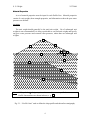
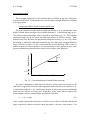
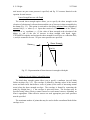
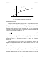
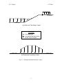
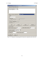
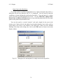
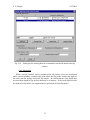
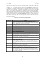
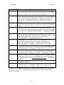
UTEXASED4
A COMPUTER PROGRAM FOR
SLOPE STABILITY CALCULATIONS
(Educational version of the UTEXAS4
and TexGraf4 software)
IMPORTANT NOTICE:
This software and all associated electronic media and documentation are provided for use
by the faculty and students of the licensed university or educational institution for
educational purposes only. The licensed university is designated on the startup screen of
the UTEXASED4 application software. The software may not be used for commercial
purposes or research. The software also may not be distributed to or used by others
outside the university or educational institution to which it is licensed.
Copyright 2004 by Stephen G. Wright – All rights
reserved
March 2004
Austin, Texas
S. G. Wright
2/27/2004
Section 1 - Introduction
UTEXASED4 is the educational version of the UTEXAS4 and TexGraf4 software
for slope stability calculations. The software performs limit equilibrium slope stability
calculations for a factor of safety. Computations can be performed for homogeneous and
inhomogeneous slopes using both circular and noncircular slip (potential sliding)
surfaces. The factor of safety, F, is defined with respect to shear strength as,
F=
Available shear strength
s
=
Shear stress forequilibrium τ
(1.1)
Shear strength may be expressed using either effective stresses or total stresses. For
effective stresses the shear strength is expressed as,
s = c' + (σ - u) tanφ'
(1.2)
where c' and φ' are the cohesion and friction angle, respectively, expressed in terms of
effective stresses. For total stresses the shear strength is expressed as,
s = c + σ tanφ
(1.3)
where c and φ are the cohesion and friction angle, respectively, expressed in terms of
total stresses.
For circular slip surfaces computations can be performed using either Bishop's (1955)
"Simplified" procedure or Spencer's (1967) procedure. For noncircular slip surfaces
Spencer’s (1967) procedure is always used. Several different options including
computations for a single, specified slip surface and searches to locate a minimum factor
of safety are available in UTEXASED4. These options are described as part of the
description of Analysis/Computation Data in Section 4 of this manual.
Coordinate System and Units
Coordinates for the slope geometry, slip surfaces, piezometric line, etc. are specified
using a right-hand Cartesian coordinate system with the x axis being horizontal and
positive to the right and the y axis being vertical and positive in the upward direction.
Coordinate values may be both positive and negative and the slope may face to either the
left or the right.
Any consistent set of length and force units may be used for a problem, e.g. feet,
pounds, pounds per foot, pounds per square foot and pounds per cubic foot. The software
provides for three specific, “standard” sets of units for which the default value for the unit
weight of water and the numbers of decimals places used to output coordinates, strengths,
1
S. G. Wright
2/27/2004
distributed loads, etc. are specially configured. Use of one of the three “standard” sets of
units is recommended. The three standard sets of units are as follows:
1. Feet and pounds.
2. Meters and Newtons (SI units).
3. Meters and Kilonewtons
The type of units is selected using the Units command in the UTEXASED4 Data menu.
Units are described in further detail in Section 4.
2
S. G. Wright
2/27/2004
Section 2 - Description of Problem
Several "Groups" of data are required to describe a problem. The data include the
following:
1.
"Profile Lines", which define the slope profile and subsurface stratigraphy,
2.
Material properties for the soils in the cross-section,
3.
Piezometric line, which are one of the options for defining pore water
pressures,
4.
Distributed, external loads (stresses, pressures) on the surface of the slope.
5.
Internal soil “reinforcement” such as geogrids, soil nails, tie-back anchors
and piles or piers,
6.
"Analysis/Computation" data that describe the type of slip surface (circular
or noncircular) to be used and whether a single slip surface is to be analyzed
or a search is to be conducted to find a “critical” slip surface with a minimum
factor of safety. The Analysis/Computation data also include several other
parameters that affect the computations, including the presence of a “tension
crack”.
Each of the "Groups" of input data is described further in this section.
Profile Lines
Profile Lines define the slope geometry and subsurface stratigraphy (Fig. 2.1). The
soil beneath a Profile Line is assumed to have a given set of material properties until
another Profile Line is encountered at a lower depth. The Profile Lines are defined by the
coordinates of two or more points along the line from left-to-right. Straight lines are
assumed to connect the points. Profile Lines cannot intersect (cross) other Profile Lines;
however, Profile Lines can meet (touch). Profile Lines also cannot coincide over any
portion of their length; if two Profile Lines were to coincide, the underlying soil would
not be uniquely defined.
The slope geometry is automatically determined by UTEXASED4 from the input data
for the Profile Lines. The slope profile is taken as the uppermost surface formed by one,
or possibly several, Profile Lines.
3
S. G. Wright
2/27/2004
Material Properties
A set of material properties must be input for each Profile Line. Material properties
consist of a unit weight, shear strength properties, and information on how the pore water
pressures are defined.
Unit Weight
The unit weight should generally be the total unit weight. Use of submerged unit
weights is not recommended: It is always preferable to use total unit weights and specify
any pore water pressures and external water pressures, rather than use submerged unit
weights.
6
6
6
5
4
5
4
3
2
2
1
Note: Solid symbols ( ) designate points where coordinates are specified.
Profile Line numbers are shown in boxes, e. g. 1
Fig. 2.1 – “Profile Lines” used to define the slope profile and subsurface stratigraphy.
4
S. G. Wright
2/27/2004
Shear Strength Properties
Shear strength properties for each material may be defined in any one of the three
ways described below. Each material may have the shear strength defined in a different
way if appropriate.
Conventional Mohr-Coulomb Cohesion and Friction
Shear Stress, τ
The most common way that shear strengths are defined is by a conventional, linear
Mohr-Coulomb failure envelope with a cohesion intercept (c, c') and friction angle (φ, φ').
The cohesion and friction angle must be entered as input data (Fig. 2.2). The cohesion
and friction angle may be the values for either total stresses or effective stresses. Some
materials may have the shear strength defined using total stresses, e.g. for a clay where
the loading is undrained, while other materials may have their shear strength defined in
terms of effective stresses, e. g. for a coarse sand that is freely draining. If the values are
defined in terms of effective stresses, it is also necessary to enter appropriate pore water
pressure information as described later in the section on pore water pressures.
φ, φ'
c, c'
Total or Effective Normal Stress, σ or σ'
Fig. 2.2 - Conventional Mohr-Coulomb failure envelope.
No special distinction is made between effective stresses and total stresses in the
input data except for the selection of the appropriate numerical values for cohesion (c vs.
c') and friction angle (φ vs. φ'), and the specification of pore water pressure information
when effective stresses are being used. Regardless of the values that are entered, the
shear strength is always computed from an equation of the form:
(2.1)
s = c + (σ - u) tanφ
where c and φ represent the total stress or effective stress values of cohesion and friction
angle, respectively, that are entered as input data and u is the pore water pressure. For
5
S. G. Wright
2/27/2004
total stresses no pore water pressure is specified, and Eq. 2.1 becomes identical to the
equation for total stresses.
Linear Strength Increase with Depth
The second shear strength option allows you to specify the shear strength at the
elevation of a horizontal, reference datum and the rate of increase in shear strength below
the datum (Fig. 2.3). This option is restricted to describing undrained shear strengths of
saturated clays, i. e. where φ = 0. Input data consist of (1) the elevation of the "datum",
expressed as a y coordinate, y o , (2) the value of shear strength at the elevation of the
datum, s o , and (3) the rate of increase in shear strength with depth, ∆s ∆y .
UTEXASED4 computes and assigns the shear strength for each slice as a cohesion value,
c, and φ is assumed to be zero. No pore water pressures are specified.
so
Datum, yo
Shear Strength
Depth
∆s/∆y
Fig. 2.3 - Representation of linear increase in strength with depth.
Nonlinear (Curved) Mohr-Coulomb Envelope
The third shear strength option allows you to specify a nonlinear (curved) Mohr
failure envelope (Fig. 2.4). The envelope is defined by entering values of the normal
stress and shear stress that define a series of points (in the order of increasing normal
stress) along the shear strength envelope. The envelope is formed by connecting the
points by straight lines, i. e. the envelope is piecewise linear. The envelope may be
specified using either effective normal stresses or total normal stresses, depending on
what is appropriate. When effective stresses are used appropriate pore water pressures
must be specified.
The maximum number of points that may be used to define a nonlinear Mohr failure
envelope is six.
6
2/27/2004
Shear Stress, τ
S. G. Wright
Specified
Points
Total or Effective Normal Stress, σ or σ'
Fig. 2.4 - Nonlinear (curved) Mohr failure envelope.
Pore Water Pressure Information
When shear strengths are expressed as a function of effective stresses pore water
pressure information must also be specified. If the shear strength is specified in terms of
total stresses, no pore water pressures are specified (pore water pressures should be
specified as zero). Non-zero pore water pressures may be specified either by a constant
pore water pressure coefficient, ru, or by a piezometric line. The pore water pressure
coefficient, ru, is the ratio between the pore water pressure (u) and the corresponding total
vertical overburden pressure (γz) at any point, i. e.
ru =
u
γz
(2.2)
where γ is the total unit weight of soil and z is the vertical depth below the surface of the
slope to the point where the pore water pressure is defined. When the pore water
pressures are defined by a value of ru , the value of ru is entered with the material
property data.
When a piezometric line is used to define the pore water pressures the actual data
defining the location of the piezometric line are entered separately (See the next section
on Piezometric Line).
Piezometric Line
A piezometric line is one way that pore water pressures may be defined when the
shear strength is expressed using effective stresses. When a piezometric line is used, pore
water pressures are computed by multiplying the vertical distance between the
piezometric line and the center of the base of each slice by the unit weight of water. Pore
7
S. G. Wright
2/27/2004
water pressures are positive below the piezometric line and negative above the
piezometric line.
A piezometric line is defined by specifying the coordinates of a set of points along the
piezometric line from left to right. Straight lines are assumed to connect the points to
define the piezometric line.
The single piezometric line may be used to define pore water pressures in more than
one material.
Distributed Loads
Distributed load data are used to represent pressures acting on the surface of the
slope. Distributed loads are used to represent the water on or adjacent to the slope as well
as loads due to footings or similar structural loads (Fig. 2.5). Because a two-dimensional
planar cross-section is analyzed, distributed loads represent strip loads that extend to
infinity in the direction perpendicular to the plane of the two-dimensional cross-section.
Distributed loads are entered by specifying a series of points along the surface of the
slope. At each point the x-y coordinates of the point and the corresponding value of
pressure (normal stress) are specified. Pressures are assumed to vary linearly between
points and are zero to the left of the first point and to the right of the last point. If the
distributed load abruptly changes, i. e. a “step” load exists, the point where the load
changes is entered twice - once with the value of the pressure to the left of the point and,
the second time, with the value of the pressure to the right of the point.
Reinforcement Lines
Reinforcement lines are used to describe internal soil reinforcement. Each line of
reinforcement is defined by a series of points along the length of the reinforcement and
the value of longitudinal (axial) and transverse (shear) force at each point.
Reinforcement may be vertical, horizontal or inclined (Fig. 2.6).
Longitudinal reinforcement forces that are tensile are considered to be positive;
compressive reinforcement forces are negative. The sign convention for shear forces is
shown in Fig. 2.7.
8
S. G. Wright
2/27/2004
(a) Water and "Surcharge" Loads
LEGEND
- Load specified
- Load specified twice (once
for left, once for right)
(b) Distributed Foundation Loads
Fig. 2.5 – Example distributed loads on “slope”.
9
S. G. Wright
2/27/2004
LEGEND
Reinforcing line
Specified points
(a) Slope reinforced with Geosynthetics
(b) Anchored (tie-back) wall
(c) Pile-reinforced slope
Fig. 2.6 – Example reinforcement “lines” in slopes.
10
S. G. Wright
2/27/2004
Fig. 2.7 – Sign convention for shear forces in reinforcement.
11
S. G. Wright
2/27/2004
Analysis/Computation Data
The Analysis/Computation data define the type of computations to be performed.
This includes the shape of the slip surface and information pertaining to whether a single
slip surface is to be analyzed or an automatic search is to be conducted to locate a
"critical" slip surface with the lowest factor of safety. Four different types of
computations can be performed as described below.
Automatic Search with Circular Slip Surfaces
An automatic search can be performed to locate a “critical” circle that produces a
minimum factor of safety. For the search the location of the center point and radius of
circles are systematically varied until a minimum factor of safety is found. Care must be
exercised because the factor of safety found by an automatic search may only represent a
“local” minimum. It may be necessary to initiate searches with several different starting
conditions (center point and radius) to be sure that the overall minimum factor of safety is
found.
For the automatic search you must enter a starting point for the center of the circle
and the initial elevation for the bottom of trial circles. The center point and depth of
circles will be varied from the starting point to find the most critical circle. A maximum
depth, expressed as limiting elevation, y, is also specified. Circles are not allowed to pass
below the limiting depth.
The automatic search is conducted by first finding the most critical circle passing to
the starting depth (y elevation) indicated. The centers of circles are varied using a 9-point
(3 x 3) grid, which is moved repeatedly. The grid is moved until the circle with its center
at the center of the grid has the lowest factor of safety relative to the circles with centers
at the eight points on the perimeter of the grid. Also, as the grid is moved, the size of the
grid is varied until the final, smallest spacing between adjacent center points is 2.5
percent (0.025) of the slope height. The initial grid spacing is chosen to be 40 times the
final spacing, i. e. the initial grid spacing is equal to the slope height.
Interactive, “Manual” Search with Circular Slip Surfaces
Instead of having the search performed automatically, UTEXASED allows you to
conduct the search manually by selecting each trial center point by clicking in the main
display window with the mouse. For each center point selected the radius of the circle is
varied to find the radius producing the lowest factor of safety. Radii are varied
automatically between maximum and minimum values designated by the user as part of
the input data. The increment used to vary the radii between the maximum and minimum
values is also designated by input data.
12
S. G. Wright
2/27/2004
Once at least three center points have been entered and the factor of safety
successfully computed for each center point contours of factor of safety are drawn. The
contours are based on the lowest factor of safety calculated for each center point. The
contours can be used to judge where the next center point should be located and in this
way a "search" can be conducted to find a minimum. This search can also be used to find
multiple, local minimums if they exist.
Individual Noncircular Shear Surface
The third analysis option allows you to perform computations for a single, selected
noncircular slip surface. The Analysis/Computation data consist of the coordinates of
points along the selected slip surface from left to right. Straight lines are assumed to
connect the points to form a continuous, piecewise linear surface. The first and last
points on the slip surface must be located on the surface of the slope.
Automatic Search with Noncircular Slip Surfaces
The fourth and final analysis option allows an automatic search to be conducted to
find a noncircular slip surface with a minimum factor of safety. The search is conducted
using a procedure similar to the one developed by Celestino and Duncan (1981). The
search is started with an initial, assumed trial slip surface, which is defined by the
coordinates of a set of points along the slip surface from left to right. Each point on the
initial slip surface is then moved some distance in two directions, e.g. up and down, and
the factor of safety is computed for each of the two moves. After all points on the initial
trial slip surface have been moved, the location of the slip surface is adjusted and the
process is repeated. The amount each point is moved is reduced as the search progresses.
The direction that each point is moved and the initial and final distances that points are
moved are entered as part of the input data for the search.
"Tension" Crack
The depth of a vertical "tension" crack and the depth of water in the crack may also
be entered as part of the input data for either circular or noncircular slip surfaces. When a
tension crack is specified, UTEXASED4 automatically terminates the slip surface at a
depth corresponding to the bottom of the crack, near the upslope end of the slip surface.
Limitations on Problem Size
The educational version of the UTEXAS4 software limits the size of the problem you
can run by limiting the number of Profile Lines, piezometric lines and reinforcement lines
that can be entered. The number of points that can be entered on any one line as well as
to define noncircular slip surfaces is also limited. To determine the current limitations
for the version of UTEXASED4 that you are using, start the program and choose the
13
S. G. Wright
2/27/2004
Limitations command from the Data menu. A Dialog box like the one shown in Fig. 2.8
is then displayed showing the limitations.
Fig. 2.8 – Dialog box used to display limitations on problem data size for UTEXASED4.
14
S. G. Wright
2/27/2004
Section 3 - Preparing Your Data
Prior to running UTEXASED4 you should prepare the data for your problem for
input. Make a scale drawing of the slope and determine the coordinates of points
defining each of the Profile Lines that you will be using. Also determine what unit
weight and shear strength properties will be assigned to each material. If shear strengths
are expressed using effective stresses, determine how the pore water pressures will be
defined for each material. If a piezometric line will be used to define pore water
pressures, determine the coordinates of the points that will be used to define the
piezometric line.
If there are external, distributed loads on the slope, determine the appropriate
locations of the points that will be used to define the loads. In general points will need to
be defined where the load starts and ends as well as where the rate of change in
distributed load changes significantly.
If the slope has reinforcement, e. g geogrids, piers or tie-back anchors, you need to
determine the coordinates of points that define each line of reinforcement and the values
of longitudinal (axial) and transverse (shear) force at each point. UTEXASED4 limits the
number of points that you can use to define each reinforcement line to four.
You will also need to decide whether to perform computations using circular or
noncircular slip surfaces. For an automatic search with circles you will need to select a
reasonable center point for starting the search as well as an initial depth (y elevation) for
the bottom of the circles. For an interactive, manual “search” with circles the radii will
be varied for each trial center point. You will need to determine the minimum and
maximum radii to be used. For computations with noncircular slip surfaces determine the
coordinates of points along either the single noncircular slip surface to be analyzed or, in
the case of a search, the initial trial noncircular slip surface.
15
S. G. Wright
2/27/2004
Section 4 - Entering and Checking Input Data
To run UTEXASED4 follow the instructions you should have been given for starting
UTEXASED4 on the computer system you are using. Once UTEXASED4 is running you
should see the main display window with a menu bar at the top. You are then ready to
begin entering your input data.
Data are entered into UTEXASED4 using commands in the Data menu and dialog
boxes. At any time while you are entering data, you can save the data using the Save
command in the File menu. Entry of each group of data is described in the section
below. In general you should enter data in the order they are described below, but once
data are entered you can always go back and correct or modify your input in any
sequence.
When you enter data such as Profile Lines that can be represented graphically the data
are displayed in the main display window of UTEXASED4. As each group of data
(Profile Lines, piezometric line, slip surface, etc.) is entered, it is displayed in the main
window. However, the display is not immediately updated as the data are entered and
changed in a dialog box. You must first dismiss the dialog box by clicking on the OK
button before the display reflects the changes.
Units
Before entering input data for the problem, you should select the type of units you
will be using. Choose the Units command from the Settings menu. A dialog box like
the one shown in Fig. 4.1 then appears. Use the dropdown list labeled “Type of Units”
to select one of the following:
•
Feet and Pounds
•
SI – Meters and Newtons
•
Meters and Kilonewtons
Depending on the type of units selected the units that will be assumed for length, force,
stress, etc. will be shown in the lower part of the dialog box. The default value for the
unit weight of water (or other fluid) is also shown.
The default value for the unit weight of water is assigned to data provided that
you have not specifically entered a value for the unit weight of water separately. The unit
weight of water is entered by choosing the Unit Weight of Water command from the
Data menu. Once you enter a value for the unit weight of water, the default value for the
16
S. G. Wright
2/27/2004
unit weight of water is no longer used. The default value is only used when you first start
UTEXASED4. Also, once you have entered a value for the unit weight of water,
changing the type of units using the Units item in the Data menu will not reset the
default value for the unit weight of water. However, if you change the units using the
Units command, the change will affect the numbers of decimals that are used to display
data.
Fig. 4.1 – Dialog box for selecting type of units for problem.
Profile Lines
To enter data for the Profile Lines choose the Profile Lines command from the Data
menu. When you do, a dialog box like the one shown in Fig. 4.2 is displayed for you to
start entering data. The tabs at the top of the dialog box are used to select individual
Profile Lines for data entry. The numbering of lines and order of data entry for lines does
not matter. You may enter data in any order and for any line numbers. Only lines for
which coordinates of two or more points have been entered are used. To enter data for a
particular line, first select the line number by clicking on the appropriate tab at the top of
the dialog box. Enter x-y coordinates of points along the line by typing them in the boxes
provided at the bottom of the dialog box (x-value is in first box, y-value is in second
box). Click on the Add Point button to accept the values you have typed; the values
should then appear in the list in the upper portion of the dialog box. Repeat this for
additional points along the Profile Line by typing x-y values and then clicking on the
Add Point button. You can also enter values by typing them in the boxes and pressing
the Enter key on the keyboard, provided that the edit text boxes for entering the x and y
values have the current focus for input. Points that you enter will automatically be sorted
so that they are in a left-to-right order. If two points have the same x value, i. e. a
segment of a Profile Line is vertical, you will be prompted when you enter the second
such point. In this case a dialog box is displayed for you to select whether you want the
17
S. G. Wright
2/27/2004
point inserted before or after the other point with the same x value. After you have
chosen whether the point is to be before or after the other point, the point is added to the
list in the appropriate place.
Fig. 4.2 - Dialog box for entering Profile Line data.
As soon as you enter a point the Change Point, Delete Point and Delete All buttons
at the bottom of the dialog box become active. Use the Change Point button to change
the coordinate of a point that you have already entered. To change the values, first select
the point by clicking on its coordinates in the list box. The coordinates then appear in the
text boxes at the bottom of the dialog box. You can then enter new values by changing
the values in the text boxes. When you have changed the values to what you want, click
on the Change Point button to accept the changes. The new values then appear in the list
box. If the new values change the order of the points, the new values will be displayed at
the appropriate place in the list. Also if the new x value is the same as the x value for
another point, you will be prompted to choose whether the point you have edited is to go
before or after the other point with the same x value.
The Delete Point button is used to remove an unwanted point that you have entered.
To remove a point first select its coordinates in the list box. Then, click on the Delete
Point button to remove the point.
18
S. G. Wright
2/27/2004
The Delete All button is used to delete all of the points for the current Profile Line.
The Delete All button only deletes the points for the current line; data for other lines are
not affected.
To enter another Profile Line, click on the appropriate tab at the top of the dialog box
and enter data in the same way that you entered data for the first line. Repeat this process
until data for all lines have been entered. Profile lines may be entered and numbered in
any order. In fact numbers do not need to be in continuous sequence, e.g. Profile Lines 1,
2, and 4 may be entered, while Profile Line number 3 is omitted.
When finished entering the Profile Line data, click on the OK button. Clicking on
the Cancel button will cause any data that you have entered or changed to be ignored.
Once you have entered the Profile Line data it is a good idea to save your data before
proceeding to enter data for the material properties. Use the Save command in the Data
menu to save your data. You can return to the Profile Line dialog box at any time later.
When you do, the data, which you have entered will be displayed in the dialog box.
Material Properties
To enter material properties choose the Material Properties command from the Data
menu. A dialog box similar to the one shown in Fig. 4.3 is displayed for you to enter
data. Tabs at the top of the dialog box correspond to the materials for each Profile Line
that was entered. If you have not entered any Profile Line data, when you choose the
Material Properties command from the Data menu, a warning message is displayed
instead of the dialog box. You must enter Profile Line data before you can enter material
properties.
Enter the data for material properties in the dialog box. Option lists are shown for
both the shear strength and pore water pressures. The available required data and options
are described below.
Unit Weight
Enter the total unit weight in the text box provided for each material.
Shear Strength Data
Three options are available in the Shear Strength Option list: (1) "Conventional:
cohesion, friction angle", (2) "Linear increase in undrained strength below horiz. datum",
and (3) "Nonlinear (curved) Mohr failure envelope". To select a strength option click on
the dropdown list labeled "Shear strength option:". A list of the available strength
options will appear for you to choose an option. Depending on the option you choose,
the dialog box and information entered will change. If you choose "Conventional:
cohesion, friction Angle", the area for entering shear strength properties should look like
19
S. G. Wright
2/27/2004
the one shown in Fig. 4.3. If you choose "Linear increase in undrained strength below
horiz. datum", the area for entering strength properties in the dialog box will change to
look like the one shown in Fig. 4.4. You will then enter the elevation (y) of the
horizontal datum, the value of the shear strength at the datum elevation and the rate of
strength increase below the datum.
Fig. 4.3 - Dialog box for entering material properties.
If you choose "Nonlinear (curved) Mohr failure envelope" as the strength option, the
area of the dialog box for entering shear strength properties will look similar to the one
shown in Fig. 4.5. To enter data for a nonlinear Mohr failure envelope type values for the
normal stress and shear stress in the text boxes at the bottom of the list box where the
nonlinear envelope is displayed. Click on the Add Point button once you have typed in
the values of normal and shear stress to add the point to the list of points for the nonlinear
20
S. G. Wright
2/27/2004
envelope. Once you have clicked on the Add Point button, the values appear in the list
box. Points must be arranged in the order of increasing normal stress and no two points
may have the same value of normal stress. Points are automatically inserted in the list in
the proper order when you enter them; the actual order you enter values does not matter.
Fig. 4.4 - Dialog box for entering material properties when the undrained shear strength
increases linearly with depth.
The maximum number of points that can be entered to define a nonlinear Mohr
failure envelope is six.
To change the value of normal or shear stress for a point, first select the point by
clicking on the values that define the point in the list box. The values of normal and
21
S. G. Wright
2/27/2004
shear stress will appear in the text boxes at the bottom of the list box. Change the values
by typing in new values in the text boxes. Once you have changed the values as desired,
click on the Change Point button to update the values in the list box. The new values
then appear in the list of values. If the new values change the order of the points the
points will be re-ordered in the proper sequence of increasing normal stress values. Note
that no changes are saved unless you click on the Change Point button.
To delete a point that you have already entered for the nonlinear envelope, first
select the point by clicking on the appropriate values of normal stress and shear stress in
the list box. Then, click on the Delete Point button to delete the selected point. To
delete all of the points on the nonlinear envelope click on the Delete All Points button.
Fig. 4.5 - Dialog box for entering material properties when a nonlinear (curved) Mohr
failure envelope is used
22
S. G. Wright
2/27/2004
Pore Water Pressures
A dropdown list labeled “Pore water pressure option” is used to select how the pore
water pressures are defined for each material. The list presents three options: (1) "No
pore pressure (or total stresses)", (2) "Constant pore pressure coefficient (r-sub-u)", and
(3) "Piezometric line". To select a pore water pressure option click on the dropdown list
labeled "Pore water pressure option:". The list of three available pore water pressure
options is then displayed for you to select an option. Depending on the option you
choose the dialog box and information entered will change. If you choose "No Pore
Pressure (or Total Stresses)", no additional information is required to define the pore
water pressures. If you choose "Constant pore pressure coefficient (r-sub-u)" as the
option, the area for entering pore water pressures in the dialog box will change to look
like the one shown in Fig. 4.3. You should then type the value of the pore water pressure
coefficient, ru , in the text box provided. If you choose "Piezometric line" as the pore
water pressure option, the area for entering the pore water pressure information will look
like the one illustrated in Fig. 4.5.
Unit Weight of Water
The unit weight of water is used to compute pore water pressures from a piezometric
line and to compute the force due to water in an assumed "tension" crack. To enter a unit
weight for water, choose Unit Weight of Water from the Data menu. When you do a
dialog box like the one shown in Fig. 4.6 is displayed. Type a value in the text box
provided and press the OK button to change the unit weight of water.
Fig. 4.6 - Dialog box for entering the unit weight of water.
Initially a default value is assumed for the unit weight of water. The default value is
determined according to the type of units, which is set using the Units command in the
Settings menu. However, once you enter a unit weight of water using the Unit Weight
of Water menu item and the dialog box shown in Fig. 4.6, the default value is no longer
applicable. Even if you change the type of units, the unit weight of water will remain the
value set using the Unit Weight of Water menu item.
23
S. G. Wright
2/27/2004
Piezometric Line
To enter data for the piezometric line choose the Piezometric Line command from
the Data menu. A dialog box similar to the one shown in Fig. 4.7 is then displayed. If
none of the materials entered use a piezometric line to define pore water pressures, a
warning message instead of the dialog box is displayed when you choose the
Piezometric Line command. You can only enter data for a piezometric line when the
piezometric line has been used to define pore water pressures for at least one material.
Thus, material properties must always be entered before entering piezometric line data.
Data for the piezometric line are entered in almost the same way that you enter data
for Profile Lines. Values are entered by typing them in the text boxes provided and
clicking on the Add Point button. Use the Change Point, Delete Point and Delete All
buttons to change and delete points as described earlier for the Profile Lines.
Fig. 4.7 - Dialog box for entering data for the Piezometric Line.
24
S. G. Wright
2/27/2004
Distributed Load Data
To enter data for distributed loads (pressures) on the surface of the slope choose the
Distributed Loads command from the Data menu. A dialog box like the one shown in
Fig. 4.8 is then displayed for you to enter data. Enter the x-y coordinates of the point and
the value of pressure (normal stress) for each point where the distributed load is to be
defined. Click on the Add Point button to accept the values you have typed; the values
will then appear in the list box in the upper portion of the dialog box. Repeat this for
additional points where the distributed load is to be defined by typing x-y-pressure values
and then clicking on the Add Point button. You can also enter values by typing them in
the text boxes and pressing the Enter key on the keyboard. Points that you enter will
automatically be sorted so that they are in a left-to-right order. If two points have the
same x value, i. e. there is a “step” change in distributed load, you will be prompted when
you enter the second such point by a dialog box to select whether you want the point
inserted before or after the other point with the same x value. After choosing whether the
point is to be before or after the other point, the point will be added to the list in the
appropriate place. Use the Change Point, Delete Point and Delete All buttons to change
and delete values as described earlier for Profile Lines.
Fig. 4.8 – Dialog box for entering data for distributed loads
25
S. G. Wright
2/27/2004
Reinforcement Data
To enter data for internal reinforcing lines choose the Reinforcement Lines
command from the Data menu. A dialog box like the one shown in Fig. 4.9 is then
displayed for you to enter data. The tabs at the top of the dialog box are used to select
individual reinforcement lines for data entry. The numbering of lines and order of data
entry for lines does not matter. You may enter data for lines in any order and for any line
numbers. Only lines for which data have been entered are used.
To enter data for a particular line, first select the line number by clicking on the
appropriate tab at the top of the dialog box. Enter x-y coordinates of points along the line
and the corresponding values of the longitudinal and transverse force by typing them in
the text boxes provided at the bottom of the dialog box. Click on the Add Point button
to accept the values you have typed; the values should appear in the list in the upper
portion of the dialog box. Repeat this for additional points along the reinforcement line
by typing x-y and force values and then clicking on the Add Point button. You can also
enter values by typing them in the boxes and pressing the Enter key on the keyboard.
Use the Change Point, Delete Point and Delete All buttons to change and delete points
on the reinforcement lines as described earlier for Profile Lines.
Fig. 4.9 – Dialog box for entering data for reinforcement lines
26
S. G. Wright
2/27/2004
Analysis/Computation Data
Enter "Analysis/Computation" data by choosing the Analysis Computation
command from the Data menu. A dialog box like the one shown in Fig. 4.10 is then
displayed for you to select the type of analysis. You can select from four choices:
•
An automatic search can be performed using circular slip surfaces to locate a
“critical” circle with a minimum factor of safety.
•
An interactive search, where each trial circle is selected manually, can be
performed.
•
An single, selected noncircular slip surface can be analyzed.
•
An automatic search can be performed to locate a “critical” noncircular slip
surface with a minimum factor of safety.
Choose one of the four options by clicking on the appropriate radio button and then click
on the OK button to dismiss the dialog box. A second dialog box is then displayed for
you to enter the additional data needed for the type of analysis you have chosen. Each
analysis option and the data required are described further below.
Fig. 4.10 – Dialog box for selecting type of analysis to be performed.
27
S. G. Wright
2/27/2004
Automatic Search with Circles
If you choose to perform an automatic search with circular slip surfaces a dialog box
like the one shown in Fig. 4.11 is displayed. Enter the x-y coordinates of the center point
where the automatic search is to start as well as the elevation of the bottom of the initial
trial circle. Also enter a maximum depth allowed for circles; the maximum depth is
expressed as an elevation (y) of the bottom of circles. Type each of these values in the
appropriate text boxes shown in Fig. 4.11.
For circles you can choose either the Simplified Bishop or Spencer's procedure for the
analysis. Use the dropdown list labeled Procedure of analysis to choose the procedure
to be used.
You can also specify a vertical “tension” crack and a depth (height) for the water in
the tension crack. Enter values for the depth of crack and the depth of water in the crack
by typing them in the boxes at the bottom of the dialog box. When you have finished
entering all the data in the dialog box, click on the OK button to return to the main
display window.
Fig. 4.11 – Dialog box for entering data for an automatic search with circles
28
S. G. Wright
2/27/2004
Interactive (Manual) “Search” with Circles
If you choose an interactive search with circles a dialog box like the one shown in
Fig. 4.12 is displayed. This dialog box is used to enter information needed for the
interactive search. The upper approximately two-thirds of the dialog box is used to enter
information that defines the range of radii that will be tried for each trial center point, i. e.
the information defines the maximum and minimum radii that will be tried. The radii
may be defined by (1) a value of radius, (2) a point through which the circles pass, or (3)
a line to which the circles are tangent. Use the "dropdown" list labeled "Maximum or
minimum radius defined by" to choose how the radius is defined. Then enter the
appropriate data needed for each criterion (radius definition) in the text boxes located
below the dropdown list. For example, if the radius is defined by a specific value of
radius, enter the radius. Once a criterion has been chosen for defining the radii and the
required data have been entered, click on the Add button to add the criterion. The
criterion then appears in the list box. A minimum of two criteria must be selected and
entered to define the range of trial radii for each center point. You may enter any number
of criteria in excess of two to specify the range of radii to be used. Regardless of the
number of criteria entered the range for radii is determined for each center point by the
maximum and minimum radius that results from the chosen criteria and current center
point coordinates. If more than two criteria are chosen, different pairs of criteria may
govern the maximum and minimum radius depending on the particular location of the
center point.
Radii are varied beginning with a coarse increment and then reducing the size of the
increment. The initial increment is determined by dividing the difference between the
maximum and minimum radius by a number. This number is entered as the "Number of
radius increments" in the dialog box shown in Fig. 4.12. Radii are varied in
successively smaller increments until a minimum value of the increment is reached. The
minimum value of the radius increment is entered as the "Minimum radius increment"
in the dialog box shown in Fig. 4.12.
The procedure of analysis (Simplified Bishop or Spencer) is chosen using the
dropdown list in the dialog box labeled Procedure of analysis.
The depth of a vertical crack and the depth of any water in the crack are the final
(optional) data that are entered in the dialog box shown in Fig. 4.12. After entering all
the necessary data in the dialog box, click on the OK button to continue.
29
S. G. Wright
2/27/2004
Fig. 4.12 – Dialog box for entering data for interactive (manual) search with circles
30
S. G. Wright
2/27/2004
Single Noncircular Slip Surface
If you have chose to perform computations for a single noncircular slip surface, a
dialog box like the one shown in Fig. 4.13 is displayed. You will need to enter the
coordinates of points defining the noncircular slip surface. Type each pair of x-y values
in the text boxes provided beneath the list box. Use the Add Point, Change Point,
Delete Point and Delete All Points buttons to enter and edit points much like you enter
points on the profile and piezometric lines.
You can also specify a vertical “tension” crack and a depth for the water in the
tension crack. Enter values for the depth of crack and the depth of water in the crack by
typing them in the boxes at the bottom of the dialog box. When you have finished
entering all the data in the dialog box, click on the OK button to return to the main
display window.
Fig. 4.13 – Dialog box for entering data for a single noncircular slip surface.
31
S. G. Wright
2/27/2004
Automatic Search with Noncircular Slip Surfaces
If you chose to perform an automatic search with noncircular slip surfaces, a dialog
box like the one shown in Fig. 4.14 is displayed. You will need to enter the coordinates
of points that define the initial trial noncircular slip surface. Also, for each point you
must designate whether the point is to be fixed during the search or moveable, and if
moveable, the direction for shifting the point. Coordinates of points are entered by typing
the values in the text boxes labeled X and Y. Information for shifting each point is
entered using the drop-down list to the right of where the coordinates are entered. Click
on the drop-down list to choose how the point is to be shifted from one of the following
four options:
•
Point is shifted approximately perpendicular to the slip surface.
•
Point is shifted horizontally
•
Point is shifted vertically
•
Point is fixed – not shifted
Shifting of the two end points of the slip surface is constrained to the slope and any
direction that you enter for the end points (except fixed) is ignored. Once you have
entered the coordinates in the text boxes and chosen how the point is to be shifted, click
on the Add Point button to add the point to the list of points already entered. Use the
Change Point, Delete Point and Delete All Points buttons to edit points much like you
edit points on profile and piezometric lines.
You must also enter an initial and final distance for shifting points on the noncircular
slip surface during the automatic search. The search will begin by shifting points by the
“Initial distance” that you specify. The distance will then be progressively reduced as the
search proceeds until the distance is less than the “Final distance” specified, at which
point the search is stopped. Enter the distances for shifting points in the boxes labeled
Initial distance for shifting points and Final distance for shifting points.
You can also specify a vertical “tension” crack and a depth for the water in the
tension crack. Enter values for the depth of crack and the depth of water by typing them
in the boxes at the bottom of the dialog box. When you have finished entering all the data
in the dialog box, click on the OK button to return to the main display window.
32
S. G. Wright
2/27/2004
Fig. 4.14 – Dialog box for entering data for an automatic search with noncircular slip
surfaces.
Crack Information
When a vertical "tension" crack is introduced the slip surface (slices) are terminated
and a vertical boundary is added at the point where the slip surface reaches the depth of
the crack, near the upslope end of the slip surface. Be careful that the crack depth does
not exceed the depth of slip surfaces that may be of interest. If the crack depth exceeds
the depth of a slip surface, no computations are performed for that slip surface.
33
S. G. Wright
2/27/2004
Checking Input Data
Once you have created your input data the data should be checked before attempting
to run UTEXASED4. To check the data choose the Check Data command from the
Data menu.
If errors are detected in your input data when the Check Data command is chosen, a
dialog box similar to the one shown in Fig. 4.15 is displayed. This dialog box can be
used to view all of the errors detected. Click on the Next Error button to advance to the
next error. Similarly use the First Error, Previous Error and Last Error buttons to
move to the first, previous and last errors, respectively. Some buttons may be dimmed
when you are at either the start or end of the errors list: The First Error and Previous
Error buttons are dimmed when the first error is displayed; the Next Error and Last
Error buttons are dimmed when the last error is displayed.
Fig. 4.15 - Dialog box used to display error messages
If your input data contain errors, correct them before proceeding with the
computations. Errors displayed in the dialog box are not automatically removed from the
dialog box when you correct your data. The errors displayed are only removed from the
dialog box and updated when you check your data again. To re-check your data and
confirm your corrections, choose the Check Data command again. If there are still
errors, the dialog box will be updated to show any errors that still exist.
34
S. G. Wright
2/27/2004
Section 5 - Performing the Computations
After you have created your input data and corrected any errors you are ready to
perform the stability computations. To start the computations choose Do Computations
from the Computations menu. Depending on the type of computations you chose the
response will differ as described further below:
Automatic Search with Circles
If you chose to perform an automatic search with circular slip surfaces, the various
trial circles and factors of safety are displayed as the computations are performed.
However, before the computations begin a dialog box like the one shown in Fig. 4.16 is
displayed for you to enter additional information related to what is displayed as follows:
Search Delay: The search delay area allows you to choose a delay between
computation of the factor of safety for each trial circle. With faster computers the
computations may be performed so rapidly that it is difficult to see the sequence
of circles tried. By choosing a delay, you can slow down the computations and
display to make it easier to follow the search.
Circles to Save: Once computations have been completed and the results are
displayed, you can choose how many trial circles will again be displayed.
UTEXASED4 allows you to save a selected number of circles, e.g. ten, to be
displayed with the final results. Use the radio buttons on the right-hand side of
the dialog box to choose an appropriate number of circles to be saved.
After you have made appropriate selections in the dialog box, click on the OK button to
dismiss the dialog box and the computations will begin. Each trial circle is drawn in the
main display window and the corresponding factor of safety for each circle is displayed
in the next to last panel of the Status Bar at the bottom of the display window. The last
panel in the Status Bar displays the lowest value calculated for the factor of safety to that
point. Trial circles are displayed in gray; while the circle having the lowest factor of
safety is displayed in red.
35
S. G. Wright
2/27/2004
Fig. 4.16 - Dialog box for selecting delays between successive trial circles and number of
circles to save for an automatic search with circular slip surfaces.
Once the automatic search is completed, you can display the most critical circle,
including the individual slices and the distribution of stresses along the circle by clicking
once in the main display window. This will cause the display to change from showing all
the trial circles to showing the critical circle. Also, if you indicated that some trial circles
were to be saved (See Fig. 4.16), the circles that were saved are also displayed.
Interactive (Manual) “Search” with Circles
If you chose to perform an interactive “search”, the dialog box shown in Fig. 4.17 is
displayed. During the interactive search the main display window and a separate “Graph
Window” are displayed. The Graph Window shows how the factor of safety varies with
the radius of the circle for the most recent center point entered. The dialog box shown in
Fig. 4.17 is displayed to allow you to choose to have the windows arranged automatically
so that they do not overlap (you can later rearrange the windows differently if you wish).
It is generally recommended that you allow the windows to be arraigned automatically by
clicking on the Yes button. Choose No if you do not want the windows automatically
arranged; choose Cancel if you do not want the interactive search to start.
Fig. 4.17 – Dialog box displayed at start of interactive search.
If you clicked on the Yes or No button, you are now ready to start the interactive
search. Begin by selecting a center point for a trial circle by clicking in the main display
window at the location of the center point. If the computations are successful the trial
36
S. G. Wright
2/27/2004
circles are displayed in the main display window and the variation in factor of safety with
radius is displayed in the “Graph Window”. Also as each trial circle (radius) is attempted
the factor of safety is displayed in the Status Bar at the bottom of the main display
window in the box labeled "F". The lowest factor of safety calculated for the trial center
point is also displayed on the far right in the Status Bar in the box labeled "F-min".
If the factor of safety can be successfully computed, the center point is displayed as a
gray dot ( ). The center point that produced the lowest factor of safety at any stage in the
"search" also has a small square and "X" displayed at the location, similar to what is
shown below:
If the factor of safety cannot be computed for a center point using any radius, the trial
center point is displayed with a red "X" as follows:
Continue to enter trial center points until you are satisfied that you have located the most
critical circle. Use the contours and the marked location of the most critical center point
to guide your search.
You can halt the search at any time and display the circle that currently has the
minimum factor of safety. To do so, choose the Suspend Interactive Search command
from the Computations menu. The display then changes to show the most critical circle
found to that point along with the individual slices and the distribution of stresses along
the circle. The factor of safety is also shown as text in the area above the slope.
To resume the interactive search once it has been suspended, choose the Resume
Interactive Search command from the Computations menu. The contours of factor of
safety are again displayed and you can continue to select center points for trial circles by
clicking in the main display window.
When you have completed selecting center points for the interactive search choose
the Finish Interactive Search command from the Computations menu. This will end
the search and write the final output tables to the text output file. The Finish Interactive
Search command is identical to the Suspend Interactive Search command except it
completes writing the final information to the text output file and the search cannot be
resumed using the Resume Interactive Search command.
37
S. G. Wright
2/27/2004
Individual Noncircular Slip Surface
If you chose to analyze an individual noncircular slip surface, the computations are
immediately performed and the slip surface is displayed along with the individual slices
and the distribution of effective normal stress and pore water pressure along the slip
surface.
Automatic Search with Noncircular Shear Surfaces
If you chose to perform an automatic search with noncircular slip surfaces, as soon as
you choose the Do Computations command, a dialog box like the one shown in Fig.
4.18 is displayed for you to enter additional information related to what is displayed as
follows:
Search Delay: The search delay area allows you to choose a delay between
computation of the factor of safety for successive shifts of points on the
noncircular slip surface. With faster computers the computations may be
performed so rapidly that it is difficult to see the sequence of shifts. By choosing
a delay, you can slow down the computations and display to make it easier to
follow the search.
Number of Slip Surfaces to Save: Once computations have been completed and
the results are displayed, you can choose how many of the trial noncircular slip
surfaces will be displayed. UTEXASED4 allows you to save a selected number
of slip surfaces, e.g. ten, to be displayed with the final results. Use the radio
buttons on the right-hand side of the dialog box to choose the number of
noncircular slip surfaces to be saved.
After you have made appropriate selections in the dialog box, click on the OK button
and the computations will begin. The shifted position of individual points on the slip
surface will be drawn along with the current position of the most critical slip surface.
The factor of safety for each trial shift is displayed in the next to last panel of the Status
Bar at the bottom of the display window. The last panel in the Status Bar displays the
lowest value calculated for the factor of safety at the current stage of the computations.
The slip surface geometry resulting from each trial shift is displayed in light gray, while
the position of the slip surface with the lowest factor of safety is shown in red.
38
S. G. Wright
2/27/2004
Fig. 4.18 - Dialog box for selecting delays between successive shifts of
points and the number of slip surfaces to save for an
automatic search using noncircular slip surfaces.
39
S. G. Wright
2/27/2004
Section 5 - Graphical Display
Input data, including the Profile Lines, piezometric line and circular and noncircular
slip surfaces that are entered as input data are displayed in the main display window.
Also, once the computations are completed, additional information is displayed. The
display of both the input data and the results of the computations are described separately
below.
Input Data
The input data and colors used for display are summarized in Table 5.1. In addition
to the items listed in Table 5.1 the numbers assigned to the Profile Lines are displayed on
the lines surrounded by a rectangular frame. The slope line may coincide with one or
more Profile Lines and may actually obscure the Profile Line(s) when displayed. All
information pertaining to the input data is displayed before any computations are
performed as well as after computations are completed.
Table 5.1 - Input data displayed and colors used
Item
Color
Profile Lines (numbers shown in rectangles)
Slope Line (may obscure upper-most Profile Line or Lines)
Dark green
Brown w/ surface
hatching
Piezometric Line
Blue
Distributed Loads
Navy (dark) blue
Reinforcement Lines
Magenta
Initial Trial /or/ Designated Slip Surface (Circular or
Noncircular)
Gray
Distributed Load Scaling
Distributed loads are displayed as a series of vectors representing the direction and
magnitude of the distributed stress. The loads (stresses) are scaled based on the current
type of units. Loads are scaled such that the length of the vectors representing the stress
at each point corresponds approximately to an equivalent height of water. This is
particularly useful for checking the validity of data when the distributed loads are
produced by water adjacent to the slope. The scale factors expressed as pressure per unit
distance are shown in Table 5.2.
40
S. G. Wright
2/27/2004
Table 5.2 - Scale factors for distributed loads
Units
Feet and pounds.
Scale Factor
62.4 pounds/square foot/ foot
SI - Meters and newtons.
9800 newtons/square meter/meter
9800 pascals/meter
Meters and kilonewtons.
9.8 kilonewtons/square meter/meter
9.8 kilopascals/meter
Reinforcement Force Scaling
Longitudinal and transverse forces in the reinforcement are represented by a shaded
trapezoidal area representing the magnitude of the force. The forces are scaled based on
the current type of units. The forces are scaled such that the distance representing the
maximum force in the reinforcement is a prescribed length. The lengths representing the
maximum force in the reinforcement are shown in Table 5.3. These lengths are actual
length on the display (computer screen or printed page).
Table 5.3 - Lengths used to represent maximum reinforcement force
Units
Maximum Length
Feet and pounds.
0.5 inch
SI - Meters and newtons.
1 centimeter
Meters and kilonewtons.
1 centimeter
Display During Computations
When an automatic search is performed using circles each trial circle is displayed in
gray. As the search progresses the most critical circle (lowest factor of safety) is always
displayed in red; the circle displayed in red will change as the location of the circle with
the lowest factor of safety changes. As soon as the computations are completed and you
either click in the display window or re-size the display window such that it is redrawn,
the various trial circles are no longer displayed and the final results are shown. Display
of the final results is described in the next section.
When an interactive, manual search is performed the trial center points and contours
of factor of safety are displayed as soon as the factor of safety has been calculated for at
least three center points. The contours are constantly updated as each new trial center
point is selected and the factor of safety is calculated. At any stage of the interactive
search you can display the final results (described in the next section) by choosing the
Suspend Interactive Search command from the Computations menu. To return to the
41
S. G. Wright
2/27/2004
interactive search and the display of contours of factor of safety, choose the Resume
Interactive Search command from the Computations menu.
When an automatic search is performed using noncircular slip surfaces the various
trial positions of the noncircular slip surface are displayed as the search is in progress.
Immediately upon completion of the search the display is updated to show the final
results as described below.
Display of Final Results
The final results that are displayed are summarized in Table 5.4 and described in
more detail below. The colors used to display each item are also shown in Table 5.4.
Table 5.4 - Computation results displayed and colors used
Item
Color
Critical or Individual Slip Surface
Red
Slice vertical boundaries
Gray
Factor of Safety and Side Force Inclination (text)
Red
Pore Water Pressures
Blue
Normal Stresses (Total or Effective)
Light Green (Compression)
Red (Tension)
Line of Thrust (Spencer's procedure only)
Orange
Initial Trial /or/ Designated Slip Surface (Circular or
Noncircular)
Gray
Critical or Individual Slip Surface
The slip surface with the lowest factor of safety found from a search is displayed, or
if a single noncircular slip surface is analyzed, the single slip surface is displayed1. When
an automatic search is performed with circles the center point of the critical circle is also
displayed (as a cross +) with two lines extending from the center of the circle to the two
ends of the circular arc.
1
If a single slip surface is analyzed, the "final" slip surface will coincide with and overlie the "initial" slip
surface.
42
S. G. Wright
2/27/2004
Slices
Vertical lines are drawn to represent the boundaries between individual slices. Slices
are shown for either the slip surface with the lowest factor of safety (when a search is
performed) or the designated, single slip surface (when a single slip surface is analyzed).
Factor of Safety/Side Force Inclination
The computed factor of safety for either the most critical slip surface (when a search
is performed) or for the single slip surface is shown as text near the center of the display,
above the slope. The interslice (side) force inclination is also displayed when Spencer's
procedure is used to compute the factor of safety.
Pore Water Pressures
Pore water pressures for effective stress analyses are plotted as a distribution of
stresses along the slip surface. The pressure on the base of each slice is represented as a
trapezoidal outline with the interior of the trapezoid cross-hatched. The pore water
pressures are scaled so that the length of the distribution measured perpendicular to the
base of the slice is roughly equal to an equivalent height of soil. The resulting factors
(unit weights of equivalent soil) used for scaling are shown in Table 5.5. Once the
pressure is converted to an equivalent length (height of soil) in feet or meters, the length
is further scaled for display in the same way that other lengths and coordinates
representing the Profile Lines, etc are scaled.
Table 5.5 - Scaling values used for pore water pressures and normal stresses
Units
Feet and pounds.
Scaling Value
125 pounds/square foot/ foot
SI - Meters and newtons.
20,000 newtons/square meter/meter
20,000 pascals/meter
Meters and kilonewtons.
20 kilonewtons/square meter/meter
20 kilopascals/meter
Normal Stresses
Normal stresses on the slip surface are displayed in a way similar to the way that pore
water pressures are displayed. The normal stresses represent the total stress minus any
pore water pressure that has been specified for the analysis. Thus, for analyses where no
pore water pressures are specified the normal stresses are the total stresses. For analyses
where pore water pressures are specified the normal stresses are the effective stresses.
43
S. G. Wright
2/27/2004
The type of normal stress displayed - total or effective - may vary from soil-to-soil
depending on how the material properties are defined for each soil.
Positive normal stresses (compression) are represented in light green color; negative
stresses, representing tension in the soil, are displayed in red.
Line of Thrust
When Spencer's procedure is used to compute the factor of safety the "line of thrust",
representing the locations of the interslice forces on slice boundaries, is displayed. The
line is drawn as a piecewise linear continuous line joining the points of action of the
interslice force on each slice boundary.
"N-most" Critical Slip Surfaces
When you have directed that the "n" slip surfaces with the lowest factors of safety be
saved (See Figs. 4.16 and 4.18), the "n" surfaces that were saved are displayed.
Factor of Safety Contours
When an interactive search is performed contours of factor of safety are displayed.
While the search is being conducted (not suspended) the contours are drawn, but not
labeled. As soon as the search is suspended the contours are redrawn and labeled.
Contours are initially drawn using a contour interval of 0.1 for the factor of safety.
The contouring interval can be changed by choosing the Interactive Search
Contouring command in the Settings menu2. A dialog box like the one shown in Figure
5.1 is then displayed for you to choose a scheme for specifying the contour interval. You
can choose from one of the following schemes:
2
•
Contour interval specified - you will specify the actual interval in factor of
safety to be used for contours.
•
Nominal number of contours specified - you will specify the approximate
number of contours to be drawn and a suitable "nice" interval will be chosen
to give approximately this number of contours.
•
Exact number of contours specified - you will specify the exact number of
contours to be drawn. This may result in an "odd" interval to achieve the
designated number of contours.
•
Individual contour values specified - you will specify the specific values of
factor of safety for which contours are to be drawn.
This command is only active in the Settings menu when data have been entered for an interactive search.
44
S. G. Wright
2/27/2004
Once you choose a contouring scheme and click on the OK button another dialog box is
displayed for you to enter the required data for contouring. After you have entered the
revised contouring data the contours will be redrawn accordingly.
Figure 5.1 - Dialog box for selecting scheme for contouring factors of safety
Selecting Information to be displayed
Normally all of the information described above is displayed on the computer screen.
To select only a portion of the information for display choose the Display Selections
command from the Settings menu. A dialog box like the one shown in Figure 5.2 is then
displayed for you to select what items will be displayed.
45
S. G. Wright
2/27/2004
Figure 5.2 - Dialog box for selecting items to be displayed
46
S. G. Wright
2/27/2004
Section 6 - Text Output File
Most of the important details of the slope stability calculations are reported in a text
output file. The output file contains the input data and results of the computations in a
series of "tables". The various tables and the information they contain are summarized in
table 6.1.
Viewing the Output File
To view the output file choose the Show Output File command from the View menu.
You can "page" through the output file using the First Page, Next Page, Previous Page
and Last Page buttons. Alternatively you can use the Home, PageUp, End and
PageDown keys with the Shift key depressed to "page" through the output file. For
some of the longer "pages" a scroll bar is used to scroll vertically through the page. The
dialog window can also be resized as necessary to change the amount of the page that is
visible.
Figure 6.1 - Dialog window used to view the text output file
Printing the Output File
Each time you read an input file or perform a set of computations with UTEXASED4
a text output file is created in the same directory as the input data file. The name of the
47
S. G. Wright
2/27/2004
output file is the same as the name of your input data file, except with the file name
extension "out". To print the output file choose the Print Output File command from
the File menu. A standard File Open dialog box is displayed with the name of the current
output file shown as a default. To print the current output file, simply click on the Open
button. Next, a standard Print dialog box is displayed for you to choose print options.
After selecting the desired printer and associated print options click on the OK button
and the output file is printed. You can also print any output file created by a previous set
of data and computations using the Print Output File command. To print an output file
other than the current one just select the appropriate output file when the File Open
dialog box is displayed.
Table 6.2 - Contents of Text Output Tables
Table No.
1
2
3
4
5
6
7
8
9
10
11
12
13
14
15
16
Contents
UTEXASED4 header message containing program name, version
number, copyright notice, usage restrictions, and disclaimer and warning
message. Printed only once at start of execution.
Information pertaining to the units selected for the problem.
Profile line input data.
Material property input data.
Piezometric line input data.
Distributed loads input data.
Reinforcement line input data.
Analysis/computation input data.
Slope geometry (coordinates) created from Profile Line data.
Output of factor of safety for each trial center during automatic search
with circles tangent to a prescribed horizontal line.
Output of factor of safety for each trial center during automatic search
with circles with a constant, prescribed radius.
Summary of final critical circle location and factor of safety for
automatic search with circles.
Summary listing of information for "n" slip surfaces with the lowest
factor of safety when more than the most critical (lowest F) slip surface is
to be saved.
Output table for interactive search. For each trial center point the various
radii and factors of safety are summarized.
Summary of center point coordinate and radius for the circle with the
lowest factor of safety from the "interactive" search.
This table is output during a search with noncircular slip surfaces. The
table is output once for each trial "pass"/position of the noncircular slip
surface and shows the shifted coordinates of each point and the computed
factor of safety for the shift.
48
S. G. Wright
2/27/2004
Table No.
17
Contents
This table is output at the conclusion of a search with noncircular slip
surfaces. The table summarizes the trail passes and lists the coordinates
and factor of safety for the critical noncircular slip surface.
18
This table is output at the conclusion of a search with noncircular slip
surfaces when more than the slip surface with the lowest factor of safety
are to be saved. The table summarizes the coordinates and factor of
safety for the "n" noncircular slip surfaces with the lowest factors of
safety.
19
Summary of properties for individual slices for either the slip surface
with the lowest factor of safety (for a search) or the single specified slip
surface.
20
Summary of seismic forces and forces due to distributed loads for
individual slices for either the slip surface with the lowest factor of safety
(for a search) or the single specified slip surface. A companion to Table
19.
21
First summary table of reinforcement forces for individual slices for
either the slip surface with the lowest factor of safety (for a search) or the
single specified slip surface. This table is only output when
reinforcement exists. A companion to Table 19.
22
Second summary table reinforcement forces for individual slices for
either the most critical (lowest factor of safety) slip surface or an
individually specified slip surface. This table is only output when
reinforcement exists. A companion to Table 19.
23
Summary of iterations for computing the factor of safety by the for either
the most critical (lowest factor of safety) slip surface or an individually
specified slip surface. A companion to Table 19.
24
Summary of equilibrium checks of solution for factor of safety for either
the most critical (lowest factor of safety) slip surface or an individually
specified slip surface for Spencer's procedure. A companion to Table 19.
25
Summary of equilibrium checks of solution for factor of safety for either
the most critical (lowest factor of safety) slip surface or an individually
specified slip surface for the Simplified Bishop procedure. A companion
to Table 19.
26
Summary of stresses on the slip surface for individual slices. A
companion to Table 19.
27
Summary of interslice forces, including the position of the line of thrust,
for individual slices. A companion to Table 19. This table is only
printed when Spencer's procedure is used to compute the factor of safety.
Tables 19 - 27 are output for either the most critical (lowest factor of safety) slip surface
in the case of a search or the individually specified slip surface when only one slip
surface is analyzed.
49
S. G. Wright
2/27/2004
References
Bishop, A.W. (1955) "The Use of the Slip Circle in the Stability Analysis of Slopes,"
Geotechnique, Institution of Civil Engineers, Great Britain, Vol. 5, No. 1, Mar., pp. 717.
Celestino, T. B., and J. M. Duncan (1981), “Simplified Search for Noncircular Slip
Surfaces,” Proceedings, Tenth International Conference on Soil Mechanics and
Foundation Engineering, Stockholm, June 15-19, Vol. 3, pp. 391-394.
Spencer, E. (1967) "A Method of Analysis of the Stability of Embankments Assuming
Parallel Inter-Slice Forces," Geotechnique, Institution of Civil Engineers, Great
Britain, Vol. 17, No. 1, March, pp. 11-26.
50