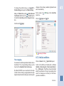
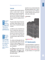
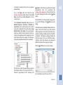
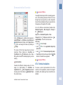
Download FEFLOW® 6.1

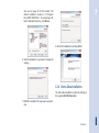
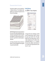
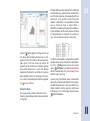
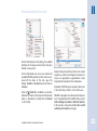
DHI-WASY Software
FEFLOW 6.1
®
Finite Element Subsurface Flow
& Transport Simulation System
Installation Guide & Demonstration Exercise
Copyright notice:
No part of this manual may be photocopied, reproduced, or translated without written permission of
the developer and distributor DHI-WASY GmbH.
Copyright © 2012 DHI-WASY GmbH Berlin – all rights reserved.
DHI-WASY, FEFLOW and WGEO are registered trademarks of DHI-WASY GmbH.
DHI-WASY GmbH
Waltersdorfer Straße 105, 12526 Berlin, Germany
Phone:
+49-(0)30-67 99 98-0,
Fax:
+49-(0)30-67 99 98-99
E-Mail:
[email protected]
Internet: www.feflow.com
www.dhigroup.com
2
3
Contents
I Installation Guide
4
II.2
Getting Started
14
I.1
I.2
Introduction
Installing FEFLOW (Windows)
4
5
II.2.1
II.2.2
Starting FEFLOW
FEFLOW 6.1 User Interface
14
14
I.2.1
I.2.2
I.2.3
I.2.4
I.2.6
5
5
6
7
II.3
Geometry
15
II.3.1
II.3.2
II.3.3
II.3.4
Maps and Model Bounds
Supermesh
Finite element-mesh
Expansion to 3D
15
16
18
19
I.2.7
Introduction
System recommendations
FEFLOW Installation
Demo Data Installation
Installation of the Network
License Manager NetLM
License installation
8
8
I.3
I.4
Installing FEFLOW (Linux)
Installation Packages
9
9
II.4
II.5
Problem settings
Model Parameters
25
27
II.5.2
II.5.3
Boundary conditions
Material properties
27
34
II.6
II.7
Simulation
Flow and Transport Model
37
40
II.7.1
II.7.2
II.7.3
II.7.5
II.7.6
II.7.7
II.7.8
Problem settings
Initial conditions
Horizontal Refinement
Material properties
Vertical resolution
Simulation Run
Postprocessing
40
41
42
44
46
48
49
II Demonstration Exercise
11
II.1
Introduction
11
II.1.1
II.1.2
II.1.3
II.1.4
II.1.5
About FEFLOW
Scope and Structure
Terms and Notations
Requirements
Model Scenario
11
11
12
12
13
More Information
52
FEFLOW 6.1
I Installation Guide
I.1
Introduction
The FEFLOW simulation package contains the following main programs along with additional software tools:
FEFLOW® 6.1
FEFLOW is an interactive finite-element simulation
system for modeling 3D and 2D flow, mass and
heat transport processes in groundwater and the
vadose zone.
FEFLOW is provided on DVD for the following
platforms:
32-bit operating systems
• Windows XP, Vista, 7, Server 2003, Server 2008
• Linux: CentOS 5.1 (RedHat family), OpenSUSE
11.0 (SUSE family), Ubuntu 10.04 (Debian family)
64-bit operating systems
• Windows XP x64 Edition, Vista x64 Edition,
7 x64 Edition, Server 2003 x64 Edition,
Server 2008 x64 Edition
• Linux: CentOS 5.1 (RedHat family), OpenSUSE
11.0 (SUSE family), Ubuntu 10.04 (Debian family)
Installation Guide & Demonstration Exercise
FEFLOW for other Linux distributions may be available for download from the FEFLOW website
www.feflow.com. If you need FEFLOW for another
Linux distribution, please do not hesitate to contact us at [email protected]!
For evaluation purposes, it is possible to obtain a
fully functional but time-limited license from DHIWASY, one of the DHI offices, or from your local
FEFLOW distributor.
FEFLOW® Viewer
FEFLOW Viewer is free software for visualizing
FEFLOW models and results and for postprocessing purposes. FEFLOW Viewer is installed with
FEFLOW.
WGEO® 6.0
WGEO® is a sophisticated georeferencing,
geoimaging and coordinate transformation software developed by DHI-WASY GmbH. A license
for WGEO® Basis and the flexible 7-parameter
transformation comes with each FEFLOW license
and is installed automatically.
WGEO® is provided for the Windows platform.
4
I.2
5
Installing FEFLOW
(Windows)
I.2.1 Introduction
FEFLOW 6.1 provides powerful state-of-the-art
editing, visualization and evaluation tools as well
as computational methods for most kinds of
groundwater models.
To run FEFLOW in single-seat mode, the DHI-WASY
License Manager NetLM has to be installed locally.
If the the license shall be acquired from a license
server using a network connection (network license
required), no local installation of NetLM is necessary.
A license server can be set up by installing NetLM
on that machine. The installation of FEFLOW on
the same computer is not necessary.
A typical FEFLOW installation on a Windows operating system consists of three steps:
• Installation of FEFLOW and additional programs
• Installation of the demo data package
• Installation of the DHI-WASY license manager
NetLM
After inserting the DVD into the DVD drive, an
overview of the DVD contents is shown automatically. If autostart is disabled, run Starter.exe from
the windows directory on the DVD.
The hyperlinks in the overview can be used to start
the different parts of the FEFLOW installation, to
view the documentation and example movies, and
to install third-party software.
FEFLOW is automatically installed as a 32 bit version on 32 bit systems, and as 32 and 64 bit versions on 64 bit operating systems.
I.2.2 System recommendations
The following system specifications are recommended as a minimum configuration. The
memory requirements depend on the size and
complexity of the actual model to be simulated.
FEFLOW 6.1
I
I
Installation Guide
• 512 MB RAM
• 250 MB of disk space
• Dedicated graphics card with up-to-date graphics driver
I.2.3 FEFLOW Installation
Start the Windows Installer by clicking on the
hyperlink FEFLOW Program Files. Click Next after
each step to proceed to the next step.
1. A Welcome screen appears first.
4. In the License window, choose Demo for testing
FEFLOW without a license. Select Client if the
license to be used is installed on a remote
license server (Network License) and type in the
name or IP number of the license server. Choose
Server if a Single Seat License is to be used or if
the machine is intended to act as a license server
for a Network License.
2. In the next step, the License Agreement has to
be accepted. Please read it carefully before proceeding with the installation.
3. Wait until the installer has determined the available disk space.
5. Select the packages to install. Details about the
packages can be found on the right of the winInstallation Guide & Demonstration Exercise
6
7
dow and on page 10 of this booklet. The
default installation location is C:\Program
Files\WASY\FEFLOW 6.1. For specifying a different destination directory, click Browse.
8. Finish the installation by clicking Finish.
6. Start the installation or go back to change the
settings.
I.2.4 Demo Data Installation
The demo data installation is started by clicking on
the hyperlink FEFLOW Demo Data.
7. FEFLOW is installed. This may take several minutes.
FEFLOW 6.1
I
I
Installation Guide
I.2.6 Installation of the Network
License Manager NetLM
Before installing the Network License Manager
NetLM we recommend to deinstall all previous
versions of NetLM.
The installation is started by clicking on the hyperlink License Manager NetLM. Follow the instructions
in the installation dialog.
I.2.7 License installation
There is only one
dongle for each
copy of FEFLOW.
If the dongle is lost, it can
only be replaced by purchasing a new license of
FEFLOW!
This step can be skipped for working in Demo
mode only. All license installations have to be done
with administrator privileges.
Make sure that the firewall allows (local) TCP/IP
connections on port 1800.
• Attach the dongle (hardware lock) to the USB
port. Start the DHI-WASY License Administration
tool by clicking on the WASY License
Administration entry in the All Programs\WASY
group of the Windows start menu.
• In the tree view on the left side, select Dongle
license in the FEFLOW 6.1 branch. In the
Hostname or IP address field, insert localhost if
the dongle is installed locally, or insert the name
or the IP number of the remote license manager.
• Click Connect. Check whether the number
returned in the field HOSTID is identical to the
number on the FEFLOW license sheet. In case
that multiple dongles of the same brand are
connected, a HOSTID mismatch may occur. In
this case remove all dongles except the DHIWASY dongle.
• Switch to the Licenses tab and enter the license
information from the FEFLOW license sheet.
Installation Guide & Demonstration Exercise
8
For the 64 bit version of FEFLOW, a
HASP HL USB
dongle is required. If you do
not already have such a
dongle, please contact your
FEFLOW distributor or DHIWASY for a dongle
exchange!
The license information can be pasted from the
clipboard if the license has been received digitally. Copy the selected section in the license
document to the clipboard and use the Paste
license from clipboard button to insert all the
license information at once. Please also make
sure that the same license type as on the license
sheet is selected:
• Single seat license – FEFLOW can be run only
on the computer the dongle is attached to.
For the version,
please note that
you have to use
“6.1x” because your license
is valid for all sub-versions
of FEFLOW 6.1.
• Network license – FEFLOW can be used on any
computer connected to the license server via
TCP/IP network (LAN or WAN/internet).
• Click Install. A message box indicates that the
license has been successfully installed. If the
installation was not successful, check all the
license information in comparison to the information provided on the license sheet. The information has to be identical in all details.
• Click OK to close the License Administration dialog.
• Choose FEFLOW 6.1 from the WASY program
group or double click on the desktop icon to
start FEFLOW.
I.3
9
Installing FEFLOW
(Linux)
• Browse to the linux directory on the DVD.
• Browse to the sub directory corresponding to
your Linux distribution.
• For a full installation, use the following command: rpm -i *.rpm
• For deinstalling all WASY packages, use rpm e ‘rpm -qa | grep ’^wasy-’‘
• Note that you may need root privileges to perform these commands.
I.4
Installation Packages
• Packages for installation can be selected during
the first installation or by re-running the installation in Modify mode.
• A description for each package is shown in the
right part of the Select feature dialog of the
installation by selecting one of the packages.
• The following packages are available:
Using a Network License for FEFLOW, the WASY
License Manager can be installed on any computer
within the network (LAN or WAN) without the
complete FEFLOW installation. Clients need TCP/IP
connection on port 1800 to have access to the
license server.
FEFLOW 6.1
I
Installation Guide
FEFLOW
Data Tools
FEFLOW program files - required for running
FEFLOW
Scripts for data checking and format conversion.
• Help - FEFLOW help system
• Interface Manager SDK - development kit for
the open programming interface IFM (required
for plug-in development)
• Desktop shortcut icons on the Windows desktop
WGEO Basis is
licensed automatically with
FEFLOW. If a license dialog
show up, just click on
Cancel.
I
In the demo data installation there are the following packages:
• Examples - example models
• Exercise - data for the demonstration exercise
WGEO
• Tutorial - data for the tutorials (User Manual)
Georeferencing, geoimaging and transformation
software - a WGEO license is installed automatically.
• Benchmarks - benchmark models
• WGEO help - online help system
• German Transformations - coordinate transformation routines for Germany (may require separate licensing)
• Desktop shortcut icon - WGEO icon on the
Windows desktop
Plot Assistant
GIS-like software for producing plots with FEFLOW
data.
Installation Guide & Demonstration Exercise
10
11
II Demonstration Exercise
II.1
Introduction
II.1.1 About FEFLOW
FEFLOW (Finite Element subsurface FLOW and
transport system) is an interactive groundwater
modeling system for
• three-dimensional and two-dimensional
• areal and cross-sectional (horizontal, vertical or
axisymmetric)
• fluid density-coupled, also thermohaline, or
uncoupled
• variably saturated
• transient or steady state
• flow, mass and heat transport
• reactive multi-species transport
in subsurface water resources with or without one
or multiple free surfaces.
FEFLOW can be efficiently used to describe the
spatial and temporal distribution and reactions of
groundwater contaminants, to model geothermal
processes, to estimate the duration and travel
times of chemical species in aquifers, to plan and
design remediation strategies and interception
techniques, and to assist in designing alternatives
and effective monitoring schemes.
Sophisticated interfaces to GIS and CAD data as well
as simple text formats are provided.
The option to use and develop user-specific plugins via the programming interface (Interface
Manager IFM) allows the addition of external code
or even external programs to FEFLOW.
FEFLOW is available for WINDOWS systems as well
as for different Linux distributions.
Since its first appearance in 1979 FEFLOW has
been continuously extended and improved. It is
consistently maintained and further developed by
a team of experts at DHI-WASY. FEFLOW is used
worldwide as a high-end groundwater modeling
tool at universities, research institutes, government
agencies and engineering companies.
For additional information about FEFLOW please
do not hesitate to contact your local DHI office,
one of the FEFLOW distributors, DHI-WASY, or
have a look at the FEFLOW web site
http://www.feflow.com.
II.1.2 Scope and Structure
This exercise provides a step-by-step description
of the setup, simulation, and post processing of a
three-dimensional flow and transport model based
on (simplified) real-world data, showing the
philosopy and handling of the FEFLOW user interface.
FEFLOW 6.1
Demonstration Exercise
You can skip any
of the steps in this
exercise by loading
already prepared files at
certain stages. These files
are not necessarily ready to
run in the simulator.
The demonstration exercise is not intended as an
introduction to groundwater modeling itself.
Therefore, some background knowledge of
groundwater modeling is required, or common
literature should be consulted in parallel.
The exercise covers the following work steps:
• Definition of the basic model geometry
• Generation of a 3D finite-element mesh
• Setup of a transient transport model, including
initial conditions, boundary conditions and
material properties
• Import of GIS data and regionalization
• Simulation run
• Results visualization and post processing
II.1.3 Terms and Notations
For following the
exercise, the demo
data files for
FEFLOW have to be installed. The demo data installation package is available
on the FEFLOW DVD as
well as on the FEFLOW web
site for download.
In addition to the verbal description of the required
screen actions this exercise makes use of some
icons. They are intended to assist in relating the
written description to the graphical information
provided by FEFLOW. The icons refer to the kind
of setting to be done:
main menu
context menu
toolbar
panel
Installation Guide & Demonstration Exercise
button
input box for text or numbers
switch toggle
radio button
checkbox
II
All file names are printed in bold red, map names
are printed in red italic and numbers or text to be
entered by the user in bold green. Keyboard keys
are referenced in <italic> style. All required files are
available in the FEFLOW demo data. The
symbol indicates an intermediary stage where
either a prepared file can be loaded to resume this
exercise or - if working with a license - the model
can be saved. Thus the exercise does not have to
be done in one step even in demo mode.
II.1.4 Requirements
If not already done, please install the FEFLOW software including the demo data package. A license is
not necessary to run this tutorial (FEFLOW can be run
in demo mode).
The latest version of FEFLOW can be downloaded
from the website www.feflow.com. In case of any
problems or additional questions please do not hesitate to contact the FEFLOW technical support
([email protected]).
12
II.1.5 Model Scenario
A fictitious nitrate contaminant has been detected
near the small town of Friedrichshagen, in the
southeast of Berlin, Germany. An increasing concentration can be observed in two water supply
wells. There are two potential sources of the contamination: The first are abandoned sewage fields
close to a waste-water treatment plant located in
an industrial area northeast of town. The other
possible source is an abandoned waste-disposal
site further east.
A three-dimensional groundwater flow and contaminant transport model is set up to evaluate the
overall threat to groundwater quality, and to quantify the potential pollution. First, the model domain
needs to be defined. The town is surrounded by
many natural flow boundaries, such as rivers and
lakes. There are two small rivers that run northsouth on either side of Friedrichshagen that can
act as the eastern and western boundaries. The
lake Müggelsee can limit the model domain to the
south. The northern boundary is chosen along an
northwest-southeast hydraulic contour line of
groundwater level north of the two potential
sources of the contamination.
13
The geology of the study area is comprised of
Quaternary sediments. The hydrogeologic system
contains two main aquifers separated by an
aquitard. The top hydrostratigraphic unit is considered to be a sandy unconfined aquifer up to 7
meters thick. The second aquifer located below
the clayey aquitard has an average thickness of
approximately 30 meters.
The northern part of the model area is primarily
used for agriculture, whereas the southern portion
is dominated by forest. In both parts, significant
urbanized areas exist.
FEFLOW 6.1
II
Demonstration Exercise
II.2
Getting Started
II.2.1 Starting FEFLOW
On Windows Systems
• Start FEFLOW 6.1 via the corresponding desktop icon or the startup menu entry.
On Linux Systems
• Type feflow61q in a console window and press
<Enter> .
If no FEFLOW license is available, FEFLOW asks
whether to start in demo mode. The demo mode
does not allow loading and saving of files with
more than 500 nodes. Specially prepared demo
files coming with FEFLOW are an exception. Such
files are provided for this example so that the
model setup can be interrupted and picked up
again.
and
View > Panels, respectively. Please keep in
mind that not all panels and toolbars are displayed
by default. Thus this exersice may require to access
a function in a toolbar or panel that is not visible
at that moment. The toolbar or panel has to be
added then.
II
During the work with FEFLOW models, view windows display a certain type of view on the model
and its properties. There are different types of view
windows: Supermesh view, FE-Slice view, 3D view,
Cross-Section view and Data-Trace view. The availability of different functionality like toolbars
depend on the currently active view type.
View windows can be closed via the corresponding button in the view frame. New view windows
can be opened by selecting
Window > New
and choosing the respective view window type.
II.2.2 FEFLOW 6.1 User Interface
The user interface components are organized in a
main menu, toolbars, panels, view windows, and
dialogs.
While the main menu is always visible, the other
parts of the interface can be customized, adding
or hiding particular toolbars and panels by using
the menu command
View > Toolbars
Installation Guide & Demonstration Exercise
The last type of user interface component relevant
for the exercise are charts. Looking very similar to
panels, they contain plots of time curves. Missing
chart windows can be added to the user interface
14
In this exercise,
different file types
are used as data
source at the different
stages of modelling to
show the number of
options. In practical projects, it may be preferred to
store basic data in one file
type, e.g., shp when using
GIS.
by opening
View > Charts from the menu and The particular map files that are needed now are:
choosing the required chart type from the list.
• topography_rectified.tif (a georeferenced raster
image of the model area for better orientation)
Last, but not least it might be worth to mention
that all steps done in FEFLOW can be undone and • model_area.shp (a polygon map that contains
several polygons denoting the outer model
redone via the corresponding toolbar buttons.
boundary and embedded contamination areas)
There is no limit on the number of undo steps.
II.3
Geometry
II.3.1 Maps and Model Bounds
After opening FEFLOW, start a new model by
File > New or the
using the menu command
New button in the
Standard toolbar.
15
• contamination_sources.dxf (the footprint of the
sewage fields and the waste disposal as polygons)
• wells.shp (the positions of the wells)
Some of these maps will also be used for model
parameterization later on.
After import, the maps are listed in the Maps
The first step of model setup is the definition of panel, sorted by their file type (see figure). A double
the Initial Domain Bounds. This can be done man- click on the Geo-TIFF topography_rectified adds the
ually, or by loading georeferenced maps.
georeferenced topographic map to the active
Supermesh view window.
All necessary files for this exercise are provided with
the FEFLOW Demo Data package and are located
in the project folder demo/exercise. The map files
are found in the subdirectory import+export.
Click on
Multiple, possibly nonoverlapping maps
[...] and press
Finish. Load all the following
maps at once (by holding <Ctrl> on the keyboard)
to ensure that FEFLOW uses the bounding box of
all the maps to define the initial domain bounds.
You may have to select All Maps in the Files of Type
selector at the bottom of the dialog.
Except for the maps contamination_sources and topography_rectified all other maps are ESRI shape files.
These vector files occupy their own branch in the
FEFLOW 6.1
II
Demonstration Exercise
tree, each with a default map layer. Double-click on
all the Default layer entries to add the visualization
layers of the shape files to the Supermesh view.
Now have a closer look at a second panel, the
View Components panel. This panel lists the components that are currently plotted in the active view
window.
When loading the map layers to the view, the maps
have also been added to the tree in the
View Components panel.
of the mass sources). The topmost map is drawn
on top.
II
To switch a map on and off, the checkbox in front
of the map name can be checked/unchecked. If
checking/unchecking the checkbox of an entire
branch all the maps in this branch become visible/invisible at the same time.
The topographic map has mainly been loaded for
providing a regional context. For more clarity, it
can be switched off before starting with the following operations. Make sure that the other maps
are visible.
II.3.2 Supermesh
In the simplest case, the supermesh contains a definition of the outer model boundary. In addition,
geometrical features such as the position of pumping wells, the limits of areas with different properties or the courses of rivers can be included to
be considered for the generation of the finite-element mesh. Additionally, the polygons, lines and
points specified in the supermesh can be used later
on to assign boundary conditions or material properties.
The drawing order of maps can be modified by
dragging them with the mouse to another position in the tree (this might become necessary as
the model area polygon may overlay the polygons
Installation Guide & Demonstration Exercise
As mentioned above, a supermesh may contain
three types of features:
• polygons
• lines
• points
16
At least one polygon has to be created to define
the model area boundaries.
The editing tools are found in the
toolbar:
Mesh Editor
Outer boundary and contamination
sources
Before generating the finite-element mesh, the
well locations are to be included in the supermesh
for this example.
17
Well locations
The positions of the wells can be imported directly
from a map as well. Open the context menu of
the map wells in the
Maps panel and choose
Convert to > Supermesh Points.
The polygons can be directly loaded from the map
model_area. In the
Maps panel, open the context menu of this map (with a right-click on the
map name) and choose
Convert to >
Supermesh Polygons.
The points immediately appear as red dots in the
Supermesh view.
The supermesh imported from the map does consist of several adjacent, non-overlapping polygons.
For additional editing, different tools are available
to manually modify the supermesh.
FEFLOW 6.1
II
Demonstration Exercise
For this example, choose
Gridbuilder. Click
Generate Mesh to start mesh generation.
II
A new Slice view is automatically opened, depicting the resulting finite-element mesh.
For our purpose, especially for the simulation of
contaminant transport, this initially generated
mesh does not seem to be appropriate. A finer spatial resolution is required.
Activate the Supermesh view again so that the
Mesh Generator and
Supermesh toolbar
become visible again.
exercise_fri1.smh
II.3.3 Finite element-mesh
Once the outer boundary and other geometrical
constraints have been defined in the supermesh,
the finite-element mesh can be generated.
All necessary tools can be found in the
Mesh Generator toolbar.
First, one of the mesh generation algorithm provided by FEFLOW is chosen from the drop-down
list in the
Mesh Generator toolbar.
Installation Guide & Demonstration Exercise
In the
Mesh Generator toolbar, enter
3000
as Total Elements and click
Generate Mesh again.
The finite-element mesh in the Slice view is
updated, showing a finer discretization now.
Local refinement
At the pumping wells steep hydraulic gradients are
expected at the center of the well cone. To realistically represent these, fine discretization is necessary, too.
Switch to the Supermesh view again to see the
Mesh Generation toolbar. If the view has been
accidentally
closed,
re-open
it
by
choosing
Window > New > Supermesh View
from the menu.
18
Zooming functions can be used
at any time. Press
and hold the right mouse
button, move the mouse
up/down). Pan by pressing
and holding the mouse
wheel and moving the
mouse to any direction.
Also the mouse wheel may
be used for zooming.
19
Click on
Generator Properties to open the
Generator Properties dialog.
Besides refinement at points or
polygon borders,
FEFLOW also provides the
means to edit the desired
relative mesh density on a
polygon-by-polygon basis.
To obtain a refinement around the well locations,
activate the
Point element gradation. Apply a
refinement level of 10.
Leave the dialog by clicking on
OK.
Click
Generate Mesh one last time and check
the changes in the mesh. The refinement pattern
looks similar to the one in the figure where the
mesh around the well locations is finer.
exercise_fri1.fem
II.3.4 Expansion to 3D
Up to this point we have worked on the model
seen in top view, not considering the vertical direction. Starting from this 2D geometry, a 3D model
consisting of several layers is set up.
The actual elevation of the layers tops and bottoms is derived by an interpolation based on map
data (point-based data).
For this example, three geological layers are considered for the model. An upper aquifer is limited
by the ground surface on top and by an aquitard
at the bottom. A second aquifer is situated below
FEFLOW 6.1
II
Demonstration Exercise
the aquitard, underlain by a low permeable unit
of unknown thickness. This underlying stratigraphic layer is assumed to be impervious and is
not part of the simulation.
FEFLOW distinguishes between layers and slices in
3D. Layers are three-dimensional bodies that typically represent geological formations like aquifers
and aquitards. The interfaces between layers, as
well as the top and bottom model boundary are
called slices.
In a first step, the numbers of layers and slices are
defined. The actual stratigraphic data are applied
in a separate step afterwards.
Installation Guide & Demonstration Exercise
Initial 3D Setup
Open
II
Edit > 3D Layer Configuration.
In the upper left corner of the dialog, a text field
shows the current number of layers (1). Increase
this value to
3 and hit <Enter>. This makes
FEFLOW switch the model geometry to 3D, the
model containing 3 layers. The number of slices
automatically changes to 3 + 1 = 4 . By default,
the top slice has a spatially constant elevation of
0 m. The other slices are placed below with a distance of 1 m each.
20
The basic data have been derived from a DEM and
from borehole logs, and have been combined into
a text file (extension dat, tab separated) with four
columns: X, Y, Ele, and Slice. Such a file can be
edited in a text editor, or in spreadsheet software
such as Microsoft Excel or Open Office /
LibreOffice. Containing the target slice number as
a point attribute, the file can be used as the basis
for regionalization of elevations for all slices at
once. The elevations are given in meters ASL.
Click on
OK to apply the settings and to exit
the dialog. After finishing the basic layer configuration of the 3D model, a 3D view automatically opens. This view shows the actual 3D
geometry of the model, now containing 4 planar
slices with a distance of 1 m each. The 3D view
background by default is set to black. To achieve
better visibility in print, for all images in this exercise a white view background has been applied.
exercise_fri2.fem
Elevation Data
This raw geometry will be formed into its real
shape by regionalizing elevation data contained
in map files.
21
The file has to be loaded as a map before its attribute data can be used as the basis for interpolation.
Go to the
Maps panel and use the context
menu (
Add Map(s)...) to add elevations.dat to
the list of loaded maps. It is not necessary to visualize the map in the view.
As a next step, the attribute values of the data file
need to be associated with (linked to) their respective FEFLOW parameter, in this case with the elevation. In order to do this, open the context menu
of the map elevations with a right click and choose
Link to Parameter….
FEFLOW 6.1
II
II
Demonstration Exercise
On the left-hand side of the dialog, the available
attributes of the map are listed. Select the entry
Ele with a mouse click.
On the right-hand side, a tree view contains all
available FEFLOW parameters that can be associated with the data. In this tree, open the
Process Variables > Elevation branch and click on
Elevation.
Click on
Add Link to establish a connection
between the values in the map and the elevation
data, or - alternatively - double click on Elevation
to set the link.
Installation Guide & Demonstration Exercise
Besides linking the attribute field to the model
properties, a number of settings has to be done to
ensure an appropriate regionalization when
importing the map data to the nodal values.
By default, FEFLOW expects elevation data to be
in the unit meters, which is correct in this case.
FEFLOW only applies two-dimensional interpolation. To separate data for the different slices, select
Field containing slice number in Node/Slice Selection.
In the next line, choose the attribute Slice as Field
containing slice number (see image).
22
23
To transfer data from the points in the map to all
the mesh nodes, a regionalization method has to
be applied. From the dropdown menu for Data
Regionalization Method in the lower part of the dialog, choose the
Akima method. As the properties, set:
• Interpolation type:
Linear
• Neighbors:
3. Only the three map points
that are closest to a mesh node are used for the
interpolation.
• Over-/Under Shooting:
0. Thus the resulting
values may not exceed the range of input values.
Click on
OK to apply these settings and to
close the dialog.
This can be done in the
(
View > Panels).
Navigation panel
Click on the tab Projection and move the Scaling
slider bar upwards until you have achieved a convenient view on the 3D model. Alternatively, the
<Shift> key in combination with the mouse wheel
also changes the stretch factor for the active 3D
view.
Elevation data assignment
Click into the 3D view to bring it to front. Make
sure to have the
Rotate tool in the
View
toolbar activated. Rotation, panning, and zooming can be easily performed using the mouse:
• Left mouse button: rotate the model around its
center of gravity
• Center mouse button (mouse wheel): pan the
model (left/right/up/down)
• Right mouse button: zoom (in/out)
As the model has a rather small vertical extent
compared to its horizontal dimensions, the (vertical) z-axis should be exaggerated.
FEFLOW 6.1
II
Demonstration Exercise
As a next step, the target locations of the data
assignment have to be defined, i.e., all nodes in
the mesh have to be selected.
• Click on
bar.
Select All in the
Selection tool-
II
To finally assign the elevation data by regionalization from map data to the selected nodes, two
more steps are required:
• In the
Maps panel, open the branch Maps
> ASCII Table Files > elevation. Under
Linked Attributes, double-click on Ele -> Elevation.
• Click
Assign in the
Editor toolbar to apply
the new elevation data to all nodes.
In the 3D view the node elevations are immediately updated.
Editor toolbar, the map ele• Hereby, in the
vation is automatically set as data source in the
input box and the model property Elevation is
activated as parameter. Note that also Elevation
has been chosen in the
Data panel and is
now shown in bold letters.
Installation Guide & Demonstration Exercise
Click on
bar.
Clear Selection in the
Selection tool-
The result looks as shown in the figure below.
Probably the Scaling has to be adjusted again
(
Navigation panel > Projection tab or <Shift> mouse wheel) to account for the changed vertical extent.
24
25
exercise_fri3.fem
II.4
Problem settings
FEFLOW provides the means to simulate a number of different physical processes in different spatial and temporal dimensions, ranging from simple
2D steady-state flow models to transient, unsaturated, density-coupled reactive transport models.
As the input parameters depend on the model
type, the general problem settings are typically
done in the beginning.
Go to
Edit > Problem Settings to open the
Problem Settings dialog, where all general settings
related to the current model are done.
All these settings are organized in thematic pages
controlled by a tree view on the left-hand side of
the dialog.
Problem class
The principal type of the FEFLOW model is defined
on the Problem Class page.
Below the Scenario description (which is not
mandatory to be modified) one of two general
types of problems – saturated media and unsaturated/variably saturated media is chosen.
By default Standard (saturated) groundwater flow
equation is selected, applying Darcy’s equation.
Though this option is selected, the model is able
to account for phreatic conditions.
FEFLOW 6.1
II
Demonstration Exercise
Additional
selection options
are described in
detail in the FEFLOW help
system.
The second option - Richards’ equation (unsaturated or variably saturated media) - would lead to
Richards’ equation being applied, being capable
of accounting for both saturated and unsaturated
conditions within one model.
In this particular case, it is not expected that considering the unsaturated/variably saturated zone
would change the model result to an extent that
would justify the additional effort for the solution.
Keep the default setting (Standard groundwaterflow equation) for this exercise.
heat transport processes to the always executed
flow simulation.
II
However, activating the transport option now
would increase the complexity to an extent that
is not necessary at this stage. Thus we first focus
on the flow model and add mass transport at a
later stage.
The flow model is set up for steady-state conditions, switch to
Steady.
Click on
Apply to apply the changes.
Free Surface
The first aquifer in the simulation area is known to
be unconfined, so a phreatic water table is to be
simulated. For this example, an approximation of
the phreatic level by applying a pseudo-unsaturated technology is chosen. Hereby, a reduced
conductivity is applied during the simulation to
model layers if they are located above the water
table. For more information on the handling of
free surfaces in 3D models, please refer to the help
system and FEFLOW Documentation.
On the same page, Problem class settings are done.
Besides choosing between transient and steadystate conditions, it is also possible to add solute or
Installation Guide & Demonstration Exercise
The settings for unconfined conditions are located
on the Free Surface page. First of all, switch to
Unconfined aquifers(s). In the Status column,
open the drop down list of Slice 1 and choose the
option
Phreatic.
26
For the slices 2 and 3 keep the option
Dependent (the status of the bottom slice 4 is
fixed and cannot be changed).
Finally, set the Residual water depth for unconfined
layers to a value of 0.05 m to account for the residual water content in the unsaturated zone. In this
way, finite elements above the water table have a
small residual conductivity. This allows modelling
a rerise of the water table and also increases the
numerical stability of the model.
Close the dialog by clicking
Apply and
OK.
exercise_fri4.fem
II.5
Model Parameters
In the following sections, the physical properties
of the study area are applied to the finite-element
model.
The respective parameters are found in the
Data panel. The parameters are organized in
the following main branches in the tree view:
• Process Variables
• Boundary Conditions
• Material Properties
• Auxiliary Data
• User Data
• Discrete Elements
II.5.2 Boundary conditions
To calculate the hydraulic head distribution
between the upstream and downstream boundary, appropriate boundary conditions are applied.
For the sake of simplicity, they will be kept in a
rather simple way:
27
• Southern border: The lake Müggelsee completely controls the head along the southern
boundary. The lake water level of 32.1 m is used
as the value for a 1st kind (Dirichlet) hydraulichead boundary condition.
• Northern border: As there is no natural boundary condition like a water divide close to the
boundary, a head contour line will be used
instead (hydraulich head = 46 m).
• Western and eastern border: Two small rivers
(the Fredersdorfer Mühlenfließ and the
Neuenhagener Mühlenfließ) form the boundaries at the western and eastern limits of the
model. As they follow roughly the groundwater flow direction, we assume these heavily
clogged creeks to represent boundary streamlines. No exchange of water is expected over
this boundary and therefore a no-flow boundary condition is assumed.
• Finally, two wells, with a pumping rate of
900 m³/d and 1,000 m³/d, respectively, are
located in the southern part of the model. These
represent a number of large well fields in reality.
FEFLOW 6.1
II
Demonstration Exercise
The hydraulic head boundary conditions are
entered manually, while the wells are derived from
a map.
Manual editing is often easier if being done in a
2D view. Thus switch to the Slice view. If you have
accidentally closed it, a new view can be opened
via
Window > Slice view.
Northern Boundary
II
Zoom to the northern boundary.
For the Slice view, the
Selection toolbar provides additional tools for selecting nodes compared
to the 3D view. Choose
Select Nodes Along a
Border.
Slice view
This view type always shows a single slice or layer.
Browsing between the slices is easiest by hitting
the <Pg Up> and <Pg Down> keys, respectively.
Alternatively, the layer/slice to be seen in the view
can be directly selected in the
Spatial Units
panel.
The recommended tool for navigation in the Slice
view is the
Pan tool in the
View toolbar. The
mouse buttons are associated with the following
functions:
• Left and center mouse button: pan
• Right mouse button: zoom (in/out)
• Mouse wheel: zoom (in/out) in steps
Installation Guide & Demonstration Exercise
Having this tool selected, click on the westernmost
node of the boundary and hold down the left
mouse button, move the mouse cursor to the easternmost node and release the button. The nodes
of the northern border are highlighted as yellow
points. The selection is shown in the 3D view
simultaneously.
28
29
Go to the
Data panel and double-click on
Boundary Conditions (BC) > Fluid flow > Hydraulichead BC, the type of boundary condition to be
applied.
Next, the selection is extended to the other three
slices of the model. A time-saving way to do this is
the application of the
Copy Selection to
Layers/Slices tool. Start the tool and select all slices
in the upcoming dialog (manually or by hitting
<Strg>-<A>). Click on
OK.
Bring up the 3D view and ensure that indeed all
nodes at the northern boundary are selected.
To manually assign a hydraulic-head boundary
condition make sure that the Assign Values method
is active in the
Editor toolbar (see figure). If
not, open the context menu by a right click on the
symbol in the input box and choose
Assign
Values.
FEFLOW 6.1
II
Demonstration Exercise
Enter
toolbar
button.
46 m in the input box of the
and
click
on
the
After defining the
boundary condition
at the northern
boundary, we store
the current selection
for later use:
Editor
Assign
Blue circles appear around the selected nodes to
indicate the Hydraulic-head BC. While having the
3D view active, double-click on Hydraulic-head BC
in the
Data panel to also show the boundary
conditions in 3D.
The values of the boundary condition can be
checked using the inspector tool, which is activated by clicking on
Inspect nodal/elemental values in the
Inspector toolbar. Move the
hair-cross to a node with a boundary condition.
The values of all properties currently visible in the
active view are shown in the
Inspection panel.
II
Open the context
menu
of
the
Spatial Units
panel and choose
Store
Current
Selection (will appear
in the
Spatial
Units panel as Node
Selection #1). To give this selection a recognizable
name, choose
Rename from its context menu
and change the name to
Northern
Boundary.
Afterwards, it is important to select (click on)
Domain in the
Spatial Units panel again. This
will make sure that any model properties are plotted on the entire model domain later.
Click on
Clear selection.
The inspector tool can be closed by hitting <Esc>
or by activating another tool (e.g.,
Rotate) in
the
View toolbar.
Installation Guide & Demonstration Exercise
30
31
Southern Boundary
The assignment of boundary conditions along the
southern boundary is done in the same way:
• In the Slice view, zoom/pan to the southern border.
•
Select nodes along a border.
•
Copy selection to all slices.
• Switch to the 3D view and check that the
selection is set correctly.
• Make sure that
Hydraulic-head BC in the
Data panel is still active.
• Store the selection and rename it to
Southern Boundary for later use.
• Select (click on) Domain in the
panel.
•
Spatial Units
Clear selection afterwards.
exercise_fri5.fem
Remaining outer boundaries
At nodes without an explicit boundary condition,
FEFLOW automatically applies a no-flow condition.
Therefore, no further action is required for the
western, eastern, top and bottom model boundaries, which are assumed to be impervious except
for groundwater recharge to be added later.
Pumping wells
The wells are to be set in the southern part of the
study area based on the map wells. They are
assumed to be screened throughout the whole
depth of the model.
• Type
32.1 m in the input box of the
Editor toolbar and click
Assign.
This kind of well, which stretches along a number
of layers, is called a multilayer well. Multilayer wells
are assigned along vertical element edges (called
Join Edges). Nodes along these edge selections are
connected automatically by a high-conductive
finite element that mimics the borehole.
FEFLOW 6.1
II
II
Demonstration Exercise
Several parameters are necessary to assign a multilayer well, including the pumping rate, the radius
of the well and elevation of the top and bottom
end of the screen.
While it is also possible to manually enter these
values, it is more convenient to import them from
a map.
The wells map contains attribute data that need to
be associated with (linked to) their respective
FEFLOW parameter. In order to do this, open the
context menu of the map wells (in the
Maps
Link to
panel) with a right click and choose
Parameter… to open the Parameter Association dialog.
Repeat these steps for the attribute fields
On the left-hand side of the dialog, you see the
available data of the map.
• RADIUS
(link to Radius)
• SCREENTOP
(link to Top elevation)
The attribute CAPACITY relates to the abstraction
rate of the well, select it with a mouse click.
• SCREENBOTT
(link to Bottom Elevation)
• NAME
(link to Name).
On the right-hand side, open the Boundary
Conditions > Fluid Flow > Multilayer Well branch and
click on Type > Rate.
Click on
Add Link to establish a connection
between the values in the map and the Multilayer
well or double click on Rate to set the link.
Installation Guide & Demonstration Exercise
Each well will be created along that edge that is
closest to its corresponding data point, but still
within a user-defined search radius (snap distance).
The Snap Distance should be small but greater than
zero. enter
0.01 meters in the input field. Click
the
OK to close the dialog.
The actual assignment is done in a similar way
already performed while importing the elevation
data.
32
• In the
Maps panel, open the branch Maps
> ASCII Tables > wells. Under Linked Attributes,
double-click on -> Multilayer Well.
All boundary conditions are shown in the view.
Faces in
Uncheck the checkbox of Geometry >
View Components panel to see into the
the
domain.
33
Blue circles are shown on the northern and southern border, and four red symbols for each well.
• Click on
bar.
Select All in the
Selection tool-
• Click on
Assign in the
Editor toolbar. Even
though all nodes have been selected, the multilayer wells will be assigned each to the closest
node only.
exercise_fri6.fem
Finally check all boundary conditions you have set.
Clear the selection and go to the 3D view.
Make sure that Domain is selected in the
Spatial Units panel. Double-click on Boundary
Data panel.
Conditions (BC) > Fluid flow in the
exercise_fri7.fem
FEFLOW 6.1
II
Demonstration Exercise
II.5.3 Material properties
Top Aquifer (Layer 1)
• In the
Data panel, right-click on In/Outflow
on top/bottom and choose
Set Unit > mm/a
from the context menu.
In the top aquifer, the hydraulic conductivity, the
porosity as well as the groundwater recharge are
to be set.
• Input a value of
195 mm/a into the box in
the
Editor toolbarand hit <Enter>.
Although groundwater recharge from a mathematical point of view is rather a boundary condition, it is handled as a material property in
FEFLOW. In a 3D model, the respective parameter
to be set is In/Outflow on top/bottom.
• Activate Drain/Fillable Porosity in the
panel with a double-click.
• Input a value of
The input procedures for material properties are
completely analogous to the ones for the boundary conditions; material properties however are
assigned to elements instead of nodes:
• Add the map conduc2d.trp to the
Maps
Add maps(s)). This shape file contains
panel (
point-based conductivity values for the top
aquifer in 10-4 m/s.
• Go to the 3D view.
• Reactivate the checkbox of Geometry >
Faces
in the
View Components panel again.
• Activate Material Properties > Mass Transport >
In/Outflow on top/bottom in the
Data panel
with a double-click.
• Choose the
Select Complete Layer/Slice tool
(in the dropdown selector on the left of the
toolbar) in the
Selection toolbar and select
all elements in the top layer by clicking on it.
II
The porosity is applied to the same selection by
Data
0.1 and hit <Enter>.
The hydraulic conductivity will be assigned by
interpolating data from field samples.
• Associate (
Link to Parameter…) the attribute
column Value to the FEFLOW parameter K_xx.
K_yy and K_zz will be calculated from K_xx and
assigned later).
• Choose
10-4 m/s as Source data unit
Akima,
• As a regionalization method, choose
Linear, with Neighbors
3 and
0%
Over-/Under Shooting. Activate the checkbox
Logarithmic. Close the dialog with the
OK button.
• Double-click on Conductivity > K_xx in the
Data panel.
Installation Guide & Demonstration Exercise
34
If the top layer is no longer selected, choose the
Select Complete Layer/Slice tool in the
Selection toolbar and select it.
• In the
Maps panel, double-click on
Linked Attributes > Value -> K_xx.
• Click the
ment.
• To finally assign the conductivity values, click
the
Assign button in the
Editor toolbar.
•
exercise_fri8.fem
OK button to finalize the assign-
Lower aquifer (Layer 3)
Repeat the same steps as for layer 2:
Clear selection and select the elements in the
third layer applying
Select Complete
Layer/Slice again.
• Choose
Assign Multiple... from the context
menu of Material Properties > Fluid Flow.
• Enter
2e-4 m/s for K_xx.
Aquitard (Layer 2)
• Enter
0.1 for the Drain-/fillable porosity.
In the second layer, we only need to assign constant values for the conductivity and drain-/fillable porosity.
Clear selection and select the elements in the
•
second layer applying
Select Complete
Layer/Slice again.
•
A very efficient way to assign multiple model
properties is by right-clicking on Material
Properties > Fluid Flow in the
Data panel and
Assign Multiple... from the context
choosing
menu.
In the following dialog,
• Enter
1e-6 m/s for K_xx (including the
unit!).
• Enter
•
0.15 for the Drain-/fillable porosity
Uncheck all other properties.
35
Uncheck all other properties.
• Click the
ment.
OK button to finalize the assign-
exercise_fri9.fem
Anisotropic hydraulic conductivity
While K_xx has been assigned already, K_yy and
K_zz will be derived from K_xx.
K_yy is equal to K_xx, it will be assigned using a
simple copy&paste procedure:
Select All elements in the 3D View.
•
• Choose
Copy... from the context menu of
Material Properties > Fluid Flow > Conductivity >
K_1m
• Double-click on Material Properties > Fluid Flow
> Conductivity > K_2m
FEFLOW 6.1
II
Demonstration Exercise
• Choose
Paste... from the context menu of
Material Properties > Fluid Flow > Conductivity >
K_2m
Besides manual assignment and data import,
FEFLOW allows to calculate model properties
from mathematical expressions. This will be used
for the vertical conductivity K_3m, which is
assumed to be 10% of the lateral conductivity
K_1m.
• Double-click on Material Properties > Fluid Flow
> Conductivity > K_3m
formula by a double click, or by directly typing
them into the formula using the keyboard.
For this particular operation, select and delete
the word “current” on the right hand side of the
equal sign. Afterwards, double-click on Material
Properties > Fluid Flow > Conductivity > CONDX in
the list on the right to insert it into the formula.
Afterwards, click on the multiplication symbol in
the toolbar on the top and finally type 0.1 on
your keyboard. The resulting expression (see figure) calculates the vertical conductivity as 10%
of the horizontal conductivity. Afterwards, press
Close button.
the
II
• Switch to the
Expression input method by
clicking on the icon in the input box of the
Editor toolbar or by right-clicking into the
box and selecting from the drop-down list.
Then double click on Current Expression. The
Expression Editor opens.
The Expression Editor is a tool to create arbitrary
mathematical expressions for various purposes.
At the top of the dialog several toolbars provide
basic mathematical operations. On the right
hand side there is a list of other model parameters that can be used within the formula. All
operations and parameters can be added to the
Installation Guide & Demonstration Exercise
To finally assign the new values, click the
Assign button in the
Editor toolbar.
Clear selection.
exercise_fri10.fem
36
Reference Field Data
To be able to compare the computed groundwater levels to measurements, a couple of observation points will be loaded into the model.
Go to the
Maps panel and use the context
menu
(
Add
Map(s)...)
to
add
observation_wells.dat to the list of loaded maps.
It is not necessary to visualize the map in the view.
Open the Slice view again if it has been closed.
Right-click on the map entry in the
Maps panel
and choose
Convert to ... > Observation Points
from the context menu. The map file contains
information about the location, slice number and
measured hydraulic head in the observation well.
As default headers are used in this example file,
the association of attributes to the properties of
the observation points works automatically and no
changes need to be done in the upcoming dialog.
Click the
OK button to proceed.
The now imported observation wells can be
shown by a double-click on Observation Points in
the
Spatial Units panel.
exercise_fri11.fem
II.6
Simulation
The flow part of the flow and transport model is
complete. By running the steady-state model, a
hydraulic head distribution will be computed that
will also act as initial condition for the following
transient simulation.
37
In case that FEFLOW is run in licensed mode, save
the model to be able to return to the initial properties later! If running FEFLOW in demo mode, this
model cannot be saved as the number of nodes
per slice exceeds the allowed maximum of 500.
Please use the prepared file exercise_fri11.fem in
this case.
Starting the simulator
To run the simulation, click
Simulator toolbar.
Start in the
As the model is unconfined, the system is solved
iteratively, taking into account that the saturated
thickness of unconfined layers depends on the
actual solution for hydraulic head. The Error Norm
History chart provides information about the
remaining error in each simulation iteration. The
simulation stops after eight iterations, the error
reaching values below the defined error criterion.
During and after the simulation, all visualization
tools in FEFLOW can be used to monitor and postprocess the simulation results.
Make sure to select Domain again in the
Spatial Units panel.
FEFLOW 6.1
II
Demonstration Exercise
It is recommended
to save the file
before starting
the simulation (if working
with a license). During the
simulation, the process
variables will change and
you would lose the initial
conditions of the model.
Go to the
Data panel and double-click on
Process Variables > Fluid Flow > Hydraulic head for
visualization of the resulting hydraulic head distribution.
In addition, go to the
Spatial Units panel and
select (single click) Model Locations > Observation
Points. Afterwards, double click Process Variables >
Fluid Flow > Hydraulic head in the
Data panel.
(To achieve better visibility in print, the element
edges have been removed in the figure).
Make sure to select Domain in the
panel afterwards.
II
To check whether the model indeed has reached
the steady state, the overall water balance is calculated. The
Rate-Budget panel provides the
means for this.
If it has been closed accidentally, open the
RateBudget panel via
View > Panels > Rate-Budget
Panel.
Spatial Units
exercise_fri12.fem (To obtain the correct status, run the simulation before proceeding.)
Installation Guide & Demonstration Exercise
Budget
Check the
Active checkbox to activate the
budget calculation. The budgeting is turned off
38
On computers
with multi-core
CPUs or multiple
CPUs the simulation result
and budget result may be
slightly different in each
run - even with identical
input parameters. This is
due to possibly different
summation order when
using parallelization.
by default as it can cause significant computational
effort, especially when being done at each time
step during a simulation run.
Spatial Units panel and right-click to open the
context menu.
The budget shows inflows in green, outflows in
red for the different boundary condition types
and the areal sources and sinks (groundwater
recharge). The Total Balance value - the sum of
all water flows - is sufficiently small to accept
the solution as steady state.
Now, uncheck Geometry >
Faces in the
View Components panel to be able to see inside
the model domain.
Streamlines
Choose
Store Current Selection first and then
Rename the saved selection to Wells.
In the
Spatial Units panel, click on Node
Selections > Wells.
One way to visualize the flow field is the plotting
of streamlines.
In the
Data panel, double-click on Process
Variables > Fluid Flow > Streamlines > Backward.
Streamlines are calculated by tracking the path of
virtual particles that are released at certain starting points (called seeds).
In the
View Components panel, right-click on
Travel time, backward streamlines seeded@wells and
choose
Properties from the context menu.
In our case, multiple streamlines are released from
around the nodes along the well screens.
In the now opened
Properties panel, enter
100 m as the Radius, press <enter> and click
Apply. Still in the Properties panel, right-click
on the color scale on the left and choose
Presets... > Rainbow.
First, a selection is created containing all nodes
along the well screens.
Go to the 3D view.
In the
Selection toolbar make sure that the
Select Nodes option is set.
In the
Data panel, right-click on Boundary
Conditions > Fluid Flow > Multilayer Well and choose
Convert Parameter to > 3D Nodal Selection from
the context menu. To save this selection, go to the
39
Finally, activate the checkmark
Travel time,
backward streamlines seeded@wells > Period Sections
View Components panel.
in the
As a result, the pathlines are shown in the 3D view.
The color scale displays discrete intervalls of travel
time along these pathways.
FEFLOW 6.1
II
Demonstration Exercise
II.7
Flow and Transport
Model
II
To be able to apply changes to the model, click
the
Stop button in the
Simulator toolbar.
When the flow model has been run, the process
variable Hydraulic head has changed. After the run,
it does not contain the initial conditions any more,
but the final results.
In our case these will be used as the initial condition for the transient flow model.
From the result it can be seen that the western well
is certainly influenced by the sewage fields. The
eastern well seems not to be influenced by either
contamination source. However, the streamlinebased evaluation does not take into account any
mixing processes due to dispersion.
For this purpose, a transport model is needed.
Clear selection.
Faces
Reactivate the checkbox of Geometry >
in the
View Components panel before proceeding.
Installation Guide & Demonstration Exercise
exercise_fri13.fem (To obtain the correct status, run the simulation before proceeding and
click on
Stop.)
II.7.1 Problem settings
Problem class
From the preliminary streamline analysis based on
the results of the flow model it cannot be excluded
that the contamination sources are located within
the catchment zone of the production wells. To
be able to provide quantitative estimations, the
model is extended to a flow and mass transport
model.
40
Edit >
To change the problem class, go to
Problem Settings and open the Problem Settings
changes in the primary variables (hydraulic head
and concentration).
dialog. In Problem Class, select
Mass (Dissolved
Constituents) and choose the
Transient option
for both the Fluid Flow and the Transport simulation.
Enter a value of
input box.
Confirm with
Click on
41
7300 days in the Final Time
Apply and
OK.
Apply.
exercise_fri14.fem
Time stepping
In a transient model temporal discretization has to
be defined. The corresponding settings can be
found on the Simulation-Time Control page.
By default, FEFLOW uses an automatic time-step
control scheme. Hereby, an appropriate time-step
length is determined internally by monitoring the
II.7.2 Initial conditions
Click on Domain in the
Spatial Units panel.
Switch to the 3D view. Double-click on Process
Variables > Mass transport > Mass Concentration in
the
Data panel. The 3D view shows the default
initial concentration of 0 mg/l, representing fresh
water. No changes are necessary for the background concentration.
FEFLOW 6.1
II
Demonstration Exercise
Contamination sources
The contamination sources are represented by a
higher initial concentration in the areas of the
sewage fields and the landfill within the first
aquifer.
First, a selection of the nodes belonging to the
contamination source is needed.
Go to the Slice view and browse to Slice 1. Doubleclick on Process Variables > Mass transport > Mass
Concentration in the
Data panel. In the
Maps panel, activate (double-click) the map
contamination_sources. Choose the option
Select
by Map Polygon from the dropdown selector of the
Selection toolbar. Make sure the Snap distance
is set to
0 m in the
Snap-Distance toolbar.
Click
Select by All Map Geometries in the
Selection toolbar.
The contamination in both areas is found to reach
down to the top of the aquitard. Use
Copy
Selection to Slices/Layers to copy the selection to
slice 2.
The initial concentrations in these areas are to be
interpolated from observed data.
Go to the
Maps panel and add the map file
conc_init.shp.
Associate (
Link to Parameter…) the attribute
column CONC to the FEFLOW parameter Process
Installation Guide & Demonstration Exercise
Variables > Mass transport > Mass concentration by
defining the link. Choose
Inverse Distance as
the Data Regionalization Method and use
4
Neighbors and Exponent of
2.
Click on
II
OK.
Double-click on CONC -> Mass concentration in the
Maps panel and assign the values by clicking
on
Assign.
Clear selection.
exercise_fri15.fem
II.7.3 Horizontal Refinement
Due to the advective flow term, transport
models typical require a finer discretization
than flow models. For this reason, the mesh will
be horizontally refined around the contamination sources.
First, the area to be refined is selected as a
nodal selection. Increase the Snap distance to
Snap-Distance toolbar.
200 m in the
Select by Map Polygon in the
Choose
Selection toolbar and click on
Select by All
Map Geometries. This will select all nodes within
and up to a distance of 200 m around the conRefine button in
tamination sources. Hit the
Mesh-Geometry toolbar once.
the
42
At the transition between the refined and nonrefined area, the elements are now quite irregularly shaped (large angles). To improve the mesh
quality after manual refinement, the mesh will
be smoothed in this area. Make sure that the
Add to Selection option in the
Selection
toolbar is active. Define a Snap distance of
Select by All Map
500 m and click
Geometries again in order to create a selection
covering the refinement zone and its adjancent
Smooth Mesh button to perarea. Press the
form the smoothing.
Clear selection.
exercise_fri16.fem
II.7.4 Boundary Conditions
Northern and southern boundaries
43
Any water entering the domain through the northern or southern boundary is fresh water with a
concentration of 0 mg/l. Therefore a fixed concentration of 0 mg/l is assigned as a boundary
condition at these locations.
Go to the
Spatial Units panel and open the
context menu of the previously stored node selection Northern Boundary. Choose
Add to current
selection.
Repeat this step with the node selection Southern
Boundary.
In the 3D view all nodes along both borders are
shown as selected. Click on Domain in the
Spatial Units panel.
Double-click on Boundary Conditions > Mass
Transport > Mass-Concentration BC in the
Data
Editor toolbar, ensure that the
panel. In the
Assign Values mode is active, input a value of
0 mg/l and click
Assign.
Blue circles indicate that first kind boundary conditions are set, similar to the flow boundary conditions.
FEFLOW 6.1
II
Demonstration Exercise
Constraints
As stated before, water entering the model at the
northern or southern border is fresh water.
Depending on the hydraulic head distribution,
however, at these boundaries also outflow is possible. In this case, a free outflow of contaminated
water is to be preferred over applying a fixed concentration.
Do not forget to
select the
Domain entry
again in the
Spatial Units panel before
continue (otherwise no
model properties can be
plotted in the active view)!
Algebraic signs
are handled differently for
Constraint and Boundary
Conditions: For Constraint
Conditions inflows are positive (+), outflows are negative (-). For Boundary
Conditions Inflows are
negative (-), outflows are
positive (+).
Expand the tree view and activate (double-click)
Min. mass-flow constraint and assign
0 g/d to
all the selected nodes with <Enter>. The minimum
constraint is indicated by a bar below the associated boundary condition symbol.
II
Clear selection.
This requires a dynamic change of the mass transport boundary condition depending on the flow
direction, which can be implemented by applying
a constraint.
A constraint in our case is used to limit the mass
flow at a 1st kind boundary condition (fixed concentration) to a minimum or maximum value. For
this exercise, the constraint is set to limit the mass
flux to a minimum value of 0 g/d, applying the
concentration boundary condition only for inflowing water.
The constraints are technically applied in the same
way as boundary conditions. However, for the sake
of clarity, the constraint conditions are not shown
by default as properties in the
Data panel and
have to be added first:
In the
Data panel, open the context menu of
Boundary Conditions > Mass transport > MassConcentration BC and choose
Add Constraint >
Min. mass-flow constraint.
Installation Guide & Demonstration Exercise
exercise_fri17.fem
II.7.5 Material properties
As the annual rainfall data shows a significant variability during the simulated period, the groundwater recharge is assumed to be time-varying in
the model. The file recharge_annual.shp contains
the spatial distribution of the approximated
44
recharge for annual periods each in a separate
attribute field.
Go to the Maps panel and load the map
recharge_annual.shp (right-click and choose Add
Maps...) and choose Link to Parameter... from its
context menu.
In the Parameter Association dialog, browse to
Material Properties > Fluid Flow > In/Outflow on
top/bottom on the right and open the context
menu with a right-click. Choose the option Assign
Material Data to Time Stages. The upcoming dialog lets you define the time stages for which timevarying recharge data shall be assigned (for time
steps between these time stages, the recharge is
temporally interpolated during the simulation).
Import... button lets you get those time stages
automatically from the pre-defined file
recharge_time_stages.pow. Choose this file in the
file selector dialog and confirm with the
Open
button.
This will fill the list with annual time stage intervals up until 7300 days. Click
OK to close the
dialog.
The links between the attribute fields and the timestages is done in the same way as with constant
model properties. However the work can be accelerated by creating a multiple selection of all attribute fields (0 .. 7665) before creating a link with the
0 [d] time stage. In this case, FEFLOW will automatically create links between all subsequent
attribute fields and time stages (see figure).
Click the
The list has to contain the same values as given in
the attribute fields of the map (0;365;730;...).
Instead of populating the list manually, the
45
OK button to close the dialog.
Go to the Slice view and browse to Slice 1.
FEFLOW 6.1
II
II
Demonstration Exercise
exercise_fri18.fem
To simplify the data input of the remaining parameters, the material parameters effective for mass
transport processes (porosity as well as longitudinal and transversal dispersivity) are assumed to be
homogeneous throughout the model.
Go to the 3D view and activate (double click)
Material Properties > Mass transport > Porosity in
the
Data panel.
In the
Maps panel , double-click on year_rec >
Linked Attributes -> In/Outflow on top/bottom and
Select All elements. Finally, set the Snap distance
to
0 m and assign the values by clicking on
Assign.
The values for the time stages have now been
imported. When looking at In/outflow on
Top/Bottom in the
Data panel, notice that a
tilde symbol marks the material property as time
varying.
Clear Selection.
Visualize the different recharge values for time
stages by right-clicking on In/Outflow on
Top/Bottom in the
View Components panel and
choosing one of the entries in
Material Time in
the context menu.
Installation Guide & Demonstration Exercise
Right-click on Material Properties > Mass
Transport in the
Data panel and choose
Assign Multiple... from the context menu.
Afterwards,
• enter
0.2 for Porosity
• enter
70 m for Longitudinal dispersivity
(mass) and
• enter
7 m for Transverse dispersivity (mass)
• Deactivate all other entries and click the
button to finalize the assignment
OK
exercise_fri19.fem
II.7.6 Vertical resolution
To ensure a correct representation of low flow
velocities in the aquitard as a basis for transport
simulation, this model layer has to be further subdivided.
46
The best choice to minimize errors due to the
nodal nature of the calculated velocity field is to
apply thin layers on top and bottom of the
aquitard.
On the right side, a list of the existing slices is
given. The new slices (from the list on the left) are
to be included here via drag and drop.
47
Drag the New slice 1 between Slice 2 and Slice 3 on
the right. Click on
OK.
The new slice is inserted into the model with the
slice number 3. Set its status to
Fixed, checking the checkbox.
The next slice is to be inserted 0.1 m below the
second slice. Change the option to
upper slice.
Increase the Number of layers to
<Enter>.
The two additional slices are placed within the
aquitard with a distance of 10 cm to the aquitard
top and bottom.
Go to
Edit > 3D Layer Configuration.
Type a value of
0.1 m in the Distance input box
and - for inserting the first additional slice - choose
the option
lower slice.
Increase the Number of layers in the input box in
the upper left corner of the dialog by one (to
4). Press <Enter>. The Slice Selection dialog is
opened.
5 and hit
In the upcoming Slice Selection dialog, drag the
New Slice 1 again between Slice 2 and Slice 3 and
click on
OK.
The aquitard has now been divided into three layers. To ensure that the data are transferred correctly from the old to the new slices and layers,
have a look at the Data Flow lists on the right of
the 3D Layer Configurator.
There are two lists that provide control over the
data flow between the previous and the new slices
and layers. The upper control called Data flow for
slices describes the data flow of the process variables, boundary conditions, and nodal selections
from the old slices to the new ones. The old slices
FEFLOW 6.1
II
II
Demonstration Exercise
are shown as number buttons in the left column,
the new ones in the right column. The data flow
is symbolized by lines connecting the old with the
new slices. The lower list, Data flow for layers
describes the data flow for all material data and
for elemental selections.
The nodal parameters of the old slice 2 are inherited to the new slices 2 and 3, while the information from the old slice 3 is to be inherited by slices
4 and 5.
FEFLOW suggests to transfer the model properties
from old slice 2 to slices 2 – 4. In order to change
this, double click on the number box showing 5
in the new column. Change this entry to
4 – 5.
As a result, the link from old slice 2 points to new
slices 2-3 and from old slice 3 to new slices 4-5.
The data flow in the lower list for the material
properties describes the same data characteristics
from the old bottom layer (lower aquifer) to the
new layers 2, 3 and 4. No changes are necessary.
exercise_fri20.fem
II.7.7 Simulation Run
If working with a licensed version of FEFLOW, the
results can be saved to a file during the simulation
run. Click on
Record in the
Simulator toolbar. Activate
Save complete results (DAC file). By
default, the results file (*.dac) is saved with the
same name as the current model in a subdirectory
results. Confirm by clicking
OK.
Click on
OK to exit the 3D Layer Configurator
and to apply the changes to the model.
Installation Guide & Demonstration Exercise
48
In the Time-Steps History (which can be opened
via
View > Charts if not already shown) the
actual time step length versus the total simulation
time is plotted. The mostly steady conditions lead
to a steadily increasing time step length, with a
reduced time-step whenever a change of the
groundwater recharge occurs.
49
If running FEFLOW in demo mode, it is not possible to save the results file, and only the prepared
file (exercise_fri20.fem) can be run.
To run the model, click
Start in the
Simulator toolbar. The simulation takes approximately 5 minutes on a system with an Intel i7
processor.
The simulation stops after 7,300 days (the final
time that has been set in the Problem Settings dialog before).
Click
The current simulation time is displayed in the
dropdown box of the
Simulator toolbar.
Stop to leave the simulator.
II.7.8 Postprocessing
Load the recorded results file.
exercise_fri20.dac
FEFLOW 6.1
II
II
Demonstration Exercise
Slice View
Go to the Slice View and double click on Process
Variables > Mass Transport > Mass Concentration
Data panel.
in the
Clear selection if necessary.
The spatial distribution of the Nitrate concentration at the final simulation time is shown.
Cross Sections
Process variables and material properties can be
visualized in cross-section views.
In our case, we are interested in the vertical distribution of the contamination along the plumes.
The cross section is based on a 2D Surface Line.
Switch to the Slice view. Choose
Draw a Surface
(2D) Line.
Click on the sewage fields (the contamination
source in the north-west) to define the starting
point of the line here. The line is extended by
adding points with a single mouse click. Follow
the flow path to the western well and further to
the lake Müggelsee. Finish the line with a double
click.
In the
Spatial Units panel, two new entries
Surface Locations > 2D Polyline #1 / #2 have been
added.
Open the context menu of 2D Polyline #1 and
choose
Cross-Section View.
Repeat these steps for the waste dump (the eastern contamination source). The final result should
look similar to this:
Installation Guide & Demonstration Exercise
50
51
mode and click on
Edit. Specify two values,
10 mg/l and
20 mg/l. Close the dialog
OK, and click
Apply in the
by clicking
Properties panel. The isosurface visualization
is changed to reflect the newly set concentrations.
A cross-section view showing the depth-related
concentration along the cross-section is opened.
In the
Navigation panel, go to the Projection
tab and push up the lever to exaggerate the z-axis.
Isosurfaces
Go to the 3D view. Make sure that Domain is
Spatial Units panel. In the
selected in the
Data panel, double-click on Mass concentration to show this parameter in the view. In the
View Components panel, uncheck
Faces
and Mass concentration >
Continuous. Check
Mass concentration > Isosurfaces >
Domain.
Instead, one isosurface is shown.
To edit the isosurface visualization properties,
Properties
double-click on Isosurfaces. The
Custom
panel comes to front. Switch to the
Breakthrough Curves
View > Charts > Local
Open from the menu
Concentration History. The diagram shown contains the concentrations calculated at the different observation points during the simulation
time.
FEFLOW 6.1
II
Demonstration Exercise
II
More Information
This completes the demonstration exercise, that
gives an introductive overview of the basic
functionality and workflows of FEFLOW.
Additional tutorials, application examples and
more detailed descriptions of the program features are available in the User Manual.
For more information, including extensions, tutorial videos, user forum and more, please visit our
website
www.feflow.com
Installation Guide & Demonstration Exercise
52