Download IMAGE PROCESSING - Philippe J. Giabbanelli

IMAGE PROCESSING
Project 1 : Image Files and Quantization
Philippe Giabbanelli, october 2006
student 2061241
I.
Image class
This class is the main one of the application : it takes an image file to parse its content, it can save the
data to multiple format, and it also provide a basic interface for algorithms.
The user only needs to provide a file name. He does not have to choose a file extension from a list,
because it is highly redundant : the type can be determined from the file itself. Therefore, the first
operation performed by open is to find the type. Once we have it, we know if it is in grey level or in
colours ; depending on this answer, we store the data in one or three matrices, dynamically allocated. We
also store all the comments in one variable of type string, using the following algorithm :
char c;
while((c=getc(f)) == '#'){
comment += c;
//
while((c=getc(f)) != '\n') comment += c;
//
comment += "\n";
//
}
ungetc(c, f);
// If the line didn’t begin by a
We take # in the comments
And whatever is after…
…Until the carriage return.
comment, we put the char back
To make it easy, we will work with two instances of this class : one as input and the other as output, each
containing up to three matrices to store the data. The final result of the algorithms will be in the output
instance, while the data will be extracted from the input instance.
It is possible, and sometimes necessary, to change the type of output. By example, the user can decide to
see his resulting color image in three grey-level images, to understand what happened on each layer. Our
save function can do that automatically, as it can take a color image and turn in into a grey-level using a
linear formula ; in our case we chose to take a third of each layer, but there are also many other formulas
available, like Grayx,y = 0.3Redx,y + 0.59Greenx,y + 0.11Bluex,y.
→ The user doesn’t need to say the type of the file : automatically deduced !
→ A colour image can be exported at three layers or turned into grey level !
II.
Interface class
Because we don’t want the user to loose his time by providing non-useful information (such as the type of
file or the name of output), there is a default output name, deduced from the input. By example, if the
input is called myImage.pgm, the default output is myImagebis.pgm. If the user decides to save his
resulting color image in three grey-level images, to see what happen on each layer, then it will
automatically be named myImagebisR.pgm, myImagebisG.pgm, myImagebisB.pgm. Everything related
to names and extensions is in the Interface class.
→ The user doesn’t need to provide any name for the output : a default name is always provided !
III.
Matrix class
All the data is stored into matrices, which provide basic manipulations : dynamic creation, accessing the
values (read/write), free the allocated memory, copy the data from another matrix. The standard access to
the data is using a two dimensional representations ; by example, we ask for the data Red(x,y). In the
future, if some algorithms really need to refer to a pixel as the i-th element, instead of the element at a
given row and column, then we will provide a conversion between two and one dimension. Typically,
many classes can inherit from matrix to add more and more components, like iterators or mask (if we
want to apply something on a range of pixel from a given center and radius).
Philippe Giabbanelli
2
Images Files and Quantization
IV.
Report class
The user will probably have to apply several filters, and want a deep analysis of what happened during the
processes. We consider rather painful to read the values in console mode, and even uglier is the fact that,
due to a large amount of values, we would have to ‘pause’ the screen to read it.
Therefore, we provide an automated tool to have report files, in .txt format. This is implemented by the
class ‘Report’. We use the following functions :
- create : make the header of the report and the first section, dealing with the input file
- addEvent : add a section for the application of a filter. It is provided a unique number so that it is
more comfortable to read, and also a time. By example : 2. Application of filter Quantize (10/15/06 17:08:20)
- addEventParameter : A sub-part of an Event (i.e. a Filter) is the values given to the parameters.
- addEventParameterDescription : To understand the effect of a parameter on the data.
- addEventConclusion : A short text, resuming what happened on the picture, due to the filter.
- printReport : Last step, we print the whole report in a file.
Of course, the user can decide not to have this file. In this case, he just have to turn this option off through
the menu. Because this is a kind of “interface” between two classes, it is implemented in Interface class.
→ Automated report sheet instead of reading incomprehensible values in console mode !
V.
Quantization of a picture
The function which implements the quantization of a picture is the following :
void Quantize(image In, image Out, int B, int A){
rpt.addEvent("Quantize"); // add a new event in the log : application of quantize
rpt.addEventParameter("B",B);
// take the values of the parameter
rpt.addEventParameter("A",A);
if(A>B) return;
Out.setModify();
int constante(2);
for(int i = B-A; i > 1; i--) constante *= 2;
rpt.addEventParameter("2^(B-A)",constante); // also take this value for debuging
for(int m = 0; m < In.getwidth(); m++)
for(int n = 0; n < In.getheight(); n++)
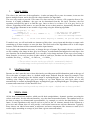
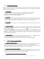
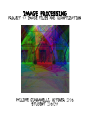
The original ‘Lena’ file
Out.setvalue(((int)In.getvalue(m,n)/constante)*constante,m,n);
rpt.addEventParamaterDescription("2^(B-A)","is made to divide and stretch. It is a constant.");
// description
rpt.addEventConclusion("We reduced the number of bits to encode the picture.\nIt can lead to false contours effects.");
}
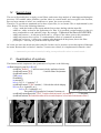
Using 1 bit (2 grey levels)
Philippe Giabbanelli
Using 2 bits (4 grey levels)
3
Using 3 bits (8 grey levels)
Images Files and Quantization
VI.
Experimentation
We also wanted to quantify the amounts of errors introduced by our quantization. For this goal, we
compute the relative error for each pixel, and we take the sum divided by the number of pixels. If the user
wants it, the relative error for each pixel can be saved ; because it slows the program, the option is off by
default. To implement this, we added some lines at the end of the function quantize :
file
FILE *exportFlot;
// export of the file in C mode (we apologize for that…)
if(img.exportCofiles()){
string exportFlotName = img.getOutputName() + "-ERROR.txt";
const char *c_str1 = exportFlotName.c_str ( );
if( (exportFlot=fopen(c_str1, "w")) == NULL){
cout << "!! Impossible to export error file. !!" << endl;
return;
}
fprintf(exportFlot,"---Error results for each pixel, in double precision---\n");
}
double taille = In.getwidth()*In.getheight(), erreurMoyenne(0.0), erreur(0.0);
// creating variable
for(int m = 0; m < In.getwidth(); m++){
// computing relative errors
for(int n = 0; n < In.getheight(); n++){
if(In.getvalue(n,m)!= 0) erreur = (double)abs(In.getvalue(n,m)-Out.getvalue(n,m))/In.getvalue(n,m);
else erreur = Out.getvalue(n,m);
core
erreurMoyenne += erreur;
// store the sum
if(img.exportCofiles()) fprintf(exportFlot,"%f ",erreur);
}
if(img.exportCofiles()) fprintf(exportFlot, "\n");
}
// we produce the report on this event. We remind the user about false contours effects if they are strong.
rpt.addEventConclusion("We reduced the number of bits to encode the picture.\nIt can lead to false contours effects.");
rpt.add("The average error is ");
rpt.add(erreurMoyenne);
rpt.add("/");
rpt.add(taille);
report rpt.add(" which is close to ");
rpt.add((100*erreurMoyenne)/taille);
rpt.add("%.\n");
if((100*erreurMoyenne)/taille > 6) rpt.add(" --> Warning, visible false contour effects ! <--\n");
if(img.exportCofiles()) fclose(exportFlot);
We also modified one line of the given algorithm :
“if lena256[m,n] = 0 then RelError[m,n] = |lena256[m,n] – lenaX[m,n]|”
Because lena256[m,n] = 0, this expression is simplified to RelError[m,n] = lenaX[m,n].
Of course, bigger is the ratio and stronger are the false contours. When we take Lena in 256 grey levels
and we turn in into 128 or 64 grey levels, the effects are not so easy to see. However, if we continue to
decrease the number of bits, then it leads to major problems, as seen in the previous page.
Philippe Giabbanelli
4
Images Files and Quantization
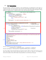
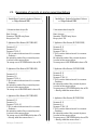
VII. Examples of reports on some experimentations
-------------------------------------------------------------| Detailed Report, Produced by Aqualonne's Software |
|
<c> Philippe Giabbanelli 2006
|
--------------------------------------------------------------
-------------------------------------------------------------| Detailed Report, Produced by Aqualonne's Software |
|
<c> Philippe Giabbanelli 2006
|
--------------------------------------------------------------
1. Informations about the input file
-----------------------------------Name : lena.pgm.
Dimensions : 250x250, using 1 layers.
Max grey level : 255.
1. Informations about the input file
-----------------------------------Name : tiger.pgm.
Dimensions : 250x250, using 1 layers.
Max grey level : 255.
2. Application of filter Quantize (10/17/06 11:49:12)
---------------------------------------Parameter B : 8
Parameter A : 7
Parameter 2^(B-A) : 2
2^(B-A) is made to divide and stretch. It is a constant.
---Conclusion--We reduced the number of bits to encode the picture.
It can lead to false contours effects.
The average error is 297/62500 which is close to 0%.
2. Application of filter Quantize (10/17/06 12:10:35)
---------------------------------------Parameter B : 8
Parameter A : 6
Parameter 2^(B-A) : 4
2^(B-A) is made to divide and stretch. It is a constant.
---Conclusion--We reduced the number of bits to encode the picture.
It can lead to false contours effects.
The average error is 1647/62500 which is close to 2%.
3. Application of filter Quantize (10/17/06 11:49:15)
---------------------------------------Parameter B : 8
Parameter A : 6
Parameter 2^(B-A) : 4
2^(B-A) is made to divide and stretch. It is a constant.
---Conclusion--We reduced the number of bits to encode the picture.
It can lead to false contours effects.
The average error is 884/62500 which is close to 1%.
3. Application of filter Quantize (10/17/06 12:10:38)
---------------------------------------Parameter B : 8
Parameter A : 5
Parameter 2^(B-A) : 8
2^(B-A) is made to divide and stretch. It is a constant.
---Conclusion--We reduced the number of bits to encode the picture.
It can lead to false contours effects.
The average error is 3779/62500 which is close to 6%.
--> Warning, visible false contour effects ! <--
4. Application of filter Quantize (10/17/06 11:49:18)
---------------------------------------Parameter B : 8
Parameter A : 4
Parameter 2^(B-A) : 16
2^(B-A) is made to divide and stretch. It is a constant.
---Conclusion--We reduced the number of bits to encode the picture.
It can lead to false contours effects.
The average error is 4440/62500 which is close to 7%.
--> Warning, visible false contour effects ! <-Philippe Giabbanelli
4. Application of filter Quantize (10/17/06 12:10:41)
---------------------------------------Parameter B : 8
Parameter A : 4
Parameter 2^(B-A) : 16
2^(B-A) is made to divide and stretch. It is a constant.
---Conclusion--We reduced the number of bits to encode the picture.
It can lead to false contours effects.
The average error is 7867/62500 which is close to 12%.
--> Warning, visible false contour effects ! <-5
Images Files and Quantization
VIII. A short user manual
Because a lot of things have been explained all along this paper, we don’t consider very useful to provide
a full manual. However, if the user wants to skip the technical aspect to focus on this use on the program,
then he can just read this section.
1) Open a picture
When the program starts, it asks for a picture of type PGM of PPM, in ASCII format.
Therefore, the user needs to give the name (and the path if necessary) of the file.
By example, if the file is in the same directory : lena.pgm.
If the file is in the root of C, then C:/lena.pgm
2) Apply a filter
Once the picture is opened, the user can apply the filter of his choice (now there is only one choice).
By example, if he wants to apply a quantization, he will write 1. Then, he will follow the instruction,
which are asking for some parameters and sometimes explain the effects of this parameter.
3) Save and quit
To save, we use s, and to quit we use q. A default filename is always provided, so the user doesn’t
need to write it.
4) Customize the output
It is possible to change the output parameters. If the user doesn’t like the default name provided by the
application, he can enter the one of his choice, by using n (like Name). He can also change the type of
the file, using t (like Type).
If the user wants to export the file related to algorithms (like the relative error), he needs to use c (like
Configure). Exporting this file slow the program, it is why we made such a choice. Then, the user can
turn on the export of related file. He can also decide to turn off the export of analysis, and then he
won’t be provided the full report.
5) Other major issues
If the user wants to see the comments included in the opened file, he can use v (as View comments).
A brief summarize of what have been done on the program is available by ?.
The output of histogram and the interactive analysis of a file are not yet implemented.
IX.
Things to do in next version
1) Converting from C style to C++
Because we are mostly a C programmer, we often used C functions, especially for saving the files.
We apologize for that, and we are currently taking the Advanced C++ Programming course.
When we will know how to deal with files and be sure of our memory management, we will turn the
C functions (fopen, fclose, fprintf, getc, malloc, calloc…) into C++ functions.
2) Trying to prevent erase of the original file
If the user wants to save his file with the same name that the original file, it will erase it. It is not a
problem for us, but we have to say the user that what he is doing can be dangerous, are you sure, etc.
We implemented a little function for this, which is not yet working.
3) Be sure that everything is also working on colours images
Philippe Giabbanelli
6
Images Files and Quantization