Download LIAR - A Computer Program for the Modeling and Simulation

:
I
SLAC/AP-103
April 1997
LIAR - A Computer Program for the Modeling and
Simulation of High Performance Linacs*
R. Assmann, C. Adolphsen, K. Bane, P. Emma,
T. Raubenheimer, R. Siemann, K. Thompson, F. Zimmermann
Stanford Linear Accelerator Center, Stanford University,
Stanford, California 94309 U.S.A.
Version 1.9 - April 1997
WWW-homepage
at
http://www.slac.stanford.edu/grp/arb/rwaAia~htm
_
*Work supported by Department
of Energy contract DE-AC03-76SF00.5
15.
DISCLAIMER
NOTICE
The items furnished herewith were developed under the sponsorship of the U.S. Government. Neither the
U.S., nor the U.S. DOE, nor the Leland Stanford Junior University, nor their employees, makes any warranty,~
express or implied, or assumes any liability or responsibility for accuracy, completeness or usefulness of any
information, apparatus, product or process disclosed, or represents that its use will not infringe privatelyowned rights. Mention of any product, its manufacturer, or suppliers shall not, nor is it intended to, imply
approval, disapproval, or fitness for any particular use. The U.S. and the University at all times retain the
right to use and disseminate the furnished items for any purpose whatsoever.
Notice 91 02 01
ABSTRACT
The computer program LIAR (“Linear Accelerator Research code”) is a numerical modeling and simulation
tool for high performance linacs. Amongst others, it addresses the needs of state-of-the-art linear colliders
where low emittance, high-intensity beams must be accelerated to energies in the 0.05-l TeV range. LIAR is
designed to be used for a variety of different projects. It has been applied to and checked against the existing
Stanford Linear Collider (SLC), the linacs of the proposed Next Linear Collider (NLC) and the proposed
Linac Coherent Light Source (LCLS) at SLAC.
LIAR allows the study of single- and multi-particle beam dynamics in linear accelerators. It calculates
emittance dilutions due to wakefield deflections, linear and non-linear dispersion and chromatic effects in
the presence of multiple accelerator imperfections. Both single-bunch and multi-bunch beams can be simulated. It is possible to simultaneously study the acceleration of positive and negative charges in a linac.
Diagnostic and correction devices include beam position monitors, RF pickups, dipole correctors, magnet
movers, beam-based feedbacks, multi-device knobs and emittance bumps. Several basic and advanced op- .
timization schemes are implemented.
Present limitations arise from the incomplete treatment of bending
magnets and sextupoles.
A major objective of the LIAR project is to provide an open programming platform for the accelerator
physics community.
We invite interested scientists to join this project. Due to its design, LIAR allows
straight-forward access to its internal FORTRAN data structures. The program can easily be extended and
its interactive command language ensures maximum ease of use. Presently, versions of LIAR are compiled
. for UNIX and MS Windows operating systems. An interface for the graphical visualization of results is
provided. Scientific graphs can be saved in the PS and EPS file formats. In addition a Mathematics interface
has been developed. LIAR now contains more than 40,000 lines of source code in more than 130 subroutines.
This- report describes the theoretical basis of the program, provides a reference for existing features and
explains how to add further commands. The LIAR home page and the ONLINE version of this manual can
be accessed under:
http://www.slac.stanford.edulgrplarb/rwaAiar.htm
:
1
Contents
1
1
CONTENTS
1
2
THE
2.1
2.2
2.3
5
5
5
6
3
4
5
_
--
Contents
LIAR PROJECT
..........................................
Cross-checks
..........................................
Compatibility
Updates, bug fixes and additional information
.........................
THEORY, CONCEPTS AND FEATURES
3.1 Phase space description .....................................
........................................
3.2 Beam description
.......................................
3.3 Beamline elements
3.4 Beam energy and Rf phases ...................................
.......................................
3.5 Optics calculations
3.6 Beam tracking ..........................................
3.7 Dipole wakefields ........................................
3.8 Quadrupole wakefields .....................................
3.9 Static imperfections .......................................
.....................................
3.10 Dynamic imperfections
3.11 Correction schemes .......................................
....................................
3.11.1 l-to-l correction
3.-l 1.2 Beam-based alignment and steering ..........................
3.11.3 Dispersion-free steering ................................
3.11.4 Other beam-based correction schemes .........................
3.11.5 Energy feedback ....................................
3.11.6 Position feedback ....................................
3.11.7 Global emittance bumps ................................
3.12 Observables ...........................................
............................................
3.13 Matching
3.14 Trajectory fit ..........................................
3.15 ~Diagnostic linac model .....................................
GETTING STARTED WITH LIAR
4.1 Setup ..............................................
4.2 Introduction to the command language .............................
4.3 Iterative command loops ....................................
- 4.4 Standard LIAR output ......................................
4.5 MATHEMATICA interface ...................................
4.6 Examples of SLC command files ................................
Simple SLC study ...................................
4.6.1
4.6.2
Advanced SLC study ..................................
LIAR COMMANDS IN THE SIMULATION CONTEXT
5.1 Initialization and setup . . . . . . . . . . . . . . . . . . . . . . . . . . . . . . . . . . . . .
5.2 Quitting the program . . . . . . . . . . . . . . . . . . . . . . . . . . . . . . . . . . . . . .
5.3 Maximum dimensional definitions . . . . . . . . . . . . . . . . . . . . . . . . . . . . . . .
7
7
7
8
9
9
10
10 .
11
12
12
12
12
13
14
17
17
17
18
19
21
21
21
24
24
25
27
28
30
30
30
32
36
36
36
36
2
Contents
5.4
5.5
5.6
5.7
5.8
5.9
5.10
5.11
5.12
5.13
5.14
5.15
5.16
5.17
5.18
5.19
6
Defining the lattice and the Rf .................................
........................................
Twiss calculation
Beam setup ...........................................
Wakefield setup .........................................
Accelerator imperfections ....................................
......................................
Trajectory feedbacks
Multi-device knobs .......................................
Tracking .............................................
Correction algorithms ......................................
Logbook .............................................
output ..............................................
Reference data .........................................
..................................
“Experimental” observables
Executing command files ....................................
Additional output files .....................................
............................................
Graphics.
COMMAND REFERENCE
SECTION
.......................................
.......
ATLMOVE
.......................................
AUTOPHASE ......
.......................................
.....
CALCTWISS
.......................................
.....
CALC-TWISSP
.......................................
...
CHECK--LATTICE
.......................................
.......
.CORRECT
.......................................
CORRECTP .......
.......................................
......
CLOSE-FILE
DEFINE-FEEDBACK
. .......................................
.......................................
DEFINE-MULTIKNOB
.. .......................................
DEFINE-SUPPORT.
.......................................
DFS ...........
.......................................
.....
DLUM-WAIST
.......................................
EMITC
.........
.......................................
......
EMITC-MKB
.......................................
......
EMITCDEF
.......................................
...
EMITCDEF-MKB
ERROR-GAUSSBPM
. .......................................
.......................................
ERROR-GAUSS-QUAD
.......................................
- ERROR-GAUSS-STRUC
.......................................
EXEC ..........
.......................................
EXIT
..........
.......................................
FDBK-GOLD ......
.......................................
.....
FDBK-MISAL
.......................................
.......
GNUPLOT
.......................................
LOAD ..........
.......................................
LOGBOOK .......
.......................................
MDLERR ........
.......................................
......
_ MEASBPM
--
36
37
37
37
37
38
38 :
38
38
39
39
40
40
40
40
40
42
42
42
43
43
43
44
44
44
45
45
46
46
46
47
47
48
49
50
50
51
51
51
52
52
52
52
53
53
54
Contents
MEAS_BUNCH
............................................
.........................................
MEASDISPERSION
MEASEMIT:
............................................
MEAS-PHASE
............................................
MEAS-PHASE2
...........................................
MEASJiEF
..............................................
............................................
MEAS-TRAIN
........................................
MISALIGN-SUPPORT
OPEN-FILE ..............................................
PLOT .................................................
...........................................
PRINT-LATTICE
PRINT_REF ..............................................
............................................
PRINT-TWISS
...........................................
PRINT-TWISSP
...............................................
QALIGN
QUIT .................................................
READ..
...............................................
READ-MAD
.............................................
READSLC
..............................................
.........................................
READSLC-ORBIT
.............................................
READ-TRNS
REFAVG..
.............................................
..
REF-SUB ...............................................
RESET
................................................
RFALIGN..
.............................................
RFSWITCHOFF
...........................................
..........................................
SCALELATTICE
SENS-YKICK .............................................
SENSYQUAD
............................................
SET_BEAM ..............................................
SET-BPMREF
............................................
SETCHARGE
............................................
...........................................
SET-CONTROL
..........................................
SET-CORRECTOR
SET_FEEDBACK ...........................................
.............................................
SETJNITIAL
..........................................
- SETMULTIKNOB
SET-RF ................................................
SET_LRWF_SA ............................................
SET-SR-WF ..............................................
SET-SRQ-WF .............................................
........................................
SET-.WF-TRANSV-LR
.........................................
SHOWDEFINITIONS
SHOW-FEEDBACK
.........................................
SHOW-MARKER
..........................................
.........................................
_ SHOW-MISALIGN.
--
3
55
56
57
58
59
60
61
61
61
62
66
66
66
66
67
67
68 .
68
68
69
69
69
69
70
70
70
71
71
71
72
73
73
73
73
74
74
75
75
76
76
76
77
78
78
78
78
Contents
4
........................................
SHOW-MULTIKNOB
..........................................
SHOW-SUPPORT
............................................
STOP .. ..!
TRACK ................................................
.............................................
TRACKC..
..............................................
TRACKCP
TRACKF
...............................................
..............................................
TRACKFC
TRAJFIT
...............................................
79
79
79
80
81
82
82
83
84
7
DO-IT-YOURSELF EXTENSIONS TO LIAR: THE INTERNAL DATA STRUCTURE
7.1 Understanding the command language .............................
7.2 Adding a command and subroutine ...............................
7.3 Accessing information from other parts of LIAR ........................
7.4 Dimensional constants and definitions .............................
7.5 Command parameters ......................................
.......................................
7.6 Control parameters
7.7 Physics constants ........................................
.......................................
7.8 Lattice description
........................................
7.9 Initial conditions
................................
7.10 Beam and wakefield description
.............................
7.11 Feedback loops and emittance bumps
7.12 Logbook data ..........................................
85
85
85
86
86
87
89 .
89
89
95
95
100
100
8
DESCRIPTION OF INPUT FILES
.......................................
8.1 Lattice description
8.2 Wakefields ............................................
Short-range transverse and longitudinal wakefields ..................
8.2.1
Accurate long-range transverse wakefields .......................
8.2.2
Simplified long-range transverse wakefields .......................
8.2.3
8.2.4
Long-range longitudinal wakefields ..........................
Arbitrary initial bunch distribution along z ......................
8.2.5
102
102
104
104
105
106
106
106
9
LIST OF PROGRAM
108
10 WHAT’S NEW
10.1 Version1.8
10.2 Version 1.9
SUBROUTINES
AND FUNCTIONS
112
. . . . . . . . . . . . . . . . . . . . . . . . . . . . . . . . . . . . . . . . . . . 112
. . . . . . . . . . . . . . . . . . . . . . . . . . . . . . . . . . . . . . . . . . . 112
11 KNOWN PROBLEMS
AND BUGS
113
12 ACKNOWLEDGEMENTS
13 REFERENCES
114
The LIAR project
5
2
THE LIAR PROJECT
The LIAR (“Linear Accelerator Research code”) project was started at SLAC in August 1995 in order to
provide a computing and simulation tool that addresses the needs of high performance linear accelerators.
Its first objective was to implement advanced simulations for the main linacs of SLC (50 GeV) and NLC
(500 GeV) at SLAC. Since then it has been applied to the LCLS project at SLAC (15 GeV), the CLIC project
at CERN and to studies of a possible future 2.5 TeV linac. The program can be applied to a broad range of
problems that vary widely in energy and beam parameters.
Interested scientists are explicitly invited to join the LIAR project and to contribute new features (commands). The LIAR code is put into the public domain and can be used and distributed freely. However, we
expect that publications that contain LIAR results make proper reference to this user’s guide. In addition we
ask that any extensions and modifications to this program are made available to the scientific community for
free usage. Contributions and questions should be submitted by e-mail to assmann @slac.stanford.edu.
2.1
Cross-checks
The name of this program does not indicate that all its results are wrong. Indeed, some effort was invested
to make sure that LIAR provides correct answers. LIAR results were cross-checked against the following
computer programs:
l
Transport [ 11.
l
LTrack [2].
l
Turtle -131.
l
Private codes from Raubenheimer,
Adolphsen
and Kubo [4].
The results show excellent consistency. In addition, SLC measurements were simulated with very good
,agreement. However, as always, there is no kind of warranty that results are correct. Bugs probably exist and
LIAR might occasionally “lie”. Problems should be reported by e-mail to assmann @slac.stanforcf.edu.
2.2
Compatibility
The LIAR code is mainly written in standard Fortran 77. It, however, takes advantage of the STRUCTURE
and RECORD extensions that are available in most Fortran compilers. The code is stand-alone apart from
a few system calls (random number generator, time) that need to be adjusted to the actual computer system.
No specific libraries are required for the compilation. LIAR version 1.9 is presently running under those
operating systems:
l
l
UNIX: (IBM AIX 3.2, etc.).
Computer: UNIX RISC workstations.
Windows 95 /Windows NT: (Personal Computers).
Computer: > Pentium 133 MHz, > 32 MB RAM.
Compiler: Microsoft Powerstation Fortran 4.0.
The code is easily ported, as long as Fortran compilers are available that support
RECORD extensions. A Macintosh version can be generated using the appropriate
Powerstation compiler. Unfortunately there is no free LINUX Fortran compiler
STRUCTURE’s and RECORD’s or Fortran 90 features. An adequate commercial
-available from Absoft (compare http://marie.mit.edu/
templon/fortran.html).
--
the STRUCTURE and
version of the Microsoft
available, that supports
compiler for LINUX is
.
6
The LIAR project
2.3
The most recent information
Updates, bug fixes and additional information
on LIAR is available through its home page on the World Wide Web
Please check for changes in the User’s Manual
information.
New versions of LIAR will be put to its AFS site:
or use the ONLINE
manual
with the most recent
/afs/slac.stanford.edw’public/so&vare/liar/release
Bug fixes will generally not result in a new version number. The existing version of LIAR will just
be updated. Every l-2 months, however, a new version will be released that contains all the old features
plus the new commands that have been added since the last release. If existing commands are enhanced
or significantly changed they will be available under a slightly changed name. The original commands
with their old functionality will be available under their old name. We thus will try to maintain backward .
compatibility.
Theory, concepts and features
3
7
THEORY, CONCEPTS
AND FEATURES
The overall design goal for LIAR was to provide a programming platform for simulations of linear accelerators. The basic structure was required to be flexible enough to include all beam physics and imperfections
that are relevant to the operation and optical design of linear accelerators. At the same time it had to be easy
enough to allow additions and extensions by non-experts. A working knowledge of FORTRAN should be
sufficient to join the LIAR project and to help supplying new features. An interactive command language
was implemented in order to ensure maximum ease of use. In the following we summarize the features and
basic concepts of LIAR version 1.9. In order to describe the charged particle beam transport we use the
TRANSPORT formalism [ 11. Modifications are mainly necessary to include wakefield effects and the beam
acceleration. LIAR profited from the experience with earlier simulation programs [4].
3.1
Phase space description
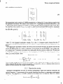
A position in phase space is defined by the 6-dimensional
vector
x
X’
xx
1J
where x < 0 is the head.
(1)
Y’
ri
L
The head of_the bunch is located in the negative x direction. Here, x and x’ are the horizontal displacement
and angle, y and y’ are the vertical displacement and angle, x is the longitudinal distance to the nominal
. center of the bunch and E is the total energy. Note that the definition of the energy coordinate differs from
the TRANSPORT convention.
The vector X describes the centroid motion of a thin longitudinal slice of a bunch. With each slice we can
,also associate a beam matrix 0. Since the bunch length is constant in linear accelerators, it is sufficient to
consider the beam matrix for the transverse planes only. It can be written as:
(2)
Here p, Q and y = (1 + (x2)//3 are the Twiss parameters, related by the Courant-Snyder
yx2 + 2cvxx’ + px12 = E
invariant:
(3)
This equation describes the beam ellipse which in a linear accelerator must be distinguished from the socalled machine ellipse (compare [5]). The lattice is designed for a given set of initial beam conditions.
This determines the design or machine ellipse (matched case). If the beam is injected with different initial
conditions then its Twiss values and the beam ellipse will be different (unmatched case). Even if the beam
is injected with the initial conditions matched, imperfections will generally cause the beam ellipse to differ
from the machine ellipse.
3.2
Beam description
The beam with a total charge of Q is described as a train of Nb bunches:
&=5&i
j=l
(4)
8
Theory, concepts and features
Each bunch is longitudinally divided into N, slices that are located at different positions x;. Note that Z; is
zero for the center of the bunch (without bending magnets) and negative for its head. PZ shall be the charge
distribution along Z-(it might be Gaussian) and its integral shall be one. IZ is a function of the bunch length
oz. The bunch charge Qj is distributed into N, slices at positions x; as follows:
N*
Qj = AL
i=l
. Qi
(5)
For a Gaussian distribution the slice positions xi are determined from the bunch length oZ, the number of
slices Ns and the number N, of standard deviations to be considered on each side:
xi=
(
i--
Ns + 1 .- 2Noaz
2 >
N.9
(6)
Finally each slice is divided into N, mono-energetic beam ellipses. IE shall be the energy distribution in a
slice. The function l?E depends on the uncorrelated energy spread oE. With DE, N,, and the number N, of
standard deviations to be considered on each side we obtain the energies E,,:
E,, =
and the corresponding
m -
Nm + 1 .
2
>
~N&E
NT’,,
(7)
charge distribution for each slice:
(8)
The beam description in version 1.9 is equidistant in slice position Z; along the whole accelerator. The next
version of LIAR will eliminate this requirement and will allow for changes of the bunch length in bending
magnets.
3.3
Beamline elements
Beamline elements that are defined in LIAR include
1. quadrupole
magnets,
2. dipole magnets (not complete in LIAR 1.9),
3. RF accelerating
structures,
4. beam position monitors (BPM’s),
5. horizontal and vertical dipole correctors and
6. marker points.
Dispersive effects are included for all elements. In a more general version of this program one would like to
include synchrotron radiation effects and sextupoles.
All elements are described as thick lenses. The transport matrices, R, that are used, are those defined in
the TRANSPORT formalism [ 11. They were modified only to include the transport through the preceding
drift space for each element. The beam is always tracked through the combination of an element plus its
preceding drift space. This allows to maximize computing speed. The transport matrix for each element is
--
Theory, concepts and features
9
calculated separately for each beam ellipse of each slice of each bunch (excluding drifts). Such all orders of
dispersion are included.
The accelerating RF structures are treated in a special way. They are described by at least two structure
pieces with an interleaved transverse wakefield deflection:
(9)
The matrix Rrf,2 transports the beam through one half of the structure. It takes into account the acceleration
and longitudinal beam loading. The matrix RWF describes the transverse wakefield deflections experienced
by each slice of the beam. Transverse wakefield kicks are thus lumped together into the middle of the
structures. This ansatz is refined by breaking up the structures into many pieces2. Each structure piece is
then treated with the ansatz shown above. Tracking through the RF structures involves convoluting the beam
with beam-excited transverse and longitudinal wakefields.
3.4
Beam energy and RF phases
A major problem in the operation and optimization of a linear accelerator is the choice and implementation
of the right phases between the beam and the accelerating RF. Adjustments in the RF phases allow for .
example the implementation of bunch compressors or BNS damping. Changing the RF phases will modify
the effective acceleration and the beam energy. It is necessary to readjust the beam energy to its design value
and to scale the quadrupole strengths accordingly. Longitudinal wakefields will cause further energy loss
that must be compensated in order to avoid a lattice mismatch. LIAR provides for a consistent way to adjust
the RF phases and the final beam energy. The energy loss SE from single-bunch longitudinal wakefields is
estimated in lattice calculations from
SE = -Kloss . Q . L
(10)
where Kloss is the loss factor (e.g. Kloss = 5.05 x 1014 V/C/m for NLC and Kloss = 6.6 x 1013 V/C/m for
SLC),-Q is the single bunch charge and L is the length of the RF structure3.
3.5
Optics calculations
The Twiss values of the “machine ellipse” are calculated under the following assumptions:
1. zeros bunch length
2. zero current
3. no transverse wakefield effects
However, longitudinal beam loading can be included with the simple analytical estimate from Eq. 10. The
“machine” Twiss values are purely determined from the transport matrices of the beamline elements. The
same matrices that are used for tracking, are used for the optics calculation. However, no particle tracking
is done. We call the result of this calculation the “design model”. This model is used for all correction
algorithms where the transport matrix between two points in the accelerator needs to be known. Due to
wakefields and imperfections, this model is only approximately correct. However, it is easily known and it
is sufficient for the accelerator operation, as long as correction schemes are iterated. In order to improve
21n order to divide a structure into pieces, the lattice input files do not need to be changed.
A command parameter in
READTRNS
and READMAD
allows to break a structure into a number of pieces from within LIAR.
‘The parameters for the short-range longitudinal wakefields are specified in the commands that make use of this simple approximation.
--
Theory, concepts and features
the convergence of correction methods, an improved “wakefield model” might be used. Serious correction
problems will most likely result from local errors in the quadrupole fields, the acceleration and the RF phases.
Those errors can be set in LIAR and can be included or excluded from the Twiss calculation.
3.6
Beam tracking
Beam ellipses are tracked fully coupled in 6D (without synchrotron
the beam ellipses o are tracked through the lattice:
radiation).
X1 = RX”
Both the centroids X and
(11)
and
o1 = Ra,,RT
(12)
The beam can be defined as a sequence of electron and positron bunches. The lattice is scaled internally
according to the sign of the bunch charge. Wakefields can be arbitrarily switched on and off for the tracking.
3.7
Dipole wakefields
Both single-bunch and multi-bunch dipole wakefield effects are included for the transverse plane. The
wakefields are read in as parameterizations from design specific input files (compare section 8.2). In the
transverse planes, imperfections of the long-range wakefields can be defined. As long as there are no imperfections, the transverse wakefield kick per unit offset per energy per charge is the same in all structures.
Long-rangewakefield
imperfections are defined for a small number of “imperfection types” that are ran. domly assigned to the RF structures. Long-range longitudinal wakefields can be represented as well.
A slice i experiences an energy loss 6E; due to short-range longitudinal wakefields that are excited by all
preceding slices j. It is determined as follows:
SE; =
q”(o)
2
i-l
1
I&i1+ c W,r”(i - j) +Qj . L
jZ1
(13)
Here the Q;,j are the charges in the slices i or j and W,,SR is the wakefield function as determined from the
design specific input file. The head of the bunch is i = 1 and the sum term is only evaluated for i > 1. L is
the length of the structure.
A slice I in a bunch Ic experiences a transverse trajectory deflection 19, due to short-range and long-range
wakefields that are excited by the preceding slices in all preceding bunches. The deflection angle is:
k-l
&(k,l)
=
CQjz,LIW,LR(I;-j,~,T,E)+~i.W~LR(k-j,~~T,E)]
(14)
j=l
l-l
+ c Q;x;LWfR(Z - i)
i=l
(15)
The Qj are the bunch charges and the Qi the slice charges. WiR(k - j, P7 T, E) is the long-range wakefield
function for the bunch “distance” (Ic - j . &~~,lncrl) , the structure piece P, the structure type T and the error
type E. WiLR(k - i, P:T, E) is its derivative with respect to the longitudinal offset ZEto the bunch center.
Long-range wakefields can be defined for different structure types T and different error types E. The term
JVTR(Z - i) specifies the short-range transverse wakefield function for a slice distance (I - i . Asslice).
11
Theory, concepts and features
3.8
Quadrupole wakefields
If a beam possesses a transverse quadrupole moment relative to the accelerator pipe axis, e.g., if the beam
is not round or off -axis, a quadrupole wake is generated. Although typically much weaker than the dipole
wake, the quadrupole wake may not always be neglected, since it is not easily recognized and its effect can
be orthogonal to that of the dipole wake. The implementation in LIAR closely follows the prescription by
Chao and Cooper [ 111.
Two types of quadrupole moments exist: a normal quadrupole moment Qq,i and a skew quadrupole moment
Q (],x,which are defined by
Q (111 =
Q (12 =
<x2>-<y2>
(16)
2<s’y>
(17)
The wake field generated by a slice with quadrupole moments Q,],i and Q,1,2gives rise to a Lorentz force on
another slice following a distance x behind it [ 111, which reads
e(,+;x,)
= e2W(4
[Q,,I
( x2 - y$) + Qq,2 (‘~2 + ~$1
(18) .
where W(z) is the quadrupole wake function, and i and 6 denote unit vectors in the horizontal and vertical
direction.
In LIAR only the short-range quadrupole wake field is implemented. For the lath slice, the transfer matrix
through a half
__ structure of (half) length L is given by [ 111
[l
R qwl
=
Ql
0
0
01
1
Y2
0
00
(19)
10
1 Q2 0
-9
1 J
where
” =$ kg
Niwz(x;
- x~)&,,~,;
2-l
(W
and
(21)
The sums are taken over all the previous slices, and Ni is the charge of slice i in units of e. The quadrupole
moments of the ith slice are
(22)
Qq,l,i = ozz,i - oyy,i + Xf - yf
and
Qq,2,i = 2ozy,i + 2xiyi
(23)
where the o’s denote elements of the sigma matrix for the ith slice. The quadrupole
SLAC linac was calculated by Bane and Wilson [ 11, 121:
W2(Ax) M 0.38 x iOl” m-:’ (Ax/l.5
The quadrupole
function.
--
wake function
for other accelerators
rr,rr,)“.cg3-o.10(n”1 Inm)
can be estimated
wake function for the
(24)
by scaling from the dipole wake
Theory, concepts and features
3.9
Static imperfections
Imperfections are understood to be static if their magnitudes do not significantly
scale. Here we give a list of error types that are presently implemented:
1. Quadrupoles: Transverse positions, rotation angle about longitudinal
change on an hourly time
direction (roll), strength.
2. BPM’s: Transverse positions, transverse positions with respect to quadrupole centers, finite resolution.
3. Accelerating structures: Transverse positions (offset misalignment),
misaligned on girders, as whole structures or in sub-pieces.
3.10
Dynamic imperfections
over minutes or hours.
gradient, RF phase. Structures are
Dynamic imperfections
are imperfections
which may change from pulse to pulse or may drift significantly
‘1.. Ground motion: Random ground motion (vibrations) and drifts as predicted from the ATL-model
a2=A.T.L
[9]:
(25)
where T is the time in seconds and L is the distance in meters, and A is a constant.
__
.
2. Timingjhctuations:
3. Initial conditions:
tion/intensity/phase
Random or systematic changes of the RF phase in the entire linac.
Random
jitter”).
and systematic changes of the initial beam parameters
3.11
(“incoming
posi-
Correction schemes
Emittance preservation in accelerators requires the application
we implemented a number of different methods.
3.11.1
l-to-l
of several correction
algorithms.
In LIAR
correction
Standard correction scheme with dipole correctors. Two choices are available:
,I. Least-square minimization of the BPM readings using dipole correctors over a range of the linac. The
l-to-l approach means that exactly one downstream BPM is assigned to every dipole corrector. The
number of BPM’s is equal to the number of dipole correctors. Usually only correctors at high p values
are used for trajectory correction. This means that the information of half of the BPM’s is not used in
the 1-to- 1 correction scheme.
For the least-square minimization the R i2 elements of the beam transfer matrices are needed. If the
dipole corrector is located at location ‘1 and the BPM at location 2 then the RI2 is calculated from the
Twiss parameters:
R12
=
e si+$)
(26)
.
Theory, concepts and features
13
where A$ is the phase advance between the two points, El and E2 are the beam energies and pi and
,82 the p-functions. We then solve for the dipole corrector strengths Ki in order to minimize all BPM
readings xj :
min
(27) :
R:,-‘2
R&+2
... ,T2+r,
The straight-forward Twiss calculation (compare above) does not include any wakefield effects. This
l-to-l optimization algorithm should therefore be iterated in small regions in order to converge to the
final solution.
2. Iterative minimization of each BPM reading by using one upstream dipole corrector (= 7r/2 upstream).
This is a fast approach that works well in simulation but cannot easily be realized in large accelerators.
3.11.2
Beam-based alignment and steering
Beam-based alignment of quadrupoles and accelerating
readings so that it also works as a steering algorithm.
structures.
This algorithm
minimizes
the BPM
The algorithm minimizes the quadrupole and structure BPM readings by first moving the quadrupoles,
thereby steering the trajectory, and then moving the accelerator structures to align them along the beam
trajectory. Because of imperfections in the accelerator model, a long linac is typically divided into many
shorter regions of 50 to 100 quadrupoles and the algorithm is applied to each region individually. To obtain
fullycorrection, one usually has to iterate the correction multiple times. The simulations include the effect of
‘finite BPM resolution (reading-to-reading jitter) and accelerator component misalignments.
The algorithm determines the quadrupole movements in an attempt to align the magnets in a straight line
between the first and last quadrupoles of the region being considered; the first and last quadrupoles of the
region are not moved by the algorithm. The beam is then launched along the beamline by adjusting either
the initial conditions, for the first region of the linac, or by adjusting a single dipole corrector located at the
first quadrupole for all subsequent regions; only a single dipole corrector is needed to join regions because
the beam trajectory should be centered at the first quadrupole which is the last quadrupole of the preceding
region. Finally, weights can be added for the BPM resolution and the quadrupole movements; the nominal
values are the expected BPM resolution and the expected quadrupole misalignments with respect to adjacent
magnets. These weights will limit the magnitude of the moves, constraining the trajectory to lie along the
pre-determined axis which can be assumed to be set by the initial mechanical alignment.
In specific, the quadrupole
alignment algorithm finds the least squares solution to the problem:
Y2
= RI
qN-1
Xl
x’1
1
or
Ri
(28)
:
I
14
Theory, concepts and features
with a weighting vector given by
(29)
The measurement vector consists of N BPM measurements mi followed by N zeros which are used to limit
the quadrupole movements. The solution vector consists of N - 2 quadrupole movements followed by x1 and
xi which are the initial conditions or 01 which is a corrector located at the first quadrupole of the region. Next,
the weighting vector consists of cb,,, oVU,Ld,and oinit which are the estimated BPM resolution, quadrupole
misalignments and initial error which nominally would be equal to the quadrupole misalignments.
Finally,
the matrix R is given by:
Rr =
0
0
...
0
%I
R21
-1
0
...
0
Rll
R21
K2R12
-1
...
0
&I
R21
...
0
Ru
R21
Ril
Ril
KzRl2
K3Rl2
(30)
. . .
K2k12
K3k12
...
K~-,h?l2
. where K; is the integrated quadrupole strength, R 12 is the (1,2) transport matrix element from the ith
quadrupole to the BPM, R11 and R2l are the (1,l) and (2,l) matrix elements from the initial point to the
BPM’ s.
After applying the quadrupole solution, the movers on the accelerator structures are adjusted such that the
average RF-BPM reading on a girder is minimized. Each structure has two RF BPM’s, one at either side.
Let’s assume that fi structures are mounted on a single girder that has a mover at either end. We then have
2 e fi RF BPM readings x; at the locations si with i running from 1 to a. We then obtain the girder to beam
offset Ax at every location s from
Ax(s) = me s + c
(31)
with
(32)
This is a simple straight line fit to the RF BPM readings. s and ; indicate the averages over all si and 5’;. In
order to align the RF structures, a mover at a location s,, is moved by -Ax( s,). Adjusting both movers on
a girder will thus minimize the average RF BPM reading.
3.1 I. 3
Dispersion-free steering
Quadrupole misalignments (but also RF structure misalignments) cause both trajectory deflections and
centroid dispersion. A measurement of the centroid dispersion then allows to compensate misalignments
effectively. The dispersion qZ in LIAR is defined as the change Ax(s) in trajectory offset for a relative
energy change A E/E:
AE
Ax(s) = ~z(s)~
= 7/z&$
.
(33)
:
I
Theory, concepts and features
15
In order to determine the dispersion, AEIE is assumed to be constant along s. Equivalent to changes in
the beam energy E is a change in the lattice strength K (for quadrupoles and correctors; transverse structure
deflections can be neglected). For practical reasons dispersion in linear accelerators is best measured with a
lattice scaling.
Note that dispersion in a linear accelerator is not as uniquely defined as in a storage ring. However, the
definition used here provides a dispersion that is a well defined observable. From the measured dispersion a
dispersion-minimized
trajectory can be calculated. This is called “Dispersion-free Steering” [ 131.
Since the superposition of many errors generates the dispersion, a model for how a deflection at any location
changes the trajectory at all downstream locations is required. Neglecting wakefield effects, the absolute
reading xj at a BPM j due to all upstream kicks 0; is
.i
=
j-1
c
R&+i
0; ,
(34)
i=l
from the kick i to the BPM j are given by
where the transport matrix elements Ri$
42
i-bj
_
-
(35)
Here the l&i are the beam energies, the @ are the beta functions and the tiii are the betatron phase
advances.
Now we Calculate how the dispersive kicks change the difference trajectory AxJ’ when the lattice is scaled
. (equivalent to change in beam energy). For the scaled lattice we need to recalculate the Twiss parameters
(primed quantities). Then obtain for Axi
j-1
Axi = .i - x’i = c
R”l;f 0; ,
(36)
i=l
where the R$i are the transport matrix elements for the scaled lattice. We define a lattice scaling factor TV
from the change AK in the quadrupole strength K as
AK
f$= -+1.
K
(37)
Effects from non-linear dispersion are neglected, since we use more than one lattice scalings for our analysis.
The dispersion-free solution should be local. Dispersion bumps are not easily possible and linear and nonlinear dispersion are minimized simultaneously. For a given lattice scaling K.the Rizi are
i-tj
R 12,rc -_
Ri;i
_
K
(38)
The Twiss parameters are calculated with the longitudinal magnet positions, the magnetic field values of the
quadrupoles and the beam energy at each magnet.
The above model predicts the effect of dispersive deflections on the absolute trajectory xi and the difference
trajectories AxJ’ (h). Alternatively, if we scale the lattice and measure xi and Axj (h) we can use the model
to calculate corrector settings that minimize both xi and Axj (K). With four sets of measurements in each
--
:
I
16
Theory, concepts and features
hysteresis cycle and n BPM’s we define the vector B of measurements
1
W1
ax?@)
2;:
ax2
B=
Ysl)
W&)
i;;;r
x
as
2
Wi(K3)
W2
(&I)
wa4
Ax2 (K~)
Ax2(rc3)
)
w=
wsd
(39)
waK3)
Tin
Q(Q)
W(K2)
WZ(K3)
with W as the vector of weights. The hi correspond to different lattice scale factors K. For each of the n
BPM’ s we have four measured quantities. The weights are defined through inverse measurement errors. Let’ s
first consider the absolute trajectory measurement xj. Its measurement error has a statistical contribution
The statistical
a(xj) M ares and a systematic contribution CJbpn-,from the absolute BPM misalignment.
error a(xj) arises mainly from the BPM resolution
. misalignments. The weight on xj is then
and is usually much smaller than the individual
BPM
(40)
Ideally the error on the measured trajectory difference Axj only has the statistical contributions
measurements. The weights on Ax3 are then defined by the BPM resolution ores
WQKj)
= $.
res
of the two
(41)
Equations 40 and 41 define the x2. The BPM resolution is usually much better than the BPM to quadrupole
alignment and we can write approximately
(42)
Therefore,
--
minimizing
the dispersion
makes optimum use of the BPM’s and is much more efficient than
Theory, concepts and features
solely minimizing
17
the absolute trajectory. We next define a correlation matrix
R:,t’
Rl+l
0
0
0
0
12,&l
Rl-bl
12,KQ
R2+2
12
R1+2
&2
12,&(.1
R1+2
12,nz
R1+2
(43)
1%‘~
RI’”
12
Rl+7L
12,K.l
Rlt7L
1242
R2trL
12
R2-f”
l&K1
R2’”
mw
R2-+7~
%W
and solve for the vector X of corrector settings:
The solution X provides a set of corrector strengths that minimizes the trajectory and dispersion measurements simultaneously. Instead of solving for corrector kicks we could have solved for quadrupole positions
that minimize the absolute trajectory and the dispersion.
3. Il.4
Other beam-based correction schemes
Wake-free steering algorithm (not yet fully implemented).
3. Il. 5
Energy feedback
Fix the energy at a location using dedicated feedback klystrons (not yet implemented).
The actual beam
energy E is adjusted to the energy setpoint ERetp. Note that we do not define any energy reference as for the
position feedbacks.
3.1 I .6
Position feedback
A generic implementation without worrying about technical feasibility is realized. A feedback is defined
by a reference position and angle
and
xLef
Gf
(45)
and the setpoints
and
xsetp
(46)
xbetp
at a point in the linac. Two upstream correctors that are reasonably close and efficient are used to adjust the
actual beam position and angle (zb,,,, XL,,,,,) to the reference values plus the setpoints:
5’beam
+
5’ref +
xwtp
(47)
&ml
-+
&f
Lkp
(48)
+
A feedback can be iterated in order to achieve the best agreement. In the LIAR implementation the ~1,~~~
and &mn at the feedback points are calculated with respect to the design plane. That is different from a
18
Theory, concepts and features
real implementation, where a number of BPM readings are used to fit xbeam and xLearn at one location in the
linac. An obvious problem occurs when the beamline has large, long wavelength misalignments.
A “real”
feedback would not see those kinds of misalignments since the whole beamline locally moves. However, in
LIAR the generic feedbacks would try to steer the beam back to the design plane which obviously is wrong.
A command is provided to “misalign” the feedback reference to the beamline (FDBK-MISAL).
This generic feedback definition is well suited to describe the feedback stabilization of slow drifts for times
larger than about 10 seconds. It is not suitable e.g. to study the pulse-to-pulse feedback response to fast
changes.
3.11.7
Global emittance bumps
A global emittance bump correction is implemented. Emittance bumps are trajectory oscillations that are
excited with a feedback at one point so and closed with another feedback at some other point ~1. The minimal
emittance using such a bump is obtained using a deterministic approach. Minimizing the emittance means
minimizing the Courant-Snyder invariant. We define a x2 at an observation point downstream of the two
feedbacks:
(49) .
with
2
05
=
E
~
Wi(Xi - ,Yi)2 -
i i=l
i=l
--
dz’
=
2
Wi(x; - 1J;)
2
Wi(Xi - yi)(x:‘; - y:) {
i=l
(50)
1
W;(X; - yi)
5
Ii
i=l
Wi(X’z
(51)
i=l
2
a;,
XI 5
Wi(Xi - y:)” -
2
Wi(X: - j/i)
1 i=l
i=l
(52)
1
The x; and x’; are the offset and divergence of every slice i before the application of the emittance bump. y;
and y: are the slice offsets/divergences
needed to minimize the emittance. The number of the slices in the
bunch is N,. The weights W; of the slices are defined as
w. = !i!i
’
Q
(53)
where Q is the total bunch charge and Q; is the charge of the slice.
The absolute minimum of the above x2 occurs when all the y;, y: are equal to the x;, xi. However, a single
emittance bump cannot provide enough degrees of freedom to actually achieve that. We express the slice
positions yi and divergences y: in terms of the setpoints x0 and xb for the first feedback:
yi
=
3: =
AixO + B;x~
(54)
CiXO +
(55)
DiX;
The coefficients A;, Bi, C; and Di are obtained experimentally by varying the setpoints ~0 and xb while
observing the y/; and y:.
Solving for the minimum x2 provides the following solution for the optimal setpoints:
opt
K
['opt,
1=H-l.
X0
X0
(56)
*
Theory, concepts and features
19
The vector K depends on the slice offsets and divergences at the observation point and is defined as follows:
K1
=
my C W;X;A; - C W;X; C W;A; + p
( i
i
1.
)
+a
K2
=
i
i
(57)
1.
C WixiCi + C Wix:Ai - C Wixi C WiCi - C WAX: C WiA;
i
i
i
i
1.
( i
)
7 CW;xiBi-CWixiCWiBi
( i
i
+a
C Wix:Ci - C Wix: C WiCi
(
(;
i
)
+/I
(58)
CW~X:D;-CW~Z:CW~D~
( i
i
i
)
CWix;Di+CW;z:Bi-CWix;CWiDi-CWix:CWiBi
i
i
i
(59)
(60)
i
i
)
The 2 x 2 matrix H depends only on the transfer coefficients Ai, Bi, Ci and D;:
Hll
=
T{TKAf+2o
H22
=
--
H12
=
{
=
(FiiBi)'}
C WiBiDi - C WiBi C WiD;
i
i
i i
+a
Ii
{
i
(61)
(62)
1
iD[TWDf-
7 CWiAiB;-CWiAiCWiBi
i
{ i
+p
(TWCi)2}
C WiAiCi - C WiAi C WiC;
y{TiiBf-
+2a
Hz1
(TWai)2}+:i{FKCf-
(63)
(TWDi)2}
(64)
1
(65)
1
% WiCiDi - C WiCi C WiD,
i
i
1
(66)
CWiBiCi-CWiBiCWiCi+CW;DiAi-CWiDiCW,Ai
i
i
i
(67)
i
i
i
From equation 56 we obtain the following explicit expressions for the optimal setpoints:
x wt
0
1
=
HllHm
‘opt
x0
-
H122
-
H122
(H22K
-
H12K2)
(68)
(f&K2
-
H12&)
(69)
1
=
HllH22
(70)
Due to limitations of the beam instrumentation, the slice offsets and divergences are not known individually
in a real accelerator. The bump setpoints are therefore optimized manually in order to minimize the measured
bunch emittance. However, future advances in the beam instrumentation could provide for a deterministic
emittance optimization like it is described here.
3.12
Observables
There are many relevant observables defined in LIAR. Obvious observables are the phase space positions
-at MARKERS (and part of it at BPM’s) for slices, whole bunches or the whole beam. Also obvious are the
--
.
:
I
20
Theory, concepts and features
“machine” Twiss parameters (/3, CX’,
ti . . . ) at all elements and for electrons and positrons.
beam emittance with respect to the beam centroid as:
We define the
where
(72)
1
?)” + Cz’z!,i
(74)
(75)
(76)
(77)
i=No
The sum runs over the individual beam ellipses in the beam. No and N can be chosen such that the emittance
. is calculated for the whole beam, a single bunch or a single slice. If the beam emittance is calculated, then
No is equal to 1 and N is equal to the product of the number of bunches, the number of slices per bunch and
the number of mono-energetic beam ellipses per slice:
Nt = Nb - N, . N,,,,,
(78)
Qi is the charge in the beam ellipse i and gzz,i, oZI2I,Zand gzz’,i are the beam ellipse parameters as introduced
in equation 2.
The emittance is not a measure of luminosity reduction. Large emittances often result from large tails that
contain only little charge. A figure of merit for luminosity reduction can be obtained from a cross-correlation
of a bunch with itself. Beam tails are naturally de-weighted. We define the following luminosity reduction
factor R:
(79)
The double sum runs over all slices in a bunch. The G are the average centroid offsets of the slices and the
ai,j are the RMS sizes of the given slice. Note that this definition of the luminosity reduction factor oscillates.
The final value obtained in LIAR is therefore averaged over the last 5% of the BPM’s in the linac.
The mismatch Pmag between the machine ellipse and the beam ellipse is of great importance in linear
accelerators. We use the following definition:
Here, Q and ,~3are the machine and o* and p* are the beam Twiss values. In the ideal matched case PIrlag is
-equal to one.
21
Theory, concepts and features
3.13
Optical matching routines are not implemented
3.14
Matching
at this time.
Trajectory fit
It is often necessary to fit the beam centroid offset and angle at some location “0” from a number “n” of
downstream BPM measurements. This fit has a unique solution and (x(O), x’(0)) can be calculated analyti- ’
tally as:
x(0)
=
C;;l R12(i) . x(i)
_ [C;zl R:,(i)]
C;;, &I (i> - &2(i)
x’(0)
=
XI”1 Rll(i)
. [CTzl R&)
. x(i)]
,
[IX:;“=1
RII(@~(~)]~
I
. x(i) - [C;zL=lR;,(i)] . x(0)
(81)
(83)
[C:zl Rll (+~z(‘i)]~
The fit naturally requires the knowledge of the R-matrix from the point to be fitted to all downstream
locations and the BPM readings x(i). This fit is implemented in the command TRAJFIT.
3.15
BPM
Diagnostic linac model
The transfer matrices in a linac can be very different from the ones that are calculated in a single-particle
model within LIAR. Reasons for this can be wakefield effects that are expected from the design (multiparticle beam dynamics) or errors in the beam energy, quadrupole strengths, etc. Analytical estimates for
. multi-particle beam behavior generally do not have the accuracy as required for the characterization of wakefield dominated linacs. In addition, parameter errors are by definition unknown in real accelerators. LIAR
therefore implements beam diagnostic observables that are determined from “measured” BPM values. The
same diagnostic method was applied for SLC very successfully. It allows to experimentally determine the
“real” linac optics. We follow the method that was first described in [ 141.
The linac beam transport is best described by the R-matrices for the centroid motion. As an example, let’s
define the linac R12,1’s. They can be written in a general form for locations “0” and “i” as:
This is a simple extension of Eq. 26 that was defined for design values without wakefields. The additional
factor ~2 describes any blowup of an induced linac betatron oscillation (for example due to head to tail
wakefield amplification).
Without wakefields and errors ~1 is exactly one. Note that the centroid phase
advance A$+ between two points in the linac can be strongly modified by wakefields, as well as the centroid
/%nctions.
The centroid beam transport in a linac can be described by examining the betatron oscillations (xi, xi) and
(22: xl) due to two beam deflections that are about 7r apart in phase advance (indicated by the subscripts 1
and 2). The R-matrix from an initial point number “0” (close to the origin of the beam deflections) to a
downstream location number “i” is obtained from solving simultaneously:
.
:
I
22
Theory, concepts and features
The result is:
Rll
=
R12
=
R21
=
R22
=
Xl(i) * xi(O) - x2(i) * xi(O)
x,(O) * x’,(O) - x2(0) - xi(O)
Xl(O) * x2(i) - Xl(i) * x2(0)
Xl(O)
* x;(o)
- x40)
* x’,(O)
xi(i) * x;(o) - x;(i) * x’,(O)
Xl(O)
* x;(o)
- x40)
* xi(O)
x;(i) * x,(O) - xi(i) * x2(0)
Xl(O)
* XL(O) - x2(0) * xi(O)
(87)
G33)
(89)
(90)
(91)
The R-matrix is then transformed
into normalized coordinates:
(92)
(93)
%l
--
=
o!
$Rll-
=R12
m
+
@ii%,,
-
CYO
RL2 =
(94)
(95)
This transformation requires the knowledge of the optical functions Q and /3 along the linac. Assuming that
they are locally correct we use the design Twiss values from the single particle model.
Now we can define a number of observables that describe the “real” linac optics4:
1. Centroid linac phase advance $1:
$4 = arctan
2. Enhancement
(96)
$
(
11 )
~1 of linac oscillation amplitude:
(97)
3. Linac p-function:
pl = (61
+ 5W2
.p
det RI
where c and s are defined as:
c = cos [arctan (g)]
_
and
s = sin [arctan ($)]
4Note that though we write the “arctan” function the “arctan2” function is used for the LIAR implementation.
(98)
Theory, concepts andfeatures
23
4. Linac a-function:
al =
(cR’,, + &)
(c&l + s&,)
det R’
+ “a
P
(1W
where c and s are defined as above.
5. The linac Pmaa mismatch is obtained with Equation 80, the linac optical functions
design optical functions /? and a.
,!31and QI and the
In order to describe a wakefield dominated linac completely, the two beam deflections must be induced along
the whole length of the linac, resulting in a two-dimensional table of R12’s. In LIAR we have implemented
the simulation and analysis of two incoming betatron oscillations as obtained from a possible diagnostic
pulse (see command MEAS-PHASE2).
24
Getting started
4
GETTING STARTED WITH LIAR
This section provides a basic introduction to LIAR. First we explain how to set up the program. Then we
describe the basic rules of the LIAR command language and the possibility of automatic command loops.
The standard LIAR output is explained and we provide two examples of both simple and advanced SLC
simulations.
4.1
Setup
LIAR is presently implemented for UNIX and MS windows operating systems.
located in a SLAC AFS account under UNIX. The released version is world-readable
Its home directory
and is located at:
is
/afs/slac.stanford.edu/publicIsoftware/liar/release
The directory tree is as follows:
. . . /bin.aix6000
. . ./examples
. . ./dot
Example command files.
Documentation
. . ./infiles
. . ./run
Executable for the IBM AIX unix system.
in LaTex and Postscript format.
Required input files (lattices,...).
Directory to run command examples.
. . ./src-vl.9
Source code for LIAR version 1.9 (including Makefile).
SLAC. workstations that are suitable for running LIAR include the SCS public machines morganol to morgan06. The liar directory tree.can be copied to a private UNIX machine and recompiled using the Makefile
which is provided. A VAX-VMS version is foreseen but is not yet compiled (volunteers are welcome).
In order to run LIAR as a SLAC user, get your personal UNIX account and e.g. login on morganol. Then
you could proceed:
1. Copy directory tree
' cP -r -p /afs/slac.stanford.edu/public/software/liar/release
2. Change to run directory
> cd liar/run
3. Copy example command file
> cp
. ./examples/cmdslcl
.
4. Run LIAR and execute command file...
> liar
cmdslcl
liar
Getting started
25
5 . . . . or execute LIAR in interactive mode
> liar
The Windows 95 PC version of LIAR runs as a console application in a DOS window.
LIAR can be run in two different modes. If it is started from the command level without any parameters
(e.g. liar) then it will enter into an interactive mode and the user is prompted for input:
III
III
III
--III
III
III
III
/II
IIIIIII
L I near
-IllIll
III
II
III-IIIIIIIIII
A ccelerator
SLAC
1997
---
T/I”
III
III
Version
R esearch
1.9
code
Ralph Assmann
Karl Bane
Tor Raubenheimer
Kathy Thompson
LIAR>
By typing the command
LIAR>
load,
file='cmdfile'
the command file cmdfile would be executed from the interactive program level. After all commands in the
.file have been executed the control is returned to the user who could now submit a few final commands to
complete the job. The interactive mode is used best for small simulations or for making sure that a bigger job
will provide useful results. The load command can only be used from the interactive level of LIAR. Nesting
of command files is not allowed.
LIAR automatically enters into a batch mode if it is started with a command file parameter. The UNIX
command
> liar
cmdfile
will start the program liar with the command file cmdfile as input. After all commands have been executed
LIAR is stopped. The batch mode is highly recommended for large simulation jobs. Since LIAR uses about
35 MBytes of random access memory the use of system resources is minimized by running in batch mode.
4.2
Introduction
to the command language
The LIAR command language is inspired from the MAD style [6]. However, our implementation is significantly different, allowing several flexible extensions. At the same time some restrictions are introduced.
Certain rules must be followed for the command line syntax. All those rules apply to both the interactive and
the batch mode of LIAR.
1. A command line (that can extend over several lines) consists of a command name and any number of
command options:
--
-
26
Getting started
LIAR>
track,
order=l,
command
option
couple
= .f.
option
Command options can be specified in any order and many of them can be omitted. Parameters that are
omitted use their default values. LIAR is not case sensitive5.
2. All parts of the command line must be separated by commatu. Spaces in the command line are ignored.
3. An input line that is ended by a comma is automatically
ended by breaking a line without a comma.
LIAR>
track,
The underscore
order
couple
continued
into the next line. A command
is
= 1,
= .f.
’ -’ is added automatically
by the command line parser.
4. Command options consist of the option name and its value. The values are assigned with an equal sign.
- It is essential that the values are specified in the following way:
(a) Logicals are specified by .t., .T., .f. or .F. (e.g. “couple=.t.“)! If a parameter is specified without an
equal (’ =’ ) sign, then it is assumed to be of type logical and to have the value .T.! So specifying
“couple” is equivalent to “couple=.t.“.
(b) Character strings must be enclosed in SINGLE quotes (e.g., file = ‘run/TEST’).
filenames are case sensitive, though LIAR is not.
Note that UNIX
(c) Every parameter that is not recognized as a logical variable or a character string and that contains
an equal (’ =’ ) sign, is read in as a REAL value. Therefore failing to obey to the rules described
will result in errors.
5. Each input line can take a maximum
input lines (9 continuation lines).
6. Comments
of 80 characters.
A single command
is allowed to take up to 10
are indicated by ’ !’ . Everything which follows on the particular input line is disregarded.
7. The use of TAB’s is not allowed. It will result in errors.
This is an example of a valid command line syntax:
ERROR-GAUSS-QUAD,
X-SIGMA
=
5.E-06,
Y-SIGMA
=
7.E-06,
T-SIGMA
=
1.E-06,
NAME
Lines of comments
fail:
X-SIGMA
=
5.E-06,
=
l.E-06,
Y-SIGMA.=
T-SIGMA
NAME
_
‘Q02*’
comment
comment
comment
comment
within the scope of a single command are not allowed. The following command
ERROR-GAUSS-QUAD,
I
=
!
!
!
!
=
7.E-06,
‘QO2*’
“However, keep in mind that UNIX filenames are case sensitive!
! comment
! comment
! comment
! comment
(WRONG)
would
:
I
Getting started
27
4.3
Iterative command loops
An advanced feature of the LIAR command language is the possibility to specify iterative loops over groups
of commands. Up to three nested levels of do loops are allowed. For each loop a step variable is defined that
can be used to specify command options. The basic do loop is implemented in a FORTRAN fashion:
DO SDY = lE-6,
lOE-6,
10
. . .
ERROR-GAUSS-QUAD,
X-SIGMA = 5.E-06,
Y-SIGMA = QSDY,
T-SIGMA = l.E-06,
NAME = 'QO2*'
!
!
!
!
comment
comment
comment
comment
. . .
END DO
In this example the variable SDY is stepped up from 1 x lo-” to 10 x lo-” in 10 steps. In the misalignment
command its value is accessed by @SDY. The implementation of do loops allows also to vary the seed of
misalignments or to modify filenames for the output (e.g. FILE=‘output@SEED’).
Using DO variables for .
outlz%itfilenames will only take into account the integer part of the variable (the allowable range is 0 to 1000).
Do loops are only permitted in input command files (executed with the commands LOAD, EXEC or
READ). They cannot be specified at the LIAR prompt. Do loops are expanded during a special preprocessing of an input file (e.g. ’input.liar’). If anything goes wrong the expanded input files (e.g. ’ input.liar-1 ’ ,
’ input.liar-2 ’ and ’input.liar-3 ’ ) can be found in the actual directory and should be checked for errors. The
expanded file .with the highest number will be actually executed. It should not contain any ’DO’ or ’ENDDO’
. commands!
--
:
I
28
Getting started
4.4
Standard LIAR output
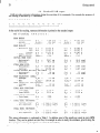
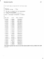
LIAR provides extensive information during the execution of its commands.
the tracking is indicated by a “trackometer”:
For example the progress of
TRACKOMETER:
0
10
20
30
40
50
60
70
l-l-l-l-l-l-l-l-l-l-l
________n_h_n_hh___h_n___nh___hhh
At the end of the tracking, summary information
End of tracking
80
90
100 %
is printed to the standard output:
ANALYSIS:
BEAM ENERGY
- acceleration:
E-0
=
1.190
- spread:
E-sig =
.016
- rel. spread
SIGE/E =
1.322
BEAM BLOW-UP
- Emittance
(bl):
31.621
g-x
=
(av):
31.621
g-x
=
(train):
31.621
g-x
=
- Lumin. factor:
R-x
=
94.6
- BMAG mismatch:
BMAGX =
1.030
INITIAL BEAM SIZE:
- Horizontal:
s-x
=
274.7
- Vertical:
sy
=
85.5
FINAL BEAM SIZE:
- Horizontal:
s-x
= 129.028
- Vertical:
s-y
=
45.858
JITTER OFFSETS WRT AXIS FOR BUNCH
0:
- Horizontal:
J-x
=
.94
JJ
=
- Vertical:
2.11
BEAM TRAJECTORY
(IDEAL)
X-av
=
- average:
-.lO
X-sig =
- RMS:
159.54
BEAM TRAJECTORY
(BPM READINGS)
X-av
=
- average:
.02
- RMS:
X-sig =
150.00
FINAL BETA FUNCTIONS
- from beam:
B-x
=
27.64
B-x
=
- from TWISS:
22.13
FINAL ALPHA FUNCTIONS
- from beam:
A-x
=
.7404
A-x
=
- from TWISS:
.7051
FINAL GEOM. EMITTANCE
- initial value:
= 1.293-08
E-x
- wrt centroid:
= 4.393-10
E-x
- wrt axis:
= 1.683-09
E-x
FINAL NORM. EMITTANCE
- initial value:
= 3.00E-05
E-x
- wrt centroid:
= 3.953-05
E-x
- wrt axis:
=.1.523-04
E-x
-->
-->
-->
E-f
E-sig
SIGE/E
=
=
=
46.003 GeV
.124 GeV
.269 %
%
%
%
%
gY
9-Y
KY
Ry
BMAGY
=
=
=
=
=
41.845
41.845
41.845
95.1
1.212
um
um
S-x'
S-y'
=
=
um
um
S-x'
SJ'
=
=
um
um
J-x'
Jy'
=
=
um
urn
Y-av
Y-sig
=
=
1.93 urn
113.64 urn
urn
um
Y-av
Y-sig
=
=
-3.67
110.48
m
m
B-y
BJ
=
=
51.34
27.25
Ay
A_y
=
=
-1.403
-.700
rad*m
rad*m
rad*m
KY
KY
EJ
= 1.50E-09
= 5.5lE-11
= 2.833-10
rad*m
rad*m
rad*m
rad*m
rad*m
rad*m
LY
E-Y
EJ
= 3.503-06
= 4.963-06
= 2.553-05
rad*m
rad*m
rad*m
GeV
GeV
%
%
%
%
%
64.6 urad
24.0 urad
3.685
1.247
urad
urad
-22 urad
1.12 urad
um
um
m
m
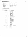
This output information is explained in Table I. In addition most of the results are saved at every BPM
location. They can be printed out into files, for example in order to study the emittance growth along the
linac (compare summary descriptions in sections 5.13 and 5.14).
--
:
Getting started
29
Headline
Beam energy
Label
E-O
E-f
E-sig
SIGE/E
Beam blow-up
g-x, g-y (bl)
g-h g-y (4
g-x, g-y (train)
R-x, R-y
Initial beam size
Final beam size
Jitter offsets
-Beam trajectory (ideal)
BMAGX, BMAGY
s-x, s-y
S-x’ ) S-y’
s-x, s-y
S-x’ ) S-y’
J-x, J-y
X-av, Y-av
X-sig, Y-sig
Beam trajectory (BPM)
X-av, Y-av
X-sig, Y-sig
Final beta functions
B-x, B-y
Final alpha functions
A-x, A-y
Geometric emittance
E-x, E-y
Normalized
E-x, E-y
emittance
Description
Initial beam energy in GeV
Final beam energy in GeV.
Absolute energy spread in GeV (start and
end).
Relative energy spread in % (start and
end).
X, Y emittance growth AC/CO of the first
bunch.
Average single bunch X, Y emittance
growth AC/Q.
X, Y emittance growth AC/C” for bunch
train (incl. bunch offsets).
X, Y luminosity estimate in % of ideal luminosity.
X, Y beta mismatch (1 = no mismatch).
Initial X, Y lo beam sizes.
Initial X, Y la beam divergence.
Final X, Y la beam sizes.
Final X, Y la beam divergence.
Beam offsets with respect to the axis or a
reference.
Average X, Y beam offset at BPM locations with respect to ideal reference line.
RMS X, Y beam offset at BPM locations
with respect to ideal reference line.
Average X, Y beam offset with respect to
BPM centers.
RMS X, Y beam offset with respect to
BPM centers.
X and Y beta function at the end of the
machine from (a) tracked beam and (b)
lattice Twiss calculation.
X and Y alpha function at the end of the
machine from (a) tracked beam and (b)
lattice Twiss calculation.
Geometric emittances at start and end of
tracking.
The final emittance is specified both with respect to the beam centroid and with respect to the ideal reference line.
Normalized emittances at start and end
of tracking. The final emittance is specified both with respect to the beam centroid and with respect to the ideal reference line.
Table I: Definition of quantities that are printed out as the summary information
after each tracking in LIAR.
Getting started
4.5
MATHEMATICA
interface
LIAR has been run within the MATHEMATICA environment. The interface allows to edit LIAR input
files, run the program and to process the LIAR output files all within the MATHEMATICA environment. The
mathematical power of MATHEMATICA can be very helpful in testing advanced optimization algorithms
or in comparing analytical theories with simulation results.
The MATHEMATICA interface consists primarily in a number of functions that transfer LIAR information
into MATHEMATICA objects and often also allow to plot them easily. Further information can be obtained
from Gennadi Stupakov at SLAC (e-mail: [email protected]).
4.6
Examples of SLC command files
We show two examples for SLC simulations. A simple SLC case allows the new user to get familiar with the
concept of the LIAR command language and the basic philosophy in setting up a simulation. An advanced
simulation demonstrates the capabilities of the computer program in defining multiple imperfections and
advanced correction schemes.
4.6.1
Simple SLC study
The first example considers a simple case where we just simulate the effect of an injection offset of 200 ,~rn
in both planes. It includes wakefield and dispersion effects and a setup for BNS damping. The trajectories
and emittances are calculated. The input file can be found in
. The listed commands
LOAD,
FILE
can be entered interactively or read in as a command file by specifying
= 'filename'
at the LIAR prompt (alternatively the READ or EXEC commands can be used). Note that exclamation
marks (’ !‘) indicate comments. In this example the command names are printed in upper case, all options
in lower case. Note however that LIAR is not case sensitive (though UNIX file names are). We first show
the complete command input file. We then will go through the details of the command file, explaining every
step.
RESET,
all
READ-TRNS,
SET-RF,
infile
energy
npiece
energy
scale
kloss
charge
phase1
lswitchl
phase2
CALC-TWISS,
= '../infiles/slc.trns',
= 1.19,
= 1
=
=
=
=
=
=
=
betax
betay
alphax
alphay
46.,
.t.,
0.66d14,
3.5d10,
22.,
800.,
-16.5
=
=
=
=
3.40,
3.08,
0.156,
0.066
-
Getting started
31
SET-INITIAL,
x
=
=
=
=
=
=
Y
energy
&spread
nemitx
nemity
match
SET-BEAM,
current
blength
nb
ns
nm
SET-SR-WF,
200.d-6,
200.d-6
1.19,
0.014,
3.d-5,
0.35d-5,
= 3.5d10,
= llOO.d-6,
= 1,
= 20,
= 3
file
=
'.. /infiles/srwf-slc.dat'
TRACK
MEAS-BPM,
file
=
'bpm.dat'
Now we step through this input file and explain the commands and their options. Note that we do only
specify the necessary options. Many more options exist, but we use their default values.
In the first simulation step all data areas are initialized to zero:
RESET,
all
Now we read in an SLC transport deck, define the injection energy and tell LIAR to treat each structure in a
. single piece:
READ-TRNS,
infile
energy
npiece
= '../infiles/slc.trns',
= 1.19,
= 1
The RF is set up with the command SET-RF. We specify the final beam energy (’ energy’ ), a first RF-phase
(’ phasel’ ), a switching point (‘lswitchl’ ) for the RF-phase at 800 m and a second RF-phase. The lattice and
the acceleration is scaled (‘scale’) to fit those RF-phases and the final beam energy. We also compensate for
longitudinal beam loading with a simple model (’ kloss’ and ’charge’ ).
SET-RF,
energy
scale
kloss
charge
phase1
lswitchl
phase2
=
=
=
=
=
=
=
46.,
.t.,
0.66d14,
3.5d10,
22.,
800.,
-16.5
It is always a good idea to calculate the Twiss values at all elements, though not needed for our example. The
initial Twiss values must be specified:
CALC-TWISS,
betax
betay
alphax
alphay
=
=
=
=
3.40,
3.08,
0.156,
0.066
:
I
32
Getting starred
We specify the injection energy, the initial energy spread and the initial normalized emittances. The ‘match’
option tells LIAR to match the beam to the Twiss values that were specified before6. We also define an
horizontal and vertical injection offset of 200 ,um (’ x’ and ’ y’ ):
SET-INITIAL,
x
=
=
=
=
=
=
Y
energy
espread
nemitx
nemity
match
200.d-6,
200.d-6
1.19,
0.014,
3.d-5,
0.35d-5,
Next we define the bunch population, the bunch length, the number of bunches (‘nb’), the number of slices
per bunch (’ ns’ ) and the number of mono-energetic beam ellipses per slice (’ nm’ ):
SET-BEAM,
current
blength
nb
ns
nm
=
=
=
=
=
3.5d10,
llOO.d-6,
1,
20,
3
Finally we specify the wakefields. The wakefield functions are read in as tables from input files, that have
been generated with specialized programs (e.g. with MAFIA [7] or [S]):
.~ SET-SR-WF,
Everything
file
= '../infiles/srwf-slc.dat'
is now set up to track the beam through the lattice:
TRACK
The end-of-tracking analysis prints a lot of useful data to standard output (e.g. emittance growth, RMS
trajectory offsets). Compare the example in section 4.4! In order to study details along the linac, we generate
an ASCII table that contains the BPM readings, the emittances, the beta mismatch and other observables as
a function of longitudinal position.
MEAS-BPM,
file = 'bpm.dat'
An external plotting program (e.g. gnuplot or PAW) can now read the ASCII table and generate plots. The
table format is described in the reference description of the command MEAS-BPM. Alternatively plots can
be generated directly with the command PLOT.
4.6.2
Advanced SLC study
Now we show an example of an advanced SLC simulation.
The input file can be found in
This example includes imperfections, BNS damping, trajectory corrections, feedback loops and emittance
The calculations are performed for 100 statistically different cases. This example
bump optimizations.
illustrates the power of LIAR to study imperfections and their correction.
- 6Alternatively
initial
beta
and alpha functions can be specified
Getting started
33
RESET, all
SET-CONTROL,
READ-TRNS,
SET-RF,
debug
outlun
dutfile
infile
energy
npiece
energy
scale
kloss
charge
phase1
lswitchl
phase2
CALC-TWISS,
! * Reset data
! * Send standard output
I
to file 'test.txt' on
!
unit 46.
= '../infiles/slc.trns',
= 1.19,
= 1
! * Read transport
input
!
deck and define injection
!
energy.
46.,
.t.,
0.66d14,
3.5d10,
22.,
800.,
-16.5
! * Set final beam energy
I
and RF phases. Scale
I
lattice accordingly.
betax
betay
alphax
alphay
SET-INITIAL,
--
=
=
=
=
=
=
=
= 0,
= 46,
= 'test.txt'
=
=
=
=
energy
espread
nemitx
nemity
match
I
3.40,
3.08,
0.156,
0.066
! * Calculate Twiss values.
!
Specify initial beta
!
and alpha functions.
!
=
=
=
=
! * Specify initial energy,
I
energy spread, normalized
I
emittances.
Match initial
I
beta and alpha to Twiss.
1.19,
0.014,
3.d-5,
0.35d-5,
I
SET-BEAM,
SET-SR-WF,
current
blength
nb
ns
nm
file
= 3.5d10,
= llOO.d-6,
= 1,
= 20,
= 3
! * Set up beam. Specify
I
bunch population,
bunch
I
length, number of
!
bunches/slices/macro!
particles.
=
! * Define
' ../infiles/srwf-slc.dat'
short-range
WF's
!
DEFINE-FEEDBACK,
DEFINE-FEEDBACK,
DEFINE-FEEDBACK,
marker
marker
marker
= 'feedbk06'
= 'feedbkll'
= 'feedbkl8'
TRACK
! * Define feedbacks at
I
predefined
markers.
I
! * Track
beam
through.
!
EMITC-DEF,
name
fdbk
wire
iter
cars
xfile
yfile
titer
= 'ebumpl',
= 'feedbk06',
= 'wireOOOl',
= 8,
= 'sic',
= I.. /infiles/xmatch.ext-elec',
= I.. /infiles/ymatch.ext-elec',
= 1, silent
EMITC-DEF,
name = 'ebump2',
fdbk = 'feedbkll',
wire = 'wire0002',
iter = 6,
cars = 'sic',
! * Define emittance bump
I
using the feedback
!
'feedbk06' to minimize
the emittance at a
!
I
predefined
marker.
Calibrate bumps using
!
!
l-to-l correction
(SLC
scheme).
!
!
! * Define
!
bump.
!
!
second
emittance
:
r--~
34
Getting started
xfile
yfile
titer
= I.. /infiles/xmatch.ext-elec',
= I.. /infiles/ymatch.ext-elec',
= 1, silent
LOGBOOK, reset
RESET, reference
DO seed
= 1, 100,
! * Reset
! * Reset
! * Do 100 different
100
RESET, corrector
LOGBOOK, set = 1
ERROR-GAUSS-STRUC,
ERROR-GAUSS-QUAD,
ERROR-GAUSS-BPM,
TRACKC,
_-
_
the logbook.
reference data.
! * Reset corrector
! * Specify logbook
name
= '*I,
x-sigma = 200.e-6,
y-sigma = 200.e-6
name
= I*',
x-sigma = lOO.e-6,
y-sigma = lOO.e-6,
bpm
= .t.
name
= '*I,
x-sigma = lOO.e-6,
y-sigma = lOO.e-6,
reset
= .f.
cars = 'sic',
xfile = I.. /infiles/xmatch.ext-elec',
yfile = I.. /infiles/ymatch.ext-elec',
iter
= 1, dolog
! * Randomly misalign
!
structures.
cases.
fields.
set 1.
all RF
! * Randomly misalign quad's
!
and associated
BPM's.
! * Randomly misalign BPM's
with respect to the
!
quadrupoles.
!
! * Track with l-to-l corr.
(SLC scheme). Put results
!
!
into logbook.
FDBK-GOLD
LOGBOOK, set = 2
! * Update feedbk reference.
! * Specify logbook set 2.
EMITC, name = 'ebumpl', reset
TRACKFC, cars = 'sic',
xfile = ' ../infiles/xmatch.ext_elec',
yfile = I.. /infiles/ymatch.ext-elec',
= 6, titer = 1, silent
iter
! * Optimize emittance bump.
! * Track with l-to-l corr.
!
and feedbacks.
EMITC, name = 'ebump2', reset
TRACKFC, cars = 'sic',
xfile = '.. /infiles/xmatch.ext-elec',
yfile = ' ../infiles/ymatch.ext_elec',
= 6, titer = 1, silent, dolog
iter
! * Optimize emittance bump
! * Track with l-to-l corr.
1
and feedbacks.
Put
!
results into logbook.
choice='emit',
ref=l, reset=.f.
MEAS-REF,
choice='lum',
ref=2, reset=.f.
MEAS-REF,
MEAS-REF,
choice='bmag',
ref=3, reset=.f.
PRINT-REF,
ref=l, file='out-emit.txt'
PRINT-REF,
ref=2, file='outJumf.txt'
PRINT-REF,
ref=3, file='out-bmag.txt'
!
!
!
!
!
!
LOGBOOK,
LOGBOOK,
! * Process the logbook
! * Save the logbook file
process
print, file = 'out-sl,cemit.log'
Add emittance to ref 1.
Add lum. factor to ref 2.
Add bmag to ref 3.
Save AV/RMS of ref 1.
Save AV/RMS of ref 2.
Save AV/RMS of ref 3.
! * End of loop
END DO
SET-CONTROL,
*
*
*
*
*
*
debug
= 0,
! * Change
over
standard
100 seed
output
Getting started
35
outlun
= 6
I
to screen
This simulation will set up the SLC case, implement feedbacks at pre-defined markers and implement
SLC-style emittance bumps, that use the feedbacks to cancel dispersion and wakefield dilutions of the beam
emittance. Having done the basic setup, LIAR loops over 100 SLC cases with different imperfections. For
each case l-to-l steering is performed and two emittance bumps are set to minimize the beam emittance at
so-called wire markers. A logbook records the emittance after l-to-l steering (set 1) and after applying the
emittance bumps (set 2). After each seed the logbook is processed to show the average emittance growth
for both cases. We also save the average emittance, luminosity factor and beta mismatch along the linac in
references, that are printed into ASCII files. We do not go through the details of the simulation and encourage
the reader to consult the reference information for each command.
36
Commands
5
LIAR COMMANDS
IN THE SIMULATION
in the simulation context
CONTEXT
The theoretical concepts that were implemented into LIAR were discussed in section 3. Now we concentrate on the corresponding LIAR commands and describe how an actual simulation is put together. A detailed
alphabetical description of all commands is supplied in the next section. Here we try to shortly explain the
functionality of all commands in the context of a simulation. This is helpful, for determining what commands must be specified and in what order. The following steps are given in the required order for building
a simulation run7. This section can provide an useful overview on the functionality that is implemented in
LIAR.
5.1
Initialization
and setup
Before doing anything else the program variables should be initialized to zero. This is done with the command RESET. General control parameters (debug level, standard output, . . . ) are setup with the command
SET-CONTROL.
5.2
Quitting the program
The program LIAR is ended with the commands
5.3
STOP, QUIT or EXIT.
Maximum dimensional
definitions
Because LIAR is mainly written in FORTRAN77 the maximum dimensions for the lattice, beam, etc.
They are all defined in the include file ‘dimen. are defined before the compilation of the program.
sions.inc’ and can be adjusted easily. However, the program must be recompiled and linked. The command
SHOWDEFINITIONS
allows to determine the maximum dimensions for the actual version of LIAR.
5.4
Defining the lattice and the RF
The second step in setting up a simulation is to define a lattice. In version 1.9 lattice files can be read
in as TRANSPORT decks* or MAD tape files (compare section 8.1). The corresponding commands are
READ-TRNS and READ-MAD. Magnet/element types, locations and strengths are defined within the lattice
files. Marker points should be added to the lattice files as needed (e.g. for feedbacks). The lattice can be
printed using the command PRINT-LATTICE. Marker points, that have been defined, can be listed with
the command SHOW-MARKER. The internal consistency of the lattice can be checked with the command
CHECK-LATTICE.
RF phases are defined in the input files. In addition the command SET-RF allows to change the RF phases
inany part of the accelerator to a given value. In SET-RF also the final beam energy can be adjusted with
an appropriate scaling of the lattice. The RF acceleration can be switched off after some specified point with
the command RF-SWITCHOFF. The lattice is resealed and a coasting beam can be simulated.
After having defined the lattice and the RF, additional commands become available. The command
READ-SLC allows to read actual SLC magnet strengths and energy profiles and to adjust the RF accordingly. Accelerator support structures (girders with 1 or 2 support points) are defined with the command DEFINE-SUPPORT. All elements that are sensitive to misalignments are being attached to a support structure.
7Note that this is the required order for an initial setup of the simulation. Early setup commands can be used again later to
modify beam or lattice parameters.
_ 8Note that all specified numbers in the TRANSPORT deck are assumed to be real numbers. Integer numbers are not allowed.
Commands
in the simulation
context
37
This allows to simulate the effect of ground motion, girder vibrations, . . . . The command SHOW-SUPPORT
prints a list of the defined support.
The command SCALE-LATTICE
allows to scale all quadrupole and corrector strengths by a specified
amount. This is equivalent to change the beam energy and is used in SLC to measure dispersion. Single
correctors can be changed in kick angle using the command SET-CORRECTOR.
5.5
As soon
calculates
be printed
ALWAYS
emittance
Twiss calculation
as the lattice is defined the Twiss parameters can be calculated. The command CALCTWISS
the Twiss parameters for electrons, the command CALC-TWISSP for positrons. The results can
to the standard output with the commands PRINT-TWISS and PRINT-TWISSP. It is advisable
to calculate the Twiss parameters. They are needed for all kinds of correction schemes, feedbacks,
bumps, et cetera.
5.6
Beam setup
Before the actual bunch train is defined the initial beam conditions need to be specified with the command .
SET-INITIAL. Afterwards the beam is setup with SET-BEAM. When the initial conditions are changed
one must not forget to call SET-BEAM again. After the first calls of SET-INITIAL and SET-BEAM only
the parameters that change must be respecified. By default the commands use the parameters that were
specified for the previous call. SET-BEAM also allows to put random errors on bunch length or charge. If
more than one bunch is defined then single bunch charges can be modified separately with the command
SET-CHARGE. The BNS autophasing energy spread for the given lattice and beam can be calculated with
. the command AUTOPHASE.
5.7
Wakefield setup
The wakefields associated with the beam and the accelerating RF structures are read in from separate
input files (compare section 8.2). The standard command for reading in transverse and longitudinal shortrange wakefields is SET-SR-WF. In a modified version SETSRQ-WF
both dipole and quadrupole shortLong-range transverse wakefields are specified with the command
range wakefields can be specified.
SET-WF-TRANSV-LR.
If wakefields shall be included in the calculation then they must be specified before the relevant tracking command. If the bunch length is changed with SET-BEAM then the wakefields
must be redefined! In addition we provide the possibility to specify simplified long-range wakefields via
the command SETLRWF-SA.
Internal structure misalignments, however, can not be simulated with those
simplified wakefields.
5.8
Accelerator
imperfections
Imperfections can be assigned to most beamline parameters in LIAR. The commands ERROR-GAUSS-STRUC, ERROR-GAUSS-QUAD
and ERROR-GAUSSBPM
assign Gaussian errors to the RF structures,
the quadrupoles and the BPM’s. These commands also allow to offset parameters (e.g. simulating phase
ramp). Almost any subset of elements can be selected and BPM’s can be misaligned with the quadrupoles.
The command MISALIGN-SUPPORT
allows to randomly misalign the accelerator support, whereas ATLMOVE moves the support points assuming the ATL approximation. The command FDBK-MISAL misaligns
feedback reference points to the average misalignment of the neighboring BPM’ s. When feedbacks are used,
this command must be called after every change in the BPM alignment. Tables of accelerator imperfections
--
38
Commands
in the simulation
context
can be printed with the command SHOW-MISALIGN. The command MDLERR allows to implement
errors that result from imperfections of the drive line for the RF triggers (see command).
5.9
RF
Trajectory feedbacks
Feedbacks (compare section 3.11.6) can be defined at every marker point (compare section 8.1) using the command DEFINE-FEEDBACK.
The feedback setpoints are set and reset with the command
SET-FEEDBACK. This command also allows to change the active plane of a feedback (’ X’ , ’ Y’ , ’BOTH’ ,
‘NONE ) giving the possibility to switch off feedbacks. A list of feedbacks is printed from the command
SHOW-FEEDBACK. The command FDBK-MISAL references the feedbacks to the BPM misalignment (as
in an actual feedback where the BPM readings are fitted). The feedbacks can be golded using the command
FDBK-GOLD, which means that the feedback reference information is updated to the actual trajectory offsets at the feedback marker point.
5.10
Multi-device
knobs
Multi-device
knobs (e.g. N corrector closed bumps) can be defined with the command
DE- .
FINEMULTIKNOB.
Devices that can be specified within a multi-device knob include quadrupoles, RF
structures and dipole correctors. Parameters that can be changed include transverse misalignments, magnetic
fields, longitudinal rotation angles, RF phases and gradients. The value of a multi-device knob is changed
with the command SETMULTIKNOB.
Existing multi-device knobs can be displayed using the command
SHOW-MULTIKNOB.
_-
5.11
Tracking
When the relevant pieces of information are set up, the command TRACK will track the beam through
the beamline. During tracking the bunch positions, the emittances, the BMAG’s and the luminosity reductions are calculated and saved for all regular BPM’s. The RF BPM’s at the beginning and the end of each
structure are updated with the beam position. Tracking can be done in first or second order, coupled or uncoupled, with or without the different types of wakefields by specifying the different command parameters.
It is recommended always to call the simple TRACK command once after setting up the simulation. The
specified options will set up defaults that are used by some correction commands (e.g. by the tracking part
of QALIGN). After tracking is done, the command TRAJFIT can be used to fit the beam offset and angle at
a specified BPM, using a number of downstream BPM readings.
5.12
Correction algorithms
Two families of correction algorithms are available. There are procedures that do not include tracking.
CORRECT performs a l-to-l correction by solving a least-squares problem for the BPM’s of the whole
linac (compare section 3.11.1). The dipole correctors are adjusted accordingly. One needs to call the tracking
routine afterwards. CORRECT assumes that exactly one downstream BPM (next QF) is associated to every
dipole corrector (this QF). The command might fail if the lattice is not set up properly. Positively charged
particles are handled by the command CORRECTP. RFALIGN realigns the RF structures using movers at
the two support points of the common girder (compare section 3.11.2). Tracking needs to be called before
and after this command.
Another family of commands includes the tracking part. TRACKC will track the beam through the lattice
and do a l-to-l correction on the fly (compare section 3.11.1). This is a fast and easily converging correction
algorithm.
The l-to-l correction assumes that exactly one downstream BPM (next QF) is associated to
Commands in the simulation
context
39
every dipole corrector (this QF). The command might fail if the lattice
handles positively charged bunches. TRACKF tracks through the lattice
same time. Finally TRACKFC tracks while adjusting the feedbacks and
feedbacks with zero setpoints. Those commands offer the same options
section 5.11).
is not set up properly. TRACKCP
while adjusting the feedbacks at the
performing a l-to-l correction after
as the TRACK command (compare
QALIGN is another correction algorithm that includes the tracking. It is the most complex optimization
routine in LIAR. Based on the BPM readings QALIGN solves a least-squares problem for a beam-based
alignment of quadrupoles and RF structures (compare section 3.11.2). This routine involves multiple tracking
and the solution of large matrices. It is therefore relatively slow. Beware that QALIGN assumes that there is a
BPM at every quadrupole location. This requirement is different than the requirement for l-to-l correction.
Quadrupoles are assumed to be splitted with the BPM in between. At the border between neighboring
sections dipole correctors are needed in order to kick the beam from one section into the next section.
Emittance bumps are another kind of correction algorithm (compare section 3.11.7). The command
EMITCDEF defines an emittance bump. The name of the feedback to be adjusted and the name of a marker
where we assume the emittance measurement must be specified. This command will perform some tracking
in order to calibrate the specified emittance bump. Alternatively up to two multi-device knobs can be specined with the command EMITCDEFJIKB
in order to optimize the beam emittance. Once the emittance
bump is defined, the command EMITC will adjust it to minimize the projected emittance at the observation
point. In case multi-device knobs are used, the command EMITC-MKB is available.
It is a good idea always to call the simple TRACK command before the correction commands
The specified TRACK options will set up defaults that are used by some correction commands.
_-
5.13
are used.
Logbook
An internal logbook keeps tracking results in memory. The DOLOG flag for tracking commands decides
‘whether results are stored in the logbook or not. When looping over simulations we can fill the measurements
into a single data set or organize it into several data sets (e.g. a data set for each current with each 100 random
seeds). The logbook is managed with the LOGBOOK command. It allows to analyze the data table (mean,
sigma) or to print it into an ASCII file.
5.14
output
The standard ONLINE output of commands can be redirected into any file for later consideration. It contains rather complete informations about parameters, emittance growth, trajectories, et cetera. Summary
results are saved and accessed via the logbook. In addition the commands MEAS-BPM and MEASEMIT
allow to save BPM readings, emittances and a lot of other useful data as a function of s into ASCII
files. The command SHOW-MISALIGN saves alignment and related data into ASCII files. The command
MEAS-PHASE allows to “measure” the vertical phase advance from a betatron oscillation. It should only be
called when a betatron oscillation actually is present in the BPM readings or in any BPM reference (compare
section 5.15).
The phase space information of the beam is saved at all marker points. The command MEAS-BUNCH
prints out the phase space information of all beam slices for the bunch that was specified with the parameter
MBUNCH during the last tracking. The command MEAS-TRAIN provides the multibunch phase space at a
specified marker for the whole bunch train.
--
.
Commands
5.15
in the simulation context
Reference data
LIAR allows to save internally reference data for the trajectory, emittance, and similar quantities. At every
BPM up to 10 refed-ence informations can be saved. A number of different observables can be saved into
specified references with MEAS-REF. For each reference number and each BPM the sum of values, the
sum of squared values and the number entries is stored. This allows for example to easily study the average
emittance growth at all BPM’ s. The references can be manipulated with the commands REF_AVG (averaging :
of a number of references) and REF-SUB (difference between two references). The command PRINT-REF
saves a selected reference into a file. Actual SLC data can be read into references using the commands
READ-SLC and READ-SLC-ORBIT.
Sometimes it is useful just to specify a few BPM values in a reference trajectory, for example in order to
specify a closed bump. This can be done with the command SETBPMREF.
Afterwards TRACKC can be
used to steer to the manipulated reference, thus for example implementing the specified closed bump.
5.16
“Experimental”
observables
The multi-particle beam dispersion can be determined with the command MEASDISPERSION.
Option- .
ally files are written that can be used as input to a dispersion-free steering command DFS.
The command DLUM-WAIST estimates the expected waist shift due to the simulated linac errors and its
effect on the luminosity.
The lina_c optical functions (phase advance, beta functions, alpha functions, amplitude growth) can be
determined beyond the single-particle Twiss values with the command MEASPHASE2.
They are obtained
including wakefield effects (multi-particle beam dynamics) and lattice errors.
The sensitivity of the final beam offset and angle to beam deflections or quadrupole offsets is obtained with
the commands SENS-YKICK or SENS-YQUAD.
5.17
Executing command files
Command files (lists of valid LIAR commands) can be loaded and executed with the LOAD, EXEC or
READ commands. Command files allow the automatic execution of nested command loops. They may not
be called from within another command file.
5.18
Additional output files
Some commands allow to write a single line result into an output file that is specified by an output unit
number. This for example allows to change a beam or measurement parameter in steps and to record an
important observable as a function of this parameter. The corresponding output files are opened and closed
with the commands OPEN-FILE and CLOSE-FILE.
5.19
Graphics
LIAR provides an interface to the gnuplot [ 151 scientific plotting program. The use of the external gnuplot
program is completely transparent for the user and does not require any knowledge of this program. LIAR
provides ready-to-plot input data and command files. It automatically calls the graphics program, controls
the graphics output (screen, PS, EPS, PS-printer) and will return to the main LIAR program. In order to
allow for advanced font and border handling we assume that the beta release version 3.6 (or later) of gnuplot
is installed. This beta release is freely available for almost any computer platform (including AIX 3.2, 32-bit
-windows, LINUX, etc.). A LIAR PLOT command allows to create plots of almost any internal information.
--
Commands
in the simulation
context
41
Axis and key labels including units are automatically created. Up to two curves can be overlayed in a single
plot. More details of available options are described in the reference section under PLOT.
Alternatively, the-LIAR interface to MATHEMATICA (compare section 4.5) can be used for plotting purposes.
42
AUTOPHASE
6
COMMAND
REFERENCE
SECTION
Here we give an alphabetical list of commands. For each command the available options and their default
values are explained. Several commands need to be executed in the right order. For example, we have to
define the lattice and initial beam conditions before we can track the beam. Other interdependencies
might
be less obvious but can be figured out with the information from the previous section.
Move the accelerator support assuming the ATL approximation
[9]:
a2=A+T.L
(101)
where T is the time in seconds and L is the distance in meters.
Ax
0.
0.
0.
Time
3.
.F.
. AY
T
SEED
CUT
RESET
Constant A [,~mh~/rn/s for the horizontal plane.]
Constant A [pum2/m/s for the vertical plane.]
Time in seconds.
Seed for random number generator.
Cutoff in number of sigmas for ATL drifts.
Logical flag for resetting previous misalignments.
--
1AUTOPHASE 1
Estimate the BNS autophasing
energy spread OE/E for a simple two-particle model:
OE
-=A+o,.L2.
E
csc kw”
4E
(102)
Here, E is the beam energy in GeV, gr is the RMS bunch length in m, I is the bunch population in 1O1”,
4 is the phase advance per FODO cell, L is the quadrupole spacing in m and A is the wakefield slope in
Gev/ms/( lOlo ppb). The results are written to a file.
FILE
WFA
’ autphase.bns’
145.
Name for output file.
Wakefield slope [Gev/m3/( lOlo ppb)].
The output file provides the following information:
-----------------------------------------------------Column
1 Information
*I
---------_-------------------------------------------Quadrupole
number
S-position
[ml
Absolute energy spread [GeVl (result)
Relative energy spread (result)
Phase advance since previous quadrupole
Distance to previous quadrupole
--------___ -------------------------------------------
43
CALC-TWISS
1CALC-TWISS
1
Calculate e- Twiss values for the actual lattice and optics. The Twiss values are determined from the
transfer matrices R (zero bunch length). The RF acceleration can be roughly corrected for single-bunch
beam loading effects. Assume electrons. The command can take its initial values from the Twiss array (e.g.
only if specified in MAD input deck).
KLOSS
CHARGE
PSIX
PSIY
BETAX
BETAY
ALPHAX
ALPHAY
ERRORS
0.
0.
Twiss
Twiss
Twiss
Twiss
Twiss
Twiss
.f .
Beam loading loss factor in V/C/m.
Number of particles per bunch for beam loading.
Initial x phase advance in rad.
Initial y phase advance in rad.
Initial plc in m.
Initial fly in m.
Initial (Y,.
Initial CY~.
Flag for inclusion of errors.
1CALC-TWISSP
1
Calculate the e+ Twiss values for the actual lattice and optics. Same algorithm as for electrons (compare
.
moss
CHARGE
PSIX
PSIY
BETAX
BETAY
ALPHAX
ALPHAY
ERRORS
0.
0.
Twiss
Twiss
Twiss
Twiss
Twiss
Twiss
.f.
Beam loading loss factor in V/C/m.
Number of particles per bunch for beam loading.
Initial x phase advance in rad.
Initial y phase advance in rad.
Initial pz in m.
Initial.& in m.
Initial a,.
Initial oy.
Flag for inclusion of errors.
1CHECK-LATTICE
Check the lattice for errors/inconsistencies.
]
I
44
CLOSE-FILE
Standard l-to-l trajectory correction where a least-squares solution for the whole linac is implemented.
The dipole correctors are set to their new values. This correction depends on the zero current Twiss values.
Therefore it is recommended that a first correction is done with the command TRACKC.
PLANE
BUNCH
CORS
’both’
0
’standard’
XFILE
YFILE
BPMX
’ qf’
BPMY
’ qd’
SCALE
REJECT
1.
1.
Plane for correction (’ x’ , ’ Y’ , ’BOTH’).
Selection of bunch for correction (0 = all).
Selection
of corrector
scheme
(’ STANDARD’,
’ SLC’ ).
X-Corrector, BPM association file for option ’ SLC’ .
Y-Corrector, BPM association file for option ’ SLC’ .
Selection
of
BPM’s
for
horizontal
plane
(’ QF’ ,’QD’ ,’ALL’ ,’*’ ).
Selection
of
BPM’ s
plane
for
vertical
(’ QF’ ,’QD’ ,’ALL’ ,’*’ ).
Scale factor for correction to be applied.
Threshold for kick rejection in rad.
The standard correction scheme uses correctors at QF’ s for the horizontal correction and correctors at QD’ s
for the vertical correction. Correction schemes may fail due to specifics in the used lattice. A new lattice generally has to be made working with this routine ! BPM’s can be specified with a search string,
e.g. BPMY = ‘MY*’ will select all BPM’s with names that start with MY. Note that the CORS option ’ SLC’
reads in aninput file with SLC definitions.
Standard l-to- 1 trajectory correction (like CORRECT) for positrons.
PLANE
BUNCH
CORS
’both’
0
’standard’
XFILE
YFILE
BPMX
‘qf
BPMY
SCALE
-REJECT
’ qd’
1.
1.
Plane for correction (’ X’ , ’ Y’ , ‘BOTH’).
Selection of bunch for correction (O=all).
Selection
of corrector
scheme (’ STANDARD’,
’ SLC’ ).
X-Corrector, BPM association file for option ’ SLC’ .
Y-Corrector, BPM association file for option ’ SLC’ .
Selection
of
BPM’s
for
horizontal
plane
(’ QF’ ,’QD’ ,’*’ ).
Selection of BPM’ s for vertical plane (’ QF’ ,’QD’ ,’*’ ).
Scale factor for correction to be applied.
Threshold for kick rejection in rad.
1CLOSE-FILE
1
Close an ASCII file that previously was opened with the command OPEN-FILE.
UNIT
0
Unit for file number to close.
I
:
DEFINE-FEEDBACK
45
1DEFINE-FEEDBACK
1
A feedback loop is defined. The command evaluates the effectiveness of all pairs of two correctors
upstream of the observation point, where one of the two correctors is the previous or the pre-previous
corrector. The most effective pair is assigned to the feedback loop.
MARKER
-
NCOR
PLANE
.BUNCH
8
’both’
1
Name of the observation marker for the feedback
(must be set).
Number of upstream dipole correctors to consider.
Active plane for the feedback loop.
Active bunch for the feedback loop (0 = all).
1DEFINE-MULTIKNOB
]
A multi-knob is defined. A multi-knob has a number of elements attached to it. Each element has a defined
parameter that is to be moved by a specified scale factor. A simple case of a multi-knob would be a closed
three corrector bump. In this case three dipole correctors would be assigned to the multi-knob. The relevant
parameters are the corrector fields. Each corrector has a scale factor that is calculated such that the total ’
bump is closed. The command SET-MULTIKNOB assigns a value to the multiknob. Note that multi-knobs
can be defined with quadrupoles, structures and correctors. The parameters can be field, offset, tilt, RF-phase
or energy gradient.
NAME’ ’ Name of the multi-knob (must be set).
’ ’ Optional input file for multi-knob definitions (not yet
FILE
_implemented).
.F. Switch for l-to-l correction in multi-knob region.
.
CORRECT
’ ’ Name of attached element (must be set).
ELEMENT
PARAMETER
’ ’ Parameter of element to be varied (must be set).
FACTOR
0.
Scale factor for parameter (must be set).
Note that the ELEMENT/PARAMETER/FACTOR
block must be repeated multiple times in order to assign
several elements to a multi-knob. However, it must be repeated as a block. Here we list the elements and
parameters that are recognized:
-----------------------------------------------------------
Element
type
1
Recognized
parameters
-----------------------------------------------------------
-> X offset
-> Y offset
/ Y
x
-> Tilt angle
TILT
FIELD
-> Quadr. field
--------------_--------------~~~~---~-~--~----------------Quadrupoles
-> X offset
-> Y offset
I Y
x
-> RF phase
PHASE
-> Acclerating
GRADIENT
gradient
-----------------------------~~~~~-~--------------------~-~
Structures
FIELD
-> Dipole field
Dipole corr-> Tilt angle
TILT
ectors
---------------_-------------~--------------------~~~~~~~~~
46
DLUM-WAIST
1DEFINE-SUPPORT
1
Define the support for the accelerator. Assuming a regular lattice any number of structures can be assigned
to a single girder. Quadrupoles can be assigned to the same girders or can be defined with a separate
support. Every girder with structures on it has two support points (begin and end). A quadrupole (plus BPM,
corrector, . . . ) has only one support point. For example, this allows the easy simulation of ground motion.
NGIRDER
QSUPPORT
0
.T.
Number of RF structures per girder (must be set).
Logical flag for a separate quadrupole support.
IDFS
Routine for calculation of dispersion-free steering (DFS) solution from an absolute orbit and one or more
dispersion orbits. The files are expected to have been generated with the command MEASDISPERSION.
The DFS is done over the range of BPM’s and correctors in the input files. Note that the reference is only
updated for the BPM’ s used for DFS (at QF’ s or QD’ s) and only in the provided range.
.
TRAJFILE
DFSFILEl
DFSFILE2
DFSFILE3
DFSFILE4
DFSFILES
DFSFILE6
DFSFILE7
DFSFILES
DFSFILE9
DOCOR
REF
’’
’’
’’
’’
’’
’’
’’
’’
’’
’’
.t.
1
Input file for the absolute trajectory.
Input file nb. 1 for the dispersion.
Input file nb. 2 for the dispersion.
Input file nb. 3 for the dispersion.
Input file nb. 4 for the dispersion.
Input file nb. 5 for the dispersion.
Input file nb. 6 for the dispersion.
Input file nb. 7 for the dispersion.
Input file nb. 8 for the dispersion.
Input file nb. 9 for the dispersion.
Flag to decide whether to set the correctors.
Reference number to be updated with the DFS trajectory.
IDLUM-WAIST
1
I
1
Calculate the luminosity loss from IP waist shifts due to the linac BMAG. Calculated are the luminosity
loss (RMS and maximum) as an average over single slices and for the whole bunch (assuming that slice to
slice offsets have not been corrected at the IP).
FILE
BUNCH
-UNIT
’dlum-waist.out’
1
0
Output file.
Bunch to be considered (O=all).
If UNIT is not equal 0 one line with the results is written to the file unit ‘UNIT’ . The file must be opened
with OPEN-FILE and closed with CLOSE-FILE.
47
EMITC
IEMITC]
Calculate the optimal settings of the specified emittance bump in order to minimize emittance.
deterministic calculation. Details are explained in section 3.11.7.
NAME
SETFDBK
BESET
.T.
.F.
Name of emittance bump to use (must be set).
Flag whether to set the feedbacks accordingly.
Flag for resetting of old feedback setpoints.
1EMITC-MKB
1
As EMITC but allows to optimize the emittance with feedbacks or multi-knobs.
NAME
SETFDBK
BESET
--
.T.
.F.
Name of emittance bump to use (must be set).
Flag whether to set the feedbacks accordingly.
Flag for resetting of old feedback setpoints.
This is a
:
I48
EMITCDEF
[EMITC-DEFI
Define an emittance bump and prepare emittance optimization. Details are explained in section 3.11.7. For
the calibration of the emittance bump the beam must be tracked through the lattice. After feedbacks with
zero setpoints a l-to-l correction is performed. Compare the command EMITC.
NAME
MBUNCH
FDBK
WIRE
1
-1TER
WF-T-SR
WF-T-LR
W-L-SR
WF-L-LR
RFBUNCH
CITER
CORS
3
.T.
.T.
.T.
.T.
1
1
’standard
XFILE
YFILEBPMX --
‘qf
‘qd
BPMY
MINPHASE
d4
MAXPHASE
37r/4
DPOS
DANG
SILENT
5OO.d-6
50.d-6
.F .
Name for the emittance bump (must be set).
Active bunch for emittance optimization.
Name of feedback loop to be used (must be set).
Name of MARKER for “wire measurement” (must be
set).
Number of iterations for bump calibration.
Flag for transverse short-range wakefields.
Flag for transverse long-range wakefields.
Flag for longitudinal short-range wakefields.
Flag for longitudinal long-range wakefields.
Bunch selection for RF BPM.
Number of 1-to- 1 correction iterations.
Selection
of corrector
scheme
(’ STANDARD’,
’ SLC’ ).
X-Corrector, BPM association file for option ’ SLC’ .
Y-Corrector, BPM association file for option ’ SLC’ .
Selection
of
BPM’s
for
horizontal
plane
(’ QF’ ,’QD’ ,’*’ ).
Selection of BPM’ s for vertical plane (’ QF’ ,’QD’ ,’*’ ).
Minimum phase advance between corrector and associated BPM.
Maximum phase advance between corrector and associated BPM.
Offset in m for emittance bump calibration.
Angle in radian for emittance bump calibration.
Logical flag for silent mode (reduced standard output>.
I
:
49
EMITCDEFMKB
1EMITC-DEF-MKB 1
As EMITCDEF
but the emittance bump can be defined with multi-knobs
as well.
Note that
EMITCDEFMKB
does not perform any l-to-l correction after feedbacks or multi-knobs.
E.g. nonCompare the command EMITC-MKB. Note that FDBK or
closure of bumps etc. is NOT corrected.
MBXI-NAME, MBX2-NAME, MBY l-NAME and MBY2NAME must be specified. A feedback has four
degrees of freedom: x, x’ , y, y’ . Every degree of freedom is replaced by a multi-knob, thus requiring four :
multi-knobs (two per plane).
NAME
.MBUNCH
FDBK
1
MBXl-NAME
-
MBX2-NAME
-
MBYI-NAME
-
MBY2-NAME
-
WIRE __
ITER
WF-T-SR
WF-TLR
WF-L-SR
WF-L-LR
RFBUNCH
CITER
CORS
XFILE
YFILE
BPMX
3
.T.
.T.
.T.
.T.
1
1
’standard’
’ qf’
‘qd
BPMY
MINPHASE
d4
MAXPHASE
37r/4
DPOS
DANG
SILENT
5OO.d-6
50.d-6
.F .
Name for the emittance bump (must be set).
Active bunch for emittance optimization.
Name of feedback loop to be used (must be set if not
multi-knob).
Name of 1st X multi-knob (must be set if not feedback).
Name of 2nd X multi-knob (must be set if not feedback).
Name of 1st Y multi-knob (must be set if not feedback).
Name of 2nd Y multi-knob (must be set if not feedback).
Name of MARKER for “wire measurement” (must be
set).
Number of iterations for bump calibration.
Flag for transverse short-range wakefields.
Flag for transverse long-range wakefields.
Flag for longitudinal short-range wakefields.
Flag for longitudinal long-range wakefields.
Bunch selection for RF BPM.
Number of 1-to- 1 correction iterations.
Selection
of corrector
scheme
(’ STANDARD’ ,
’ SLC’ ).
X-Corrector, BPM association file for option ’ SLC’ .
Y-Corrector, BPM association file for option ’ SLC’ .
of
BPM’s
for
horizontal
plane
Selection
(’ QF’ ,’QD’ ,’*’ ).
Selection of BPM’s for vertical plane (’ QF’ ,’QD’ ,’*’ ).
Minimum phase advance between corrector and associated BPM.
Maximum phase advance between corrector and associated BPM.
Offset in m for emittance bump calibration.
Angle in radian for emittance bump calibration.
Logical flag for silent mode (reduced standard output>.
I
ERROR-GAUSS-QUAD
50
IERROR-GAUSS-BPMI
Random Gaussian misalignment
of the BPM’s.
NAME
’ *’
Name of BPM’s to misalign. ’ *’ specifies all. The
string can be used for searching on the names (e.g.
’M02”’ ).
SEED
RESET
Time
.T.
RESOL
X-MEAN
X-SIGMA
X-CUT
Y-SIGMA, . . .
0.
0.
0.
3.
0.
SEED for random misalignments.
Flag for resetting previously assigned BPM errors to
zero.
BPM resolution in m.
Average horizontal misalignment in m.
RMS horizontal misalignment in m.
Sigma cut on Gaussian tails.
RMS vertical misalignment in m.
[ERROR-GAUSS-QUADI
Assign random Gaussian imperfections
to the quadrupoles.
’ *’
Name of quadrupoles to misalign. ’ *’ specifies all.
The string can be used for searching on the names
(e.g. ’ QF*’ ).
SEED
RESET
Time
.T.
BPM
.T.
X-MEAN
X-SIGMA
X-CUT
Y-SIGMA, . . .
T-SIGMA, . . .
0.
0.
3.
0.
0.
DK-SIGMA,
0.
SEED for random misalignments.
Flag for resetting previously assigned quad errors to
zero.
Flag for misaligning BPM’s within split quad’s at the
same time.
Average horizontal misalignment in m.
RMS horizontal misalignment in m.
Sigma cut on Gaussian tails.
RMS vertical misalignment in m.
RMS rotation error around the longitudinal axis in
rad.
RMS strength error AK/K.
NAME --
...
:
I
51
ERROR-GAUSSd3TRUC
1ERROR-GAUSS-STRUC 1
Assign random Gaussian imperfections
NAME
’ *’
SEED
RESET
Time
.T.
SPLIT
.F .
RESOL
NUM-ERR-TYPE
X-MEAN
0.
1
0.
X-SIGMA
0.
X-CUT
Y-SIGMA . . .
PX-SIGMA . . .
PYSIGMA . . .
PHAS-SIGMA . . .
GRAD-SIGMA . . .
3.
0.
0.
0.
0.
0.
to the RF structures.
Name of structures to misalign. ’ *’ specifies all. The
string can be used for searching on the names (e.g.
’ KO2”’ ).
SEED for random misalignments.
Flag for resetting previously assigned structure errors
to zero.
Flag for optional splitting of combined structures
(SLC).
Resolution of RF BPM’s.
Number of error types for structures.
Average horizontal misalignment of whole structure
in m.
RMS horizontal misalignment of whole structure in
m.
Sigma cut on Gaussian tails.
RMS vertical misalignment of whole structure in m.
RMS horizontal misalignment of pieces in m.
RMS vertical misalignment of pieces in m.
RMS phase error in radian.
RMS gradient error AG/G.
Execute a command file. This command is identical to ‘READ’ and ‘LOAD’. It can only be used from the
interactive command level. Do not use it within a command file! LIAR will read all commands from the
specified file and switch back to the interactive program level at its end.
FILE
-
Name of input command file (must be specified).
Exit the program. This command is identical to ’ STOP’ and ’ QUIT’.
LOAD
52
[FDBK-GOLDI
Gold the feedbacks. The feedback
angle in the feedback marker.
BUNCH
RESET
0
.T.
reference information
Bunch number of updating information
Reset all setpoints to zero.
is updated to the actual trajectory
offset and
(O=average).
IFDBK-MISALI
The feedbacks are misaligned to the neighbouring BPM’s. This command allows the feedbacks to
follow the beamline misalignment, therefore only acting on the beam offset with respect to the beamline
misalignment (as in a real feedback). Actually the feedback reference information is adjusted.
NBPM
4
RESET
.T.
See the command
.
Number of up- and downstream BPM’s to consider
for beamline misalignment.
Flag for resetting previously assigned reference information.
PLGT!
Execute a command file. This command is identical to ’READ’ and ’EXEC’ . It can only be used from the
interactive command level. Do not use it within a command file! LIAR will read all commands from the
specified file and switch back to the interactive program level at its end.
FILE
-
Name of input command file (must be specified).
:
I
LOGBOOK
53
The logbook command allows to save and analyze results. It is filled
growth, luminosity- reduction and RMS orbits. At the end of the job the
stored results can be calculated. Alternatively all data can be written into
average and RMS values. Separate sets of data can be defined. Most options
alternatively and cannot be combined.
FILE
PRINT
RESET
SET
.F.
.F.
0
NEWSET
PROCESS
.F.
.F.
during tracking with emittance
average and RMS over all the
an output file and analyzed for
of the command should be used
Name for output file if writing to file.
Write data into the file specified by FILE.
Reset the logbook.
Change the actual set number to the value of SET.
Zero has no effect. Different sets are analyzed separately and are appended into a single output file.
Increase the actual number of the data set by one.
Process logbook data and write analysis to unit OUTLUN.
The output file provides the following information
(note that the different sets are appended):
---------__-------______________________~~~-----------
column
Number-
1
1
Information
-------_________________________________--------------
--
1
2
3
4
.5
6
7
8
9
10
Number of seed
Horizontal
emittance growth [%I
Vertical emittance growth [%I
Horizontal
luminosity reduction
Vertical
luminosity reduction
Horizontal
FWS trajectory offset [uml
Vertical RMS trajectory offset [um]
Final beam energy [GeVl
Horizontal
BMAG
1 Vertical BMAG
-_--------------------~~~--------------------~~~~~
----
Implement an RF phase error that goes from “-ERROR’ at the beginning of the linac to “+ERROR” at the
end. The error changes linearly with longitudinal position s. This is a main driveline (MDL) type of error.
Assume that the phase between the RF and the beam is right in the beginning. Errors along the drive line for
the RF triggers will increase linearly with the length. This error runs from 0 to “2*ERROR”. However, the
energy spread is kept at a minimum in the linac, using a global RF phase knob (“phaseramp”). This will put
the average RF phase error to zero. We obtain the type of error that is implemented with MDLERR.
ERROR
RESET
O.dO Magnitude of error (degree).
.F.
Logical flag for resetting of previous errors.
54
MEAS-BPM
IMEAS-BPM
I
The actual BPM values are read and saved into an output ASCII file. The BPM readings can be normalized
with the beta functions and the beam energy.
FILE
ERROR
NORM
.T.
.F.
BUNCH
1
Name for BPM output file (must be set).
Flag whether to include BPM errors or not.
Flag whether to normalize BPM readings with Twiss
or not.
Bunch number for BPM measurement (O=bunch average weighted with absolute charge).
The output file provides the following information:
Column
Number
I
I
Information
1
( BPM number
2
I S-position
[ml
3
I Horizontal
BPM reading [ml
4
I Vertical BPM reading
[ml
normalized
emittance
[m-rad]
5 - I Horizontal
6
I Vertical normalized
emittance
[m-rad]
-7
I Horizontal
phase advance [rad]
8
I Vertical phase advance
[radl
I Horizontal
beta function
[ml
9
10
I Vertical beta function
[ml
I Horizontal
BMAG
11
12
1 Vertical BMAG
13
I Horizontal
luminosity
factor [%I
14
I Vertical
luminosity
factor [%I
15
1 Beam energy [GeVl
16
I Relative beam energy spread
17
1 Horizontal
beam size [ml
18
I Horizontal
divergence
[radl
19
I Vertical beam size [ml
20
1 Vertical divergence
[radl
21
I Absolut energy spread [GeVl
---------__----------------~~~~-----------------------
MEASBUNCH
55
1MEASJWNCH
1
At each marker location the phase space information for a single bunch is available. This bunch is specified
with the ’MBUNCH’ option in the tracking commands. The command ’MEAS-BUNCH’ allows to print the
phase space information for all beam slices at a marker position into an ASCII file. For printing a list of
available markers refer to the command ’ SHOW-MARKER’ . Markers must be defined in the input deck!
FILE
MARKER
BUNCH
1
Name for output file (must be set).
Name of marker (must be set).
Bunch number to be used for retrieving
info.
internal z-
The output file provides the following information:
------------------------------------------------------
Column
I Information
Number
I
-----------------------------------------------------1
1 Slice number
2
I Horizontal
slice offset X [ml
I Horizontal
slice angle X' [rad]
3
4
I Vertical
slice offset Y [ml
I Vertical
slice angle Y' [rad]
5
I Horizontal
norm. slice emittance
6
[m-radl
_[m-radl
7
I Vertical norm. slice emittance
) Slice energy [GeVl
8
9
I Slice charge [Cl
I Longitudinal
slice position z [ml
10
___________----------------------------------_-----
:
I
.
56
MEASDISPERSION
1MEAS-DISPERSION
1
Measure the dispersion by changing the beam energy or by changing the lattice strength. Optionally write
file to be used as input to the dispersion-free steering command DFS.
ERROR
0.001
INIT
.t .
UNIT
0
SILENT
CHOICE
.f .
’ energy’
BUNCH
DESIGN
0
.f .
RESTORE
FILE
REF
.t .
, 1
0
SMIN
SMAX
DFS
0.
end
.f .
CHECK
.f .
DFSFILE
CORS
BPMX
’dfsfile’
’standard’
’ QF’
BPMY
‘QD’
-MINPHASE
d4
MAXPHASE
37r/4
XFILE
YFILE
Fractional error on beam energy. This is converted
into a lattice strength error.
Flag for establishing nominal reference by calling
tracking. Alternatively any BPM reference or the actual BPM information can be used as nominal reference.
If unit is not equal zero the dispersion results are
written into the File with unit number ‘UNIT’. The
file must be opened and closed with the command
OPENFILE and CLOSE-FILE.
Silent option for command.
Choice of method to determine dispersion.
Valid
choices are ’energy’ and ’lattice’ .
Bunch for dispersion measurement (O=all).
Measure dispersion by adjusting errors or by changing the nominal values. Gives the same results but can
be important for calculation of Twiss.
Flag for restoring the original state.
Optional output file for dispersion vs z.
If REF is not equal zero then the nominal trajectory is
read from the BPM reference ’REF’ .
Minimum s value in m for dispersion measrement.
Maximum s value in m for dispersion measurement.
Flag for preparing DFS input file. Everything else are
DFS options.
Flag for printing out check of BPM-corrector association.
File name for DFS file to be written.
Corrector scheme to be used (‘standard, ’ SLC’ ).
Definition of BPM’s for x-correction (‘QD’ , ’ QF’ ,
‘ALL).
Definition of BPM’s for y-correction (‘QD’ , ’ QF’ ,
‘ALL’).
Minimum phase advance between corrector and associated BPM.
Maximum phase advance between corrector and associated BPM.
X-Corrector, BPM association file for option ’ SLC’ .
Y-Corrector, BPM association file for option ’ SLC’ .
The output file specified with the FILE parameter provides the following information:
_______________--------------------------------------_ Column
I
Information
MEAS-EMIT
57
Number
I
-------_-______--------------------------------------1
1 BP? number
2
I S-position
[ml
------------------------------------------------------
If data is written to the file specified by UNIT then for each call one line containing the following information is appended.
--_---------------------------------------------------
Column
Number
I
I
Information
1
I Energy deviation
for measurement
2
I Final X dispersion
[ml
( Final Y dispersion
[ml
3
4
I FUG X dispersion
along linac [ml
I RMS Y dispersion
along linac [ml
5
---------------_____~~~~~~~----------~--~~~~~~~~~~~~~~
1MEASJZMIT
The actual emittances
.
FILE
-- BUNCH
1
1
at the BPM’s are read and saved into an ASCII output file.
Name for emittance output file (must be set).
Bunch number for emittance measurement (O=all).
The output file provides the following information:
--------------____----.-----~~~~~----------------------
Column
I Information
Number
I
-------------_------------~-----------------~~-~~~
----
1
1 BPM number
I S-position
[ml
2
I Horizontal
normalized
emittance
[m-rad]
3
4
I Vertical normalized
emittance
[m-rad]
---------________-______________________~~~~~~~~~-----
MEAS-PHASE
58
1MEAS-PHASE
1
The vertical phase advance on a betatron oscillation (must be generated prior to this command by
SET-INITIAL or SET-CORRECTOR
and TRACK) is measured by detecting the locations of the zerocrossings. The method used is identical to the one used at the SLC lattice diagnostic pulse (LDP). The
results are saved into an ASCII file.
FILE
SLCFILE
-
-BUNCH
1
ERROR
REF
.T.
0
PLANE
‘Y’
Name for phase
Name for phase
mat.
Bunch number
(O=all).
Flag whether to
The phase can
“REF’.
Plane for phase
advance output file (must be set).
advance output file in SLC-LDP forfor phase
advance
measurement
include BPM reading errors.
be measured from BPM reference
measurement
(X,Y).
The output file provides the following information:
Column
I
Information
Nb- I
-----------------------------------------------------1
2
3
4
5
.6
7
--
S-position
of BPM's [ml
Measured vertical phase advance [radl
miss
model vertical phase advance [radl
Difference
between 2 and 3 [radl
Vertical beta function
[ml
Vertical
traj. offset (incl. errors) [ml
Beam energy [GeVl
------_---____-----------~~---------------------~~~~~~
I S-position
of zero crossing
[ml
8
[rad]
1 Meas. phase advance at zero crossing
9
I Difference
with respect to model [rad]
10
------~-------_------------~~~~~~~~-~~-~--------------
MEASJ’HASE2
59
1MEAS-PHASE2
1
This commands simulates an intial beam offset and angle and determines the linac optical functions from
the resulting BPM offsets. The method is described in section 3.15. Both planes are diagnosed at once. The
results are saved into an ASCII file. In contrary to the command MEAS-PHASE this command does not
require any preceding implementation of a betatron oscillation.
FILE
BUNCH
’phase2.dat’
1
.SAVETWISS
.F.
NFIT
NCUT
FUDGE
11
3
1.0
Name for output file.
Bunch number for phase advance measurement
(O=all).
Flag for saving Twiss functions at BPM’s into file
’bpmtwiss.dat’ .
Number of downstream BPM’s for (x:, x’) fit.
Number of RMS cut for elimination of bad BPM’s.
Possible wakefield fudge factor for single-particle
phase advance.
The output file provides the following information:
Column
I
Nb-
I
Information
--------L---------------------------------------------
1 -2
3
4
5
.6
7
8
9
10
11
12
13
14
15
16
--------
Number of BPM
S-position
of BPM [ml
X linac phase advance [radl
X diff. phase adv. from linac to Twiss
X amplification
(1.0 without WF's)
X beta mismatch
(BMAG)
Linac X beta function
[ml
Design X beta function
[ml
Diff. in X alpha function
Y linac phase advance [radl
Y diff. phase adv. from linac to Twiss
Y amplification
(1.0 without WF's)
Y beta mismatch
(BMAG)
Linac Y beta function
[ml
Design Y beta function
[ml
Diff. in Y alpha function
[radl
[radl
:
I
60
MEAS-REF
1MEAS-REF 1
At each BPM a number of different references (e.g. number 1 to 10) can be stored internally. This allows
for example to calculate the average X and Y emittance growth along the linac for a number of seeds. The
command MEAS-REF takes a specified observable (X and Y) and stores it into the selected reference.
By default each reference stores the sum, the sum of the squares and the number of entries. The option
RESET allows to reset a reference to zero before it is filled. The option SUBREF allows to subtract another
reference before saving the data.
CHOICE
BPM
ERROR
.T.
RESET-
.F.
--
SILENT
BUNCH
REF
SUBREF
.F.
0
1
0
Choice for observable to be put into reference. Possible choices are:
BPM - beam offsets (X and Y) at the BPM’s.
EMIT - emittances (X and Y) at the BPM’s.
LUM - luminosity factors (X and Y) at the BPM’s.
ENERGY - beam energy at the BPM’s.
ESPREAD - beam energy spread at the BPM’s.
BMAG - beta mismatch (X and Y) at the BPM’s.
BSIZE - beam sizes (X and Y) at the BPM’s.
DIVERGENCE - beam divergences at the BPM’s.
Logical flag for beam offsets to include BPM offset
errors.
Logical flag for resetting the reference to zero before
filling it.
Logical flag for silent mode (no standard output).
Choice of bunch for observable (0 = all).
Number of reference to fill.
Number of reference to subtract before filling reference number REF (0 = none).
MEAS-TRAIN
61
1MEAS-TRAIN
1
At each marker location the bunch phase space information is available for the whole bunch train. This
command prints the phase space information for all bunches at a marker position into an ASCII file. For a
list of available markers refer to the command ’ SHOW-MARKER’.
FILE
MARKER
-
Name for output file (must be set).
Name of marker (must be set).
The output file provides the following information:
------------------------------------------------------
Column
I
Information
Nb- I
--------_----_____~~~~~~~~~-----------------~~~~~~~~~~
1
2
3
4
5
6
7
8
9
10
11
Bunch number
Horizontal
trajectory offset X [ml
Horizontal
trajectory angle X' [radl
Vertical
trajectory offset Y [ml
Vertical
trajectory angle Y' [radl
Horizontal
norm. bunch emittance
[m-rad]
Vertical norm. bunch emittance
[m-rad]
_- Bunch energy [GeVl
Bunch charge [Cl
whole beam emittance
[m-radl
-- 1 Horizontal
Vertical
whole
beam
emittance
[m-radl
I
-------_________________________________--------------
1MISALIGN-SUPPORT
Randomly misalign
FINE-SUPPORT.
SIGX
SIGY
SEED
CUT
RESET
QUAD
STRUC
0.
0.
Time
3.
.F.
.T.
.T.
the accelerator
support
that was previously
Horizontal RMS misalignment [ml.
Vertical RMS misalignment [ml.
Seed for random number generator.
Cutoff in number of sigmas for misalignments.
Reset old misalignments.
Misalign quadrupole support points.
Misalign structure support points.
1OPEN-FILE 1
Open an ASCII file.
UNIT
FILE
0
’’
Unit for file number to open.
File name.
1
defined
with the command
DE-
62
PLOT
IPLOT
The PLOT command provides for scientific and ready-to-publish
quality plots through the gnuplot
program. The use of the external gnuplot program is completely transparent for the user and does not require
any knowledge of this program. Gnuplot [ 151 is freely available for almost any computer platform and LIAR
assumes that the gnuplot 3.6 beta release is installed in the path of the program. The LIAR graphics allows
to graphically visualize almost any internal information in plots. The output is send to the screen or/and to
PS or EPS files or/and to a postscript printer.
l- Horizontal axis:
SELECT
’BPM’
X
‘S’
XPLANE
XMIN
‘X’
automatic
XMAX
automatic
MARKER
’LAST
2. First vertical axis:
’TRAJ’
Yl
PLANE1
BUNCH1
YlMIN
‘X
1
automatic
YlMAX
automatic
TITLE 1
automatic
LINTYPEl
’lines’
Selection of elements to be used for plots. This parameter puts constraints on valid choices for the horizontal and vertical axes. Valid selections are listed
later.
Choice for horizontal axis. Valid selections are listed
later.
Selected plane for horizontal axis.
Minimum value for X-axis (automatic if not specified).
Maximum value for X-axis (automatic if not specified).
Name of marker for SELECT = ’MARKER’ .
Choice for first vertical axis (left). Valid selections
are listed later.
Selected plane for first vertical axis.
Bunch selection for first vertical axis.
Minimum value for first Y-axis (automatic if not specified).
Maximum value for first Y-axis (automatic if not
specified).
Title for first Y data selection (automatic if not specified).
Choose plot type for first data series. Choose from:
lines, points, linespoints, impulses, dots, steps, fsteps,
histeps, boxes, boxerrorbars, financebars, candlesticks or vector. This is passed directly to gnuplot and
therefore it is important to type in lower letters!
I
PLOT
63
3. Second vertical axis:
I1
Y2
PLANE2
BUNCH2
Y2MIN
‘Y
1
automatic
Y2MAX
automatic
TITLE2
automatic
LINTYPE2
’lines’
Choice for second vertical axis (right). If not specified
then there is only one set of data. Valid selections are
listed later.
Selected plane for second vertical axis.
Bunch selection for second vertical axis.
Minimum value for second Y-axis (automatic if not
specified).
Maximum value for second Y-axis (automatic if not
specified).
Title for second Y data selection (automatic if not
specified).
Choose plot type for second data series. Compare to
LINTYPE 1 !
4. Output options:
TERM
.T. or .F.
PS
.F. or .T.
PSFkE
EPS
EPSFILE
PRINTER
’ LIAR.ps’
.F .
’ LIAR.eps’
-
Display graphics online on the terminal. Default is
true for LIAR in interactive mode and false for the
batch mode.
Save graphics into a Postscript (PS) file. Default is
false for LIAR in interactive mode and true for the
batch mode.
Name of Postscript file.
Save graphics into Encapsulated Postscript (EPS) file.
Name of Encapsulated Postscript file.
Name of printer to send the Postscript file to (only
UNIX).
5. Plot options:
STYLE
automatic
KEY
’left’
ERROR
.T.
Two plot styles are available: 1) ‘ONE’ - All data
is plotted versus a single axis in a single plot. 2)
’ 2AXIS’ - Two series of data are plotted into a single plot against two different axes.
Location of the data label. Valid choices are: left,
right, top, bottom, outside or below. Any reasonable
combination of those parameters is valid as well. The
choice is passed directly to gnuplot and therefore it is
important to type in lower letters!
Include element errors into the plot.
64
PLOT
Here we give a summary of valid choices for the SELECT parameter.
horizontal and vertical data for the specified element type.
-----------------------------------------------------Yl or Y2
SELECT
1
X
I
I
---__-__________-_-----------------------------------ALL
I
I
N
s
E
I
BETA
E
MISAL
I
--_-_-_---__-_---------------------------------------FIELD
QUAD
1
S
1 All ele1 ments
I
PSI
I QuadruERRFIELD
1 poles
E
LENGTH
I
N
PSI
PSI
BETA
I
-----------------------------------------------------STRUC
FIELD
ERRFIELD
PHASE
ERRPHASE
LENGTH
MISAL
PSI
BETA
TRAJ
S
N
E
PSI
RF structures
I
_____________-_---------------------------------------.
FIELD
1 X-correERRFIELD
1 ctors
LENGTH
E
I
N
PSI
PSI
BETA
I
_________________------------------------------------XCOR
1
S
YCOR
1
S
N
E
PSI
------------BPM
I
FIELD
ERRFIELD
LENGTH
PSI
BETA
TRAJ
DISPERSION
EMIT
EMITGROWTH
BEMIT
BMAG
LUMR
PSI
BETA
E
SIGE
SIGE-E
SIZE
DIV
MISAL
S
N
E
PSI
__________________----------------------------MARKER
1
I
Z
TRAJ
I
TRAJ
DIV
1 Y-corre1 ctors
BPM's
I
-------
I Marker's
I
We also give the valid choices for
65
PLOT
DIV
I
EMIT
------------------------------------------------------
Now we explain the symbols that were used in the previous table in alphabetical order:
BEMIT
Normalized
RMS beam emittance for the whole beam (multi-bunch).
BETA Beta function from Twiss calculation (single-particle
model).
BMAG Beta mismatch magnitude.
DIV RMS beam divergence for the whole beam.
DISPERSION
Beam dispersion as measured with the last MEASDISP
command.
E Absolute beam energy.
EMIT Normalized
EMITGROWTH
RMS beam emittance for a single bunch.
Growth in normalized RMS beam emittance for a single bunch.
ERRFIELD- Error field value (bending field, focusing field, accelerating field, . . . ).
ERRPHASE
Error in phase between RF and beam.
. FIELD Field value (bending field, focusing field, accelerating field, . . . ).
LENGTH
Element length.
‘LUMR Luminosity
MISAL
reduction factor (similar to inverse of effective emittance).
Offset misalignment.
N Number of element.
PHASE
Phase between RF and beam.
PSI Betatron phase advance from Twiss calculation (single-particle
Q Charge.
S -Longitudinal
position along the accelerator.
SIGE Absolute RMS energy spread in single bunch.
SIGEE
Relative RMS energy spread in single bunch (sigmaE/E).
SIZE Absolute RMS beam size.
TRA J Beam trajectory offsets.
model).
66
PRINT-TWISSP
IPRINT-LATTICE
I
Prints the lattice and its parameter to unit OUTLUN. Of course, first a lattice must be defined from an input
deck.
Command to save data from a selected reference into a file.
FILE
REF
SILENT
0
.F.
Output file name.
Number of reference to save (0 = none).
Logical flag for silent mode (no standard output).
The output file provides the following information:
_---------------------------------------
column
I
Information
NbI
---------------------------------------1
2
3
4
5
6
7
8
9
10
11
-1
--
BPM number
Longitudinal
position s [ml
X average value
Error on average
X standard deviation
X root mean squared (RMS)
Y average value
Error on average
Y standard deviation
Y root mean squared (FDIS)
Number of entries
----------------------------------------
1PRINT-TWISS
1
Prints the calculated Twiss parameters for electrons to unit OUTLUN.
1PRINT-TWISSP
I
Prints the calculated Twiss parameters for positrons to unit OUTLUN.
:
I
QALJGN
67
pq
Quadrupole and structure alignment routine.
Assuming that all trajectory deflections arise from
quadrupoles, we use the BPM readings to solve for the quadrupole offsets. Using movers we align the
quads in sections, then use the RF BPM readings to align the RF structures to the beam. It is possible to
iterate over the solution. In order to transport the beam from one section into the next section we use dipole
correctors at or close to the common quadrupole. BEWARE: This routine assumes splitted quadrupoles with
a BPM and a corrector in between (NLC case). This can be modified easily (look for use of dipole correctors).
_.
PLANE
.DOLOG
SEED
NSTEPS
ITER
NORF
QSTEPS
OVERLAP
Time
1
5
0
9999
5
BPMRESOL
RF-RESOL
MOVER-RESOL
WEIGHTBPM
WEIGHT-INIT
WEIGHT-MOVER
0.
0.
0.
1.
0.
0.
.F .
Plane (X or Y) or correction (must be set).
Update the logbook with tracking results.
Seed of random number generator for resolution.
Number of alignment sections in linac.
Number of iterations.
Number of iterations without structure alignment.
Number of quadrupoles between fixed quads.
Number of elements in tracking overlap between sections.
Resolution of BPM’s [ml.
Resolution of RF BPM’s [ml.
Resolution of quadrupole movers [ml.
Inverse weight on BPM’s for lsq routine [ml.
Inverse weight on initial dipole correctors.
Inverse weight on the quadrupole mover change [ml.
Exit’the program. This command is identical to ’ STOP’ and ’EXIT’ .
:
I
68
READ-SLC
IREAD
Execute a command file. This command is identical to ’EXEC’ and ’LOAD’ . It can only be used from the
interactive command level. Do not use it within a command file! LIAR will read all commands from the
specified file and switch back to the interactive program level at its end.
FILE
-
Name of input command file (must be specified).
IREAD-MADI
Read the lattice and the optics from a MAD TAPE input deck (compare description of input files). The
initial energy must be included in the command line. In addition, one can optionaly set the number of pieces
per structure, which is nominally set to 1, and the number of structures per girder, which is also nominally
set to 1. If NGIRDER is specified, every NGIRDER structures are assigned to a girder. There is no check
for quads or drifts that might disrupt this girder assignment.
INFILE
- ENERGY
NPIECE
NGIRDER
2.
1
1
Input file name (must be set).
Injection energy in GeV.
Number of pieces per structure.
Number of structures per girder.
IREAD-SLCI
Read the-actual SLC settings from a file that is generated within the SLC steering panel. Such a file
. contains the measured trajectories, the corrector settings, the quadrupole settings and the assumed energy
profile along the SLC linac. Reading such a file allows adjusting the LIAR model as closely to SLC as
possible.
INFILE
ORBIT
.F .
SAVE
1
QUAD
.F.
-coRR
.F .
POSITRON
PRINT
.F.
.F .
Input file name (must be set).
Logical flag for reading trajectory information into a
reference which is specified by the option SAVE.
Specifies where the reference trajectory information
is saved. Twenty different references are allowed so
the option SAVE must take values between 1 and 20.
Logical flag for reading quadrupole information and
adjusting the RF acceleration to reproduce the SLC
energy profile. Reading the quadrupole information
replaces the original information! The acceleration is
adjusted by putting RF gradient errors.
Logical flag for reading corrector information into a
reference (cannot be changed).
Flag for electrons or positrons (not implemented).
Print gradient errors from adjusting the energy profile
into the local file ’E.PRINT’ .
:
READ-SLC-ORBIT
69
1READ-SLC-ORBIT
1
Read an SLC linac orbit file into a BPM reference.
FILE
REF
CHANGEXY
0
.F.
Input file name (must be set).
Reference number to save the orbit in (1 to 20).
Flag for exchanging x and y information.
1READ-TRNS
]
Read the lattice and the optics from a TRANSPORT input deck (compare description of input files). The
initial energy must be included in the command line. In addition, one can optionaly set the number of pieces
per structure, which is nominally set to 1, and the number of structures per girder, which is also nominally
set to 1. If NGIRDER is specified, every NGIRDER structures are assigned to a girder. There is no check
for quads or drifts that might disrupt this girder assignment.
INFILE
- ENERGY
NPIECE
NGIRDER
_
2.
1
1
Input file name (must be set).
Injection energy in GeV.
Number of pieces per structure.
Number of structures per girder.
Calculate-and save the average of a number of reference trajectories.
FIRST
- Number of first reference to include.
- Number of references to include.
NB
SAVE
- Number of reference where to save the average.
Calculate and save the difference between two reference trajectories.
REFl
REF2
REF3
-
Number of reference 1.
Number of reference 2.
Number of reference where to save REFl-REF2.
I
70
RF-S WITCHOFF
IRESET~
Reset parts or all of the memory information
ALL
BEAM
CONTROL
RF
LOGBOOK
INITIAL
FEEDBACK
LATTICE
CORRECTOR
TRAJFIT
.F .
.F .
.F.
.F .
.F.
.F .
.F.
F
:F
.F.
Reset
Reset
Reset
Reset
Reset
Reset
Reset
Reset
Reset
Reset
in LIAR to zero.
all information to zero.
the beam information to zero.
the control information to zero.
the RF information to zero.
the logbook to zero.
the initial conditions to zero.
the feedback information to zero.
the lattice information to zero.
all corrector strengths to zero.
parameters for trajectory fit routines.
)RFALIGN 1
-Align the RF structures to the beam. Before this routine is called the beam must be tracked through the
lattice in order to update the RF BPM’ s. RF BPM’ s are located in the beginning and the end of each RF
structure. BEWARE: If the structures are divided into pieces then the RF BPM errors due to piece to piece
misalignments are included. Otherwise those errors should be included in the resolution error (“effective
resolution”). For realignment we use both RF BPM’s per structure!
.
PLANESIGX
SIGY
IFIRST
ILAST
SEED
CUT
SILENT
’BOTH’
0.
0.
1
1
Time
3
.F .
Plane of structure realignment (‘X’ , ’ Y’ , ’BOTH ).
Horizontal resolution of RF BPM.
Vertical resolution of RF BPM.
First support structure to realign.
Last support structure to realign.
Seed for random number generator.
Cutoff in sigmas for random number distribution.
Logical flag for silent mode (no standard output).
1RF-S WITCHOFF j
Switch off the accelerating RF and rescale the lattice after a specified location in the beamline.
range beam loading can be taken into account (compare SET-RF).
Location for start of switching off.
so
0.
Loss factor from beam loading in V/C/m (optional).
KLOSS
0.
Bunch charge in number of particles per bunch for
-CHARGE
0.
beam loading (optional).
.T. Option for silen mode (reduced output).
SILENT
The short-
:
I
71
SCALE-LATTICE
1SCALE-LATTICE
1
Scale all quadrupole and corrector strengths by a specified amount. This is equivalent to an energy change
and allows to evaluate the dispersion. The scaling is done by attaching relative strength errors to all magnet
strengths. The errors can then easily be reset.
ERROR
0.
RESET
SILENT
.T.
.F.
Relative error for quadrupole and corrector strengths
(with respect to their nominal values). If ERROR, for
example, is -0.1 then all nominal fields are multiplied
by 0.9.
Logical flag for resetting previous strength errors.
Logical flag for silent mode (no standard output).
1SENS-YKICK
1
Get sensitivity of final BPM reading for kicks along the linac (R12 elements).
- DKICK
FILE
NAV
lOO.d-6
’sens-ykick.out’
16
--
Strength of kick [rad] to be used.
Name for output file name.
Number of BPM’ s for averaging of R12’s at the end
of the linac.
1SENS-YQUAD
1
_ Get sensitivity of final BPM reading for quadrupole offsets along the linac (equivalent R12 elements).
DY
FILE
NAV
lOO.d-6
’sens-ykick.out’
16
Strength of kick [rad] to be used.
Name for output file name.
Number of BPM’ s for averaging of R12’s at the end
of the linac.
:
I
SETBEAM
72
1SET-BEAM 1
Set up the beam in bunches, slices and monoenergetic macro-particles.
The command assumes that the
initial conditions have been set up properly with SET-INITIAL. The default values for SET-BEAM are only
set for the first call. All calls after the first call take their defaults from the last previous call. Therefore there
is no need to respecify all options each time.
CURRENT
ERRCURRENT
CUTCURRENT
CURRENTP
ERRCURRENTP
CUTCURRENTP
BLENGTH
ERRBLENGTH
0.
3.
0.
3.
0.
CUTCURRENT
ECUT
ZCUT
EZCORREL
--
3.
3
3
0.
NB
NS.
NM
BSPACE
1
20
5
0.
POSITRON
SILENT
.F.
.F.
ZFILE
9t
Number of electrons per bunch (must be set).
One 0 amplitude of a random error that is added to
the value of CURRENT (e.g. current jitter).
Number of sigma cut for random e- current error.
Number of positrons per bunch.
One CJamplitude of a random error that is added to
the value of CURRENTP.
Number of sigma cut for random e+ current error.
RMS bunch length in m (must be set).
One 0 amplitude of a random error that is added to
the value of BLENGTH (e.g. bunch length jitter).
Number of sigma cut for random e- current error.
Energy cut in number of sigmas.
Bunch length cut in number of sigmas.
Correlation between longit. position x and relative energy deviation AE/E of a particle: (AE + E)/E =
1 + EZCORREL * x. EZCORREL is defined in units
of l/m.
Number of bunches (must be set).
Number of slices (must be set).
Number of macro-particles (must be set).
Nominal bunch spacing in m for long-range wakefields.
Define first bunch as a positron bunch.
Logical flag for silent mode of command (no standard
output).
Optional name of input file to define initial bunch distribution (integral normalized to 1). The parameters
NS, ZCUT and BLENGTH are ignored and determined from the input file.
I
:
73
SETBPMREF
ISET_BPMREF]
Modify selected BPM reference information manually. Useful for example in order to specify a closed
bump in a reference that then is implemented by reference steering (compare TRACKC).
NAME
REF
RESET
X
Y
Name of BPM.
Number of reference to modified.
Flag for resetting old reference value to zero.
Reference value X in m.
Reference value Y in m.
”
0
.F.
0.
0.
ISET-CHARGE1
Scale the charge of a specified bunch.
BUNCH
SCALE
1
1.
Number of bunch to be changed in charge.
Scale factor for the bunch charge (l=no change).
Set the general control parameter for LIAR.
DEBUG
OUTLUN
0
6
OUTFILE
-
Debug level.
Unit number for output (6=terminal).
The allowed
unit numbers range from 30 to 49. You must select
a unit from this range.
Optional output file name if OUTLUN is not 6.
ISET-CORRECTOR]
Change the field value of a dipole corrector.
NAME
RESET
FIELD
KICK
”
.F.
0.
0.
Name of the dipole corrector.
Flag for resetting old field value to zero.
Field change in T*m.
Alternatively, kick change in radian.
1
SET-INITIAL
74
1SET-FEEDBACK 1
Change settings of a specified feedback loop.
NAME
PLANE
BUNCH
X
XANG
Y
~YANG
RESET
’ both’
1
0.
0.
0.
0.
.F .
Name of feedback loop to set (must be set).
Active plane for feedback (X,Y,BOTH,NONE).
Active bunch for feedback (O=all).
Desired Ax in m.
Desired Ax’ in rad.
Desired Ay in m.
Desired Ay’ in rad.
Logical flag for resetting of setpoints.
1SET-INITIAL
1
Set initial beam conditions. The command has to be called separately for electrons and positrons. The
default values for SET-INITIAL are only set for the first call. All calls after the first call take their defaults
from the last previous call. Therefore there is no need to respecify all options each time. After changing
initial conditions the command SET-BEAM must be called so that the changes are implemented. DO NOT
specify EMITX/Y and NEMITX/Y at the same time. Decide for one option!
.-
POSITRON
.F .
x
-ANGX
Y
ANGY
ENERGY
ESPREAD
EMITX
EMITY
NEMITX
NEMITY
BETAX
BETAY
ALPHAX
ALPHAY
MATCH
0.
0.
0.
0.
0.
0.
0.
0.
0.
0.
0.
0.
0.
0.
.F .
Define initial conditions for positrons. Default is electrons.
Initial x-position in m.
Initial x-divergence in rad.
Initial y-position in m.
Initial y-divergence in rad.
Injection energy in GeV.
Initial energy spread in GeV.
Initial horizontal emittance in rad*m.
Initial vertical emittance in rad*m.
Normalized initial horizontal emittance in rad*m.
Normalized initial vertical emittance in rad*m.
Initial pX in m.
Initial b?l in m.
Initial a,.
Initial Q~.
Match the initial p’s and o? s to the TWISS information (e.g. specified with command CALC-TWISS).
75
SET-MULTIKNOB
1SET-MULTIKNOB 1
Change settings of a specified multiknob.
NAME
VALUE
0.
The new value is always added on top of the old value.
Name of multiknob to set (must be set).
Change in multiknob value.
Set the RF phases (e.g. BNS damping). Specify only one kind of switching location (energy, element
name or s-position). Up to six different RF phases can be specified. We use the following convention for
RF phases: A positive RF phase will put the beam behind the crest; a negative RF phase will put it before
the crest. Mathematically this means that for a particle at location z its total phase with respect to the RF on
crest (#RF = 0 assumed to be at z = 0) is:
(103)
&otal = $RF + lcRF *x
where /?RF is the wave number 2’rrf~~/c of the accelerating
location before the crest, e.g. the head of the bunch!
_
NAME
’ *’
FRF
-SCALE
ENERGY
GRAD
PHASE1
Lattice
.F.
0.
Lattice
0.
PHASE6
NSWITCHl
LSWITCHl
0.
0.
’’
INFTY
ESWITCHl
INFTY
NSWITCHS
-LSWITCHS
ESWITCHS
KLOSS
CHARGE
’’
INFTY
INFTY
0.
0.
RF. Remember
that x < 0 corresponds
Name of structures to set (must be set). ’ *’ selects all
structures. The string can be used for searching on
names (e.g. ’ K02*‘).
RF frequency in Hz (optional).
Flag for scaling lattice to final beam energy.
Final beam energy in GeV.
Gradient in GeV/m (instead of ENERGY parameter).
First RF phase in degree.
Sixth RF phase in degree.
Name of structure to switch phase.
Longitudinal position of phase switch
no switch if this value is larger than
length.
Energy of phase switch in GeV. There
this value is larger than the final beam
in m. There is
the accelerator
is no switch if
energy.
Name of structure to switch phase.
Longitudinal position of phase switch in m.
Energy of phase switch in GeV.
Loss factor from beam loading in V/C/m (optional).
Bunch charge in number of particles per bunch for
beam loading (optional).
to a
SET-SRQ-WF
76
[SET-LRWF-SAI
Set-up simplified long-range wakefields. Long-range wakefields from one bunch to the next are represented by a point-like wakefield kick plus its first derivative in position z along the bunch. If a structure is
broken into several pieces the wakefield stays the same along the whole structure. This is in contrast to the
command SET-WF-TRANSV-LR
that actually assigns a single wakefield mode to each cell of the structure,
thus allowing a more realistic representation of long-range wakefields in the presence of internal structure
misalignments.
TFILE
.LFILE
TRANSV
LONGIT
.T.
.T.
Filename
Filename
Flag for
Flag for
for transv. wakefield input (must be set).
for long. wakefield input (must be set).
transverse wakefields.
longitudinal wakefields.
ISET-SR-wF]
Set-up the short-range wakefields.
FILE
TRANSV
LONGIT
.T.
.T.
Filename for wakefield input (must be set).
Flag for transverse wakefields.
Flag for longitudinal wakefields.
pmEQ3q
--
_ Set-up the short-range wakefields including quadrupole wakes.
wakefield information after the dipole wakefield information.
FILE
TRANSV
LONGIT
.T.
.T.
Filename for wakefield input (must be set).
Flag for transverse wakefields.
Flag for longitudinal wakefields.
The input file contains the quadrupole
:
I
SET- WF-TRANS V-LR
77
1SET-WF-TRANSV-LR
1
Set the long-range transverse wakefields. Assumes that the number of specified modes (see input files) is
equal to the number of cells in the structure.
FILEBASE
SEQSTART
FILE
’’
101
99
GENERATE
.FREQERROR
F
b:
SEED
NUMERRTYPE
time
NUM.STRUC-ERRTYPE
Filebase for transverse long-range wakefield file.
Start value for file sequence number.
Optional output file for wakefields including frequency errors.
Flag for generating LRWF frequency errors.
RMS frequency error Af/f for long-range wakefields.
Seed for random number generator.
Number of different errors.
Allowing for different types of structures and wakefield frequency errors we have a specific convention
the file name. Input files are
for
- a. of form FILEBASE,
l
concatenated
with ’ -’ and a 2-digit structure type number,
l
concatenated
with ’ _’ and a 3-digit sequence number,
l
concatenated
with ’ .in-tlrw’ .
. The 3-digit integer sequence numbers start from SEQSTART and increase in integer order up to SEQSTART
+ NUM.STRUC-ERRTYPE
- 1. For example, if SET-WF-TRANSVLR
is called with the parameters
FILEBASE = '../infiles!DDSl'
'SEQSTART = 101
and the internal variables for the number of structure types and the number of frequency errors are found
to be
NUM.STRUC-TYPE
NUM.STRUC-ERRTYPE
= 4
= 50
then the wake input file names are assumed to be
../infiles/DDSl~Ol~lOl.in~tlrw
../infiles/DDS1~01~1O2.in~tlrw
...
. ./infiles/DDS1~01~150.in_tlrw
...
. ./infiles/DDS1~03~101.in~tlrw
../infiles/DDS1~03~102.in~tlrw
...
../infiles/DDS1~03~15O.in~tlrw
The user must make sure that all those files for different structure types and different frequency errors exist.
Note that frequency errors can also be generated internally in LIAR.
:
I
SHOW-MISALIGN
78
1SHOW-DEFINITIONS
1
Print the maximum dimensions of basic LIAR data structures. Those dimensions
‘definitions.inc’ and cannot be changed after compilation of LIAR.
1SHOW-FEEDBACK
are defined in the file
1
Print a list of all feedback loops that are defined.
1SHOW-MARKER
Print a list of all MARKER points that are defined.
bumps.
1
They can be used for feedback loops and emittance
1SHOW-MISALIGN
1
-Print information about the misalignment and connected information. The standard setup prints a summary
of RMS misalignments and errors to the standard output. In addition one or more beamline element types
can be selected for ASCII table output into a file.
.
QUAD
.F.
BPM
.F.
RF
-- .F.
BEND
.F.
XCOR
YCOR
FILE
.F.
.F.
-
BUNCH
1
Logical flag for output of quadrupole information.
Logical flag for output of BPM information.
Logical flag for output of RF structure information.
Logical flag for output of bending magnet information.
Logical flag for output of X corrector information.
Logical flag for output of Y corrector information.
Generic filename for output. The extension is added
depending on the beamline element type.
Bunch number for BPM reading output.
The files contain the following informations
(for every structure piece one obtains one line of output):
_____-_-_____---------------------~~~~~-~~~----------------------~~~
Element
type
-----------_-----BPM
File
1
1 extension
I-----------
I
.BPM
column
I
1
Number
/-----_______
1
Information
I
)-------------------------
I
I
1
1
I
I
I
I
)
I
I
I
1
1
2
3
4
5
6
7
8
9
10
11
BPM number
S-position
[ml
X misalignment
[ml
Y misalignment
[ml
X BPM reading
[ml
Y BPM reading
[ml
X beam position
[ml
Y beam position
[ml
x emittance
[m-radl
Y emittance
[m-radl
X luminosity reduction
.
I
:
SHOW-MULTIKNOB
79
12
Quadrupoles
Y luminosity
.QUA
Quadrupole number
S-position
[ml
Rel. strength error
X misalignment
[ml
Y misalignment
[ml
Tilt [rad]
Integrated
field [Tml
_____---------------------
------------
I
I
RF / struct.
reduction
.RFU
I
2
l
I
7
I
I
I
1
Structure number
S-position
[ml
Phase error [rad]
Rel. gradient error
X piece misalignment
[ml
Y piece misalignment
[ml
X of first RF BPM [ml
X of second RF BPM [ml
Y of first RF BPM [ml
Y of second RF BPM [ml
---_ _------- I------------
X ! Y corr.
.XCR
.YCR
l
I
1
I
3
2
I
Corrector number
S-position
[ml
Rel. field error
Tilt [radl
Integrated
field
I
[Tml
------------ _____ I----- ______ I_____ -_-----I --- ____________ -----------
SHOW-MULTIKNOB
Print a list of all multiknobs
that are defined.
1SHOW-SUPPORT
Print information
1
]
about the accelerator support structure.
)STOP (
Exit the program. This command is identical to ’ QUIT’ and ’EXIT’ .
:
I
80
TRACK
ITRACK~
Track the beam through the lattice. The summary output at the end of the tracking is explained in Table I.
ORDER
2
COUPLE
.T.
JVF-T-SR
WF-TLR
WF-L-SR
WF-L-LR
WF-QSR
.T.
.T.
.T.
.T.
.F .
E-AXIS
.F .
E-GEOM
.F .
INIT
.T.
--
MBUNCH
RFBUNCH
DOLOG
MEAS-SLICE-BUNCH
1
1
.F .
0
Order of beam transport (l=centroid,
2=beam ellipse).
Full beam ellipse (second order) tracking
should be used in most cases. Chromaticity and dispersion are always included to all orders.
Flag for coupled beam transport. If false all element
tilts (e.g. skew quadrupoles) are ignored.
Flag for transverse short-range wakefields.
Flag for transverse long-range wakefields.
Flag for longitudinal short-range wakefields.
Flag for longitudinal long-range wakefields.
Flag for transverse, short-range quadrupole wakefields.
Flag for emittance calculation wrt axis instead of the
centroid position. Used for emittance analysis and
saving of emittance at BPM’s et cetera.
Flag for geometric emittance instead of normalized
one. Used for emittance analysis and saving of emittance at BPM’s et cetera.
Flag for reinitialization of beam to initial conditions.
Normally true, because e.g. several seeds are calculated for the same accelerator, always resetting the
beam to the same starting point.
If false, multitracking can be realized. For example a beam could
be tracked through N identical FODO cells by tracking it N times through a single FODO cell. However,
the use of this option seems to be limited.
Bunch selection for detailed slice information.
Bunch selection for RF BPM.
Flag for saving end results into logbook.
Save the trajectories of all slices along the beamline into the file ‘slice.bpm’ .
Saved are BPMNr, S, XBEAM, YBEAM, X(slicel),
Y(slicel),
. . . ) X(sliceN), Y(sliceN). No measurement
for
MEAS-SLICEBUNCH
equal 0.
I
81
TRACKC
Track the beam through the lattice with l-to-l correction on the fly. For additional details see TRACK!
ORDER
2
COUPLE
WF-TSR
WF-T-LR
WFL-SR
WFLLR
WF-Q-SR
.T.
.T.
.T.
.T.
.T.
.F .
E-AXIS
.F .
E-GEOM
.F .
INIT
MBUNCH
RFBUNCH
DOLOG
PLANE..BUNCH
CORS
.T.
1
1
.F .
’both’
0
’standard’
XFILE
YFILE
BPMX
‘qf
BPMY
’ qd’
MINPHASE
7.44
MAXPHASE
37r/4
ITER
BEGIN
-END
RESOL
CUT
REF
1
first
last
0.
3
0
Order of beam transport (l=centroid,
2=beam ellipse).
Flag for coupled beam transport.
Flag for transverse short-range wakefields.
Flag for transverse long-range wakefields.
Flag for longitudinal short-range wakefields.
Flag for longitudinal long-range wakefields.
Flag for transverse, short-range quadrupole wakefields.
Flag for emittance calculation wrt axis instead of the
centroid.
Flag for geometric emittance instead of normalized
one.
Flag for reinitialization of beam to initial conditions.
Bunch selection for detailed slice information.
Bunch selection for RF BPM.
Flag for saving end results into logbook.
Plane for l-to-l correction (’ X’ ,’Y’ ,’BOTH’).
Selection of bunch for correction (O=all).
Selection
of corrector
scheme
(’ STANDARD’,
’ SLC’ ).
X-Corrector, BPM association file for option ’ SLC’ .
Y-Corrector, BPM association file for option ’ SLC’ .
Selection of BPM’ s for horizontal plane (’ QF’ , ’ QD’ ,
’ ALL’ ,’*’ ).
Selection of BPM’s for vertical plane (’ QF’ , ’ QD’ ,
‘ALL’) I”‘).
Minimum phase advance between corrector and associated BPM.
Maximum phase advance between corrector and associated BPM.
Number of iterations.
Number of first element for correction.
Number of last element for correction.
RMS BPM resolution in m.
Sigma cutoff for BPM resolution errors.
If REF is not equal zero then the steering will be done
to the BPM reference with number ’REF’ .
The standard correction scheme uses correctors at QF’ s for the horizontal correction and correctors at QD’s
for the vertical correction. Correction schemes may fail due to specifics in the used lattice. A new lattice generally has to be made working with this routine ! BPM’s can be specified with a search string,
e.g. BPMY = ’ MY*’ will select all BPM’s with names that start with MY.
I
TRACKF
82
ITRACKCP~
Track the beam through the lattice with l-to-l correction assuming positively charged particles.
options as in command TRACKC but the roles of focusing and defocusing magnets are exchanged.
Track the beam through the lattice and adjust feedbacks. For additional details see TRACK!
ORDER
.
2
COUPLE
WF-TSR
WF-T-LR
WF-L-SR
WF-L-LR
- WF-Q-SR
.T.
.T.
.T.
.T.
.T.
.F .
E-AXIS
.F .
E-GEOM
.F .
INIT
-MBUNCH
RFBUNCH
ITER
DOLOG
SILENT
.T.
1
1
3
.F .
.T.
Order of beam transport (l=centroid,
2=beam ellipse).
Flag for coupled beam transport.
Flag for transverse short-range wakefields.
Flag for transverse long-range wakefields.
Flag for longitudinal short-range wakefields.
Flag for longitudinal long-range wakefields.
Flag for transverse, short-range quadrupole wakefields.
Flag for emittance calculation wrt axis instead of the
centroid.
Flag for geometric emittance instead of normalized
one.
Flag for reinitialization of beam to initial conditions.
Bunch selection for detailed slice information.
Bunch selection for RF BPM.
Number of iterations per feedback.
Flag for saving end results into logbook.
Flag for silent mode (no standard output).
Same
I
:
83
TRACKFC
ITRACKFC~
Track the beam through the lattice, adjust feedbacks and do a l-to-l correction
loops that have zero setpoints. For additional details see TRACK and TRACKC!
ORDER
2
COUPLE
WF-TSR
WF-T-LR
.WF-L-SR
WF-L-LR
WF-Q-SR
.F .
.T.
.T.
.T.
.T.
.F .
E-AXIS
.F .
E-GEOM
.F .
MBUNCH
ITER
DOLOG
MBUNCH
RFBUNCH
CORS
1
3
.F .
1
1
’standard
XFILE
YFILE
BPMX
’ qf’
BPMY
’ qd’
MINPHASE
d4
MAXPHASE
3lr/4
CITER
SILENT
1
.F .
on the fly after feedback
Order of beam transport (l=centroid,
2=beam ellipse).
Flag for coupled beam transport.
Flag for transverse short-range wakefields.
Flag for transverse long-range wakefields.
Flag for longitudinal short-range wakefields.
Flag for longitudinal long-range wakefields.
Flag for transverse, short-range quadrupole wakefields.
Flag for emittance calculation wrt axis instead of the
centroid.
Flag for geometric emittance instead of normalized
one.
Bunch selection for markers.
Number of iterations per feedback.
Flag for saving end results into logbook.
Bunch selection for detailed slice information.
Bunch selection for RF BPM.
Selection
of corrector
scheme
(’ STANDARD’,
’ SLC’ ).
X-Corrector, BPM association file for option ’ SLC’ .
Y-Corrector, BPM association file for option ’ SLC’ .
Selection of BPM’s for horizontal plane (’ QF’ , ’ QD’ ,
‘ALL’, I”‘).
Selection of BPM’s for vertical plane (’ QF’ , ’ QD’ ,
‘ALE) I*‘).
Minimum phase advance between corrector and associated BPM.
Maximum phase advance between corrector and associated BPM.
Number of iterations for correction.
Flag for silent mode (no standard output).
The standard correction scheme uses correctors at QF’ s for the horizontal correction and correctors at QD’s
for the vertical correction. Correction schemes may fail due to specifics in the used lattice. A new lattice generally has to be made working with this routine ! BPM’s can be specified with a search string,
e.g. BPMY = ‘MY*’ will select all BPM’s with names that start with MY.
I
TRAJFIT
84
1TRAJFIT 1
Fit the trajectory offset and divergence at a location with NBPM downstream BPM readings. The fit is
calculated analytically and is done for both planes. Results are printed to standard output. An internal
version of this routine is available, passing the results as arguments.
ELEMO
-
NAME
-
NBPM
8
BUNCH
REFNUM
0
0
ERROR
WFUDGE
.T.
1.
SILENT
.F.
Number of element where x, x’, y and y’ are to be
fitted. Either ELEMO or NAME must be specified.
Name of element where x, x’ , y and y’ are to be fitted.
Either ELEMO or NAME must be specified.
Number of downstream BPM’s to be included in the
fit.
Number of bunch that is used for the fit (0 = all).
Number of reference that is subtracted from the BPM
information (0 = none).
Logical flag to include BPM offset errors.
Possible wakefield fudge factor to adjust for defocussing effect of wakefields (1. = no wakefields).
Logical flag for silent mode (less standard output).
:
Internal data structure
7
85
DO-IT-YOURSELF
EXTENSIONS TO LIAR: THE INTERNAL
STRUCTURE
DATA
We describe here -how the user can add its own subroutine. The internal structure of LIAR is explained in
more detail. The implementation of the command language allows easy use of subroutines without knowing
details about their content.
7.1
Understanding
the command language
As explained before the command language accepts commands
MISALIGN-QUAD,
DX = 5.E-06,
RESET = .T., NAME = 'QO2*';
DY = 7.E-06,
This command would randomly misalign all quadrupoles
extracts the following informations:
1;
Subroutine to be called:
Number of REAL*8 parameters:
List of REAL*8 par. names (CHAR*8):
List of par. values
(REAL"8):
Number of LOGICAL parameters:
List of LOGICAL par. names (CHAR*8):
(LOGICAL):
List--of par. values
Number of STRING parameters:
9. List of STRING par. names (CHAR*8):
10. List of par. values (STRING):
2.
3.
4.
5.
6.
7.
8.
of the following form:
TILT
= l.E-06,
in the beamline.
From the command
line LIAR
MISALIGN-QUAD
3
('DX', 'DY', 'TILT')
(5.E-06, 7.E-06, l.E-06)
1
I
('RESET')
(-true.)
1
('NAME')
(‘QO2*‘)
The main program of LIAR will read a command line, get the subroutine name (= command name) and call
it passing the number of parameters, a list of parameter names and a list of parameter values over a COMMON block. As parameter values we foresee REAL*8, LOGICAL! s and STRING’s at the moment. If necessary the REAL*8 values can be converted into INTEGER values inside the called subroutine (“ROUND()”
utility function).
7.2
Adding a command and subroutine
For adding a subroutine first copy the liar directory tree to your local account (see above). Then go into the
src-vl.9 subdirectory and do all your changes there. You should
1. add your subroutine to the file additionf and
2. specify the command and subroutine name to the main program in the file lixf.
Just look for
c-------------------------------------------------COMMANDS
HERE:
c++
ADD
IN
c-----------------------------------------------------
then copy an existing ’ELSEIF’ block and modify the command
comment as appropiate for your addition.
name, the subroutine
name and the
:
In tern al data s true ture
DO NOT MODIFY EXISTING SUBROUTINES. COPY THEM
THEM! ONLY AFTER THAT YOU SHOULD MODIFY THEM.
MANDS/SUBROUTINES
WILL LIKELY RESULT IN SERIOUS
It is important to note that all subroutines are called with an errorflag
ERRFLAG
INTEGER*4
.. .
CALL
subroutine(ERRFLAG)
IF (ERRFLAG.NE.O)
THEN
Command
WRITE(*,*)
'ERR>
ENDIF
The Makefile will automatically
make
failed:
INTO additi0n.f AND RENAME
MODIFYING ORIGINAL COMINCOMPATIBILITIES!
(INTEGER*4) as the only parameter:
', PAR-COMMAND
detect your addition and both compile and link it. You need to type
liar
on the UNIX level, while in the src-vl.9 directory. A new executable ‘liar’ will be generated. Just add it
into directory bin.aix6000. The command can now be used inside LIAR.
After the addition is tested and debugged it can be included into the general release of the program by
submitting it to the LIAR’s coordinator. A short description of the command and its parameters should be
supplied as well.
--
7.3
Accessing information
from other parts of LIAR
_ Any added subroutine needs to access internal information from other parts of LIAR. All important informations in LIAR are organized in FORTRAN records. Records are an extended FORTRAN feature that is
available for most FORTRAN compilers. Records have the power to combine components of different types
into a single structure. This will become clear later. The records are defined in include files and put into
COMMON blocks. They can .then be accessed by including the proper include files, e.g.:
INCLUDE
INCLUDE
INCLUDE
INCLUDE
INCLUDE
INCLUDE
INCLUDE
INCLUDE
INCLUDE
'definitions.inc'
'par.inc'
'control.inc'
'constants.inc'
'lattice.inc'
'initial.inc'
'beam.inc'
'logbook.inc'
'feedback.inc'
Dimensional
constants
Command parameters
Control parameters
Physics constants
Lattice description
Initial conditions
Beam description
Logbook data
! Feedback loops and emittance
!
!
I
I
I
I
I
I
bumps
prom the documentation of the include files on the following pages it is seen how all kinds of specific
informations are accessed. Note that ‘dimensions.inc’ ALWAYS must be included as the first include file.
7.4
Dimensional
constants and definitions
All basic dimensional constants are defined in the include file ‘definitions.inc’ . It MUST be included as the
FIRST include file! Manipulating the dimensions in this file allows to adjust LIAR to a particular problem,
thus avoiding memory problems. The dimensions are transferred to the subroutine by including the file:
_dimensions.inc
Command parameters
The dimensional
following way:
constants
87
can be accessed from the subroutine
NBUNCH-MAX
NB-MAX
NSLICE-MAX
NSMAX
NS-MAX
NMP-MAX
NBEAMP-MAX
STRUC-TYPE-MAX
WF-ERRORMAX
NPIECE-MAX
- NPIECE-PER-STRUC-MAX
NFDBKMAX
NEBUMPMAX
NELEM-MAX
NQUAD-MAX
NBEND-MAX
NBPM&IAX
.
NSTRUCT-MAX
NXCORMAX
NYCOR-MAX
NMARKER-MAX
MAX-NREF
NSUPPORTMAX
NATTACH-MAX
NRFBPMMAX
NSEED-MAX
NSET-MAX
NPAR-MAX
NMUI-TI-MAX
-NMULTI-ELEMENT-MAX
(e.g. for checking
of dimensions)
in the
Maximum number of bunches.
Maximum number of slices per bunch.
Maximum number of monoenergetic beam ellipses
per slice.
Maximum number of beam particles.
This is
NBUNCH-MAX * NSLICEMAX
* NMPMAX.
Maximum number of different RF structure types.
Maximum number of error types for transverse longrange wakefields.
Maximum number of pieces per RF structure.
Maximum number
Maximum number
Maximum number
Maximum number
Maximum number
Maximum number
Maximum number
Maximum number
Maximum number
Maximum number
Maximum number
Maximum number
Maximum number
single girder.
Maximum number
Maximum number
Maximum number
Maximum number
command.
Maximum number
Maximum number
7.5
of feedbacks.
of emittance bumps.
of beamline elements.
of quadrupoles.
of bending magnets.
of BPM’ s.
of RF structures.
of horizontal dipole correctors.
of vertical dipole correctors.
of marker points.
of reference points per BPM.
of support girders.
of elements that are attached to a
of RF BPM’s per structure.
of seeds per set in the logbook.
of sets in the logbook.
of parameters for a single LIAR
of multi-knobs.
of elements per multi-knob.
Command parameters
A command is defined with any number of options.
record PAR by including the file:
The options are transferred
par.inc
The parameters can be accessed from the subroutine in the following way:
to the subroutine
in the
In ternal data s true ture
PAR.COMMAND
PARRNUM
PAR.RNAME(i)
PAR.RVALUE(i)
PAR.LNUM
PAR.LNAME(i)
PAR.LVALUE(i)
PAR.SNUM
PAR.SNAME(i)
PAR.SVALUE(i)
Command and subroutine name.
Number of REAL*8 parameters specified with command.
Name of ith parameter specified.
Value of ith parameter specified (REAL*8).
Number of LOGICAL parameters specified with command.
Name of ith parameter specified.
Value of ith parameter specified (LOGICAL).
Number of STRING parameters specified with command.
Name of ifh parameter specified.
Value of ith parameter specified (STRING).
The following example illustrates how the REAL*8 parameters could be processed in a subroutine (all variables execept ’ PAR.*’ are defined locally). LOGICAL and STRING parameters are accessed in equivalent
loops.
DX, DY, TILT,
SEED
REAL*8
INTEGER*4
XCUT,
YCUT,
TILTCUT
C-
c++
c++
Set default RMS values for hor. and vert. misalignment,
cut parameters
(multiples of DX, DY, TILT):
tilt and
C
DX
DY
TILT
XCUT
YCUT
TILTCUT
SEED
=
=
=
=
=
=
=
O.E-06
O-E-06
O.E-06
2.5
2.5
2.5
0
‘C
c++
c++
Read the REAL*8 command
specified values:
parameters
and change
selected
parameters
C
DO i = 1, PAR.RNUM
IF (PAR.RNAME(i).EQ.'DX')
THEN
= PAR.RVALUE(i)
DX
ELSEIF (PAR.RNAME(i).EQ.'DY')
THEN
= PAR.RVALUE(i)
DY
ELSEIF (PAR.RNAME(i).EQ.'TILT')
THEN
= PAR.RVALUE(i)
TILT
ELSEIF (PAR.RNAME(i).EQ.'XCUT')
THEN
= PAR.RVALUE(i)
XCUT
ELSEIF (PAR.RNAME(i).EQ.'YCUT')
THEN
=
PAR.RVALUE(i)
YCUT
ELSEIF (PAR.RNAME(i).EQ.'TILTCUT')
THEN
TILTCUT = PAR.RVALUE(i)
ELSEIF (PAR.RNAME(i).EQ.'SEED')
THEN
= ROUND(PAR.RVALUE(i))
SEED
ELSE
'ERROR> Parameter not recognized:
WRITE(*,*)
ENDIF
', PAR.RNAME(i)
to
Control parameters
89
END DO
This approach allows a large flexibility in adding subroutines and command parameters.
not specified in the-command line its default value is used.
7.6
If a parameter is
Control parameters
The central control for the debug level and the default output unit is done with the include file
control.inc
which defined the variables:
DEBUG
OUTLUN
Debug level.
Default output unit (screen, file, . . . ).
Those variables should consistently be used to control the debug and the standard output.
with the same name must not be defined!
7.7
Local varibales
Physics constants
The include file
constants.inc
defines physical constants that are useful in many parts of the program:
CONST-VC
CONST-QE
CONST-PI
CONSTEMASS
CONST-INFTY
CONSTBCONV
Speed of light in m/s.
Electron charge in Coulomb.
Value of 7r.
Mass of the electron in GeV
Infinity approximation ( 1030).
Conversion factor in p = rcB.
Local varibales with the same name must not be defined!
7.8
Lattice description
As all the other information the lattice is saved in the form of FORTRAN records, which are defined as
structures. We define a list of elements which guides the user through the lattice. The actual elements are
saved in structures according to their types (quads, structures, . . . ). This allows an easy and intuitive access
to-the properties of each element. By including the file
lattice.inc
the following information
can be accessed and changed.
Internal data structure
Element list The beamline is described as a list of elements. An element holds all information which is not
specific to the type of the element. For specific information it points to the adequate entry in a type
specific list.
ELEMENT(i) .NAME
ELEMENT(i).S
ELEMENT(i).DS
ELEMENT(i) .LDRIFT
ELEMENT(i) .ENERGY
ELEMENT(i) .IS -QUAD
ELEMENT(i).ISBEND
ELEMENT(i).IS-STRUC
ELEMENT(i).ISBPM
ELEMENT(i).IS-XCOR
ELEMENT(i).IS-YCOR
ELEMENT(i).IS-MARKER
ELEMENT(i).POINTER
Name of element i (up to eight characters).
Longitudinal position of head of element i in m.
Longitudinal misalignment of quadrupole i in m. This
should not change the order of elements!
Length of drift before head of element in m.
Design energy at element i in GeV
Logical flag whether element i is a quad or not.
Logical flag whether element i is a bending magnet or not.
Logical flag whether element i is a structure or not.
Logical flag whether element i is a BPM or not.
Logical flag whether element i is a X-corrector or not.
Logical flag whether element i is a Y-corrector or not.
Logical flag whether element i is a MARKER or not.
Position number of element i in type specific list of quad’s,
structures, . . .
Example:
--
IF
(ELEMENT(i).IS-QUAD)
WRITE(*, *) QUAD(ELEMENT(i).POINTER).K
Splitted quadrupoles are allowed!
Quadrupole list All quadrupoles share the same basic structure.
Elements which are slices of one physical quadrupole should all point to the same entry in this list
(assuming same misalignments).
QUAD(i).LENGTH
QUAD(i).K
QUAD(i).DK
QUAD(i).DX
QUAD(i).DY
QUAD(i).TILT
Length of quadrupole i in m.
Integrated nominal quadrupole strength in T.
Relative error in quadrupole strength (AK/K).
Horizontal misalignment of quadrupole i in m.
Vertical misalignment of quadrupole i in m.
Rotation about the longitudinal direction in Radian.
Bending magnet list Bending magnets are implemented
-
BEND(i).LENGTH
BEND(i).B
BEND(i).DB
BEND(i).TILT
BEND(i).EDGEl
BEND(i).EDGE2
without synchrotron
radiation!
Length of quadrupole i in m.
Nominal bending field in T.
Relative error in bending field (ABIB).
Rotation about the longitudinal direction in Radian.
91
Lattice description
BPM list All BPM’ s share the same basic structure. During each tracking the beam positions and emittances
for all bunches are saved.
BPM(i).XBEAMCj)
BPM(i).YBEAM(j)
BPM(i).XEMIT(j)
BPM(i).YEMIT(j)
BPM(i).XEMITALL
BPM(i).YEMITALL
BPM(i).XLUMF
BPM(i).YLUMF
BPM(i).XBMAG(j)
BPM(i).YBMAG(j)
BPM(i).DX
BPM(i).DY
BPM(i).ETAX
BPM(i).ETAY
BPM(i).TII-T
BPM(i).RESOL
BPM(i).XREF(k,2)
BPM(i).YREF(k,2)
BPM(i).NREF(k)
BPM(i).REFSTAT(k)
BPM(i).STATUS
BPM(i).ENERGY
BPM(i).ESPREAD
BPM(i).XSIZE
BPM(i).YSIZE
BPM(i).XPSIZE
BPM(i).YPSIZE
REF-BPMY(k)
Horizontal position of beam in BPM i in m (saved during
last tracking) for all bunches j (wrt axis x=0).
Vertical position of beam in BPM i in m (saved during last
tracking) for all bunches j (wrt axis y=O).
Horizontal bunch emittance (saved during last tracking) for
all bunches j.
Vertical bunch emittance (saved during last tracking) for all
bunches j.
Horizontal beam emittance (saved during last tracking).
Vertical beam emittance (saved during last tracking).
Average X luminosity reduction for bunch train.
Average Y luminosity reduction for bunch train.
Horizontal BMAG (saved during last tracking) for all
bunches j.
Vertical BMAG (saved during last tracking) for all bunches
j.
Horizontal misalignment of BPM i in m.
Vertical misalignment of BPM i in m.
Horizontal dispersion at BPM i in m.
Vertical dispersion at BPM i in m.
Tilt of BPM i in rad.
RMS resolution of BPM i in m.
Value of X-reference nb. k at BPM number i. The two
fields allow for example to store the sum and the sum of
the squares.
Value of Y-reference nb. k at BPM number i. The two
fields allow for example to store the sum and the sum of
the squares.
Number of entries for the reference nb. k. Allows to calculate the mean, RMS, error on the mean.
Status of BPM number i for reference nb. k (O=bad,
l=good).
Status of the actual BPM inside LIAR (O=bad, l=good).
Energy in GeV of the tracked beam at the actual BPM.
Beam energy spread in GeV of the tracked beam.
Horizontal beam size during last tracking in m.
Vertical beam size during last tracking in m.
Horizontal divergence during last tracking in rad.
Vertical divergence during last tracking in rad.
Type of reference number Ic (Character* 16).
:
Internal data structure
92
RF Structure list RF structures are defined as physical entities allowing separate misalignments
number of sub-pieces (“ipiece”).
STRUC(i).LENGTH
STRUC(i).RFPHASE
STRUC(i).ERRPHASE
STRUC(i).GRADIENT
STRUC(i).ERRGRAD
STRUC(i).DX(ipiece)
STRUC(i).DY(ipiece)
STRUC( i) .TYPE
STRUC(i).ERRTYPE
STRUC(i).RFBPM-X(2)
STRUC(i).RFBPM-Y(2)
STRUC(i).RESOL
STRUC(i).FRF
Length of structure piece i in m.
Nominal phase of RF with respect to head of first bunch in
Radian.
Error of RF phase (Af,,)
in Radian.
Nominal gradient of acceleration in GeV/m.
Relative error of accelerating gradient (AE117.~J~~/EflP,L,~).
Horizontal misalignment of structure piece i in m.
Vertical misalignment of structure piece i in m.
INTEGER number indicating the structure type (e.g. SLC
has 3 different structure types, dimpling).
The modes in each structure can have frequency errors.
Only a limited number of such frequency errors is actually
generated and randomly assigned to structures. This INTEGER number gives the error type for each structure.
Horizontal up- and downstream beam position (wrt x=0) if
the RF structure i is used as an RF BPM.
Vertical up- and downstream beam position (wrt y=O) if the
RF structure i is used as an RF BPM.
Resolution of RF BPM.
RF frequency of particular structure.
Horizontal corrector list The horizontal correctors are described by the following information:
XCOR(i).LENGTH
XCOR(i).FIELD
XCOR(i).DFIELD
XCOR(i).TILT
XCOR(i).REF
Length of horizontal corrector i in m.
Integrated dipole field of horizontal corrector i in Tes1a.m.
Relative field error (ABIB).
Rotation about longitudinal axis in Radian.
Reference corrector strength.
Vertical corrector list The vertical correctors are described by the following information:
_
YCOR(i).LENGTH
YCOR(i).FIELD
YCOR(i).DFIELD
YCOR(i).TILT
YCOR(i).REF
Length of vertical corrector i in m.
Integrated dipole field of vertical corrector i in Tes1a.m.
Relative field error (ABIB).
Rotation about longitudinal axis in Radian.
Reference corrector strength.
for any
:
93
Lattice description
Marker list We save the average beam position and average emittance
time of the tracking:
MARKER(i)&MITALL
MARKER(i) .YEMITALL
MARKER(i).XSIZE
MARKER(i).YSIZE
MARISER(i).XPSIZE
MARKER(i).YPSIZE
MARKER(i).XBEAM(j)
MARKER(i).YBEAM(j)
MARKER(i).XANGBEAM(i)
MARKER(i).YANGBEAM(j)
MARKER(i).XEMITBEAM(j)
MARKER(i).YEMITBEAM(i)
MARKER(i).ENERGYBEAM(j)
MARKER(i).QBEAM(j)
MARKER(i).XLUMF(j)
MARKER(i).YLUMF(j)
MARKER(i).X(k)
MARKER(i).Y(k)
MARKER(i).XANG(k)
MARKER(i).YANG(k)
MARKER(i).XEMIT(k)
MARKER(i).YEMIT(k)
MARKER(i).ENERGY(k)
MARKER(i).Q(k)
The slice informations
last tracking.
at the locations of markers at the
Horizontal beam emittance.
Vertical beam emittance.
Horizontal beam size in m.
Vertical beam size in m.
Horizontal divergence in rad.
Vertical divergence in rad.
Horizontal position in m for all bunches j.
Vertical position in m for all bunches j.
Horizontal divergence in rad for all bunches j.
Vertical divergence in rad for all bunches j.
Horizontal emittance for all bunches j.
Vertical emittance for all bunches j.
Energy in GeV for all bunches j.
Charge in C for all bunches j.
X luminosity reduction for all bunches j.
Y luminosity reduction for all bunches j.
Horizontal position in m for all slices Ic.
Vertical position in m for all slices Ic.
Horizontal divergence in rad for all slices Ic.
Vertical divergence in rad for all slices Ic.
Horizontal emittance for all slices L.
Vertical emittance for all slices k.
Energy in GeV for all slices Ic.
Charge for all slices Ic.
are saved only for the bunch specified by the parameter “MBUNCH” during the
Internal data structure
List of relevant numbers
quad’s, . . . .
In order to use the information
NUM.ELEM
NUM.QUAD
NUM.PIECE-PER-STRUC
NUM.PIECE
NUMSTRUC
NUM.SUPPORT
NUM.GIRDER
NUM.STRUC-TYPE
NUM.STRUC-ERRTYPE
NUM.BPM
NUM.BEND
NUM.XCOR
NUM.YCOR
NUM.MARKER
NUM.SUPPORT
Twiss parheters
elements:
above one needs to know the number of elements,
Total number of elements in lattice.
Total number of quadrupoles.
Number of pieces each accelerating structure is divided
into.
Total number of pieces of accelerating structures.
Total number of structures.
Total number of support structures (girders).
Total number of girders (obsolete).
Number of different structures in lattice.
Number of structure types with different frequency errors
which are randomly assigned to the structures.
Total number of BPM’ s.
Total number of bending magnets.
Total number of horizontal correctors.
Total number of vertical correctors.
Total number of markers.
Total number of support structures defined.
When calculated the e- Twiss parameters
TWISS(i).PSIX
TWISS(i).PSIY
TWISS(i).BETAX
TWISS(i).BETAY
TWISS(i).ALPHAX
TWISS(i).ALPHAY
are saved into the following
structure for all
Horiz. phase advance in rad for all elements i.
Vert. phase advance in rad for all elements i.
Horiz. ,8 function in m for all elements i.
Vert. p function in m for all elements j.
Horiz. Q for all elements i.
Vert. o for all elements i.
For positrons the TWISS parameters are saved into TWISSP.
Accelerator support
-
The information
SUPPORT(i).FOR-QUAD
SUPPORT(i).FOR-STRUC
SUPPORT(i).POINTER(i)
SUPPORT(i).S 1
SUPPORT(i).S2
SUPPORT(i).NATTACH
about the accelerator support is saved in the data structure SUPPORT:
Logical flag for quadrupole support (only one support
point).
Logical flag for RF structure support (two support points).
Pointer to every element that is attached to the support structure i.
Lonitudinal position of first support point [ml.
Lonitudinal position of second support point [ml.
Number of attached elements for support structure i.
For positrons the TWISS parameters are saved into TWISSP.
Initial conditions
95
7.9
Initial conditions
The initial conditions are defined with the command ’ SET-INITIAL’
and fills the common block accordingly. By including the file
which reads the specified parameters
initial.inc
the following information
can be accessed and changed.
Initial horizontal position in mm.
Initial horizontal angle in mrad.
Initial vertical position in mm.
Initial vertical angle in mrad.
Initial averaged beam energy in GeV
Initial energy spread 0~ in GeV.
Initial emittance in radianm.
Initial emittance in radianam.
Normalized initial emittance in radianem.
Normalized initial emittance in radianam.
Initial beta function in m.
Initial beta function in m.
Initial Q.
Initial Q.
IN1T.X
INITANGX
INIT. Y
INIT. ANGY
INIT.ENERGY
INIT.ESPREAD
INIT.EMITX
INIT.EMITY
INITNEMITX
INIT.NEMITY
INIT.BETAX
INIT.BETAY
INIT.ALPHAX
INITALPHAY
__
The structure INIT refers to electrons. If positrons are considered as well the initial positron information
. is stored in INITP. Initial conditions can be defined before or after building the lattice. They must be set
before setting up the beam (command ’ SET-BEAM’ ). If they are changed (incoming jitter) the ’ SETBEAM’
command must-be rerun. Example of use:
INCLUDE
INCLUDE
'definitions.inc'
'initial.inc'
...
EMITO-ELEC
EMITO-POSI
= INIT.NEMITY
= INITP.NEMITY
7.10
Beam and wakefield description
The beam is divided into bunches that are divided into slices that are divided into monoenergetic macroparticles. The bunches are allowed to have an arbitrary 3-dimensional charge distribution. According to the
All bunches have the same charge
distribution the charge is distributed to all slices and macro-particles.
distribution.
We assume that the wavelength of all long-range wakefields is long compared to the bunch length. With
this assumption it is sufficient to calculate the long-range wakefields for every bunch distance. By supplying
their slopes with respect to x the strengths of wakefields can be extrapolated within a bunch (assuming only
one weighted average frequency). With the slopes we can also allow for small errors in bunch spacing.
By including the file
/afs/slac.stanford.edu/public/software/liar/release/src-vl.9/beam.inc
the following information
--
can be accessed and changed.
:
96
Internal data structure
Beam information The beam is divided into bunches, slices and macro-particles. Since we might track up
to 100,000 beam particles (or beam ellipses in second order transport) the handling of this information
limits the CPU performance. We try to implement the beam in a way that maximizes the cache hit rate.
For each beam particle we have phase space and beam size (sigma matrix) information.
The sigma
matrix is symmetric so that only a triangle has to be saved.
BEAM(i).CHABGE
BEAM(i).X(j)
Charge associated with beam particle i in C.
Phase space vector of beam particle i. “j” runs from 1 to 6
with:
j = 1
2
3
4
5
6
BEAM(i).SIGMA(j)
--
is
is
is
is
is
is
x
x’
y
y’
z
E
(horizontal position in m)
(horizontal beam angle in radian)
(vertical position in m)
(horizontal beam angle in radian)
(long. pos. wrt center of bunch in m)
(beam energy in GeV)
Sigma matrix for the 2-dimensional coupled case and beam
particle i. The sigma matrix carries the beam size information. “j” runs from 1 to 10 with:
j=l
2
3
4
5
6
7
8
9
10
is
is
is
is
is
is
is
is
is
is
SIGMA( 1,l)
SIGMA(2,l)
SIGMA(2,2)
SIGMA(3,l)
SIGMA(3,2)
SIGMA(3,3)
SIGMA(4,l)
SIGMA(4,2)
SIGMA(4,3)
SIGMA(4,4)
The beam information is a big memory block (4 MByte with 100 bunches,
particles). Its size determines also the speed of the tracking algorithm.
30 slices and 10 macro-
In order to have maximum calculation speed (no blank fields in data) we need to use a strict convention.
Beam particles always MUST be accessed in the following way:
ICOUNT = 0
DO IBUNCH = 1, NBUNCH
DO ISLICE = 1, NSLICE
DO IMP = 1, NMP
ICOUNT = ICOUNT + 1
BEAM(ICOUNT).CHARGE
= QPART
BEAM(ICOUNT).X(G)
= ENERGY
END DO
END DO
97
Beam and wakefield description
END DO
An INTEGER?4 function “IBEAM(ibunch, islice, imp)” is provided in order to directly get the position
of a beam particle in the one-dimensional beam array.
Beam information Beam informations
are accessed over:
NR.BUNCH
NR.SLICE
NR.MP
NR.BEAMPART
NR.SLICESPACING
NR.BUNCHLENGTH
NR.BUNCHSPACING
(actual numbers of bunches, slices, macro-particles,
Actual number of bunches in beam.
Actual number of slices per bunch.
Actual number of macro-particles per slice.
Actual number of beam particles (= NR.BUNCH
NR.SLICE * NR.MP).
Nominal distance between adjacent slices in m.
Nominal length of single bunch in m.
Nominal distance between adjacent bunches in m.
*
bunch length)
98
Internal data structure
Transverse dipole wakefields Transverse dipole wakefields are saved for each possible difference in
slice/bunch pOSitiOn (“Aslice, bunch”). We always assume that the relative slice positions are the same
in all bunches.. The structures are symmetric so that the wakefields are the same in both transverse
directions. If structures are broken into pieces the wakefield kicks need to be specified for each piece
position (“ipiece”). For transverse wakefields the convolution with the beam must be done for both
transverse planes before tracking through each beamline piece (the kick depends on actual transverse
beam positions).
WF-T.LR(AbUnch,
ipiece, itype, ierr)
WF-T.DLR( Abunch, ipiece, itype, ierr)
WF-T.DDLR(A bunch, ipiece, itype, ierr)
.WF-T.THETAX(ibunch,
islice)
WF-T.THETAY(ibunch,
islice)
Transverse kick in V/C/m2 from short-range
transverse wakefields for each difference
A slice in slice position. Short-range wakefields decay long before the next bunch arrives.
Transverse kick in V/C/m2 from long-range
transverse wakefields for each difference in
bunch positions (Abunch), each piece position (“ipiece”) and each frequency error type
(“ierr”).
Slope of transverse long-range wakefields
wrt z in V/C/m3 (assuming
only one
weighted average frequency).
This allows
both to extrapolate the long-range wakefields
within a bunch and to include small errors in
bunch spacing.
Second derivative of transverse long-range
wakefields wrt z in V/C/m4.
Horizontal kick from transverse wakefields
for slice ’ islice’ in bunch ’ ibunch’ .
Vertical kick from transverse wakefields for
slice ’ islice’ in bunch ’ ibunch’ .
:
Beam and wakefield description
99
Transverse quadrupole wakefields Transverse short-range quadrupole wakefields are saved for each
possible difference in slice position (“Aslice “). We always assume that the relative slice positions
are the same in all bunches. The structures are symmetric so that the wakefields are the same in both
transverse directions.
m-Q-SWAslice)
WF-Q.THETAX(ibunch,
islice)
WF-Q.THETAY(ibunch,
islice)
WF-Q.R(i, j, ibunch, islice)
Transverse kick in V/C/m2 from short-range
transverse quadrupole wakefields for each
difference Aslice in slice position.
Shortrange wakefields decay long before the next
bunch arrives.
Horizontal kick from transverse quadrupole
wakefields
for slice ’ islice’ in bunch
’ ibunch’ .
Vertical kick from transverse quadrupole
wakefields
for slice ’ islice’ in bunch
’ ibunch’ .
Quadrupole wakefield R-matrix for slice ’ islice’ in bunch ’ ibunch’ . Both i and j run from
1 to 5.
Longitudinal
wakefields Longitudinal wakefields are saved for each possible difference in slice/hunch
POSitiOn
(“Aslice, bunch”). We always assume that the relative slice positions are the same in all
bunches. If structures are broken into pieces the wakefield kicks need to be specified for each piece
position (“ipiece”). For longitudinal wakefields the convolution with the beam is done only once for
each beam setup. Allowing for intensity jitter it is done once at the beginning of each tracking.
WFL.LR(Ab,,,h,
ipiece)
WFL.DLR(Ab,,,h
WFL.DDLR(
, ipiece)
Abunch, ipiece)
WFL.ELOSS(ibunch,
islice, ipiece)
Deacceleration in V/C/m from short-range longitudinal wakefields for each relative slice position.
Deacceleration in V/C/m from long-range longitudinal wakefields for each bunch spacing and each piece
position (“ipiece”). The compensation with the RF
voltage must be taken into account correctly! We assume no errors in the accelerating RF voltage.
Slope of longitudinal long-range wakefields wrt z in
V/C/m3 (assuming only one weighted average frequency). This allows both to extrapolate the longrange wakefields within a bunch and to include small
errors in bunch spacing.
Second derivative of longitudinal long-range wakefields wrt z in V/C/m4.
Longitudinal wakefield deacceleration after convolution with beam in [GeV] for every bunch/slice, each
piece position (“ipiece”).
:
In tern al data s true ture
7.11
Feedback loops and emittance bumps
In LIAR feedback loops and emittance bumps can be implemented
at marker points. The include file
feedback.inc
provides access to the internal definitions of feedback loops and emittance bumps.
A feedback loop is implemented such that the observation point is set to any marker. The two most
efficient upstream dipole correctors are found in order to manipulate x, x’, y and y’ at the observation marker
point. All changes are done with respect to reference values. The following information is defined for the
feedback loops:
IFDBK
FDBK(i).NAME
FDBK(i).IMARKER
FDBK(i).IELEM-M
FDBK(i).BUNCH
FDBK(i).PLANE
- FDBK(i).REF-X
FDBK(i).REF-XANG
FDBK(i).REF-Y
FDBK(i).REF-YANG
FDBK(i).X
FDBK(i).XANG
FDBK(ijlY
f FDBK(i).YANG
FDBK(i).ICORlX
FDBK(i).IELEMClX
. FDBK(i).ICOR2X
FDBK(i).IELEM-C2X
FDBK(i).Cl-R12X
FDBK(i).C 1-R22X
FDBK(i).C2-R12X
FDBK(i).C2-R22X
FDBK(i).ICORlY
FDBK(i).IELEMClY
FDBK(i).ICOR2Y
FDBK(i).IELEM-C2Y
FDBK(i).Cl-R12Y
FDBK(i).ClR22Y
FDBK(i).C2-R12Y
FDBK(i).C21122Y
Actual number of defined feedbacks.
Name of feedback loop i.
Pointer to relevant observation marker.
Element number of relevant marker.
Active bunch for feedback observation (O=all).
Active plane for feedback (X,Y,BOI’H,NONE).
Reference x-offset at observation point.
Reference x-divergence at observation point.
Reference y-offset at observation point.
Reference y-divergence at observation point.
Desired Ax at observation point.
Desired Ax’ at observation point.
Desired Ay at observation point.
Desired Ay’ at observation point.
Pointer to x-corrector nb. 1.
Element number of x-corrector nb. 1.
Pointer to x-corrector nb. 2.
Element number of x-corrector nb. 2.
R12 from x-corrector 1 to marker point.
R22 from x-corrector 1 to marker point.
R12 from x-corrector 2 to marker point.
R22 from x-corrector 2 to marker point.
Pointer to y-corrector nb. 1.
Element number of y-corrector nb. 1.
Pointer to y-corrector nb. 2.
Element number of y-corrector nb. 2.
R12 from y-corrector 1 to marker point.
R22 from y-corrector 1 to marker point.
R12 from y-corrector 2 to marker point.
R22 from y-corrector 2 to marker point.
Since the internal information of the emittance bumps is likely not to be needed by many people it is not
described here. It can be looked up in the include file.
7.12
Logbook data
A logbook structure is defined for keeping results in memory. It is managed with pre-existing commands
(see above) and should not necessarily be modified from other subroutines. It is accessed with the include
’
Logbook
file
logbook.inc
For more details please look into this include file.
101
:
Description of input files
102
8
DESCRIPTION
OF INPUT FILES
In order to run LIAR a number of input files needs to be supplied. The standard files can be found in
/afs/slac.stanford.edu/public/software/liar/release/infiles
Available standard files for LIAR version 1.9 at this moment include:
1.
slc.trns
nlcII.trns
pre-linac.tape
srwf-nlc.dat
srwf-slc.dat
srwf-q_slc.dat
2.
3.
4.
5.
6.
lrwf-t-slc.dat
lrwf-l-slc.dat
DDSTE10~01~001.in~tlrw
lat90.trns
7.
8.
9.
10
SLC design lattice
(TRANSPORT deck)
NLCIIb design lattice (TRANSPORT deck)
NLC pre-linac design lattice (MAD file)
Short-range wakefield
file for NLC
Short-range wakefield
file for SLC
Short-range wakefield
file for SLC with
quadrupole wakefields
Long-range
transverse wakefield
for SLC.
Long-range
longitudinal
wakefield
for SLC.
file for NLC
Long-range
transv. wakefield
90 deg lattice at 20 GeV with structures
but without nominal acceleration.
Special files needed for some LIAR options are:
1. xmatch.ext-elec
2. ymatch.ext-elec
3. slc.trns-new
f4. ldp-format
5. sigz-e42-slc.dat
- BPM matching
file
SLC X-corrector
SLC Y-corrector
- BPM matching
file
SLC design lattice with splitted RF structures
SLC phase advance format file
Measured longitudinal
bunch distribution
(available for 30 MV to 42 MV).
In the next sections we give descriptions and references for the input formats which are used by LIAR. If
LIAR is to be extended to other accelerators than SLC and NLC those formats should be used or alternatively
new input routines can be written.
8.1
Lattice description
The lattice can be entered as either a MAD TAPE file or a TRANSPORT input file. The MAD TAPE files
are generated using the MAD program and the TWISS command. The format of these files is described in
the MAD manual. The TRANSPORT file format must be the ‘old numeric format where element types are
identified by numeric codes g. Labels are enclosed in single or double quotes and up to eight characters are
read. Continuation lines are distinguished with ambersands and comments begin with an opening parathesis
and extend for the rest of the line. Units can be changed with type code 15 but are NOT set with the
commands ’UMAD’ or ’UTRANS’ . A list of recognized lattice elements and their TRANSPORT codes is
given in Table II. Note that bending magnets are not treated correctly in LIAR version 1.9. This is an example
of part of an SLC input file:
5.
13.
5.
3.
11.
7.01
'Q110401T'
'M1104OlT'
'Q110401T'
'K1100411'
'X110402T'
0.05340
503.
0.05340
0.02700
0.32680
57.11113
106800.0
57.11113
106800.0
0.006069
‘Note that all specified numbers in the TRANSPORT
0.0
10.5
deck are assumed to be real numbers.
;
;
;
;
;
;
Integer numbers are not allowed.
:
Description
of inpu t files
15.
16.
Y
(else)
-
20.
-
XCOR
YCOR
MARKER
UNIT
Unit nb.
Scale factor
TILT
a [degree]
-
-
Table II: Definitions and conventions for TRANSPORT input decks that are recognized by LIAR. Some
element types use a specific convention for labelling. Note that bending magnets are not yet implemented
correctly in version 1.9. Note further, that parameters which have no importance for some elements (indicated
by ’ -’ ) may be omitted. Any specified types and parameters MUST have type REAL (e.g. do use ’ 0.’ instead
of ’0’ !. Units can be changed with type ’ 15.‘. For unit numbers see Table III.
--
11.
7.0001
11.
3.
11.
3.
11.
11.
3.
(Comment:
13.
3.
5.
13.
5.
'K1100412'
'Y110403T'
'K1100413'
'K1100414'
'K1100415'
'K1100416'
Here is a
'W110444T'
'Q1105OlT'
'M110501T'
'Q110501T'
0.25000
0.004643
1.60481
0.029803
0.86249
2.18161
0.040514
0.86249
3.04410
0.056531
2.18161
0.040514
0.66269
MARKER for a wire scanner
504.
0.23400
0.05340
-57.70276
503.
0.05340
-57.70276
0.0
10.5
0.0
10.5
0.0
10.5
0.0
0.0
10.5
10.5
106800.0
106800.0
;
;
;
;
;
;
;
;
;
;
;
;
;
;
Note that the type ’7.’ here is refined into types ’7.01’ and ‘7.0001’. LIAR only considers the INTEGER
part of types and does not use those extensions! The corrector type is specified by the first letter of its label
(‘X’ or ‘Y’)!
For both TRANSPORT and MAD input decks, the initial energy must be included in the LIAR command
line. In addition, one can optionaly set the number of pieces per structure, which is nominally set to 1,
and the number of structures per girder, which is also nominally set to 1. If NGIRDER is specified, every
NGIRDER structures are assigned to a girder. There is no check for quads or drifts that might disrupt this
girder assignment.
--
.
104
Description
Unit
1.
5.
7.
8.
9.
11.
Description
Aperture
Wavelength X
Angle
Length
Field
Energy
Default
cm
cm
degree
m
kG
GeV
Table III: Unit numbers and default units for LIAR TRANSPORT
the- transport type ’ 15.’ !
8.2
The wakefields are not calculated
separately from the beam dynamics
LIAR in the form of tables. LIAR
following we describe the wakefield
8.2. I
of input files
input decks. Units can be changed with
Wakefields
inside LIAR. It is assumed that the wakefield calculation is performed
calculations with specialized programs. The wakefields are specified to
then calculates the convolution of the wakefields with the beam. In the
tables:
Short-range
transverse and longitudinal wakejields
Short-range wakefields are set from the command SETSR-WE
The short range wakefields are specified
by one wakefield input file, which gives both the longitudinal (monopole) and the transverse (dipole) wakefields of cylindrically symmetric accelerating structures. These two functions are sufficient for obtaining the
‘behavior of an arbitrarily shaped, ultra-relativistic, short bunch in the linac, if the transverse beam size is
small compared to the structure iris radius CL,if the orbit excursions are f < a/2, and if the beta function
is large compared to the structure period. The longitudinal wakefields give the average longitudinal voltage
loss, per meter of structure, experienced by a test particle a distance s behind an ultra-ralativistic point driving charge of charge 1 pica-coulomb. The transverse wakefields give the average transverse voltage gain, per
meter of structure and per meter of offset of the driving charge r’,i, experienced by a test particle a distance s
behind the same point driving charge.
The wakefield input file is expected to begin with several lines of comments (indicated by a ’ (’ in the first
row), followed by a number n of records of longitudinal data, with each record giving an index (not used),
an s position (in meters), and the wakefield (in V/PC/m). The parameter s should begin at zero and increase
in equal increments.
The program reads this data and uses cubic spline interpolation to find the wakes
at intermediate points. The largest values of s needs to be sufficiently large to accommodate the largest
separation of two macro-particles in the bunch to be tracked. Next in the file come more comment cards
followed again by n records of transverse data, with each record giving an index (not used), an s position
(the same set as before), and the wakefield (in V/pC/m2). The longitudinal coordinates for transverse and
longitudinal wakefield points must agree for each point i = 1, n. This is an example of an input file for SLC:
(M=O SLAC #45 DELTA FUNCTION WAKE)
(I Z[M] WAKE[V/PC/M])
1 0.000000 224.909975
2
0.000150 180.920263
.. .
199
0.029700
-9.337811
200
0.029850
-9.395827
(M=l SLAC #45 DELTA FUNCTION WAKE)
(I Z[M] WAKET[V/PC/M"2])
i!
0.000000
0.0000
Description of input files
2
.. .
199
200
0.000150
0.029700
0.029850
105
371.1632
-227.3678
-246.5704
For the actual calculation
of short-range wakefield functions compare [S] and [7].
8.2.2
Accurate long-range
transverse wakefields
We give here the format of the input file for the long range transverse
SFT-WF-TRANSV-LR).
The long range transverse wakefield is of the form
WL(X> = NEs
W,, sin(2rf,,,z/c)
wakefields
(command
exp(2rjrf;,x/2Q,c)
(104)
n=l
and has the units [V/C/m2].
The format of the file is as follows:
Lines l-4: First there are four lines allocated for descriptive information about the structure whose modes are
described by the file. The character string comprising each line may be up to 80 characters long and should
be enclosed in quotes.
Line 5: Number of transverse modes, Nm,,ocles.Is assumed to be the same as the number of cells.
Lines 6-7: Two more strings of up to 80-characters, enclosed in quotes. Typically these are used to remind
the user of the format and units of the lines to follow, which contain the information about each mode.
. Line 8 - (NnLo(les+7): Line for each transverse mode, containing: (1) mode number, sequential from 1 to
N m,odcs,(2) mode frequency frj, in Hz, (3) coefficient of mode, PV,, in [V/C/m2], (4) location (cell number) of
centroid of mode, (5) quality factor QTLof mode.
This is an example of such an input file:
'DESCRIPTION:
DDS, TElO manifold, no freq errs,
6500.00000000000000
'COPPER Q (QCU) =
12:21
(NO ERRORS)
'LEGEND29 = 7/ 6/1994
'LEGEND25 = (PERT: Tue
206
FREQUENCY
'M
I
(HZ)
1
.12530989D+ll
2.
12771960D+ll
3.
12908022D+ll
4
.13008189D+ll
5
.13087500D+ll
6.
13150877D+ll
202
203
204
205
206
.15954405D+ll
.16014419D+ll
.16087801D+ll
.16186417D+ll
.16358843D+ll
_ For the actual calculation
--
Sep 19 14:26:08
unif
coupling,
periodicity'
1
1995
2*KICK FACTOR
(V/C/M**2)
.46482276D+14
.14977500D+14
.10556679D+14
.86671965D+13
.76209984D+13
.69696504D+13
MODE-CEN
.82348892D+14
.63097705D+14
.53580452?+14
.53811225D+14
.10981940D+15
201
202
203
204
206
3.
6.
8.
10
11
13
Q '
I
6499996D+04
6499996D+04
6499996D+04
.6499996D+04
.6499996D+O4
.6499996D+04
.8058751D+03
.1089590D+04
.1611691D+04
.2269957D+04
.2107941D+04
of the wakefield function for SLAC examples compare [lo].
106
Description
8.2.3
Sirnplijied long-range
of input files
transverse wakejields
Transverse long-range wakefields can be specified in a simplified form with the command SET-LRWFSA
(only for two bunches right now). Wakefields from one bunch to the next are represented by a point-like
wakefield kick V/PC/m2
plus its first derivative in position x along the bunch. If a structure is broken
into several pieces the wakefield stays the same along the whole structure. This is in contrast to the command SET-WF-TRANSV-LR
that actually assigns a single wakefield mode to each cell of the structure,
thus allowing a more realistic representation of long-range wakefields in the presence of internal structure
misalignments. However, for many purposes the simplified treatment is adequate.
The input file is organized into comment lines (indicated by a ’ (’ in the first row) and data records that
consist 1) of the longitudinal position s [m] behind the leading bunch and 2) the wakefield in V/pC/m2.
We
give an example of an input file:
(SLC TRANSVERSE
WAKE; TRSL451
] WAKE[V/PC/meter/meter]
0.
2541.54
3128.86
3710.29
4082.
4327.14
(S[M
0.
0.001
0.002
01003
0.004
0.005
.. .
0.496
0.497
0.498
0.499
-365.829
-154.343
116.049
354.657
8.2.4
Long-range
longitudinal wakejields
Long-range longitudinal wakefields are only implemented in the simplified form as described in the previ‘ous section. At this time only a two bunch scheme is implemented, but a scheme for n bunches can easily be
provided.
The input file is organized into comment lines (indicated by a ’ (’ in the first row) and data records that
.consist 1) of the longitudinal position s [m] behind the leading bunch and 2) the longitudinal wakefield in
V/PC/m.
We give an example of an input file:
(SLC LONGITUDINAL
WAKE
] WAKE[V/PC/M])
(S[M
2.58503+02
O.OOOOE+OO
7.50003-04
1.25273+02
9.12713+01
1.5000E-03
2.25003-03
7.1900E+Ol
5.84583+01
X.OOOOE-03
...
-1.35393+00
2.96253-01
-5.44423+00
2.97003-01
2.97753-01
-1.67433+01
-1.58223+01
2.98503-01
2.99253-01
-5.65193+00
8.2.5
Arbitrary initial bunch distribution along x
The initial bunch distribution in x can be defined from an input file. Its integral is required to be 1. An
example for SLC (compare ’ infiles’ directory is:
Description
of input files
107
#
# SLC bunch shape as measured with the Streak camera
#
#
# Particle
: e# Compressor
voltage
: 42 MV
#
* The data is averaged over 30-40 measurements
#
* Time jitter was removed
#
* Integral of distribution
normalized
to 1
#
#
# Data: R. Holtzapple
(reformatted:
R. Assmann)
#
#
Fract. Intensity
# Time [ps]
z [mm1
#
21.00000
6.295642
.10135893-03
20.00000
5.995850
.17493233-03
5.696057
.58377243-03
19.00000
-43607123-03
-18.00000
5.396265
.73810523-03
17.00000
5.096472
.8068226E-03
16.00000
4.796680
.69509823-03
15.00000
4.496888
.20005883-02
14.00000
4.197095
.13523413-02
3.897302
13.00000
.14167163-02
3.597510
12.00000
.16618933-02
11.00000
3.297718
.32580843-02
2.997925
_ 10.00000
.63057213-02
9.000000
2.698133
.14941903-01
8.000000
2.398340
.27518793-01
2 -098547
7.000000
.44537403-01
1.798755
6.0.00000
.54404003-01
1.498963
5.000000
.66343783-01
1.199170
4.000000
.73101593-01
3.000000
.8993775
.75260193-01
2.000000
.5995850
.82343913-01
1.000000
.2997925
.0000000E+00
.88156813-01
.OOOOOOOE+OO
.97491973-01
-1.000000
- .2997925
.99868603-01
-2.000000
-. 5995850
.94905413-01
-3.000000
-. 8993775
.76111853-01
-1.199170
-4.000000
.49632933-01
-1.498963
-5.000000
.24846233-01
-1.798755
-6.000000
.1100318E-01
-2.098547
-~.000000
The number of specified slices must not exceed the maximum
include files.
number of slices as defined in the LIAR
Subroutine and function list
108
9
LIST OF PROGRAM
SUBROUTINES
AND FUNCTIONS
Here we provide alphabetical lists of subroutines and functions. We also specify the file where they are
located. The main routine is located in the file ’1iar.f’. We also list the FORTRAN unit file numbers used in
the program. Generally numbers can be used by different subroutines as long as the files are closed at the
end of the subroutine. Note that the unit number 77 is reserved for the LIAR command file and must not be
used by any subroutine!
1. Subroutines
are defined in the following files:
---_---_-_----------------------------------File name
Subroutine
I
--------------------------------------------ADJUST-LATTICE
ATL
ATLMOVE
AUTOPHASE
CHECK-LATTICE
CALC-LUMF
CALC-LUMF2
CALC-TWISS
CALC-TWISSP
CLOSE-FILE
CONV-QUADW
CONV-@NG
CONV-TRANSV
CORI-BPM
CORRECT
CORRECT-QUAD
CORRECTSQUAD
CCRRECT$QUAD2
CORRECTP
COVAR
CSPLIN
DEFINE-CORR
DEFINE-FEEDBACK
DEFINE-MULTIKNOB
DEFINE-SUPPORT
DFSX
DFSY
DLUM-WAIST
DOTRAJFIT
DUMMY
EMIT2
EMITC
EMITC-DEF
EMITC-DEF-MKB
EMITC-MKB
ERROR-GAUSS-BPM
ERROR-GAUSS-QUAD
ERROR-GAUSS-STRUC
ERROR-HANDLE
EXPAND
FDBK-GOLD
FDBK-MISAL
uti1ities.f
align-supp0rt.f
align-supp0rt.f
align-supp0rt.f
read-1at.f
track.f
track.f
read-1at.f
read-1at.f
uti1ities.f
quadwake.f
track.f
track.f
dfs.f
correcti0n.f
correct-quad.f
correct-quad.f
align-support-supp1.f
correcti0n.f
correcti0n.f
set-sr-wf.f
correcti0n.f
correcti0n.f
multi-f
align-supp0rt.f
dfs.f
dfs.f
uti1ities.f
phase.f
additi0n.f
emit-f
correcti0n.f
correcti0n.f
emitc-mkb.f
emitc-mkb.f
error-gauss-f
error-gauss.f
error-gauss.f
1iar.f
1iar.f
align-supp0rt.f
align-supp0rt.f
Subroutine and function list
GET-2ND
GET-ESPREAD
GET-ESPREAD2
GET-POS
GET-POS2
GNUPLOT
HECOMP
HOLVE
LINEFIT
LINLSQ
LOAD
LOGBOOK
MAT-MULT
MDLERR
MEAS-BPM
MEAS-BUNCH
MEAS-DISPERSION
MEAS-EMIT
MEAS-PHASE
MEAS-PHASE2
-MEAS-REF
MEAS-TRAIN
MISALIGN-SUPPORT
NO-BLANKS
OPEN-FILE
PARSE
PARSEITRNS
PRINT-LATTICE
PRINT-REF
PRINT-TWISS
PRINT-TWISSP
PROCESS-PAR
QALIGN
RAN-INIT
READ-MAD
READ-SLC
READ-SLC-ORBIT
READ-TRNS
REF-AVG
REF-PRINT
REF-SUB
RESET
RESET-PAR
RESID
RF-SWITCHOFF
RFALIGN
RMAT-BEND
RMAT-DRIFT
RMAT-QUAD
RMAT-STRUCl
RMAT-STRUCZ
RMAT-XCOR
RMAT-YCOR
RTRACK
RTRACKC
SCALE-LATTICE
109
quadwake.f
track.f
track.f
track.f
track.f
graphics.f
correcti0n.f
correcti0n.f
align-supp0rt.f
correcti0n.f
1iar.f
track.f
read-1at.f
utilities-f
track.f
track.f
dfs.f
track.f
phase.f
phase.f
uti1ities.f
track.f
align-supp0rt.f
1iar.f
uti1ities.f
1iar.f
read-1at.f
read-1at.f
uti1ities.f
read-1at.f
read-1at.f
1iar.f
align-support-supp1.f
rand-win.f
/ rand-aix.f
read-1at.f
s1cref.f
s1cref.f
read-1at.f
s1cref.f
s1cref.f
s1cref.f
1iar.f
1iar.f
correcti0n.f
uti1ities.f
align-supp0rt.f
track.f
track.f
track.f
track.f
track.f
track.f
track.f
track.f
correction-supp1.f
dfs.f
Subroutine and function list
SENS-YQUAD
SENS-YKICK
SET-BEAM
SET-BPMREF
SET-CHARGE
SET-CONTROL
SET-CORRECTOR
SET-INITIAL
SET-FEEDBACK
SET-LRWF-SA
SETMULTIKNOB
SET-MULTIKNOB-DO
SET-MULTI-ELEMENT
SET-RF
SET-SR-WF
SET-SRQ-WF
SET-WF-LONG-LR
SET-WF-TRANSV-LR
SHIFT-UP
. SHIFT-DOWN
-SHOW-DEFINITIONS
SHOW-FEEDBACK
SHOW-MARKER
SHOW-MISALIGN
SHOW-MULTIKNOB
SHOW-SUPPORT
TRACK-TRACKANA
TRACKC
TRACKF
TRACKFC
TRACK-CENTR
TRACK-SIGMA
TRAJFIT
TRAJFIT-INTERN
UPPER-CASE
2. Functions
uti1ities.f
uti1ities.f
set-beam.f
uti1ities.f
set-beam.f
1iar.f
uti1ities.f
set-initia1.f
correcti0n.f
wakesteer.f
mu1ti.f
mu1ti.f
mu1ti.f
read-1at.f
set-sr-wf.f
quadwake.f
set-wf-long-1r.f
set-wf-transv-1r.f
track.f
track.f
uti1ities.f
correcti0n.f
correcti0n.f
align-supp0rt.f
mu1ti.f
align-supp0rt.f
track.f
trackana.f
correcti0n.f
correction-f
correction-supp1.f
track.f
track.f
uti1ities.f
uti1ities.f
1iar.f
are defined in the following files:
-----------------------------------------------File name
Function
I
-----------------------------------------------COMPAR
DLUM
EMIT
EXPHASE
FIND-BPM
FIND_XCOR
FIND-YCOR
FIND-QUAD
FSWAKE
GAUSS-INT
GETLEN
IBEAM
correcti0n.f
uti1ities.f
emit.f
track.f
read-1at.f
read-1at.f
read-1at.f
read-1at.f
set-sr-wf.f
set-beam.f
1iar.f
ibeam.f
111
Subroutine and function list
MCLOCK-LIAR
PHASEX
PHASEY
RAN-EXP
RAN-FLAT
RAN-GAUSS
ROUND
------_____----------
t
rand-aix.f
phase.f
phase.f
rand-aix.f
rand-aix.f
rangaix.f
1iar.f
/ rand-win.f
/ rand-win.f
/ rand-win.f
/ rand-win.f
3. Internal file unit numbers:
--------------------------------------------File name
Unit number
I
_________________-_-------------------------set-sr-wf.f
s1cref.f
read-1at.f
set-beam.f
correcti0n.f
16
read-1at.f
s1cref.f
correction-f
17
set-wf-transv-1r.f
20
set-wf-transv-1r.f
21
1iar.f
28
_align-supp0rt.f
51
dfs.f
align-supp0rt.f
52
align-supp0rt.f
53
align-supp0rt.f
54
align-supp0rt.f
55
align-support-f
56
align-supp0rt.f
72
dfs.f
73
graphics.f
1ogbook.f
phase.f
s1cref.f
track.f
***
***
(reserved)
1iar.f
77
phase-f
80
track.f
phase.f
81
track-f
_______________-----------------------------10
11
15
--
I
What’s new
112
10
WHAT’S NEW
Starting with version 1.8 we keep a list of major new features and improvements.
in parenthesis and upper case.
10.1
Graphical output (PLOT). Ralph A.
l
Multi-knob definition
SHOWMULTIKNOB,
l
Quadrupole
l
Scale charge of selected bunches (SET-CHARGE).
l
Internal generation of LRWF frequency errors. Tor R.
and emittance opyimization
(DEFINEMULTIKNOB,
DEF-EMITCMKB,
EMITC-MKB). Tor R.
wakefields (SETSRQ-WF).
are listed
Version 1.8
l
. l Dimensional
New commands
SETMULTIKNOB,
Frank Z.
Ralph A.
definitions moved into ‘definitions.inc’ . (SHOWDIMENSIONS)
Ralph A.
l
Routines
for manipulating
BPM
SET-CORRECTOR).
Ralph A.
l
Modified SETSR-WF
l
Routine to define simplified transverse long-range wakefields for SLC (SETLRWF-SA).
l
Mathematics interface to LIAR. Allows to use Mathematical s power to analyze and process simulation
results. Gennadi S.
l
Added option MEASSLICEBUNCH
to command TRACK in order to save all slice trajectories
output ASCII file for a selected bunch. Ralph A.
l
Fixed bug in tracking routine. The transfer matrix for RF structures became ill-defined for a coasting
beam (no change of beam energy + no acceleration and no beam loading!). Ralph A.
l
Fixed tracking and correction
Ralph A.
references
and
dipole
corrector
fields
(SETBPMREF,
to read in any number of input lines from wakefield file. Tor R.
for beams with bunches of opposite charges (electrons
10.2
into
and positrons).
Version 1.9
l
Fixed bug in energy scaling for splitted quads. This bug significantly
growth with splitted quadrupoles. Ralph A.
l
Fixed minor bugs in EXPAND and DEFINE-CORR
l
Implemented
kick angle for SET-CORRECTOR
l
Implemented
MEASPHASE2
command.
Gennadi S.
routines. Tor R./Ralph A.
routine. Ralph A.
Ralph A.
affected the chromatic emittance
Known problems
and bugs
113
11
KNOWN PROBLEMS
AND BUGS
This is a list of known problems and bugs:
l
Twiss calculation: The calculation of the Twiss parameters (command CALC-TWISS) is done using an
approximation of high energy. For low energy cases and a large acceleration the calculation provides
unprecise results. The beta function shows an apparent “beating”. The tracking results are NOT affected
by this. They are correct at any energy. The problem will be fixed.
l
Bending magnets are not treated correctly. Bunch compressors
correct treatment of bending magnets will be implemented.
l
UNIX: The end-of-tracking analysis prints an initial energy spread of zero though it was set to non-zero
value in SETBEAM. This problem does not affect the tracking results.
cannot be simulated
with LIAR. A
References
12
We wish to thank Vinod Bharadwaj
ACKNOWLEDGEMENTS
and Mark Woodley for their help in checking LIAR and their many
useful comments.
13
[l] K. L. Brown et al., “TRANSPORT
May 1977. SLAC-91, Rev. 2.
REFERENCES
- A computer program for designing charged particle beam transport systems”.~
[2] K. Bane, SLAC.
[3] D.C. Carey, K.L. Brown and EC. Iselin, “Decay Turtle (Trace Unlimited Rays Through Lumped Elements): A
Computer Program for Simulating Charged Particle Beam Transport Systems, Including Decay Calculations.“,
SLAC-0246,1982.
[4] K. Kubo et al., “Phase space simulation program for main linacs of future linear colliders”.
Note 14.
[5] T. Raubenheimer, “Generation
thesis, SLAC-387.
and Acceleration
May 1995. NLC-
of Low Emittance Flat Beams for Future Linear Colliders”. PhD-
[6] H. Grote and EC. Iselin, “The MAD program version 8.10. User’s reference manual”, CERN/SL/90-13(AP).
[7] F. Ebeling et al., “MAFIA user manual”, 1992.
[S] K. Bane-and P. Wilson, Proc. of the 1 lth Int. Conf. on High Energy Accelerators,
1980), p. 592.
CERN (Birhauser Verlag, Basel,
[9] B.A. Baklakov et al., “Investigation of Seismic Vibrations for Linear Collider VLEPP”. Sov Phys ZhTF, vol. 63,
-No. 10, 1993, p. 122 (in Russian). See also V. Shiltsev et al., “Measurements of Ground Vibrations and Orbit
Motion at HERA”, DESY HERA 95-06.
[lo]
N&011, et& “Manifold damping of the NLC detuned accelerating structure”, presented at the 6th Workshop on
Advanced Accelerator Concepts, Lake Geneva, WI, June 12-l&1994. SLAC-PUB-6660.
[l l] A.W. Chao and R.W. Cooper, “Transverse Quadrupole Wake Field Effects in High Intensity Linacs”, Part. Act.
Vol. 13, p. 1-12 (1983).
[ 121 K. Bane and P. Wilson, private communication.
[ 131 T.O. Raubenheimer and R.D. Ruth, “A Dispersion-Free
Nucl. Instr. and Meth. A302(1991)191.
[ 141 W. Spence. Unpublished
Trajectory
Correction
note, August 1995.
[ 151 See one of the several home pages of the “gnuplot” project. For example:
http://www.nas.nasa.gov/
woo/gnuplot-info.html
Technique for Linear Colliders”.