Download AN1652: iSim:PE Users Guide

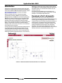
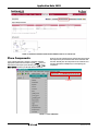
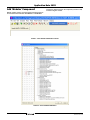
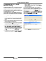
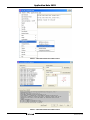
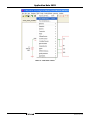
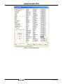
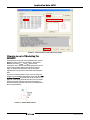
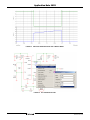
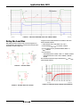
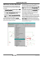
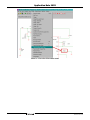
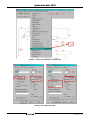
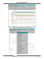
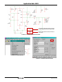
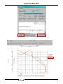
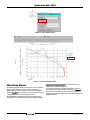
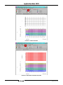
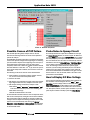
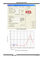
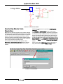
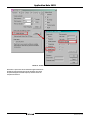
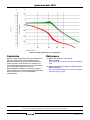
Application Note 1652
Authors: Xuexin Wang and Sameer Dash
iSim:PE User's Guide
Table of Contents
Introduction . . . . . . . . . . . . . . . . . . . . . . . . . . . . . . . . . . . . . . . . . . . . . . . . . . . . . . . . . . . . . . . . . . . . . . . . . . . . . . . . . . . . . . . . . . . . 2
Download a Part's Schematic . . . . . . . . . . . . . . . . . . . . . . . . . . . . . . . . . . . . . . . . . . . . . . . . . . . . . . . . . . . . . . . . . . . . . . . . . . . . . 2
Place Components . . . . . . . . . . . . . . . . . . . . . . . . . . . . . . . . . . . . . . . . . . . . . . . . . . . . . . . . . . . . . . . . . . . . . . . . . . . . . . . . . . . . . . 3
Add 'Websim' Component . . . . . . . . . . . . . . . . . . . . . . . . . . . . . . . . . . . . . . . . . . . . . . . . . . . . . . . . . . . . . . . . . . . . . . . . . . . . . . . . 4
Add MOSFET/Op Amp SPICE Model to Library . . . . . . . . . . . . . . . . . . . . . . . . . . . . . . . . . . . . . . . . . . . . . . . . . . . . . . . . . . . . . . . 5
Change Level of Modeling for MOSFET . . . . . . . . . . . . . . . . . . . . . . . . . . . . . . . . . . . . . . . . . . . . . . . . . . . . . . . . . . . . . . . . . . . . . . 9
Setup the Load Box . . . . . . . . . . . . . . . . . . . . . . . . . . . . . . . . . . . . . . . . . . . . . . . . . . . . . . . . . . . . . . . . . . . . . . . . . . . . . . . . . . . . 11
Add Probes and View Waveforms . . . . . . . . . . . . . . . . . . . . . . . . . . . . . . . . . . . . . . . . . . . . . . . . . . . . . . . . . . . . . . . . . . . . . . . . . 12
Setting Initial Conditions . . . . . . . . . . . . . . . . . . . . . . . . . . . . . . . . . . . . . . . . . . . . . . . . . . . . . . . . . . . . . . . . . . . . . . . . . . . . . . . . 16
Run Simulation . . . . . . . . . . . . . . . . . . . . . . . . . . . . . . . . . . . . . . . . . . . . . . . . . . . . . . . . . . . . . . . . . . . . . . . . . . . . . . . . . . . . . . . . 16
Waveform Viewer. . . . . . . . . . . . . . . . . . . . . . . . . . . . . . . . . . . . . . . . . . . . . . . . . . . . . . . . . . . . . . . . . . . . . . . . . . . . . . . . . . . . . . . 19
Possible Causes of POP Failure . . . . . . . . . . . . . . . . . . . . . . . . . . . . . . . . . . . . . . . . . . . . . . . . . . . . . . . . . . . . . . . . . . . . . . . . . . . 21
Probe Noise in Opamp Circuit . . . . . . . . . . . . . . . . . . . . . . . . . . . . . . . . . . . . . . . . . . . . . . . . . . . . . . . . . . . . . . . . . . . . . . . . . . . . 21
How to Display DC Bias Voltage . . . . . . . . . . . . . . . . . . . . . . . . . . . . . . . . . . . . . . . . . . . . . . . . . . . . . . . . . . . . . . . . . . . . . . . . . . 21
How to Run Monte Carlo Simulation . . . . . . . . . . . . . . . . . . . . . . . . . . . . . . . . . . . . . . . . . . . . . . . . . . . . . . . . . . . . . . . . . . . . . . . 23
Conclusion . . . . . . . . . . . . . . . . . . . . . . . . . . . . . . . . . . . . . . . . . . . . . . . . . . . . . . . . . . . . . . . . . . . . . . . . . . . . . . . . . . . . . . . . . . . . 25
References . . . . . . . . . . . . . . . . . . . . . . . . . . . . . . . . . . . . . . . . . . . . . . . . . . . . . . . . . . . . . . . . . . . . . . . . . . . . . . . . . . . . . . . . . . . . 25
December 21, 2011
AN1652.1
1
CAUTION: These devices are sensitive to electrostatic discharge; follow proper IC Handling Procedures.
1-888-INTERSIL or 1-888-468-3774 | Copyright Intersil Americas Inc. 2011. All Rights Reserved
Intersil (and design) and iSim are trademarks owned by Intersil Corporation or one of its subsidiaries.
All other trademarks mentioned are the property of their respective owners.
Application Note 1652
Introduction
Intersil offers a powerful offline schematic capture and circuit
simulation tool called iSim:PE (short for iSim Personal Edition). It
is based on the SIMetrix/SIMPLIS® simulation platform. The link
to download iSim:PE is located in the iSim™ homepage:
http://www.intersil.com/isim
iSim:PE essentially runs two user-selectable and highly
complementary simulators: SIMPLIS® (for Intersil's Power
Management parts) and SIMetrix® (for Intersil's Op Amp parts).
SIMPLIS® is a leading simulation engine for simulating highly
non-linear systems such as switching power supplies. It uses
piecewise linear analysis techniques to model non-linearity,
which results in transient simulations 10 to 50 times faster than
SPICE [1]. The AC analysis is based on the full time-domain
switching model of the converter, and there is no need to derive
the averaged model of the device.
In order to view the time-domain and frequency domain response
of a switching circuit, the simulation must quickly reach the
steady-state periodic operating point (POP), which is a highly
computationally intensive process. The use of piecewise linear
models helps achieve the desired accuracy in a very short time.
SIMetrix® is a mixed-mode circuit simulation engine. iSim:PE
offers SIMetrix® as a powerful SPICE simulator for Intersil's Op
Amp SPICE models. It is a full-featured schematic entry and
waveform viewer tool.
This application note highlights the most frequently used
functions on iSim:PE that an engineer would need to "virtually
prototype" a circuit design using Intersil parts.
Download a Part's Schematic
When using iSim online tool, once the tool generates the
schematic, you can download it from the design page and design
summary page. The design page is where you can edit the
component values on the schematic and perform simulation as
shown in Figure 1. The design summary page is where iSim
summarizes input requirements, schematic, simulation result
and bill of materials as shown in Figure 2. The "Download
Schematic" tab is located on the top right corner of the two
pages. Once you click the "Download Schematic" tab, you will be
asked to save the file to your PC with extension “.sxsch”.
FIGURE 1. DOWNLOAD SCHEMATIC FROM DESIGN PAGE OF iSim ONLINE TOOL
2
AN1652.1
December 21, 2011
Application Note 1652
FIGURE 2. DOWNLOAD SCHEMATIC FROM DESIGN SUMMARY PAGE OF iSim ONLINE TOOL
Place Components
If it is a simple device like a resistor or capacitor, select the
appropriate symbol from the toolbar or go to Place menu. For
other devices that require a part number, go to Place -> From
Model Library and select your desired device as shown in
Figure 3. Once the symbol has been selected, drag the image of
the component to your desired location on the schematic and
left-click. This will place the component on the schematic. Use
the right-click button or ESCape key to cancel placing the
component.
Tool bar
FIGURE 3. PLACE COMPONENT
3
AN1652.1
December 21, 2011
Application Note 1652
Add 'Websim' Component
iSim:PE contains a library of custom-made components that can
be used with Intersil IC models. Click WebSim -> Add WebSim
components, and then click on the component you want to add,
as shown in Figures 4 and 5.
FIGURE 4. OPEN WEBSIM COMPONENTS LIBRARY
FIGURE 5. SELECT WEBSIM COMPONENT
4
AN1652.1
December 21, 2011
Application Note 1652
Add MOSFET/Op Amp SPICE
Model to Library
The iSim:PE model library contains a comprehensive collection
of MOSFETs for use in both analog/mixed signal as well as power
management applications. It contains over 2000 models for
NMOS parts from various vendors. In addition, the WebSim
library contains generic models for MOSFETs with different levels
of complexity that the user can edit.
It is easy to add a model of another MOSFET to the library. This
feature is useful when the designer has decided on the MOSFET
part number and wants to see more accurate simulation results.
The following steps will guide the user to add the FET model to
the library:
Library -> NMOS as shown in Figure 10. Select the part
number in the library shown in Figure 11 and click Place to
place in the schematic.
The procedure for adding the OPAMP model to the iSim:PE
library is very similar to adding the MOSFET model. There is only
a slight difference when associating the model to the symbol.
Figure 12 shows that you need to select Op-amps from the
Choose Category dropdown box and Operational Amplifier - 5
terminal from the Define Symbol. The number of terminals is the
number of external pins that are defined in your opamp model.
Make sure to Apply Changes before clicking OK.
1. Download the PSPICE model of the MOSFET to your computer.
This can usually be found on the vendor's product website.
The file is typically a '.lib' or '.txt' file containing the PSpice
model.
2. Open the folder containing the PSPICE file; left-click and drag
the file into the iSim:PE Command Shell
FIGURE 6. INSTALL MODELS
3. A message box will pop-up asking if you want to install the file
as shown in Figure 6. Click OK. You will see a confirmation on
the iSim: PE Command Shell as shown in Figure 7.
4. Now, a symbol needs to be associated with this model. Go to
File -> Model Library -> Associate Models and Symbols, as
shown in Figure 8. Choose the category (for example, NMOS)
and symbol (such as, NMOS 3-terminal) corresponding to the
model as shown in Figure 9. Click Apply Changes and then
click OK.
.
FIGURE 7. MESSAGE SHOWING MODEL INSTALLATION IS
COMPLETED
5. The model has now been added to the NMOS library. To place
this MOSFET in the schematic, go to Place -> From Model
5
AN1652.1
December 21, 2011
Application Note 1652
FIGURE 8. ASSOCIATE MODELS AND SYMBOLS STEP 1
FIGURE 9. ASSOCIATE MODELS AND SYMBOLS STEP 2
6
AN1652.1
December 21, 2011
Application Note 1652
FIGURE 10. OPEN MODEL LIBRARY
7
AN1652.1
December 21, 2011
Application Note 1652
FIGURE 11. SELECT A MOSFET MODEL
8
AN1652.1
December 21, 2011
Application Note 1652
FIGURE 12. ASSOCIATE MODELS AND SYMBOLS FOR OPAMP
Change Level of Modeling for
MOSFET
As mentioned in the previous section, SIMPLIS® uses a generic
MOSFET as shown in Figure 13 in simulation. These generic
MOSFETs only model rDS(ON) and CGS (gate-to-source
capacitance), which result in ideal switching waveforms for VDS
(drain to source voltage) and ID (drain current) as shown in
Figure 14. Despite these limitations, they provide a good
approximation of circuit behavior and enable faster simulation
times.
To get more accurate simulation results, you must change the
model level of the MOSFET. Right-click the model and select Edit
Additional Parameters. A small box will pop up, as shown in
Figure 15. If you change the model level from 1 to 2, the model
will include parasitic capacitance of CGS and CDS. Figure 16
shows the switching waveform where there are switching losses
when using model level 2.
FIGURE 13. GENERIC MOSFET MODEL
9
AN1652.1
December 21, 2011
Application Note 1652
FIGURE 14. SWITCHING WAVEFORM USING LEVEL 1 MOSFET MODEL
FIGURE 15. EDIT THE MODELING LEVEL
10
AN1652.1
December 21, 2011
Application Note 1652
FIGURE 16. SWITCHING WAVEFORM USING LEVEL 2 MOSFET MODEL
Setup the Load Box
POP analysis needs a resistive load, as shown in Figure 17, to
converge quickly. The load box is a resistor with a current source
in parallel, as shown in Figure 18.
In Figure 17: Start and Final Current are relative to VOUT and
Source Resistance (RSRC)
• In this example, VOUT = 3.3V, RSRC = R1 = 33Ω
• Current through RSRC: ISRC = 3.3V/33Ω = 100mA
• For the current source in parallel with RSRC, ISTART = 0,
IFINAL = 250mA
• For the load box:
- Actual Start Current = ISTART + ISRC = 0 + 100mA =100mA
- Actual Final Current = IFINAL + ISRC = 250mA + 100mA =
350mA
The simulated waveform in Figure 19 shows the VOUT and ILOAD
plots using this load box.
FIGURE 17. LOAD BOX SYMBOL
FIGURE 18. INTERNAL MODEL OF LOAD BOX
11
FIGURE 19. SIMULATION RESULT SHOWING LOAD TRANSIENT
AN1652.1
December 21, 2011
Application Note 1652
Add Probes and View Waveforms
1. Fixed voltage probe - plots single-ended voltage. Go to Probe
-> Place Fixed Voltage Probe as shown in Figure 20, and put
it at the node you want to look at.
The following example shows how to use this feature to plot four
different probes (VOUT, ILOAD, ILOUT and ICOUT,shown in
Figure 21) in one graph. The last three probes will be plotted in
the same grid as they are all current probes. First, open the Edit
Probe window. Check the box next to Use separate graph and
name the graph. Use the same name, for example, "OUTPUT" for
all these probes. Then, assign ILOAD, ILOUT and ICOUT to the same
grid. To do that, check the box next to Use separate grid and use
the same name; for example, "ILOAD" for these three probes.
2. Fixed inline current probes - plots the current flowing through
it. Go to Probe -> Place Fixed Inline Current Probe and put it
in the wire, as shown in Figure 21.
Figure 24 shows the simulation result. In this graph, all the
current waveforms are plotted on a separate axis, named
"ILOAD", while VOUT is on the default axis.
3. Fixed differential voltage probe - plots the voltage between
two points. Go to Probe -> Place Fixed Differential Voltage
Probe and connect the two points to the positive and negative
input of the probe, as shown in Figure 22.
The second approach is to randomly probe the circuit. This type
of probe is added after the simulation is complete, so it is often
used as a complement of the fixed probes. The most commonly
used types of random probes are the same as fixed probes. Here
we just take a random voltage probe as an example. Go to
Probe -> Voltage (shown in Figure 25), and click the node you
want to look at. This will create a new curve. The random probes
will not be updated after a run, so you must add them manually
every time simulation is complete.
There are two approaches to create plots of simulated results
from a schematic. The first one is to place fixed probes, which
are added before a run. The most commonly used fixed probes
are as follows:
You can edit the properties of the probes in the Edit Probe
window, as shown in Figure 23. The window will appear by
double- clicking the probe. In this window, you can edit the name
and select the axis and graph for each probe.
FIGURE 20. PLACE FIXED VOLTAGE PROBE
12
AN1652.1
December 21, 2011
Application Note 1652
FIGURE 21. PLACE FIXED INLINE CURRENT PROBE
13
AN1652.1
December 21, 2011
Application Note 1652
FIGURE 22. PLACE FIXED DIFFERENTIAL VOLTAGE PROBE
FIGURE 23. EDIT PROBE PROPERTIES
14
AN1652.1
December 21, 2011
Application Note 1652
FIGURE 24. SIMULATION RESULT SHOWING THE PROBES SETTINGS
FIGURE 25. PLACE RANDOM VOLTAGE PROBE
15
AN1652.1
December 21, 2011
Application Note 1652
Setting Initial Conditions
It is advisable to set the initial conditions of switching
components on the schematic; most commonly, capacitor
voltages and inductor currents. Although not necessary, setting
these values helps the simulator to quickly converge to the
periodic operating point.
To set the initial condition, double-click on the component, set
the value (current for inductors and voltage for capacitors), and
check the box for Use Initial Condition.
need to build an average model, which is required in SPICE.
Similar to a network analyzer, iSim:PE uses an AC source and a
Bode probe. As shown in Figure 27, the unit-less AC source
injects a varying frequency signal into the feedback loop. The
Bode probe plots the phase and gain of the circuit.
To run a simulation, go to Simulator -> Choose Analysis, as
shown in Figure 28. The simulation options will show on the right
side of the pop-up window.
A successful POP analysis is required in order to run an AC
analysis. Thus, the POP check box is automatically checked when
AC is checked. Under the AC tab, you can change the sweep
frequencies and points per decade.
Figure 29 shows the analysis parameters for a Transient
simulation. Normally, you only need to change the "stop time"
and keep the other default settings. Note that you need to check
the box next to POP manually when only running Transient
analysis. Click OK to save all the settings.
FIGURE 26. SETTING INITIAL CONDITIONS
Run Simulation
iSim:PE uses the SIMPLIS/SIMetrix® simulator, which is a circuit
simulator designed for rapid modeling of switching power
systems, while SIMetrix® is a mixed-signal simulator based on
SPICE. Here we focus on the introduction of a running simulation
in SIMPLIS®. There are three simulation options in the iSim:PE
SIMPLIS® simulator: POP, AC and Transient. POP stands for
Periodic Operating Point. It finds the steady-state limit cycle, or
the periodic operating point of a periodically switching system,
without having to simulate the entire power-up sequence. This
dramatically speeds up the analysis of the design's behavior
under different load conditions [1].
iSim:PE has the ability to perform small signal analysis and
provide the Bode plot of the control loop for the switching power
supply circuit. If you run a POP analysis before AC, there is no
16
Click Run from the drop-down menu of Simulator or press F9 to
run simulation. The status window shown in Figure 30 appears.
You can click Abort to terminate the simulation. If you check the
box next to Close on completion this window will close
automatically after the simulation is done.
Simulation graphs will be plotted in the waveform viewer. Graph
cursors can be used to make measurements from waveforms.
Go to Cursors -> Toggle On/Off to switch the cursor display on or
off. A hint box will show up for first-time users.
In the example shown in Figure 31, we move the second cursor to
the point where the closed loop gain equals 0dB. The
corresponding frequency is the bandwidth of the system, and the
phase value is the phase margin. Note that, in this plot, what is
shown as phase is actually phase margin. If you want to plot
phase in the simulation result, you must change the Bode probe
setting before running simulation.
Double clicking the Bode probe opens the Edit Device
Parameters window shown in Figure 32. Check the box next to
"Multiply by -1". Figure 33 shows the AC simulation result where
phase is plotted instead of phase margin.
AN1652.1
December 21, 2011
Application Note 1652
The unit-less AC source injects a varying
frequency signal into the feedback loop
Bode probe plots the Phase and Gain of
the circuit
FIGURE 27. AC SOURCE AND BODE PLOT PROBE
FIGURE 28. CHOOSE ANALYSIS
FIGURE 29. TRANSIENT ANALYSIS SETTINGS
17
AN1652.1
December 21, 2011
Application Note 1652
FIGURE 30. SIMULATION STATUS
Phase Margin is 67.8°
FIGURE 31. USE CURSORS TO READ PHASE MARGIN AND BANDWIDTH
18
AN1652.1
December 21, 2011
Application Note 1652
FIGURE 32. BODE PROBE SETTINGS
Phase is -112°
@Gain= 0dB
FIGURE 33. BODE PLOT SHOWING PHASE
Waveform Viewer
The following example shows how to move a curve to a separate
grid and how to apply measurement to the curves in the
waveformviewer. In this example, we want to look at VPHASE.
Click the New Grid tab in the tool bar, as shown in Figure 34, and
a new grid will be created in the waveform viewer.
Select VPHASE by checking the box next to the legend which
designates the curve. Select the new grid by clicking it. Click the
19
Move Curve to Selected Axis/Grid tab in the tool bar. Now
VPHASE is in the new grid (Figure 35).
If you want to perform an accurate measurement, select the
waveform by checking the checkbox and then go to Measure in
the menu bar. In this example we measured the frequency of
VPHASE (Figure 36). The measurement result is shown under the
legend of the curve.
AN1652.1
December 21, 2011
Application Note 1652
FIGURE 34. CREATE A NEW GRID
FIGURE 35. MOVE CURVE TO SELECTED AXIS/GRID
20
AN1652.1
December 21, 2011
Application Note 1652
FIGURE 36. MEASURE FREQUENCY
Possible Causes of POP Failure
Probe Noise in Opamp Circuit
POP (Periodic Operating Point) analysis works on the full
time-domain switching model of the circuit and is required to
perform AC analysis.
This example shows how to plot noise in SIMetrix®. First open
the Choose Analysis window, as shown in Figure 37. Make sure
you select Noise simulation in the Analysis Mode. You can define
the sweep frequency and output node. Then run the simulation.
The SIMPLIS® simulation engine takes a snapshot of all inductor
currents and capacitor voltages at the beginning of one switching
cycle and another snapshot at the beginning of the next cycle (a
clock-edge trigger or POP-trigger is used to capture these
snapshots). It then tries to find a set of initial conditions that will
drive this difference to less than ~10-10% [2]. The closer you are
to the actual steady-state conditions, the sooner the circuit will
reach POP.
The following are the most common causes of POP failure:
1. Initial conditions (of capacitor voltages, inductor currents,
etc.) are too far from their steady-state values.
2. Circuit is not stable.
3. POP trigger is not connected to a proper node so that a trigger
signal is generated once every complete conversion cycle
4. POP analysis settings constrain the analysis so that:
a.Max Period (Menu -> Simulator -> Choose Analysis ->POP)
is less than the conversion period of one switching cycle.
b.Max Period is too large.
The noise waveform does not come out automatically after the
simulation is done. Go to Probe AC/Noise -> Plot Output Noise. If
you are sitting at the transient waveform before plotting the
noise, the noise figure will be shown in a separate graph.
However, if you are looking at the Bode plot, the noise will be
plotted on the same graph, with a different Y-axis. Figure 38
shows the simulated noise for ISL28191 at unity gain. It shows
that the noise is 1.7nV/√Hz at 1kHz, which is the same as the
specification in the ISL28191.
How to Display DC Bias Voltage
You can view DC operating point results by placing markers on
the schematic as shown in Figure 39. Go to Place -> Bias
Annotation. To place voltage markers at all nodes select, Auto
Place Voltage Markers. The DC voltage at each node will be
shown at the sharper side of the marker after each simulation
run. This option, however, clutters up the schematic so you may
prefer to place markers manually by selecting Place Marker.
c.Number of POP iterations is too small.
For most iSim:PE schematics with the correct component values,
POP can be reached just by setting the correct initial conditions.
Run only Transient analysis (without any change in LOAD) long
enough so that the important switching waveforms in the circuit
appear to have reached steady state. Then go to Options->
Simulator -> Initial-Conditions -> Back-annotate. This will assign
steady-state initial conditions to all components and make the
circuit reach POP faster.
21
AN1652.1
December 21, 2011
Application Note 1652
FIGURE 37. CHOOSE NOISE ANALYSIS
FIGURE 38. OUTPUT NOISE FIGURE OF ISL28191
22
AN1652.1
December 21, 2011
Application Note 1652
Voltage Marker
FIGURE 39. PLACE VOLTAGE MARKER
How to Run Monte Carlo
Simulation
Similarly set the tolerance for capacitors in Set All Capacitor
Tolerances to 5%.
Monte Carlo is a method of analysis that uses random sampling
techniques to obtain a probabilistic approximation to the solution
of a mathematical equation or model. Using this same approach
applied to the resistors and capacitors will show the effect of
parameter variations. The following example uses Monte Carlo to
look at frequency response and step response when component
values are not exact values but with tolerance.
First, set tolerance for the resistors and capacitors. Go to
Monte-Carlo -> Set All Resistor Tolerances. Enter the tolerance
value in the pop-up window. In Figure 40, we use 2% for the
resistors.
Go to Simulator -> Choose Analysis to open up the analysis
settings window shown in Figure 41. To view the set parameters
for the types of analysis simulated, click on each tab located at
the top of the Choose Analysis window. On the right side of the
window, you are able to view, which analysis types are enabled.
To enable the Monte Carlo analysis in the AC simulation, click the
Enable Multi Step box in the Monte Carlo and multi-step analysis
section. Click Define to open up the Define Multi Step Analysis
window.
Set the sweep mode to Monte Carlo and enter the Number of
steps, which shows in Figure 41 Number of steps set to 30.
.
FIGURE 40. SET TOLERANCES
23
AN1652.1
December 21, 2011
Application Note 1652
FIGURE 41. ENABLE MONTE CARLO ANALYSIS
Click "Run" or press F9 to run the simulation. Figure 42 shows an
example of gain and phase plots for AC simulation. They show
the passband ripple and cutoff frequency variation due to the
components tolerance.
24
AN1652.1
December 21, 2011
Application Note 1652
FIGURE 42. MONTE CARLO RESULTS OF AC SIMULATION
Conclusion
References
iSim:PE is a powerful offline simulator which complements the
iSim online design simulation tool. This application note
illustrates the most frequently used functions in iSim:PE as a
quick user’s guide. It is not intended to be a complete user’s
manual of iSim:PE. For any function that is not mentioned here
or for more detailed instructions please see the
Simetrix/SIMPLIS User Manual [1]. If you have any questions
about using iSim:PE, please contact Intersil Central Applications:
email:[email protected] or tel: 1-888-INTERSIL
(1-888-468-3774).
[1] SIMetrix Technologies Ltd., User's Manual SIMetrix/SIMPLIS,
http://www.simetrix.co.uk/Files/manuals/6.0/UsersManu
al.pdf
[2] SIMetrix Technologies Ltd., "What is the difference between
SIMPLIS and Spice?"
http://www.simplistechnologies.com/resources/suppleme
ntary/diff_simplis_spice.pdf
Intersil Corporation reserves the right to make changes in circuit design, software and/or specifications at any time without notice. Accordingly, the reader is
cautioned to verify that the Application Note or Technical Brief is current before proceeding.
For information regarding Intersil Corporation and its products, see www.intersil.com
25
AN1652.1
December 21, 2011