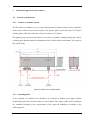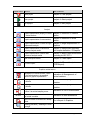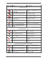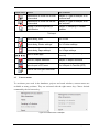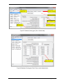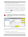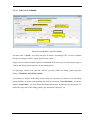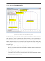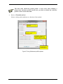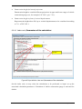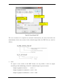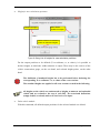
1
Technische Universität Dresden Chair of Rail Vehicle Technology Institut für Bahntechnik GmbH Branch Office Dresden V ersion 2.3 for Windows XP, V ista and 7 Program system for calculation of rolling stock construction gauge User manual Copyright © 1999-2011 by Technische Universität Dresden Institute of Rail Vehicle Engineering Chair of Rail Vehicle Technology 01062 Dresden Germany Phone: 0351 / 463 366 74 Fax: 0351 / 463 365 90 E-Mail: [email protected] Institut für Bahntechnik GmbH Branch Office Dresden Wiener Straße 114-116 01219 Dresden Germany Phone: 0351 / 877 59 0 Fax: 0351 / 877 59 90 E-Mail: [email protected] All rights reserved. No part of this handbook may be reproduced or processed, copied or distributed by means of electronic media in any form without explicit approval by the Chair of Rail Vehicle Technology at the TU Dresden and the Institut für Bahntechnik (IFB). The regulations of the software license contract are valid for the application of the manual at the same time. All product names used are regarded as registered trademarks of the corresponding firms. Issued 01 August 2011 (3nd translated revision) / program version 2.3 E-Mail: Internet: DIMA user manual [email protected] www.software-dima.de Page 2 of 150 Table of contents 1 Installation......................................................................................................................... 6 1.1 Requirements for installation ........................................................................................ 6 1.2 Installation procedure .................................................................................................... 6 1.2.1 How to install the DIMA software ......................................................................... 6 1.2.2 How to install and use the software dongle ............................................................ 9 1.3 Upgrade / Update of an available DIMA version ....................................................... 11 1.3.1 Upgrade of version 1.x ......................................................................................... 11 1.3.2 Update of version 2.x ........................................................................................... 12 2 Program concept ............................................................................................................. 13 3 Calculation approach of the software ........................................................................... 17 3.1 General considerations ................................................................................................ 17 3.1.1 Vehicle co-ordinate system .................................................................................. 17 3.1.2 Rounding rules ...................................................................................................... 17 4 5 3.2 Calculations carried out on a single vehicle ................................................................ 19 3.3 Definitions to calculate articulated train sets .............................................................. 20 3.4 Calculation of vehicles with active tilting system ....................................................... 22 3.5 Calculation of static bogie displacement ..................................................................... 25 3.6 Calculation of vehicle end geometry and coupler deflection ...................................... 25 How to run the program ................................................................................................ 26 4.1 Menu bar ..................................................................................................................... 26 4.2 Toolbars ....................................................................................................................... 28 4.3 Context menus ............................................................................................................. 31 4.4 Actions in graphic windows ........................................................................................ 32 Program description ....................................................................................................... 33 5.1 Set up program and program help ............................................................................... 33 5.1.1 Program options.................................................................................................... 33 5.1.2 Printer settings ...................................................................................................... 35 5.1.3 Online help and information dialog for the DIMA program ................................ 35 5.2 Databases ..................................................................................................................... 36 5.2.1 How to handle databases - fundamentals ............................................................. 36 5.2.2 Database „Vehicle body“...................................................................................... 39 5.2.2.1 General data .................................................................................................. 40 5.2.2.2 Data for articulated train set modules ........................................................... 43 5.2.2.3 Data for end wall calculation ........................................................................ 43 5.2.2.4 Data for pantograph calculation according to UIC and EBO ....................... 44 DIMA user manual Page 3 of 150 5.2.3 Database „Running gear“ ..................................................................................... 45 5.2.3.1 General data - running gear .......................................................................... 47 5.2.3.2 Lateral bogie/body plays and lateral plays ................................................... 51 5.2.3.3 Vertical displacements in the lower range .................................................... 51 5.2.3.4 Inclination of vehicle around longitudinal axis ............................................ 53 5.2.3.5 Dimensions of the running gear.................................................................... 54 5.2.4 Database „Tilting system“ .................................................................................... 55 5.2.5 Database „Reference profile“ ............................................................................... 58 5.2.6 Database „Roll centre height and vehicle flexibility coefficient“ ........................ 60 5.2.6.1 Database edit window for entry of measured values .................................... 62 5.2.6.2 Dialog „Determine roll centre height and …“ ......................................... 63 5.3 Project definition ......................................................................................................... 67 5.3.1 General.................................................................................................................. 67 5.3.2 Data required for possible partial analyses ........................................................... 68 5.3.3 Project definition structure ................................................................................... 70 5.3.3.1 Index card „Project information“ ............................................................... 70 5.3.3.2 Index card „Vehicle“.................................................................................... 71 5.3.3.3 Index card „Datasets vehicle/module“ ..................................................... 72 5.3.3.4 Index card „Reference profile“................................................................... 75 5.3.3.5 Index card „Parameters of the calculation“ ............................................. 79 5.3.4 Test, start and exit the analysis of a project .......................................................... 90 5.4 Graphic analysis window ............................................................................................ 91 5.4.1 General.................................................................................................................. 91 5.4.2 Print and export graphics ...................................................................................... 92 5.4.3 Analysis graphics „Vertical section (X-Y plane)“ ............................................... 94 5.4.3.1 Management of vertical sections and display features ................................. 94 5.4.3.2 Sampling of a vertical section ...................................................................... 98 5.4.4 Analysis graphics „Cross section (Y-Z plane)„ .................................................. 100 5.4.4.1 Configure display features .......................................................................... 100 5.4.4.2 Sampling of a cross section ........................................................................ 103 5.4.5 Analysis graphics „Bogie displacement“ ........................................................... 105 5.4.6 Analysis graphics „Vehicle end geometry and coupler deflection” ................... 107 5.4.7 Analysis graphics „Buffer head dimensions“ ..................................................... 110 5.5 Total report ................................................................................................................ 111 5.5.1 General handling................................................................................................. 112 5.5.2 Configuration of report in the dialog „Report elements“ ................................ 112 5.5.2.1 Index card „Elements“............................................................................... 112 5.5.2.2 Index card „Calculation positions for reduction“ ................................... 113 5.5.2.3 Index card „Calculation positions pantographs“ ................................... 119 5.5.2.4 Index card „Output positions bogie“ ....................................................... 120 5.5.2.5 Index card „Output positions end wall“ .................................................. 121 5.5.3 Output values and tables of the total report ........................................................ 122 5.5.3.1 Cover and input variables ........................................................................... 122 5.5.3.2 Result output for bogie displacement ......................................................... 122 5.5.3.3 Result output for buffer head dimensions................................................... 122 DIMA user manual Page 4 of 150 5.5.3.4 Result output for vehicle end geometry and coupler deflection ................. 123 5.5.3.5 Result output reduction............................................................................... 123 5.5.3.6 Result output for pantographs according to UIC ........................................ 126 5.5.3.7 Result output for pantographs according to EBO ....................................... 127 5.5.4 Print and export total report ................................................................................ 128 5.6 3D-Export .................................................................................................................. 128 5.6.1 Index card parameters ......................................................................................... 129 5.6.2 Wireframe ........................................................................................................... 131 5.6.4 STEP-target file .................................................................................................. 133 6 Examples ....................................................................................................................... 134 7 Program validation ....................................................................................................... 135 8 Glossary and indices ..................................................................................................... 136 8.1 Keywords .................................................................................................................. 136 8.2 Figures ....................................................................................................................... 139 8.3 Tables ........................................................................................................................ 141 Annex A Symbols of input- and output variables.......................................................... 142 Annex B Allocation of input variables and program calculation modes..................... 146 Annex C Basics for calculation ........................................................................................ 148 Annex D Error handling .................................................................................................. 150 Icons You must pay attention to all warnings, hints, as well as limitations of inputand output options. You may pay attention to hints in terms of program handling, as well as calculation methodologies. DIMA user manual Page 5 of 150 1 1.1 Installation Requirements for installation To run the DIMA program, the following system requirements have to be fulfilled: – Processor: min. Pentium 300 MHz (Athlon or Duron, Intel Celeron and others are also compatible), – RAM: min. 64 MB, – Free hard disk memory: min. 30 MB, – Operating system: Windows XP or higher – Screen resolution: min. 1024 x 768 (min. 800 x 600), – USB port (for dongle). 1.2 Installation procedure The program installation under Windows only works with the rights for access to the necessary system resources. To obtain them, please contact your system administrator. 1.2.1 How to install the DIMA software Start „SETUP.EXE“ from CD-ROM and follow the instructions by the installation assistant. DIMA user manual Page 6 of 150 Figure 1: Setup assistent for DIMA installation Figure 2: Input of user information DIMA user manual Page 7 of 150 Figure 3: Choice of target folder Figure 4: Choice of start menu folder DIMA user manual Page 8 of 150 Figure 5: Invocation of DIMA installation Figure 6: Completion of DIMA installation 1.2.2 How to install and use the software dongle The HASP SRM driver software for the software protection plug (dongle) starts automatically during the DIMA installation. Don’t plug-in dongle before installing the driver. DIMA user manual Page 9 of 150 Figure 7: Setup assistant to install dongle driver After an information dialog, the following dialog windows are called to install the driver software: Figure 8: Start of driver installation DIMA user manual Page 10 of 150 Figure 9: Completion of driver installation Figure 10: Invocation to connect dongle Before starting the DIMA program, plug-in dongle on USB interface of the PC. Working with the DIMA program is impossible without dongle. After finishing the DIMA installation, you may start the program upon the selected program link. 1.3 Upgrade / Update of an available DIMA version 1.3.1 Upgrade of version 1.x Starting with the introduction of DIMA 2.0, the developers changed the database format (among others necessary to be run under MS Windows VistaTM). The IFB GmbH Dresden / DIMA user manual Page 11 of 150 TU Dresden converted the database of the preceding DIMA version 1.x. It is stored on the upgrade CD. Carry out upgrade on your computer as follows: Uninstall the old „DIMA.EXE“ incl. dongle plug, Install the new „DIMA.EXE“ incl. dongle plug, Copy converted DIMA-2.x-database file: – Create a backup of the installed, empty database file „Dima.mdb“. Depending on the operating system, you find them in the database directories below: – Windows XP: C:\Document and Settings\All Users\IFB\Database Windows Vista / 7: C:\Users\Public\Documents\IFB\Database Copy the converted database file „Dima.mdb“ from directory „Database“ of the upgrade CD into the database directory specified above. 1.3.2 Update of version 2.x If you have already installed a version of DIMA 2.x, you have to perform the update achieved on your computer: Execute the file „UPDATE.EXE“ on installation medium. You are guided through the installation procedure by an assistant. The Update will only be carried out, if there is a former DIMA version available on your system. For updates, please pay attention to the corresponding hints on the installation medium handed over. DIMA user manual Page 12 of 150 2 Program concept The DIMA program is designed to calculate the main vehicle dimensions according to the current German and European regulations. Since these regulations may be generalised, you will be able to use this program also for vehicles to be exported worldwide. However, it is necessary to check in each case, whether special regulations exclude such an application or not. DIMA allows performing the following operations: Calculation of vehicle construction gauge for standard-gauge railway vehicles, that defining the length-, width- and height dimensions of the vehicle bodies and running gears according to the kinematic and static methods. The calculations underlie the following regulations: – UIC 503 (7th issue of February 2007), – UIC 505-1 (10th issue of May 2006), – UIC 505-5 (2nd issue of January 1977), – UIC 506 (1st issue of January 2008), – EBO (Railway Building and Operational regulations, issued in 1992), – TE (issued in 1938) and – The Russian standard GOST 9238-83 (issued in 1983). However, the static calculation according to TE (in contrast to the kinematic method according to UIC), which is no longer common practice in Europe, may still be important for special applications and export. Calculation of vehicle construction gauge for standard-gauge- articulated trains. The calculation methodology considers the regulations below: – UIC 505-1 (10th issue of May 2006), – UIC 505-5 (2nd issue of January 1977), – UIC 506 (1st issue of January 2008), – EBO (issued in 1992) and – TE (issued in 1938). DIMA user manual Page 13 of 150 Calculation of vehicle construction gauge for pantographs according to the regulations UIC 505-1 and EBO §9 and Annex 3. Calculation of bogie displacements under the vehicle in horizontal and vertical directions, without taking into consideration pitching and rolling on the springs. The analyses are based on the determination of the pitch and yaw angles according to the former GDR standard, named TGL 32439/01. To investigate the buffer head geometries according to UIC 527-1 (3rd issue dated April 2005). To analyse the end wall geometry and coupler deflections in curve radius and s-curve. Here it is possible to investigate the rail configuration of an s curve with intermediate straight upon determination of a virtual curve radius. Calculation is performed according to Friedrich from the wagon manufacturing company Waggonbau Bautzen. The program’s basic intent is to work with projects, on the one hand. On the other hand, it foresees database-oriented recording of input data. A project describes the composition of all input data and definitions, which are needed to carry out the calculation types selected. Projects can be stored and called again/ changed at each time. Database-oriented work enables free and convenient access to the data already entered. This way, one may investigate variants for suitable vehicle main dimensions to the desired extent. Handling of files has highest priority. Exact results and optimised dimensions can only be guaranteed upon complete and exact input data. Internal plausibility data checks by means of validators support the user and avoid long PC sessions due to false inputs. The option to check projects on completeness excludes false results due to missing initial data. In DIMA, output of results is given upon monitor, connected local or network printers, as DXF file for further processing in CAD programs, and as RTF text file to be taken over into text processing- and documentation programs. Furthermore, it is possible to export the calculation results for further processing in table calculation programs. Numerous graphs and diagrams make it possible to evaluate the investigation results in a convenient manner and to export the graphs with the results upon established interfaces. The program is engineered under Windows XP and Vista and offers structure and handling as they are known from the Windows family (WIN 2000, XP and Vista). DIMA user manual Page 14 of 150 Due to a comprehensive online help, also first users can achieve good progress in the use of this handbook. In addition to this help, we offer the program user interface and the issue of the total report in English language. The next program versions may be implemented in other languages by request. The DIMA program is also fitted with a multi language user interface and report output. DIMA user manual Page 15 of 150 In principle, the program is run according to the following sequence: 1. Program start 2. Generation of a project Generate a new project Open an available project1) 3. Definition of the project parameters General information Type of vehicle, Data of tilting system Vehicle body, running gears of the vehicle modules Reference profile (calculation method) Additional parameters for reduction calculation Parameters for the further calculations Databases Tilting system1) Vehicle body Running gear Reference profile Roll centre height and vehicle flexibility coefficient1) 4. Test and start of the project 5. Project analysis – Presentation of results Calculation of vehicle construction gauge (vertical section, cross section, report tables) Calculation of bogie displacement (graphics, tables) Calculation of vehicle end geometry and coupler deflection (graphics, tables) Calculation of buffer head dimensions (graphics, tables) Total report for all analyses Possible evaluations: Onscreen graphical evaluation (data samping) DXF-export of vehicle cross sections1) Printout of the results Report export as RTF-file1) 6. End of program 1) not available in the Demo version Figure 11: Operation sequence DIMA user manual Page 16 of 150 3 3.1 Calculation approach of the software General considerations 3.1.1 Vehicle co-ordinate system For the vehicle co-ordinates, we use a three-dimensional co-ordinate system, whose origin lies in the point of intersection of wheel plane (X-Y plane), plane of the rail centre (X-Z plane) and the plane of the end wall or the vehicle’s head part (Y-Z plane) . The guiding cross section is that vehicle cross section, on which a leading running gear, that is a running gear that determines the adjustment of the vehicle in the track channel, is pivoted on the vehicle body. Figure 12: Definition of co-ordinate system 3.1.2 Rounding rules In the program, all variables for calculation are declared as floating point digits (double mathematical precision). Interim values are not rounded. The output results of the calculation are rounded according to the requirements of the approval authorities according to the following rules: DIMA user manual Page 17 of 150 Table A: Rounding rules Results of bogie displacement calculation: Yaw and pitch angles wh, wv1, wv2: rounded down to 2 decimal positions Results of the calculation of vehicle construction gauge: b, br, bz-b, h, hr, k/hs, na;ni, Point: Mathematically rounded to millimetre (3 decimal positions) bz: rounded down to millimetre (3 decimal positions) Ea;Ei: Final result rounded up to millimetre (3 decimal positions) z: rounded up to tenth of a millimetre (4 decimal positions) Example: Rounding the calculated width bz = 1.5749999999998 m down to 3 decimal positions brings the output value 1.574 m. Calculation results for the reduction of pantographs … … according to UIC: na; ni, Point: Mathematically rounded to millimetre (3 decimal positions) j’, z’, z’’: Mathematically rounded to tenth of a millimetre (4 decimal positions) Ei’;Ea’, Ei’’;Ea’’: rounded up to millimetre (3 decimal positions) h25kV, b25kV/2: rounded down to millimetre (3 decimal positions) … according to EBO: R, v: Mathematically rounded to meter or kilometre/hour Ue, Uef: Mathematically rounded to millimetre (3 decimal positions) All values of the table: Mathematically rounded to tenth of a millimetre (1 decimal position) DIMA user manual Page 18 of 150 Calculation results for buffer head geometry Minimum width of buffer head: Mathematically rounded to millimetre Calculation results of vehicle end geometry and coupler deflection dB: Mathematically rounded to millimetre (3 decimal positions) Gamma, Gamma1, Gamma2: Rounded up to 2 decimal positions H, H1, H2: Mathematically rounded to millimetre (3 decimal positions) Omega, Omega1, Omega2: rounded up to 2 decimal positions u, u1, u2: rounded up to millimetre (3 decimal positions) w, w1, w2: rounded down to millimetre (3 decimal positions) z, z1, z2: rounded down to millimetre (3 decimal positions) 3.2 Calculations carried out on a single vehicle With the DIMA program, you may carry out the following operations for a single vehicle: to calculate vehicle construction gauge, to analyse vehicle end geometry and coupler deflection, to calculate bogie displacement, as well as to determine buffer head geometry. The options for calculations are based on the regulations referred to in Chapter 2. It is possible to calculate single vehicles, as well as articulated train sets described in the following chapter, also with active tilting system. Moreover, the DIMA software is able to consider not only various running gears on a vehicle, but also running gear eccentricities. DIMA user manual Page 19 of 150 3.3 Definitions to calculate articulated train sets With the DIMA program, one may calculate articulated train sets with a wide variety of module combinations inside the articulated train set. We distinguish the following types of basic modules: Figure 13: Definition of basic module types Possible design types for articulated train sets are shown in the figure below: Figure 14: Articulated trains – example DIMA user manual Page 20 of 150 As a rule, we have only few knowledge of the concrete adjustment of the articulated train set’s modules in the rails, since, in most cases, we don’t know the influence of the stabilizers over the joints and, unless all axles are driven, also uneven longitudinal force paths have an influence across the train length. For this reason, calculation of vehicle construction gauge is based on each worst case position. Starting at the first module whose radial adjustment of vehicle in curved tracks is determined (that is the first module with two running gears), we calculate the vehicle construction gauge in a common way und thus find out the worst case precalculated deflections caused by the radial adjustment of the forerunner module for the follow-up modules. For each – In comparison with a traditional vehicle – missing running gear, we have to find out two precalculated deflections caused by the radial adjustment of the forerunner module (max. positive and max. negative). When having determined all missing precalculated deflections caused by the radial adjustment of the forerunner module at one module, it is possible to calculate vehicle construction gauge – by changing the equations for geometric overthrow – like for a standard-single vehicle. Calculation is carried out correspondingly for all other connection modules. This approach results in the first boundary condition in the calculation of articulated train sets: Articulated train sets may only be calculated, if the whole articulated train set is determined in terms of its curve geometry. This condition is fulfilled, if the number of running gears under all hinge modules is at least by 1 (one) greater than the number of the hinge modules. The used destination of precalculated deflections caused by the radial adjustment of the forerunner module excludes an articulated train set configuration with two sequenced modules determined in their curve geometry (two modules of type 2 – also two short-coupled single vehicles). At this position, it is necessary to consider the articulated train set in a separate manner. This is the second boundary condition when modelling articulated train sets: It is impossible to represent articulated train sets with two sequenced modules of type 2. At this position, the articulated train set has to be considered in a separate manner. DIMA user manual Page 21 of 150 3.4 Calculation of vehicles with active tilting system The calculation of vehicles with active tilting system as it is implemented in the DIMA program is mostly based on Annex F of the UIC 505-1. However, it was necessary to integrate extensions, since the calculation according to the Annex above may only be applied to cross sections near the vehicle middle and near the end wall. Incorrect exceeding of the reference profile may occur, in particular in cross sections near the guiding cross sections, calculated according to Annex F. For the range of GOST standards, it is impossible to calculate vehicles with tilting system. Tilting system calculation in the DIMA program assumes four reduction ranges: – Ea,u reduction outside, bottom; introduction in calculation theory, since the values to the outside of the curve are deciding in the lower overhang range, – Ea,o reduction outside, top; introduction in calculation theory, since the values to the inside of the curve are deciding in the upper overhang range, – Ei,u reduction inside, bottom; introduction in calculation theory, since the values to the outside of the curve are deciding in the lower range between the guiding cross sections, – Ei,o reduction inside, top; introduction in calculation theory, since the values to the inside of the curve are deciding in the upper range of the guiding cross sections. This distinction became necessary caused by the different approach to calculate the lateral play in the overhang and in the range between the guiding cross sections. Furthermore, it is necessary to pay attention to the different values of quasi-static inclination to the outside and inside of the curve. To consider tilting systems with changing tilting centre, we may enter several tilting systems (see Chapter 5.2.4). Calculate vehicle construction gauge for tilting system for each tilting state X as follows: – Find out a vehicle construction gauge for the reduction to the inside of the curve with corresponding z value and the play approach according to the position of the cross section DIMA user manual Page 22 of 150 just investigated, without taking into account the rotation due to tilting system. That means, in calculation, there are only considered the other position in the curve and the rolling motion to the outside of the curve due to quicker passage of a curve. Line X1a is created. – Rotation of line X1a around the roll centre with tilting angle. Line X2a is created. – Cutting and mirroring of the line X2a at the center line. The resulting gauge X3a for the determination of reduction to the inside of the curve develops. – Find out a vehicle construction gauge for reduction to the outside of the curve with corresponding z value and the play approach according to the position of the cross section just investigated, without taking into account the rotation by the tilting system. That means, only the other position in the curve and the stronger rolling motion by quicker passage of a curve are included. Gauge X1b is created. – Rotation of line X1b around the roll centre with tilting angle. Line X2b is created. – Cutting and mirroring of the line X2b at the center line. The resulting gauge X3a for the determination of reduction to the outside of the curve develops. – Superposition of the resulting gauges for all considered tilting states (lines X3a, X3b, Y3a, Y3b, …) with the line from standard calculation of vehicle construction gauge and, if necessary, with the hitherto resulting vehicle construction gauge from another tilting system. The resulting vehicle construction gauge for vehicles with tilting system is formed. DIMA user manual Page 23 of 150 Figure 15: Determination of vehicle construction gauge for vehicles with tilting system The strategy described above elucidates that the determination of reduction on vehicles with tilting system is a numerically performed graphic determination of lines. Since this determination demands a lot of computational efforts, it may result in slightly increased computation times at PCs of less computing capacity. In the DIMA program, we may consider the maybe other play approach of the lateral play to the outside of the curve at quicker passage of a curve with tilting system. Annex F to UIC 505-1, on which the tilting system calculation is based, assumes that inclined vehicles take an outer chord position or centre position in the curve. Since it is sometimes impossible to give unambiguous predictions for the curve position, in particular for vehicles in banking mode (banked), we introduced the alternative between a calculation according to Annex F of the UIC and according to the approach by the TU Dresden: – „Annex F“: assumes the lateral bogie/ body plays for curve passage in outer chord position for the vehicle or all modules of an articulated train set, – “Approach by TU Dresden“: assumes the worst case when the lateral plays come together. DIMA user manual Page 24 of 150 3.5 Calculation of static bogie displacement Exploration of bogie displacements relies on the GDR standard according to TGL 32 439/01. Starting from the calculation of the pitch and yaw angles, we find out the limit positions of each bogie in vehicle-X-Y- (horizontal) and -X-Z directions (vertical). The horizontal limit position represents the bogie’s area demand with the rectangular dimensions - length and width of the running gear (see Chapter 5.2.3.5) - at horizontal turning off. The vertical limit position stands for the available installation area taking into account turning off around the pitch angle, starting from a rectangular area to be kept free with the sizes length by height of the running gear. In general, the vertical turning off results in different angles for the range pivot point plane vehicle centre and the range pivot point plane next end wall. This is due to the different position of the bogie when entering ramp against ramp exit. Calculation and representation does not consider the vehicle’s rolling- and pitching motions on its springs. 3.6 Calculation of vehicle end geometry and coupler deflection With the DIMA program, you may calculate the vehicle end geometry of standard-gauge railway vehicles. To do this, the vehicle is coupled with itself, and, when passing a simple curve, it is analysed as a simple curve- and curve- s curve combination. You may also compute the vertical end wall offset by concave transition passage. The calculation is based on finding out the geometric vehicle adjustments appearing thereby by a mathematical approach. In this calculation, the values of the coupler deflections are obtained indirectly. DIMA user manual Page 25 of 150 4 How to run the program Having started the DIMA program, the user gets to the user interface. It consists of the menu bar and the tool bars at the upper screen margin, as well as the working area situated below. 4.1 Menu bar The menu bar is changed as a function of the opened and activated edit windows. „File“ menu Using the commands in the „File“ menu, it is possible to create, open, close and save projects, as well as save them as a file of another name. Furthermore, the „File“ menu includes commands to export graphics in the bitmap (*.BMP) or vector formats (*.WMF), as well as reports in the rich-text format (*.RTF). In the „File“ menu, you may also find commands to set up the pages of a report, for printer settings, and last, but not least, to print reports. „Database“ menu Upon the „Database“ menu, you may access to the program’s databases. The choice is limited to the following items: Vehicle body, Running gear, Tilting system, Reference profile, as well as Roll centre height and vehicle flexibility coefficient. „Analysis“ menu In the „Analysis“ menu, all commands for test, start and exit of project analysis are arranged. You also find commands to access to the single analysis windows: Reduction (vehicle construction gauge), Bogie displacement, DIMA user manual Page 26 of 150 Vehicle end geometry and coupler deflection, Buffer head dimensions and Total report. „Windows“ menu The „Windows“ menu includes commands to layout the currently opened windows, which may also be switched over in this menu. „Options“ menu In the „Options“ menu, you may enable/ disable the current toolbars or invocate the dialogs „Program“ and „Database connection“. The user may also choose the program language. Figure 16: Choice of the database connection Choice of program language Figure 17: Choice of program language „Help“ menu You may invocate online help and an information dialog about the program upon the „Help“ menu. DIMA user manual Page 27 of 150 4.2 Toolbars For default, during program start, the toolbars Database, Project and Analyses are shown. After starting the analysis of a project, in the „Analysis“ toolbar, there are additionally indicated the icons X-Y graphics, Y-Z graphics, as well as Total report. Table B: Toolbar buttons Toolbar button Function Menu command Database Database „Vehicle body“ Database Vehicle body Database „Running gear“ Database Running gear Database „Tilting system“ Database Tilting system Database „Reference profiles“ Database Reference profile Database „Roll centre height / vehicle flexibility coefficient“ Database Roll centre height and vehicle flexibility coefficient Project Create a new project File New project Open an existing project File Open project Save an opened project File Save project as Close an opened project File Close project DIMA user manual Page 28 of 150 Toolbar button Function Menu command Test a project Analysis Test project Start a project Analysis Start project Exit a project Analysis Exit project Analysis Graphic representation (display) of results Analysis reduction vertical of vertical sections section Graphic representation of cross sections Analysis reduction cross section Graphic representation of results of bogie Analysis bogie displacement displacement analysis Graphics Graphic representation of vehicle end geometry analysis results Analysis Vehicle end geometry and coupler deflection Graphics Graphic representation of buffer head dimensions analysis results Analysis Buffer head dimensions according to UIC 527-1 Open total report window Analysis Total report 3D-STEP-Export Analysis 3D model output (STEP-Export) Graphics vertical section Management of vertical sections, choice of the vertical section to be sampled, features of graphic representation Evaluation Management of vertical sections Sampling of the chosen vertical section in Evaluation Sampling in X X direction direction Sampling of the chosen vertical section in Evaluation Sampling in Y Y direction direction Representation of the cross section on position X at vertical sampling cursor No icon Evaluation Go to cross section Representation of the main dimensions of Evaluation Main dimensions the vehicle / modules Export of chosen cross sections in bitmap File Export Graphics format Enabling (Activation) / Disabling the zoom rectangle DIMA user manual Page 29 of 150 Toolbar button Function Menu command Graphics cross section Management of cross sections, choice of Evaluation Management of cross the cross section to be sampled, features sections of graphic display Export of chosen cross sections in DXF format File Export DXF Export of chosen cross sections in bitmap File Export Graphics format Evaluation table of cross sections (reduction results) Evaluation Tables Sampling of chosen cross section in Z direction Evaluation Sampling in Z direction Representation of vertical section on position Z on vertical sampling cursor Evaluation to vertical section Activation / Deactivation of the zoom rectangle - Graphics bogie displacement Choice of the running gear to be represented Analysis Type of analysis (Choose running gear) Display of bogie displacement in horizontal direction (X-Y plane) Analysis Type of analysis horizontal turning off Display of bogie displacement in vertical direction (X-Z plane) Analysis Type of analysis vertical turning off Sampling of bogie displacement in X direction Analysis Sampling in horizontal direction Sampling of bogie displacement in Y direction Analysis Sampling in vertical direction Graphics vehicle end geometry and coupler deflection Representation of end wall distances in curve Analysis Type of analysis in curve Representation of end wall distances in s curve Analysis Type of analysis in s curve Representation of end wall distances in inclination changes Analysis Type of analysis in inclination change DIMA user manual Page 30 of 150 Toolbar button Function Menu command Representation on vehicle front end wall / Analysis Type of analysis on chosen module front end wall Representation on vehicle rear end wall / chosen module Analysis Type of analysis on rear end wall Sampling of vehicle end geometry in vertical direction Analysis Sampling in vertical direction Total report Invocate dialog „Print“ File Print Invocate dialog „Printer settings“ File Printer settings Invocate dialog „Page settings“ File Page settings Switch to another page 4.3 Arrow key, <Figure up>- and <Figure down> key Select box „Report elements“ Analysis Report elements Export of report in RTF format File Export Text file (RTF) Choice of one of the given zoom levels - Context menus To accelerate your work in the databases, projects and result windows, context menus are available at many positions. They are activated with the right mouse key. Choose desired command by the left mouse key. Figure 18: Context menus - examples DIMA user manual Page 31 of 150 4.4 Actions in graphic windows In the available graphic windows, such as the graphic windows of the cross- and vertical section sampling, you may zoom up and down sections, shift zoomed parts and partially graphically sample the curve paths. To use these functions, we need special keyboard- and mouse key combinations, which are listed below: Scaling up/ -down (zooming) in graphic windows Scale up region: Keep pressed <Switch>- (<Shift>-) key and select the region to be scaled up by keeping pressed the left mouse key. Cancel zoom: Keep pressed <Switch>- (<Shift>-) key and click with left mouse key in graphic window. Shift zoomed sections: Move mouse pointer to the margin of the graph. Zoom section is shifted into this direction according to the chosen page or corner. Move sampling bar Move by mouse: The sampling bar moves under the mouse cursor at pressed <Alt> key on the keyboard. Move via keyboard: At pressed <Alt> key, the arrow keys or <Figure up>and <Figure down> keys move the sampling cursor. The <Figure up>- and <Figure down> keys move the cursor in 10-cm increments, and the arrow keys in 1-mm increments. You may also call the Zoom function via toolbar. DIMA user manual Page 32 of 150 5 5.1 Program description Set up program and program help 5.1.1 Program options Go to the „Options“ dialog upon the menu commands „Options“ „Program“. Information of author and company in projekt definition Standard path for openning and saving of projects Figure 19: Program options, index card „Project“ All changes carried out in the program options are saved during exit of the dialog by „OK“ and are considered at once or at each new start of the program. The entries in the fields „Editor“ and „Firm“ are taken over for default at new projects into the analogue fields of the index card „Project“ of the project definition. It is possible to define a standard-like directory to open and save projects upon the entry field „Standard project directory“ or the corresponding button. DIMA user manual Page 33 of 150 Number of calculation positions for vertical sections Figure 20: Program options, index card „Calculation“ The „Number of calculation positions per module“ defines the quantity of cross sections in vehicle-X direction, which are calculated for the representation of a vertical section. The number selected here is in relationship with the option „Recalculation while sampling“ of index card „Model features“ of the „Management“ dialog in the analysis graphics „Vertical section“ (see Chapter 5.4.3.1). The maximal number of calculation positions is limited to 1,000. Figure 21: Calculation or interpolation of points on vertical sections When interpolating points of the reference profile, the result may differ from the real value as a function of the number of calculation positions. The number of calculation positions immediately acts on the calculation speed when creating vertical sections. Calculation times may become merely high in case of vertical sections of articulated train vehicles with tilting system, if we have many calculation positions (>500) and computers of low or medium efficiency, only. DIMA user manual Page 34 of 150 5.1.2 Printer settings You may get to the „Printer settings“ dialog upon menu „File“ or the corresponding button on the toolbar of the report window. Choose or set up printer upon a Windows standard dialog with corresponding select buttons to choose one of the connected devices and to set up the printer chosen. 5.1.3 Online help and information dialog for the DIMA program Get to the online help for the DIMA program upon the menu commands „Help“ „Content“. A standard help dialog with the index cards „Content“, „Index“ and „Search“ is indicated. In principle, you may call the online help in all dialogs, entry-, analysis- and graphic windows also with the <F1> key. For the majority of entry elements in the windows, direct invocation of the specific help item is supported (context-sensitive help). Get to the information dialog for the DIMA program upon the menu commands „Help“ „Information about Dima”. Information of program version Licensed modules Information of operating system Figure 22: Dialog „Information about DIMA“ DIMA user manual Page 35 of 150 In the information dialog related to the DIMA program, you may request for all information about the program version, not only about the licensed modules, but also information about the operational system. Program version and licensed modules are information that is particularly needed during trouble tracking by the support department. 5.2 Databases 5.2.1 How to handle databases - fundamentals The DIMA program concept is based on working with databases, which do, on the one hand, enable convenient data storage and updating, and are a basis for a flexible composition or synthesis of projects. The databases to be edited independently of the project are another base for calculation of variants, which is made possible by the software technological implementation of simultaneous sessions carried out at a number of projects. The single vehicle or the modules of an articulated train set are separated into the essential elements vehicle body, running gear and tilting system and the corresponding data are managed in separate databases. The data volumes managed separately are brought together in the project definition (see Chapter 5.3). The characteristics roll centre height and vehicle flexibility coefficient arising from the combination of vehicle body and running gear are saved in the database „Running gear“. Each dataset should have an unambiguous dataset identifier, upon which you may identify this dataset in the corresponding edit window and in the project definition. Maximum character length of the dataset identifier is 255 characters. Each dataset identifier may only be used one time in the corresponding database. During saving, it is checked whether the dataset identifier has been assigned multiply; if yes, this is pointed out to the user. The databases are edited in all database edit windows according to the same procedure. With a database navigator, you may move in the database, as well as create and delete datasets. DIMA user manual Page 36 of 150 New dataset Delete Rename Save Dismiss dataset datatset inputs inputs Dataset name Search dataset Figure 23: Database navigator New dataset: Inserts a new dataset before the current dataset. Delete dataset: Deletes the current dataset. Rename dataset: Changes the name of the current dataset. Save entries: Saves the changes carried out on the current dataset up to now. Only active, if dataset in edit mode. Reject entries: Cancels editing of the current dataset (undo) and recovers the state before the changes. Only active if dataset in edit mode. Search for dataset: When entering the dataset identifier, in case of consistent root word, search for the desired dataset is simplified. When inserting a new dataset, you may copy existing original datasets and save them under a new name. Taking over the values into the new dataset, which is associated with this DIMA user manual Page 37 of 150 procedure, simplifies work and supports calculation of variants, in which only a few parameters have to be changed. Copying is carried out by creating a new dataset (button) and activation of the select box „Copy ‘…‘”. In the databases „Vehicle body“ and „Running gear“, you may immediately call a dataset section upon the command „Go to dataset“. According to the choice, the entry list in the right dialog box is moved to the desired section. The dialog „Create filter“ is also indicated in the menu bar of the databases „Running gear“ and „Reference profile“. This dialog enables filtering of the listed datasets according to a characteristic feature. Database „Running gear“: You may filter the list of datasets to be selected with the entries „Single-axle running gear or similar construction type“ or „Multi-axle running gear“ in the menu, so that only the corresponding running gear types are indicated. Database „Reference profile“: With the entries in the menu, you may filter the list of reference profiles to be selected, so that only the lines of a certain calculation method are indicated. You may choose among the reference profiles according to UIC, TE, GOST and UIC 503. The database edit windows include the entry fields for all values of the corresponding database summarised in one individual dataset. In the database edit windows, there is no vehicle type- or calculation-depending reduction in the data volume to be entered. Thus, for instance, you may determine the running gear as driven or not driven in the database „Running gear“, although this information had only to be entered for the calculation of the vehicle construction gauge of powered vehicles. In single cases, hints about the concretely necessary input values are given in the handbook or the program help. Before starting an analysis, the program checks the project data on completeness and points out missing data. DIMA user manual Page 38 of 150 The description of the database edit windows in the following chapters offers one possible strategy for data entry for a project. In general, sequence of entries is any desired. In all databases, validators avoid to enter invalid data that is data situated outside the range of commonly permissible data. 5.2.2 Database „Vehicle body“ The database edit window „Vehicle body“ is subdivide into the sections General data, Data for articulated train set modules, Data for end wall calculation and Data for pantograph calculation and may be accessed to upon the menu command „Database“ „Vehicle body“ or the corresponding button on the toolbar. Dataset name (identifier) Remarks to dataset Input of the required datas in the given unit Calculation of Gsv an Slv for longitudinally symmetric vehicles Figure 24: Database „Vehicle body“ (Part 1: General data) DIMA user manual Page 39 of 150 Dates for articulated train sets Input of the required dates in the given unit Selection of nominal power supply for pantograph calculation Figure 25: Database „Vehicle body“ (Part 2: Special data) The input fields in the sections are inside a window moveable upon the vertical scrollbar, in which you may choose the sections or input fields to be edited. Navigate to the individual sections also with menu button „Go to dataset“. 5.2.2.1 General data Length over buffer LP The value ‚length over buffer’ is required to find out the chain dimensioning the vehicle geometry of single vehicles / hinge modules (articulated modules) (see Figure 26), as well as to determine buffer head geometry. Length body LWk Enter length of the upper parts above sheet metal or, for some wagon types, length above head part, whereas the entered value must not be greater than the length over buffer. In articulated train set modules, hereunder, we understand the distance between vehicle endwalls of the corresponding articulated train set module. Bogie pivot/ wheelbase distance a Bogie pivot/ wheelbase distance is the distance between the end wheelsets of the vehicles without bogies or between the pivots of vehicles with bogies. DIMA user manual Page 40 of 150 For vehicles that don’t have a fixed pivot, a virtual pivot is graphically determined as point of intersection of the longitudinal centre lines of bogie and vehicle body, if the vehicle is located concentrically in the 150-m curve with evenly spaced plays. The distance of the virtual pivot from geometric centre point is named as eccentricity (see Chapter 5.2.3.1) of the running gear. At vehicles without bogies, in which the wheelsets are eccentrically articulated, a is also regarded as the distance between the wheelsets. Define position of the actual rotation points upon entry of eccentricity of the running gear. In articulated train set modules with one or without any running gear, bogie pivot/ wheelbase distance may also be zero. Distance buffer/hinge point – front end wall GSv Definition of the distance between buffer section or coupler centre or hinge point at articulated vehicles and the end wall at the defined front end wall of vehicle or the hinge module. In standard wagons, this value corresponds to the buffer length. Vehicle overhang from running gear, front end SLv Definition of the distance from end wall and articulation of the running gear or the pivot on the defined front of the vehicle / hinge module. In longitudinally symmetric single vehicles and hinge modules of type 2, you may automatically determine Gsv and Slv upon the button „Longitudinally symmetric“. Static asymmetry eta Static asymmetry eta specifies the angle, which would be formed by the vertical centre line of the vehicle body and the perpendicular, if the vehicle stands on the horizontal rail, without any friction. It may result from a lack of construction, a false adjustment of suspension and unevenly distributed loads. Consequently, one should assume a value of 1° for vehicles to be built. For vehicles whose normal load is adjusted more unbalanced than in the compartment coach (side gangway carriage), one has to determine static asymmetry by tests, and to consider the maximal value of the empty and loaded vehicle. If a measurement was performed, then the measured value for the calculation of the vehicle construction gauge is deciding. DIMA user manual Page 41 of 150 The values of the distance buffer/hinge point – end wall and the distance end wall – running gear define asymmetric single vehicles / hinge modules of type 2, as well as hinge modules of type 1, and are defined as follows: Figure 26: Definition of chains dimensioning vehicle- / module geometries For hinge modules of type 0, the values SLv and a are not significant. DIMA user manual Page 42 of 150 Cross traverse of loading unit qLE For traffic with continental wagons running in Great Britain, the turning bolt of the British Railways (BR) allows 6 mm cross traverse of loading unit. If 100 M 2196 0015 bolts are used for the wagon UIC-jigger pin according to ERRI B 112/RP 7 and RP 8 and UIC/ERRI drawing, a cross traverse of 12.5 mm is to be used. For this reason, when using UIC-jigger pins, a reduction of 6.5 mm is required on both sides (UIC 503, Annex B.2.1). 5.2.2.2 Data for articulated train set modules Hinge point height front hv /hinge point height rear hh Enter hinge point heights on front and rear at each module. These values are considered in the lower calculation of vehicle construction gauge of the articulated train sets, on the one hand. On the other hand, these values are taken to check correct sequencing of the modules. Enter values only for articulated train set modules. These values do not describe buffer height at single vehicles. This height is requested in Chapter „Data for end wall calculation“. 5.2.2.3 Data for end wall calculation Roof-edge height above buffer hD / buffer height hP Enter height of roof edge (highest position of the arched roof) above buffer middle or buffer height above Rp. Roof-edge radius RD Radius of the roof edge (fillet) to the end wall. Entry is only necessary for end wall calculation or to analyse buffer head dimensions (buffer height). If there are not entered values in Chapter „Data for end wall calculation“, then the program analyses the end wall in buffer height and maximal reference profile height. DIMA user manual Page 43 of 150 5.2.2.4 Data for pantograph calculation according to UIC and EBO Pantograph flexibility index t The pantograph flexibility index describes lateral displacement of the pantograph bow lifted to 6.50 m when applying a force of 300 N. (Calculation of vehicle construction gauge is based on a value of 0.03 m.) Pantograph construction- and installation tolerance tau The tolerance for constructing and installing the pantograph is the permitted deviation from the vehicle body’s centre line and the middle of the pantograph bow lifted to 6.50 m. (Calculation of vehicle construction gauge is based on a value of 0.01 m.) Adjustment tolerance vehicle suspension Theta The adjustment tolerance of vehicle suspension is that inclination, the vehicle body may take due to installation defects of suspension, if the vehicle stands still unloaded on a horizontal rail. (Entry in radian! Calculation of vehicle construction gauge is based on a value of 0.005) Pantograph lower articulation installation height ht Installation height of the lower pantograph articulation above Rp. Half width of pantograph bow bw Width of pantograph bow according to UIC 608. According to UIC 608, the following widths ( 2 bw ) are permitted: – 1.,45 m: SSB, FS, SNCF (25 kV), CFL (25 kV), – 1.60 m: BR, SNCF (25 kV), SNCF (1,5 kV), – 1.95 m: CFL (3 kV-), CSD, DB, DSB, MAV, NS, ÖBB, PKP, SNCB, SNCF (1,5 kV-), VR, (DR) Pantograph calculation according to UIC: You must enter the half width of pantograph bow only for evaluation in the Y-Z graph (cross section). This value does not affect the pantograph verification according to UIC. Choice of nominal power supply for calculation according to UIC When operating the powered vehicle under nominal power supply of 25 kV, a safety distance of 170 mm from the reference profile is to be kept for uninsulated live parts. DIMA user manual Page 44 of 150 When selecting button „25 kV AC“, the table with the results includes the maximally permitted width for these parts beginning from a height of 3 m above RS. Choice of nominal power supply for calculation according to EBO Defining the nominal power supply of the pantograph, you may consider the defined dimensions of the lineside structure gauge for the corresponding electricity system in the EBO, Annex 3, and the minimum distances from the overhead contact wire when calculating the reference contour width of the pantograph. These entries are only required for pantograph calculation. 5.2.3 Database „Running gear“ Get to the database edit windows upon menu command „Database“ „Running gear“ as well as the corresponding button on the toolbar. The database edit window „Running gear“ is subdivided into the sections General data, Lateral bogie/ body plays and lateral plays, Vertical displacements, Vehicle inclination around the longitudinal axis and Running gear dimensions. DIMA user manual Page 45 of 150 Input window for dataset search Dataset name (identifier of dataset) Remarks to dataset Selection of running gear configutation Selection for powered bogie Input of the required dates in the given unit Figure 27: Database „Running gear“ (Part 1: General data) Input of the required datas in the given unit Figure 28: Database „Running gear“ (Part 2: Plays, vertical displacements) DIMA user manual Page 46 of 150 Calculate or determine in database for existing vehicles the values for roll centre and flexibility coefficient Input of the required datas in the given unit Figure 29: Database „Running gear“ (Part 3: Tilting, dimensions) The input fields in the sections are situated in a window to be moved via vertical scrollbar, in which you may click the sections to be edited or the input fields. Navigation to the single sections may also be done upon menu button „Go to“. 5.2.3.1 General data - running gear Running gear type Choose among single-axle and multi-axle running gear. Single-axle running gears are understood as free steering wheelsets, as well as single-axle special designs (single wheel-single running gears, single-axle running gears with a special running gear frame and, if necessary, multi-stage suspension). When changing the choice of the running gear type, then the two follow-up input fields are also changing – both in the database and in the project definition. For single-axle running gears, Eccentricity and Tangential deviation of a single-axle running gear, for multi-axle running gears, Bogie wheelbase and Eccentricity are requested. Bogie wheelbase p Distance between end wheelsets in the bogie. In case of more than two wheelsets in the bogie, put in distance between the outermost wheelsets. DIMA user manual Page 47 of 150 Eccentricity e Eccentricity is defined as a longitudinal deviation of the running gear pivot point from the common centre position in the running gear. The value is signed. Sign is defined as follows: Figure 30: Definition of signed eccentricity (type of module 2) DIMA user manual Page 48 of 150 Figure 31: Definition of signed eccentricity (type of module 1) As a rule, running gear of module type 1 is regarded as a leading running gear. Tangential deviation of a single-axle running gear phi (only single-axle running gears) Describes the angle of a possible torsion of a single wheelset against the exact radial adjustment in the curve (standard values: 3 ... 5°). DIMA user manual Page 49 of 150 Figure 32: Tangential deviation phi of a single-axle running gear Half distance between secondary suspension springs b2 Half distance between secondary suspension springs b2 is required for kinematic calculation of the vehicle construction gauge according to UIC 505-1, to find out the values in the lower region (supporting polygon, UIC 505-1 (7.1.1, Fig. 10)). Maximal track gauge lmax. lmax0, nominal track gauge l, Outer distance between wheel flanges d Enter maximal track gauge with track extension in curve (in the region of standard-track railways being members of the UIC, this size is 1.465 m for mainlines and 1.470 m for minor lines), maximal track gauge in the straight rail (this value is only needed for the calculation of vehicle construction gauges according to GOST), nominal track gauge (1.435 m for standard-track railways of the UIC), as well as outer distance between wheel flanges of the wheelsets 10 mm below the rolling wheel (normal case 1.410 m). Regarded as driven ( > 0,2) During the calculation of driven vehicles, running gear is regarded as driven or not driven, depending on friction coefficient during starting . Different positions of the driven vehicle in the groove of the rails during curving result here from. According to UIC 505, Par. 7.2.2.1: – 0,2: they are regarded as driven, – < 0,2: regarded as not driven. DIMA user manual Page 50 of 150 5.2.3.2 Lateral bogie/body plays and lateral plays Axle bow lateral play q Axle bow lateral play stands for the transverse displacement between wheelset and bogie frame or between wheelset and vehicle body according to each side (for vehicles with single wheelsets). Measure axle bow lateral play immediately at wheelset bearing, where all components are maximally worn. In free steering wheelsets, axle bow lateral play includes also the deflection of the wheelset holders. Lateral bogie/ body play in straight rail w0 The lateral bogie/ body play describes possible transverse displacement of bogie pivot and bolster out of the centre position to each side in the straight rail. Measure lateral bogie/ body play immediately on the significant components, where they are maximally worn. Description of lateral bogie/ body play (as a function of curve) Lateral bogie/ body plays depending on the curve describe the possible transverse displacement of bogie pivot and bolsters out of the centre position to each side, each as a function of the rail curve radius and the displacement direction. The radiuses demanded by the UIC - 150 and 250 m – are offered as a standard entry for bogie/ body plays. Enter up to 5 additional radiuses and lateral bogie/ body plays. – R [m]: Radius (rail curve radius), at which lateral bogie/ body play changes as a function of the rail curvature. – wi(R) [m]: Possible transverse displacement towards inside curve. – wa(R) [m]: Possible transverse displacement towards outside curve. 5.2.3.3 Vertical displacements in the lower range Total of maximal vertical wear dimensions v Maximal values of all permissible vertical wear limits that occur between 2 corrections (maintenance activities), in particular maximal wear of wheels, transoms or similar. for deflection values dz, dz30, sfs and sfp: When calculating the vertical deflection values, we obtain the additional lowering for the four zones of the supporting polygon (UIC 505-1, Annex 5) only from the effect of the lowering of the deflection difference between the states „Loaded“ and – depending on vehicle type - „Loaded with overload“ or „Loaded to maximum“. That means, for the additional deflections, static DIMA user manual Page 51 of 150 deflection is set equal to „Minimal suspension load“. The UIC wording is thus understood as load in the state „Loaded“. As a result, entire lowering for one of the 4 zones of the supporting polygon is composed of static deflection dz and additional deflection for the corresponding zone. Static deflection (Difference empty – loaded) dz Static deflection (in meters) of the vehicle is the feasible lowering of the vehicle body between the operational states „Empty“ and „Loaded“ on the suspension (springs). The value includes the deflection on primary- and secondary springs. The value is to be entered for a correct calculation of the lower construction gauge (height) for all vehicle types. for deflection values dz30, Sfs and Sfp: According to UIC 505-1, Chapter 7.1.1.2.2.2, for maximal suspension deflection, we should assume deflection at 30 % overload or the full deflection. Coping with a demand of the EBA, the UIC wording „or“ is to be understood in a way that the maximal value of these both suspension deflections has to be introduced in the calculation, each. Suspension deflection at 30 % Overload dz30 Deflection at 30 % overload of the sprung weight. This value represents the whole suspension deflection from the empty vehicle to the loaded vehicle (loaded with 30 % overload). The longitudinal deflections under the impact of the permitted increased load (increased by 30 %), which have to be considered for wagons into the height reduction (vehicle construction gauge), are not considered in the DIMA software. Maximum primary spring deflection Sfp Enter spring deflection (primary) as a difference of the path between the empty vehicle body and the stop of the maximal spring deflection. During calculation of lower height reduction (vehicle construction gauge), the value is used to define the maximal values to be assumed for spring deflection for coach cars and luggage van, as well as wagons and special wagons. Maximum secondary spring deflection Sfs Enter spring deflection (primary) as difference of deflection between empty vehicle body and the stop of maximal spring deflection. During calculation of lower height reduction (vehicle construction gauge), the value is used to define the maximal values to be DIMA user manual Page 52 of 150 assumed for spring deflection at coach cars and luggage vans, as well as (if with secondary spring) for wagons and special wagons. In special vehicles with a bogie with single stage suspension (Sfs1 = 0) and a bogie with two stages of suspension (Sfs2 > 0), the entire vehicle is regarded as with two stages of suspension. Transom play J In bogie wagons, whose transom play is less or equal to 0.005 m, we may assume that asymmetry eta = 1° includes this play. In bogie wagons, whose transom play exceeds 0.005 m, this phenomenon has to be considered for quasi-static displacement, and is particularly to be specified there. For passenger vehicles and powered vehicles / multiple units, J may be neglected and set to 0. In this case, it is unnecessary to enter bG (half distance between the transoms). Half distance between the transoms bG Distance between the transoms (from transom middle to vehicle middle), in order to consider transom plays in quasi-static displacement Vertical resilience ko Vertical resilience or displacement is determined, thereby taking into account dynamic upward displacement for an unloaded (unoccupied), runable vehicle without wear. In this case, upward motion of the vehicle due to vertical displacements is considered. 5.2.3.4 Inclination of vehicle around longitudinal axis Roll centre height of vehicle hcl, hcb Roll centre height C is defined as a point of intersection of the vehicle centre lines in Z direction of the normal co-ordinate system (according to UIC 505-1; Par. 4.1) of the untilted vehicle body and the tilted vehicle body, which is tilted due to a transverse force acting in parallel to wheel plane. Its distance from top of rail (RS) is named as roll centre height hc. Distinguishing the empty (hcl) and loaded (hcb) vehicle considers relative displacement of roll centre height, since the height difference of this roll centre height does not necessarily coincide with deflection dz of the vehicle. Vehicle flexibility coefficient sl, sb If a vehicle stands on a superelevated rail, whose wheel plane is located to the horizontal under an angle , then its vehicle body is inclined on its suspension and forms an angle ß DIMA user manual Page 53 of 150 with the vertical to wheel plane. The ratio s = / is named as vehicle flexibility coefficient. Figure 33: Roll centre height and vehicle flexibility coefficient on vehicle Determination of the value used in the calculation from the both roll centre heights is carried out according to the „Instruction for kinematic calculation of vehicle construction gauges...“ by the BZA Minden. For the calculation of reduction, use the greater vehicle flexibility coefficient (see also Annex C). The values of roll centre height and vehicle flexibility coefficient can be calculated according to a UIC computation technique (UIC 505-5) and approximately found out by means of the vehicles listed in the database. The button DETERMINE calls a corresponding calculation- and selection dialog (Chapter 5.2.6.2). 5.2.3.5 Dimensions of the running gear We need the dimensions of the running gear for calculation of bogie displacement due to passing curves and inclination changes. The entries for the running gear sizes are unnecessary if no calculation of bogie displacement has to be carried out. DIMA user manual Page 54 of 150 Length lFw, width bFw and height hFw of the running gear Enter maximal length, width and height of the running gear (in meters). From these values, a cuboid sphere is defined; turning this cuboid around the corresponding yaw and pitch angles, it provides the limit positions or the available installation area of the bogie. Pivot point height LW at vehicle body hAn, wheel diameter dL, wheel flange height hSk Pivot point height (articulation height) of the running gear at vehicle body and wheel diameter are needed for the calculation of yaw angle (vehicle-X-Y plane) and pitch angle (vehicle-X-Z plane) of bogies according to TGL 32439/01. (Wheel flange height and wheel diameter are a reference size to check the building height of the running gears). 5.2.4 Database „Tilting system“ In the DIMA program, we implemented only the calculation method for active tilting systems. Calculation of the share of the quasi-static displacement z is carried out according to the assumptions for active tilting systems in Annex F of UIC 505-1. Dataset name (identifier of dataset) Remarks to dataset Maximum cant devicienty Input of the required datas in the given unit Figure 34: Database „Tilting system“ Entry of different tilting system states is done upon data table „List of tilting states“. You may add and delete tilting system states upon the <+> and <–> keys in the headline of the data table. Maximum cant deficiency- Way and Works department ic Enter cant deficiency related to the characteristics of the location of line (radius, speed), or enter maximally permitted cant deficiency for vehicles with tilting system. Each DIMA user manual Page 55 of 150 railway system defines its own maximum value for its railway line. Normally, values from 0.09 to 0.18 m are used (UIC 505-1, Annex F). A maximal cant deficiency of 0.15 m is permitted in the range of German railways according to EBO (§ 40). For tilting system vehicles, there exists an unlimited exceptional allowance, which permits a cant deficiency of 0.30 m acting on the vehicle on suitable railway lines. These railway lines must be adapted to traffic with tilting system in any case. For this reason, it is possible to use cant excess values considered by the Way and Works department that are greater than 0.15 m. Tilting angle beta Enter that angle that is adjusted by the tilting system at associated cant excess ip, under which the vehicle rotates around the associated inclination centre. The angle to be entered here is the angle adjusted by the tilting system control, but not the effective tilting angle (adjusted tilting angle minus roll angle). The angle to be entered here is the angle of the tilting system adjusted by the control, but not the effective tilting angle (adjusted tilting angle minus roll angle). Cant excess ip Enter cant excess, at which tilting system of the vehicle adjusts tilting angle . Centre height h0 Enter height of rotation (centre height) above RS, around which the tilting system rotates at cant excess ip under an angle . This centre is regarded as lying stringently on the vehicle’s cross section centre. Roll centre height hc, vehicle flexibility coefficient s Enter roll centre height and vehicle flexibility coefficient, around which or by which the vehicle rolls during curving with cant excess ip. The hc value may be measured or calculated. If the transverse displacements of the vehicle body are greater than the free plays underframe/bogie, then it has to be measured at the height of the bogie stops; if it is impossible neither to measure nor to calculate this parameter, assume a compounded value h c = 0.5 m. (UIC 505-1, Chapter 7.1.3) DIMA user manual Page 56 of 150 Bogy/ body play wa, max. It might be the case that special lateral bogie/ body plays are foreseen for the inclined vehicle body. Enter maximal value of lateral bogie/ body play to the outside of the curve (in meters) for the current tilting system. The specified value is valid for all running gears of the vehicle. Pantograph tilting angle alpha Enter angle in the tilting system for pantographs. As a function of the kind of pantograph tilting, the following determinations are valid for the tilting angle: 1. Enter no tilting angle for pantographs that do not incline with the vehicle body, 2. For pantographs, which incline together with the vehicle body and which are equipped with a counter-tilting system, it is necessary to enter the pantograph tilting angle, 3. For pantographs on vehicles without tilting system, which have an own centering system, it is necessary to enter the tilting angle. Flexibility factor of pantograph supporting frame Sn Due to the immoderate transverse displacement value of the bow on tilting system vehicles, one has to mount the pantographs on supporting frames that do not incline with or are equipped with active shifting elements. For the flexibility factor of the supporting frame of the pantographs, 2 cases have to be discriminated (UIC 505-1, Annex F.7): 1. Pantographs on frameworks (such as ETR 460 FIAT): the value for sn is related to this framework, 2. Pantographs with active shifting elements. The flexibility factor of the supporting frame sn results from the value of vehicle flexibility coefficient s of the vehicle body. Pantograph tilt centre height when tilted hp For a tilting system, enter centre height of the pantograph in meters above RS, around which the pantographs incline through the tilting system under a tilting angle. If there is no entry for vehicle flexibility coefficient, roll centre height or lateral bogie/ body play, then these entries are regarded as zero. DIMA user manual Page 57 of 150 5.2.5 Database „Reference profile“ In contrast to all the other edit windows, the numbers to be entered in database edit window have to be specified in millimetres [mm]. This copes with the view of the UIC. Database navigator Enter password Dataset name (identifier of dataset) Associated calculation method Input of profile points Reference profile graphic Figure 35: Database „Reference profile“ The term „reference profile“ is used as a synonym both for the reference profiles of the kinematic calculation of vehicle construction gauge and the boundary lines of the static calculation of vehicle construction gauge. During program installation, read-only reference profiles are provided. They are protected by a password, and it is impossible to delete them. It is possible to backup each reference profile individually created with a password to avoid undesired changes. Input or edit a password for the current reference profile is performed with the command „Edit password...“ from the menu or the icon. To edit a protected line, enter password at first. Associated calculation method Each reference profile has to be connected with a corresponding calculation instruction. The link is obtained by this select box. You may choose among: DIMA user manual Page 58 of 150 – – Calculation according to UIC (kinematic reduction) with: Reference profile according to UIC 503, Reference profile according to UIC 505-1, Extended gauges GA, GB and GC according to UIC 506. Calculation according to TE issued in 1938 (lower gauge according to TV, static reduction) with: – Reference profile of the TE, Extended gauges GA, GB and GC of TE according to UIC 506. Calculation according to GOST 9238-83 (static reduction, Russian standard) with: Gauge T, Tc, Tpr, 1-T, Gauge 0-VM, 02-VM, Gauge 01-VM, Gauge 03-VM. The sequence described above is simultaneously the sorting order when sorting reference profiles in terms of the calculation method. Normal co-ordinates Y and Z Describe the horizontal distance of the reference profile’s vertex from its longitudinal centre line or the vertical distance from the reference profile’s vertex to the horizontal axis referring to the wheel plane (RS). Vertical oscillation ratio hs For parts of the vehicle laying above 3,250 mm, there is determined an oscillation ratio hs, considering dynamic displacement, which, in turn, considers – Vertical oscillations (upward), – Perpendicular components of quasi-static displacement, as well as – Transverse displacements. Enter sign according to direction of the normal co-ordinates Z (such as hs = -30 mm). Following curve radius R Considers the existence of curved representations of the reference profiles, as they appear, for example, in the Technical Unity of Railroading (TE), and in reference profiles of foreign railway administrations. The curve path is represented by the points n, n+1 and the corresponding radius. Point n describes the start co-ordinates (Y(n), Z(n)) of the curve. Point n+1 with the end co-ordinates (Y(n+1), Z(n+1)) limits the curve and DIMA user manual Page 59 of 150 represents – by specifying the curve radius – the curve, whereby positive radiuses describe a reference profile segment arched to the outside. 5.2.6 Database „Roll centre height and vehicle flexibility coefficient“ In the stage of development and design, it is impossible to measure roll centre height h c and vehicle flexibility coefficient s of a vehicle. For theoretical determination, the UIC 505-5 includes a calculation method, which demands very detailed knowledge of the vehicle’s design data, in particular of the running gear. The so-called VKZ method was created within the scope of a Diploma project performed at the Institute of Rail Vehicle Engineering at the TU Dresden. The abbreviation VKZ stands for comparison index and connects the three significant influencing parameters with s and hc. These are the weight of loaded vehicle body G2, gravity height of the loaded vehicle body h2 and spring stiffness of the secondary suspension stage c2. VKZ G2 h2 c2 We assume that the weight of the vehicle body G2, which acts on the lever h2, brings out a moment of the force on the suspension springs. It is necessary that a suitable spring stiffness counteracts this moment. In vehicles with geometrically identical running gears (commensurable properties of the vehicles), upon these three parameters, one may also compare the values of vehicle flexibility coefficient s and roll centre height hc. With a comparison index (VKZ) of a known and surveyed vehicle and the comparison index (VKZ) of the vehicle to be investigated, it is possible to find out a value for the vehicle flexibility coefficient s in a relatively simple and exact manner by the following rule of three: sx sx, VKZx: sd, VKZd: sd VKZ x VKZd Values of the new vehicle Value of the vehicle out of the database The s and hc values of the database are only related to the loaded vehicles, since the vehicle flexibility coefficient sd as a value to be assumed for the VKZ method never drops down during loading, and the z value is directly proportional to the vehicle flexibility coefficient. It DIMA user manual Page 60 of 150 is also possible to determine roll centre height hc with VKZ, however, this strategy is not recommended. Here, the calculation result sometimes mainly differs from the values measured later. For this reason – if possible – when taking over data from the database search dialog, the VKZ method is applied to the vehicle flexibility coefficient s, only. The value for roll centre height is immediately taken over. This is also the case for vehicle flexibility coefficient, if it is impossible to use the VKZ method due to missing values. Preconditions for the use of the VKZ 1. Use within a running gear group, that means the same classification criteria of the vehicles to be compared 2. Application to the loaded state (if not marked otherwise, all database values are related to the loaded state) 3. Measurements of running gears with spring hysteresis cannot be used. Pros of the VKZ method against the UIC-calculation of s and hc: Since the vehicle to be engineered is related to the measured values of a similar and real mechanical system, it is possible to find out the s and hc values much more exactly than in the preliminary calculation with many input values according to the UIC formula. Against the UIC formula, the influences from the tolerances of the weight distributions, dimensional deviations, friction during turning out etc. are considered by comparison with real values. DIMA user manual Page 61 of 150 5.2.6.1 Database edit window for entry of measured values Database navigator Dataset name „running gear“ (for searching S and hc in comparison Dataset name „vehicle type“ Figure 36: Database „Roll centre height and vehicle flexibility coefficient“ You may enter the measured data of existing vehicles into the database edit window „Roll centre height and vehicle flexibility coefficient“. Generation of the index VKZ is possible based on the input data, or you may enter this value directly (select field „Determination method calculation comparison index“). Running gear The dataset identifier „Running gear“ is foreseen as identifier in comparative search for already performed vehicles. In the dialog „Determine roll centre height and vehicle flexibility coefficient“ (see Chapter 5.2.6.2), all vehicles with this running gear are analysed whether they coincide with one of the comparative criteria (G2, h2, c2 see Chapter 5.2.6). Type Additional identifier of the dataset in the database to mark the vehicle body belonging to the running gear (carriage). The denominations for running gear and type may be combined one with the other ad lib, whereby the combinations may exist in the database only one time (such as FW1 + GA1; FW1 + GA2; FW2 + GA1; FW2 + GA2). DIMA user manual Page 62 of 150 Weight loaded vehicle body G2, Gravity height of loaded vehicle body h2, Secondary spring stiffness c2 The announced variables are the parameters which mainly influence roll centre height and vehicle flexibility coefficient. In vehicles without secondary spring, enter primary spring stiffness. To calculate comparison index VKZ, entry of all three values (G2, h2, c2) is stringently necessary. Roll centre height hcb, vehicle flexibility coefficient sb Enter measured values of roll centre height and vehicle flexibility coefficient for loaded state. 5.2.6.2 Dialog „Determine roll centre height and …“ The dialog „Determine roll centre height and vehicle flexibility coefficient“ is called upon button „Determine...“ in database „Running gear“. DIMA user manual Page 63 of 150 Index card „Search in database“ Dataset name „running gear“ (all datasets with that running gear will be analysed) Specific values of the processing vehicle Search accurancy (0...50% variance) Selection of main search criteria Button „Start search" List of found vehicles and specific values according to the search options List of applying values for S and hc Apply values in actual dataset of running gear Figure 37: Dialog „Calculate roll centre height …“ (Search in database) Search conditions running gear, main search criterion and search accuracy Search condition running All datasets of the database „Roll centre height and vehicle gear: flexibility coefficient“ are taken into consideration, for which this running gear was declared Main search criterion: Choose one or all three comparative parameters G2, h2, c2 Search accuracy: Definition of permitted deviation of the main search criterion of current vehicle’s data G2, c2, h2: Weight of loaded vehicle body (G2), gravity height of loaded vehicle body (h2), secondary spring stiffness (c2) Search is started with button , and found data are indicated in the data table of search results. The dataset to be taken over is double-clicked with mouse or via command „Adopt“ from the context menu of the data table thereby chosen, and the data for check are listed in „Search or calculation results“. DIMA user manual Page 64 of 150 With button „Adopt values“, the dialog is closed and the chosen values for roll centre height and vehicle flexibility coefficient are taken over in the current running gear dataset, whereas button „Cancel“ closes the dialog without adopting the value. Index card „Calculate“ Input of all datas required for the calculation (after input of all datas the result will be listed automatically) Figure 38: Dialog „Calculate roll centre heigth …“ (calculate) The roll centre height and vehicle flexibility coefficient values are calculated automatically after entry of all input values. The input fields when choosing a „Calculation special case ...“ differ from the normal case described in the following only by a reduction of input values. Weights G1, G2 empty and G2 loaded – Weight G1 of the sprung part of bogie including bolster springs (without bolster) – Weight G2 of vehicle body including bolster for empty and loaded state. DIMA user manual Page 65 of 150 Gravity heights h1 and h2 – Gravity height h1 of the sprung part of bogie mass above its rotation axis 0 at vehicle stillstand (if gravity height is below the rotation axis, then set h1 negative) – Gravity height h2 of vehicle body above rotation axis 0 at stillstanding vehicle. Height top edge bolster springs h3 Height of the top edge of the bolster springs above rotation axis 0 at stillstanding vehicle Half distance between primary suspension springs b1 Enter distance from primary suspension base to vehicle centre (wheel set axle box spring). The value of the half distance between secondary suspension spring (bolster spring) is assumed as 1m according to UIC 505-5. Half width of upper traction rod connection b4 Half distance between the upper traction rod connection of bolster pendulums in vehicleY direction. Primary spring stiffness of one vehicle side c1 Enter primary spring stiffness for one vehicle side (plant limit dimension for minimal value). Secondary spring stiffness c2 Enter spring stiffness of secondary spring for one vehicle side including roll support (plant limit dimension for minimal value). Hardness of return springs between bogies and vehicle mass cx Enter spring stiffness of the return springs between the bogies and vehicle mass in the cross points (cx = 0, if this spring is not available). Nominal size of effective pendulum length lPd Enter effective length of bolster pendulums. Perpendicular angle of bolster pendulum inclination in normal position eps Enter angle of inclination of the bolster pendulums (perpendicular angle) in inoperative position of bolster pendulums in radian (eps = 0 for parallel pendulum). DIMA user manual Page 66 of 150 Suspended bogie mass rotation centre height h0 Enter suspended bogie mass rotation centre height 0 above rail surface. 5.3 Project definition 5.3.1 General The collection of the data about a vehicle or articulated train set, including calculationspecific information, is defined as a project. In principle, one may edit simultaneously as much projects as possible. But think of the limits arising from clarity or capacity of your hardware. With the corresponding commands in the „File“ menu, as well as the buttons in the „Project“ toolbar, it is possible to create a new project, open an existing project, and save/ exit the current project. As a rule, in case of more than one opened projects, the project which is just in the foreground is valid as the current project, or, if analysis windows should be there in the foreground that project the analysis window belongs to. In the state bar of the project definition, project filename and the current project status are indicated. Project state: – Changed Changes were carried out on the project. – Read-only The project was started for evaluation, it is impossible to edit something. All definitions, value inputs, as well as the data from datasets of the DIMA databases are saved together with the project. Intermediate changes carried out in the databases are indicated in the project definition in case of projects started for evaluation, but are not considered during analyses. The changes become valid only during a new start for analysis. Information in project definition are distributed to the index cards Project information, DIMA user manual Page 67 of 150 Vehicle, Datasets vehicle / module, Reference profile, calculation parameters. 5.3.2 Data required for possible partial analyses For each of the partial analyses possible in DIMA (see also descriptions in the Chapters 2 and 3), we need a certain volume of input data. For reasons of flexibility, in the databases and in project definition, the input data are not selected according to vehicle-, calculation- or regulation-specific information. Consequently, we designed aids to support the user, such as the option of project tests (see Chapter 5.3.4) and a comprehensive online help. The follow-up survey gives a summary of the allocation of partial analyses and input data: Table C: Assignment of partial analyses and input data Partial analysis Required input data Type of vehicle Tilting system data (if tilting system exists) Running gear General data Lateral bogy/ body play /lateral plays Reduction Lower range vertical displacements Inclination around longitudinal axis (only kinematic reduction) Vehicle body General data Pantograph data (only for pantograph calculation) Reference profile Type of vehicle Running gear Bogie displacement according to TGL 32439/01 General data Vertical displacements of the running gear Running gear dimensions Vehicle body General data DIMA user manual Page 68 of 150 Partial analysis Required input data Type of vehicle Tilting system data (if tilting system exists) Running gear: Buffer head dimensions according to UIC 527-1 General data Vertical displacements of the running gear Vehicle body General data Reference profile Type of vehicle Data of tilting system (if tilting system available) Running gear Vehicle end geometry / coupler deflection General data Vertical displacements of running gear Vehicle body General data End wall calculation data Reference profile In addition to this overview, Annex B includes a detailed list of the input variables used in the databases „Running gear“ and „Vehicle body“, correspondingly assigned to the individual partial analyses and their various calculation modes. During program sequence, all variables without a data entry - that means an empty input field in the database or the project definition - are interpreted as zero (0). DIMA user manual Page 69 of 150 5.3.3 Project definition structure 5.3.3.1 Index card „Project information“ Project name Author Name and adress of the company Place for remarks to the project Figure 39: Project definition, index card „Project information“ The index card „Project information“ includes input fields to identify and specify the project. These are output in the total report on the cover sheet. Information of the index card „Project information“ are output on the cover part of the total report. The project name, which is foreseen to identify the project, is proposed in the dialog „Save as“ and is used simultaneously as the file name the projected is saved as. You may preset information about editor and firm in the program options (see Chapter 5.1.1). When creating a new project, the defined data are displayed as a proposal in the corresponding fields. DIMA user manual Page 70 of 150 5.3.3.2 Index card „Vehicle“ Selection of vehicle type Vehicle with tilting system Selection of dataset in database „tilting system“ Source of the tilting system datas Predefinition of ic Predefinition of type of pantograph tilting List resp. Input of tilting system datas Figure 40: Project definition, index card „Vehicle“ On index card „Vehicle“, we choose the type of vehicle; according to UIC, we have available the types passenger vehicle, wagon and powered vehicle. Single vehicles and articulated train sets are handled in the same way here, that means type of vehicle and tilting system states are defined analogously. For passenger vehicles and powered vehicles, you may define the tilting system upon the button „Calculation with tilting system“. If calculation is defined with tilting system, then you may choose a dataset out of the tilting system database with the corresponding data field at set button „from database“. At chosen button „Project-own“, you may define the tilting system data, in particular for the project. To define the entry data of the tilting system, pay attention to Chapter 5.2.4. DIMA user manual Page 71 of 150 5.3.3.3 Index card „Datasets vehicle/module“ Modify module over button or context menu Display of modules at articulated train sets Define type of module Input of the required datas in the given units Building a vihicle (selction of elements and display of datasets) Selection of a dataset for a vehicle element Editing of the selected database Figure 41: Project definition, index card „Datasets vehicle/ module“ The index card „Datasets vehicle/module“ includes the summary of the vehicle or module of an articulated train set referring to the running gear- and vehicle body data. Data for running gears and vehicle bodies may be adopted from the corresponding databases or immediately entered into project definition. Define module type Hereunder, we define the module type of the corresponding module of an articulated train set to be considered (for module type definition and fundamentals of articulated train set calculation, see Chapter 3.3). As a rule, define single vehicles as module of type 2. DIMA user manual Page 72 of 150 Elements of vehicle/module select box, select box „Select dataset“ For the vehicle/module element (vehicle body or leading or trailing running gear), selected in the select box of the vehicle elements, the data in the data field „Dataset parameters“, as well as the corresponding identifier of the dataset – if it was selected from a database – are displayed in the select field „Select dataset“. Upon select box „Select dataset“, we may define a dataset of the corresponding database. Data are the indicated in the data field „Dataset parameters“. Button“Editing dataset acceptable“ With this button, you may define editing of the dataset data in the data field „Dataset parameters“. The edited dataset is automatically transferred into a project-own dataset that means there it is no longer connected to the corresponding database. For definition of input values for vehicle body or running gear, see Chapters 5.2.2 or 5.2.3. Button „Add dataset to database“ The button „Add dataset to database“ is designed to adopt the project-own data of the running gear or vehicle body into the corresponding DIMA database. Figure 42: Button „ Add dataset to database“ When actuating the button, all values of the selected project-own running gear- or vehicle body dataset are taken over into a new dataset, or an existing dataset may be overwritten with the edited parameters on demand. To define a new dataset identifier, the following dialog is called: Figure 43: Dialog „Add dataset to database“ DIMA user manual Page 73 of 150 Button(s) Modules Depending on the number of defined modules for articulated train sets, buttons with the module names are indicated on the lower margin of the editing window. Selecting the module button with the left mouse key, you may activate the corresponding module. The button of the activated module is illustrated in red colour. Figure 44: Example: Buttons of articulated train set modules The modules of an articulated train set are edited upon buttons or the context menu, which is indicated when clicking on the module buttons with the right mouse key: Figure 45: Context menu Articulated train set module – Enter module: Inserts a new module before the active one. – Add module: Adds a new module at the end. – Delete module: Deletes active module. – Rename module: Dialog to rename the active module. DIMA user manual Page 74 of 150 5.3.3.4 Index card „Reference profile“ Dataset name of reference profile in database Calculation method the reference profile is based on Display / input of reference profile points Reference profile graphic Calling dialog „extended options“ Figure 46: Project definition, index card „Reference profile“ On this index card, you may select the reference profile for calculation of vehicle construction gauge, analysis of vehicle end geometry and coupler deflection, as well as determination of the buffer head dimensions. On the one hand, you may use a reference profile saved in the database „Reference profile“, but it is possible to enter a project-own reference profile when connecting with a calculation method, on the other hand. (Parameters of reference profile see Chapter 5.2.5). Button „Dataset from database“, select field of the dataset Here, use of a reference profile out of the database is declared, and this is selected upon the select field. Button „Project-own, basing on“, box to select calculation method If you want to create a project-own reference profile, then select this button and a suitable calculation method from the select box. DIMA user manual Page 75 of 150 The data table „Reference profile points“ is only active when defining a project-own reference profile. In this case, you have to define the reference profile vertices in the data table. Button „Extended options“ Selects a dialog with conditions as a function of the method. Calculation according to standard Selection of suspension deflection zone Demarkation between lower and upper calculation of vehicle construction gauge Demarkation for consideration of lateral projections Figure 47: Dialog „Reference profile options“ DIMA user manual Page 76 of 150 Definition of conditions 1 – 5: Table D: Definition of conditions of the reference profile options Condition Description Reference profile type UIC 1 For passenger vehicles (unoccupied), luggage vans, wagons not suitable for hump shunting Secures trafficability of rail brakes and other shunt facilities and stop blocks, which may achieve the dimensions 115 or 125 mm in working position, in the vertically not curved rail. (UIC 505-1, 7.1.1.3.1.4, p. 53 and 6.3 (7), p. 39). 2 For passenger vehicles (unoccupied), luggage vans, wagons (special wagon under condition 2a with special ei) suitable for hump shunting Secures trafficability of rail brakes and other shunt facilities and stop blocks, which may achieve the dimensions 115 or 125 mm in working position, in the vicinity (3 m) of convex transitions (R 250 m) and in the vicinity or inside concave transitions (R 300 m). (UIC 505-1, 7.1.1.3.1.1, p. 46; 7.1.1.3.1.2, p.49 and 6.3 (7), p. 39). 3 Passenger vehicles (occupied) Secures to keep the „Reference profile for the lower parts of occupied carriages“ according to EBO Annex 7, Figure 3. 4 All vehicles Secures trafficability of convex and concave transitions (R 500 m), but not any component, excluding wheel flange, may be located below RS. (UIC 505-1, 7.1.1.3.2, p. 53). 5 For passenger vehicles (unoccupied), luggage vans, wagons – only interior – suitable for hump shunting Secures trafficability of convex transitions of the radius 250 m, but not any component, excluding wheel flange may be located below RS. (UIC 505-1, 7.1.1.3.1.1.1, p.48). DIMA user manual Page 77 of 150 Condition Description Reference profile type TE 1 Wagons suitable for hump shunting Secures suitability for hump shunting upon inclination radiuses R < 300 m. (TV, § 48, p. 168 and sheet 14, p.176). Powered vehicles suitable for hump shunting Secures trafficability of humps, radius defined to R < 300 m (similar condition for wagon). (TV, § 48, p. 168) Reference profile type GOST - No lower conditions The conditions of the reference profile directly correlate with the conditions in the lower range of index card „Parameters of the calculation“ (see Chapter 5.3.3.5). For how to apply the conditions, see Annex C. Switching off the conformity to standards (remove checkmarks), it is possible to consider and select the conditions 1 to 5, as well as 8, for the lower range. Moreover we may change the radius of convex or concave transitions assumed under condition 4. It is also possible to define the deflection zones B, C and D of the supporting polygon and the demarcation heights. A change of the conditions to be considered only acts on those conditions, which have to be taken into account according to standard. When switching off a condition, this means that it would not be taken into consideration, if conformity to standards would foresee to consider it. On the other hand, it does not mean, that switched on conditions are assumed also in cases when they would not to have be integrated into calculation according to the standards. For GOST, the conditions are not valid in spite of activated window. For TE, condition 1 is permitted only. DIMA user manual Page 78 of 150 Demarcation height for lateral projections Demarcation height to consider different projections in upper and lower ranges of vehicle construction gauge (see, for example, UIC 505-1, par. 7.2.1). Demarcation height in front of vertical displacements Represents the height above RS, up to vertical displacements to be considered according to 7.1.1 of UIC 505-1. 5.3.3.5 Index card „Parameters of the calculation“ Selection of planned analysis Input parameters for calculation Figure 48: Project definition, index card „Parameters of the calculation“ On this index card, we may select the calculations to be performed, or input/ set up the associated calculation parameters. Calculation of vehicle construction gauge is activated for default. DIMA user manual Page 79 of 150 Parameters for the calculation of vehicle construction gauge Table E: Parameters for calculation of vehicle construction gauge All types of vehicles Parameters for upper range Consideration of fixed rate values from the database or determination according to the approximation equation of UIC 505-1 for vertical displacement Suitability for hump shunting Changes in the range < 130 mm above RS, whereby it is possible to hump shunt according to UIC 505-1, par. 6.2 and 6.3 Suitability for train-ferry traffic Select suitability for train-ferry traffic of the vehicle Ferry ramp angle Enter maximal angle of inclination of the ferry shutter with the horizontal line according to UIC 507 or RIV, Annex IV (issued 2000): Ferry line Angle of inclination [°] Puttgarden - Rødby-Faerge 2.5 Warnemünde - Gedser 2.5 Trelleborg - Sassnitz Hafen 2.5 Helsingborg Syd - København 2.5 Helsingborg – Helsingør 3.5 Swinoujscie – Ystad 2.5 Hirtshals – Kristiansand 3.5 Tinnosaet – Mael 6.5 Korsør – Nyborg 2.5 Reggio Calabria – Messina 1.5 Villa S Giovanni - Messina 1.5 Civitavecchia - Golfo Aranci 1.5 Goeteborg – Fredrikshavn 2.5 Malmoe – Travemuende 2.5 Constanta – Samsun 1.5 Lübeck-Skandinavienkai – Hanko (FIN) 2.5 Stockholm – Turku 2.5 Hargshamn – Uusikaupunki 2.5 DIMA user manual Page 80 of 150 Passenger vehicles and powered vehicle Play approach to tilting system Select approach to lateral bogie/ body play (see Chapter 3.4) Passenger vehicles Vehicle subtype Select among luggage- / half luggage vans and coach- /dining cars according to par. 7.1.1.2.2.2 of UIC 505-1 Wagons Vehicle subtype Select among conventional wagons and special wagons according to par. 7.1.1.2.2.2 of UIC 505-1 Use in Finland Select possible use of the vehicle in Finland. (UIC 430-3, Annex 1) Powered vehicle Vehicle subtype Select between locomotive and multiple unit Parameters for pantograph calculation according to UIC 505-1: Calculation according to UIC 505-1, par. 6.4 according to EBO: Calculation according to EBO §9 or Annex 3 You may calculate vehicle construction gauge for pantographs according to UIC and EBO for single vehicles, only. DIMA user manual Page 81 of 150 Parameters for the calculation of pantograph Calculation of vehicle construction gauge of pantographs according to EBO is performed according to § 9 or Annex 3 as a comparison of the reference contour against the available minimal structure gauge according to EBO. Calculation is here performed for the critical vehicle displacements or positions each to the inside and the outside of the curve. These states are represented upon the critical radiuses, which have to be entered into the list box as a function of existing cant efficiency and cant excess. The relationship is described in the calculation below: Rkrit 11,8 v 2 (R, ü, ü in m, v in km/h) f ü üf Button for switching on or off the value combinations at analysis List of value combinations for verification of pantograph according to EBO (editing only over cotext menu) Figure 49: List field „Parameters for pantograph calculation according to EBO“ Enter values upon the toolbar or the context menu to be accessed to with the right mouse key: Figure 50: Context menu „Parameters for calculation according to EBO“ DIMA user manual Page 82 of 150 You may edit the combinations of values in the list field for pantograph calculation according to EBO upon toolbar or the context menu. – Standard values: Standard values for a preset vehicle maximal speed are given in the list field. – Add values: Combinations of values are added. – Edit values: You may edit the selected combination of values. – Delete values: You may delete the selected combination of values. – Delete all values: You may delete all combinations of values. Figure 51: Dialog „Add/edit values“ Cant deficiency ü Describes the difference in height between the rails inside and outside to the curve. The exceptional limit of cant deficiency is ü = 0.18 m according to DS 820. Cant excess üf Means the difference amount between existing cant deficiency and the amount of cant deficiency required for balanced cross acceleration at line maximum speed. The following exceptional limits are valid according to DS 820: – 0.17 m (at R 650 m) – 0.15 m (at R < 650 m) Critical radius Rkrit Enter curve radiuses to be evidenced, at which ü- or üf limits can be achieved. For calculation, the formula mentioned above is used. Velocity v Enter speed (velocity), at which it is possible to realise the limits of ü and üf in connection with the corresponding curve radiuses. DIMA user manual Page 83 of 150 After entry of the combinations of values into the dialog „Add/edit values“, the value defined to be fixed is calculated by means of the three other values upon the formula mentioned above. Lateral track tolerance f1 Enter lateral tolerance of the track to calculate random displacement. (typical value according to UIC 606, Chapter 0.3 f1 = 0.025 m) Track cant tolerance f2 Enter track cant tolerance to calculate random displacements. (typical value according to UIC 606, Chapter 0.3 f2 = 0.015 m) This index card includes the select buttons and input fields for other calculation options to be carried out on a project. To carry out further calculations, the corresponding input values must be available in the running gear / vehicle body datasets (such as running gear dimensions (see Chapter 5.2.3.5) for calculation of the bogie displacement). Calculation parameters for bogie displacement The performed calculation (see also Chapter 3.5) is mainly based on the standard TGL 32439/01 (issued in December 1976). Three yaw and pitch angles are calculated for each bogie. The yaw angle considers the horizontal displacement of the bogie against the vehicle body in the curve. Two pitch angles take into account the vertical displacement of the bogie against the vehicle body when entering or leaving a ramp. In general, both angles provide slightly different clearance zones for the region from pivot point cross section to the middle of vehicle against the section from the pivot point cross section to the next end wall. Ramp angle alpha5, ramp length LR Enter angle and length of the ramp. The calculation assumes that the vehicle enters from the horizontal into the ramp or from a ramp into a horizontal. Determination of the pitch angles is based on the worst case positions arising from that. If ramp is shorter than the difference of the outer wheelsets in the bogie, then we obtain correspondingly other adjustments that are considered during calculation. DIMA user manual Page 84 of 150 Figure 52: Definition of input values for bogie displacement around Y axis Minimal curve radius RMin We need the minimal curve radius to find out the yaw angle, which considers bogie displacement against the vehicle body in the curve. The calculation approach assumed for the calculation of the yaw angle is as follows: – The bogie to be investigated (leading, D1) passes the curve in sideways running position. Thereby, the guiding end wheelset strikes against the curve’s inner side, and the trailing end wheelset against the outside of the curve. – The second bogie (trailing, D2) passes the curve in inner chord position. – In both bogies, the lateral bogie/ body plays are utilised to the unfavourable side. That means, for D1 - to the outside of the curve, and for D2 - to the inside of the curve. Parameters for calculation of vehicle end geometry and coupler deflection (see also Chapter 3.6) Calculation of vehicle end geometry and coupler deflection is only possible for a single vehicle. DIMA user manual Page 85 of 150 Operational length kf Enter length of the coupler in operational state. Spring deflections Hz Enter spring deflections (upward/ downward) of the coupler. Coupler spring deflection is assumed as a displacement of the position of coupler nk in longitudinal vehicle direction. Use spring deflection of both couplers (that is double spring deflection of the considered vehicle’s coupler). Figure 53: Definition of coupler spring deflection (upward/ downward) Longitudinal location coupler/ body interface, front end nKv / rear end nKh Distance from the next neighboured guiding cross section to the coupler’s point of application nk if coupler is not rebounded. DIMA user manual Page 86 of 150 Figure 54: Definition of chain dimensioning to determine coupler deflections Buffer head radius RP Entry of the buffer head radius makes it possible to take into account the additional approximation of end walls through displacement of the buffers’ action point for vertically inclined vehicles. Curve radius for calculation R Curve radius is used to represent the track geometry in the cases to be considered – Distance between vehicle end walls in a single curve, – Distance between vehicle end walls in s curve. The s curve case is defined as follows: A curve of radius R is tangentially joined by a curve of the opposite direction with identical radius R. In this case, the considerations are related to the distance and the vehicle middle offset in the reversal point, the transition into the curve of opposite direction. One may take into account the influence of a (short) transition straight by finding out an imaginary curve radius with minor failure, only (button next to input field). The terms (real) radius of a curve and imaginary curve radius are used synonymically. Curve radius for calculation Ri The button calls a dialog for the determination of an imaginary radius to consider curvestraight - s curve geometries. DIMA user manual Page 87 of 150 Figure 55: Dialog „Determination of imaginary radius“ To determine an imaginary radius, one has to enter the half length of the straight and follow-up radius. Approximation calculation is based on the following technique: It is possible to unambiguously the position of the vehicle in the curve and the following straight in an arbitrary co-ordinate system through the points – trailing pivot/wheelset, – leading pivot/wheelset and – point of intersection coupler layer – rail centre. The radius of the circle defined by those three points may be named as imaginary curve radius, and considers the influence of the tangential straight. The relative error describes the ratio of the entered curve to the calculated transition curve, and it should be max. 15%. The imaginary curve radius depends both on the track geometry and the vehicle geometry; thus, it is impossible to transfer these value between different vehicles. However, for reasons of plausibility, the following relation has to be considered: Curve radius has to be greater than bogie pivot/ wheelbase distance / wheel base of the vehicle. The vehicle must not stand completely in the transitional straight. DIMA user manual Page 88 of 150 Figure 56: Definition of imaginary curve radius calculation Ramp angle Omega, inclination radius RW When a vehicle enters a ramp, the distance of end walls in the region close to the roof is decreased (approximation). Hereby we assume the worst case for the end walls being turned to each other: vehicle 1 is in a horizontal plane, and vehicle 2 is completely located in a plane inclined by Omega against the horizontal. As an alternative, it is also possible to specify the radius of an inclination radius Rw to be passed. The distances between the vehicle end walls when passing inclination radiuses or when entering ramps are determined thereby considering the worst case of vehicle deflection. The program overlaps the cases „Passage of inclination radius“ and „Ramp passage“. A possible entry is given in the example below: – Passage of inclination radius RW = 500 m, – Considering a (ferry-) ramp angle Omega = 2,5°. Parameter buffer head dimensions according to UIC 527-1 We may determine the buffer head dimensions for single vehicles, only. For this calculation, it is not necessary to declare additional parameters. DIMA user manual Page 89 of 150 5.3.4 Test, start and exit the analysis of a project Before starting calculation, we may test a finished project whether its data structure is complete. After starting the analysis, we may look at analysis graphics of the chosen calculations. It is also possible to create, print and export both partial reports for individual analysis elements (such as single positions of reduction) and the total report of the project. During analysis, the project is blocked for changes. It is recommended to test projects before starting the analysis in order to display all the hints and warnings which could possibly result in defective results. If the project data structure includes errors, it is impossible to start the analysis, and the user is given an error message. The project is tested upon a corresponding button on the toolbar or the suitable menu element (see Chapter 4). In this case, and also in case of an error, a dialog box that lists the hints, warnings and errors is displayed: Information to project,state and number of hints, warnings and errors List of hints, warnings and errors Figure 57: Dialog „Errors and hints according to project definition“ Hints (black) Hints are displayed if there are not available input data, but this won’t affect the calculation results. There are also displayed hints related to entries that are not consistent in relation to other values. The user is recommended to take into account the displayed hints and to implement them, if necessary. Warnings (blue) Warnings are indicated if input data, which normally have to be considered for the selected calculations, are missed. Calculation may be carried out, but will possibly DIMA user manual Page 90 of 150 provide results that make no sense or even faulty results. The user has to check, whether these entries may be neglected for the desired results. The user necessarily has to check warnings to enable that the results are correct. Errors (red) In case of input errors or not existing input data, the corresponding error is displayed, and it is impossible to start the project. Before starting an analysis, it is absolutely necessary to remedy errors on the project. Errors abort the calculation. They have to be remedied necessarily before the user will be able to analyse the project. 5.4 Graphic analysis window 5.4.1 General In principle, all graphic analysis windows are structured in a similar way. There is displayed a co-ordinate system depending on the corresponding analysis. In this system, the results are graphically represented. In all graphic windows, you may scale up/ down (see Chapter 4.4) details; in some windows, sampling of curve paths is possible. A view of the main dimensions of the vehicle/ module is possible for all but the graphics of the buffer head dimensions. Upon command „Main dimensions“ of the context menu or the „Analysis“ menu, this overview diagram is displayed: DIMA user manual Page 91 of 150 Selection of displayed module or display complete vehicle Graphic with main dimensions Figure 58: Dialog „Module main dimensions“ 5.4.2 Print and export graphics It is possible to print the analysis graphics upon the selected and configured printer (printer configuration see Chapter 5.1.2). Printing is performed upon the command „Print ...“ in the „File“ menu. It is possible to export the analysis graphics in various graphic formats for further editing. If selecting the dialog „Graphics…“ , the menu command „Export“ out of the context menu or the „File“ menu opens the Windows standard dialog „Save as ...“. The select field „File type“ shows the available file formats: Pixel format „Bitmap“ (*.bmp) and Vector format „Windows MetaFile“ (*.wmf). Furthermore, one may export vehicle cross sections in the DXF format for further processing in CAD programs. This export is carried out upon the „Export“ „DXF...“ command in the context menu or the menu file as well as the corresponding buttons on the toolbar. To export the analysis graphics in the various graphic formats, you may also use the icon in the toolbar. DIMA user manual Page 92 of 150 Cross sections displayed in graphic A new cross section will be added Scale Selection of export directory Figure 59: Dialog „Export DXF“ The cross sections to be exported are activated/ deactivated by the select box before the denomination of the cross section. In the selected target folder, the DXF files are saved as follows: Scale To export a cross section in the DXF format, one may define a scale for output. According to the methodology of the UIC, standard output is given in meters. – Output of graphics in meters: – Output of graphics in centimetres: scale 1 : 100 – Output of graphics in millimetres: scale 1 : 1000 DIMA user manual scale 1 : 1 Page 93 of 150 For default, DXF output is given in meters. Thus, for instance, for an output in millimetres, declare a scale of 1 : 1000. 5.4.3 Analysis graphics „Vertical section (X-Y plane)“ Legend Window with sampling results (only during sampling active) Sampling bar Sampling rectangles Figure 60: Analysis graphics „Vertical section“ The analysis graphics shows a section of the vehicle construction gauge in the X-Y plane. When selecting the graphics upon toolbar or menu (see Chapter 4), the empty graphic window is indicated. 5.4.3.1 Management of vertical sections and display features The dialog „Management of vertical sections“ foreseen to manage the vertical sections and the whole configuration of the graphic representation, is called upon the menu button „Management of vertical sections“ out of the context menu, the menu or by choice of the corresponding button on the toolbar: DIMA user manual Page 94 of 150 Add new vertical section Line of defined vertical section Delete selected vertical section Figure 61: Management of vertical sections, index card „Vertical sections“ List of defined vertical sections In this list box, the defined vertical sections are shown. Icons before the name of the section identify the current state of the vertical section. Clicking these icons, the corresponding state is changed: Vertical section is displayed / not displayed. Vertical section may be sampled / not sampled. The line display shows the current line colour and the corresponding line icon. Clicking this element, the dialog for change of line type, line colour and icon is called: Line type and colour Symbol type and colour Figure 62: Dialog „Colour and style of cross section“ Add/ delete vertical section Using the buttons „New“ and „Delete“, it is possible to add or delete a vertical section or to delete the active (selected). To add a vertical section, a dialog „New vertical section“ to select the (articulated train set -) module and height above top of rail (RS) of the vertical section is displayed. Selection of height values is limited to the maximal height values of the reference profile. DIMA user manual Page 95 of 150 Selection of module to be analysed Input of hight above running surface for vertical section Figure 63: Dialog „New vertical section“ Display and colours of graphic elements Show legend Show point of origion Figure 64: Management of vertical sections, index card „Display features“ Display and colours of graphic elements With these options, one may switch on/ off the graphic elements „Centreline“ and „Grid“ or change their colour. In the graphic window „Vertical section“, there is no centreline available; for this reason, the control elements are disabled. Display legend With this button, you may switch on/ off the legend. Display co-ordinate origin For better recognition, display of vehicle vertical section may be limited to a section, whose width co-ordinates are adapted to the real current width sizes of the vehicle contour. When activating select box „Display co-ordinate origin“, the entire section from vehicle middle to outer vehicle contour is displayed. DIMA user manual Page 96 of 150 Show sampling rectangles The display of sampling rectangles makes it possible, in particular in the regions of maximal vehicle width, to check the equipment (housing) of units, fittings or similar parts on vehicle by means of graphic display. Recalculation while sampling If this button is activated, then the width of the construction gauge is recalculated at the position of the sampling bar. In the other case, the value is interpolated through the both next neighboured calculation points (see also Chapter 5.1.1). When selecting recalculation, the calculation time for determination of single points is increasing. As a result, retardations in the motion of the sampling bar may occur in systems of low efficiency. Figure 65: Management of vertical sections, index card „ Model features“ Move modules When selecting vertical sections on several modules, for articulated train set modules, these sections are displayed – related to the local X co-ordinate - in a way located one upon the other (select field „Move modules“ deactivated), or they are displayed according to the real structure of the articulated train set, related to the global X coordinate, in a consecutive manner. At activated „Move modules“, clarity of display may be significantly affected as a function of the number of articulated train set modules. DIMA user manual Page 97 of 150 5.4.3.2 Sampling of a vertical section A vertical section may be sampled both in X- and Y directions. Sampling is called upon the commands „Sampling in x direction“ and „Sampling in y direction“ from the context menu or the „Analysis“ menu or the corresponding toolbar buttons (see Chapter 4.2). After activation of the sampling, the sampling bar and a result window are shown. Depending on the sampling direction, the result window shows the dimensions of the region or the regions in X direction, in which the vehicle construction gauge is greater or equal to the current width co-ordinate (Y direction), or the current width of vehicle construction gauge at the current length co-ordinate (X direction). Displacement of the sampling bar is explained in Chapter 4.4. It is only possible to sample that vertical section, which was chosen in the dialog „Management of vertical sections“ (icon ). Sampling in Y direction Position of sampling cursor (width of vehicle Actual module, height above running surface Measure(s) of range(s) in X direction Figure 66: Dialog “Sampling of vertical section“ (Y direction) DIMA user manual Page 98 of 150 Sampling in X direction Actual module, height above running surface Position of sampling cursor (local X co-ordinate) Width measure(s) of vehicle construction gauge Figure 67: Dialog „Sampling of vertical section“ (X direction) Starting from the current X co-ordinate of the sampling bar, one may immediately shift to the graphic window „Cross section“ („Go to cross section“ in the context menu, as well as in menu „Analysis“; button on toolbar see 4.2). DIMA user manual Page 99 of 150 5.4.4 Analysis graphics „Cross section (Y-Z plane)„ Legend Reference profile Vehicle construction gauge in cross section Window with sampling results (only during sampling active) Sampling bar Figure 68: Analysis graphics „Cross section“ The analysis graphics shows the cross section of the vehicle construction gauge in Y-Z plane. When selecting the graphics upon toolbar or the menu (see Chapter 4), the graphic window with the reference profile selected for the calculation is displayed. 5.4.4.1 Configure display features The graphic window „Graphics cross section“ is generally managed analogously to that of the window „Graphics vertical section“. The fundamental methodology is explained in Chapter 5.4.3.1. In the following, we only describe the deviations from this strategy. DIMA user manual Page 100 of 150 Add new cross section List of defined cross sections Delete selected cross section Figure 69: Management of cross sections, index card „Cross sections“ List of defined cross sections The icons of this list box are extended by the tilting system icon against those for the vertical section: The vehicle does not have any tilting system. Vehicle construction gauge is displayed for the non-inclined / inclinded state. You may change the corresponding state of display by clicking the icons. Add/ delete cross section With the buttons „New“ and „Delete“, you may add a cross section or delete the active one (selected). It is impossible to delete the displayed reference profile. To add a cross section, a dialog to select the (articulated train set- ) module and the X co-ordinate or the ni-, na value is called. DIMA user manual Page 101 of 150 Selection of (articulated train set) module to be analysed Input of local X co-ordinate in that the cross section will be displayed Input of values ni-, na in that th cross section will be displayed Input of direction for specification of values ni-, na Selection of construction gauges to be displayed (only for pantograph calculation) Figure 70: Dialog „New cross section“ The select field „in the direction of“ specifies the view direction of the input in the field „Input index co-ordinate ni,na [m]“; the following selection is available: Figure 71: Dialog „Entry of index co-ordinate in the direction of“ In the powered vehicle module, one may additionally choose the vehicle construction gauges for pantograph calculation according to UIC and EBO. The result tables to calculate the vehicle construction gauge of the created cross sections are displayed by means of the command „Tables“ out of the context menu or the „Analysis“ menu or upon the corresponding buttons in the toolbar. The tables show the values for all vertices of the vehicle construction gauge. They enable – by means of the buttons – copying into the clipboard. This way, you may export the tables into MS Excel or a commensurable table calculation program and further analysis. DIMA user manual Page 102 of 150 Copy evaluation table to clipboard Figure 72: Analysis table to calculate the vehicle construction gauge of created cross sections The result tables to calculate the vehicle construction gauge of the created cross sections may be transferred upon button „Copy in clipboard“ in MS Excel or a commensurable table calculation program. The other index cards of the dialog „Management of cross sections“ of the analysis graphics Cross section have the following deviations against the analogous dialog of the analysis graphics Vertical section: „Display features“ – Select field „Display centreline“ activated, – Select field „Display co-ordinate origin“ disabled and – Select field „Display sampling rectangles“ disabled. „Model features“ All select fields on this index card are disabled. 5.4.4.2 Sampling of a cross section Sampling of a cross section is called with the command „Sampling in z direction“ out of the context menu or the menu „Analysis“ or upon the corresponding button of the toolbar (see Chapter 4.2). DIMA user manual Page 103 of 150 After activating sampling, the sampling bar and a result window are shown. The result window shows the current width of vehicle construction gauge in the current height (Z direction). Displacement of the sampling bar is explained in Chapter 4.4. It is possible to sample only that cross section, which was chosen in the dialog „Management of cross sections“ (icon ). The result window widely corresponds to the result window for sampling in X direction of the vertical section (Figure 67). In the result window of the cross section, height above RS is specified rather than the local co-ordinate X for the vertical section. Starting from the current Z co-ordinate of the sampling bar, one may immediately shift to the graphic window „Vertical section“ („Go to vertical section“ in the context menu, as well as in the menu „Analysis“; button on toolbar see 4.2). DIMA user manual Page 104 of 150 5.4.5 Analysis graphics „Bogie displacement“ Boundary layer line of the bogie Legend Window with sampling results (only during sampling activ) Figure 73: Analysis graphics „Bogie displacement“ The analysis graphics shows the reference contour of the bogie displacement according to the selection plane chosen. The selection planes vertical (X-Z plane) or horizontal (X-Y plane) are chosen by the command „Analysis type“ of the context menu or the menu „Analysis“. In the toolbar, you have available the corresponding buttons (see Chapter 4.2). Selection of the running gear to be analysed is performed upon the command „Analysis type“ of the context menu or the „Analysis“ menu or upon the toolbar button „Running gear“. We may sample the reference contour of bogie displacement in vertical and horizontal directions. The commands to do this are located in the context menu or in the Analysis menu. Furthermore, a selection on the toolbar by means of buttons is possible. DIMA user manual Page 105 of 150 Actual module and running gear Local X co-ordinate of the actual module X co-ordinate of the actual running gear Half width of vehicle construction gauge Figure 74: Dialog „Sampling of maximal limit position contour“ (X-Z plane) The result window of vertical sampling in the horizontal plane (X-Y plane) is structured analogously. Instead of height above RS, half width of lineside structure gauge (point of intersections of sampling bar with reference contour) is output here. Actual module and running gear Position of ampling bar (height over running surface) Local height co-ordinate of the actual module (H1...H4) resp. X co-ordinate of the actual running gear (n1...n4) on intersection of the vehicle construction gauge Figure 75: Dialog „Sampling of maximal limit position contour“ (X-Y plane) Instead of height above RS, half width at sampling bar is displayed in the horizontal sampling of the horizontal plane (X-Y plane). Displacement of sampling bar is explained in Chapter 4.4. DIMA user manual Page 106 of 150 5.4.6 Analysis graphics „Vehicle end geometry and coupler deflection” Legend Window with sampling resultes (only during sampling active) Vehicle contour always of the same vehicle Figure 76: Analysis graphics „Vehicle end geometry and coupler deflection” The analysis graphics „Vehicle end geometry and coupler deflection“ may be displayed in the modes – Display in the curve (see above), – Display in s curve, as well as – Display in inclined rail, which may be selected upon the command „Analysis type“ of the context menu or the „Analysis“ menu, as well as the corresponding buttons on the toolbar. If the calculation results in a vehicle middle offset greater than the value allowed by the coupler’s operational length, the user is informed adequately. For the single modes, different results are displayed in the legends: DIMA user manual Page 107 of 150 Table F: Display of shown results for the single modes Mode Displayed results Display in the curve – Curve radius Ri [m] – Inclination of longitudinal axis beta [°] – Curve radius Ri [m] – Offset of longitudinal axes u [m] – Distance between vehicle end-walls w [m] – Coupler deflection angle Gamma [°] – Inclination of longitudinal axis beta [°] – Effective rounding radius Rw [m] – Equivalent ramp angle Omega [°] Display in s curve Display in the inclined rail Figure 77: Calculation of vehicle end geometry and coupler deflection For analysis of vehicle end geometry and the coupler deflections, the following options are also available in the menus: DIMA user manual Page 108 of 150 Curve radius, entry of inclination curve radius When using command „Entry of curve radius“ for the displays in the curve and the s curve, as well as the command „Entry of inclination curve radius“ from the context menu or the „Analysis“ menu, it is possible to adapt the analysis to the entered conditions. There is displayed a simple dialog to enter the required parameter. Determination of imaginary curve radius To display the geometry in the curve and s curve, use command „Determination of imaginary curve radius“ to call the dialog for calculation of an imaginary curve radius (see Chapter 5.3.3.5). Entry of ramp angle s With this command, you may declare the angle of a ramp. Sampling in horizontal direction is possible in the displays for the curve and the change of inclination. For the consideration in the s curve, the end walls are regarded as parallel. Consequently, a sampling would not make sense. Distance of sampling bar to middle of track (middle of curve between vehicles) Distance between middle of track Y and middle of end-wall Distance between vehicle end-walls Figure 78: Dialog „Sampling of end walls in curve“ Distance at sampling bar in Z direction Height over running surface at vehicle end-wall Distance between vehicle end-walls Figure 79: Dialog „Sampling at varying inclination“ DIMA user manual Page 109 of 150 For analysis of asymmetric vehicles, one may switch between analysis of front- and rear end walls in menu button „Analysis type“ in the context menu or the „Analysis“ menu, as well as the corresponding buttons on the toolbar. 5.4.7 Analysis graphics „Buffer head dimensions“ Legend Figure 80: Analysis graphics „Buffer head dimensions“ In the analysis graphics, location and dimensions of the buffer head according to UIC 527 are displayed. In the legend, the minimum width of buffer heads is specified. Upon command „Buffer head width“ „Input“ of the context menu or the „Analysis“ menu, we may choose another buffer head width for analysis. The command „Show gangway between coaches“ of the context menu or the „Analysis“ menu shows the possible location of a gangway between coaches related to minimum width of buffer head. DIMA user manual Page 110 of 150 When considering asymmetric vehicles, use command „Observed buffer section“ to shift between the front and rear buffer sections. For wagons, you may use the command „Application areas for wagons“ to take into account the application areas Spain and Finland according to the regulations 1.4.3 – 1.4.5 of UIC 527-1. The application areas Spain and Finland may only be considered for wagons. This option is disabled for powered vehicles and passenger vehicles. 5.5 Total report You may access to the total report upon the menu „Analysis“ „Total report“ or the corresponding button on the toolbar. View (print view) of the total report Actual page and number of pages Figure 81: Total report DIMA user manual Page 111 of 150 All results of the performed calculations may be displayed, printed and exported in a report. The figure above shows the view window of results, which is – at the same time – the page view for printer output. 5.5.1 General handling Moving in the report window Move within the report window, that is moving and paging up and down the pages of the report by means of the arrow keys (<>, <>) and the <Figure-up>- and <Figure-down> keys, as well as the corresponding toolbar buttons. Scaling up/ down (zooming) of the report display The mouse pointer takes the shape of a pocket lens over the sheet displayed in the report window. Depending on the type of the pocket lens, one may scale up or down the content of the shown sheet. Select a defined zoom level upon toolbar buttons. 5.5.2 Configuration of report in the dialog „Report elements“ Output of results is configured with the dialog „Report elements“. This dialog is commonly enabled upon opening the report window, and it may be called in the report window upon the corresponding button in the toolbar (see Chapter 4.2). Depending on the chosen calculation options, the dialog „Report elements“ may include the index cards Elements, Calculation positions for reduction, Calculation positions for pantographs, Calculation positions for bogie, as well as Calculation positions for end wall. 5.5.2.1 Index card „Elements“ The select field on index card „Elements“ shows the elements to be displayed in the report. These elements may be enabled or disabled with the button in front of the element: DIMA user manual Page 112 of 150 Selection of report language Activation of elements that will be displayed in report Figure 82: Report elements, index card „Elements“ Report language may be determined upon the following button: Figure 83: Selection of report language 5.5.2.2 Index card „Calculation positions for reduction“ Choose selection positions of reduction on index card „Calculation positions for reduction“. This index card has an own toolbar. Add new position X/N Edit actual position X Delete actual position X Add height Delete height Delete all inputs for module Add height for new calculation positions Edit hight Figure 84: Toolbar of index card „Calculation positions for reduction“ DIMA user manual Page 113 of 150 Definition of positions in that the vehicle construction gauge will be displayed Input of „half width bz“ Plane depending context menu Plane vehicle / module (M) Plane cross section (M+X) Plane point (M+X+Z) Figure 85: Report elements, index card „Calculation positions for reduction“ The corresponding layers of the tree diagram may be configured upon a context menu that depends on the layer. On the „Module x (#x)“ (= Section „Vehicle/module“) layer, there are defined the X coordinates (or ni, na values for single vehicles), for which the corresponding Z co-ordinates (height values) are declared on the „Local X co-ordinate …“ layer (= “Cross section“ layer). It is possible to delete the corresponding output position on the layer „Height h …“ or „All reference contour vertices“ (= Section „Vehicle point“). You may enter half vehicle width at the adequately defined position into input field „Half width bz“. Half vehicle width and the difference to half vehicle construction gauge are output in the total report. Furthermore, the characteristic feature of this position may be described under „Remark“. DIMA user manual Page 114 of 150 Section „Vehicle/module“ – input of X co-ordinates / ni, na values Figure 86: Context menu of the section „Vehicle/module“ Standard calculation positions X This menu button calls a dialog to select common vehicle cross sections of a vehicle construction gauge calculation: Selection of standard calculation position by activating checkbox Definition of that positions all modules in a articulated train set Figure 87: Dialog “Standard calculation positions“ Input single calculation position X/N At this position, you may define single vehicle cross sections for output of reductions in a dialog: DIMA user manual Page 115 of 150 Input of the local X coordinate in that the cross section will be displayed Input of values ni, na In that the cross section will be displayed Input of direction for specification of values ni, na Figure 88: Dialog „Input of calculation cross section“ Input X range You may define a range of cross sections upon the dialog below. For the specified interval, you may declare both a fixed step increment and a fixed step number: Range limits (input of X co-ordinates) Define step increment in range Define step counts in range Figure 89: Dialog „Input of a range“ DIMA user manual Page 116 of 150 Height for new calculation positions Additional height Add / delete additional heights Define vertices of reference profile as standard heights Figure 90: Dialog „List of heights for new calculation positions“ For the output positions to be defined (X co-ordinates, ni, na values), it is possible to declare heights, at which the width reduction is output. These may be the vertices of the vehicle construction gauge, on the one hand, and selected height points, on the other hand: The definition of standard heights has to be performed before declaring the corresponding X co-ordinates / ni, na values of the cross sections. The standard heights are applied to all cross sections created in the following. All heights at the vehicle are understood as heights at unworn and unloaded vehicle and are related to the top of rail (RS). The associated deflections (empty-loaded, overload) and wear sizes have to be input. Delete whole module With this command, all defined output positions for the selected module are deleted. DIMA user manual Page 117 of 150 „Cross section“ layer – input Z co-ordinates (height) Figure 91: Context menu of the „Cross section“ layer At all reference contour points For the active (selected) cross section, all vertices of the vehicle construction gauge are declared as output positions of the reduction. Input single height With this command, for the active cross section, you may specify a single height at the vehicle above top of rail (RS) as output position in the dialog behind. Active cross section on position X / ni, na Input field / height value Figure 92: Dialog „Input/Edit calculation height“ Input height range As for the section „Vehicle / module“, you may define a range of the output positions also for the „Cross section“ layer. The dialog field for the definition of the height range is DIMA user manual Page 118 of 150 structured analogously to the input of an X range, and for this reason, we want to refer to the statements there. Edit position X The position (X co-ordinate) or the ni/na value for this cross section may be edited. Delete position X When performing this command, the whole position X is deleted. 5.5.2.3 Index card „Calculation positions pantographs“ Definition of positions for panthograph calculation Figure 93: Report elements, index card „Calculation positions pantographs“ On this index card of the dialog „Report elements“, we define the vehicle cross sections, at which the vehicle construction gauge of a pantograph should be calculated according to UIC and/or according to EBO. Analogously to the index card „Calculation positions for reduction“, the output positions are edited by means of section-depending context menus also on this index card. Figure 94: Context menu of the section “Vehicle/module“ DIMA user manual Page 119 of 150 The commands of the context menu or the dialog called therefore are – except the command „Height for new calculation positions“ – identical with those of the index card „Calculation positions for reduction“, that’s why we refer to Chapter 5.5.2.2. In the X co-ordinate plane, the context menu only includes the command „Delete calculation position“, which deletes the active vehicle cross section. 5.5.2.4 Index card „Output positions bogie“ Definition of running gears for bogie displacement calculation Figure 95: Report elements, index card „Calculation positions bogie“ On this index card, there are displayed the bogies located on the vehicle / on the modules of an articulated train set, which may be selected for analysis by means of the button. Three is no context menu on this index card. DIMA user manual Page 120 of 150 5.5.2.5 Index card „Output positions end wall“ Definition of positions for vehicle end-wall calculation Context menu Figure 96: Report elements, index card „Calculation positions end wall“ Here, you may specify positions (width values) at the end wall, for which the distance between vehicle end walls when passing the defined curve is output. If not any output positions are specified, then the middle of end wall, as well as the maximal and minimal distances between vehicle end walls at the maximum width of the reference profile are output as standard positions. For passage of an s curve or a change of inclination (concave transition) it is not necessary to define output positions. For these analysis options, the minimal values of the distance between vehicle end-walls (distance of parallel end walls in s curve, distance between end walls at roof-edge height, as well at buffer height during changes of inclination) are output. DIMA user manual Page 121 of 150 5.5.3 Output values and tables of the total report 5.5.3.1 Cover and input variables The cover of the report contains administrating information about the editor (firm, name of editor, date), information about the project (project name and description) as well as a list of performed calculations. The input values include: Reference profile (name of the reference profile, as well as co-ordinates of the vertices), Vehicle parameters (all data from the project definition about vehicle bodies and running gears of vehicles / modules of an articulated train set), Parameters of the tilting system, Parameters of bogie displacement, Parameters for calculation of vehicle construction gauge, as well as Parameters to calculate vehicle end geometry and coupler deflection. You may enable/ disable each of this blocks on index card „Elements“ in the dialog „Report elements“ (see Chapter 5.5.2.1). 5.5.3.2 Result output for bogie displacement For bogie displacement, the following results are output according to the selected bogies (see Chapter 5.5.2.4): Yaw angle wh Yaw angle of the bogie under the vehicle body in X-Y plane. Pitch angle front /rear wvv, wvh Pitch angle of the bogie under vehicle body in Y-Z plane. 5.5.3.3 Result output for buffer head dimensions For the calculation of buffer head dimensions, minimum width of buffer head is output as result. DIMA user manual Page 122 of 150 5.5.3.4 Result output for vehicle end geometry and coupler deflection The result outputs depend on the considerations performed Passing a curve, Passing an s curve, as well as Passing a varying inclination (concave transition). For passing a curve, the distance between vehicle end walls is output as a function of the width difference from the end wall middle (see Chapter 5.5.2.5) given for default or selected. Coupler pivot angle is also output. For passing an s curve, minimal distance between vehicle end-walls w, offset of parallel vehicle axes u and the coupler pivot angle are specified. At the position in height of the buffers and in height of the roof edge, for passing a perpendicular angle (concave transition), the height of the corresponding position and the associated distance between vehicle end-walls z are output. 5.5.3.5 Result output reduction The calculation positions are displayed in data tables (see Chapter 5.5.2.2) according to the selection made on the index card „Calculation positions for reduction“ in the dialog „Report elements“. DIMA user manual Page 123 of 150 Figure 97: Total report „Calculation results of vehicle construction gauge“ Depending on the chosen configuration of the printed page, data are displayed either in each one column (cross format) or – except the Ei, Ea values - each two are displayed in one column (high format). The following values are listed in the data tables: Table G: Listing the values in the data tables Value Explanation X [m] Local X co-ordinate of vehicle cross section on vehicle / module 1/1 na, ni [m] Co-ordinate of the vehicle cross section in X direction, starting from the next situated guiding cross section (a – outside, i – inside the pivot / wheelset) 2/1 hR [m] Height of reference profile 3/2 bR [m] Half width of reference profile in height hR 4/2 k; hs [m] Vertical / dynamical displacement 5/3 z [m] Quasi-static displacement 6/3 Ei, Ea [m] Values of inner or outer reduction 7/4 h [m] Vehicle height with all supplements and reductions from deflection and vertical oscillation ratios 8/5 bz [m] Permissible half width of vehicle in height h 9/5 Radius [m] Curve radius, for which the given maximum reduction was found out 10 / 6 DIMA user manual Column cross / high format Page 124 of 150 Value Explanation Column cross / high format Formula Number of formula according to UIC 505-1 or entry of the underlying calculation method: 11 / 6 B On index card „Calculation positions reduction“ for defined single positions (position X/N + height on vehicle) input existing half vehicle width. 12 / 7 bz – b Difference between permissible and available vehicle width. The value has to be positive. Negative – insufficient – values are marked with an „(!)“. 13 / 7 Remark Remark, which was input on the index card „Calculation positions of reduction“ for defined single positions (position X/N + height at vehicle). 14 / 8 For each vehicle cross section considered, there is created a separate data table with all heights selected for this cross section. In the field „Formula“ (column 11 or 6), the following symbols may appear: Table H: Symbols Formula Explanation Middle Point on vehicle middle BKB Point in the lower range by input of the clearance zone for the contact brush (UIC 505-1, Par. 5.2 (4), see also condition No. 8 under Terms for the lower range) B2 Point in the lower range due to inserting the width at b2 DIA Point at width Di or Da according to UIC 505-1, Par. 5.3 FD1, FD2 Point at width D1 or D2 according to UIC 430-3, Annex 1 at wagons, which have to transfer to the Finnish railway lines. Articulation Point, which was determined according to the calculation of vehicle construction gauge according to UIC 505/506, extended for articulated train sets (kinematic calculation). GOST Point, which was calculated according to the Russian standard GOST 9238-83 (static calculation). GOST Abl. Point in the lower range 1 for trafficability of humps to determine minimum heights above RS when calculating vehicle construction gauge according to the Russian standard GOST 9238-83 (see also Conditions for the lower range) neg. Point in the lower range, which was negatively reduced due to its location. UB X Point from a condition in the lower range to determine the minimal heights above RS (for the digits X see also Conditions for the lower range) DIMA user manual Page 125 of 150 Formula Explanation UIC 503 Point, which was calculated according to UIC 503. NTX Point in a line segment, which provides maximal reduction values due to inclination of the vehicle body with tilting system X (see also calculation of reduction with tilting system) TE a/TE i Point, which was calculated according to the Technical Unity of railroading (TE) (static calculation). „TE a“ = outer reduction „TE i“ = inner reduction TE Abl. Point in the lower range from condition 1 for suitability for hump shunting to find out the minimal heights above RS when calculating vehicle construction gauge according to the Technical Unity of railroading (TE) (see also Conditions for the lower range) TE Glnk. Point, which was calculated according to the Technical Unity of railroading extended for articulated train sets (static calculation). W/K Point from a calculation of vehicle construction gauge according to UIC 503 in the lower range out of the condition that the vehicle must not exceed the profile if it is located on a concave or convex transition radius of 500 m. 5.5.3.6 Result output for pantographs according to UIC The results of the pantograph calculations according to UIC are output correspondingly in a data table for the selected vehicle cross sections (see Chapter 5.5.2.3): Figure 98: Total report „Results of pantograph calculation according to UIC“ This data table is structured as follows: Table I: Structure of the data table Value Explanation X [m] Local X co-ordinate at vehicle / module of the vehicle cross section na, ni [m] Co-ordinate of the vehicle cross section in X direction, starting from the corresponding guiding cross section (a outside, i inside the pivot / wheelsets) DIMA user manual Page 126 of 150 Value Explanation j‘ [m] Calculated value (considers play of the axle in the track) z‘, z‘‘ [m] Calculated value (considers quasi-static displacement) Ea‘, Ei‘ [m] Articulation of the pantograph under consideration of the permitted displacement at the height of the upper verification point (6.5 m) according to UIC 505-1, Par. 8.2.3.1 (a outside, i inside the pivot / wheelsets) Ea‘‘, Ei‘‘ [m] Deviation of the pantograph taking into account the permitted displacement on the height of the bottom verification point (5.0 m) according to UIC 505-1, Par. 8.2.3.1 (a outside, i inside the pivot / wheelsets) Installation possible? Specify whether pantograph may be installed at this position [yes/no] 5.5.3.7 Result output for pantographs according to EBO The results of pantograph calculation according to EBO are output in a way correspondingly separated into two data tables - to the inside and outside of the curve for the selected vehicle cross sections (see Chapter 5.5.2.3). Figure 99: Total report „Results of pantograph reduction according to EBO“ Calculation of reduction is performed for the entered critical radiuses at the standard heights 5.0; 5.3; 5.5; 5.9 and 6.5 m. The statement about the installation possibility in the last line of DIMA user manual Page 127 of 150 each table is based on the comparison of reference contour width, which results from the total of the specified intermediate values, with available minimum width according to EBO. 5.5.4 Print and export total report Setting of pages and output on screen or via printer are done with the command „Set up page“ in the „File“ menu or upon the buttons on the toolbar. It is possible to set up the page orientation (high- or cross formats) and the side margins. Print total report or single pages of the report upon the command „Print“ in the „File“ menu or upon the buttons on the toolbar. You may export the report in Rich Text Format (*.rtf) with the „Export“ command out of the menu „File“ or the corresponding button on the toolbar. You may save the file as (under a file name) upon a Windows – standard dialog box. The Rich Text Format is supported by all commonly used text processing programs (MS Word, OpenOffice.org Writer, ...). 5.6 3D-Export The maximum vehicle construction gauge and a vehicle design gauge resulting therefrom can be created by DIMA as three-dimensional envelope contour, and exports via a data exchange interface in STEP format (STEP = Standard for The Exchange of Product model data) for further processing in CAD programs. The output of the 3D model can be reached via the menu "Analysis" "3D-Export" or the corresponding button on the toolbar. DIMA user manual Page 128 of 150 Figure 100: Export 3D model 5.6.1 Index card parameters Output of a 3D model allows the creation of a three dimensional envelope contour (wire frames) of: Module of articulated train set (only articulated train sets) Via symbol of the current project, a module can be selected in order to export it. The export of a complete articulated vehicle is not possible. Modules of articulated train sets can only be exported individually. Vehicle construction gauge It will create a three dimensional contour of the vehicle passes. Vehicle design gauge If this checkbox is checked, a three-dimensional contour of the vehicle design boundary is created. This is the reduced vehicle construction gauge by safety margin. The safety margin in the program, according to the EBA commissioning approval process standard 10 mm. This value can be changed fundamentally in the program. DIMA user manual Page 129 of 150 Figure 101: Safety margin Construction gauge for non-insulated live parts on vehicle roof Creating a three dimensional contour of the reference line for non-insulated live parts on the roof. Figure 102: Electrical safety clearance Design gauge for non-insulated live parts on vehicle roof A three-dimensional contour for non-insulated live parts on the roof is going to be created. It is the safety margin which is reduced by the boundary line for non-insulated live parts on the roof to the inside boundary line. Half width of pantograph bow This input value determines the half width of the pantograph bow, measured in meters. The value determined in database “vehicle body” will be taken over. It can be edited. DIMA user manual Page 130 of 150 Electrical safety clearance for non-insulated live parts on vehicle roof to vehicle construction gauge This input value determines the electrical safety clearance between non-insulated live parts and vehicle construction gauge in meters. By default, the minimum distance is dictated by the upper management to EBO annex 3 for the database in the vehicle body fixed nominal operating voltage. Safety margin for construction gauge for non-insulated live parts on vehicle roof In this field, the safety margin will be defined in millimeters. 5.6.2 Wireframe The wire frame (wire frame model) is the three dimensional contour of the vehicle construction and the boundary line for non-insulated live parts on the roof. This is created by combining several cross sections of the vehicle or Module of articulated train set in the longitudinal and transverse directions. The number of cross-sections defined the accuracy of the model and the size of the STEP file. Allocation of sections Three ways can be used to distribute the wireframe model to support cross-sections 1. Smart The program determines the cross sections. First, the standard vehicle bodies in Xdirection are used. Further cross-sections can be found by changing 3 parameters: 2. Maximum change of elevation angles of vehicle contour Maximum allowed change of width Maximum allowed distance between supporting points Equally distributed The user can specify a number of cross-sections (min. 10) that are distributed evenly over the vehicle or module length. At a very high number of cross sections, the computing time when creating or opening the STEP file is significantly increased. 3. User Defined DIMA user manual Page 131 of 150 Figure 103: User-specified calculation positions The user specifies the location of the supporting cross sections as a user-defined calculation agent. Over the [...] will open the Engabedialog in which the X-coordinate (ni/na-co-ordinate) of the cross sections are entered as: standard calculation positions X Single calculation position X / N X Range Overtaking of calculation positions from total report or cross section diagram Calculation positions which were taken over Positions were insert in the User-specified calculation positions by click Figure 104: Takeover of calculation positions DIMA user manual Page 132 of 150 5.6.4 STEP-target file Output file At this stage the STEP file is appointed. By pressing the button to open a file dialog there the location and file name can be specified. If both "creation gauging" and "production boundary line for non-insulated live parts on the Roof" are selected, two separate data sets for both contours will be written into the same STEP file. Were creation of “Vehicle construction gauge” and “Construction gauge for non-insulated live parts on vehicle roof” selected, two separate data sets for both contours were written in the same STEP file. Authors, Organization The input in the fields “Authors“ and “Organization” are written as additional information into the STEP file. DIMA user manual Page 133 of 150 6 Examples In addition to program installation, the following project examples are delivered: Locomotive, Pantograph, Multiple unit, Powered unit, Coach, Articulated vehicle, Covered wagon, Bogie tank wagon, Bogie hopper wagon and Active tilting system. These project examples are to be accessed to standard-like upon the path C:\Users\Public\Documents\ifb\projects\examples\. The project examples are only related to the calculation methodology according to UIC 505-1 (10th issue). The data used for the calculations are only to be regarded as an example for explanation. It is necessary to use the data of the associated drawings and the additionally valid documents for each vehicle to be investigated. DIMA user manual Page 134 of 150 7 Program validation Validation calculations are carried out within the scope of program generation, extension and updating. These calculations mostly consist of the elements „Verification at examples according to UIC 505-1, Annex 1“ as well as „Verification carried out at examples from practice“. If necessary, you may contact the given addresses and request for the verification calculations of the UIC part. Calculation verification of the examples from practice is not visible for reasons of confidentiality and copyrights. A new program version is only released after successful program validation and after having successfully passed other checks. DIMA user manual Page 135 of 150 8 8.1 Glossary and indices Keywords 3 3D-Export ................................................................... 130 CAD ....................................................................... 130 STEP-targetfile ...................................................... 134 Vehicleconstructiongauge ...................................... 130 Vehicledesigngauge ............................................... 131 Wireframe .............................................................. 132 A Adjustment tolerance ................................ see Pantograph Angle Coupler pivot ~ ...................................................... 124 Equivalent ramp ~ .................................................. 108 of bogie .................................................................... 25 of coupler deflection .............................................. 108 Perpendicular ~ of bolster pendulum ....................... 66 Ramp ~ .............................................................. 84, 89 Yaw ~ of bogie ...................................................... 123 Articulated train set ................................20, 40, 72, 74, 97 Hinge point height ...................................... see Height Axle bow lateral play .................................................... 51 B Bogie displacement Angles ...................................................................... 25 Parameters ............................................................... 84 Result output .......................................................... 123 Yaw angle of bogie ................................................ 123 Bogie wheelbase ........................................... see Distance Bolster pendulum Distance upper traction rod connection .................... 66 Perpendicular angle.................................................. 66 Buffer head ~ radius .................................................................... 87 Buffer head dimensions ................................................ 89 Result output .......................................................... 124 Buffer head radius ......................................................... 87 C Calculation method, associated ......... see reference profile Cant deficiency ....................................................... 56, 83 Cant excess ................................................................... 83 Centre height ........................................ see Tilting system Configure printer ........................................................... 35 Construction- and installation tolerance .... see Pantograph Context menus .............................................................. 31 Co-ordinate origin ......................................................... 96 Co-ordinate system ............................................... 94, 100 Co-ordinates ................................................................ 125 Coupler Deflection ................................................................ 86 Operational length.................................................... 86 DIMA user manual Point of application .................................................. 87 Coupler deflection angle .............................................. 108 Coupler pivot angle ..................................................... 124 Cover ........................................................................... 123 Critical radius ................................................................ 83 Cross section .............................. see Vehicle cross section Cross traverse Loading unit ............................................................. 43 Curve radius.................................................................108 for calculation ........................................................... 87 Imaginary ......................................................... 88, 109 Minimal .................................................................... 85 D Database navigator ........................................................ 37 Databases Handling ...................................................................36 Reference profile ...................................................... 58 Roll centre height and … .......................................... 60 Running gear ............................................................ 45 Tilting system ........................................................... 55 Vehicle body ............................................................ 39 Define module type ....................................................... 72 Definitions Rounding rules ......................................................... 17 Deflection ...................................................................... 86 at 30 % overload ....................................................... 52 Primary spring .......................................................... 52 Secondary spring ...................................................... 53 Static......................................................................... 52 Demarcation Upper / lower ............................................................ 79 Vertical ..................................................................... 79 Displacement Demarcation upper / lower ....................................... 79 Demarcation vertical ................................................ 79 Quasi static ............................................................... 59 Quasi-static ....................................................... 53, 125 Displacement, vertical / dynamical .............................. 125 Display features ............................................................. 94 Distance Between end wheelsets ............................................. 47 Bogie pivot ... ........................................................... 40 Buffer / hinge point – front wall end ........................ 41 Front end – running gear .......................................... 41 Transom – vehicle middle ........................................ 53 Upper traction rod connection ..................................66 Vehicle end walls ~ ................................................ 108 Distance between vehicle end-walls ............................ 108 DXF export .................................................................... 92 Scale ......................................................................... 93 E Eccentricity .................................................................... 48 Effective rounding radius............................................. 108 End wall geometry ......................................................... 43 Page 136 of 150 Errors ............................................................................ 91 Examples ..................................................................... 135 Export of a graphic .............................................................. 92 F Ferry ramp angle ........................................................... 80 Finland .......................................................................... 81 Flexibility factor Supporting frame ..................................................... 57 Flexibility index ........................................ see Pantograph G Graphics Export ...................................................................... 92 Print ......................................................................... 92 Zooming................................................................... 32 Gravity height .................................................. see Height Guiding cross section .............................................. 17, 87 H Half distance between springs Primary suspension .................................................. 66 Secondary suspension ........................................ 50, 66 Hardlock Drivers ....................................................................... 9 Hardness Return springs .......................................................... 66 Height Gravity ~ ............................................................ 63, 66 Gravity ~ of sprung part of bogie ............................. 66 Hinge point .............................................................. 43 of buffer ................................................................... 43 of roof-edge ............................................................. 43 of rotation centre 0 of suspended bogie mass........... 67 of the buffers .......................................................... 124 of the roof-edge...................................................... 124 Pantograph lower articulation installation................ 44 Pivot point at vehicle body ...................................... 55 Top edge bolster springs .......................................... 66 Help Info .......................................................................... 35 Hints.............................................................................. 90 I Identification of roll centre … Running gear ............................................................ 62 Type ......................................................................... 62 Identification of roll centre height … Search conditions ..................................................... 64 Inclination of longitudinal axis ................................................ 108 Inclination radius .......................................................... 89 Info of program ............................................................. 35 Installation Driver for hardlock .................................................. 10 Program ..................................................................... 6 Update...................................................................... 12 Upgrade ................................................................... 11 DIMA user manual L Lateral bogie/ body play as a function of a curve ............................................. 51 in straight rail ........................................................... 51 Lateral track tolerance ................................................... 84 Legend ........................................................................... 96 Length Body ......................................................................... 40 Effective pendulum ~ ............................................... 66 of ramp ..................................................................... 84 over buffer ................................................................ 40 Load Vehicle body ............................................................ 63 Lower conditions ........................................................... 77 M Manage graphics ............................................................ 94 Menu bar........................................................................ 26 Menu commands............................................................ 28 Move module .................................................................97 Multi language ............................................................... 15 N ni-, na-value ............................................ see X co-ordinate Nominal power supply...............................see Pantograph O Offset of longitudinal axes ................................................ 108 of parallel vehicles axes .......................................... 124 Operational length ......................................................... 86 Options of Program ................................................................ 33 Oscillation ratio, vertical ............................................... 59 Outer distance between wheel flanges ........................... 50 P Page setup .................................................................... 129 Pantograph ......................................... 14, 18, 81, 102, 113 Adjustment tolerance vehicle suspension ................. 44 Construction- and installation tolerance ................... 44 Flexibility index ....................................................... 44 Half width of ~bow .................................................. 44 Lateral track tolerance .............................................. 84 Lower articulation installation height ....................... 44 Nominal power supply ............................................. 44 Parameters EBO ....................................................... 82 Result output .......................................................... 127 Track cant tolerance ................................................. 84 Parameters for calculation of reduction Ferry ramp angle ...................................................... 80 Pantograph calculation ............................................. 81 Use in Finland .......................................................... 81 Vehicle subtype ........................................................ 81 Pendulum length .............................................. see Length Play approach to tilting system ...................................... 81 Point of application ........................................................ 87 Primary spring stiffness ...................... see Spring stiffness Print of a graphic ............................................................... 92 Page 137 of 150 of report ................................................................. 129 Program Context menus ......................................................... 31 Install ......................................................................... 6 Menu bar .................................................................. 26 Options .................................................................... 33 Toolbars ................................................................... 28 Program validation ...................................................... 136 Project Create, save, exit ...................................................... 67 Saving directory ....................................................... 33 Test, start, exit.......................................................... 90 Project definition Datasets vehicle / module ........................................ 72 General..................................................................... 67 Project information .................................................. 70 Project state Errors ....................................................................... 91 Hints ........................................................................ 90 Project changed ........................................................ 67 Project read-only ...................................................... 67 Warnings .................................................................. 90 Output values and tables ......................................... 123 Report elements ...................................................... 113 Zooming in ~ .......................................................... 113 Roll centre ..................................................................... 63 Roll centre height..................................................... 36, 53 Rounding rules............................................................... 17 Running gear ..................................................... 21, 60, 62 as driven ...................................................................50 Length, width and height .......................................... 55 Type of ~s.................................................................47 S Quasi-static displacement................................ 53, 59, 125 S curve ........................................................................... 87 Sampling bar .................................................. 98, 104, 106 Moving ..................................................................... 32 Sampling rectangles ....................................................... 97 Scale .............................................................................. 93 Secondary spring stiffness ...... 63, 66, see Spring stiffness Spring deflection...................................................... 52, 53 Spring stiffness of primary suspension......................................... 63, 66 of secondary suspension ........................................... 63 Standard project directory.............................................. 33 Static asymmetry ........................................................... 41 STEP-Export................................................................ 130 R T Radius Critical ..................................................................... 83 Curve ~ .............................................. see Curve radius Effective rounding ~ .............................................. 108 Roof-edge ................................................................ 43 Rail curve radius ........................................................... 51 Ramp angle ..................................................... 84, 89, 109 Equivalent .............................................................. 108 Recalculation while sampling ....................................... 97 Reduction at reference contour points ..................................... 119 Calculation positions.............................................. 114 Height range........................................................... 119 Inner or outer ......................................................... 125 Input single height ................................................. 119 New heights ........................................................... 118 Result output .......................................................... 124 Single calculation position X / ni, na ..................... 116 Standard calculation positions X............................ 116 X range .................................................................. 117 Reference profile ........................................... 58, 100, 123 Associated calculation method................................. 59 Normal co-ordinates ................................................ 59 Representation of curves .......................................... 59 Vertical / dynamical displacement ......................... 125 Vertical oscillation ratio........................................... 59 Report Bogie displacement ................................................ 123 Buffer head geometry ............................................ 124 Cover and input variables ...................................... 123 Pantograph ............................................................. 127 Print ....................................................................... 129 Reduction ............................................................... 124 Vehicle end geometry and coupler deflection ........ 124 Report window ............................................................ 112 Calulation positions for reduction .......................... 114 Moving in ~ ........................................................... 113 Tangential deviation phi ................................................ 49 Tilt centre height Pantograph................................................................ 57 Tilting system ........................................................ 71, 101 Approach lateral play ............................................... 24 Basics ....................................................................... 22 Bogy/ body play ....................................................... 57 Calculation of vehicle construction gauge ................ 22 Cant excess ............................................................... 56 Centre height ............................................................ 56 Entry of ~ states ........................................................ 55 Maximum cant deficiency ........................................ 56 Roll centre height ..................................................... 56 Tilting angle ....................................................... 56, 57 Vehicle flexibility coefficient ...................................56 Toolbars ......................................................................... 28 Total report ......................................... see Report window Track cant tolerance....................................................... 84 Track gauge ...................................................................50 Transom play .................................................................53 Type .............................. see Identification of roll centre… Types of basic modules ................................................. 20 Q DIMA user manual V Validators ...................................................................... 39 Vehicle cross section ................................................... 100 Add, delete ............................................................. 101 Vehicle end geometry and coupler deflection Analysis graphics ................................................... 107 Basics ....................................................................... 25 Offset of parallel vehicle axes ................................ 124 Parameters ................................................................ 85 Result output .......................................................... 124 Vehicle flexibility coefficient ............................ 36, 54, 63 Velocity ......................................................................... 83 Vertical resilience .......................................................... 53 Page 138 of 150 Vertical section Add, delete ............................................................... 95 Vertical wear dimensions .............................................. 51 W Warnings ....................................................................... 90 Weight Sprung part of bogie ................................................ 65 Vehicle body ............................................................ 65 Wheel diameter ............................................................. 55 Wheel flange height ...................................................... 55 Wheelset distance.......................................... see Distance Width Existing half vehicle ~ ........................................... 126 Half ~ pantograph bow ............................................ 44 Half vehicle ~ ........................................................ 115 8.2 X X co-ordinate ............................................................... 101 X direction ................................................................... 125 X-Y plane ..................................... see Co-ordinate system X-Z plane ...................................... see Co-ordinate system Y Yaw angle (bogie) ....................................................... 123 Y-Z plane ...................................... see Co-ordinate system Z Zooming in graphic ................................................. 32, 91 Figures Figure 1: Setup assistent for DIMA installation ..........................................................................................................................7 Figure 2: Input of user information .............................................................................................................................................7 Figure 3: Choice of target folder .................................................................................................................................................8 Figure 4: Choice of start menu folder .........................................................................................................................................8 Figure 5: Invocation of DIMA installation ..................................................................................................................................9 Figure 6: Completion of DIMA installation ................................................................................................................................9 Figure 7: Setup assistant to install dongle driver ....................................................................................................................... 10 Figure 8: Start of driver installation .......................................................................................................................................... 10 Figure 9: Completion of driver installation ............................................................................................................................... 11 Figure 10: Invocation to connect dongle ...................................................................................................................................11 Figure 11: Operation sequence .................................................................................................................................................. 16 Figure 12: Definition of co-ordinate system ............................................................................................................................. 17 Figure 13: Definition of basic module types ............................................................................................................................. 20 Figure 14: Articulated trains – example .................................................................................................................................... 20 Figure 15: Determination of vehicle construction gauge for vehicles with tilting system ......................................................... 24 Figure 16: Choice of the database connection ........................................................................................................................... 27 Figure 17: Choice of program language .................................................................................................................................... 27 Figure 18: Context menus - examples ....................................................................................................................................... 31 Figure 19: Program options, index card „Project“.................................................................................................................... 33 Figure 20: Program options, index card „Calculation“ ............................................................................................................. 34 Figure 21: Calculation or interpolation of points on vertical sections ....................................................................................... 34 Figure 22: Dialog „Information about DIMA“ ....................................................................................................................... 35 Figure 23: Database navigator................................................................................................................................................... 37 Figure 24: Database „Vehicle body“ (Part 1: General data) ...................................................................................................... 39 Figure 25: Database „Vehicle body“ (Part 2: Special data)....................................................................................................... 40 Figure 26: Definition of chains dimensioning vehicle- / module geometries ............................................................................ 42 Figure 27: Database „Running gear“ (Part 1: General data) ..................................................................................................... 46 Figure 28: Database „Running gear“ (Part 2: Plays, vertical displacements) ............................................................................ 46 Figure 29: Database „Running gear“ (Part 3: Tilting, dimensions) ........................................................................................... 47 Figure 30: Definition of signed eccentricity (type of module 2) ............................................................................................... 48 Figure 31: Definition of signed eccentricity (type of module 1) ............................................................................................... 49 Figure 32: Tangential deviation phi of a single-axle running gear ............................................................................................ 50 Figure 33: Roll centre height and vehicle flexibility coefficient on vehicle .............................................................................. 54 Figure 34: Database „Tilting system“ ....................................................................................................................................... 55 Figure 35: Database „Reference profile“ ..................................................................................................................................58 Figure 36: Database „Roll centre height and vehicle flexibility coefficient“ ............................................................................ 62 Figure 37: Dialog „Calculate roll centre height …“ (Search in database).............................................................................. 64 Figure 38: Dialog „Calculate roll centre heigth …“ (calculate) ................................................................................................ 65 Figure 39: Project definition, index card „Project information“ ............................................................................................. 70 Figure 40: Project definition, index card „Vehicle“ .................................................................................................................. 71 Figure 41: Project definition, index card „Datasets vehicle/ module“................................................................................... 72 Figure 42: Button „ Add dataset to database“ ...................................................................................................................... 73 Figure 43: Dialog „Add dataset to database“ ....................................................................................................................... 73 Figure 44: Example: Buttons of articulated train set modules ...................................................................................................74 DIMA user manual Page 139 of 150 Figure 45: Context menu Articulated train set module ............................................................................................................. 74 Figure 46: Project definition, index card „Reference profile“ .................................................................................................75 Figure 47: Dialog „Reference profile options“ ...................................................................................................................... 76 Figure 48: Project definition, index card „Parameters of the calculation“............................................................................ 79 Figure 49: List field „Parameters for pantograph calculation according to EBO“ ............................................................ 82 Figure 50: Context menu „Parameters for calculation according to EBO“.......................................................................... 82 Figure 51: Dialog „Add/edit values“ ....................................................................................................................................... 83 Figure 52: Definition of input values for bogie displacement around Y axis ............................................................................ 85 Figure 53: Definition of coupler spring deflection (upward/ downward) .................................................................................. 86 Figure 54: Definition of chain dimensioning to determine coupler deflections ........................................................................ 87 Figure 55: Dialog „Determination of imaginary radius“ ...................................................................................................... 88 Figure 56: Definition of imaginary curve radius calculation ..................................................................................................... 89 Figure 57: Dialog „Errors and hints according to project definition“................................................................................. 90 Figure 58: Dialog „Module main dimensions“ ....................................................................................................................... 92 Figure 59: Dialog „Export DXF“ .............................................................................................................................................. 93 Figure 60: Analysis graphics „Vertical section“ ....................................................................................................................... 94 Figure 61: Management of vertical sections, index card „Vertical sections“ .......................................................................... 95 Figure 62: Dialog „Colour and style of cross section“ ......................................................................................................... 95 Figure 63: Dialog „New vertical section“ ............................................................................................................................... 96 Figure 64: Management of vertical sections, index card „Display features“........................................................................... 96 Figure 65: Management of vertical sections, index card „ Model features“ ........................................................................... 97 Figure 66: Dialog “Sampling of vertical section“ (Y direction) ............................................................................................ 98 Figure 67: Dialog „Sampling of vertical section“ (X direction) ............................................................................................ 99 Figure 68: Analysis graphics „Cross section“ ......................................................................................................................... 100 Figure 69: Management of cross sections, index card „Cross sections“ ............................................................................... 101 Figure 70: Dialog „New cross section“ ................................................................................................................................ 102 Figure 71: Dialog „Entry of index co-ordinate in the direction of“ ......................................................................................... 102 Figure 72: Analysis table to calculate the vehicle construction gauge of created cross sections ............................................. 103 Figure 73: Analysis graphics „Bogie displacement“ ............................................................................................................... 105 Figure 74: Dialog „Sampling of maximal limit position contour“ (X-Z plane) .................................................................. 106 Figure 75: Dialog „Sampling of maximal limit position contour“ (X-Y plane) .................................................................106 Figure 76: Analysis graphics „Vehicle end geometry and coupler deflection” ....................................................................... 107 Figure 77: Calculation of vehicle end geometry and coupler deflection ................................................................................. 108 Figure 78: Dialog „Sampling of end walls in curve“........................................................................................................... 109 Figure 79: Dialog „Sampling at varying inclination“ .......................................................................................................... 109 Figure 80: Analysis graphics „Buffer head dimensions“......................................................................................................... 110 Figure 81: Total report ............................................................................................................................................................ 111 Figure 82: Report elements, index card „Elements“ .............................................................................................................. 113 Figure 83: Selection of report language .................................................................................................................................. 113 Figure 84: Toolbar of index card „Calculation positions for reduction“ ............................................................................. 113 Figure 85: Report elements, index card „Calculation positions for reduction“ ................................................................... 114 Figure 86: Context menu of the section „Vehicle/module“ ..................................................................................................... 115 Figure 87: Dialog “Standard calculation positions“ ............................................................................................................ 115 Figure 88: Dialog „Input of calculation cross section“ ...................................................................................................... 116 Figure 89: Dialog „Input of a range“ ................................................................................................................................... 116 Figure 90: Dialog „List of heights for new calculation positions“..................................................................................... 117 Figure 91: Context menu of the „Cross section“ layer ............................................................................................................ 118 Figure 92: Dialog „Input/Edit calculation height“ .............................................................................................................. 118 Figure 93: Report elements, index card „Calculation positions pantographs“ .................................................................... 119 Figure 94: Context menu of the section “Vehicle/module“ ..................................................................................................... 119 Figure 95: Report elements, index card „Calculation positions bogie“ ................................................................................ 120 Figure 96: Report elements, index card „Calculation positions end wall“ ........................................................................... 121 Figure 97: Total report „Calculation results of vehicle construction gauge“ ........................................................................... 124 Figure 98: Total report „Results of pantograph calculation according to UIC“ ...................................................................... 126 Figure 99: Total report „Results of pantograph reduction according to EBO“ ........................................................................ 127 Figure 100: Export 3D model.................................................................................................................................................. 129 Figure 101: Safety margin ....................................................................................................................................................... 130 Figure 102: Electrical safety clearance.................................................................................................................................... 130 Figure 103: User-specified calculation positions .................................................................................................................... 132 Figure 104: Takeover of calculation positions ........................................................................................................................ 132 DIMA user manual Page 140 of 150 8.3 Tables Table A: Rounding rules ........................................................................................................................................................... 18 Table B: Toolbar buttons .......................................................................................................................................................... 28 Table C: Assignment of partial analyses and input data............................................................................................................ 68 Table D: Definition of conditions of the reference profile options ........................................................................................... 77 Table E: Parameters for calculation of vehicle construction gauge ........................................................................................... 80 Table F: Display of shown results for the single modes .......................................................................................................... 108 Table G: Listing the values in the data tables.......................................................................................................................... 124 Table H: Symbols ................................................................................................................................................................... 125 Table I: Structure of the data table .......................................................................................................................................... 126 DIMA user manual Page 141 of 150 Annex A Symbols of input- and output variables Table A - 1: Symbols of input- and output variables Symbol Unit Explanation alpha a Alpha5 beta bR b b1 b2 b4 bG blw bz bw c1 c2 cx d v dz dz,30% e Ea Ea´ [°] [m] [°] [°] [m] [m] [m] [m] [m] [m] [m] [m] [m] [kN/mm] [kN/mm] [kN/mm] [m] [m] [m] [m] [m] [m] [m] Ea´´ [m] Ei Ei´ [m] [m] Ei´´ [m] eps γ f1 [°] [°] [m] Tilting angle of pantograph 5.2.4 Bogie pivot/ wheelbase distance 5.2.2.1 Ramp angle 5.3.3.5 Tilting angle 5.2.4 Half width reference profile 5.5.3.5 Half width of vehicle (real width) 5.5.3.5 Half distance between primary suspension springs 5.2.6.2 Half distance between secondary suspension springs 5.2.3.1 Half width of upper traction rod connection 5.2.6.2 Half distance between the transoms 5.2.3.3 Running gear width 5.2.3.5 Half width vehicle construction gauge 5.5.3.5 Half width pantograph bow 5.2.2.4 Primary spring stiffness of one vehicle side (wheelset) 5.2.6.2 Secondary spring stiffness of one vehicle side 5.2.6.2 Hardness of return springs between bogies and vehicle mass 5.2.6.2 Outer distance between wheel flanges 5.2.3.1 Total of maximal vertical wear limits 5.2.3.3 Static deflection 5.2.3.3 Deflection at 30% overload 5.2.3.3 Eccentricity 5.2.3.1 Outer construction gauge (outside pivot / wheelsets) 5.5.3.5 Deviation of the pantograph at upper verification point (outside 5.5.3.6 pivot / wheelsets) Deviation of the pantograph at lower verification point (outside 5.5.3.6 pivot / wheelsets) Inner reduction (inside pivot / wheelsets) 5.5.3.5 Deviation of the pantograph at upper verification point (inside 5.5.3.6 pivot / wheelsets) Deviation of the pantograph at lower verification point (inside pivot 5.5.3.6 / wheelsets) Perpendicular angle of bolster pendulum inclination 5.2.6.2 Coupler pivot angle 5.5.3.2 Lateral track tolerance 5.3.3.5 DIMA user manual Chapter in user manual Page 142 of 150 Symbol Unit Explanation Chapter in user manual f2 G1 G2 GSv h h0 h0 h1 h2 h3 hAn hcb hcl hD hh hFw hP hp hR hs hSk ht hv ic ip J kf l l Llw lmax LP LR LWK μ na [m] [kN] [kN] [m] [m] [m] [m] [m] [m] [m] [m] [m] [m] [m] [m] [m] [m] [m] [m] [mm] [m] [m] [m] [m] [m] [m] [m] [m] [m] [m] [m] [m] [m] [m] [-] [m] Track cant tolerance Weight of sprung part bogies Weight of loaded vehicle body Distance buffer/hinge point – front end wall Height at vehicle (incl. all supplements and reductions) Rotation centre height 0 of sprung bogie mass Tilt centre height (tilting system) Centre of gravity height of suspended bogie mass Centre of gravity height vehicle body Height of bolster spring top edge Effective traction rod connection height Roll centre height, loaded vehicle Roll centre height, empty vehicle Roof-edge height above buffer level Articulation height rear Running gear height Buffer height Pantograph tilt centre height when tilted Reference profile height Vertical resilience (oscillation ratio upward) (reference profile) Wheel flange height Installation height lower pantograph articulation Articulation height front Maximum cant deficiency – Way and Works department Cant excess Transom play Operational length coupler Nominal track gauge Basic size of effective pendulum length Length running gear Maximal track gauge Length above buffer Ramp length Length of body Friction coefficient Co-ordinate vehicle cross section from the view of guiding cross section (outside pivot / wheelsets) 5.3.3.5 5.2.6.2 5.2.6.2 5.2.2.1 5.5.3.5 5.2.6.2 5.2.4 5.2.6.2 5.2.6.2 5.2.6.2 5.2.3.5 5.2.3.4 5.2.3.4 5.2.2.3 5.2.2.2 5.2.3.5 5.2.2.3 5.2.4 5.5.3.5 5.2.5 5.2.3.5 5.2.2.4 5.2.2.2 5.2.4 5.2.4 5.2.3.3 5.3.3.5 5.2.3.1 5.2.6.2 5.2.3.5 5.2.3.1 5.2.2.1 5.3.3.5 5.2.2.1 5.2.3.1 5.5.3.5 DIMA user manual Page 143 of 150 Symbol Unit Explanation Chapter in user manual ni [m] 5.5.3.5 nKh nKv Omega p phi Point q qLE R R R1...R5 RD Rkrit Rmin Rp RW sb sn Sfp Sfs sl SLv SO t tau Theta u ü üf v VKZ w0 wa [m] [m] [°] [m] [°] [m] [m] [m] [mm] [m] [m] [m] [m] [m] [m] [m] [-] [-] [m] [m] [-] [m] [-] [m] [m] [Rad] [m] [m] [m] [km/h] [-] [m] [m] Co-ordinate vehicle cross section from the view of guiding cross section (inside pivot / wheelsets) Longitudinal location of coupler/ body interface, rear end Longitudinal location of coupler/ body interface, front end Ramp angle Bogie wheel base Tangential deviation of a single-axle running gear Local X co-ordinate Axle bow lateral play Cross traverse of loading unit Radius following curve (reference profile) Curve radius Curve radius (curve-depending bogie/ body play) Radius roof-edge curve Critical radius Minimal curve radius Buffer head radius Radius of vertical transition curve, inclination radius Vehicle flexibility coefficient loaded vehicle Flexibility factor supporting frame for pantograph Maximal spring deflection, primary stage suspension Maximal spring deflection, secondary stage suspension Vehicle flexibility coefficient of empty vehicle Distance end wall – running gear front Top of rail (RS) Flexibility index pantograph Pantograph construction- and installation tolerance Adjustment tolerance vehicle suspension Offset of parallel vehicle axes Cant deficiency Cant excess Speed Comparison index Lateral bogie/ body play in straight rail Lateral bogie/ body play (independent of curve) to the outside of the curve Maximal bogie/ body play Yaw angle wa, max. [m] wh [m] DIMA user manual 5.3.3.5 5.3.3.5 5.3.3.5 5.2.3.1 5.2.3.1 5.5.3.5 5.2.3.2 5.2.2.1 5.2.5 5.2.3.2 5.2.3.2 5.2.2.3 5.3.3.5 5.3.3.5 5.3.3.5 5.3.3.5 5.2.3.4 5.2.4 5.2.3.3 5.2.3.3 5.2.3.4 5.2.2.1 5.2.2.4 5.2.2.4 5.2.2.4 5.5.3.2 5.3.3.5 5.3.3.5 5.3.3.5 5.2.6 5.2.3.2 5.2.3.2 5.2.4 5.5.3.2 Page 144 of 150 Symbol Unit Explanation Chapter in user manual wi [m] 5.2.3.2 wvv wvh Xz Y Z z z [m] [m] [m] [mm] [mm] [m] [m] Lateral bogie/ body play (dependent on curve) to the inside of the curve Pitch angle, front end Pitch angle, rear end Coupler spring deflection Normal co-ordinate Y (reference profile) Normal co-ordinate Z (reference profile) Distance between vehicle end-walls Quasi-static displacement DIMA user manual 5.5.3.2 5.5.3.2 5.3.3.5 5.2.5 5.2.5 5.5.3.2 5.5.3.5 Page 145 of 150 Annex B Allocation of input variables and program calculation modes Table B - 1: Allocation of input variables and program calculation modes Used for calculation modes Input variable Buffer head geometry X X X X Bogie wheelbase X1 X1 X1 X1 Eccentricity Tangential deviation of a single-axle running gear Half distance between secondary suspension springs Maximal track gauge Nominal track gauge Outer distance between wheel flanges Regarded as driven Axle bow lateral play Lateral bogie/ body play in straight rail Curve radius lateral bogie/ body play Inner / outer lateral bogie/ body play Total vertical wear limit Static deflection X X X X X2 – X2 X2 X – – – X X X X X X X X X X X (powered and passenger vehicles, special wagons) X X X X – X X X X X X X X X – X X X X X – X X X – – – – – – – X X – X – – X X – – X (wagon) X (wagon) X X X – – – – – – X – – – – – – – – – – – – – X – – – – X X – – – – Maximal spring deflection primary stage Maximal spring deflection (secondary stage) Transom play Half distance between the transoms Vertical resilience Roll centre height Vehicle flexibility coefficient Length / width / height running gear Pivot height of running gear at vehicle body Wheel diameter (at rolling centre) Wheel flange height 2 Vehicle end Bogie displacement geometry/ coupler deflection Input variables running gear Running gear type Deflection at 30% overload 1 Reduction If bogie Only for single-axle running gears DIMA user manual Page 146 of 150 Used for calculation modes Input variable Reduction Vehicle end Bogie displacement geometry/ coupler deflection Buffer head geometry Input variables vehicle body Length over buffer Body length Bogie pivot/ wheelbase distance Distance buffer / hinge point – end wall Vehicle overhang from running gear, front end Static asymmetry Cross traverse loading unit Height hinge point (front / end) Roof-edge height Buffer height Roof-edge radius Flexibility index pantograph Construction- and Installation tolerance Adjustment tolerance vehicle suspension Installation height lower pantograph articulation Half width pantograph bow Nominal power supply Articulated train set (powered and passenger vehicles) X X X – X X – X X X X X X X X X X X X X X (UIC 503) Articulated train set (passenger and powered vehicles) – X – – – – – – – – – – – X – – – – X X X – – – – X – – – – – – – – – – – – – – – – – – – – – – – – – – – – – – – Pantograph3 Input variables project definition Cant deficiency Cant excess Critical radius Speed Lateral track tolerance Track cant tolerance 3 4 Pantograph EBO4 Pantograph calculation only in powered vehicle module, and only for single vehicles Input data only required when calculating pantograph according to EBO DIMA user manual Page 147 of 150 Annex C Basics for calculation Using roll centre height and vehicle flexibility coefficient in the calculation The following regulations were decided for the use of roll centre height and vehicle flexibility coefficient in the calculation: Choice of roll centre heights: Max h z hCmin Min hCleer , hCbel z hCmax Cleer , hCbel Standard application ( s 0,4 and hCmin 0,5 ) h hCmin hCmax 2 yes no hC hCmin hC hCmax Application in special cases h hCmax : z f (hCmin ) h hCmin : z f (hCmax ) hCmin h hCmax : z Max z hCmin , z hCmax Choice of vehicle flexibility coefficient s Max (sleer , sbel ) Maxh C z h Cmin Min h Cleer , h Cbel z h Cmax leer , h Cbel Body itself is defined as torsion-resistant. Calculation of roll centre height and vehicle flexibility coefficient (Chapter 5.2.6.2) To determine c2, the following equation is valid: c2 c2 'cw b3 b2 whereby: DIMA user manual Page 148 of 150 – c2' [kN/mm]: Spring constant of bolster spring of a vehicle side (plant limit dimension for minimal value) – cw [kN/mm]: Spring hardness of roll support of a vehicle side, related to the point of stabiliser’s application at the shaft lever – b3 [m]: Half distance between secondary suspension springs of roll support. Use of two different running gears at one vehicle / module (see Chapter 5.3.3.3) When defining two different running gears in the project definition, the following input values are linearly interpolated in longitudinal vehicle direction for the calculation of the cross sections: – b2 – bG, J – Δz, Sfs, Sfp, Δz30 – hcl – hcb – v When entering different values for lmax, l, d, the following values are chosen (condition of plausibility): – lmax and l Maximal values – d Minimal values DIMA user manual Page 149 of 150 Annex D Error handling Here, we list selected errors in the program environment, the program sequence and in program operation, as well as possible remedies. Table D - 1: Error messages Error (Message) Origin Remedy Errors in program environment (also input errors and problems) Software dongle Check whether software protection plug (dongle) is installed at a USB port. Check whether driver settings coincide with your system configuration (HDD32.EXE). Databases Input of a value outside the range (input error) Input value of a special vehicle (outside range) see Chapter 5.2.1 Database link Database link has to be created DIMA user manual Page 150 of 150