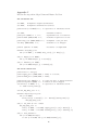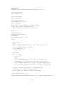
1
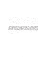
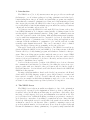
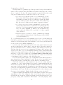
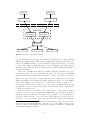
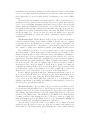
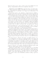
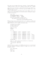
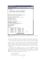
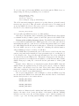
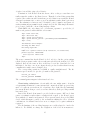
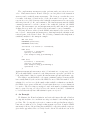
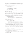
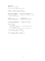
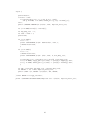
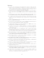
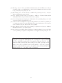
Kestrel: An Interface from Modeling Systems to the NEOS Server
Elizabeth D. Dolan
Industrial Engineering and Management Sciences Department, Northwestern University
Mathematics and Computer Science Division, Argonne National Laboratory
[email protected]
Robert Fourer
Industrial Engineering and Management Sciences Department, Northwestern University
[email protected]
Jean-Pierre Goux
Artelys S.A.
[email protected]
Todd S. Munson
Mathematics and Computer Science Division, Argonne National Laboratory
[email protected]
This work was supported by the Mathematical, Information, and Computational Sciences Division
subprogram of the Office of Advanced Scientific Computing, U.S. Department of Energy, under Contract W-31-109-Eng-38, and by the National Science Foundation Information Technology Research
initiative under grant CCR-0082807.
1
Abstract. The NEOS Server provides access via the Internet to a broad variety
of optimization software packages. Kestrel, a new interface to the NEOS Server,
extends the Server’s usefulness by permitting local programs rather than human
modelers to request optimization services and retrieve results. As a result, a locally
running modeling system can have much the same access to remote NEOS solvers as
to solvers installed locally; modelers can consider a wider variety of solvers, problems
may be solved more effectively, and new solver technologies may be disseminated
more rapidly.
Kestrel client programs have been implemented to support NEOS requests from
locally executing instances of the AMPL and GAMS modeling environments. Extensions to the client designs enable them to queue subproblems for execution and
later retrieval of results, making possible a limited form of parallel processing in
some circumstances. The creation of the Kestrel interface has also led the NEOS
Server to be enhanced with more flexible features for submitting binary files and for
tracking progress via the Web.
2
1. Introduction
The NEOS Server [7, 8, 9, 18], www-neos.mcs.anl.gov, provides access through
the Internet to over 45 software packages for solving optimization and related problems including linear, integer, stochastic, and semidefinite programs, unconstrained
and nonlinearly constrained optimization problems, and complementarity problems.
Since its inception in 1996, the NEOS Server has been progressively enhanced and
now readily handles 5,000–10,000 submissions per month from a variety of business,
educational, and scientific endeavors [10, 11].
Problems are sent to the NEOS Server via email, Web-based forms, or the socketbased NEOS Submission Tool. Output consists basically of a listing returned to the
user through the original submission interface. Using “print” commands, users can
control the form and content of the listing. Although this arrangement is satisfactory for small class assignments and for comparison of solvers, it offers little help
with the integration of optimization into broader modeling and application environments. Both the submission of optimization “jobs” and the retrieval of results
normally require human intervention. They can be automated only to a limited
degree through problem-specific programming on the part of the user.
This paper describes the new Kestrel interface to the NEOS Server and its application within the AMPL [13, 14] and GAMS [4, 5] modeling systems. A Kestrel
client is called by a locally running program, and results are returned to that program. Thus, a modeling system can have much the same access to remote NEOS
solvers as to solvers installed locally. As a result, the modeler can consider a wider
variety of solvers, problems may be solved more effectively, and new solver technologies may be disseminated more rapidly.
Section 2 briefly reviews the operation of the NEOS Server. Section 3 discusses
the communication and interface problems faced in calling the server from a program, together with our solutions to these problems as embodied in the design of
the Kestrel interface. Section 4 then describes the Kestrel clients for the AMPL and
GAMS modeling systems.
By using a paradigm similar to that described in [12], an extension to the Kestrel
client enables modeling language scripts to queue subproblems for execution and
later retrieval of results. Section 5 describes this and related features. Section
6 provides an example in which this mechanism is employed to solve a two-stage
stochastic location-transportation problem by Benders decomposition.
2. The NEOS Server
The NEOS Server is the most ambitious realization to date of the optimization
server idea [15]. Operated by the Optimization Technology Center of Argonne National Laboratory and Northwestern University, it represents a collaborative effort
involving over 40 designers, developers, and administrators around the world. The
project solicits solvers of all kinds, including ones that are proprietary to varying degrees (but whose owners have been willing to permit their use at no charge through
the server). Although the server’s location is fixed, the actual solvers can run on any
workstation connected to the Internet. Hence, available computing resources can
grow along with the number of solvers and users. New solvers are registered through
the same mechanisms as ordinary optimization job requests by using a standard and
3
documented procedure [9].
The large number of optimization problem types and solvers precludes standardization on any one input format. The NEOS Server instead allows any text or binary
files to be passed to a solver. The formats currently recognized fall into three main
categories determined largely by what the solvers are able to accept:
Low-level formats explicitly describe every constraint and objective.
They include MPS [23] for linear programs, sparse SDPA [16] for
semidefinite programs, SIF [6] for nonlinear programs, and SMPS
[1] for stochastic programs. Since these formats often result in large
files, the server recognizes several common compression schemes.
C or Fortran programs represent constraints and objectives by subroutines that evaluate the needed functions at a points specified by
the solver. For solvers requiring derivatives, automatic differentiation tools, such as ADIFOR [2], ADIC [3, 20], and ADOL-C [17],
can be run by the NEOS solver to generate code that computes
exact derivatives.
High-level algebraic formulations describe optimization problems in
concise, symbolic formats using modeling languages such as AMPL
[13, 14] and GAMS [4, 5].
To cope with this variety, the server maintains a data bank, a general framework
that enables optimization solvers and their individual needs to be recognized. Each
available solver has an entry in the data bank that records solver-specific information
provided by the solver’s NEOS administrator.
A solver’s entry in the data bank includes a list of the input formats it accepts
and the workstations on which it may be run, user help for its various interfaces,
and other information used to construct its listing on the NEOS Server Web site.
The data bank also stores a token configuration file listing a label and type (file,
check-box, text field, etc.) for each submission interface item, tokens (strings) that
delimit solver input, and the names of the files into which the delimited parts of the
input are to be placed. For example, the tokens BEGIN.MODEL and END.MODEL might
be associated with a neos.mod file. All of the input between these two tokens in a
job submission would be written to a file called neos.mod.
If a solver uses separate scripts to process submissions from different input formats, it must have a data bank entry for each. The size of the data bank is nevertheless kept reasonable; currently there are 108 entries for 46 distinct solvers.
Under this arrangement, each submission to the server is a single input file,
comprising one or more parts delimited by tokens. For email submissions the user
inserts tokens explicitly, while the Web and NEOS Submission Tool interfaces insert
appropriate tokens automatically. Consulting the data bank entry for the requested
solver, the server unpacks the input into files and chooses a workstation on which
the submission will be run. The files are then transmitted to the workstation, and
the remote solver is initiated. Further details of this process are given in [9].
Compressed input is automatically detected and expanded as part of the server’s
unpacking procedure. Line endings are then converted as necessary to account for
the different text conventions of Windows, Macintosh, and Unix systems. More complex preprocessing, such as automatic differentiation or modeling language trans4
lation, is performed as part of the solver activities after the problem is sent to a
workstation.
When the remote solver is executed, all text appearing on “standard output” is
passed back to the NEOS Server, which forwards it to the user through email, the
Web, or the NEOS Submission Tool as appropriate. The development of the Kestrel
interface has also led to a mechanism for viewing the intermediate output through
a Web browser, as we explain in the following section.
In 2001–2002, the NEOS Server typically received over a thousand submissions
each week, with peak loads of several thousand. In any system of this complexity, varied problems arise: machines go down, software crashes or terminates in
unexpected ways, and solvers run much longer than expected. The NEOS Server
developers have used this experience to implement refinements that improve reliability. Questions and comments from users are automatically logged and distributed
to a mailing list of Optimization Technology Center members and affiliates.
3. The Kestrel Interface
Effective use of optimization involves more than modeling and solving; the results
also need to be returned in a useful form. Whether the NEOS Server returns results
in a Web page, an email message, or a window of the NEOS Submission Tool,
a listing—a text file of problem statistics and results—is always returned. Some
modelers are content to look at the listing, while others either write their own
processing programs or cut and paste from the listing to standard software such as
spreadsheets.
Such listings are inconvenient when the results are to be manipulated by a program rather than directly by a human modeler. In particular, effective use of a
modeling environment requires that the results be returned in an appropriate format for that environment. The modeler then accesses and manipulates the results
through the environment’s user interface.
To support the needs of modeling environments, the NEOS Server thus requires
an additional method of access. The new Kestrel interface provides this access by
enabling modeling environments to send optimization problems to the server and
retrieve the results by means of a function call, without human intervention.
The design of the Kestrel interface (Figure 1) comprises new client and server
software and their interconnection via the CORBA standard. This section describes
the CORBA foundation for the Kestrel interface, the general features of the client
and server, and several changes to the NEOS Server—none major—necessitated by
the new link with the Kestrel server.
The CORBA foundation for the Kestrel interface. In the simplest terms,
a callable interface to the NEOS Server requires some mechanism for making function calls over the Internet. The local computer must be able to call a function
that actually runs on a remote computer with access to the NEOS Server. In an
object-oriented programming environment, this arrangement must extend to the
instantiation of objects and the invocation of their member functions.
Fortunately, standard “middleware” is readily available for this purpose. We
have decided to use the Object Management Group’s CORBA (www.corba.org)
5
AMPL Session
GAMS Session
AMPL Kestrel Client
GAMS Kestrel Client
CORBA Internet Interface
Kestrel Server
AMPL Kestrel
Solver Object
GAMS Kestrel
Solver Object
NEOS Server
Solver Workstation
Solver Workstation
Solver Workstation
Figure 1: Structure of the Kestrel interface.
[19], an established and well-supported standard.∗ In particular, we employ IONA’s
ORBACUS implementation (www.iona.com/products/orbacus_home.htm). Because the CORBA standard is widely available, Kestrel clients can be provided
for any of the numerous platforms supported by optimization modeling systems.
Initially, we have made the Kestrel clients available for Windows/Intel, Linux/Intel,
and Solaris/SPARC.
The heart of CORBA is its Interface Definition Language, in which a developer
specifies the interface the remote application presents to a local program. A CORBA
implementation then translates this specification to “stub” and “skeleton” files upon
which a developer builds the local program and remote application, respectively.
Although CORBA local programs and remote applications need not be programmed
in the same language, we have used C++ throughout. In the context of C++,
the stub and skeleton files contain code for the required CORBA functions and
declarations of the C++ classes and member functions that must be implemented
to make the interface work.
When the interface is completed and operational, a local program obtains a
reference to a remote object by supplying a CORBA Interoperable Object Reference,
which incorporates an Internet host name and port number, and an applicationspecific key that locates the object on the host. Methods invoked on the reference to
the remote object are executed on the remote machine. The result is an arrangement
∗
Competing technologies include DCOM, Microsoft’s Distributed Component Object Model
(www.microsoft.com/com/tech/DCOM.asp); Microsoft’s more recent .NET technology (www.
microsoft.com/net/); and DCE, the Open Software Foundation’s Distributed Computing Environment (www.opengroup.org/dce/).
6
in which the user can make seemingly local calls to functions defined on an actually
remote object. This design nicely parallels our objectives in creating a user interface
that behaves like a local solver while relying on submission to the remote NEOS
Server.
We now describe the workings of the Kestrel interface. The local and remote programs are referred to as the Kestrel client and Kestrel server, which share a Kestrel
solver object via CORBA. Essentially, the Kestrel server accepts connections with
Kestrel clients and instantiates Kestrel solver objects. The Kestrel solver objects
have member functions that format problem information from the client, pass it to
the NEOS Server, and later return the results to the client. The NEOS Server schedules the incoming “jobs” on solver workstations, where the NEOS solvers—typically
executable scripts that set options and call the optimization software packages—
actually reside.
The Kestrel client. When a Kestrel client is executed on the local machine, a
connection with the Kestrel server is first established. Because only one computer
is currently used for the Kestrel server, a static object reference is built into the
available Kestrel clients. We could switch to a more flexible setup, however, if it
were desirable to change server machines regularly or have multiple Kestrel servers.
The optimization problem to be solved is then located on the local machine
and other settings or information required by the intended solver is gathered. The
Kestrel client then makes a call to the Kestrel server via CORBA to instantiate a
new Kestrel solver object. Several member functions of the Kestrel solver object are
then invoked. The first submits the optimization problem and other information.
This call returns via output parameters a NEOS job number and password, which
the client can pass to the user. As explained later in this section, the job number
and password can be used, for example, to check on the job status. A blocking call
requesting the results from the remote solver is then issued. Upon return, the client
performs any processing of the results needed locally. A final call to destroy the
Kestrel solver object is then issued to free resources on the Kestrel server.
Because different applications may have different information they pass to remote solvers, distinct Kestrel solver objects are needed. In the implementation, the
Kestrel solver is a base class. When the Kestrel client calls the server to obtain a
solver object, it specifies which child class of the base is to be instantiated. The
differing requirements of the AMPL and GAMS modeling languages, described in
the next section, are handled in this way.
The Kestrel solver. We now turn to the process whereby the Kestrel solver
object interacts with the NEOS Server. The Kestrel solver first concatenates the
submission data received from the client, inserting the appropriate token delimiters.
The resulting data is then written to a file with a unique name in the spool directory
specified by the NEOS Server. The initializer for the NEOS Server then assigns a
job number and moves the submission to the job directory for later processing. The
same mechanism is used by the NEOS Server to locate and initialize submissions
received from the Web and NEOS Submission Tool interfaces.
Once the Kestrel solver has obtained a job number, the job password is then
acquired from a file in the job directory. Both the job number and password are
then returned to the Kestrel client. This submission procedure requires that the
7
Kestrel solver have access to the spool and job directories the NEOS Server uses
when processing submissions. Hence the two must share a file system.
Implications for the NEOS Server. The introduction of the Kestrel interface did not require major changes to the NEOS Server. The unavoidable changes
were straightforward. Several turned out to support other enhancements to the
NEOS Server.
A previously described, each combination of a Kestrel client type (AMPL or
GAMS) and solver has an entry in the data bank. Thus, the files received through
the Kestrel interface can be properly recognized and processed by the NEOS Server.
An early implementation of the Kestrel procedure for retrieving results simply
checked every few seconds until a results file was found in the job directory. We
quickly discovered that file locking mechanisms are much more efficient in terms of
CPU load. The NEOS Server now creates a file in the job directory and obtains an
exclusive lock on it. The lock is released when the results are ready. The Kestrel
solver performs a blocking call (whose cost is negligible compared with multiple
system calls) to gain a lock on the same file. When this call returns, the Kestrel
solver then knows the results are ready and can proceed to parse the result file on
predefined tokens for return to the Kestrel client. Obviously, this more efficient
retrieval mechanism relies on a file system that supports file locking correctly. We
have found it convenient to run both the Kestrel and NEOS Servers on one machine,
and to use the local hard drive to encourage file system efficiency.
Because the Kestrel interface must deal with input from programs, instead of
submissions from human modelers, it must be able to handle both binary and text
input. Since the NEOS Server already detects and handles compressed file formats,
which are special cases of binary inputs, the only change necessary to accept arbitrary binary input was to tag it so that the server does not apply its conversion of
apparent line endings. This feature has subsequently been used to extend the flexibility of other server interfaces. For example, some solvers on the NEOS Server now
read gzip-compressed file input directly, and others now accept MATLAB binary
files.
The Kestrel interface, unlike the Web interface and NEOS Submission Tool,
does not maintain an open connection for piping intermediate solver output back
to the user. Therefore, to provide Kestrel users with some way to check that their
longer-running jobs actually were progressing, we added a page (Figure 2) to the
server Web site enabling users to request intermediate results by typing in the job
number and job password previously reported to the Kestrel client and clicking on
the “View Intermediate Results” button. The client can display the job number and
password for the user or can construct a URL that automatically loads the result
request page with the number and password fields already filled.
This page was easily adapted to provide other useful services. A “View Final
Results” button was added to allow for retrieval of results from completed jobs for as
long as the NEOS Server keeps the results on file (currently a few days). This feature
was appreciated by Web users who occasionally lost Internet connectivity and still
wanted to retrieve their results through a Web browser. A “View Job Queues”
button was also added to show all submissions currently executing or queued for
execution.
8
Figure 2: The NEOS Server’s Web page for requesting solver output views.
4. Kestrel Clients for Modeling Languages
Optimization modeling languages [21] are widely used for the kinds of prototyping and testing that are a major application of the NEOS Server because of
their convenience and power. In fact, the email, Web, and NEOS Submission Tool
interfaces have accepted modeling language input for some years. Currently, over
two-thirds of the submissions received by the NEOS Server are in the AMPL and
GAMS languages.
Some of the advantages of a modeling language are lost, however, when it is
merely used as in input format to the NEOS Server. In such cases, a language
translator is first invoked on the remote solver workstation to convert the submission
into a format suitable for input to the optimization software. For security reasons,
file writing and other local features are turned off when the translator is run. In
9
the end, only a listing is returned and any interactivity the modeling system might
provide as a locally installed system is lost in the NEOS Server environment.
These difficulties can be circumvented by taking advantage of the Kestrel interface to the NEOS Server. All of the interactivity and other features of the modeling
system remain available under this arrangement. Because the security restrictions
do not apply during local operation, users can access the file system and related
utilities—such as tools for obtaining data from spreadsheets or databases—when
working with a model. After the remote solver has finished, the results are returned
in a form suitable for further local processing by the modeling system.
Moving the language translation to the local machine also results in a reduction
in the load on NEOS solver workstations. Job submissions to the NEOS Server
that result in nothing more than syntax error reports are reduced. Further, model
errors are reported much more quickly because the time a model translator requires
to detect and report an error is much less than the overhead of passing the model
through the NEOS Server to a remote copy of the translator.
In the remainder of this section, we describe the basic modeling language clients.
We first show how they are used and then comment on significant aspects of their
design.
Using the modeling language clients. Both GAMS and AMPL employ temporary files for the exchange of information with a solver. Thus, from the modeling
system point of view, the invocation of a solver has three general steps:
Write a representation of the current problem instance to one or
more files.
Locate the specified solver, execute it with appropriate options, and
wait for it to write one or more solution files.
Read the solution files and resume processing.
The Kestrel interface replaces the local solver with a Kestrel client. The fact that
the Kestrel interface is used to solve the problem instance via the NEOS Server,
rather than directly via some locally installed solver, makes little difference to the
GAMS or AMPL system.
As an example, the AMPL commands for solving the steel.mod sample problem
(www.ampl.com/BOOK/EXAMPLES/steel.mod) by using a locally installed copy of the
LOQO solver [24] are as follows:
ampl:
ampl:
ampl:
ampl:
ampl:
model steel.mod;
data steel.dat;
option solver loqo;
option loqo_options 'mindeg sigfig=8 outlev=1';
solve;
The corresponding commands to solve the same problem by using LOQO through
the NEOS Server are much the same:
ampl:
ampl:
ampl:
ampl:
ampl:
ampl:
model steel.mod;
data steel.dat;
option solver kestrel;
option kestrel_options 'solver=loqo';
option loqo_options 'mindeg sigfig=8 outlev=1';
solve;
10
The solver option is changed from loqo to kestrel, so that the AMPL solve
command now passes control to the local Kestrel client program. Also a command
setting kestrel_options is added so that the Kestrel interface knows which remote
NEOS solver has been requested. In all other respects, the AMPL session to this
point is the same as before.
As soon as the current problem instance has been successfully conveyed to the
NEOS Server, the client displays some useful information, including the assigned
job number and password:
ampl: solve;
Job has been submitted to Kestrel
Kestrel/NEOS Job number
: 115407
Kestrel/NEOS Job password : VPZKESEV
Check the following URL for progress report :
http://www-neos.mcs.anl.gov/neos/neos-cgi/
check-status.cgi?job=151480&pass=lzjeVJPQ
Further messages appear only when the remote solve completes, at which point
everything written to standard output by the remote solver is relayed back via the
NEOS and Kestrel Servers for display by the Kestrel client:
Intermediate Solver Output:
Checking the AMPL files
Executing algorithm...
LOQO 6.02: mindeg
sigfig=8
outlev=1
It’s a QP.
1
1.919905e+05
2
2.059650e+05
3
2.171855e+05
4
1.885680e+05
5
1.918103e+05
6
1.919905e+05
7
1.919995e+05
8
1.920000e+05
9
1.920000e+05
Finished call
3.4e+00
2.9e-01
2.2e-01
1.2e-14
1.6e-14
3.9e-15
9.6e-15
2.7e-14
5.6e-15
1.004000e+06
3.499774e+05
2.539125e+05
2.005521e+05
1.924522e+05
1.920226e+05
1.920011e+05
1.920001e+05
1.920000e+05
1.0e+00
1.9e-01
7.5e-04
5.5e-06
3.0e-07
1.5e-08
7.5e-10
3.7e-11
1.9e-12
1
1
2
4
5
6
8
PF
PF
PF
PF
PF
PF
DF
DF
DF
DF
DF
LOQO 6.02: optimal solution (9 QP iterations, 17 evaluations)
primal objective 191999.9988
dual objective 192000.0028
ampl:
All solution values are returned to the AMPL system and can be accessed through
subsequent commands. The display command, for example, can be used to browse
through the solution:
ampl: display Make;
Make [*] :=
bands 6000
coils 1400
;
11
Figure 3: The NEOS Server’s Web page for intermediate output of a solver, scrolled down
to the bottom.
The state of the AMPL system is in fact exactly the same at this point (except for
the setting of the solver option) as it would have been had the solver run locally.
To view intermediate output, the user pastes the given Web address (actually
displayed all on one line) into any Web browser window, bringing up the NEOS
Server’s results pages (shown previously in Figure 2). Clicking “View Intermediate
Results” brings up a window (Figure 3) showing what the solver has written to
standard output so far along with a few buttons providing convenient ways to refresh
the display.
The arrangement for GAMS is analogous. To run the GAMSLIB trnsport
model (www.gams.com/modlib/libhtml/trnsport.htm), for instance, the command
gams trnsport is issued. The GAMS system then looks for additional commands
within the file trnsport.gms. To solve the problem by using a local copy of the
MINOS solver, the relevant commands are as follows:
model transport /all/;
option lp = minos;
solve transport using lp minimizing z;
12
To solve the same problem using MINOS remotely through the NEOS Server, we
simply change the linear programming solver to kestrel:
model transport /all/;
transport.optfile = 1;
option lp = kestrel;
solve transport using lp minimizing z;
The added statement transport.optfile = 1 specifies that an options file, named
kestrel.opt, is provided. This options file conveys the remote solver name as well
as any algorithmic directives for the remote solver. For example, to use MINOS as
the remote solver, kestrel.opt includes the line
kestrel_solver minos
and optionally any MINOS directives on additional lines.
After the problem instance has been submitted, the GAMS Kestrel client displays
a confirmation with job number, password, and URL, just as for the AMPL client.
Design of the modeling language clients. The AMPL and GAMS interfaces
to solvers differ in significant ways. AMPL passes the solver name and directives
individually through a procedure modeled on Unix environment variables, for example, while GAMS uses the file system for this purpose. When the solver has finished
its work, AMPL expects to receive a single file containing all result information,
whereas GAMS provides for a variety of result files.
The GAMS Kestrel client must also remove all references to the license and other
system components in the internal problem representation prior to sending the job
to the Kestrel solver. Proper licenses and information for the solver workstation
are inserted later by the NEOS solver. This practice helps preserve the integrity of
the user system by not sending license information over the Internet unnecessarily.
GAMS client preprocessing also converts all absolute path names to relative path
names.
In light of these differences, we implement separate Kestrel AMPL client and
GAMS clients. As explained in the preceding section, the two clients are distinct
child classes of the Kestrel solver base class. These child classes define member
functions for sending problems and retrieving results that are appropriately tailored
to the needs of their corresponding languages.
Also as previously indicated, each combination of client and NEOS solver has
its own entry in the NEOS Server data bank. Hence the introduction of the Kestrel
interface has given rise to new entries such as
KESTREL_AMPL:MINOS
KESTREL_AMPL:SNOPT
···
KESTREL_GAMS:MINOS
KESTREL_GAMS:SNOPT
···
These entries are distinct from the existing data bank entries for modeling language
input to the same solvers because the nature of the input is different. Existing
interfaces send the server the modeling language source, which is translated by
a remote copy of the modeling system running on the same workstation as the
13
solver. The Kestrel interface provides the server with the intermediate text or
binary representation of the problem instance, the result of a translation already
performed by a local installation of the modeling system.
When a solver called through the Kestrel interface finishes, it must return the
listing file and other files expected by the modeling system. To make this possible,
the NEOS solver concatenates the necessary output into one token-delimited file that
is passed back through the NEOS Server to the Kestrel solver that invoked it. As in
the case of the inputs, the outputs for AMPL and GAMS are substantially different.
Hence the delimiting tokens are defined differently in the AMPL and GAMS child
classes of the Kestrel solver. In either case, however, the Kestrel solver uses the
tokens to break the solver output into appropriate files that can be processed by the
modeling environment. The Kestrel client completes its run by displaying the listing
file, creating appropriate local files for returned information, deallocating memory
both locally and at the Kestrel server, and returning control to the modeling system.
5. Submission and Retrieval from Modeling Language Clients
We have assumed in the previous examples that the Kestrel client remains active
until results from the remote solver have been returned. This arrangement works
well for a user whose number of submissions and solution time per submission is
manageable. In other circumstances, however, we have found that the Kestrel facilities can be made considerably more useful and fault-tolerant by allowing job
submission and retrieval to be requested separately by the user. Should a failure
occur on the local machine or in the Kestrel server while a problem is being solved
on a remote workstation, the user can repeat their result request at a later time after
the failure has been corrected. The user may also deliberately terminate the Kestrel
client and then perform other steps before requesting the results of a solve that is
expected to take a long time. For example, in some AMPL or GAMS environments
the user can deliberately “break” out of a client session by typing control-C. The
user’s interim steps may even include the submission of other problems through the
Kestrel interface. By automating this possibility, we have been able to go beyond
our original design goals by providing a rudimentary form of parallel processing.
In this section, we first describe two simple Kestrel extensions: one for retrieving
results from submissions that have become disconnected, and the other for requesting cancellation of a job. We then discuss the enhanced utilities for managing
multiple submissions through the Kestrel interface.
Retrieving disconnected submissions. Inevitably some Kestrel client processes terminate prematurely. If the termination of the Kestrel client occurs after
the problem-submission call has completed, however, then further operations on the
NEOS Server side are not affected. In particular, the NEOS Server still queues the
problem and solves it on a remote workstation.
Since the Web pages of intermediate results are generated by the NEOS Server
independently of how the submission was made, termination of the Kestrel client
does not prevent such results from being viewed through a Web interface like the
one shown in Figure 3. Following completion of the NEOS solver, the intermediate
results listing can be viewed through the same Web interface for as long as the
NEOS Server keeps it on file—currently a few days. This information is sometimes
14
of value for troubleshooting solver behavior.
Termination of the Kestrel client also has no effect on the processes that eventually return the results to the Kestrel server. Thus the local modeling system that
requested the results can still obtain them, provided that it can restart the Kestrel
client and can instruct it to retrieve a previous submission rather than begin a new
one. The submission of interest can be identified by its job number and password,
such as 151480 and lzjeVJPQ from the example in Section 4. This simple alternative
proved easy to build into our modeling language clients.
With AMPL, the only change is to set kestrel_options to provide the job
number and password rather than the solver name:
ampl:
ampl:
ampl:
ampl:
ampl:
model steel.mod;
data steel.dat;
option solver kestrel;
option kestrel_options 'job=115407 password=VPZKESEV';
solve;
Intermediate Solver Output:
Checking the AMPL files
Executing algorithm...
···
LOQO 6.02: optimal solution (9 QP iterations, 17 evaluations)
primal objective 191999.9988
dual objective 192000.0028
ampl:
The solve command invokes the Kestrel “solver” as before, but the option settings
tell the client program to make only a result-retrieval call for the indicated job. The
displayed lines are the same as they would have been if the client had not been
interrupted, but they come from output already produced rather than from any
communication with a remote LOQO solver.
The corresponding extension for GAMS is equally straightforward. The file
kestrel.opt is extended to give the job number and password,
kestrel_job 115407
kestrel_password VPZKESEV
The command gams trnsport is then issued as before.
Terminating submissions. Occasionally, the user might want to abandon
a long-running submission because intermediate output shows little progress being
made or because an error in the model or data has come to light. Merely terminating
the current Kestrel client process does not have this effect, as the preceding remarks
have made clear.
Instead the Kestrel client must be provided with a separate “kill” mode that
passes a termination rather than a result-retrieval request to the Kestrel server
along with the job number and password. The request is passed along to the NEOS
Server, which attempts to pass it to the workstation running the solver. (Certain
combinations of workstation and solver are not configured to recognize termination
requests.)
The mechanisms of the modeling languages are readily adapted to invoke the
kill mode. For GAMS, we change the designation of the solver from kestrel to
15
kestrelkil (with one final l due to a GAMS limitation of 10-characters per solver
name):
model transport /all/;
transport.optfile = 1;
option lp = kestrelkil;
solve transport using lp minimizing z;
The job number and password are placed into the kestrel.opt file as before.
In the case of AMPL, kestrel_options is set as above, and a command script
kestrelkill is invoked:
ampl: option kestrel_options 'job=115407 password=VPZKESEV';
ampl: commands kestrelkill;
The script resides in a file named kestrelkill in the current working directory
that has just one line,
shell 'kestrel kill kestrel';
that runs the quoted Kestrel client command. We might have preferred to pass all
of the information to the client through kestrel_options, by recognizing a setting
of, say, 'kill job=115407 password=VPZKESEV' followed by a solve command to
invoke the Kestrel “solver” as before. AMPL’s solve is not convenient for this
purpose, however, because it refuses to invoke a solver until a model and data have
been translated into a current problem instance. The kestrelkill script can be
run even when no model and data have yet been read in the current session.
Managing submissions and retrievals. Most optimization modeling systems provide a way of defining iterative schemes that solve one or more models
repeatedly. Common examples include sensitivity analysis, cross validation, decomposition, and row or column generation.
For these purposes the modeling language is extended to provide typical programming statements—such as assignments, tests, and loops—that use the same
indexing and expressions as the language’s model declarations. Programs, or scripts,
using the new statements also have access to any of the commands already available for solving and manipulating problem instances. Thus, in particular, all of the
commands we have shown for use of the Kestrel interface can be employed within a
script, allowing scripts to do some processing on the local computer while sending
optimization runs to NEOS solvers.
Many iterative schemes involve, in whole or part, the solution of successive collections of similar but independent subproblems. Since the NEOS Server typically
has multiple workstations listed to run the required solver, we might prefer to send
batches of subproblems to the NEOS Server, rather than submitting each subproblem and waiting for its solution before submitting the next. The effect is an elementary form of parallel processing that uses the NEOS Server’s scheduler to manage
the parallelism.
Because the Kestrel client’s problem-submission calls are separate from its resultretrieval calls, we can adapt the approach that Ferris and Munson [12] employed
in their scheme for controlling Condor-based workstation pools from modelinglanguage scripts. Basically, the “solve” command can be replaced by separate “sub-
16
mit” and “retrieve” scripts or commands. Any number of submission requests are
permitted, with retrievals taking place in the same order.
In our AMPL realization of this approach, the statement commands kestrelsub
runs a short script that submits the current problem instance. The statement
commands kestrelret runs another short script that waits for the completion of
the earliest-submitted problem that is still active. For example, a simple sensitivityanalysis loop for steel.mod that steps the value of parameter avail at each pass
for {a in 37..42} {
let avail := a;
solve;
let avail_obj[a] := Total_Profit;
}
could be replaced by a pair of loops, one to make submissions for the sequence of
parameter values and one that retrieves the results:
for {a in 37..42} {
let avail := a;
commands kestrelsub;
}
for {a in 37..42} {
let avail := a;
commands kestrelret;
let avail_obj[a] := Total_Profit;
}
By indexing over the same set in both loops, this script ensures that retrieval of
problem results occurs in the same order as problem submission.
The AMPL Kestrel client implements this behavior by use of a single temporary file. Each kestrelsub causes the resulting job number and password for the
submission to be written to the end of the file. The kestrelret command requests
results for the file’s first entry, which is then deleted. The kestrelsub script is just
three lines:
option ampl_id (_pid);
write bkestproblem;
shell 'kestrel submit kestproblem';
as is the kestrelret script:
option ampl_id (_pid);
shell 'kestrel retrieve kestresult';
solution kestresult.sol;
The first line serves only to insure that all invocations of the client refer to the same
temporary file, whose name is constructed from the parameter _pid that AMPL
predefines to equal the process ID of the current AMPL session.
In kestrelsub the write command generates a binary problem instance in a
file kestproblem.nl. Then the shell command starts a Kestrel client process with
the instruction submit and the problem file name. The client process reads the file,
submits it to the server, adds the resulting job number and password to the job file,
and then terminates without waiting for a result.
17
The complementary kestrelret script performs analogous actions in reverse
order. First shell starts a Kestrel client process but passes it the instruction
retrieve and a result file name kestresult. The client process asks the server
for results of the first job listed in the job file, then waits for a response. Once a
response is received, the client saves the results file as kestresult.sol, removes the
first entry from the job file, and terminates. The final statement runs the AMPL
command solution to read the contents of the results file back into the AMPL
system. The kestresult.sol and kestproblem.nl files still exist in the current
working directory at the end of such a session and must be removed manually.
The same effects are achieved in the GAMS environment by the creation of two
new “solvers”—kestrelsub and kestrelret—that implement the submission and
retrieval parts of the Kestrel client. The following commands then implement a
sensitivity analysis for the trnsport example:
SET iter /1*5/;
PARAMETER optval(iter);
PARAMETER avail(iter);
avail(iter) = a(’seattle’) + 10*ord(iter);
LOOP (iter,
a(’seattle’) = avail(iter);
option lp = kestrelsub;
solve transport using lp minimizing z;
);
LOOP (iter,
a(’seattle’) = avail(iter);
option lp = kestrelret;
solve transport using lp minimizing z;
optval(iter) = z.l;
);
Again kestrelsub and kestrelret write job information to a temporary job file.
We break with GAMS convention by also using kestrel.opt as the options file for
both, rather than looking for separate files kestrelsub.opt and kestrelret.opt.
The ability to use this facility to solve many optimization subproblems in parallel
is necessarily limited by the extent of the NEOS resources. When the number of jobs
submitted for a solver exceeds the number that available workstations can handle,
the NEOS Server queues additional jobs and starts them as soon as workstations
become free. The Server imposes an upper bound on the number of submissions that
may be queued for any one solver, however; the current bound is 15. Submissions
to a solver that already has a full submission queue are rejected.
6. An Example
We illustrate the Kestrel submission and retrieval features through a Benders
decomposition scheme for a nonlinear two-stage stochastic location-transportation
problem. The decomposition gives rise to numerous independent linear subproblems, whose results are fed to a single nonlinear master problem. Complete AMPL
statements of the models and data plus an AMPL decomposition-scheme script are
given in the appendixes. Here we briefly describe the model and then focus on the
18
parts of the script that use Kestrel features.
The model. We consider the problem of deciding how much warehouse capacity
to build at specified locations, for the purpose of satisfying uncertain demands at
specified retail stores. Because of the lead time required to build warehouses, the
capacities must be decided before the demands are known, but the amounts shipped
can be tailored to the actual demands. To keep our presentation no more complicated than necessary for demonstrating the Kestrel submission tools, we confine our
example to a single commodity and a single period. We allow for multiple demand
scenarios, however, and seek the warehouse construction plan that minimizes the
expected value of total distribution costs.
In the AMPL terminology, the model is founded on sets WHSE of potential warehouse locations, STOR of stores, and SCEN of scenarios. For each warehouse location
i, we must decide how many units Build[i] of capacity to construct, at a cost of
build_cost[i] * Build[i] / (1 - Build[i]/build_limit[i])
Thus the cost is a convex increasing function of the capacity built, with an upper
limit of build_limit[i] (since the cost goes to infinity as Build[i] approaches
that value). Total construction cost is the sum of these costs over all i in WHSE.
Each scenario s occurs with probability prob[s] and requires the shipment of
an amount demand[j,s] to each store j. For each combination of a warehouse i
and a store j under scenario s we must decide how many units Ship[i,j,s] to
ship, at a linear cost of ship_cost[i,j] * Ship[i,j,s]. The total shipping cost
for scenario s is the sum of this expression over all combinations of i and j, and
hence the expected value of the total shipping cost is given by
prob[s] * sum {i in WHSE, j in STOR} ship_cost[i,j] * Ship[i,j,s]
summed over all s in SCEN.
The overall cost to be minimized is given by adding together the sums of the two
expressions above. Constraints at the warehouses say that the total shipped out of
warehouse i in any scenario s cannot exceed the capacity previously built at i:
sum {j in STOR} Ship[i,j,s] <= Build[i];
Constraints at the stores say that the total shipped into each store j in any scenario
s must equal j’s demand in that scenario:
sum {i in WHSE} Ship[i,j,s] = demand[j,s];
The complete AMPL model can be seen in Appendix A, and a sample of data for
it in Appendix B.
The master problem and subproblems. Fixing the relatively small subset
of Build[i] variables in our model disconnects it into a collection of independent
linear programs, one for each scenario. We can write a single AMPL subproblem
model by defining a subproblem-valued parameter
param S symbolic in SCEN;
and dropping the subproblem index from the shipment variables. We fix the con-
19
struction variables at values build[i] and drop the now-fixed production costs from
the objective. We can also omit the scenario probability factor from the objective,
since its presence serves only to scale the optimal objective and dual values. What
remains is a pure transportation problem:
minimize Scen_Ship_Cost:
sum {i in WHSE, j in STOR} ship_cost[i,j] * Ship[i,j];
subj to Supply {i in WHSE}:
sum {j in STOR} Ship[i,j] <= build[i];
subj to Demand {j in STOR}:
sum {i in WHSE} Ship[i,j] = demand[j,S];
Any solver for minimum-cost network flows, or for linear programming generally,
can be applied to this problem.
As the solution of the subproblems proceeds, the optimal dual values prob[S] *
Supply[i].dual and prob[S] * Demand[j].dual are saved in parameters denoted
supply_price[i,s,nCUT] and demand_price[i,s,nCUT], with nCUT representing
the number of master-problem constraints or “cuts” generated so far—one per pass
of the decomposition procedure. These dual values are the only information from
the subproblems that are passed back to the master problem, whose objective is
minimize Expected_Total_Cost:
sum {i in WHSE}
build_cost[i] * Build[i] / (1 - Build[i]/build_limit[i])
+ Max_Exp_Ship_Cost;
with the variable Max_Exp_Ship_Cost—standing in for the shipping cost part of the
objective—constrained by the cuts:
subj to Cut_Defn {k in 1..nCUT}:
Max_Exp_Ship_Cost >=
sum {i in WHSE, s in SCEN} supply_price[i,s,k] * Build[i] +
sum {j in STOR, s in SCEN} demand_price[j,s,k] * demand[j,s];
The complete AMPL statements of the master problem and subproblem are given
in Appendix C.
The Benders master problem can be shown to provide a lower bound on the true
objective value, while the subproblems jointly provide a feasible solution that gives
an upper bound. The “gap” between these bounds can thus be used as a criterion
for deciding when to stop the decomposition procedure. For this example the gap
can be computed as
Exp_Ship_Cost - Max_Exp_Ship_Cost
where Exp_Ship_Cost is the sum of the subproblem objective values prob[S] *
Scen_Ship_Cost and Max_Exp_Ship_Cost is the stand-in for the shipping costs in
the most recently solved master problem (as seen above).
The decomposition scheme. With the variables, objectives, and constraints
set up as we have described, AMPL can define the master problem and subproblems
by the following statements:
20
problem Sub: Ship, Scen_Ship_Cost, Supply, Demand;
option solver afortmp;
problem Master: Build, Max_Exp_Ship_Cost,
Expected_Total_Cost, Cut_Defn, Feas_Guarantee;
option solver knitro;
The option solver settings following the problem declarations are recorded as part
of the problem environment, so that, in this case, the nonlinear solver knitro is used
in solving the master problem, while the linear programming solver afortmp is used
for the subproblems.
The heart of the Benders procedure is an AMPL loop that has the following
structure:
repeat {
problem Master;
solve;
let {i in WHSE} build[i] := Build[i];
let Exp_Ship_Cost := 0;
let nCUT := nCUT + 1;
problem Sub;
for {s in SCEN} {
/* process subproblem s here */
};
let GAP := min (GAP, Exp_Ship_Cost - Max_Exp_Ship_Cost);
let RELGAP := 100 * GAP / Expected_Total_Cost;
} until RELGAP <= relgap_tolerance;
Ordinarily the inner for loop would be written as
for {s in SCEN} {
let S := s;
solve;
let Exp_Ship_Cost := Exp_Ship_Cost + prob[S] * Scen_Ship_Cost;
let {i in WHSE}
supply_price[i,s,nCUT] := prob[S] * Supply[i].dual;
let {j in STOR}
demand_price[j,s,nCUT] := prob[S] * Demand[j].dual;
}
The complete script for Benders decomposition can be seen in Appendix D.
The script’s inner loop is where the Kestrel submission and retrieval facilities
can make a difference, because the subproblems are all independent linear programs.
Our revised script sets kestrel as the “solver” and identifies the actual solvers in
kestrel_options:
option solver kestrel;
problem Sub: Ship, Scen_Ship_Cost, Supply, Demand;
option kestrel_options 'solver=afortmp';
problem Master: Build, Max_Exp_Ship_Cost,
Expected_Total_Cost, Cut_Defn, Feas_Guarantee;
option kestrel_options 'solver=knitro';
21
We can break the subproblem processing into two loops, one that submits all the
subproblems
for {s in SCEN} {
let S := s;
commands kestrelsub;
}
followed by one that retrieves all the corresponding results:
for {s in SCEN} {
let S := s;
commands kestrelret;
let Exp_Ship_Cost := Exp_Ship_Cost + prob[S] * Scen_Ship_Cost;
let {i in ORIG}
supply_price[i,s,nCUT] := prob[S] * Supply[i].dual;
let {j in DEST}
demand_price[j,s,nCUT] := prob[S] * Demand[j].dual;
}
The complete revised script is shown in Appendix E.
This script’s first loop goes quickly, as it only submits all the subproblems. The
second loop is the same as before but with commands kestrelret replacing solve.
It must retrieve subproblems’ results in the order of submission, so some results may
sit on the Kestrel server waiting their turn to be retrieved. This need not create any
great inefficiency in our example, however, because the decomposition procedure
waits for all of the subproblems to be solved before going on to the next master
problem anyway. Other iterative schemes that generate numerous subproblems have
a similar property. (A more sophisticated Kestrel interface would be necessary,
however, to deal with “asynchronous” decomposition schemes [22] that may solve a
new master problem before all of the relevant subproblems have been received.)
When our script is run with the very small sample data file of Appendix B, the
overhead of submitting and retrieving Kestrel jobs dominates the total elapsed time.
For harder subproblems, however, we expect the network overhead will mostly overlap with the problem solving and will be small compared with the actual execution
times of the solvers. Any remaining network overhead will represent a price that
users are willing to pay in order to avoid the difficulties of setting up multiple solvers
on multiple local machines.
7. Further Directions
We have shown that a callable interface to the NEOS Server—the ability to solve
optimization problems through the NEOS Server without manual intervention—
can be implemented for any optimization environment that makes calls to separate solvers. Our initial effort with the Kestrel interface has focused on GAMS
and AMPL, but similar arrangements could readily be made for other optimization
modeling languages.
The Kestrel interface has also proved to have related uses we did not anticipate.
For example, the kind of parallelism described in Sections 5 and 6 takes advantage
of features originally conceived to provide fault tolerance in the event of a broken
connection between the client and server.
22
The availability of the Kestrel interface has also opened up the possibility of
implementing new services on the NEOS Server that exploit multiple resources.
As an example, a new GAMS/AMPL solver on the NEOS Server takes a GAMS
model as input, translates it into a scalar (unindexed) AMPL model on one server
workstation, and then solves it using the requested AMPL solver on a different
workstation. The implementation of this arrangement employs the Kestrel interface
to call the AMPL solver and obtain the results, which are then translated back
to the form GAMS expects. In this way, GAMS users can have access to all the
Kestrel-enabled AMPL solvers on the NEOS Server.
While we have concentrated on general-purpose environments based on modeling
languages, the same approach can also be used to make NEOS solvers available to
systems or front-ends that are specialized for particular applications. We expect
this to open up further unanticipated uses for the Kestrel interface.
23
Appendix A
AMPL Model for a Nonlinear
Two-Stage Stochastic Transportation Problem
set WHSE;
set STOR;
# shipment origins (warehouses)
# shipment destinations (stores)
param build_cost {WHSE} > 0;
param build_limit {WHSE} > 0;
var Build {i in WHSE} >= 0,
<= .9999 * build_limit[i];
# costs per unit to build warehouse
# limits on units shipped
# capacities of warehouses to be built
set SCEN;
param prob {SCEN} >= 0, <= 1;
param demand {STOR,SCEN} >= 0;
param ship_cost {WHSE,STOR} >= 0;
var Ship {WHSE,STOR,SCEN} >= 0;
# demand scenarios
# probabilities of scenarios
# amounts required at stores
# shipment costs per unit
# amounts to be shipped
minimize Total_Cost:
sum {i in WHSE}
build_cost[i] * Build[i] / (1 - Build[i]/build_limit[i]) +
sum {s in SCEN} prob[s] *
sum {i in WHSE, j in STOR} ship_cost[i,j] * Ship[i,j,s];
subj to Supply {i in WHSE, s in SCEN}:
sum {j in STOR} Ship[i,j,s] <= Build[i];
subj to Demand {j in STOR, s in SCEN}:
sum {i in WHSE} Ship[i,j,s] = demand[j,s];
24
Appendix B
AMPL Data
param: WHSE: build_limit :=
1 100000
6 80000
11 100000
2 80000
7 60000
12 80000
3 80000
8 80000
13 80000
4 60000
9 80000
14 60000
5 80000
10 80000
15 80000
param build_cost
16
17
18
19
20
60000
60000
80000
80000
80000
21
22
23
24
25
60000
80000
60000
60000
80000 ;
default 2 ;
param: SCEN: prob :=
low
0.5
mid
0.3
high
0.2 ;
set STOR :=
A3 A6 A8 A9 B2 B4 ;
param demand:
A3
A6
A8
A9
B2
B4
low
10000
9000
11000
10000
18000
24500
param ship_cost:
A3
A6
1
73.78
14.76
2
60.28
20.92
3
58.18
21.64
4
50.37
21.74
5
42.73
35.19
6
44.62
39.21
7
49.31
51.72
8
50.79
59.25
9
51.93
72.13
10
65.90
13.07
11
50.79
9.99
12
47.51
12.95
13
39.36
19.01
14
33.55
30.16
15
34.17
40.46
16
41.68
53.03
17
42.75
62.94
18
46.46
71.17
19
56.83
8.84
20
46.21
2.92
21
41.67
11.69
22
25.57
17.59
23
28.16
29.39
24
26.97
41.62
25
34.24
54.09
mid
12000
12000
14000
13500
25000
29000
A8
86.82
76.43
69.84
61.49
44.11
44.44
36.27
22.53
21.66
79.59
67.83
59.57
56.39
40.66
40.23
22.56
18.58
17.17
83.99
68.94
61.05
54.93
38.64
29.72
22.13
high :=
15000
14000
27500
15500
28000
39000 ;
A9
91.19
83.99
72.39
65.72
58.08
48.32
42.96
33.22
29.39
86.07
78.81
67.71
62.37
48.50
47.10
30.89
27.02
21.16
91.88
76.86
70.06
57.07
46.48
40.61
28.43
25
B2
51.03
58.84
61.64
60.48
65.76
76.12
84.52
94.30
93.52
46.83
49.34
51.13
57.25
60.83
66.22
77.22
80.36
91.65
41.38
38.89
43.24
44.93
50.16
59.56
69.68
B4 :=
76.49
68.86
58.39
56.68
55.51
51.17
49.61
49.66
49.63
69.55
60.79
54.65
47.91
42.51
38.94
35.88
40.11
41.56
67.79
60.38
48.48
43.97
34.20
31.21
24.09 ;
Appendix C
Benders Decomposition Subproblems and Master Problem
### SUBPROBLEMS ###
set WHSE;
set STOR;
# shipment origins (warehouses)
# shipment destinations (stores)
param build {i in WHSE} >= 0;
# capacities of warehouses built
set SCEN;
param prob {SCEN} >= 0, <= 1;
param demand {STOR,SCEN} >= 0;
# demand scenarios
# probabilities of scenarios
# amounts required at stores
param ship_cost {WHSE,STOR} >= 0;
var Ship {WHSE,STOR} >= 0;
# shipment costs per unit
# amounts to be shipped
param S symbolic in SCEN;
# scenario of subproblem
minimize Scen_Ship_Cost:
sum {i in WHSE, j in STOR} ship_cost[i,j] * Ship[i,j];
subj to Supply {i in WHSE}:
sum {j in STOR} Ship[i,j] <= build[i];
subj to Demand {j in STOR}:
sum {i in WHSE} Ship[i,j] = demand[j,S];
### MASTER PROBLEM ###
param nCUT >= 0 integer;
param supply_price {WHSE,SCEN,1..nCUT} <= 0.000001;
param demand_price {STOR,SCEN,1..nCUT};
param build_cost {WHSE} > 0;
param build_limit {WHSE} > 0;
var Build {i in WHSE} >= 0,
<= .9999 * build_limit[i];
# costs per unit to build warehouse
# limits on units shipped
# capacities of warehouses built
var Max_Exp_Ship_Cost >= 0;
minimize Expected_Total_Cost:
sum {i in WHSE}
build_cost[i] * Build[i] / (1 - Build[i]/build_limit[i])
+ Max_Exp_Ship_Cost;
subj to Cut_Defn {k in 1..nCUT}:
Max_Exp_Ship_Cost >=
sum {i in WHSE, s in SCEN} supply_price[i,s,k] * Build[i] +
sum {j in STOR, s in SCEN} demand_price[j,s,k] * demand[j,s];
subj to Feas_Guarantee:
sum {i in WHSE} Build[i]
>= max {s in SCEN} sum {j in STOR} demand[j,s];
26
Appendix D
An AMPL Script for Benders Decomposition, Using a Local Solver
model stbenders.mod;
data stnltrnloc.dat;
option solver minos;
option solver_msg 1;
option omit_zero_rows 1;
option display_eps .000001;
option display_1col 0;
problem Sub: Ship, Scen_Ship_Cost, Supply, Demand;
problem Master: Build, Max_Exp_Ship_Cost,
Expected_Total_Cost, Cut_Defn, Feas_Guarantee;
let nCUT := 0;
param
param
param
param
Exp_Ship_Cost;
GAP default Infinity;
RELGAP;
relgap_tolerance = .005;
repeat {
problem Master;
solve;
printf "\nMASTER PROBLEM %d: %f\n\n", nCUT, Expected_Total_Cost;
let {i in WHSE} build[i] := Build[i];
let Exp_Ship_Cost := 0;
let nCUT := nCUT + 1;
problem Sub;
for {s in SCEN} {
let S := s;
solve;
printf "SUB-PROBLEM %d %4s: %f\n", nCUT, S, Scen_Ship_Cost;
let Exp_Ship_Cost := Exp_Ship_Cost + prob[S] * Scen_Ship_Cost;
let {i in WHSE} supply_price[i,s,nCUT] := prob[S] * Supply[i].dual;
let {j in STOR} demand_price[j,s,nCUT] := prob[S] * Demand[j].dual;
}
let GAP := min (GAP, Exp_Ship_Cost - Max_Exp_Ship_Cost);
let RELGAP := 100 * GAP / Expected_Total_Cost;
printf "\nGAP = %f, RELGAP = %f\%\n\n", GAP, RELGAP;
} until relgap_tolerance <= 0.5;
printf "\nOPTIMAL SOLUTION FOUND\nExpected Cost = %f\n\n", Expected_Total_Cost;
27
Appendix E
An AMPL Script for Benders Decomposition, Using Kestrel Solvers
model stbenders.mod;
data stnltrnloc.dat;
option solver kestrel;
option omit_zero_rows 1;
option display_eps .000001;
option display_1col 0;
problem Sub: Ship, Scen_Ship_Cost, Supply, Demand;
option kestrel_options ’solver=afortmp’;
problem Master: Build, Max_Exp_Ship_Cost,
Expected_Total_Cost, Cut_Defn, Feas_Guarantee;
option kestrel_options ’solver=knitro’;
let nCUT := 0;
param
param
param
param
Exp_Ship_Cost;
GAP default Infinity;
RELGAP;
relgap_tolerance = .005;
continued next page −→
28
repeat {
problem Master;
if nCUT > 0 then
let Max_Exp_Ship_Cost := 2 * max {k in 1..nCUT}
sum {j in STOR, s in SCEN} demand_price[j,s,k] * demand[j,s];
solve;
printf "\nMASTER PROBLEM %d: %f\n\n", nCUT, Expected_Total_Cost;
let {i in WHSE} build[i] := Build[i];
let Exp_Ship_Cost := 0;
let nCUT := nCUT + 1;
problem Sub;
for {s in SCEN} {
let S := s;
printf "SUB-PROBLEM %d %4s: Submitted\n", nCUT, s;
commands kestrelsub;
}
for {s in SCEN} {
let S := s;
commands kestrelret;
printf "SUB-PROBLEM %d %4s: %f\n", nCUT, S, Scen_Ship_Cost;
let Exp_Ship_Cost := Exp_Ship_Cost + prob[S] * Scen_Ship_Cost;
let {i in WHSE} supply_price[i,s,nCUT] := -prob[S] * Supply[i].dual;
let {j in STOR} demand_price[j,s,nCUT] := -prob[S] * Demand[j].dual;
}
let GAP := min (GAP, Exp_Ship_Cost - Max_Exp_Ship_Cost);
let RELGAP := 100 * GAP / Expected_Total_Cost;
printf "\nGAP = %f, RELGAP = %f\%\n\n", GAP, RELGAP;
} until RELGAP <= relgap_tolerance;
printf "\nOPTIMAL SOLUTION FOUND\nExpected Cost = %f\n\n", Expected_Total_Cost;
29
References
[1] J. R. Birge, M. A. H. Dempster, H. I. Gassmann, E. A. Gunn, A. J. King, and S. W.
Wallace, A Standard Input Format for Multiperiod Stochastic Programs. Mathematical Programming Society Committee on Algorithms Newsletter 17 (1987) 1–20; at
http://ttg.sba.dal.ca/sba/profs/hgassmann/smps.html.
[2] C. Bischof, A. Carle, P. Khademi, and A. Mauer, ADIFOR 2.0: Automatic Differentiation of Fortran 77 Programs. IEEE Computational Science & Engineering 3 (1996)
18–32.
[3] C. Bischof, L. Roh, and A. Mauer, ADIC – An Extensible Automatic Differentiation
Tool for ANSI-C. Software – Practice and Experience 27 (1997) 1427–1456.
[4] J. J. Bisschop and A. Meeraus, On the Development of a General Algebraic Modeling
System in a Strategic Planning Environment. Mathematical Programming Study 20
(1982) 1–29.
[5] A. Brooke, D. Kendrick and A. Meeraus, GAMS: A User’s Guide, Release 2.25. Scientific Press/Duxbury Press (1992).
[6] A. R. Conn, N. I. M. Gould and Ph. L. Toint, LANCELOT: A Fortran Package for
Large-Scale Nonlinear Optimization. Springer Verlag (1992).
[7] J. Czyzyk, M. P. Mesnier and J. J. Moré, The NEOS Server. IEEE Journal on Computational Science and Engineering 5 (1998) 68–75.
[8] J. Czyzyk, J. H. Owen and S. J. Wright, Optimization on the Internet. OR/MS Today 24, 5 (October 1997) 48–51. Also at www.mcs.anl.gov/otc/Guide/TechReports/
otc97-04/orms.html.
[9] E. D. Dolan, NEOS Server 4.0 Administrative Guide. Technical Memorandum
ANL/MCS-TM-250, Mathematics and Computer Science Division, Argonne National
Laboratory (2001); at http://www-neos.mcs.anl.gov/neos/ftp/admin.ps.gz.
[10] E. D. Dolan, R. Fourer, J. J. Moré and T. S. Munson, The NEOS Server for Optimization: Version 4 and Beyond. Preprint ANL/MCS-TM-253, Mathematics and Computer
Science Division, Argonne National Laboratory (2002).
[11] E. D. Dolan, R. Fourer, J. J. Moré and T. S. Munson, Optimization on the NEOS
Server. SIAM News 35, 6 (July/August 2002) 4, 8–9.
[12] M. C. Ferris and T. S. Munson, Modeling Languages and Condor: Metacomputing for
Optimization. Mathematical Programming 88 (2000) 487–505.
[13] R. Fourer, D. M. Gay and B. W. Kernighan, A Modeling Language for Mathematical
Programming. Management Science 36 (1990) 519–554.
[14] R. Fourer, D. M. Gay and B. W. Kernighan, AMPL: A Modeling Language for Mathematical Programming. Duxbury Press, Pacific Grove, CA (1993).
[15] R. Fourer and J.-P. Goux, Optimization as an Internet Resource. Interfaces 31, 2
(March/April 2001) 130–150.
[16] K. Fujisawa, M. Kojima, and K. Nakata, SDPA (Semidefinite Programming Algorithm)
User’s Manual. Technical Report B-308, Department of Mathematical and Computing
Sciences, Tokyo Institute of Technology (1998).
[17] A. Griewank, D. Juedes, H. Mitev, J. Utke, O. Vogel and A. Walther, ADOL–C: A
Package for the Automatic Differentiation of Algorithms Written in C/C++. ACM
Transactions on Mathematical Software 22 (1996) 131–167.
30
[18] W. Gropp and J. J. Moré, Optimization Environments and the NEOS Server. In Approximation Theory and Optimization, edited by M. D. Buhmann and A. Iserles, Cambridge University Press (1997) 167–182.
[19] M. Henning and S. Vinoski, Advanced CORBA Programming with C++. AddisonWesley Publishing Company (1999).
[20] P. D. Hovland and B. Norris, Users’ Guide to ADIC 1.1. Technical Memorandum
ANL/MCS-TM-225, Argonne National Laboratory (2001).
[21] C. A. C. Kuip, Algebraic Languages for Mathematical Programming. European Journal
of Operational Research 67 (1993) 25–51.
[22] J. Linderoth and S. Wright, Decomposition Algorithms for Stochastic Programming on
a Computational Grid. Preprint ANL/MCS-P875-0401, Mathematics and Computer
Science Division, Argonne National Laboratory (2001).
[23] B. A. Murtagh, Advanced Linear Programming: Computation and Practice. McGrawHill International Book Company (1981).
[24] R. J. Vanderbei and D. F. Shanno, An Interior Point Algorithm for Nonconvex Nonlinear Programming. Computational Optimization and Applications 13 (1999) 231–252.
The submitted manuscript has been created by the University of Chicago
as Operator of Argonne National Laboratory (“Argonne”) under Contract
No. W-31-109-ENG-38 with the U.S. Department of Energy. The U.S. Government retains for itself, and others acting on its behalf, a paid-up, nonexclusive, irrevocable worldwide license in said article to reproduce, prepare
derivative works, distribute copies to the public, and perform publicly and
display publicly, by or on behalf of the Government.
31