1
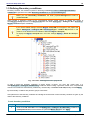
Flow V ision
Version 3.09.04
User's guide
© CAPVIDIA, 1999-2015 Leuven, Belgium. All rights reserved.
FlowVision Help
1
Contents
1 Quick start
2
1.1 Example of a problem
(mixing a liquid)
.......................................................................................................................3
1.2 Loading a geometric.......................................................................................................................4
model of a mixer
1.3 Operations in the View
window
.......................................................................................................................7
1.4 Defining general settings
of the project
.......................................................................................................................10
1.5 Defining Substances
and their parameters
.......................................................................................................................12
1.6 Defining Phases and
their parameters
.......................................................................................................................15
1.7 Defining a Model and
its parameters
.......................................................................................................................17
1.8 Indicating a Model .......................................................................................................................18
in calculation subregion
1.9 Defining Boundary.......................................................................................................................19
conditions
1.10 Defining Initial conditions
.......................................................................................................................24
1.11 Defining a computational
grid
.......................................................................................................................25
1.12 Defining simulation
controls
.......................................................................................................................30
1.13 Displaying results.......................................................................................................................33
1.13.1 Creating charachteristics
........................................................................................................................ 36
1.13.2 Creating layers........................................................................................................................ 38
1.14 Carrying out the project
calculations
.......................................................................................................................42
1.15 Monitoring the project
calculation process
.......................................................................................................................43
1.16 Creating an animation
.......................................................................................................................46
© CAPVIDIA, 1999-2015 Leuven, Belgium. All rights reserved.
FlowVision Help. Quick start.
2
1 Quick start
This section shows a case study of a full cycle of the project - from the formation of the project to analyze the
results.
After stepping through the actions described here, you will gain basic skills of working with the interface
FlowVision.
As an example, consider task fluid mixing in a mixer.
Sequence of actions:
1. Download the geometry
2. Discover basic operations in the View
3. Specify the general settings of the project
4. Ask Substances (In this example - one substance Water)
5. Ask Phase (Liquid water), and its parameters
6. Ask Model and its parameters
7. Specify Model in computational subregion
8. Ask Boundary conditions tap
9. Explore the concept Initial conditions
10.Ask a computational grid (ie, set Starting grid and configure Adaptation)
11.Set the control parameters calculation
1. Adjust the display of the results:
a. establishment characteristics
b. creation of layers
12.Practice with the procedures start, stop and continue the calculation
13.Adjust the control to calculate project
14.Create a series of graphic files Trending of the calculation time (Animation)
© CAPVIDIA, 1999-2015 Leuven, Belgium. All rights reserved.
FlowVision Help. Quick start.
3
1.1 Example of a problem (mixing a liquid)
Consider the flow of water in the mixer, which is a tank with two supply tube at the base and one outlet tube on the
cover:
Tank diameter is 0.04 m, the height of the cylindrical part of the tank - 0.02 m, height of the cover - 0.01 m,
diameter of the tubes - 0.01 m. Through one of the tubes served cold water (T = 0oC), through the other - hot (T =
70oC) the water flow in the supply tube is the same and equal to 0.1 kg -1.
The purpose of the calculation is to obtain the flow pattern and temperature equalization of water in a blender.
© CAPVIDIA, 1999-2015 Leuven, Belgium. All rights reserved.
FlowVision Help. Quick start.
4
1.2 Loading a geometric model of a mixer
The geometry of the computational domain, on the basis of which the project is created, create a software
package isFlowVisionin geometric modeling systems.
Formation of the project begins by loading the geometric model of the computational domain. Perform the following
steps:
Step
1
Actions
StartPre-Postprocessor(Start Button Windows> Programs> FlowVision>Pre-Postprocessor).
Window of Pre-Postprocessor will open.
Before the launch ofpre-postprocessorto be launched License Manager. Start
ofLicense Managercan be tuned so it can occur automaticallyat system startup. If
necessary,License Managercan be started manually via theStartbuttonWindows
(Start>Programs> FlowVisionLM>License Manager),or run it executable
(FvLicense.exeWindows orFvLicensein Linux).
2
Select main menu Choose File>New. The standard window for selecting a file.
3
Select the fileMixer.wrl, located in the folder:
C: \ Program Files \ TESIS \ FlowVision HPC \ Tutorial \ Samples \
Geom
or C: \ Program Files (x86) \ TESIS \ FlowVision HPC \ Tutorial \
Samples \ Geom
4
Dialog box to specify the name and location of the project:
Specify the name of the project in it in thename of the new folder(and, if necessary, the
location in theLocationfield), then clickOK.
In the client part of the project will create a subdirectory of the project that contains the client files
of the project. In the Project Tree tab Preprocessor appear loaded elements of the project.
After you create a project in the treePreprocessorerror messages are displayed in the geometry,
marked with "!":
load geometry to another Tolerance
in the context menu Region clickFix self-intersection
Use to correct errors in the geometry of a specialized package (for example,
3DTransVisia)
Loading a previously created and saved projectFlowVisionvia File>Open, where in the dialog
box select the appropriate project.
If you can not download the file geometry, then:
checkwhether he FlowVision supported format, and its elements are the requirements
send thefileto thegeometry technical support FlowVision with a description of the
problems encountered.
© CAPVIDIA, 1999-2015 Leuven, Belgium. All rights reserved.
FlowVision Help. Quick start.
5
5
In the review (4)pre-postprocessorappears loaded geometric model of the computational domain.
Window pre-postprocessor
In the illustration, the numbers are the components of the windowspre-postprocessor:
the main menu (1)
toolbars (2)
Projectwindow(3)
WindowView(4)
Propertieswindow(5)
Protocolwindow(6)
Monitoringwindow(7)
status bar (8)
In
the
project
window(3)the
project
Preprocessor,Solver,Postprocessor,Viewport.
tree
is
displayed
in
four
tabs:
After creating the project and download the geometrical model of the computational domain, all
folders of the project tree empty folders except the geometric model of the computational domain
and its display parameters:
Preprocessortabgeometric model of the computational domain is displayed in the
folderRegion>Subregions >subregion # 0>Geometry, automatically generated when
loading the boundary conditions are located atRegion>Subregions >subregion #
0>Boundary conditions;
Postprocessortabdisplay options boundary conditions are placed in folders3D-scene>
Objects> Computational space > Solids > Subregions > SubRegion # 0> Boundary
conditions and 3D-scene > Layers > Solids > Subregions > SubRegion # 0>
Boundary conditions.
In addition to the geometric model of the computational domain in the project
tabPostprocessorautomatically creates aplane # 0in the folder3D-scene> Objects>
Computational space. The plane is displayed in theView(4) the vertical line of blue color. Plane #
0is oriented perpendicular to the X axis and passes through the center of the computational domain.
This plane is not part of the geometric model of the computational domain, so it remains invisible to
the current in the mixer of the liquid (ie it - completely transparent to the liquid and has no influence
on it). The plane is necessary in order to display it on the calculated distribution of the values
computed characteristics and perform other auxiliary operations.
© CAPVIDIA, 1999-2015 Leuven, Belgium. All rights reserved.
FlowVision Help. Quick start.
6
© CAPVIDIA, 1999-2015 Leuven, Belgium. All rights reserved.
FlowVision Help. Quick start.
7
1.3 Operations in the View window
Before you generate the project, consider loaded geometric model of the computational domain.
Additional objectplane # 0in the folder 3D-scene>Objects>Computational spaceallows to cut part of the
geometric model. Operations in theViewwindow performed using the toolbar buttons and mouse.
Image of a geometric model of the computational domain
To adjust the image:
Step
Actions
1
Click the button to turn off the effect of perspective and be sure to click
surface geometric model).
2
Click
3
Click
enough (to fill the
to display facets, making up the framework of the model surface. Press this button.
for mode conversion type.
To rotate an image:
Step
Actions
1
Click the button
2
Click , , , , ,
get the views of the mixer along the axes of the coordinate system
associated with the model of the computational domain - absolute coordinate system.
to display the internal and external surfaces of the object
The contour of the cross section of the mixer object plane # 0 is displayed in blue.
3
In order to rotate the image of the mixer in theView:
a)
move the mouse pointer in theViewwindow
b)
click the left mouse button and keep it pressed, move the mouse pointer
For a reference, use the icon of the coordinate system, showing the unit vectors of the
coordinate system (in its default configuration it is located in the lower left corner of theView.
4
Click
to hide the external surfaces of the object and turn the faucet in the desired manner
(repeat steps3,4).
To offset and scale the image:
Step
1
Actions
In order to zoom in the mixer windowView:
a) move the mouse pointer in theViewwindow
b) rotate the mouse wheel.
Image is increased or decreased relative to the center of the windowView.
2
In order to shift the image in the mixerView
a) move the mouse pointer in theViewwindow
b) click the right mouse button and keep it pressed, move the mouse pointer.
3
To return to the original state of the image in theViewwindowand display the entire geometric
model of the computational domain, click .
© CAPVIDIA, 1999-2015 Leuven, Belgium. All rights reserved.
FlowVision Help. Quick start.
8
To display groups of facets that make up the geometric model:
The geometric model of the computational domain consists of several groups of facets (to display borders
groups, click ).
Step
Actions
1
Press
2
To display one of the groups of facets:
to activate the selection.
a) move the mouse pointer on the geometric model and click the left mouse button;
on the screen will be only one of the groups of facets lying beneath the point of clicks.
One side of the group is a front surface and painted (by holding down the ). On the
reverse side of the surface pattern applied to the group of fragments
;
b) after re-clicking the left mouse button on the screen will display the next group of
facets, which lies under the point-click (if available).
3
To display the entire geometric model, set the mouse pointer in theViewwindow is a geometric
model and click the left mouse button.
Cross-section of a geometric model of the plane
In order to cut off a plane geometric model of the computational domain:
Step
1
Actions
Perform the following two conditions:
plane should be cutting, which Postprocessor tab right-click the
scene>Objects>Plane # 0and set the mark in the paragraphto the View;
line3D-
geometric model of the computational domain must be cut-off, whichPostprocessor
tab right-click the line3D-scene> Objects> Computational space> Solids and
check the box in paragraph Apply clipping.
2
Highlight tab Postprocessor line 3D-scene>Objects>Plane # 0.
In the Viewwindow visible plane, the reference point on it, and coming from the reference point
of the vector normal to the plane. It can be seen that the plane cuts the negative half-space (the
normal vector in the positive half-watching).
To change the position of the plane with the mouse:
Step
Actions
1
Press
2
Highlight tabPostprocessorline3D-scene>Objects>Plane # 0.
3
To rotate the plane around the reference point, click the left mouse button and keep it pressed,
move the mouse pointer.
4
To move the reference point along the plane right-click and hold, and drag the mouse.
5
To move the reference point along the normal to the plane, press the left and right mouse button
and hold it, move the mouse pointer.
to select Edit object.
© CAPVIDIA, 1999-2015 Leuven, Belgium. All rights reserved.
FlowVision Help. Quick start.
9
Changing the position of the plane with the help of the window "Properties":
Step
Actions
1
Highlight tabPostprocessorline3D-scene>Objects>Plane # 0.
2
In thePropertieswindow, follow these steps:
for the orientation of the plane along the axis X (Y, Z), clickObject> Operations>
,
(
), And then clickApply;
to change the orientation of the plane on the opposite, clickObject> Operations>
and then clickApply.
© CAPVIDIA, 1999-2015 Leuven, Belgium. All rights reserved.
FlowVision Help. Quick start.
10
1.4 Defining general settings of the project
Some of the common parameters include values such as:
reference temperatureTref andpressurePref (default is 0oC and 101000 Pa)
vectorof gravitational accelerationin the absolute coordinate system associated with the geometric model
of the computational domain (gravityvector).In the example in the figure given the acceleration of gravity
9.8 m / s2in the directionagainst theaxis Y.
g-point- the coordinates (in the absolute coordinate system) the point at which a hydrostatic pressure
component vanishes
g-density -densityof a heavy fluid,situated above the g-point (as if the layers of a heavy fluid is not
specified, then the lower g-point), whichcontributes to the hydrostatic component of the pressure
Some of the general guidelines of the project also includes the definition of the layers of a heavy fluid, below the gpoints, each of which is characterized by the following parameters:
g-thickness- the thickness of a heavy fluid
g- density-densityof a heavy fluid in a given layer (lower layer and if the next layer is not defined)
The General settings are specified in the Properties of the element Region > General settings in the project
tree (in the tab Preprocessor):
Element "General settings" in the project tree
© CAPVIDIA, 1999-2015 Leuven, Belgium. All rights reserved.
FlowVision Help. Quick start.
11
Example of a common project settings
© CAPVIDIA, 1999-2015 Leuven, Belgium. All rights reserved.
FlowVision Help. Quick start.
12
1.5 Defining Substances and their parameters
Substanceis determined by the state of aggregation and properties.
Substancesare createdin the foldertreePreprocessor Substances. Aggregative state of aSubstanceis defined in
theSubstance's Propertieswindow. EachSubstancehas a set of child elements corresponding to physical
properties of the substance. Values of thesephysical propertiesofthe substance are defined in
thePropertieswindowsofappropriate child elements. Parameters of aSubstance in the projectcan be defined
manually or loaded fromtheSubstance Database. The number of substances may be one or more.
We define the physical properties of the current environment, which in this project is a single-phase and consisting
of one substance - water, considered as an incompressible fluid.
Setting substance
Step
1
Actions
Right-click the folder rowSubstancesPreprocessortab and chooseCreate.
In the folderSubstancesfolder is displayed new elementSubstance # 0.
2
Right-click the folder rowSubstance # 0,and then clickLoad from SD > Standard.
Downloaddialog box is displayedfrom the database:
3
SelectWaterin the drop-down listand the value ofLiquidSubstancesin the drop-down list
Phases, then clickOK.
In the folderSubstancesshows the new elementWater_Liquid.
4
Expand elementWater_Liquid.
Displays a list of physical properties of matter:
5
To view the specified properties (for example,viscosity):
a) scroll to theviscosity ofthe list of the physical properties of the substance; in
thePropertieswindowdisplays theviscosityparameter:
© CAPVIDIA, 1999-2015 Leuven, Belgium. All rights reserved.
FlowVision Help. Quick start.
13
b) In thePropertieswindow, click on theValuefield(on the field itself for data entry),
and then on the icon
. Tabledialog box is displayedf (x)with a tabulated
function of the viscosity of the pressure (X) and temperature (Y):
c) close thetable.
6
Specify a value of zero Enthalpy of formation(this option is only used in the model of
mass transfer with chemical reactions or burning)
a) highlight enthalpy of formation of the list of physical properties of the
substance
b) In the Properties window, click the mouse pointer on the row value and then
click on
:
c) drop-down list, select Constant
© CAPVIDIA, 1999-2015 Leuven, Belgium. All rights reserved.
FlowVision Help. Quick start.
14
d) in the input box set the value to 0, and then click Apply:
For reference: physical properties of water
Physical property
The value of
The dimension of
Density
1000
[Kg / m3]
Viscosity
0.001
Thermal conductivity
Specific heat
[Kg / (m
0.6
[W / (m K)]
4217
[J / (kg K)]
© CAPVIDIA, 1999-2015 Leuven, Belgium. All rights reserved.
FlowVision Help. Quick start.
15
1.6 Defining Phases and their parameters
Phase- a set of agents and the simulated physical processes.
Phases are defined in thePreprocessortreeinfolder Phases. The project should be at least one phase. Number of
phases is not limited.
We indicate what substance is phase and define the physical processes in the phase of which will be considered in
the calculation.
Setting phases:
Step
1
Actions
Right-click the folder Phases and select the Create continuous.
In yourfolder is displayed Phases new elementPhase # 0.
2
Expand the created element, right-click the lineand select thefolderSubstancesin itAdd / remove.
Dialog box, clickthe substance:
3
Select the desired substance in the list on the leftunselected(in our case -Voda_Zhidkaya) and
clickAdd.
The selected material is displayed in the right listselected.
4
ClickOK:
In the folderis displayedSubstancesadded element.
5
Select the item,Physical processesin the folderSubstances.
In thePropertieswindowdisplays a list of physical processes.
© CAPVIDIA, 1999-2015 Leuven, Belgium. All rights reserved.
FlowVision Help. Quick start.
6
16
Select the drop-down lists the physical processes in the following order:
parameter Heat transfer select from the list of value Convection & conduction
parameterMovement Motionselect from the list the value ofNewtonian fluid
Turbulenceparameter value, select from the list ofKES(standard k-ε turbulence model).
Please note thatwhile themovementMotion= (none) (None)turbulence model can not be
set)
7
ClickApply.
Specified items phase displayedin the project tree:
© CAPVIDIA, 1999-2015 Leuven, Belgium. All rights reserved.
FlowVision Help. Quick start.
17
1.7 Defining a Model and its parameters
Model- a set of phases and phase interactions.
Models are createdin the foldertreePreprocessormodels. The project should be at least one model. Number
of models is not limited.
In the presence ofseveralphasesin themodelscan be specifiedinterfacial interaction.
At this stage, the formation of the project will determine which phase is included in the model, and define the initial
data, which later will be given the initial conditions for the model equations.
Setting Model
Step
1
Actions
Open the context menu of the foldermodelsand select theCreatecommand.
In the folderModelsfolder is displayed new elementModel # 0.
2
ExpandModel # 0,right-click the lineand select thefolderPhasesitAdd / remove.
Dialog box, clickthe phase.
3
Select the desired phase in the left listUndrawn(in our case -Phase # 0),and then clickAdd.
The selected phase is displayed in the right listselected.ClickOK.
4
In the folderis displayedPhasesadded element. Initial folder. data> Setup. data # 0displays a
list of itemsInitial value of variable:
5
If you highlightin the project treeelementInitial value of variable,then in
thePropertieswindowdisplays the value of the initial data, which by default is zero. This
means that initially the liquid in the tank is at rest and at a temperature equal to the reference
value, i.e., 0 degrees Celsius.
For in this example (mixer)
Ask aModel:
In the context menu,selectCreate afolderModels
InPhasesin theModelsfolder# 0# 0addPhase
o In the context menu of a folderModel # 0>Phases, clickAdd / Remove
o In the form, select otryvsheysyaPhase # 0,and then clickAdd
© CAPVIDIA, 1999-2015 Leuven, Belgium. All rights reserved.
FlowVision Help. Quick start.
18
1.8 Indicating a Model in calculation subregion
We indicate the model estimated subregions (ie, subregions, which will be calculated), not doing it for the off-design
subregions.
To specify the model in the computational subregion:
Step
Actions
1
Select the folder in the project tree Subregions > Subregion #0.
2
In its Properties window, set the parameters of the Model by selecting from the
drop-down list, select Model #0:
3
Click Apply.
© CAPVIDIA, 1999-2015 Leuven, Belgium. All rights reserved.
FlowVision Help. Quick start.
19
1.9 Defining Boundary conditions
Boundary condition- the condition imposed on the design variableson borders of aSubregion.Boundary
conditionsare specified in the folder Boundary conditions in an appropriateSubregion.
Before you set theboundary conditionsin the folder propertiessubregionmust select a
predefinedmodel.
When loading a geometric model of the computational domain model surface is divided into groups of
facetsRegion- Group #N,listed on thePreprocessortabin the folder Subregions > Subregion #0 > Geometry >
Region- Surface # 0 (see. illustration).
If you use the default settings elements Region- Group #N do not appear in the project tree
(folders Subregions > subregion #N> Geometry>Region - Surface #N),because in real
problems it can lead to tens or hundreds of elements Region- Group #N).
To display the Region- Group #N set in the basic settings Display > Show All Groups =
Yes.
Fig. 3.2. Folder «Subregions»in the project tree
In order to place the boundary conditions on these groups of facets, you must first create them in a
folderSubregions > subregion # 0>Boundary conditions. When loading a geometric model of the computational
domain in this folder are automatically created only one boundary conditionB. Cond # 0(thermally insulatedWall).
By the boundary conditions are placed in groups more facets.
After placement of the boundary conditions and finding the surface area of each boundary condition are given by the
value of the boundary conditions.
Create boundary conditions
Step
1
Actions
Scroll to itemB. Cond # 0in the folderSubregions > subregion # 0>Boundary conditions,in
thePropertieswindow,set the valuefor the parameterWall's nameand click Apply.
© CAPVIDIA, 1999-2015 Leuven, Belgium. All rights reserved.
FlowVision Help. Quick start.
2
20
Open the context menu of a folderSubregions > subregion # 0>Boundary conditionsand
select theCreatecommand.
In the folder is added to itemB. Cond # 1.
3
Scroll to itemB. Cond # 1and in thePropertieswindow:
selectInlet / OutletType setting
specify a valuefor the parameterCold inletName
click Apply:
4
Make two copies of the boundary conditionLogin cold,opening the context menu on the
elementLogin coldand selecting theCopy.
In the folder are added elements includecold # 0and# 1 Login cold.
5
Select the itemLogin cold # 0in thePropertieswindow:
specify a valuefor the parameterincludes a hotname
ClickApply
6
Select the itemLogin cold # 1in thePropertieswindow:
Freeselectoutputtypesetting
set theoutputvaluefor the parametername
ClickApply
The alignment of the boundary conditions on the groups of facets
The alignment of the boundary conditions on the groups of facets produced enumeration groups and indicating
for each of them the desired boundary condition. Because all groups of facets is already a boundary
conditionWall, remains only to change the boundary conditions at the inlet and outlet sections of the
tubes.
Step
Actions
© CAPVIDIA, 1999-2015 Leuven, Belgium. All rights reserved.
FlowVision Help. Quick start.
21
1
If the itemsin the folderSubregions > subregion # 0>Geometry>Region- Surface #
0>Region- Group #Ndo not appear in the project tree, adjust their display in basic settings
FlowVision (Open the menu command File> Preferences,setting the Display > Show All
Groups = Yes).
2
Select the itemSubregions > subregion # 0>Geometry>Region- Surface # 0>RegionGroup #1, and in thePropertieswindow, selectOutputparameterboundary condition,and then
click Apply.
3
Select the itemSubregions > subregion # 0>Geometry>Region- Surface # 0>RegionGroup #6, and in thePropertieswindow, selectLogin coldparameterboundary condition,and
then click Apply.
4
Select the itemSubregions > subregion # 0>Geometry>Region- Surface # 0>RegionGroup #8, and in thePropertieswindow, selectLog hotboundary conditionfor the
parameter,and then click Apply.
Specifying the values of the boundary conditions
Step
Actions
1
In the folderSubregions > subregion # 0>Boundary conditions,highlight theLog cold,in
thePropertieswindow,find the sectional area of the supply tube - 7,7777591212273E-05 m2.
2
In the folderSubregions > subregion # 0>Boundary conditions>Login cold:
a) scroll to
theVelocity,
in
thePropertieswindow,set
the
valuefor
the
parameter1285.7mass velocity,and then click Apply; 1285.7 value obtained by
dividing the flow rate of 0.1 kg s-1by the area of the supply tube
7,7777591212273E-05 m2;
b) scroll to thetemperature, In thePropertieswindow, specify a value of 0 for the
parametervalue, and then click Apply.
3
In the folderSubregions > subregion # 0>Boundary conditions>Sign hot:
a) scroll to Velocity,in thePropertieswindow, set the valuefor the parameter1285.7mass
velocity,and then click Apply;
b) scroll to the temperature, in the Properties window,set the value of 70 for the
parameter value, and then click Apply.
© CAPVIDIA, 1999-2015 Leuven, Belgium. All rights reserved.
FlowVision Help. Quick start.
22
For in this example (mixer)
Ask four boundary conditions: Wall, Entrance for hot water, cold water entrance and Gate:
DefineModel # 0inSubRegion # 0
Boundary conditionsin the folderthrough the context menu, create three boundary conditions (one
already created by default)
Arrange the boundary conditions as indicated below:
Set the parametersof the boundary conditions:
o Boundary 1
Type
=Wall
Variables
Velocity
Temperature
TurbEnergy
TurbDissipation
= Logarithm law
= Zero flow
= Value in cell near wall
= Value in cell near wall
o Boundary 2
Type
=Inlet / Outlet
Variables
Velocity
Value
Normal = mass velocity
=1285.7
[Kg m -2s-1]
= Value
= 70
[C]
Temperature
Value
TurbEnergy
Value
TurbDissipation
Value
= Pulsations
=0
= Scale of turbulence
=0
[m]
o Boundary 3
Type
=Inlet / Outlet
Variables
Velocity
Value
Normal = mass velocity
=1285.7
[Kg m -2s-1]
= Value
=0
[C]
Temperature
Value
TurbEnergy
Value
TurbDissipation
Value
= Pulsations
=0
= Scale of turbulence
=0
[m]
o Boundary 4
Type
= Blank output
Variables
Velocity
Value
= Pressure
=0
Temperature
= Zero gradient
TurbEnergy
= Zero gradient
TurbDissipation
= Zero gradient
[Pa]
© CAPVIDIA, 1999-2015 Leuven, Belgium. All rights reserved.
FlowVision Help. Quick start.
23
© CAPVIDIA, 1999-2015 Leuven, Belgium. All rights reserved.
FlowVision Help. Quick start.
24
1.10 Defining Initial conditions
Initial conditions- this field values calculated variables in a given object initial time.
By default, all variables (except forthe phase volume)at the initial time are zero. Variablevolume phasehas a
default at the initial time value of1.
Set the initial conditions only if you want to start calculating with the values that differ from those used by default
(zero for all variables, except forthe phase volume,and a value of1for the variablevolume phase).
Initial conditions are defined in aSubregion.
Prior to theinitial conditionsin the folder propertiessubregion #imust select a predefinedmodel.
In order to set theInitial conditions
Set theModel Initial data:
1)
o Createinitial data
o Assign values to create an initialdata
Set theProperty:
2)
o Create anobjectfor the application ofthe initial conditionsin the folderObjects
o Set the parameters of the object
Set theInitial conditions:
3)
o Create afolder in theInitial conditionsInitial conditions in aSubregion
o Set the parameters ofInitial conditions
For in this example (mixer)
The initial conditions is not required.
Notes:
1)
Someinitial dataare always created in the default model.
2)
Computational spaceobjectis always created in the folderObjectsby default.
3)
SomeInitial conditions,containing theinitial data # 0and toComputational space are always automatically
createdin aSubregion.
Assignment of non-zero initial conditions is useful in order to accelerate the convergence of the solution (for
example, in the problems of external flow is convenient to define the initial velocity field corresponding to the free
stream velocity).
© CAPVIDIA, 1999-2015 Leuven, Belgium. All rights reserved.
FlowVision Help. Quick start.
25
1.11 Defining a computational grid
Computational grid- a set of cells into which the computational domain. The values of variables within a single cell
constant.
Specifyingthe computational gridincludes
Entering thestarting grid
SpecifyingAdaptation
Specifying the computational grid consists of two stages:
a) specify the start grid. In this example, set the initial uniform computational grid, ie with constant steps of
each of the coordinates with a number of steps:
NX= 20, NY= 20, NZ= 30;
b) job adaptation and adaptation to solution. In this example, set adaptation (local refinement) of the
computational grid near the boundaries of the region; adaptation to the solution not to ask.
Defining an initial grid
The initial grid is defined in dialog windowProperties of the initial mesh.
In order to setuniform Starting grid:
In thePropertieswindow, specify the numberof initial gridcells in each direction in the respective nX
nY nZ
In order to setan uneven Starting grid:
In the Properties window of the Initial grid element, call one of the Initial grid editors clicking on
or
In the window that appears, the corresponding Initial grid editor set grid options.
The flow in the mixer:
Ask a uniform initial mesh 20h20h30.
In the Properties window, set the initial grid:
nX = 20
nY = 20
nZ = 30
Perform the following steps:
© CAPVIDIA, 1999-2015 Leuven, Belgium. All rights reserved.
FlowVision Help. Quick start.
Step
1
26
Actions
On the Advanced tab,scroll to the folderPreprocessorInitial grid.
Inthe Viewwindowshows the computational domain in the "box":
2
In thePropertieswindow,set the number of steps for each coordinate: value <20> for the nX
and nY, the value of <30> for nZ, then clickApply:
Inthe Viewwindowshows the picture constructed initial computational grid:
© CAPVIDIA, 1999-2015 Leuven, Belgium. All rights reserved.
FlowVision Help. Quick start.
27
Specifying adaptation near the borders of the area
Adaptation- a partition of grid cells in each direction in half the specified number of times.
Level of adaptation- the number of consecutive partitions mesh.
Adaptationcan be defined on theboundary conditions,or at thefacility.
To be adaptedto theboundary conditions,follow these steps:
S
t
e
p
Actions
1 In thePropertieswindow Boundary conditionsincludingadaptationand set its parameters. For this
tabPreprocessorproject tree select the folderSubregions > subregion # 0>Boundary
conditions>Walland itsPropertieswindow, set the options:
a) setAdaptation> Enable = Yes(select from the list)
b) setAdaptation> Max. Level = 1
c) setAdaptation Layers> cells = 2
© CAPVIDIA, 1999-2015 Leuven, Belgium. All rights reserved.
FlowVision Help. Quick start.
28
2 Press Apply
The task of adaptation at the Facility
To specifyan Adaptationto theobject, follow these steps:
Step
Actions
1
Set theobjectin the folderObjects
2
Createan Adaptation #N folder Adaptation correspondingSubregion
3
Set the parametersAdaptations
© CAPVIDIA, 1999-2015 Leuven, Belgium. All rights reserved.
FlowVision Help. Quick start.
29
For in this example (mixer)
Set adaptation level 1 near the surface on which the identified boundary conditionWall:
In the properties of the boundary conditionsset Wall:
Adaptation
Yes
Level
1
Cell Layers
2
© CAPVIDIA, 1999-2015 Leuven, Belgium. All rights reserved.
FlowVision Help. Quick start.
30
1.12 Defining simulation controls
Setting calculation is carried out on thetab Solver.
The main control parameters calculation includes the step of integration of the model equations in time and stop
conditions calculation.
Specifying the time step
The time step is set in thePropertieswindow Time step.
The time step can be set:
permanent
by the Courant-Friedrichs number-Levy
In order to set the time step, in thePropertieswindowof the time step:
specify the way in which will be determined by the time step
then set the values needed to determine the time step chosen method
Constant step is recommended to set equal to 1/10 of the characteristic time. In the problem of
flow in the pipe as a typical time span can be selected - that it would take a particle released
from the entrance of the computational domain in order to reach the exit of the computational
domain. And the problem of flow around an aircraft as a characteristic linear dimension can
take the size of the device in the direction of flow, and as a characteristic velocity - the speed of
the incoming flow at infinity.
The flow in the mixer:
Ask apermanent step = 0.001s.
Setting conservation
The results of the calculation can be saved automatically in the process of calculating the specified interval. If
necessary, it is possible to preserve the history of calculation. You can store the data and layers. Saving data is
configured in the Autosave data. Saving layers can be adjusted in the AutoSave layers.
The operations with saved results inPre-Postprocessor:
Operation
Data
Layers
Running on the computation of a stored step
Yes
No
Visualization in touch withColverom
Yes
No
Visualization without regard toColverom
No
Yes
Beds of the parameters did not change after saving
Yes
Yes
Changed settings affecting the constructionCloya
Yes
No1)
Changed settings affecting the displayCloya
Yes
Yes
Visualization of layers created after calculating
Yes
No
Automatic sequential loading results in touch withColverom
Yes
No
Data
Layers
Yes
No
Visualization of layers created prior to the calculation of
The operations with saved resultsinViewer:
Operation
Visualization in touch withColverom
© CAPVIDIA, 1999-2015 Leuven, Belgium. All rights reserved.
FlowVision Help. Quick start.
31
Visualization without regard toColverom
Visualization of layers created after calculating
Automatic sequential loading results without regard to the solver
No
Yes
Yes
No
No
Yes
The flow in the mixer:
AskData autosavewith parameters:
History
Yes
Frequency
Type
By the time
The number of seconds
0.005
Notes:
1)
Visualization is performed using the build settings defined before saving.
Specifying Conditions stop
The calculation can be stopped manually by the user through buttons
accordance with the terms of the stop.
in the toolbar or automatically in
Break conditions:
1. The length of time - Payment stops at the specified time.
2. Iteration - Payment stops when the specified number of iterations
3. Residuals - Payment stops when all the created residuals calculated variables are below the specified
values
4. Custom values - Payment stops when all the residuals by custom variables are below the specified level.
Plot residuals calculated variables and values of user variables is displayed in theMonitortabPlot.
The flow in the mixer:
Set thelength of time:
Starting
0
Stop
1
Note:
Specifying Conditions shutdown is not necessary for the calculation.
Setting the control calculation for this example
Step
1
Actions
Solvertab, scroll to thetime step,and in thePropertieswindow, set the options:
a)
b)
Selectavaluein secondsfor theprocessparameters
set the value of0.01for theconstantparameterstep
© CAPVIDIA, 1999-2015 Leuven, Belgium. All rights reserved.
FlowVision Help. Quick start.
32
2
ClickApply.
3
On the Advanced tab,scroll to theSolverBreak conditions> The length of timeand in
thePropertieswindow,set the value ofparameter1Stop:
4
ClickApply.
© CAPVIDIA, 1999-2015 Leuven, Belgium. All rights reserved.
FlowVision Help. Quick start.
33
1.13 Displaying results
Displaying calculation results (visualization) is provided inPostprocessorusing Characteristics and Layers. The
conditions under which the mapping may depend on the manner in which the preservation of the results was
carried out (in the form of data or in the form of layers).
If carried storing data to display the results obtained, it is necessary:
open a project inPre-Postprocessor
connect toSolver
if necessary, to synchronize the client and server parts.
After that, thePre-Postprocessorwill display the last saved data. If necessary, you can create additional elements
Postprocessor.
If the data is saved to the history, you can view intermediate results (through the toolbar Navigation) and creating
animations (By the toolbar Pictures) with the mapping of the dynamics solutions in time.
Elements to display the results should be chosen depending on the type of the display data:
Data Type
Name of the element
Integral values:
Variable value on the surface and in the bulk
Characteristics
Local values:
Local values of the scalar variable along the line
Layer «Plot along line»
Layer «Plot along curve»
Layer «Plot along ellipse»
Local values of the scalar variable at the surface
Layer «Color contours»
Local values of the scalar variable in the amount of
Isosurface
VOF (Only for variable VoF, see section Theory>
Physical Processes> Transfer phase)
Local value and direction vector variable on the
surface and in the bulk
Layer «Vectors»
Layer «Streamlines» and element «Emitter»
Displaying various values:
The value of
Object
Feature / Layer
Variable in
the Properties
window
Variable in the
Data window
Integral values:
The flow through the
input or output
SupergroupCreate Characteristicsin the
d on the surface of corresponding
the input or output
Supergroup
Any list
Mass flow +
Mass flowVolumetric Flow
+
Volumetric flow-
The average speed in Plane section
the section
Characteristicson the
correspondingplanes
Velocity
<f surf.>
Average temperature
section
Plane section
Characteristicson the
correspondingplanes
Temperature
<f surf.>
The average
temperature of the
flow through the
section
Plane section
Characteristicson the
correspondingplanes
Temperature
<f mass+>
The average surface
temperature
SupergroupCreate Characteristicsin the
d on a given surface corresponding
<f mass->
Temperature
<f surf.>
© CAPVIDIA, 1999-2015 Leuven, Belgium. All rights reserved.
FlowVision Help. Quick start.
34
Supergroup
Force or moment
acting on a
streamlined body
SupergroupCreate Characteristicsin the
d on the surface of corresponding
the body
Supergroup
Any list
- F liq. X, Y, Z1)
- M liq. X, Y, Z1,2)
Position of the
Imported object,
Characteristicson the
center Moving body On which a Moving correspondingimport
body is created
objects
Any list
The center of
rotation X, Y, Z
Velocity of
movement Moving
body
Imported object,
Characteristicson the
On which a Moving correspondingimport
body is created
objects
Any list
Velocity X, Y, Z
Plot of the pressure
distribution along the
contour of the cross
section
Plane section
Pressure
The pressure
distribution in the
cross section
Plane section
Color contours
corresponding to Plane
Pressure
No
The velocity
distribution in the
cross section
Plane section
Vectors corresponding
to Plane
Velocity
No
The pressure
distribution on the
body surface
SupergroupCreate Color contours
d on the surface of corresponding to
the body
Supergroup
Pressure
No
Streamlines
Computational
space
Streamlines in Space
Velocity
No
Surface phase (only
in problems with the
contact surfaces)
Computational
space
VOF
No
No
Pressure in a given
volume (sensor)
Object
Characteristics to
facilities
Pressure
<f об.>
Local values:
Plot along curve
corresponding to Plane
3)
(Box or Ellipsoid /
sphere or Cone /
cylinder)
corresponding
sensor
4)
Create a layer and change its settings can be performed at any time
When conducting long-term calculations should always display the data in the calculation process, as in this
case, the user is able to permanent control over the process of convergence of the solution and, if necessary, to
intervene in the process of calculating when a numerical instabilities or divergence of solutions. Sometimes the
user makes a mistake when setting the option and the majority of these errors are detected in the first iteration of
the computational algorithm by observing the behavior of the solution.
Notes:
1)
Fliq. and Mliq., respectively, the force and the moment that the body acts on the flow. Force and the moment that
the flow acts on the body, are equal in magnitude and opposite in sign Fliq. and Mliq.
2)
The moment is defined relative to the center,whose coordinates are given in the Characteristics.
3)
When you create a Plot along curve requires that the curve was in the first quarter (quadrant) of the coordinate
system graph.
© CAPVIDIA, 1999-2015 Leuven, Belgium. All rights reserved.
FlowVision Help. Quick start.
35
4)
OnStreamlinesalso necessary to set thesource. As a source can be anyobject.
© CAPVIDIA, 1999-2015 Leuven, Belgium. All rights reserved.
FlowVision Help. Quick start.
36
1.13.1 Creating charachteristics
To control the output flow regime a steady state will monitor the temperature at the exit of the mixer. To do this,
follow these steps:
Step
1
Actions
First you need to select a computation Characteristics - A set of integral values (including
secondary) obtained after integration of a variable on the surface or in the bulk of the object. Job
characteristics is reduced to the direction of the variable and the object on the surface or
volume which should be integration.
To do this, select the output section to set up an a Supergroup- element of the project tree
containing facets, which supplied the output boundary condition.
We use the fact that the component characteristics included in the calculation of the number of
stopping criteria is displayed in the form of a graph in the Monitor, and define stopping
condition calculation the criterion on the basis of characteristics of components to the average
value of the variable.
To create Characteristicson a Supergroup:
Step
1
Actions
Open the tabcontext menu itemPreprocessorSubregions> subregion # 0>Boundary
conditions>Exit, and then click Create supergroup>preprocessor.
In the project tree is added created supergroup (in our example - an element Supergroup on
"Outlet"in the folderObjects):
2
Open the context menu on the element Supergroup on "Outlet" and select Create
characteristics.
A dialog box Create new characteristics block:
3
ClickOK.
© CAPVIDIA, 1999-2015 Leuven, Belgium. All rights reserved.
FlowVision Help. Quick start.
37
In the project tree element is added Characteristics # 0 (Supergroup on "Outlet"):
4
Select the elementCharacteristics# 0,in thePropertieswindow, select the valuefor the
parameterHighCharacteristics> Variableand clickApply.
To set the stop condition for calculating the criterion on the basis of characteristics:
Step
1
Actions
Open the tab Solver context menu item Break conditions > Custom valuesand select the
commandCreate:
In the project tree is added created a stopping criterion (in our example - an element ofa
stopping criterion # 0in the folderBreak conditions> Custom value):
2
Select the itemstopping criterion # 0,in thePropertieswindow,do the following:
a) selectCharacteristics # 0for the parameterobject
b) select <fweight->*)for the parametervariable(thereby setting the calculation of
average cross section of the outlet temperature of the waterflowingthrough the outlet)
c) select a value of 0 for the parameterlevel(that is, computation will be interrupted,
unless the characteristic will be constant over time) And clickApply.
© CAPVIDIA, 1999-2015 Leuven, Belgium. All rights reserved.
FlowVision Help. Quick start.
38
*)
If you select <fweight +>,it would mean computation for the water flowingthrough the outlet
that would have led to a null result.
For in this example (mixer)
Create Characteristics for Supergroup, the corresponding boundary conditions outlet:
Create based on the boundary conditions outlet a Supergroup in Postprocessor
Create Characteristics for Supergroup
In the Properties window Characteristicsset
Characteristics
Variable
Variable
Temperature
In order to maintain the momentum of change of temperature in the file, before the start of the
calculation set:
Save to File
Mode
Automatic
1.13.2 Creating layers
For visual inspection of the calculation will follow the velocity vectors and temperature in the two sections of the
mixer. To do this, follow these steps:
Step
1
Actions
First you need to create two planes:
one of them - the vertical plane of symmetry of the mixer
second - the horizontal plane passing through the axis of lead pipes
2
Further, these planes define layers that define the mapping in a color temperature of the fill, and
the speed - in form of vectors. Each layer displays a certain way only one variable and only one
object. It is therefore necessary to create two layers on the same plane, and two - on the other.
In one layer couples the temperature field to be displayed in the other - the velocity vector.
In order to set thelayer,
Create apreprocessor orPostprocessor Objectand set its properties
Create alayerto the created object
To create planes:
Step
1
Actions
Open the tabcontext menu itemPostprocessorObjectsand select the commandCreate. A
dialog boxCreate new object:
© CAPVIDIA, 1999-2015 Leuven, Belgium. All rights reserved.
FlowVision Help. Quick start.
39
2
Select theObject typefieldvalueplane, and then clickOK. In the project tree is added to
create a plane -Plane # 1itemin the folderObjects, which coincides with the desired
vertical plane of symmetry of the mixer.
3
Open the context menu on the elementplane # 1inObjectsfolderand selectCopy. In the
project tree, the plane -planeelement# 2in the folderObjects.
4
Scroll to the elementplane # 2and in thePropertieswindow,do the following:
a) clickObject> Operations>
and clickApply; plane will be horizontal;
b) select0.005for the parameterobject> reference point> Y,and then clickApply;
horizontal plane passes through the axis of the underwater tubes.
To set the layers:
Step
Actions
1
Open the context menu itemObjects> Plane # 1in tabPostprocessorand select the
CreateLayer. Dialog box opens Create new layer:
2
SelectColor contoursfor the parametertype layerand clickOK.
3
Open the context menu itemObjects> Plane # 1and select the CreateLayer.
4
In the dialog box, select the valuefor the parametervectorstype layerand clickOK.
5
Repeat steps1-4for the elementObjects> Plane # 2. In the project tree displays created four
layers:
© CAPVIDIA, 1999-2015 Leuven, Belgium. All rights reserved.
FlowVision Help. Quick start.
6
40
Set the parameters of both layersColor contours,highlighting an item in the project tree, and
performing the following steps in thePropertieswindow:
a) selecttemperaturefor Variable>Variable
b) selectManualfor settingrange> Mode
c) set
the
values
Minimum,respectively
of70and0fortheparameterrange>
High
andRange>
and clickApply.
7
Set the parameters of both layersvectors, selecting an item in the project tree, and
performing the following steps in thePropertieswindow:
a) selectVelocityfor Variable>Variable
b) specify a value of21for the parametersGrid>GridSize 1and> 2 Size
c) selectManualScaling> Mode
and clickApply.
The layers are defined in the folder Layers inPostprocessoron the basis of pre-createdobject.
© CAPVIDIA, 1999-2015 Leuven, Belgium. All rights reserved.
FlowVision Help. Quick start.
41
For in this example (mixer)
The flow in the mixer:
Ask two layersColor contoursfor the variabletemperature- one on the plane crossing the inlets, and the
other - on the plane of symmetry of the mixer:
Create twoplanes;
In theProperties windowof the firstplane is given by:
o Obj ects> Reference point>X = 0
o Obj ects> Reference point> Y = 0.005
o Obj ects> Reference point> Z = 0
o Obj ects> Normal> X = 0
o Obj ects> Normal> Y = 1
o Obj ects> Normal> Z = 0
In theProperties window the secondplane is given by:
o Obj ects> Reference point>X = 0
o Obj ects> Reference point> Y = 0.02
o Obj ects> Reference point> Z = 0
o Obj ects> Normal> X = 1
o Obj ects> Normal> Y = 0
o Obj ects> Normal> Z = 0
Create Layers ofColor contourson bothplanes
In theProperties window,setofLayers:Variable> Variable = Temperature
In order to display thetemperaturein the same scale on both layers, specify:
o Range>Mode = Manual
o Range>Maximum = 70
o Range>= 0 Maximum
© CAPVIDIA, 1999-2015 Leuven, Belgium. All rights reserved.
FlowVision Help. Quick start.
42
1.14 Carrying out the project calculations
Details on the calculation of the project start, stop and continue the calculationsee in section Start, stop, and
continue the calculation of project.
The following describes the launch of the calculation of this example.
For in this example (mixer)
Run the proj ect on the computation of pre-postprocessor:
Log onSolver-Agent:
o Press
in the toolbar
o In the next window, enter the user name and password on theSolver-Agent
Proj ect to the solver
o Press
in the toolbar
o In the window that appears, set the parameters of theSolver
o RunSolver
o Highlight runningSolverand clickConnect
RunSolverin computation
o Press
in the toolbar
o In the window that appearsStarting solveremove all tags
If necessary, stop computation via buttons
Authorization for theSolverpossible
theSolverrunSolver-Agent.
in the toolbar
only
when
the
Solver-Agent.
Before
operating
© CAPVIDIA, 1999-2015 Leuven, Belgium. All rights reserved.
FlowVision Help. Quick start.
43
1.15 Monitoring the project calculation process
The main methods of control in the process of calculation of the project are as follows:
basic control parameter calculation (including graphics predetermined stop condition calculation) in the
Monitor
imaging layers constructed in the course of computation;
control characteristics in the information windowInfo.
Control of the main parameters of the calculation in the «Monitor»
Select the display mode of theMonitorwindowand follow in the course of the calculation:
a) Statusmodeto track changes of the following parameters:
number of iterations, which should not significantly increase (strong growth means instability
account)
Algebraic residuals that must be within a predetermined accuracy of calculation
functional residuals, which should eventually decrease to a low value corresponding to steady flow,
or oscillate with a limited amplitude
b) Plotmodeto track the changes of the control parameter over time (see. figure).
Displaying a dependency ofthe control parameter from time to time in the «Monitor»
Displacement or stretching of the scale of the axes graph:
Step
Actions
1
Move the mouse pointer to the line axis of the graph.
2
After changing the shape of the pointer, press the left mouse button and keep it pressed, move
the mouse pointer along the axis.
3
Release the left mouse button.
Visual inspection of the project calculation
1. Press (Turn on / off the external surface)in the toolbar Solids, to make transparent object boundaries,
which enclose the interior space. This allows you to see the layers on the intersecting surfaces
(see. Figure).
© CAPVIDIA, 1999-2015 Leuven, Belgium. All rights reserved.
FlowVision Help. Quick start.
a)
44
b)
Displaying a field of temperature and vectors of velocity on layers:
and - an intermediate time point b - final result
2. Press
(View transformation mode)in the toolbar Modes to select the conversion type and choose the
most convenient angle for the analysis of the flow.
Control characteristics in the information box «Info»
Highlight the project tree line characteristics, and then click
(See the information box)in the toolbar Modes.
Window opensInfo(Fig. 3.5) with the parameters characteristics(para 7.6.1),calculated on the last time step
(their values are updated at the end of the next time step).
© CAPVIDIA, 1999-2015 Leuven, Belgium. All rights reserved.
FlowVision Help. Quick start.
45
Fig. 3.5. Information window «Info»with parameters "Features # 0"
© CAPVIDIA, 1999-2015 Leuven, Belgium. All rights reserved.
FlowVision Help. Quick start.
46
1.16 Creating an animation
Animation is created from a set of graphic files created either during the account or when viewing saved data.
These image files contain the image of the window View.
Here is how to create animation in thePre-Postprocessorduring counting.
Note:Similar opportunities are also available in animation Viewer.
Creating animation during counting
Step
Actions
1
Set the layers, the image which you want to save. On the layers is recommended to
setRange = Manualto the range and, accordingly, the color of layers depending on the
displayed variable values did not change from step to step.
2
Press
(Start Capture sequence Begin sequence)in the toolbar Pictures.Dialog box
opensImage Capture:
3
Ask in theImage Capturesettings (size, elimination of aliasing). ClickOK.
(For a detailed description of the elements of this window, see. Section Management of
capturing images).
4
This opens the standard Windows operating system to access the files (SaveImage).
Specify the location, type, and name prefix for the files that will be written to the image.
Then click theSavebutton.
Images will be written to the file at each updatewindowView.
The file names are formed as follows:
(Prefix) _00000. (Filetype)
(Prefix) _00001. (Filetype)
(Prefix) _00002. (Filetype)
etc.
5
Create a video from a sequence of image files saved with the help of a specialized
program.
The flow in the mixer:
Create animation in the process of changing the account of thetemperaturedistributionin the planes
described in the example in section Creating layers.
© CAPVIDIA, 1999-2015 Leuven, Belgium. All rights reserved.