Download COMCOT User Manual for version 1.6

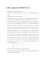
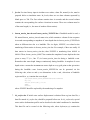
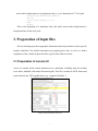
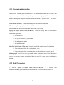
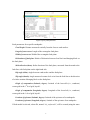
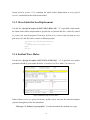
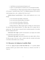
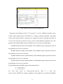
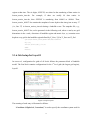
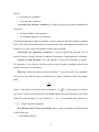
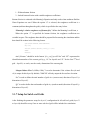
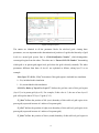
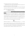
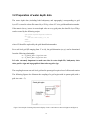
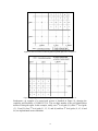
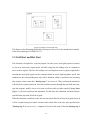
COMCOT User Manual
Version 1.6
(Drafted on Sep 19 2006)
(Updated on Feb 26 2007)
School of Civil and Environmental Engineering, Cornell University
Ithaca, NY 14853, USA
1
Journey of COMCOT
COMCOT, COrnell Multigrid COupled Tsunami model, originated from the work of S.N. Seo
based on Shuto’s model (Aug.10, 1993) and Yongsik Cho arranged version 1.0 (Aug.10, 1993).
A significant improvement was achieved by Seung-Buhm Woo (1999, 3). Many features,
including nonlinear model, Automatic Initial surface interpolation, general grid matching and
user interface, were introduced and finally formed version 1.4. However, at this stage, the code
was still not well organized and there were limitations in many aspects (e.g., grid setup, initial
condition ...), especially efficiency, capability and flexibility. The code, at that time, was
written in Fortran 77 and inconveniently, needed to be recompiled for each new simulation.
Many achievements were made on COMCOT during this period, such as the successful
simulations of 1960 Chile Tsunami and 1986 Taiwan Hua-lien tsunami, involving the
calculations of runup and inundation.
The coming of Fortran 90 gave a new power to the programming of this code. With the helps
of many others, especially Tom Logan (ARSC), Steven Lantz (Cornell) and Philip L.-F. Liu
(Cornell), further improvements and modifications were introduced by Xiaoming Wang (2003),
which yielded version 1.5. The most significant progress is the migration from Fortran 77 to
Fortran 90, allowing dynamic allocation of memory. Parameter module was introduced,
making the code much neat and readable. And subroutines dealing with nonlinear equations
were also optimized to get a better efficiency by Tom Logan (ARSC, 2003). Furthermore,
many redundant or unnecessary subroutines were either removed or combined together,
including subroutines pqstill, pqtotal, mass, mass_s, mass_c, moment, momt_s, momt_c,
ini_mvd, jnzoa, jnqoa, et_o_prt, et_a_prt, et_b_prt, etc. Some subroutines were renovated or
completely rewritten, including subroutines involving parameter input and data output. Old
parameter setup files, comcot_common.inc and comcot_v_1_4.inc, were removed and their
data entries were incorporated into comcot_v_1_4.ctl. In addition, new features were added in
version 1.5, like Cartesian coordinate support for the 1st level grid (layer 1), submarine
landslide model, Okada’s fault model, given static initial surface profile, given time history
data input in incident wave maker (used for benchmark problem 2 in Catalina Workshop 2003).
Unlike its previous versions which only allow one-to-one grid hierarchy (each grid can contain
only one sub-level grid), in version 1.5, 1st level grid (layer 1) can employ up to 4 2nd level
grids (layer 2s) although sub-level grids still use one-to-one grid hierarchy. This gives more
flexibility for a simulation if multiple sub-regions are of interest. The code was compacted
from about 5,000 lines to roughly 3,700 lines with enhanced capability, efficiency and
flexibility. However, the development of version 1.5 was an on-going process. With new bugs
identified and new features added in, the code was modified frequently on different
requirements, yielding several variations of version 1.5. Numerical simulations performed on
this version include 2002 Hua-lien tsunami, 2003 Algerian tsunami, 2004 and 2005 Indian
2
Ocean tsunamis and 2006 Java tsunami. For the 2004 Giant Tsunami, both runup and
inundation were extensively studied in several regions.
Gradually, more and more pressure was brought in the rollout of a new version, which should
be more stable, efficient, user-friendly and most of all, comprise all the features developed
before. Finally, version 1.6 comes. In this version, a brand-new user interface is designed
which requires only one parameter file, comcot.ctl, containing all the parameter setups for
incident waves, fault models, landslide model and grid information. The grid hierarchy is no
longer one-to-one. In each grid level, up to 4 sub-level grids can be implemented
simultaneously (Figure 10). Hot start function is also added to allow a simulation being
resumed from a specified time step. Although lots of tests are made to make sure results
consistent with its previous, bugs and errors may still exist. Please send your feedback to
[email protected].
More details for version 1.6 are illustrated in the following sections in this document.
Xiaoming Wang
Sep 20, 2006
3
1. Introduction
COMCOT adopts staggered leap-frog finite difference schemes to solve Shallow Water
Equations. A nested grid system, dynamically coupled up to four regions (which will be
referred to as layers) with different grid resolution, is adopted in the model to fulfill the need
for tsunami simulations in different scales. Nested grid system means in a region of one grid
size, there is one or more regions with smaller grid sizes situated in, which eventually, forms a
hierarchy of grids, or grid levels. The region with largest grid size is called 1st level grid and
all the grid regions directly nested in the 1st level grid, are called 2nd level grids, so on and so
forth. In one grid region, up to 4 sub-level grid regions can be defined. It should be noted that
in one grid region, a uniform grid size is adopted in COMCOT. Spherical or Cartesian
coordinate system, as well as either linear or nonlinear version of governing equations can be
chosen for each region. The initial free surface deformation due to a submarine earthquake is
assumed the same as the vertical displacement of the sea floor as long as the uplift motion is
much faster than the wave propagation; otherwise, submarine landslide model should be used
to include transient motion effect. For a given earthquake, the displacement of seafloor is
determined from a linear elastic dislocation theory (Manshinha and Smylie, 1971, or Okada,
1980). For theoretical background and detailed derivations, please refer to Liu, P. L.-F., Woo,
S.-B. and Cho, Y.-S. (1998) "Computer programs for tsunami propagation and inundation",
Cornell University.
4
2. Files required in COMCOT v1.6
The following files are included in this package.
1. comcot.exe: The executable program of COMCOT v1.6 (in Windows platform, x86,
32-bit).
2. comcot.f90: The source code (in Fortran 90).
3. comcot.ctl: Parameter file for COMCOT v1.6, including information for fault model,
incident wave maker, landslide model and all the grids implemented in a simulation.
4. layerXY.dep: Input water depth files containing both bathymetry data and topography data
for each grid (or layer) implemented in a simulation. “XY” represents the Identification
Number (ID) of a grid. “X” denotes the level of a grid in the hierarchy of a nested grid
system and “Y” stands for the numbering of this grid in its grid level. For example, layer23
means that it is a 2nd level grid (X=2) and it is the 3rd one (Y=3) in its level. In version 1.6,
the grid with the largest grid size is the 1st level grid, called layer01, and in one simulation,
up to 4 regions of sub-level grids can be implemented in layer01, which are layer21,
layer22, layer23 and layer24. Generally, in one grid region, regardless of its level, up to 4
sub-level grid regions can be nested in. Water depth file for each grid is generated by the
following code, where nx and ny are the x and y dimensions of the grid region and array
h(nx,ny) contains the water depth data. In a grid region, the origin of the coordinate system
is situated at the lower left corner with x axis pointing upward (northward) and y axis
pointing rightward (eastward).
open (25,file='layerXY.dep',status='unknown')
do i=1, ny
write (25, '(10f9.3)') (h(i, j), i=1, nx)
enddo
close(25)
where XY should be replaced by the grid identification number.
If, in a simulation, time history input in incident wave maker or landslide model is used,
additional data files will be required.
5
5. fse.dat: For time history input in incident wave maker, a data file, named fse.dat, must be
prepared before a simulation starts. In fse.dat, there are two data columns separated by
blank space or Tab. The first column contains time in seconds and the second column
contains the corresponding free surface elevations in meters. These two columns must be
of the same length (i.e., the same of number of data entries).
6. bottom_motion_time.dat and bottom_motion_XXXXXX.dat: if landslide model is used, a
file named bottom_motion_time.dat must exist, which contains a column of time sequence
in seconds corresponding to snapshots of water depth data in bottom_motion_XXXXXX.dat
taken at different time due to a landslide. The six digits, XXXXXX, are related to the
numbering of data entries in bottom_motion_time.dat. For example, if there are totally 44
data entries in bottom_motion_time.dat, then XXXXXX is numbering from 000001 to
000044. Then, bottom_motion_000027.dat contains the snapshot of water depth at the time
given at entry 27 (i.e., line 27) in bottom_motion_time.dat during a landslide event.
Remember that water depth changes continuously during landslide. A snapshot of water
depth at time t means the instantaneous water depth at every grid point at that given time
during the landslide event. bottom_motion_XXXXXX.dat can be generated via the
following code, where nx and ny are dimensions in the x and y directions of landslide
region and h(nx, ny) contains the water depth
open (25,file='bottom_motion_XXXXXX.dat',status='unknown')
do j=1, ny
write (25, '(F10.5)') (h(i, j), i=1, nx)
enddo
close(25)
where XXXXXX should be replaced by the numbering of a snapshot.
7. ini_surface.dat: If initial water surface displacement is obtained from a given data file, a
data file named ini_surface.dat, should be prepared before run. In ini_surface.dat, special
water surface deformation profile can be described as the initial condition of a simulation.
This data file can be created via the following code, where deform(nx,ny) contains the
6
water surface displacement at each grid point and nx, ny are dimensions of 1st level grid.
open (25,file=’ini_surface.dat’, status='unknown')
do j=1, ny
write (25, '(15f8.3)') (deform(i, j), i=1, nx)
enddo
close(25)
Then, at the beginning of a simulation starts, this initial water surface displacement is
interpolated into all sub-level grids.
3. Preparation of Input files
The user should prepare the topographic information and focal parameters for the specific
tsunami simulation. The detailed information on preparing these files, as well as a further
explanation of the variable in input data files is given in the follows sections.
3.1 Preparation of comcot.ctl
comcot.ctl contains all the control parameters for a simulation, including setup for incident
wave maker, landslide, fault model and nested grids. This file is written in ASCII format and
can be edited in any TXT-capable editor (e.g., wordpad, UltraEdit ...).
Figure 1 First 36 lines in comcot.ctl
7
3.1.1 Generation information
The first block contains general information for a simulation, including total run time, data
output interval, type of initial surface profile generation, starting type (cold start or hot start)
and the resuming time step. For each line, parameter should be specified after ‘:’ in “Value”
field.
“Total run time (seconds)” defines the total physical duration to be simulated.
“Time interval for output file ( unit: sec )” defines the time interval (in seconds) to output
data (including free surface elevation, and volume flux if specified).
“Specify ini surface (0:FLT,1:File,2:WM,3:LS)” is used to specify how the initial surface
deformation is generated:
0 – by fault model
1 – by a given data file, ini_surface.dat
2 – by incident wave maker
3 – by landslide model
“Start Type (0-Cold start; 1-Hot start)” is used to specify the starting type of a simulation.
0 – Start a simulation from the very beginning, t=0s;
1 – Start a simulation from a resuming time step where data are previously saved.
“Starting step #” specified the time step number where a simulation starts from if hot start is
used or, the time step number when related data are saved for a later restart if cold start is
selected.
3.1.2 Fault Parameters
If in the line “Specify ini surface (0:FLT,1:File,2:WM,3:LS)”, “0” is selected, fault
parameters should be given under the block “Parameters for Fault Model” in comcot.ctl.
8
Figure 2 specify fault parameters
Fault parameters for a specific earthquake:
Focal Depth: Distance measured vertically from the focus to earth surface.
Length of source area: Length of the rectangular fault plane.
Width of source area: Width of the rectangular fault plane.
Dislocation of fault plate: Relative Dislocation between foot block and hanging block on
the fault plane.
Strike direction (theta): Strike direction of the fault plane, measured from the north to the
fault line, with fault plane on the right-hand side.
Dip angle (delta): Angle between earth surface and the fault plane.
Slip angle (lamda): Angle measured counter clock wise from the fault line to the direction
of relative motion of hanging block on the fault plane.
Origin of computation (Latitude, degree): Latitude of the lower-left (i.e., southeast)
corner grid in the 1st level grid, layer01.
Origin of computation (Longitude, degree): Longitude of the lower-left (i.e., southeast)
corner grid in the 1st level grid, layer01.
Location of epicenter (Latitude, degree): Latitude of the epicenter of an earthquake.
Location of epicenter (Longitude, degree): Latitude of the epicenter of an earthquake.
If fault model is selected, a data file, named “ini_surface.dat”, will be created (using the same
9
format given in section 3.1.3), containing the initial surface displacement at every grid of
layer01, calculated from the built-in fault model.
3.1.3 Given Initial Surface Displacement
If in the line “Specify ini surface (0:FLT,1:File,2:WM,3:LS)”, “1” is specified, which means
the initial water surface displacement is specified in an external data file, a data file, named
ini_surface.dat, must be prepared. If an array, deform (nx,ny), stores water elevation at every
grid in layer01, this file can be created via following scripts
open (25,file='ini_surface.dat',status='unknown')
do j=1,ny
write (25,'(15f8.3)') (deform(i,j),i=1,nx)
enddo
close (25)
3.1.4 Incident Wave Maker
If in the line “Specify ini surface (0:FLT,1:File,2:WM,3:LS)”, “2” is specified, wave maker
parameters should be given under the block “Parameters for Wave Maker” in comcot.ctl.
Figure 3 Parameter setup for wave maker
Either solitary waves or a given time history profile can be sent into the numerical domain
(layer01) through any of the four boundaries.
“Wave type ( 1: Solitary, 2:given profile )” is used to determine the incident wave type:
10
1 – Send Solitary wave into the numerical domain, layer01.
2 – Input a wave profile defined in a time history file, fse.dat, through one boundary.
3 – Focused solitary wave. When using this option, incident wave through a boundary
will converge to a specified location ("focus"). Two additional parameters will be asked for
when the program starts: x and y coordinates of the focus in layer01.
“Incident direction( 1:top,2:bt,3:lf,4:rt )” defines which boundary the wave is sent
through.
1: waves come from the top boundary of the domain;
2: waves come from the bottom boundary of the domain;
3: waves come from the left boundary of the domain;
4: waves come from the right boundary of the domain;
5: Oblique incident wave. When using this option, an oblique wave will be sent into
the numerical domain through boundaries. The oblique angle will be required after the
program starts. The angle ranges is measured from the northward (upward) to the incident
direction, ranging from 0 to 360.
“Characteristic Wave height” specifies the characteristic wave height of the incident
wave (only effective when solitary wave is sent in).
“Characteristic Water depth” specifies the characteristic water depth, which is effective
for both wave types. This value is used to calculate volume flux associated with incident
waves based on linear shallow water wave theory.
3.1.5 Parameters for Submarine Landslide Model
If in the line “Specify ini surface (0:FLT,1:File,2:WM,3:LS)”, “3” is specified, landslide
parameters should be given under the block “Parameters for Submarine Land Slide” in
comcot.ctl.
11
Figure 4 Parameter setup for submarine landslide model
Compared to the dimension of the 1st level grid (i.e., layer01), landslide, generally, occurs
within a small confined region. In COMCOT v1.6, during a submarine landslide, water depth
in that small confined region is required to be sampled at locations coincident with grids of
layer01 at the time given in bottom_motion_time.dat, which should be prepared by user. The
position of the small landslide region is defined in layer01 in terms of its grid indices.
“X_Start” defines the left (west) boundary of the landslide region expressed in terms of
the grid index of layer01 in x direction.
“X_End” defines the right (east) boundary of the landslide region expressed in terms of
the grid index of layer01 in x direction.
“Y_Start” defines the lower (south) boundary of the landslide region expressed in terms of
the grid index of layer01 in y direction.
“Y_End” defines the upper (north) boundary of the landslide region expressed in terms of
the grid index of layer01 in y direction.
The grid dimension of landslide region can be obtained from
nx = X_End-X_Start+1
ny = Y_End-Y_Start+1
For
each
time
given
in
bottom_motion_time.dat,
there
is
a
data
file,
bottom_motion_XXXXXX.dat, storing a snapshot of water depth at every grid in the landslide
12
region at that time. The six digits, XXXXXX, are related to the numbering of data entries in
bottom_motion_time.dat.
For
example,
if
there
are
totally
44
data
entries
in
bottom_motion_time.dat, then XXXXXX is numbering from 000001 to 000044. Then,
bottom_motion_000027.dat contains the snapshot of water depth at the time given at entry 27
(i.e., line 27) in bottom_motion_time.dat during a landslide event. The snapshot file, e.g.,
bottom_motion_000027.dat, can be generated via the following code, where nx and ny are grid
dimensions in the x and y directions of landslide region and matrix h(nx, ny) contains water
depth at every grid in the landslide region defined by X_Start, X_End, Y_Start and Y_End.
open (25,file='bottom_motion_000027.dat',status='unknown')
do j=1, ny
write (25, '(F10.5)') (h(i, j), i=1, nx)
enddo
close(25)
3.1.6 Grid setup for Layer01
In comcot.ctl, configuration for grids of all levels follows the parameter block of landslide
model. The first block contains configurations for the 1st level grid (the largest grid region),
layer01.
Figure 5 Setup for layer01
The meaning of each entry is illustrated as follows.
“Coordinate (0:Spherical, 1:cartesian)” is used to specify the coordinate system used for
13
layer01.
0 – Use Spherical coordinates
1 – Use Cartesian Coordinates
“Governing Eqn. (0:linear, 1:nonlinear)” is used to specify the governing equations used
for layer01.
0 – Use linear shallow water equations.
1 – Use nonlinear shallow water equations.
It should be noted that if spherical coordinate system is adopted, only linear shallow equations
can be used. Moving boundary scheme (associated with runup and inundation calculation) in
COMCOT v1.6 only works with nonlinear shallow water equations.
“Grid length (dx, sph:minute, cart:meter)” is used to specify the grid size (Δx) of
layer01 in meters if using Cartesian Coordinates or in minutes if using Spherical Coordinates.
“Latitude of south boundary” gives the latitude of south (lower) boundary of layer01.
This parameter is not effective if all the grids are using Cartesian coordinates and the fault
model is not chosen in a simulation.
“Time step” defines the time step (Δt) used for the 1st level grid, layer01, in a simulation.
The grid size (Δx) and time step (Δt) should satisfy Courant Condition to make the program
stable
CΔt
< cr ,
Δx
where C is the phase speed which can be evaluated as C = gh . g is the gravity acceleration
(g=9.81m/s2) and h is the characteristic water depth (should choose the maximum water depth
which will yield the largest C). For COMCOT, cr < 0.5 is recommended (may allow up to
cr < 0.7 if linear equation is adopted).
“Use Bottom friction ?(only cart,nonlin,0:y,1:n)” is used to determine if bottom friction
is used in this grid.
0 – With bottom friction
14
1 – Without bottom friction.
2 – Include bottom friction with variable roughness coefficients
Bottom friction is evaluated with Manning’s Equation and only works when nonlinear Shallow
Water Equations are used. When the option “0” is selected, the roughness coefficient is a
constant (uniform throughout the grids), which is specified at the entry below.
“Manning's relative roughness coef.(bottom fric)” defines the Manning’s coefficient, n.
When the option “2” is specified for bottom friction, the roughness coefficients are
variable in space. The roughness data should be prepared before starting the simulation and the
data should be written in the following format:
open (25,file=filename, status='unknown')
do j=1, ny
write (25, '(10f9.5)') (lo%fric_vcoef (i, j), i=1, nx)
enddo
close(25)
And “filename” should be in the format “fric_coef_layerXX.dat” and “XX” represents the
identification number of the current grid (e.g., ‘01’ for layer01 and “21” for the first 2nd-level
grid – layer21). nx and ny are the x and y dimension of the current grids
“Output Volume Flux ? ( 0-Yes, 1-No )” is used to determine if the volume flux (uh and
vh) is output for this layer. By default, COMCOT will only output the free surface elevation.
“ix” is used to define the total number of grids in x (west-to-east) direction of layer01 (x
dimension of layer01).
“jy” is used to define the total number of grids in y (south-to-north) direction of layer01 (y
dimension of layer01).
3.1.7 Setup for Sub-Level Grids
After finishing the parameter setup for layer01, configuration for all sub-level grids (layer21
to layer44) should be set up if one or more sub-level grid will be included in a simulation.
15
Figure 6 Setup for layer21
The entries are identical in all the parameter blocks for sub-level grids. Among these
parameters, two are important to the determination of position of a grid in the hierarchy of grid
levels in a nested grid system. One is “Grid Identification Number”, which distinguishes
current grid region from the others. The other one is “Parent Grid’s ID Number” determining
which grid is its parent grid (upper-level grid where the grid is directly situated). The other
parameters different from those of layer01 are explained as follows, taking layer21 as an
example.
“Run Layer 21? (0:Yes, 1:No)” determines if this grid region is included in a simulation.
0 – Yes, included in this simulation
1 – No, not included in this simulation
“Grid Size Ratio of Layer01 to Layer21” defines the grid size ratio of this grid region
(layer21) to its parent grid (layer01). For example, if this value is 5, the area of one layer01
grid will equal to that of 25 layer21 grids (5×5).
“X_Start” defines the position of left (west) boundary of this sub-level grid region in its
parent grid (expressed in terms of x indices of its parent grid).
“X_End” defines the position of right (east) boundary of this sub-level grid region in its
parent grid (expressed in terms of x indices of its parent grid).
“Y_Start” defines the position of lower (south) boundary of this sub-level grid region in
16
its parent grid (expressed in terms of y indices of its parent grid).
“Y_End” defines the position of upper (north) boundary of this sub-level grid region in its
parent grid (expressed in terms of y indices of its parent grid).
Therefore, this rectangular sub-level grid region is outlined by its four corners in its parent grid:
(x_start,y_start), (x_end,y_start), (x_end, y_end) and (x_start, y_end). The total number of
grids in x and y directions can be calculated as
nx = (X_End-X_Start+1)*grid size ratio
ny = (Y_End-Y_Start+1)*grid size ratio
It should be mentioned that the 2-digit grid identification number must be kept untouched
by users. The first digit indicates the level of this grid region in the hierarchy of nested grid
system (ranging from 2 to 4). The second digit, ranging from 1 to 4, stands for the numbing of
the grid region in its grid level. The grid level is defined in terms of the largest grid region (the
1st level grid, named layer01). Grid regions, directly nested in the 1st level grids (layer01), are
called 2nd level grids. And grid regions, directly nested in a 2nd level grids (e.g., layer21), are
called 3rd level grids, so on and so forth. Up to 4 grid levels can be defined in COMCOT v1.6.
In each sub-level grid, to make the program stable, the Courant Condition,
CΔt
< cr ,
Δx
should also be satisfied, and cr < 0.5 is recommended (may allow up to cr < 0.7 if linear
equation is adopted). By default, the time step of a sub-level grid is half of that of its parent
grid. Grid size of a sub-level grid is determined by that of its parent grid and the grid size ratio.
If, for a sub-level grid, the grid size of its parent grid is 10.0m and the grid size ratio of this
sub-level grid to its parent is 5, the grid size of this sub-level grid is 10.0/5=2.0m.
17
3.2 Preparation of water depth data
The water depth data (including both bathymetry and topography) corresponding to grid
layerXY is stored in a data file named layerXY.dep, where XY is its grid identification number.
If the matrix h(nx,ny) stores its water depth value at every grid point, the data file layerXY.dep
can be created by the following scripts
open (25,file='layerXY.dep',status='unknown')
do i=1, ny
write (25, '(10f9.3)') (h(i, j), i=1, nx)
enddo
close(25)
where XY should be replaced by the grid identification number.
For a sub-level grid (ID ranging from 21 to 44), the grid dimension (nx,ny) can be determined
from the following relationship
nx = (X_End-X_Start+1)*grid size ratio
ny = (Y_End-Y_Start+1)*grid size ratio
It is also extremely important to make sure that in water depth file, bathymetry data
takes positive sign and topographical data takes negative sign.
The coupling between one sub-level grid and its parent grid requires lots of efforts and caution.
The following figures also illustrate the coupling of a grid region with its parent grid (with a
grid size ratio = 3).
Figure 7 An example of nested grid (zoom-in display of zone 1 and zone2 are shown in figure 8 and figure 9)
18
Figure 8 Lower-left corner of sub-level grid in its parent grid (zone 1 in figure 7)
Figure 9 Upper-right corner of sub-level grid in its parent grid (zone 2 in figure 7)
Furthermore, an example of a nested grid system is sketched in Figure 10, showing the
capability and flexibility of COMCOT v1.6. The two-digit number is the grid identification
number of that grid region. In this example, totally, one 1st level-grid (01), three 2nd level grids
(21, 23 and 24), four 3rd level grids (31, 32, 33, and 34) and four 4th level grids (41, 42, 43 and
44) are implemented in one simulation.
19
Figure 10 Example of nested grid setup
This figure is also illustrating the default grid setup in comcot.ctl for the attached test example
in the release package of COMCOT v1.6.
3.3 Cold Start and Hot Start
This function is designed for a special purpose. In some cases, small grid regions of interest
are far away from source region and it will take a long time for leading wave of a tsunami to
arrive at these regions. The time for leading wave traveling from source region to right before
entering the small grid regions can be estimated based on water depth and phase speed, and
furthermore, the corresponding time step will be obtained, which is specified as the resuming
time step for a later restart after "Starting step # " in comcot.ctl. Then, cold start the simulation
with all sub-level grids turned off. After the simulation passes through that specified time step,
stop the program, modify comcot.ctl to turn on all the sub-level grids required, change Start
Type to 1 (Hot Start) and rerun the simulation. For this time, the simulation will start from the
specified time step with all sub-level grids.
When this function is enabled, for the first run, three data files for the first-level grids (layer01)
will be created storing free surface elevation and volume flux at the time step specified after
"Starting step #" in comcot.ctl (i.e., snapshot of layer01 at this step). If the time Starting step #
20
= 1000, the three data files will be z1_01_001000.dat, m1_01_001000.dat and
n1_01_001000.dat. In the next run (hot start), these files will be loaded in as the initial
condition for this restart.
COMCOT will also automatically save resuming snapshots of all grids every 1000 time
steps for later start. To resume from any of these saved snapshots, changing the “start_type”
option to 2 and specifying the starting time step after “starting step#”, the simulation will start
from the specified time step.
4 Output Data
Generally, only the free surface elevation will be output in data files named in the form
z_AB_dddddd.dat, where "z" stands for free surface elevation, two digits " AB" denote the
corresponding grid identification number and the six digits, "dddddd", corresponds to the time
step number when the data is output. Therefore, data file z_AB_dddddd.dat stores the free
surface elevation at all grid points in grid region layerAB at time step dddddd. For example,
z_23_001234.dat stores the free surface elevation at all grid points of layer23 at time step
1234. It should be mentioned that the total number of time steps required for a simulation and
also time step number for data output are also calculated based on the time step (Δt) of layer01.
For example, if 0.5s time step is used for layer01, the time step number 1234 corresponds to a
physical time t=1234*0.5=617.0s.
However, if the switch "Output Volume Flux" is set to "0" for layerAB, two additional types of
data files, m_AB_dddddd.dat and n_AB_dddddd.dat will be created, storing volume flux data
in x direction and y direction, respectively, at all the grid points in layerAB at time step
dddddd.
The following scripts will be able to read the data in a output data file "F_AB_dddddd.dat"
into a predefined matrix B(nx,ny)
open (25,file='F_XY_dddddd.dat',status='unknown')
do i=1, ny
read (25, '(15f9.3)') (B(i, j), i=1, nx)
21
enddo
close(25)
where F denotes "z", "m" or "n"; AB represents Identification Number of a grid region and
"dddddd" stands for the time step # at which the data is written.
In addition, if the switch "Output Volume Flux" is set to "2", neither water surface
elevation nor fluxes will be out.
22
5. Example
A set of sample data files is included in the package of COMCOT v1.6. The default
configuration in comcot.ctl defines a nested grid setup illustrated in Figure 10. The dimensions
for all grid regions are all the same, 100*100. The grid size and time step for layer01 are
10.0m and 0.025s, respectively. A constant water depth, 10.0m, is used and a solitary wave
with amplitude 0.5 m is sent into layer01 through its lower boundary. The other three
boundaries use open boundary condition. Two snapshots of layer01 at t=50s and t=100s are
shown in Figure 11.
Figure 11 Wave field Snapshots of layer01
23