1
WinDOAS 2.1 Software User Manual Caroline FAYT Michel VAN ROOZENDAEL February 2001 BIRA-IASB WinDOAS 2.1 Software User Manual February 2001 WinDOAS is distributed without any restrictions. In case of publications making use of WinDOAS, please mention the following authors in the acknowledgements. Michel VAN ROOZENDAEL Caroline FAYT [email protected] [email protected] Phone number Fax number 32 (2) 373.04.16 32 (2) 374.84.23 Mail address IASB/BIRA Avenue Circulaire, 3 B-1180 UCCLE BELGIUM Users may also contact the authors for spectra format adaptations, remarks, suggestions and technical support. Table of Contents 1 INTRODUCTION.................................................................................................................7 Purpose of the Document ..................................................................................................................................7 References .............................................................................................................................................................7 Overview of the Document ...............................................................................................................................8 INSTALLING WINDOAS ....................................................................................................9 2.1 System and Hardware Requirements................................................................................................................9 2.2 Installation .............................................................................................................................................................9 2.3 Associate wds File Extension with WinDOAS................................................................................................9 DESCRIPTION OF THE USER INTERFACE ...................................................................11 3.1 The User Interface Components.................................................................................................................... 11 3.2 The Four Main Windows in WinDOAS....................................................................................................... 12 The Environment Workspace Window........................................................................................................ 12 The Projects Window......................................................................................................................................... 12 The Data Window ............................................................................................................................................... 12 The Graphs Window .......................................................................................................................................... 12 3.3 The Main Menu Bar.......................................................................................................................................... 12 3.4 The Toolbar ....................................................................................................................................................... 13 3.5 The Status Bar.................................................................................................................................................... 14 3.6 The Shortcut Menus ......................................................................................................................................... 14 DESCRIPTION OF THE ALGORITHMS...........................................................................15 4.1 Main WinDOAS features ................................................................................................................................ 15 4.2 Block-diagram structure of the programme ................................................................................................. 16 4.3 Slant column fitting........................................................................................................................................... 21 The Beer-Lambert law ........................................................................................................................................... 21 DOAS fitting........................................................................................................................................................ 21 Intensity fitting....................................................................................................................................................... 22 4.4 Fit Parameters.................................................................................................................................................... 22 Absorption cross sections ........................................................................................................................................ 22 Polynomial............................................................................................................................................................. 24 Shift and Stretch.................................................................................................................................................... 24 Offset Correction .................................................................................................................................................... 24 Ring Effect............................................................................................................................................................. 25 Undersampling Correction...................................................................................................................................... 25 Standard Deviations of The Fitted Parameters ...................................................................................................... 25 AMF .................................................................................................................................................................... 26 Graphical Display Of Spectral Fit Results ............................................................................................................ 26 4.5 Wavelength calibration and slit function characterisation ......................................................................... 27 4.6 Off-line tools...................................................................................................................................................... 27 Convolution/Filtering Tool.................................................................................................................................... 27 Ring Tool .............................................................................................................................................................. 30 Undersampling Tool .............................................................................................................................................. 31 QUICKSTART...................................................................................................................33 5.1 Creating a Project.............................................................................................................................................. 33 Creating a New Project.......................................................................................................................................... 33 Inserting Files ........................................................................................................................................................ 34 Browsing Spectra.................................................................................................................................................... 34 Handling Graphs .................................................................................................................................................. 35 Saving Your Work................................................................................................................................................ 36 5.2 Example : Configuration of a Project for BrO Retrieval ........................................................................... 36 Configuring A Project For Spectra Analysis.......................................................................................................... 36 Description of sample.wds....................................................................................................................................... 37 Analysis Setup For BrO Retrieval......................................................................................................................... 38 Defining Symbols................................................................................................................................................... 38 Projects Properties .................................................................................................................................................. 38 Analysis Window Properties.................................................................................................................................. 42 Running Analysis.................................................................................................................................................. 44 1.1 1.2 1.3 2 3 4 5 6 THE WORKSPACE ENVIRONMENT TREE.....................................................................49 Creating a New Item in the Workspace Environment Tree ..................................................................... 49 Observation Sites Properties........................................................................................................................... 50 User-Defined Symbols Properties.................................................................................................................. 50 Handling Items in the WorkSpace Environment Tree .............................................................................. 50 7 THE PROJECTS TREE ....................................................................................................51 7.1 Description of the Projects Tree .................................................................................................................... 51 7.2 Directories and Files Management................................................................................................................. 52 Spectra Files .......................................................................................................................................................... 52 User-defined Folders .............................................................................................................................................. 52 Directories structures .............................................................................................................................................. 52 Handling Spectra................................................................................................................................................... 53 7.3 Handling Items In The Projects Tree .......................................................................................................... 53 7.4 Project Properties.............................................................................................................................................. 54 The Spectra Tab Page............................................................................................................................................ 55 The Analysis Tab Page ......................................................................................................................................... 56 The Filtering Tab Page.......................................................................................................................................... 57 The Calibration Tab Page ..................................................................................................................................... 58 The Undersampling Tab Page ............................................................................................................................... 60 The Instrumental Tab Page ................................................................................................................................... 61 The Slit Function Tab Page................................................................................................................................... 61 The ASCII Results Tab Page ............................................................................................................................... 62 The NASA-AMES Results Tab Page................................................................................................................ 64 7.5 Analysis Windows Properties.......................................................................................................................... 65 7.6 Configuration of the Fitting Parameters ....................................................................................................... 67 The Molecules Pages .............................................................................................................................................. 67 The Continuous Functions Page............................................................................................................................. 70 The Predefined Parameters Pages ........................................................................................................................... 71 The Shift and Stretch Pages ................................................................................................................................... 72 The Gaps Page ...................................................................................................................................................... 75 The Outputs Pages................................................................................................................................................. 75 7.7 Configuration of the Wavelength Calibration procedure .......................................................................... 76 The Molecules pages ............................................................................................................................................... 76 The Continuous Functions Page............................................................................................................................. 78 The Predefined Parameters Page............................................................................................................................. 78 The Shift and Stretch Pages ................................................................................................................................... 79 The Gaps Page ...................................................................................................................................................... 79 The Outputs Page.................................................................................................................................................. 79 8 THE WINDOAS TOOLS ...................................................................................................81 8.1 Supported line shapes....................................................................................................................................... 81 8.2 About Files Formats......................................................................................................................................... 81 8.3 The Convolution/Filtering Tool .................................................................................................................... 82 The General Tab Page........................................................................................................................................... 82 The Slit Function Tab Page................................................................................................................................... 83 The Filtering Tab Page.......................................................................................................................................... 84 8.4 The Ring Tool.................................................................................................................................................... 84 8.5 The Undersampling Tool................................................................................................................................. 86 9 ANNEXES.........................................................................................................................87 9.1 Files format ........................................................................................................................................................ 87 Calibration ............................................................................................................................................................ 87 Cross Sections ........................................................................................................................................................ 87 Solar Spectrum ...................................................................................................................................................... 87 Reference spectrum.................................................................................................................................................. 87 AMF .................................................................................................................................................................... 88 Slit functions.......................................................................................................................................................... 88 9.2 Troubleshooting ................................................................................................................................................ 89 6.1 6.2 6.3 6.4 Acronyms and abbreviations AMF ASCII BrO Cic DOAS ERS FT FWHM GOME IASB-BIRA MDI nm NDSC NLLS OHP RAM RMS RRS SCD SFP SVD SZA VCD Air Mass Factor American Standard Code for Information Interchange Bromine monoxide Colour Index Differential Optical Absorption Spectroscopy European Remote Sensing Satellite Fourier Transform Full Width at Half Maximum Global Ozone Monitoring Experiment Belgian Institute for Space Aeronomy Multiple Document Interface nanometers Network for the Detection of Stratospheric Change Non Linear Least Squares Observatoire de Haute Provence, France Random Access Memory Root Mean Square Rotational Raman Scattering Slant Column Densities Slit Function Parameter Singular Value Decomposition Solar Zenith Angle Vertical Column Densities This page is intentionnally left blankThis page is intentionnally left blank WinDOAS 2.1 February 2001 Introduction 1 Introduction 1.1 Purpose of the Document WinDOAS is a software developed at IASB/BIRA for analysis of UV-visible spectra by the method of Differential Optical Absorption Spectroscopy (DOAS) [12]. It takes the advantage of the experiment acquired by IASB/BIRA from early nineties in DOAS measurements and analysis. Several European groups of the DOAS community contribute also to the improvement and the evolution of the software by their helpful suggestions, applications and inter-comparison exercise. A separate version, GWinDOAS, has been developed for GOME, (Global Ozone Monitoring Experiment), a nadir-viewing UV-visible spectrometer aboard on the European satellite ERS-2. GOME measures the solar radiation back scattered from the atmosphere in the spectral range 230-800 nm with a high spectral resolution allowing the observation of minor trace gases implied in the ozone depletion, like BrO. 1.2 References [1] Aliwell, S. et al, Mid-latitude observations of the seasonal variation of BrO, 1. Zenith-sky measurements, Geophys. Res. Letter. 24, 1195-1198 (1997); [2] Bevington, P.R., Data reduction and error analysis for the physical sciences, Mc Graw-Hill Book Company (?) [3] Burrows, J.P. et al, Atmospheric remote-sensing reference data from GOME : Part 2. Temperature dependent absorption cross sections of O3 in the 231-794 nm range, JQSRT, 1998; [4] Chance, K., Analysis of BrO measurements from the Global Ozone Monitoring Experiment, Geophys. Res. Lett., 25, 3335-3338 (1998) [5] Chance, K. and Spurr R.J.D., Ring effect studies; Rayleigh scattering, including molecular parameters for rotational Raman scattering and the Fraunhofer spectrum, Applied Optics, 36, 5224-5230 (1997); [6] Hermans, C. et al., Absorption Cross-Sections of Atmospheric Constituents : NO2, O2 and H20, ESPR, 6 (3) 151-158 (1999); [7] Kaiser, J.F. and W.A. Reed, Data smoothing using low-pass digital filters, Rev. Sci. Instrum., Vol 48, 1447-1457 (1977); [8] Kuntz, M., a new implementation of the Humlicek algorithm for the calculation of the Voigt Profile Function, JQSRT, Vol.57, no 6, pp. 819-824, 1997. [9] Kurucz, R.L., I. Furenlid, J.Brault and L.Testerman, Solar flux atlas from 296 nm to 1300 nm, National Solar Observatory Atlas No. 1, 1984. [10] NDSC Database User's Manual (June 1999); [11] Press et al., Numerical Recipes in C, Cambridge University Press (1988-1991); [12] Platt, U. in Air Monitoring by Spectroscopic Techniques, Chap.2, ed. Markus W. Sigrist, Chemical Analysis Series, Vol. 127, p.27-84 (1994); [13] Vountas, M., V.V.Rozanov and J.P.Burrows, Ring effect : Impact of Rotational Raman Scattering on Radiative Transfer in Earth’s Atmosphere, Page 7 WinDOAS 2.1 February 2001 Introduction JQRST, Vol.57, no 6, pp. 819-824, 1997; [14] Wahner, A. et al., Absorption cross-section of BrO between 312 and 385 nm at 298 and 223 K, Chem. Phys. Lett., 152, 507-510 (1988); 1.3 Overview of the Document Chapter 2 : Installing WinDOAS This chapter covers system and hardware requirements and guide you in the installation of the software. Chapter 3 : Description of The User Interface This chapter covers the main components of the WinDOAS user interface : Chapter 4 : Description of The Algorithms This chapter summarises the main features of WinDOAS and describes the structure of the programme and the nature of the coded algorithms. Chapter 5 : Quickstart This chapter describes how to create a project, insert files and display spectra. Using a predefined configuration provided with the package (set up for BrO retrieval), it guides you step by step towards complete configuration of a project. Chapter 6 : The Workspace Environment Tree This chapter describes how to manipulate and configure Observation Sites and User-defined symbols items in the Workspace Environment tree. Chapter 7 : The Projects Tree This chapter describes the organisation, the handling and the configuration of the different kinds of items in the Projects tree. It covers : the four child windows; the menu bar; the toolbar; the status bar; the right-click shortcut menus. the management of files and directories structures in the Projects tree; the configuration of projects; the parameterisation of the analysis; the parameterisation of the wavelength calibration. Chapter 8 : The WinDOAS Tools This chapter covers the main features supported by WinDOAS about convolution and describes the three off-line tools included in the software : the Convolution/Filtering tool; the Ring tool for creating Ring effect cross sections; the Undersampling tool for creating undersampling cross sections. Chapter 9 : Annexes Page 8 Description of the format of input files and troubleshooting. WinDOAS 2.1 February 2001 Installing WinDOAS 2 Installing WinDOAS 2.1 System and Hardware Requirements WinDOAS runs under Windows 95/NT. A Pentium computer with at least 64 megabytes of RAM is recommended. 2.2 Installation The program with the “Software User Manual” (this document) and on-line help is usually distributed by E-mail. To install the package, just copy the sent files in a dedicated directory. The example application described in section 5.2 is available on request. 2.3 Associate wds File Extension with WinDOAS The configuration of applications developed with WinDOAS is saved in ASCII files. The default extension for WinDOAS configuration files is wds. You can open an existing configuration file using the options sequence Files-Open from the menu bar or the icon Open from the toolbar. The same result will be obtained easier by double clicking on the name of any file with extension wds. For that, apply the following instructions : • • • • • • • • • • • • in My Computer or Windows Explorer window, apply the command View-Options from the menu bar; select the File Types tab page; click New Type pushbutton; enter WinDOAS as Description of type; enter *.wds as Associated extension; click New pushbutton to open a New Action popup window; enter WinDOAS as Action; use Browse pushbutton to search for WinDOAS program in your path tree; click OK; click Change Icon pushbutton and then Browse pushbutton to search for WinDOAS program; select WinDOAS icon; Click ok. Page 9 This page is intentionnally left blank WinDOAS 2.1 February 2001 Description of The User Interface 3 Description of The User Interface 3.1 The User Interface Components Figure 3-1 : The WinDOAS User Interface Menu Bar Toolbar Projects Tree Workspace Environment Tree Data Window Right-click Shortcut Menu Graphs Window Status Bar The WinDOAS user interface is a Multiple Document Interface (MDI) including the following components : four main child windows; 1. the Workspace Environment window; 2. the Projects window; 3. the Data window; 4. the Graphs window. a menu bar; a toolbar; a status bar; right-click shortcut menus. These components are further detailed in the following sections. Page 11 WinDOAS 2.1 February 2001 Description of The User Interface 3.2 The Four Main Windows in WinDOAS The Environment In this window, the user should list all relevant symbols that will be used in the Workspace Window configuration of his projects and analysis windows. The Observation Sites coordinates are used to (re-)calculate zenith angles. For balloons and satellite measurements, they allow operating a selection on spectra to analyse, according to specified geolocation coordinates (the sites). The Projects WinDOAS is based on the notion of projects. A project can be defined as a set Window of files sharing the same configuration of analysis. WinDOAS allows defining several projects in a session, giving users the possibility to handle several analysis configurations. A project includes the definition of spectral windows and the list of files to analyse with this configuration. The Data Window This window displays the available information on the current spectrum and analysis results. The Graphs Window Spectra, fitting results and in general, any kind of graphical information, are displayed in the Graphs window. 3.3 The Main Menu Bar Application Control Files usual Windows options for applications control : New starts a new WinDOAS application; Open opens an existing WinDOAS application; Save saves the current WinDOAS application; Save as renames the current WinDOAS application; Print prints the content of the active Graphs or Data window; Print Setup selects and set up the printer; Exit exits WinDOAS Edit for the moment, this option only includes the Goto sub-option giving direct access to any record in the current open spectra file; Projects global operations on the Projects tree : New Remove All Run Analysis Run Calibration Tools Page 12 creates a new project in the Projects tree removes all projects from the Projects tree; applies analysis on all files of all projects; applies wavelength calibration on all files of all projects; gives access to WinDOAS tools; WinDOAS 2.1 February 2001 Description of The User Interface Windows Organization Online Help 3.4 View calls back the selected child window; Windows usual Windows options for organising child windows in the current application or activating the selected child window; Help gives access to online help. The Toolbar New Save Zoom out First spectrum Next spectrum Continue Stop Figure 3-2 : WinDOAS toolbar Open Print Goto Previous spectrum Last spectrum Pause The WinDOAS toolbar proposes several shortcuts that allow easy access to the following options : Application Control New starts a new WinDOAS application; Open opens an existing WinDOAS application; Save saves the current WinDOAS application; Printing Print prints the content of the active Graphs or Data window; Display Zoom out graph zoom in is performed by clicking and dragging the mouse over the wanted screen area; this shortcut recovers the original size of the active graph; Goto direct access to a given record in the current spectra file; First spectrum goes back to the first spectrum in the current file; Previous spectrum goes back to the previous spectrum in the current file; this button speeds up the spectra browsing when held down; Next spectrum goes to the next spectrum in the current file; this button also speeds up the spectra browsing when held down; Last spectrum goes to the last spectrum in the current file; Continue continues the paused spectra browsing or analysis; Pause in non-stop spectra browsing or analysis, marks a pause; Stop stops spectra browsing or analysis. Spectra Browsing Page 13 WinDOAS 2.1 February 2001 Description of The User Interface 3.5 The Status Bar The status bar is divided in three sections : 3.6 online help a short help text is displayed as a menu bar command or a shortcut menu option is pointed out with the cursor; graphs coordinates the current coordinates (in user units) are displayed as the cursor is moved on the graph; time section the current time is displayed with an accuracy of 1 minute. The Shortcut Menus Menu commands and toolbar buttons are completed in right-click shortcut menus. The options proposed in the shortcut menus depend on the calling object : the Data window, a graph or any item in the Workspace Environment or Projects trees. Page 14 WinDOAS 2.1 February 2001 Description of The Algorithms 4 Description of The Algorithms This chapter summarises the main features of WinDOAS and describes the structure of the programme and the nature of the coded algorithms. 4.1 Main WinDOAS features Analysis DOAS/intensity fitting modes; shift/stretch fully configurable for any spectral item (cross section or spectrum); possibility to filter spectra and cross sections before analysis (supported filters include Kaiser, gaussian, boxcar, Savitsky-Golay…); possibility to define gaps within fitting intervals (e.g. to eliminate bad pixels); possibility to fit an instrumental offset; possibility to work either in pixel or in wavelength (nm) units; possibility to define several configurations of spectral windows under a project; Calibration And Slit Function Characterization wavelength calibration and instrumental slit function characterisation using a non-linear least-squares (NLLS) fitting approach where measured intensities are fitted to a high resolution solar spectrum degraded to the resolution of the instrument. The fitting method (DOAS or intensity fitting) can be chosen different from the method used in the analysis; possibility to correct for atmospheric absorption and Ring effect; supports different analytical line shapes, as described in section 4.6; Cross Sections Handling possibility to calculate differential absorption orthogonalisation or high-pass filtering); cross sections (by possibility to correct cross sections using wavelength dependent AMF; possibility to fix the column density of any selected species; possibility to convolute cross sections in real-time using a user-defined slit function or the information on calibration and slit function provided by the wavelength calibration procedure; possibility to handle a difference of resolution between measured and control spectra; Undersampling possibility to build undersampling cross sections using the information derived from the NLLS wavelength calibration; Page 15 Description of The Algorithms Output Tools WinDOAS 2.1 February 2001 The output is fully configurable. Analysis results are saved in tabbed columns ASCII files, easily loadable in most spreadsheet programmes. Convolution/Filtering tool : standard and I0-corrected convolutions are supported; possibility to create an effective slit function taking into account the (finite) resolution of the source spectrum (using a FT deconvolution method); Ring tool : calculates Ring effect cross sections (Rotational Raman Scattering approach); Undersampling tool : generates undersampling cross sections; 4.2 Block-diagram structure of the programme The overall structure of the programme is schematically described in the following figures. Figure 1 describes the general organization of the processor. The structures of the wavelength calibration and slant column fitting modules are given in Figures 2 and 3, while the coupled linear/non-linear least squares fitting algorithm is sketched in Figure 4. Page 16 WinDOAS 2.1 February 2001 Description of The Algorithms I nitial wavelength calibration λ Control spectrum I0 (λ) Cross sections σ i Pre-processing Wavelength calibration (wc ) and slit function characterisation (SFP ) Apply NLLS fit to high resolution Frauhnofer reference spectrum (see Fig. 2) Apply wavelength calibration Convolute and/or interpolate σ i using wc and SFP Select fitting method (DOAS/Intensity fitting) Processing Spectra Load spectra Slant columns fitting Apply a NLLS fit to deduce slant columns densities of fitted absorbers (see Fig. 3) AMF Interpolation of AMF on the spectra SZA Convert Slant columns into Vertical columns ( VCD = SCD / AMF ) All fitted parameters SCD and VCD Standard deviations Figure 4-1. Overall structure of the spectral analysis programme. Page 17 WinDOAS 2.1 February 2001 Description of The Algorithms Initial wavelength calibration λ Control spectrum S High-resolution solar spectrum Cross sections σ i Select calibration interval and split into N sub-windows Select fitting method (DOAS/Intensity fitting) Slant columns fitting (see Fig. 3) Derive in each interval n : • • • The shift between solar n et S n ; Fitted slit function parameters SFP n ; SCD of correcting absorbers (e.g. Ring, O3 ) Determine the new wavelength calibration (wc) by polynomial fitting through the N individual shift values Determine wavelength dependency of fitted slit function parameters (SFP n (λ)) by polynomial fitting through the N individual SFP n values Display calibration results (optional) wc, SFP(λ ) Figure 4-2. Structure of the wavelength calibration module. Page 18 WinDOAS 2.1 February 2001 Description of The Algorithms I , I 0 , σ i , λ , NL Module performed at project pre-processing level if σ i matrix can be kept static Cross sections processing σ i correction with wavelength dependent AMF (optional) AMF ( λ,SZA) Convolute/Interpolate/Shift σ i Low-Pass filtering Generate differential σ i (by orthogonalisation or HP- filtering) Spectra processing Shift I (or I 0 ) Offset correction (applied on measured spectra) Decompose the fitting function into linear/non-linear parts (according to the selected fitting method) NLLS-FIT (see Fig. 4) Residual R Fitted parameters (included SCD) Standard deviations Figure 4-3. Structure of the slant column-fitting module. Page 19 WinDOAS 2.1 February 2001 Description of The Algorithms I , I 0 , σi , λ I, I 0 low-pass and high pass filtering (optional) Non linear parameters initialization NLLS fit Modify NL parameters according to the NLLS fit using a gradient-search algorithm combined with a linearization of the fitting function (Marquardt-Levenberg) Solve linear problem (LLS fit) Minimization of the residual R for linear parameters using SVD method 2 ∆χ < ε y Residual R fitted parameters (including SCD) standard deviations Figure 4-4. Structure of the coupled linear/non-linear least squares algorithm used in the slant column fitting module and in the wavelength calibration module. Page 20 WinDOAS 2.1 February 2001 4.3 Description of The Algorithms Slant column fitting The Beer-Lambert The Beer-Lambert law describes the extinction of the solar radiation in an law absorbing atmosphere : I(λ)=I0 (λ).exp( –Σ σi ci ) (eq. 1) where : I(λ) is the solar spectrum after absorption; I0 (λ) is the extraterrestrial solar spectrum; σi are the relevant cross sections of the absorbing species, with wavelength and temperature dependent structures; ci are the unknown species column densities. The logarithm of the ratio of the control spectrum (I0 (λ)) and the measured spectrum (I(λ)) is denoted optical density (or optical thickness): log(I0(λ)) – log(I(λ))=Σ σi ci (eq. 2) Two fitting analysis methods are implemented (DOAS and intensity fitting) in WinDOAS. They differ in the expression of the fitting function (use of the equation 1 or the equation 2. DOAS fitting The DOAS approach is a direct application of the equation 2. High frequency spectral structures of the various absorbing species are used to resolve the corresponding contributions to the total optical density. This is obtained using a least-square procedure where the slant column densities (SCD) of the various species are the fitted parameters. Large band contributions to the atmospheric attenuation (Rayleigh and Mie scattering) are accounted for by a low order polynomial function. Simply stated, the DOAS technique is a linear problem. This linearity is unfortunately broken down by the need to account for additional effects, namely: • small wavelength shifts between I and I0 spectra must be corrected using appropriate shift and stretch parameters; • possible instrumental and/or atmospheric straylight or residual dark current signal require the introduction of an offset parameter. In addition to shift and offset, Ring and undersampling effects have to be treated. See section 4.4 to have an overview of all parameters to fit. Let us consider the modified equation : Log(I(λ)–offset(λ))=log(I0 (λ)) –Σ σi ci –P+U (eq. 3) with P, the polynomial and U, the undersampling cross section (Ring effect cross section is simply included as an additional pseudo-absorber). In DOAS fitting mode, WinDOAS minimises residuals of equation 3 using a Marquardt-Levenberg non-linear least-squares (NLLS) algorithm. The method implements a gradient-expansion algorithm [2], which is based on the iterative combination of a steepest-descent method (suitable for approaching the minimum from far away) and a linearisation of the fitting function. Page 21 WinDOAS 2.1 February 2001 Description of The Algorithms Linear parameters are determined by a Singular Value Decomposition (SVD) method [11] embedded in the NLLS algorithm. Intensity fitting WinDOAS also supports the so-called intensity fitting (or direct fitting) method where measured intensities are directly fitted instead of their logarithms. This corresponds to the following equation : I(λ)–offset(λ)=I0 (λ).exp( –Σ σi ci –P)+U (eq. 4) Two variants have been implemented. Full Marquardt In this method, the Beer-Lambert equation is processed without any further linearisation; all parameters are treated as non-linear parameters, with the advantage that (some of) the derivatives of the fitting function with respect to parameters can be calculated analytically. The efficiency of the method depends on the number and type of parameters to fit. Best efficiency is usually obtained when a large number of terms are included inside the exponential. Marquardt+SVD This method involves a decomposition of equation 4 in its linear and non-linear parts. In order to maximise the number of linear terms, the equation fitted actually slightly differs from equation 4 (the polynomial term is set out of the exponential) : I(λ)–offset(λ)=I0 (λ).P.exp( –Σ σi ci )+U Column densities are still fitted non-linearly but polynomial, offset and undersampling are calculated using SVD. This method is to be preferred over the Full Marquardt method when the configuration is such that most parameters are linear (e.g. in the wavelength calibration procedure). 4.4 Fit Parameters Absorption cross The selection of the spectral analysis window determines which absorbers have sections to be included in the fitting procedure. Several cross sections of a same absorber can be fitted together (for example to account for a temperature dependency of the cross sections). In this case, WinDOAS provides an option by which two or several cross-sections can be mutually orthogonalised (using the same GramSchmitt’s algorithm that can be also used to generate differential absorption cross sections). In addition to this and upon user request, several other manipulations can be applied to absorption cross sections before calculation of the slant column densities. These are described below. Page 22 WinDOAS 2.1 February 2001 Description of The Algorithms Shift Absorption cross sections are interpolated on the final grid of the control spectrum which may be determined by the programme itself (see section 4.5). Moreover shift and stretch parameters can be fitted in order to obtain a best match of the absorption structures. In automatic reference selection mode (a spectrum is selected in the current file as I0), absorption cross sections are aligned with this spectrum based on the determination of the shift between I0 and a “reference” spectrum (the spectrum with the correct calibration). Interpolation/Convolution In the usual case, cross sections are pre-convoluted and interpolated on an appropriate wavelength grid prior to the analysis. However the programme also authorises the direct use of high-resolution cross sections, which can be convoluted in real-time with a predefined slit function or with the slit function determined by the wavelength calibration process. Standard and I0 convolution types are supported (see Offline tools described in section 4.6). Differential cross sections The aim of calculating differential absorption cross sections is to separate narrow spectral features from unstructured absorption not useful in the DOAS method. Differential cross sections can be obtained either by orthogonalisation with respect to an orthogonal base formed with the component vectors of the polynomial term or by high pass filtering. In the latter case the same high pass filter is applied to spectra and absorption cross-sections. High-pass filtering is presently only supported in optical density fitting mode (DOAS mode). Low-pass filtering Low-pass filters can be applied to both spectra and absorption cross sections. A large choice of filters is proposed (see section 4.6). Wavelength-dependent AMF Absorption cross-sections can be replaced by geometrically corrected crosssections that take into account the wavelength dependency of the AMF. The correction is based on the following equation: log(I0)–log(I)=σ(λ).(AMF(λ,SZA)–AMF0(λ,SZA0)).C(SZA)/C(SZA0) where : SZA and SZA0 are respectively the SZA of the measured spectrum I, and the reference spectrum I0 (if applicable); AMF(λ,SZA) and AMF0(λ,SZA0) are the wavelength dependent calculated in SZA and SZA0 : AMF AMF(λ,SZA)=a(SZA)+b(SZA).λ+ …+n(SZA).λn+A.σhr and σhr in the formula above, is a highresolution cross section; C(SZA) and C(SZA0) are photochemical coefficients calculated respectively in SZA and SZA0. Page 23 WinDOAS 2.1 February 2001 Description of The Algorithms Polynomial A polynomial function is required to account for the smooth part of the atmospheric attenuation (Rayleigh and Mie scattering). In WinDOAS, the order of the fitted polynomial can be set up to degree 5. Differential cross sections can be obtained either by orthogonalisation to an orthogonal base formed with the component vectors of the polynomial (using Gram-Schmitt’s algorithm) or by high-pass filtering (see above). Shift and Stretch Shift and stretch parameters allow correcting for possible misalignment between the various spectral items involved in the data evaluation (i.e. measured and reference spectra as well as absorption cross-sections). Shift and stretch parameters may be fitted or simply applied to any kind of spectral item, according to the following equation : ∆ = a + b.(λ − λ0 ) + c.(λ − λ0 ) 2 where : λ the wavelength calibration; λ0 the centre wavelength of the current spectral window; a b c the fitted shift; the fitted stretch (first order) ; the fitted stretch (second order). Offset Correction An ideal spectrometer in an ideal atmosphere would measure the part of the sunlight that has been elastically scattered by air molecules and particles in the zenith direction. In a real experiment however a number of possible additional sources of signal may add up to the ideal Rayleigh/Mie contribution leading to “offset” the measured intensity by a certain amount. In addition to the Ring effect, which is to a first approximation a natural source of offset, instrumental sources of offset also need to be considered like stray light in the spectrometer and dark current of the detector. This is the purpose of the offset parameter which we defined as follows: I(λ)-offset(λ).Ī =I0(λ)exp(-τ(λ)) with : offset (λ ) = a + b.(λ − λ0 ) + c.(λ − λ0 ) 2 where λ0 is the centre wavelength of the spectral analysis window; a, b and c are the fitted parameters and Ī the mean intensity in the current spectral analysis window. Due to the normalisation by Ī, the offset values can be easily interpreted relatively to the absolute intensity of the spectrum (percent offset). Page 24 WinDOAS 2.1 February 2001 Description of The Algorithms Ring Effect The so-called Ring effect arises in the atmosphere due to inelastic scattering processes (mainly Rotational Raman Scattering (RRS) by molecular O2 and N2 ). Roughly speaking, it manifests itself by a broadening of the solar and atmospheric spectral features present in measured spectra. This broadening typically reduces the depth of thin solar and atmospheric absorption features by several percents. Hence, it has a strong impact on spectroscopic measurements using the DOAS method and requires appropriate correction to be implemented in retrieval algorithms. This is especially true for minor absorbers like BrO or OClO, for which weak absorption features can be completely masked by Ring structures. In DOAS, the Ring effect is usually accounted for as an absorber. Ring cross sections can be obtained from different sources (for example Vountas et al. [13], Chance et al. [5]). WinDOAS implements a tool for the calculation of Ring cross section using the method described by Chance et al. [5]. The approach consists in a simple convolution of a solar source spectrum using calculated RRS cross sections. Refer to section 4.6 for a brief description of the way this method is implemented. Undersampling The undersampling is a well-known problem of GOME (see Ref. [4]). It arises Correction from the poor sampling ratio of the GOME instrument (2 to 3 pixels/FWHM of the resolution of the spectrometer) which results in a lost of spectral information when interpolating earthshine spectra during the DOAS fitting process. To some extent, the problem can be corrected by using an ad-hoc cross section obtained by simulating the effect based on a high-resolution solar reference [4]. Undersampling cross sections can be pre-calculated using the WinDOAS undersampling tool (see section 4.6) or they can be calculated in real time, just after the wavelength calibration procedure using the corrected grid and the determined slit function. Standard Deviations of The Fitted Parameters Standard deviations are calculated directly from the SVD algorithm for linear parameters (see ref. [11]) and from the Marquardt-Levenberg algorithm for nonlinear parameters (see ref. [2]). They are weighted by the χ2 previously divided by the square root of the number of degrees of freedom N : N= Window _ width − nFit Filter _ width where : Window width is the width of the current spectral window; Filter width is the total effective width of the filter (low pass and high pass); nFit is the total number of fitted parameters (linear and non-linear). Page 25 WinDOAS 2.1 February 2001 Description of The Algorithms AMF The conversion of slant column densities (SCD) to vertical columns (VCD) is obtained after division by an appropriate geometrical factor (or air mass factor AMF) : VCD = SCD/AMF For the moment, AMF are not calculated by WinDOAS but imported from ASCII files (see format in section 9.1). WinDOAS supports options for solar zenith angle dependent AMF, wavelength dependent AMF and climatological AMF. Graphical Display Of Let us consider the following definitions: Spectral Fit Results Tc = I(λ ) - offset(λ); and T = I0(λ).exp(-τ) with τ the optical density. According to the selected fitting method, formulas used to display fitting results are different. Definitions used by WinDOAS are described in the following table : Calculated Measured Optical density fitting Residuals R=log(T)-log(Tc) Intensity fitting R=T-Tc ⇒ R’=T/Tc=1+R/Tc and R”=log(1+R/Tc)=log(T)-log(Tc) Cross sections σi.ci R+σi.ci R”+σi.ci Polynomial P R+P R”+P (Full Marquardt) P/R’ (Marquardt+SVD) Offset Page 26 log(1-offset/I) R+log(1-offset/I) R”+log(1-offset/I) WinDOAS 2.1 February 2001 4.5 Description of The Algorithms Wavelength calibration and slit function characterisation The wavelength calibration procedure implemented in WinDOAS is based on the alignment of the Fraunhofer structures of the control spectrum with those of an accurately calibrated high-resolution solar reference atlas that is degraded to the resolution of the instrument as part of a fitting procedure. The reference atlas used for this purpose is usually the Kurucz et al. [9] spectrum. The spectral interval is divided in a number of equally spaced sub-windows in which a NLLS fitting algorithm is applied to fit measured intensities to the solar spectrum. The algorithm can take into account molecular absorption and offset correction. The derived values of the shift are used to reconstruct an accurate wavelength registration. The instrumental slit function is characterised by fitting the parameters (usually the FWHM) of a selected line shape (see the Supported line shapes in next section). The wavelength dependency of the slit function is determined by polynomial fitting through the individual slit function parameters (SFP) found in the different sub-intervals. By fitting different parameters on both sides of a Voigt profile function, the program accounts for the possible asymmetry of the slit function. 4.6 Off-line tools Convolution/Filtering Tool Definition The convolution of a spectrum S by an instrumental slit function F is given by the following integral : f (λ0 ) = ∫ S (λ ).F (λ −λ0 )dλ This integral is calculated by decomposition of the surface area in trapezes. The integral interval is defined by the width of the slit function (6 x FWHM). In order to speed up the convolution algorithm, analytical slit functions are precalculated on a suitable wavelength grid (6 pixels at FWHM) and then, interpolated on the grid of the spectrum. For Gaussian and error function line shapes, a FFT algorithm is used to calculate analytically the integral in situations requesting optimisation of the processing time (e.g. within the wavelength calibration procedure). Supported line shapes The Gaussian line shape WinDOAS supports the following line shapes for convolution : The usual ‘standard’ expression used to approximate instrumental slit functions is the Gaussian function. The Gaussian is the exact line shape in the diffraction limit, i.e. in the case of an infinitely thin entrance slit. The normalised Gaussian is given by : Page 27 WinDOAS 2.1 February 2001 Description of The Algorithms G( x) = 1 .exp( − a. π x2 ) a2 where : • • x is the distance from the line centre, σ , a= ln 2 and σ=Gaussian half-width. The Error Function If the Gaussian can be used as a good approximation for the slit function when a thin entrance slit is used, then, for a large entrance slit, the slit function can be approximated by the convolution of a boxcar and a Gaussian function. The expression to use is : E(x,a, ∆ ) = -∆ x-∆ x+∆ 1 ) ) − erf( . erf( a a 4. ∆ ∆ where ∆ is half the pixel size and erf(x) is the well-known error function usually defined in text books by : 2 erf( x) x . 0 π The 2n-Lorentz n=1 n=4 2 exp( t ) dt This line shape is a generalisation of the well-known Lorentzian function (n=1). It is useful to approximate slit functions having shapes differing significantly from the Gaussian one. Low order 2n-Lorentz can mimic line shapes having large wings (typically the Lorentzian profile), or line shapes having a plat top (high order degree). The generic expression for this function is: P2 n ( x)= x 2n σ 2n + σ 2n with σ the half-width at half maximum, and x the distance from the line centre. TheVoigt Profile Function The Voigt profile function is the convolution of a Gaussian and a Lorentzian function. This function is used in a wide range of contexts, and the optimisation of its computation has received much attention. The Voigt profile is usually expressed as : ∞ K( x , y) y. 2 exp( t ) π ∞ ( x t) 2 2 y dt where x is the distance from the line centre in units of Gaussian half-widths and y is the ratio of the Gaussian to the Lorentzian half-width. Numerous ways have been proposed to compute the Voigt function. A recent and rather efficient algorithm has been recently described by Kuntz (see ref. [8]). Page 28 WinDOAS 2.1 February 2001 Description of The Algorithms WinDOAS accepts also any user-defined slit function provided in an ASCII file. Finally the program can account for the wavelength dependency of the slit function characterised by the wavelength calibration procedure (except for the Voigt profile function). Correction for the Solar I0-Effect The I0 correction arises because of the difference in cross-sections measured in the laboratory with a smooth light source and those ‘seen’ by the atmosphere with a structured solar light source [Johnston, unpublished results]. Basically, the I0 spectrum is the highly structured solar Fraunhofer spectrum and the DOAS technique attempts to remove this spectrum by forming the log ratio of two spectra measured at different solar zenith angles thus leaving the atmospheric absorptions. However, because both of the spectra forming this ratio have been filtered by the instrument function before the calculation of the ratio, complete removal of the Fraunhofer structure is not possible. This effect may be dealt with to a good approximation by correcting the laboratory-measured crosssections with the solar Fraunhofer spectrum. Such corrections must be weighted to the column amount of the absorber so a typical maximum column amount of the various absorbers is often used. The corrections to the cross-sections are made according to the following equation: σ corrected (λ ) = − synth (λ ) 1 × ln scale sol (λ ) where synth(λ) is a synthetic absorbing spectrum, calculated using uncorrected high-resolution cross-section, and subsequently filtered by the instrument function, sol(λ) is the filtered solar Fraunhofer spectrum, scale is the column amount of the absorber by which the correction is scaled and σcorrected (λ) is the corrected cross-section. Deconvolution The WinDOAS convolution tool implements a de-convolution option. In this case, the convolution is performed using an effective slit function obtained after Fourier transform manipulation of specified convolution and de-convolution functions. The effective slit function is calculated as follows: ℑ( S1 ) S eff = ℑ−1 ℑ( S 2 ) where ℑ stands for Fourier transform, and S1 and S2 are respectively the convolution and de-convolution slit functions. Great care is taken in the algorithm to avoid noise-corruption effects when taking the ratio of the Fourier transforms. Page 29 WinDOAS 2.1 February 2001 Description of The Algorithms Ring Convolution Because of a double convolution, the algorithm used to calculate Ring cross sections (see the Ring tool topic) can be relatively time-consuming, depending on the resolution of the solar spectrum and the grid on which the cross-section has to be calculated. A resolution of 0.05 nm for the solar spectrum is a good compromise. A solution to speed up the creation of Ring cross sections is to pre-calculate a high resolution (e.g. 0.02 nm FWHM) Raman spectrum which can be further degraded to any intermediate resolution. This feature is currently implemented as an option of the slant column fitting processor. Filtering Low-pass filters implemented in WinDOAS correspond to a convolution in the pixels domain. The following filtering functions are supported: Kaiser see description of the algorithm in Kaiser and Reed, 1977 [7]. Boxcar convolution with a rectangle function; this filter consists in averaging the spectrum over several spectral points; Gaussian convolution with a Gaussian function; Triangular convolution with a triangle function Savitsky-Golay the Savitsky-Golay filter uses a least-square linear regression fit of a polynomial of degree k over at least k+1 data points around each point in the spectrum; Binomial convolution with a filter function formed with the binomial coefficients calculated using the recursive Pascal's triangle algorithm; High pass filters are obtained by subtraction (or division) of low-pass filtered data from the original spectrum. Ring Tool WinDOAS implements a tool to calculate Ring cross section according to the algorithm described by Chance and Spurr, 1997 [5]. The approach consists in a simple convolution of a solar source spectrum using calculated rotational Raman scattering (σRS) cross sections. Ring cross sections are calculated from the ratio of the rotational Raman spectrum by the solar spectrum (Raman/Solar) according to the following first order optically thin development for Ring effect: I = IR + RR S = I0.exp(-τ) log(IR+RRS) = log(I0) - τ log(IR) + log(1+RRS/IR) = log(I0) - τ Ring = log(1+a.RRS/IR) = a.RRS/IR - b.(RRS/IR)2 + ... with IR = Rayleigh scattered intensity RRS = Rotational Raman scattered intensity ⇒ Ring cross section (1st order) = RRS/IR ∼ Raman/Solar Page 30 WinDOAS 2.1 February 2001 Description of The Algorithms The WinDOAS Ring effect tool calculates the first and the second term of the Taylor expansion. Spectra are convoluted using a user-specified slit function. WinDOAS can also generate Ring cross sections accounting for molecular absorption (molecular Ring effect) using a Taylor expansion of the BeerLambert’s law : RRS ∼ I0.exp(-τΟ3) . σRS ∼ I0 ( 1 - τΟ3 + … ) .σRS ∼ I0 .σRS − I0 .τΟ3.σRS In this last expression the Ring effect has been separated in a Fraunhofer fillingin contribution (“pure” Ring effect) and a molecular filling-in contribution (molecular Ring effect). Accordingly, molecular Ring effect cross-sections are calculated from a source spectrum given by the product of the solar intensity by the molecular absorption cross-section (of O3 in this case). Undersampling Tool The problem of the undersampling can be corrected by using an ad-hoc cross section obtained by simulating the effect based on a high-resolution solar reference. Oversampled and undersampled spectra are calculated as follows : U (λ+∆) = over (λ+∆) – under (∆) (λ) where : over (λ+∆) is a high-resolution solar spectrum convoluted on its original grid and interpolated on the final grid λ+∆; under (∆) (λ) is a high-resolution solar spectrum convoluted on grid λ and subsequently interpolated on the final grid λ+∆. Residuals are improved by adding a “second phase” of undersampling : U2 (λ) = over (λ) – under (-∆) (λ) The above formulas are valid in intensity fitting mode. In DOAS fitting, the optical density is expressed as a function of the logarithm of the ratio of the measured intensities. Hence the two equations above must be replaced respectively by the following ones: U (λ+∆) = log (over (λ+∆) / under (∆) (λ)) U2 (λ) = log (over (λ) / under (-∆) (λ)) Undersampling cross sections can be pre-calculated using the WinDOAS undersampling tool or they can be calculated in real time, just after the wavelength calibration procedure using the corrected wavelength grid and the characterised slit function. Page 31 This page is intentionnally left blank WinDOAS 2.1 February 2001 Quickstart 5 Quickstart When starting WinDOAS, two empty windows (Projects and Workspace Environment) appear inside the main program window. This chapter describes how to create a project, insert files and display spectra. Using a predefined configuration provided with the package (setup for BrO retrieval), it guides you step by step towards the complete configuration of a project. All needed input files (spectra and cross sections) can be found in the directory Data on the distributed disk. 5.1 Creating a Project Creating a New To create a ‘new project’ item in the Projects tree : Project 1. select Projects-New command from the menu bar; 2. rename the created ‘new project’ item; for example, give it the name ‘my first project’; 3. a dialog box with Projects properties appears. Figure 5-1 Creating a new project The Projects properties dialog box includes several categories of options dedicated to the configuration of a project for analysis. Example spectra files are provided in ASCII format. A complete record is defined per file line and includes the following data : the SZA, the measurement date, the fractional time and a 1024 pixels spectrum. In the Instrumental page, specify the Detector Size (1024), check the Line button in the Format frame and check the Zenith angle, Date and Decimal time buttons in the Data to read with spectra frame. Use the Calibration File Page 33 WinDOAS 2.1 February 2001 Quickstart button to locate the wavelength calibration in the Harestua sub-directory of the Data folder. If no wavelength calibration file is given, pixels numbers will be used as abscissa. Click OK. Inserting Files To insert files under the new project : 1. select the predefined ‘Raw Spectra’ node and right-click ‘Insert files’ to open the usual Open Files Windows dialog box; 2. locate and select some spectra files (default extension is ‘SPE’) for example in the Harestua\Spectra sub-directory. File names have been inserted under the predefined ‘Raw Spectra’ node. To display the complete file path, select the file name item in the Projects tree and right-click the Properties option. Figure 5-2 Spectra files properties Don't worry about the Don't create files names automatically for the moment. When the format includes record names and dark currents, you can check this button to replace default WinDOAS record names and dark currents file names by yours. The format in this example doesn't use record names and dark currents. Browsing Spectra To browse spectra : Page 34 1. open Graphs and Data windows with the View command in the menu bar; resize and organise windows at your best convenience. 2. select a spectra file item and right-click the command Browse-Spectra. WinDOAS 2.1 February 2001 Quickstart Figure 5-3 Browsing spectra The first record is displayed in the Graphs window. The Data window displays available data on the current record. Use appropriate buttons in the toolbar to move in the file. Handling Graphs Figure 5-4 Zoom in You can perform zooms using the mouse. If the main Graphs window contains several graphs (this is not the case in this example), you can click in graph frames to redraw spectra in separate windows and then perform zoom. Page 35 WinDOAS 2.1 February 2001 Quickstart Figure 5-5 Save Graphs You can print (bitmap printing) and save, in ASCII or bitmap format, the content of a graph window. In ASCII format, spectra are saved with their wavelength calibration and, by default, a header with the description of the record. You can disable the header safe keeping by selecting the “ASCII Spectra files without header” file type. Use the Stop button (red circle) in the toolbar before coming back to the project configuration. Saving Your Work Be sure to save your work at regular intervals using the Save button in the toolbar or the Files-Save command from the menu bar. The Save As Windows dialog box appears. Changes are saved in an ASCII file. The default extension for WinDOAS configuration files is wds. 5.2 Example : Configuration of a Project for BrO Retrieval Configuring A Project The configuration of a project requires the following steps : For Spectra Analysis 1. define in the Workspace Environment tree, all relevant symbols related to the cross sections files that will be used in the analysis; 2. call back the Projects properties dialog box to parameterise the wavelength calibration procedure and to setup analysis options independent of the spectral window (fitting method, unit for shifts); 3. create an ‘Analysis Window’ item in the Projects tree for each spectral window to process, and parameterise it. These steps are described through the example file Sample.wds provided with the package. Page 36 WinDOAS 2.1 February 2001 Quickstart Description of The file sample.wds, in the WinDOAS folder, contains the configuration of a sample.wds project for BrO retrieval. This file should have been copied to your hard disk during the installation procedure (see section 2.2). Change paths Before using the sample.wds file, you may probably change paths. The fastest way to do it, is to edit the file and check the [All paths] section : Piece of content of the sample.wds configuration file : [All paths] %0=c:\windoas\data\harestua,40 %1=c:\windoas\data\harestua\spectra,7 %4=c:\windoas,2 %6=c:\windoas\data\ohp\spectra,6 %7=c:\windoas\data\ohp,14 Loading sample.wds file Use Files-Open command from the menu bar or the equivalent button in the toolbar. Figure 5-6 Description of the sample.wds configuration file The Projects tree includes two projects, Harestua and OHP corresponding to UV-measurements performed by IASB/BIRA respectively at the ground-based stations of Harestua (Norway, 60°N) and OHP (France, 44°N). Two analysis windows, BrO and OClO have been defined for the Harestua project; we will focus mainly on the BrO one. In the Workspace Environment tree are defined all symbols used in the analysis configuration of both projects. Page 37 WinDOAS 2.1 February 2001 Quickstart Analysis Setup For Calibration interval : 330-390 nm; BrO Retrieval Spectral window : 346-359 nm; (Harestua project) Main Cross sections : Source Shift applied (nm) Files on the disk (Harestua project) O3 NO2 GOME FM, 221K and 241K, I0 corrected GOME FM, 221K and 293K, I0 corrected 0.03 0.03 BrO O4 Ring Wahner, 228K Hermans et al. created according to ref. [5], using WinDOAS Ring tools 0.17 o3241_i0.xs and o3221_i0.xs no2cb_i0gome.xs and no296_i0.xs bro_228wah.xs o4_chris.xs ring_.xs Wavelength calibration : A preliminary calibration has been performed in laboratory (Uvcal.clb). It is corrected through NLLS fitting of the control spectrum (a spectrum measured in minimal conditions of absorption) w.r.t. the high-resolution solar reference spectrum by Chance and Spurr [5]. In this case, the instrument slit function line shape is best represented by an error function (integrated gaussians). A preliminary wavelength dependency of the slit function has been calculated (sfp0_full.slf) in order to convolute cross sections to use in the definition of spectral analysis windows. This analysis setup is mainly based on recommendations established from previous studies (e.g. ref. [1]) and improved according to the type of intstrument and measurements. Defining Symbols The symbols defined in the WorkSpace Environment tree must match the first characters of the cross-section files (those characters are immediately followed by an underscore in the cross section file name). To insert symbols in the Workspace Environment tree, select the predefined ‘User defined symbol’ node and right-click the Insert item command or use the Insert key. You can specify a short description for each symbol if you want. Projects Properties Select the Harestua project node in the Projects tree and right-click the Properties command to open the Projects properties dialog box. Options are applied independently to both spectral windows, BrO and OClO, defined in the selected project. The most important pages in the Projects properties dialog box are : Analysis Analysis selection of the analysis method and the unit for shift and stretch parameters; Calibration parameterisation of the calibration. In the Analysis tab page, we have selected : Analysis Method Shift and stretch units Page 38 Optical density fitting; Pixels. WinDOAS 2.1 February 2001 Quickstart Figure 5-7 Projects properties The Analysis tab page Wavelength calibration The wavelength calibration interval, specified by the Window limits fields, is subdivided in a number of equally spaced sub-windows. In each of these intervals, the shift and the slit function parameter(s) (SFP) are fitted using a NLLS fitting procedure where a high-resolution solar atlas spectrum, degraded to the resolution of the instrument, is adjusted to the control spectrum. The shift values determined in all sub-windows are then used to reconstruct an accurate wavelength registration. Similarly, the wavelength dependent slit function is determined by polynomial fitting through individual SFP values. The resulting information is subsequently used in the programme, e.g. to convolute cross sections or build undersampling cross-sections. In the example, the Calibration page is configured as follows : Figure 5-8 Projects properties The Calibration page Solar ref. file use this button to locate the high resolution solar spectrum; Analysis Method the fitting method used for wavelength calibration can be Page 39 WinDOAS 2.1 February 2001 Quickstart different from the one selected for spectra evaluation in the Analysis tab page (see above); Calibration Fit Parameters Fit SFP this button is checked in order to fit the resolution of the slit function; in this case, the Error function line shape is selected; Display check boxes in the frame to display the indicated graphs; Polynomial degree the degree of the polynomial used in the final determination of the wavelength registration (shift) and the wavelength-dependent slit function (SFP); Window limits the complete calibration interval; Number of sub-windows the number of calibration sub-intervals; The Fit Parameters button calls another dialog box with several pages of options. The four following pages have been parameterised: Molecules specification of the absorption cross sections included in the spectral analysis; Continuous functions polynomial fitting - the smooth part of the spectrum; Predefined parameters selection of predefined fit parameters; Shift and Stretch definition of shift and stretch parameters Molecules In these pages, we specify which absorption cross sections are to be included in the fitting procedure (absorbing correcting terms); in this case, ozone and ring. For best results (and given the usually limited information content over individual sub-windows), it is recommended to limit the number of free parameters as follows. First try and fit the cross section term(s) freely, looking at the retrieved values in each interval. The usual situation is that spectral signatures are such that the information content largely differs from one interval to another. Look at results in the ‘best windows’, and fix the absorber amount to a mean value derived from these particular intervals (in our example, the O3 column density has been fixed to 2.e19 mol/cm2). Although this way of working implicitly assumes that the O3 absorption is constant over the whole calibration interval (which is not necessarily true), this is usually the best compromise. Figure 5-9 Calibration Fit Parameters Molecules Page 1/2 We take the absorption of O3 and ring into account. To obtain differential cross sections, orthogonalise them to the orthogonal base defined in the Continuous functions page. To insert a new cross-section in this page, right-click the Insert Cross section command Page 40 WinDOAS 2.1 February 2001 Quickstart command. In this example, differential cross sections are obtained by orthogonalisation to an orthogonal base formed with polynomial terms defined in the Continuous functions page. Figure 5-10 Calibration Fit Parameters Molecules Page 2/2 The densities of O3 and ring are fixed respectively to 2e19 and -0.15 mol/cm2 Continuous functions The smooth component of the differential absorbance is fitted by a polynomial. The selection of the degree of the polynomial is made in the Continuous functions page. To build an orthogonal base as needed for calculating differential cross sections, right-click Properties command. Figure 5-11 Calibration Fit Parameters Continuous function Predefined parameters Offset and slit function parameters (SFP) are predefined parameters (i.e. parameters with reserved symbols not defined by the user). In our example, the selected line shape is the error function (convolution of a gaussian and a boxcar), which is described by 2 SFP parameters : SFP 1 for the gaussian FWHM and SFP 2 for the boxcar width (SFP 3 and SFP 4 are ignored for this type of line shape even though they are checked). Again in this case, a better accuracy is obtained when limiting the number of free parameters according to the information content of spectra. After optimisation, it has been found that best results are obtained when fixing the boxcar width (SFP 2) to 0.55 nm; the gaussian FWHM (SFP 1) therefore accounting for the wavelength dependency of the slit function is initialised to 0.3 nm (in order to speed up the convergence of the algorithm, it's recommended to initialise fit parameters to a value close to the real one). Page 41 WinDOAS 2.1 February 2001 Quickstart Figure 5-12 Calibration Fit Parameters Predefined parameters Shift and Stretch Shift (and stretch) can be applied either on the control spectrum (symbol Spectrum in this case) or on the solar spectrum (symbol Ref in this case). In order to avoid the need to interpolate the control spectrum, we recommend for the wavelength calibration, shifting the high-resolution solar spectrum instead of the control one. Note that, in this case, the cross-section(s) defined in the Molecules page must be shifted together with the solar spectrum. To change the selection or add another item in the list of shifted quantities, rightclick the Properties command. Figure 5-13 Calibration Fit Parameters Shift and Stretch Analysis Window Properties Creating a New Analysis Window Item in the Projects Tree To create a ‘new Analysis Windows’ item in the Projects tree, 1. select the predefined ‘Analysis Windows’ node and right-click the Insert item command; 2. rename the created ‘new Analysis Windows’ item; for example, give it the name ‘BrO’; a dialog box with Analysis window properties appears. Page 42 WinDOAS 2.1 February 2001 Quickstart Figure 5-14 Analysis windows properties Analysis Windows Properties This dialog box is dedicated to the configuration of a spectral analysis window. In the above window, we have specified the fitting interval for BrO : 346-359 nm. We have checked the option Automatic in the Reference selection frame. This means that a different control spectrum is automatically retrieved from the current data file for each twilight. The selection is performed around 80° SZA (cfr the SZA range specified in Reference). The wavelength calibration is applied on the spectrum specified in Reference 1; the shift between both reference spectra is determined using a NLLS fitting approach and applied to align cross sections on the control spectrum. The structure of the Analysis Windows Properties pages is very similar to the one used for the calibration (and already defined above). Molecules pages In these pages, the absorption cross sections needed in the BrO fitting interval (see the BrO analysis setup, page 38) are listed and associated parameters are defined. Differential cross sections are generated by orthogonalisation to an orthogonal base defined in the Continuous function page. In order to avoid correlation between cross sections of similar shapes (e.g. when treating temperature effects by including two or several cross-sections of the same species), these cross sections can be orthogonalised with respect to each other. Continuous functions page In this page, the polynomial used for fitting the smooth part of the absorbance is defined. An orthogonal base is built with the main components of the polynomial in order to calculate differential cross sections. To build the orthogonal base, right-click the Properties command. Page 43 WinDOAS 2.1 February 2001 Quickstart Predefined parameters page Among the available predefined parameters, we have selected the components of the offset (second order). Shift and Stretch pages Shift and stretch (1st order) applied to the spectrum are selected for fitting. In these pages, a shift value to be applied (not fitted) to the O4 cross section is also defined. Note that several cross-sections can be grouped together. To access the configuration menu, right-click the Properties command. The units of the shift values are selected in Projects properties, in the Analysis page. Figure 5-15 Analysis Windows Properties Shift and Stretch Page 1/5 Figure 5-16 Analysis Windows Properties Shift and Stretch Page 3/5 Running Analysis To analyse a spectra file, select it in the Projects tree and right-click the Run Analysis command. Note if you right-click Run Analysis command from the parent node, the command will be performed on all spectra files defined in the selected project. Page 44 WinDOAS 2.1 February 2001 Quickstart Figure 5-17 Running Analysis Wavelength calibration The first step of the program consists in applying in each sub-interval of the calibration window, a NLLS fit between the Reference 1 spectrum (see Analysis Windows properties, page 43) and the high-resolution solar spectrum in order to determine the wavelength dependency of the shift and the fitted SFP (the Gaussian FWHM of an error function in this case) and then to optimise the calibration. The Graphs window displays : the Reference 1 spectrum compared to the high-resolution solar spectrum convoluted with the calculated resolution of the instrument; the normalised residual; the ring and the ozone contributions to the optical density; the wavelength dependency of the shift; the wavelength dependency of SFP 1 (SFP 2 has been fixed); Page 45 WinDOAS 2.1 February 2001 Quickstart Figure 5-18 Running Analysis Spectrum to analyse The program searches for the first spectrum to analyse in the selected file and displays it. Figure 5-19 Running Analysis Control spectrum alignment on the Reference 1 spectrum The program then searches in the file for a spectrum to use as control spectrum for the current twilight. In the Data window, you can see the record number and the SZA of the selected spectrum. In this case, the same control spectrum will be used in BrO and OClO analysis windows. The alignment between the control spectrum and the reference is determined using a NLLS fit in both spectral analysis windows and the result of the fit is displayed. Page 46 WinDOAS 2.1 February 2001 Quickstart Figure 5-20 Running Analysis Analysis results The absorption cross sections are interpolated on the control spectrum grid. Then, the program starts the spectral fitting in the BrO window according to the method selected in the Analysis page of Projects properties. Columns densities of all selected species are retrieved. Once the analysis is completed, residuals and fitting results are displayed in the Graphs window. The retrieved parameters are displayed in the Data window. We have zoomed the BrO fit. If we go on, the program will perform the spectral fitting in the OClO window. Page 47 This page is intentionnally left blank This page is intentionally left blank WinDOAS 2.1 February 2001 The Workspace Environment Tree 6 The Workspace Environment Tree The Workspace Environment tree contains two sections : in the Observation Sites section, the user can define a list of observation sites specified by their geolocation coordinates. These are used for correcting zenith angles data or performing a spectra selection (balloons and satellite measurements only). in the User-defined symbols section, the user must define the list of all relevant symbols that will be used in the configuration of projects and analysis windows. These symbols are needed to build cross sections files filters, to link AMF and cross section files, to name result files and for internal manipulations. This chapter describes how to manipulate and configure Observation Sites and User-defined symbols items in the Workspace Environment tree. Figure 6-1 The Workspace Environment Tree 6.1 Creating a New Item in the Workspace Environment Tree Creating a new item in the Workspace Environment tree 1. select the parent node in the tree (Observation Sites or User-defined symbols node); 2. right-click to open the associated shortcut menu and select the Insert Item option or use the Insert button on the keyboard; 3. replace the new item text by the name of your choice; 4. validate to open the properties dialog box for configuring the object. Page 49 The Workspace Environment Tree 6.2 WinDOAS 2.1 February 2001 Observation Sites Properties Figure 6-2 : Observation Site Properties For geolocation coordinates, WinDOAS applies the following conventions : longitudes are positive eastwards; negative westwards; latitudes are positive northwards; negative southwards. The Site name abbreviation (two characters only) is used to start the name of overpass files when no output file name is imposed by the user. The Altitude field is used to calculate moon positions. 6.3 User-Defined Symbols Properties Figure 6-3 : User-defined Symbols Properties Cross sections symbols can be completed with a short description. 6.4 Handling Items in the WorkSpace Environment Tree Note that only one item can be selected at the same time in the tree. Use rightclick shortcut menus to handle items in the WorkSpace Environment tree. The deletion of an item (observation site or user-defined symbol) is possible only if the symbol is not used in the configuration of a project or an analysis window. Page 50 WinDOAS 2.1 February 2001 The Projects Tree 7 The Projects Tree This chapter describes the organisation, the handling and the configuration of the different kinds of items in the Projects tree. It covers : the management of files and directories structures in the Projects tree; the configuration of projects; the parameterisation of the analysis; the parameterisation of the wavelength calibration. 7.1 Description of the Projects Tree WinDOAS is based on the notion of projects. A project can be defined as a set of files sharing the same configuration of analysis. WinDOAS allows defining several projects in a session giving users the possibility to handle several analysis configurations. Files can be organised in user-defined folders and facilities are provided to manage large amount of files by loading only the directory structure in the tree. The organisation of projects, analysis windows, spectra files and directories in a tree structure completed with the definition of right-click shortcut menus at each level of the tree makes the access, manipulation and configuration of all these objects very easy. Figure 7-1 Main Components of The Projects Tree Project Directories structure User-defined folder Right-click shortcut menu Spectra file Analysis windows Page 51 WinDOAS 2.1 February 2001 The Projects Tree 7.2 Directories and Files Management Spectra Files To insert one or several spectra files in the Projects tree, 1. select the predefined ‘Raw Spectra’ node under the parent project; 2. right-click the Insert files command; 3. in the usual Open Files Windows dialog box, locate the source path and select the spectra files. Note that the file path doesn't appear in the tree. Properties command, you can display this path. If you right-click the User-defined Folders You can organise spectra files in folders structures. To create a ‘new folder’ item, right-click the Insert folders from the predefined ‘Raw Spectra’ node and give it a name. The new folder item has the same properties as the predefined ‘Raw Spectra’ node i.e. you can insert spectra files in this folder or create a new level of folders. Directories structures For large amount of files, creation and handling of spectra files and folder items in the Projects tree can become too heavy. In this case, you have the possibility to insert directory structures instead of spectra files. To insert a directory structure in the Projects tree, select the predefined ‘Raw Spectra’ node under the parent project or a user-defined folder and right-click the Insert Path options. The following dialog box appears : Figure 7-2 Inserting a Directories Structure in the Projects Tree (You can see the impact of this insertion on the Projects tree in Figure 7-1; spectra are in the Spectra sub-folder) Use the Browse paths pushbutton to locate the directories structure on your disk and specify a File filter (‘spe’ is the default extension for spectra files) to cut down the list of files. The Folder name field indicates the name of the item that will be inserted in the Projects tree and that will give access to the selected path. Check the Include subfolders to extend the files selection to subdirectories. Before handling spectra files items in the directory structure, validate your selection. To call back to the dialog box above and change the path or files selection, right-click the Properties option from the parent directory node. Page 52 WinDOAS 2.1 February 2001 The Projects Tree Handling Spectra Four actions are possible on a spectra file : Browse browses spectra in the selected file; Run Analysis analyses spectra using the configuration of the parent project and analysis windows; this step includes the correction of the wavelength calibration of the reference spectrum if it has been requested in the configuration of analysis windows; Export in ASCII saves the content of the original file to a new file in ASCII format; in the Windows Save dialog box, you can specify the name of the output file or 'automatic'. In the latter case, the original file name will be kept but the extension will be changed into ASC; Run Calibration uses the configuration of calibration defined in the Project properties (see page 58) to apply it on spectra in the selected file. According to the selected item in a project, these actions are carried out by the way of shortcut menus : on the selected spectra file; on all spectra files of a user-defined folder and/or directories structure; on all spectra files of the selected project. They can be applied on all projects defined in the Projects tree using the Projects Run Analysis and Run Calibration commands from the menu bar. And finally, you can call back the Properties of a (sub-)directory item, select spectra files to process in the Files list and right-click to perform action. Figure 7-3 Apply analysis on some individual spectra files in the selected sub-directory 7.3 Handling Items In The Projects Tree Use right-click shortcut menus to handle items in the Projects tree. Note that only one item can be selected at the same time in the tree. Page 53 WinDOAS 2.1 February 2001 The Projects Tree Common options Projects Remove removes the selected item from the Projects tree; Rename renames the selected item; Remove all items removes all child items under the selected node; Hide hides the selected item (files, folders, directories or analysis windows) without loosing its properties; hidden items are not considered for the spectra analysis; Show hidden items recovers under the selected node, all previously child items (files, folders, directories or analysis windows); Copy/Cut/Paste these operations are supported for analysis windows and projects nodes but not for files and folders; when pasting an item in another configuration file, the list of symbols is updated if needed. Right-click the Properties option to open the Project properties dialog box and to configure the selected project. Select the following Projects commands in the menu bar : Analysis Windows Spectra files 7.4 New to create a “new project” item in the Projects tree; Remove All to remove all projects items from the Projects tree; View cross sections displays, in the main Graphs window, all cross sections defined in the selected analysis window; Properties opens the Analysis windows properties dialog box and parameterise the selected analysis window; Insert item inserts a new ‘analysis windows’ item in the parent project; Sort items sorts the analysis windows list in alphabetic order; See previous section. Project Properties Options for configuring projects are separated according to the category they belong to, among the following pages of the Projects Properties dialog box : Page 54 Spectra selection of spectra to analyse; Analysis selection of the analysis method; Filtering selection of a filtering method to apply to spectra and absorption cross sections; Calibration wavelength calibration and slit function characterisation; Undersampling selection of a method for calculating undersampling cross sections; WinDOAS 2.1 February 2001 The Projects Tree Instrumental specification of the spectra files format and instrumental corrections; Slit function definition of a slit function for convoluting cross sections in real-time; ASCII results output file configuration; NASA-AMES results output configuration (specific NDSC format). Figure 7-4 : Project Properties The Spectra Tab Page Spectra selection Geolocation coordinates The Spectra tab page is dedicated to the selection of spectra to display and/or to analyse. The selection of spectra can be made on : SZA specify the SZA range and the SZA step in degrees; Spectra N° specify a range of record numbers; Geolocations specify geolocation coordinates. The geolocation coordinates condition is useful for limiting the selection of spectra to a geographic area (balloons and satellites measurements): Circle area circle area defined by its centre coordinates and its radius; Rectangle area rectangle area defined by longitudes and latitudes ranges; Circle area using obs. sites list defines circle area around locations defined in the Observation Sites list of the Workspace environment tree (overpasses for satellites measurements). Let geolocation fields at "0.0" if you don't want to perform this kind of selection. Page 55 WinDOAS 2.1 February 2001 The Projects Tree Files option Display If the selected spectra files format supports record names and dark currents, the Names and Dark current buttons must be respectively checked. If these data must be retrieved from files different from the original spectra one, the default file path and name are then, the same than the original spectra ones but with the respective "nms" and "drk" extensions. The default record names and dark current files names can be changed in the properties of the associated spectra file item in the Projects tree. During spectra analysis, you can display : spectra; fits; data. By default, WinDOAS pauses between each display. Spectra browsing and analysis can be performed in a non-stop way by unchecking the Pause button in the Display frame. In this case, you can speed up spectra processing by disabling also the Spectra, Fits and Data displays. The number of graphs to display depends on the number of parameters to fit in your application. For each defined analysis window, you can select individually the fits to display (see section 7.6, page 67). By default, WinDOAS displays one graph at a time in the main Graphs window and you pass from one graph to the other using appropriate toolbar buttons. But you can change at your best convenience, the number of graphs to display vertically (V) and horizontally (H) in one time in the main Graphs window by filling the fields Fits/page in the Spectra tab page of Project properties dialog box. The maximum number of graphs per window is limited to 20. Figure 7-5 : Project Properties The Analysis Tab Page Page 56 WinDOAS 2.1 February 2001 The Analysis Method The Projects Tree In the Analysis tab page, you can select the retrieval method among three possible choices : Optical density fitting; Intensity fitting (Marquardt-Levenberg+SVD); Intensity fitting (Full Marquardt-Levenberg). These methods differ by the way the Beer-Lambert's equation is expressed and solved. Details are given in section 4.3. Shift and stretch units Selection of the unit, Pixels or Nanometers, in which shift and stretch parameters are expressed. Interpolation Linear and cubic Spline interpolations are implemented. Spline interpolation is selected by default. Least-Squares Fit The fit can be weighted if uncertainties on measurements are known. Instrumental and Statistical weighting options are foreseen but not yet implemented. Figure 7-6 : Project Properties The Filtering Tab Page Spectra and cross sections can be filtered using one of the filters proposed in the Filtering tab page : Kaiser; Boxcar; Gaussian; Triangular; Savitzky-Golay; Odd-even pixels correction; Binomial. According to the selected filter, different fields must be filled in. The selected Page 57 The Projects Tree WinDOAS 2.1 February 2001 filtering can be disabled for individual cross sections in the Analysis windows properties dialog box (see page 70). Select filter type None if you want to disable spectra and cross sections filtering. The program supports low-pass and high-pass filtering. In the latter case, cross sections are filtered by subtracting a fitted polynomial or a smooth spectrum calculated by filtering the original cross sections a high number of times. Differential cross sections can be obtained by this way. For the moment, highpass filtering is supporting only in optical density fitting mode. Figure 7-7 : Project Properties The Calibration Tab Page Wavelength Calibration And Slit Function Characterization Wavelength calibration and instrumental slit function characterisation are performed using a non-linear least-squares (NLLS) fitting approach where measured intensities are fitted to a high-resolution solar atlas spectrum degraded to the resolution of the instrument. The wavelength interval used for this calibration must be specified in the Window limits (nm) box. This interval is subdivided in a number of equally spaced sub-windows and, shift and slit function parameters (SFP) are fitted using the NLLS approach in each interval. The shifts values determined in all subwindows are then used to reconstruct an accurate wavelength registration. Similarly, the wavelength dependent slit function is determined by polynomial fitting through individual SFP values. These two information are subsequently used e.g. to build undersampling cross-sections. The current tab page comprises the following fields and buttons for configuring calibration : Page 58 WinDOAS 2.1 February 2001 The Projects Tree Solar reference spectrum Line Shape Selection Display Solar ref. file the solar reference spectrum (see remarks below); Analysis Method the fitting method (can be different from the one used for spectra analysis); Fit SFP uncheck the Fit SFP button if you don't want to characterise the slit function; Display specify which graphs to display at the end of the procedure; Polynomial degree the degree of the polynomial used in the final determination of the wavelength registration (shift) and the wavelength-dependent slit function (SFP); Window limits the wavelength window on which the calibration correction must be applied; Number of sub-windows the number of calibration intervals; Fit Parameters This pushbutton gives access to a dialog box using a property sheet similar to the one defined in Analysis windows properties, in which you can specify parameters to fit and atmospheric absorption to take into account for the fit evaluation. This dialog box is detailed in section 7.7. There are two cases to consider : 1. You know the slit function of your instrument and you don't want to characterise it once again; then you have to provide the Solar ref. file field with a solar reference spectrum previously convoluted with the instrument slit function on the grid of the spectrum to calibrate. 2. You want to characterise the slit function of your instrument; then you must provide the Solar ref. file field with a high-resolution solar spectrum. Because WinDOAS uses FT in order to speed up the NLLS algorithm, a high-resolution solar spectrum sampled on a constant grid is expected. When the button Fit SFP is checked, you have to select in the list on the right, one of the basic line shapes to fit (see page 27). Extra data can then be requested according to your selection. The configuration of parameters to fit is done in the dialog box called by the way of the Fit Parameters pushbutton. Spectra compares the observed and calculated spectra; Fits displays fits of Ring effect and/or atmospheric absorptions if any; Residual displays the residual of the fit; shift/SFP displays the wavelength dependency of the shift and slit function parameters fitted over the selected wavelength window. Page 59 WinDOAS 2.1 February 2001 The Projects Tree Figure 7-8 : Project Properties The Undersampling Tab Page Method See the Undersampling topic in 4.6 section to get further details about undersampling correction. In this page, three methods are proposed : Shift Solar ref. file From file Undersampling cross sections are provided in files like usual cross sections. These files might be created using the WinDOAS Undersampling tool (see 8.5); Fixed phase WinDOAS uses the information derived from the NLLS wavelength calibration and slit function determination to create the undersampling cross sections, with a fixed value of the shift. The selection of this method is recommended; Automatic phase The undersampling cross sections are calculated at each iteration of the analysis procedure, using the fitted value for the shift between control and measured spectra. This method is rather time consuming and only applicable for testing purposes. The Shift field operates only in Fixed phase method. In Fixed phase and Automatic phase, undersampling cross sections are calculated from a high resolution solar spectrum convoluted on an oversampled and an undersampled grid with the instrument slit function (see the Supported line shapes, page 27). If you don't want to correct for undersampling : Select File method and for all the Analysis Windows (see page 72) defined under the current project, uncheck the fitting of undersampling cross sections in the Predefined parameters page in intensity fitting mode or remove Usamp1 and Usamp2 cross sections symbols from the Molecules page in optical density fitting. Page 60 WinDOAS 2.1 February 2001 The Projects Tree Figure 7-9 : Project Properties The Instrumental Tab Page In the Instrumental page, you must specify the format of the spectra files to process. The fields to fill in depend on the selected format. For a detailed description of a specific format or to include a new spectra files format, contact authors. A preliminary calibration is expected in the Calibration file field. Instrumental corrections can be applied on spectra (those are divided by the vector given in the Instr. function field). The Observation site field is used to (re-)calculate SZA from geolocation coordinates given in the Workspace Environment tree and to build automatic output file names (see The ASCII Results Tab Page, page 63). Figure 7-10 : Project Properties The Slit Function Tab Page Page 61 WinDOAS 2.1 February 2001 The Projects Tree WinDOAS gives the possibility to convolute cross sections in real time using the information provided by the wavelength calibration procedure. If you don't want to characterise the slit function, cross sections can be convoluted before spectra analysis using the line shape specified in the Slit Function tab page. Note, that in this case, it is preferable to use pre-convoluted cross sections obtained using the Convolution/Filtering tool (see section 8.3). Refer to the same section for a list of all possible slit function types. Fields to fill in depend on the selected slit function type. The Solar ref. file entry field must be filled in if the convolution with I0 correction is requested for at least one cross section. If the dependence of the slit function with the detector temperature is known, WinDOAS can determine the difference of resolution between the control spectrum and each spectrum to analyse and use this information to convolute cross sections in real-time. To apply this, select as Slit Function type, a wavelength and temperature dependent one, enter the appropriate file and check the button Apply Fwhm correction. Note that this method is heavy in processing time. Figure 7-11 : Project Properties The ASCII Results Tab Page Output Files Format This page is dedicated to the selection of calibration and analysis results to output : when the Analysis button is checked, the selection of the results file and the selection of fields to output are enabled. The program produces tabbed separated columns ASCII files that you can easily load in spreadsheets like Excel. There is one line per processed spectrum and the first line is reserved for columns titles; when the Calibration button is checked, wavelength calibration results are saved before analysis results. Lines start with the semicolon (;) character. Page 62 WinDOAS 2.1 February 2001 Automatic Creation Of The Output File Name The Projects Tree The Output Path or File pushbutton allows you to locate the path in which results have to be saved. You can specify the name of the output file. If you specify “automatic” as the file name, WinDOAS will create automatically output files names depending on the measurement date and the observation site specified in the Instrumental tab page (see page Error! Reference source not found.Error! Bookmark not defined.) as follows : <output path>\XXYYYYMM.ASC where : Fluxes and Colour indexes output path is the user-defined path; XX is the abbreviation of the observation site selected in the Instrumental tab page; if no observation site is specified, the abbreviation XX is used; YYYY is the year of measurement; MM is the month (zeros padded) of measurement; ASC is the default file extension for ASCII files; A flux is the mean signal calculated over seven pixels around the indicated wavelength. To output Fluxes, specify the central wavelengths separated by the semi-colon (;) character. For example, 330; 350; 380; will calculate and output fluxes at 330, 350 and 380 nm. A colour index is the ratio of two fluxes. To output colour indexes (Cic), just write the ratios separated by the semi-colon (;) character as in the example below : 380/330; 380/350; Output Selection In WinDOAS, the output is fully configurable. The selection of analysis results (e.g. slant column densities or fitted non-linear parameters) is made individually in Analysis windows properties dialog boxes (see section 7.6). The ASCII Results tab page proposes the following list of spectra-related information items. Select those that are available in your spectra files. Spec No Name Date & time (YYYYMMDDhhmmss) the record number; the record name; measurement date and time in the specified format; Date (DD/MM/YYYY) measurement date; Time (hh:mm:ss) measurement time; Year the year of data; Day number the day number; Fractional day Fractional time the fractional day number; the fractional time; Page 63 WinDOAS 2.1 February 2001 The Projects Tree Scans the number of scans; Tint the exposure time; SZA SZA; Chi Square the χ2 for each analysis window; RMS the RMS for each analysis window; Tdet the detector temperature; Sky obs information of the sky during the current measurement; Ref SZA the SZA of the control spectrum if this data is known; Longitude longitude of the observation site; Latitude latitude of the observation site; Altitude altitude of the observation site; Figure 7-12 : Project Properties The NASA-AMES Results Tab Page The NASA-AMES (Research Centre) is an ASCII based reporting system which includes several categories of self-described data formats. The Ames format is used to provide for example, the NDSC database. WinDOAS can output results in the Ames format for four molecules, NO2, O3 (slant and vertical columns), BrO and OClO (slant columns only) using the template NASAAMES.HDR provided with the program. For each molecule, you can select the analysis window in which the results to output are calculated. The selected analysis window must include a symbol whose syntax is exactly the same as the indicated one. As for ASCII results, you can specify in the usual Windows Save dialog box, the name of an output file or just the word “automatic”. In the latter case, WinDOAS will create automatically output files names according to the syntax described above but will use the UVV extension instead of the ASC one. Page 64 WinDOAS 2.1 February 2001 The Projects Tree The Instrument and Experiment fields must be filled in. They will be used in place of $INSTR and $EXPERIMENT macros (edit the NASA-AMES.HDR file) when building the Ames file header. 7.5 Analysis Windows Properties Figure 7-13 : Analysis Windows Properties Right-click shortcut menus This dialog box is dedicated to the parameterisation of the main spectral analysis. The possibilities of analysis configuration are very large. This section describes the main components of the Analysis windows properties dialog box. Next section will guide you in the definition of parameters to fit. Reference Spectra A reference spectrum is assumed to be correctly wavelength calibrated. If a wavelength calibration correction is applied anyway on this spectrum, cross sections are re-interpolated on the new grid. WinDOAS gives the possibility to define two reference spectra (Reference 1 and Reference). If only one reference spectrum is specified, it is used as control spectrum i.e. the I0 spectrum in the Beer-Lambert law. If two reference spectra are given, the wavelength calibration is applied only on the first one (Reference 1); the shift between both reference spectra is then determined using a NLLS fitting approach in order to align cross sections on the second reference spectrum (Reference). WinDOAS allows selecting different control spectra from the current data file by specifying a range in SZA (option Automatic in the Reference selection frame). For each twilight, the spectrum in the file with the SZA closer to the one specified by the user will be selected as control spectrum. If the SZA range is lower than SZA supported by the current file, the spectrum in the file with the minimum SZA will be selected for both twilights. Page 65 WinDOAS 2.1 February 2001 The Projects Tree Calibration To calibrate the reference spectrum, select Ref only in the list proposed by the Calibration frame. The wavelength interval on which the calibration procedure is applied is selected in the Calibration page of Projects properties (see page 58). It can be different from the one selected for spectra analysis. The option Spectra only is useful for tropospheric measurements where no reference spectrum is needed. The option Ref+spectra allows applying a calibration correction on both reference spectrum and spectra to analyse. This option has been designed to handle spectra recorded with unstable (unthermostated) instruments where the spectral resolution can vary a lot from one spectrum to another. In this case, the resolutions of both spectra are matched to the resolution of the less resolved spectrum, and the absorption cross-sections can be convoluted in real-time to the same effective resolution (see 7.6). Select None if you don't want to correct the wavelength calibration of the reference spectrum. Fitting interval Display This is the spectral interval where the current analysis configuration is applied. After completion of the analysis, WinDOAS can display graphically: the normalised spectra before analysis; the calculated residuals; the fitting results for each species and for predefined parameters (offset, undersampling); the continuum part fitted by a polynomial. Check the appropriate buttons for selecting the graphs you want WinDOAS to display. An individual selection of cross sections and predefined parameters can still be performed (see section 7.6). Files Fitting Parameters Page 66 Reference Reference spectra (see above) Residuals If you want to perform further studies on residuals, you can specify the name of an output file in which calculated residuals will be saved. A line of the resulting file contains the calculated residual for a spectrum record. The user must define the fitting parameters in the appropriate pages of the property sheet at the bottom of the Analysis windows properties dialog box. The different pages are : Molecules definition and configuration of the list of cross sections to fit; Continuous functions specification of the degree of the polynomial fitting the continuous component of the absorbance; Predefined parameters this page proposes several predefined parameters such as offset, undersampling … ; WinDOAS 2.1 February 2001 The Projects Tree Shift and Stretch shift and stretch can be applied to any spectral item; Gaps gaps can be introduced in the fitting window (e.g. to eliminate bad pixels); Outputs selection of the calculated columns densities to save in the output file. According to the associated type of parameters, the selected page proposes several columns of options to fill in, to check or to select from a multiple choice. The conviviality of the analysis parameterisation is enhanced by the use of rightclick shortcut menus to handle lists of items in the different tab pages. Because of the complexity of the whole set of options, the structure is detailed page after page in the following section. 7.6 Configuration of the Fitting Parameters The Molecules Pages The options for defining and configuring the list of cross sections to fit are distributed in two Molecules pages (see figures below) : Figure 7-14 : Analysis Windows Properties Molecules Page 1/2 Figure 7-15 : Analysis Windows Properties Molecules Page 2/2 Molecules are characterised by their cross section. They are represented by symbols previously defined in the Workspace Environment tree (see chapter 6). WinDOAS uses these symbols to build cross section files filters : Cross section files names must imperatively start with the symbol name as prefix followed by the underscore character ! There is no constraint on the cross section file extension; the default one used by WinDOAS for creating cross sections files filters starts with “xs”. Page 67 WinDOAS 2.1 February 2001 The Projects Tree Inserting a new cross section To insert a new cross section in the Molecules pages : 1. right-click the Insert option from the property sheet; the usual Open Files Windows dialog box appears with, as Files of type, the list of available cross sections; this list is build from the list of symbols previously defined in the Workspace Environment tree and is updated after each new insertion in order that two identical symbols are not defined in the same analysis configuration; 2. select in the Files of type list, the cross section you want to insert; 3. in the cut down list of files, select the file containing the cross section to fit. Figure 7-16 : Analysis Windows Properties Inserting A New Cross Section List of files depending on the selected cross section List of available cross sections (Com, Usamp1 and Usamp2 are predefined symbols) Handling cross sections items in the list To control or modify the cross section file associated to a cross section symbol defined in the Molecules pages, right-click the Properties of the selected symbol; To remove a cross section from the list, select the cross section symbol and right-click the Remove option. The option is greyed if another cross section is orthogonalised to the selected one or if the selected symbol is used in the Shift and Stretch pages. Differential cross sections Differential cross sections can be generated either by orthogonalisation or highpass filtering according to the definition or not of an orthogonal base formed with the component vectors (generally, a base of order 2) of the polynomial defined in the Continuous functions page (see the next section, page 70). There are three possible choices : None use the original cross section; Differential XS generate a differential cross section : by orthogonalisation if an orthogonal base is defined in the Continuous functions page; using high-pass filtering options defined in the Filter tab page of Projects properties otherwise. Page 68 WinDOAS 2.1 February 2001 The Projects Tree a cross section in the proposed list the selected cross section is orthogonalised to the orthogonal base (if defined) and to another cross section defined in the list (orthogonalisation in cascade is allowed). In the latter case, you can avoid any correlation between two cross sections (for example, two O3 cross sections measured at different temperatures). The list of available cross sections includes all cross sections symbols defined in the Molecules page except the one selected. It is updated as cross sections symbols are added in or removed from this page. Interpolation/Convolution AMF This column describes the action to perform on the selected cross section : None the selected cross section is assumed to be correctly aligned on the reference spectrum grid; so, no action has to be performed on the cross section (for example, a user-defined undersampling cross section in optical density fitting); Interpolate this is the usual choice; the selected cross section (a pre-convoluted or a high resolution one) has to be interpolated on the grid of the reference spectrum; Convolute Std this option gives the possibility to convolute a cross section in real-time using either the information on calibration and slit function provided by the wavelength calibration procedure or the user-defined slit function specified in the Slit Function tab page of Project properties (see page 62). If the wavelength calibration/slit function characterisation is applied on the control spectrum and spectra to analyse (see page 66), the cross section with Interp/convol action set to Convolute Std is convoluted with the poorer resolution; Convolute I0 the cross section is convoluted with I0 correction using the concentration defined in the column Cc I0 (see below); Convolute Ring in the same way, the program can generate a ring cross section; the expected cross section file must be a preconvoluted ring cross section calculated by the WinDOAS Ring tool (see section 8.4) on a highresoluted grid; If you want to calculate vertical columns or if you want to correct a cross section using wavelength dependent AMF, select one of the options proposed in the AMF column (option different from the None one) and specify an AMF file by right-clicking the Properties of the selected cross section. Possible choices : SZA this is the option usually selected to calculate vertical columns; the AMF depends only on the SZA; Climatology select this option to introduce climatological AMF; the AMF depends on the SZA and the calendar day; Wavelength select this option to correct the selected cross section using wavelength dependent AMF (modified DOAS). Page 69 WinDOAS 2.1 February 2001 The Projects Tree The format of the requested AMF file depends on the option selected in this column. The formats to use for AMF files are described in Annex. Fit display This column is active only if the Fits button is checked in the Display frame of the current dialog box. It allows selecting which cross sections fits are to be displayed. Filter This column is active only if a low-pass filter has been selected in the Filtering tab page of Project properties (see page 57). It allows defining individually which cross sections are to be filtered. Cc Fit If you uncheck the fit of a cross section, the weight of the cross section in the optical density is fixed at the concentration value given in the Cc Init column (see the next column). Cc Init If the selected cross section is not fitted (the Cc Fit button is unchecked), this is the fixed concentration value to take into account in the optical density. This is also the initial concentration value for the non-linear algorithm in intensity fitting. Cc Delta This is the delta value used by the non-linear algorithm to calculate numerically partial derivatives of the fitting function for the selected non-linear parameter in intensity fitting. It determines the accuracy with which the algorithm approaches the minimum for this parameter. The default value shouldn't be modified except if the system seems not to converge. Cc I0 This column is active only if the Convolute I0 option has been selected for a cross section. This is the concentration of the cross section used to calculate the theoretical optical depth in convolution with I0 correction. n n The Continuous In this page, check the components in x or 1/x , of the polynomial fitting the Functions Page continuous part of spectra to analyse. Figure 7-17 : Analysis Windows Properties Continuous functions If you want to calculate differential cross sections by orthogonalisation, you must create an orthogonal base (see page 69). For that, right-click the Properties option to open the following dialog box and select in the list of available components, the ones that will be used to create the orthogonal base. Page 70 WinDOAS 2.1 February 2001 The Projects Tree Figure 7-18 : Analysis Windows Properties Creating an orthogonal base and pushbuttons Use to move items from one list to the other. The Predefined WinDOAS proposes several predefined fitting parameters: Parameters Pages offset; undersampling (Usamp1 and Usamp2); scaling factor for the control spectrum (Sol); common residuals (Com). Options for configuring these parameters are distributed in two pages (see figures below) : Figure 7-19 : Analysis Windows Properties Predefined parameters Page 1/2 Check buttons in the Fit column for selecting the fitting parameters. Val init and Val delta are respectively the initial value and the convergence factor, parameters used by the NLLS algorithm. In general, these values should not be modified, except in case of convergence problems. Fit store and Err store columns are activated only if the Analysis button is checked in the ASCII Results tab page of Project properties (see page 62). In these columns, you can check individual results and standard deviations of fitted parameters. Figure 7-20 : Analysis Windows Properties Predefined parameters Page 2/2 Page 71 WinDOAS 2.1 February 2001 The Projects Tree If the non-linear algorithm does not converge, you can fix the range of plausible values for the selected parameter. If Val min and Val max are set to 0, no range condition is applied. Fitting the offset WinDOAS allows fitting an instrumental offset (e.g. due to incorrect correction of the dark current, or residual stray-light). Polynomial offsets of order 0, 1 and 2 are supported. Select the degree of polynomial by checking the appropriate buttons in the Fit column. Fitting the undersampling The way the undersampling correction is implemented slightly differs depending on the fitting method (DOAS or intensity fitting). If the undersampling correction method in the Undersampling tab page of Project properties (see page 60) is set to File : in DOAS fitting enter undersampling cross sections files as any other cross sections in the Molecules page using Usamp1 and Usamp2 predefined symbols; in Intensity fitting right-click the Properties option from Usamp1 and Usamp2 symbols in the Predefined parameters page to specify or update the user-defined undersampling cross sections files. Check Usamp1 and/or Usamp2 buttons in the Fit column in all cases of undersampling correction except in File method under DOAS fitting. Fitting the common residual In case systematic structures are identified in the residuals, a common residual cross section can be created and introduced in the spectral analysis. As for the undersampling correction, the implementation depends on the fitting method: in DOAS fitting enter the common residual cross section file as any other cross sections in the Molecules page using the Com predefined symbol; in Intensity fitting right-click the Properties option from the Com symbol in the Predefined parameters page to specify or update the user-defined common residual cross section file. Check the Com button in the Fit column in intensity fitting only. Fitting a scaling factor for the control spectrum Check the Sol button in the Fit column of Predefined parameters page. The Shift and Stretch In WinDOAS, you can fit or apply a shift, a stretch and/or a scaling factor for Pages any spectral item (spectra and cross sections). In the Shift and Stretch pages (five pages in total), you can select spectra (the spectrum to analyse or the control one) and cross sections to shift. Page 72 WinDOAS 2.1 February 2001 Inserting a cross section to shift The Projects Tree To fit or apply a shift and/or a stretch to a cross section, right-click the Insert option from the Shift and Stretch pages to open the following dialog box. Figure 7-21 : Analysis Windows Properties Selecting a cross section to shift This dialog box presents the list of symbols defined in the Molecules page and completed with the Spectrum and Ref symbols (these latter two symbols usually refer respectively to the spectrum to analyse and the control one). You can select the cross section to shift in this list. If you select several symbols, the same shift and stretch parameters will be applied to all items of the selection. After validation of the selection, WinDOAS automatically updates the list on the left so that a symbol can not be selected twice. Note that when a cross section symbol has been selected in the Shift and Stretch page, it can not be removed anymore from the Molecules page. Modifying the selection You can modify at any time a selection of symbols in the Shift and Stretch page by right-clicking the Properties option from this selection to call back the dialog box in figure 7-21. Figure 7-22 : Analysis Windows Properties Shift and Stretch Page 1/5 Selecting fitting parameters When you have selected the appropriate symbols, you must specify which parameters to fit for this selection in columns of page 1/5. Stretch and scaling parameters can be fitted using a polynomial expression of order 1 or 2. Select option None in columns Stretch fit and Scaling fit if you don't want to fit these parameters. Uncheck the button in the Shift fit column if you don't want to fit the shift. Note that when you disable the fit of one of these parameters, the associated initial value defined in page 3/5, is still applied to the selected cross section or spectrum. Page 73 The Projects Tree WinDOAS 2.1 February 2001 Figure 7-23 : Analysis Windows Properties Shift and Stretch Page 2/5 Output selection Columns of this page are activated only if the Analysis button is checked in the ASCII Results tab page of Project properties (see page 62). You can check individual results to save in the output file : shift (Sh store), stretch (St store) and scaling (Sc store). If the Err store column is checked, the standard deviations of fitted parameters (shift, stretch and/or scaling) are saved in the output file. Figure 7-24 : Analysis Windows Properties Shift and Stretch Page 3/5 Initial values of the fitting parameters In this page, you can specify the initial value of the fitting parameters (these are used by the NLLS algorithm). Shifts are expressed in the unit selected in the Analysis tab page of Projects properties (see page 57). There is one column for each kind of parameter : shift, stretch order 1, stretch order 2, scaling order 1, scaling order 2. Note that in case the fit of these parameters is disabled in page 1/5, non-zero initial shift values are still applied. Figure 7-25 : Analysis Windows Properties Shift and Stretch Page 4/5 Delta values Page 74 In the fourth page, you can specify a convergence parameter (delta) for each parameter to fit. This value is used by the NLLS algorithm, e.g. to numerically calculate partial derivatives of the fitting function. WinDOAS 2.1 February 2001 The Projects Tree Figure 7-26 : Analysis Windows Properties Shift and Stretch Page 5/5 Convergence control In case of convergence problems or for safety reasons, the range of values allowed for the shift can be limited to a specified interval. The Gaps Page Gaps can be defined to eliminate pixels or groups of pixels from the fitting interval. Figure 7-27 : Analysis Windows Properties Gaps Insert a gap To insert a gap, right-click the Insert option and fill in Min Value and Max Value columns with the gap limits expressed in nanometers. The first column is automatically updated after validation of the entry fields. Remove a gap To remove a gap, select it in the Gap column and right-click the Remove option. The Outputs Pages In these pages, you can select, for each cross section defined in the Molecules pages (see page 67), which analysis results to save in the ASCII output file(s). Columns are activated only if the Analysis button is checked in the ASCII Results tab page of Project properties (see page 62). Figure 7-28 : Analysis Windows Properties Outputs Page 1/2 Page 75 WinDOAS 2.1 February 2001 The Projects Tree Slant Columns and AMFs Check buttons of Slnt Col and Slnt Err columns if you want to output respectively the calculated slant column and the standard deviation of the selected species. Buttons in AMFs column are activated only if an AMF dependency has been selected in the Molecules pages (see page 69). In the Slnt Fact column, you can specify scaling factors that will be applied on slant columns and standard deviations before safe keeping in the output file. The Residual Col column gives you the possibility to enter a value for the residual column amount of the selected species in the reference spectrum (this value is used in the calculation of the vertical column). Figure 7-29 : Analysis Windows Properties Outputs Page 2/2 Vertical Columns 7.7 Buttons in Vrt Col and Vrt Err columns are activated only if an AMF dependency has been selected in the Molecules pages (see page 69). In Vrt Fact column, you can specify scaling factors to apply on vertical columns and standard deviations. Configuration of the Wavelength Calibration procedure The wavelength calibration facility developed in WinDOAS is based on a NLLS fitting procedure where the shift between the spectrum to calibrate and a highly accurate solar reference spectrum is determined on a series of equally spaced short intervals. The procedure also allows characterising the instrumental slit function, through fitting of user-defined Slit Function Parameters (SFP). The wavelength calibration can be applied to any kind of spectrum (the reference spectra or spectra to analyse). The wavelength calibration uses the same property sheet as the one described in Analysis windows properties. You can access this property sheet by clicking the Fit parameters button on the Calibration page of Project properties (see page 58). Refer to previous section (7.6) for a detailed description of options, page per page. This section describes aspects particular to the parameterisation of the calibration. The Molecules pages The Molecules pages allow introducing correcting absorbers that may optimise the accuracy of the wavelength calibration, e.g. the Ring effect (when calibrating a scattered-light spectrum) and O3 absorption can be taken into account in the fit. Note that these pages are lightened compared to the equivalent pages in the Analysis Windows properties dialog box. Page 76 WinDOAS 2.1 February 2001 The Projects Tree Figure 7-30 : Analysis Windows Properties Calibration Molecules page 1/2 This configuration assumes the presence of O3 and ring structures in the fit To generate cross section (column Diff/Orthog), see page 69. The Fit display column is activated only if the Fits button is checked in the Display frame of the Calibration page of Project properties (see page 59). The selected cross section is usually interpolated on the grid of the control (reference) spectrum. If the Interp/Convol action is set to Convolute Std, the selected cross section is convoluted in real time either with the fitted slit function if Fit SFP button is checked in the Calibration page of Project properties (see page 59) or the slit function defined in the Slit Function page of Project properties (see page 62). Standard and I0 convolutions are supported; ring cross sections can be generated in real-time using option Convolute Ring. Figure 7-31 : Analysis Windows Properties Calibration Molecules page 2/2 In this configuration, the O3 column density is fixed at 2e19 mol/cm2 In order to optimise the accuracy of the calibration (and given limitations inherent to the method), it is recommended to carry out two passes when a cross section is introduced in the fit : 1. in the first pass, the column density is fitted (button in the Cc Fit column is checked) over all the calibration interval; a mean value of the concentration is then determined from the sub-intervals where the fitting of the cross section has a sense (where the spectral information is largest); 2. in the second pass, the concentration is fixed at the mean value determined at the previous pass. See section 7.6 for a complete description of the columns in this page. Page 77 WinDOAS 2.1 February 2001 The Projects Tree The Continuous In this page, you define the polynomial fitting the continuous component of the Functions Page spectrum to calibrate. To generate differential cross sections by the orthogonalisation method, don't forget to build an orthogonal base by rightclicking the Properties option from this page (see page 70). The Predefined In the parameterisation of the wavelength calibration, you can fit offset and slit Parameters Page function parameters (SFP). Figure 7-32 : Analysis Windows Properties Calibration Predefined parameters Parameterisation for an error function line shape There are 4 predefined items for SFP : SFP 1, SFP 2, SFP 3 and SFP 4. According to the line shape selected in the Calibration page of Project properties (see page 59), these parameters are used or ignored : SFP 1 SFP 2 SFP 3 SFP 4 Gaussian FWHM Ignored ignored Ignored Error function FWHM Boxcar width ignored Ignored 2n-Lorentz FWHM Ignored ignored Ignored FWHML(G) G/L L FWHMR(G) G/L R Voigt profile SFP 1 is generally used for fitting the FWHM of the selected line shape. The Voigt profile function is the convolution of a Gaussian and a Lorentzian line shapes. It can be used for fitting asymmetric line shapes by fitting differently on the left and the right sides, the FWHM of the Gaussian (resp., FWHML(G) and FWHMR(G)) and the Gaussian/Lorentzian ratio (resp. G/LL and G/LR). If there are several SFP to fit, it is generally recommended to fix some of them to an estimated value in order to avoid numerical instabilities. Page 78 WinDOAS 2.1 February 2001 The Projects Tree The Shift and Stretch For the configuration of these pages, refer to the previous section (7.6, page 72). Pages In order to avoid the interpolation of the spectrum to calibrate, it is recommended to fit the shift of the high-resolution solar spectrum, represented by the symbol Ref. In this case, all cross sections defined in the Molecules page have to be shifted with the solar spectrum. Figure 7-33 : Analysis Windows Properties Calibration Shift and Stretch Page The O3 and ring cross sections defined in the Molecules page are shifted with the solar spectrum. The Gaps Page This page is not active for the wavelength calibration procedure in the current version of the programme. The Outputs Page If the calibration is applied on all spectra (Run Calibration option in Analysis Windows Properties), this page allows checking individual fitting results (slant columns and standard deviations). Page 79 This page is intentionally left blank. WinDOAS 2.1 February 2001 The WinDOAS Tools 8 The WinDOAS Tools This chapter covers the main features supported by WinDOAS about convolution and describes the three off-line tools included in the software : the Convolution/Filtering tool; the Ring tool which allows creating Ring effect cross sections; the Undersampling tool for creating undersampling cross sections. 8.1 Supported line shapes The three tools propose to select the type of the convolution slit function in the following list : 1. 2. 3. 4. 5. 6. 7. 8. File; Gaussian; 2n-Lorentz; Voigt; Error function; Gaussian, wavelength dependent; 2n-Lorentz, wavelength dependent; Error function, wavelength dependent. In short, WinDOAS : accepts any user-defined slit function provided in an ASCII file (choice 1). supports the four basic line shapes described in section 4.6 page 27 (choices 2 to 5); can take into account the wavelength dependency (except for the Voigt profile function) of the resolution of the slit function (choices 6 to 8). In this case, a file expressing the wavelength dependency of the resolution is requested; it can have been previously produced by the wavelength calibration and slit function characterisation procedure; The parameterisation of the slit function dialog boxes depends on the selected slit function type. 8.2 About Files Formats Input files used in the configuration of WinDOAS tools are ASCII files. The supported file formats are summarised in Annex 9.1. Output files are ASCII files including the wavelength grid and the convoluted/filtered spectrum. As these files are generally intended to be used for spectra analysis, it is preferable to foreseen for cross sections files a file name in the format imposed by WinDOAS as described in section Configuration of the Fitting Parameters, page 67. WinDOAS inserts in the output file a header describing how the convoluted/filtered spectra have been created. To disable header writing, check the Remove header button in tools dialog boxes. Results of the Convolution and the Ring tools are displayed in the Graphs window. Page 81 WinDOAS 2.1 February 2001 The WinDOAS Tools 8.3 The Convolution/Filtering Tool The Convolution/Filtering tool gives the possibility : to apply a convolution with I0 correction; to introduce a shift by shifting the calibration grid before convolution; to create an effective slit function taking into account the (finite) resolution of the source spectrum (using a FT deconvolution method): to filter the convoluted cross section before saving it. Convolution/Filtering tool options are distributed in three pages : general slit function filtering general options (convolution type, input/output files...) selection and parameterisation of the slit function; selection and parameterisation of the filter; Figure 8-1 : Convolution/Filtering Tool The General Tab Page The Convolution Type Conversion Page 82 Three options are proposed for convolution : None no convolution; the original cross section is just interpolated on the final grid; Standard usual convolution; convolution integral is calculated using method of trapezes. I0 correction standard convolution with I0 correction; The program gives the possibility to convert before convolution, the original wavelength calibration of the input cross section file from the air to the vacuum or inversely, from the vacuum to the air. WinDOAS 2.1 February 2001 Requested Files Names The WinDOAS Tools Input file the name of the high resolution cross section file to interpolate or convolute; Output file the name of the resulting interpolated or convoluted cross section file; Calibration the wavelength grid on which the original cross section (input file) must be interpolated or convoluted; Shifting the Convoluted Cross Section You can specify in field Shift, the shift in nm to apply to the convoluted cross section. In order to avoid interpolation after convolution, this shift is applied on the calibration grid before convolution. I0 correction The fields Solar spectrum and Conc are respectively the name of the high resolution solar spectrum file and the scaling column density of the concerned constituent. Both are used for calculating the synthetic optical density in the formula of I0 correction convolution (see page 29). These fields are hidden if I0 correction is not used. Figure 8-2 : Convolution/Filtering Tool The Slit Function Tab Page This page is dedicated to the selection and the parameterisation of the convolution slit function. Refer to section 8.1 for a list of possible choices. . Deconvolution If the selected convolution slit function doesn't imply a wavelength dependency of the resolution, a deconvolution slit function can also be defined. In this case, the high resolution cross section is convoluted using an effective slit function obtained from the FT of convolution and deconvolution slit functions. If you don't want to specify a deconvolution slit function, select option File as Deconvolution slit function type and let the Deconvolution slit function field empty. Options in this page are ignored if the convolution type None is selected in the General tab page of the current tool. According to the selected convolution and deconvolution slit functions types, WinDOAS presents different fields to fill in. Page 83 WinDOAS 2.1 February 2001 The WinDOAS Tools Figure 8-3 : Convolution/Filtering Tool The Filtering Tab Page The presentation of this tab page is the same as the Filtering one of Project properties (see page 57). The parameterisation is different according to the selected filter type. The filter type None disables the filtering of the convoluted cross section. Low-pass and high-pass filtering are supported. In the latter case, the user can choose between dividing the original spectrum by the smoothed one or subtracting the smoothed spectrum from the original one. 8.4 The Ring Tool Figure 8-4 : The Ring Tool Page 84 WinDOAS 2.1 February 2001 Requested data About the algorithm The WinDOAS Tools The Ring tool dialog box is simpler than the Convolution/Filtering one. Requested data are : Ring type selection of the type of ring cross section to calculate (solar or molecular); Output file the name of the calculated ring cross section file; the second order is optional; Solar spectrum the high resolution solar spectrum; Calibration the calibration on which the ring cross section has to be calculated; Cross section this field is requested for calculating molecular ring cross sections; Slit Function type the convolution slit function to select in the list 8.1; parameters to fill in depend on the selected slit function type. The ring cross section is calculated as the ratio of the rotational Raman spectrum by the solar spectrum (R/S) (see section 4.6, page 30). The algorithm is described in ref. [5]. Because of a double convolution, this algorithm can be very slow, depending on the resolution of the solar spectrum and the grid on which the cross-section is calculated. A resolution of 0.05 nm for the solar spectrum is a good compromise. The possibilities to calculate the second order (R2/S2) and molecular ring cross sections have been implemented. The output file The output file contains four columns : 1. 2. 3. 4. the input wavelength calibration; the calculated ring cross section; the interpolated Raman spectrum; the convoluted solar spectrum. When this file is used as cross section for spectra analysis, WinDOAS loads only the two first columns except if the Convolution Ring (see section 7.6) action is requested. In this case, the program uses the Raman and the solar spectra.. Page 85 WinDOAS 2.1 February 2001 The WinDOAS Tools 8.5 The Undersampling Tool Figure 8-5 : The Undersampling Tool The problem of undersampling (ex : for GOME spectra) is detailed in ref. [4] This tool gives the possibility to pre-calculate undersampling cross sections using specified slit function and calibration. These cross sections can be introduced in the analysis parameterisation by selecting the method File in the Projects Properties (see page 60). These cross sections can also be created with the present tool and introduced in the analysis parameterisation as cross section files. Requested data The Undersampling tool dialog box requests the following data : Output files output files names for both phases 1 and 2 of undersampling; Solar spectrum the high resolution solar spectrum; Calibration Slit Function type Analysis method Shift Page 86 WinDOAS 2.1 February 2001 Annexes 9 Annexes 9.1 Files format Calibration File name Tools File extension clb by default, but it is not restrictive; Format Column 1 Example ANYTHING.CLB Cross Sections File name Analysis windows properties Tools For cross sections implied in the definition of analysis windows, the file name must start by the user-defined relevant symbol followed by an underscore; this restriction does not apply to input cross sections in WinDOAS tools. xs* by default, but it is not restrictive; Format Column 1 Column 2 Example BrO_W228.XS the wavelength calibration the cross section no restriction; File extension ktz by default, but it is not restrictive; Format Column 1 Column 2 Example KUR_01.KTZ Reference spectrum File name Analysis windows properties the wavelength calibration File extension Solar Spectrum File name Projects properties Tools no restriction; the wavelength calibration the solar spectrum no restriction; File extension ref by default, but it is not restrictive; Format Column 1 Column 2 Example 80302191.REF the wavelength calibration the reference spectrum Page 87 WinDOAS 2.1 February 2001 Annexes AMF File name Analysis windows properties The name of AMF file associated to cross sections implied in the definition of analysis windows must start by the user-defined relevant symbol followed by an underscore; File extension AMF_SZA for SZA dependent AMF; AMF_CLI for climatology dependent AMF; AMF_WVE for wavelength dependent AMF; AMF_SZA Format Column 1 Column 2 AMF_CLI Format 0 SZA SZA AMF (JD-1)/365 AMF Climatology dependent AMF have to be provided in a matrix whose first column is SZA grid and first line, day number grid. AMF_WVE Format Wavelength dependent AMF file should contain 2 parts : the SZA dependent parameters : SZA A0 A1 … An X1 … Xn C the wavelength calibration and a cross section column for each parameter Xi. The formula used for calculating wavelength dependent AMF is : AMF(λ)=((A0(SZAspec)-A0(SZAref))+(A1(SZAspec)A1(SZAref))*λ+...+(An(SZAspec)An(SZAref))*λn+(X0(SZAspec)X0(SZAref))*XS1+...(XN(SZAspec)XN(SZAref))*XSN)*C(SZAref)/C(SZA) In Wavelength 2 option, the formula is the same but the SZA of the reference spectrum is not taken into account and C is ignored. Example Slit functions File name Analysis windows properties BrO_W228.AMF_SZA no restriction; File extension slf by default, but it is not restrictive; Format Column 1 Column 2 the wavelength calibration the line shape For wavelength dependent slit function types, the second column is the parameter dependent on the wavelength; Example Page 88 slit.slf WinDOAS 2.1 February 2001 9.2 Annexes Troubleshooting This section describes error messages that are popup by WinDOAS. Most of them come from a bad configuration or a bad WinDOAS objects handling. If you can not solve a problem or if you have detected a bug, it's important to contact authors. The WinDOAS.LOG log file produced by WinDOAS is an important source of information for us. A small application with a detailed description of the trouble and the sequence of manipulations leading to it can help us to solve the problem quickly. Tree items handling 4001 Impossible to insert '%s' item due to a system limit You have consumed all WinDOAS resources allocated for the kind of object you wanted to insert. 4007 Item '%s' already exist ! You have tried to insert in the selected tree, an item that was already existing. Dialog boxes settings 4004/5018/5037/ Field is out of %d..%d range The pointed variable is out of the specified range. 4005 4010 4011 4012 4013 4015 4018 Field '%s' is empty or invalid Polynomial degree of '%s' should be a positive integer and a multiple of 2 Filter width should be an odd strictly positive number Filter order should be an even strictly positive number %s should be strictly positive Format filter is invalid The number of points used for computing a polynomial should be strictly larger than the requested degree for the polynomial The indicated field must be filled in or contains an invalid value. Directory structures handling 4016 You should validate path changes before selecting files You can not manipulate files in a directory structure before inserting the path in the Projects tree; use the OK pushbutton to validate the path selection. 4017 Selection of files and files only is requested Page 89 WinDOAS 2.1 February 2001 Annexes In Paths Properties dialog boxes, right-click shortcut menus are enabled for files items only. Files handling 5007 5013 File %s not found Can't open file %s in writing mode WinDOAS can't open the indicated file; verify the path file. 5010 File %s is empty or not large enough The indicated file is empty or doesn't contain the expected data. Analysis error messages 5014 No automatic reference selection can be perform on this type of file The selected format doesn't support automatic reference selection mode (see page 43) because the SZA information is not available. 5019 5020 5021 5022 5023 5028 5038 5039 5040 5041 5042 5043 5046 5047 5049 Division by 0 Exp Overflow Pow Overflow Log error Sqrt argument error Invalid window for calibration (%g,%g) Deconvolution slit function width must be lower than convolution one Slit function should be gaussian or integrated gaussians type for resolution adjustment Slit function should be gaussian or integrated gaussians type and temperature dependent for resolution adjustment Can't apply fitting of slit function parameters with calibration and resolution correction Error with erf function (%s) Matrix inversion failed Incompatible options for %s Number of degree of freedom <= 0 : reduce the number of parameters or increase the width of the analysis window or reduce the width of filter Voigt function failed (x=%g,y=%g) These errors occur generally in case of bad configuration or bad input. Contact authors if you don't find the origin of the error. 5024 Bad arguments This error is generally produced after an internal error. Contact authors. 5025 5026 No convergence after %d iterations Ill conditioned matrix - too small singular value found %g The algorithm doesn't converge. This error can occur occasionally when evaluating a bad spectrum. If it is produced systematically, it's generally because of a bad configuration or bad input (verify the content of your cross sections files and the initial values of parameters to fit). Page 90 WinDOAS 2.1 February 2001 5032 Annexes Zenith angle %.2f not found in file %s; AMF not computed Interpolation error on SZA occurs when calculating AMF. 5034 5035 5036 Bad wavelength scale in file %s Calibration of %s is not the same as reference one Interpolation error because of non increasing abscisses The wavelength calibration of the indicated file is not the expected one. Verify the size and the content of the wavelength calibration file. The file mustn't contain blank lines. 5048 The slit function is sampled at higher resolution than the original cross section. The cross section will be interpolated on the slit function grid. Continue anyway ? For convolution, the slit function is expected to be interpolated on the grid of the cross section except if the resolution of the grid of the cross section is poorer than the one of the slit function (in this case, the cross section must be interpolated). Allocation error messages 5005 5006 Allocation error (%s,%ld,%d) Free memory error (%s,%08x) Internal problem in the allocation/release of some WinDOAS objects; contact authors. Page 91


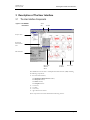
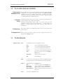


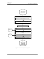
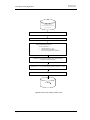
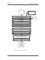
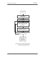
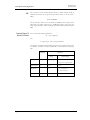
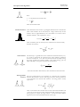

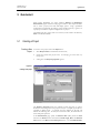
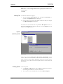
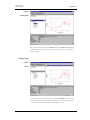
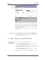
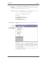
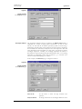
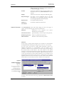
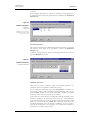
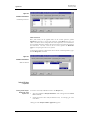
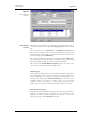
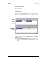
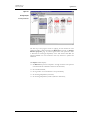
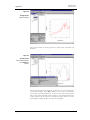
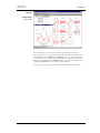


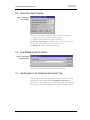
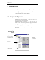
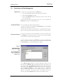
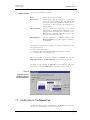
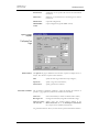
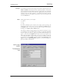
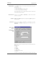
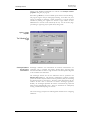
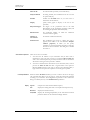
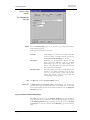
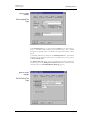
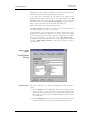
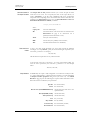
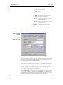
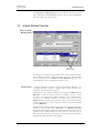
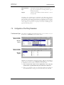
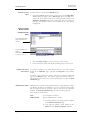
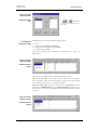
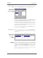
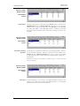
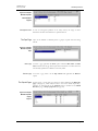
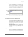
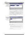
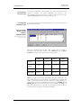
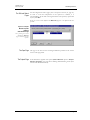

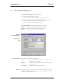
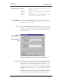
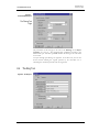

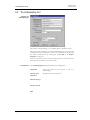

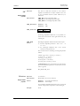






![[U4.52.03] Opérateur MODE_ITER_SIMULT](http://vs1.manualzilla.com/store/data/006360204_1-9848c5c379c7a4dd62a03820a78ec9c9-150x150.png)


![[U4.64.02] Opérateur DEFI_BASE_MODALE](http://vs1.manualzilla.com/store/data/006365607_1-b40ffc4af725e80a7c2107f2572086f5-150x150.png)