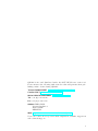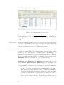
1
Belgian Institute for Space Aeronomy QDOAS Software user manual Thomas DANCKAERT Caroline FAYT Michel VAN ROOZENDAEL Isabelle DE SMEDT Vincent LETOCART Alexis MERLAUD Gaia PINARDI Version 2.109 - April 2015 QDOAS is free and distributed under the GNU GPL license version 2.0. Please mention the following authors in the acknowledgements when publishing results obtained using QDOAS. Thomas DANCKAERT [email protected] Caroline FAYT [email protected] Michel VAN ROOZENDAEL [email protected] Tel. +32 (0) 2 373 04 16 Fax +32 (0) 2 374 84 23 Address BIRA-IASB Avenue Circulaire 3 1180 UCCLE BELGIUM Web http://uv-vis.aeronomie.be/software/QDOAS Users can contact us for spectra format adaptations, remarks, suggestions and technical support. 3 Contents 1. QDOAS Overview 1.1. Introduction . . . . . . . . . . . . . . . . . . . . . . 1.2. Main QDOAS features . . . . . . . . . . . . . . . . 1.3. Main differences between QDOAS and WinDOAS 1.4. Supported spectra file formats . . . . . . . . . . . . 1.5. System requirements and installation . . . . . . . . . . . . . . . . . . . . . . . . . . . . . . . . . 7 7 7 9 10 13 2. General Description of the User Interface 2.1. The user interface components . . . . 2.2. The projects tree . . . . . . . . . . . . 2.3. The observation sites . . . . . . . . . . 2.4. The symbols . . . . . . . . . . . . . . . . . . . . . . . . . . . . . . . . . . . . . . . . . . . . . . . . . . 21 21 23 24 24 3. Description of Algorithms 3.1. Differential Optical Absorption Spectroscopy 3.2. DOAS retrieval . . . . . . . . . . . . . . . . . 3.3. Wavelength calibration . . . . . . . . . . . . . 3.4. Fit parameters . . . . . . . . . . . . . . . . . 3.5. Block-diagram structure of the program . . . 3.6. Convolution . . . . . . . . . . . . . . . . . . . . . . . . . . . . . . . . . . . . . . . . . . . . . . . . . . . . . . . . . . . . . . . . . . . 27 27 28 32 33 39 44 4. Quick start 4.1. Creating a project to browse spectra . . . . . . . . . . . . . 4.2. Example : Configuration of a project for NO2 retrieval . . . 49 49 53 5. Projects and Analysis Windows Properties 5.1. Projects properties . . . . . . . . . . . . . . . . . . . . 5.2. Analysis windows properties . . . . . . . . . . . . . . . 5.3. Configuration of the fitting parameters . . . . . . . . . 5.4. Configuration of the wavelength calibration procedure . . . . 63 63 78 81 89 . . . . 95 95 99 101 103 6. The 6.1. 6.2. 6.3. 6.4. . . . . . . . . . . . . QDOAS Tools The convolution/filtering tool (convolution) The Ring tool (ring) . . . . . . . . . . . . . The undersampling tool (usamp) . . . . . . The command line tool (doas cl) . . . . . . . . . . . . . . . . . . . . . . . . . . . . . . . . . . . . . . . . . . . . . . A. Input file format 107 B. Output 113 5 C. Troubleshooting 117 C.1. Known user interface problems . . . . . . . . . . . . . . . . 117 C.2. Analysis problems . . . . . . . . . . . . . . . . . . . . . . . 117 Glossary 121 Bibliography 123 6 1 QDOAS Overview 1.1 Introduction The experience of the Belgian Institute for Space Aeronomy (BIRA-IASB) in the development and improvement of algorithms for the retrieval of trace gas concentrations goes back to the early 1990s, with atmospheric research activities using ground-based UV-Visible spectrometers aiming at the longterm monitoring of minor components involved in the catalytic destruction of the ozone layer or in anthropogenic pollution. WinDOAS, the first program developed at BIRA-IASB in 1997, knew a success story due to a friendly user interface completed with some powerful DOAS tools. This program, extensively validated through different campaigns, has been used worldwide and for many different DOAS applications (mainly for ground-based and satellite applications). QDOAS is is portable DOAS was of QDOAS supported. a cross-platform implementation of WinDOAS: the software to Windows and Unix-based operating systems whereas Windesigned only for Windows. The user interface and the engine are similar to those of its predecessor. WinDOAS is no longer QDOAS has been developed in collaboration with S[&]T, a Dutch company well-known for the development of cross-platform products and software tools for the processing of satellite measurements (BEAT, VISAN, . . . ). The graphical user interface is built on the Open-Source version of the Qt-4 toolkit, a cross-platform application framework, and Qwt libraries. QDOAS is free software distributed under the terms of the GNU General Public License; it is open source and the code is available on request by contacting the authors. This document describes the QDOAS user interface and dialog boxes for configuring the software. It completes the online help provided with the package. The algorithms that are used in the software are also summarized. The document assumes that users already have a minimum of experience with Differential Optical Absorption Spectroscopy (DOAS) applications and retrieval. 1.2 Main QDOAS features General features The main components of the Graphical User Interface (GUI) are organized in multi-page panels with a fixed arrangement and tab-switched access to the different pages; 7 The application is based on a tree structure; Large amount of files can be processed in one shot; Support different spectra file formats (see section 1.4) On line help in HTML format Visualization of spectra and the results in different tab pages; Plot Possibility to set plot contour and style; Interactive plot mode (zooming, overlay of an existing ASCII file, possibility to fix the scaling of the plot, . . . ): activated by right clicking the title of the plot ; Export of plot in different portable image formats (png, jpg) DOAS/intensity fitting modes; Analysis shift/stretch fully configurable for any spectral item (cross-section or spectrum); possibility to filter spectra and cross-sections before analysis (supported filters include Kaiser, gaussian, boxcar, Savitsky Golay. . . ); possibility to define gaps within fitting intervals (e.g. to eliminate bad pixels); possibility to fit an instrumental offset; possibility to define several configurations of spectral windows under a project; possibility to remove spikes. wavelength calibration and instrumental slit function characterization using a Non-Linear Least Squares (NLLS) fitting approach where measured intensities are fitted to a high resolution solar spectrum degraded to the resolution of the instrument. The fitting method (DOAS or intensity fitting) can be different from the method used in the analysis; Calibration And Slit Function Characterization possibility to correct for atmospheric absorption and Ring effect; supports different analytical line shapes, as described in section 3.3, page 32. possibility to calculate differential absorption cross-sections (by orthogonalization or high-pass filtering); Cross sections handling possibility to multiply cross-sections with wavelength dependent Air Mass Factors (AMFs); possibility to fix the column density of any selected species; possibility to convolve cross-sections in real time using a user defined slit function or the information on calibration and slit function provided by the wavelength calibration procedure; possibility to handle differences in resolutions between measured and control spectra; 8 Output Tools Convolution/Filtering (convolution) The output is fully configurable. Analysis results and various data related to the measurements can be saved to ASCII or HDF-EOS5 files. Specialized tools are available for the following operations: standard and I0 -corrected convolutions are supported; possibility to create an effective slit function taking into account the (finite) resolution of the source spectrum (using a FT deconvolution method); asymmetric line shapes, wavelength dependent slit functions; Ring (ring) Undersampling (usamp) Batch processing (doas cl) The ring tool calculates Ring effect cross-sections (Rotational Raman Scattering approach). This tool generates undersampling cross-sections. For batch processing of files, the powerful command line tool doas cl can be used. 1.3 Main differences between QDOAS and WinDOAS General Differences configuration files are now in XML format, meaning that WinDOAS and QDOAS configuration files are not compatible; it is recommended to start new QDOAS applications from scratch; there is a better separation of the code between the user interface and the engine (completely transparent for users); convolution, ring, undersampling and command line tools are modules completely independent from the QDOAS main user interface. This means that QDOAS comes in five independent executables or modules : • • • • • qdoas : the user interface similar to the WinDOAS one; convolution : the convolution tool; Ring : the Ring calculation tool; usamp : the undersampling calculation tool; doas cl : a powerful command line tool that applies on qdoas, convolution, Ring and usamp configuration files. convolution, ring and usamp tools manage their own configuration files and can be called either from the QDOAS user interface or from the system command line. User Interface The main sub-components of the GUI into resizable panels with a fixed arrangement; tab-switched access for project/analysis windows settings and plotted results; All the spectral windows processed in one shot and tab-switched access between the different fitting windows; 9 There is no specific processing anymore applied on file format such as MFC (directories were considered as files with multiple records by WinDOAS). Projects Properties File format selection is now out of the Instrumental page (see page 71) in order to be able to constrain the selection of the fields in the Display and Output pages. File formats are now distributed in two groups : ground-based and satellites; NASA-AMES page doesn’t exist anymore. Analysis Windows Properties Horizontal scrolling of options; Shift and stretch in nm units only; Possibility to constrain the slant column density of a molecule to the value found in a previous window (hidden option in WinDOAS). 1.4 Supported spectra file formats Satellite Measurements Spectra measured by the following satellite instruments can be processed by QDOAS : GOME (ERS-2) QDOAS supports the original ASCII file format but it is recommended to use the more suitable binary file format created by a modified version of the GDP implemented at BIRA-IASB for the automatic selection of the reference spectrum. Contact the authors for further information about this format. SCIAMACHY (ENVISAT) Routines to read the SCIAMACHY PDS file format have been kindly provided by IFE/IUP University of Bremen. SCIAMACHY Level 1C versions up to 7.04 (the SCIAL1C utility converts files from L1 to L1C) GOME2 (MetOp) QDOAS uses the Basic Envisat Atmospheric Toolbox (BEAT) library to read spectra from GOME2. The package can be downloaded from the S[&]T web site. Before using QDOAS on GOME2 spectra, BEAT should be installed and the CODA DEFINITION environment variable should be defined. QDOAS supports GOME2 Level 1B, PPF 5.0 product format version 12.0 and below. OMI (AURA) OMI spectra are read using the HDF-EOS2 library, which is based on HDF4. Ground-based Measurements The most popular file formats supported by QDOAS for ground-based measurements are : 10 SAOZ Syst`eme d’Analyse par Observation Z´enitale developed by the aeronomy lab of the CNRS (JP Pommereau, F Goutail,...), France, and largely used in the NDACC network for stratospheric total ozone and NO2 monitoring. Both PCD/NMOS 512 and EFM 1024 (SAM) formats are supported. MFC STD This ASCII format is produced by the well-known DOASIS program designed by the atmospheric research group at IUP Heidelberg, Germany and widely used in the DOAS community. It can be obtained from the following URL: https://doasis.iup.uni-heidelberg.de/bugtracker/projects/doasis/ This format can also be produced by other program or converted from other format, e.g. the Spectra Suite Ocean Optics software. QDOAS requires the size of the detector and the format of the date (for example, MM.DD.YYYY). The MFC binary format generated by DOASIS is not supported by QDOAS. With DOASIS, it is easy to run scripts that convert the MFC binary files in MFC STD format. MFC Binary, BIRA-IASB Because spectra are saved in individual files with automatic numbering, MFC STD format is not very suitable to browse spectra and for efficient automatic reference selection (zenith of the scan for MAXDOAS data). That’s why, BIRA-IASB has developed its own MFC binary format in which all spectra of a same day including dark currents and offsets measured the night are saved in a unique file. When loading a file, measurements are automatically corrected by the averaged dark currents and offsets. The MFC Std2Bin utility that converts MFC STD files in the MFC BIRA-IASB binary format is available with the QDOAS package since version 2.107. Syntax to use from command line is : MFC_Std2Bin <config file> <input file or path> <output path> where : config file : is the name of a file with some options input file or path : the name of the MFC file or path to process output path : the path where to save the data It is recommended to apply on dark current/offset files or paths before spectra. Daily output files are automatically generated using the dates of measurement. Yearly directories are created in the output path. The config file is an ASCII file including lines starting with the following keywords : date format=... spectrum=... offset=... dark=... output prefix=... : : : : : the format of the date, for example YYYYMMDD the string identifying spectra measurements the string identifying offset measurements the string identifying dark current measurements the prefix of output file name (the date in YYYYMMDD format will follow) output extension=... : the file extension to complete the output file name The program will use the strings identifying spectra, offset and dark current to attribute a measurement type number to spectra : 1 3 4 8 for for for for off axis zenith sky dark currents offsets 11 Example of config file : date format=MMDDYYYY spectrum=Measurement Spectrum offset=Offset Spectrum dark=Dark Current Spectrum output prefix=BX output extension=bin All files of 07/01/2014 will be saved in <output path>/2014/BX_20140107.bin MKZY PAK developed at the Chalmers University of Technology, Goteborg, Sweden (MANNE Kihlman and ZHANG Yan) and used in the NOVAC network. OCEAN OPTICS very simple ASCII file format developed by the spectrometers manufacturer. The ASCII File Format Other formats are specific to the different institutes that developed them. If a format is not supported by QDOAS, it should be possible to convert the files to ASCII. When the ASCII format is selected, spectra can be provided in the file one record per line (line format) or one spectral value per line (column format) or several spectra in columns (from version 2.107). According to the checked flags in the Read from file group box, the following information are expected strictly in the given order : Solar Zenith Angle Azimuth Viewing Angle Elevation Viewing Angle Date in the DD/MM/YYYY (day/month/ year) format Fractional time In the column format, angles had to be given on the same line until version 2.106. From version 2.107, the column format accepts also matrices of spectra and angles have to be given in separate lines. The file can contain several matrices of spectra but the number of columns has to be the same for all data sets. Example of ASCII file in column format : * * * * * * data set with 4 individual spectra line 1 : solar zenith angle line 2 : elevation angle (azimuth viewing angle not provided here) line 3 : date line 4 : fractional time remaining lines : spectra values 9.5007600e+01 9.3970000e+01 9.3260500e+01 9.3067300e+01 8.5000000e+01 8.5000000e+01 8.5000000e+01 8.5000000e+01 01/07/2012 01/07/2012 01/07/2012 01/07/2012 2.9940300e+00 3.1491700e+00 3.2526400e+00 3.2804200e+00 0.0000000e+00 0.0000000e+00 0.0000000e+00 0.0000000e+00 -1.8073600e+00 -5.0432300e+00 -6.7440700e+00 -4.7440500e+00 -1.4793200e+00 -3.5119500e+00 -2.1264100e+00 -9.1264000e+00 ... ... ... ... With column format, a wavelength calibration can be provided with spectra. It should be given in first column of each data set. Other examples of ASCII files supported by QDOAS are given in appendix A. 12 1.5 System requirements and installation System Requirements The GUI is built on the Open-Source version of the Qt-4 toolkit. As a result, QDOAS is portable to Windows, Unix/Linux and Mac, and the user interface is effectively the same on all platforms. The software is free and distributed under the GNU GPL version 2.0 (see http://www.gnu. org/licenses/gpl-2.0.html for further details). To obtain the software, to get support or to be notified of new releases, please register on the following page : http://uv-vis.aeronomie.be/software/QDOAS/QDOAS_Register.php Install QDOAS on Windows Windows users can download the executables and all needed dynamic libraries from a FTP server (address provided after registration). GOME2 For GOME2 applications, the CODA DEFINITION environment variable must be defined. This variable should point to the location on the filesystem where is the .codadef file that describes the file format of the GOME2 input data. In windows, it can be set via Control Panel → System → Advanced → Environment variables Install QDOAS on Linux Users who wish to use QDOAS on linux will have to compile the program from the source code, which is provided after registration. Very likely, a number of libraries must be installed as well. This section gives an overview of the installation steps. Users without administrator privileges will typically have to install QDOAS and some of the required libraries in their home directory. In the following instructions, we will assume that the user wants to install qdoas and any libraries that might need to be installed in her home directory, /home/username. Executable files will be installed in /home/username/bin, libaries and headers in /home/username/lib and /home/username/include. When you want to install the software in a different directory, you will need to replace /home/username by the directory of choice in the following instructions. In order that the operating system can find the QDOAS executable files, the /bin subdirectory must be added to the $PATH system variable. To do this, the user will add the following entry in to her shell profile (typically the file /home/username/.profile), or execute this command directly from the shell1 : export PATH=/home/username/bin:$PATH C++ compiler g++ version 4 or higher is recommended. See the compiler notes on the Qt website for further details. 1 When you execute this command from the shell, the changes are lost at the end of your session, and you will have repeat the command every time you start a new session. Adding the command to your shell profile will cause it to be executed automatically at the start of every session. 13 Qt (http://qt-project.org) Qdoas uses the Qt4 library, version 4.6 or higher. We recommend using Qt version 4.8.5, the latest release in the Qt4 series. The current version of Qdoas can not be compiled with Qt5. The easiest solution is to install the Qt packages available from your Linux distribution’s packaging system, including the headers (development packages). Alternatively, you can download the latest source package from the Qt website. Download the Qt 4.8.5 source from http://qt-project.org/ downloads and follow the installation instructions. Qwt (http://sourceforge. net/projects/qwt) Either install the Qwt development package available for your linux distribution, or install the Qwt library using the source code. To install Qwt manually, download the latest source package from the Qwt project website and unpack it in a temporary directory. The current QDOAS version requires Qwt version 6.0.2 or higher. Open a shell and change to the Qwt root directory: edit the qwtconfig.pri and change the variables according to your installation. A sysadmin will set the QWT PREFIX INSTALL to /usr/local, while a regular user will set it to /home/username. Once the changes are made accordingly to your installation, run the command qmake qwt.pro followed by make and finally make install. This will build the Qwt libraries and install the development package (headers, documentation and runtime libraries). BEAT (http: //www.stcorp.eu/beat) QDOAS uses the BEAT library developed by the Dutch private company S[&]T to read GOME2 data. BEAT is provided as an open source library and has to be linked with QDOAS during compilation. After the installation of BEAT, the environment variable CODA DEFINITION must be set as well. BEAT can be installed using the usual “configure/make/make install” procedure. From the directory where you have downloaded the BEAT library files, type $ ./configure --prefix=/home/username This configures the install script to use the directory structure we described earlier. To complete the installation, type make, which will compile the library files, and finally make install, which will copy the compiled files, headers and other resources to the right subdirectories in /home/username. To use QDOAS with GOME2 files, you should define the environment variable CODA DEFINITION. This variable should contain the location of the .codadef files required by BEAT. For example: In c-shell: setenv CODA_DEFINITION "/home/username/share/beat/definitions" In bash: export CODA_DEFINITION="/home/username/share/beat/definitions" Again, it is practical to add these commands to your shell profile. 14 HDF-EOS2 QDOAS uses the HDF-EOS2 library to read OMI spectra. The HDF-EOS2 library itself relies on the HDF4 library. If these libraries are not yet available on your system, you can install them using your linux distribution’s package management system, or install them from the source code. If you want to install the libraries from source, HDF4 must be installed first. The HDF4 source code package is available from http://www.hdfgroup. org/ftp/HDF/HDF_Current/src. You can install it using the usual “configure/make/make install” procedure. To avoid a conflict with the HDF5 library, we have found it practical to install the HDF4 header files in a separate subdirectory. To do this, use the configure with the following arguments: $ ./configure --prefix=/home/username \ --includedir=/home/username/include/hdf4 Now, use make and make install to complete the installation of HDF4. Once you have installed the HDF4 library, download the source for HDFEOS2 from ftp://edhs1.gsfc.nasa.gov/edhs/hdfeos/latest_release/. The library comes with an installation script, but we recommend installing it with the same “configure/make/make install” procedure, which is also available. If you installed HDF4 according to the previous instructions, the following command should allow you to install HDF-EOS2: $ ./configure --prefix=/home/username CC=/home/username/bin/h4cc \ --enable-install-include When configure has finished its job, run make and make install. HDF-EOS5 QDOAS can write output data in the HDF-EOS5 format, for which it needs the HDF-EOS5 and HDF5 libraries. Again, if these libraries are not installed on your system yet, you can either install the appropriate packages for your linux distribution, or compile the libraries from source yourself. To install the libraries from source, you should first install the HDF5 library. Source code packages are available from http://www.hdfgroup. org/ftp/HDF5/current/src. The installation follows the standard “configure/make/make install” procedure. When running configure, specify the --prefix as before: $ ./configure --prefix=/home/username Again, run make and make install to complete the installation. After installing HDF5, you can obtain the HDF-EOS5 source code2 at ftp: //edhs1.gsfc.nasa.gov/edhs/hdfeos5/latest_release. This package can then be installed using configure and make. Again, you should set --prefix=/home/username to install the library at the correct location. Additionally, you need to add the option --with-hdf5=/home/username, so the installation script can find the HDF-5 libraries installed in the previous step, and --enable-install-include, in order to copy the HDF2 The current version 1.14 of the HDF-EOS5 source code contains a bug. Until a fixed version of the HDF-EOS5 library is available, we recommend also applying the patch “strcpy-overlap.patch” contained in http://archive.ubuntu.com/ubuntu/pool/ universe/h/hdf-eos5/hdf-eos5_5.1.13.dfsg.1-3ubuntu1.debian.tar.gz to the downloaded HDF-EOS5 source code. 15 EOS5 header files to the directory /home/username/include, where the Qdoas install script expects them: $ ./configure --prefix=/home/username --with-hdf5=/home/username \ --enable-install-include Complete the installation of HDF-EOS5 by running make and make install. QDOAS The QDOAS build configuration uses the Qt utility qmake. The configuration file is Src/all.pro, and it assumes that Qwt is installed in the default location – edit the file Src/config.pri to change this. Typically, the unix section of config.pri contains the following values: INSTALL_PREFIX = /home/username INCLUDEPATH += $$INSTALL_PREFIX/include INCLUDEPATH += $$INSTALL_PREFIX/include/hdf4 INCLUDEPATH += /usr/include/qwt QMAKE_RPATHDIR += $$INSTALL_PREFIX/lib QMAKE_LIBDIR += $$INSTALL_PREFIX/lib This configuration assumes that the BEAT, HDF4, HDF-EOS2, HDF5 and HDF-EOS5 libraries were installed at the location /home/username, that Qwt header files are installed at /usr/include/qwt, and that the user wishes to install the QDOAS executable files in /home/username/bin. When some of the include files and/or libraries are installed in other locations, you should add the include files’ and library files’ directories to the variables INCLUDEPATH and QMAKE RPATHDIR/QMAKE LIBDIR respectively. If you followed the instructions so far, you should only need to change /home/username to your actual username in order to install Qdoas. When you have adapted config.pri, go to the Src directory of the QDOAS source distribution. Run the command qmake all.pro followed by make. This will create the executable files, qdoas, doas cl, convolution, ring and usamp. The command make install copies the executable files to the directory $$INSTALL PREFIX/bin. QDOAS uses the Qt resource system so that the executable only depends on system Qt and Qwt libraries. The executable can therefore be safely moved to another directory. To rebuild QDOAS after an update of the package, run the following commands from the Src directory: $ make distclean $ qmake all.pro $ make Install QDOAS on MAC As BIRA-IASB doesn’t have experience with MAC systems, we present the following guidelines which have been kindly provided by two different users. Warm thanks to Will and Anoop. 1. Make sure you have Xcode installed. This comes on the DVDs included with the Mac, or the Apple developer website. QDOAS build details on Mac OS X 10.6 2. Qt and Qwt can be built separately, but allowing MacPorts (http: //www.macports.org/install.php) to do it for you is much easier - it will automatically pull in the required dependencies. sudo port selfupdate sudo port install qt4-mac sudo port install qwt-60 16 3. Install BEAT as per S&T instructions 4. Get QDOAS source (svn address provided after registration) cd trunk/Src 5. Edit config.pri to reflect the paths on your system, if using MacPorts; they will be something like : QWT_INC_PATH = /opt/local/include/qwt QWT_LIB_PATH = /opt/local/lib QWT_LIB = qwt INSTALL_PREFIX = /usr/local/Qdoas CODA_LIB_PATH = /usr/local/lib CODA_INC_PATH = /usr/local/include 6. /opt/local/bin/qmake -spec macx-g++42 all.pro make 7. If it fails on make, so we then go into the individual QDOAS program folders, e.g.: cd qdoas g++-4.2 -headerpad_max_install_names -Wl,-rpath Wl,/opt/local/lib -Wl,-rpath -Wl,/usr/local/lib -arch x86_64 -Xarch_x86_64 -mmacosx-version-min=10.6 -o +../../qdoas/release/qdoas.app/Contents/MacOS/qdoas *.o L/opt/local/lib -lqwt -L/usr/local/lib -lcoda -lm -lQtXml -lQtGui -lQtCore sudo make install Another experience with MAC 1. Check whether you are working on 32 bit of 64 bit architecture. Change this accordingly in src/all.pro, e.g. : CONFIG += ordered -arch x86_64 2. Darwin does not allow for -Wl and -rpath, you need to change this in all your .pro files in the src folder. E.g. in the gui.pro file, change the unix dependency to unix { INCLUDEPATH += /usr/local/qwt/include ../engine LIBS += -L/usr/local/qwt/lib -lqwt -lm QMAKE_LFLAGS += -rpath=/usr/local/qwt/lib } 3. Link of the binaries to the library needs to be done in the config.pri file, so I changed the unix dependency to: unix { QWT_INC_PATH = /usr/local/qwt/include QWT_LIB_PATH = /usr/local/qwt/lib QWT_LIB = qwt DYLD_LIBRARY_PATH=/usr/local/qwt/lib INSTALL_PREFIX= /Users/userName/Documents/installed_programs/qdoas/app CODA_LIB_PATH = /usr/local/lib CODA_INC_PATH = /usr/local/include # for trace-write debugging ... DEFINES += DEBUG DEFINES += LVL4 CONFIG += x86_64 } 4. Finally, once you compile it, hopefully without any problems, the app will still not work from the finder. It will however work from the terminal. If you want to make sure that the app runs in the finder by double clicking, you need to change the framework in its resources (right click: package contents). 17 // copy library into bundle: mkdir DupsApplication.app/Contents/Frameworks cp /usr/local/qwt-6.0.2/lib/libqwt.6.dylib \ DupsApplication.app/Contents/Frameworks/ // change library: install_name_tool \ -id @executable_path/../Frameworks/libqwt.6.dylib \ DupsApplication.app/Contents/Frameworks/libqwt.6.lib // change executable: install_name_tool \ -change libqwt.6.dylib \ @executable_path/../Frameworks/libqwt.6.dylib \ DupsApplication.app/Contents/MacOS/DupsApplication ---------- run these commands---------sudo mkdir qdoas.app/Contents/Frameworks sudo cp /usr/local/qwt-6.0.2/lib/libqwt.6.dylib \ qdoas.app/Contents/Frameworks/ sudo install_name_tool \ -id @executable_path/../Frameworks/libqwt.6.dylib \ qdoas.app/Contents/Frameworks/libqwt.6.dylib sudo install_name_tool \ -change libqwt.6.dylib \ @executable_path/../Frameworks/libqwt.6.dylib \ qdoas.app/Contents/MacOS/qdoas sudo mkdir convolution.app/Contents/Frameworks sudo cp /usr/local/qwt-6.0.2/lib/libqwt.6.dylib \ convolution.app/Contents/Frameworks/ sudo install_name_tool \ -id @executable_path/../Frameworks/libqwt.6.dylib \ convolution.app/Contents/Frameworks/libqwt.6.dylib sudo install_name_tool \ -change libqwt.6.dylib \ @executable_path/../Frameworks/libqwt.6.dylib \ convolution.app/Contents/MacOS/convolution sudo mkdir ring.app/Contents/Frameworks sudo cp /usr/local/qwt-6.0.2/lib/libqwt.6.dylib \ ring.app/Contents/Frameworks/ sudo install_name_tool \ -id @executable_path/../Frameworks/libqwt.6.dylib \ ring.app/Contents/Frameworks/libqwt.6.dylib sudo install_name_tool \ -change libqwt.6.dylib \ @executable_path/../Frameworks/libqwt.6.dylib \ ring.app/Contents/MacOS/ring sudo mkdir doas_cl.app/Contents/Frameworks sudo cp /usr/local/qwt-6.0.2/lib/libqwt.6.dylib \ doas_cl.app/Contents/Frameworks/ sudo install_name_tool \ -id @executable_path/../Frameworks/libqwt.6.dylib \ doas_cl.app/Contents/Frameworks/libqwt.6.dylib 18 sudo install_name_tool \ -change libqwt.6.dylib \ @executable_path/../Frameworks/libqwt.6.dylib \ doas_cl.app/Contents/MacOS/doas_cl sudo mkdir usamp.app/Contents/Frameworks sudo cp /usr/local/qwt-6.0.2/lib/libqwt.6.dylib \ usamp.app/Contents/Frameworks/ sudo install_name_tool \ -id @executable_path/../Frameworks/libqwt.6.dylib \ usamp.app/Contents/Frameworks/libqwt.6.dylib sudo install_name_tool \ -change libqwt.6.dylib \ @executable_path/../Frameworks/libqwt.6.dylib \ usamp.app/Contents/MacOS/usamp Online Help Online help is available as HTML pages. The content is similar to chapters 3, 5 and 6 of this document. HTML files have to be copied on your disk (usually a subfolder Help of the directory where executables are installed on Windows systems; a dedicated subfolder of your system share directory on Linux systems). The HTML pages are reachable from the Help button of the configuration dialog boxes. If the page can not be found, the root path of the index.html file is requested and the Help button has to be clicked again. 19 2 General Description of the User Interface 2.1 The user interface components QDOAS is based on the notion of projects. A project is as a set of files sharing the same configuration of analysis, i.e. the definition of spectral windows and the list of files to be analysed with this configuration. QDOAS allows defining several projects in a session, giving users the possibility to handle several analysis configurations. QDOAS user interface and dialog boxes are very similar to WinDOAS but now, the main components are distributed into three resizable panels with a fixed arrangement : the elements of the application organized in tree structures presented in three tab pages (Projects, Sites and Symbols) in the upper-left one; dialog boxes for the configuration of the elements of the application and the plot of spectra and results in the upper-right one; all the spectral windows are processed in one shot; right and bottom tabswitched access possible between all these pages; 21 the available information on the current spectrum and analysis results are displayed in the third one; The Menu Bar File Usual option to create a new application, open an existing one or save the current settings. QDOAS configuration files are in XML format. WinDOAS configuration files (*.wds) are not compatible with QDOAS. Plot New option to organize the plots on the page (see below), to print the plot page or to save it in a png file; Tools The Convolution, Ring and undersampling tools, already present in WinDOAS, are now modules completely independent from the QDOAS application but they can still be called from the user interface; Help Access to on-line help The Toolbar The toolbar gives access to the same File and Plot options of the menu bar. It contains also buttons to move easily in the current file or to use another file in the case a multiple files selection has been performed. Plot Properties This dialog box allows selecting a different color and a different line thickness for curves 1 and 2 (respectively the spectrum and the reference or the observed optical depth and the calculated optical depth). The number of plot columns impacts the size of the plots. Handling plots It is not possible to display a specific plot in another window as it was in WinDOAS but zoom can be made by right-clicking the Interactive option from the title of a plot. 22 The Save As option saves the plotted curves in a ASCII file (useful for example to create a reference spectrum). Export As image exports the selected plot in a png file while Print sends it to printer. Overlay will load a spectrum from a given file and superpose it over the already plotted curves but this option is not yet implemented. 2.2 The projects tree The organisation of projects, analysis windows, spectra files and directories in a tree structure completed with the definition of right-click shortcut menus at each level of the tree makes the access, manipulation and configuration of all these objects very easy. Raw Spectra Spectra to analyze have to be inserted under this projects tree node. Individual files and complete directories structures are accepted. The “New Folder” option allows organizing spectra files and directories within a userdefined catalog (folder that is not physically present on the disk). The following actions can be performed from any node: Browse Spectra browses spectra in the selected file(s); Run Analysis analyses spectra using the configuration of the project and analysis windows; this step includes the correction of the wavelength calibration of the reference spectrum if it has been requested in the configuration of the analysis windows; Run Calibration uses the options defined in the Calibration page of Projects properties (see page 69) to apply it on spectra. To move from one record to the other or from one file to the other (in case of multiple files selection), use the adequate buttons in the toolbar: Other options : Analysis windows Disable/Enable Disables the selected file or directory from the list of files to browse/analyze. Enable option re-enables previously disabled files. Refresh Refreshes the list of files in the selected directory; Show/Hide Details Shows/hides file information (last modification date and time, size). The file size information is useful to indicate if the selected file is empty or not. A project can include several spectral analysis windows. A specific analysis window can be disabled in order not to process it without removing it from the list. The View Cross Sections option is useful to check that the requested cross-sections files exist. 23 2.3 The observation sites In the Observation Sites page, a list of observation sites can be specified by their location coordinates: QDOAS applies the following conventions : longitudes are positive eastwards; negative westwards; latitudes are positive northwards; negative southwards. For ground-based measurements, information on the observation site can help to [re-]calculate the solar zenith angle as far as the measurement date and time are correct (see the Instrumental page of Projects properties, page 71). The longitude is also accounted to correctly select the reference spectrum of the day using the local time instead of the UT time in the case fractional days and times given in UT are distributed on two days (for example, for China data, two reference spectra could be selected for data of a same day before and after 00:00 UT if the observation site is not specified). For satellite measurements, this page can be used to define a list of overpasses (see the Selection page of Projects properties, page 65). In both cases, the Abbreviation is used as prefix of the name of the output files when the automatic creation of the output file name is requested. The Altitude information is just for the user. 2.4 The symbols Before configuring the analysis, the user must define the list of all relevant symbols that will be used. These symbols are needed to build cross-sections files filters, to link AMF and cross-section files and for internal manipulations (Molecules and Shift and Stretch pages of Analysis Windows properties). 24 Cross-sections symbols can be completed with a short description. The deletion of a symbol is possible only if this symbol is not used in the configuration of a project or an analysis window. 25 3 Description of Algorithms This chapter summarizes the main features of QDOAS and describes the structure of the program and the algorithms. 3.1 Differential Optical Absorption Spectroscopy DOAS is a widely used inversion method for the retrieval of atmospheric trace gas abundances from multi-wavelength light measurements. It uses the structured absorption of many trace gases in the UV, visible and nearinfrared spectral ranges. The DOAS method was originally developed for ground-based measurements (Platt [17]; Platt and Stutz [18]) and has been successfully adapted to nadir measurements from UV-Vis space-borne spectrometers (Gottwald et al. [9]). It relies on the application of the BeerLambert law to the whole atmosphere in a limited range of wavelengths. The Beer-Lambert law states that the radiant intensity traversing a homogeneous medium decreases exponentially with the product of the extinction coefficient and the path length. Applying this law to the atmosphere, we obtain n X I(λ) = I0 (λ) exp − S j (λ)cj , (3.1) j=1 where I0 is the spectrum at the top of the atmosphere, without extinction; I is the measured spectrum after extinction in the atmosphere; S j is the absorption cross section of the species j, with wavelength dependent structures [cm2/molec.]; cj is the column density of the species j [molec./cm2]. The logarithm of the ratio of the spectrum I0 (also called the control spectrum) and the measured spectrum I is denoted optical density (or optical thickness) τ X n I0 (λ) τ ≡ ln = S j (λ)cj . (3.2) I(λ) j=1 The key idea of the DOAS method is to separate broad and narrow band spectral structures of the absorption spectra in order to isolate the narrow trace gas absorption features. In order to do this, some approximations are made: 27 1. In the case where the photon path is not defined (scattered light measurements), the mean path followed by the photons through the atmosphere up to the instrument is considered; 2. The absorption cross sections are supposed to be independent of temperature and pressure, which allows us to introduce the concept of Slant Column Densities (SCDs); 3. Broadband variations, such as loss and gain from scattering and reflections by clouds and/or at the earth surface, are approximated by a common low order polynomial. Molecular absorption cross sections are fitted to the logarithm of the ratio of the measured spectrum and the reference spectrum (i.e. an extraterrestrial irradiance spectrum for satellite measurements, or a spectrum measured around the local noon when the light path is minimum for ground-based measurements). The resulting fit coefficients are the integrated number of molecules per unit area along the atmospheric light path for each trace gas, the differential SCD. The slant column depends on the observation geometry, the position of the sun and also on parameters such as the presence of clouds, aerosol load and surface reflectance. 3.2 DOAS retrieval DOAS fitting In the DOAS analysis, high frequency spectral structures of the various absorbing species are used to resolve the corresponding contributions to the measured optical density. This is achieved using a least squares fitting procedure for the differential slant column densities of the various species. Large band contributions to the atmospheric attenuation (Rayleigh and Mie scattering) are accounted for by including a low order polynomial P k P (λ) = bk λ in the fit. Other effects, such as the Ring effect or instrument undersampling can be treated as pseudo-absorbers. According to eq. (3.2), the DOAS retrieval is a linear problem. This linearity is unfortunately broken down by the need to account for additional effects, namely: 1. small wavelength shifts ∆(λ) between I and I0 spectra must be corrected using appropriate shift and stretch parameters; 2. possible instrumental and/or atmospheric stray light or residual dark current signal require the introduction of an offset parameter. Including these necessary non-linear corrections and the polynomial component P (λ), we obtain the modified equation X n I(λ + ∆(λ)) − offset(λ) ln + S j (λ)cj + P (λ) = 0 . (3.3) I0 (λ) j=1 Marquardt-Levenberg Algorithm The SCDs cj can be retrieved by performing a least squares fit of the measurement data to equation (3.3). Due to the shift, stretch and offset parameters, this is a non-linear least squares problem, which can typically be solved using a Marquardt-Levenberg (M-L) algorithm (see Marquardt [15]; Bevington [2]). Starting from given initial values, this algorithm searches the parameter space using a combination of Gauss-Newton 28 and gradient descent steps. The M-L algorithm is an efficient minimization algorithm for a wide range of non-linear functions, but it may converge to a local minimum if the initial values are too far from the global minimum. In QDOAS, this problem can occur during the wavelength calibration, when the initial calibration is not accurate enough (see Calibration problems in section C.2 of the appendix). In QDOAS, the M-L algorithm is used to find the set of parameters that minimizes the weighted1 sum of squares M 1X F (~ α) = 2 i=1 M 1X = 2 f i (~ α) σi 2 ln(I i (~a)) + Pn j=1 S ij c j + Pd k k=0 bk (λi ) − ln(I0i ) σi i=1 !2 , (3.4) where α ~ = (~a, ~b, ~c) is the vector containing all fitted parameters; ~a is the set of parameters describing the shift, stretch and offset of the measured spectrum; bk , k = 1, . . . , d are the fitted polynomial coefficients; cj , j = 1, . . . , n are the fitted SCDs; λi , i = 1, . . . , M is the wavelength grid of the reference spectrum I0 , calibrated with respect to a high resolution solar spectrum (see section 3.3). I i (~a) is the measured spectrum, including shift, stretch and offset corrections, interpolated at wavelength λi ; S ij is the absorption cross section of absorber species j, as measured in a laboratory, interpolated at wavelength λi ; I0i is the reference spectrum at wavelength λi and σ i is the standard error on the measurement at wavelength λi . In each iteration, the fitting algorithm will choose new values for the parameters using the Marquardt-Levenberg algorithm, and recompute the sum of squares F . The algorithm assumes that it has converged to a solution when the difference between two succeeding values of F is smaller than a fixed small number . The convergence criterion can be chosen by the user (see Convergence Criterion in section 5.1). For a given value of the non-linear parameters ~a, the determination of the parameters cj and the polynomial coefficients bk is a linear least squares problem. Explicitly, we can rewrite equation (3.4) as M F = 1X 2 i=1 1 ln(I i (~a)/I0i ) + (A · ~x)i σi 2 , (3.5) Weighting the residuals by the instrumental errors σ i is optional in QDOAS. When no measurement uncertainties are used (or no error estimates are available), all uncertainties in equation (3.4) are set to σ i = 1, giving all measurement points equal weight in the fit. See analysis properties in section 5.1 29 where the matrix A contains the polynomial basis (λi )k , k = 0, . . . , d and the absorption cross sections S ij , j = 1, . . . , n and ~x represents the combined linear parameters ~b and ~c: Ail = (λi )d S ij , (3.6) ~b ~x = . (3.7) ~c This fact is exploited in QDOAS to limit the parameter space of the ML algorithm to the non-linear parameters: once a new set of values ~a0 for the non-linear parameters is chosen, the linear parameters bk and cj are updated using a linear least squares algorithm, minimizing the sum of squares (3.4) for the given values of the non-linear parameters. In QDOAS, the linear least squares problem is solved using the Singular Value Decomposition (SVD) of the matrix A defined in equation (3.6). QDOAS can include further parameters in the fits (3.4), which we omitted from the previous description for the purpose of clarity. Such parameters include the width of the instrument’s slit function and wavelength shifts in the reference absorption cross sections S j (λ). Mathematically, they play the same role as the shift, stretch and offset parameters ~a. Section 5.3 describes the available fitting options in QDOAS and their configuration. Intensity fitting QDOAS also supports the so-called intensity fitting (or direct fitting) method where measured intensities are directly fitted instead of their logarithms. The equation used in the least squares fitting procedure is then n X I(λ + ∆(λ)) − offset(λ) − P exp(− S j cj ) = 0 , I0 (λ) (3.8) j=1 This method involves a decomposition of equation (3.8) in its linear and non-linear parts: column densities are fitted non-linearly, but the polynomial, which is taken out of the exponential function using a Taylor expansion, and offset are linear parameters. Intensity fitting is sometimes preferred to optical density fitting, for example when a poor signal leads to numerical problems when taking the logarithms of the intensity ratio. Errors On Slant Column Densities Uncertainties on the retrieved slant columns cj depend on: the sensitivity of the sum of squares F (3.4) with respect to variations of the fitted parameters around the minimum and the noise on the measurements. Formally, the covariance matrix of the fitted parameters of a least squares estimate may be estimated by the inverse of the Hessian of the sum of squares F , evaluated at the fitted values of the parameters Σα~ = H −1 , (3.9) where H is given by Hkl = 30 ∂2F . ∂αk ∂αl (3.10) The actual approach used to calculate H in QDOAS is different in optical density fitting mode and in intensity fitting mode. In optical density fitting mode, the slant column density is fitted linearly according to equation (3.5) and we use the following expression for the covariance matrix Σ~x of the weighted linear least squares parameter estimate: Σ~x = AT W 2 A −1 , (3.11) where the matrix A contains the linear components of the fit, as described in equation (3.6) and the (M × M ) diagonal matrix W contains the measurement errors 1 (3.12) Wij = i if i = j . σ Equation (3.11) implies that uncertainties on estimated values of the nonlinear parameters are not taken into account in the reported errors on the slant columns. When the individual measurement errors σ i are not available (or the user has chosen not to weight the fit by the instrumental errors), the weight matrix W is just the identity matrix. In this case, the mean squared error on the measurements σ 2 may be estimated by the reduced χ2 , e.g. the sum of squares of the residuals divided by the number of degrees of freedom in the fit PM (f i )2 2 χ = i=1 , (3.13) M −N where M is the number of wavelengths included in the fit, and N is the total number of fitted parameters. Equation (3.11) then becomes −1 . Σ~x = χ2 AT A (3.14) In intensity fitting mode, the slant column densities are determined using non-linear least squares fitting, and the Hessian is approximated by the square of the Jacobian of the fitting functions f i Hkl ' M X ∂f j ∂f j 1 . ∂αk ∂αl (σ j )2 (3.15) j=1 This implies that, in intensity fitting mode, uncertainties on the linear parameters are not taken in to account in the reported slant column errors. As in the linear case, when the instrumental errors are not used or not available, the σ j in equation (3.15) are replaced by 1, and the measurement error is approximated using the reduced χ2 of the fit instead. Equation (3.9) then becomes Σα~ = χ2 H −1 . (3.16) Limitations The estimates for the uncertainties of the fitted parameters rely on the statistical model used for the DOAS retrieval. The model assumes that the errors on the measurements at each frequency are independent and normally distributed. When measurement errors are correlated or contain systematic components, or in case of fitting errors such as a wrong fit for shift and stretch parameters, or relevant absorbers that are not included in the fit, the uncertainties calculated by QDOAS will underestimate the 31 true error on the slant column density. Remaining residual structures after the fit, or a value of χ2 1 when measurement errors σ i are taken into account, are an indication of such a bad fit. A discussion can be found in Stutz and Platt [23]. We also note that the errors in QDOAS do not take into account the uncertainties on the cross sections. A way to achieve this is given in Theys et al. [24]. 3.3 Wavelength calibration The quality of the retrieval fit strongly depends on a perfect alignment between the spectrum to analyze, the reference spectrum and the cross sections. The wavelength-pixels relation (see Platt and Stutz [18]) of the reference spectrum, previously determined in laboratory using a lamp spectrum can be corrected using a procedure based on the alignment of the Fraunhofer structures of the reference spectrum I0 with those of an accurately calibrated high-resolution solar reference atlas, degraded at the resolution of the instrument, i.e. convolved with the instrumental slit function. The reference atlas used for this purpose is usually the Chance and Kurucz [7] spectrum. During the calibration process, the instrumental slit function can also be characterized by repeatedly convolving the highly resolved solar atlas with the slit function and adjusting the parameters until the best match with the reference spectrum is found. QDOAS allows fitting the parameters of different line shapes, as well as their wavelength dependence. This is useful when the slit function provided with the instrument is not described precisely enough in the wavelength interval used for the retrieval. In the same way, to account for the moderate resolution of satellite or ground-based instruments (about a few tenths of a nanometer), the absorption cross sections of the trace gases have to be convolved with the instrumental slit function (and interpolated on the final I0 wavelength grid). A good knowledge of the instrumental slit function and its potential wavelength variation is important to avoid systematic errors in the retrieved slant columns due to spectral shape mismatch between the reference and atmospheric spectra [25]. Fit of shift and stretch Shift and stretch (see Shift on page 35) can be taken into account in the wavelength calibration scheme. To this end, the spectral interval is divided into a number of equally spaced sub-intervals. The fitting algorithm used for the DOAS retrieval is then applied in each sub-interval to fit the measured intensities to those of the high-resolution solar spectrum, according to the equation I0 (λ) = IS (λ − ∆i ) exp(− m X S j cj ) , (3.17) j=1 where IS is the solar spectrum convolved at the resolution of the instrument, ∆i is a fitted constant shift in sub-interval i, and the cj are optional absorber coefficients accounting for possible light absorption in the reference spectrum I0 . A value of the shift ∆i is calculated in each sub-interval 32 i and a polynomial is fitted through the individual points in order to reconstruct an accurate wavelength calibration ∆(λ) for the complete analysis interval. Several tests may be needed to determine the best configuration. One has to find the right compromise between using enough sub-intervals to represent the wavelength variation of the shift, and having enough spectral information in each sub-window. The interval calibration should cover all analysis spectral windows. The algorithm can take into account molecular absorption and offset correction. In order to help the algorithm to converge to the exact solution, it is important to start with a preliminary wavelength grid close enough to the real one and to limit the number of fitting parameters (for example by fixing the value of some parameters, typically the concentration of the fitted molecules after a first estimation). Ref2/Ref1 Alignment If two reference spectra are given (see section 5.1 and figure 5.17), the wavelength calibration described in the previous section is applied to the first one. The shift between both reference spectra is then determined using a least squares fit. This shift is then applied to the reference absorption cross sections in order to align them on the second reference spectrum. The measured spectra are then analyzed with respect to the second reference spectrum. Characterization Of The Line Shape If the slit function varies strongly in the fitting window and is symmetric enough to be approached by an analytical function like a Gaussian, it can be fitted together with the shift during the calibration procedure. A high resolution solar spectrum is needed. The wavelength variation of the line shape can be accounted for in order to convolve high-resolution cross sections before the analysis. The equation (3.17) used in the calibration is then modified as follows: m X I0 (λ) = (Lai ∗ IS )(λ − ∆i ) exp − cj S j , (3.18) j=1 where Lai (λ) is the line shape with Full Width at Half Maximum (FWHM) parametrized by ai . QDOAS can fit the parameters for a number of different analytical line shapes, which we describe in more detail in the Analytical line shapes section on page 44. 3.4 Fit parameters Absorption cross sections In principle, DOAS measurements are applicable to all gases with suitable narrow absorption bands in the UV, visible or near IR regions. However, the generally low concentrations of these compounds in the atmosphere and the limited signal-to-noise ratio of the spectrometers restrict the number of trace gases that can be detected. Figure 3.1 shows the absorption cross sections of a number of trace gases that are regularly measured using the DOAS technique. 33 Figure 3.1.: Absorption cross sections of various absorbers retrieved with the DOAS method (figure taken from Platt and Stutz [18]). Many spectral regions contain a large number of interfering absorbers. In principle, because of their unique spectral structure, a separation of the absorption is possible. However, correlations between absorber cross sections sometimes lead to systematic biases in the retrieved slant columns. In general, the correlation between cross sections decreases if the wavelength interval is extended, but doing so is at odds with the assumption that a single effective light path for the entire wavelength interval is defined, leading to systematic misfit effects that may also introduce biases in the retrieved slant columns. To optimize DOAS retrieval settings, a trade-off has to be found between these effects. A basic limitation of the classical DOAS technique is the assumption that the atmosphere is optically thin in the wavelength region of interest. At shorter wavelengths, the usable spectral range of DOAS is limited by rapidly increasing Rayleigh scattering and O3 absorption. In addition, ‘line-absorbers’ such as H2 O, O2 , CO, CO2 and CH4 usually cannot be retrieved precisely by standard DOAS algorithms because their strong absorption also depends on pressure and temperature. The selection of the spectral analysis window determines which absorbers have to be included in the fitting procedure. The pressure dependence of absorption cross sections can be neglected in UV-Visible region. However, the temperature dependence of cross sections can be significant (for example that of O3 and NO2 ). This can be corrected in a first approximation by introducing correction factors during the AMF calculation [3] or, assuming a linear dependence on temperature, by fitting two absorption cross sections at different temperatures as described in Van Roozendael et al. [25]. 34 Figure 3.2.: Cross section O3 and optical thickness τ are separated into a narrow (O03 and τ 0 ) and a broad band part (O3p and τp ) by an adequate filtering procedure. Shift Before analysis, absorption cross sections are interpolated on the final grid of the reference spectrum which may be determined by the program itself (automatic reference selection mode). Moreover, shift and stretch parameters can be fitted during the processing of a spectrum in order to obtain the best match of the absorption structures. Interpolation/Convolution Cross sections can be pre-convolved and interpolated2 on an appropriate wavelength grid prior to the analysis. However, the direct use of highresolution cross sections which can be convolved in real-time with a predefined slit function or with the slit function determined by the wavelength calibration procedure, is more convenient. Differential cross sections The aim of calculating differential absorption cross sections is to separate narrow spectral features from unstructured absorption not useful in the DOAS method. Figure 3.2 gives an illustration. Differential cross sections can be calculated by orthonormalization with respect to an orthogonal set formed with the low order component vectors (usually a base of order 2 or 3) of the polynomial. The vectors are orthogonalized using the Gram-Schmidt algorithm. This method gives also the possibility to separate the spectral structures of temperature dependent cross sections by mutually orthogonalizing them. Differential cross sections can alternatively be obtained by high-pass filtering: a filter is applied iteratively on the cross section and the resulting cross section is subtracted from the original one. High-pass filtering is presently only supported in optical density fitting mode (DOAS mode). Note that it is not necessary to calculate differential cross sections when the baseline is around 0 such as for H2 O, O4 or H2 CO. Low-pass filtering Low-pass filters can be applied to both spectra and absorption cross sections. A large choice of filters is proposed (see ‘Filtering Page’, section 5.1). 2 By default, QDOAS uses cubic spline interpolation. 35 Wavelength-dependent AMF Absorption cross sections can be replaced by geometrically corrected cross sections that take into account the wavelength dependency of the AMF. The correction is based on the equation ln(I0 ) − ln(I) = S(λ)AMF(λ, SZA) , (3.19) where AMF(λ, SZA) is the AMF calculated for a given wavelength λ and a given Solar Zenith Angle (SZA). Polynomial In the DOAS technique, absorption cross sections of the considered molecules are highly structured, while scattering by molecules and particles (Rayleigh and Mie scattering), as well as reflection at the surface, have broadband dependencies that can be approximated by a low order polynomial. In QDOAS, polynomials up to degree 5 can be fitted. The low order components of the polynomial can be used to calculate differential cross sections when this is preferred to high-pass filtering. Shift and Stretch Shift and stretch parameters allow to correct possible misalignment between the various wavelength-dependent quantities involved in the data evaluation (i.e. measured and reference spectra as well as absorption cross sections). Shift and stretch parameters may be fitted or simply applied to any wavelength-dependent quantity, according to the equation ∆λ = a + b(λ − λ0 ) + c(λ − λ0 )2 , (3.20) where λ is the wavelength according to the original calibration and λ0 is the center wavelength of the current spectral range. The parameters a,b and c describe the offset and the first and second order stretch applied to λ. Offset Correction An ideal spectrometer in an ideal atmosphere would measure the part of the sunlight that has been elastically scattered by air molecules and particles. In a real experiment, however, a number of possible additional sources may contribute to the measured intensity, adding an “offset” to the ideal Rayleigh/Mie contribution. In addition to the Ring effect, which is, to a first approximation, a natural source of offset, one must also account for instrumental sources of offset, such as stray light in the spectrometer and dark current of the detector. The offset component in equation (3.3) accounts for these effects. QDOAS models the offset using a polynomial offset(λ) = (a + b(λ − λ0 ) + c(λ − λ0 )2 )I¯ , (3.21) where λ0 is the center wavelength of the spectral analysis window, I¯ is the average intensity and a, b and c are fitted parameters. ¯ the offset values can be easily interpreted Due to the normalization by I, relatively to the absolute intensity of the spectrum (percent offset). In DOAS, the offset is usually fitted as a non-linear parameter. Sometimes, this could lead to numerical errors in the evaluation of the logarithm, typically in the near UV region where the level of the signal is very low. In this case, we can fit the offset as a linear parameter. Expanding the left-hand side of equation (3.3) to first order, we obtain ln(I(λ + ∆(λ))) = ln(I0 (λ)) − τ (λ) + 36 offset(λ) . I(λ + ∆λ) (3.22) Ring Effect Because of Rotational Raman Scattering (RRS), a small fraction of the incident photons undergo a wavelength change of a few nanometres, i.e. a part of the scattering is inelastic. This causes an intensity loss at their incident wavelength and a gain at the neighbouring wavelengths to which they are redistributed. RRS causes the so-called “filling-in” of Fraunhofer lines, which have a slightly different shape in the earthshine radiance than in the direct solar light. This effect was first discovered by Grainger and Ring [10] and is referred to as the Ring effect. The atmospheric absorption lines are also broadened by RRS events occurring after absorption (molecular Ring effect). Although RRS accounts for only a few percent of the measured intensity, it significantly affects DOAS measurements of scattered radiation since typical trace gas absorptions are of the order of a percent or less. If not properly corrected, the Ring effect produces strongly structured residuals in the differential optical density, due to the fact that Fraunhofer lines do not cancel perfectly between I and I0 . Especially in the UV spectral range, the remaining spectral structures can by far exceed the structures of weak atmospheric absorbers. Usually the Ring effect is taken into account by including an additional ‘absorber’ in the DOAS fit. Ring cross sections SRing (λ) can be measured [22] or calculated [8]. The Ring effect can be approximated using the following development for an optically thin atmosphere [27; 25]: One can consider that in any scattered light observation, the light detected by the satellite instrument (Imeas ) is the sum of elastic and inelastic scattering processes: Imeas = Ielastic + IRRS = I0 e−τ + IRRS . (3.23) To analyze a measured spectrum, the logarithm of Imeas is taken. Since IRRS is very small compared to Ielastic , the logarithm can be approximated by the first two terms of the Taylor expansion: ln(Imeas ) = ln(Ielastic ) + IRRS IRRS = ln I0 − τ + . Ielastic Ielastic (3.24) The last term IRRS /Ielastic is the Ring term which can be approximated by the product of a Ring coefficient αRing and a Ring cross section SRing . αRing can be fitted together with other absorbers in the DOAS procedure. A good approximation of the Ring cross section can be obtained from calculation of a source term I0Raman for Raman scattering derived by simple convolution of the solar spectrum with Raman cross sections, i.e with calculated N2 and O2 RRS cross sections. The term IRRS /Ielastic in equation (3.24) is then substituted by αRing SRing (where SRing = I0Raman /I0 ), assuming that the molecular Ring effect can be neglected [8]. The QDOAS Ring tool calculates a Ring cross section according to this approach [27]. The normalization of the Raman spectrum is optional. Undersampling Correction The undersampling is a well-known problem of GOME [6]. It arises from the poor sampling ratio of the GOME instrument, which results in a loss of spectral information when interpolating earthshine spectra during the DOAS fitting process. Undersampling is only a major problem when the sampling ratio is close to 1. In the case of GOME, this ratio is estimated at 0.16/0.112=1.43 at 340 nm. 37 The undersampling artifacts can be corrected using an ad-hoc cross section obtained by simulating the effect based on a high-resolution solar reference [6]. This cross section is fitted as a linear parameter, in both intensity fitting and in optical density fitting modes. The procedure to calculate the correction differs slightly between the two fitting modes: In intensity fitting mode, oversampled and undersampled spectra are calculated as follows: U (λ + ∆) = over(λ + ∆) − under(∆) (λ) , (3.25) where over(λ + ∆) is a high-resolution solar spectrum convolved on its original grid and interpolated on the final grid λ + ∆ and under(∆) (λ) is a high-resolution solar spectrum convolved on grid λ and subsequently interpolated on the final grid λ + ∆. Residuals are improved by adding a “second phase” of undersampling U2 (λ) = over(λ) − under(∆) (λ) . (3.26) In optical density fitting, we fit the logarithm of the ratio of the measured intensities. We therefore use the corresponding equations U (λ + ∆) = ln U2 (λ) = ln over(λ + ∆) ! under(∆) (λ) over(λ) under(∆) (λ) , (3.27) . (3.28) ! Undersampling cross sections can be pre-calculated using the QDOAS undersampling tool or they can be calculated in real time, just after the wavelength calibration procedure using the corrected wavelength grid and the characterized slit function. AMF To obtain the Vertical Column Density (VCD) from the fitted SCD, we have to divide the SCD by the AMF VCD = SCD . AMF (3.29) AMF’s are not calculated by QDOAS but may be imported from ASCII files (for details, refer to appendix A). QDOAS supports solar zenith angledependent AMF, wavelength-dependent AMF and climatological AMF. Graphical Display Of Spectral Fit Results According to the selected fitting method, different formulas are used to display the measured data and the calculated fit results. Tables 3.1 and 3.2 explain which quantities are displayed on the fit results page for optical density fitting mode and intensity fitting mode. The following quantities 38 Residual Cross sections Polynomial Offset Calculated Measured S j · cj P O Rod S j · cj + Rod P + Rod O + Rod Table 3.1.: Formulas used by QDOAS to display the results of a fit in optical density fitting mode. S j is the reference cross section for species j and cj the corresponding SCD. P (λ) is the polynomial obtained from the fit. See equations (3.30)-(3.34) for the definitions of the quantities Rod and O. Normalized Residual OD Residual Cross sections Polynomial Offset Calculated Measured S j · cj P O Rnorm Ri S j · cj + Ri Pmeas O + Ri Table 3.2.: Formulas used by QDOAS to display the results of a fit in intensity fitting mode. S j is the reference cross section for species j and cj the corresponding SCD. P (λ) is the polynomial obtained from the fit. See equations (3.30)-(3.34) for the definitions of the quantities Rnorm , Ri and O. are used: P Rod = ln P Rnorm P · I0 · e− S = I − offset Ri = ln j I0 · e− S cj −P I − offset jc ! , (3.30) j − 1, P j ! P · I0 · e− S I − offset (3.31) cj , I − offset P j , I0 · e− S cj O = ln(1 − offset/I) , Pmeas = (3.32) (3.33) (3.34) where I is the measured spectrum, I0 is the reference spectrum, P the fitted polynomial, S j the absorption cross section for absorber species j and cj the corresponding fitted concentration. 3.5 Block-diagram structure of the program The following figures give an overview of the structure of the program. Figure 3.3 describes the general organization of the processor. Figures 3.4 and 3.5 show the structure of the wavelength calibration and slant column fitting modules, while the coupled non-linear least squares fitting algorithm is sketched in Figure 3.6. 39 Initial wavelength calibration λ Control spectrum I0 (λ) Cross sections S j Pre-processing Wavelength calibration and slit function parametrisation Apply NLLS fit to high resolution Fraunhofer reference spectrum (see figure 3.4) Apply wavelength calibration Convolve and/or interpolate sigma using wavelength calibration and SFP Select fitting method Processing Spectra Load Spectra Slant columns fitting Apply a NLLS fit to deduce slant column densities AMF Interpolation of AMF on the spectra SZA Conversion of slant columns to vertical columns All fitted parameters SCD and VCD Standard Deviations Figure 3.3.: Overall structure of the spectral analysis program. 40 Initial wavelength calibration λ Control Spectrum I0 High-resolution solar spectrum Isol cross sections S j Select calibration interval and split into N sub-windows Select fitting mode (DOAS/Intensity fitting) Slant column fitting (see figure 3.5) In each fitting window n, derive: - The shift ∆n between Isol,n and I0,n - The slit function parameters SFPn - SCD of correcting absorbers (O3 , Ring, ...) Determine the new wavelength calibration by polynomial fitting through the N individual shift values ∆n Determine wavelength dependence of slit function parameters SFP(λ) by polynomial fitting through the N individual SFPn values Display calibration results (optional) Wavelength calibration SFP(λ) Figure 3.4.: Structure of the wavelength calibration module. 41 I, I0 , S j , λ, N L Cross section processing S j correction with wavelength-dependent AMF (optional) AMF(λ, SZA) Convolve/shift/interpolate S i Low-pass filtering (optional) Generate differential S j (by orthogonalisation or high-pass filtering) Spectra processing Shift I (or I0 ) Apply offset correction to measured spectrum I Decompose the fitting function into linear and non-linear components (depending on the fitting method) NLLS fit (see figure 3.6) Residual R Fitted Parameters, including SCD Standard Deviations Figure 3.5.: Structure of the slant column fitting module. Cross section processing only takes place during the pre-processing phase, unless cross sections must be dynamically modified during the fit (e.g. when fitting a cross section shift). 42 I, I0 , S j , λ I, I0 low pass and high pass filtering (optional) Initialization of non-linear parameters NLLS fit Update non-linear parameters according to MarquardtLevenberg algorithm LLS fit Minimize F (eq. (3.4)) for current values of non-linear parameters by solving the linear least squares problem n ∆F < y Residual R Fitted Parameters, including SCD Standard Deviations Figure 3.6.: Structure of the non-linear least squares fitting algorithm used in the slant column fitting module and in the wavelength calibration module. 43 3.6 Convolution Definition The convolution of a spectrum I by an instrumental slit function F is given by the integral Z (F ∗ I)(λ) = I(λ0 )F (λ − λ0 )dλ . (3.35) In QDOAS, this integral is calculated using the trapezoidal rule. The integration interval is defined by the width of the slit function. The three tools (Convolution, Ring and Usamp) provided in the QDOAS package, support convolution with one of the following functions: the Gaussian line shape, the 2n-Lorentzian line shape, the Voigt profile, the error function, an asymmetrical Gaussian line shape, a boxcar (using Fourier Transform) Norton-Beer strong (using Fourier Transform) arbitrary line shapes provided in ASCII files. Analytical line shapes QDOAS can calculate the Gaussian, Lorentzian, Voigt, asymmetrical Gaussian and error function line shapes for different values of their parameters. When one of these analytical line shapes is used, QDOAS can fit its parameters during the wavelength calibration procedure (see section 3.3, page 33). 44 (a) (b) (c) (d) (e) (f) Figure 3.7.: QDOAS can use different line shapes to describe the instrumental slit function. The plots above illustrate the Gaussian (a), asymmetrical (b, c), Voigt (d) and Lorentzian (e, f) profile shapes. The asymmetry factor in (b) is 0.2, that of line shape (c) is 0.4. The Lorentzian (e) is the standard Lorentzian (n = 1) and the Lorentzian in (f) has n = 2. In order to make the convolution algorithm faster, analytical slit functions are pre-calculated on a suitable wavelength grid (determined in order to have 18 pixels at FWHM) and then interpolated on the grid of the spectrum. For Gaussian and error function line shapes, a Fast Fourier Transform (FFT) algorithm is used whenever possible to speed up the calculation (e.g. within the wavelength calibration procedure). As a convention, QDOAS always requests the full width at half maximum (FWHM) of the line shape in the user interface. This parameter is represented by σ in the formulas below. Gaussian The standard expression used to approximate instrumental slit functions is the Gaussian function (see figure 3.7(a)). The Gaussian is the exact line shape in the diffraction limit, i.e. in the case of an infinitely thin entrance slit. The normalized Gaussian is given by 2 1 x Gσ (x) = √ exp − 2 , a a π (3.36) where a depends on the Gaussian full width at half-maximum σ as follows: √ σ = 2 ln 2a . Error function (3.37) For a large entrance slit, the slit function can be approximated by the convolution of a boxcar and a Gaussian function. The resulting slit function is given by 1 Ea (x) = 4∆ x+∆ x−∆ erf − erf , a a (3.38) 45 where a depends on the Gaussian full width at half-maximum σ (see 3.37), ∆ is half the boxcar width b and erf(x) is the error function, defined by Z x 2 exp(−t2 )dt . (3.39) erf(x) = √ π 0 Full width at half maximum of the Gaussian σ (see 3.37) and boxcar width b (2*∆) are the two parameters requested by QDOAS for the error function. 2n-Lorentzian This line shape is a generalization of the well-known Lorentzian function (n = 1, see figure 3.7(e)). It is useful to approximate slit functions with a shape significantly different from the Gaussian one. Low order 2n-Lorentz can mimic line shapes with large wings (typically the standard Lorentzian profile), or line shapes having a flat top (for higher values of n, see figure 3.7(f)). The generic expression for this function is L2n (x) = τ 2n , x2n + τ 2n (3.40) with τ = σ/2 (σ is the full width at half maximum). Parameters requested by QDOAS are the full width at half maximum of the Gaussian σ (see 3.37) and N = 2n. Voigt profile The Voigt profile function (see figure 3.7(d)) is the convolution of a Gaussian and a Lorentzian function. This function is used in a wide range of contexts, and the optimization of its computation has received much attention. The Voigt profile is usually expressed as Z y ∞ exp(−t2 ) K( x, y) = dt , (3.41) π −∞ (x − t)2 + y 2 where x is the distance from the line center in units of Gaussian half-widths and y is the ratio of the Gaussian to the Lorentzian half-width. Numerous ways have been proposed to compute the Voigt function. A rather efficient algorithm is described by Kuntz [13]. Asymmetrical Gaussian To handle asymmetrical line shapes, QDOAS can fit an asymmetry factor in addition to the FWHM. The line shape used is a modified version of the Gaussian line shape (3.36) 1 x2 0 G (x) = √ exp − 2 , (3.42) a (1 + sign(x)b)2 a π where, in addition to the FWHM σ, the asymmetry factor b is now fitted as well. For a value of b = 0, it reduces to the ordinary Gaussian line shape. Figure 3.7(b) illustrates the line shape with an asymmetry factor of b = 0.2 and 3.7(c) gives an illustration for b = 0.4. User-defined line shape An alternative to fit asymmetrical slit functions is to provide a line shape in an ASCII file and to apply on the grid of the line shape a stretch factor that can be different for each side of the line shape. The “Stretch on wavelength” file in the Convolution tool is a ASCII file with three columns : the 46 wavelength calibration and the two values of the stretch to apply on the grid of the line shape for each wavelength of the detector. Lookup tables of slit functions are also accepted. This means that a line shape is provided for different wavelengths. For a specific wavelength, a line shape is first calculated by linear 2D-interpolation in the lookup table and the fitted stretch factors are then applied to the line shape wavelength grid before convolution. Wavelength dependency QDOAS supports convolution with wavelength-dependent slit functions: Slit function files provided by the user may contain multiple columns describing the shape of the slit function at various wavelengths. The first line of the file should list the wavelengths for which the slit function is provided. QDOAS will then generate a lookup table from the provided slit functions, and calculate the slit function at intermediate wavelength values using linear interpolation. For analytical line shapes, the user can provide a two-column ASCII file containing the wavelengths and corresponding values of the parameters for each requested parameter (for example, the Gaussian width and the boxcar width for the error function). Files with the correct parameter calibration can be saved from the SFP plots obtained after the wavelength calibration procedure. For more details on how to compute such a convolution using QDOAS, see section 6.1, page 97. Correction for the Solar I0 -effect The I0 -effect is due to the difference between cross sections measured in the laboratory with a smooth light source and the atmospheric absorption measured by an instrument of lower resolution with a structured solar light source [1]. As described in equation (3.2), the DOAS technique attempts to isolate the atmospheric absorptions by calculating the ratio of a reference spectrum I0 and a measured spectrum I. However, because the two spectra in this ratio have been filtered by the instrument function before the calculation of the ratio, complete removal of the Fraunhofer structure from the solar reference spectrum is not possible: If the I0 -effect is not accounted for, the cross sections S used in the DOAS retrieval are laboratory cross sections S0 convolved with the instrumental slit function F : Z S(λ) = (F ∗ S0 )(λ) = S0 (λ0 )F (λ − λ0 )dλ0 . (3.43) The intensities measured by the spectrometer can be defined as I0meas (λ) = (F ∗ I0 )(λ) , I meas (λ) = (F ∗ I)(λ) = (F ∗ I0 exp(−S0 · c)) (λ) . (3.44) (3.45) Taking into account the instrumental function F , equation (3.2) becomes: τ = ln I0meas (λ) (F ∗ I0 )(λ) = ln meas I (λ) (F ∗ I0 exp(−S0 · c))(λ) ' c · (F ∗ S0 )(λ) . (3.46) (3.47) 47 Thus, the fitting of convolved laboratory cross sections to the optical depth measured by a low resolving instrument relies on an approximation. The error induced by this approximation depends on the absorption strength and the relation between the width of the slit function and the width of the spectral structures in the light source I0 and the cross section S0 . For most of the atmospheric absorbers the I0 -effect is negligible but in some cases, the approximation (3.47) is not accurate enough. This is particularly the case for strong atmospheric absorbers such as O3 . This effect may be dealt with to a good approximation by correcting the laboratory cross sections with the solar Fraunhofer spectrum: for a particular absorber, a highly resolved solar spectrum I0 (λ) and a simulated absorption spectrum Ic∗ (λ) with a known slant column c are both convolved with the instrument slit function I0∗ (λ) = (F ∗ I0 )(λ) , (3.48) Ic∗ (λ) (3.49) = (F ∗ I0 exp(−S0 · c))(λ) . The I0 -corrected cross section S∗ is then defined by ∗ 1 Ic (λ) ∗ Sc (λ) = − ln . c I0∗ (λ) (3.50) The I0 -corrected cross section derived in this manner perfectly matches the absorptions in the measured atmospheric spectrum, provided that the SCD c used in the calculation is equal to the true atmospheric SCD. However, this is not a critical point and the I0 corrected cross sections can be used for a large range of atmospheric slant column densities [27]. Deconvolution The QDOAS convolution tool implements a de-convolution option. In this case, the convolution is performed using an effective slit function obtained after Fourier transform manipulation of specified convolution and de-convolution functions. The effective slit function is calculated as follows: −1 I(S1 ) Seff = I , (3.51) I(S2 ) I represents the Fourier transform, and S1 and S2 are respectively the convolution and de-convolution slit functions. Great care is taken in the algorithm to avoid noise-corruption effects when taking the ratio of the Fourier transforms. 48 4 Quick start This chapter guides you step by step towards the complete configuration of a project using a predefined configuration provided with the package (setup for NO2 retrieval from ground-based MAXDOAS measurements). The retrieval settings are those recommended during the CINDI intercomparison campaign (see Roscoe et al. [21]). 4.1 Creating a project to browse spectra Creating a New Project When QDOAS starts on an empty application, the user interface looks like : From the upper-left panel, right-click the New Project option, and give it a name, for example MAXDOAS-VIS as the purpose of the application here is to retrieve NO2 from MAXDOAS measurements in the visible region. 49 Project properties From the MAXDOAS-VIS tree node, right-click Properties to open the Properties dialog box on the upper-right panel. Switch to the “Instrumental” page to complete information on the format of the files to read. The default file format (Ground-based, ASCII) is correct for the example : The detector size has to be specified. The files in the example contain one record per line and the following information are given in the expected order : Solar Zenith Angle Azimuth Viewing Angle Elevation Viewing Angle Date in the DD/MM/YYYY (day/month/year) format Fractional time The wavelength calibration is provided in a separate file. 50 Switch back to the “Display” page to select information you want to see when browsing spectra and click ok to save Projects properties : Inserting Files To insert files under the new project, right-click Insert File or Insert Directory from the Raw Spectra node. We prefer to select the directory : Browsing Files Right-click the Browse Spectra option from the Data directory name to browse spectra : 51 Buttons of the toolbar allow moving from one record to the other but also to switch to another file of the directory (possible if the Browse spectra option has been clicked from the root directory and not from a file). Handling Graphs Zoom is possible by right-clicking the Interactive option from the plot title : Other options such as export the plot in ASCII (Save As) or PNG (Save As Image) are also available. Reference spectra used in the retrieval can be saved in ASCII by this way. Saving Your Work Be sure to save your work regularly using File → Save or File → SaveAs. The format of configuration files is XML. Always use the Stop button (cross in a red circle) in the toolbar before coming back to the project configuration. 52 4.2 Example : Configuration of a project for NO2 retrieval Configuring A Project For Spectra Analysis The configuration of a project requires the following steps : define all symbols related to the cross-sections files that will be used in the analysis; call back the Projects properties dialog box to parameterise the wavelength calibration procedure and to setup analysis options independent of the spectral window (fitting method, unit for shifts); create an ‘Analysis Window’ item in the Projects tree for each spectral window to process, and parameterise it. These steps are described through the example file CINDI Sample.xml provided with the package. Description of CINDI Sample.xml The file CINDI Sample.xml contains the configuration of a project for NO2 retrieval. Before using the file, you may change the paths according to your installation. The fastest way to do it is to edit the file and replace all D:/My Applications/QDoas/Applications/ASCII/CINDI according to your installation. Then, use Files → Open command from the QDOAS menu bar or the equivalent button in the toolbar to load the application. Settings For NO2 Retrieval Calibration interval : depends on the wavelength range covered by the detector. It should include all spectral windows. In our application, we have selected 405-580 nm. A preliminary calibration has been previously measured in laboratory and already improved with the wavelength calibration procedure of QDOAS (see section 3.3) Spectral window : 425-490 nm; Main Cross-sections : Source Files 53 O3 NO2 Bogumil et al. [4], 223 K Vandaele et al. [26], 298 K et 220 K O4 H2 O Ring Hermans et al. From HITRAN data base Ratio of the rotational raman spectrum by the solar one, both convolved at the resolution of the instrument with the Convolve Ring option. o3 223K Bogumil.xs no2 298K vanDaele.xs no2a 220K vanDaele.xs o4 Hermans web.xs h2o hitran.xs Ring NDSC2003.xs The cross sections are those recommended during the CINDI intercomparison campaign (see Roscoe et al. [21]). Defining Symbols The first thing to do is to define the cross-sections symbols according to the files names (see table above) : O3, NO2, NO2a, O4, H2O, Ring (the case is not important). A description can be added. QDOAS needs these symbols for internal use. Projects Properties 54 Go back to the Projects tree and right-click the Properties command from the MAXDOAS-VIS node to open the Projects properties dialog box. The Display tab page appears first. Some additional fields related to the analysis can be selected such as the RMS or the reference spectrum SZA (Ref SZA) : Calibration Parameterisation The wavelength calibration interval, specified by the Window limits fields, is subdivided in a number of equally spaced sub-windows. In each of these intervals, the shift and the Slit Function Parameters (SFPs) are fitted using a NLLS fitting procedure where a high-resolution solar atlas spectrum, degraded to the resolution of the instrument, is adjusted to the control spectrum. The shift values determined in all sub-windows are then used to reconstruct an accurate wavelength registration. Similarly, the wavelength dependent slit function is determined by polynomial fitting through individual SFP values. The resulting information is subsequently used in the programme, e.g. to convolve cross-sections. In the example, the Calibration page is configured as follows : Solar ref. file use this button to locate the solar spectrum (in this case, a high-resolution one because the slit function is fitted; otherwise, a solar spectrum previously convolved at the resolution of the instrument; Analysis Method the fitting method used for wavelength calibration can be different from the one selected for spectra evaluation in the Analysis tab page; Line Shape (SFP) this button is checked in order to fit the resolution of the slit function; in this case, a Gaussian line shape is selected; Display check boxes in the frame to display the indicated graphs; 55 Polynomial degree the degree of the polynomial used in the final determination of the wavelength registration (shift) and the wavelength-dependent slit function (SFP); Window limits the complete calibration interval; Sub windows the number of calibration sub intervals; Options are also distributed in several pages. The four following ones are the most important for the wavelength calibration : Molecules In these pages, we can specify absorption cross-sections to include in the fitting procedure (absorbing correcting terms). For best results (and given the usually limited information content over individual sub-windows), it is recommended to limit the number of parameters. In our example, we do not include cross-sections in the fit. In the UV region, it is sometimes necessary to add Ring and ozone. In this case, proceed as follows. First try and fit the cross-section term(s) freely, looking at the retrieved values in each interval. The usual situation is that spectral signatures are such that the information content largely differs from one interval to another. Look at results in the ‘best windows’, and fix the absorber amount to a mean value derived from these particular intervals. Although this way of working implicitly assumes that the molecule absorption is constant over the whole calibration interval (which is not necessarily true), this is usually the best compromise. Linear Parameters The smooth component of the differential absorbance is fitted by a polynomial. The degree of the polynomial may be adjusted according to the size of sub-windows and the quality of the fit. The orthogonal base is used to calculate differential cross-sections (not present in this example). 56 SFP Parameters SFPs are defined in this page. In the example, the selected line shape is a gaussian. The parameter to fit is the FWHM which is represented by SFP1. The other parameter SFP 2 is ignored for this type of line shape even though it is checked. Again in this case, a better accuracy is obtained when limiting the number of free parameters according to the information content of spectra. For line shapes involving two parameters such as the error function, which is the convolution between a Gaussian (SFP 1) and a boxcar (SFP 2), it is recommended to fix the value of one (or several) parameters in order to optimize the algorithm. Several iterations may be needed. Shift and Stretch Shift (and stretch) can be applied either on the control spectrum (symbol Spectrum in this case) or on the solar spectrum (symbol Ref in this case). In order to avoid interpolating the control spectrum, we recommend to shift the high-resolution solar spectrum instead of the control one (see equation 3.36, section 3.3). Note that, in this case, the cross-section(s) defined in the Molecules page must be shifted together with the solar spectrum. Right-click the Insert or Modify option to add a new item in the list or to modify a selection. Analysis Window Properties To create a ‘new Analysis Windows’ item in the Projects tree, select the predefined ‘Analysis Windows’ node (or an existing analysis window to add the new one after) and right-click the “New Analysis Windows...” command. Give it a name and right-click the properties option from the new analysis windows item to have the following dialog box. 57 Analysis Windows Properties The recommended fitting interval for NO2 in the visible region is 425-490 nm. We have checked the option Automatic in the Reference selection frame. This means that a reference spectrum is automatically selected every day from the current data file. If both values are not zero, the spectrum will be different for each twilight. In the example, the spectrum measured at the minimum solar zenith angle of the day is selected. The wavelength calibration is applied on the reference spectrum (here, Reference 2). If a file had also been specified in Reference 1, it would have had the priority for the wavelength calibration and the shift between both Reference 1 and Reference 2 would have been determined in order align cross-sections on Reference 2 before the analysis of spectra. The structure of the Analysis Windows Properties pages is very similar to the one used for the calibration (and already defined above). Molecules This page contains the absorption cross-sections needed for NO2 retrieval (see the list, page 53). Differential cross-sections are generated by orthogonalisation to an orthogonal base defined in the Polynomial page. In order to avoid correlation between cross-sections (e.g. NO2 and NO2a) of similar shapes (e.g. when treating temperature effects by including two or several cross-sections of the same species), these cross-sections can be orthogonalised with respect to each other. High-resolution cross-sections are convolved using the information on the calibration and the slit function retrieved from the wavelength calibration procedure. NO2 cross sections are convolved using I0 correction (see page 53); a typical concentration of 5e16 is used. 58 Polynomial In this page, the polynomial used for fitting the smooth part of the absorbance is defined. An orthogonal base is built with the main components of the polynomial in order to calculate differential cross-sections. Predefined Parameters Predefined parameters page contains reserved symbols not defined by the user (for example, offset). Shift and Stretch Shift and stretch (1st order) applied to the spectrum are fitted here. In this page, a shift value is also applied (not fitted) to the O4 cross-section. Note that several cross-sections can be grouped together. Right-click the Insert or Modify option to add a new item or to modify the selection. Running Analysis To analyse a spectra file, select it in the Projects tree and right-click the Run Analysis command. Note if you right-click Run Analysis command from a parent node (Data folder or Raw Spectra), the command will be applied on all spectra files defined in the selected project. The analysis of a record is processed in one shot (even if several analysis windows are defined) and the results of the fit are plotted in different pages. The panel at the bottom of the user interface provides information related to the type of plot currently displayed. 59 Kurucz page This page appears in front of the others when the first spectrum is processed. It contains the plots resulting from the wavelength calibration procedure : Complete fit : the selected reference spectrum (in red) is compared to the high-resolution solar spectrum convolved with the calculated resolution of the instrument (in black); if you zoom in the plot, you can check if structures match. The wavelength calibration is the new calculated one. It can be saved by right-clicking on the Save As option in order to be associated to another reference spectrum. Residual : the normalised residual; Shift : the calibration error; SFP 1 : the variation of the FWHM of the Gaussian with the wavelength. The red line represents the polynomial that fits individual points calculated in each sub-windows (black dots). The whole detector wavelength range is covered. All this information can be saved in a file using the Save As option. A file with four columns is created (new wavelength calibration, polynomial fitting the individual points, wavelength at the centre of each sub-window and the calculated value for this sub-window. Columns 3 and 4 are completed with ”0” values in order to have the number of points of the detector. Spectrum page The currently analyzed spectrum is displayed in this page. The panel at the bottom of the user interface provides information on the record according to the selection made in the Selection page of Projects Properties. 60 NO2 page The information on the calibration and the resolution of the instrument retrieved from the wavelength calibration procedure are used to convolve cross-sections on the correct grid. The cross-sections respectively measured (the optical thickness after removal of the contribution of all molecules excepted one) and calculated (the remaining cross-section multiplied by the calculated slant column density) are displayed. Output To save the results, stop the current analysis using the red button in the toolbar, open Projects Properties, and go to the Output page. In order to save results, check “Analysis” and choose the location and format of the output file(-s). Check “Calibration” to save reference spectrum calibration results as well. Still on the Output page, you may select various other fields to be saved to the output file. Next, go to the Analysis Window Properties to select molecule densities and other analysis results that should be saved to output. To select which calibration data should be saved, go to the Calibration page of the Projects Properties window. 61 5 Projects and Analysis Windows Properties This chapter covers: 1. the configuration of projects; 2. the parameterisation of the analysis; 3. the parameterisation of the wavelength calibration. 5.1 Projects properties The Projects properties dialog box resumes the general options to configure the application. These options are divided into the following categories: Display selection of information to display with spectra; Selection selection of spectra to browse or to analyse; Analysis options specific to the analysis (analysis method, interpolation, convergence criterion, . . . ); Filtering selection of a filtering method to apply on spectra and absorption cross-sections; Calibration configuration of the wavelength calibration procedure; Undersampling selection of a method to calculate undersampling cross-sections and to include them in the fit; Instrumental options specific to the selected input file format; Slit definition of a slit function or a method to convolve cross-sections before the analysis using the information generated by the wavelength calibration procedure; Output selection of the information on the spectra that should be saved in the output file after the analysis. The creation of a new project always starts with the definition of the measurement type (satellite or ground-based) and the selection of the spectra 63 file format. Before browsing spectra, options in the Instrumental page and in the Display page should be checked. Options in the other pages of the Project properties concern the analysis of spectra and the configuration of the output. They have to be completed with the creation of crosssections symbols and the settings in the Analysis Windows properties dialog boxes (definition of the spectral interval, specification of the reference spectrum, selection of parameters to include or not in the DOAS fit, . . . ). Display Page Figure 5.1.: Projects properties: Display page The analysis of spectra can be performed in a non-stop way. Disabling the plot of spectra and fits during the analysis makes the processing significatively faster although the use of the command line tool doas cl is recommended in this case. If the Spectra button is unchecked, the state of the Data button has no effect. If the Calibration fits button is unchecked, this will disable the display of the calibration plots whatever the state of the buttons in the Display frame of the Calibration page. Selection Of Fields To Display The content of this frame is similar to the one in the Output page. Information related to the measurements (e.g. date and time, viewing angles, geolocation coordinates, . . . ) can be selected in this page and will be completed with analysis results according to buttons checked in the Display frame of the Analysis windows properties dialog box. The user-defined instrument or file format determines the list of fields available for display or output. A non-exhaustive list of fields available for ground-based and satellite measurements is given in appendix B. 64 Selection Page Figure 5.2.: Projects properties: Selection page Spectra selection This page is dedicated to the selection of spectra to browse or to analyse. The selection of spectra can be made on: SZA specify a range of solar zenith angles and a step in degrees; Spectra No specify a range of record numbers; Cloud fractions for satellite measurements, specify a range of cloud fraction (0..1). Until now, only the GOME-2 file format includes information on the cloud fraction. Geolocations for satellite measurements, selection of pixels based on the geolocation of measurements To browse or to analyse all spectra of a file without any constrain, keep the fields initialized as shown in the figure above (default options). Geolocation Some applications just need satellite overpasses over a list of ground-based stations or above specific regions (satellite validation activities for example). The geolocation frame gives three possibilities to select pixels over specific locations: Circle select pixels within a circle whose the radius is given in kilometers and whose the center could be the position of a station defined by its latitude and longitude; Rectangle select pixels above a specific region bounded by the limits in longitude and latitude given in degrees (-180..180◦ or 0..360◦ for the longitude according to the satellite file format); 65 Sites select pixels within multiple circles with radius given in kilometers and center position determined by the longitude and the latitude of the observation sites defined in the Sites tab page (see the Output page, page 75, for the automatic creation of the output file name). Analysis Page Figure 5.3.: Projects properties: Analysis page Default options of this page are valid for all applications. Expert users can change them to perform some tests. Further details on the retrieval algorithms can be found in the Description of Algorithms chapter. The Analysis Method Available retrieval method are: Optical density fitting; Intensity fitting (Marquardt-Levenberg+SVD). These methods differ by the way the Beer-Lambert equation is expressed and resolved. Usually the Optical density fitting is preferred to analyze spectra. Least-Squares Fit The fit can be weighted if instrumental uncertainties on measurements are known. Interpolation Linear and cubic Spline interpolations are implemented. Spline interpolation is recommended Interpolation Security Gap Convolution/filtering/interpolation operations could introduce edge effects if cross-sections are strictly defined on the different analysis spectral intervals. In order to avoid that, it is recommended to add some extra pixels 66 on both sides of the final grid. The security gap determines this number of pixels. If the selected filter requires a larger number of additional pixels, the gap is recalculated by QDOAS. Convergence Criterion As explained in the description of the Marquardt-Levenberg Algorithm in section 3.2, the NLLS algorithm uses the convergence criterion to determine when it has arrived at a solution. Usually a value of 1e-3 or 1e-4 is selected for the convergence criterion. For higher values of , the algorithm will use less iterations, but the accuracy of the results could be affected. Maximum Number of Iterations The number of iterations needed to analyze a spectrum is determined by the convergence speed of the Marquardt-Levenberg algorithm for this spectrum. For some tests, it is sometimes useful to limit it. A value of “0” doesn’t limit the number of iterations. Spike Tolerance Factor QDOAS can try to automatically remove bad data points, such as satellite measurements affected by the South Atlantic Anomaly, from the fit. To do this, QDOAS calculates the Root Mean Square (RMS) residual after the fit. If a pixel i is found where the absolute value of the residual, Ri , exceeds the RMS by more than the spike tolerance factor x, Ri > x · RMS , (5.1) QDOAS will remove this pixel from the analysis and calculate a new fit. This procedure is applied iteratively until no residuals exceed the RMS by more than the given tolerance factor. The analysis results contain a list of all pixels that were removed. This feature should be used with caution, as choosing a too low tolerance factor might exclude valid data points from the fit. Assuming the residuals are normally distributed with mean 0, the RMS can be used as an estimate of the standard deviation σ. As a rule of thumb, the tolerance factor x should be high enough, so the probability that a normally distributed random variable lies outside a range of x · σ around the mean, multiplied by the number of pixels in the analysis window, is small. 67 Filtering Page Figure 5.4.: Projects properties: Filtering page Filtering attenuates components in the spectra with frequencies higher (low-pass filtering) or lower (high-pass filtering) than a given cut-off frequency. This simple method can improve the analysis of noisy spectra but may lead in the other hand to a loss of spectral information and should be used very carefully. Filtering corresponds to a convolution in the pixels domain. The most common filter functions are implemented. Further details can be found in the literature. Kaiser correction using the algorithm described in Kaiser and Reed [12]; Boxcar convolution with a rectangle function; this filter consists in averaging the spectrum over several spectral points; Gaussian convolution with a Gaussian function; Triangular convolution with a triangle function; Savitzky-Golay this filter uses a least-square linear regression fit of a polynomial of degree k over at least k + 1 data points around each point in the spectrum; Binomial convolution with a filter function formed with the binomial coefficients calculated using the recursive Pascal’s triangle algorithm; Odd-even pixels smoothing obtained by averaging spectra interpolated on odd and even pixels. According to the selected filter, different fields have to be completed. Select filter type No Filter if you want to disable spectra and cross-sections filtering. Filtering is applied after interpolation of the original spectra or crosssections on the final grid. 68 Low-Pass Filtering Low-pass filtering is applied to the spectra and to the cross-sections. Nevertheless, the filtering of cross-sections could be disabled individually in the Analysis windows properties dialog box. High-Pass Filtering Cross-sections are filtered by subtracting (optical density fitting) or dividing (intensity fitting) a fitted polynomial or a smooth spectrum calculated by filtering the original cross-sections a high number of times. This can be an alternative to the Gram-Schmidt algorithm to calculate differential cross-sections. For the moment, high-pass filtering is supported only in optical density fitting mode. It can be applied during the phase of calibration and/or during the analysis of spectra. Calibration Page The configurtion of the wavelength calibration procedure is explained in detail in section 5.4. Undersampling Page Figure 5.5.: Projects properties: Undersampling page The undersampling is a well-known problem of GOME onboard the satellite ERS-2. It arises from the poor sampling ratio of the GOME instrument (2 to 3 pixels/FWHM of the resolution of the spectrometer) which results in a lost of spectral information when interpolating earthshine spectra during the DOAS fitting process. The problem can be corrected using ad-hoc cross-sections obtained by simulating the effect from a high-resolution solar reference. Undersampling cross-sections can be pre-calculated using the The undersampling tool (usamp) or they can be calculated in real time, just after the wavelength calibration procedure using the corrected grid and the determined slit function. By default, no undersampling correction is applied. 69 Method Solar ref. file Shift Different methods for the calculation of the undersampling correction are available. From file Undersampling cross-sections are provided in files like usual cross-sections. These files might be created using the The undersampling tool (usamp). The files have to be provided in the Analysis windows properties (Molecules or Predefined paremeters page according to the selected analysis method). Fixed phase QDOAS uses the information derived from the calibration procedure to create the undersampling cross-sections, with a fixed value of the shift. The selection of this method is recommended. Automatic phase The undersampling cross-sections are calculated at each iteration of the analysis procedure, using the fitted value for the shift between the reference and the measured spectra. This method is rather time consuming and only applicable for testing purposes. In Fixed phase and Automatic phase, undersampling cross-sections are calculated from a high resolution solar spectrum convolved on an oversampled and an undersampled grid with the instrument slit function (according to calibration options, the slit function characterized by the calibration procedure or a slit function provided by the user in the slit page of Projects properties). The Shift field operates only in Fixed phase method. 70 Instrumental Page Figure 5.6.: Projects properties: Instrumental page Except the observation Site, the Calibration File and the Transmission file), the fields that appear in this page depend strictly on the format of spectra files to process. Calibration File And Instrumental Corrections A preliminary wavelength calibration is necessary to browse spectra. If the wavelength calibration is coded in the spectra file, it is recommended to use it by keeping the field Calibration File empty. For the analysis of spectra, the wavelength calibration of the reference spectrum always has the priority over the spectra ones. It is important to select this file very carefully mainly when browsing spectra to save a new reference spectrum. Some instrumental corrections can be applied on spectra. For example, a transmission function previously determined in laboratory with calibrated sources can be specified in the Transmission file field. A two columns ASCII file is expected (wavelength calibration and transmission function) and spectra will be divided by this curve before the wavelength calibration procedure. Dark current correction is also possible according to the file format. The selected file format determines how dark currents are provided and how spectra are corrected. See below for Dark Current And Offset Correction for The MFC (ASCII STD and BIRA-IASB binary) formats. For satellite measurements, the wavelength calibration of earthshine spectra and irradiances is provided in the files and no transmission file is needed. Both fields should then be kept empty. The only information to provide should be the spectral region to process: the band type (for GOME and GOME2) or the channel and the clusters (for SCIAMACHY). 71 Dark Current And Offset Correction For The MFC Format (ASCII STD and BIRA-IASB binary) According to the file format, measured dark current are available and subtracted from spectra just before the analysis. QDOAS supports the MFC STD format, an ASCII spectra file format produced by the well-known DOASIS program designed in Java by the atmospheric research group at IUP Heidelberg, Germany and largely used in the DOAS community: https://doasis.iup.uni-heidelberg.de/bugtracker/projects/doasis/ The MFC binary format also generated by DOASIS is not supported by QDOAS (it is easy to convert them in STD format with Java scripts) but BIRA-IASB has developed its own binary MFC format in which all spectra including dark currents and offsets of a same day are saved in a unique file. A MFC STD to MFC BIRA-IASB binary format converter is needed (see the MFC Binary section, page 11). For the binary format, dark currents and offsets present in a file are averaged before spectra correction. For the MFC STD format, dark current and offset are provided in two separate files in the original format. Dark currents should be spectra measured with a large integration time (typically 30 sec) and offsets should be the average of a large number of spectra measured with a very small integration time (typically 1000 x 3 ms). Application of the offset correction: spe0 = spe − offset · (scansspe /scansoffset ) , (5.2) drk0 = drk − offset · (scansdrk /scansoffset ) , (5.3) where scansspe , scansdrk and scansoffset are respectively the number of scans for the spectrum, the dark current and the offset. Correction of spectra with the dark current (previously corrected by offset): spe0 = spe − drk · (etspe · scansspe )/(etdrk · scansdrk ) , (5.4) where etspe and etdrk are respectively the exposure time of the spectrum and the dark current and scansdrk is the number of scans of the dark current. The Observation Site The information on the observation Site is used to (re)calculate solar zenith angle from geolocation coordinates given for this site in the Sites sheet. This can be useful for example if the solar zenith angles saved in the files are not reliable enough. The abbreviation of the observation site is also used to automatically generate output file names (see the Output Page, page 75). The longitude is particularly useful to select reference spectra of the day using the local time instead of Universal Time in case fractional days and times given in UT are distributed in two days (for example, measurements in China). Straylight bias Requested for some spectra files format, this option allows subtracting from a spectrum the signal averaged on the specified range of wavelengths. This is useful for example, to retrieve SO2 in the UV region where the signal is very poor and where the straylight is problematic. Even if the straylight can be attenuated by subtracting from the spectra, the average of the signal measured in the UV region (below 300 nm if possible), it is recommended to characterize it in laboratory. 72 OMI Options QDOAS provides some specific options to handle OMI files. To make optimal use of these options, refer to the detailed description of the OMI L1B data in the OMI IODS [16]. Figure 5.7.: Projects properties: Instrumental page for OMI. Pixel Quality Flags These flags indicate if a wavelength pixel was affected by measurement problems such as dark current, stray light or saturation. Using this setting, QDOAS can exclude single pixels from the fitting procedure if certain flags are set. To use the flags, check “Pixel rejection based on quality flags”. The field “Mask for pixel rejection” should contain a hexadecimal number indicating which flags should lead to rejection. For example, to exclude pixels with flags 0, 1 and 3 set, one would choose a mask 20 + 21 + 23 = 11 = B16 . to reject all flags, one would choose the mask 20 + 21 + . . . + 215 = 65535 = FFFF16 . For a full description of the 16 PixelQualityFlags in the OMI L1B data, refer to the OMI IODS [16]. The value “Maximum number of gaps” indicates the maximum number of pixels that should be excluded from the spectrum. Cross-track Quality Flags Cross-track Quality Flags describe the so-called “row anomaly” affecting the OMI data. These flags apply to a complete spectrum and indicate how badly the spectrum is affected. QDOAS provides three options for the handling of these flags (see [16]): Ignore Use all spectra, disregarding the quality flags. 73 Exclude bad pixels Only exclude rows flagged as ’Affected, Not corrected, do not use’ in the L1B data. Exclude all affected pixels Only use rows flagged as ’Not affected’. Spectral Type OMI measurements contain data from three spectral bands: UV-1, UV-2 and VIS. Row selection This option allows the user to select a subset of the 60 detector rows for the analysis, by providing a list of ranges from 1 to 60. Slit Page Figure 5.8.: Projects properties: Slit page Input cross-sections have to be degraded to the resolution of the instrument before the analysis. This can be done using the convolution tool. However the programme also authorizes the direct use of high-resolution cross-sections which will be convolved in real time using information provided in this page if and only if the slit function is not characterized by the wavelength calibration procedure. Slit Function Type Several analytic line shapes are proposed including line shapes supported by the wavelength calibration procedure (gaussian, lorentzian, error function, voigt and asymmetric line shapes). Different fields have to be completed according to the selected slit function. ASCII file is requested for slit functions measured in laboratory (option File) or when the “Wavelength dependent” button is checked (analytical line shapes). Slit functions measured in laboratory: the first column should be the wavelength grid of the line shape; the maximum of the line shape is expected around 0 nm; look-up tables can be specified for line shapes defined at different wavelengths (in this case, the first line gives the individual wavelengths). Wavelength dependent analytical slit functions: the input file should contain the FWHM variation with the wavelenth calibration; at a 74 given wavelength, cross-sections will be convolved with the appropriate resolution. Wavelength dependent stretch factors on a user-defined slit function: To account for an asymmetry of the slit function that varies with the wavelength, a three columns ASCII file can be specified in addition to the slit function file. This “Stretch on wavelength” file should contain the wavelength calibration and the two values of the stretch to apply on the grid of the line shape, one for each side of the slit function. Such a file can be obtained by merging in one file the parameters SFP1 and SFP2 resulting of the wavelength calibration (use the Save As option from the title of the plots to save the curves in an ASCII file). Solar Reference File A high-resolution solar spectrum is expected to replace the solar spectrum of the Calibration page if the slit function is not characterized during the calibration procedure and solar spectrum and cross sections have to be convolved with the line shape specified in this page. Otherwise, if the slit function type of this page is None, preconvolved solar spectrum (in this page) and cross sections (in Analysis windows properties) are expected. Output Page Figure 5.9.: Projects properties: Output page This page is dedicated to the selection of information on analyzed records to write in the output file after calibration and/or analysis of spectra. When the Analysis button is checked, all the fields in this page are enabled and it is also possible to select the fit results that should be saved in the Analysis windows properties pages. When the user selects chooses “.asc” as the file format, the program produces ASCII files with tab-separated columns for all selected output fields. These files may be loaded in spreadsheets such as Excel. The first line of the analysis output starts with a hash (#) character and is used to print the column titles. When the Calibration button is checked, wavelength 75 calibration results are saved before the analysis results. Lines with calibration output start with a semicolon (;). If an ASCII output file already exists at the specified location, QDOAS appends the new results to the existing file. In this case, column titles and calibration information are not repeated. Therefore, it is best to avoid writing to existing files, unless exactly the same analysis and output configuration is used to produce the new data. To replace the content of an existing output file, the file must first be deleted manually. When the user selects the file format “.he5”, QDOAS produces HDF-EOS51 output files. The resulting files can be used in programming environments such as Matlab or IDL, or using the application hdfview. In HDF-EOS5 output mode, QDOAS saves data either as a “geolocation field” or as a “data field”, depending on the kind of information contained in the field. In contrast to ascii mode, where results of multiple processing runs can be appended to a single output file, QDOAS reports an error if the chosen HDF-EOS5 output file already exists, and the results will not be saved. QDOAS always saves all the output from a single input file in one shot, either when it has processed the last spectrum of an input file, or when the analysis is stopped using the stop button . By default, QDOAS only saves records successfully analyzed. If the button Successful records only is kept unchecked, all records including reference spectra and records for which the analysis fails (e.g. log error on the spectrum) are saved. The filling value for bad records is 9.9990e+003. Such a situation can be useful for example to retrieve information on the reference spectra or to compare the whole file without a preliminary coincident entries filtering. Automatic Creation Of The Output File Name The path and the name of the output file can be specified in the Output Path field. If “automatic” is used as a file name, QDOAS will generate the name of the output file automatically, using the user-defined output path as a base. For ground-based measurements, the Directories and Automatic reference buttons have no effect. The original file name is always used (but the file extension is changed in “.asc”) except if the Use file name button is unchecked and an observation site has been specified in the Instrumental page. In this case, the output file name is built as follows: <output path>/XXYYYYMM.ASC Where: 1 output path is the user-defined path; XX is the abbreviation of the observation site selected in the Instrumental tab page; if no observation site is specified, the original file name is used; YYYY is the year of measurement; HDF-EOS5 is a binary output format based on the HDF5 format see http://www. hdfeos.org. 76 MM is the month (zeros padded) of measurement; ASC is the default file extension for ASCII files; For satellite measurements, the Use file name button has no effect. If overpasses calculation is requested (option Sites in the Geolocation frame of the Selection page), then the output file name is determined as above (<output path>/XXYYYYMM.ASC where XX is the abbreviation of the station). Otherwise, for SCIAMACHY files, the output file name automatically created has the syntax SCIA YYYYMMDD NNNN.ASC where YYYYMMDD is the date of measurement (year, month, day) and NNNN the orbit number. For other satellite formats, the original file name is used (but with the file extension “.ASC”). Files are distributed in a year/month/day folder structure if the Directories button is checked. Fluxes The flux is the value of the signal averaged over pixels within a bandwith around the specified wavelength. Divided by the exposure time, this can be used to check a relative intensity. To calculate and save fluxes in the output file, specify the central wavelengths separated by the semicolon (;) character. For example, to get fluxes at 330 nm, 350 nm and 380 nm, enter: 330; 350; 380; From version 2.107, the averaging bandwidth in nm is also requested (for example a bandwidth of 1 nm means that pixels within the central wavelength +/- 0.5 nm will be averaged). But it is not possible to output colour indexes anymore. The colour index is the ratio between two fluxes; the calculation outside QDOAS is easy if both fluxes are output. Selection Of Fields To Output The content of this frame is similar to the one in the Display page. In QDOAS, the output is fully configurable. Information related to the measurements (e.g. date and time, viewing angles, geolocation coordinates, . . . ) can be selected in this page. The selection of analysis results (e.g. slant column densities, fitted non-linear parameters, . . . ) is made individually in the Analysis windows properties pages. The selected instrument or file format determines the list of fields available for output. For example, information on cloud fraction and cloud top pressure is available only for satellite instruments. A non-exhaustive list of fields available for ground-based and satellite measurements is given in appendix B. 77 5.2 Analysis windows properties Figure 5.10.: Analysis windows properties This dialog box completes the Projects properties for the configuration of the analysis of spectra. Several analysis windows can be defined under a same project. Next section will guide you in the definition of parameters to fit. Fitting interval The fitting interval is the first option to specify when a new analysis window is created. It depends on the region covered by the spectrometer and the trace gases to retrieve. According to the molecules to focus on, some baseline recommendations can be found in the literature. Reference Spectra In the DOAS technique, spectra are always analyzed with respect to a reference spectrum. This could be the irradiance spectrum of the current satellite file, any other reference spectrum provided in an ASCII file or a daily reference spectrum selected on a solar zenith angle criterion. The Ref. Selection box proposes to choose between the modes File (irradiance of the file for satellites measurements or an external reference spectrum) and Automatic (reference spectrum selected on specific criteria). In addition, QDOAS gives the possibility to define two reference spectra (Reference 1 and Reference 2). Reference 1 is always a file; according to the Ref. Selection mode, Reference 2 can be the name of an ASCII file or a spectrum automatically selected by the program. These options determines on which reference spectrum the wavelength calibration procedure is applied: If only one reference spectrum is specified (Reference 1 or Reference 2), it is used as control spectrum i.e. the I0 spectrum in the Beer-Lambert law. The wavelength calibration procedure is applied on this spectrum and the cross-sections are re-interpolated on the new calculated grid before the analysis of spectra. If two reference spectra are given, the wavelength calibration is applied only on the first one (Reference 1); the shift between both 78 reference spectra is then determined (using a NLLS fitting approach) in order to align cross-sections on the second reference spectrum (Reference 2) and spectra are analysed w.r.t. Reference 2. Automatic Reference Selection The information on the SZA is present in most ground-based file formats. According to the SZA range, a reference spectrum with the SZA the closest to the given value is selected for each twilight or the spectrum with the minimum SZA of the day is selected (both values initialized to 0 or the SZA range below all SZA values of the file). For MAXDOAS measurements, it is also possible to select the zenith spectrum of the scan. Currently, Scans/SZA radio buttons appear to make this selection possible with the CCD EEV, MFC STD, MFC BIRA and ASCII formats. If this option is necessary for other file formats, please, contact authors. For satellite measurements, if no Reference 1 is specified (field kept empty), the irradiance of the current file is always implicitly used. This means that if a Reference 2 is provided, the wavelength calibration is applied on the irradiance spectrum (Reference 1) of the file and the control spectrum (Reference 2) will be aligned on the irradiance before the analysis of earthshine spectra. For satellite measurements, the Reference 2 spectrum could be an average of spectra selected in a specific region given by its minimum and maximum latitudes and longitudes. Other information such as the cloud fraction (GOME2) could also be used to refine the reference selection. Wavelength Calibration The quality of the fit results largely relies on a very accurate determination of the wavelength calibration of the reference spectrum. The wavelength calibration procedure developed in QDOAS allows correcting the preliminary grid of the reference spectrum using a high-resolution solar atlas spectrum degraded to the resolution of the instrument (see the Calibration page, page 69 of Projects properties). The information on the shift and eventually the slit function retrieved from this procedure are used to convolve/interpolate the cross-sections before the analysis. The wavelength calibration is always applied in priority on the Reference 1 (the irradiance spectrum for satellite measurements). If two reference spectra are provided, Reference 2 is aligned on Reference 1 using the same non linear least-square algorithm as the one used for the analysis of spectra w.r.t. the control spectrum. If the wavelength calibration of the reference spectrum is assumed to be accurate enough, the option None can be used instead of Ref Only. The option Spectra only is useful for some particular applications (for example, long paths measurements for which the reference spectrum is a lamp measurement). The option Ref+spectra allows applying a calibration correction on both reference spectrum and spectra to analyze. This option has been designed to handle spectra recorded with unstable (unthermostated) instruments where the spectral resolution can vary a lot from one spectrum to another. In this case, the resolutions of both spectra are matched to the resolution of the less resolved spectrum, and the absorption cross-sections can be convolved in real-time to the same effective resolution. This option is time consuming and should be used carefully. 79 Display After the processing of a spectrum, QDOAS can plot for each spectral analysis window: the spectrum and the reference in the fitting interval; the residual of the fit (the difference between the observed and the calculated); the continuum part of the spectrum fitted by a polynomial; the fit obtained for each species the predefined parameters (offset, undersampling); in the case two reference spectra have been selected, these two spectra after the alignment correction. The appropriate buttons are checked according to the graphs to plot. An individual selection of the cross-sections and the predefined parameters can still be performed in the dedicated tab pages. Residuals If a file is specified in the “Residual” filename field, Qdoas will use this file to output the fitting residuals. This feature can be used in order to study the residuals, or, when systematic residual structures structures are identified, in order to create a synthetic cross-section that could be introduced in the fit. Because Qdoas appends the residuals of each analysis run to the end of the file, the size of the file can increase rapidly and it is recommended to disable this option by emptying the “Residual” file name field when it is no longer needed. The residual file contains one line for each processed record. The first three numbers are the record number, the solar zenith angle and the decimal time respectively. Then, the residuals for each wavelength of the original spectrum are given. For wavelengths which are not part of the chosen analysis window, or which were removed by the spike removal algorithm, a “nan” value is written. The first line of the file contains the calibrated wavelength for each column, preceded by the three numbers 0 0 0. An example: 0 0 0 4.25848e+002 4.25689e+002... 4.99708e+002 5.00065e+002 16 81.024 7.2989 nan ... nan -3.992e-004 ... -6.663e-005 2.460e-004 nan ... nan 17 80.668 7.3006 nan ... nan 3.584e-004 ... 1.611e-004 9.982e-004 nan ... nan 18 80.396 7.3019 nan ... nan 2.594e-004 ... 7.704e-005 9.206e-004 nan ... nan Fitting Parameters The user must define the fitting parameters in the appropriate pages of the property sheet at the bottom of the dialog box. The different pages are: Molecules definition and configuration of the list of cross-sections to fit; Polynomials specification of the degree of the polynomial fitting the continuous component of the absorbance, and the polynomial used for linear offset fitting; Predefined Parameters this page proposes several predefined parameters such as offset, undersampling, . . . ; Shift and Stretch shift and stretch can be applied to any spectral item; Gaps gaps can be introduced in the fitting window (e.g. to eliminate bad pixels) Output selection of the calculated column densities and associated errors that should saved in the output file. 80 According to the associated type of parameters, the selected page proposes several columns of options to fill in, to check or to select from a multiple choice. The conviviality of the analysis parameterisation is enhanced by the use of right-click shortcut menus to handle the lists of items in the different tab pages. Because of the complexity of the whole set of options, the structure is detailed page after page in the following section. 5.3 Configuration of the fitting parameters The Molecules Page This page contains options for defining and configuring the list of crosssections to fit (see figures below): Figure 5.11.: Analysis Windows Properties: Molecules Page Molecules are characterized by their cross-section. They are represented by symbols previously defined in the Symbols page of the user interface. QDOAS needs these symbols for internal use: to create lists of available molecules for specific options (for example: in the Differential crosssections column or in the Shift and stretch page) and to build crosssection files filters. For internal needs of the program, cross-section files names must imperatively start with the symbol name as prefix followed by the underscore character ! There is no constraint on the cross-section file extension; the default one used by QDOAS for creating cross-sections files filters starts with “xs”. Right-click and select Insert, Remove or XS Filename options in the contextual menu respectively to insert a new molecule in the list, to delete an existing one or to modify the file associated to a cross-section. The Remove option is disabled for a symbol if another cross-section is orthogonalised to the selected one or if the selected symbol is used in the Shift and Stretch pages. Differential cross-sections Differential cross-sections can be generated by orthogonalisation or highpass filtering according to the definition of an orthogonal base formed with the component vectors (generally, a base of order 2) of the polynomial defined in the Polynomial page. Refer to the Description of Algorithms chapter for further details. Three options are available: None the original cross-section is used; 81 Differential XS a differential cross-section is generated either: 1. by orthogonalisation if an orthogonal base is defined in the Polynomial page (GramSchmitt algorithm); 2. using high-pass filtering options defined in the Filter tab page of Projects properties otherwise. a cross section in the proposed list the selected cross-section is orthogonalised to the orthogonal base (if defined) and to another crosssection defined in the list (orthogonalisation in cascade is allowed). The latter case prevents from possible correlation between two cross sections (for example, two O3 cross sections measured at different temperatures typically to separate contributions from the stratosphere and the troposphere or cross sections with strongly correlated absorption structures, eg. BrO and H2 CO). The list of available cross sections includes all cross section symbols defined in this page except the one selected. It is updated as cross-sections symbols are added to or removed from this page. Interpolation/Convolution Cross-sections should be defined on the grid of the control spectrum before the analysis. This column describes the action to perform on the selected cross-section: 82 None the selected cross-section is assumed to be correctly aligned on the reference spectrum grid; so, no action will be performed on the crosssection (for example, a user-defined undersampling cross-section in optical density fitting); Interpolate the selected cross-section will be interpolated on the grid of the reference spectrum; a crosssection already pre-convolved at the resolution of the instrument is expected in input. Convolve Std this option gives the possibility to convolve a high-resoluted cross-section in real-time using either the information on the calibration and the slit function provided by the wavelength calibration procedure or the user-defined slit function specified in the Slit Function page of Projects properties. If the wavelength calibration procedure is applied on both the control spectrum and spectra to analyse, the crosssection is convolved with the poorest resolution; Convolve I0 the cross-section is convolved with I0 correction using the concentration defined in the column SCD I0 (this is the slant column density of the cross-section used to calculate the theoretical optical depth in convolution with I0 correction (see Aliwell et al. [1]); Convolve Ring in the same way, the program can generate a Ring cross-section; the expected input file must be a Ring cross-section pre-calculated by the QDOAS Ring tool on a high-resoluted grid; Convolving cross-sections in real time is a comfortable option that avoid the pre-convolution of all cross-sections with respect to the selected reference spectrum and the calibration options. AMF Usually, it is better to calculate vertical columns outside of QDOAS using an appropriate radiative transfer model (e.g. LIDORT, DISORT). Nevertheless, QDOAS gives the possibility to calculate vertical columns or to correct a cross section using pre-calculated AMF through options proposed in the AMF column: SZA vertical columns are calculated using AMF depending only on the solar zenith angle; Climatology vertical columns are calculated using climatological air mass factors; the AMF depends on the solar zenith angle and the calendar day; Wavelength before the analysis, the selected cross-section is corrected using wavelength dependent AMF (modified DOAS). Additional option AMF Filename is proposed in the contextual menu to complete with the name of the file containing the AMF (see the requested file format according to the selected AMF option in appendix A). Control Of Parameters To Fit QDOAS minimises residuals of the DOAS equation using a MarquardtLevenberg NLLS fitting algorithm. The method implements a gradientexpansion algorithm, which is based on the iterative combination of a steepest-descent method (suitable for approaching the minimum from far away) and a linearisation of the fitting function. In “optical density fitting”, slant column densities of the molecules are fitted linearly and the SCD Init, SCD Delta, SCD min and SCD max buttons are ignored. Nevertheless, if the SCD Fit button is unchecked, the weight of the selected cross-section in the optical density is fixed at the concentration value given in the SCD Init column. In “intensity fitting”, the slant column densities of the molecules are non linear parameters. The initial concentration value and the initial 83 delta value used by the non-linear algorithm to calculate numerically partial derivatives of the fitting function are respectively given by SCD Init and SCD Delta. The SCD Delta default value shouldn’t be modified except if the system seems not to converge. SCD min and SCD max can be used to constrain the concentration of the molecules within a given interval even if it is not recommended to do that. The selection of the analysis method is made in the Analysis page of Projects properties. Further details on the retrieval algorithms can be found in the Description of Algorithms chapter. For advanced users: it is possible to constrain the slant column density of a molecule to the value calculated in the previous analysis window. If the Cons SCD button is checked, the SCD Fit button is unchecked and the SCD Init value is 0., the slant column density of the selected molecule is not fitted but initialized to the value calculated in the previous analysis window if any. Fit display This column is active only if the Fits button is checked in the Display frame of the current dialog box. It allows selecting which cross-sections fits will be displayed. Note that the display of the fits of all spectral analysis windows could be disabled from Display Page of Projects properties. Filter This column is active only if a low-pass filter has been selected in Filtering Page tab page of Projects properties. It allows defining individually which cross-sections are to be filtered. The Polynomials Page The degree of the polynomial fitting the smooth component of the spectra is specified in this page. Figure 5.12.: Analysis Windows Properties: Polynomial Page The values of the fitted coefficients account for the normalization applied on both the spectrum and the reference. Differential cross-sections can be generated by orthogonalisation of cross sections w.r.t. an orthogonal base constructed out of the polynomial components. Generally, a base of order 2 is used. The OrthoBase order column specifies the degree of this orthogonal base. The correction of instrumental and/or atmospheric straylight or residual dark current signal requires the introduction of an offset parameter that is usually fitted as a non-linear parameter in the Predefined Parameters page. In some specific cases (typically, in the near UV, around 300 nm), the signal of the spectrum is very low and in order to avoid systematic logarithm errors in DOAS fitting when resolving the DOAS equation, the 84 fit of a linear offset is preferred (see section 3.4 for more details). You can configure the degree of the polynomial offset(λ) in the equation log(I(λ)) = log(I0 (λ)) − X σi ci + offset(λ) . I(λ) (5.5) There is also the option to fit a polynomial divided by I0 (solar irradiance when it is available, otherwise the current reference spectrum) as a “linearized offset”. This option can be enabled using the checkbox “divide by I0 ”. In that case, the fitting equation becomes log(I(λ)) = log(I0 (λ)) − X σi ci + offset(λ) . I0 (λ) (5.6) Note that a linear and a non-linear offset should not be fitted in the same spectral analysis window. The Predefined Parameters Pages This page proposes different parameters that can be fitted linearly or non linearly according to the fitting method: scaling factor for the control spectrum (Sol); offset; common residuals (Com). undersampling (Usamp1 and Usamp2); synthetic cross section to fit very small differences in the resolution between the spectrum and the reference (Resol) Figure 5.13.: Analysis Windows Properties: Predefined Parameters Page A cross section file is always expected for Com parameter. A cross section file is expected for Usamp1 and Usamp2 parameters if the method “File” has been selected in the Undersampling page of Projects properties. To specify the name of the cross section file, right-click the “Select File” option from the parameter line. Val init and Val delta are respectively the initial value and convergence factor, two parameters used by the NLLS algorithm. In general, the default values should not be modified, except in case of convergence problems. Fit store and Err store columns are enabled only if the Analysis button is checked in the Output tab page of Projects properties. Offset An ideal spectrometer in an ideal atmosphere would measure the part of the sunlight that has been elastically scattered by air molecules and particles in the zenith direction. In a real experiment however a number of possible 85 additional sources of signal may add up to the ideal Rayleigh/Mie contribution leading to “offset” the measured intensity by a certain amount. In addition to the Ring effect, which is to a first approximation a natural source of offset, instrumental sources of offset also need to be considered like stray light in the spectrometer and dark current of the detector. This is the purpose of the offset parameter which is better described in the Description of Algorithms chapter. The offset is normalized w.r.t. the intensity of the spectrum. In some specific cases (typically, in the near UV, around 300 nm), the signal of the spectrum is very low and in order to avoid systematic logarithm errors when resolving the DOAS equation, the fit of a linearized offset is preferred (see the Polynomial page). Note that a linear offset and a non linear offset should not be fitted in the same spectral analysis window. Common residual When systematic structures appear in the residuals, it is sometimes useful to eliminate them using a synthetic cross section obtained by averaging some of such residuals (cfr the “Residual” field in the Files frame of this dialog box). In DOAS fitting, this cross section can be introduced either in the Molecules page with a user-defined symbol or in this page with the predefined symbol “Com”. In intensity fitting, it is recommended to use the predefined symbol Com that is always fitted linearly whatever the analysis method. Undersampling The undersampling is a well-known problem of GOME onboard the satellite ERS-2. It arises from the poor sampling ratio of the GOME instrument (2 to 3 pixels/FWHM of the resolution of the spectrometer) which results in a lost of spectral information when interpolating earthshine spectra during the DOAS fitting process. The problem can be corrected using ad-hoc cross-sections obtained by simulating the effect from a high-resolution solar reference. Undersampling cross-sections can be pre-calculated using the QDOAS undersampling tool. Resol synthetic cross section This cross section is built automatically by dividing the selected reference spectrum with itself but convolved with a gaussian with a FWHM of 0.05 nm. It allows accounting for very small differences in the resolution of the reference spectrum and the spectrum to analyze. The Shift and Stretch Page Shift and stretch parameters allow correcting for possible misalignment between the various spectral items involved in the data evaluation (i.e. measured and reference spectra as well as absorption cross-sections). The equation below gives the wavelength transformation to apply when a shift and a stretch order 2 are fitted: ∆ = a + b.(λ − λ0 ) + c.(λ − λ0 )2 (5.7) Less used, the scaling parameter consists in a wavelength dependent scaling factor to apply to a cross-section. It can also be order 1 or order 2. 86 Figure 5.14.: Analysis Windows Properties: Shift and Stretch Page To add an item to shift, stretch or scale, right-click the Insert option to open a dialog box with the list of available symbols (all cross-sections defined in the Molecules page and completed with Spectrum and Ref symbols). It is possible to select only one or several symbols. In the latter case, the same shift and stretch parameters will be applied to all items of the selection (in the example above, the same shift and stretch will be applied on both NO2 cross-sections). After the validation of the selection, QDOAS automatically updates the list of available symbols so that a symbol can not be selected twice. Note that a symbol can not be removed from the Molecules page as long as it is used in the Shift and Stretch page. Output Buttons in the Sh store, St store and Sc store columns are enabled only if the Analysis button is checked in the Output page of Projects properties. They allow saving respectively the fitted values for the shift, the stretch and the scale. If buttons in the Err store column are checked, the standard deviations of the fitted parameters are also saved in the output file. Initial and delta values The shift, stretch and scale parameters are fitted non linearly by the Marquardt-Levenberg NLLS algorithm. This iterative method needs to start from an initial solution given by Init values of parameters to fit. The convergence parameters Delta are used by the algorithm to numerically calculate partial derivatives of the fitting function and to determine the direction of the steepest descent to approach the solution. There is one Init column and one Delta column for each parameter to fit (shift, stretch order 1, stretch order 2, scaling order 1 and scaling order 2). Convergence control In case of convergence problems or for safety reasons, the range of values allowed for the shift can be limited to a specified interval (Sh Min and Sh Max). The Gaps Page Gaps can be introduced in order to eliminate bad pixels from the fitting interval. 87 Figure 5.15.: Analysis Windows Properties: Gaps Page Insert a gap To insert a gap, right-click the Insert option and complete the Min (nm) and Max (nm) columns with the limits given in nanometers. The first column is automatically updated after validation of the entry fields. Remove a gap To remove a gap, select it in the Gaps column and right-click the Remove option. The Output Pages For each cross-section defined in the Molecules page, this page proposes to select the analysis results to save in the ASCII output file(s). Columns are enabled only if the Analysis button is checked in the Output page of Projects properties. Figure 5.16.: Analysis Windows Properties: Output Page QDOAS calculates and saves vertical columns if an AMF dependency has been selected in the Molecules page. The Residuals column gives the possibility to specify a value for the residual column amount of the selected species in the reference spectrum. In the output file, slant columns and vertical columns (and their respective errors) can be divided by a scaling factor using Slnt Fact and Vrt Fact edit controls. In the output file, the title of columns with the retrieval results always starts with the name of the analysis window. Slant columns are indicated by SlCol, standard deviations by SlErr, vertical columns by VCol, air mass factors AMF, etc. . . For example, if the application contains two analysis windows (no2 and o3), no2.slcol(o3) and o3.slcol(no2) refer to the column titles for respectively the slant columns of O3 in the no2 window and NO2 in the o3 fitting window. Examples of output generated by QDOAS can be found in appendix B. 88 5.4 Configuration of the wavelength calibration procedure The wavelength calibration facility developed in QDOAS is based on a NLLS fitting procedure where the shift between the spectrum we want to calibrate and a highly accurate solar reference spectrum is determined on a series of equally spaced short wavelength intervals. The fitting procedure uses the same algorithms used for the analysis of spectra. The Analysis Method (optical density fitting or intensity fitting) can be different from the one selected for the analysis of spectra in the Analysis page. The calibration procedure also allows the characterisation of the instrumental slit function, through fitting of user-defined SFPs, either the FWHM of an analytical line shape (see the Analytical line shapes, page 44) or two different stretch factors applied on the grid of a user-defined function (option File). If the slit function is not fitted during the wavelength calibration procedure, the solar spectrum and the instrumental line shape to use for convolutions are defined in the Slit page, page 74. The wavelength calibration can be applied to any kind of spectrum (the reference spectra or spectra to analyze). The wavelength calibration can be configured in the Calibration page of the project properties. We explain the different settings below. Figure 5.17.: Projects properties: Calibration page Solar Reference File and Line Shape There are two cases to consider: 1. The slit function (line shape) of the instrument is known and there is no need to characterise it once again (Line Shape “Don’t fit”). Then the Solar Ref. File in this page is disabled; it should be given in the Slit page, together with the known instrumental line shape. 2. The slit function of the instrument needs to be characterized (selection of a Line Shape): the Solar Ref. File should contain a 89 high-resolution solar spectrum. Because the convolution algorithm in QDOAS uses the Fourier transform to speed up the NLLS fitting, a high-resolution solar spectrum sampled on a constant grid is expected. Display When the calibration procedure is applied, a page named “Kurucz” appears in the plot area of the program except if the Calibration fits button is unchecked in the Display page. This page includes four kinds of plot: Spectra the complete fit between the observed and the calculated spectra; Fits fit of the Ring effect and/or atmospheric absorptions if any; Residual the residual of the fit; Shift/SFP the wavelength dependency of the shift and the slit function parameters over the whole detector. Polynomial Degree When the fitting procudure for each subwindow has finished, a polynomial is used to approximate the shift values determined in each subwindow. This polynomial is then used as the wavelength calibration. Similarly, the wavelength dependent slit function is determined by fitting a polynomial through the individual SFP values. A different polynomial degree can be specified for the shift and for the slit function. The wavelength calibration and the variation of the slit function thus determined are then used e.g. to convolve high resolution cross-sections before the analysis of spectra and to build undersampling cross-sections. Window Limits The wavelength interval used for the calibration must be specified in the Window limits (nm) frame. It should cover all the spectral analysis windows defined under the Analysis Windows node of the projects tree. This calibration interval is divided in a number of equally spaced subwindows and, the shift and the SFPs are fitted using the NLLS approach in each interval. Fitting Parameters The wavelength calibration uses a similar property sheet as the Analysis windows properties to configure the fitting procedure for the calibration subwindows. The configuration of these pages is usually limited to the specification of the degree of the polynomial uses in the DOAS equation (different from the polynomial used to build the final grid from the individual values of the shift resulting from the fit as described above), the slit function parameters to fit according to the selection of the line shape and the shift between the spectrum to calibrate and the solar spectrum. But the algorithm can also take into account atmospheric absorption, Ring effect and offset correction. The Molecules page The Molecules page allows introducing correcting absorbers that may optimise the accuracy of the wavelength calibration, e.g. the Ring effect (when calibrating a scattered-light spectrum) and O3 absorption can be 90 taken into account in the fit. Figure 5.18.: Calibration Properties: Molecules Page To generate differential cross-sections (column Diff/Orthog), see page 81. The Fit display column is activated only if the Calibration button is checked in the Display page of Projects properties (see page 64) and if the Fits button is checked in the Display frame of the Calibration page (see page 69). The selected cross-section are usually pre-convolved with the resolution of the instrument and interpolated on the grid of the control (reference) spectrum. In order to optimise the accuracy of the calibration (and given limitations inherent to the method), it is recommended to limit the number of parameters to fit and to constrain the slant column density of molecules. This can be done in two passes: in the first pass, the column density is fitted (SCD Fit button is checked) over the whole calibration interval; a mean value of the concentration is then determined from the sub intervals where the fitting of the cross-section has a sense (where the spectral information is largest); in the second pass, the concentration is fixed at the mean value determined at the previous pass. See previous section (5.3) for a complete description of the columns in this page. The Linear Parameters Page The Slit Function Parameters Page In this page, you define the polynomial used to approximate the continuous component of the spectrum to calibrate. To generate differential cross-sections using the orthogonalisation method, don’t forget to build an orthogonal base (see page 81). The SFPs can be fitted in this page. 91 Figure 5.19.: Calibration Properties: Predefined Page (Parameterisation for an error function line shape) There are two predefined items for SFP: SFP 1 and SFP 2. According to the line shape selected in the Calibration page of Projects properties (see page 69), these parameters are used or ignored. Note that if you do not want to fit the slit function during the wavelength calibration procedure, select Don’t fit ins the Line Shape menu, and choose a solar reference spectrum and line shape in the Slit Page of Projects properties (see page 74) instead. For analytical line shapes: SFP 1 is generally used for fitting the FWHM of the selected line shape. The Voigt profile function is the convolution of a Gaussian and a Lorentzian line shapes. The second parameter is the Lorentz/Gauss ratio. Asymmetric line shapes can be fitted by introducing an asymmetry factor in the Gaussian formula. For two-parameter line shapes, it is generally recommended to fix one of the parameters to an estimated value in order to avoid numerical instabilities. File Gaussian Error function 2n-Lorentz Voigt profile Asymmetric line shape The Shift and Stretch Pages SFP 1 SFP 2 Stretch factor (negative wavelengths) FWHM FWHM FWHM FWHM (Gaussian) FWHM (Gaussian) Stretch factor (positive wavelengths) Ignored Boxcar width Ignored Lorentz/Gauss ratio Asymmetry factor For the configuration of these pages, refer to the previous section (5.3, page 86). In order to avoid the interpolation of the spectrum to calibrate, it is recommended to fit the shift of the high-resolution solar spectrum, represented by the symbol Ref. In this case, all cross-sections defined in the Molecules page have to be shifted with the solar spectrum. 92 Output Fitted slant column densities and non linear parameters are saved in the output file if the “Calibration” button is checked in Output Page of Projects properties. This is particularly useful if a Run Calibration is performed on all spectra of the file. 93 6 The QDOAS Tools QDOAS is delivered with four off-line modules : convolution : a convolution/filtering tool; Ring : a tool to create Ring effect cross-sections; usamp : a tool to create undersampling cross-sections; doas cl : a command line tool for batch processing. The three first ones were already in WinDOAS. If they can still be called from the QDOAS user interface, they are separate executables with their own user interface, menu options and XML configuration files. 6.1 The convolution/filtering tool (convolution) The Convolution/Filtering tool gives the possibility : to convolve spectra and cross-sections; • user-defined slit functions and analytical line shapes are accepted; • convolution with I0 correction is supported; to shift the calibration grid before convolution; to create an effective slit function taking into account the (finite) resolution of the source spectrum (using a FT deconvolution method); to apply a low-pass or a high-pass filter to the convolved cross-section before saving it. Convolution/Filtering tool options are distributed in three pages : General general options (convolution type, input/output files...); Slit selection and parameterisation of the slit function; Filtering selection and parameterisation of the filter; 95 The General Page Figure 6.1.: Convolution/Filtering Tool The Convolution Type QDOAS supports standard convolution and convolution with I0 correction. The convolution integral is calculated using the method of trapezes. If None is selected, the cross-section is just interpolated on the final grid. Conversion Before the convolution, it is possible to convert the original wavelength calibration of the input cross-section file from the air to the vacuum or inversely, from the vacuum to the air. Requested Files Names Input file the name of the high resolution cross-section file to interpolate or convolve; Output file the name of the resulting interpolated or convolved crosssection file; Calibration the final grid on which the original cross-section (input file) must be interpolated or convolved; Solar ref. the high-resolution solar spectrum requested only if the convolution with I0 correction is selected; The format of input and output files is described in appendices A and B. The resulting cross-section file can be used as input for the retrieval. It is then better to give the name of the output file in the format imposed by QDOAS : cross-section files names must imperatively start with the symbol name as prefix followed by the underscore character! Shifting the Convolved Cross-section A shift in nm can be applied to the convolved cross-section. In order to avoid interpolation after convolution, this shift is applied on the calibration grid before convolution. 96 I0 correction The fields Solar Ref. and Conc are respectively the name of the high resolution solar spectrum file and the scaling column density of the concerned molecule. Both are used for calculating the synthetic optical density in the formula of I0 correction convolution. These fields are ignored if I0 correction is not used. The Slit Function Page Figure 6.2.: Convolution/Filtering Tool: Slit Function page This page is dedicated to the selection and the parameterisation of the convolution slit function. Different analytical line shapes (Gaussian, Lorentzian, Voigt, error functions, asymmetric gaussian) are supported. QDOAS always requests the FWHM of the line shapes. The wavelength dependency of the slit function parameters characterized by the wavelength calibration procedure can be saved from the plot page in order to be accounted for the convolution. Check the Wavelength dependent button to enter files instead of numbers. Refer to the section Analytical line shapes on page 44, for further information on the supported analytical line shapes. The use of arbitrary slit functions is possible with File option. Look up table of slit functions defined at specific wavelengths is accepted. If the Wavelength dependent button is checked, a three columns file is expected giving the variation of two different stretch factors to apply on the grid of the slit function. Such a file can be obtained by merging in one file the SFP1 and SFP2 parameters resulting from the wavelength calibration procedure. See file formats in Input file format Annex. Deconvolution A deconvolution slit function can also be defined. In this case, the high resolution cross-section is convolved using an effective slit function obtained from the FT of convolution and deconvolution slit functions. This feature doesn’t work if a wavelength dependent slit function is selected. By default, no deconvolution is applied. 97 The Filtering Page Figure 6.3.: Convolution/Filtering Tool: Filtering page After convolution, a low-pass and/or a high-pass filtering can be applied on the cross-section. By default, no filtering is applied. The presentation of this page is the same as the Filtering one of Projects properties. According to the selected filter type, the requested information can be different. The original spectrum can be divided by the smoothed one or the smoothed spectrum can be subtracted from the original one. The second feature is useful to create differential cross-sections. The Convolution Once the parameters specified, the convolution is performed using the Calculate → Run Convolution option from the menu bar. The original cross section and the convolved one (respectively in black and in red on the plot below) are displayed. In order to avoid edge effects, the convolution has been performed on a larger interval but only the part of the convolved spectrum defined on the final grid is output. If a filtering has been applied, another plot follows, with the original cross section and the resulting one after convolution and filtering. 98 Figure 6.4.: Convolution with I0 correction of a NO2 cross-section with a Gaussian (FWHM : 0.5 nm) [26] 6.2 The Ring tool (ring) The so-called Ring effect arises in the atmosphere due to inelastic scattering processes (mainly RRS by molecular O2 and N2 ). Roughly speaking, it manifests itself by a broadening of the solar and atmospheric spectral features present in measured spectra. This broadening typically reduces the depth of thin solar and atmospheric absorption features by several percents. Hence, it has a strong impact on spectroscopic measurements using the DOAS method and requires appropriate correction to be implemented in retrieval algorithms. This is especially true for minor absorbers like BrO or OClO, for which weak absorption features can be completely masked by Ring structures. In DOAS, the Ring effect is usually accounted for as an absorber. The QDOAS Ring tool calculates Ring cross-sections using a simple method described by Chance and Spurr [8]. See the Description of Algorithms chapter, page 37 for further information on the Ring effect. 99 Figure 6.5.: The Ring Tool Input QDOAS requires : 1. the final grid on which the Ring cross-section must be calculated; 2. a high-resolution solar spectrum; 3. the slit function to use for the convolution : user-defined slit functions and analytical line shapes (Gaussian, Lorentzian, Voigt and error functions) are accepted. The wavelength dependency of the line shape (Gaussian or error function) characterized by the wavelength calibration procedure can be saved from the plot page in order to be accounted for the convolution. The effect of a change in temperature is small. Generally 250K is a good approximation for the atmospheric temperature at which most of the RRS is taking place. The normalization of the Raman spectrum (see [30]) is now optional Output As the calculated Ring cross-section is accounted as an absorber, it is recommended to give the name of the output file in the format imposed by QDOAS : cross-section files names must imperatively start with the symbol name as prefix followed by the underscore characters! The Ring cross-section is calculated as the ratio of the rotational Raman spectrum by the solar spectrum (R/S). The output file is an ASCII file with four columns : the the the the input wavelength calibration; calculated Ring cross-section; interpolated Raman spectrum; convolved solar spectrum. When this file is used as cross-section for spectra analysis, QDOAS loads 100 only the two first columns except if the Convolve Ring action is requested (see the Molecules page of Analysis windows properties). In this case, the program uses the information on the slit function retrieved from the wavelength calibration procedure or from the slit function page to convolve separately the Raman and the solar spectra then the calculated ratio is introduced in the fit. Figure 6.6.: Ring cross section generated with the Ring Tool 6.3 The undersampling tool (usamp) The undersampling is a well-known problem of GOME onboard the satellite ERS-2. It arises from the poor sampling ratio of the GOME instrument (2 to 3 pixels/FWHM of the resolution of the spectrometer) which results in a lost of spectral information when interpolating earthshine spectra during the DOAS fitting process. The problem can be corrected using ad-hoc cross-sections obtained by simulating the effect from a high-resolution solar reference (see Chance K., 1998 [6]). The approach consists in building two spectra (an oversampled one and an undersampled one) from the high resolution solar spectrum and according to the selected analysis method, to calculate the ratio (DOAS fitting) or the difference (Intensity fitting) in order to simulate the interpolation error. Two undersampling cross-sections are generated (the first one using the instrument grid and the second one using the instrument grid with a small shift applied). See the Description of Algorithms chapter, page 37, for further information on the undersampling. 101 Figure 6.7.: The Undersampling Tool Input QDOAS requires : the final grid on which the undersampling cross-sections must be calculated; a high-resolution solar spectrum; the slit function to use for the convolution : user-defined slit functions and analytical line shapes (Gaussian, Lorentzian, Voigt and error functions) are accepted. The wavelength dependency of the line shape (Gaussian or error function) characterized by the wavelength calibration procedure can be saved from the plot page in order to be accounted for the convolution. the shift to apply to oversampled and undersampled spectra in the calculation of undersampling; the analysis method that determines the relation between oversampled and undersampled spectra; Output Two undersampling cross-sections are generated by the procedure. It is recommended to give the name of the output files in the format imposed by QDOAS : cross-section files names must imperatively start with the symbol name as prefix followed by the underscore character ! 102 Figure 6.8.: Undersampling cross-sections generated with the Undersampling Tool 6.4 The command line tool (doas cl) The QDOAS package includes a very powerful command line tool : doas cl. It consists in a separate module to load from the command line with a xml configuration file (a QDOAS application or the configuration file built from the convolution/filtering, Ring or undersampling tool). To see the syntax, just run doas cl without arguments : doas_cl -c <config file> [-a/-k <project name>] [-o <output>] [-f <file>] ... -c <config file> : A QDoas, convolution, [Ring or usamp] config file. The tool to invoke is determined from the type of configuration file specified; -a <project name> -k <project name> : for QDoas, run analysis on the specified project : for QDoas, run calibration on the specified project -v : verbose on (default is off) -xml <path=value> : advanced option to replace the values of some options in the configuration file by new ones. -----------------------------------------------------------------------------doas_cl is a tool of QDoas, a product jointly developed by BIRA-IASB and S[&]T Last version : Qdoas version 2.1 - 20 December 2012 doas cl is useful to process large amount of files (for example satellite data). It takes spectrum files or directories containing spectra as arguments. An output file name different from the one given in the Output page of Projects properties can be specified. When no -a or -k flag is present, QDOAS will perform the analysis on all 103 projects. Example of doas cl command included in a bash file : /usr/local/bin/doas_cl -c "$HA_pathAnalysis/QDOAS_Harestua.xml" \ -a "Harestua" -o "$HA_pathAnalysisOutput/$year/automatic" -f "$HA_fileToProcess" This command uses the QDOAS Harestua.xml file previously generated by QDOAS. It loads the project “Harestua” (important to specify if several projects exist in the application). The output file name is generated automatically (see the Output page of Projects properties). Important : always use slash as path separator for doas cl file arguments (input and output) even if you work under Windows. For the convolution tool, the switch -f applies only to one file but the command can be called several times from a batch. For the Ring tool, the switch -f modifies the final calibration grid. To change other parameters, it is better to write a piece of code to modify the xml file. -xml switch In batch processing or in the frame of specific tests, it can be useful to modify the original options of the configuration file slightly. For example, use another reference spectrum, slightly shift a spectral window,... The -xml command line switch allows the modification of some configuration parameters. It can only be used when processing a single project, specified using the -a switch. The xml configuration file is structured with blocks of options delimited by start/end tags. <qdoas> <paths> ... </paths> <symbols> ... </symbols> <project name="MAXDOAS-VIS" disable="false"> ... <analysis_window name="NO2" disable="false" kurucz="ref" refsel="auto" min="425.000" max="490.000" > <display spectrum="true" poly="true" fits="true" residual="true" predef="false" ratio="true" /> <files refone="" reftwo="" residual="" szacenter="0.000" szadelta="0.000" minlon="0.000" maxlon="0.000" minlat="0.000" maxlat="0.000" refns="0" cloudfmin="0.000" cloudfmax="0.000" maxdoasrefmode="sza" east="false" center="false" west="false" backscan="false" /> ... </analysis_window> <raw_spectra> ... </raw_spectra> </project> </qdoas> Options related to a project are given within tags <project ...> and </project>. A project includes one or more <analysis window ...> and </analysis window> blocks with analysis windows properties. Given this structure, an option can be easily reached by building a “path” with the tags of the successive blocks it belongs to. For example, the option Reference 1 of the Analysis windows properties can be reached by : 104 /project/analysis_window/files/refone To use a reference file other the one specified in the xml file, the switch -xml in the doas cl command can be used as follows : -xml "/project/analysis_window/files/refone=<new file>" It is recommended to quote the whole command. If the name of the analysis window is specified, the changes are applied only on this window. Otherwise, they will be applied to all analysis windows of the project. To modify the spectra range of the analysis window named NO2, two successive -xml switches are used : doas_cl <...> -xml "/project/analysis_window/NO2/min=450" -xml "/project/analysis_window/NO2/max=490" If the xml command is recognized, the following lines should be displayed on the console : /project/analysis_window/NO2/min : 425.00 replaced by 450 (NO2) /project/analysis_window/NO2/max : 490.00 replaced by 500 (NO2) Not all options of the configuration file can be modified. doas cl will indicate if a field can not be changed. 105 A Input file format Spectra Files ASCII Spectra File Format Used in Projects properties, Instrumental page File name no restriction; File extension spe by default, but it is not restrictive; Format Specific to the different institutes that developed them. Example See below for ASCII format If a format is not supported by QDOAS, it should be possible to convert the files in ASCII. When the ASCII format is selected, spectra can be provided in the file one record per line (line format) or one spectral value per line (column format). The size of the detector has to be specified. Then, according to the checked flags in the Instrumental page of Projects properties, the following information are expected strictly in the given order : Solar Zenith Angle Azimuth Viewing Angle Elevation Viewing Angle Date in the DD/MM/YYYY (day, month, year) format Fractional time Example of records in an ASCII file in line format with solar zenith angle, date and fractional time options checked : 78.417543 29/02/2000 8.181111 5504.343400... 25379.428769 77.426307 29/02/2000 8.356389 7568.723923... 25736.597692 76.444749 29/02/2000 8.536944 8371.684631... 27477.536662 <----- spectra values -----> Below, an example of records in column format with lambda, solar zenith angle, elevation viewing angle and decimal time options checked : 59.7336 1 16.0452752135897 415.53904 4.1053669e+005 415.57920 5.1616777e+005 ... 456.10521 5.0256531e+005 456.14444 4.9851523e+005 58.6879 5 15.953346969803 415.53904 5.1705925e+005 415.57920 6.5113944e+005 ... 456.10521 6.4016200e+005 <- SZA <- elevation viewing angle <- decimal time Wavelength and spectra values <- record number 2 107 456.14444 6.3482669e+005 60.4205 <- record number 3 10 16.1055305555417 415.53904 5.2111045e+005 415.57920 6.5623468e+005 ... 456.10521 6.4077000e+005 456.14444 6.3549114e+005 Until version 2.106, angles had to be given on the same line. Now, it is not the case anymore. Angles had to be given in separate lines and QDOAS accepts matrices of spectra. With the same options checked, the file could be : 0 0 0 415.53904 415.57920 ... 456.10521 456.14444 59.7336 1 16.0452752135897 4.1053669e+005 5.1616777e+005 58.6879 5 15.953346969803 5.1705925e+005 6.5113944e+005 60.4205 10 16.1055305555417 5.2111045e+005 6.5623468e+005 5.0256531e+005 4.9851523e+005 6.4016200e+005 6.3482669e+005 6.4077000e+005 6.3549114e+005 The wavelength calibration is always provided in the first column. The maximum number of characters accepted for one line is 4096. The file can contain successive data blocks but all data blocks should have the same number of columns. If present, the wavelength calibration has to be repeated the first column of each block. Calibration Cross-sections Used in Projects properties Tools File name no restriction; File extension clb by default, but it is not restrictive; Format ASCII Column 1 : the wavelength calibration; Example ANYTHING.CLB Used in Analysis windows properties Tools File name For cross-sections implied in the definition of analysis windows, the file name must start by the user defined relevant symbol followed by an underscore; this restriction does not apply to input cross-sections in QDOAS tools. File extension xs* by default, but it is not restrictive; Format ASCII Column 1 : the wavelength calibration Column 2 : the cross-section Example BrO W228.XS 108 Solar Spectrum Reference spectrum Instrumental function Dark current and Offset (ex : MFC) Used in Projects properties Tools File name no restriction; File extension ktz by default, but it is not restrictive; Format ASCII Column 1 : the wavelength calibration Column 2 : the solar spectrum Example KUR 01.KTZ Used in Analysis windows properties File name no restriction; File extension ref by default, but it is not restrictive; Format ASCII Column 1 : the wavelength calibration Column 2 : the reference spectrum Example 80302191.REF Used in Project properties File name no restriction; File extension ins by default, but it is not restrictive; Format ASCII Column 1 : the wavelength calibration Column 2 : the transmission function (spectra will be divided by this curve before the wavelength calibration procedure). Example Transmission.ins Used in Projects properties. Dark currents and offset are corrections specific to the selected instrument, so they have to be provided in the original format. 109 AMF Used in Analysis windows properties File name The name of AMF file associated to crosssections implied in the definition of analysis windows must start by the user defined relevant symbol followed by an underscore; File extension AMF SZA for SZA dependent AMF; AMF CLI for climatology dependent AMF; AMF WVE for wavelength dependent AMF; AMF SZA Format Column 1 : SZA Column 2 : AMF AMF CLI Format 0 SZA (JD-1)/365 AMF Climatology dependent AMF have to be provided in a matrix whose first column is SZA grid and first line, day number grid. AMF WVE Format 0 SZA λ AMF Interpolation is made in a 2-dimension matrix (first column is SZA grid and first line, some wavelengths). Example 110 BrO W228.AMF SZA Slit functions Used in Analysis windows properties File name no restriction; File extension slf by default, but it is not restrictive; Format ASCII Column 1 : the wavelength calibration Column 2 : the line shape The slit function has to be provided with a wavelength calibration around 0 nm. For wavelength dependent slit function types, the second column is the parameter dependent on the wavelength. Since QDOAS version 2.00, lookup tables of wavelength dependent slit functions can be provided. In this case, the number of columns depends on the available slit functions. Wavelengths are specified in the first line of the file. Example 0 -1.00 -0.98 -0.96 -0.94 ... -0.04 -0.02 0.00 0.02 0.04 ... 0.94 0.96 0.98 1.00 340 2.9802322387695299e-008 5.9192925419630987e-008 1.1594950525907111e-007 2.2399967890119956e-007 380 7.8886090522101049e-031 1.2276631396533808e-029 1.8074887363782194e-028 2.5176165401687836e-027 9.7265494741228542e-001 9.9309249543703593e-001 1.0000000000000000e+000 9.9309249543703593e-001 9.7265494741228542e-001 8.9502507092797223e-001 9.7265494741228542e-001 1.0000000000000000e+000 9.7265494741228542e-001 8.9502507092797223e-001 2.2399967890119956e-007 1.1594950525907111e-007 5.9192925419630987e-008 2.9802322387695299e-008 2.5176165401687836e-027 1.8074887363782194e-028 1.2276631396533808e-029 7.8886090522101049e-031 Specific case : For wavelength dependent arbitrary slit function files (including lookup tables of slit functions), the variation of the two stretch factors to apply on the grid of the line shape is given in a three-columns file. 111 B Output Information related to the measurements (e.g. date and time, viewing angles, geolocation data, . . . ) can be selected in the Display and the Output pages of Projects properties. The selected instrument or file format determines the list of fields available in this page. For example, information on cloud fraction and cloud top pressure is available only for satellite instruments. A non-exhaustive list of fields available for groundbased and satellite measurements is given in figure B.1. The measurement type is available for CCD EEV and MFC BIRA-IASB MAXDOAS formats. The convention is : 1 3 4 8 for for for for off axis zenith sky dark currents offsets In ASCII output files, columns are separated using tab characters and it is normal that they are not aligned with the column titles when the file is loaded in a simple text editor. Figure B.2 provides an example. For this application, the calibration button is checked and results of the calibration procedure precede the analysis results. The RMS, the shift between the reference spectrum and the solar spectrum and the calculated value of the FWHM of the fitted line shape (Gaussian in this application) for each of the sub-windows of the wavelength calibration interval are saved (see the Calibration page of Projects properties for further details). The output in figure B.2 contains the following fields: 1. 2. 3. 4. 5. 6. 7. 8. 9. 10. 11. 12. 13. The record number (Spec No) The year of measurements The fractional calendar day The fractional time The number of scans The exposure time (Tint) The solar zenith angle (SZA) The shift calculated between the spectrum and the reference in the no2 analysis window (no2.RefZm) The RMS of the fit in the ? “no2” analysis window (no2.RMS) The slant column of NO2 calculated in the ”no2” analysis window (no2.SlCol(no2)) The error on the slant column of NO2 (no2.SlErr(no2)) The slant column of O3 calculated in the “no2” analysis window (no2.SlCol(O3)) ... 113 Figure B.1.: A list of some of the output fields available in QDOAS. Figure B.2.: Example of ASCII output generated by QDOAS. 114 115 Example of output generated by QDOAS and loaded using Excel. In this example, only the fractional date and time, the solar zenith angle (SZA), the exposure time (Tint) and the number of scans have been selected in the Output page of Projects properties. The application contains two analysis windows (no2 and o3). In this example, the NO2 column has been retrieved from both no2 and o3 windows. The column title starts with the name of the analysis window. Slant columns are indicated by SlCol; errors on slant columns by SlErr (not present in this example). 116 Example of output file generated by QDOAS and loaded using Excel. This example has been generated from a satellite application (GOME-2). Results of the fit are not shown here. For satellite measurements, the accuracy of the measurement time is important. The format YYYYMMDDhhmmss (year, month, day, hour, minute, second accolated; milliseconds in the fractional part) is usually preferred to the fractional date and time. Geolocation coordinates are given at the four corners and at the centre of the pixel. Angles such as the solar zenith angles are given at the beginning, the middle and the end of the measurement. C Troubleshooting This section describes some problems that could be met with the user interface or some error messages displayed by QDOAS. Most of error messages come from a wrong configuration (calibration or analysis settings). If you can not solve a problem or if you have detected a bug, it’s important to contact authors. The log file produced by QDOAS in the application directory is an important source of information for us. A small application with a detailed description of the trouble and the sequence of manipulations leading to it can help us to solve the problem quickly. C.1 Known user interface problems Refreshing Problem In The Projects Properties In the Display and the Output pages of Projects properties, the list of available fields that can be selected for display or output depend on the file format. There is a problem with the refreshing of the list (missing fields or overwritten fields) after the selection of a new instrument or file format. The list is correctly refreshed after quitting the Projects properties dialog box on OK and load it again. All selected fields in the output page will be in the output file but some selected fields in the Display page could still have no effect on the display in the Data page. C.2 Analysis problems Calibration problems Most problems usually come from the original wavelength calibration of the reference spectrum. QDOAS corrects small shifts but the NLLS algorithm may not converge if the initial values are too far away from the solution (convergence to a local minimum of the chi-square). Before using 117 QDOAS, it is recommended to determine the preliminary wavelength calibration with a mercury lamp or to pre-convolve a solar spectrum at the resolution of your instrument, plot it with your spectrum and fit a polynomial through some pixels/nm couples set from the most representative Fraunhofer lines. In the example below, even if the calcium lines match between the reference spectrum and the solar spectrum convolved at the resolution of the instrument, we can see that the wavelength calibration is completely wrong below 380 nm. The differences are too large for QDOAS and it is better to correct that manually before running the calibration procedure. Analysis error messages Log error : This message occurs mainly when the signal of the spectrum is too poor. Usually, the message can be ignored if the cause can be identified : poor light conditions during twilight... If this error is systematic, the fit of a linear offset can be preferred to a non linear one (see page 85) or the fitting interval can be adjusted to another region where the signal is higher. Sqrt argument error : Curfit error : Ill-conditioned matrix : These two messages are usually related to a problem with the configuration. Check that all cross-sections are defined in the fitting interval. This can be done by right-clicking the “View cross sections” option from the analysis windows items. Eventually, reduce the number of fitting parameters to the minimum (just the polynomial) and proceed step by step in order to identify the problem. If the problem occurs during the calibration procedure, report to the section “Calibration problems” above. 118 Allocation error during the Kurucz procedure : The degree of the polynomial fitting the continuous part of spectrum has not been defined in the “Linear parameters page” (see Calibration page of Projects Properties, page 69). spline interpolation requests increasing absissae (...) : The problem can come from a bad input file (preliminary wavelength calibration in the “Instrumental page” of Projects properties, cross-section, reference spectrum) or the wavelength calibration procedure doesn’t succeed to correct the preliminary wavelength calibration (report to the section “Calibration problems” above). Number of degree of freedom <= 0... : Too many parameters are fitted w.r.t. the size of the fitting interval or the settings of the filter are not suitable. Reduce the number of parameters to fit, increase the fitting interval or adjust the size of the filter. Check also the calibration settings (Calibration page of Projects Properties). Cross-section file is empty or not large enough : Check that all cross-sections are defined in the fitting interval. This can be done by right-clicking the “View cross sections” option from the analysis windows items. Do not also forget the cross sections and the solar spectrum defined in the Calibration page of Projects Properties. 119 Glossary AMF Air Mass Factor ASCII American Standard Code for Information Interchange BEAT Basic Envisat Atmospheric Toolbox BIRA-IASB Belgian Institute for Space Aeronomy Cic Colour Index CINDI Cabauw Intercomparison Campaign of Nitrogen Dioxide measuring Instruments CODA Common Data Access Toolbox DISORT Discrete Ordinates Radiative Transfer program DOAS Differential Optical Absorption Spectroscopy DOASIS DOAS Intelligent System ENVISAT Environmental Satellite ERS European Remote Sensing Satellite FFT Fast Fourier Transform FWHM Full Width at Half Maximum GDP Gome Data Processor GOME Global Ozone Monitoring Experiment GPL General Public License GUI Graphical User Interface HDF Hierarchical Data Format HDF-EOS Hierarchical Data Format - Earth Observing System HTML Hypertext Markup Language JPG Graphics file format developed by the Joint Photographics Expert Group LIDORT Linearized Discrete Ordinate Radiative Transfer Program M-L Marquardt-Levenberg 121 MAXDOAS Multi-Axis DOAS METOP Meteorological Operational satellite NDACC Network for the Detection of Atmospheric Composition Change NLLS Non-Linear Least Squares OHP Observatoire de Haute Provence, France OMI Ozone Monitoring Instrument PDS Payload Data Segment (SCIAMACHY) PNG Portable Network Graphics format RMS Root Mean Square RRS Rotational Raman Scattering S[&]T Science and Technology http://www.stcorp.nl SAOZ Syst`eme d’Analyse par Observation Z´enithale SCD Slant Column Density SCIAMACHY Scanning Imaging Absorption spectrometer for Atmospheric Cartography SFP Slit Function Parameter SVD Singular Value Decomposition SVN Subversion, software revision control system SZA Solar Zenith Angle VCD Vertical Column Density XML Extensible Markup Language 122 Bibliography [1] Aliwell, S., Van Roozendael, M., Johnston, P., Richter, A., Wagner, T., Arlander, D. W., Burrows, J. P., Fish, D. J., Jones, R. L., Tørnkvist, K. K., Lambert, J.-C., Pfeilsticker, K., and Pundt, I. (2002). Analysis for BrO in zenith-sky spectra: An intercomparison exercise for analysis improvement. Journal of Geophysical Research, 107(D14). [2] Bevington, P. R. (1969). Data reduction and error analysis for the physical sciences. McGraw-Hill. [3] Boersma, K. F., Eskes, H. J., and Brinksma, E. J. (2004). Error analysis for tropospheric NO2 retrieval from space. Journal of Geophysical Research, 109(D4). [4] Bogumil, K., Orphal, J., Homann, T., Voigt, S., Spietz, P., Fleischmann, O. C., Vogel, A., Hartmann, M., Kromminga, H., Bovensmann, H., and et al. (2003). Measurements of molecular absorption spectra with the sciamachy pre-flight model: instrument characterization and reference data for atmospheric remote-sensing in the 230–2380 nm region. Journal of Photochemistry and Photobiology A Chemistry, 157(2-3):167– 184. [5] Burrows, J. P., Richter, A., Dehn, A., Deters, B., Himmelmann, S., Voigt, S., and Orphal, J. (1999). Atmospheric remote-sensing reference data from gome—2. temperature-dependent absorption cross sections of O3 in the 231–794nm range. Journal of Quantitative Spectroscopy and Radiative Transfer, 61(4):509–517. [6] Chance, K. (1998). Analysis of BrO measurements from the global ozone monitoring experiment. Geophysical Research Letters, 25(17):3335–3338. [7] Chance, K. and Kurucz, R. L. (2010). An improved high-resolution solar reference spectrum for earth’s atmosphere measurements in the ultraviolet, visible, and near infrared. Journal of Quantitative Spectroscopy and Radiative Transfer, 111(9):1289–1295. [8] Chance, K. V. and Spurr, R. J. (1997). Ring effect studies: Rayleigh scattering, including molecular parameters for rotational Raman scattering, and the Fraunhofer spectrum. Applied optics, 36(21):5224–5230. [9] Gottwald, M., Bovensmann, H., Lichtenberg, G., Noel, S., von Bargen, A., Slijkhuis, S., Piters, A., Hoogeveen, R., von Savigny, C., Buchwitz, M., Kokhanovsky, A., Richter, A., Rozanov, A., Holzer-Popp, T., Bramstedt, K., Lambert, J.-C., Skupin, J., Wittrock, F., Schrijver, H., and 123 Burrows, J. (2006). SCIAMACHY, Monitoring the Changing Earth’s Atmosphere. DLR. [10] Grainger, J. F. and Ring, J. (1962). Anomalous fraunhofer line profiles. Nature, 193(4817). [11] Hermans, C., Vandaele, A. C., Carleer, M., Fally, S., Colin, R., Jenouvrier, A., Coquart, B., and M´erienne, M. F. (1999). Absorption crosssections of atmospheric constituents: NO2 , O2 , and H2 O. Environmental science and pollution research international, 6(3):151–158. [12] Kaiser, J. F. and Reed, W. A. (1977). Data smoothing using low-pass digital filters. Review of Scientific Instruments, 48(11):1447–1457. [13] Kuntz, M. (1997). A new implementation of the humlicek algorithm for the calculation of the voigt profile function. Journal of Quantitative Spectroscopy and Radiative Transfer, 57(6):819–824. [14] Kurucz, R. L. (1995). The solar spectrum: Atlases and line identifications. In Sauval, A. J., Blomme, R., and Grevesse, N., editors, Laboratory and Astronomical High Resolution Spectra, volume 81 of Astronomical Society of the Pacific Conference Series, page 17. [15] Marquardt, D. W. (1963). An Algorithm for Least-Squares Estimation of Nonlinear Parameters. Journal of the Society for Industrial and Applied Mathematics, 11(2):431–441. [16] OMI IODS (2009). GDPS Input/Output Data Specification (IODS) Volume 2: Level 1B Output products and Metadata. Dutch Space, 8 edition. http://disc.sci.gsfc.nasa.gov/Aura/data-holdings/ OMI/documents/v003/RD01_SD467_IODS_Vol_2_issue8.pdf. [17] Platt, U. (1994). Air Monitoring by Spectroscopic Techniques, volume 127 of Chemical Analysis Series, chapter 2, pages 27–84. Wiley. [18] Platt, U. and Stutz, J. (2008). Differential Optical Absorption Spectroscopy: Principles and Applications. Physics of Earth and Space Environments. Springer, Berlin. [19] Press, W. H., Flannery, B. P., Teukolsky, S. A., and Vetterling, W. T. (1992). Numerical Recipes in C: The Art of Scientific Computing, Second Edition. Cambridge University Press, 2 edition. [20] Press, W. H., Teukolsky, S. A., Vetterling, W. T., and Flannery, B. P. (2007). Numerical Recipes Source Code CD-ROM 3rd Edition: The Art of Scientific Computing. Cambridge University Press, 3 edition. [21] Roscoe, H. K., Van Roozendael, M., Fayt, C., du Piesanie, A., Abuhassan, N., Adams, C., Akrami, M., Cede, A., Chong, J., Cl´emer, K., Friess, U., Gil Ojeda, M., Goutail, F., Graves, R., Griesfeller, A., Grossmann, K., Hemerijckx, G., Hendrick, F., Herman, J., Hermans, C., Irie, H., Johnston, P. V., Kanaya, Y., Kreher, K., Leigh, R., Merlaud, A., Mount, G. H., Navarro, M., Oetjen, H., Pazmino, A., Perez-Camacho, M., Peters, E., Pinardi, G., Puentedura, O., Richter, A., Sch¨onhardt, A., Shaiganfar, R., Spinei, E., Strong, K., Takashima, H., Vlemmix, T., Vrekoussis, M., Wagner, T., Wittrock, F., Yela, M., Yilmaz, S., 124 Boersma, K. F., Hains, J., Kroon, M., and Piters, A. (2010). Intercomparison of slant column measurements of NO2 and O4 by MAX-DOAS and zenith-sky UV and visible spectrometers. Atmos. Meas. Tech. Discuss., 3(4):3383–3423. [22] Solomon, S., Schmeltekopf, A. L., and Sanders, R. W. (1987). On the interpretation of zenith sky absorption measurements. Journal of Geophysical Research, 92(D7):8311–8319. [23] Stutz, J. and Platt, U. (1996). Numerical analysis and estimation of the statistical error of differential optical absorption spectroscopy measurements with least-squares methods. Applied Optics, 35:6041–6053. [24] Theys, N., Van Roozendael, M., Hendrick, F., Fayt, C., Hermans, C., Baray, J., Goutail, F., and Pommereau, J. (2007). Retrieval of stratospheric and tropospheric BrO columns from multi-axis doas measurements at reunion island (21o S, 56o E). Atmospheric Chemistry and Physics, pages 4733–4749. [25] Van Roozendael, M., Soebijanta, V., Fayt, C., and Lambert, J. (2002). Investigation of doas issues affecting the accuracy of the GDP version 3.0 total ozone product. In ERS-2 GOME GDP 3.0 Implementation and Delta Validation. [26] Vandaele, A. C., Hermans, C., Simon, P. C., Van Roozendael, M., Guilmot, J. M., Carleer, M., and Colin, R. (1996). Fourier transform measurement of NO2 absorption cross-section in the visible range at room temperature. Journal of Atmospheric Chemistry, 25:289–305. [27] Wagner, T. (1999). Satellite Observations of Atmospheric Halogen Oxides. PhD thesis, Universit¨at Heidelberg. [28] Wagner, T., Beirle, S., and Deutschmann, T. (2009a). Threedimensional simulation of the Ring effect in observations of scattered sun light using Monte Carlo radiative transfer models. Atmos. Meas. Tech., 2(1):113–124. [29] Wagner, T., Beirle, S., Deutschmann, T., and Penning De Vries, M. (2010). A sensitivity analysis of Ring effect to aerosol properties and comparison to satellite observations. Atmos. Meas. Tech., 3(6):1723– 1751. [30] Wagner, T., Deutschmann, T., and Platt, U. (2009b). Determination of aerosol properties from MAX-DOAS observations of the Ring effect. Atmos. Meas. Tech., 2(2):495–512. 125