Download arid damage simulation capabiliti

FORSCHUNGSZENTRUM ROS
arid damage simulation capabiliti
I
1
I
I
Herausgeber:
FORSCHUNGSZENTRUM ROSSENDORF
Postfach5101 19
D-01314 Dresden
Telefon +49 351 26 00
Telefax +49 351 2 69 04 61
http://www.fz-rossendorf.de/
Als Manuskript gedruckt
Alle Rechte beim Herausgeber
FORSCHUNGSZENTRUM ROSSENDORF
WISSENSCHAFTLICH-TECHNISCHE
BERICHTE
m?
FZR-296
Juli 2000
Eberhard Altstadt and Thomas Moessner
Extension of the ANSYS@creep
and damage simulation capabilities
Extension of the ANSYS@creep and damage simulation capabilities
Abstract
The user programmable features (UPF) of the finite element code ANSYS@are used to generate
a customized ANSYS-executable including a more general creep behaviour of materials and a
damage module. The numerical approach for the creep behaviour is not restricted to a single
creep law (e.g. strain hardening model) with parameters evaluated from a limited stress and
temperature range. Instead of this strain rate - strain relations can be read from external creep
data files for different temperature and stress levels.
The damage module accumulates a damage measure based on the creep strain increment and
plastic strain increment of the load step and the current fracture strains for creep and plasticity
(depending on temperature and stress level). If the damage measure of an element exceeds a
critical value this element is deactivated.
Examples are given for illustration and verification of the new program modules.
Extension of the ANSYS@'creep and damage simulation capabilities
Page 3
Contents
Nomenclature ......................................................... Page4
1.Introduction
........................................................ Page 6
2.Input of the creep data of the materials
................................... Page 6
.
3 Calculation of the creep strain increment ................................. Page 8
3.1 Linear interpolation ........................................... Page 8
3.2 Non-linear interpolation ....................................... Page 10
4.Damage module ....................................................
4.1Damagemodel ..............................................
4.2 Calling the damage procedure ..................................
4.3 Plotting the damage ..........................................
Page 12
Page12
Page 12
Page 14
5.Additional files created ..............................................
5.1 Log-File of creep data base input ...............................
5.2 Log-File of the damage calls ...................................
5.3Damagebackupfde ..........................................
Page 15
Page 15
Page 15
Page15
6Examples .......................................................... Page15
6.1 Tensile bar ................................................. Page 15
6.2 Disk with centre hole ......................................... Page 16
6.2.1 Material behaviour ................................... Page 16
6.2.2 Pure creep at constant temperature ....................... Page 18
6.2.3 Creep and plasticity .................................. Page 19
References
........................................................
Page19
................................................ Page 20
Appendix 2: CRPGEN command reference ................................ Page 33
Appendix 1: Figures
Extension of the ANSYS@creep and damage simulation capabilities
Nomenclature
Latin
C, ...C, coefficients of the time hardening creep equation
coefficients of the strain hardening creep equation
dl ...d4
D
damage parameter
AD
damage increment
K
Kelvin
temperature exponent for non-linear interpolation
4
Pa
Pascal
Stress exponent for non-linear interpolation; radius
r
RV
At
T
UPF
... w8
Wr
X,Y
triaxiality function
second
time
time increment
temperature
User programmable features
weighting factors for interpolation of the creep strain increment
coordinates
Greek
strain
strain rate
creep fkacture strain
effective (equivalent) creep strain
effective creep strain increment
plastic f?acture strain
effective (equivalent) plastic strain
effective plastic strain hcrement
Pisson's number
mechanical stress
von-Mises equivalent stress
hydrostatic stress
Page 4
Extension of the ANsYs@ creep and damage simulation capabilities
Indices
Cr
eqv
frac
H
L
max
min
PI
P
ref
S
T
tan
creep
equivalent
fracture
high, hydrostatic, hole
low
maximum
minimum
plastic
pnmary
reference
secondary
tertiary
tangential
Page 5
Extension of the ANSYS@creep arid damage simulation capabilities
Page 6
1. Introduction
The creep behaviour of materials is usually described by analytical formulas (creep laws) with
a number of free coefficients, e.g.:
The coefficients(C,...C, in eq. 1) are used to adapt the creep laws to creep test results perfomed
at constant load and temperature. However, in practice it is often difficult to achieve a satisfying
adjustment for a wide range of temperatures and stresses with only one set of coefficients.
Instead it appears that the coefficients itself are dependent on the temperature or on the stress
level. Therefore a supplementary tool is developed which allows to describe the creep
behaviour of a material for different stress and temperature levels independently. This is
especially useful if strong stress andor temperature gradients are present and if both primary
and secondary creep are to be considered in the analysis. Additionally it is possible to caiculate
the creep damage and deactivate elements whose accumulated damage is greater or equal to
one.
The user programmable features (UPF) available on the ANSYS@distribution media were used
to develop the tools. The compaca Visual Fortran Compiler (Rev, 6.1) was used for
programming and for generating the customized ANSYS-executable on a W i n d o w s / ~ ~ @
platform.
2. Input of the creep data of the materials
The creep behaviour of a material can be described by the strain hardening representation
ia = f(rCr;o;T)
(2)
The time hardening representation or the work hardening representation can in general be
transfonned into eq (2). The relation eq (2) is transferred into the ANSYS database by means
of a number of discrete pairs of the form
r
i
Several of such Sets for different temperature and stress Ievels can be combined. The complete
creep data base then is as follows:
Extension of the ANSYSmcreep and damage simulation capabilities
Page 7
The first index refers to the temperature, the second index to the stress and the third to the
strain. K is the nurnber of temperature levels, Mk the number of stress levels within the k-th
temperature level and N,,, the number of strain rate-strain pairs for the m-th stress level
within the k-th temperature level.
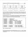
The UPF routine userOl 111is used to realise the creep data input into ANSYS. The data must
be provided by the user as a Set of ASCII files (for each temperature-stress level one Ne). The
structure of a creep data file is demonstrated in the following example:
! ! Temperature K
! ! S t r e s s kPa
!! creep fracture s t r a i n
! ! number o f s t r a i n sets i n t h i s f i l e
6.000003-05
! ! s e t l : epsl d e p s l
! ! s e t 2 : e p s 2 deps2
7.550933-05
! ! s e t 3 : e p s 3 deps3
8.856003-05
! ! s e t 4 : e p s 4 deps4
9.721623-05
1.038663-04
! ! s e t 5 : e p s 5 deps5
Table 1: creep data file example
The creep data nles must be named according to the pattern: basename .C? ? where ?? stands
for the sequent file number (01 dies). To read the creep data files use the following ANSYS
commands /3,41:
....
Extension of the ANSYS@creep and damage simulation capabilities
Page 8
! ! set command name associated with UPF userOl
/ucmd,usr1,1
! ! specify the names and the number of the creep data files
usrl ,filename,nfiles,log-key, intp key
I ! instruct ANSYS to use the User defined creep law
/prep7
tb ,creep ,ma t
tbdata11,1,,,,,100
Table 2: ANSYS input example for using the user defined creep data base
If log key=l, a control output file <jobnam>.crlg is written. If the argument intp-key=V, the
non-linear interpolation scheme is activated (section 3).
For the generation of the creep data files the supporting program CRPGEN is available
(command reference in h e x 2).
3. Calculation of the creep strain increment
To realize the calculation of the creep strain increment according to the non-standard creep law,
the UPF usercrf was modified and linked to the customized ANSYS executable 111. In this
routine the scalar creep strain increment A E = kCr A t is deterrnined from the creep data
(input See section 2) by multi-linear interpolation:
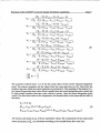
3.1 Linear interpolationi
Assrunulg that the straln rate depends linearly on stress and temperature between two data base
points, the weighting factors in eq, (5) are:
Extension of the ANSYS@creep and damage simulation capabilities
Page 9
The quantities without index E , U ,Tare the a c ~ avalues
l
of the current element inkgration
the
point. The indexed quantities are the values from the creep da& base eq, (3). They
smallest intervals which the actual quantities are enclosed in. The meaning of the Indices is 5:
low bound (largest data base value which is smaller &an the actual integmtion pint ~rilue)md
H: high bound (smallest data base value which 5s greater than fhe actuaZ
an psint
value). The First index refers to fhe ternperature1the second index to tbe stress sind the W d to
the strain.
Extension of the ANSYS@creep and damage simulation capabilities
Page 10
The creep data base eq. (3) has to be provided in such a way that the actual temperature and the
equivalent stress of the elements do not exceed the maximum values of the creep data base. If
the actual temperature or stress values are smaller than the smallest values of eq. (49, the creep
strain increment is Zero for this step.
3.2 Non-linear interpolation
If the temperature steps andlor the stress steps in the creep data base are not sufficiently small,
the creep strain increment might be overestimated, since the strain rate in general depends overproportionally on the stress and on the temperature respectively. That's why a non-linear
calculation of the weighting coefficients is useful.
Assuming that the strain rate depends exponentially on the stress, i.e.
& =
A.0'
the according interpolation between two points is:
the exponent r can be estimated from
Similarly, if it is assumed that the strain rate dependency on the temperature can be described
by
6 = K. e-qIT
(11)
The Parameter q can be estimated fi-om
Of course, the Parameter q can change with the stress level and the accumulated creep strain as
Extension of the ANSYS@' creep and darnage simulation capabilities
Page 11
the Parameter r may be dependent on temperature and strain.
Applying the above equations to the calculation of the weighting coefficients, one obtains:
with the Parameters
It should be noted that in the abave eqiations the index of q, aiways conesponds to &B sesond
index of E„, (stress level) and the index of
(temperatue level).
r, dways corresponds to the fmt index &E „,
Page 12
Extension of the ANSYS@creep and damage simulation capabilities
4. Damage module
4.1 Damage model
The material damage due to significant creep strains is modelled by a damage measure which
is incrementally accurnulated at the end of a load step or substep. This damage includes also the
prompt plastic deformation of the structure. The damage increment is:
zc being the creep fracture strain of the uniaxial creep test at constant stress and
b
with E
Ec
temperature and & the plastic fracture strain (tnie strain) of the tensile test. R, is' a function
which considers the damage behaviour in dependance on the triaxiality of the stress tensor 181:
where 0 , is the hydrostatic stress and (T qv is the von-Mises equivalent stress. Alternatively,
the triaxiality function can be set to 1.
The damage increment is calculated for each element by averaging its nodal equivalent creep
and plastic strains. The accumulated damage is
ldstep
D=
CAD,
If the element damage reaches the value of D=l, the element is killed by setting its death flag
to 1 (refer to the ,,element birth and death" section of 131).
4.2 Calling the damage procedure
The creep damage module is realized in the subroutine -1
and a number of supporting
routines. The invocation of this module is initialized by the User routine USER02. Once this
initialization has been done the creep damage routine is automatically called after each substep
or after each loadstep, depending on the settings with the outres command. This is realized by
the UPFs USOLBEG, USSFTN, and USOLFfN respectively. If ali substeps are written to the
result file (outres,all,all), the damage routine is called after each substep. Otherwise the
damage routine is called after each loadstep (default). If the analysis is a restart analysis, the
previously accumulated damage values are resumed from the binary file <jobnam>.dsav.
Notes:
*
It is not necessary to invoke the usrcal command, the initialization for USOLBEG,
USSFDJ, ULDFiN, USOLFIN and USEROU is done automatically.
Extension of the ANSYS@creep and damage simulation capabilities
Page 13
It is not recornmended to issue outres specifications other than outres,allf/eq, since
element- and DOF-solutions need to be stored on the result file for creep damage
evaluation
To activate the darnage accumulation and the element killing, use the following commands:
! ! set command name associated w i t h UPFs (begin l e v e l )
/ucmd, usr2,2
/ucmd,usr3,3
! ! c a l c u l a t e creep damage
/solu
. .
! ! set the output frequency (optinal)
outres, a l l , f r e q
! ! i n i t i a l i z e the damage procedure
! I the c a l l i n g frequency depends on the outres s e t t i n g s
usr2, ärqcrit
! ! set fracture s t r a i n s
usr3, e p f r key, epbr0, cl tem,c l s i g
-
....
solv
....
Table 3: ANSYS input example for the use of the creep darnage module
The argument dmgcrit of the usr2-command is used to select a damage criterion (dmgcrit-2:
triaxidity according to eq. 17; dmgcrit=l: R, = 1,dmgcrit-0: no damage calculation).
The usr3-command provides an additional possibility to calculate the creep fracture strain or
the plastic fracture strain according to:
+
= epbrO + cltem. T clsig o
epfi- key = 0:
E
epfk- key = 1:
eP1
„-- epbr0+ cltem. T
If the nisr3-command is not entered (or entered with all arguments zero), the current creep
fractu~estrain is calculated from the creep data base values (see creep file example, table 1)by
multi-linear interpolation:
Extension of the ANSYS@creep and damage simulation capabilities
Page 14
For the meaning of the indices see sections 2 and 3. The plastic fracture strain & is calculated
from the last strain-stress point of the MISO-table or of the MKIN table (interpolation between
the temperatures). Refer to the tb, tbpt, tbtemp commands /3,4/.
I
The usr2- and usr3-commands can alsa be used with an ANSYS standard creep law (c6<100),
however, in this case the creep fracture strain must be entered via usr3 since it is otherwise not
available.
After the solv command the scalar ANSYS Parameter ,,dmgmax" is available which represents
the maximum creep damage of all elements at the current loadstep.
Note:
If an element is killed, the stress distribution may promptly and significantly change. So it is
recomrnended to obseme the process of element killing after each load step using the standard
ANSYS commands (esel, "get). If one or more elements are killed during the load step, the time
increment for the next step should be sufficiently small.
1
4.3 Plotting the damage
,
The damage D is calculated for each element whenever the cr-dmg-routine is invoked (section
4.2). To make this quantity available for the postprocessing it is written it to the NMISCrecords of the elements (refer to 151 for the description of the standard non-summable
miscellaneous element output - NPLIIISC). The UPF USEROU was employed to realize the
additional nmisc-output. The damage value is automatically stored on the First place after the
last standard-NMISC output. The graphical output during the postprocessing can easily be
realized with the commands etable, plletab, es01 141. The output frequency to the result file
depends on the settings of the outres command 141. Table 4 shows an ANSYS input example.
>
! ! post-processing
/post1
set,.
..
etable,crdmg,nmisc,26
pletab,crdmg,avg
! ! 26 if elementis plane42
Table 4: ANSYS inputexamPle for plottmg of the creep damage
Note*The aeep
calculated with the stresses and strains of the n-th result set is stored
in the (n+l)-st result set of the result file. This unintended shift is due to the fact that the
USEROU routine is cdled before USSFDN (damage calculation after a substep) and ULDFIN
4
Extension of the ANSYS~creep and damage simulation capabilities
Page 15
(damage calculation after a loadstep). This cannot be influenced by the UPF pragrammer.
However, in the additional file <jobnam>.dmg (see section 5 ) the assignment between the
element results and the calculated damage
- is correct. The command-macro ,,pldmg.macncan be
used as a work around for this problem.
5. Additional files created
5.1 Log-File of creep data base input
To verify the input of the creep data files the log-file cjobnam>.crlg c m be created (jobnam
defaults to ,,filel').This ASCII file contains the base name of creep data files, the number of
temperature levels, the number of Stress levels per temperature, the number of strain rate - strain
pairs for each level and the first twenty of such pairs. The file is written, if the third argument
of the ucri-comrnand is Set to 1: (for example: u s r l ,t e s t c r p ,5,1)
5.2 Log-File of the damage calls
This ASCII file is named <jobnam>.dmg and contains infomation an current load step,
substep, time, number of elements and number of nodes. Moreover, 5or each element the
average temperature, stresses, creep strains, plastic strains and accmulated damage is
recorded. The log-information is appended each time the dmg-routine is called. The file is
newly created in the first loadstep, if the analysis is not a restart.
5.3 Damage backup B e
This binary file is named cjobnam>.dsav and contains the accumulated damage. This file is
necessary if a restart analysis is perfomed. In the case of a restart the crecep data basc must be
input in the Same way as in the first analysis, since the creep data base is not stored in the
db-file (cf. usrl-command), Additionally, the previously accumulated damage must be input
from the dsav-file. This is automatically initialized if a restart analysis is performed.
6 Examples
6.1 Tensile bar
For verification of the creep module a simple model which consists of only one ehrnent was
used (Fig. Al). The creep data base is generated according to equation (1)with the coefficients:
For this ,hyp~theticii~~
matt:nid areference solution can be abta3nIld us
&G
mSYS stzrndmd
Extension of the A N S Y S ~creep and damage simulation capabilities
Page 16
creep equation. So the purpose of this exarnple is
to show that user creep module works correctly
to demonstrate the influence of the interpolation method (cf. section 3)
The load for the model in Fig. A l is a constant streiss of 0 = 200 MPa and the temperature is
1000K. The creep data base is generated for the following temperature and stress levels:
TL= 973.15 K a,= 150MPa o ,= 250 MPa
T, = 1073.15 K a = 150 MPa a = 250 MPa
,
,
(22)
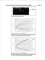
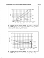
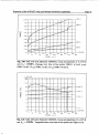
The creep curves are calculated for a time range of 10 s with an integration step width of
0.025s. Figure A2 shows the results for linear interpolation (cf. eq. 6) and Fig. A3 for nonlinear interpolation (cf. eq. 14). With linear interpolation the creep strain is too high (what is
clear in view of eqs. 1 and 21), whereas the results with non-linear interpolation meet exactly
the reference solution.
6.2 Disk with centre hole
The model is shown in Fig. A4. The disk is loaded at its free end by a tensile stress in
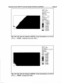
X-direction.Fig. A5 shows the tangential stress of the well known elastic solution exhibiting a
stress maximum of o ,,„ = 30, at the 90' position.
6.2.1 Material behaviour
The material of the disk is assumed to be the French reactor pressure vessel steel 16MND5.
The creep behaviour of this material at high temperatures was investigated within a extensive
experimental program fundedby the European Commission 191. Based on the experimental data
the ANSYS creep data base is generated.
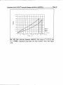
The creep curves are subdivided into three sections (cf. Fig. A6):
I
primary creep range (t C t,)
II
secondary creep range (t, C t C ts)
111
tertiary creep range (t, C t C t,)
The creep curves were generated at different temperature and stress levels according to the
following equations:
Extension of the ANSYS~
creep and damage simulation capabilities
Page 17
For the primary creep stage an equivalent strain hardening representation is:
6 = DIP(T). G dzp(T)
.E
d3~(T)
With
The coefficients of the primary creep stage were taken from the work of IKONEN I91 who
summarized a couple of creep test perfomed in a temperature range of 600-130Q°C.
According
to the experimental data in 191it was assumed that the transition between primary and secondary
creep takes place at a creep strain of & = E, = 0.1 ,and the transition between secondaiy and
tertiary creep at a creep strain of E = Es = 0.2 .The fracture strain is about E = E, = 0.8 .
The times for the creep stages can be calculated by (cf eq. 23):
„
F
1
-
1
To get a smooth transition between the stages of the creep curve the coefficients C„ and CIT
must fulfill the relations:
Table 5 shows the parameters for the creep curves. The coefficients DIP,&3P and d„ are
parameters fitted to the experkents by IKONEN 191, the other coefficients f d o w from Chese
fitted parameters by using the above equations, The coefficients are relakd tu the stress unit
NIPa and the time unit sec.
Extension of the ANSYS@creep and damage simulation capabilities
-0.167
-0.179
-0.3 12
-0.313
eqs. (3,4)
eqs. (3,4)
eqs. ( 3 4
eqs. (3,4)
eq. (3,4)
eqs. (3,4)
eqs. (3,4)
*
Page 18
+
-0.322
-0.304
eqs. (34)
eqs. (34)
TabIe 5: Parameters of the creep curves for the steel16MND5
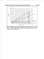
Figure A7 shows the creep strain and the creep strain rate at T=1373 K and o = 10MPa as arm
example.
In some load cases creep and prompt plasticity occur simultaneously. Therefore, the
temperature dependento - E curves aG shown in Figure Ag. A multi-linear isotropic
hardening is assumed and the flow rule of von-Mises is used.
6.2.2 Pure creev at constant temveraiure
At first the development of stresses and damage is studied assuming pure creep (no prompt
plastic deformation) at a constant temperature of 1370 K. The creep deformation leads to a
relatively quick release of the stress concentrationnear the hole. Figures A9 and Al0 show the
tangential stress and the accumulated damage after 1000 s. Figures Al1 and Al2 show the
Same quantities after 9900s. The eiements which were killed in the meantime are not shown. It
is remarkable that in spite of reduced cross section area the maximum stress is still lower than
it was in the beginning of the calculation. This is a consequence of the stress relocation. The
development of the damage and the stress over the time for some locations On the Y-axis is
shown in the Egures Al3 and A14. In Fig. Al4 the effects of stress relocation and of the
element killing can be clealy Seen. Figure Al5 shows the creep strains of the two points (O;rH)
and (O;l.SrH)over the tune. The element at (0;15,) fails at a slightly lower total creep strain
which is a consequence of the higher tnaxiality factor at this location.
Extension of the ANSYS@creep and damage simulation capabilities
Page 19
In this load case creep and plasticity are combined. As before the temperature is constant (1370
K) and the stress load is 0 , = 10MPa .The Figures Al6 and Al7 show the tangential stress
and the accumulated damage after 1000 s. Figures Al8 and Al9 show the Same quantities after
4800s. The development of the damage and the stress over the time for some locations on the
y-axis is shown in the Figures A20 and A21. Figure A22 shows the equivalent creep strain and
the equivalent plastic strain of the two points (O;r,) and (0;lSr,) over the time.
The stress near the hole exhibits a slightly different behaviour compared to the pure creep case
(ref. Fig. A21, red curve). It starts with a lower value since a prompt plastic deformation occurs
and the maximum stress is limited to the initial yield stress. After that the stress is increasing
due to the plastic hardening of the material. After some 800s a stress relocation starts to develop
as a consequence of the increasing creep defonnation.
The Progress of damage looks also somewhat different than in the pure creep case (ref. Fig.
A20). The damage value at t = 0 s is not Zero but up to 0.29. This is the result of the prompt
plastic deformation. The contribution of the plastic strain to the damage leads to a shorter time
at which the f ~ selement
t
fails (4300 s vs. 8400 s in the pure creep case, Fig. A13). The failure
of the first element causes a prompt increase of the damage in the neighbouring elements since
the stress relocation leads to another prompt plastic strain increment. This effect can also be
Seen in the strain curves (Fig. A22). Contrary, in the pure creep case the killing of the first
element only causes a steeper gradient in the damage curves of the neighbouring elements (Fig.
A13).
Comparing the damage (Fig. A20) with the plastic strains and creep strains (Fig. A22) it can be
stated that the relative contribution of the plastic strain to the damage is larger than that of the
creep strain. This is due to the fact that in the case of the 16MNDS steel the plastic fracture
strain is smaller than the creep fi-acture strain (see also eq. 16).
References
ANSYS Programmer's Manual. ANSYS, Inc., 1998
ANSYS User's Manual - Theory (Rev. 5.5). ANSYS, Inc., 1998
ANSYS User's Manual - Analysis guide (Rev. 5.5). ANSYS, Inc., 1998
ANSYS User's Manual - Command reference (Rev. 5.5). M Y S , Inc., 1998
ANSYS User's Manual - Elements manual (Rev, 5.5). ANSYS, Inc., 1998
Becker, A.A.: Background to Material Non-Linear Benchmarks. NAFEMS-report
R0049 (International Association for the Engineering Analysis Comunity)
Azodi, D., P. Eisert, U. Jendrich, W.M. Kuntze: GRS-Report GRS-A-2264
Lemaitre, J.: A Course on Damage Mechanics. ISBN 3-540-60980-6, 2nd edition
Springer-Verlag Berlin, Heidelberg, New York, 1996
Ikonen, K., 1999, "Creep Model Fitting Derived from REVISA Creep, Tensfie and
Relaxation Measurements", Techical Report MQSES-4/99, VlT-Energy, Espoo,
FUlland.
Extension of the ANSYS@creep and damage sirnulation capabilities
Appendix 1: Figures
Page 20
Extension of the ANSYS' creep md damage simulation capabilities
I
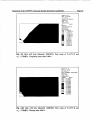
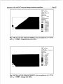
Fig. Al: Model of the tensile bar
I
t i m e
C s )
~IG=~~OMPA,T=~OOOK,DELTA-SIG=~~O,DELTA-T=~O~
Fig. A2: Tensile bar, creep curves (axial strain and lateral strain)
vs. time, linear interpolation and reference solution.
t i m e
Cs)
SIG=SOOMPA,T=~OOOK,DELTA-SIG=ICIO,DELTA-T=IW
Fig. A3: Tensile bar, creep curves (axial strain and lateral strain)
&time, non-linear interp&tion and reference solution
Page 21
Extension of the ANSYS@creep and damage simulation capabilities
Page 22
Fig. A4: Model of the rectangular disk with a centre hole; uniform stress at x=a
(red); symmetry conditions at x=O and y=O (blue)
ANSYS 5.6
MAY 22 2000
09:58:14
NODAL SOLUTION
STEP=l
SUB =1
Hg. A5: Tangential stress (elastic solution)
Extension of the ANSYS@creep and damage simulation capabilities
Page 23
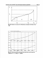
Fig. A6: Scheme of a creep curve with primary, secondary and tertiary creep
Stage
.......t .................
1DDE.io.ltime
........--............ ..-.................
;
1.50E+04
Z.OOieW4
2.5DEiU4
3.W.io.l-
Fig. A7: Creep curves (creep strain and creep strain rate over the h e ) for
16MNl35 at T = 1373% o = 10MPa.
MISO Table For Material
1
m s Y S 5.6
MAY 25 2000
18:32:49
Table Data
{X
lO+*61
EPS
Fig. Ag: Stress-strain-cnwes of 16MND5 for the temperaturerange from 300K to 1475 K
(tnre stress and strain) based on /9/.
Extension of the ANSYS@creep and dafnage simulation capabilities
Page 25
ANSYS 5.6
MAY 23 2000
ll:36r19
NODAL SOLUTION
STEP=ll
SUB =I37
TIME=1000
SY
WJG)
RSYS=l
PowerGraphics
EFACET=l
AVRES=Mat
DMX =.026037
S m =- .102E+08
SMX =.1983+08
Fig. Ag: Disk with hole (Material 16MND5). Pure creep at T-1373 K and
o = 1 0 W a .Tangential stress &er 1000 s.
,
ANSYS 5.6
MAY 23 2000
11:37:17
AVG ELEMENT SOLUTlON
STEP=11
SUB =P37
TIME=POOO
CRDMG
{AVG)
DMX =,026037
SMN =,004353
SMX =-P67568
,004353
Extension of the ANsYS@ creep and darnage simulation capabilities
Page 26
ANSYS 5 - 6
MAY 23 2000
12:16:59
NODAL SOLUTION
sTE P=10 3
SUB =439
~1~~=9900
SY
(AVG)
RSYS=l
powerGraphics
EFACET=l
AVRE S=Mat
DMX =.I07927
sMN =-.126E+08
SMX =.182E+08
Fig. All: Disk with hole (Material 16MND5). Pure creep at T-1373 K and
G, = 10MPa. Tangential Stress after 99OQ s.
ANSYS 5.6
MAY 23 2000
12:17:46
AVG ELEMENT SOLUTION
STEP=103
SUB =439
TIME=9900
(AVG)
CRDMG
DMX =.X07927
SMN =.OS2717
SMX =.962179
Extension of the M Y S @ creep
'
arid damage simulation capabilities
Page 27
I?m-3
DPIG- C
< %
2.4
4
5.6
7.2
8.8
30*X3>
10.4
T I M E Cs)
Fig. A13: Disk with hole (Material 16-5).
mire creep at T-1373 K and
o = 10MPa. Damage over time at four points: DMG-1 at (X+ y-r,), DMG-2
at (0; 1.5 r,), DMG-3 at (0; 2.5 rH),DMG-4 at (0; b).
,
Hg. Al& Disk ~4thhole (Material 16-5)Pure meep at T4373 K md
cr = I(bWa. Tangentil sbms over time at four points (see F i p A13)
,
Page 28
Extension of the ANSYS@'creep and darnage Simulation capabilities
-00
.90
.80
.70
.60
.50
.40
.30
E PPL-2
EPEL-1
EPCR-2
E PCR- 1
-20
.10
X
0
2.4
4
5.6
7.2
8.8
lO*$3)
0.4
TIME C SI
Hg. AIS: Disk with hole (Material 16MND5). Pure creep at T-1373 K and
0 , = 10MPa. Equivalent creep strain over time at points 1 and 2 (See Figure
A13)
Extension of the ANSYS@creep and damage simulation capabilities
Page 29
ANSYS 5.6
JUL 6
. 2000
12:52:44
NODAL SOLUTION
STEP=11
SUB =I34
TIME=1000
(AVG)
SY
RSYS=l
-
-
P
PowerGraphics
EFACET=l
AVRE S=Mat
DMX =.027558
SMN =-.203E708
SMX =.200E+08
- .lO3E+O8
- .695E+O7
-.359E+07
-221048
-31534-07
.651E307
-9883307
0 .l3SE+O8
0 -166E-J-08
-200E4-08
rn
m
rn
and o = 10MPa. Tangential stress after 1000 s.
ANSYS 5 - 6
JUL 6 2000
12:53:19
AVG ELEMENT SOLUTION
STEP=11
SUB =I34
TIME=1000
DMO
(AVG)
DMX =,027558
SMN =.004256
SMci =.656388
OOi%256
1 O76XI.5
-149174
-221633
11 -294092
-366553
43SOlX
-51147
,583929
-656383
.
m
.
-
Fig.
hole (Material
and o = lioma.Damage afkr 100-0s,
,
Extension of ihe ANSYS@creep md darnage simulation capabilities
Page 30
ANSYS 5.6
JUL 6 2000
13:05:52
NODAL SOLUTION
STEP=53
SUB =I45
TIME=4800
SY
WJG)
RSYS=l
PowerGraphics
EFACET=l
AVRE S=Mat
DMX =.063181
SMN =-.108E+08
SMX =.184E+08
Fig. AIS: Disk with hole (Material 16MND5). Creep and plasticity at T-1373 K
and o = 10MPa. Tangential stress &er 4800 s.
,
ANSYS 5.6
JUL 6 2000
13:06:37
AVG ELEMENT SOLUTION
STEP=53
SUB =I45
TIME=4800
DMG
WJG)
DMX =.063181
SMN =.013981
SMX =I-005
Pig. A19: Disk with hole (Material 16MND5). Creep and plasticity at T=1373 K
and 0 , = 10Pc/lPi1.Damage &er 4800s.
Extension of the ANSYS@'creep and damage simulation capabilities
Page 31
Fig. A20: Disk with hole (Material 16MND5). Creep and plasticity at T=1373 K
and a, = 10MPa. Darnage over time at four points: DMG-1 at (x=O; y=r,),
DMG-2 at (0; 1.5 r,), DMG-3 at (0; 2.5 r,), DMG-4 at (0; b).
and
(r
= 10MPa. Tangential str;ess w e r b e at four points (see Pigure Al31
Extension of the ANSYS@creep and damage simulation capabilities
Page 32
Fig. A22: Disk with hole (Material 16MND5). Creep and plasticity at T=1373 K
and o = 10MPa .Equivalent creep strain and equivalent plastic strain over time
at points 1 and 2 (see Figure A13)
,
Extension of the ANSYS@creep and darnage simulation capabilities
Appendix 2: CRPGEN command reference
Page 33
Page 34
CRPGEN for Win NW9x (Rev 1.4) - Cornrnand Reference
CRPGEN for WIN NT I 9x (Revision 1.4)
Command Reference
clear
Delete all preceding settings of the crdat, time, epmax, sigma, ternp comrnands.
Set the creep Parameters (C,-C+,-C,) and select creep law (C,). SZOCrefers to the fxst
creep pararneter to be input (e.g. crdat,#,cl , ~ 2 , reads
~ 3 the constants C„ C, and C,).
If C, = 0 use strain hardening model according to:
&
= C*.oC2. & C 3 .
If C,
(C, is unused)
= 1 use time hardening model according to:
-
-
(C, is unused)
If C,
= 2 use time hardening model according to:
(C, is unused)
Convert a creep function to another stress unit system (e.g. from Pa to MPa). This command
can be used to change existing creep data files to use them in different engineering unit
Systems. The stress level in a creep data file is changed according to:
o „ = sigfac.o
sigoff The command should only be used in connection with read
and write.
,
+
.
Example:
read,filel .c01
cnvsig,l.Oe+06
wriL,file2.cOl
Define the maximum strain up to which the creep curve (E) is to be generated. Command
is required for C, 0 (see crdat).
-
CRPGEN for Win NT19x (Rev 1.4) - Cornrnand Reference
Page 35
exit
Terminate the program. The data base is not automatically saved. Use the write command.
plot,pW
Plot creep curves. If plkey = 0,plot E (t) and E (t) ,if plkey = 1 plot E (E)
.
prdat
Print creep parameters to standard output.
readJizame
Read a creep data file. fname is the ASCII file containing a creep curve
E = (E)lo=const;T=anst
rsolve
Continue the solurion after the change of creep parameters. This command can be used to
generate creep curves which are govemed by different creep equations (e.g. primary,
secondary and tentiary creep stage). A solve command must have been entered before the First
rsolve command. An additional time or epmax command is also required, where the
endtime or epmax argurnent must be greater than that of the previous solve or rsolve process.
Stress and temperature must not be changed after the solve command.
Exam~le:
sigma,100
temp,800
crdat,l,l.Oe-16,2.2,-0.14,9860,0,1
time,3000
steps,200
solve
crdat,l,3.Oe-15,2.2,0!01,9860,0,1
time,5600
steps,l50
rsolve
write,crpdat.cOl
Defme the Stress level for the creep curve.
CRPGEN for Win NTI9x (Rev 1.4) - Command Reference
Page 36
Start generation of creep data. Command requires creep parameters to be input (see crdat,
time, epmax, steps).
steps,nstep
Defm the nurnber of time 1 strain steps; nstep pairs [E;
E] are to be generated.
temp,temp
Define the temperature level for the creep curve to be generated.
Set maximum time for creep data generation to endtime. This command is required for C,
(see crdat-command) and for plotting time-dependent creep curves (see plot,O)
writeiame
Wnte generated creep data to the ASCII filefname.
=
1
CRPGEN for Win NTI9x (Rev 1.4) - Comrnand Reference
Page 37
General Shell Commands (Macro-Langua~e)
delvar
Clear all defmed variables. See also: Definition of variables, *stat
Execute a do-loop within a command fie (see fmp). The command is not possible fiom
standard input. The loop variables dostart,dostop,dostep can be numbers, variables or
expressions (dostart C= dostop; dostep > 0). The loop must be closed by *enddo in the Same
command file where it was opened. The loop body must not refer to another cornmaud file.
Up to 10 do-loops can recursively be opened at the Same time.
Switch odoff command echo to standard output
Terminate the input stream from the current input file and redirect it to the prior unit.
help
Open help file (Acrobat Reader required).
*if,exprl,op,exprZ,then
cornmand-block
[*elseif,exprl,op,exprZ,then]
[command-block]
Branching within a command file (not possible fiom standard input). aprI aad expr2 are
numerical values, variables or expressions; op={eq, ne, lt, gt, le, ge). ?'he syntax is sunilar to
ihe FORTRAN programming language, but *endif and then are required, h u f s i v e ifstatements are possible.
Page 38
CRPGEN for Win NT/9x (Rev 1.4) - Command Reference
Directs input stream to file fname. Recursive switches are possible.
If files with extention ,,.macl'(macros) are existing in the current working directory, these
macros files can be input by simply typing the basename of the macro file (e.g. type ,,macOl"
to input the comrnand file ,,macOl .mact').
Switch program printouts fiom standard output to file jhame. If fname is not input, switch
back to standard output.
Print all defined variables. See also: Definition of variables, delvar
Definition of variables
Variables can be defmed by
vur=value
where value can be a number, a name of a variable, a numerical expression or a character
string. The name of the variable var must begin with a letter and can consist of 8 characters.
Expressions can be assembled fiom numbers and numerical variables. Valid operators are:
left (opening) bracket: (
right (closing) bracket: )
plus (addition): +
minus (subtraction):
multiplcation: *
division: /
power operation:
-
**
The defined variables are global ones. The character equivalents of variable values can be
used in command strings by: stri%varname%str2 (%vamame% is replaced by its character
value). For example the following conunands are equivalent:
varl ='xyz'
read,file%varl %
read ,filexyz
Floating point variables are truncated to integer. If for example a=3.25E+01, then the result
of %a% is .321t.