Download Topica3 user manual, version 0.3

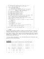
Topica3 user manual, version 0.3
Daniele Milanesio, [email protected], +390115644077
HTU
UTH
Gid
Gid is the graphic tool adopted to draw the antenna. First, copy the “ANTENNA.gid”
folder inside the gid “problem types” folder; second, before starting the design of the
antenna, select the material on the “Data” window and click over “Problem type”
choosing “ANTENNA”, in order to allow the use of the set of materials on which the
code is based.
If you want to compute electric fields somewhere in the antenna region, you need to
include in the antenna drawing dedicated surfaces that are used only for this task and on
which the magnitude of the electric field will be determined; in fact, these “electric field
surfaces” are neglected in the analysis and determination of antenna parameters.
Once the antenna drawing is completed, before doing the mesh, assign to every surface
the correspondent material: “Antenna” for the antenna structure, “Aperture” for its
aperture (in the case of presence of plasma), and “Electric Field” for dedicated surfaces
(in case you require the electric field visualization).
Then, according to the feeding, you can perform two different operations: if the coaxial
feeding is included, assign to every surface belonging to a coaxial line the correspondent
material (from “Port1” to “Port16”) and then mesh the structure. In case of voltage gap,
once all the surfaces are described (“Antenna”, “Aperture” or “Electric Field” material),
mesh the structure. Then, you need to directly identify the triangles that belong to every
port: color with the correspondent port material (from “Port1” to “Port16”) every T+
triangle of the RWG function and with “Ground” material every T- triangle. If the T+
triangle belongs to a junction, you don’t have to care about the T- assignment, this will be
automatically done by Topica3 code.
We suggest, in all cases, to use the layer window, in order to visualize only some
surfaces, above all if the antenna is quite complex (it is really difficult to find a triangle in
a 3D mesh if the entire antenna is visualized!).
When the antenna is completed and the feeding has been identified, you can export the
mesh in a file (i.e.: structure.txt) that can be read by Topica3 code.
U
Brief description of modules
U
• triangoli.inp
It contains all the input parameters that must be set to properly run the complete Topica3
code; all the parameters are described inside the file but they will be analyzed in the
following lines. This is the content of “triangoli.inp” file:
Dloop
3
.false.
1 2
structure name → should be coherent with the mesh file from
gid.
integration threshold → it represent the distance used to
distinguish close from distant triangles. After several
simulations 3 appeared to be the optimum value.
ground plane → when it is set to TRUE an infinite ground
plane is positioned in z=0.
distant triangles → it express the number of sampling
points adopted in the external and internal integral in
5 4
2 3
4 4
0.25
0.2E+9
1.0E+9
9
.false.
.false.
.false.
.false.
2
1 0 50
0.02 0.005
0.0595
0
0
1 0 50
0.02 0.005
-0.0595
0
0
case of distant triangles. Topica3 decides if two triangles
are distant or close according to the previous parameter
(0.25) and, consequently, to the working frequency.
Different formulas are implemented according to the next
scheme:
1 → degree 2, 3 points
2 → degree 2, 9 points
3 → degree 5, 7 points
4 → degree 7, 16 points
5 → degree 1, 1 point
close triangles
coincident triangles
coincident/close triangles
this parameter is used to evaluate if a triangle of the
mesh is too large; when this happens Topica3 produces some
warnings on the output file but matrices are nevertheless
computed.
starting frequency
ending frequency
frequency points
efie → this parameter is set to TRUE in case of EFIE set of
equations (antenna in vacuum) and to FALSE when the ibryd
formulation is adopted (antenna toward plasma).
coax → this parameter is set to TRUE when coaxial feeding
is adopted while has to be FALSE in case of voltage gap
spectral contribution → this parameter is set to FALSE only
in case of plane aperture toward vacuum (the only case in
which the module “topstc40” has not to run)
currents → this parameter is set to TRUE when we need to
save currents on RWG functions (both magnetic and electric)
and when we need to compute electric fields
number of ports (≥1)
real and imaginary part of voltage and reference impedance
at first port (always present)
outer and inner radius of first coax cable (all data
referring to coax feeding like dimensions or coordinates
has to be removed when coax is set to FALSE, only voltage
values has to be preserved)
first coax center (x coordinate)
first coax center (y coordinate)
first coax center (z coordinate)
voltage and reference impedance at second port
radius of second coax cable
second coax center (x coordinate)
second coax center (y coordinate)
second coax center (z coordinate)
In case of more ports, all data related to every port has to be added with the same format,
according to feeding (voltage gap or coaxial line).
The file ‘triangoli.inp’ is an input file for ReaderM2, Asterione, Zem15 and Post4.
• ReaderM2
It is the first program that has to be run after the creation of the antenna; it is used to
transform the Gid output geometry file (i.e.: structure.txt) into a complete mesh file (i.e.:
structure.mix.msh) that will be the input for all the following modules. It also produces a
file (PtX.mom) for every port assigned.
• Asterione
It computes all self terms (electric-electric and magnetic-magnetic contribution); it
always saves a “Ztem11_fX.txt” file for every frequency point and, when EFIE parameter
is set to FALSE (antenna toward plasma), a “Ztem22_fX.txt” file. These two files store
the electric and magnetic self interaction between RWG functions. In case of electric
fields computation, it also saves the contribution to the total electric field due to the
electric currents on conductors (stored in “Z11field_fX.txt”).
• Zem15
It computes electric-magnetic interactions, port subdivision and some matrices for
coaxial feeding. When EFIE is set to TRUE it only determines the port files, both in case
of voltage gap and coaxial feeding; when EFIE is set to FALSE, it also saves a
“Ztem12_fX.txt” file for every frequency point. If coaxial feeding is set to TRUE, it also
saves an “Ep_pX_fX.txt” term for every port at every working frequency that will be
used by post-processing module. In all cases a “freq.txt” file is generated to establish
correspondences between every matrix and its working frequency (i.e.: _f1 → 80 MHz).
In case of electric fields evaluation, this module produce the contribution due to magnetic
currents (stored in “Z12field_fX.txt”) and due to the primary currents (stored in
“Epfield_pX_fX.txt”), when the coaxial cable feeding is adopted.
• Topstc40
This module computes the spectral contribution to the interaction matrix. It has to be
launched in all cases (obviously when EFIE is set to FALSE), except when we deal with
antennas with plane aperture toward vacuum. The necessary input files are the mesh of
the antenna generated by “ReaderM2” module and the data file “df.std”, that contains
relevant geometrical and physical parameters that are to be set according to the antenna
and plasma models.
To carry out a complete simulation using a hot plasma model, “Topstc40” has to be used
twice: first of all in order to obtain the samples of the spectral variable pairs (kt, phi),
which are fed to “FELICE” code; second, once “FELICE” has generated the
“BrambXX.mom” output files, “Topstc40” need be run again to determine the plasma
interaction matrix contribution, which is eventually saved to files named “Gp_fX.std”,
wherein X is a progressive integer number denoting a frequency point.
A complete and exhaustive description of the “df.std” input file is contained at the bottom
of the same file and reported here:
+--------------------------------------------------------------+
| Input data description:
|
| * geoname: name of file containing the structure
|
|
description (*.mix.msh)
|
| * dcellamax: maximum dimension of cell edge
|
|
(normalized to lambda0min)
|
| * nt2: number of kt samples in [0,2k0]
|
| * nfimin: minimum number of phi samples in [0,2pi]
|
| * tol: tolerance for integrals in [2*k0,kt_max]
|
| * s: intersection of aperture with x-axis [m]
|
| * b: intersection of plasma with x-axis [m] (b>=s)
|
| * A,B,R: major and minor torus section axes
|
|
and torus radius [m]
|
| * mapping procedure flag:
|
|
1: stretching is performed
|
|
0: no stretching is applied and A,B,R are ignored
|
| * fsam,fin,ffin: number of samples, start and stop
|
|
frequency [Hz] respectively
|
| * ne: edge electron density [1/m^3]
|
| * nD: edge deuterium density [1/m^3]
|
| * nT: edge tritium density [1/m^3]
|
| * nH: edge hydrogen density [1/m^3]
|
| * nHe: edge helium density [1/m^3]
|
| * Bo,alpha: static magnetic field [T] and tilt angle [deg] |
|
of Bo with respect to toroidal positive direction
|
| * kthot: radius [1/m] of hot plasma spectrum
|
|
(it is actually relevant only if hot plasma is used)
|
| * dmax: max distance between cells [m]
|
| * plasma flag:
|
|
-1: only compute and save kt and phi for input to FELICE |
|
0: vacuum
|
|
1: with plasma
|
| * FELICE flag
|
|
0: cold plasma
|
|
1: hot plasma after FELICE
|
| * output flag
|
|
0: compute magnetic-magnetic interaction matrix Gp
|
|
1: compute power and field spectra
|
+--------------------------------------------------------------+
| $Version 4.0 for use with TOPSTC40.FOR
|
+--------------------------------------------------------------+
• Post4
Post processing program that builds the complete interaction matrix and evaluates the
admittance matrix. The input files are all the matrices saved by “Zem15”, “Asterione”
and “Topstc40” modules. “Post4” saves on a file the admittance matrix and, if currents
parameter (see “triangoli.inp”) is TRUE, also electric (and magnetic when EFIE is
FALSE) currents and electric fields.
!!!!) Every module also produces a “test” file that can be used to check some extra
parameters involved in the simulation.
On Mesh file
Here there is a typical example of mesh file after the “ReaderM2” module:
U
1
1
1
2
1
3
…….
1
3857
1
3858
2
1
2
2
2
3
…….
2
3631
-.427913E+00
-.423045E+00
-.367285E+00
.400000E+00
.377412E+00
.400000E+00
.397018E+00 -.400000E+00
.394543E+00 -.400000E+00
2
2240
2116
2125
1
2
2240
2125
2298
1
2
2856
2985
3184
1
2
707
627
770
99
1
1
1
.341234E-01
.899300E-01
.266793E-01
0
0
0
0
0
0
1
1
0
0
0
.344798E+00
.369684E+00
0
0
0
0
0
2
…….
2
2
…….
2
2
2
2
2
2
…….
2
2
3
3
3
…….
3
3
3632
2
1971
5003
5004
2
2
1138
978
6007
6008
6009
6010
6011
6012
2
2
2
2
2
2
3344
3209
1123
1148
1016
1150
6169
6170
1
2
3
2
2
6604
6605
4907
4907
1989
978
902
3209
3153
1148
1008
1150
1127
2623
2897
2893
2897
1
26
1
1
2
1
1
850
1
4908
5013
2
2
2145
1076
1076
3206
3148
1150
1150
1008
1123
2893
3257
0
0
0
0
0
0
0
0
0
0
99
2
2
21
21
1
1
23
23
1
1
0
0
0
0
0
0
0
0
0
0
0
0
0
0
0
0
The first column represents the element type (1→vertex, 2→triangle, 3→RWG function),
while the second one is used to number all the elements (obviously starting from 1 to the
total number of vertices, triangles and functions).
The third, fourth and sixth columns of the vertices block stand for the Cartesian
coordinates of every vertex (in order x, y, z).
Once all vertices are stored, the triangle data block starts; in this case, columns number 3,
4 and 5 contain the index of the three vertices of the triangle (i.e.: triangle 1 is made up of
vertices 2240, 2116 and 2125). Column 7 is adopted to identify the role of every triangle:
1 means that the triangle has electric currents, 2 means that the triangle has both electric
and magnetic currents, 21÷36 are used to fix T+ triangles of every port and 99
corresponds to all T- triangles belonging to a port. For further details on materials
assignment, please refer to the first section.
Finally, the last part shows all data referred to RWG functions. Column 3 and 4 refers to
the index of triangle T+ and T- of the correspondent function (i.e.: RWG 1 is made up of
triangle T+ 1 and T- 26), while column 5 identifies again the material of an RWG. In this
case 1 is used for every RWG with electric currents (also for RWG belonging to ports)
while 2 stands for RWG on the aperture of the cavity, where both electric and magnetic
currents flow.
All other fields contain parameters that are not taken into account by Topica3 code.