Download Truck-Rail Intermodal Toolkit: User Manual (0

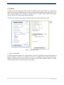
Truck-Rail Intermodal
Toolkit:
User Manual
0-6692-P2
http://library.ctr.utexas.edu/ctr-publications/0-6692-P2.pdf
0-6692-P2
Truck-Rail Intermodal Toolkit: User Manual
Dan P. K. Seedah
Travis D. Owens
Robert Harrison
TxDOT Project 0-6692: Truck-Rail Intermodal Flows: A Corridor Toolkit
JUNE 2013; PUBLISHED SEPTEMBER 2014
Performing Organization:
Center for Transportation Research
The University of Texas at Austin
1616 Guadalupe, Suite 4.202
Austin, Texas 78701
Sponsoring Organization:
Texas Department of Transportation
Research and Technology Implementation Office
P.O. Box 5080
Austin, Texas 78763-5080
Performed in cooperation with the Texas Department of Transportation and the Federal Highway Administration.
Table of Contents
Introduction and Installation ........................................................................................................... 1
1.
System Requirements ....................................................................................................... 1
2.
Installation ........................................................................................................................ 1
CT-Rail ........................................................................................................................................... 3
1.
Upload Track Data ........................................................................................................... 3
2.
Select Equipment and Cargo ............................................................................................ 5
3.
Run Pre-Process ............................................................................................................... 6
4.
Select Locomotives and Specify Horsepower per Trailing Ton Ratio............................. 7
5.
Specify Travel Time, Rail Capacity, and Delay Calculations.......................................... 8
6.
Fill in the Cost Modules ................................................................................................... 8
7.
View the Cost Summary Sheet....................................................................................... 12
8.
Guide to Rail Capacity and Delay Estimation ............................................................... 13
Rail Line Comparison ................................................................................................................... 17
1.
Input Operating Parameters ............................................................................................ 17
2.
Upload Track Data ......................................................................................................... 17
3.
Select Equipment and Locomotives ............................................................................... 17
4.
View Model Output ........................................................................................................ 18
CT-Vcost Lite ............................................................................................................................... 20
1.
Input Vehicle Information .............................................................................................. 21
2.
Specify Route Information ............................................................................................. 22
3.
Run Simulation............................................................................................................... 22
4.
View CT-Vcost Model Output ....................................................................................... 22
Highway Improvement ................................................................................................................. 24
Support .......................................................................................................................................... 28
List of Figures
Figure 1: CT-TRIT.xlsx file ............................................................................................................ 1
Figure 2: Home Screen ................................................................................................................... 2
Figure 3: CT-Rail Screen ................................................................................................................ 3
Figure 4: CT-Rail Track File Format .............................................................................................. 4
Figure 5: Sample Track Data Files ................................................................................................. 4
Figure 6: “Upload Track Data” Button, “Show Graph” Button, and Start/End Fields. .................. 4
Figure 7: Sample Track Speed and Elevation Profile ..................................................................... 5
Figure 8: Equipment Selection and Cargo ...................................................................................... 6
Figure 9: Rolling Stock Statistics ................................................................................................... 6
Figure 10: Locomotive and HPTT Ratio Selection ........................................................................ 7
Figure 11: Travel Time, Rail Capacity, and Delay Calculations .................................................... 8
Figure 12: Overview of CT-Rail Cost Modules ............................................................................. 9
Figure 13: Labor Cost Module ........................................................................................................ 9
Figure 14: Fuel Cost Module ........................................................................................................ 10
Figure 15: Loading and Unloading Cost Module ......................................................................... 10
Figure 16: Emissions Module ....................................................................................................... 11
Figure 17: Maintenance Costs Module ......................................................................................... 11
Figure 18: Capital Costs Module .................................................................................................. 12
Figure 19: Cost Summary Sheet ................................................................................................... 12
Figure 20: Rail Capacity and Delay Module ................................................................................ 13
Figure 21: Delay Volume Curve ................................................................................................... 16
Figure 22: Rail Line Comparison Model ...................................................................................... 18
Figure 23: Rail Line Comparison Output ..................................................................................... 19
Figure 24: CT-Vcost in TRIT ....................................................................................................... 20
Figure 25: Route Information Sheet ............................................................................................. 22
Figure 26: “Run CT-Vcost Lite” button ....................................................................................... 22
Figure 27: CT-Vcost Operating Cost Output by Time Step ......................................................... 23
Figure 28: Highway Improvement Interface................................................................................. 25
Figure 29: Sample Input Data Showing Roadway Geometry (HCM, 2010) ................................ 26
Figure 30: Sample Traffic Demand Data in 15-Minute Increments ............................................. 26
Figure 31: Highway Improvement Model Output ........................................................................ 27
Introduction and Installation
The truck-rail intermodal toolkit (TRIT) was developed to help planners equally compare truck
and rail freight movements for specific corridors and to give insight into some of the variables
associated with each mode. The rail component of the model (CT-Rail) is designed to help
planners and policy makers understand rail corridor operations and examine the opportunities
and challenges for modal shifts from truck to rail. CT-Rail uses a mechanistic approach that
adequately captures the effects of cargo weight, running speeds, network capacity, and route
characteristics—key factors that are essential in any logistical analysis. The truck component of
TRIT, CT-Vcost, developed from an earlier TxDOT study, allows planners to simulate truck
movements over a specified corridor given factors such as truck speed, equipment depreciation,
financing, insurance, maintenance costs, fuel cost, driver costs, road use fees (e.g., tolls), and
other fixed costs—factors that influence truck operating costs and delivery time. Comparative
variables used in both models include roadway and track characteristics (elevations and grades),
travel speeds, changes in fuel prices, maintenance costs, labor costs, and tonnage. The truck
corridor model also accounts for toll rates and vehicle insurance costs; drayage costs are included
only in the rail corridor model. Outputs from both models include fuel consumption and cost,
travel time, and payload cost per ton-mile.
The final report of TxDOT study 0-6692, “Truck-Rail Intermodal Flows: A Corridor Toolkit,”
will provide a detailed explanation of the methodologies discussed in this user manual.
Following its publication, that report (0-6692-1) will be posted online courtesy of the CTR
library.
1. System Requirements
Microsoft Excel 2007 or 2010
2. Installation
1. Insert the provided CD into your CD-ROM drive.
2. Select your CD drive in “My Computer” (XP) or “Computer” (Vista/7).
3. Double-click on TRIT.exe to extract files to preferred location.
4. Locate the Microsoft Excel File CT-TRIT.xlsx—this is the application (see Figure 1 for
the file icon).
Figure 1: CT-TRIT.xlsx file
5. Click on that file to reach the home screen, shown in Figure 2.
1|Page
Figure 2: Home Screen
2|Page
CT-Rail
CT-Rail is the rail component of the toolkit. It enables planners and analysts to examine how
operational changes, freight demand, and route characteristics influence operating costs, travel
time, fuel consumption, and emissions. Clicking on the “CT-Rail” button found on the home
screen will take you to the screen shown in Figure 3.
To return to the home screen, simply click the Home icon on the right of the screen.
Figure 3: CT-Rail Screen
1. Upload Track Data
CT-Rail requires track data to be in the form of a CSV file, formatted with the fields shown in
Figure 4. Distance (in miles), Y-coordinate (Ycoord), X-coordinate (Xcoord), Elevation (in feet),
Speed (in miles per hour), and Curvature (in degrees) are the fields available; however, Ycoord,
Xcoord, and Curvature are not required to run the model.
3|Page
Distance Ycoord
0
0.02799
0.22803
0.52696
0.90597
0.99702
1.04999
1.26503
1.45391
1.65492
1.83097
2.021
2.28796
2.51607
2.89595
Xcoord
0
0
0
0
0
0
0
0
0
0
0
0
0
0
0
0
0
0
0
0
0
0
0
0
0
0
0
0
0
0
Elevation Speed
602.7
601.5
592.6
597.2
605.2
603.8
605.5
612.3
619.2
628.7
634
640
652.6
662.2
679.6
40
40
40
40
40
40
40
40
40
40
40
40
40
40
40
Curvature
0
0
0
0
0
0
0
0
0
0
0
0
0
0
0
Figure 4: CT-Rail Track File Format
Four sample track data files are supplied in the folder “Sample Track Data,” as Figure 5 shows.
Figure 5: Sample Track Data Files
Clicking on the “Upload Track Data” button will open a window from which you can select the
desired track data file. After the data uploads, the “Show Graph” icon will appear to the right of
the “Upload Track Data” button (Figure 6); clicking the graph icon will display the speed and
elevation profile of the track as shown in Figure 7. If you’d like to work with only a section of
the uploaded track data file, specify the starting and ending mile posts using the “Start” and
“End” text fields (labeled with the phrase “Specify Starting and Ending Mile Post for Analysis”).
Figure 6: “Upload Track Data” Button, “Show Graph” Button, and Start/End Fields.
4|Page
Figure 7: Sample Track Speed and Elevation Profile
2. Select Equipment and Cargo
After the desired route data file is uploaded, select equipment type and cargo weight using the
controls shown in Figure 8. You can choose from these options:
•
Type of Container:
– 20 ft. Dry, 20 ft. Reefer, 40 ft. Dry, 45 ft. H. Cube, 40 ft. Reefer, No containers
•
Number of Containers (which is the also equivalent to number of cars for non-container
movements)
•
Weight of Cargo per Container (in tons)
•
Double Stacked: Check this option box if containers are double stacked; otherwise
uncheck. Checking this box will increase the cargo weight per rail car and influence the
total number of cars, train length, and rolling stock weight, as shown in Figure 9.
•
Utilization ratio (in percentages), i.e., percentage of containers that are full
•
Car Type: This dropdown menu becomes available only when the container type chosen
is “No Container,” presenting the following options:
– Auto Transporters, Boxcars, Center Partition Railcars, Container Carriers (5-unit),
Gondolas, High Cube Box Cars, Hoppers, Intermodal Flatcars, Other Flatcars,
Tankers
5|Page
Figure 8: Equipment Selection and Cargo
Figure 9: Rolling Stock Statistics
3. Run Pre-Process
The Pre-Process module performs calculations prior to simulating train movement along the
route to determine the necessary constraints and number of locomotives required to move rail
cars. The calculations involve determining the maximum (governing or ruling) grade, the
maximum resistance encountered, and the minimum horsepower required for the train to traverse
the track.
6|Page
Average engine efficiency for the locomotives can also be specified at this point (see Figure 9).
The most important parameter is the Solution Step input. Ruling grade, maximum resistance, and
required horsepower are calculated at a specified incremental distance (the “solution step”) along
the uploaded track. Increasing or decreasing this value influences the calculating time of the
model and slightly influences the model’s accuracy. For example, total fuel consumed may vary
from 1% to 5% depending on whether the solution step is 1 mile per iteration or 0.1 mile per
iteration. The recommended solution step for most Pre-Process simulation runs is 0.1 miles.
Click on “Begin Pre-Process” to complete Pre-Process module calculations.
4. Select Locomotives and Specify Horsepower per Trailing Ton Ratio
The total number of locomotives required is dependent on the horsepower of each locomotive
and the desired horsepower per trailing ton (HPTT) ratio. The HPTT ratio is determined by the
railroads, and varies by route and service type. It dictates the desired maximum speed of the
train. The typical HPTT ratios used by Class I railroads vary between 2.5 to 3.5 for intermodal
movements, but decrease for other heavier cargo such as coal.
You need to specify both the HPTT ratio and the size of locomotives (as shown in Figure 10).
Properties associated with different sizes of locomotives such as the weight, length, and numbers
of axles are incorporated into the model. The selected locomotive’s horsepower governs the total
horsepower available to the train; thus, the train’s required horsepower for each solution step
cannot exceed the available train horsepower.
Once the number of locomotives is specified, click on the “Begin Train in Motion” button.
Figure 10: Locomotive and HPTT Ratio Selection
7|Page
5. Specify Travel Time, Rail Capacity, and Delay Calculations
Estimated travel time and average speeds are calculated during the simulation. However, you can
add additional delay parameters such as “Idle Time Accumulated Over Route” and “Delay Time
Accumulated Over Route” (both in hours) as shown in Figure 11. After you check the “Account
for Rail Capacity” box, the accompanying button will appear, allowing you to set an array of
delay-related variables. See the Guide to Rail Capacity and Delay Estimation section of this
manual for further details on the input values required to calculate rail capacity delay.
Figure 11: Travel Time, Rail Capacity, and Delay Calculations
After specifying these variables, click the “Begin Costs Calculations” button to move to the next
step.
6. Fill in the Cost Modules
The cost modules estimate the costs for labor, capital and investment, maintenance, fuel, and
loading and unloading (see Figure 12). These costs are then aggregated to find the total cost,
costs per mile, costs per payload ton-mile, and costs per trailing ton-mile.
8|Page
Figure 12: Overview of CT-Rail Cost Modules
Labor Cost Module: As Figure 13 shows, labor cost is determined on an hourly basis, using
these inputs: the number of crew members, each crew member’s wage rate per mile for the first
100 miles and then the wage rate per mile after the first 100 miles, the daily service hours, and
the average freight train speed (default 12.5 mph). This module calculates the maximum possible
distance travelled during an 8-hour period at average freight train speed; the default is 100 miles.
Figure 13: Labor Cost Module
9|Page
Fuel Cost Module: Fuel cost is calculated by multiplying a per-gallon cost of fuel by the total
number of gallons consumed during the trip (see Figure 14).
Figure 14: Fuel Cost Module
Loading and Unloading Cost Module: This module tries to capture the cost of loading and
unloading containers or rail cars at the terminal. The user specifies an average cost for loading
and unloading (see Figure 15), which is multiplied by the number of containers (or cars for nonintermodal trains).
Figure 15: Loading and Unloading Cost Module
Emissions: Emissions are calculated using line-haul locomotive emission standards developed
by the Environmental Protection Agency (EPA). The applicability of the standards depends on
the date a locomotive is first manufactured (see Table 1). Users can select a desired tier using the
dropdown menu shown in Figure 16.
10 | P a g e
Tier
Tier 0a
Tier 1a
Tier 2a
Tier 3b
Tier 4
Table 1: EPA Line-Haul Locomotive Emission Standards
Manufactured Year
Date
HC
CO
NOx
1973–1992c
1993c–2004
2005–2011
2012–2014
2015 or later
2010d
2010d
2010d
2012
2015
1.00
0.55
0.30
0.30
0.14f
5.0
2.2
1.5
1.5
1.5
9.5
7.4
5.5
5.5
1.3f
PM
0.22
0.22
0.10e
0.10
0.03
Standards presented in grams per brake-horsepower-hour (g/bhp.hr).
a - Tier 0–2 line-haul locomotives must also meet switch standards of the same tier.
b - Tier 3 line-haul locomotives must also meet Tier 2 switch standards.
c - 1993–2001 locomotive that were not equipped with an intake air coolant system are subject to Tier 0 rather than
Tier 1 standards.
d - As early as 2008 if approved engine upgrade kits become available.
e - 0.20 g/bhp-hr until January 1, 2013 (with some exceptions).
f - Manufacturers may elect to meet a combined NOx+HC standard of 1.4 g/bhp-hr.
Figure 16: Emissions Module
Maintenance Cost Module: The maintenance cost module includes track, car, and locomotive
maintenance (see Figure 17). These costs are calculated using a per-mile system average rate.
Users can change the default per mile costs for each of these maintenance categories.
Figure 17: Maintenance Costs Module
11 | P a g e
Capital Cost Module: The default capital cost values for each equipment type can also be
changed from the default values using the input controls shown in Figure 18.
Figure 18: Capital Costs Module
7. View the Cost Summary Sheet
The cost summary sheet summarizes all the calculated cost values as well as travel speed and trip
time. Also shown are the payload operating costs per ton-mile, trailing ton-miles per gallon, and
payload-ton-miles per gallon (see Figure 19). Clicking the “View Costs Breakdown” button
displays the cost data as a pie chart.
Figure 19: Cost Summary Sheet
If you click the button labeled “Store Scenario Data,” TRIT will create a folder containing the
data, storing it in the Saved Scenarios folder. Clicking the blue “Back to Main Sheet” button
returns you to the main CT-Rail screen.
12 | P a g e
8. Guide to Rail Capacity and Delay Estimation
TRIT’s rail capacity and delay model estimates rail traffic delay based on the available capacity
on a section of rail track. The model is based on the Parametric Analysis of Railway Line
Capacity model developed by Prokopy and Rubin (1975)1. Step 5 of the CT-Rail process, Specify
Travel Time, Rail Capacity, and Delay Calculations, allows users to set an array of delay-related
variables. After you check the “Account for Rail Capacity” box, the accompanying button will
appear, as was shown in Figure 11. Upon clicking that button, you’ll see the list of variables, as
shown in Figure 20. You can change the default variables either through a textbox or a dropdown
menu. Note the column of boxes to the right of the variables, with the heading “Check Desired
Modifications.” If you want a variable to be included in the determination of rail capacity and
delays, click in that box to make a check mark appear; “unchecked” variables will not be
included in the analysis.
Figure 20: Rail Capacity and Delay Module
Subdivision Length: The length of the section of rail line under consideration, which is
equal to the distance of the route being analyzed.
1
Prokopy, J. C., and Rubin, R.B. Parametric Analysis of Railway Line Capacity, DOT-FR-5014-2, Federal Railroad
Association, U.S. Department of Transportation, Washington, DC, 1975.
13 | P a g e
Average Block Size (in miles): This section of track may be occupied by only one train
at a time. Blocks are used to control train separation, and occupancy is regulated either by
the dispatcher, an operator at a station2, or an automatic signal system.
Train Priority: This is the preference given to a train based on its class3. A low-priority
train gives way to a high-priority train when they meet. The options include
o No priority: Priorities for all train classes in both directions of movement
are the same.
o Base priorities: Priorities are assigned by train class, e.g., intermodal trains
have a higher priority than manifest or mixed trains.
Average Segment Size (in miles): This is the section of track between two stations; it
may contain one or more parallel tracks and must contain at least one signal or train
separation block.
Train Speed Uniformity:
o Base speeds by class: Train speeds are assigned based on train class.
o Uniform speeds: All trains are assigned the same speed irrespective of
class.
 Uniform Train Speed (in miles per hour)—This figure is specified
by the user if the Uniform Train Speed option is selected by
checking the option box next to the dropdown menu for this variable.
Average Train Speed (in miles per hour): This is the average train speed of all trains
within the segment.
Siding Capacity: A siding is a track at a station (or within a segment) used for trains to
meet, overtake one another, or perform switching. Options include
o Base capacity – the number of trains of a given length that could be held
by sidings at a station.
o Double capacity – an increase in the number of sidings so that the number
of trains at the station can be doubled.
Segment Uniformity: Segment uniformity is a measure of the segment lengths relative
to one other.
o Non-uniform segments have varying segment lengths.
o Uniform segment assumes all segments are of the same length.
Dispatch Peaking or Non-peaking: This is a measure of the concentration of traffic
during a short time frame. This variable is equivalent to the maximum number of trains
dispatched in a 4-hour period divided by the average number of trains dispatched during
that period.
2
Station—This refers to any point on a rail line where track configuration changes.
Class—This is the type of train as defined by its performance characteristics. Train classes include intermodal,
manifest or mixed freight, unit trains, and local or road switching.
3
14 | P a g e
Presence of Rare Events: The Rare Events variable simulates train and track failures
and track maintenance interruptions. The options for users include
o Consideration for rare events.
o No consideration for rare events.
Train Length as Fraction of Base Length: This variable addresses the length of the
sidings. In the base case, all trains can fit into all sidings. By increasing this figure (such
as from 1.0 to 1.2), the user specifies that some of the trains cannot fit into a shorter
siding.
Directional Imbalance: This variable measures the impact of dispatching more trains in
one direction (i.e., heavier direction) over the other (i.e., lighter direction) during the
course of the day. It equals the number of trains in heavy direction divided by the number
of trains in light direction.
Base Block Configuration: This variable measures the impact of signal block spacing on
rail capacity. The “Base Block Configuration” option assumes no additional signals
between blocks and the “1 Block Between Station” option assumes one additional signal
block between adjacent stations on a single track.
General Double Track Crossover Flexibility: A crossover is a pair of switches that
connects two parallel rail tracks, allowing a train on one track to cross over to the other.
Options include full crossover and alternate crossover.
Fraction of Line Mileage with Double Track: This is a ratio of single track segments to
the total number of segments. Options include 1-in-2 single, 1-in-3 single, 2-in-3 single,
double, and single.
Once the necessary parameters have been modified, click on the “Run Model” button to get the
estimated trip delay (see Figure 21). Click on the “Copy Delay to CT-Rail” button to copy
estimated delay to CT-Rail and return to the CT-Rail screen.
15 | P a g e
Figure 21: Delay Volume Curve
16 | P a g e
Rail Line Comparison
The rail line comparison model was developed using Hay’s location process methodology. It
determines the rate of return for any given railroad route as a measure of its economic benefit,
1982)4. It is not intended to provide precise answers but can be used as a comparative tool of
multiple routes for planning purposes, for example, determining traffic combinations and route
characteristics which give the best economic outcome.
1. Input Operating Parameters
As shown in Figure 22, following are the operating parameters required by the rail route
comparison model:
• Annual gross and net tonnage (in each direction)
• Net revenue per ton mile (in cents)
• Rail line construction cost per mile (in dollars)
• Operating cost per ton-mile
• Total central angle (the angle formed by the beginning and end points of the rail route)
• “Solution step” (the incremental distance for each iteration)
These operating parameters provide an estimate of operating cost and expected revenue to be
associated with each line.
2. Upload Track Data
As in CT-Rail, the rail line comparison model requires track data to be in the form of a CSV file,
formatted with the fields shown in Figure 4. Distance (in miles), Y-coordinate (Ycoord), Xcoordinate (Xcoord), Elevation (in feet), Speed (in miles per hour), and Curvature (in degrees) are
the fields available; however, Ycoord, Xcoord, and Curvature are not required to run the model.
Clicking on the “Upload Line 1 Data” button will open a window from which you can select the
desired track data file. Repeat this for “Upload Line 2 Data.” Once track data is uploaded,
additional information such as distance and ruling grade will be displayed as shown in Figure 22.
3. Select Equipment and Locomotives
Specify the railcar type, locomotive type, and number of locomotives to be used in the analysis.
Click on the “Begin Calculations” button to run the simulation.
4
Hay, William Walter, “Railroad Engineering.” (1982)
17 | P a g e
Figure 22: Rail Line Comparison Model
4. View Model Output
Following are the final model outputs as shown in Figure 23:
• Total revenues generated for each rail line
• Construction costs associated with each rail line
• Operating costs broken down by distance and curvature for each rail line
• Drawbar pull (amount of power required by the locomotives to move the rail cars along the
rail line)
• Number of trains required to move the specified annual gross tonnage
• Train tonnage (amount of cargo [in tons] carried by each train along the rail line)
• Cost of additional trains (comparison of cost associated with moving additional number of
trains as a result of the difference in rail lines)
18 | P a g e
• Total operating cost of each rail line
• Rate of return for each rail line
Figure 23: Rail Line Comparison Output
19 | P a g e
CT-Vcost Lite
The CT-Vcost version included in TRIT is a lightweight truck-only version of the original CTVcost model5 (see Figure 24). Data is stored in TRIT’s spreadsheet interface and transmitted to a
CT-Vcost Lite executable file, and the output retransmitted back to the spreadsheet. Various
components that make up the lightweight version of CT-Vcost are listed in the following
sections.
Figure 24: CT-Vcost in TRIT
5
Harrison, Robert, Garrett Anderson, Murat Ates, Dimitrios Dardalis, Kyung Jin Kim, Hao Lijun, Dan Seedah,
James Vaughn, and Ronald D. Matthews (2011), “Estimating Texas Motor Vehicle Operating Costs,” Report 05974-2, Center for Transportation Research and Texas Department of Transportation (TxDOT)—Research and
Technology Implementation, Austin, Texas.
20 | P a g e
1. Input Vehicle Information
Vehicle Specifications
City MPG: Average fuel economy during congested traffic conditions
Highway MPG: Average fuel economy during free-flow traffic conditions
Optimum Speed: Estimate of speed at which fuel consumption is equal to highway
MPG.
Average Annual Miles Driven: Estimate of miles driven by the vehicle each year. This
figure is used in calculating annual operating costs based on the estimated vehicle life.
Fleet Size: Number of vehicles involved in moving a certain amount of tonnage
Estimated Vehicle Life: Expected life of vehicle at which the annual miles driven is
equivalent to the average annual miles driven value
Operating Cost Information
Commercial Driver Per-Mile Cost: Per mile cost estimate for a single driver
New Vehicle Price: Estimate of purchasing cost of the new vehicle. This figure is used in
calculating the financing cost of truck as a percentage of the overall truck operating cost.
Down Payment: Percentage given is an estimate of down payment most commercial
truck owners pay when purchasing a vehicle
Finance Term: Time period to complete loan payment of loan
Interest Rate: Average auto loan interest rates for loan payment over specified finance
term
Insurance: Estimated cost depending on the vehicle type, age, and insurance company
First Year Depreciation: Immediate decline in value of a vehicle once it is labeled as
“used”
Subsequent Years Depreciation: Annual decline in the vehicle’s re-sale value after first
year
Average Annual Maintenance Cost: An estimated annual maintenance cost value
Other Fixed Costs: Annual fixed costs such as annual registration and inspection fees
Fuel Prices
Diesel Cost: Price per gallon of fuel
Diesel Tax: Price per gallon of fuel allocated to taxes
21 | P a g e
2. Specify Route Information
Input route information using the route input sheet as shown in Figure 25. For each route
segment (SEG-01, SEG-02, etc.), input the distance in miles, condition of the highway, and a toll
fee if applicable.
For each desired 15-minute time step (i.e., 1 to 8) input the average speed of the roadway
segment for only that time segment.
Note: You don’t have to fill data for all time steps. This step is required only if multiple speed
scenarios are being tested simultaneously.
Figure 25: Route Information Sheet
3. Run Simulation
Upon completion of the route information sheet, click on the “Run CT-Vcost Lite” button shown
in Figure 26 (found at the top of the sheet, spanning the input cells for route information).
Figure 26: “Run CT-Vcost Lite” button
4. View CT-Vcost Model Output
Model output is provided for each time step as illustrated in Figure 27, appearing below the input
cells. For the route distances specified, vehicle operating cost is calculated based on the speeds
indicated for a time step. Different segment speeds for different time steps will have different
vehicle operating cost values.
22 | P a g e
1
COST/TIME STEP
2
VEHICLE OPER
3
Per Mile Cost
Depreciation
Finance
Fixed Cost
Insurance
Maintenance
Commercial Truck Driver Cost
Fuel Cost
POV Value of Time
Toll Cost
Total Per Mile Cost
Total Route Cost
Total Fuel Consumed (gallons)
Total Miles Driven
Total Travel Time
Cargo Weight (in tons)
Cost per ton-mile
$
$
$
$
$
$
$
$
$
$
$
0.11
0.20
0.02
0.05
0.12
1.50
0.58
2.58
618.73
37.07
240.00
4.07
20.00
0.1289
Figure 27: CT-Vcost Operating Cost Output by Time Step
Model outputs include per-mile cost for depreciation, finance, fixed (i.e., registration, permit
fees), insurance, maintenance, and fuel costs. Total per mile cost, total route costs, and total
gallons of fuel are also shown. When the cargo weight is also specified, cost per ton-mile is also
calculated.
23 | P a g e
Highway Improvement
The highway improvement model is based on the Highway Capacity Manual’s FREEVAL 2010
model. This base model was chosen because of its simplicity and straightforward methodology
for evaluating the impact of roadway traffic on vehicle speeds. It cannot be used as the final
decision-maker for roadway planning, but does provide an opportunity for preliminary
comparison of truck and rail intermodal flows.
TRIT provides a graphical user interface that enables the user to specify the roadway geometry
(segment type), segment length, number of lanes, entering and exiting flow rates, and expected
traffic demand in 15-minute time intervals. Available segment types include basic freeway
segment, on-ramp segment, off-ramp segment, and weaving segments. The initial data that need
to be specified by the user (see the orange-shaded cells in Figure 28) include the following:
•
Percentage of heavy vehicles: trucks and recreational vehicles (all movements)
•
Unfamiliar driver populations (݂௣ )
•
Free-flow speed (FFS) (in mph): all mainline segments
•
Ramp FFS (in mph): all ramps
•
Jam density (‫ܦ‬௝௔௠ :) (in passenger cars per miles per lane)
•
Length of weaving segment (Ls) (in feet)
•
Total ramp density (TRD) (in ramps per mile)
•
Terrain type: level, mountainous, rolling
•
fHV: Heavy-vehicle adjustment factor(
•
ܿூி௅ : capacity of a basic freeway segment at FFS under equivalent ideal conditions (in
passenger car, per hour, per lane): for FFS = 60 mphDuration of analysis (in minutes):
Divided into a number of 15-minute intervals.
24 | P a g e
Figure 28: Highway Improvement Interface
Using the dropdown menus (found under the text “Enter Number of Lanes and Segment Type”),
the user selects the number of lanes and segment type to add to the analysis. Figure 28 presents
samples of a three-lane roadway with basic, merging, and diverging segments.
The new segment will appear after you click the “Add Segment” button. After the segment is
added, additional parameters such as length, FFS, vehicle occupancy, lane width, lateral
clearance, percentage of trucks, on-ramp percentage of trucks (if diverging or merging section),
etc., are then automatically specified on the spreadsheet as shown in Figure 29.
25 | P a g e
Figure 29: Sample Input Data Showing Roadway Geometry (HCM, 2010)6
Caution: Clicking on the “Clear All Segments” button will reset the application.
After completing the roadway segment information, traffic flow rates must be specified for the
15-minute time increments (see Figure 30). The user then clicks the “RUN” button to compute
volumes served, roadway capacity, demand-to-capacity ratios, and segment speeds (Figure 31).
The output appears below the “Input Demand” section.
Finally, click on the “Copy to CT-Vcost” button to copy the roadway segments configuration
and speed data into CT-Vcost’s “Route Information Sheet” for vehicle operating cost analysis.
INPUT DEMAND
15 min. Time Steps
1
2
3
4
5
Entering Flow
Rates
B
4,505
4,955
5,225
4,685
3,785
SEG 02
SEG 03
ONR
540
720
810
360
270
B
6
7
8
Figure 30: Sample Traffic Demand Data in 15-Minute Increments
6
Highway Capacity Manual, Published by the Transportation Research Board of the National Research Council,
Washington, DC 113 (2010).
26 | P a g e
Figure 31: Highway Improvement Model Output
27 | P a g e
Support
For further assistance with using the model, please contact any of the authors:
Dan P. K. Seedah
The University of Texas at Austin
Center for Transportation Research
1616 Guadalupe Street, Suite 4.202, Austin, Texas, 78701
Phone: (512) 232.3143
Email: [email protected]
Robert Harrison
The University of Texas at Austin
Center for Transportation Research
1616 Guadalupe Street, Suite 4.202, Austin, Texas, 78701
Phone: (512) 232.3114
Email: [email protected]
28 | P a g e