Download Digital Roadway Interactive Visualization and Evaluation Network

Research Report
Agreement T4118, Task 85
DataMart
DIGITAL ROADWAY INTERACTIVE VISUALIZATION AND EVALUATION
NETWORK APPLICATIONS TO WSDOT OPERATIONAL DATA USAGE
by
Yinhai Wang
Professor
Xiaolei Ma
Research Associate
Sa Xiao
Graduate Research Assistant
Yegor Malinovskiy
Graduate Research Assistant
Jonathan Corey
Graduate Research Assistant
Kris Henrickson
Graduate Research Assistant
Smart Transportation Applications and Research Laboratory (STAR Lab)
Department of Civil and Environmental Engineering
University of Washington
Seattle, Washington 98195-2700
Washington State Department of Transportation Technical Monitor
Bill Legg, State ITS Operations Engineer
Prepared for
The State of Washington
Department of Transportation
February 2013
TECHNICAL REPORT STANDARD TITLE PAGE
1. REPORT NO.
2. GOVERNMENT ACCESSION NO.
3. RECIPIENT'S CATALOG NO.
WA-RD 823.1
4. TITLE AND SUBTITLE
5. REPORT DATE
DIGITAL ROADWAY INTERACTIVE VISUALIZATION AND
EVALUATION NETWORK APPLICATIONS TO WSDOT
OPERATIONAL DATA USAGE
February 2013
6. PERFORMING ORGANIZATION CODE
7. AUTHOR(S)
8. PERFORMING ORGANIZATION REPORT NO.
Yinhai Wang, Xiaolei Ma, Sa Xiao, Yegor Malinovskiy Jonathan Corey,
Kristian Henrickson
9. PERFORMING ORGANIZATION NAME AND ADDRESS
10. WORK UNIT NO.
Smart Transportation Applications and Research Laboratory
Box 352700, 101 More Hall
University of Washington
Seattle, WA 98195-2700
11. CONTRACT OR GRANT NO.
12. SPONSORING AGENCY NAME AND ADDRESS
13. TYPE OF REPORT AND PERIOD COVERED
Final Research Report
14. SPONSORING AGENCY CODE
Washington State Department of Transportation
Transportation Building, MS 47372
Olympia, Washington 98504-7372 14
Doug Brodin, Project Manager, 360-705-7972
15. SUPPLEMENTARY NOTES
This study was conducted in cooperation with the University of Washington.
16. ABSTRACT
The combined Washington State Department of Transportation (WSDOT) traffic sensor data and third party data
are huge in volume and are highly valuable for system operations, monitoring, and analysis. The current WSDOT
traffic data archive systems, however, lack the capability to integrate third party datasets and are not offering the
functions needed for real-time performance monitoring, quick operational decision support, and system-wide analysis.
The goal of this study was to remove the barriers in the current datasets archived by WSDOT, automate the timeconsuming data quality control process, and achieve the integration and visualization of information needed to support
decision making. The research findings are not only summarized in this report but are also delivered in a functioning
online system named WSDOT Digital Roadway Interactive Visualization and Evaluation Network (DRIVE Net). This
WSDOT DRIVE Net system is capable of collecting, archiving, and quality checking traffic sensor data from all
WSDOT regions and incorporating third party data, such as those from INRIX, Inc., and weather information into the
analytical platform. Roadway geometric data are properly stored in an open-sourced, geospatial database and are
seamlessly connected with the traditional transportation datasets. The existing WSDOT data archiving and analysis
systems, CD Analyst and FLOW, are successfully recoded and integrated into the WSDOT DRIVE Net system for
better efficiency and consistency. A series of loop data quality control algorithms is automated in the backend for
detecting malfunction loops and correcting them whenever possible.
With the new data platform empowered by eScience transportation principles, two commonly utilized functions at
WSDOT have been implemented to demonstrated the efficiency and utility of this new system. The first is to generate
WSDOT’s Gray Notebook statistics and charts. This new function will allow WSDOT personnel to produce the tables
and figures needed for their annual and quarterly congestion reports in seconds, a significant efficiency improvement
over the months previously necessary. The other function is the Level of Service (LOS) map for highway performance
assessment. This module follows the Highway Capacity Manual (HCM) 2010 procedure to produce the LOS estimate
for each roadway segment every 20 seconds based on real-time traffic measurements. Additionally, a mobile sensing
data analysis module was developed as a pilot experiment for reconstructing pedestrian trajectories using the Media
Access Control addresses captured from mobile devices.
Traffic engineers and researchers can directly access the WSDOT DRIVE Net system through the Internet. The
system has demonstrated its ability to support more complicated analytical and decision procedures for large-scale
transportation networks.
17. KEY WORDS
18. DISTRIBUTION STATEMENT
Freeway performance measurement, WSDOT Gray
Notebook, geospatial data fusion, data Quality Control,
automatic pedestrian data collection
No restrictions. This document is available to the public
through the National Technical Information Service,
Springfield, VA 22616
19. SECURITY CLASSIF. (of this report)
None
20. SECURITY CLASSIF. (of this page)
None
21. NO. OF PAGES
22. PRICE
Page iii
DISCLAIMER
The contents of this report reflect the views of the authors, who are responsible for the facts and
accuracy of the data presented herein. This document is disseminated through the Washington
State Department of Transportation. The contents do not necessarily reflect the views or policies
of Washington State Department of Transportation or the Federal Highway Administration. This
report does not constitute a standard, specification, or regulation.
Page iv
Page v
Table of Contents
Executive Summary ..................................................................................................................... xiii Chapter 1 Introduction..................................................................................................................1 1.1 Problem Statement .....................................................................................................................1 1.2 General Background ..................................................................................................................2 1.3 Research Objectives ...................................................................................................................4 Chapter 2 Literature Review ........................................................................................................6 Chapter 3 Study Data ....................................................................................................................9 3.1 Freeway Loop Data ..................................................................................................................10 3.2 INRIX Data ..............................................................................................................................14 3.3 WITS Data ...............................................................................................................................15 3.4 Weather Station Data ...............................................................................................................16 3.5 Roadway Geometric Data ........................................................................................................17 3.6 Mobile Sensing Data ................................................................................................................17 Chapter 4 DRIVE Net 3.0: System Design and Implementation.............................................19 4.1 Geospatial Database Design ....................................................................................................19 4.2 System Design .........................................................................................................................22 4.3 System Implementation ...........................................................................................................24 4.3.1 OpenStreetMap and OpenLayers ......................................................................................... 24 4.3.2 R and Rserve ........................................................................................................................ 28 Chapter 5 HCM 2010 Freeway Performance Monitoring .......................................................30 5.1 Background ..............................................................................................................................30 Page vi
5.2 Challenge .................................................................................................................................31 5.3 Modeling Framework...............................................................................................................33 5.3.1 Segment Roadway Network and Integrate GIS Layers ....................................................... 34 5.3.2 Calculate LOS using the HCM 2010 methodology ............................................................. 36 5.3.3 Incorporate the Real-Time INRIX Speed into LOS Calculation ......................................... 41 5.3.3 Develop Empirical Speed-Density Regression Equations to Predict LOS .......................... 42 5.4 Implementation Result .............................................................................................................44 5.4.1 Network Segmentation......................................................................................................... 45 5.4.2 Volume and Speed Data Sets ............................................................................................... 46 5.4.3 HCM Method with/without INRX Speed Data ................................................................... 47 5.4.4 Regression Analysis ............................................................................................................. 49 5.4.5 Data Visualization ................................................................................................................ 52 Chapter 6 Computational Methods for WSDOT Gray Notebook (GNB) Statistics
Calculation ....................................................................................................................................54 6.1 Freeway Loop Data Quality Control........................................................................................54 6.1.1 Data Error Detection ............................................................................................................ 56 6.1.2 Data Error Correction .......................................................................................................... 59 6.1.3 Implementation .................................................................................................................... 62 6.1.4 A Simplified GIS-T Model .................................................................................................. 64 6.2 WSDOT Gray Notebook Statistics Design and Implementation .............................................65 6.2.1 Summary of WSDOT Congestion Report ........................................................................... 65 6.2.2 WSDOT Gray Notebook Statistics Implementation on DRIVE Net ................................... 66 Chapter 7 Development of a Mobile Sensing Data Analysis Framework for Pedestrian
Trajectory Reconstruction ..........................................................................................................68 7.1 Introduction ..............................................................................................................................68 Page vii
7.1.1 Problem Statement ............................................................................................................... 68 7.1.2 Mobile Sensing .................................................................................................................... 69 7.1.3 Pedestrian Trajectory Reconstruction .................................................................................. 70 7.2 Mobile Sensing Data Device Development .............................................................................71 7.2.1 System Design ..................................................................................................................... 71 7.2.2 Communication Design ....................................................................................................... 73 7.3 Mobile-node Data Collection Paradigm Applications .............................................................73 7.3.1 Pedestrian Route Estimation Application ............................................................................ 73 7.3.2 Study Site ............................................................................................................................. 74 7.4 Developing a Pedestrian Trajectory Reconstruction Algorithm to Reduce Data Uncertainty 77 7.4.1 Inference of Plausible Paths ................................................................................................. 77 7.4.2 Popular Routes Estimation................................................................................................... 80 7.4.3 Routing Cost Function ......................................................................................................... 81 7.4.3 Plausible Route Calculation ................................................................................................. 82 7.5 Verification ..............................................................................................................................84 7.5.1 Experiment Description ....................................................................................................... 84 7.5.1 Results .................................................................................................................................. 86 Chapter 8 User Manual ...............................................................................................................91 8.1 LOS Analysis ...........................................................................................................................91 8.2 Traffic Flow Map .....................................................................................................................93 8.4 Gray Notebook Calculations ....................................................................................................96 8.4.1 Throughput Productivity ...................................................................................................... 98 8.4.2 Travel Time Analysis ......................................................................................................... 100 Chapter 9 Conclusions and Recommendations.......................................................................103 Page viii
9.1 Conclusions ............................................................................................................................103 9.2 Recommendations ..................................................................................................................104 References ...................................................................................................................................106 Page ix
Table of Figures
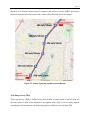
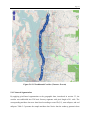
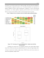
Figure 3-1 Data Acquisition Methods for the DRIVE Net System ...................................... 10 Figure 4-1 PostgreSQL, PostGIS, and pgRouting ................................................................ 21 Figure 4-2 DRIVE Net 3.0 Architecture ............................................................................... 23 Figure 4-3 High Resolution OpenStreetMap near the University of Washington ................ 26 Figure 4-4 Communication Mechanism for OpenStreetMap ............................................... 27 Figure 4-5 Multiple Layers on Top of a Map ....................................................................... 28 Figure 4-6 Travel Time Performance Measurement ............................................................. 29 Figure 5-1 Geospatial Data Fusion Challenge ...................................................................... 32 Figure 5-2 Vector Overlay .................................................................................................... 32 Figure 5-3 HCM2010 Modeling Framework........................................................................ 33 Figure 5-4 Image Resolution (Wikipedia, 2013) .................................................................. 34 Figure 5-5 Nearest Upstream and Downstream Ramps ........................................................ 37 Figure 5-6 HCM Speed-Flow Model (HCM, 2010) ............................................................. 40 Figure 5-7 Undersaturated, Queue Discharge, and Oversaturated Flow (HCM, 2010) ....... 42 Figure 5-8 I-5 Northbound Corridor (Tacoma - Everett)..................................................... 45 Figure 5-9 INRIX Speed, Adjusted Volume, and Density ................................................... 47 Figure 5-10 LOS by Phase 2.1 (without INRIX Speed Data) and Phase 2.2 (with INRIX
Speed Data) ................................................................................................................... 49 Figure 5-11 Training Set: Two Clusters by K-means Algorithm Analysis .......................... 51 Figure 5-122 User Interface Design...................................................................................... 52 Figure 5-133 Data Visualization: LOS Map ......................................................................... 53 Figure 6-1 Loop Data Quality Control Flow Chart .............................................................. 56 Figure 6-2 Imputation Using Adjacent Loop(s) on Multiple Lanes ..................................... 60 Page x
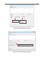
Figure 6-3 Imputation Using Upstream (Downstream) Adjacent Loops.............................. 61 Figure 6-4 GUI for Loop Data Error Detection .................................................................... 63 Figure 6-5 GUI for Loop Data Error Correction .................................................................. 63 Figure 7-1 MACAD Evolution ............................................................................................. 72 Figure 7-2 Bluetooth Data Collection and Distribution Diagram ......................................... 73 Figure 7-3 A Motorola Droid Handset Running the Mobile Monitor Ppplication (Phones
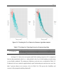
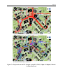
used in study courtesy of Dr. Alan Borning) ................................................................ 74 Figure 7-4 Trajectories on the UW Campus on April 20, 2011, 1:10pm to 2:00pm,
Collected by Four Observers ........................................................................................ 76 Figure 7-5 Inference of Plausible Paths ................................................................................ 79 Figure 7-6 Diagram of Route Imputation System................................................................. 80 Figure 7-7 Distance Threshold (in meters) for Certain/Uncertain Path Discrimination ....... 81 Figure 7-8 Imputed Plausible Paths from the Campus Experiment Conducted April 20,
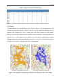
2011............................................................................................................................... 83 Figure 7-9 Static Sensor Mounting Locations on the University of Washington Campus ... 85 Figure 7-10 Comparison of Heatmaps of MAC Devices Detected on the UW Campus ...... 86 Figure 7-11 Ray Charts Depicting Pairwise Flows for Each Static Sensor Location ........... 88 Figure 7-12 Percentage of Correctly Matched MACs without and with Path
Reconstruction .............................................................................................................. 89 Figure 7-13 a) Percentage of Correctly Matched MACs by Distance Threshold with
Popularity Weights of 1250 to 5000 ............................................................................. 90 Figure 8-1 DRIVE Net Screen .............................................................................................. 91 Figure 8-2 DRIVE Net LOS Analysis Screen ...................................................................... 92 Figure 8-3 Summary LOS Analysis Screen .......................................................................... 93 Figure 8-4 WSDOT Region Map.......................................................................................... 93 Page xi
Figure 8-5 DRIVE Net Traffic Flow Map Screen ................................................................ 94 Figure 8-6 Traffic Flow Map Generated in DRIVE Net....................................................... 94 Figure 8-7 DRIVE Net Pedestrian Analysis Screen ............................................................. 96 Figure 8-8 DRIVE Net Gray Notebook Calculations Screen ............................................... 97 Figure 8-9 Travel Time Analysis Options (left) and Throughput Productivity Options ..... 97 Figure 8-10 Throughput Productivity Summary Statistics ................................................... 99 Figure 8-11 Throughput Productivity Graph for Northbound I-405 at SR 169, Based on
a Maximum Throughput Speed of 50 MPH ............................................................... 100 Figure 8-12 Travel Time Statistics Results for the Bellevue to SR 524 Corridor .............. 101 Figure 8-13 Stamp Graph for the Bellevue to SR 524 Corridor, Morning Period.............. 102 Page xii
Table of Tables
Table 3-1 20-Second Freeway Loop Data Description......................................................... 12 Table 3-2 5-Minute Freeway Loop Data Description ........................................................... 13 Table 3-3 Cabinet Data Description ..................................................................................... 14 Table 3-4 INRIX Data Description ....................................................................................... 15 Table 3-5 TMC Code Examples ........................................................................................... 15 Table 3-6 WITS Data Description ........................................................................................ 16 Table 3-7 Weather Data Description .................................................................................... 17 Table 5-1 Examples of Segmented I-5.................................................................................. 35 Table 5-2 Default Values for Basic Freeway Segments ....................................................... 38 Table 5-3 Speed-Flow Equations (HCM, 2010) ................................................................... 41 Table 5-4 LOS Criteria for Basic Freeway Segments .......................................................... 41 Table 5-5 Fused Attribute Data............................................................................................. 46 Table 5-6 LOC Count by Phase 2.1 (without INRIX Speed Data) and Phase 2.2 (with
INRIX Speed Data) ....................................................................................................... 48 Table 5-7 Training Set: Clustering Centers by K-means Algorithm .................................... 51 Table 5-8 Test Results .......................................................................................................... 52 Table 6-1 Data Quality Health Score Table .......................................................................... 58 Table 6-2 Error Type Summary for 20-Second Loop Data on October 14, 2013 ................ 59 Table 7-1 Observer Sensor Visit Itineraries.......................................................................... 86 Table 7-2 Relative Errors in Pairwise Flows for Mobile and Static Bluetooth Data ............ 89 Page xiii
Executive Summary
Traffic sensors have been widely deployed over the state highway network in Washington.
Additionally, more and more companies and agencies, such as INRIX, Inc., have developed
technologies that can extract “third party” traffic data from vehicle fleets and travel individuals.
These third party data greatly complement data from the traffic sensor network of the
Washington State Department of Transportation (WSDOT), particularly for rural areas where
traffic detectors are sporadic. The combined WSDOT data and third party data are huge in
volume and are highly valuable for system operations, monitoring, and analysis. However, the
current traffic data archive systems were designed mainly for data storage and off-line analysis.
They lack the capability to integrate third party datasets and do not offer the functions needed for
real-time performance monitoring, quick operational decision support, and system-wide analysis.
The goal of this study was to remove the barriers in the current datasets archived by
WSDOT, automate the time-consuming data quality control process, and achieve the integration
and visualization of information necessary to support decision making. The research findings are
not only summarized in this report, which describes the data fusion techniques and database
design details, but are also delivered in a functioning online system named WSDOT Digital
Roadway Interactive Visualization and Evaluation Network (DRIVE Net). This WSDOT DRIVE
Net system is capable of collecting, archiving, and quality checking traffic sensor data from all
WSDOT regions and incorporating third party data, such as those from INRIX, Inc., and weather
information into the analytical platform. Roadway geometric data are properly stored in an opensourced, geospatial database, and seamlessly connected with the traditional transportation
datasets. The existing WSDOT data archiving and analysis systems, CD Analyst and FLOW,
were successfully recoded and integrated into the WSDOT DRIVE Net system for better
efficiency and consistency. A series of loop data quality control algorithms, including basic
thresh-holding, Gaussian Mixture Model (GMM), and spatial/temporal correction, are automated
in the backend for detecting malfunction loops and correcting them whenever possible.
A variety of datasets, including freeway loop data, INRIX GPS, Washington Incident
Tracking System (WITS), and weather data, are incorporated and archived into well-designed
databases. Unlike other prevailing transportation data archiving systems, DRIVE Net is also
capable of processing and storing massive amounts of spatial data by using open-sourced spatial
Page xiv
database tools. This significantly alleviates the computational and financial burden of using
commercial geographic information system (GIS) software packages and grants maximum
flexibility to end users. By properly combining both traditional transportation and spatial data, a
more robust GIS-T model is available for large-scale modeling and network-level performance
measures following eScience principles.
To develop a more stable yet interoperable platform to process, analyze, visualize, and
share transportation data, the previous version of the DRIVE Net system, developed through
voluntary efforts, was remodeled by incorporating multiple open-sourced software tools such as
OpenStreetMap, OpenLayers, and the R statistics package. The new DRIVE Net system is built
over a fat-server, thin-client framework. It requires no additional installation efforts for users.
Moreover, its security and reusability are significantly better than the previous design. The new
DRIVE Net system is now able to handle more complex computational tasks, perform largescale spatial processing, and support data sharing services.
With the new data platform empowered by eScience transportation principles, two
commonly utilized functions at WSDOT were implemented to demonstrate the efficiency and
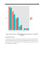
utility of this new system. The first function was to generate WSDOT’s Gray Notebook statistics
and charts. Cleaned data were utilized to generate statistics for WSDOT’s Gray Notebook. The
calculated statistics were presented on an interactive map system. This new function will allow
WSDOT personnel to produce the tables and figures needed for their annual and quarterly
congestion reports in seconds, a significant improvement over the months previously necessary.
The other function was the level of service (LOS) map for highway performance
assessment. This module follows the Highway Capacity Manual (HCM) 2010 procedure to
produce an LOS estimate for each roadway segment every 20 seconds on the basis of real-time
traffic measurements. To implement this approach, the research team developed a spatial data
fusion technique, pixel-based segmentation, and used it to spatially overlay multi-level geometric
data and transportation data. Roadway geometric data, GPS probe vehicle-based speed data from
INRIX, and fixed traffic sensor data were fused in our calculation process. This new LOS
calculation approach was compared with several other algorithms, and the results proved it to be
accurate and efficient.
Page xv
Additionally, a mobile sensing data analysis module was developed as a pilot experiment
for reconstructing pedestrian/bicyclist trajectories by using the Media Access Control (MAC)
addresses captured from mobile devices. Each pedestrian/bicyclist with a Bluetooth-enabled
mobile device was considered to be a moving sensor. Data observers with our phone app
designed for collecting Media Access Control (MAC) addresses from mobile device Bluetooth
signals recorded MAC addresses and the time when they were observed. These MAC addresses
and timestamps were then sent to the STAR Lab server for processing to extract trajectory
information. Given the lack of pedestrian/bicyclist movement data and the challenges to collect
them, this pilot experiment may have introduced a new and cost-effective method for collecting
such data.
In summary, this study shed light on the development of an eScience transportation
platform and provided an interoperable data-driven online tool to substitute for WSDOT’s
existing data systems. The major merits and contributions are listed below:
(1) The DRIVE Net system is significantly enhanced with multiple open-sourced
software packages and a robust system design.
(2) This study developed an efficient and effective GIS-T model to integrate massive
amounts of transportation data from various sources into the roadway network.
(3) WSDOT’s existing data systems (CD Analyst and FLOW) are successfully
incorporated into the DRIVE Net system.
(4) More heterogeneous datasets, including INRIX speed data, weather data, and WITS
data, have been imported into the DRIVE Net system. The loop sensor data coverage
is also greatly expanded.
(5) The WSDOT Gray Notebook has been included as a key component in the DRIVE
Net system. The raw loop data are preprocessed through a series of rigorous data
quality control processes in an automatic manner and are further imported for
congestion statistics calculation. The generated statistics are presented on a digital
map system for reporting and visualization.
(6) The HCM 2010 Level of Service (LOS) module is automated in DRIVE Net. INRIX
data, loop detector data, and roadway geometric data are fused with a spatial fusion
approach, then the K-means clustering algorithm and regression technique are jointly
applied to predict LOS for real-time freeway performance monitoring.
Page xvi
(7) A mobile sensing data analysis framework has been developed. This framework
includes a prototype mobile phone app for MAC address data collection, a pedestrian
trajectory reconstruction algorithm, and a computer module in DRIVE Net that
implements the trajectory reconstruction algorithm.
Future endeavors can be undertaken to expand the scope of DRIVE Net to the entire
state, design an analytical module for quantifying the benefits of ATM and management lanes,
conduct safety performance measurements, and more.
Page 1
Chapter 1 Introduction
1.1 Problem Statement
The Washington State Department of Transportation (WSDOT) is facing increasing demands on
its data infrastructure. Accountability, operations, environmental impact analysis, system design,
and implementation decisions require data-driven and data supported decision making. Data and
support tools need to be accessible to WSDOT personnel for reporting and public outreach
purposes. These include functionalities currently offered by legacy applications such as CD
Analyst, databases such as the FLOW archive, and applications to be developed for
accountability, operations, and design decision support.
The problem with the FLOW archive and CD Analyst functions that are currently widely
used within WSDOT is that they were created almost 20 years ago. They were advanced and
efficient when they were designed, but they are simply outdated and are now architecturally
awkward and generally unsuited for combination with new functions. Computing power,
programming models, Internet functionality, and electronic maps have advanced a great deal
since FLOW and CD Analyst were first coded. Now a dynamic, visual, and multiple datasetbased decision making support tool is well within technical means. Given increasing data
analysis needs and aging infrastructure, it is time to refresh WSDOT’s current data infrastructure
and analytical tools.
Because of their age, the current legacy data archival and analysis tools are unable to
answer decision support questions related to operations strategies, design requirements, and
increased public scrutiny. For example, new traffic control and design decisions, such as those
involved with active traffic management (ATM), will require new applications and databases for
decision support. Some ATM strategies, such as demand management via tolling and variable
speed limits, have very high public visibility.
They also span large areas and can affect
infrastructure across multiple jurisdictions. Design, operations, and accountability decisions for
such large-scale projects require data input from multiple sources, algorithms to compute
Page 2
performance measures, and efficient communications media such as maps, charts, and reports.
However, the WSDOT existing data systems are not capable of integrating multiple data sources.
In addition, with the current data archival and analysis tools, assessments of operational
performance and future implementation decisions must be performed manually. For example, for
performance measures, such as incident rates related to variable speed limit, incident times from
the Washington Incident Tracking System (WITS) databases must be matched to variable speed
limit records along with any other traffic data of interest, such as volumes and speeds.
Generating useful performance measures and analysis is labor intensive and time consuming
because of the lack of a suitable platform to process and deliver transportation information
efficiently, and thus, limits the WSDOT’s ability to respond to legislative and agency requests.
A potential answer to the problems posed by the current databases is a prototype Webbased analytical framework called the Digital Roadway Interactive Visualization and Evaluation
Network (DRIVE Net). Developed at the University of Washington (UW) Smart Transportation
Applications and Research Laboratory (STAR Lab), DRIVE Net, as it has come to be known, is
a first step in attempting to tie together the multiple sources of transportation-related data that are
quickly becoming available. A key aspect of the system is an interface that allows sensor data to
be overlaid on OpenStreetMap, providing immediate visual representation and analysis. Trends
and correlations that would otherwise be concealed in tables become visually apparent when
overlaid on a map. Additionally, the OpenStreetMap-based spatial organization of data provides
an intuitive interface that is familiar to many users. DRIVE Net is part of a new trend in datadriven decision-making support tools by including data from WSDOT’s Northwest Region, the
City of Bellevue, and several other entities. However, the functionalities of the current DRIVE
Net are limited. The STAR Lab envisions addressing WSDOT’s needs by further developing
DRIVE Net, not only taking advantage of all WSDOT regions’ data and the existing functions of
CD Analyst, but also providing a platform for
transportation data management, analysis,
visualization, and decision making.
1.2 General Background
The concept of a statewide data network is not a new one. Several examples exist, such
California’s Performance Measurement System (PeMS) and Oregon’s Portland Oregon Regional
Transportation Archive Listing (PORTAL). The original model for these systems is similar to the
Page 3
CD-based archive developed in the early 1990s by the Washington State Transportation Center
(TRAC) – the FLOW system.
Because of the era during which it was developed, the FLOW system is not a fully
functional relational database. It is a series of flat files that are manipulated through a series of
stand-alone programs. The stand-alone programs are designed to read those files and produce
secondary files. The secondary files are read into additional programs—including conventional
spreadsheets containing basic Macro functionality, which in turn produce a variety of analytical
outputs used by WSDOT. The combined series of analytical programs goes by the name of CD
Analyst.
The CD Analyst suite of programs has been developed over an 18-year period. It
produces a large number of key accountability reports for WSDOT and also performs the basic
analysis of freeway performance reporting for WSDOT. Unfortunately, the CD Analyst suite of
programs has grown organically over that 18-year period, with that growth always focused on
the provision of new analytical capabilities needed to meet specific WSDOT reporting needs.
Because available funds have always been focused on adding specific analytical capabilities, the
inherent data structure has never been modified to allow easier and more flexible access to the
collected data.
As a consequence, the system has not taken advantage of many of the
improvements in computing technology which have occurred since the mid-1990s. The result is
that, while the current WSDOT data system functions, it is neither as efficient nor as flexible or
accessible as needed.
The DRIVE Net system has evolved from two major STAR Lab research efforts, the
Google-map-based Arterial Traffic Information (GATI) system (Wu, 2007) and the
Development of a Statewide Online System for Traffic Data Quality Control and Sharing (Wang
et al., 2009) project sponsored by the WSDOT and Transportation Northwest (TransNow).
Freight management functions have been added through the Developing a GPS-based Truck
Performance Measures Platform (McCormack, 2010) project sponsored by WSDOT and
TransNow. Additional datasets and modules have been added on a test basis. These modules are
generally operating on a reduced number of datasets, because of either data availability or
analysis complexity. Test modules include freeway level of service (LOS) and link emissions
mapping applications.
Page 4
The DRIVE Net framework is designed upon a scalable and modular architecture. This
architecture is intended to make the addition of various analytical modules as easy as possible so
that future upgrades will require minimal effort. A series of Extract, Transform and Load (ETL)
programs collect, format, and store the data in the appropriate databases. As new data sources are
added, existing ETL tools can be adopted if the data source is similar to an existing data source,
or new ETL logic can be written as needed. Once data have been loaded into databases, many
data formatting inconsistencies, such as collection periods, can be reduced through database
functions and aggregation within queries. This allows analyses at a flexible resolution level while
maintaining compatibility with established 5-minute based analyses, such as those conducted by
CD Analyst.
DRIVE Net has also been designed from the beginning to present analytical results in a
visual and map aware manner. This allows functions such as the emissions model to take
underlying traffic data, apply a traffic emissions model, and then display a color-coded map for
viewing the results. This ability will allow the current functionalities of CD Analyst, as well as
future functionalities, to be visualized.
The addition of other datasets, such as WITS, weather, and INRIX data, will provide new
analytical and data quality control options. Incident data from these sources can be used to flag
affected analyses in order to reduce inaccuracies due to abnormal traffic. Simply flagging results
that may be affected by incidents that happened on the selected route(s) at the selected time(s)
could have profound implications for the quality of data analyses.
1.3 Research Objectives
The primary goal of this study is to provide a data-driven, online transportation platform as a
substitute for the previous CD Analyst to provide WSDOT Gray Notebook statistics calculations
and to incorporate more diverse and heterogeneous sensor data sources. In addition, DRIVE Net
will be able to automate the Highway Capacity Manual (HCM) 2010 method calculations for
freeway performance measures and to implement a mobile sensing data analysis framework for
reconstructing pedestrian trajectories. This e-Science platform will not only serve to archive the
tremendous amount of historical transportation data, but will also provide several visualization
and modeling tools to help users better understand the large sets of transportation data, and thus
make more informed decisions. The detailed research objectives are listed below:
Page 5

Enhance the current DRIVE Net system by improving system design and increasing
sensor data coverage.

Integrate WITS, weather, and INRIX data into DRIVE Net and apply them for analytical
functions.

Expand the current data coverage of freeway loop detectors statewide.

Incorporate CD Analyst functions into DRIVE Net by re-coding its core functions.

Develop an automated function to compute statistics and charts needed to produce the
WSDOT Gray Notebook.

Develop an example module to show how DRIVE Net’s databases and analytical
functions may be applied to measure freeway performance with the HCM 2010 method.

Develop a mobile sensing data analysis framework with a prototype mobile phone app
for MAC address data collection and pedestrian trajectory reconstruction.
Page 6
Chapter 2 Literature Review
In the past decades, a considerable number of online transportation platforms for data sharing,
archiving, and analysis have been developed for transportation agencies and the public. Typical
examples of them are described as follows:
2.1FreewayPerformanceMeasuresSystems(PeMS)
Established in 1998, PeMS is a freeway performance measurement system jointly
developed by the University of California, Berkeley, California Department of Transportation
(Caltrans), and the Partners for Advanced Transportation Technology (PATH). With support
from Caltrans and local agencies, the system integrates various traffic data sources, including
traffic detectors, census traffic counts, incident logs, vehicle classification data, toll tag-based
data, and roadway inventory. These traffic data have been automatically collected and archived
for over ten years, and real-time information is updated from over 25,000 detectors (Chen et al.,
2001; Chen et al., 2003). As a critical component of Caltrans performance measurement system,
PeMS provides a variety of freeway evaluations in terms of speed, occupancy, travel time,
vehicle miles traveled, vehicle hours traveled, and vehicle hours of delay. The success of PeMS
for freeways has triggered the development of a similar system for arterial performance
evaluation. Following the basic principle of PeMS, the Arterial Performance Measurement
System (APeMS) has been implemented to estimate intersection travel time, control delay, and
progression quality on arterials every 5 minutes by using mid-block loop detectors (Tsekeris et
al., 2004; Petty et al., 2005). Unlike the open availability of PeMS, APeMS usage is designated
for stakeholders, and it is not accessible by the public.
2.2RegionalIntegratedTransportationInformationSystem(RITIS)
RITIS is an automated data archiving and integration system developed by the Center for
Advanced Transportation Technology Laboratory (CATT Lab) at the University of Maryland.
The focus of RITIS, one of several online transportation archive systems, is to improve
transportation safety, efficiency, and security by fusing and mining transportation-related data in
Maryland, Virginia, and the District of Columbia. The system provides both real-time and
historical data to users with access credentials, including incident, weather, radio scanner, and
Page 7
other sensor data. Numerous visualization and analysis tools have been developed to enable
interactive exploration and analysis of performance measures from archival data. DOT or public
safety employees can possibly use the RITIS service by applying online. The system is not
accessible to the general public (CATT lab, 2013).
2.3Portland,Oregon,RegionalTransportationArchiveListing(PORTAL)
Originally established in 2004 with a simple user interface and only one data source—
freeway loop detectors—PORTAL has evolved significantly over the past eight years. In
addition to the loop detector data from the Portland-Vancouver metropolitan region, PORTAL
2.0 now archives approximately 1 terabyte of transportation data, including weather, incident,
freight, and transit data. The system takes advantages of Adobe Flash and Google Maps
technologies to display transportation data spatially. Additionally, various graphical and
tabulated performance information is available on the website, such as incident reports, transit
speed maps, traffic counts, vehicle miles traveled, and vehicle hours traveled (Tufte et al., 2010).
2.4FreewayandArterialSystemsofTransportation(FAST)Dashboard
The FAST dashboard, released online in September 2010 (http://bugatti.nvfast.org), is a
Web-based system developed to control and monitor traffic in the Las Vegas and Nevada
metropolitan areas (Xie and Hoeft, 2012). In collaboration with the Nevada Department of
Transportation (NDOT), the system collects and archives real-time traffic data retrieved from
loop detectors, radar detectors, and Bluetooth sensors deployed on freeways and ramps. Traffic
data including lane occupancy, volume, and speed data are further processed as the major data
sources for performance measurement. Also integrated into the system are incident data in report
format collected from the general public, and weather data shared by the NDOT Road Weather
Information System.
The performance measures used by the FAST dashboard include average speed,
traditional travel time performance measures, delay volume, and temporal and spatial extension
of congestion. Meanwhile, the website is updated every 1 minute to display the real-time traffic
map. By ensuring the delivery of timely and accurate information to traffic managers, operators,
and planners as well as the general public, the FAST dashboard significantly enhances the
interchangeability of traffic data, helps improve the freeway and arterial system, and optimizes
operation strategies in the southern Nevada region.’
Page 8
2.5ApplicationsinWashingtonState
In Washington state, a great effort has also been made to develop applications to supply traffic
data for traffic monitoring and research activities. Completed in 2002, The Traffic Data
Acquisition and Distribution (TDAD) project provided a traffic data repository for a chosen wide
area, such as King County in Washington. The interactive user interface enabled transportation
researchers and agencies to query historical data by time and location. This was not very
common in the early 21st century.
Established in 2006, the DRIVE Net system has evolved from two major STAR Lab
research projects, the Google-map-based Arterial Traffic Information (GATI) system (Wu, 2007)
and the Development of a Statewide Online System for Traffic Data Quality Control and Sharing
(Wang et al., 2009) project sponsored by WSDOT and Transportation Northwest (TransNOW),
the USDOT University Transportation Center for federal region 10. In 2008, the system was
named the Digital Roadway Interactive Visualization and Evaluation Network (Ma et al., 2011).
More functions have been implemented and integrated into the system over time, such as a
freight management module (Ma et al., 2011), incident induced delay calculations (Yu et al.,
2013), arterial travel time estimation (Wu et al., 2011) and emission data analysis (Ma et al.,
2012). DRIVE Net provides users with the capability to store, access, and manipulate data,
which benefits not only transportation practitioners and researchers but also the public by
providing both historical and real-time transportation information and numerous performance
measures in the broader context of an interdisciplinary framework.
Page 9
Chapter 3 Study Data
DRIVE Net builds upon existing databases controlled by the STAR Lab. A variety of data
sources are digested and archived into the STAR Lab server from WSDOT and third party data
providers through different data acquisition methods.
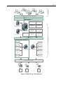
There are four ways to use the data archive service, as illustrated in Figure 1:
1. Direct upload
Users can upload data into the database through the DRIVE Net website. This model is
suitable for receiving data from those who do not maintain online databases. Typical datasets
used in this study include INRIX data and weather station data.
2. Periodic download via Web services
A scheduled fetch job is run to download data at predefined intervals via File Transfer
Protocol (FTP), Hypertext Transfer Protocol (HTTP), Simple Object Access Protocol (SOAP), or
Representational State Transfer Principles (RESTful) interfaces. This method is currently used
for the acquisition WSDOT freeway loop data.
3. Active data acquisition
For those agencies with specialized needs or who do not allow public access, the research
team will construct a satellite server—a form of “information appliance”—bundling hardware,
software, and data processing services into a single provisionable platform. These satellite
servers elegantly solve several problems related to bootstrapping a data sharing network. First,
system administrators rarely create holes in their firewalls for connections with remote machines.
The appliance, however, can be deployed inside the agency’s firewall and still connect to remote
servers by using port 80 or port 22, which are usually unrestricted. Second, specialized software
for establishing a Web service, in order to use the periodic download method, is difficult to
install and configure. Even if a comprehensive software suite is written, the cost of providing
technical support to users would be prohibitive. However, installing the software on behalf of a
customer on computers over which the STAR Lab has complete control is far more
straightforward. Finally, the appliance grants access to STAR Lab researchers and technicians as
well as participant agency staff. This allows multi-agency shared access, which can simplify
Page 10
troubleshooting and upgrade deployment. This method is currently used to retrieve the roadway
geometric data and WITS data from WSDOT.
4. Direct data archiving
The data are generated from the data collection devices and enter into the data warehouse
by several communication protocols, such as General Packet Radio Service (GPRS) and Global
System for Mobile Communications (GSM). Mobile sensor data are transmitted into DRIVE Net
with this method.
Figure 3-1 Data Acquisition Methods for the DRIVE Net System
Detailed information about each data source is described in the following sections.
3.1 Freeway Loop Data
Inductive loop detectors are widely used to monitor freeway performance in the United States
because of their reliability and durability (Klein et al, 2006). An inductive loop detector is a
conductive coil embedded in the pavement, and it detects a moving vehicle passing over it with
electromagnetics. The signal is then transmitted to a roadside cabinet, which stores the vehicle
presence information and also sends the signal to the traffic management center via cable.
Volume and occupancy are two key indicators that traffic detectors can collect during a fixed
Page 11
time interval (20 seconds or 5 minutes). WSDOT maintains and manages loop detectors in both
Washington state highway and Interstate freeways. Washington divides the state into six regions:
Northwest, North Central, Eastern, South Central, Southwest, and Olympic. For instance, there
are approximately 4200 single or dual loop detectors installed in the Northwest Region, and they
aim to monitor traffic condition around the Seattle metropolitan area.
WSDOT stores both 20-second and 5-minute loop detector data using an online FTP
website for downloading. The 5-minute loop detector data are aggregated from 20-second loop
data for long-term analysis and archiving. A computer program written in Microsoft Visual C#
was developed to periodically retrieve loop data from the posted FTP website, and the
downloaded data are automatically imported into Microsoft SQL server databases for further
processing.
Single loop detectors can detect only whether a vehicle is present or absent. When several
vehicles pass over a single loop detector during a certain time interval, the detector is able to
count the number of vehicles and the percentage of time when the detector is occupied. Unlike
single loop detectors, a dual loop detector is composed of two single loop detectors, which are
placed a short distance apart. By measuring the arrival time difference between the two loops,
the roadside traffic controller can calculate each vehicle’s speed. The vehicle’s length can be also
estimated by using the calculated vehicle speed and the on-time measurement from either the
front loop or the rear loop.
For both 20-second and 5-minute data aggregation intervals, three types of loop data are
collected. The key information is listed in Table 3-1 and Table 3-2.
Page 12
Table 3-1 20-Second Freeway Loop Data Description
Table: SingleLoopData and StationData (Single Loop)
Columns
Data Type
Value Description
LOOPID
smallint
Unique ID number assigned in order of addition to
LoopsInfo table
STAMP
datetime
24-hour time in integer format as YYYYMMDD hh:mm:ss
(in 20-second increments)
DATA
tinyint
Indicate whether a record is present or not
FLAG
tinyint
Validity flag (0-7): 0=good data; otherwise, bad data
VOLUME
tinyint
Integer volume observed during this 20-second interval
SCAN
smallint
Number of scans when a loop is occupied during each period
(60 scans per second multiplied by 20 seconds per period
equals 1200 scans)
Table: TrapData (Dual Loop)
Columns
Data Type
Value Description
SPEED
smallint
Average speed for each 20-second interval (e.g., 563 means
56.3 mile per hour)
LENGTH
smallint
Average estimated vehicle length for each 20-second interval
(e.g., 228 means 22.8 feet)
WSDOT primarily uses the 5-minute aggregation level loop data for freeway
performance measures (Wang et al., 2008). The key information for 5-minute loop data is shown
in Table 3-2.
LoopID is the unique ID that matches each cabinet with loop data. Several loops could
connect to each cabinet. For each cabinet, these loop data are aggregated as a loop group, namely
a loop station, for which the volume is the sum of total volumes for the associated loops, and the
occupancy (or scan) is the average of total occupancies (scans) for the associated loops. In
addition, to facilitate locating and categorizing each loop, each loop is assigned to a cabinet with
spatial information (e.g., milepost). The key information is listed in Table 3-3.
Page 13
Table 3-2 5-Minute Freeway Loop Data Description
Table: STD_5Min and STN_5Min (Single Loop)
Columns
Data Type
Value Description
LOOPID
smallint
Unique ID number assigned in order of addition to
LoopsInfo table
STAMP
datetime
24-hour time in integer format as YYYYMMDD hh:mm:ss
(increased by 5 minutes)
FLAG
tinyint
Good/bad data flag with 1 = good and 0 = bad (simple
diagnostics supplied by WSDOT)
VOLUME
tinyint
Integer volume observed during each 5-minute interval
OCCUPANCY
smallint
Percentage of occupancy expressed in tenths to obtain
integer values (6.5% = 65)
smallint
The number of 20-second readings incorporated into this 5minute record (15 is ideal, less than 15 almost always
indicates that volume data are unusable unless adjusted to
account for missing intervals).
PERIODS
Table: TRAP_5Min (Dual Loop)
Columns
Data Type
Value Description
SPEED
smallint
Average speed for each 5-minute interval (e.g., 563 means
56.3 mile per hour)
LENGTH
smallint
Average estimated vehicle length for each 5-minute interval
(e.g., 228 means 22.8 feet)
Page 14
Table 3-3 Cabinet Data Description
Columns
Data Type
Value Description
CabName
varchar
Unique ID for each cabinet
UnitType
varchar
Type for each loop (i.e. main, station, speed and trap)
ID
smallint
Unique ID number assigned in order of matching the loop
data table
Route
varchar
The state route ID (e.g. 005=Interstate 5)
direction
varchar
Direction of each state route
isHOV
tinyint
Bit indication whether loop detector is on an HOV lane
(1=HOV, 0=not HOV)
isMetered
tinyint
Bit indication whether loop detector is on a metered ramp
(1=metered, 0=not metered)
Although WSDOT provides a preliminary data quality assurance procedure to flag
erroneous loop data, this procedure is still unable to capture other possible errors, such as loop
detector sensitivity issues (Corey et al., 2011). Because of the environmental changes around
loop detectors over time, the actual detection zone of these loops may increase or decrease, and
these changes will consequently affect the accuracy of speed calculations. Zhang et al. (2003)
stated that approximately 80 percent of WSDOT dual-loops suffer from severe sensitivity
problems. It is of critical importance to detect and correct possible loop errors before conducting
freeway performance measurement. A detailed loop data quality control mechanism will be
discussed later in this report.
3.2 INRIX Data
As a leading traffic data provider, INRIX combines multiple data sources, including GPSequipped devices and cell phones. INRIX tracks more than 30 million probe vehicles and more
than 400 additional data sources (INRIX, 2012).
To aggregate and fuse heterogeneous
transportation data, INRIX developed a series of statistical models to compute real-time traffic
information such as speed and travel time based on measurements from GPS devices, cellular
networks, and loop detectors. The resulting speed data were aggregated into 5-minute intervals
Page 15
for 2008, 2009, and 2010 and into 1-minute intervals for 2011 and 2012. WSDOT purchases the
data, and they are further archived into the database in the STAR Lab. INRIX data cover almost
the entire roadway network in Washington, including freeways, highways, and most arterials and
side streets. The key information for INRIX data is presented in Table 3-4.
Table 3-4 INRIX Data Description
Columns
Data Type
Value Description
DateTimeStamp
datetime
24-hour time in integer format as YYYYMMDD hh:mm:ss
SegmentID
varchar
Unique ID for each segment-Traffic Message Channel
(TMC) code
Reading
smallint
Average speed for each segment
INRIX has adopted the Traffic Message Channel (TMC), a common industry convention
developed by leading map vendors, as its base roadway network. Each unique TMC code is used
to identify a specific road segment. For example, in Table 3-5, TMC 114+0509 represents the
WA-522 road segment with start location (47.758321, -122.249705) and end location
(47.753417, -122.277005). However, that fact that WSDOT follows a linear referencing system
based on mileposts poses challenges to matching the two different roadway layouts for data
fusion.
Table 3-5 TMC Code Examples
TMC
Roadway
Direction
Intersection
Country
Zip
Start Point
End Point
Miles
114+05099
522
Eastbound
80th Ave
King
98028
47.758321,122.249705
47.755733,122.23368
0.768734
114-05095
522
Westbound
WA523/145th St
King
98115
47.753417,122.27005
47.733752,122.29253
1.608059
3.3 WITS Data
Traffic incident data are collected and maintained by Washington State’s Incident Response (IR)
Team in the Washington Incident Tracking System (WITS). WITS includes the majority of
Page 16
incidents that happen on freeways and Washington state highways, which totaled 550, 376 by
March 2013. For each incident, the Washington State IR team logs details such as incident
location, notified time, clear time, and closure lanes. The DRIVE Net team obtained the WITS
datasets from 2002 to 2013 and integrated them into the DRIVE Net database. Several key
columns are listed in Table 3-6.
Table 3-6 WITS Data Description
Columns
Data Type
Value Description
SR
varchar
State route ID, e.g., 005=Interstate 5
Direction
varchar
Route direction (NB=northbound, SB=southbound,
WB=westbound, EB=eastbound)
MP
float
Milepost
Notifited_Time
datetime
The time when an incident was reported to the Incident
Response (IR) program
Arrived_Time
datetime
The time when an IR truck arrived at the incident
location
Clear_Time
datetime
The time when the incident had been fully cleared and
all IR crews left the incident scene
Open_Time
datetime
The time when all lanes became open to the traffic and
IR crews may still be on the incident scene
3.4 Weather Station Data
Weather data are retrieved from the National Oceanic and Atmospheric Administration (NOAA)
weather stations in the region. The University of Washington Atmospheric Sciences Department
hosts a website that records all the weather statistics from 209 weather stations in Washington
state every hour. The DRIVE Net team developed a Java-based computer program to fetch the
weather report in an automatic manner through the HTTP connection. The retrieved data are then
imported into a database in the STAR Lab. The key information of the weather data is shown in
Table 3-7.
Page 17
Table 3-7 Weather Data Description
Columns
Data Type
Value Description
name
varchar
The weather station identifier
timestamp
datetime
24 hour time in integer format as YYYYMMDD hh:mm:ss
visibility
smallint
Visibility in miles
temp
smallint
Temperature in degrees Fahrenheit
dewtemp
smallint
Dewpoint temperature
wind_direction
smallint
Direction wind is coming from in degrees; from the south is
180
wind_speed
smallint
Wind speed in knots
pcpd
smallint
Total 6-hr precipitation at 00z, 06z, 12z and 18z; 3-hr total
for other times. Amounts in hundredths of an inch.
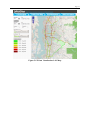
Each weather station is associated with a pair of latitude and longitude. In this case,
weather data can be visualized on a mapping system.
3.5 Roadway Geometric Data
WSDOT’s GIS and Roadway Data Office (GRDO) produces and maintains the GeoData
Distribution
Catalog
online
at
http://www.wsdot.wa.gov/mapsdata/geodatacatalog/.
The
geospatial data in the format of an ESRI Shapefile is available to the general public, promoting
data exchange and data sharing. Various roadway geometric datasets are available, including
number of lanes, roadway widths, ramp locations, shoulder widths, and surface types. State route
ID and locations marked by mileposts and accumulated mileage are also included in the WSDOT
linear referencing systems. For DRIVE Net, these geometric data were stored in a spatial
database for further processing. It is critical to connect roadway geometric data with traditional
transportation data. Chapter 4 discusses such a geospatial platform to undertake this task.
3.6 Mobile Sensing Data
The DRIVE Net team developed an in-house Bluetooth sensor, also known as the Media Access
Control Address Detection System (MACAD). Bluetooth is a short-range communication
Page 18
protocol initiated by Spatial Interests Group (SIG) for inter-device communications. Nowadays,
more and more electronic manufacturers embed such technology into their products. The
protocol utilizes a unique 48-bit Media Access Control (MAC) address to distinguish different
devices. Because earlier Bluetooth technology adopted a frequency-hopping protocol for device
discovery, the devices create a detection overhead of up to 10.24 seconds, causing spatial errors
in detection and therefore travel time measurements. A detailed description of the Bluetoothbased data technology is covered in Chapter 7.
A communication module is incorporated into our designed Bluetooth data collection
devices.. This module synchronizes to Coordinated Universal Time (UTC) over the GPS network
and transfers latitude and longitude to the server through the Global System for Mobile (GSM)
cellular system. Therefore, the key information from Bluetooth devices includes a timestamp, a
pair of geospatial coordinates, and a unique MAC address. To conduct further travel time
estimation or pedestrian tracking tasks, MAC address matching must be conducted.
Page 19
Chapter 4 DRIVE Net 3.0: System Design and Implementation
Despite many years of development, several challenging problems remained unsolved in the
previous version DRIVE Net 2.0. One critical issue was that the earlier versions had little geoprocessing power, which made it difficult to store, analyze, and manipulate geographic data.
Previous solutions included manually recording series of spatial locations (latitude and
longitude) for lines and polygons in a relational database. However, this ad hoc method was
inefficient, unreliable, and did not meet the needs of modeling complex spatial relationships.
Additionally, DRIVE Net 2.0 had severe bugs and was vulnerable to massive page visits
because of incompatibility issues among the development tools. Google Web Toolkit (GWT),
one of the major tools adopted in this earlier version, allowed developers to write in Java, and the
GWT compiler translated Java code into JavaScript. Although GWT is a widely used tool for
developing JavaScript front-end applications, it has a steep learning curve and requires
developers to constantly keep up with new technologies. Huge amounts of time and effort are
demanded to maintain and update the system because of the rapidly changing features of the
GWT. Therefore, a more productive and straightforward development process was desired to
ensure the stability of such online platforms. Another concern related to the inclusion of Google
Maps in DRIVE Net 2.0 was the licensing model revision announced by Google, Inc. in early
2012 (Google, 2012). It stated that only the first 2,500 geocoding Web services would be offered
free daily. Access to Google Maps would not be granted if a system continuously exceeded
usage limits. Therefore, potential maintenance costs forced the developers to change the DRIVE
Net system to a more flexible yet reliable alternative Web-mapping product, such as OpenLayers
and OpenStreetMap (OpenLayers, 2013; OpenStreetMap, 2013). These led to the development
of DRIVE Net 3.0, described in this section.
4.1 Geospatial Database Design
Because of the increasing amount of study data, multiple servers are configured to archive these
data. To better balance computational resources and allow fast data access, transportation data
and geospatial data are stored separately. The transportation data are managed by Microsoft SQL
Server 2010, and all the databases are indexed and optimized on the basis of projected needs.
However, the traditional method for handling geospatial datasets is to utilize commercial GIS
Page 20
software packages. Unfortunately, transportation agencies have to spend considerable amounts of
time and financial resources purchasing and maintaining the software (Sun et al., 2011). In
addition, because most commercial software is not designed as open architecture, transportation
agencies have to provide the spatial data in strict accordance with the format of GIS files used by
the commercial software. These restrictions incur inconveniences and reduce flexibility for both
users and developers. Moreover, file-based data management systems have inherent
disadvantages for processing tremendous amounts of data efficiently. Fortunately, the emergence
of new geospatial database techniques can alleviate the burden of file-based geospatial data
management and analysis. Similar to the traditional Relational Database Management System
(RDBMS), geospatial databases can optimize the geospatial data management and analysis by
using Structured Query Language (SQL) techniques and spatial indices. In addition, geospatial
databases enable a variety of geo-processing operations that traditional relational, non-spatial
databases cannot complete—for example, whether two polylines intersect, or whether points fall
within a spatial area of interest. For this study, non-spatial relational databases were used to store
traffic-related information such as loop detector data and INRIX data. This created a critical
issue: how to best represent and manage the dynamic transportation data in a context of hybrid
spatial and non-spatial databases. Especially when more and more location-aware transportation
data are available for advancing Big Data initiatives, this issue is becoming more pressing.
For the new system, PostgreSQL with extender PostGIS and pgRouting was adopted to
maintain geo-data and perform spatial modeling, as outlined in Figure 4-1. Those three products
are all free, open source, and well-supported by their active communities. Although some
commercial software such as ArcGIS/ArcServer could perform the same jobs, open source
projects are generally more academic in nature, despite the fact that commercial products usually
have expensive license and usage restrictions. The rest of this section introduces more details
about PostgreSQL, PostGIS, and pgRouting.
Page 21
extender
PostGIS
PostgreSQL
pgRouting
Figure 4-1 PostgreSQL, PostGIS, and pgRouting
PostgreSQL is a sophisticated and feature-rich object-relational database management
system under an open source license (PostgreSQL, 2013). Its powerful functions and efficient
performance make it the most popular open source database, and it is able to compete against
well-known commercial products such as Oracle, IBM DB2, and Microsoft SQL server. Some
advanced and unique features distinguish it from others, including table inheritance, support for
arrays, and multiple-column aggregate functions. Moreover, the active global community of
developers continually updates PostgreSQL with the latest database technology.
With PostgreSQL as a tabular database, PostGIS is a spatial database extender built on
PostgreSQL (Obe, 2011). The PostgreSQL/PostGIS combination offers support to store,
maintain, and manipulate geospatial data, making it one of the best choices for spatial analysis.
Besides the geo-data storage extension, PostGIS has nearly 300 geo-processing operators or
functions. The ability to analyze geographic data directly in the database by SQL sets
distinguishes PostGIS from commercial competitors. For example, the following spatial query
creates a polygon buffer with a size of 10,000 feet:
Select ST_Buffer(the_geom, 10000) from county_polygon
pgRouting is an extension of PostGIS/PostgreSQL geospatial database that provides a set
of routing-related SQL functions (pgRouting, 2013). Various routing algorithms are supported
Page 22
by pgRouting, including shortest path Dijkstra (Dijkstra, 1959), shortest path A* (Hart et al.,
1968), shortest path shooting*, traveling salesperson problems, and driving distance calculation.
Meanwhile, its open source framework makes it convenient for developing and implementing
user-specified routing algorithms. More advanced algorithms such as Multimodal Routing
support, Two-Way A*, and time-dependent/dynamic shortest path will be included in the near
future.
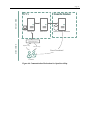
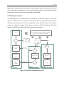
4.2 System Design
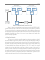
The new system adopts the “thin-client and fat server” architecture with three basic tiers of Web
application: presentation tier, logic tier, and data tier, as shown in Figure 4-2. The presentation
tier includes the user interface terminal through which users interact with the application. The
logic tier, which is also called the computational tier, is the core component of the DRIVE Net
system. It performs computations to assist in customized analysis and decision making based on
users’ interactive input. The data tier organizes and supports data requested for analysis.
Normally the client handles the user interface while the server is responsible for the data. The
significant difference between “thin-client and fat server” and “fat-client and thin server” is the
shifted responsibility for the logic/computational tier (Lewandowski, 1998). In fat server
systems, the server fully takes over the logic/computation tier while the client only hosts the
presentation tier for displaying the user interface and dealing with user interactions.
There are three reasons to adopt the thin-client architecture: First, no plug-in and
installation are required at the client side except a basic browser, which ensures the highest level
of compatibility. Given that the system is designed for customers with constrained network
functions, minimal requirements on the client side are most desirable. Second, there are fewer
security concerns since all the data and computational tasks are manipulated and performed on
the server side, and the client is only responsible for user interaction and results presentation.
Third, mature frameworks for building thin client Web applications could be re-used to boost
development productivity. However, thin-client architecture does have its drawbacks. One major
disadvantage is that the performance of the system depends solely on the server and, as a result,
excessive user requests greatly affect system efficiency. This has become more manageable in
recent years with the continuous advancement of cloud computing technologies such as Amazon
Web Service, whose the cloud servers are fully designed to improve system performance.
Page 23
Client Side
HTTP(S)
OpenStreetMap Server
Web Mapping Service
DRIVENet Web Server
R Server
Statistical Analysis Service
Real‐time Traffic
Incident Induced Delay Calculation
Dynamic Routing
Travel Time Performance Measure Pedestrian Trajectory Reconstruction
Freight Performance Measure
Traffic Emission Evaluation
Corridor Sensor Comparison Freeway Performance Measure Server Side
OpenStreetMap
WSDOT Roadway Geometric data
Loop Detectors
Data fusion
Data fusion
Data fusion
Weather
Geospatial Data Transportation Data
HPMS
INRIX Speed
…...
…...
TMC Network
WITS
Data Quality Control
…...
File Importing
FTP Downloading
Data Sources
Data Sources
External Database Connecting
…...
Data Sources
Figure 4-2 DRIVE Net 3.0 Architecture
Page 24
The data communication flows in the DRIVE Net system can be summarized as follows:
1.
The end-user sends an HTTP(S) request to the Web server.
2. The Web server looks into the request and retrieves the related data information
from the data warehouse.
3. The warehouse sends back the requested data and the Web server performs the
computational tasks by using either the built-in analytical tools or external statistical
modules provided by R Server.
4. If geospatial analysis is involved, the Web server connects to the OpenStreetMap
Server and requests the map.
5. Analysis results as well as the map are then returned to the client. The Web browser
displays the results or visualizes the returned objects on the map.
4.3 System Implementation
As mentioned in the previous section, the DRIVE Net architecture has been redesigned to meet
challenges. To reduce costs and boost productivity, multiple open source products are utilized.
Relying on open source products, the DRIVE Net team not only takes advantages of codesharing and collaboration with a broad community of developers but also contributes to open
source projects. The core open source products combined into the DRIVE Net system are
explained in the remainder of this section.
4.3.1 OpenStreetMap and OpenLayers
OpenStreetMap (OSM) is a collaborative project that has created a comprehensive worldwide
map that is free to use and editable (Haklay et al., 2008). With the outlook that geospatial data
should be freely accessible to the public, University College London established the OSM
project in July 2004, and it is one of the most prominent and famous examples of Volunteered
Geographic Information, a concept introduced by Goodchild (2007, 2008). The process of
maintaining OSM data is termed crowdsourcing and is being used by a number of other
commercial companies such as Google and TomTom. In crowdsourcing, a term defined by
Brabham as an “online and distributed problem-solving and production model,” labor-intensive
tasks are distributed to large groups of users, and this has allowed volunteers to create and update
geospatial data on the Internet. By January 2013, OSM had over one million registered
contributors and 20,000 active users worldwide, and the number continues to rise dramatically
(Wood, 2013). Besides governments, OSM has obtained strong support from commercial
Page 25
companies. For instance, Yahoo Maps made its vertical aerial imagery available to OSM as a
backdrop for map production in 2006, and Microsoft Bing Maps donated part of its satellite
imagery to the OSM in 2010 (Microsoft, 2010).
One major reason for DRIVE Net to choose OSM is its low cost in comparison to
commercial datasets, as well as its data sharing nature. With the Open Data Commons Open
Database License (ODbL), developers are free to use, distribute, and modify the OSM data as
long as OSM and its contributors are credited (OpenStreetMap, 2013). Using OSM to replace
Google Maps helps DRIVE Net avoid potential charges by Google, Inc in the future that might
eventually prevent the project from growing. In addition, in keeping with the theme of eScience,
the DRIVE Net developers prefer open source products over commercial ones because they can
help share ideas, drive innovation, and boost productivity for the entire community.
High-resolution and qualitative geographic information such as that shown in Figure 4-3
makes OSM an appealing replacement for Google Maps. Recent research confirms the good
quality of OSM and its ability to compete against commercial geodata, especially for urban
areas. Zielstra and Hochmair (2011) used the commercial datasets NAVTEQ and TeleAtlas, as
well as the freely available dataset TIGER/Line, to quantify the coverage of OSM in the United
States. The results indicated that “there is strong heterogeneity of OpenStreetMap data for the
U.S., in terms of its completeness,” A similar study was done in Germany by Zielstra and Zipf in
2010 (Zielstra et al., 2010). The paper states that some projects already replaced proprietary data
with rich OSM data in larger cities. In the U.K., Haklay (2010) performed a comparison with the
Ordinance Survey (OS) Meridian dataset by evaluating the accuracy, completeness, and
consistency of the positions and attributes. The analysis concluded that “OSM information can
be fairly accurate,” with a positional accuracy of about 6 meters and an approximately 80 percent
overlap of motorway objects in comparison to the OS dataset.
Page 26
Figure 4-3 High Resolution OpenStreetMap near the University of Washington
Figure 4-4 shows how clients dynamically interact with OpenStreetMap in the DRIVE
Net system and the backend processes. When a Web server receives clients’ request for a map, it
transmits the request to the OSM mapping server for retrieving map contents. The OSM mapping
server renders the map with specified geospatial information and sends it back to the Web server.
The Web server then passes the map contents to clients. On the client side, OpenLayers provides
the service to obtain map images from servers and display map tiles on the screen (Haklay et al.,
2008). OpenLayers is an open-source JavaScript library running on the client side that helps
users interact with dynamic maps from disparate services. A number of extra features are
provided by OpenLayers. Specifically, it allows developers to lay numerous data on top of map
layers, such as vector layers, markers, and pop-up windows, as Figure 4-5 demonstrates.
Server Side
Page 27
Web Server
OSM Server
OpenStreetMap Database
Client Side
OpenLayers
Request map
Receive map
Direct Download
Clients
Figure 4-4 Communication Mechanism for OpenStreetMap
Page 28
Figure 4-5 Multiple Layers on Top of a Map
4.3.2 R and Rserve
R is a free and powerful statistical analysis tool utilized by more than two million people for
machine learning, statistical modeling, and data visualizations (R, 2013). With thousands of
active contributors from academia, R keeps evolving with the latest efficient and innovative
algorithms. Meanwhile, R provides excellent tools for creating graphics, which enable users to
gain better insights via data visualization. Rserve, a TCP/IP server connecting to R, integrates R
into the DRIVE Net system so that it takes full advantages of R’s statistical computation
capability (Rserve, 2013). Several modules in the system use the combination of Rserve and R as
the major tool for statistical analysis and data visualization, as Figure 4-6 demonstrates. By
integrating R and its countless statistical and graphic packages, DRIVE Net offers an easy and
Page 29
customizable interface for performing complex analysis and data visualization for users, even
those without any background knowledge of R scripts.
Figure 4-6 Travel Time Performance Measurement
Page 30
Chapter 5 HCM 2010 Freeway Performance Monitoring
To demonstrate the data sharing, integration, visualization, and analysis capabilities of the
DRIVE Net eScience transportation platform, a pilot research effort on automating networkwide, real-time freeway performance measurement was undertaken. It is described in this
chapter.
5.1 Background
Real-time freeway performance measurement helps quantitatively describe traffic conditions to
transportation researchers, operators, planners, and the general public in a timely manner. With
network-wide, real-time information, decision makers can not only quickly evaluate the quality
of service on transportation facilities and identify congestion bottlenecks, but can also promptly
coordinate facility management and refine policy and investment decisions. The ultimate goal of
measuring freeway performance is to improve transportation mobility and accessibility.
The most widely used guidance for measuring freeway performance is the HCM 2010,
which has been undergoing constant revision since 1944 (Kittelson, 2000). The 2010 HCM,
published by the Transportation Research Board of the National Academies of Science, is a
collection of state-of-the-art methodologies for quantifying the quality of service on
transportation facilities. One important concept introduced by the HCM is level of service
(LOS), which represents a qualitative ranking of traffic performance ranging from A to F. LOS
A represents the best traffic operational condition, while F is the worst. In this study the HCM
2010 methods were applied to quantify freeway performance. Although every DOT collects realtime traffic data as well as roadway geometric data, there is no universal procedure for utilizing
available datasets and automating network-wide freeway operational analysis. FREEVAL 2010,
a computational engine executed in Microsoft Excel, is one alternative for freeway facilities
analysis (HCM, 2010). However, FREEVAL requires users to manually input geometric and
traffic demand information for each segment, which can be extremely cumbersome when
analyzing long roadway segments across multiple periods. With DRIVE Net’s significant
computational power and comprehensive data (such as mainline loop detector data, freeway
geometric factors, INRIX speed, etc.), it provides a mature platform from which to perform realtime LOS analysis for freeway segments. Because of the limited information on ramp geometry,
Page 31
on-ramp volumes, off-ramp volumes, and weaving volumes, this study focuses only on
quantifying traffic operational performance for basic freeway segments.
5.2 Challenge
The methodology in HCM 2010 has limitations. First, HCM methods can be applied to local
oversaturated conditions, but not when system-wide oversaturation occurs. Second, some special
conditions are not taken into account, such as road segments near toll plazas, free-flow speed
above 75 mph, or free-flow speeds below 55 mph. Although the HCM recommends potential
alternative tools to fill these gaps, most of them are commercial simulation tools. Given the cost
and technical challenges, it is not an ideal solution to perform such real-time analyses in DRIVE
Net.
Measuring network-wide performance poses challenges for integrating multiple
geospatial data layers. Different GIS data layers have different line segments, even when they
share the same route, start point, and end point. For example, in Figure 5-1, the same route on I-5
northbound from milepost 0 to milepost 10 is segmented into different lines in different GIS data
layers. One possible solution is to use a line-to-line vector overlay, as Figure 5-2 shows.
However, the operation of a network-wide multi-layer overlay on the fly is inefficient and timeconsuming. Better spatial data fusion techniques are needed to efficiently and accurately
integrate multiple geo-data sources.
Page 32
Figure 5-1 Geospatial Data Fusion Challenge
Figure 5-2 Vector Overlay
The objective of this case study was to automate freeway performance measurement in a
consistent, efficient, and accurate manner, given existing resources that included geometric
factors, loop detector data, and INRIX speed data. The DRIVE Net platform was utilized to
Page 33
implement the automation, not only because of its interoperable data framework but also because
of its customizable computing power. The rest of this chapter elaborates on the spatial modeling
framework for network-wide freeway performance measurement.
5.3 Modeling Framework
The modeling process was divided into two main phases, as shown in Figure 5-3. In the first
stage, the roadway network was segmented by using an innovative spatial data fusion technique
called pixel-based segmentation. Once the segmented network had been formed, three different
methods were applied to compute LOS in phase 2, namely, the HCM 2010 Method, HCM 2010
Method with INRIX Speed Data, and Multi-regime Prediction Method.
Phase1:SegmentRoadwayNetwork&Integrate
GISLayers Pixel‐basedSegmentation
DetermineFFS
Inputvolumes
Loop
Detector
Data
INRIXSpeed
Input historical speed data sets
Input real‐time INRIX Speed
AdjustDemand
Volume
Input historical adjusted demand volume
Inputhistorical
data
Input real‐time demand volume
Inputreal‐time
data
CalculateDensity&
DetermineLOS
CalculateDensity&
DetermineLOS
FinalizeLOS
Multi‐Regime
Regression
PredictLOS
Figure 5-3 HCM2010 Modeling Framework
Page 34
5.3.1 Segment Roadway Network and Integrate GIS Layers
With heterogeneous datasets, multi-layer geospatial data processing is necessary in order to
superimpose multiple GIS layers to generate an output layer. To calculate performance
measurements, a fundamental network layer has to be prepared, in which each basic roadway
segment has the same attribute data as input value. In particular, the HCM 2010 requires the
roadway to be segmented uniformly. Uniform segments must share the same attribute data,
including geometric features and traffic features. In GIS, vector overlay is the common and
major solution for combining both the geographic data and attribute data from multiple input GIS
layers, as presented in Figure 5-2. However, in our case, the network-wide large volume spatial
data made the overlay analysis time consuming and computationally intensive. Additionally, if a
new GIS layer was imported into the DRIVE Net data warehouse, it would not be realistic to reperform the entire series of overlay operations.
Therefore, pixel-based segmentation, a novel method for modeling the geospatial data,
was proposed. It borrows from the concept of pixels in digital imaging. A pixel is generally
treated as the fundamental unit of a digital photo, extracted from the words “PICture ELement”
(Wikipedia, 2013). In a digital image, millions of pixels are combined together to resemble the
subject of the image. The quality of the image greatly depends on the total number of pixels
used, which is defined as resolution. As Figure 5-4 illustrates, the more pixels an image contains,
the more details it is able to reveal.
Figure 5-4 Image Resolution (Wikipedia, 2013)
Similarly, pixel-based segmentation subdivides a roadway network into basic segments
of equal length, called line pixels. The length of a line pixel defines the resolution of the
segmentation. The shorter the pixel length is, the more details the output network contains. For
instance, in Table 5-1, I-5 northbound with start milepost 140.4 and end milepost 140.9 is
subdivided into five basic segments of equal length (0.1 mile each). The output network attribute
data use the combination of route ID, start milepost, and end milepost as a unique key to link
Page 35
with the geographic data. With the geographic data already segmented into equal line pixels, the
process of superimposing multiple GIS layers can be accomplished with the attribute data only.
Because the Linear Referencing System (LRS) that WSDOT has adopted to identify the
locations of features is based on state route ID and feature distance in miles from route beginning
(WSDOT’s Linear Referencing System, 2013), it is easy and fast to retrieve corresponding
features given the route ID, start milepost, and end milepost.
Table 5-1 Examples of Segmented I-5
Urban
Rural
Terrain
TRD
Lanes
Avg
width
Upper
Ramp
MP
Lower
Ramp
MP
48
4
12
U
Level
0.8333
141.64
138.04
10
48
4
12
U
Level
0.8333
141.64
138.04
North
10
48
4
12
U
Level
1
141.64
138.04
140.8
North
10
48
4
12
U
Level
1.1666
141.64
138.04
140.9
North
10
48
4
12
U
Level
1.1666
141.64
138.04
Should
er
width
Rdwy
width
North
10
140.6
North
140.6
140.7
5
140.7
5
140.8
Start
MP
End
MP
DIR
5
140.4
140.5
5
140.5
5
Route
Num
Pseudo code for integrating attribute data from multiple GIS layers can be found below:
function integrateGISLayers
for each route r in network
for k = 0; k < r.length; k = k + pixel_length
start_mp = k;
end_mp = k + pixel_length;
for each input GIS Layers l
# look up attribute data of l
# given routeid, start_mp and end_mp
outputLayer[r, start_mp, end_mp, l]
= getAttributeDate(I, r, start_mp, end_mp);
end
end
end
output outputLayer;
The pixel-based segmentation was used in this study for the following reasons: First, it
separates the attribute data from geographic data. In comparison to vector overlay operations, the
integration of attribute data based on LSR is more efficient, fast, and easy to implement. Second,
the fixed segmentation will make it convenient to integrate more GIS layers into an existing
network in the future, as long as the pixel resolution remain the same. Third, the value of pixel
Page 36
resolution is flexible, which allows us to select the level of accuracy to achieve. If the line pixel
is infinitely close to 0, the output attribute table will capture perfect details no matter how many
GIS layers are imported. In reality, pixel size 0.1 mile is a good choice for balancing efficiency
and accuracy.
5.3.2 Calculate LOS using the HCM 2010 methodology
Because of limitations in available datasets, this study focused only on LOS calculations for
basic freeway segments. The HCM 2010 provides a comprehensive method for analyzing LOS,
as shown in Figure 5-3, Phase 2.1. Notice that no measured free flow speed (FFS) was available
for the entire network layer; rather, FFS was computed by lane width adjustment and lateral
clearance adjustment in this study. The HCM 2010 is unable to handle system-wide
oversaturated flow conditions, and focuses only on analyzing under-saturated flow conditions.
Over-saturated flow conditions are discussed in the next section.
Step 1: Input Data
In this step, demand volume, number and width of lanes, right-side lateral clearance, total ramp
density, percentage of heavy vehicles, peak hour factor, terrain, and the drive population factors
are retrieved from the DRIVE Net data warehouse.
Demand Volume
Real-time demand volumes are mainly estimated from loop detectors. The system automatically
fetches all the cabinets between the Nearest Upstream Ramp (NUR) and the Nearest
Downstream Ramp (NDR), and then it queries the corresponding latest 15-minute flow. Demand
volume is calculated by using the following equation:
4
:
15
|
(5-1)
/
The median is selected to measure the central tendency, since it naturally eliminates the
outliers. It is then multiplied by 4, which projects into hourly volume. For instance, in Figure 55, there are six cabinets between the upstream and downstream ramps. The 15-minute flows
fetched are shown as 500, 100, 450, 450, and 550. Hence, hourly volume for the segments
between the upstream and downstream ramps is equal to 450×4=1800 veh/h. Notice that if no
cabinets/loop are detectors between the upstream and downstream ramps, the system will assume
Page 37
that there is no demand volume input for segments and will use real-time INRIX speed and a
historical regression model to predict LOS, which will be discussed later in this chapter.
Figure 5-5 Nearest Upstream and Downstream Ramps
Total Ramp Density (TRD)
Total ramp density (TRD) is defined as the total number of ramps (both on and off with one
direction) within 2 miles of the midpoint of the segment under study. Given the study segment
start milepost and end milepost, the following equation could be used to calculate TRD:
Page 38
2
│
3
3 /6
(5-2)
Other Input Data
The geometric data, including number and width of lanes, right-side lateral clearance, and
terrain, are originally downloaded from the WSDOT Roadway Datamart for GIS (Roadway
Datamart, 2013). Geospatial data fusion is performed by using the methods introduced in the
previous section. Because no site-specific data are available for the remaining features, default
values recommended by NCHRP Report 599 (Zegeer et al., 2008) are used.
Table 5-2 Default Values for Basic Freeway Segments
Required Data
Peak Hour Factor
Driver Population Factor
Percentage of heavy vehicles (%)
Default Values
Urban: 0.92, Rural: 0.88
Urban: 1.0, Rural: 0.975
Urban: 5%, Rural: 12%
Step 2: Determine Free-Flow Speed
Because the site-specific measured FFS is not available, the following equation,
developed by HCM 2010, is used to estimate FFS. Lane width, right-shoulder lateral clearance,
and ramp density are taken into account to adjust the Base Free-Flow Speed (BFFS). The
estimated FFS is then rounded to the nearest 5 mph as HCM suggests. The adjustment value can
be found in HCM 2010.
.
3.22
75.4
where
Step 3: Adjust Demand Volume
(5-3)
Page 39
Demand volume obtained from loop detectors must be converted into service flow rate under
equivalent base conditions. According to the HCM 2010, the base conditions for a basic freeway
segment are specified as follows:

12-ft lane widths

6-ft right shoulder clearance

100 percent passenger cars in the traffic stream

level terrain.
A driver population of regular users familiar with the roadway is then used for the
conversion:
(5-4)
where
/ /
/
The heavy-vehicle adjustment factor can be calculated by the following equation:
(5-5)
where
Page 40
As HCM suggests, the proportion of recreational vehicles in the traffic stream is small and close
to 0 in many cases. Hence, in this study,
passenger car equivalent factors
and
was set to be 0 as the default value. The value of
are also recommended by HCM 2010 on the basis of
the type of terrain or grades.
Step 4: Calculate Density and Determine LOS
Given the FFS from Step 2 and adjusted volume
from Step 3, the average passenger car
speed S can be found in Figure 5-6 or computed by the speed-flow equation in Table 5-3. Then
the density
can be derived:
(5-6)
Once the density has been computed, the LOS
can be determined from Table 5-4.
Figure 5-6 HCM Speed-Flow Model (HCM, 2010)
Page 41
Table 5-3 Speed-Flow Equations (HCM, 2010)
Table 5-4 LOS Criteria for Basic Freeway Segments
Density
11
18
26
35
45
LOS
A
B
C
D
E
5.3.3 Incorporate the Real-Time INRIX Speed into LOS Calculation
One of the limitations of the HCM method is that it cannot analyze system-wide oversaturated
conditions. In other words, once the demand is greater than the capacity, HCM is unable to
estimate space mean speed as well as density. However, in reality, it is critical to identify
oversaturated conditions spatially and temporally so that operators and planners can understand
bottlenecks (formation, propagation, and dissipation) in their facilities. As suggested by Figure
5-7, in oversaturated conditions traffic speeds drop dramatically, typically below 35 mph. To fill
the gap of analyzing oversaturated conditions, INRIX speed data are incorporated into the LOS
calculation. With the demand volume still obtained from loop detectors and adjusted by the
HCM 2010 methodology, INRIX speed
is used to estimate the density as shown below:
1 0 45
45
Page 42
∙
1
∙
(5-7)
where
/ /
Additionally, using INRIX speed to estimate LOS provides ground-truth data by which to
judge the feasibility of HCM methodologies, as discussed in section 5.4.
Figure 5-7 Undersaturated, Queue Discharge, and Oversaturated Flow (HCM, 2010)
5.3.3 Develop Empirical Speed-Density Regression Equations to Predict LOS
The quality of traffic data greatly influences the accuracy of performance estimation and as
among the primary concerns in this analysis. Data quality issues involve at least (1) missing data,
(2) suspicious or erroneous data, and (3) inaccurate data (Turner, 2001). Erroneous data are those
that do not follow accepted principles or go beyond thresholds, while inaccurate data contain
inexact values due to measurement error. In this study, these three types of errors were all treated
Page 43
as invalid traffic data entries. The data quality issues involved two major challenges: (1) how to
identify the bad data and (2) how to compensate for the invalid data input.
Many efforts have been made to develop comprehensive and sophisticated data quality
checking methods. In practice, the threshold approach is often adopted to ensure that sensor
values fall within a reasonable range. The combination of volumes, speed, and occupancies
provides a relatively straightforward yet robust way to check data error. Jacobson et al. (1990)
developed an algorithm that uses volume-to-occupancy ratios to examine the reliability of loop
detector data. In addition, time series of traffic samples can be used for comparison. For
example, Chen et al. (2003) proposed a diagnostics algorithm to efficiently find malfunctioning
single-loop detectors on the basis of the sequence of volume and occupancy measurements for an
entire day. Ishak (2003) developed a fuzzy-clustering approach to measure uncertainties in
freeway loop detector data. Moreover, measuring spatial relationships between detectors also
turns out to be an effective tool for accurately detecting errors. Kwon et al. (2004), for instance,
utilized the strong measurement correlations between upstream and downstream sensors to detect
spatial configuration errors.
All those advanced algorithms demonstrate robust solutions in identifying quality issues
related to loop detectors. A related question is how to estimate real-time density or LOS when
the input demand volume is invalid. With the relatively comprehensive speed dataset from
INRIX, this research focused on predicting real-time density, given historical traffic data and
real-time speed, as the solution to dealing with invalid input volume.
Empirical speed-density relationships provide the most abundant source of data for
performing predictions. Over the past few decades, a great deal of research has been done on
developing speed-density models. Because of its data-driven nature, a multi-regime model based
on cluster analysis (Sun et al., 2005) was adopted to fit empirical speed-density observations.
This method first applies a K-means algorithm to traffic datasets, which naturally partitions the
data into homogenous groups. It then applies a series of single-regime models to find the one that
best fits the data, such that breakpoints can be automatically determined. Notice that Sun’s
method chooses the k value by trial and error; in this study, the optimal number of clusters was
determined by the average Silhouette criterion instead of trial and error. For conceptual testing
Page 44
purposes, only linear, logarithmic, and exponential models were included. Pseudo code for
building a multi-regime traffic model can be found below:
function PerformSpeedDensityRegression
# Given traffic datasets observations
# Choosing k using the Sihouette
k = DetermineKbySihouette(observations);
clusters = kmeans(observations, k);
for each cluster c in clusters
# three basic functions chosen to fit c
lmReg = lm(c.speed ~ c.density, data = c);
logReg = lm(c.speed ~ ln(c.density), data = c);
expReg = lm(c.speed ~ exp(c.density), data = c);
#choose the regression model fits best
bestReg = max(lmReg.Rsquare, logReg.Rsqaure, expReg.Rsquare);
output bestReg;
end
5.4 Implementation Result
The aforementioned modeling framework was implemented in a real-world network for pilot
testing purposes. The I-5 northbound corridor in Seattle, Washington, from milepost 140 to
milepost 195 was selected as the study site. It is the primary travel route connecting Tacoma and
Everett through downtown Seattle, and it has the most comprehensive traffic data available.
Figure 5-8 shows cabinets 140 deployed by WSDOT along the corridor. In the next several
subsections, network segmentation and data preprocessing are briefly introduced, followed by an
explanation of LOS results computed from the three proposed methods: the HCM 2010 method,
the HCM 2010 method with INRIX speed data, and the multi-regime regression method. The
satisfactory results further confirm the reliability and feasibility of the proposed modeling
framework.
Page 45
Figure 5-8 I-5 Northbound Corridor (Tacoma - Everett)
5.4.1 Network Segmentation
By applying pixel-based segmentation to the geographic data, introduced in section 5.3, the
corridor was subdivided into 550 basic freeway segments with pixel length of 0.1 mile. The
corresponding attribute data were then fused according to route ID (I-5), start milepost, and end
milepost. Table 5-5 presents the sample attribute data. Notice that the roadway geometric data
Page 46
are relatively static and not updated very often. It is more efficient and effective to pre-process
the attribute data fusion instead of running it on the fly.
Table 5-5 Fused Attribute Data
Route
Start
MP
End
MP
DIR
5
140.4
140.5
North
Should
er
width
10
5
140.5
140.6
North
10
5
140.6
140.7
North
5
140.7
140.8
5
140.8
140.9
0.8333
Upper
Ramp
MP
141.64
Lower
Ramp
MP
138.04
0.8333
141.64
138.04
Level
1
141.64
138.04
U
Level
1.1666
141.64
138.04
U
Level
1.1666
141.64
138.04
Rdwy
width
Num
Lns
Avg
width
Urban
Rural
Terrain
TRD
48
4
12
U
Level
48
4
12
U
Level
10
48
4
12
U
North
10
48
4
12
North
10
48
4
12
5.4.2 Volume and Speed Data Sets
Real-time volume data are collected from single loop detectors every 20 seconds, and INRIX
speed data are aggregated every 1 minute on the basis of GPS data, respectively. Both datasets
are archived in the DRIVE Net database. For pilot testing purposes, two-day observations were
extracted and utilized in the latter computation. The two traffic datasets were further aggregated
into 15-minute time intervals, as recommended by the HCM. Data quality control techniques
were applied to ensure data accuracy. For example, several thresholds were set to eliminate
obvious outliers. Comprehensive data quality control is critical to the DRIVE Net system. For
more detail, please refer to (Wang et. al., 2009).
Figure 5-9 shows the scatter plot of adjusted volume
density,
volume,
vs. speed
vs. speed
as well as
, for a total of 95,040 observations. Notice that the service
, used in Figure 5-9 was under base conditions, converted from real-time traffic
counts following the HCM 2010 methods.
Page 47
Figure 5-9 INRIX Speed, Adjusted Volume, and Density
5.4.3 HCM Method with/without INRX Speed Data
The HCM method with volume only and HCM method with volume and speed were applied to
compute
and
, respectively. Because the HCM method is unable to analyze
oversaturated conditions (LOS = F), the comparison between
and
was conducted for
undersaturated flow only. Of the total 92,400 observations that fell into the undersaturated
conditions, 83.83 percent of
was equivalent to
, a total of 77,458 data points. The
match rate increased to 98.98 percent if adjacent LOS’s were treated as approximately equal
(e.g., LOS A≅LOS B). The fact that these two methods were highly consistent in estimating
LOS delivers suggests the following: (1) the proposed methodologies such as pixel-based
segmentation can generate satisfactory accuracy; (2) using INRIX speed data to determine
oversaturated conditions is feasible and cost effective; and (3) the quality of INRIX speed data is
proved to some extent, given the consistency between results computed with both HCM methods
in Phase 2.1 (without INRIX speed data) and Phase 2.2 (with INRIX speed data).
Page 48
Table 5-6 and Figure 5-10 compare the LOS category counts produced by the two
methods. Note that LOS computed by using INRIX speed usually underestimated service quality.
These results are consistent with recent research on transportation sensor comparisons conducted
by Dr. Yegor Malinovskiy from the UW STAR Lab, who found that INRIX speed data usually
have a smaller standard deviation and tend to underrate traffic conditions.
Table 5-6 LOC Count by Phase 2.1 (without INRIX Speed Data) and Phase 2.2 (with
INRIX Speed Data)
LOS
A
B
C
D
E
F
HCM Method
37430
30343
18677
5756
194
2640
HCM Method with INRIX Speed
35994
25188
20324
8077
2817
2640
Page 49
Figure 5-10 LOS by Phase 2.1 (without INRIX Speed Data) and Phase 2.2 (with INRIX
Speed Data)
5.4.4 Regression Analysis
To compensate for missing or low quality data, an empirical multi-regime density-speed model
was used to predict density in this study. During the implementation, the two-day datasets were
divided evenly into a training set (November 07, 2011) and a testing set (November 08, 2011) to
avoid overfitting to test conditions.
Page 50
function PerformSpeedDensityRegression
# Given traffic datasets observations
# Choosing K using the SilHouette
K = DetermineKbySilhouette(observations);
clusters = kmeans(observations, K);
for each cluster c in clusters
# three basic functions chosen to fit c
lmReg = lm(c.speed ~ c.density, data = c);
logReg = lm(c.speed ~ ln(c.density), data = c);
expReg = lm(c.speed ~ exp(c.density), data = c);
#choose the regression model fits best
bestReg = max(lmReg.Rsquare, logReg.Rsqaure, expReg.Rsquare);
output bestReg;
end
Following the procedures described in the pseudo code above, the K value was chosen to
be 2 by using the Silhouette. According to suggestions from Sun et al. (2005), using the original
data for the K-mean algorithm would outperform the normalized data. Hence, this study applied
the K-mean algorithm to the training set without normalization. The clustering results can be
found in Figure 5-11 and Table 5-7. As expected, Cluster 1 had high speed and low density,
which represents a free-flow regime, while Cluster 2 had lower speed and high density, which
represents congested-flow regime.
Three single-regime models, namely, linear, logarithmic, and exponential functions, were
then used to fit Cluster 1 and Cluster 2, respectively. The one with the greatest R squared value
was chosen to represent the empirical speed-density relationship. The following equation shows
the final two-regime model obtained from the training set:
66.3237
exp 4.657
0.1851 0.02169
24.6
24.6
(5-8)
Page 51
Figure 5-11 Training Set: Two Clusters by K-means Algorithm Analysis
Table 5-7 Training Set: Clustering Centers by K-means Algorithm
I-5 Northbound
Speed (mile/h)
Density (pc/mile)
Percentage
63
16.94186
80.27%
53
32.87736
19.73%
As Figure 5-11 shows, the two-regime model fit the training set quite well. A comparison
between the ground-truth value
and predicted value
for both training set and testing
set was further conducted. The testing set yielded an even lower error, as indicated in Table 5-8.
If adjacent levels were treated as approximately equal, both training error and test error were less
than 5 percent (shown as an accuracy of
1in Table 5-8). This proves the feasibility and
accuracy of the proposed modeling framework.
Page 52
Table 5-8 Test Results
Date Set
Training Set
Test Set
Accuracy
57.7%
59.84%
Accuracy of
95.38%
95.01%
1
5.4.5 Data Visualization
Figure 5-12 shows the user interface designed for the freeway performance measurement
module. The control panel is located on the left side, while the interactive map is on the right.
Users are free to input date, time, route ID, route direction, start milepost, and end milepost and
to query the corresponding LOS map by clicking the button “LOS Map”. As long as the system
receives the user request, it will show the LOS map based on criteria described in the color
legend on the left. As Figure 5-13 shows, the LOS map gives a straightforward way to
demonstrate LOS spatially, which enables users to easily identify bottlenecks. Additionally, a
related statistics report can be prepared and automatically displayed for downloading if users
click the button “Statistics Report”. The report includes detailed information such as segments,
geometric factors, speed, density, and LOS, which enables users to further analyze the data.
Figure 5-122 User Interface Design
Page 53
Figure 5-133 Data Visualization: LOS Map
Page 54
Chapter 6 Computational Methods for WSDOT Gray Notebook
(GNB) Statistics Calculation
As a primary accountability reporting tool, WSDOT’s Gray Notebook has been updated
quarterly and annually since 2001. The report summarizes multiple aspects of the Washington
state transportation system, including safety, rest areas, ferry vessel and terminal preservation,
travel information, wetlands protection, commercial vehicle information systems and networks,
and trucks, goods and freight (WSDOT, 2013). To better monitor and alleviate congestion,
WSDOT also publishes its congestion report annually. The Department utilizes various detectors
to collect transportation data, which are then analyzed for reporting purposes. Such congestion
reporting assists the public and WSDOT officials in gaining a better understanding of whether its
existing congestion mitigation countermeasures are effective (WSDOT, 2012). The statistics
generated from the congestion report are incorporated into the WSDOT Gray Notebook.
Traditionally, processing massive transportation data and calculating congestion
measures are labor-intensive tasks that require intensive efforts to coordinate among different
partners. In addition, the complexity of congestion analysis requires the expertise of various
disciplines, so WSDOT has to spend a great deal of manpower and time to produce the
congestion report each year. However, the DRIVE Net system can address these issues by
integrating multiple data sources, conducting desired analytical functions, and presenting the
congestion report via a map-based, online platform.
This chapter describes how the loop detector data are first preprocessed through a
comprehensive data quality control procedure to detect, remedy, and correct erroneous records.
Next, the processed data are further incorporated into a computational engine for Gray Notebook
statistics calculation. The generated performance indicators are then visualized by the DRIVE
Net system and used to generate all the necessary reporting and graphic functions required by
WSDOT.
6.1 Freeway Loop Data Quality Control
Data quality control (DQC) was a key component in this research because quality data yield
reliable information on which smart decision making depends. Early DQC work, such as that
Page 55
conducted by Ingram (1976) and Chen and May (1987), focused on raw inductive loop detector
output. Specifically, detector level errors include chatter (rapid cycling of the detector), crosstalk
(adjacent sensors actuating together), and failed on/off sensors, among others. Over time, many
of these early, detector-level diagnostics have been incorporated into the detectors themselves,
controller software, and practice. It is important to remember that these basic diagnostics, while
well-known and accepted for loop detectors, may apply to other detectors that do not have the
history of inductive loop detectors. For the next level of DQC, blocks of data from a sensor are
used to determine whether the results it presents are within expected boundaries. A number of
such threshold methods were developed during the 1990s. Good summaries of these methods
were compiled by Turochy and Smith (2000) and May et al. (2004). Threshold-based methods
can be thought of as drawing lines on a chart and discarding data that lie beyond the lines. For
example, a maximum volume threshold would discard data that reported volumes greater than
the threshold maximum value. Current DQC research has two branches: the first uses network
information to identify errors and the second has returned to the event roots used in earlier
research. Network-based DQC methods focus on volume correction, typically relying on
conservation of vehicles between sensor stations, as in the work done by Wall and Dailey (2003).
Loop detector data are used to compute Gray Notebook statistics. A two-step data quality
control procedure is proposed: first, the raw loop data should be subjected to a series of error
detection tests to identify missing and erroneous data. These data should then be flagged for
further corrections and remedies. Several statistical algorithms were developed to estimate the
missing data and replace those erroneous records. The corrected data should be periodically
stored in the database for Gray Notebook calculation. The 20-second loop data and 5-minute data
should all be processed for quality control purposes.
Page 56
Data Error Detection
Data Error Correction
Basic Thresholding
Checking
Controller‐
based Checking
Spatial Correction
Temporal Correction
Raw Loop Data
Sensitivity Checking
Health Score Calculation
Archived Loop Data
Gaussian Mixture Model
Update
Processed Loop Data
Figure 6-1 Loop Data Quality Control Flow Chart
Figure 6-1 shows how incoming loop detector data are processed in the DRIVE Net DQC
procedure. Shortly after the raw data arrive, the first data quality control checks are performed.
The research team found it very important to maintain the raw data in addition to the processed
data. Keeping the original raw data allowed the research team to improve the data quality control
algorithms and quantify their efficacy. It also served as an insurance policy against false
positives in the DQC algorithms.
6.1.1 Data Error Detection
The first step is to utilize the controller-equipped error detection mechanism to identify
data errors. WSDOT’s loop detector cabinets are able to provide simple data quality checking on
the hardware end, and to flag errors directly with each record. These errors include short pulses,
loop chatter, and values outside of allowable volume/occupancy ranges, and they include a flag
for operator-disabled loops (Ishimaru and Hallenbeck, 1999). To be specific, the existing
columns in the raw loop data include several flags to indicate the status of each record. For
instance, the “Data” column in the 20-second loop database is an indicator of missing data. This
data quality control procedure focuses on daily loop data for preliminary checking. If more than
90 percent of the records for a particular loop detector are considered to be “good data” by the
controller, then this loop can be used for freeway performance monitoring.
Page 57
The raw loop data are then further transferred to a series of error detection procedures.
The simplest approaches are the threshold-based methods. They are designed to check whether
the incoming data are valid and within expected bounds. This is an important step because some
sensors feeding the DRIVE Net system report -1 for the volume as an error flag, which can cause
calculation errors if this value is not corrected and converted into a bad data flag. These
threshold criteria are listed below according to Chen et al. (2003):
a. For each time interval, the volume is zero while the occupancy is greater than zero.
b. For each time interval, both volume and occupancy are zero (between 5:00 AM and
8:00 PM).
c. For each time interval, the occupancy exceeds 0.35.
The loop data samples are retrieved from 5:00 AM to 8:00 PM, as it is hard to judge the
loop data quality beyond this time range using the above three criteria. For a given day, there are
3240 20-second records and 216 5-minute records per detector. For each loop detector, the
number of records belonging to error type (a), (b), and (c) are denoted as Na , Nb , Nc
respectively, and the criteria to check the status of a loop detector for any date are expressed as:

0
flag  
1
Na
N
N
 pa , b  pb , c  pc
N
N
N
otherwise
if
(6-1)
where N is the number of time intervals of daily loop data (3240 for 20-second loop data and
216 for 5-minute loop data), and pi (i  a, b, c) is the percentage threshold belonging to error
type a, b, or c.
The above DQC procedures have inherent shortcomings for detecting systematic errors
such as over-sensitivity and under-sensitivity. To better capture those errors, a statistical
Gaussian Mixture Model (GMM) was proposed by Corey et al. (2011). The GMM analysis is
performed monthly, using intervals from only one vehicle to simulate the event data the method
was originally designed to use. Three parameters are determined by the GMM fitting algorithm:
distribution weight, distribution mean on time, and distribution on time variance. Short vehicles,
which make up the majority of the vehicle population, should be represented by the largest
modeled distribution weight, and their average length divided by speed is represented by the
Page 58
distribution mean on time. When the distribution weights or means are too high or low, the data
are flagged. If the error is not too extreme, correction factors may be calculated and
implemented. The GMM analysis produces an error type and a correction factor that can be used
to adjust the occupancy values of loop detector data suffering certain error types. The error type
identification indicates whether the loop detector data are good, suffering from software
correctible errors, or in need of technician attention. Note that the GMM analysis is capable of
identifying errors that thresholds cannot. Specifically, thresholds cannot capture small to medium
sensitivity level errors because the occupancy values generated correspond to either faster or
smaller vehicles for under-sensitivity or slower or larger vehicles for over-sensitivity.
With the above three primary data quality checking processes, each loop detector’s health
score can be calculated. The health score is defined as the percentage of good records for daily
loop data. For example, consider the following scenario: there are 340 records with high
occupancies on a particular day for 20-second loop data, and 100 records are flagged as “bad” by
the cabinet. The loop detector has no sensitivity issue. In this case, the overall health score for
this loop detector is calculated as: 1-(340+100)/ 3240=86.4 percent. The statistics are updated
daily into loop data databases for further reference. By having such a flexible data quality
indicator, transportation engineers and planners are able to determine which data should be
included in the freeway performance measures.
Table 6-1 is an example of updated data quality health scores.
Table 6-1 Data Quality Health Score Table
Year
Month
Day
LoopID
HealthScore
isZeroVol
isZeroVolOcc
isHighOcc
isGap
2012
10
14
22
0.75
0
0
0
0
2012
10
15
22
0.8
0
0
0
0
2012
10
16
22
0.81
0
0
0
0
Page 59
20-second loop data on October 14, 2013, were examined to test the accuracy of the
proposed error detection approach. A total of 10,143 loop detectors were found. A variety of
errors were distributed, as shown in Table 6-2:
Table 6-2 Error Type Summary for 20-Second Loop Data on October 14, 2013
Error Type
Count
Percentage
isZeroVol
63
0.6%
isZeroVolOcc
907
8.9%
isHighOcc
34
0.3%
isGap
1820
17.9%
isDisc
0
0%
Sensitivity
3834
37.8%
Total
6658
65.5%
In this table, isZeroVol indicates the scenario in which the loop volume was zero while
occupancy was nonzero. isZeroVolOcc means that both volume and occupancy were zero.
isHighOcc denotes that the loop occupancy exceeded the maximum allowable range. isGap and
isDisc are the loop error detection results from cabinets, indicating whether loop data were
missing or erroneous as a result of hardware-level failures. Sensitivity is determined by the
GMM model, which ascertains whether each loop detector suffers from over-sensitivity or
under-sensitivity issues. Note that loop sensitivity issues can be tangled with other error types.
Therefore, although 65.5 percent of loop data were considered “bad” data, the actual number of
malfunctioning loops would be lower than this percentage.
6.1.2 Data Error Correction
Not every loop data record can be corrected. If more than half of daily loop data are marked
erroneous or missing, then this loop detector will be considered malfunctioning and cannot be
used for further freeway performance calculations. For loop detectors with a health score of more
than 50 percent, several possible data correction approaches can be applied.
Page 60
(1) Spatial Correction
The spatial correction method refers to using the data from adjacent “good” loop
detector(s) to estimate the existing “bad” loop data. Two scenarios are commonly seen for spatial
correction:
Scenario 1: Imputation using adjacent loop(s) on multiple lanes
Several other loop detectors may be mounted on the adjacent lanes of the “bad” loop detector.
Those “good” loops can then be used to estimate the missing or erroneous loop data. Figure 6-2
depicts this scenario.
Figure 6-2 Imputation Using Adjacent Loop(s) on Multiple Lanes
The blue rectangle represents the “good” adjacent loops, and the red rectangle represents
the malfunctioning loop detector. Assuming that the number of lanes is N , then the corrected
volume and occupancy for the malfunctioning loop can be written as:
N
Vi 
V
j i
j
(6-2)
N 1
N
Oi 
O
j i
j
(6-3)
N 1
Scenario 2: Imputation using upstream (downstream) adjacent loops
If the adjacent loops in the same location are malfunctioning as well, then the downstream and
upstream loop detectors can be utilized to remedy the missing or erroneous loop data. This
scenario is shown in Figure 6-3.
l1
Upstream Loop
l2
Downstream Loop
Page 61
Figure 6-3 Imputation Using Upstream (Downstream) Adjacent Loops
Suppose that the distance between the most adjacent upstream “good” loop and the
malfunctioning “good” loop is l1 , and similarly, the distance between the most adjacent
downstream loop and the malfunctioning loop is l2 . The estimated volume and occupancy for
the malfunctioning loop can be interpolated as:
V 
l2
l
Vdown  1 Vup
l1  l2
l1  l2
(6-4)
O
l2
l
Odown  1 Oup
l1  l2
l1  l2
(6-5)
The maximum searching distance was 2 mi (or 3.2 km) in this study. If there is only one
downstream or upstream loop detector within this range, then the erroneous or missing data of
the malfunctioning loop will be substituted with the data from the good loop detector.
(2) Temporal Correction
The temporal correction method is straightforward. The erroneous or missing data are estimated
from the most temporally close loop data. The maximum allowable temporal range is defined as
10 minutes. In other words, if no good loop data can be found 10 minutes ahead or beyond the
time when the erroneous or missing data were recorded, then the erroneous data are
uncorrectable. Otherwise, the bad loop data can be recovered by averaging all the “good” loop
data. The temporal correction method is only applicable in certain circumstances, since if a loop
detector is systematically malfunctioning, the loop data should be temporally unusable, and
therefore cannot be used for temporal correction.
(3) GMM Correction
As mentioned in the previous section, the GMM process is intended to simulate the distribution
of occupancy by using multiple Gaussian distributions, which allows calculation of the ratio
between the normal occupancy and biased occupancy. This ratio is defined as the correction
factor. However, the GMM model is not able to capture loop volume errors. If the loop volume
Page 62
can be corrected by either the temporal or spatial correction methods, then the average speed for
single loop detector can be calculated by using the Athol’s speed estimation approach (Athol,
1965) as:
V (t ) 
N (t )
T  o(t )  g (t )  c(t )
(6-6)
where t denotes the t-th time interval, N is the traffic volume retrieved from the loop detector,
o is the percentage of time that a loop is occupied by vehicles in each time interval, T is the
duration of each time interval (either 20 seconds or 5 minutes), c is the correction factor
generated by the GMM model, and g is called g factor, which is determined by the effective
vehicle length. In Washington state, a g factor of 2.4 is used (Ishimaru and Hallenbeck, 1999).
6.1.3 Implementation
The aforementioned loop data detection and correction algorithms are automated with the Java
and R programs. Because of the massive amount of loop data, only 5-minute loop data are
corrected. The corrected loop data are imported into a Microsoft SQL server 2012 for Gray
Notebook calculation. To ease the execution of the DQC process, graphic user interfaces have
been developed for internal use only, as shown in Figure 6-4 and Figure 6-5.
Page 63
GMM correction
Other correction
methods
Figure 6-4 GUI for Loop Data Error Detection
Adjust the health score criterion for correction
Figure 6-5 GUI for Loop Data Error Correction
Page 64
6.1.4 A Simplified GIS-T Model
To better highlight the benefits of the DRIVE Net system, a simplified GIS-T was developed.
Loop detector data are initially imported into a transportation data warehouse with the automatic
DQC program described previously. Simultaneously, freeway network geometric data from
WSDOT’s GIS workbench are also converted into the geospatial database. To locate each loop
detector along each specific route, a lookup table containing each cabinet’s latitude and longitude
information is created. Each route’s attributes, such as number of lanes, direction, and width of
the shoulder lane, are kept in the geospatial database. Figure 6-6 demonstrates how a loop
detector can associate with each freeway geometric feature:
Figure 6-6 Freeway GIS Data Model
The freeway route table and cabinet table share common fields of Route ID and
Direction. In addition, each cabinet has its own location information (i.e., latitude and longitude),
and it can be spatially joined with each route. Therefore, a route is further segmented into a
series of shorter links with detailed cabinet information. Similarly, loop data table and cabinet
tables can be integrated by using the common field of Loop ID. In this case, a connection
between roadway geometric data and loop data is established. The merit of this freeway GIS data
model is that it offers a loose-coupled structure for transportation geospatial analysis, and this is
particularly suitable for massive transportation data analysis, since transportation data can be
separately managed in multiple databases operating under different jurisdictions and with
varying levels of access and control.
Page 65
6.2 WSDOT Gray Notebook Statistics Design and Implementation
With the processed loop detector datasets, statistics for WSDOT’s Gray Notebook (GNB) can be
calculated by leveraging the power of eScience. This section documents the development of
GNB statistics for the DRIVE Net system.
6.2.1 Summary of WSDOT Congestion Report
A major component of the GNB are the freeway performance monitoring results that WSDOT
annually collects statewide. To meet this target, WSDOT has purchased private sector, probebased speed data to assist in generating the WSDOT congestion report. WSDOT also uses loop
detector data from 6800 loop detectors, gathered from 26 commuter routes in the Puget Sound
area, to calculate congestion conditions. Travel time analysis and throughput productivity
evaluation are two important sections in the WSDOT congestion report.
For travel time analysis, travel times and travel reliability are two important performance
indicators for commuters. Key information includes the average peak travel time, the 95 percent
reliable travel time, the duration of congestion, the percentage of weekdays when average travel
speeds are below 36 mph, and the maximum throughput travel time index (MT3I). The
congestion performance of each route for the current year is compared with that of a baseline
year. The average peak travel time is the average travel time during the peak 5-minute intervals
for all weekdays of a whole year. The duration of congestion is defined as “the period of time
during which average trip speeds fall below 45 mph (75 percent of the posted speed)” (WSDOT,
2013). MT3I is used to compare travel times on routes with different lengths, and it can be
calculated as the ratio between average peak travel time and maximum throughput speed travel
time. Maximum throughput speed travel time can be obtained by using the length of a route
divided by the maximum throughput speed. However, in reality, the maximum throughput speed
is dynamic and hard to acquire because of multiple contributing factors. To simplify the
calculation of freeway congestion metrics, 85 percent of the posted speed is adopted as the
maximum throughput speed.
For the throughput productivity evaluation, vehicle throughput is the total vehicle hourly
volume on a segment at a point location, and the lost throughput productivity is thus defined as
“the difference between the highest average 5-minute flow rate observed during the year and the
Page 66
flow rate that occurs when vehicles travel below the maximum throughput speeds” (WSDOT,
2013).
6.2.2 WSDOT Gray Notebook Statistics Implementation on DRIVE Net
The traffic information collected from loop detectors is the main source of data for computing
travel time on corridors as well as vehicle throughput productivity. The critical steps for
estimating travel time are summarized as follows:
Step 1 – Corridor Segmentation
In Step 1, corridors are segmented on the basis of cabinet locations. The midpoints of the
cabinets are used to naturally break the corridor down into segments. For instance, as Figure 6-7
depicts, the corridor is divided into three segments, d1, d2, and d3 by splitting it up at midpoints
of three cabinets. The speed of each segment is then taken from the nearest loop detectors.
Figure 6-7 Corridor Segmentation
Step 2 – Five-Minute Interval Travel Time Computation
The traffic data are aggregated into speed values in 5-minute intervals. The lengths of segments
are computed on the basis of the mileposts of the cabinets. Once the speed and length for
segments are known, the travel time on entire corridor can be estimated by summing all the
segments’ times. The system further prepares the 5-minute travel time of the corridors for all
weekdays in the year selected.
where
∑
/
(6-7)
Page 67
:
:
:
Step 3 – Determination of Peak Time
For each 5-minute interval between 5:00 to 10:00 (morning) or 14:00 to 20:00 (evening), the
system averages travel time for all weekdays of the whole year. The 5-minute time slot with the
highest observed average travel times for morning/evening, respectively, is then determined as
the peak time of the commuter AM/PM rush.
Step 4 – Travel Time Reliability Analysis
Once the peak 5-minute interval has been determined, average travel time, 50th percentile travel
time, 80th percentile travel time, 90th percentile travel, time and 95th percentile travel can be
found from the dataset prepared in Step 2. The system further calculates the MT3 index, peak
period VMT, and duration of congestion to compare travel time among corridors with different
lengths.
Similarly, for throughput productivity analysis, the cabinets close to the 16 monitored
locations are used to provide volume and speed information. For each location, the system
averages the 5-minute flow rate as well as speeds for all weekdays in the year. The highest
observed average 5-minute flow rate, Vo, passing through a location is then defined as the
optimal throughput. Using this value as the basis, throughput productivity is computed with
Equation (6-8).
1,
⁄ ,
1
where
:
:5
(6-8)
Page 68
Chapter 7 Development of a Mobile Sensing Data Analysis
Framework for Pedestrian Trajectory Reconstruction
Automatic pedestrian data collection has been challenging because of the freedom of
pedestrians’ movements and the lack of effective pedestrian sensors. Presently, pedestrian data
collection has relied largely on manual counts or using video images. These approaches are both
expensive and time consuming. To address this issue, the research team developed a mobile
sensing approach for collecting pedestrian movement data. This approach will become
increasingly attractive because of the ubiquitous use of mobile devices and their frequent need to
communicate wirelessly. By capturing mobile devices’ Media Access Control (MAC) addresses
and re-identifying them, the movements of people carrying those devices can be identified. In
this task, a mobile app was developed for volunteers who will be willing to help collect
pedestrian data. The app will turn a volunteer’s mobile device into a moving sensor. The sensor
will collect MAC addresses and their timestamps and then send these data, together with the
volunteer’s GPS location data to the DRIVE Net server computer at the STAR Lab. These data
will be processed by a computer module that implements a pedestrian trajectory reconstruction
algorithm, developed in this study on the DRIVE Net platform, to estimate the routes of the
detected pedestrians.
7.1 Introduction
7.1.1 Problem Statement
Present pedestrian data collection approaches are limited to surveys, which are either
administered on location or via broad distribution, manual counts, which involve field data
collection by personnel, or automatic spot counts, achieved by either infra-red trip-line sensors
or, in the case of cyclists, inductance loops. Video-based data collection methods that are capable
of counts as well as localized route choice are also under development (Kong et al., 2006 and
Malinovskiy et al., 2008). Aside from expensive, stated preference surveys, none of these
approaches provides network-wide travel information. Furthermore, because of the costs of
many of these approaches, communities often conduct studies only annually, picking a particular
day of the year to act as a surrogate for overall performance (Alta Planning and Design, 2006).
Page 69
Not only is this approach likely to produce non-representative results because of climate
variations, but it also does not provide a clear trend line that can be analyzed for effective
improvements in infrastructure or policy.
Development of a cost-effective data collection paradigm that relies on existing mobile
phone infrastructure would alleviate many of these concerns and provide continuous, rich data.
This is a chance to quickly address the current disconnect between community planning and
available, active travel knowledge, while opening doors for additional investigations into
epidemiological issues, cultural behavior, economic impacts, and community evacuation
strategies.
7.1.2 Mobile Sensing
As the concept of ubiquitous computing develops from its nascent vision (Weiser, 1991), the
applications of such an infrastructure are quickly coming to light. Conceptual work has begun,
laying the necessary foundation that will be used to support the structure, functions, and
limitations of a ubiquitous network. Specifically, mobile device sensors carried by users are
envisioned to become important sources of data for everything from traffic conditions and noise
pollution to air quality and population health (Cuff et al., 2008; Abdelzaher et al., 2007; Lane et
al., 2010; Kanjo, 2009; Kansal, 2007). Although the full potential of ubiquitous sensing may be
still on the horizon, a few applications and experiments that use ubiquitous computing devices
have begun to appear. Most current approaches focus solely on internal features of the device,
treating it as a probe, primarily collecting information about its location and speed. However,
extensions to this paradigm have begun to treat the devices as sensors, able to collect external
environment data such as noise, air quality, and the presence of surrounding devices. Thus, the
devices are examined as primarily location probes and, increasingly, environmental sensors.
In the transportation field, much of the focus for collecting data from ubiquitous devices
has been on the MAC identifiers broadcast by the Bluetooth protocol. Many Bluetooth devices,
such as headsets, are, by default, set in the discovery mode and can be discovered by other
Bluetooth devices inquiring for Bluetooth connections. Research regarding pedestrian and
bicyclist travel data collection via Bluetooth is far more limited. In one of the earliest studies,
O’Neill et al. (2006) focused on correlating “gatecounts,” or trip-line counts of pedestrians and
Bluetooth devices detected in the area of the count. In this study, they found that about 7 percent
Page 70
of pedestrians were detected carrying Bluetooth devices. The number of devices detected grew
linearly with the number of pedestrians present. Network approaches to multi-modal data
collection using Bluetooth have also received relatively little attention. A conference proceeding
by Barberis et al. (2006) outlined the concept of Bluetown, a fully integrated data collection
network based on Bluetooth beacons. The authors suggested creating an ad-hoc network of
Bluetooth sensors that would be tied into groups by central nodes, capable of relaying acquired
travel time information from each sensor into a main database.
7.1.3 Pedestrian Trajectory Reconstruction
Point sensor data are limited to providing the behavior of a given network in just a few sample
points. Re-identification approaches effectively allow one to study the entire network as a whole.
Some of the most available and important re-identification-based data include origin-destination
pair data, which are a key component to both long- and short-term forecasting efforts. These data
have traditionally been collected with surveys; however, the increasing capacity to reliably reidentify individuals automatically by using the approaches described above is allowing this
information to be collected without the subject’s knowledge or input. This allows the collection
of observed preference (instead of stated preference). However, it also relies on implied consent
(at best) to collect such data. Because many of the identifiers collected are unique, it becomes
relatively easy to tie a particular device to a particular point in space-time. Furthermore, since
collecting origin-destination data primarily involves determination of home and work locations,
it becomes increasingly easy to tie an individual to a particular device, thus violating their
locational privacy.
Besides origins and destinations, imputation of intermediate points is also of interest, in
particular when route choice, infrastructure effectiveness, and road pricing questions are studied.
Imputation of intermediate points allows one to create trajectories, or travel diaries, for each
observed entity within the network. This information has great potential for use in the new
generation of activity-based models currently being built and used as transportation and land-use
forecasting tools. However, the imputation of trajectories will yield more issues related to
compromising individual privacy. That is, in addition to knowing home and work locations, it is
potentially possible to impute places of worship, shopping habits, and a host of other individual
behavior characteristics. Because many models rely on a variety of indicators to improve
Page 71
predictive power, there is a greater conflict between building accurate models and imputing or
otherwise obtaining increasingly invasive data. As the possibility of MAC-based, network-wide
re-identification becomes more apparent, these privacy issues must be addressed. In addition, the
inherent uncertainties within the data collection method must be mitigated. A framework for
pedestrian trajectory reconstruction was developed as an important module in the DRIVE Net
system.
7.2 Mobile Sensing Data Device Development
7.2.1 System Design
Bluetooth is a short-range communications protocol developed by Special Interests Group (SIG)
for inter-device communications. Presently, most electronic devices such as cell phone
handsets/headsets, laptop computers, and electronic organizers support the Bluetooth protocol.
The protocol itself consists of a device to broadcast a unique 48-bit Media Access Control (MAC)
address to devices within range. The broadcast happens at varying frequencies and random
intervals (frequency hopping within a 10.24-second time window), allowing for multiple devices
to connect to each other. This protocol was designed for short-range, multi-device
communications and is therefore optimized for such purposes, creating some challenges for its
use for additional purposes, such as travel time collection based on Bluetooth MAC address
matching.
Bluetooth device detection is subject to several sources of error, which undermine the
overall travel-time measurement accuracy. First, the frequency hopping protocol allows up to
10.24 seconds in device discovery time, which may result in a location error of approximately
170 meters (558 ft) at 30 km/h to 570 meters (1870 ft) at 100 km/h (62 mph) at each detection
point for highway travel-time data collection. These errors can affect the travel-time data
accuracy significantly if the link is short because the location errors are relatively high for the
link distance. A second error factor derives from the variety of Bluetooth devices, antenna types,
and geometric configurations that are possible. Additional errors may result from non-vehiclebased devices within the analyzed corridor—these could be pedestrians, bicycles, or other
vehicles that are not of interest but are still recorded.
Page 72
The project’s device design consists of five main components: (1) a Bluetooth chipset
that constantly scans the available 79 channels, (2) a WiFi chipset that scans the WiFi spectrum,
(3) a 16 MHz ARM processor that records MACs, (4) another 16-MHz ARM processor that
takes care of communications, and (5) a communications module that synchronizes to
Coordinated Universal Time and transmits data in near real-time (GPS + GSM). The device is
housed in a weatherproof enclosure that provides a port for an external antenna, as shown in
Figure 7-1. This provides an excellent base for testing mounting locations and various antennae,
as it can be mounted to signposts and signal posts , as also shown in Figure 7-1, and will accept a
wide range of antenna types. The current design allows the device to function for up to a week
without external power using one 6-cell LiPo pack (15.6Ah capacity @ 3.7V), running the
sensing board only. The device accommodates up to two battery packs at a time, resulting in a
maximum runtime of two weeks without external or solar power.
Figure 7-1 MACAD Evolution
Solar power compatibility has also been considered in the design, and a solar power
module has been designed and tested. The device operates using the power provided by the
battery, which is, in turn, charged by the solar panel. Preliminary testing indicated that the
discharge rate is lower than the received solar power input rate, meaning that continuous
operation is possible.
Page 73
7.2.2 Communication Design
Once mounted, the device synchronizes to UTC time using the communications module. In
addition to synchronizing over the GPS network, the system also sends its exact coordinates via
GSM. These coordinates are then used for automatic geospatial organization of deployed sensor
units. This initialization routine is repeated at regular intervals to prevent clock drift (Quayle et
al., 2010) and ensure that the device is functioning properly and has not been tampered with.
Once the synchronization and location recording is complete, the device begins data collection,
recording bypassers’ MAC addresses and their respective timestamps. As data are collected, they
are sent over the GSM network to a server in the STAR Lab, where the MACs are kept for a
specified period (currently 60 minutes). If a matching MAC is received during this period, a
travel time is calculated, the MAC address is deleted, and the data are uploaded to the DRIVE
Net system for data sharing, modeling, and online analysis. This approach to data collection
allows for real-time information flow to users while maintaining a level of privacy. Figure 7-2
illustrates the overarching structure of the data collection effort.
Figure 7-2 Bluetooth Data Collection and Distribution Diagram
7.3 Mobile-node Data Collection Paradigm Applications
7.3.1 Pedestrian Route Estimation Application
Most smartphones on the market have Bluetooth and GPS functionality, making them perfect
platforms for the mobile monitoring paradigm. Google’s Android operating system is quickly
becoming one of the most popular mobile device platforms, in part because of the open source
Page 74
nature of the development environment, which allows end users to create apps with minimal
inconvenience and effort. In light of this, a small app was written for the Android operating
system that continuously scans for surrounding Bluetooth devices and records the current GPS
coordinates of the device. WiFi-based location services were turned off to ensure that no errors
could result from hand-offs and switches between GPS and WiFi. Figure 7-3 shows a Motorola
Droid phone running the software, displaying a detected MAC (of a device belonging to the
author), while still finding its current location. This particular device is equipped with a Class 2
Bluetooth chipset, granting a range of around 10 m for detection of surrounding Bluetooth
devices.
Figure 7-3 A Motorola Droid Handset Running the Mobile Monitor Ppplication
(Phones used in study courtesy of Dr. Alan Borning)
7.3.2 Study Site
Four Motorola Droid phones were used in the experiment. Four volunteers (hereafter called
“observers”) walked for 50 minutes from 1:10pm to 2:00pm on April 20, 2011 (sunny, warm) at
the University of Washington central campus, encountering Bluetooth devices along the way.
The locations of Bluetooth encounters (which are shown by the paths) are shown in Figure 7-4a.
During the 50-minute experiment, 546 unique devices were discovered by all four observers.
Main thoroughfares had higher concentrations of devices, reflecting higher pedestrian volumes
encountered by the observers. The collected sightings were then compiled to create device
Page 75
trajectories, shown in Figure 7-4b. The trajectories were created by plotting the coordinates at
which the MAC address had been seen. Two types of trajectories were observed: ones that
resulted from the observer following a particular device and walking alongside (shoaling) and
ones where a device was seen momentarily by more than one observer (encounters). These
encounters often occurred at longer distance intervals and could result in trajectories that were
unrealistic if plotted without network knowledge, as can be seen in Figure 7-4.
Page 76
Figure 7-4 Trajectories on the UW Campus on April 20, 2011, 1:10pm to 2:00pm, Collected
by Four Observers
Page 77
7.4 Developing a Pedestrian Trajectory Reconstruction Algorithm to Reduce Data
Uncertainty
7.4.1 Inference of Plausible Paths
Spatial uncertainty occurs when the exact location of a detected MAC device is unknown. In
addition, the exact location of the device is never truly known because of the nature of the
protocol (related to the temporal uncertainty discussed above); however, the largest uncertainty
is not where in the given detection zone a device is currently located, but which route a given
device owner has taken in between a set of sensors. As shown in Figure 7-4, a straight line is
used to connect two mobile sensors because of the spatial uncertainty, but the route information
between these sensors is not known. This issue is of significantly higher interest within the
mobile sensing paradigm, as there are no pre-defined travel corridors. Therefroe, an innovative
means of asserting the most likely path taken by the detected device must be developed.
Plausible paths can be inferred in a number of ways. The simplest approach is to assume
that the shortest path is the path always taken. Under such a construct, the MAC sightings data
obtained can be assigned to a known network of available links, and the shortest paths between
each consecutive sighting of the device can be found. These shortest paths can then be stitched
together to provide a complete plausible trajectory for the individual. This approach is illustrated
in Figure 7-5 a-c. The green circle represents the first sighting, the red dot represents the last
sighting and the blue dots are intermediate ones. However, as can be seen in the figure, a number
of possible paths may be available to choose from, particularly on a network such as an urban
grid system. Furthermore, the longer the distance interval between sightings, the more options
that exist. In Figure 5-19c, a completely plausible path is shown (in red and orange) between all
the points. Without additional information, there is nothing to suggest that this path is any less
likely than another. However, under the mobile sensing paradigm, we do have additional
information about other travelers. This information can help us determine whether some routes
are preferred over others, that is, “popular paths.” This information can be leveraged to create
better guesses regarding the plausible paths between MAC sightings, thus reducing overall
spatial uncertainty.
Figure 7-5(a-d) shows the concept in action. The pink highlight color represents a priori
path popularity (darker = more popular). Additional popularity information can be gleaned from
Page 78
sections of the trajectory shown in Figure 7-5(a-b). Because mobile sensors often move with the
very entities they are trying to detect, two types of interactions are common: (1) following
behavior, in which the mobile sensor and the sensed entity are moving along the same path and
or direction; (2) encounters, in which the mobile sensor briefly encounters the sensed device
either passing in an opposite direction, at an intersection, or the like. Leveraging this duality, one
can obtain path popularity values either from the trajectories that have high resolution or from
the “following behavior” ones. The “encounter” segments of trajectories can then be reinforced
by using the popularity information gleaned from the high resolution trajectories. Figure 7-5c
shows the additional path popularity information that can be obtained from the “certain” segment
of the trajectory. The remaining “uncertain” portion of the trajectory can then be estimated by
using a shortest path algorithm on a network where the links are weighted not only by distance
but also by the popularity of a given path. Figure 7-5 d shows the final computed trajectory,
which follows the most popular paths while also being one of the shortest paths available.
Page 79
Figure 7-5 Inference of Plausible Paths
This concept was implemented in the DRIVE Net system. A diagram of the implemented
system is shown in Figure 7-6. The primary pre-processing of data occurs within the MAC
Matching and Filtering Engine. The PG Routing Engine is an open-source routing library that is
capable of running shortest path algorithms on Postgresql databases. The routable GIS network
was obtained from King County and modified to limit the network to the University of
Washington Seattle campus only. Additional links were also inserted to better represent the
extent of the network. The GIS files were then loaded into the Routable Network contained in
Page 80
the primary DRIVE Net PostgreSQL database. When MAC trajectories become available, route
popularities are calculated, and the corresponding weights in the Routable Network are updated
on the basis of a cost function that is designed to consider distance, popularity, and potentially
other factors. Likely routes (plausible paths) are calculated for all MACs seen on the basis of the
Routable Network link weights. Additional details follow in the next sections.
Figure 7-6 Diagram of Route Imputation System
7.4.2 Popular Routes Estimation
To estimate popular routes, the trajectories obtained must be split into “certain” and “uncertain”
sections, whereby the “certain” sections are able to reinforce the “uncertain” ones. To do so,
some mechanism for distinguishing between which trajectories act as reinforcement and which
need to be reinforced must exist. A threshold-based algorithm is the simplest means of
accomplishing this task—if there is a gap of greater than a certain distance threshold between
two consecutive sightings, then that portion of the trajectory is uncertain. Figure 7-7 shows the
Routable Network (University of Washington Seattle campus) with popular routes highlighted in
red (deeper red color means increasing popularity). These data were obtained from the
experiment described in Section 7.3.2. It can be seen that increasing the distance threshold
Page 81
increases the popularity of paths; this is reasonable, as more paths are deemed “acceptable” and
are assigned to the network. Also note that the relative popularity appears to be similar.
Figure 7-7 Distance Threshold (in meters) for Certain/Uncertain Path Discrimination
7.4.3 Routing Cost Function
The routing cost determines the weights of the links within the Routable Network by adjusting
the inherent distance of the link in accordance with other parameters deemed important, i.e.,
popularity. The basic form of the function is as follows:
(7-1)
where w is the new link weight, d is the link distance, g(p) is a function of the popularity p, and
h(…) is a function that incorporates other potential factors (privacy, link centrality, attractions,
etc..). α is the route popularity weight, β is the weight of respective parameters included in h(…),
and γ is the maximum allowable proportion of distance that can be affected by all factors. This
ensures that the maximum allowable decrease in link weight is not more than γd. This
Page 82
formulation allows the function to be extended to incorporate a range of possible parameters that
would affect route choice, as outlined in Hoogendoorn and Bovy (2004). In the current
implementation, g(p) is assumed to be a simple quadratic function, first starting at zero, growing
positive, then reducing and becoming negative. This is meant to represent the individual’s desire
to walk on populated paths, but not ones that are too crowded. The current definition of the g(p)
is as follows:
(7-2)
(7-3)
where BT is the percentage of people with Bluetooth-visible devices, t is the time interval length
in minutes, d is the link length, and γ is the maximum allowable proportion of distance that can
be affected by all factors, as before. The constant 15 comes from the HCM LOS determination,
where LOS E is defined as 15ppl/ft/min. LOS E is considered to be the turning point at which
pedestrian density becomes a detractor. Thus, g(p) is set up to intersect the x axis, at LOSE, or
15*d*t*BT, or the total number of people needed to be present on a given link during the study
interval to cause LOS E. The remaining constraint was the vertex, which was placed at LOSE /2
and γd.
By using this cost function, it becomes possible to update the link costs within the graph
to better represent the routing decisions made by the owners of detected MACs. The following
section explains the final stage of route assignment.
7.4.3 Plausible Route Calculation
Leveraging the existing network, newly weighted link costs from the routing cost function, and
the PGRouting shortest path algorithm, it becomes possible to place the detected trajectories onto
the network. Figure 7-8 shows the trajectories from the campus experiment described in Section
7.3.2 and their corresponding mapping to the network, complete with imputed intermediary
points. Each route is calculated on the basis of querying the network route between each of the
timepoints contained within a trajectory for a given MAC address’ trip. The pseudocode for this
operation is as follows:
Page 83
ImputeUncertainTrajectory(Trip t) { foreach Trajectory trajectory in t: foreach (consecutive) TimePoint p1 and p2 in t: newPoints = getUncertainTrajectory(a,b); trajectory.updatePoints(newPoints); end; end; } The getUncertainTrajectory(a,b) function obtains the shortest path on the weighted
network with PGRouting, while updatePoints(newPoints) ensures that the obtained intermediate
points fit into the trajectory according to their proper timestamp and location. Trajectories are
stored in a Java TreeMap data structure to ensure that the timepoints are kept in consecutive
order.
Figure 7-8 Imputed Plausible Paths from the Campus Experiment Conducted April 20,
2011
Page 84
Although the obtained paths were, at the very least, more plausible than those from direct
interpretation of MAC sightings, we still watned to determine how much contribution the method
provided. In addition, we wanted to determine how much additional explanatory power the
popular route information contained. An additional campus test, described in the next section,
was conducted to answer these questions.
7.5 Verification
Verification of plausible path imputation is difficult, as the true paths of the entities in question
are not known and cannot be easily obtained. Although simulation is often resorted to in such
cases, it was important to understand how the proposed methodology fared in collecting actual
data. Therefore, an experiment to compare static MAC readers and mobile ones was created. The
main concept behind the verification test was to match MACs between static and mobile sensors.
The set of MACs seen by each static sensor in an assumed range and the set of MACs seen by
mobile devices restricted by GPS coordinates to the corresponding range were compared. First,
the comparison was made without path imputation and then with path imputation. The difference
in the total matches was considered to be the effectiveness of the algorithm in reducing spatial
uncertainty.
7.5.1 Experiment Description
On the basis of the relative route popularity information obtained from the April 20, 2011,
experiment described in Section 7.3.2, a set of eight static sensors was mounted on the
University of Washington Seattle campus. Figure 7-9 shows the sensor locations. These locations
were meant to cover the primary gates as well as destinations on campus. However, note that
complete coverage was not necessary for verification. Four MACAD v3.0 devices (one omnidirectional antenna, ranging up to 100 m) and four Blip Track Bluetooth devices (two-directional
and one omni-directional antennae, ranging up to 100 m) were used. BlipTrack sensors were
used at locations 1, 2, 3, and 4, and the remainder were covered by UW MACAD v3.0 devices.
Page 85
Figure 7-9 Static Sensor Mounting Locations on the University of Washington Campus
Eight volunteers were asked to participate and were given equipment identical to that of
the April 20, 2011, experiment, described in Section 7.3.2. However, instead of roaming freely,
the volunteers (observers) were asked to complete two rounds of visits to each sensor by
following predetermined itineraries, shown in Table 7-1. These itineraries were meant to
minimize the potential of multiple volunteers visiting the same sensor concurrently and had to be
repeated twice. The experiment took place on March 4, 2013, from 11:00am to 1:30pm.
Volunteers were also asked to roughly count pedestrians for 5 minutes at sensors corresponding
to the parity of their assigned identificagtion (i.e., observer #3 counted at sensors 1, 3, 5, and 7).
These counts were used to roughly estimate the penetration of Bluetooth-visible devices within
the population.
Page 86
Table 7-1 Observer Sensor Visit Itineraries
7.5.1 Results
The data collected by the mobile observers are shown in Figure 7-10b. In comparison to the
previous experiment data (shown in Figure 7-10a), the coverage expanded to multiple routes, as
expected—the volunteers were free to choose their own routes between the eight sensors.
However, there was also a drop in the total number of detected devices—546 unique devices on
April 20, 2011, vs. 450 unique devices on March 4, 2013. This may be explained by the slightly
different timing of the experiment (held later in the day), or by the fact that half of the time by
the observers were static, counting pedestrians at sensor locations.
Figure 7-10 Comparison of Heatmaps of MAC Devices Detected on the UW Campus
Page 87
Overall, the mobile sensors picked up more unique devices than the static sensors, with
static sensors picking up 343 unique devices during the same time interval (vs. 450 via mobile).
Of those, 228 addresses were shared between the sensor types, with 565 MACs detected in total
by both static and dynamic sensors. Flow between each of the eight static sensor locations was
calculated by matching MACs seen at sensor pairs. The flows are displayed as ray charts, with
thicker rays depicting higher volumes in Figure 7-11. Figure 7-11 also shows the percentage of
the unique MAC addresses captured at each location. These do not sum up to 100 percent, as
many MACs were seen by multiple sensors.
Similar analyses could be conducted for the mobile sensors, if an effective range was
chosen as a surrogate for the sensor’s range. For example, we could choose 75 m as the effective
range (smaller than the actual range), thereby considering all MACs found by mobile devices
within 75 m of a sensor to belong to that particular sensor group. Thus, we could achieve the
same pairwise comparisons by using dynamic sensor-collected data. Although the sample size
for pairings would be significantly smaller because of the zone cut-off (90 mobile pairings vs.
409 static pairings), the general trend would remain the same. Table 7-2 shows the results
between a normalized comparison of the raw (un-routed) mobile sensor pairings and static sensor
pairings. On average, the error was less than 5 percent, meaning that, in general, the mobile
sensors were able to capture the same pairwise travel trends as the static sensors.
Page 88
Figure 7-11 Ray Charts Depicting Pairwise Flows for Each Static Sensor Location
In addition to comparing flows, the sets of seen MACs can also be compared to
determine whether there is an overlap between the MACs seen by the static sensors and the
MACs seen by mobile sensors in the same zones. Evaluation of path imputation is also possible,
as the imputation technique places certain MACs in locations where they were not detected but
would be expected to have visited given the path reconstruction. Figure 7-12 shows the
Page 89
percentage of static MACs matched by the mobile paradigm with and without path imputation,
with the popularity weight held constant at zero. The distance threshold of zero represents the
baseline condition in which no path reconstruction is performed. It can be seen that path
reconstruction, even without popularity imputation, provides benefit in terms of the matched
MACs (3.5% more correct matches, or about a 10 percent improvement on average).
Table 7-2 Relative Errors in Pairwise Flows for Mobile and Static Bluetooth Data
Figure 7-12 Percentage of Correctly Matched MACs without and with Path
Reconstruction
Examining the variations due to the popularity function, with weights (alpha) ranging
from 1250 to 5000, showed that some additional benefit can be had at the higher alpha values,
with up to 4 percent more matches at alpha values of 5000. However, the lowest variance was
observed at a popularity weight of 2500.
Page 90
Figure 7-13 a) Percentage of Correctly Matched MACs by Distance Threshold with
Popularity Weights of 1250 to 5000
While these gains are modest at best, the aim of this task was not to provide an optimal
means of trajectory reconstruction but rather to develop a framework for collecting and
evaluating mobile MAC data. In this experiment, it was shown that mobile MAC data are
capable of capturing data that are representative of the movements detected via static sensors.
Furthermore, it is possible to reconstruct trajectories of individuals traversing the network while
concurrently increasing the accuracy of the mobile MAC data.
Page 91
Chapter 8 UserManual
When the site is first accessed, DRIVE Net defaults to the welcome screen (Figure 8.1).
Background knowledge and contact information can be found on the default page. After clicking
the green Button “WSDOT DRIVE Net,” users are able to interact with the WSDOT DRIVE Net
with the interface shown in Figure 8-2. At any time, the user may access the LOS Analysis,
Traffic Flow Map, Pedestrian Movements, or GNB Calculation features by clicking the
appropriate tab visible at the top of the screen (labeled “A” in Figure 8-2).
Figure 8-1 DRIVE Net Screen
8.1 LOS Analysis
The DRIVE Net Level of Service (LOS) tool can produce regional maps and targeted summary
statistics for five major travel corridors in the Puget Sound region based on HCM 2010
procedures. The user need only to supply date, location, and desired resolution—all remaining
data are contained in the DRIVE Net database.
Page 92
A LOS map can be displayed for the Puget Sound region by selecting a start date and
time in the region labeled “B” in Figure 8-2, and clicking the “LOS Map” button. The LOS map
legend is, labeled “E” in Figure 8-2. To compute the LOS for a specific roadway segment and
view summary statistics, first select a date, route, start and end milepost, and resolution in the
region labeled “C” in Figure 8-2. Note that the LOS results will be returned for each “pixel” in
the selected roadway section. This means that if a pixel size of 0.1 mile is entered in the pixel
size dropdown box, then each mile of roadway will be divided into 10 segments with a size 0.1
mile, and LOS will be computed for each segment respectively. The current start or end milepost
is displayed when the associated sliding control is clicked. Next, click Statistics Report to display
summary statistics for that segment and date, shown as “D” in Figure 8-2. Summary statistics
can be exported as a Microsoft Excel file by clicking on the Export to Excel button shown in
Figure 8-3.
A
D E Figure 8-2 DRIVE Net LOS Analysis Screen
Page 93
Figure 8-3 Summary LOS Analysis Screen
8.2 Traffic Flow Map
In this screen, the user can view a color coded traffic speed map of the Puget Sound region for a
given time and aggregation level. First, select the data source by clicking on either INRIX or
Loop Traffic Flow Map in the area labeled “A” in Figure 8-5. Note that loop detector data are
only available for state and interstate highways. Also, because INRIX data are only available at
the 5-minute aggregation level, there is no aggregation option if the INRIX Traffic Flow Map
option is selected. Because INRIX data are available for the entire state, select a WSDOT region
to display (see map in Figure 8-4). Next, select a date, time, and aggregation level in the region
labeled “B” in Figure 8-5. Click the Show Traffic button to display the traffic map, with colors
corresponding to the legend, labeled “C” in Figure 8-5. An example traffic flow map is shown in
Figure 8-6.
Abbreviation
WSDOT Region
SC
South Central
SW
Southwest Region
EA
Eastern Region
OL
Olympic Region
NC
North Central
NW
Northwest
Figure 8-4 WSDOT Region Map
Page 94
C Figure 8-5 DRIVE Net Traffic Flow Map Screen
Figure 8-6 Traffic Flow Map Generated in DRIVE Net
Page 95
8.3 Pedestrian Analysis
In this screen, the user can conduct pedestrian trajectory analysis by using Bluetooth data
collected on the University of Washington campus. With user-selected experiment date and
analysis parameters, DRIVE Net generates plausible paths and likely pedestrian routes.
The Bluetooth data used in this section of DRIVE Net were collected by STAR Lab
researchers in two separate events, using both static and mobile “opportunistic” sensors. The first
step is to select an experiment date in the box labeled “A” in Figure 8-6. Note that the 2013
dataset encompasses both a larger time period and a greater number of sensors.
To estimate popular routes, the trajectories obtained must be split into “certain” and
“uncertain” sections, whereby the “certain” sections are able to reinforce the “uncertain” ones.
For example, if the observations along a path are spaced closely enough to ensure with
reasonable certainty that the points can be connected into a single continuous route, this route
can then be used to infer possible paths for other, more sparse observations. A threshold-based
algorithm is the simplest means of accomplishing this task. If there is a gap of greater than a
certain distance threshold between two consecutive sightings, then that portion of the trajectory
is uncertain. This distance threshold is set by using the slider labeled “B” in Figure 8-7. Clicking
the Generate Popular Paths button reconstructs pedestrian paths on the basis of the threshold
distance, which can then be used to infer paths for less frequent observations.
Next, select popularity weights by using the sliders in the region labeled “C” in Figure 87. The popularity weight assigns additional likelihood to a frequently used path on the basis of
the previously imputed popular paths. Clicking on the Compute Plausible Paths button will
generate paths for each origin/destination in the Bluetooth data.
Selecting the Show Detections box in the region labeled “D” in Figure 8-7 displays a heat
map of mobile Bluetooth device encounters. To view origin/destination data collected with static
Bluetooth sensors, click the desired sensor in the region labeled “E” in Figure 8-7. This will
display color-coded bars emanating from the selected sensor to the other static detectors, with
thickness corresponding to the relative pedestrian volume between each origin/destination. To
view data from multiple sensors, hold down the Ctrl key and select all desired sensors.
Page 96
Figure 8-7 DRIVE Net Pedestrian Analysis Screen
8.4 Gray Notebook Calculations
There are three options on the GNB Calculation screen: travel time analysis using INRIX data,
travel time analysis using loop data, and throughput productivity measurement. Start by clicking
on one of these options in the region labeled “A” in Figure 8-8. The appropriate options will then
be displayed in the region labeled “B” in Figure 8-8, magnified in Figure 8-9 below.
Page 97
A
B C Figure 8-8 DRIVE Net Gray Notebook Calculations Screen
Figure 8-9 Travel Time Analysis Options (left) and Throughput Productivity Options
(right)
Page 98
8.4.1 Throughput Productivity
Throughput productivity can be computed for each travel direction at eight locations in the Puget
Sound region, for a total of 16 locations. WSDOT measures throughput productivity by using the
difference between the highest observed flow rate for that road section and the flow rate when
the traffic speed falls below the maximum throughput speed (i.e., under-congested conditions).
DRIVE Net computes this quantity as the throughput ratio, or the ratio of the current throughput
performance to the maximum throughput. The maximum throughput speed is a user input field,
but in general it should be set to the speed at which the highest 5-minute volume for the year was
observed. When the traffic speed is above the maximum throughput speed, it is assumed that
there is no loss in performance, and the throughput ratio is equal to 1.
To estimate throughput productivity in DRIVE Net, start by selecting a location (right,
Figure 8-9). This will highlight the selected location in the map. Next, select an analysis year and
maximum throughput speed (right, Figure 8-9). Finally, click the Graph and Statistics button to
display a throughput productivity summary for the selected location and analysis year. Figure 810 shows the summary statistics for a location on northbound I-405. Results can be exported as a
Microsoft Excel® file by pressing the Export to Excel button on this screen. The summary graph
shows throughput performance for the highest observed 5-minute traffic volume for the selected
year, as shown in Figure 8-11.
Page 99
Figure 8-10 Throughput Productivity Summary Statistics
Page 100
Figure 8-11 Throughput Productivity Graph for Northbound I-405 at SR 169, Based on a
Maximum Throughput Speed of 50 MPH
8.4.2 Travel Time Analysis
DRIVE Net can be used to estimate travel time and reliability measures for 26 Puget Sound
commuter routes. The following measures can be estimated by using either loop or INRIX data:
•
Mean travel time
•
Median travel time
•
80th, 90th, and 95th percentile travel time
•
Maximum throughput travel time
•
Travel time index
•
Planning time index
•
Buffer index.
Page 101
In addition, DRIVE Net can be used to estimate the average travel speed for a corridor,
which is used to estimate the number of days for which congestion is present at any given time of
day.
For travel time using INRIX or loop data, start by selecting a corridor and travel year
(left, Figure 8-9). The stamp graph threshold selector (left, Figure 8-9) sets the traffic speed
threshold below which traffic conditions are considered to be congested. For example, on a
corridor with a 60 mph speed limit, traffic may be assumed to be congested if the speed drops
below 36 mph. Clicking on the scroll button will display the current speed threshold. Clicking
the Travel Time Statistics button will display a summary of travel time for the selected corridor
(Figure 8-12). These results can be exported to Excel by clicking the Export to Excel button, as
shown in Figure 8-12. Clicking the Stamp Graph button will display a plot with the percentage of
days with an average speed below the stamp graph threshold on the y-axis and time of day on the
x-axis, as shown in Figure 8-13.
Figure 8-12 Travel Time Statistics Results for the Bellevue to SR 524 Corridor
Page 102
Figure 8-13 Stamp Graph for the Bellevue to SR 524 Corridor, Morning Period
Page 103
Chapter 9 Conclusions and Recommendations
9.1 Conclusions
Modern technology is creating a significant increase in the amount and types of data available to
describe the condition, use, and performance of the state’s transportation system. While many
new data sources are being captured, these datasets are not being used to WSDOT’s full benefit,
as these new datasets cannot be easily combined with each other or with WSDOT’s existing data
systems. Consequently, WSDOT has a significant need for a tool that has the data storage and
analysis capability to allow fast, multi-data source analysis in support of WSDOT’s project
planning, scoping, design, construction, performance analysis, reporting, and system
maintenance activities.
This study enhanced the stability and reliability of the current DRIVE Net system. The
new DRIVE Net system has the capability to archive, process, and analyze massive volumes of
transportation data. Thanks to the power of open-sourced technologies, the new system can
seamlessly and efficiently integrate geospatial data (roadway geometry datasets) with traditional
loop detector data, weather data, incident data, and INRIX GPS data. In comparison to the
previous DRIVE Net system, the new system not only provides reporting and visualization
service, but also acts as a functioning archiving platform to collect state-wide loop detector data
and flexibly incorporate third party datasets such as WITS data and INRIX data.
The DRIVE Net system not only serves as an online data archiving and visualization
platform, but it also acts as a powerful analytical toolkit for decision makers. The diverse
datasets from various sources and the multiple scales in temporal, spatial, and categorical aspects
allow quantitative studies on a variety of transportation issues. To automate the analysis
functions, supporting software modules must be developed on the DRIVE Net platform. Each
analysis module requires programming the corresponding data processing and computation
algorithms. The implementation of the HCM 2010 LOS demonstrates the feasibility of DRIVE
Net for network-level modeling. INRIX data and loop data were integrated to calculate freeway
critical traffic density, and a novel spatial data mining approach was developed to overlay
multiple roadway geometric data together. To address data quality issues, a K-means clustering
algorithm and regression technique were proposed to estimate freeway LOS under oversaturated
Page 104
conditions. The proposed system outperformed several other traditional algorithms for LOS
calculation in terms of accuracy and practicability. The network-level LOS measurements are
colored in a regional map system through DRIVE Net.
DRIVE Net can also help WSDOT personnel in publishing and reporting annual and
quarterly freeway performance measurements in the WSDOT Gray Notebook. Loop data quality
control is critical before data analysis is conducted. In the updated DRIVE Net system, 5-minute
loop data are subjected to a series of error checking approaches that include basic thresholding
for volume and occupancy, hardware-level detection, and statistical methods. The identified
erroneous and missing data are imputed with a three-step correction procedure: spatial
imputation, temporal imputation, and Gaussian Mixture Model (GMM) imputation. The entire
data checking and correction procedure is automated with Microsoft Visual C#, and the raw and
corrected data are imported into the Microsoft SQL server 2012. The processed data are then
utilized to calculate Gray Notebook statistics, which help in monitoring and evaluating traffic
performance in Washington.
Another important application of DRIVE Net is to collect, process, and visualize
pedestrian route information using mobile sensors. Self-designed Bluetooth sensors were used in
this study to collect pedestrian movement data. A mobile app was also developed for users to
facilitate data collection. The generated data are sent back and archived into DRIVE Net through
MAC address matching and filtering. Because of spatial uncertainty, the movement of each
pedestrian with a mobile device cannot be fully understood. This is to say, the route details
between a set of check points recorded by the Bluetooth devices is not known. However, an
algorithm to address that spatial uncertainty was proposed in this study. This algorithm resorts to
a routing cost function to depict the spatial uncertainty and to find a route that minimizes total
routing costs. For validation purposes, eight static Bluetooth sensors were mounted on the
University of Washington Seattle campus, and eight volunteers participated in pedestrian
tracking. The errors were less than 5 percent. To help visualize the estimated routes, the
proposed algorithm was successfully implemented into DRIVE Net with the PGRouting opensourced library.
9.2 Recommendations
To facilitate future research, the following recommendations are made:
Page 105
(1) With the advent of the “Big Data” concept, efficiently processing a huge amount of
transportation data will be a critical challenge for transportation agencies. Cloud
computing techniques should be adopted to alleviate the computational burden and help
achieve real-time freeway performance measurement.
(2) To reduce the space required to store a large amount of data, they can be aggregated
spatially and temporally. The aggregation procedure can be handled by multidimensional
data models with predefined hierarchies of aggregation levels. Relational Online
Analytical Processing (ROLAP) and Multidimensional OLAP (MOLAP) are two major
technologies that may be used to aggregate the data while maintaining query
performance. Another option for handling a large dataset is data compression. Data
compression functionality is quite mature, and many database packages, such as IBM’s
DB2 and Microsoft’s MS SQL, provide functions that can easily reduce space usage.
(3) Future efforts should be made to utilize DRIVE Net for evaluating operational strategies,
such as active traffic management (ATM) and High Occupancy Toll (HOT) (Zhang et al.,
2013). Such before-and-after analyses will provide solid data support in helping WSDOT
better allocate and manage its limited resources for the most critical transportation
facilities.
(4) The current thresholding method for the pedestrian trajectory reconstruction module can
be improved by using several artificial intelligence approaches, such as Fuzzy Logic or
Decision Tree algorithms.
(5) Rather than focusing on static corridors and locations, future work should involve
enabling travel time reliability analysis for dynamic corridors and locations. The start
point and end point of corridors could be selected by individuals, which could serve
different purposes. Similarly, throughput productivity estimation could be applied to the
entire network rather than being restricted to 16 locations.
Page 106
References
Abdelzaher, T., Y. Anokwa, P. Boda, J. Burke, D. Estrin, L. Guibas, A. Kansal, S. Madden, and
J. Reich, “Mobiscopes for Human Spaces,” IEEE Pervasive Computing, vol. 6, Apr. 2007,
pp. 20-29.
Alta Planning and Design. “National Bicycle and Pedestrian Document Project.” Alta Planning
and Design, Inc. 2006. www.altaplanning.com/. Accessed January 31, 2011.
Athol, P. "Interdependence of Certain Operational Characteristics Within a Moving Traffic
Stream." Highway Research Record 72. Pg. 58-87. HRB. National Research Council.
Washington, D.C. 1961.
Athol, P., Interdependence of certain operational characteristics within a moving traffic stream.
Highway Research Record 72, Transportation Research Board, Washington, DC, 58–87,
1965.
Barberis, C., Carlevato A., Malnati G., Portelli G., Bluetown: Extracting Floating Transport Data
from Personal Mobile Devices via Bluetooth, UMDS 2006, Aalborg, Denmark May 15-17,
2006.
CATT Lab. RITIS System, 2012. http://www.cattlab.umd.edu/?portfolio=ritis. Accessed Jun. 9,
2013.
Chen, L., and A. May. Traffic Detector Errors and Diagnostics. Transportation Research Record:
Journal of the Transportation Research Board, No. 1132. Transportation Research Board of
the National Academies, Washington, D.C., 1987, pp. 82–93.
Chen C., K.Petty, A. Skabardonis, P. Varaiya, and Z. Jia. Freeway Performance 27 Measurement
System: mining loop detector data. Transportation Research Record: Journal of the
Transportation Research Board, Vol.1748, pp. 96–102, 2001.
Chen C., J. Kwon, J. Rice, A. Skabardonis, and P. Varaiya. Detecting Errors and Imputing
Missing Data for Single-loop Surveillance Systems. Transportation Research Record:
Journal of the Transportation Research Board, Vol.1855, pp.160–167, 2003.
Page 107
Corey, J., Lao, Y., Wu, J. and Wang, Y., Detection and Correction of Inductive Loop Detector
Sensitivity Errors Using Gaussian Mixture Models, Transportation Research Record:
Journal of the Transportation Research Board, Vol. 2256, pp.120-129, 2011.
Cuff, B.D. and M. Hansen, “Urban Sensing : Out of the Woods,” Communications of the ACM,
vol. 51, 2008.
Dijkstra, E. W.. A note on two problems in connexion with graphs. Numerische mathematic 1,
no. 1, 1959, pp. 269-271.
Goodchild, M. F. Citizens as sensors: the world of volunteered geography. GeoJournal 69.4, pp.
211-221, 2007.
Goodchild, M. F. Commentary: whither VGI?. GeoJournal 72.3 pp. 239-244, 2008.
Google Inc, Google Maps API Licensing, Nov 2012.
https://developers.google.com/maps/licensing. Accessed Jun. 9, 2013.
Haklay M, A. Singleton, and C. Parker. Web Mapping 2.0: The Neogeography of the Geoweb.
Geography Compass, 2(6):2011–2039, 2008.
Haklay, M., and P. Weber. OpenStreetMap: User-generated Street Maps. Pervasive Computing,
IEEE 7.4, pp.12-18, 2008.
Haklay M.. How Good is Volunteered Geographical Information? A Comparative Study of
OpenStreetMap and Ordnance Survey Datasets. Environment and planning. B, Planning &
design, 37(4):682, 2010.
Hart, P. E., Nilsson, N. J., and Raphael, B.. A formal basis for the heuristic determination of
minimum cost paths. Systems Science and Cybernetics, IEEE Transactions on 4, no. 2, 1968,
pp. 100-107.
Highway Capacity Manual 2010, Volumes 1 - 4. Transportation Research Board, 2010.
Hoogendoorn, S.P., and P. Bovy. "Pedestrian route-choice and activity scheduling theory and
models." Transportation Research Part B: Methodological 38, no. 2, 2004, pp. 169-190.
Ingram, J. The Inductive Loop Vehicle Detector: Installation Acceptance Criteria and
Maintenance Techniques. California Dept. of Transportation, Sacramento, CA 1976.
Page 108
INRIX, INRIX Traffic Data Services: Tapping into Real-time Traffic Flow, Accessed online
http://cta.ornl.gov/TRBenergy/trb_documents/2012_presentations/192_%20T%20Trepanier
%20-%20INRIX%20LeeSchipper%20Data%20Workshop%20TRB2012.pdf on August, 14,
2013.
Ishimaru, J. M., and M. E. Hallenbeck. 1999. FLOW Evaluation Design Technical Report.
WA.RD 466.2 available at: http://depts.washington.edu/trac/bulkdisk/pdf/466.2.pdf
Ishak S.. Fuzzy-clustering approach to quantify uncertainties of freeway detector observations.
Transportation Research Record: Journal of the Transportation Research Board,
1856(1):6–15, 2003.
Jacobson L. N., N. L Nihan, and J. D Bender. Detecting Erroneous Loop Detector Data In a
Freeway Traffic Management system. Transportation Research Record: Journal of the
Transportation Research Board, 1287. 1990.
Kanjo, E., “NoiseSPY: A Real-Time Mobile Phone Platform for Urban Noise Monitoring and
Mapping,” Mobile Networks and Applications, vol. 15, Nov. 2009, pp. 562-574.
Kansal, A., “Location and Mobility in a Sensor Network of Mobile Phones,” CM SIGMM 17th
International workshop on Network and Operating Systems Support for Digital Audio &
Video (NOSSDAV), 2007.
Kittelson, W. K. Historical overview of the committee on highway capacity and quality of
service. Transportation Research Board-TRB, National Research Council-Transportation
Research Circular E-C018: 4th International Symposium on Highway Capacity, Maui,
Hawaii June. 2000.
Klein, L., M K. Mills and D. R.P. Gibson. Traffic Detector Handbook: Third Edition.
Publication FHWA-HRT-06-108. FHWA, U.S. Department of Transportation, 2006.
Kong, D. D. Gray, and H. Tao (2006). A Viewpoint Invariant Approach for Crowd Counting.
Proceedings of the 18th International Conference on Pattern Recognition, Vol. 3, 11871190.
Kwon J., C. Chen, and P. Varaiya. Statistical methods for detecting spatial configuration errors
in traffic surveillance sensors. Transportation Research Record: Journal of the
Transportation Research Board, 1870(1):124–132, 2004.
Page 109
Lane, N.D., E. Miluzzo, H. Lu, D. Peebles, and T. Choudhury, “AD HOC AND SENSOR
NETWORKS A Survey of Mobile Phone Sensing,” IEEE Communications Magazine,
2010, pp. 140-150.
Lewandowski, S. M. Frameworks for Component-based Client/Server Computing. ACM
Computing Surveys (CSUR) 30.1, pp.3-27, 1998.
Ma, X., Wu Y., and Wang. Y., “DRIVE Net: An E-Science of Transportation Platform for Data
Sharing, Visualization, Modeling, and Analysis”, Transportation Research Record:
Journal of the Transportation Research Board. Vol.2215, pp.37-49, 2011.
Ma, X., McCormack, E., and Wang, Y., “Processing Commercial GPS Data to Develop a WebBased Truck Performance Measures Program”, Transportation Research Record: Journal
of the Transportation Research Board. Vol.2246, pp. 92-100, 2011.
Ma, X., Yu, R., and Wang, Y., "Developing a Regional Map-Based Platform for Spatial and
Temporal Assessment of Traffic Emission Inventory", Proceedings of COTA International
Conference of Transportation Professionals (CICTP). Aug. 2012.
Malinovskiy, Y., Y. Wu and Y. Wang. Video-Based Monitoring of Pedestrian Movements at
Signalized Intersections, In Transportation Research Record: Journal of the Transportation
Research Board. Washington, DC., 2008, Vol. 2073, pp. 11-17.
Malinovskiy, Y. “Mobile Device Identifier Data Collection and Analysis for Transportation
Intelligence Purposes: Applications, Uncertainty, and Privacy”, Ph.D. Dissertation,
University of Washington, Seattle, 2013.
May, A., B. Coifman, R. Cayford, and G. Merritt. Automatic Diagnostics of Loop Detectors and the
Data Collection System in the Berkeley Highway Lab. California PATH Research Report, UCBITS-PRR-2004-13, 2004.
McCormack, E., X. Ma, C. Klocow, A. Currarei, and D. Wright. Developing a GPS based-truck
freight performance measures platform. Rep. WA-RD 748.1, TNW 2010-02, Washington State
Dept. of Transportation, Olympia, WA, 2010.
Microsoft, Bing Blogs. Bing Engages Open Maps Community, November 2010.
http://www.bing.com/blogs/site_blogs/b/maps/archive/2010/11/23/bing-engages-openmaps-community.aspx. Accessed Jun. 9, 2013.
Page 110
Obe R., and L. Hsu. PostGIS in Action. Manning Publications Co., 2011.
Obe R., and L. Hsu. PostGIS in Action. Manning Publications Co., 2011.
O’Neill, E., T.Kindberg, A.F.genSchieck, T.Jones, A.Penn,and D.S.Fraser. “Instrumenting the
city: developing methods for observing and understanding the digital cityscape”. In Proc.
of the 8th International Conference on Ubiquitous Computing (UBICOMP), 2006.
OpenLayers. http://openlayers.org/. Accessed Jun. 9, 2013.
OpenStreetMap. http://www.openstreetmap.org/. Accessed Jun. 9, 2013.
OpenStreetMap. Copyright and License. http://www.openstreetmap.org/copyright. Accessed Jun.
9, 2013.
Petty K., J. Kwon, and A Skabardonis. A-PeMS: An Arterial Performance Measurement System.
In 2006 Annual Meeting Workshop. Washington, DC, 2005.
pgRouting. http://pgrouting.org/. Accessed Jun. 9, 2013.
PostgreSQL. http://www.postgresql.org/about/. Accessed Jun. 9, 2013.
Quayle, S., P. Koonce, D. DePencier, and D. Bullock. “Freeway Arterial Performance Measures
Using MAC Readers: Portland Pilot Study” In Transportation Research Board 89th Annual
Meeting. CD-ROM. Transportation Research Board, Washington D.C., 2010.
R. http://www.r-project.org/. Accessed Jun. 9, 2013.
Roadway Datamart for GIS.
http://www.wsdot.wa.gov/mapsdata/geodatacatalog/Maps/noscale/DOT_TDO/RoadwayDat
amart/RoadwayDatamartIDX.htm. Accessed Jun. 9, 2013.
Rserve. http://www.rforge.net/Rserve/. Accessed Jun. 9, 2013.
Sun L. and J. Zhou. Development of Multiregime Speed-density Relationships by Cluster
Analysis. Transportation Research Record: Journal of the Transportation Research Board,
Vol. 1934, pp. 64–71, 2005.
Sun, J., Peng, Z. R., Shan, X., Chen, W., and Zeng, X., Development of web-based transit tripplanning system based on service-oriented architecture, Transportation Research Record:
Page 111
Journal of the Transportation Research Board, No. 2217, Transportation Research Board of
the National Academies, Washington, DC, pp.87-94, 2011.
Tsekeris T., and A. Skabardonis. On-line Performance Measurement Models for Urban Arterial
Networks. In Transportation Research Board 83rd Annual Meeting Compendium of Papers
CD-ROM, 2004.
Tufte K. A., R. L. Bertini, J. Chee, R. J. Fern′andez-Moctezuma, S. Periasamy, S. Sarkar, P.
Singh, J. Whiteneck, S. Matthews, N. Freeman, and S. Ahn. Portal 2.0: Towards a Next 41
Generation Archived Data User Service. In Preprint CD-ROM for the 89th Annual Meeting
of Transportation Research Board, Washington, DC, 2010.
Turner S.M.. Guidelines for Developing ITS Data Archiving Systems. Technical report, 2001.
Turochy, R.E., and B. L. Smith. A New Procedure for Detector Data Screening in Traffic
Management Systems. Transportation Research Record: Journal of the Transportation
Research Board, No. 1727, Transportation Research Board of the National Academies,
Washington, D.C., 2000, pp. 127-131.
Wall, Z. and D. Dailey. Algorithms for Detecting and Correcting Errors in Archived Traffic
Data. Transportation Research Record: Journal of the Transportation Research Board, No.
1855, Transportation Research Board of the National Academies, Washington, D.C., 2003,
pp. 183-190.
Wang Y., M. Hallenbeck, P. Cheevarunothai, and Transportation Northwest. Quantifying
incident-induced travel delays on freeways using traffic sensor data. Technical report,
Transportation Northwest, University of Washington, 2008.
Wang, Y., Corey, J., Lao, Y., and Wu, J. Development of a Statewide Online System for Traffic
Data Quality Control and Sharing. No. TNW2009-12. 2009.
Weiser, M., “The computer for the 21st century,” Scientific American, vol. 265, 1991, p. 94–104.
Wikipedia. Image Resolution. http://en.wikipedia.org/wiki/Image_resolution. Accessed Jun 9,
2013.
Wood H., 1 million OpenStreetMappers, http://blog.openstreetmap.org/2013/01/06/1-millionopenstreetmappers/. Accessed Jun. 9, 2013.
Page 112
WSDOT. WSDOT’s Linear Referencing System.
http://www.wsdot.wa.gov/mapsdata/tools/traffictrends/tptappendicesforwsdotlrs.pdf.
Accessed Jun. 9, 2013.
WSDOT, Navigate the Gray Notebook, accessed
http://www.wsdot.wa.gov/Accountability/GrayNotebook/navigateGNB.htm on August, 19,
2013.
WSDOT, The 2012 Congestion Report, accessed
http://wsdot.wa.gov/publications/fulltext/graynotebook/CR12.pdf on August, 19, 2013.
Wu, Yao-Jan, Y. Wang, and D. Qian. "A Google-Map-based arterial traffic information system."
The IEEE Intelligent Transportation Systems Conference, 2007.
Wu, Y., An, S., Ma, X., and Wang, Y., “Development of a Web-based Arterial Network
Analysis System for Real-time Decision Making”, Transportation Research Record:
Journal of the Transportation Research Board. Vol.2215, pp.24-36, 2011.
Xiao, S. “Developing an eScience Transportation Platform for Freeway Performance Analysis”,
Master Thesis, University of Washington, Seattle, 2013.
Xie G., and B. Hoeft. Freeway and Arterial System of Transportation Dashboard. Transportation
Research Record: Journal of the Transportation Research Board, Vol. 2271, pp. 45–56,
2012.
Yu, R., Lao, Y., Ma, X., and Wang, Y., “Short-Term Traffic Flow Forecasting for Freeway
Incident Induced Delays”, Journal of Intelligent Transportation Systems: Technology,
Planning, and Operations, In Press, 2013.
Zegeer, J. D., M. Vandehey, M. Blogg, K. Nguyen, and M. Ereti. NCHRP Report 599: Default
Values for Highway Capacity and Level of Service Analyses. Transportation Research
Board of the National Academies, Washington, DC, 2008.
Zhang, X., Y. Wang, and N. L. Nihan. Investigating Dual-Loop Errors Using Video GroundTruth Data. Proc., ITS America 2003 Annual Meeting, Minneapolis, Minn., 2003.
Page 113
Zhang, G., Ma, X., and Wang, Y., "Self-Adptive Tolling Strategy for Enhanced High Occupancy
Toll Lane Operations", IEEE Transactions on Intelligent Transportation Systems, In Press,
2013.
Zielstra D., and A. Zipf. A comparative Study of Proprietary Geodata and Volunteered
Geographic Information for Germany. In 13th AGILE International Conference on
Geographic Information Science, Volume 2010, 2010.
Zielstra, D., and H. H. Hochmair. Digital Street Data: Free versus Proprietary. GIM Int 25 pp.
29-33, 2011.