Download Hex 4.5 User Manual - bioweb: molecular modelling group

Hex 4.5 User Manual
Macromolecular Docking Using Spherical Polar Fourier Correlations
c 1996-2005 David W. Ritchie
Copyright Dave Ritchie
Department of Computing Science
University of Aberdeen
Aberdeen AB24 3UE, Scotland, UK
i
Table of Contents
1
Introduction . . . . . . . . . . . . . . . . . . . . . . . . . . . . . . . 1
1.1
1.2
1.3
2
Getting Started . . . . . . . . . . . . . . . . . . . . . . . . . . . . 4
2.1
2.2
2.3
3
Basic Display Styles . . . . . . . . . . . . . . . . . . . . . . . . . . . . . . . . . . . . . 7
Solid Models . . . . . . . . . . . . . . . . . . . . . . . . . . . . . . . . . . . . . . . . . . . . 8
Cartoons . . . . . . . . . . . . . . . . . . . . . . . . . . . . . . . . . . . . . . . . . . . . . . . 8
Solid Surfaces . . . . . . . . . . . . . . . . . . . . . . . . . . . . . . . . . . . . . . . . . . . 9
Spherical Harmonic Surfaces . . . . . . . . . . . . . . . . . . . . . . . . . . . . 10
Dot Surfaces . . . . . . . . . . . . . . . . . . . . . . . . . . . . . . . . . . . . . . . . . . . 11
Changing The Scene Origin . . . . . . . . . . . . . . . . . . . . . . . . . . . . . 12
Clipping The Scene. . . . . . . . . . . . . . . . . . . . . . . . . . . . . . . . . . . . . 12
Animation . . . . . . . . . . . . . . . . . . . . . . . . . . . . . . . . . . . . . . . . . . . . . 13
Full Screen Mode . . . . . . . . . . . . . . . . . . . . . . . . . . . . . . . . . . . . . 14
Stereo Displays . . . . . . . . . . . . . . . . . . . . . . . . . . . . . . . . . . . . . . . 14
Manoeuvring Molecules . . . . . . . . . . . . . . . . . . . 16
4.1
4.2
5
Short-Cut Buttons . . . . . . . . . . . . . . . . . . . . . . . . . . . . . . . . . . . . . . 4
Function Buttons . . . . . . . . . . . . . . . . . . . . . . . . . . . . . . . . . . . . . . . 5
Keyboard Keys . . . . . . . . . . . . . . . . . . . . . . . . . . . . . . . . . . . . . . . . . 6
Molecular Graphics . . . . . . . . . . . . . . . . . . . . . . . . 7
3.1
3.2
3.3
3.4
3.5
3.6
3.7
3.8
3.9
3.10
3.11
4
What The Heck Is Hex ? . . . . . . . . . . . . . . . . . . . . . . . . . . . . . . . . . 1
How To Read This Manual . . . . . . . . . . . . . . . . . . . . . . . . . . . . . . . 2
New Features In Version 4.5 . . . . . . . . . . . . . . . . . . . . . . . . . . . . . . 3
Editing Orientations . . . . . . . . . . . . . . . . . . . . . . . . . . . . . . . . . . . . 16
Editing Centroids . . . . . . . . . . . . . . . . . . . . . . . . . . . . . . . . . . . . . . 17
Docking Molecules . . . . . . . . . . . . . . . . . . . . . . . . 18
5.1
5.2
5.3
5.4
5.5
5.6
5.7
5.8
5.9
5.10
5.11
5.12
5.13
Rotational Search . . . . . . . . . . . . . . . . . . . . . . . . . . . . . . . . . . . . . .
Other Search Modes . . . . . . . . . . . . . . . . . . . . . . . . . . . . . . . . . . . .
Distance Sub-Stepping . . . . . . . . . . . . . . . . . . . . . . . . . . . . . . . . . .
Radial Filters . . . . . . . . . . . . . . . . . . . . . . . . . . . . . . . . . . . . . . . . . .
Docking Examples . . . . . . . . . . . . . . . . . . . . . . . . . . . . . . . . . . . . .
Calculating Bumps . . . . . . . . . . . . . . . . . . . . . . . . . . . . . . . . . . . . .
Molecular Mechanics Refinement . . . . . . . . . . . . . . . . . . . . . . . .
Clustering Docking Results . . . . . . . . . . . . . . . . . . . . . . . . . . . . .
Saving Docking Results . . . . . . . . . . . . . . . . . . . . . . . . . . . . . . . . .
Docking Multiple Structures . . . . . . . . . . . . . . . . . . . . . . . . . . .
Docking Very Large Molecules (Macro Docking) . . . . . . . . .
Additional Docking Parameters . . . . . . . . . . . . . . . . . . . . . . . .
Molecular Matching . . . . . . . . . . . . . . . . . . . . . . . . . . . . . . . . . . .
19
19
20
20
20
23
23
23
24
25
25
26
26
ii
6
Miscellaneous . . . . . . . . . . . . . . . . . . . . . . . . . . . . 28
6.1
6.2
6.3
6.4
6.5
6.6
6.7
6.8
6.9
6.10
6.11
6.12
6.13
6.14
6.15
Macros . . . . . . . . . . . . . . . . . . . . . . . . . . . . . . . . . . . . . . . . . . . . . . . .
Hetero Atoms . . . . . . . . . . . . . . . . . . . . . . . . . . . . . . . . . . . . . . . . . .
Hardcopy Output . . . . . . . . . . . . . . . . . . . . . . . . . . . . . . . . . . . . . .
Compressed Files. . . . . . . . . . . . . . . . . . . . . . . . . . . . . . . . . . . . . . .
Environment Variables. . . . . . . . . . . . . . . . . . . . . . . . . . . . . . . . . .
Command Line Options . . . . . . . . . . . . . . . . . . . . . . . . . . . . . . . .
6.6.1 Loading Three Structures Together . . . . . . . . . . . . .
6.6.2 Loading And Superposing Two Structures . . . . . . .
6.6.3 Docking With Macro File And Log File . . . . . . . . .
6.6.4 Docking With File I/O Redirection . . . . . . . . . . . . .
6.6.5 Serialising Several Batch Jobs . . . . . . . . . . . . . . . . . .
6.6.6 Using Hex As a Web Browser . . . . . . . . . . . . . . . . . .
Examples Directory . . . . . . . . . . . . . . . . . . . . . . . . . . . . . . . . . . . .
Bugs and Known Limitations . . . . . . . . . . . . . . . . . . . . . . . . . . .
6.8.1 No Multi-Processing on MS-Windows . . . . . . . . . . .
6.8.2 GUI and Graphics Freeze During Docking . . . . . . .
6.8.3 Macros . . . . . . . . . . . . . . . . . . . . . . . . . . . . . . . . . . . . . . .
6.8.4 Non-Standard Residues . . . . . . . . . . . . . . . . . . . . . . . .
6.8.5 Hardcopy Fonts . . . . . . . . . . . . . . . . . . . . . . . . . . . . . . .
6.8.6 Colouring Multiple Models . . . . . . . . . . . . . . . . . . . . .
The Test Functions . . . . . . . . . . . . . . . . . . . . . . . . . . . . . . . . . . . . .
Technical Information . . . . . . . . . . . . . . . . . . . . . . . . . . . . . . . . .
Caveats . . . . . . . . . . . . . . . . . . . . . . . . . . . . . . . . . . . . . . . . . . . . . .
Contacts . . . . . . . . . . . . . . . . . . . . . . . . . . . . . . . . . . . . . . . . . . . . .
Acknowledgements . . . . . . . . . . . . . . . . . . . . . . . . . . . . . . . . . . . .
References . . . . . . . . . . . . . . . . . . . . . . . . . . . . . . . . . . . . . . . . . . . .
Citing Hex . . . . . . . . . . . . . . . . . . . . . . . . . . . . . . . . . . . . . . . . . . .
28
30
31
31
31
32
33
33
33
33
33
33
34
34
34
35
35
35
35
35
35
37
37
38
38
38
39
Appendix A Licences . . . . . . . . . . . . . . . . . . . . . . . . 40
A.1
A.2
Hex Licence . . . . . . . . . . . . . . . . . . . . . . . . . . . . . . . . . . . . . . . . . . . 40
Stride Licence . . . . . . . . . . . . . . . . . . . . . . . . . . . . . . . . . . . . . . . . . 42
Appendix B Installation Guide . . . . . . . . . . . . . . 43
B.1
B.2
B.3
Microsoft Windows Installation . . . . . . . . . . . . . . . . . . . . . . . . . 43
Mac OS X Installation . . . . . . . . . . . . . . . . . . . . . . . . . . . . . . . . . 43
Unix/Linux Installation . . . . . . . . . . . . . . . . . . . . . . . . . . . . . . . . 43
Appendix C Feature History . . . . . . . . . . . . . . . . . 46
C.1
C.2
C.3
C.4
C.5
C.6
C.7
C.8
New
New
New
New
New
New
New
New
Features
Features
Features
Features
Features
Features
Features
Features
In
In
In
In
In
In
In
In
Version
Version
Version
Version
Version
Version
Version
Version
4.2 . . . . . . . . . . . . . . . . . . . . . . . . . . . .
4.1 . . . . . . . . . . . . . . . . . . . . . . . . . . . .
4.0 . . . . . . . . . . . . . . . . . . . . . . . . . . . .
3.4 . . . . . . . . . . . . . . . . . . . . . . . . . . . .
3.3 . . . . . . . . . . . . . . . . . . . . . . . . . . . .
3.2 . . . . . . . . . . . . . . . . . . . . . . . . . . . .
3.1 . . . . . . . . . . . . . . . . . . . . . . . . . . . .
3.0 . . . . . . . . . . . . . . . . . . . . . . . . . . . .
46
46
46
46
47
47
47
48
iii
Appendix D nVidia Stereo Configuration . . . . . 49
Appendix E Frequently Asked Questions . . . . . 50
Subject Index . . . . . . . . . . . . . . . . . . . . . . . . . . . . . . . 59
Chapter 1: Introduction
1
1 Introduction
“hex /heks/ v. & n. US – v. 1. practise witchcraft. 2. bewitch. – n. 1. a magic spell.
2. a witch. [GK hex six].” (The Concise Oxford Dictionary).
“Why, sometimes I’ve believed as many as six impossible things before breakfast.” (Lewis
Carroll).
1.1 What The Heck Is Hex ?
Hex is an interactive molecular graphics program for calculating and displaying feasible
docking modes of pairs of protein and DNA molecules. Hex can also calculate smallligand/protein docking (provided the ligand is rigid), and it can superpose pairs of molecules
using only knowledge of their 3D shapes.
The main thing which distinguishes Hex from other macromolecular docking programs
and molecular graphics packages is its use of spherical polar Fourier correlations to accelerate the docking and superposition calculations. The graphical nature of Hex came about
largely because I wanted to visualise the results of such docking calculations in a natural
and seamless way, without having to export unmanageably many (and usually quite big)
coordinate files to one of the many existing molecular graphics packages. For this reason,
the graphical capabilities in Hex are relatively primitive compared to commercial packages,
although these days one can do quite a lot with a few calls to OpenGL. Nonetheless, if your
main interest is in modelling macromolecular docking, then please read on. Hex may have
something new to offer!
In Hex ’s docking calculations, each molecule is modelled using 3D parametric functions
which are used to encode both surface shape and electrostatic charge and potential distributions. The parametric functions are based on expansions of real orthogonal spherical
polar basis functions. Essentially, this allow each property to be represented by a vector of
coefficients. Hex ’s surface shape representation uses a novel 3D surface skin model of protein topology, whereas the electrostatic model is derived from classical electrostatic theory.
By writing an expression for the overlap of pairs of parametric functions, one can derive an
expression for a docking score as a function of the six degrees of freedom in a rigid body
docking search. With suitable scaling factors, this docking score can be interpreted as an
interaction energy, which we seek to minimise. Due to the special orthogonality property of
the basis functions, the correlation (or overlap as a function of translation/rotation operations) between a pair of 3D functions can be calculated using expressions which involve only
the original expansion coefficients. In many respects, this approach is similar to conventional fast Fourier transform (FFT) docking methods which use a Cartesian grid to perform
the Fourier transforms. However, the FFT approach only accelerates a docking search in
three (translational) degrees of freedom whereas with a spherical polar approach, we can
both translate (with some effort) and rotate (relatively easily) the coefficient vectors to generate and evaluate candidate docking orientations in what is effectively a six dimensional
Fourier correlation.
In the spherical polar approach, it is natural to assign the six rigid body degrees of
freedom as five Euler rotation angles and an intermolecular separation. Thus, in complete
contrast to the FFT approach, the rotational part of a docking search is the “easy bit”
Chapter 1: Introduction
2
and modelling translations becomes the “hard part”. Fortunately, however, only a few
translations (typically about 40 steps of 0.75 Ångstrom) are required to complete a six
dimensional docking search. A further advantage of the spherical polar approach is that it
is easy to constrain the docking search to one or both binding sites, when this knowledge
is available, simply by constraining one or two of the angular degrees of freedom. This can
reduce docking times to a matter of minutes on modern workstations. So, depending on
how well a particular FFT algorithm is implemented (and on who you believe!), I claim
that Hex is somewhere between 10 and 100 times faster than conventional FFT docking
algorithms.
Closely related to the protein docking problem is the molecular similarity problem - i.e.
how to find the relative orientation of a pair of similar molecules such that some measure of
the similarity (difference) between the molecules is maximised (minimised). Both problems
involve translating and rotating one or both molecules into the desired orientation. However,
to a first approximation, the similarity problem can be reduced to a three dimensional
rotational search by initially placing both molecules in a common coordinate system.
In fact, much of the early development of Hex concentrated on displaying and superposing protein surface shapes using two dimensional spherical harmonic expansions to represent
surface shapes parametrically. This proved to be a fast and accurate way to superpose pairs
of similar protein molecules but this type of 2D surface approach does not encode sufficient detail to give a viable docking algorithm. It was this observation that prompted the
development of our 3D density model of molecular shape.
1.2 How To Read This Manual
This Manual attempts to describe the main features of Hex by (a) mentioning each
feature at least once and (b) by giving some examples of how to use the program most
effectively. In the following sections, italic text is used to refer to Menu Item and Button
Names, or other important concepts within the program. Typewriter text is used to indicate
a sequence of menu selections or button actions that are required to perform a particular
function. This type of text is also used when listing the contents of some of the example
files provided with the program. Bold face text is used to highlight file or directory names
that refer to the installation and use of Hex. At various points, this Manual also contains
tips like this:
TIP: Some parts of this Manual are quite heavy going! If you really want to read the
whole thing, print out the PDF version (hex_manual.pdf). Otherwise, browse it on-line as
HTML using Hex ’s Help button.
The graphical user interface (GUI) in Hex is intended to be easy to use. Generally,
most actions cause an immediate effect on the display so that once you’ve loaded a protein
or DNA molecule (preferably two such molecules), most of the program’s features can be
understood by experiment. If you’re comfortable with this approach, go right ahead. Much
of this Manual can probably be skipped. Just keep an eye on the Messages Window for any
information messages. The parts that everyone should read are the sections on Docking (see
Chapter 5 [Docking Molecules], page 18), and Superposition (see Section 5.13 [Molecular
Matching], page 26). If you want to try more than just one or two docking calculations,
Chapter 1: Introduction
3
you should also look at the section on using macros (see Section 6.1 [Macros], page 28)
and the contents of the examples directory (see Section 6.7 [Examples Directory], page 34).
It should be noted that algorithmic details of the docking and superposition calculations
are not given here. Its assumed that you have copies of the relevant publications (see
Section 6.14 [References], page 39).
1.3 New Features In Version 4.5
Hex Version 4.5.
• Executables now avalable for Mac OSX and Linux PowerPC machines.
• Added small distance sub-stepping for high-order correlations for better coverage of
search space.
• The low-level correlation code is accelerated using a real fast Hartley transform (FHT).
• The number of solutions that are retained after a docking run is now user-definable
(formerly hard-coded at 512).
• Added a user-definable cluster window size (useful when the list of docking solutions
is large).
• Added support for one-button mouse/pointer using Ctrl and Meta keys.
• Fixed Missing Ligand HETATM bug.
• Fixed various minor bugs.
• Added new environment variable HEX MESSAGES to control use of text message
window.
Chapter 2: Getting Started
4
2 Getting Started
If you haven’t already done so, please download and install Hex from Hex’s Home Page
(http://www.biochem.abdn.ac.uk/hex/). See Appendix B [Installation Guide], page 43
for details. It should be easier to follow this Manual if you have Hex up and running in
front of you. Been there, done it? Great! Lets get started...
Hex reads protein and DNA molecular structures from PDB-format files. PDB files
can be downloaded from the main Protein Data Bank repository at Rutgers University
(http://www.rcsb.org/pdb/). Up to three PDB files can be loaded into Hex at any one
time. These are treated as a receptor, a ligand and a reference complex. We’ll ignore these
distinctions for now and just load a single protein. Go to the File menu and select:
File ... Open ... Receptor
When you release the mouse button, a new File Selection menu panel should appear. Edit
the Filter text area to specify the directory containing your PDB file(s) and press the Filter
button. You should now see one or more PDB files listed in the Files box (if not, use
the File Selection controls to navigate to the hex/examples directory). Pick a PDB file by
double clicking on it (or by highlighting it and picking OK ). You should now see a skeletal
display of the molecule(s) from your chosen PDB file.
TIP: Keep all your PDB files in a single directory and set the environment variable
HEX PDB to point to this directory. The other file selection panels in Hex work in a
similar manner.
Congratulations. You should now have your molecule in the centre of the scene. You
should also see a small graphic in the top left of the scene that represents the (x,y,z)
coordinate axes. Note that the z-axis points towards the right and the x-axis points away
from you, into the scene. Hex uses this convention because most displays have a greater
width than height and, when two molecules are loaded, its convenient to assign the zdirection to the intermolecular axis. Also, looking at a pair of molecules “side-on” somehow
seems more natural(?).
Anyway, you can translate and rotate the scene with the mouse buttons. Dragging with
button 1 (left button) translates the scene, and dragging with Button 2 (middle button)
rotates it. This rotation is always about an axis perpendicular to the direction of motion
of Button 2. The right button also rotates the scene, but about different axes. A right-left
motion of this button gives an anticlockwise rotation. You’ll probably find that Button 2
feels more natural for most movements but that occasionally Button 3 is needed to complete
a manoeuvre. If you have a one-button mouse (e.g. on a Mac), you can hold down the
Ctrl or Meta (Command/Special) keys with Button 1 (which might be the only button)
to simulate buttons 2 and 3, respectively. On Linux or Unix, the Ctrl or Alt keys do
the same thing. Some window managers (e.g. Gnome) may interpret Alt-drag as a window
movement shortcut. There should be a window manager option that allows this key binding
to be changed to make the Alt available to Hex.
The Slider on the lower left border may be used to zoom the scene in and out. The other
borders around the graphics window contain various pull-down menus and control buttons.
These are described in more detail below.
Chapter 2: Getting Started
5
2.1 Short-Cut Buttons
The column of buttons on the right-hand border of the main window implement handy
or frequently used operations. For example, Hex stores a Home Position for the scene.
Pressing the House button at the top right border resets the scene to the current home
position. If you have oriented the molecule into a view that you like, you can make this orientation the Home Position position by pressing the Lock button, below the Home button.
The Unlock button resets the Home Position to its the original setting (z-axis to the right,
etc.).
The next button (the “6.6” icon) is a text toggle, to control the display of summary text
in the graphics window. The Axes button (two arrows at right angles) toggles the display of
the coordinate axes (useful for screen dumps). Below this is the Intermolecular Axis button
(a double-headed arrow). This draws a white line between the centroids of the receptor and
ligand molecules. If only one molecule has been loaded, a short white line is still drawn
along the z-axis.
The Solid Models button toggles the display of solid models, the default being van Der
Waals spheres. The type of solid model to display may be selected from the Solid Models
control panel (see Section 3.2 [Solid Models], page 8). The Solid Surface button toggles the
calculation and display of solid surfaces (see Section 3.4 [Solid Surfaces], page 9). Similarly,
the Harmonics button (which looks like a balloon), toggles the calculation and display
of spherical harmonic molecular surfaces (see Section 3.5 [Spherical Harmonic Surfaces],
page 10), and the Cartoon button (which is supposed to look like part of a protein ribbon)
toggles the cartoon displays.
The Sidechain button toggles the display of protein sidechains and DNA bases. With
large molecules, rotating and translating the scene can be much faster if only the backbone
trace is drawn. This is especially true if solid models or surface meshes are being displayed.
The final Solid Motion button (the black square with an arrow) can be used to toggle
whether solid shapes or just bond skeletons are drawn when moving molecules within the
scene.
2.2 Function Buttons
The column of buttons on the left hand border of the main window implement various
picking and editing functions. These operations differ from the short-cut buttons in that
they generally involve changing the operating mode of the mouse. The inset icon in the
top left border displays the current mouse mode. The default, Pointer Mode (a left arrow),
represents the basic scene manipulation mode, described above. You can revert to this
mode by pressing the Left Arrow button, which is the first button in the left-hand border.
The next ID button selects atom picking mode. In this mode, picking an atom (i.e.
pressing and releasing Button 1 over an atom) will identify the atom by displaying its
chain, residue and atom numbers. The atom coordinates and charge (Q) will also be
displayed in the Messages window. The Graphics ... Fonts menu can be used to select
the font in which atom labels are displayed. In stereo displays, picking uses the right-eye
object coordinates, since most people are right-eye-dominant. Picking the same atom again
will remove the atom ID label. The Hammer button (the last button in this border) will
Chapter 2: Getting Started
6
clear all picked ID’s. This button generally acts to undo, or kill, the previous operation(s),
depending on the current mouse mode.
Below the ID button is the Manoeuvring Molecules button (which looks like a lightning
bolt), and below this is the Origin Editing button (a line with two crosses). This is followed
by the Clipping Mode button (three faces of a cube) which controls scene clipping (see
Section 3.8 [Clipping The Scene], page 12). Manoeuvring molecules (also called editing) is
something you might wish to do before running a docking calculation. Hence editing only
makes sense when you have two molecules loaded. Go to the File menu and click on:
File ... Open ... Ligand
to open another molecule. You could open the same molecule for the ligand as you have
opened for the receptor, in which case the two molecules will be superposed. Use the R
slider bar on the bottom border to separate the molecules. Then use the Lock button to
make this orientation the Home View. In any case, you should now find that the mouse
buttons translate and rotate both molecules in the scene.
You can now use the Intermolecular Axis (double headed arrow on the right border)
to enable the display of the intermolecular axis. This axis connects the default centroids
of each molecule. The Origin Editing button allows you to move these centroids and the
Orientation Editing button allows you to rotate each molecule about its centroid and to
translate each molecule relative to the scene. These operations are described in more detail
in See Chapter 4 [Manoeuvring Molecules], page 16.
TIP: The R slider bar can be used to change the intermolecular separation permanently,
as described above, but it is recommended that you use this control only for temporary
changes to the scene (e.g. when viewing the result of docking or superposition calculations)
and that you make permanent changes only in editing mode.
2.3 Keyboard Keys
All of the features in Hex are controlled using the GUI components. However, when
you place the mouse in the main graphics window, several keyboard keys can be used
as additional short-cut ways of controlling the program. For example, F toggles between
full-screen and windowed mode, G toggles the GUI border buttons and sliders in full-screen
mode, S toggles stereographics on or off (if stereo is available), P toggles between perspective
and orthographic projections, and B toggles a checker-board background (which can help
enhance perspective projections). Hitting the escape key (Esc) or typing Ctrl/Q will exit
the program. Rapidly typing Ctrl/C twice in the terminal window will abort Hex even if
its in the middle of a calculation. However, such an interrupt may be ignored at certain
times during a docking calculation on multi-CPU platforms. If you really want to kill a long
running (or stuck) Hex job, type hex -kill in another terminal window. When viewing the
calculated orientations from a docking run, the keypad Page/Down and Page/Up keys may
be used to scroll through the predicted orientations, and the Home and End keys may be
used to jump to the initial (before docking) and last docked orientations, respectively. The
keyboard arrow keys are also mapped to these actions (Down, Up, Left, Right, respectively).
Down
Chapter 3: Molecular Graphics
7
3 Molecular Graphics
Hex can display protein and DNA molecules in several ways. The simplest display styles
are controlled by the settings in the Molecule Control panel and some of the short-cut
buttons on the right-hand border. Molecules can also be displayed as solid models (see
Section 3.2 [Solid Models], page 8), solid surfaces (see Section 3.4 [Solid Surfaces], page 9),
spherical harmonic surfaces (see Section 3.5 [Spherical Harmonic Surfaces], page 10), and
dot surfaces (see Section 3.6 [Dot Surfaces], page 11 panel). These display types are controlled by additional control panels under the main Graphics menu. This menu also contains
options to allow the foreground and background colours to be selected, the position and
colour of a directional light to be modified, and a simple Fog effect to be applied.
3.1 Basic Display Styles
The basic appearance of protein and DNA molecules is controlled by the Molecule Control
panel. The default style is to draw all covalent bonds as a skeleton, with each half-bond
colour-coded by atom type. Probably the two most useful controls in this panel are the
Show Sidechains toggle (which displays a protein in backbone-only or backbone+sidechain
mode) and the Colour Scheme selector, which allows a limited degree of control over the
colours used to draw each molecule. Line widths may be changed using the Bond Widths
control.
When a protein or DNA molecule is loaded, Hex adds any missing polar hydrogen
atoms using a set of templates from the atom templates.dat file in the data directory. Polar
hydrogens can be displayed using the Show Hydrogens toggle. The Show Sidechains toggle
has an equivalent short-cut button on the right-hand border of the main window (which is
supposed to look like a phenylalanine residue). Setting Show Sidechains to off (which also
turns off hydrogen atom display) makes manipulating complex scenes easier.
When viewing large molecules, its sometimes useful to draw only those atoms within
a given distance of the molecular origin. The Apply Radial Cutoff button may be used
to enable this behaviour, and the Radial Cutoff slider may be used to adjust the radial
distance threshold. Distances are relative to the current scene rotation centre, which may
be changed using Origin Editing button in the left-hand border (the crossed circle icon).
The Colour Scheme selector allows the molecular skeleton to be coloured from a fixed
palette of colours or by using very simple commands in a text file to specify particular
colours for specific residues. Some examples of colour files can be found in the examples
directory. The general format for a colour file is:
chain first_residue last_residue colour_name
where colour_name is any one of the X11 colour names. The colour names may be found
by listing the rgb colours.dat file in the data directory. Alternatively, each time a colour is
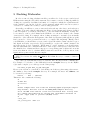
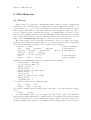
picked from the Colour Chart its name is printed to the terminal window. Shown below is
an example colour file 3hfl.col from the examples directory, which specifies the colours to
use when drawing an antibody/antigen complex. Subsets of the residues in each chain are
assigned different colours to highlight the positions of the antibody hypervariable loops:
L 1 214 grey
L 25 33 red
Chapter 3: Molecular Graphics
L 90
8
97 blue
H
H
H
H
1 225 RoyalBlue1
25 33 red
52 56 yellow
95 102 green
Y
Y
Y
Y
1 999 OrangeRed
41 53 yellow
67 70 red
84 84 blue
Colour files may also be used to colour atoms explicitly, using the syntax:
atom_name
first_atom
last_atom
colour_name
More sophisticated colour selection schemes could be implemented, but visualisation issues
get a rather low priority in Hex.
The Molecule Control panel also contains toggles to display molecular centroids and
average molecular ellipsoids. The ellipsoids are calculated from low order (L=2) spherical
harmonic surfaces. This control panel also allows the display of any crystallographically
related molecules whose coordinates are not given explicitly in the PDB file. Use the Symmetry Type selector to select these additional symmetry elements. Selecting Crystal causes
the scene to be generated using the SMTRY transformations from the PDB file, Biological
selects the transformations from the BIOMT records, and None (the default) just uses the
explicit atoms coordinates as usual. Note that atom coordinates are only replicated at display time using OpenGL display lists, so that even quite large molecules can be displayed
reasonably quickly. A fun one to try is the tobacco mosaic virus (PDB code 1RMV), especially when low resolution harmonic surfaces are enabled. Another nice structure is the
viral coat protein of the phi-X174 bacteriophage (PDB code 1CD3), which just happens
to be the 10,000th entry in the PDB. By selecting the File ... Save ... Symmetry ...
Biological option, Hex will write out all the symmetry-related atom coordinates when
saving a structure to disc. This is useful in cases where the biologically active molecule is a
dimer (or has some sort of symmetry) but only the minimal coordinate set appears in the
PDB data file. Some further editing of the output file (e.g. to rename duplicated chains)
may be required if the chains are to be individually coloured, for example.
3.2 Solid Models
The Graphics ... Solid Models control panel contains several options for drawing lit
solid models of molecular scenes, including van der Waals spheres, licorice, and tube representations. Aromatic rings may be drawn as hexagonal or pentagonal “blocks”, which can
produce some interesting displays, especially when viewing DNA molecules. The position
and colour of the light may be controlled using the controls in the Graphics ... Lighting
control panel.
Chapter 3: Molecular Graphics
9
3.3 Cartoons
The Graphics ... Cartoons control panel contains several options for drawing proteins
as ribbon cartoons. The default behaviour is to draw a cartoon over the molecular skeleton.
To view only the cartoon, you should can disable the molecular skeleton using the Display
Molecule button in the Controls ... Molecule panel.
The type of secondary structure within each protein chain is currently calculated using Frishman and Argos’ Stride (ftp://ftp.ebi.ac.uk/pub/software/unix/stride) program.
3.4 Solid Surfaces
Solid molecular surfaces may be drawn using the Graphics ... Solid Surfaces control
panel. These surfaces are calculated using a novel marching tetragons algorithm to contour
a Gaussian density representation of the atoms of each molecule. The surface skins used in
the docking correlations are calculated using this Gaussian density approach.
The Colour Mode selector allows surfaces to be coloured by atom colour (the default),
electrostatic potential or charge density, or by using the “classic” blue-red colour scheme
used in earlier versions of Hex. For electrostatic surfaces, a colour ramp is calculated which
initialy shows positive potentials/charges in blue, negative values in red, and intermediate
values in white. The Surfaces ... Colour Ramp button may be used to activate a simple
graphical controller for the colour ramp. The electrostatic potential and charge density
displays are calculated from the in vacuo global charge density expansion using the current
speherical polar docking expansion order, N.
The colours in a charge density display may appear somewhat “washed-out” compared
to (perhaps more familiar) potential displays. This is because the potential is calculated
directly from the charge density using Poisson’s equation, and the del-squared form of this
equation strongly emphasises any local variation in the charge density. So if the potentials
“look right” then the charge density is also correct. NB. Hex uses a relative permittivity
value of 8, instead of the more usual value of around 80. So, in addition to Hex ’s in vacuo
assumption, the numerical values for the potential are likely to differ from other software.
Some molecules may have internal cavities, and these can produce one or more contour surfaces in additional to the primary external surface. Other molecular structures
(e.g. structures with many waters, or well-separated domains) may also give multiple surfaces when contoured. As the contouring algorithm implicitly produces positively oriented
surfaces (outward normals, positive total volumes), it is convenient to assign each calculated surface to one of two possible classes: Primary (positive volumes, outward normals),
or Secondary (negative volumes, inward normals). By default, only Primary surfaces are
displayed, but this may be changed using the Draw Surface control.
In addition to the default Gaussian surface, the Surface Type selector provides the option to draw contoured density functions of the Sigma and Tau surface functions as used
by the docking algorithm. These two density functions allow the shape functions used in
docking calculations to be visualised. Sigma is the external skin density function, typically
calculated with a probe radius of 1.4 Å, and Tau is the interior density function (effectively,
the van der Waals volume). For relatively small molecules, and when using high expansion
Chapter 3: Molecular Graphics
10
orders (N), the Tau density can be seen to give a remarkably good representation of the
initial (atomic) Gaussian density. The order of the 3D expansion (default N=25) is taken
from the Docking ... Final Search parameter in the Docking Control panel. Both the
Sigma and Tau surfaces are contoured using a hard-wired density value of 0.25. However,
reconstructing each 3D density from the shape expansion coefficient vectors is a relatively
expensive calculation. This display mode is mainly intended to illustrate the internal representations used in docking.
The Sigma/Tau Shift slider controls how the shape (and electrostatic) expansion coefficients are computationally translated using the T(R) translation matrices prior to reconstructing the surface from translated expansion coefficients. Thus it is possible to view
graphically how the representation used in the docking correlation degrades with increasing
distance from the origin. In this display mode, the receptor surface is translated in the negative z direction, and the ligand surface is translated in positive z for ease of viewing. You
should see a blurring of those portions of each molecule furthest from the origin, although
the shapes of the surface regions near the origin are very well preserved after translation.
NB. In Hex ’s docking correlations, all computational translations are applied entirely to
the receptor.
Be aware that drawing surfaces can use a lot of memory. Drawing the surface of a large
molecule using a fine (0.25-0.5 Ångstrom) grid can use hundreds of megabytes of memory.
Attempting to draw a complex surface on a machine with insufficient memory could cause
the machine to hang.
3.5 Spherical Harmonic Surfaces
The Harmonic Surface control panel controls the way in which spherical harmonic molecular surfaces are calculated and displayed. Spherical harmonic molecular surfaces are generated from the dot surfaces calculated by Hex ’s internal dot surface algorithm, according to
the parameters set in the Harmonic Surface control panel. These parameters are distinct
from similar parameters in the Dot Surfaces control panel which generates dot surfaces
purely for visualisation (see Section 3.6 [Dot Surfaces], page 11).
When Hex calculates a spherical harmonic molecular surface, it first finds the shape
of an angular envelope which just enclosed all dots of the dot surface. This envelope is
made up of a list of approximately evenly spaced angular sample points (derived from
the vertices of a tessellated icosahedron), along with a radial distance from the origin to
the surface at the corresponding angular sample. Note that the surface envelope does not
properly handle multi-valued, or re-entrant, surfaces. That is, if a ray from the origin cuts
the molecular surface more than once, only the most extreme cut point is recorded for the
given angular sample. Nonetheless, this type of global envelope often gives a remarkably
good low resolution representation of most protein surfaces.
By default, the molecular envelope just described is not normally displayed. Instead,
Hex uses the sample points of the envelope to calculate a parametric representation of the
envelope using a spherical harmonic power series expansion. You can view the molecular
envelope by selecting:
Graphics ... Harmonic Surface ... Enable Surface (toggle on)
Chapter 3: Molecular Graphics
11
The sampling resolution is controlled by the Dot Density selector and the Mesh Order slider.
The dot density is the number of dots originally assigned to each atom in the dot surface
calculation. The mesh order controls the number of vertices in the icosahedral angular
mesh by defining the number of subdivisions along each edge in the original icosahedron.
The Probe Radius slider may be used to modify the size of the probe sphere used in the
initial dot surface calculation. Setting a probe radius of zero would give a van der Waals
surface, instead of the molecular surface. The envelope may be displayed in different styles
and colours using the Display Mode and Line Colours selectors. By disabling the envelope
display and by enabling spherical harmonics, one can view the corresponding spherical
harmonic molecular surface:
Graphics ... Harmonic Surface ... Enable Surface
Controls ... Harmonics ... Enable Harmonics
(toggle off)
(toggle on)
In fact, these are Hex ’s default settings, so that once a molecule has been loaded, pressing
the Harmonics button on the right hand border calculates and displays a spherical harmonic
surface directly. The order of the spherical harmonic expansion can be selected using the
Order (L) slider in the Harmonics Control panel.
3.6 Dot Surfaces
These days, dot surfaces are somewhat of a historical remnant in Hex. They used to be
used as an approximate but fast way to calculate the molecular surface, the solvent-accessible
surface and the van der Waals surface for docking. However, docking and superposition
calculations now use a much more accurate method based on contouring Gaussian density
functions to calculate these two surfaces. Nonetheless, its still sometimes useful to be able
to draw dot surfaces. If nothing else, dot surfaces give a fast way to verify that Hex is
recognising all the atoms in a PDB file because sometimes unrecognised atoms may not
be drawn in the other drawing modes, whereas the dot surface calculation always uses all
atoms, regardless of their type. Spherical harmonic surface envelopes are also calculated
from the sampled dot surface.
The calculation and display of dot surfaces is controlled by settings in the Dot Surface
control panel. The short-cut Dots button on the right-hand border of the main window
provides a fast way to toggle the display of dot surfaces. By default, Hex displays a molecular
surface calculated using a 1.4 Ångstrom radius probe sphere.
Dot surfaces are calculated by covering the surface of each atom with a set of sample
points generated from an icosahedral tessellation of the sphere. The default dot density is
162 dots/atom, but this may be changed using the Dot Density selector. Any dots which
are occluded by neighbouring atoms are immediately discarded. If the Probe Radius is
zero, then this gives the van der Waals surface. Otherwise, the program calculates the
molecular surface and solvent-accessible surface by rolling a probe sphere over the surface
(non-occluded) atoms of the molecule.
When Hex calculates a molecular surface, non-occluded atom dots are classified as one of
convex-accessible, toroidal-reentrant or singular-reentrant. These classifications correspond
to the type of contact the dot should make with a probe sphere being rolled over the
molecule. The convex-accessible dots are those which may be touched by the probe when
the probe sphere is not simultaneously in contact with any other atom. All other dots
Chapter 3: Molecular Graphics
12
are considered as reentrant. Reentrant dots are then “pushed out” from the atom surface
to meet the locus of the molecular surface. The position of the reentrant surface can be
calculated by a 2D analysis of the path of the probe sphere for toroidal dots and by a
similar calculation using the 3D stationary probe positions for the singular points (when
the probe simultaneously touches 3 or more atoms). Without going into more detail here,
the algorithm is exact when an infinitely small probe is used but the quality of the resulting
surface degrades as the probe size increases. This is because there is only a fixed number
of dots with which to populate the re-entrant surface regions. However, this degradation
is hardly noticeable with probe radii up to about 1.5 Ångstroms. Since the dot surfaces
produced here are primarily for computational rather than visualisation purposes, a modest
degree of inaccuracy is quite acceptable.
The type of dot surface which is actually displayed is controlled by the Skin Factor slider.
Setting the skin factor to zero causes the molecular surface to be displayed: a skin factor
of one draws the solvent-accessible surface. Intermediate values cause dots to be drawn at
the corresponding fraction along each of the outward surface normals. The Display Mode
may be changed from dots to vectors, in which case surface normals are drawn as lines of
the length implied by the current skin factor. Vectors are drawn as dots if the skin factor is
zero. Dots (or vectors) may be coloured according to atom type or a colour may be selected
from the colour chart using the Dot Colours selector.
3.7 Changing The Scene Origin
Normally, rotation and scale (zoom) operations are applied relative to the scene origin. When just one molecule is loaded, the scene origin coincides with the centroid of
the molecule. However, when two molecules are loaded, the scene origin is taken as the
midpoint between the two molecular centroids. This behaviour can be changed by using
the first selector in the Orientation Control panel to select a given molecular centroid or a
specific atom to act as the origin. The Select Origin button (a circle with a diagonal cross
through it) on the left hand border may also be used to select the zoom/rotation centre.
Although docking calculations normally move both the ligand and the receptor, the
default display behaviour is to keep the receptor fixed in space and to assign all the motion
to the ligand as successive docking solutions are viewed. This behaviour can be changed
using the Docking Motion selector in the Orientation Control panel.
3.8 Clipping The Scene
The Clipping button (three faces of a cube) on the left hand border selects scene clipping
mode. You can define up to six clipping planes in the scene, several of which may be moved
together using a single slider. However, controlling clipping is probably the most difficult
part of the program to master, since this involves the use of all three mouse buttons and
several keyboard keys, in addition to the basic graphical widgets.
When scene clipping mode is selected, you should see a wire frame drawing of six skeletal
clipping planes centred in the scene. A new slider control is also drawn in the bottom right
border. This new slider may be used to move selected clipping planes through the scene, in
plane-perpendicular directions.
Chapter 3: Molecular Graphics
13
In clipping mode, the mouse buttons may be used to translate and rotate the clipping
skeleton in the usual way. Note however, that the rest of the scene remains fixed. You can
use the keyboard Space Bar to toggle between moving the skeleton about the scene and
moving the scene about the skeleton.
Picking one of the skeletal planes (using Button 1 for picking) selects that plane and
attaches it to the scene. The plane is now drawn in white, either as a filled shape or as an
outline, depending on which face you happen to be viewing. The mouse buttons now move
only this plane relative to the scene (or, if you have hit the Space Bar, the mouse moves the
plane and the scene together). The filled face will become the clipping face of that plane.
Button 2 may be used to activate the selected plane (just press Button 2 anywhere in the
scene). That is, every part of the scene above the filled face should become clipped. Pressing
Button 2 again toggles clipping. Try moving the clipping plane though the scene using the
right slider, or by using the mouse and the Space Bar to control the movement. Try using
the Delete Key (keyboard backspace) to toggle the sense of the clipping plane. Once you
are happy with the position of the clipping plane, you can revert to Pointer Mode (select
the Left Arrow button) or you can proceed to pick and activate further clipping planes.
In pointer mode, the right hand slider continues to operate the most recently activated
clipping plane.
It is also possible to make the slider move two planes simultaneously. Having activated
a clipping plane, now try picking it with Button 3. This draws the plane in yellow and ties
its motion to the slider. Now pick and activate the clipping plane (using Buttons 1 and 2)
on the opposite face of the clipping skeleton. The right slider should now move both planes
together through the scene. You can tie multiple planes to the slider, although selecting two
perpendicular planes is probably the most sensible option. As you might expect, picking a
plane with Button 3 for a second time unties it from the slider.
At any time while in clipping mode, you can undo the most recent operation using the
Hammer button. Three successive clicks on the Hammer will clear all clipping settings and
will return the display to an unclipped scene.
If necessary, you can use the keyboard Plus and Minus keys to zoom the clipping skeleton
independently of the scene. If the scene contains molecular surfaces (dots, lines or polygons),
you can use the keyboard Equals key to toggle between clipping both the molecule and its
surface (the default) and clipping just the surface, leaving the molecular skeleton fully
visible.
3.9 Animation
The Animation Control panel allows you to run a “movie” of either the results of a
docking calculation, or a sequence of models from an NMR structure, for example, and it
controls how the scene “spins” if you perform a mouse drag-release action.
After a docking run, pressing Start in the Graphics ... Animation control panel will
cause Hex to draw each docking solution in turn. The rate at which orientations are
drawn is controlled by the Frame Rate slider. Similarly, if you have loaded a PDB file
that contains several NMR model structures, setting the Movie Type to Receptor Models
or Ligand Models, as appropriate, and pressing Start will show a movie of the sequence of
models. The orientations, or frames, of both types of movie may be shown just once, or
Chapter 3: Molecular Graphics
14
cycled forever. The movie can be stopped at the current frame by pressing the Stop button.
The speed of the movie is controlled by the Frame Rate slider.
The maximum frame rate achievable will depend on the speed of the CPU and on whether
your machine has hardware-accelerated graphics. The Frame Rate thus defines a requested
rate. Actual performance will vary. But please note, Hex never hogs the CPU in a tight
loop on input events, even during an animation, as do many other programs (which shall
remain nameless). Thus it should still be possible to perform other activities while a movie
is running without things becoming sluggish.
You can spin the scene by dragging with Button 1 or Button 2 to start a rotation
and by releasing the button while still moving the mouse to initiate a continuous rotation
(spinning). When spinning, the rotatation angle is incremented by the current value in the
Spin Angle slider, and new rotational increments are drawn at the current Frame Rate. If
desired, the mouse button action that initiates spinning can be enabled/disabled with the
Enable Spinning toggle. Spinning is enabled by default, and it is possible to spin a movie
(if thats what you really want to see!).
Any of the usual user interface controls may be used while an animation is running. If
using these controls changes the graphical complexity of the scene, Hex will take a second
or two to adjust the drawing speed back to the requested frame rate.
3.10 Full Screen Mode
Personally, I think full-screen mode is the best way to view molecular graphics scenes.
You can press F to switch back and forth between full-screen and window-manager modes.
By default, Hex starts in window-manager mode. You can also press G at any time to toggle
the display of the GUI controls when in full-screen mode. G only toggles the setting, not
the display. So you won’t see the effect until you enter full-screen mode.
In both the Unix and Windows versions, you should always use F to get full-screen mode
because this forces the window border off. Conversely, don’t use the window manager’s
“maximise” control because this forces the window to keep a border, and F won’t then
work.
In Windows XP, you will probably still see the Windows Taskbar in full-screen mode.
To get rid of this, open the Taskbar and Start Menu in the Windows XP Control Panel
and uncheck the Keep the taskbar on top of other windows item. I don’t know whether this
feature is available on earlier versions of Windows.
In Mac OS X, full-screen mode does not override the Mac Taskbar and Dock panels.
Hence it is best not to use Hex ’s full screen mode, but instead use the window manager’s
“maximise” button to ensure the graphics window is well-behaved.
On Linux (Fedora/RedHat), full-screen GUI mode with the Gnome window manager is
“quirky”. Everything works as it should, except that Hex control panels can’t be re-raised
over the full-screen window after the control panel loses mouse focus (i.e. when the cursor
leaves the panel). You will need to revert to window-manager mode (F) to see everything
again! I don’t know what other Linux window managers might do, but it seems many
window managers don’t handle full-screen windows very well!
Chapter 3: Molecular Graphics
15
3.11 Stereo Displays
Stereographic displays should work on systems that support “stereo-in-a-window”
(untested on SGI and Sun). Stereo is known to work on Windows XP and RedHat Linux
8.0 (kernel version 2.4.18-14, XFree86 version 4.0.0) or later with an nVidia Quadro4
XGL700 card, and using a recent nVidia driver (1.0.3123 or later).
For best results with Hex and nVidia cards, please use the latest versions of both driver
software, service packs, and operating systems. The recent nVidia drivers give Hex both
stereo-in-a-window and full-screen stereo on both Windows XP and Linux. nVidia’s 4351
driver (May 2003) is excellent, and is very easy to install. See Appendix D [nVidia Stereo
Configuration], page 49 for more details. However, if you are upgrading an nVidia driver
on Windows, ensure you de-install any earlier drivers first. I caused myself significant grief
by not doing this!
The type of graphics visual that Hex uses is determined when the program first starts
up. By default, Hex tries to use a stereographics window. However, this nearly halves the
drawing rate compared to non-stereo drawing. So if you don’t like/want stereo, you can
force stereo off by using hex -nostereo. Alternatively, set the HEX STEREO environment
variable to a false value (i.e. any one of: no, n, false, f, or 0) in your login script. If
a stereo visual has been selected, the display may be toggled between stereo and mono
using the Stereo Parallax option in the Projection Control panel (or simply by pressing the
keyboard S key). The Parallax slider may be used to adjust the stereographic effect. Stereo
parallax is the perceived separation between the left and right images in the viewing plane
(monitor screen). The numerical values in the parallax slider correspond approximately to
screen millimetres on an un-zoomed display. Positive parallax values make the scene appear
“inside” the display, whereas negative values cause the scene to appear through, or in front
of, the plane of the display. A better stereographic effect is achieved when the Perspective
Projection toggle is enabled (by default, an orthographic projection is used). The keyboard
P key may also be used to toggle between perspective and orthographic projection modes.
When perspective is enabled, a checker-board background may also be enabled to enhance
the perspective effect (keyboard B). The perspective effect can be increased by reducing the
Far Plane and/or increasing the Near Plane slider values. For most people, a small positive
parallax and a moderate perspective gives a pleasing effect without straining the eyes.
For PC/Linux stereo, you should download the shared-link executable (see Section 6.10
[Technical Information], page 37) because hardware stereo support is currently only available
in the vendor-supplied GL/GLX libraries. Even if you don’t have hardware stereo, you may
still get better graphics performance using the shared-link executable if your graphics card
has hardware-accelerated OpenGL support.
Chapter 4: Manoeuvring Molecules
16
4 Manoeuvring Molecules
In addition to rotating, translating, and scaling a molecular graphics scene, Hex, also
allows you to change the relative orientations of a pair of molecules. Hex calls this editing,
because saving “manoeuvred” structures out to a file causes them to be written using their
transformed coordinates. Note: Edit Mode is only enabled when you have two molecules
loaded. Editing is often a necessary preparatory step before running a docking calculation.
For example, when you load a pair of molecules, Hex uses some heuristics to place the
ligand near the receptor. However, you may have knowledge about one or both of the
binding sites, and hence you may want to manoeuvre the molecules into something that
resembles the expected binding orientation. If you do this, you can then limit the search
range of the docking correlation instead of performing a global search. This should give
fewer “false-positives”, and it will certainly make the docking calculation go faster.
TIP: In the graphics, you can edit both the receptor and the ligand orientations, but
the coordinates of the receptor “take priority” when structures are saved to disc. In other
words, any relative motion is always transferred entirely onto the ligand on output. The
receptor coordinates are always restored to their original values.
4.1 Editing Orientations
There are two main ways to edit molecular orientations within the scene. In the first
method, using the Orientation Control panel, a molecule may selected using the Apply to
selector and then rotated using the Euler angle Alpha, Beta and Gamma sliders. The intermolecular separation can be modified with the R slider at the bottom of the main window.
Select Commit when you’re done editing, in order to commit the new transformations into
the molecules. In the second method, editing can be performed by manually manipulating
the scene with the mouse by pressing the Edit Mode button (which looks like a lightning
bolt) in the left border. This method can also be used in conjunction with the Orientation
Control panel.
In both editing modes, picking a molecule ties its motion to the mouse and to the rotation
sliders in the Orientation Control panel. The bonds of the picked molecule are displayed as
dashed lines as a visual reminder that this molecule has been activated for editing. Picking
the background (i.e. a Button 1 pick that misses all atoms) de-selects the active molecule
and makes the mouse move the whole scene. The Hammer button can be used to undo
the most recent sequence of editing movements. When editing molecular orientations, it
may help to activate the Intermolecular Axis. Once you’re happy with your edits, revert to
Pointer Mode to commit the new orientations. You can now save the scene by going to the
File menu and selecting:
File ...
Save ... Both
This causes a file selection widget to appear, prompting you for the name of a file in which to
save both molecules (in the newly edited orientation). You can confirm the new orientation
has been created by loading the new file into another Hex session (you may have to rotate
the scene to see exactly the same view). Alternatively, you could write each molecule to a
separate file using:
Chapter 4: Manoeuvring Molecules
File ...
17
Save ... Receptor
and
File ... Save ... Ligand
You could then open these new files to verify the new orientation.
You may want to try using these editing features to manually dock the ligand into the
receptor binding site (if appropriate), or you might try to superpose the two molecules, if
they are similar. Neither task is easy!!
4.2 Editing Centroids
When Hex reads in a molecule, it uses its all-atom centre of mass as its centroid. This
centroid is used as the local coordinate origin for docking, and as the point about which any
molecular rotations are applied. However, if one or both molecules are quite large (i.e. too
big to fit within about a 30 Ångstrom radius ball), you will probably want to change the
centroids used for docking. This is because Hex ’s radial functions fall off rapidly beyond
about 30Å from the origin. Hence, unless you move the origin(s) to be closer to the expected
binding site(s), you are likely to get very poor docking results. If you don’t know or suspect
where the binding site is on a large molecule, you should use Hex ’s macro docking mode
for such cases. See Section 5.11 [Macro Docking], page 25.
Molecular centroids may be edited using the Edit Origins button (two crosses and a
line) on the left-hand border. Try changing to Edit Origins mode, and pick a molecule
to edit. Once the picked molecule is highlighted, dragging Button 1 will move the origin
of the selected molecule. As with editing orientations (above), it may help to activate the
Intermolecular Axis in order to see the new and old positions of the centroid(s). In Edit
Origins mode, buttons 2 and 3 always rotate the entire scene. When you revert to the
default Pointer Mode, the new origin will be activated. Note that the new origin only
applies to the current session. It is not saved when you write an edited molecule to disc.
TIP: You can use virtually all of the other GUI functions while in edit mode, although
certain operations (e.g. opening/closing molecules) cause Hex to revert to pointer mode.
Chapter 5: Docking Molecules
18
5 Docking Molecules
In order to run a docking calculation in Hex, you will need to load a receptor and a ligand
PDB structure using the File pull-down menu. If you want to test the docking algorithm by
docking two separately determined sub-units of a complex for which the crystal structure
is also available, you can also load the complex structure which will be used as a reference
orientation to evaluate the accuracy of the docking prediction.
Generally, you will have to remove water molecules and any other hetero molecules prior
to docking. You can do this globally using the Hetero Control menu panel. If more detailed
control is required, you will probably have to edit each PDB file manually. It may also
be necessary to remove other chains in the PDB file or to shorten a chain to the domain
of interest in docking. For example, when docking an antigen to an antibody it is usually
advisable to delete all but the Fv fragment of the antibody structure (although the program
has been used to dock a protein G molecule to a complete Fab fragment). Having edited
your PDB files, you should have a receptor and a ligand file which contain only the receptor
and ligand molecules, respectively, and (optionally) a complex file, which contains both
molecules in the docked orientation. When using a complex structure, you should ensure
that the chain names are consistent with those of the receptor and ligand because Hex uses
the chain labels to identify and hence superpose corresponding pairs of alpha-carbon atoms
from each chain in order to calculate RMS deviations between the docked position of the
ligand and its position in the known complex.
TIP: You can use the utility hex chain in Hex ’s bin directory to rename a chain in a
PDB file.
Up to three protein structures can be loaded into Hex directly from the command line.
For example, to load three of the PDB files from the examples directory for the HyHel5/lysozyme complex, you could type at the Unix prompt:
hex 3hfl_fv.pdb 3hfl_ly.pdb 3hfl.pdb
However, its often more convenient to load all three molecules together using a short macro
file, similar to those in the examples directory. For example, the macro file, 3hfl.mac, can
be executed by selecting:
Macros ... Run ... 3hfl.mac
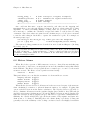
This macro file contains the following:
#
# 3hfl.mac
# ========
#
# This example macro file loads the antibody HyHel-5/lysozyme complex.
# By default, Hex will look in the $HEX_ROOT/examples directory
# for the PDB files and the colour file referenced here. You may wish
# to change this behaviour by setting some environment variables in
# your .login (csh) or .profile (sh/ksh) files.
#
close_all
set_colour_file 3hfl.col
Chapter 5: Docking Molecules
19
open_receptor
3hfl_fv.pdb
open_ligand
3hfl_ly.pdb
open_complex
3hfl.pdb
fit_ligand
When using a complex reference structure, you should find that on loading the molecules,
the complex is drawn in grey and the receptor molecule is superposed onto the appropriate
part of the complex. If the ligand molecule originated from an edited complex file, then
it will be superposed over the complex (because its coordinates are relative to the same
coordinate frame as the receptor molecule). Otherwise, the ligand can be transformed into
the receptor/complex frame using the Fit Ligand button in the Orientation Control panel.
5.1 Rotational Search
Hex currently supports three docking search modes, which may be selected using the
Search Mode selection box in the Docking Control panel. Most docking problems require
only the default Full Rotation mode, in which the receptor and ligand are effectively rotated
about their own centroids, and the ligand is twisted about the intermolecular axis at each
of a range of intermolecular distances. Thus the default behaviour is to perform a full sixdimensional search over the full rotational ranges. However, more limited docking searches
can be performed in which the allowed angular and distance ranges may be constrained by
the user. The calculation is arranged so that the intermolecular twist angle search is in the
innermost loop of the algorithm. This innermost loop turns out to involve a sum over sines
and cosines of the twist angle, which may be accelerated using a one-dimensional FFT.
There are several controls which specify the resolution, and in particular the order, N,
of the docking correlation. The default settings are for the program to perform an initial
Steric Scan at N=16, followed by a Final Search at N=25, using just the steric contribution
to the docking energy. In this mode, about all but the top 20,000 orientations are discarded
after the Steric Scan. The Steric Scan may be toggled off, in which case every orientation
is evaluated using a steric correlation (and optionally an electrostatic correlation) to order
N, as given the Final Search slider. However, this can significantly increase total docking
times. Using the two-step search with N=16 and N=25 is found to work well in practically
all cases. The electrostatic contribution to the docking correlation may be enabled using
the Electrostatics toggle. Electrostatics are only ever calculated in the Final Search phase.
You can get a feeling for how well each correlation order, N, recognises a given complex by
running the program on known complexes and by observing how highly the correct solution
is ranked in each case.
NB. Although the default is to use correlations to N=25, in Rounds 3–5 of the CAPRI
blind trial (http://capri.ebi.ac.uk/), I found that better results are obtained using
N=30 correlations (see Section 6.14 [References], page 39).
5.2 Other Search Modes
In addition to the basic rotational search, Hex also supports a Ligand Translation and
a Ligand Orbit search mode. In Ligand Translation mode, the receptor is held fixed and
the ligand is translated about the receptor using the Ligand Range and Samples angular
Chapter 5: Docking Molecules
20
parameters and the Distance Range and Step parameters to generate different ligand poses
about the receptor. A pure translation is achieved if the twist angle is set to zero.
In Ligand Orbit mode, the ligand is translated as above, but it is now also rotated about
its own principle axis (in fixed steps of 10 degrees). A “wobble” may be added to the
search by setting a small range (say 30 degrees) for the twist angle. These search modes are
largely experimental, but may be useful if the relative orientation of a pair of molecules in
a complex is known but the exact binding mode is not.
These modes are less efficient than the default rotational search mode since they can’t
exploit the fast (FFT) twist angle search on the innermost loop of a rotational docking
search. If in doubt, use the default Full Rotational search mode.
5.3 Distance Sub-Stepping
As of version 4.5, Hex performs the high resolution Final Search correlation using smaller
distance incerements than are used for the fast low resolution Steric Scan phase. This
allows the search space to be covered more rapidly (coarsely) in the first phase, but more
finely in the final phase. This behaviour is controlled by the Distance Range, Scan Step
and SubSteps parameters in the Docking Control panel. The default values are Distance
Range=40, Scan Step=1.0, SubSteps=2. This means that the Steric Scan phase will search
over 41 distance increments (20 steps of +/- 1 Å from the starting separation, plus the
starting separation itself). These orientations are sorted by calculated energy, and a new
set of trial orientations are generated for the top-scoring 10,000–20,000 orientations using
the Scan Step and SubSteps parameters to construct new distance samples in steps of +/(Scan Step)/(Substeps) from the initial orientations. In other words the default behaviour
is essentially to scan the search space at 1 Å resolution, but to perform the high resolution
scoring at 0.5Å resolution. Setting SubSteps=0 gives the old behaviour of earlier versions
in which a constant distance step is used for both resolution levels.
5.4 Radial Filters
When performing a full 6D docking search, the most expensive part of the calculation
is normally the initial steric scan. This phase can be accelerated by selecting a Radial
Envelope Filter in order to avoid scanning orientations in which the molecules overlap significantly, or are too far apart for ther surfaces to interact. There are two radial filtering
modes, which both use low resolution spherical harmonic surface envelopes to define an
approximate radial envelope for each molecule. The surfaces are constructed using the current expansion order (default L=12) from the Controls ... Harmonics ... Order selector.
The Re-entrant filter assumes each molecule is fully contained within the harmonic surface,
and excludes trial distances at which the surfaces are too far apart. The more aggressive
Star-like filter assumes the surfaces are single-valued with respect to a ray from the origin,
and additionally excludes trial distances at which the surfaces are presumed to be too close
together for docking to be feasible. It is unwise to use these filters if either docking partner
is non-globular.
Chapter 5: Docking Molecules
21
5.5 Docking Examples
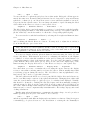
OK, lets start docking. Open the Docking Control panel and select the following (mostly
default) values from the selection boxes:
Controls
Controls
Controls
Controls
Controls
Controls
Controls
Controls
Controls
Controls
Controls
Controls
Controls
...
...
...
...
...
...
...
...
...
...
...
...
...
Docking
Docking
Docking
Docking
Docking
Docking
Docking
Docking
Docking
Docking
Docking
Docking
Docking
...
...
...
...
...
...
...
...
...
...
...
...
...
Grid Dimension ...
Solutions ...
Receptor Range ...
Ligand Range ...
Receptor Samples ...
Ligand Samples ...
Twist Range ...
Twist Samples ...
Distance Range ...
Distance Step ...
Substeps ...
Steric Scan ...
Final Search ...
0.6
500
30
30
642
642
360
128
40
1.0
2
16
25
This says that the Steric Scan (N=16) phase of the docking calculation will be performed
at 1+40/1.0=41 intermolecular separations, in +/- steps starting from the current distance
posted in the R slider in the bottom border of the main window. The Final Search (N=25)
phase will be applied to the the highest scoring scan orientations in steps of 1/2 Å, as
described above. The angular search will be restricted to 30 degree angular cones centred
on the intermolecular axis, and the best 500 solutions will be retained for viewing.
Now start the calculation:
Controls ... Docking ... Activate
You’ve just started an example docking search restricted to the known binding sites, so the
calculation should only take a few minutes. The program will take a few seconds to calculate
the surface skin coefficients and then proceed to calculate docking correlation scores at each
of the specified angular and intermolecular increments. A Cartesian grid is used to sample
the molecular skins numerically but this grid plays no further role in the calculation once the
surface skin expansion coefficients have been determined. Most conventional FFT docking
algorithms have to use rather large grids (e.g. 1 Ångstrom cubes) because the grid must
accommodate all possible translations of the ligand about a stationary receptor. Here, the
grid only needs to contain the larger of the two molecules so that much finer sampling grids
are feasible. In Hex, a 0.6 Ångstrom grid seems to work well and is still reasonably fast to
calculate. The sampling grid size may be varied using the Grid Dimension selection box.
The calculation of the surface skins used in the docking correlation is controlled by the
parameters in the Surface Control panel. The default values do not normally need to be
changed.
The search in the above example is “restricted” because setting the ligand and receptor
range angles to 30 degrees means that only a small fraction of the 642 rotational increments
(the Receptor Samples and Ligand Samples values) will actually be used for the molecular
rotations of each molecule. These rotational samples are generated from an icosahedral
tessellation of the sphere and, in this case, have an angular separation of about 8.5 degrees
between each sample point. Essentially, each molecule is rotated incrementally so that
Chapter 5: Docking Molecules
22
successive tessellation points are rotated onto the intermolecular axis (the z-axis). Thus, in
the low resolution Steric Scan phase, 642 x 642 distinct rotational orientations are produced,
although any orientations that fall outside the angular range cones are discarded. At each
of the surviving orientations, the ligand is then rotated (or twisted) through 360 degrees
about the z-axis in 64 steps of about 5.6 degree increments specified by the Twist Samples
value. In this constrained example, Hex will evaluate the docking score at each of 46 x
46 x 64 = 135,424 distinct rotational orientations, with the calculation being repeated at
each of the 41 intermolecular distances implied by the distance range and step parameters.
In the high resolution Final Search phase, the best 10,000 of the above orientations will
be used to generate 25,529 new distinct trial orientations after distance sub-sampling (see
above) and re-evaluated at N=25 using 128 samples for each twist angle search. Note, Hex
is hard-wired to use 64 twist steps in the initial steric scan phase, because there no benefit
in using finer steps in this phase.
It should be noted that such docking calculations never give a unique solution. Rather,
Hex sorts the generated orientations by docking energy and prints a summary of the 10,000
highest scoring (lowest energy) orientations. The best 500 orientations are retained for
viewing. You can view the solutions using the Soln: slider, or you can step through the
solutions using the keypad or arrow keys:
Home:
Page/Down:
Page/Up:
End:
Starting orientation
Next solution
Previous solution
500’th (or last) solution
You should find in the above example that Hex generates several orientations with low
RMS deviations from the correct (starting) orientation. However, you might object that
the calculation was biased to find the right answer by restricting the search to the known
binding sites. If so, you could try a global docking search (about trial 10^9 orientations),
using:
Controls ... Docking ... Receptor Range ...
Controls ... Docking ... Ligand Range ...
180
180
This calculation will take about 30 minutes on a single 1GHz Pentium III processor. This
is substantially faster than an equivalent calculation using a conventional FFT approach.
In this particular case, Hex should still identify the correct docking orientation (to within
about 1.5 Ångstrom RMS), but its often useful to use restricted searches when starting with
unbound subunits.
TIP: When viewing docking solutions, its helpful to keep either the receptor or the
ligand in a fixed orientation in the display, so that only one molecule moves when stepping
through the docking solutions. The default is to transfer any receptor motion onto the
ligand, so that the ligand appears to translate and rotate about a fixed receptor. This
behaviour can be changed using the Orientation Control panel:
Controls ... Orientation ... Centre ... Ligand
Chapter 5: Docking Molecules
23
TIP: If you plan to use Hex more than once, enabling a disc cache will speed up the
translational part of each calculation. When disc caching is enabled the (large) translation
matrices are calculated only when necessary and are saved in the cache directory for re-use.
Disc caching controls can be found under the File menu. The default cache directory is
$HEX ROOT/cache, although it is recommended to set a cache directory explicitly using
the HEX CACHE environment variable. The cache directory should be specially created
for this purpose (i.e. it contains nothing else) and a distinct directory should be used by
each user (because there’s no synchronisation between multiple invocations of Hex ). With
typical usage, the disc cache will occupy from 50 to 200 Mb of disc space.
5.6 Calculating Bumps
Following the basic docking correlation algorithm, candidate docking orientations may
be filtered and refined using one of the Post Processing options. Post processing is applied
to the top-scoring 1,000 solutions from the correlation search (or the user-selected number
of orientations to retain, if larger than 1,000). The simplest option is to enable a bumps
counter, in which the number of steric clashes between non-bonded pairs of heavy atoms in
each solution is calculated. An option in the Clustering Control panel may then be used to
filter out solutions with a specified number of steric clashes.
5.7 Molecular Mechanics Refinement
In addition to the bumps counter, a single (rigid body) molecular mechanics energy
may be calculated for each docking solution (MM Energies), or a Newton-like energy miminisation (MM Minimisation) can be applied to each docking solution. These energies
are calculated using “soft” Lennard-Jones and hydrogen bond potentials, adapted from the
OPLS force-field parameters, along with an explicit charge-charge electrostatic contribution. When docking complexes where conformational changes are known to be small, this
gives an effective way to prune many “false-positive” orientations and to enhance the energy
of the “right answer”. However, this rigid-body refinement procedure should not be used if
conformational changes are expected to be large because (despite using soft potentials) it
tends to eject ligands with incorrect conformations from the binding site. This part of the
program is still “under development”.
5.8 Clustering Docking Results
Because Hex uses essentially a brute-force search approach to the docking problem, it
is advisable to over-sample the search space rather than to risk missing a good solution by
under-sampling the space. However, this can cause multiple similar but incorrect orientations (false-positives) to push good solutions down the list. By default, Hex uses a simple
clustering algorithm to group spatially similar docking orientations. Each docking solution
is first ordered by energy, and the lowest energy solution is made the seed orientation for the
first cluster. The list is then searched down to a given depth for other similar orientations
whose main-chain alpha-Carbon RMS deviation is within a given threshold (default 2 Å
RMS) of the seed orientation, and these orientations are then assigned to the first cluster.
The process is then repeated starting from the next lowest unassigned orientation, until all
solutions have been assigned to a cluster. The Cluster Window parameter may be used to
Chapter 5: Docking Molecules
24
control the search depth when looking for cluster members. Because clustering uses a simple
but inefficient algorithm (rather like a “bubble-sort”), it is advisable use this parameter to
limit the search depth if the number of saved solutions is large.
The Controls ... Clustering control panel may be used to control the type of clustering and clustering parameters used, and how cluster membership affects the displayed
solutions. By default, only the lowest energy member of each cluster is displayed or written
to an output PDB file (Display Clusters = Best). Alternatively, you can choose to view (or
output) all solutions (Display Clusters = All). Similarly, solutions may be viewed in cluster
order (best to worst) or in order of calculated energy using the Sort Solutions selection option. The RMS threshold for cluster membership may be changed using the RMS Threshold
slider. Displayed solutions may also be selected by the number of steric clashes, or bumps,
detected. Any solution containing a number of bumps which is less than or equal to the
current Bumps Threshold (default 0) is a candidate for cluster membership. Solutions with
a greater number of bumps may still be viewed or output, but these always appear after
any non-bumping solutions in the sorted list of solutions (i.e. have a larger cluster rank).
The default docking search range and clustering parameters are normally sufficient to
generate good coverage of the search space, and to distinguish different but similar solutions. But you may wish to experiment. Clustering is re-calculated whenever a clustering
parameter is changed, without having to re-run the docking search. Here, “good coverage”
means that for each docking orientation, there is about a 99% chance of generating at least
one other solution within 3Å RMS of the first one (unpublished experiments). Deciding
whether or not two similar but different orientations ought to fall within the same cluster
is somewhat subjective. The 2Å threshold seems to work well for large-ish ligands (roughly
100 residues), but should probably be reduced for smaller ligands.
5.9 Saving Docking Results
There are two main ways in which docking results may be saved to disc. The most
compact method is to write a docking summary file using the File ... Save ... Transform
menu item. This writes a file that lists the docking energies for all predicted orientations,
along with the rotation and translation parameters wich should be applied to the ligand
coordinates in the original ligand PDB file in order to produce the corresponding docking
orientation in the coordinate frame of the recptor PDB file. The actual file format is
descibed in the first few “comment” lines of the output file. A similar but more detailed
output file format is given by File ... Save ... Matrix. This lists the transformations in
a more verbose format using keywords to label each piece of data. For rigid body docking,
bot formats are quite compact, but you will need to write your own code to process the
docking summary file. Its not possible to read these files back into Hex ; they are purely for
output to external software.
The second, less compact output method is to write a separate PDB file for each docking
orientation. The current docking orientation can be written to a single PDB file by selecting:
File ...
Save ... Both
Alternatively, a range of docking solutions may be saved using:
File ...
Save ... Range
Chapter 5: Docking Molecules
25
This opens a new Save Docking Range panel in which a range of docking solutions may be
specified, along with a a file name pattern to be used for the output files. The default is
to save the first 100 solutions to separate PDB files of the form dock001.pdb, etc., in the
current directory.
In both the PDB range and the summary output modes, either a list of raw solutions
(sorted by energy) are written, or a range of clustered orientations are written, depending
on the current clustering option. In other words, the sequence of solutions written out is
the same sequence that you would see when stepping through the orientations using the
Page/Down and Page/Up or arrow keys.
5.10 Docking Multiple Structures
Docking multiple structures (e.g. NMR structures) with Hex is easy. Just put all your
ligand structures (assumed to be in a common coordinate frame) into a single PDB file, and
use the PDB convention of MODEL/ENDMDL to distinguish each structure. Hex will run
its docking search for each ligand in turn. Similarly, multiple receptor model structures may
be loaded and docked, giving an M by N docking (may take a while though!). The actual
structures to be docked may be selected using the Receptor Docking and Ligand Docking
selectors in the Controls ... Solid Models control panel (default all v’s all). Individual
structures may be selected for viewing using the Receptor Display and Ligand Display
selectors in the same control panel. This panel also contains some experimental controls
for cloning and editing different models (where each clone is treated as a new NMR-type
model structure to be docked, with each docking run each starting from the edited pose).
5.11 Docking Very Large Molecules (Macro Docking)
The radial shape functions used in Hex decay exponentially beyond about 35 Ångstroms
from the chosen origin. This means that the shapes of proteins much larger than this are
not represented well. One example of such a large protein is the viral-surface hemagglutinin
molecule presented in the CASP II and CAPRI protein docking challenges. In order to dock
such large molecules, Hex assigns multiple local coordinate systems to the larger molecule
(assumed to be the receptor ) and docks the ligand around each local coordinate frame on
the receptor. Setting up the receptor coordinate systems is controlled by the Controls ...
Macro-Sampling control panel.
The general approach is to construct a very low resolution spherical harmonic surface
representation of the receptor (say, setting L=5 in the Harmonics Control panel), and then
to cover this surface with a large number of spheres. These spheres are placed using the
surface normals of each triangular patch used to draw the harmonic surface. The spheres
are then iteratively culled, where the sphere with the greatest overlap with its neighbours is
culled at each iteration. This is repeated until some pre-set number of spheres (default 25)
remain - these should still cover the surface, but be reasonably well-dispersed. The positions
of these spheres are then used to generate initial docking orientations for the ligand over
the receptor, and an appropriate local coordinate frame is derived from the geometry. For
multi-domain receptors, each sphere can be assigned to a source chain, and spheres that do
not belong to a given chain may optionally be excluded. The gives a simple (but imperfect)
Chapter 5: Docking Molecules
26
way to limit the docking search to one of several symmetry-related domains (as in the
hemagglutinin case, for example).
In order to set up such a calculation for an antibody/antigen system (where the antibody’s binding site is known), it is a good idea to orient the ligand (antibody) such that
the binding site faces the receptor - i.e. the principal intermolecular axis passes near the
antibody hypervariable loops. This can be achieved by manually editing the antibody into
position. Then, the macro-sampling algorithm will place the ligand (antibody) at each
of the generated starting orientations and in each orientation the antibody will be transformed to face the receptor. Using the main Docking Control panel, a search range of 45
degrees should be set for both the ligand and receptor so that the docking search will gyrate
each molecule about the local intermolecular coordinate system yet still keep each molecule
roughly facing the other as defined by the starting pose.
5.12 Additional Docking Parameters
There exist a few further parameters which control the docking calculation but which
are not accessible from the GUI. These parameters must be set using keywords in a macro
file. For example, the steric overlap penalty factor has a default value of 11. This can be
adjusted by running the example macro factor q.mac:
#
# steric_q.mac - change steric penalty factor Q (default=11).
#
# (this parameter can’t be changed from the GUI yet).
#
factor_q 11
Similarly, another example macro file is factor g.mac:
#
# factor_g.mac - change electrostatic scale factor (def=700 J/mol).
#
# (this parameter can’t be changed from the GUI yet).
factor_g 700
5.13 Molecular Matching
Hex superposes or matches pairs of molecular structures using the same 3D density
representation as for docking. Superposition is very much like docking, except now the
search is for maximum similarity rather than maximum complementarity. Superposition
calculations can only be performed once you have opened a receptor and a ligand molecule.
If you want to superpose a pair of molecules that originate from the same PDB file, you
will have to manually edit the molecules into separate PDB-format files. Superposition
calculations are controlled by the parameters in the Matching Control panel. To calculate
a superposition using the default settings (which are usually reasonable), use:
Controls ... Matching ... Activate
Hex will take a few seconds to calculate the steric density functions for each molecule. It will
then systematically search over the range of angular and intermolecular distance samples
Chapter 5: Docking Molecules
27
given in the Matching Control panel. However, unlike docking, Hex first translates the
ligand’s centre of mass to coincide with that of the receptor. If the molecules are similar,
this essentially reduces the search space to a rotational search (to a first approximation).
Hence, the default distance range and angular samples are set to much smaller values than
are used in a typical docking correlation search. Similarly, good global overlaps can be found
using much lower-order correlations than needed for docking. Therefore, its usually sensible
to leave all the superposition search parameters at their default values. Nonetheless, the
defaults generally give a search which significantly over-samples the search space, and only
one or two distinct superpositions are likely to remain after clustering.
By default, superpositions are calculated using only the van der Waals density representation of each molecule. However, this can be changed with the Search Mode selector
to match shapes using both the interior (van der Waals) and exterior (surface skin) density functions. This doubles the computational cost, but it can be useful when matching
a small molecular fragment onto a surface patch of a larger molecule, because the skinmatching component ensures surface matches are favoured over trivial inclusion matches of
the fragment within the body of the larger molecule.
The shape matching algorithm re-uses much of the docking code, and the Matching Control panel works in almost exactly the same way as for docking (see Section 5.5 [Docking
Examples], page 21). One noticeable difference, however, is that similarity scores are calculated using a Carbo-like overlap score. This is essentially a normalised overlap volume,
scaled onto [-1000,0] for compatibility with the existing clustering, ranking, and summary
output code used by the docking module. In other words, Hex always thinks “negative is
good.”
NB. Prior to version 4.0, Hex used un-normalised overlap volumes for similarity scoring.
Using normalised scores makes it easier to compare (and perhaps cluster) multiple molecules.
Work on a more efficient 6D matching search algorithm is in progress.
Chapter 6: Miscellaneous
28
6 Miscellaneous
6.1 Macros
In Hex, macros (or scripts) are command files which contain a sequence of instructions
equivalent to the commands that you might issue from the graphical user interface. To
create a macro file, go to the Macros menu and select Learn. All subsequent operations
that you perform (including opening files, editing molecules, changing colours, etc.) will be
recorded. When you have completed the sequence of commands that you want to record,
select the Save command in the Macros menu. This will produce a small window, prompting
you for a file name in which to save the command sequence. The convention is to use a file
name of the form filename.mac, although you could adopt your own convention.
Here is an example. Lets open an antibody structure, colour it according to the residue
identities of the framework and hypervariable loop regions, and position the molecule (using
the mouse) in a pleasing orientation. The command sequence might be:
Macros ... Learn
# start recording
File ... Open ... Receptor ... 3hfl.pdb
# existing file
Controls ... Molecule ... Colour File ... 3hfl.col # existing file
Controls ... Hetero ... Display
Solvent ... solvent display off
Lock
# lock home view
Macros ... Save ... test.mac
# save commands
Printing the file test.mac should show a command sequence similar to:
open_receptor
set_colour_file
display_solvent
button_active
cursor_rotation
button_active
button_active
cursor_rotation
button_active
lock_home_view
3hfl.pdb
3hfl.col
0
3
-0.0161 0.0233
0
2
0.0121 -0.0295
0
1
You can now re-execute these commands using:
File ... Close ... All
Macros ... Run ... test.mac
If you make a mistake while recording a macro and want to cancel the current recording,
select:
Macros ...
Forget
Note that running a macro does not update the state of any toggles or any numerical
values in the graphical user interface. Thus the state of the display and the values shown in
the GUI controls may become inconsistent after running a macro. Nonetheless, macros are
useful for running canned sequences of commands and for running batch jobs. Since a macro
Chapter 6: Miscellaneous
29
file may invoke another macro, it is quite easy to set up a sequence of docking calculations,
for example, using the same docking parameters on a number of trial complexes.
Here is a more complicated example using several macro files, starting with the top level
macro, dock ptc.mac, which is provided in the examples directory:
#------------------------------------------------------------------#
# dock_ptc.mac
#
docking_receptor_samples 492
docking_ligand_samples
492
docking_alpha_samples
128
receptor_range_angle
ligand_range_angle
twist_range_angle
r12_range
r12_step
grid_size
180
30
360
21
0.75
0.6
docking_main_scan
docking_main_search
16
25
run_macro ptc.mac
run_macro randomise_ligand.mac
activate_docking
#------------------------------------------------------------------#
# ptc.mac - loads unbound protein subunits in standard orientation
#
close_all
open_receptor
open_ligand
open_complex
2ptn_e.pdb
4pti_i.pdb
2ptc.pdb
fit_ligand
#------------------------------------------------------------------#
# randomise_ligand.mac
#
Chapter 6: Miscellaneous
30
moving_thing 1
# (edit 0=receptor, 1=ligand, 2=complex)
randomise_molecule
# (i.e. randomise the ligand orientation)
commit_view
# (commit changes)
moving_thing -1
# (done editing)
#------------------------------------------------------------------One could run this macro sequence interactively, and then use the Page/Up and
Page/Down keys to step through displayed solutions. However, when testing the docking
algorithm, or when performing multiple docking runs, its probably easier (and of
more interest) to examine the calculated energies and ranks of each predicted docking
orientation. Since these values are printed as the calculations proceed, its often convenient
to run the whole thing in batch and to capture the results in a log file. For example, at
the unix prompt, type:
hex <dock_ptc.mac >dock_ptc.log
ps -ef | grep hex
# Hex goes into the background
# check background process running
The various docking parameters are described in more detail in Chapter 5 [Docking
Molecules], page 18.
TIP: Very little checking is done when reading a macro file. Hence you should always use
the GUI, via Macros ... Learn and Macros ... Save, to find legal values for the macro
commands. Using values which are not available in the GUI may crash the program or
produce meaningless results.
6.2 Hetero Atoms
When Hex loads a protein or DNA structure, it tries to draw all atoms including any
water molecules or other hetero atoms (such as ions and other small molecules) that it finds
in the PDB file. The Hetero Control panel allows a certain degree of control over how such
atoms are treated. The Hetero Control panel is activated using:
Controls ... Hetero
This panel allows you to modify the treatment of solvent and hetero atoms:
Display Solvent
Enable Solvent
Display Hetero
Enable Hetero
(toggle)
(toggle)
(toggle)
(toggle)
When Enable Solvent is selected, all water molecules are treated as part of the structure
when calculating dot surfaces or spherical harmonic surfaces, for example. Toggling this
option excludes solvent from the surface calculation. The Display Solvent toggle may be
used to eliminate all waters from the graphics display (but remember, they still exist (if
enabled), as far as any calculations are concerned). Enabled solvent atoms are displayed in
light blue: disabled atoms are displayed in grey. The Hetero toggles have a similar function.
Similarly, the Enable ARG/LYS toggle allows the status of any arginine and lysine side
chain atoms to be changed. Disabling these side chains during a predictive docking run
generally reduces the sensitivity of the docking correlation, but is often highly beneficial in
Chapter 6: Miscellaneous
31
the following molecular mechanics refinement step: This part of the program is still under
development.
The Solvent Colour button activates a simple colour chart which may be used to select
an alternative colour with which to display enabled solvent atoms.
The Cull Solvent button calculates which water molecules are completely buried within
a protein - and disables those that are not. The culling calculation uses the dot surface
algorithm to determine the accessibility of each water molecule. The van der Waals surface
of each atom in the structure is covered with dots: those dots which are occluded by
neighbouring atoms are deleted in a recursive search, so that any atom with no surviving
dots must be completely inaccessible to a probe sphere. Any water molecule that has
surviving surface dots must, therefore, be accessible to the probe and is culled: i.e. removed
from the surface atom list. The algorithm is repeated (automatically) until no more waters
can be removed. Usually this takes from one to four cycles, depending on how many shells
of solvent surround the molecule.
As an alternative to this automatic calculation, it is also possible to manually select
water molecules (or any other atoms) to be culled. Select ID picking mode, and pick those
atoms you wish to cull. Pressing the Toggle Picked IDs button (in Hetero Control) will
toggle the status of any picked atoms.
Finally, using the Apply to selector, you can choose to apply these operations to all
molecules (the default) or only to a selected molecule. If more sophisticated atom selections
are required, it will probably be necessary to edit PDB files manually, before loading them
into the program.
6.3 Hardcopy Output
Hex supports JPEG, PNG, and Postscript hardcopy output. Just compose your scene
and then use the appropriate File ... Print option to write the scene to an image file.
The File ... Print menu also contains a special Pipe option. This causes the molecular
coordinates for the current scene to be piped (in the sense of a Unix pipe) to a script in
the $HEX ROOT/pipes directory, which can be used to load the current structures directly
into an external program such as GRASP or Molscript. The $HEX ROOT/pipes directory
contains example scripts to run these programs.
6.4 Compressed Files
Hex 3.4 has full support for gzip (.gz) and bzip2 (.bz/.bz2) file compression formats. If
you specify an output file name with one of these file name extensions, you will automatically
get the corresponding type of compressed output. Similarly, if any input file has one of these
extensions, Hex will automatically decompress the file as it reads it.
TIP: If you have installed a copy of the PDB (e.g. from the PDB CDROM disc set)
on your hard drive, you can use Hex to view the structure files without first having to
decompress them. Just point Hex ’s file selection widget at the top level of your PDB
directory and start visual browsing!
Chapter 6: Miscellaneous
32
6.5 Environment Variables
Hex uses several environment variables to locate directories and data files. Most of these
are optional, as described in the table below. The non-optional environment variables are
defined automatically if you use the self-installing bundles or the hex configure.bin script
to install Hex.
Name
HEX CACHE
Status Default
optional $HEX ROOT/cache
Description
locates a cache directory for the translation matrices: highly recommended
HEX COLOURS optional $HEX ROOT/examples locates a directory of Hex colour files
optional 1
the default number of CPUs to use
HEX CPUS
HEX DATA
optional $HEX ROOT/data
locates non-standard Hex data files
HEX LOG
optional hex.log
defines the name of the current log file
HEX MACROS optional $HEX ROOT/examples locates a directory of Hex macro files
optional $HEX ROOT/examples locates a directory of PDB files
HEX PDB
HEX PIPE
optional $HEX ROOT/pipes
locates a directory of Hex pipe scripts
HEX MESSAGES optional yes
write messages to separate output
window
required none
locates the main Hex installation diHEX ROOT
rectory (e.g. /usr/local/hex)
locates a start-up macro script (e.g.
HEX STARTUP optional none
$HEX ROOT/data/startup v4.mac)
defines whether a stereographic visual
HEX STEREO optional yes
is requested by default
HEX VERSION optional 4e
the default version of Hex to use
Additionally, you should ensure that your PATH contains the $HEX ROOT/bin directory.
6.6 Command Line Options
The general command-line format to invoke Hex is
hex [-options] [pdbfile(s)]
where options may be a combination of:
-v#
-ncpu n
-nice n
-noexec
-gui
-stereo
-s
-nostereo
-nos
-messages
-nomessages
-stdout
(where # is a version number/string - e.g. 3d, 3c)
(where n is the number of CPUs to use)
(runs at lower priority: n a "nice" value)
(don’t put a batch run in the background)
(force GUI mode even when stdin is not a terminal)
(request a stereographic window)
(same as -stereo)
(request a non-stereographic window)
(same as -nostereo)
(write messages to a separate window - the default)
(write messages to standard output, not separate window)
(same as -nomessages)
Chapter 6: Miscellaneous
-kill
-log logfile
-l
logfile
-pdb pdbfiles
-browse
-noligand
-2
-pos
-nopos
-e macfile(s)
33
(kill all your Hex processes)
(or -l, write log of entire session to file)
(same as -log)
(load up to 3 PDB files to be displayed)
(same as -pdb, but forces interactive mode for browser)
(treat two PDB files as receptor + complex)
(short form of -noligand: superposes two molecules)
(position ligand near receptor - the default)
(don’t mess with ligand coordinates)
(execute up to 3 macro files)
6.6.1 Loading Three Structures Together
Load three PDB files which contain a receptor, a ligand, and an existing complex structure (to be used to calculate RMS deviations of the docking predictions), and execute a
macro file of docking commands, writing the results to a named log file:
hex r.pdb l.pdb c.pdb -e docking_job.mac -l docking_job.log
6.6.2 Loading And Superposing Two Structures
Load a receptor and a complex (i.e. no ligand), and superpose the complex onto the
receptor:
hex -2 r.pdb c.pdb
6.6.3 Docking With Macro File And Log File
Run a docking calculation (assumed to be fully specified in a macro file), using 2 CPUs:
hex -ncpu 2 -e job.mac -l job.log
6.6.4 Docking With File I/O Redirection
Run the previous example using I/O redirection:
hex -ncpu 2 <job.mac >job.log
6.6.5 Serialising Several Batch Jobs
If both stdin and stdout are not terminal devices, Hex automatically puts itself into the
background. When running a Unix script with a series of different jobs, this behaviour
should be suppressed using the -noexec option:
hex -ncpu 2 -noxexec <job1.mac >job1.log
hex -ncpu 2 -noxexec <job2.mac >job2.log
# job2 starts after job1
Chapter 6: Miscellaneous
34
6.6.6 Using Hex As a Web Browser
On Unix systems, Hex may be used as a web browser helper application for PDB
files by specifying that Hex should be invoked when the browser receives a MIME type
that corresponds to a PDB file (e.g. chemical/x-pdb). See the hex browser file in the
$HEX ROOT/bin directory for details. If anyone implements something similar for MSWindows, please let me know!
6.7 Examples Directory
The examples directory, under the main hex directory, contains PDB data files of examples of two protein complexes: HyHel-5/lysozyme and BPTI/Inhibitor. It also contains
short macro files to load the subunits of these complexes. Unless you have changed the
values of the HEX PDB and HEX MACROS environment variables, Hex will look in the
examples directory by default. Select:
Macros ... Run
and then select one of [3hfl.mac, 2ptc.mac], or [hfl.mac, ptc.mac]. This will open the files
that contain the atom coordinates of either the crystallographically determined complex
(first pair) or the coordinates of the separately determined protein subunits (second pair),
superposed on the corresponding complex structure. In both cases the structure of the
complex should appear as a thin grey skeleton.
The examples directory also contains sample colour files, *.col, and a few other macro
files, *.mac, which you might wish to examine. In particular, the startup.mac file explains
how to select an initial colour scheme, for example. It also shows how to switch off the
initial logo display if you prefer to start with a blank screen, and how to change the type
of browser (Netscape, by default) used to display this User Manual on-line.
Please note, the example docking scripts dock*.mac will only work correctly if Hex
can find the relevant PDB files and related macros. Once you’ve defined the HEX PDB
and HEX MACRO environment variables, to point to your own directories, you should
copy the appropriate files from the examples directory into these new directories if you
still want to use these scripts. Optionally, you can also download a more extensive
set of docking examples from the Hex download page. A much more extensive set of
docking test cases can be obtained from Zhiping Weng group’s Docking Benchmark
(http://zlab.bu.edu/zdock/benchmark.shtml).
6.8 Bugs and Known Limitations
Please report any bugs/suggestions to the author (see Section 6.12 [Contacts], page 38).
Described below are some known limitations, some of which might never be fixed.
6.8.1 No Multi-Processing on MS-Windows
On Unix and Linux, Hex can exploit multiple processors in most of its calculations.
This has been implemented using the Unix “fork” feature, which doesn’t exist in the MSWindows operating system. So currently, the MS-Windows version can only use one CPU.
Chapter 6: Miscellaneous
35
I haven’t bothered to write a Windows “threads” version of the docking module, because I
assumed most MS-Windows users would likely only have a single-CPU anyway. But I could
be persuaded otherwise if there is sufficient demand.
6.8.2 GUI and Graphics Freeze During Docking
Although it was claimed in the new features section that the GUI and graphics window
remain responsive even during docking, there are some stages in the calculations where its
not possible to respond to user interaction. This is especially true during multi-processor
docking runs because its too difficult to preempt the sub-tasks. [Technical note: If you’re
interested in this kind of thing, despite appearances, Hex is a purely single-threaded application (not counting “fork” and “exec” calls)].
6.8.3 Macros
When Hex runs a macro, it doesn’t update the state of any toggles or any numerical
values in the graphical user interface. Thus the state of the display and the values shown
in the user interface controls may become inconsistent after running a macro.
6.8.4 Non-Standard Residues
Non-standard or substituted amino acid residues may not be drawn properly, because
Hex requires an entry in the atom type.dat and atom bonds.dat files for each type of atom
and bond, respectively. However, Hex makes a reasonable attempt to draw the bonds of
unrecognised molecules (typically small ligands). The sequence File ... Open ... Dataset
is intended to allow user-specific atom and bond data files to be loaded, but this isn’t
properly implemented yet.
6.8.5 Hardcopy Fonts
The Graphics Font selected from the font menu panel is not propagated to Postscript.
All printed text always appears in Times-Roman.
6.8.6 Colouring Multiple Models
The molecule colouring options don’t always work correctly for structures with multiple
models.
6.9 The Test Functions
Surface sampling using an icosahedral tessellation and surface parametrisation using
spherical harmonic functions are both central to the shape similarity and complementarity
calculations in Hex. In Test Mode, you can view the spherical harmonic basis functions and
the icosahedral tessellations used in the calculations. Go to the File menu and select:
Chapter 6: Miscellaneous
File ...
36
Open ... Test
You now should see a spherical grid plotted as a white mesh. Each grid cell has approximately the same area. Formerly, this grid was used as a look-up table to map an arbitrary
spherical coordinate (θ, φ) onto the nearest vertex of an icosahedral tessellation, but its no
longer used in the current version. You can change the number of grid cells using the Mesh
Order slider in the Harmonic Surface control panel. Select:
Graphics ... Harmonic Surface ... Mesh Order ... 10
The Mesh Order slider controls the number of vertices to be used in an icosahedral tessellation, by specifying the number of subdivisions made along each edge of a regular icosahedron.
(It also indirectly controls the number of cells in the corresponding spherical grid).
You can view the icosahedral tessellation by selecting the L=0 spherical harmonic function:
Controls ... Harmonics ... Order ... 0
and by clicking the Enable Harmonics button. You may need to adjust the zoom factor
(bottom left slider) to get a better view.
TIP: The Harmonics button (which looks like a balloon: its supposed to represent the
L=2, M=0 harmonic function) on the right-hand border of the main window also acts as a
toggle equivalent to the Enable Harmonics button.
You can now display arbitrary spherical harmonic functions using the Order (L) and
Degree (M) sliders. Each function is plotted by evaluating the function at the angular
coordinates of each icosahedral tessellation vertex and by setting the radial distance for
each angular sample to that of the function value. You can control the number of sample
points with the Mesh Order slider (above) and you can control the display style of the
functions using the Display Mode selector of the Harmonic Surface control panel. Try:
Graphics ... Harmonic Surface ... Display Mode ... Polyframe
Note that when you rotate or translate the scene using the mouse buttons, the display
reverts to wire-frame rendering until you release the button. This is usually faster than
re-rendering polygons during the motion. The Solid Motion button (right-hand border,
last button) can be used to toggle this behaviour.
The three sliders in the Harmonics Control panel labelled Alpha, Beta and Gamma are
used to test Euler angle rotations of the spherical harmonics. Changing these values will
cause the rotated function R(α, β, γ)(Y l,m (θ, φ)) to be calculated and displayed. Visually,
this should be identical to drawing the unrotated figure and then manually rotating it
with the mouse by R(γ) about the z-axis, R(β) about the y-axis, followed by R(α) about
the z-axis. This is an important visual test because ensuring that the spherical harmonic
functions can be rotated computationally is fundamental to Hex ’s shape superposition and
docking calculations.
Finally, using spherical harmonics to parametrise the surface shape of a cube provides a
further (possibly perverse) test of the method. You could try:
File ...
Open ... cube
and then experiment with different display styles and surface resolutions. Using L=16 gives
a remarkably good spherical harmonic cube. In addition to rotating the cube manually, it
Chapter 6: Miscellaneous
37
can be rotated by rotating the harmonic basis functions (above) or, equivalently, by rotating
the shape expansion coefficients by setting the Rotate Coefficients toggle in Harmonics
Control.
for the order L should be kept at their default values except during the
TIP: Generally, all parameters in the Harmonics Control panel except above tests.
6.10 Technical Information
In order to run Hex, your system should have at least 64Mb main memory but preferably
more (128 Mb or greater), and about 4 MB of disc space for the program and data files.
The speed of the docking calculations can be increased by allocating an optional disc cache
directory of up to about 100 MB. For molecular docking and graphics applications, I’d
recommend buying the highest-spec Linux machine you can afford, but be sure to select a
graphics card that has Linux support. I personally own a Pentium III Xeon system with a
Quadro4 XGL700 graphics card (currently running Fedora Core 4 and Redhat 9). Its great.
The latest Linux version was built on Pentium III Xeon system Fedora Core 4 (kernel
2.6.11, X.org 6.8.2, gcc 4.0). Versions are also available for RedHat 9.0 (kernel 2.4.20-8,
XFree86 4.3.0, gcc 3.2.2), and RedHat 8.0 (kernel 2.4.18-14, XFree86, 4.2.0, gcc 3.2-7).
Earlier versions of Hex are still available for some older versions of RedHat. It is generally
advisable to select a version which is no newer than your own system. If you have difficulties
installing the shared-link executable, you could try instead installing a static-link executable,
if available. This should work on all hardware because it does all the OpenGL graphics
processing in software using the Mesa library. However, this cannot exploit any hardware
acceleration your graphics card might offer. A shared-link executable will be required for
PC/Linux hardware stereo support.
As of Hex 4.5, PowerPC executables are now available for Mac OS X (Tiger 10.4), and
Linux (Fedora Core 4). These were built on a G4 PowerBook, but should work on other
PowerPC systems.
The Silicon Graphics version was built on a MIPS R5000 O2 system running IRIX 6.5,
and was compiled to give generic 32-bit code. The SGI executable is known to run on R5000
and R10000 systems. The SGI executables should work on earlier versions of IRIX (down
to 6.1, at least).
The Sun version was built on an UltraSparc E450 running SunOS 5.8, and using the
OpenWindows version of OpenGL. It was compiled to make a generic SunOS executable
which should run on other UltraSparc systems.
The Windows version was built on a Pentium III 686 system running Windows XP,
and using the MinGW (http://www.mingw.org/) development environment. The binary
should work on other Windows systems.
6.11 Caveats
Please remember that Hex is essentially a research program and it is provided “as is”,
without any guarantee of updates or user-support. I always try to respond to problems,
Chapter 6: Miscellaneous
38
and I welcome suggestions for future enhancements. However, if you do have a question,
suggestion, or if you think you’ve found a bug, please check the FAQs first (see Appendix E
[FAQs], page 50), and check Hex’s Home Page (http://www.csd.abdn.ac.uk/hex/) to
make sure you’re using the lastest version.
6.12 Contacts
Author: Dave Ritchie (http://www.csd.abdn.ac.uk/~dritchie/). Before e-mailing
me with a problem or question, please first check the FAQs (see Appendix E [FAQs],
page 50).
6.13 Acknowledgements
Much of Hex was developed during projects (1996-2000) funded by the BBSRC
(http://www.bbsrc.ac.uk/). Hex was written mostly in C, but also uses some C++ for the
GUI. The new Hex GUI (version 4.0) was built with FLTK (http://www.fltk.org/). The
Hex logo and icons were created with The Gimp (http://www.gimp.org/). The translation
matrices used in Hex are calculated using the GMP library (http://www.swox.com/gmp/).
Support for compressed files is thanks to the zlib (http://www.gzip.org/zlib/), gzip
(http://www.gzip.org/), and bzip2 (http://sources.redhat.com/bzip2) projects. The
Linux version would have been impossible without the Mesa (http://www.mesa3d.org/)
graphics library.
Much of the OpenGL (http://www.opengl.org/) support from
Mesa has been incorporated into XFree86 (http://www.xfree86.org/) via the DRI
Project (http://dri.sourceforge.net/). The MS-Windows version of Hex was built
entirely under the MinGW (http://www.mingw.org/) environment (Hex has never
been anywhere near a Microsoft compiler!). This manual was produced using texinfo
(http://www.gnu.org/software/texinfo/). So its thanks to all these excellent Open
Source projects for making Hex possible.
Hex uses the Stride (ftp://ftp.ebi.ac.uk/pub/software/unix/stride) program to
assign protein secondary structures for cartoon displays. See Section A.2 [Stride Licence],
page 42 if you have any doubts about whether you are entitled to use Stride.
I would also like to thank the following people for making significant programming
contributions to Hex : Ryan Cairns BSc (FLTK port), Ewan Lyle BSc (ribbon cartoons),
Ioannis Zaferopoulos BSc (solid models), Russell Hamilton MSc (macro docking displays),
Guillaume Valadon BSc (surface colouring).
Over the last few years, Hex has become quite a personal hobby of mine.
One day, Hex might even become famous.
But obviously not yet, according
to the Hex Googlisms (http://www.googlism.com/what_is/h/hex/).
I quite
like the one that says "Hex is not a persistent environmental contaminant." I
hope Hex will eventually reach the more elevated status of: Mostly Harmless
(http://www.bbc.co.uk/cult/hitchhikers/guide/earth.shtml)!
Chapter 6: Miscellaneous
39
6.14 References
• Docking Essential Dynamics Eigenstructures, D. Mustard and D.W. Ritchie (2005),
PROTEINS: Struct. Funct. Bioinf. 60(2), 269-274.
http://www.csd.abdn.ac.uk/~dritchie/papers/ritchie_gaeta_2005.pdf
• Evaluation of Protein Docking Predictions Using Hex 3.1 in CAPRI Rounds 1 and 2,
D.W. Ritchie (2003), PROTEINS: Struct. Funct. Genet. 52, 98-106.
http://www.csd.abdn.ac.uk/~dritchie/papers/ritchie_capri_paper.pdf
• Protein Docking Using Spherical Polar Fourier Correlations, D.W. Ritchie and G.J.L.
Kemp (2000), PROTEINS: Struct. Funct. Genet. 39, 178-194.
http://www.csd.abdn.ac.uk/~dritchie/papers/docking.pdf
• Fast Computation, Rotation, and Comparison of Low Resolution Spherical Harmonic
Molecular Surfaces, D.W. Ritchie and G.J.L. Kemp (1999), J. Comp. Chem. 20, 383395.
http://www.csd.abdn.ac.uk/~dritchie/papers/matching.pdf
• Parametric Protein Shape Recognition, D.W. Ritchie (1998), PhD Thesis, University
of Aberdeen.
http://www.csd.abdn.ac.uk/~dritchie/papers/dwr_thesis.pdf
• Knowledge-Based Protein Secondary Structure Assignment, D. Frishman and P. Argos
(1995), PROTEINS: Struct. Funct. Genet. 23, 566-579.
ftp://ftp.ebi.ac.uk/pub/software/unix/stride
6.15 Citing Hex
When citing Hex in a publication, please cite whichever of the above articles seems most
appropriate, and please also mention Hex’s Home Page:
http://www.csd.abdn.ac.uk/hex/
Appendix A: Licences
40
Appendix A Licences
A.1 Hex Licence
This is a legal agreement between you, the LICENSEE, and the LICENSOR for use of
the computer program Hex. It must be understood that by downloading or obtaining a
copy of Hex by any other means, you agree to be bound by the following licence agreement.
BY INSTALLING, COPYING OR OTHERWISE USING Hex YOU AGREE TO
BE BOUND BY THE TERMS OF THIS LICENCE AGREEMENT. IF YOU DO NOT
AGREE TO THE TERMS OF THIS LICENCE AGREEMENT THE LICENSOR IS
UNWILLING TO LICENCE THE SOFTWARE TO YOU. IN SUCH AN EVENT, YOU
MAY NOT USE OR COPY THE SOFTWARE AND YOU SHOULD RETURN THE
UNUSED PRODUCT WITHIN 7 DAYS.
1. Definitions
(a) LICENCE means the terms and conditions contained herein.
(b) LICENSOR means the University of Aberdeen, of Regent Walk, Aberdeen, Scotland,
UK, as owner of the software comprising the computer program Hex.
(c) SITE means a single computer or internal computer network operated by the LICENSEE
at the premises of the LICENSEE specified when Hex was ordered or installed.
2. Grant of Licence
(a) The LICENSOR grants the LICENSEE a non-transferable and non-exclusive licence
to use Hex in connection with computers only on the SITE to which the LICENCE applies.
(b) The LICENSEE will not, under any circumstances, reverse engineer, decompile or disassemble Hex.
3. Licence Fee
(a) In consideration of the LICENCE granted pursuant to Section 2, the LICENSEE
shall pay to the LICENSOR the applicable LICENCE FEE within 30 days of receipt of an
appropriate invoice prepared by the LICENSOR.
(b) For Academic and Governmental SITES, the LICENCE FEE is waived.
4. Transfer of Licence
(a) The LICENSEE shall not in any way sublicense, rent, assign or transfer this LICENCE or the computer program Hex.
5. Copyright
(a) The LICENSOR owns the copyright and all and any other intellectual and industrial
property rights in Hex and its associated documentation. You must therefore treat Hex
and its associated documentation like any other copyrighted material (e.g. a book).
(b) Hex and the associated documentation is protected by United Kingdom copyright laws,
international treaty provisions, and all other applicable national laws.
(c) The LICENSEE acknowledges that it does not and shall not acquire any title, copyright
or any other intellectual property rights in Hex or the associated documentation.
6. Limited Warranty and Disclaimer of Warranty
(a) The LICENSEE acknowledges that software in general is not error-free and that the
existence of such errors shall not constitute a breach of this LICENCE.
Appendix A: Licences
41
(b) Save as expressly provided under this LICENCE, no warranty or conditions express
or implied, statutory or otherwise as to condition, quality, performance, merchantability
or fitness for purpose is given or assumed by the LICENSOR in respect of Hex and its
associated documentation and all such warranties and conditions are hereby excluded save
to the extent that this exclusion is prohibited by law.
7. Limitations of Liability
(a) Except to the extent that such liability may not lawfully be excluded, the LICENSOR
shall not be liable for damages arising out of or in conjunction with the LICENCE of Hex
or its use or performance.
(b) In no event shall the LICENSOR be liable for any loss of profits, business interruption,
loss of business information or other special consequential damages, even if the LICENSOR
has been advised of the possibility of such damages, or for any claim against the LICENSEE
by any other party.
8. Termination
(a) This LICENCE agreement is effective from the date of purchase or installation,
whichever is earlier, of the computer program Hex.
(b) The LICENSEE can terminate the LICENCE at any time by notifying the LICENSOR
of its intention in writing.
(c) The LICENSOR can terminate the LICENCE, after providing the LICENSEE with 14
days prior notice and an opportunity to remedy the situation, if the LICENSEE fails to pay
any amount due to the LICENSOR.
(d) The LICENCE shall terminate 30 days after written notice by either party in the event
of any material or persistent breach by the other party of any of the terms of this LICENCE
which is either incapable of remedy or remains unremedied at the end of the said period of
30 days.
(e) Upon termination of this LICENCE, the LICENSEE shall (i) discontinue use of Hex
(ii) deliver to the LICENSOR all the software furnished by the LICENSEE pursuant hereto
together with all copies thereof and (iii) erase or destroy any of Hex contained in the
computer memory or data storage systems under the control of the LICENSEE.
9. Entire Agreement
(a) This agreement constitutes the complete and exclusive statement of the agreement
between the LICENSEE and the LICENSOR and supercedes all other oral or written proposals, prior agreements and other prior communications between the parties, concerning
the subject matter of this agreement.
10. General
(a) This agreement shall be governed by and construed in accordance with the laws of
Scotland, and the parties prorogate the exclusive jurisdiction of the Scottish Courts.
(b) No representation or promise relating to, and no amendment of, this agreement shall
be binding unless it is in writing and signed by both parties.
(c) The terms and conditions of this agreement shall previal notwithstanding any variance
with the terms and conditions of any order submitted by the LICENSEE.
(d) Except for the LICENSEE’s obligation to pay the LICENSOR, neither party shall be
liable for any failure to perform due to cause beyond reasonable control.
(e) No waiver by a party of any breach of any provision of this agreement shall constitute
a waiver of any other breach of that or any other provision of this agreement.
Appendix A: Licences
42
(f) In the event that any of the provisions of this LICENCE are held to be invalid or
unenforceable, this agreement shall be construed without such provisions.
A.2 Stride Licence
The following text is reproduced from the Stride Documentation:
“All rights reserved, whether the whole or part of the program is concerned. Permission
to use, copy and modify this software and its documentation is granted for academic use
provided that:
(i) this copyright notice appears in all copies of the software and related documentation;
(ii) the reference given below (Frishman and Argos, 1995) must be cited in any publication
of scientific results based in part or completely on the use of this program;
(iii) bugs will be reported to the authors.
The use of the software in commercial activities is not allowed without a prior written
commercial license agreement."
Appendix B: Installation Guide
43
Appendix B Installation Guide
When downloading Hex from the Internet, files should be copied in binary mode and
saved as source.
B.1 Microsoft Windows Installation
For Microsoft Windows, just download and run the self-installer program hex-4e-win.exe.
This adds a Hex icon to the Programs menu and adds the environment variable HEX ROOT
to the registry. That’s all you should need to get started! However, there are several other
environment variables which you can set to customise Hex ’s behaviour. These have the
same names as the Unix/Linux version described below. In particular you may wish to
define the HEX STEREO and HEX CACHE variables.
By default, Hex will use a stereographics window if a suitable graphics card is detected.
However, this gives a slower drawing rate than non-stereo mode, even when viewing a nonstereo (zero parallax) scene. Setting HEX STEREO=no causes a non-stereographic window
to be selected at start-up time, and hence should give faster graphics performance. During
a docking calculation, Hex will write translation matrix files to the $HEX ROOT\cache
directory. However, you can define HEX CACHE to point to another directory (possibly
on another disc with more space) to over-ride the default.
In Windows XP, environment variables are defined using the Advanced option in the
System control panel.
B.2 Mac OS X Installation
For Mac OS X, just download and double-click the hex-4e-osx.pkg package file. This
will install Hex as an application bundle in the /Applications directory. Double-clicking
the Hex icon will run the program. The bundle automatically assigns the correct value of
the HEX ROOT environment variable. You may wish to edit the hex launch script within
the bundle to assign non-default values to the other environment variables mentioned in
this section.
B.3 Unix/Linux Installation
You will need to download the installation script hex configure.bin, the generic run-time
data file hex-4e-rt.tgz and one or more of the executables hex-4e-sgi.tgz, hex-4e-sun.tgz,
hex-4e-lnx.tgz, or hex-4e-ppc.tgz. Here, "lnx" refers to Linux on an Intel PC, and "ppc"
refers to Linux on a PowerPC machine (not running Mac OS X). The "lnx" executables
may include "shared" or "static" in the filename; please only take one such file. It is safe to
install a new version into the same directory structure as an earlier version, unless you have
changed any of the former scripts or data files. The distribution files should be installed
using the shell script hex configure.bin by typing:
sh hex_configure.bin
This script is intended to simplify the installation process, and can normally be trusted to
install Hex correctly, even if you have already installed an earlier version of the program.
Appendix B: Installation Guide
44
The script will add any necessary environment variables to your default shell environment.
In cases where a central file server is used to serve files to different types of workstations,
several different executables may be installed into a single hex installation directory.
If you prefer to install the program manually, you should create a hex directory, cd to
that directory, and then uncompress the distribution files into it. For example, assuming
you are installing the SGI version, use:
zcat hex-4e-rt.tgz | tar xvpf zcat hex-4e-sgi.tgz | tar xvpf If your zcat doesn’t recognize gzip-ed files, use instead:
gunzip hex-4e-rt.tgz ; tar xvpf hex-4e-rt.tar
gunzip hex-4e-sgi.tgz ; tar xvpf hex-4e-sgi.tar
The tar p option is used to extract files with their original permission settings (i.e. world
read and execute, as appropriate).
In order to make Hex work properly, your login script (.login or .profile, or whatever)
should set the environment variable HEX ROOT to the hex installation directory. You
should also add Hex ’s bin directory to your PATH so that (a) you can run Hex, and (b) Hex
can find the files it needs under HEX ROOT. These two steps are normally performed by
the hex configure.bin script. Optionally, you can also specify directories that specify where
Hex should start looking for colour files, macro files, and PDB files, and you can specify
the location of a temporary cache directory (all except the hex installation directories
are optional and must be created manually). You can also specify the default number of
CPUs to use on a multi-processor system. These parameters are described in Section 6.5
[Environment Variables], page 32.
Here’s a C-shell example (I have these lines in my .cshrc file):
setenv HEX_ROOT
/home/dritchie/hex
setenv HEX_PDB
/home/dritchie/pdb
setenv HEX_MACROS
/home/dritchie/hex_macros
setenv HEX_COLOUR
/home/dritchie/hex_colours
setenv HEX_DATA
/home/dritchie/hex/data
setenv HEX_CACHE
/tmp/dritchie/hex_cache
setenv HEX_STARTUP /home/dritchie/hex/examples/my_startup_v4.mac
setenv HEX_CPUS
2
setenv HEX_MESSAGES yes
setenv HEX_STEREO
yes
setenv PATH ${PATH}:${HEX_ROOT}/bin
For Bourne and Korn-shell users, the corresponding commands (in the .profile file) would
be:
set HEX_ROOT =
/home/dritchie/hex
set HEX_PDB =
/home/dritchie/pdb
set HEX_MACROS =
/home/dritchie/hex_macros
set HEX_COLOUR =
/home/dritchie/hex_colours
set HEX_DATA =
/home/dritchie/hex/data
set HEX_CACHE =
/tmp/dritchie/hex_cache
set HEX_STARTUP = /home/dritchie/hex/examples/my_startup_v4.mac
Appendix B: Installation Guide
45
set HEX_CPUS =
2
set HEX_MESSAGES = yes
set HEX_STEREO =
yes
set PATH = ${PATH}:${HEX_ROOT}/bin
export PATH HEX_CACHE HEX_STARTUP HEX_CPUS HEX_STEREO
export HEX_ROOT HEX_PDB HEX_MACROS HEX_COLOUR HEX_DATA
In addition to the README and LICENCE files, the hex directory should contain the
following 7 directories:
bin
exe
doc
data
examples
pipes
cache
Typing hex at the Unix command prompt should locate the script hex in the bin directory
which then launches the appropriate executable from the exe directory. The exe directory
may contains several executables (typically hex??.mips4 and hex??.sparc, where ?? is a
version number). The examples directory contains several PDB files and example Hex
macro files. Unless you set the above environment variables, Hex will first look in the
examples directory for any macro and PDB files you want to use. The data directory
contains the runtime data files necessary to colour and charge protein and DNA molecules,
for example. The pipes directory contains Unix scripts which allow the molecular structures
in the current Hex scene to be written directly to external programs such as GRASP or
Molscript. The cache directory is the default location in which Hex will store its translation
matrix files for docking runs. You may wish to use a different location for the cache by
defining the HEX CACHE environment variable to point to an alternative directory.
Appendix C: Feature History
46
Appendix C Feature History
Hex has been on-going work for around nine years, although most of the functionality
was implemented in the first three years. This section summarises the development history
over the years. There are no entries here for versions 4.3 and 4.4 - these were internal
development versions and were never released.
C.1 New Features In Version 4.2
Hex Version 4.2.
• The coordinate origin for multiple model structures is now taken from the first model
(not the average of all models).
• Fixed bug for PDB files containing one structure with one MODEL keyword.
• Fixed silly bug in picking (ID) mode.
• Text output to Message Window now much faster.
• There are several undocumented features currently under development.
C.2 New Features In Version 4.1
Hex 4.1 is a bug-fix release.
• Double-clicking a directory in the file browser no longer crashes the program.
• Cartoons are now drawn correctly for chains with blank labels.
• Fixed start-up crash up on some SGI systems (JPEG lib version fault).
C.3 New Features In Version 4.0
• Microsoft-Windows version now available, thanks to...
• New Graphical User Interface (GUI) - made with FLTK (http://www.fltk.org/).
• New Message Window for text output and session logging.
• New Progress Panel for docking calculations.
• New Cartoon display mode (see Section 3.3 [Cartoons], page 9).
• Shape matching now uses a Carbo-like similarity index (see Section 5.13 [Molecular
Matching], page 26).
• GUI controls now available in full-screen mode (see Section 3.10 [Full Screen Mode],
page 14).
• GUI controls and graphics window now stay responsive during docking(!).
• SGI mips3 version dropped - the O2 (mips4) is now the minimum SGI platform for
Hex.
Appendix C: Feature History
47
C.4 New Features In Version 3.4
• Improved stereo support - works with nVidia’s 3123 and later drivers (see Section 3.11
[Stereo Displays], page 15).
• New compressed file support - can read/write gzip (.gz) and bzip (.bz/bz2) files (see
Section 6.4 [Compressed Files], page 31).
• New 3D density superposition algorithm - (see Section 5.13 [Molecular Matching],
page 26).
• New User Manual - made with texinfo (http://www.gnu.org/software/texinfo/).
C.5 New Features In Version 3.3
Hex 3.3 is a bug-fix release. Running Hex in batch mode (or when standard input was
not a terminal device) was broken. The program would quickly crash with a SIGSEG error.
Fixed now.
C.6 New Features In Version 3.2
Hex 3.2 contains mostly minor bugfixes. However, stereo graphics is now available on
Linux systems that have suitable hardware support:
• New stereo display option - type hex -stereo to request stereo (see Section 3.11 [Stereo
Displays], page 15).
C.7 New Features In Version 3.1
Hex 3.1 represents a fairly major upgrade relative to Hex 3.0, as follows:
• New Full Screen Display option - type F to toggle (see Section 3.10 [Full Screen Mode],
page 14).
• New Animation Mode to cycle over docked orientations or multi-model structures (see
Section 3.9 [Animation], page 13).
• New Save Docking option to write docking transformations to a disc file (see [Save
Docking], page 24).
• New Solid Surface display modes to draw electrostatic and steric density functions (see
Section 3.4 [Solid Surfaces], page 9).
• New Radial Filtering modes for docking scans: up to 25% speed-up (see Section 5.4
[Radial Filters], page 20).
• New Radial Cutoff option for viewing large molecules (see [Radial Cutoff Distance],
page 7).
• New command hex -kill to clean up stuck processes (see Section 6.6 [Command Line
Options], page 32).
• New dynamically linked Linux executables for hardware graphics support (see Section 6.10 [Technical Information], page 37).
Appendix C: Feature History
48
• Improved multi-tasking - up to 20% speed-up on dual processor systems.
• Improved accuracy for translation matrices - some performance penalty when creating
disc cache.
• Correlation limit increased to N=32 (for large memory machines) - not generally recommended.
• Improved surface contouring - slightly slower calculation, but smoother surfaces and
faster graphics.
• Linux RedHat 7.2 version compiled with Intel icc compiler - up to 10% speed-up.
• Linux RedHat 7.3 version available (also compiled with icc).
• Removed limit of 65,535 atoms per molecule.
• Fixed obscure bug with model numbers in multi-model dockings.
• Fixed bug where mis-named gamma hydrogens were silently charged as mercury (Hg).
Note, there is still technically a PDB limit of 99,999 atoms per structure (Fortran I5
format), but Hex will try to read files that break this restriction. As of version 3.1, the
models in multi-model structures are now numbered from 1, or use the actual model number
given in the PDB MODEL record.
C.8 New Features In Version 3.0
Hex 3.0 contains several new features and a number of improvements compared to Hex
2.4. These are mostly concerned with the docking algorithm and the graphics displays,
although several bugs reported by users have also been fixed. The main new features are:
• Docking multiple ”models” (e.g. from NMR structures)
• Docking very large molecules (as in the CASP2/CAPRI docking challenges)
• Clustering docking solutions
• Bumps filter for docking
• Molecular mechanics refinement of docking orientations (still under development)
• Docking twist search now accelerated by FFT
• Multi-file output of docking results
• New molecular surface calculation
• Solid Models: VDW spheres, licorice, tubes, etc.
• Lighting, with movable light
• Screen-shot output to JPEG, PNG, and Postscript files
• Special ”pipe” option (e.g. to pass a scene to Molscript or Grasp)
• Better Linux support
• Improved command-line options
• Automated installation script: hex configure.bin
Existing Hex 2.4 users: Please note that some of the parameter names used in macro
files have changed from version 2.4. Therefore, some of your existing macro files may no
longer work as expected. This was unavoidable, given the many changes in the new version.
Apologies for any inconvenience.
Appendix D: nVidia Stereo Configuration
49
Appendix D nVidia Stereo Configuration
Configuring an nVidia graphics card for stereo should be straight-forward. Just download the latest driver from http://www.nvidia.com/view.asp?PAGE=linux, and follow
the instructions. However, as mentioned above, make sure to de-install any earlier nVidia
drivers first.
Anyway, here’s what the Device Section of my /etc/X11/xorg.conf file (or
/etc/X11/XF86Config in RedHat 9) looks like after editing nVidia’s supplied template:
#
# Used ’lspci’ command to verify PCI bus ID.
# Used NVidia README file for additional options.
#
Section "Device"
Identifier
"NV AGP"
VendorName
"nvidia"
Driver
"nvidia"
BusID
"PCI:1:0:0"
Option "Stereo"
"1" # 0=off 1=DCC 2=blueline 3=onboard DIN
Option "NoLogo"
"true"
Option "UBB"
"true"
Option "PageFlip"
"true"
Option "WindowFlip"
"true"
Option "Overlay"
"false"
Option "UseEdidFreqs" "true"
Option "NvAgp"
"1" # 0=off 1=nvidia, 2=AGPGART, 3=try 2, 1
EndSection
I verified these settings (and that stereo was enabled) by running the glxinfo program.
Although my XGL700 has an on-board stereo DIN (3-pin) socket, I couldn’t get a signal
off this with the 3123/4191 drivers. Currently, stereo synching only seems to work in
DCC (Data Control Channel) mode. This requires a monitor cable “splitter”, to which
the stereo glasses are connected. Such “splitters” often come included with stereo glasses
kits. However, nVidia’s 4349 driver claims to support DIN stereo output, but I haven’t
tested this yet. For best performance, use nVidia’s AGP driver (part of NVidia’s driver
distribution), and NOT the Linux AGP driver (/dev/agpgart, etc.). Also, use a kernel built
with the MTRR option (memory type-range registers) if your machine supports this.
Appendix E: Frequently Asked Questions
50
Appendix E Frequently Asked Questions
Actually, the questions listed below aren’t so frequently-asked at all. As of July 2005, the
program has been downloaded by about 2,000 people (about 800 downloads were obviously
from academic or commercial sites), resulting in about a dozen problems/queries. Here
they are.
• I noticed you supply only binaries. Is there any chance of getting a copy of the source
code?
In general, the answer is no. At least not yet. Hex represents over nine years of
work and it implements some ideas that have not yet been published: Gee, research
is pretty competitive these days! I’d also like to keep open the possibility of potential
future commercialisation, which might be difficult if the source is freely available. If
your main interest in the source is just to poke around to see how it works, there are
other OpenGL-based molecular graphics packages which do provide source that you could
take a look at instead (e.g. VMD (http://www.ks.uiuc.edu/Research/vmd/), MolMol
(http://www.mol.biol.ethz.ch/wuthrich/software/molmol/)). If you’re more interested in the computational parts (spherical harmonics, Laguerre polynomials, etc.), these
should be quite easy for any reasonably competent C or Fortran programmer to code up
anyway. In terms of lines of code, this represents only a very small proportion of the program. On the other hand, if you have any novel or interesting research projects you might
want to collaborate on, then I could probably be persuaded to cut a deal! In any case, if
you have a genuine interest in some parts of the code, please contact me personally.
• I downloaded the Linux version of Hex, followed all the instructions, but still nothing
works. What do I try next?
Hmm. Well, Hex is known to run on all versions of Redhat Linux from version 6.0
onwards But RedHat 7.1 was a bit “dodgy” and I wouldn’t recommend that. I’m not aware
of any recent Intel Linux systems it doesn’t run on. However, I can’t guarantee that Hex
will run on every Linux system, because a lot depends on where the run-time libraries are
located (eg. /usr/lib/libc.so, etc.), although I’ve tried to minimise such dependencies.
There are really two main reasons why Hex might not work. Assuming you have downloaded an appropriate binary, the problem is probably due to incorrect file permissions or the
executable search path. If nothing happens when you type hex, its probably a problem with
the HEX ROOT and PATH variables (check the README file). If these look OK, change
directory to the hex/exe directory and type ./hex4e.i586 to start the program without the
aid of the front-end startup script - it should give you a graphics window with the Hex logo
on a black background. The 4e part of the filename corresponds to version 4.5 - if you have a
different version of the program, the executables will have slightly different names. Anyway,
if that works, the problem is definitely with HEX ROOT or PATH - in which case, check
that HEX ROOT is set to the directory you installed hex in (i.e. /your/stuff/hex without
anything after the hex bit): also check that the PATH variable includes $HEX ROOT/bin
- i.e. /your/stuff/hex/bin in amongst the other colon-separated bits of the PATH (sorry
if this is all obvious to you, but different people have different levels of Unix knowledge).
You should be able to type which hex and get back /your/stuff/hex/bin if the PATH is
properly set up.
Appendix E: Frequently Asked Questions
51
If running stand-alone ./hex4e.i586 doesn’t work, the next thing to try is the ldd utility.
This shows the dependency list of any shared libraries that a program was linked against:
% ldd hex2d.i586
The output on my Linux system looks like this:
linux-gate.so.1 => (0x00b36000)
libGLU.so.1 => /usr/X11R6/lib/libGLU.so.1 (0x028f3000)
libGL.so.1 => /usr/lib/libGL.so.1 (0x00a7d000)
libXext.so.6 => /usr/X11R6/lib/libXext.so.6 (0x00d6a000)
libX11.so.6 => /usr/X11R6/lib/libX11.so.6 (0x00c94000)
libpthread.so.0 => /lib/libpthread.so.0 (0x00d7b000)
libstdc++.so.6 => /usr/lib/libstdc++.so.6 (0x008e7000)
libm.so.6 => /lib/libm.so.6 (0x00c53000)
libgcc_s.so.1 => /lib/libgcc_s.so.1 (0x008db000)
libc.so.6 => /lib/libc.so.6 (0x00112000)
libGLcore.so.1 => /usr/lib/libGLcore.so.1 (0x00d8d000)
libnvidia-tls.so.1 => /usr/lib/tls/libnvidia-tls.so.1 (0x00b23000)
libdl.so.2 => /lib/libdl.so.2 (0x00c79000)
/lib/ld-linux.so.2 (0x00b05000)
If there are any blanks in the ldd output or if the version numbers of the libraries in your
/lib directory are hopelessly below the numbers here, then this is probably the problem.
You would then need to try installing a version that was built for a more similar vintage of
your operating system, or (better) you should update your entire operating system.
Otherwise, you’re out of luck for the moment - but I’d appreciate it if you could send
me some details of your system (e.g. Linux vendor & release, output from uname -a, etc.)
and particularly the exact message you get after typing ./hex4e.i586 - I’ll try to figure out
what needs to be done and if possible make up a new Linux release to fix it.
• I downloaded the Sun version of Hex, followed all the instructions, but still nothing
works. What do I try next?
Sun machines are probably the systems I know least about: they don’t seem to give quite
the same transparency across different hardware and CPU configurations as does IRIX, for
example (or is this just my ignorance ?). Anyway, similar comments to Linux apply, as
above. Here’s what Hex was built on:
% uname -a
SunOS trogon 5.9 Generic_118558-08 sun4u sparc SUNW,Sun-Fire-280R
And here’s what the ldd output looks like.
% ldd hex4e.sparc
libGLU.so.1 =>
/usr/lib/libGLU.so.1
libGL.so.1 =>
/usr/lib/libGL.so.1
libsocket.so.1 =>
/usr/lib/libsocket.so.1
libnsl.so.1 =>
/usr/lib/libnsl.so.1
libXext.so.0 => /usr/lib/libXext.so.0
libX11.so.4 =>
/usr/lib/libX11.so.4
Appendix E: Frequently Asked Questions
52
libm.so.1 =>
/usr/lib/libm.so.1
libSM.so.6 =>
/usr/lib/libSM.so.6
libICE.so.6 =>
/usr/lib/libICE.so.6
libdl.so.1 =>
/usr/lib/libdl.so.1
libCstd.so.1 => /usr/lib/libCstd.so.1
libCrun.so.1 => /usr/lib/libCrun.so.1
libw.so.1 =>
/usr/lib/libw.so.1
libc.so.1 =>
/usr/lib/libc.so.1
libintl.so.1 => /usr/lib/libintl.so.1
libXmu.so.4 =>
/usr/openwin/lib/libXmu.so.4
libdga.so.1 =>
/usr/openwin/lib/libdga.so.1
libmp.so.2 =>
/usr/lib/libmp.so.2
libXt.so.4 =>
/usr/openwin/lib/libXt.so.4
/usr/lib/cpu/sparcv8plus/libCstd_isa.so.1
/usr/platform/SUNW,Sun-Fire-280R/lib/libc_psr.so.1
OpenGL for SunOS is available at: http://www.sun.com/software/graphics/OpenGL/.
• I downloaded the SGI IRIX version of Hex, followed all the instructions, but still
nothing works. What do I try next?
Hex should work “out-of-the-box” for IRIX 6.1 or higher. Apart from making a mistake
with the HEX ROOT and PATH variables, the only other reason things might not work is
if you have a *very* reduced IRIX installation without all the necessary run-time libraries,
or if your system is set up with an unusual locale.
Please complain to your system administrator. If s/he manages to fix the problem, please
let me know the story: it might save other people some grief in the future.
• When I try to start Hex, it prints some brief messages about “connect” or “bind” and
then just seems to get stuck - it never shows the graphics window? What should I do?
By default, Hex writes all its information and warning messages to a dedicated text
output window. This window is is controlled by a separate subprocess (so you will normally
see two Hex processes running in your system’s process or task monitor tool), and Unix-style
sockets are used to communicate between the two processes. The error messages referring to
“bind” or “connect” indicate there was a problem creating the message window subprocess.
This could happen if networking is disabled on your machine (unlikely), if there is a problem
with the machine’s hostname (possible), or on very slow machines (likely, due to time-outs).
Hex always assumes that the standard name localhost (IP address 127.0.0.1) exists, and that
networking is enabled to the extent that ping localhost works. On Unix/Linux machines,
you can stop Hex from trying to create a message window by typing hex -nomessages, or
by setting the environment variable HEX MESSAGES=no, in which case Hex will print
all its messages to the terminal window. Windows XP does not use terminal windows, and
Hex relies on the message window process to show all text messages.
• Why does Hex print a message about a Mesa configuration file?
Actually, its the Mesa code that prints the message. This can happen when Mesa is
already installed on your system, but the installed version (as cited in the /etc/mesa.conf
file) differs from the version that Hex was built with. The Hex program is normally statically
linked against Mesa, so its not necessary to explicitly install Mesa to run Hex. Just ignore
Appendix E: Frequently Asked Questions
53
the message. Or add a null function entry that matches the Mesa version in the message
into /etc/mesa.conf to suppress it.
• I noticed you only provide an i586 executable for Linux. I have an i686/i786 system,
so could you supply a binary for my machine. It might run faster?
I compared the docking performance of Hex compiled for a 686 processor on my 686 system with a 585-compiled version, and there was hardly any difference. Docking performance
depends almost entirely on the efficiency of a few floating point operations, and the larger
686 instruction set doesn’t make floating point operations go any faster. Having said that,
compiling with Intel’s icc (http://www.intel.com/software/products/compilers/)
gives about a 10% speed-up over GNU’s gcc-2.96 (http://gcc.gnu.org/), and the release
versions of Hex are compiled with icc whenever possible (sorry, GNU).
• I want to display and dock a protein with non-standard residues. What do I do?
The $HEX ROOT/data directory contains several files (residue types.dat,
atom bonds.dat atom names.dat, atom types.dat) which define the atom connectivity,
charges, and names of non-standard residues. You will need to define new entries in
these files to define your new residues. Probably the easiest approach is to identify the
most similar existing amino acid and to copy/rename/edit the entries. You may need to
calculate/guess some partial charges for the new atoms.
• How can I refine the results from a docking correlation?
It is possible to further refine results from the docking correlation in Hex version 3. This
“refinement” applies a soft molecular-mechanics energy evaluation and/or minimisation to
the top 1000 orientations. However, if the amount of conformational change on binding
is large, this refinement could eliminate what was a good solution. On the other hand, if
the conformational change is small, then the calculation should lower the energy of a good
orientation and significantly raise the energy of other orientations. I think its hard to assess
how good the predicted orientations might be, and which of them might correspond to the
actual solution. It is certainly hard to devise a scoring function which can reliably eliminate
“false-positives” (Camacho & Vajda, Curr Op Struct Biol, 2002 12:36-40). Camacho & Vajda, and others, have proposed using a combination of algorithms, and to look for consensus
orientations, but I have doubts. Personally, I think the surest approach is to use whatever
experimental or bioinformatics evidence (e.g. correlated mutations) might be available to
help suggest the location of the binding sites, and then to use a docking algorithm to create
some feasible models which can subsequently be challenged by lab-based experiments.
• How can I perform a purely electrostatic correlation?
Its not possible to do a pure electrostatic correlation in Hex. However, it should be
possible to increase the weight of the electrostatic correlation in a shape + electrostatic
calculation. For example, if you create a small macro file containing
factor_g 7000
and then run this macro using the Macros ... Run menu, all subsequent docking calculations will have electrostatic energies scaled up by a factor of 10. Thus electrostatics should
dominate. Generally, I would say that shape complementarity is more important that electrostatics, but if you know electrostatics are important for a given system, then this may
be worth trying.
Appendix E: Frequently Asked Questions
54
• When I enable electrostatics, I only get one docking solution. What is going on?
Its likely that your structures contain unrecognised residues, and/or unrecognised atoms.
Hex assigns a default charge and radius to any unrecognised atoms, normally based on the
first letter of each atom name. These defaults are usually reasonable, but if a structure has
a large number of unrecognised hydrogens, Hex might assign 0.5e to each hydrogen to give
a highly positively charge protein. A pair of such proteins will have a very unfavourable
electrostatic interaction, and docking such a pair will give a total of zero low energy orientations. In order to avoid having zero-length arrays within the program, Hex forces at least
one solution to be reported.
• What is the licensing fee for commercial user?
There is currently no licence fee for commercial users. But this does not mean the software is “free”. When you download or otherwise obtain a copy of Hex you are agreeing to
be bound by the Hex Licence Agreement. You are also asked to obtain prior agreement
with the author if the program is to be used for profit. This might seem to be unnecessarily
complicated, but the intention is to make the software available and to publicise the algorithms used, without compromising the possibility of potential future commercialisation.
These days, universities like to protect their assets, and I want to protect my assetc ;-).
• Whenever I run Hex, I get a whole bunch of messages saying “*Warning* OpenGL
says - invalid enumerant”. What does this mean?
This only seems to happen on SGI machines. There is internal diagnostic code within
Hex to check on the status of the OpenGL engine after each screen refresh. I can’t see
anything that’s actually wrong in the generated graphics, and there don’t seem to be any
adverse effects on hardware that show this message. Just ignore it!
• What is the reference energy for electrostatic calculations in Hex, and in thermodynamic terms are you working with G or U?
In Hex, the reference (zero) energy point is for two proteins at infinite separation. i.e.
zero interaction. Negative scores are favourable, positive unfavourable (i.e. the molecules
interpenetrate, or have poor surface contacts). The electrostatic energy Hex calculates
corresponds to the classical internal energy (U) of a system of point charges. The shape
complementarity score, or “hydrophobic energy”, is scaled to comparable units (but forced
to have more negative energies). This pseudo energy is also closer to U than G, but could
easily be in error by 100’s of KJ/mol compared to experimental measurements. I have
compared calculated Hex energies of complexes with equilibrium constants (i.e. ignoring
the difference between U and G due to entropy) for some antibody/antigen complexes and
found no correlation. So, the calculated energies are pretty meaningless on an absolute
scale. But I’m sure this is also true of most (all?) other macromolecular docking software.
• When I change some of the parameters in the docking control panel, such as the
intermolecular distance, I get different docking results. What’s going on?
The first few controls in the Docking Control panel define the search increments that
Hex will use during a docking search. If you increase the number of steps (i.e. use more
and smaller steps) then the rank of the “right” orientation is likely to be reduced because
Hex will find more low-energy false-positive orientations during its search. This effect can
largely be alleviated by ensuring you cluster the generated solutions using the Clustering
Appendix E: Frequently Asked Questions
55
Control panel. In general, its better to over-sample the search space and then cluster the
solutions rather than risk missing good solutions by under-sampling in order to make the
program run faster.
The default value of the Distance Range in the Docking Control panel may be too small
for large protein-protein complexes. Hence, if you find that increasing the distance range
gives a completely different set of docking orientations, its likely that you were seriously
under-sampling the search space in the earlier run. In other words, if the distance range is
too small, the program is not going to explore all possible surface-surface contacts as one
molecule is rotated against the other.
Hex samples radial distances “symmetrically” from the starting orientation according
to (Starting Distance) +/- (Distance Range)/2 in equal steps of +/-(Step Size). One way
to work out what distance range to specify for a global search is to sketch each protein
as a plane cross-section in such a way that the plane chosen for each protein includes its
centroid, and the largest and smallest radial rays from the centroid to the surface. Then,
set the initial inter-centroid distance (the starting distance) to the average of the sums
of the smallest and largest radii. For example, if the smallest radii sum to 28A, and the
largest radii sum to 46A, you should set the starting separation to (28+46)/2=37A, and
the Distance Range to 2*(46-37)=18A. Using the default Step Size (0.75A), Hex will then
explore 18/0.75=25 trial distances (i.e. 12 inward and 12 outward distance steps, plus 1 for
the initial distance).
In practice, its often not possible to calculate the radii exactly, and hence set an optimal
initial intermolecular separation. An alternative approach is to enable the Radial Envelope
Filter, and to set a large Distance Range. When the radial filter is enabled, Hex will use
low-resolution spherical harmonic surface approximations of each surface to select which
intermolecular distances to evaluate at each angular pose of each molecule. However, because these surface representations are inexact (they assume the proteins are globular, or
star-like), there is a possibility that some orientations that should to be evaluated might be
skipped.
• I loaded a receptor and a ligand into Hex, ran a default docking calculation, but nothing
seemed to happen. At the end of the run, the ligand hadn’t moved! What’s going on?
Hex should always place the ligand near the receptor in tightly- fitting orientations.
You should get a ranked list of such orientations at the end of each run, and you should be
able to scroll through these interactively using the Page/Down and Page/Up (and Home
and End) keys on the keyboard. Whether any of these orientientations actually represent
the right answer, is of course, a completely separate matter!! In any case, if you are not
seeing this, it is probably because you need to place the two molecules quite close together
before starting the calculation. Hex searches over the range of intermolecular separations
and angular orientations as specified in the Docking Control panel. If the molecules are
initially too far apart, Hex will not search over (relatively) small separations unless you
specify a large distance range in the docking search. But this will add significantly to the
execution time. If you know the location of the ligand binding site, you should manually
move the ligand to be close to the binding site (this can be done in Edit Molecule mode),
and then restrict the receptor rotation angle range to a small value, say 45 degrees. If
you know (or have a hunch about) the binding mode of the ligand, you can also use Edit
Molecule mode to orient the binding surface of the ligand towards the receptor binding
Appendix E: Frequently Asked Questions
56
site, and then also restrict the ligand rotation angle similarly. When pre-positioning the
molecules, it may help to enable the inter-molecular axis display (the double-headed arrow
on the right-hand border). This shows the current z-axis as a white line, about which the
docking is performed. The end-points of this line are the molecular origins (which can also
be changed using Edit Origin mode). Please also look at the answer given for the previous
FAQ.
• I get a “segmentation fault” when Hex samples protein surfaces prior to a docking
run. What’s causing this (I’m using an Octane with 640Mb of memory)?
Surface contouring in Hex uses quite a lot of memory, and makes quite a few calls to
low-level functions. So even if you have plenty of physical memory, its possible that you’re
running out of program stack space. Some system admistrators set fairly aggressive ulimit
values, which limit the resources any individual process can use. You should check, and
possibly increase, the values reported by the ulimit command (possibly using ulimit -a
to see them all).
• I always get a SIGFPE fault towards the end of a Hex docking run on my SGI workstation (IRIX 6.5, 256Mb memory). Can you fix this?
I would if I could replicate the problem on my O2 machine (IRIX 6.5, 320Mb memory).
Despite having IRIX 6.5, it could be that some of your system’s run-time libraries are not
up-to-date. I remember a similar “strange” problem on an SGI machine that didn’t have
all full set of low-level string handling libraries, and hence failed while reading data files.
If people are willing to send me their data files along with a description of what they’re
trying to calculate (preferably as a Hex “macro” file), I’ll be happy to try debugging the
problem. I will promise not to divulge or otherwise exploit any structures I might receive.
But as this example shows, I cannot guarantee a solution!
• I’m running Hex on a Linux system with an nVidia graphics card. When using nVidia’s
3123 driver, Hex gives a SIGSEG fault when I first run the program, but on subsequent
attempts it works fine. With the 4191 driver, Hex starts properly, but solid surfaces
seem “broken up”. What’s going on?
Both of these nVidia drivers are “buggy”. If you can live with the 3123/SIGSEG problem,
I’d suggest using that version. The 4191 driver is faster, but drawing surfaces is broken.
This is because something changed in the glX interface, causing Hex to get no depth buffer!
This has been fixed in Hex 3.3. I think nVidia are making a good effort to support Linux,
but they do seem to be over-optimising their driver code at the expense of breaking certain
basic operations. Or maybe its because I was writing poor code, and just “got lucky” with
the earlier versions? Hopefully, such problems will be fixed in future Hex and/or driver
releases.
• I’m running Hex version 4 on a Linux system with an nVidia graphics card. I installed
the 4191 nVidia driver, but I still get a SIGSEG fault when Hex starts?
I’m not sure, but this seems to be related to the first call to XCreatePixmap to make the
buttons for the GUI borders (the actual fault happens in XGContextFromGC, and is trapped
by _dlopen). What’s this got to do with nVidia? I don’t know, but it doesn’t happen with
the Mesa OpenGL driver.
Update: This graphics driver problem seems to have been finally fixed in Fedora Core 4
(June 2005).
Appendix E: Frequently Asked Questions
57
• I can’t get the whole manual to print on my printer. What’s the problem?
Well, it prints OK on our A4 laser printer. However, both the PDF and HTML versions
of the manual use quite a few different fonts, and it may be that your printer has insufficient
memory to handle the entire file. Try printing a few pages at a time (say 20), or try changing
your printer settings to generate lower quality output. Also ensure that you enable whatever
shrink/strech options are available if you are using a different paper size than A4.
• What does "Etot" mean and how do I find the internal energies of the proteins?
Etot is the total calculated interaction energy of the system. Hex doesn’t calculate
internal energies, and so doesn’t report separate individual molecular energies.
• If I wish to reload my docked conformations and visualise them sequentially then how
can I do that?
If you select File ... Save ... Range from the File menu, you can write out each
prediction of the complex to a separate PDB file - these can then be read back into Hex in
subsequent sessions. However, these are then treated as a "single" molecule in Hex, rather
than the seprate receptor + ligand that you started with. Alternatively, you can select
a docking prediction, and then use File ... Save ... Receptor and File ... Save ...
Ligand to save the separate components of the current orientation. These can then be read
back together from the Unix command line:
hex receptor.pdb ligand.pdb
Unfortunately, its not possible to reload together all the predictions from a previous
session. You would need to rerun the calculation from the beginning to get that behaviour.
• Can Hex use Beowulf-style parallelisation such as MPI or PVM?
Not at the moment. Hex can exploit both processors on dual processor Linux/Unix
machines. I had thought about using MPI to parallelise it further, but I don’t get much
time to do programming these days! Maybe I will try to get one of our students to work on
that for a project?
• Can you recommend any papers the cite Hex? I would like to learn more about how
other people use it?
Quite a few journal articles cite Hex. However, they generally do not describe in detail
how it was used, and so would probably not help someone to get started. If you do wish
to look at articles that use Hex, you would need to use a bibliography service to search for
papers that cite Ritchie & Kemp.
• I have both my protein and ligand in PDB files. The protein is seen on the screen but
upon loading the ligand, I can’t see it?
This bug should have been fixed in Hex version 4.5. If you cannot upgrade to that
version (or later), you probably need to edit the ligand PDB file to change "HETATM"
to "ATOM " (6 characters). Prior to version 4.5, Hex would not display a molecule that
contains only HETATM data.
• What does "Bumps = -1" mean in the output table? Similarly, why do I always get
Hbonds = -1?
Appendix E: Frequently Asked Questions
58
The "-1" means nothing was calculated. You will always see this value unless you enable
Backbone Bumps in the Postprocessing selector in the Docking Control panel. In that case,
each orientation will be checked for steric clashes between backbone atoms (the column
will show the total count of bumps). You can then use the Clustering control panel to
put solutions with more than a given number of bumps to the end of the list, if you wish.
Requesting molecular mechanics (MM) energies also causes backbone bumps checking to
be turned on. Similarly, "Hbonds = -1" means no hydrogen bonds were calculated. You
need to enable the Show H-bonds toggle in the Molecule Control panel.
Subject Index
59
Subject Index
A
Acknowledgements . . . . . . . . . . . . . . . . . . . . . . . . . . . 38
Additional Docking Parameters . . . . . . . . . . . . . . . 26
Angular Envelope . . . . . . . . . . . . . . . . . . . . . . . . . . . . 10
Animation . . . . . . . . . . . . . . . . . . . . . . . . . . . . . . . . . . 13
Animation Control Panel . . . . . . . . . . . . . . . . . . . . . 13
Arrow Keys . . . . . . . . . . . . . . . . . . . . . . . . . . . . . . . . . . 6
Author. . . . . . . . . . . . . . . . . . . . . . . . . . . . . . . . . . . . . . 38
Axes, Axis . . . . . . . . . . . . . . . . . . . . . . . . . . . . . . . . . . . 5
B
B Key . . . . . . . . . . . . . . . . . . . . . . . . . . . . . . . . . . . . . . . 6
Basic Display Styles . . . . . . . . . . . . . . . . . . . . . . . . . . . 7
Batch Docking Example . . . . . . . . . . . . . . . . . . . . . . 30
BBSRC . . . . . . . . . . . . . . . . . . . . . . . . . . . . . . . . . . . . . 38
Beowulf Parallelisation . . . . . . . . . . . . . . . . . . . . . . . 57
bind error . . . . . . . . . . . . . . . . . . . . . . . . . . . . . . . . . . . 52
Biological Symmetry . . . . . . . . . . . . . . . . . . . . . . . . . . 8
Bond Widths . . . . . . . . . . . . . . . . . . . . . . . . . . . . . . . . . 7
Bugs . . . . . . . . . . . . . . . . . . . . . . . . . . . . . . . . . . . . . . . . 34
Bumps . . . . . . . . . . . . . . . . . . . . . . . . . . . . . . . . . . . . . . 23
Bumps = -1 ? . . . . . . . . . . . . . . . . . . . . . . . . . . . . . . . 57
Buttons. . . . . . . . . . . . . . . . . . . . . . . . . . . . . . . . . . . . 4, 5
bzip2 . . . . . . . . . . . . . . . . . . . . . . . . . . . . . . . . 31, 38, 47
Bzipped Files . . . . . . . . . . . . . . . . . . . . . . . . . . . . . . . . 31
C
Cant See the Ligand . . . . . . . . . . . . . . . . . . . . . . . . . 57
CAPRI Blind Trial . . . . . . . . . . . . . . . . . . . . 19, 25, 39
Carbo Index . . . . . . . . . . . . . . . . . . . . . . . . . . . . . . . . . 27
Cartoon Button . . . . . . . . . . . . . . . . . . . . . . . . . . . . . . 5
Cartoon Control Panel . . . . . . . . . . . . . . . . . . . . . . . . 9
Cartoons . . . . . . . . . . . . . . . . . . . . . . . . . . . . . . . . . . . . . 8
Caveats . . . . . . . . . . . . . . . . . . . . . . . . . . . . . . . . . . . . . 37
Cavities . . . . . . . . . . . . . . . . . . . . . . . . . . . . . . . . . . . . . . 9
Changing The Scene Origin. . . . . . . . . . . . . . . . . . . 12
Charge Density . . . . . . . . . . . . . . . . . . . . . . . . . . . . . . . 9
Checkerboard. . . . . . . . . . . . . . . . . . . . . . . . . . . . . . . . . 6
Citing Hex . . . . . . . . . . . . . . . . . . . . . . . . . . . . . . . . . . 39
Clipping . . . . . . . . . . . . . . . . . . . . . . . . . . . . . . . . . . . . 12
Clipping Button . . . . . . . . . . . . . . . . . . . . . . . . . . . . . . 6
Clipping Clipping The Scene. . . . . . . . . . . . . . . . . . . 6
Clipping Slider . . . . . . . . . . . . . . . . . . . . . . . . . . . . . . 13
Clustering Control Panel . . . . . . . . . . . . . . . . . . 23, 24
Clustering Docking Results . . . . . . . . . . . . . . . . . . . 23
Colour Files . . . . . . . . . . . . . . . . . . . . . . . . . . . . . . . . . . 7
Colour Ramp . . . . . . . . . . . . . . . . . . . . . . . . . . . . . . . . . 9
Colour Schemes . . . . . . . . . . . . . . . . . . . . . . . . . . . . . . . 7
Colouring Multiple Models Bug . . . . . . . . . . . . . . . 35
Command Line Options . . . . . . . . . . . . . . . . . . . . . . 32
Commercial Licence FAQ. . . . . . . . . . . . . . . . . . . . . 54
Complex . . . . . . . . . . . . . . . . . . . . . . . . . . . . . . . . . . 4, 18
Compressed Files . . . . . . . . . . . . . . . . . . . . . . . . . . . . 31
connect error . . . . . . . . . . . . . . . . . . . . . . . . . . . . . . . . 52
Contacts . . . . . . . . . . . . . . . . . . . . . . . . . . . . . . . . . . . . 38
Control/C . . . . . . . . . . . . . . . . . . . . . . . . . . . . . . . . . . . . 6
Control/Q. . . . . . . . . . . . . . . . . . . . . . . . . . . . . . . . . . . . 6
Correlation . . . . . . . . . . . . . . . . . . . . . . . . . . . . . . . . . . . 1
Crystal Symmetry . . . . . . . . . . . . . . . . . . . . . . . . . . . . 8
D
Data Directory . . . . . . . . . . . . . . . . . . . . . . . . . . . . . . 45
DCC Stereo Mode . . . . . . . . . . . . . . . . . . . . . . . . . . . 49
Density Model . . . . . . . . . . . . . . . . . . . . . . . . . . . . . . . . 2
Disc Cache . . . . . . . . . . . . . . . . . . . . . . . . . . . . . . . . . . 22
Display Styles . . . . . . . . . . . . . . . . . . . . . . . . . . . . . . . . 7
Distance Range . . . . . . . . . . . . . . . . . . . . . . . . . . . . . . 19
Distance Sub-Stepping . . . . . . . . . . . . . . . . . . . . . . . 20
Docking Control Panel. . . . . . . . . . . 9, 19, 21, 26, 54
Docking Examples . . . . . . . . . . . . . . . . . . . . . . . . . . . 20
Docking Large Molecules . . . . . . . . . . . . . . . . . . . . . 25
Docking Molecules . . . . . . . . . . . . . . . . . . . . . . . . . . . 17
Docking Motion . . . . . . . . . . . . . . . . . . . . . . . . . . . . . 12
Docking Multiple Structures . . . . . . . . . . . . . . . . . . 25
Docking Parameters FAQ . . . . . . . . . . . . . . . . . . . . 54
Docking Results . . . . . . . . . . . . . . . . . . . . . . . . . . . . . 24
Docking Samples . . . . . . . . . . . . . . . . . . . . . . . . . . . . 21
Docking Summary File . . . . . . . . . . . . . . . . . . . . . . . 24
Docking Transformations File . . . . . . . . . . . . . . . . . 24
Dot Surface Control Panel . . . . . . . . . . . . . . . . . . . . 11
Dot Surfaces . . . . . . . . . . . . . . . . . . . . . . . . . . . . . . 7, 11
E
Edit Origin Mode . . . . . . . . . . . . . . . . . . . . . . . . . . . . 17
Editing . . . . . . . . . . . . . . . . . . . . . . . . . . . . . . . . . . . . . . 5
Editing Centroids . . . . . . . . . . . . . . . . . . . . . . . . . . . . 17
Editing Molecules . . . . . . . . . . . . . . . . . . . . . . . . . . . . 16
Editing Orientations . . . . . . . . . . . . . . . . . . . . . . . . . 16
Electrostatic Correlations FAQ . . . . . . . . . . . . 53, 54
Electrostatic Potential . . . . . . . . . . . . . . . . . . . . . . . . 9
Electrostatics . . . . . . . . . . . . . . . . . . . . . . . . . . . . . . . . . 1
Environment Variables . . . . . . . . . . . . . . . . . . . . 31, 44
Escape . . . . . . . . . . . . . . . . . . . . . . . . . . . . . . . . . . . . . . . 6
Euler Angles . . . . . . . . . . . . . . . . . . . . . . . . . . . . . . . . 16
Examples Directory . . . . . . . . . . . . . . . . . . . . . . 34, 45
F
F Key . . . . . . . . . . . . . . . . . . . . . . . . . . . . . . . . . . . . . . 14
False Positives . . . . . . . . . . . . . . . . . . . . . . . . . . . . . . . 23
FAQs . . . . . . . . . . . . . . . . . . . . . . . . . . . . . . . . . . . . . . . 49
Far Plane . . . . . . . . . . . . . . . . . . . . . . . . . . . . . . . . . . . 15
Fast Fourier Transform . . . . . . . . . . . . . . . . . . . . . . . . 1
Feature History . . . . . . . . . . . . . . . . . . . . . . . . . . . . . . 45
Subject Index
FFT . . . . . . . . . . . . . . . . . . . . . . . . . . . . . . . . . . . . . . . . . 1
File Selection Panel . . . . . . . . . . . . . . . . . . . . . . . . . . . 4
Final Search . . . . . . . . . . . . . . . . . . . . . . . . . . . . . 19, 21
FLTK . . . . . . . . . . . . . . . . . . . . . . . . . . . . . . . . . . . . . . 38
Fog . . . . . . . . . . . . . . . . . . . . . . . . . . . . . . . . . . . . . . . . . . 7
Fonts . . . . . . . . . . . . . . . . . . . . . . . . . . . . . . . . . . . . . . . . 5
Frame Rate . . . . . . . . . . . . . . . . . . . . . . . . . . . . . . . . . 13
Full Rotational Search . . . . . . . . . . . . . . . . . . . . . . . 20
Full Screen Mode . . . . . . . . . . . . . . . . . . . . . . . . . . . . . 6
G
G Key . . . . . . . . . . . . . . . . . . . . . . . . . . . . . . . . . . . . . . 14
Gaussian Densities . . . . . . . . . . . . . . . . . . . . . . . . . . . . 9
Gaussian Surfaces. . . . . . . . . . . . . . . . . . . . . . . . . . . . . 9
Getting Started . . . . . . . . . . . . . . . . . . . . . . . . . . . . . . . 3
Global Search . . . . . . . . . . . . . . . . . . . . . . . . . . . . . . . 22
GMP . . . . . . . . . . . . . . . . . . . . . . . . . . . . . . . . . . . . . . . 38
Googlisms . . . . . . . . . . . . . . . . . . . . . . . . . . . . . . . . . . . 38
Graphics Menu . . . . . . . . . . . . . . . . . . . . . . . . . . . . . . . 7
GRASP . . . . . . . . . . . . . . . . . . . . . . . . . . . . . . . . . . . . . 31
Grid Dimensions . . . . . . . . . . . . . . . . . . . . . . . . . . . . . 21
GUI . . . . . . . . . . . . . . . . . . . . . . . . . . . . . . . . . . . . . . . . . 2
GUI and Graphics Freeze During Docking . . . . . 35
GUI Control Toggle . . . . . . . . . . . . . . . . . . . . . . . . . . 14
gzip . . . . . . . . . . . . . . . . . . . . . . . . . . . . . . . . . . 31, 38, 47
Gzipped Files . . . . . . . . . . . . . . . . . . . . . . . . . . . . . . . 31
H
Hammer Button . . . . . . . . . . . . . . . . . . . . . . . . . . . 5, 16
Hardcopy Fonts Bug . . . . . . . . . . . . . . . . . . . . . . . . . 35
Hardcopy Output . . . . . . . . . . . . . . . . . . . . . . . . . . . . 31
Harmonic Surface Control Panel . . . . . . . . . . . 10, 36
Harmonics Button . . . . . . . . . . . . . . . . . . . . . . . . . . . . 5
Harmonics Control Panel . . . . . . . . . . . 11, 25, 36, 37
Hbonds = -1 ? . . . . . . . . . . . . . . . . . . . . . . . . . . . . . . . 57
HETATM record bug . . . . . . . . . . . . . . . . . . . . . . . . 57
Hetero Atoms . . . . . . . . . . . . . . . . . . . . . . . . . . . . . . . 30
Hetero Control Panel . . . . . . . . . . . . . . . . . . . . . 18, 30
Hex Humour . . . . . . . . . . . . . . . . . . . . . . . . . . . . . . . . 38
Hex Licence . . . . . . . . . . . . . . . . . . . . . . . . . . . . . . . . . 40
Hex, Dictionary Definition . . . . . . . . . . . . . . . . . . . . . 1
Home Position . . . . . . . . . . . . . . . . . . . . . . . . . . . . . . . . 5
Home View. . . . . . . . . . . . . . . . . . . . . . . . . . . . . . . . . . . 6
Hydrogen Atoms . . . . . . . . . . . . . . . . . . . . . . . . . . . . . . 7
I
Icosahedral Tessellation . . . . . . . . . . . . . . . . . . . 10, 35
ID Button . . . . . . . . . . . . . . . . . . . . . . . . . . . . . . . . . . . . 5
Impossible Things . . . . . . . . . . . . . . . . . . . . . . . . . . . . 1
Installation Guide . . . . . . . . . . . . . . . . . . . . . . . . . . . 42
Intel Linux Version . . . . . . . . . . . . . . . . . . . . . . . . . . 37
Intermolecular Axis . . . . . . . . . . . . . . . . . . . . . . . . 5, 16
Intermolecular Distance . . . . . . . . . . . . . . . . . . . . . . . 6
Internal Energies . . . . . . . . . . . . . . . . . . . . . . . . . . . . 57
IRIX. . . . . . . . . . . . . . . . . . . . . . . . . . . . . . . . . . . . . . . . 37
60
K
Keyboard Keys. . . . . . . . . . . . . . . . . . . . . . . . . . . . 6, 13
Killing Jobs . . . . . . . . . . . . . . . . . . . . . . . . . . . . . . . . . . 6
L
Laguerre Polynomials . . . . . . . . . . . . . . . . . . . . . . . .
Licences. . . . . . . . . . . . . . . . . . . . . . . . . . . . . . . . . . . . .
Ligand . . . . . . . . . . . . . . . . . . . . . . . . . . . . . . . . . . . 4,
Ligand Models. . . . . . . . . . . . . . . . . . . . . . . . . . . . . . .
Ligand Orbit . . . . . . . . . . . . . . . . . . . . . . . . . . . . . . . .
Ligand Range . . . . . . . . . . . . . . . . . . . . . . . . . . . . . . .
Ligand Translation. . . . . . . . . . . . . . . . . . . . . . . . . . .
Linux I586/I686 FAQ . . . . . . . . . . . . . . . . . . . . . . . .
Linux Install FAQ . . . . . . . . . . . . . . . . . . . . . . . . . . .
50
39
18
13
19
19
19
53
50
M
Mac OS X Version . . . . . . . . . . . . . . . . . . . . . . . . . . . 37
Macro Docking . . . . . . . . . . . . . . . . . . . . . . . . . . . . . . 25
Macro-Sampling Control Panel. . . . . . . . . . . . . . . . 25
Macros. . . . . . . . . . . . . . . . . . . . . . . . . . . . . . . . . . . . . . 28
Macros Bug . . . . . . . . . . . . . . . . . . . . . . . . . . . . . . . . . 35
Manoeuvring Molecules . . . . . . . . . . . . . . . . . . . . . . 15
Marching Tetragons . . . . . . . . . . . . . . . . . . . . . . . . . . . 9
Matching Control Panel . . . . . . . . . . . . . . . . . . . . . . 26
Menu Buttons . . . . . . . . . . . . . . . . . . . . . . . . . . . . . . 4, 5
Mesa . . . . . . . . . . . . . . . . . . . . . . . . . . . . . . . . . . . . . . . 38
Mesa Install FAQ . . . . . . . . . . . . . . . . . . . . . . . . . . . . 52
MicroSoft Windows Version . . . . . . . . . . . . . . . . . . 37
MinGW . . . . . . . . . . . . . . . . . . . . . . . . . . . . . . . . . . . . . 38
Missing Ligand (HETATM bug) . . . . . . . . . . . . . . 57
Molecular Centroids . . . . . . . . . . . . . . . . . . . . . . . . . 12
Molecular Graphics . . . . . . . . . . . . . . . . . . . . . . . . . . . 6
Molecular Matching . . . . . . . . . . . . . . . . . . . . . . . . . . 26
Molecular Mechanics Refinement . . . . . . . . . . . . . . 23
Molecular Similarity . . . . . . . . . . . . . . . . . . . . . . . . . . 2
Molecule Control Panel . . . . . . . . . . . . . . . . . . . . . 7, 8
MolMol . . . . . . . . . . . . . . . . . . . . . . . . . . . . . . . . . . . . . 50
Molscript . . . . . . . . . . . . . . . . . . . . . . . . . . . . . . . . . . . 31
Mostly Harmless . . . . . . . . . . . . . . . . . . . . . . . . . . . . . 38
Mouse Buttons . . . . . . . . . . . . . . . . . . . . . . . . . . . . . . . 4
Movie Type . . . . . . . . . . . . . . . . . . . . . . . . . . . . . . . . . 13
MPI . . . . . . . . . . . . . . . . . . . . . . . . . . . . . . . . . . . . . . . . 57
MS-Windows . . . . . . . . . . . . . . . . . . . . . . . . . . . . . . . . 37
N
Near Plane . . . . . . . . . . . . . . . . . . . . . . . . . . . . . . . . . .
NMR Docking . . . . . . . . . . . . . . . . . . . . . . . . . . . . . . .
NMR Models . . . . . . . . . . . . . . . . . . . . . . . . . . . . . . . .
No Docking Solutions FAQ . . . . . . . . . . . . . . . . . . .
No Multi-Processing on MS-Windows . . . . . . . . .
Non-Standard Residues Bug . . . . . . . . . . . . . . . . . .
Non-Standard Residues FAQ . . . . . . . . . . . . . . . . .
nVidia Drivers . . . . . . . . . . . . . . . . . . . . . . . . . . . . . . .
nVidia Graphics Cards . . . . . . . . . . . . . . . . . . . . . . .
nVidia Graphics FAQ . . . . . . . . . . . . . . . . . . . . . . . .
15
25
25
55
34
35
53
15
15
56
Subject Index
nVidia Stereo Configuration . . . . . . . . . . . . . . . . . . 48
O
Open Source Projects . . . . . . . . . . . . . . . . . . . . . . . . 38
OpenGL Warnings FAQ . . . . . . . . . . . . . . . . . . . . . . 54
Orientation Control Panel . . . . . . . . . . . . . 12, 16, 22
Orientation Editing . . . . . . . . . . . . . . . . . . . . . . . . . . . 6
Origin Editing . . . . . . . . . . . . . . . . . . . . . . . . . . . . . . . . 6
Origin Editing Button. . . . . . . . . . . . . . . . . . . . . . . . . 6
Orthographic Projection . . . . . . . . . . . . . . . . . . . 6, 15
Other Search Modes . . . . . . . . . . . . . . . . . . . . . . . . . 19
P
P Key . . . . . . . . . . . . . . . . . . . . . . . . . . . . . . . . . . . . . . . 6
Page/Down . . . . . . . . . . . . . . . . . . . . . . . . . . . . . . . . . . 6
Page/Up . . . . . . . . . . . . . . . . . . . . . . . . . . . . . . . . . . . . . 6
Papers Citing Hex . . . . . . . . . . . . . . . . . . . . . . . . . . . 57
Parametric Functions . . . . . . . . . . . . . . . . . . . . . . . . . 1
PDB . . . . . . . . . . . . . . . . . . . . . . . . . . . . . . . . . . . . . . . . . 4
People . . . . . . . . . . . . . . . . . . . . . . . . . . . . . . . . . . . . . . 38
Perspective Projection . . . . . . . . . . . . . . . . . . . . . 6, 15
Picking . . . . . . . . . . . . . . . . . . . . . . . . . . . . . . . . . . . . . . 5
Pipe Output . . . . . . . . . . . . . . . . . . . . . . . . . . . . . . . . 31
Pipes Directory . . . . . . . . . . . . . . . . . . . . . . . . . . . . . . 45
Pointer Mode . . . . . . . . . . . . . . . . . . . . . . . . . . . . 16, 17
Pointer Mode Button . . . . . . . . . . . . . . . . . . . . . . . . . 5
Polar Hydrogens . . . . . . . . . . . . . . . . . . . . . . . . . . . . . . 7
Post Processing Options . . . . . . . . . . . . . . . . . . . . . . 23
PowerPC Version . . . . . . . . . . . . . . . . . . . . . . . . . . . . 37
Printing Manual FAQ . . . . . . . . . . . . . . . . . . . . . . . . 57
Probe Radius . . . . . . . . . . . . . . . . . . . . . . . . . . . . . . . . 10
Projection Control Panel . . . . . . . . . . . . . . . . . . . . . 15
PVM . . . . . . . . . . . . . . . . . . . . . . . . . . . . . . . . . . . . . . . 57
R
R Slider . . . . . . . . . . . . . . . . . . . . . . . . . . . . . . . . . . . . . . 6
Radial Cutoff . . . . . . . . . . . . . . . . . . . . . . . . . . . . . . . . . 7
Radial Filters . . . . . . . . . . . . . . . . . . . . . . . . . . . . . . . 20
Receptor. . . . . . . . . . . . . . . . . . . . . . . . . . . . . . . . . . 4, 18
Receptor Models . . . . . . . . . . . . . . . . . . . . . . . . . . . . . 13
Receptor Range . . . . . . . . . . . . . . . . . . . . . . . . . . . . . 19
Reference Energy FAQ . . . . . . . . . . . . . . . . . . . . . . . 54
Reference Orientation . . . . . . . . . . . . . . . . . . . . . . . . 18
References . . . . . . . . . . . . . . . . . . . . . . . . . . . . . . . . . . 38
Refine Docking FAQ . . . . . . . . . . . . . . . . . . . . . . . . . 53
Relative Permittivity . . . . . . . . . . . . . . . . . . . . . . . . . . 9
Reloading Docking Conformations . . . . . . . . . . . . 57
Ribbon Cartoons . . . . . . . . . . . . . . . . . . . . . . . . . . . . . 9
Rotational Search . . . . . . . . . . . . . . . . . . . . . . . . . . . . 19
61
S
S Key . . . . . . . . . . . . . . . . . . . . . . . . . . . . . . . . . . . . . . . . 6
Saving Docking Ranges . . . . . . . . . . . . . . . . . . . . . . 24
Saving Docking Results . . . . . . . . . . . . . . . . . . . . . . 24
Scene Centre . . . . . . . . . . . . . . . . . . . . . . . . . . . . . . . . 12
SGI Install FAQ . . . . . . . . . . . . . . . . . . . . . . . . . . . . . 52
Shape Matching Scores . . . . . . . . . . . . . . . . . . . . . . . 27
Short-Cut Buttons . . . . . . . . . . . . . . . . . . . . . . . . . . . . 4
Sidechains Button . . . . . . . . . . . . . . . . . . . . . . . . . . 5, 7
SIGFPE Docking Fault FAQ. . . . . . . . . . . . . . . . . . 56
Sigma Surface . . . . . . . . . . . . . . . . . . . . . . . . . . . . . . . . 9
SIGSEG Startup Fault (Fedora Core) . . . . . . . . . 56
SIGSEG Startup Fault (RedHat 9) . . . . . . . . . . . . 56
SIGSEG Surface Fault FAQ . . . . . . . . . . . . . . . . . . 56
Silicon Graphics Version. . . . . . . . . . . . . . . . . . . . . . 37
Skin Factor. . . . . . . . . . . . . . . . . . . . . . . . . . . . . . . . . . 12
Slider . . . . . . . . . . . . . . . . . . . . . . . . . . . . . . . . . . . . . . . . 4
Soft Potentials. . . . . . . . . . . . . . . . . . . . . . . . . . . . . . . 23
Solid Model Button . . . . . . . . . . . . . . . . . . . . . . . . . . . 5
Solid Model Control Panel . . . . . . . . . . . . . . . . . . . . . 8
Solid Models . . . . . . . . . . . . . . . . . . . . . . . . . . . . . . . 7, 8
Solid Motion Button . . . . . . . . . . . . . . . . . . . . . . . . . . 5
Solid Surface Button . . . . . . . . . . . . . . . . . . . . . . . . . . 5
Solid Surfaces . . . . . . . . . . . . . . . . . . . . . . . . . . . . . . 7, 9
Solvent Culling . . . . . . . . . . . . . . . . . . . . . . . . . . . . . . 31
Source Code FAQ. . . . . . . . . . . . . . . . . . . . . . . . . . . . 50
Spherical Harmonic cube . . . . . . . . . . . . . . . . . . . . . 36
Spherical Harmonic Functions . . . . . . . . . . . . . . . . 36
Spherical Harmonic Rotation . . . . . . . . . . . . . . . . . 36
Spherical Harmonic Surfaces . . . . . . . . . . . . . 5, 7, 10
Spin Angle . . . . . . . . . . . . . . . . . . . . . . . . . . . . . . . . . . 14
startup crash . . . . . . . . . . . . . . . . . . . . . . . . . . . . . . . . 52
Stereo Displays . . . . . . . . . . . . . . . . . . . . . . . . 6, 14, 15
Stereo Parallax . . . . . . . . . . . . . . . . . . . . . . . . . . . . . . 15
Steric Scan . . . . . . . . . . . . . . . . . . . . . . . . . . . . . . 19, 21
Stride . . . . . . . . . . . . . . . . . . . . . . . . . . . . . . . . . . . . 9, 38
Stride Licence . . . . . . . . . . . . . . . . . . . . . . . . . . . . . . . 42
Sun Graphics Version . . . . . . . . . . . . . . . . . . . . . . . . 37
Sun Install FAQ . . . . . . . . . . . . . . . . . . . . . . . . . . . . . 51
SunOS . . . . . . . . . . . . . . . . . . . . . . . . . . . . . . . . . . . . . . 37
Superposing Molecules . . . . . . . . . . . . . . . . . . . . . . . 26
Surface Control Panel . . . . . . . . . . . . . . . . . . . . . . . . 21
Surface Skins . . . . . . . . . . . . . . . . . . . . . . . . . . . . . . . . . 1
Symmetry Types . . . . . . . . . . . . . . . . . . . . . . . . . . . . . 8
T
Tau Surface . . . . . . . . . . . . . . . . . . . . . . . . . . . . . . . . . . 9
Technical Information . . . . . . . . . . . . . . . . . . . . . . . . 37
Tessellation Mesh Order . . . . . . . . . . . . . . . . . . . . . . 10
Test Functions. . . . . . . . . . . . . . . . . . . . . . . . . . . . . . . 35
TexInfo . . . . . . . . . . . . . . . . . . . . . . . . . . . . . . . . . . 38, 47
The Gimp . . . . . . . . . . . . . . . . . . . . . . . . . . . . . . . . . . . 38
Translation Matrices . . . . . . . . . . . . . . . . . . . . . . 10, 22
Twist Angle . . . . . . . . . . . . . . . . . . . . . . . . . . . . . . . . . 19
Twist Samples . . . . . . . . . . . . . . . . . . . . . . . . . . . . . . . 21
Subject Index
62
V
X
van der Waals Spheres . . . . . . . . . . . . . . . . . . . . . . . . 8
Viewing Large Molecules . . . . . . . . . . . . . . . . . . . . . . 7
VMD . . . . . . . . . . . . . . . . . . . . . . . . . . . . . . . . . . . . . . . 50
XFree86. . . . . . . . . . . . . . . . . . . . . . . . . . . . . . . . . . . . . 38
W
Windows XP . . . . . . . . . . . . . . . . . . . . . . . . . . . . . . . . 37
Z
zlib . . . . . . . . . . . . . . . . . . . . . . . . . . . . . . . . . . . . . . . . . 38
Zoom . . . . . . . . . . . . . . . . . . . . . . . . . . . . . . . . . . . . . . . . 4