Download The Linear Ordering Problem with Cumulative Costs

The Linear Ordering Problem with
Cumulative Costs
Livio Bertacco, Lorenzo Brunetta, Matteo Fischetti
Department of Information Engineering, University of Padova
via Gradenigo 6A - 35131 Padova - Italy
e-mail: {livio.bertacco,lorenzo.brunetta,matteo.fischetti}@unipd.it
October 13, 2004
Abstract
Several optimization problems require finding a permutation of a
given set of items that minimizes a certain cost function. These problems are naturally modelled in graph-theory terms by introducing a
complete digraph G = (V, A) whose vertices v ∈ V := {1, · · · , n} correspond to the n items to be sorted. Depending on the cost function to
be be used, different optimization problems can be defined on G. The
most familiar one is the min-cost Hamiltonian path problem (or its
closed-path version, the Travelling Salesman Problem), arising when
the cost of a given permutation only depends on consecutive node
pairs. A more complex situation arises when a given cost has to be
paid whenever an item is ranked before another one in the final permutation. In this case, a feasible solution is associated with an acyclic
tournament (the transitive closure of an Hamiltonian path), and the
resulting problem is known as the Linear Ordering Problem.
In this paper we introduce and study, for the first time, a relevant
case arising when the overall permutation cost can be expressed as the
sum of terms αu associated with each item u, each defined as a linear
combination of the values αv of all items v that follow u in the permutation. This setting implies a cumulative (non-linear) propagation of
the value of variables αv along the node permutation, hence the name
Linear Ordering Problem with Cumulative Costs.
We illustrate the practical application that motivated the present
study, namely the optimization (through the so-called Successive Interference Cancellation method) of UMTS mobile-phone telecommunication system. We prove complexity results, and propose a Mixed-Integer
Linear Programming model as well as an ad-hoc enumerative algorithm
for the exact solution of the problem. Extensive computational results
on large sets of instances are presented, showing that the proposed
techniques are capable of solving, in reasonable computing times, all
the instances coming from our application.
1
Key words: Liner Ordering Problems, MIP models, enumerative search,
Computational analysis, Telecommunication systems.
1
Introduction
Several optimization problems require finding a permutation of a given set of
items that minimizes a certain cost function. These problems are naturally
modelled in graph-theory terms by introducing a complete (loopless) digraph
G = (V, A) whose vertices v ∈ V := {1, · · · , n} correspond to the n items
to be sorted. By construction, there is a 1-1 correspondence between the
Hamiltonian paths P = {(k1 , k2 ), · · · , (kn−1 , kn )} in G (viewed as arc sets)
and the item permutations K = hk1 , · · · , kn i.
Depending on the cost function to be be used, different optimization
problems can be defined on G. The most familiar one arises when the cost
of a given permutation K only depends on the consecutive pairs (ki , ki+1 ),
i = 1, · · · , n−1. In this case, one can typically associate a cost cuv with each
arc (u, v) ∈ A, and the problem reduces to finding a min-cost Hamiltonian
Path (HP) in G, a relative of the famous Travelling Salesman Problem (TSP)
[10, 6]. Note however that this model is only appropriate when the overall
cost is simply the sum of the “direct costs” of putting an item right after
another in the final permutation. A more complex situation arises when a
given cost guv has to be paid whenever item u is ranked before item v in the
final permutation. In this case, a feasible solution can be more conveniently
associated with an acyclic tournament, defined as the transitive closure of
an Hamiltonian path P = {(k1 , k2 ), · · · , (kn−1 , kn )}:
[P ] := {(ki , kj ) ∈ A : i = 1, · · · , n − 1, j = i + 1, · · · , n}
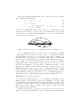
see Figure for an illustration. The resulting problem then calls for a mincost acyclic tournament in G, and is known as the Linear Ordering Problem
(LOP) [3, 4, 5, 13]. Both HP and LOP are known to be NP-hard problems.
Figure 1: Acyclic tournaments are made by an Hamiltonian path (thick
arcs) plus its transitive closure (thin arcs)
In some applications, both the HP and the LOP frameworks are unappropriate to describe the cost function. In this paper we introduce and
study, for the first time, a relevant case arising when the overall permutation
2
cost can be expressed as the sum of terms αu associated with each item u,
each defined as a linear combination of the values αv of all items v that
follow u in the permutation. To be more specific, we address the following
problem:
Definition 1.1 (LOP-CC). Given a complete digraph G = (V, A) with
nonnegative node weights pv and nonnegative arc costs cuv , the Linear Ordering Problem with Cumulative Costs (LOP-CC) is to find an Hamiltonian path P = {(k1 , k2 ), · · · , (kn−1 , kn )} and the corresponding node values
αv that minimize the total cost
π(P ) =
n
X
αv
v=1
under the constraints
αki = p ki +
n
X
cki kj αkj ,
for i = n, n − 1, · · · , 1
(1)
j=i+1
Constraints (1) imply a cumulative “backward propagation” of the value of
variables αv for v = n, n − 1, · · · , 1, hence the name of the problem. We will
also address a constrained version of the same problem, namely:
Definition 1.2 (BLOP-CC). The Bounded Linear Ordering Problem with
Cumulative Costs (BLOP-CC) is defined as the problem LOP-CC above,
plus the additional constraints:
αi ≤ U
∀i ∈ V
(2)
where U is a given nonnegative bound.
Notice that BLOP-CC can be infeasible. As shown in the next section,
BLOP-CC finds important practical applications, in particular, in the optimization of mobile telecommunication systems.
In this paper we introduce and study both problems LOP-CC and BLOPCC. In Section 2, we give the practical application that motivated the present
study and leaded to the patented new methodology for cellular phone management described in [2]. In Section 3, we show that both LOP-CC and
BLOP-CC are NP-hard. A Mixed-Integer linear Programming (MIP) model
is presented in Section 4, whereas an ad-hoc enumerative method is introduced in Section 5. Extensive computational results on a large set of instances are presented in Section 6, whereas some conclusions are drawn in
Section 7.
As G is assumed to be complete, in the sequel we will not distinguish
between an Hamiltonian path P = {(k1 , k2 ), · · · , (kn−1 , kn )} and the associated node permutation K = hk1 , · · · , kn i. Moreover, given any Hamiltonian
3
path P = {(k1 , k2 ), · · · , (kn−1 , kn )}, we call direct all arcs (ki , ki+1 ) ∈ P
(the thick ones in Figure 1), whereas the arcs (ki , kj ) for j ≥ i + 1 are called
transitive (these are precisely the arcs in [P ] \ P , depicted in thin line in
Figure 1). Finally, we use notation π(P ) to denote the cumulative
cost of
Pn
an Hamiltonian path P , defined as the LOP-CC cost π = v=1 αv of the
corresponding permutation.
2
Motivation
In this section we outline the practical problem that motivated the present
paper; the interested reader is referred to [1], [9] and [12] for more details.
In wireless cellular communications, mobile terminals (MTs) communicate simultaneously with a common Base Station (BS). In order to distinguish among the signals of different MTs, the Universal Mobile Telecommunication Standard (UMTS) [15] adopts the so-called code division multiple
access technique, where each terminal is identified by a specific code. Due to
the distortions introduced by radio propagation, the MTs partially interfere
with each other, hence the need to keep the multiuser access interference
below an acceptable level. A very effective technique for interference reduction has been proposed [11], and is called Successive Interference Cancellation (SIC). According to this method, MT signals are detected sequentially
from the received signal, according to a predetermined order. After each
detection, interference is removed from the received signal, thus allowing for
improved detection for the next users.
A crucial problem in the design of the SIC system is therefore the choice
of the detection order. Usually, users are ordered by decreasing received
power [11], although a better performance can be obtained by considering
also the level of mutual interference among users. A second issue is the choice
of the power level αi at which the i-th user has to transmit its data. Indeed,
a large power level typically allows for an improved signal detection, whereas
the minimization of the transmission power yields a longer duration of the
batteries of the MT.1 Moreover, physical and regulatory constraints impose
an upper bound, U , on the transmission power of the mobile terminals.
Both the choice of the cancellation order and of the transmission power
levels must ensure a reliable detection of the signals coming from all MTs.
A proper reception is ensured when the average Signal-to-Noise (plus Interference) power ratio (SNIR) is equal to a target level Γ. For a SIC receiver,
the SNIR is related to the power of the interference generated from user i
on user j, denoted by ρij . In particular, upon detection of user kp the SNIR
is
αkp ρkp kp
P
SN IR(p) =
(3)
√
N0 ρkp kp + i∈Up αi NS ρikp
1
Battery lifetime is one of the main limiting factors for mobile communication systems
4
where N0 (noise power) and NS (spreading factor) are given parameters,
and
Up = {kp+1 , kp+2 , · · · , kn }
(4)
is the set of undetected user at stage p.
One then faces the problem of jointly optimizing the SIC detection order
and the transmission power levels, with the aim of minimizing the overall
transmission power while ensuring a proper reception for all users. This
problem, called joint power-control and receiver optimization (JOPCO), has
been introduced in [1], and can be formalized as follows: given a set of users
{1, 2, . . . , n}, the interference factors ρij (i, j = 1, . . . , n), the noise power
N0 , the spreading factor NS , the target ratio Γ, and the maximum allowed
power level U , find the transmission power levels αi (i = 1, · · · , n) and the
detection permutation
K = hk1 , . . . , kn i that minimize the total transmission
Pn
power π = i=1 αki under the following constraints:
Γ=
αki ρki ki
P
,
√
N0 ρki ki + l∈Ui αl NS ρlki
αi ≤ U
for i = 1, · · · , n
(5)
(6)
In [1] a simple GRASP heuristic is proposed for JOPCO with the aim
of minimizing the system transmit power under the constraint of ensuring
the same quality of the transmission (measured by the average raw Bit Error Rate, BER) to all users. In particular, the requirement on the BER
is translated into a constraint on the SNIR at the detection point of each
user, as discussed before. Extensive experiments are reported, showing that
the JOPCO technique performs much better than the usual Average Power
(AP) approach in all the four scenarios simulated, both in terms of quality of
the transmission (BER) and of allocated transmission power. In particular,
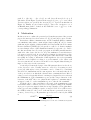
Figure 2 (taken from [1]) illustrates the average BER vs. the number n of
active users for so-called synchronous and asynchronous transmission systems, and compares the JOPCO and AP methodologies. Thin and bold lines
correspond to the case with and without the so-called scrambling operation
on transmitted data, respectively.
It can be seen that, both with and without scrambling, JOPCO ensures
approximately a constant average raw BER of 10−3 up to 10 active users with
respect to the classical AP technique. In the case of syncronous transmission
without scrambling, AP gives a BER that is even lower than the target,
just because it allocates much more transmission power than necessary to
guarantee the target quality, as can be seen in Figure 3 (top). When a larger
number of active users is present, instead, JOPCO has slight performance
degradation due to errors in the interference cancellation.
The JOPCO performance is indeed very good up to 10 active users,
as the average BER is below 10−3 . When a larger number of active users
5
is present, instead, we have a performance degradation due to interference
effects.
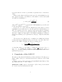
Figure 3 (also taken from [1]) gives the expected total transmission power
ratio expressed in dB, η, as a function of the number of active users (with
and without scrambling), i.e.,
"
#
(AP )
Ptot
η = 10 log10 E
.
(7)
(JOP CO)
Ptot
(AP )
(JOP CO)
where Ptot and Ptot
represent the total transmission power allocated
by AP and JOPCO, respectively.
In all cases, we observe that the JOPCO approach requires a reduced
transmission power with respect to the AP approach. In particular, for a
full loaded synchronous (resp., asynchronous) system without scrambling,
on average the system power requirement using the JOPCO technique is 7
dB (resp., 3 dB) lower than that for AP. When scrambling is considered,
instead, the JOPCO power requirement is 3 dB (resp., 2dB) lower than that
for AP.
We next show how JOPCO can be formulated as a BLOP-CC. Clearly,
for any given user permutation K the power levels αi are univocally determined by the SNIR constraints (5). Indeed, rewriting (5) as
P
√
ΓN0 ρki ki + ΓNS l∈Ui αl ρlki
αki =
ρki ki
one has that values αki can easily be computed in the reverse order i =
√
n, n − 1, · · · , 1. Defining the weights pi = ΓN0 / ρii and the costs cij =
ΓNS ρji /ρii one then obtains precisely the BLOP-CC formulation introduced
in the previous section.
3
Complexity of the LOP-CC
We start proving that the LOP-CC problem is NP-hard. We first give a
simple outline of the proof, and then address in a formal proof the details
required.
Our proof is by reduction from the following Hamiltonian Path problem,
HP, which is known to be NP-complete.
Definition 3.1 (HP). Given a digraph GHP = (VHP , AHP ), decide whether
G contains any directed Hamiltonian path.
6
−1
10
AP
JOPCO
−2
BER
10
−3
10
−4
10
2
4
6
8
10
number of active users
12
14
16
4
6
8
10
number of active users
12
14
16
−1
10
AP
JOPCO
−2
BER
10
−3
10
−4
10
2
Figure 2: The average raw bit error rate BER vs. the number of active
users for synchronous (top) and asynchronous (bottom) transmissions, with
scrambling (thin line) and without scrambling (bold line)
7
8
η
AP/JOPCO
7
6
η [dB]
5
4
3
2
1
0
0
2
4
6
8
10
number of active users
12
14
16
12
14
16
3
η
AP/JOPCO
2.5
η [dB]
2
1.5
1
0.5
0
0
2
4
6
8
10
number of active users
Figure 3: The expected total transmission power ratio η vs. the number of
active users for synchronous (top) and asynchronous (bottom) transmissions,
with scrambling (thin line) and without scrambling (bold line)
8
Our reduction takes any HP instance GHP = (VHP , AHP ) and computes
the following LOP-CC instance:
V
:= VHP = {1, · · · , n}
(8)
pi := 1 ∀i ∈ V
½
M if (i, j) ∈ AHP
cij =
2M otherwise
(9)
∀i, j ∈ V, i 6= j
(10)
where M is a sufficiently large positive value (to be defined later). The
construction can clearly be carried out in polynomial time, provided that
value M can be stored in a polynomial number of bits a property that will
be asserted in the formal proof.
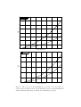
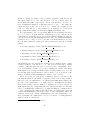
Figure 4: The worst-case “good” path used in the complexity proof
“Good” Hamiltonian paths of G (i.e., those corresponding to Hamiltonian paths in GHP ) only involve direct arcs of cost equal to M , while
all the transitive arcs have a cost not larger than 2M ; see Figure 4 for
an illustration. It is therefore not difficult to show that, for sufficiently
large M , the overall cumulative cost associated with such a path is π(P ) =
M n−1 + O(M n−2 ). On the other hand, if P does not correspond to a Hamiltonian path in GHP , then it has to involve at least one direct arc of cost
2M , hence its cumulative cost π(P ) cannot be smaller than 2M n−1 . For a
large M , our construction then ensures that π(P ) < π(P 0 ) for any “good”
Hamiltonian path P and for any “non-good” Hamiltonian path P 0 , which
implies that GHP contains an Hamiltonian path if and only if any arbitrary
optimal LOP-CC solution corresponds to a “good” Hamiltonian path (or,
equivalently, if the optimal LOP-CC value is strictly less than 2M n−1 ).
Theorem 3.1. LOP-CC is NP-hard
Proof. Given the transformation above, our formal proof amounts to establishing an upper bound U Bgood (n, M ) on the cumulative cost π(P ) of any
“good” Hamiltonian path P as well as a lower bound LBnogood (n, M ) on the
cumulative cost π(P 0 ) of any “non-good” Hamiltonian path P 0 , and to show
that U Bgood (n, M ) < LBnogood (n, M ) for all n and for a value of M such
that log(M ) is polynomial in n.
The lower bound LBnogood (n, M ) corresponds to the case where only one
direct arc in P 0 has cost 2M , hence it can be computed in a straightforward
9
way as
LBgood (n, M ) = 2M n−1
(11)
As to upper bound U Bgood (n, M ), it is computed by considering the
cumulative cost of a Hamiltonian path P where all direct arcs have cost M ,
whereas all transitive arcs have cost 2M . This case is illustrated in Figure 4.
To be more precise, we claim that
π(Pn ) ≤ U Bgood (n, M ) := M n−1 + 4n M n−2
(12)
holds for any Hamiltonian path Pn in G whose direct arcs all have cost
M , where M > 1 is assumed. The proof of this claim is by induction
on n. The claim clearly holds in cases n = 1 and n = 2, where we have
π(P1 ) = 1 and π(P2 ) = M + 2, respectively. We assume now that (12)
holds for all n ≤ h for a given h ≥ 2, and we prove that it also holds for
n = h + 1. Let Pn=h+1 = {(k1 , k2 ), · · · , (kh , kh+1 )} be any Hamiltonian path
whose direct arcs all have cost M , and let Ph = {(k2 , k3 ), · · · , (kh , kh+1 } and
Ph−1 = {(k3 , k4 ), · · · , (kh , kh+1 } be obtained from Ph+1 by removing its first
arc and its first two arcs, respectively. We have
π(Ph+1 ) =
h+1
X
i=1
αki =
h+1
X
αki + αk1
i=2
= π(Ph ) + αk1
≤ π(Ph ) + M αk2 + 1 + 2M
h+1
X
αki
(because of (1) and (10))
i=3
≤ π(Ph ) + M π(Ph ) (since π(Ph ) ≥ αk2 + 1)
P
+ 2M π(Ph−1 ) (since π(Ph−1 ) = h+1
i=3 αki )
≤ (1 + M )π(Ph ) + 2M π(Ph−1 )
The claim then follows from the induction hypothesis, as we have
π(Ph+1 ) ≤ (1 + M )(M h−1 + 4h M h−2 ) + 2M (M h−2 + 4h−1 M h−3 )
3
≤ M h + (3 + 4h )M h−1 + 4h M h−2
(13)
2
5
(14)
≤ M h + (3 + 4h )M h−1 (since M h−2 ≤ M h−1 )
2
≤ M h + 4h+1 M h−1 (since h ≥ 2)
(15)
To complete the complexity proof, we have to choose a value for M that
guarantees U Bgood (n, M ) < LBnogood (n, M ), i.e.,
M n−1 + 4n M n−2 < 2M n−1 =⇒ 4n M n−2 < M n−1 =⇒ 4n < M
We then set M = 4n + 1, whose size log(M ) = O(n) is polynomial in n, as
required.
10
Corollary 3.1.1. BLOP-CC is NP-hard
Proof. We use the same construction as in the proof of the previous theorem,
2
with U := U Bgood (n, M ) = O(M n ) = O(4n ) large enough to make all
“good” Hamiltonian paths in G feasible for the BLOP-CC instance, but
still with size log(U ) = O(n2 ).
4
A MIP model
In this section we introduce a MIP model for BLOP-CC, derived from the
LOP model of Grötschel, Jünger and Reinelt [3].
As already mentioned, in a standard linear ordering problem we have n
items to be placed in a convenient order. If we place item i before item j, we
pay a cost of gij . The objective is to choose the item order that minimizes
the total cost. This problem can then be modelled as
P
min
(i,j)∈A gij xij
subject to “x is the incidence vector of an acyclic tournment”
where xij = 1 if item i is placed before j in the final order, xij = 0 otherwise.
In order to get an acyclic tournament, it is shown in [3] that, besides the
obvious conditions
xij + xji = 1,
∀(i, j) ∈ A, i < j
(16)
it is sufficient to prevent 3-node cycles of the form xij = xjk = xki = 1,
leading to the triangle inequalities
xij + xjk + xki ≤ 2
(17)
Using the same set of variables, one can rewrite the LOP-CC constraints
(1) as the nonlinear equalities:
αi = p i +
n
X
cij αj xij
∀i ∈ V
(18)
j=1
In order to get linear constraints, we introduce the following n(n − 1)
new variables:
½
αj if xij = 1
yij (= αj xij ) =
∀i, j ∈ V : i 6= j
(19)
0 otherwise
Thus (18) becomes linear in the y variables,
αi = p i +
n
X
j=1
11
cij yij
and conditions (19) become
xij = 0 ⇒ yij = 0
xij = 1 ⇒ yij ≥ αj
xij = 1 ⇒ yij ≤ αj
−→ yij ≤ M xij
−→ yij ≥ αj − M (1 − xij )
−→ yij ≤ αj + M (1 − xij )
where M is a sufficiently large positive value. Notice that constraints yij ≤
αj + M (1 − xij ) can be removed from the model, as the minimization of
variables αj implies that of variables yij . (As to constraints yij ≤ M xij ,
they are redundant as well; however, our computational experience showed
that they improve the numerical stability of the MIP solver, so we keep
them into our model.) Also, from (19), the y variables are bounded by the
α variables, thus we can take M = U . Finally, α ≥ 0 can be assumed since
p, c ≥ 0).
As it is customary in LOP models, one can use equations (16) to eliminate all variables xij with i > j,2 and modify the triangle inequalities into:
xij + xjk − xik ≤ 1
for all 1 ≤ i < j < k ≤ n
−xij − xjk + xik ≤ 0 for all 1 ≤ i < j < k ≤ n
This leads to the following MIP model for BLOP-CC:
Pn
minimize
i=1 αi
subject to xij + xjk − xik ≤ 1
for 1 ≤ i < j < k ≤ n
xij + xjk −
x
≥
0
for
1≤i<j<k≤n
Pnik
αi = pi + j=1 cij yij
for 1 ≤ i ≤ n
yij ≤ U xij
for 1 ≤ i < j ≤ n
yji ≤ U (1 − xij )
for 1 ≤ i < j ≤ n
yij ≥ αj − U (1 − xij )
for 1 ≤ i < j ≤ n
yji ≥ αi − U xij
for 1 ≤ i < j ≤ n
0 ≤ αi ≤ U
for 1 ≤ i ≤ n
yij ≥ 0
for 1 ≤ i 6= j ≤ n
xij ∈ {0, 1}
for 1 ≤ i < j ≤ n
5
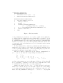
An ad-hoc enumerative algorithm
Our enumerative algorithm is based on a standard backtracking technique
(akin to those used in Constraint Programming) to generate all permutations and to find one with the lowest total cost. To limit the number of
permutations actually evaluated, we use a pruning mechanism based on
lower bounds.
Permutations are built progressively, and are extended backwards from
the last node. At the root of the search tree (depth 0), none of the permutation elements in K = hk1 , · · · , kn i is fixed. At depth 1, the last element
2
The α variables could be removed as well, but this would have a marginal effect on
the solution time of the model.
12
Permutation generation:
TraverseSearchTree(n)
1.
initialize set S := {1, 2, · · · , n}
2.
EnumeratePermutationElement(n)
EnumeratePermutationElement(i)
3.
for each element e in S do
4.
remove e from S
5.
perm[i] ← e
6.
evaluate partial permutation
h∗, · · · , ∗, perm[i], perm[i + 1],· · · ,perm[n]i
7.
if i > 1 then EnumeratePermutationElement(i − 1)
8.
insert e back into S
9.
enddo
Figure 5: The basic method
of the permutation, kn , is fixed to one of the n possible choices (thus, the
root has n sons). At depth 2, the next to last item, kn−1 , is fixed to one of
the remaining n − 1 possible choices, and so on. The search tree is visited
in depth-first manner. The only required data structures to implement this
method are an array to store the current partial permutation, and another
to keep track of the nodes that have not yet been inserted in the current
partial permutation.
We chose this method to enumerate permutations, rather than more sophisticated ones, because we can compute very quickly a parametric lower
bound for partial permutations (to be used for pruning purposes), thus enumerating very effectively a large number of nodes.
Our lower bound is computed as follows. Given a permutation K =
hk1 , · · · , kn i, we can write the corresponding node values αv as:
αkn
αkn−1
αkn−2
···
= pkn
= pkn−1
= pkn−2
+ αkn
+ αkn
ckn−1 ,kn
ckn−2 ,kn
+ αkn−1
ckn−2 ,kn−1
and the total permutation cost π is the sum of all the αv . Notice that all
the node weights pv contribute to the total cost, so their sum can be used
as an initial lower bound for the cost of any permutation.
Assume now that nodes ki+1 , ki+2 , · · · , kn have already been chosen.
When node ki is also chosen, one can easily compute the corresponding
αki by using equation (1). Furthermore, the contribution of this αki to the
final cost of any permutation of the type h∗, · · · , ∗, ki , ki+1 , · · · , kn i is given
13
by:
αki
X
cuki
(20)
u∈{k
/ i ,··· ,kn }
regardless of the rank of the remaining nodes in the complete permutation.
This property allows us to compute easily, in a parametric way, a valid lower
bound on the cost of any such permutation.
To be more specific, our
P pruning mechanism works as follows. We start
with lower bound LB := v pv and with an empty permutation. We then
build-up partial permutations recursively. Every time a new node ki is
inserted in front of the current permutation, we compute the corresponding
αki and add (20) to the current lower bound LB. If the resulting LB is
strictly smaller than the incumbent solution value, we proceed with the
recursion; otherwise we backtrack, and update LB accordingly.
A small modification of this algorithm can be used to start with a
given permutation (rather than from scratch), thus allowing the enumerative search to quickly produce improved permutations through successive
modifications of the starting one. To this end, the only change required at
Step 3 of the algorithm of Figure 5 is to implement the set S as a FIFO
queue, to be initialized with the desired starting permutation (the last node
in the sequence being the first to be extracted).
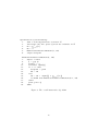
In our implementation we use a simple yet effective heuristic to find a
“good” initial solution for the BLOP-CC instances arising in our telecommunication application. Namely, we sort the nodes by decreasing autocorrelation factors ρii , and consider the associated permutation (the first and
last node in the permutation being those with the largest and smallest ρii ,
respectively) to initialize our incumbent solution. Alternative heuristics to
find a good initial permutation are presented in [1].
Our complete algorithm is outlined in Figure 6.
6
Computational results
We have compared the performance of our enumerative algorithm with that
of a state-of-the-art commercial MIP solver (ILOG-Cplex 9.0.2 [7]) applied
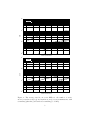
to the MIP model of Section 4. The outcome of this experiment is reported
in Table 1, where 4 large sets of BLOP-CC instances have been considered.
The instances used in our study have been provided by the telecommunications group of the Engineering School of the University of Padova,
and are related to detection-order optimization in UMTS networks [1]. All
the four communication scenarios considered in [1] have been addressed:
synchronous and asynchronous transmission, with and without scrambling.
For each scenario, 500 matrices (ρij ) have been randomly generated assuming the presence of 16 users3 uniformly distributed in the cell (with a
3
The UMTS technology considers up to 8-16 active users at a time; a larger number of
14
Optimization by backtracking:
1.
find a starting heuristic solution H
2.
initialize
the fifo queue Q with the elements in H
P
3.
LB ← ni=1 p[i]
4.
UB ← ∞
5.
EnumeratePermutationElement(n, LB)
6.
output bestperm
EnumeratePermutationElement(i, LB)
7.
repeat i times
8.
q ← pop Q
9.
perm[i] ← q
10.
calculate alpha[q]
11.
if i = 1 then
12.
bestperm ← perm
13.
UB ← LB
14.
else
P
15.
LB ← LB + alpha[q] *
r∈Q c[r,q]
16.
if LB<UB then EnumeratePermutationElement(i-1, LB)
17.
endif
18.
push q into Q
19.
enddo
Figure 6: The overall enumerative algorithm
15
radius of 580 m), according to the so-called log-distance path loss model.
The input values Γ, U , NS , and N0 have been set to 0.625, 10.0, 16,
and 0.50476587558415, respectively. From each matrix ρ, we have derived 8 BLOP-CC instances of different sizes (n = 2, 4, . . . , 16), using the
equations given at the end of Section 2 to compute the weights pv and
costs cuv . The full set of these matrices ρ is available for download at
http://www.math.unipd.it/~bertacco/LOPCC_instances.zip
For each instance, the corresponding MIP model is built-up through a
C++ code based on ILOG Concert Technology 2.0 [8]. All the model
constraints are statically incorporated in the initial formulation, and the
outcome is solved through ILOG-Cplex 9.0.2. Since the default ILOG-Cplex
tolerances are too large to solve correctly even small instances, we used
the following parameter setting (all other parameters being left at default
values):
• Absolute mipgap tolerance (CPX PARAM EPAGAP): 1e-13
• Relative mipgap tolerance (CPX PARAM EPGAP): 1e-11
• Integrality tolerance (CPX PARAM EPINT): 1e-9
• Optimality tolerance (CPX PARAM EPOPT): 1e-9
• Feasibility tolerance (CPX PARAM EPRHS): 1e-9
Unfortunately, in some cases these tolerances are not small enough to ensure
a valid resolution, even when n = 2. The reason is that the ρ matrix
contains coefficients that may vary by several orders of magnitude, hence
even our feasibility tolerance of 1e-9 can be insufficient. On the other hand,
ILOG-Cplex does not support smaller values for this parameter, so we could
not fix this pathological situation, and we had to report in Table 1 the
number of instances that ILOG-Cplex could not solve correctly.
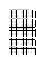
Table 1 reports, for each group of instances and for each size n, the
following information: the number of instances solved, the average solution
times for both our enumerative code (Enum) and ILOG-Cplex (MIP ), the
speedup of the enumerative code with respect to ILOG-Cplex, the maximum solution times, and the number of instances not solved correctly by
ILOG-Cplex (# fails). Computing times are expressed in CPU seconds, and
refer to a Pentium M 1.4 Ghz notebook with 512 MBytes of main memory.
The computational results clearly show that our enumerative approach
outperforms ILOG-Cplex, and is up to three orders of magnitude faster. As
a matter of fact, in no instance ILOG-Cplex beated the enumerative code.
As to scalability, the enumerative code proved capable of solving instances
with n = 20 in about 4 hours.
active users is unrealistic for this application
16
Set 1: Synchronous communication without scrambling
size
2
4
6
8
10
12
14
16
# instances
Enum MIP
500
500
500
500
500
500
500
500
500
500
500
500
500
50
500
5
average time (sec.s)
Enum
MIP
0.0
0.0
0.0
0.0
0.0
0.5
0.0
9.6
0.2
395.0
4.8
22,233.0
Enum
speedup
497
186
787
1,906
4,574
max time (sec.s)
Enum
MIP
0.0
0.0
0.0
0.0
0.0
0.0
0.6
0.0
5.3
0.2
455.5
12.5
2,537.6
381.9 60,096.2
# fails
2
2
7
7
6
9
1
1
Set 2: Synchronous communication with scrambling
size
2
4
6
8
10
12
14
16
# instances
Enum MIP
500
500
500
500
500
500
500
500
500
500
500
500
500
50
500
4
average time (sec.s)
Enum
MIP
0.0
0.0
0.0
0.0
0.0
0.6
0.0
8.8
0.5
267.4
15.0
14,473.2
Enum
speedup
237
441
503
964
max time (sec.s)
Enum
MIP
0.0
0.0
0.0
0.0
1.0
0.0
10.0
0.9
319.8
43.1
2,256.9
794.6 49,424.0
# fails
3
5
8
7
7
10
1
1
Set 3: Asynchronous communication without scrambling
size
2
4
6
8
10
12
14
16
# instances
Enum MIP
500
500
500
500
500
500
500
500
500
500
500
500
500
50
500
5
average time (sec.s)
Enum
MIP
0.0
0.0
0.0
0.1
0.0
1.2
0.0
30.0
0.2
1,130.8
5.6
28,191.6
Enum
speedup
1,212
2,447
5,218
4,978
max time (sec.s)
Enum
MIP
0.0
0.0
0.0
0.0
0.5
0.0
13.1
0.2
786.6
11.9
8,058.2
407.8 61,402.8
# fails
2
3
6
4
4
10
0
1
Set 4: Asynchronous communication with scrambling
size
2
4
6
8
10
12
14
16
# instances
Enum MIP
500
500
500
500
500
500
500
500
500
500
500
500
500
50
500
2
Overall statistics
size
2
4
6
8
10
12
14
16
# instances
Enum MIP
2000 2000
2000 2000
2000 2000
2000 2000
2000 2000
2000 2000
2000
200
2000
16
average time (sec.s)
Enum
MIP
0.0
0.0
0.0
0.1
0.0
1.3
0.0
31.3
0.2
1,801.5
6.3
8,362.0
Enum
speedup
1,096
2,310
6,880
1,316
max time (sec.s)
Enum
MIP
0.0
0.0
0.0
0.0
0.0
0.0
0.0
0.7
0.0
15.8
0.2
473.4
6.6 35,469.5
204.8
9,821.5
# fails
3
2
3
4
4
8
1
1
average time (sec.s)
Enum
Enum
MIP speedup
0.0
0.0
0.0
0.1
1,146
0.0
0.9
488
0.0
20.0
1,373
0.3
898.7
2,952
7.9
20,421.217
2,562
max time (sec.s)
Enum
MIP
0.0
0.0
0.0
0.0
0.0
0.0
0.0
1.0
0.0
15.8
0.9
786.6
43.1 35,469.5
794.6 61,402.8
# fails
10
12
24
22
21
37
3
4
Table 1: Computational results
All the instances in our testbed were solved to proven optimality, thus
enabling us to benchmark the GRASP heuristic proposed in [1] (evaluating
the performance of this method was indeed our initial motivation in studying
BLOP-CC).
7
Conclusions
We have introduced and studied, for the first time, a new optimization
problem related to the well-known Linear Ordering Problem, in which the
solution cost is non-linear due to a cumulative backwards propagation mechanism. This model was motivated by a practical application in UMTS
mobile-phone telecommunication system.
We have formalized the problem, in two versions, and proved that they
are both NP-hard. We have proposed a Mixed-Integer Linear Programming
model as well as an ad-hoc enumerative algorithm for the exact solution
of the problem. Extensive computational results on large sets of instances
have been presented, showing that the proposed techniques are capable of
solving, in reasonable computing times, all the instances coming from our
application. As a byproduct, our method allowed to benchmark the GRASP
heuristic proposed in [1].
Future research should be devoted to enhancing the MIP formulation,
and/or to embed more sophisticated pruning mechanisms in our enumerative
scheme. Also worth studying are more complex (nonlinear) cost functions
applied to the basic Linear Ordering model.
Acknowledgements
Work supported by MIUR and CNR, Italy. Thanks are due to Nevio
Benvenuto, Giambattista Carnevale, and Stefano Tomasin for helpful discussions on the JOPCO methodology.
References
[1] N. Benvenuto, G. Carnevale and S. Tomasin. Joint Power Control and
Receiver Optimization of CDMA Transceivers using Successive Interference Cancelation. Technical Report DEI, Department of Information
Engineering, University of Padova (2004).
[2] N. Benvenuto and S. Tomasin. On the Comparison Between OFDM
and Single Carrier Modulation With a DFE Using a Frequency-Domain
Feedforward Filter. IEEE Transactions on Communications 50(6), 947955, 2002.
18
[3] M. Grötschel, M. Jünger, and G. Reinelt. A Cutting Plane Algorithm
for the Linear Ordering Problem. Operations Research, 32, 1195-1220,
1984.
[4] M. Grötschel, M. Jünger, and G. Reinelt. On the acyclic subgraph
polytope. Mathematical Programming, 33, 28-42, 1985.
[5] M. Grötschel, M. Jünger, and G. Reinelt. Facets of the Linear Ordering
Polytope. Mathematical Programming, 33, 43-60, 1985.
[6] G. Gutin and A. Punnen (editors) The Traveling Salesman Problem
and its Variations, Kluwer, 2002.
[7] ILOG Cplex 9.0: User’s Manual and Reference Manual, ILOG, S.A.,
http://www.ilog.com/, 2004.
[8] ILOG Concert Technology 2.0: User’s Manual and Reference Manual,
ILOG, S.A., http://www.ilog.com/, 2004.
[9] H. Holma and A. Toskala. WCDMA for UMTS: Radio Access for Third
Generation Mobile Communications, Wiley, New York, 2000.
[10] J.K. Lenstra, A.H.G. Rinnooy Kan and D.Shmoys (editors). The Traveling Salesman Problem: A Guided Tour to Combinatorial Optimization, Wiley, 251-305, 1985.
[11] P. Patel and J. Holzman. Analysis of a Simple Successive Interference
Cancellation Scheme in a DS/CDMA System. IEEE J. Select. Areas
Commun., 12, 727–807, 1994.
[12] J. G. Proakis. Digital Communications 4th edition, McGraw Hill, New
York, 2004
[13] G. Reinelt. The Linear Ordering Problem: Algorithms and Applications. Research and Exposition in Mathematics 8, Heldermann Verlag,
Berlin, 1985
[14] D. Warrier and U. Madhow. On the Capacity of Cellular CDMA with
Successive Decoding and Controlled Power Disparities. in Proc. Vehic.
Tech. Conf. (VTC), vol. 3, 1873–1877, 1998.
[15] 3GPP, Technical Specification Group Radio Access Networks; Radio
Transmission and Reception. 3G TS 25.102 version 3.6.0, 1999.
19