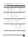
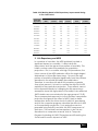
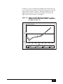
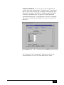
1
Table of Contents I. INTRODUCTION......................................................................................................... 1 A. Description of the Spectrum System............................................................. 1 1. Components .................................................................................................... 1 2. Software Description....................................................................................... 2 B. Uses of Spectrum Policy Models ................................................................... 2 C. Organization of the Model Manuals............................................................. 4 D. Information about the POLICY Project ......................................................... 4 E. What Is DemProj?............................................................................................ 5 F. Why Make Population Projections?.............................................................. 6 II. STEPS IN MAKING A POPULATION PROJECTION .................................................... 7 III. DEMOGRAPHIC INPUTS AND OUTPUTS.................................................................... 9 A. Base Year Population................................................................................... 10 B. Fertility ........................................................................................................... 12 1. The Total Fertility Rate ................................................................................ 12 Base Year Estimates..................................................................................................... 12 Future Assumptions ...................................................................................................... 13 2. The Age Distribution of Fertility ................................................................. 16 Use of Fertility Models in Population Projections................................................... 16 Fertility Surveys.............................................................................................................. 17 Regionality and Model Fertility Patterns: the United Nations Model Schedules ...................................................................................................................... 20 Combining Data from Fertility Surveys with Model Tables.................................. 23 The Coale-Trussell Fertility Model .............................................................................. 23 C. Mortality ........................................................................................................ 25 1. Life Expectancy at Birth ............................................................................ 25 Base Year Estimates..................................................................................................... 25 Future Assumptions ...................................................................................................... 25 2. Life Expectancy and AIDS ........................................................................ 27 iii 3. Age-Specific Mortality ............................................................................... 28 Model Mortality Tables................................................................................................ 28 Regional Model Life Tables........................................................................................ 29 Selecting a Model Life Table..................................................................................... 32 Modifying the Model Life Tables............................................................................... 33 D. Migration ....................................................................................................... 34 E. Current Population: Urban and Rural......................................................... 35 F. Projection Outputs........................................................................................ 37 IV. PROGRAM TUTORIAL .............................................................................................. 39 A. Before You Get Started ................................................................................ 39 B. Installing the Spectrum Program................................................................. 40 C. Creating a New Projection .......................................................................... 40 1. Starting the Spectrum Program............................................................... 40 2. Specifying the Projection Parameters in Projection Manager ......... 41 D. Entering the Base Year Data and Projection Assumptions....................... 43 1. Specifying New Demographic Projection Parameters...................... 43 2. Entering the Base Year Data and Projection Assumptions ............... 45 3. About the Editors ........................................................................................ 46 First Year Population.................................................................................................... 47 Total Fertility Rate......................................................................................................... 48 ASFR 49 Sex Ratio at Birth .......................................................................................................... 54 Life Expectancy............................................................................................................ 55 Model Life Table........................................................................................................... 57 International Migration............................................................................................... 58 Regional Assumptions ................................................................................................. 58 4. Leaving the Demographic Data Editors ............................................... 59 5. Saving the Input Data ............................................................................... 59 E. Making the Projection.................................................................................. 59 F. Examining the Output .................................................................................. 60 1. Graphs and Bar Charts ............................................................................. 63 2. Tables ............................................................................................................ 63 3. Displaying All Age Groups ........................................................................ 63 4. Demographic Summary Table ................................................................ 64 iv G. Saving the Projection ................................................................................... 64 H. Opening an Existing Projection................................................................... 65 I. Closing a Projection..................................................................................... 65 J. Using DemProj Projections with the Excel Version of RAPID..................... 66 K. Importing a Demographic Projection Produced with an Earlier Version of DemProj....................................................................................... 66 L. Aggregating projections ............................................................................. 67 V. METHODOLOGY ..................................................................................................... 69 A. Calculating the Base Population by Single Ages...................................... 69 B. Survival Ratios ............................................................................................... 71 C. Migration ....................................................................................................... 71 D. Deaths ........................................................................................................... 71 E. Population Size ............................................................................................. 72 F. Births............................................................................................................... 73 G. Urban and Rural Projections........................................................................ 75 VI. REFERENCES ......................................................................................................... 77 VII. GLOSSARY OF TERMS........................................................................................... 79 VIII. ACRONYMS AND ABBREVIATIONS ..................................................................... 85 APPENDIX A: THE COALE-TRUSSELL RELATIONAL FERTILITY MODEL.........................A.1 A.1 Description of the Model..........................................................................A.1 A.2 Employment of the Model in Projections................................................A.3 A.3 An Application to Bangladesh ................................................................A.5 v List of Figures Figure 1: Figure 2: Figure 3: Figure 4: Figure 5: Figure 6: Figure 7: Shift in Fertility Distributions - Bangladesh: 1975 to 1993-94.........................................................18 Shift in Fertility Distributions - Taiwan: 1956 to 1983 ........................................................................18 Fertility Distribution by TFR: UN Sub-Saharan Africa Pattern .......................................................20 Comparison of Model Fertility Tables at a TFR of 4.0.....................................................................21 Shift in Fertility Distributions – Bangladesh and UN Asia Pattern ................................................22 Shift in Fertility Distributions – Bangladesh and UN Sub-Saharan Africa Pattern....................22 ASFRs Generated by Coale-Trussell Model Compared with Survey ASFRs: Bangladesh, BFS 1975..........................................................................................................................24 Figure 8: ASFRs Generated by Coale-Trussell Model Compared with Survey ASFRs: Bangladesh, BFS 1989..........................................................................................................................24 Figure 9: Model Life Table Mortality Probabilities – Coale-Demeny West Female Models Table: Compared by Level of Life Expectancy .........................................................................................30 Figure 10: Model Life Table Mortality Probabilities – Coale-Demeny Female Model Table Families: Comparison by Family at e(0) = 45 ..................................................................................31 Figure 11: Model Life Table Mortality Probabilities – United Nations Female Model Table Families: Comparison by Family at e(0) = 45 ..................................................................................32 Figure 12: Typical Pattern of Urbanization.......................................................................................................36 Figure 13: Fertility Distribution by TFR: UN Sub-Saharan Africa Pattern ....................................................73 Figure 14: Fertility Distribution by TFR: UN Arab Pattern...............................................................................74 Figure 15: Fertility Distribution by TFR: UN Asia Pattern ................................................................................74 Figure A.1: ASFRs Generated by Coale-Trussell Model Compared with Survey ASFRs: Bangladesh, BFS 1975........................................................................................................................ A.6 Figure A.2: ASFRs Generated by Coale-Trussell Model Compared with Survey ASFRs: Bangladesh, BFS 1989......................................................................................................................... A.6 List of Tables Table 1: Declines in TFR in 1990s by Level of Program Effort During 1994-1999 and Socioeconomic Setting.......................................................................................................................15 Table 2. Calculation of the Distribution of Fertility by Age Group from Age-Specific Fertility Rates ........................................................................................................................................................17 Table 3: UN Model Tables of the Age Distribution of Fertility.......................................................................19 Table 4: UN Working Model of Life Expectancy Improvement During a Five-Year Period ..................27 Table A.1: Coale-Trussell Fertility Control Schedule (vx).............................................................................. A.4 Table A.2: Bangladesh: ASFRs from Various Surveys, and Projected Rates............................................ A.7 vi I. Introduction A. Description of the Spectrum System 1. Components POLICY and its predecessor projects have developed computer models that analyze existing information to determine the future consequences of today’s development programs and policies. The Spectrum Policy Modeling System consolidates previous models into an integrated package containing the following components: Spectrum consolidates DemProj, FamPlan, BenefitCost, AIM, and RAPID, NewGen, and PMTCT models into an integrated package. • Demography (DemProj) – A program to make population projections based on (1) the current population, and (2) fertility, mortality, and migration rates for a country or region. • Family Planning (FamPlan) – A program to project family planning requirements in order to achieve national goals for meeting couples’ fertility intentions. • Benefit-Cost – A program for comparing the costs of implementing family planning programs, to the benefits generated by those programs. • AIDS (AIDS Impact Model – AIM) – A program to project the consequences of the AIDS epidemic including the number of people infected with HIV, AIDS deaths, the number of people needing treatment and the number of orphans. Socioeconomic Impacts of High Fertility and Population Growth (RAPID) – A program to project the social and economic consequences of high fertility and rapid population growth for sectors such as labor force, education, health, urbanization and agriculture. • • Adolescent reproductive health (NewGen) – A program to estimate the consequences of adolescent reproductive health behavior, including sexual debut, marriage, pregnancy, abortion, and HIV/STI infection. • Prevention of mother-to-child transmission (PMTCT) – A program to examine the costs and benefits of interventions to prevent the transmission of HIV from 1 mother to child, including anti-retroviral treatment, infant feeding options and delivery options. 2. Software Description Spectrum is a Windows-based system of integrated policy models. The integration is based on DemProj, which is used to create the population projections that support many of the calculations in the other components, such as FamPlan, Benefit-Cost, AIM, and RAPID. Each component has a similarly functioning interface that is easy to learn and to use. With little guidance, anyone who has a basic familiarity with Windows software will be able to navigate the models to create population projections and to estimate resource and infrastructure requirements. The accompanying manuals contain both the instructions for users, and equations for those who want to know exactly how the underlying calculations are computed. B. Uses of Spectrum Policy Models Policy models are designed to answer a number of “what if” questions. The “what if” refers to factors that can be changed or influenced by public policy. Policy models are designed to answer a number of “what if” questions relevant to entities as small as local providers of primary health care services and as large as international development assistance agencies. The “what if” refers to factors that can be changed or influenced by public policy. Models are commonly computerized when analysts need to see the likely result of two or more forces that might be brought to bear on an outcome, such as a population’s illness level or its degree of urbanization. Whenever at least three variables are involved (such as two forces and one outcome), a computerized model can both reduce the burden of manipulating those variables and present the results in an accessible way. Some of the policy issues commonly addressed by the Spectrum set of models include: 2 • The utility of taking actions earlier rather than later. Modeling shows that little in a country stands still while policy decisions are stalled and that many negative outcomes can accumulate during a period of policy stasis. • The evaluation of the costs vs. the benefits of a course of action. Modeling can show the economic efficiency of a set of actions (i.e., whether certain outcomes are achieved more effectively than under a different set of actions), or simply whether the cost of a single set of actions is acceptable for the benefits gained. A set of policies under consideration may not be acceptable to all stakeholders. • The recognition of inter-relatedness. Modeling can show how making a change in one area of population dynamics (such as migration rates) may necessitate changes in a number of other areas (such as marriage rates, timing of childbearing, etc.). • The need to discard monolithic explanations and policy initiatives. Modeling can demonstrate that simplistic explanations may bear little relationship to how the “real world” operates. • The utility of “door openers.” A set of policies under consideration may not be acceptable to all stakeholders. Modeling can concentrate on favored goals and objectives and demonstrate how they are assisted by the proposed policies. • That few things in life operate in a linear fashion. A straight line rarely describes social or physical behavior. Most particularly, population growth, being exponential, is so far from linear that its results are startling. Modeling shows that all social sectors based on the size of population groups are heavily influenced by the exponential nature of growth over time. • That a population’s composition greatly influences its needs and its well being. How a population is composed—in terms of its age and sex distribution— has broad-ranging consequences for social welfare, crime rates, disease transmission, political stability, etc. Modeling demonstrates the degree to which a change in age and sex distribution can affect a range of social indicators. • The effort required to “swim against the current.” A number of factors can make the success of a particular program harder to achieve; for example, the waning of breastfeeding in a population increases the need for contraceptive coverage. Modeling can illustrate the need for extra effort—even if simply to keep running in place. 3 C. Organization of the Model Manuals Each manual begins with a discussion of what the model does and why someone would want to use it. The manual also explains the data decisions and assumptions needed before the model can be run, and possible sources for the data. It defines the data inputs and outputs. The manual contains a tutorial, information on the methodology behind the model, a glossary, and a bibliography. D. Information about the POLICY Project The POLICY Project is a USAID-funded activity designed to create a supportive environment for family planning and reproductive health programs through the promotion of a participatory process and population policies that respond to client needs. To achieve its purpose, the project addresses the full range of policies that support the expansion of family planning and other reproductive health services, including: The POLICY Project is implemented by the Futures Group in collaboration with Research Triangle Institute (RTI) and the Centre for Development and Population Activities (CEDPA). • national policies as expressed in laws and in official statements and documents; • operational policies that govern the provision of services; • policies affecting gender roles and the status of women; and • policies in related sectors, such as health, education and the environment that affect populations. More information about the Spectrum System of Policy Models and the POLICY Project are available from: Director, POLICY Project Futures Group One Thomas Circle, NW Suite 200 Washington, DC 20005 U.S.A. Telephone: (202) 775-9680 Fax: (202) 775-9694 E-mail: [email protected] http://www.FuturesGroup.com or The POLICY Project U.S. Agency for International Development Center for Population, Health, and Nutrition 1300 Pennsylvania Ave. Washington, DC 20523 U.S.A. Telephone: (202) 712-5787 or -5839 4 E. What Is DemProj? The demographic model in Spectrum, known as DemProj, is a computer program for making population projections for countries or regions. The program requires information on the number of people by age and sex in the base year, as well as current year data and future assumptions about the total fertility rate (TFR), the age distribution of fertility, life expectancy at birth by sex, the most appropriate model life table, and the magnitude and pattern of international migration (all of these inputs are discussed in Chapter III). This information is used to project the size of the future population by age and sex for as many as 150 years into the future. If desired, the projection can also estimate the size of the urban and rural populations. Linking DemProj with other modules in Spectrum makes it possible to examine the demographic impact of AIDS (AIM), the family planning service requirements to achieve demographic and health goals (FamPlan), the costs and benefits of family planning programs and the socioeconomic impacts of high fertility and rapid population growth (RAPID). DemProj was first produced in 1980. Since then, it has been used by a large number of planners and researchers around the world. It has been updated from time to time in response to comments and suggestions from users. This current release, DemProj 4, incorporates a number of new features in response to these comments. DemProj is designed to produce information useful for policy formulation and dialogue within a framework of easy-to-use computer programs. DemProj (and the entire Spectrum system) is designed to produce information useful for policy formulation and dialogue within a framework of easy-to-use computer programs. The focus is on the generation of information useful for policy and planning purposes rather than detailed research into the underlying processes involved. For this reason, the programs are designed to be used by program planners and policy analysts. DemProj uses data that are readily available and requires little demographic experience beyond the information available in this manual. 5 F. Why Make Population Projections? Population projections are useful for a variety of purposes, most commonly as a basis for planning. For example, assessing a nation’s or region’s needs for new jobs, teachers, schools, doctors, nurses, urban housing, or food requires knowledge of the number of people who will be requiring services. Thus, population projections serve as the starting point for most projections of future need. Population projections are also important for policy dialogue. A key aspect of the policy process is recognizing that a problem exists and placing that problem on the policy agenda. Since rapid population growth contributes to many of the major development problems, population projections are required to illustrate the future magnitude of the problems. For example, a population projection is required in order to illustrate the future threat to forests from excessive use of fuel wood. A discussion of the need for and impact of an expanded program of immunization requires a population projection to show the number of children who will need vaccination in the future and the reduction in morbidity and mortality rates that could be achieved by the proposed program. Population projections are required also in areas of the policy process that involve proposals to solve problems. In this case, population projections are required to show the magnitude of the services that will be required for the proposed solution and the improvements in population-based indicators that will occur. For example, a discussion of the need for and impact of an expanded program of immunization requires a population projection to show the number of children who will need vaccination in the future and the reduction in morbidity and mortality rates that could be achieved by the proposed program. Looking at future population composition and size usually requires producing several projections, for two reasons. First, projections are based on assumptions about future levels of fertility, mortality and migration. Since these are simply assumptions, it is often wise to consider low, medium and high variants of each assumption so that the range of plausible projections can be determined. Second, when population projections are used for policy dialogue, it is usually important to show how various rates of population growth would affect the projections. For example, an analysis of the impacts of population growth on education typically would include a high-growth projection to show the magnitude of the problem under current conditions, and a low-growth projection to show how a slower-growing population would put less pressure on the education system to meet national education goals. 6 II. Steps in Making a Population Projection There are seven key steps in making most population projections. The amount of time spent on each step may vary, depending on the application, but most projection activities will include at least these seven steps. 1. Select geographic area. Population projections are normally made at the national level. However, projections may also be made for other geographic areas, such as urban areas, capital cities, provinces, districts, and catchment areas. For example, the trend toward decentralization of public programs in many countries has greatly increased the need for projections at the district and provincial levels. The first step in making a population projection is to decide the most appropriate geographic area for the application. 2. Determine the period of the projection. Population projections start at some base year and continue for a certain number of years into the future. The base year is often selected on the basis of data availability and is usually the year of the most recent census or largescale survey. The number of years to project is determined by the use of the projection. Planning activities generally focus on short-term projections (five years), while projections used for policy dialogue often use a longer time horizon (10-30 years). 3. Collect data. At a minimum, base year data need to be collected for the number of people by age and sex, the TFR, and life expectancy at birth. Since the population projection will only be as good as the data on which it is based, it is worth the effort to ensure that appropriate and high-quality data are collected and prepared before starting the projection. (A special feature of DemProj called EasyProj allows you to make a projection quickly using data from the United Nations World Population Prospects.) 7 8 4. Make assumptions. Population projections require assumptions about the future levels of the total fertility rate (TFR), life expectancy at birth, and international migration. Assumptions regarding the most appropriate model tables (see Sections III B and III C) for fertility and mortality are also required. These assumptions should be carefully considered and based on reasonable selection guidelines. 5. Enter data. Once the base year data are collected and decisions are made about projection assumptions, DemProj can be used to enter the data and make a population projection. 6. Examine projections. Once you make a projection, it should be examined carefully. This scrutiny includes consideration of the various demographic indicators produced, as well as the age and sex distribution of the projection. Careful examination of these indicators can act as a check to ensure that the base data and assumptions were understood and were entered correctly into the computer program. This careful examination is also required to ensure that the consequences of the assumptions are fully understood. 7. Make alternative projections. Many applications require alternative population projections. Once the base projection has been made, the program can be used to generate alternative projections quickly by varying one or more of the projection assumptions. III. Demographic Inputs and Outputs This section covers the DemProj inputs in the order that the model needs them: Model schedules are often used to model patterns of mortality and fertility. • Base year population by age and sex • Fertility • Mortality • International migration Overall, these inputs fit into one of the three population processes: fertility, mortality, and migration. A population projection accommodates these processes by using information on the overall level of each process, and its shape or age pattern. For the sake of efficiencyand quite often for accuracythe shapes (age patterns) of the three components are supplied by model schedules. Demographic research has long observed and collected patterns of data. Model schedules attempt to capture these patterns with as few parameters as warranted. Such model schedules are then used to evaluate the quality of other demographic data; to smooth schedules of fertility, nuptiality, migration, or mortality; to provide building blocks in estimating levels and trends of demographic processes; and to forecast the behaviors of these processes in a population. In this last application, DemProj uses model patterns for two processes, fertility and mortality: Fertility Mortality 1. TFR 1. Life expectancy at birth 2. Age distribution of fertility 2. Age-specific mortality These approaches are covered in Sections III B and III C below. 9 A. Base Year Population All population projections must start somewhere. The starting point is the number of people in the population by age and sex in the base year. For both males and females, the population is divided into five-year age groups from 0-4 to 75-79. There is also a final age group for those people aged 80 and older. Base year population figures are available from a number of sources. Usually, the best source will be a national census. Census reports always include tables showing the size of the population by age and sex. Often these tables are available for the national level and for provincial or district levels. Several types of problems can exist in raw census figures, including underreporting, age misreporting, and undefined ages. These problems should be corrected through standard demographic procedures and reported in later census reports. Several types of problems can exist in raw census figures, including underreporting, age misreporting, and undefined ages. Census tables should be adjusted to minimize these problems. Underreporting can occur for a variety of reasons. For example, occasionally certain geographic areas or social status groups are entirely or partially missed in the census. Sometimes respondents intentionally misreport in order to avoid identifying military-age males, marriageable-age females, or family members that may affect the family’s taxes. Age misreporting can occur when ages are purposely or unintentionally reported incorrectly, such as when ages are rounded to the nearest five-year age group or when ages are unknown. In most censuses, there will also be a certain proportion of the population with age undefined. These problems should be corrected through standard demographic procedures and reported in later census reports, but in many developing countries these reports may not be done or may only appear many years after the census is completed. Therefore, it is important to be sure that corrected census figures are used whenever possible, rather than raw census tables. There are other sources of population data if recent census reports are not available. The Population Division of the United Nations publishes a considerable amount of population data. The most useful sources for population projections are the Demographic Yearbook, which contains the most recent census data for most countries; and the World Population Prospects, published every two years and containing population estimates and projections for most countries of the world. The latest edition of World Population Prospects may be a particularly useful source if country data are unavailable, since it will contain estimates 10 of base year populations as well as assumptions about future levels of fertility, mortality and migration. World Population Prospects contains estimates and projections of population by five-year age groups that have been adjusted for misreporting. These data may be used when reliable census data are not available. Data files prepared using EasyProj (described below in Section IV.C.2) use data from World Population Prospects. The U.S. Census Bureau also publishes a set of population projections for the countries of the world called World Population Profile. Other sources, such as the Population Reference Bureau’s World Population Data Sheet or the World Bank’s World Development Indicators, list the total population of most countries of the world but do not provide age- and sex-specific numbers. Population estimates may also be accessed from various Internet sites, including: Internet sites may provide the latest population estimates from several sources. • the United Nations population projections at: http://un.org/esa/population/unpop.htm • the U.S. Census Bureau site at: http://www.census.gov/ipc/www/ • the Population Reference Bureau site at: http://www.prb.org 11 B. Fertility A population projection requires information about the level of fertility (obtained through the TFR) and about its shape (obtained through the age distribution). 1. The Total Fertility Rate Base Year Estimates The TFR is the number of live births a woman would have if she survived to age 50 and had children according to the prevailing pattern of childbearing at each age group. It is not an average of the number of live births for currently living women. Rather, it is a synthetic measure that expresses the current level of fertility in terms of the average number of live births that would occur per woman if the current age-specific fertility rates remained constant and all women survived to age 50. Estimates of the TFR are available from a number of sources. The best sources will be national fertility surveys, which have been conducted by most countries. A large number have been conducted under a series of international projects, including the Demographic and Health Surveys (DHS), the Centers for Disease Control and Prevention (CDC) Fertility Surveys, the Contraceptive Prevalence Surveys (CPS) and the World Fertility Surveys (WFS). Information from these and other national surveys is collected and reported in a variety of sources, including summary reports from the DHS, the Population Reference Bureau’s World Population Data Sheet, and the World Bank’s World Development Indicators. 12 Future Assumptions An assumption about the future TFR is required for most population projections.1 There are several options for setting the TFR projection. 1. National projections. Many countries have official population projections that include assumptions about the future course of their TFRs, often with several variants. If population projections are being made for planning purposes, it is often recommended that the official assumptions and projections be used. 2. National goals. Many countries have national population goals that often include the TFR. It may be useful to use these goals as a starting point for projections. One projection may assume that the TFR goal is achieved, while others may examine the effects of a delay in achieving the goal. Sometimes goals are expressed in terms of crude birth rates, population growth rates, or contraceptive prevalence rates instead of TFR. In these cases, different TFR assumptions may be used to discover a TFR projection that is consistent with the national goals for these other indicators. 3. Published projections. The population projections prepared by the United Nations Population Division and reported in World Population Prospects include three assumptions (low, medium and high) about future fertility for each country included in the report. These fertility assumptions may be used. The disadvantage to using these projections is that it is not clear how the “low,” “medium” and “high” assumptions have been determined, but the UN generally considers the “medium” variant to be the most likely. The U.S. Census Bureau projections also contain a set of TFR assumptions. 4. Recent trends and international experience. If information is available on the TFR for several years, it may be useful to analyze the trends in TFR and to develop a future assumption based on continuing past However, if the population projection is combined with a family planning projection, then the future value of the TFR may be determined by the impact of the family planning program as determined by the FamPlan module. See FamPlan’s user’s manual for instructions. 1 13 trends. It should be noted, however, that past trends cannot be expected to continue for very long into the future. TFR rarely declines at a constant pace throughout an entire demographic transition. Rates of decline are often slow at first, increase during the middle of the transition, and slow again as they approach replacement-level fertility. 5. 14 Socioeconomic development and population program effort. Studies have shown that the pace of fertility decline is related to the level of socioeconomic development of a country and the amount of effort put into the family planning program. These studies are summarized in Table 1, which shows the decline in the TFR as a function of these two factors. This experience can be used to develop realistic assumptions about the rate at which fertility could decline in the future in any given country. Table 1 shows that the most rapid fertility declines experienced between 1978 and 1990 were for countries with strong family planning programs and high levels of socioeconomic development during the 1980s. Table 1: Declines in TFR in 1990s by Level of Program Effort During 1994-1999 and Socioeconomic Setting Program Effort, 1994-1999 Socioeconomic Setting Strong High Mexico 0.37 Chile 0.10 Mauritius 0.24 Trinidad 0.45 Colombia 0.21 Upper Middle Lower Middle Low Moderate Weak Brazil 0.25 and Tobago Costa Rica 0.36 Uruguay 0.09 Venezuela 0.31 Jamaica 0.26 Panama 0.08 Argentina 0.21 Korea, Rep 0.18 Uzbekistan 0.72 Kazakhstan 0.36 Malaysia 0.36 Average 0.34 Average 0.27 Average 0.27 High 0.28 Tunisia 0.81 Dominican Sri Lanka 0.30 Republic Iran 1.80 Syria Peru 0.50 Turkey 0.28 Ecuador 0.42 Guyana 0.10 Namibia 0.45 Mongolia 0.70 0.79 Lebanon 0.54 Average 0.40 0.40 Jordan 0.76 Thailand 0.15 Algeria 0.97 Oman 1.05 Average 0.71 Egypt 0.49 Paraguay 0.38 El Salvador 0.35 Nicaragua 0.49 Upper Philippines 0.50 Honduras 0.62 Middle South Africa 0.50 Average 0.59 0.58 Average 0.54 India 0.35 Ghana 0.70 Bolivia 0.48 Congo - Zimbabwe 0.60 Senegal 0.66 Zambia 0.20 Nigeria 0.46 Morocco 0.55 Pakistan 0.35 Guatemala 0.47 Mauritania 0.10 Kenya 0.80 Lesotho 0.38 Cameroon 0.60 Average 0.19 China 0.12 Average 0.52 Côte d'Ivoire 0.70 Indonesia 0.40 Average 0.49 Vietnam 0.80 Middle Average 0.52 0.46 Bangladesh 0.45 Mali - Uganda - Tanzania 0.40 Malawi 0.30 Nepal 0.30 Niger Average 0.23 Central - African 0.49 0.44 Lower Benin 0.40 Ethiopia 0.30 Mozambique 0.30 Madagascar 0.10 Chad - 0.30 Yemen 0.50 Haiti 0.40 Laos 0.50 Average 0.20 Sudan 0.40 Republic Overall Average Overall Averag e Very Weak/None 0.44 Cambodia 0.20 Low Average 0.30 0.27 0.28 0.41 continued 15 Program Effort, 1994-1999 SocioeconomicS etting Strong Low Bangladesh Moderate 0.45 Mali VeryWeak/ None Weak - Uganda - Tanzania 0.40 Malawi 0.30 Nepal 0.30 Niger Average 0.23 Central - African 0.49 0.44 Benin 0.40 Ethiopia 0.30 Mozambique 0.30 Madagascar 0.10 Chad - 0.30 Yemen 0.50 Haiti 0.40 Laos 0.50 Average 0.20 Sudan 0.40 Republic Overall Average Overall Average 0.44 Cambodia 0.20 Low Average 0.30 0.27 0.28 0.41 Source: Ross and Stover, 2001. 2. The Age Distribution of Fertility In addition to the TFR, the age distribution of fertility is also required to make a population projection. In DemProj, this information is entered as the percentage of lifetime fertility that occurs in the five-year age groups 15-19, 20-24, 25-29, 30-34, 35-39, 40-44, and 45-49. Age at childbearing is relevant for reproductive health. The age of the mother may be of particular concern to the wellbeing of the infant, with younger ages being associated with risks of premature delivery or protracted labor, and older ages with congenital malformations. The mother herself also may be adversely affected by extremes in age of childbearing. Women who bear children at younger ages may be physically and socially unprepared, and older mothers may face aggravated anemia or hemorrhagic complications. Use of Fertility Models in Population Projections As noted earlier, in DemProj, model schedules are used to generate age patterns in conjunction with levels of fertility, mortality, and migration. Projected fertility is affected by certain age characteristics. For example, appropriate fertility rates need to be assigned by age group, as those groups vary in size, which contributes to the size of the population being projected to the next time period. In addition, some implications of population 16 projections follow from the age of the mothers as they bear children. Fertility Surveys Information on the initial age distribution of fertility is usually available from national fertility surveys. It may be reported as age-specific fertility rates (the number of live births per 1000 women in the age group) rather than as the percent distribution of fertility. Data on age-specific fertility rates can be converted to the required percentage distribution by dividing each age-specific fertility rate by the sum of all the age-specific fertility rates. This calculation is illustrated in Table 2. Table 2. Calculation of the Distribution of Fertility by Age Group from Age-Specific Fertility Rates Age Group Age-Specific Fertility Rate Percent Distribution for Fertility by Age Group 15-19 84 10.9 20-24 202 26.3 25-29 203 26.4 30-34 143 18.6 30-34 97 12.6 40-44 34 4.4 45-49 5 0.7 Total 768 100.0 From a review of hundreds of fertility shapes, we know that fertility patterns tend to concentrate and to shift to younger years as fertility declines (Horne and El-Khorazaty, 1996). In Figure 1, for example, the normalized fertility distributions for Bangladesh show a switch from a traditional plateau distribution in 1975 to a rather peaked distribution in 1993-94. For Taiwan, Figure 2 shows a shift from a homogenous distribution to one where fertility occurs almost entirely among women in their twenties. 17 Figure 1: 30 Shift in Fertility Distributions - Bangladesh: 1975 to 1993-94 percent distribution 25 20 15 10 5 0 15-19 20-24 25-29 1975 BFS 30-34 35-39 age group 40-44 45-49 40-44 45-49 93-94 DHS Figure 2: Shift in Fertility Distributions - Taiwan: 1956 to 1983 percent distribution 50 40 30 20 10 0 15-19 20-24 1956 18 25-29 30-34 age group 1983 35-39 Table 3: UN Model Tables of the Age Distribution of Fertility TFR 15-19 20-24 Sub-Saharan Africa 2 8.2 35.4 3 14.0 31.1 4 14.9 25.9 5 16.1 25.4 6 16.4 24.7 7 14.7 23.5 Arab Countries 2 7.2 31.1 3 6.6 29.1 4 7.6 24.4 5 8.5 23.1 6 8.8 21.9 7 7.8 21.7 Asia 2 2.8 31.1 3 2.4 23.5 4 3.8 20.8 5 5.6 21.4 6 7.9 22.8 7 11.8 24.1 Average 2 6.1 32.5 3 7.7 27.9 4 8.8 23.7 5 10.1 23.3 6 11.0 23.1 7 11.4 23.1 25-29 30-34 35-39 40-44 45-49 Total 29.9 24.7 22.1 22.0 22.1 21.9 17.4 16.6 17.1 17.0 17.3 17.9 7.2 9.2 11.7 11.6 11.7 12.8 1.7 3.6 6.4 6.2 6.2 7.2 0.1 0.6 1.8 1.6 1.5 2.0 100 100 100 100 100 100 30.3 29.8 26.0 24.9 24.3 25.1 19.7 20.7 21.1 21.0 21.1 21.9 9.0 10.4 14.2 14.2 14.8 15.0 2.4 3.2 6.9 6.9 7.5 7.2 0.2 0.2 1.4 1.4 1.6 1.4 100 100 100 100 100 100 38.4 33.7 27.9 26.6 26.2 24.1 21.1 25.6 24.6 23.3 22.0 19.5 5.9 11.9 15.7 15.4 14.2 13.0 0.7 2.8 6.3 6.7 6.1 6.3 0.0 0.1 0.8 1.0 0.9 1.3 100 100 100 100 100 100 32.9 29.4 25.3 24.5 24.2 23.7 19.4 21.0 20.9 20.4 20.1 19.8 7.4 10.5 13.9 13.7 13.6 13.6 1.6 3.2 6.5 6.6 6.6 6.9 0.1 0.3 1.3 1.3 1.3 1.6 100 100 100 100 100 100 Source: World Population Prospects, as assessed in 1973. 19 Regionality and Model Fertility Patterns: the United Nations Model Schedules Aspects of fertility that can vary from one locale to another include: how concentrated the fertility rates are, how fast this concentration occurs, and how young a shift is displayed. The United Nations Population Division has developed regional patterns to describe the shift in childbearing as fertility changes, using patterns labeled as sub-Saharan Africa, Arab nations, and Asia. In Table 3, the fertility distributions by various total fertility rates are given for each of the four patterns. Figure 3 depicts the shifting fertility distribution for the sub-Saharan Africa model for changing fertility levels. It shows a relatively flat distribution of fertility across ages for high level of TFR, and an increasingly peaked distribution (reaching a maximum in the age group 2024) when TFR is 2 or 3. Figure 3: Fertility Distribution by TFR: UN Sub-Saharan Africa Pattern percent distribution 40 35 30 25 20 15 10 5 0 15-19 20 20-24 25-29 30-34 age group 35-39 40-44 45-49 Africa TFR=2 Africa TFR=3 Africa TFR=4 Africa TFR=5 Africa TFR=6 Africa TFR=7 The differences among the model fertility tables can be seen in Figure 4. In this figure, the age pattern of fertility is compared for all four tables at a TFR of four. The model table for sub-Saharan Africa has a higher proportion of fertility concentrated in the youngest age groups, while the Asia table has the oldest pattern. Figure 4: Comparison of Model Fertility Tables at a TFR of 4.0 percent of lifetime fertility 30 25 20 15 10 5 0 15-19 20-24 25-29 30-34 35-39 40-44 45-49 age group Sub-Saharan Africa Arab Asia Average However, regions are not as well associated with fertility patterns as they are with mortality patterns. Mortality patterns by region have been employed long and successfully to analyze and project mortality. Regional mortality forces that tend to match up with geography are climate, country proximity, culturally based sex roles, diet, medical practices, political stability, etc. Fertility is subject to relatively more forces that are primarily not biological and therefore are harder to aggregate by geographic area than is true for mortality. Figures 5 and 6 illustrate the inconstancy of regional patterns for projecting fertility. They show that the Asia pattern was an adequate model for Bangladesh in 1975 when the TFR was 6.3, but by 1989, when the TFR had dropped to 5.1, the Asia model was far from adequate. Bangladesh’s status then was better matched by the sub-Saharan Africa pattern. 21 Figure 5: Shift in Fertility Distributions – Bangladesh and UN Asia Pattern Figure 6: Shift in Fertility Distributions – Bangladesh and UN Sub-Saharan Africa Pattern 22 In sum, DemProj users should not assume that because their country lies geographically within Asia or sub-Saharan Africa, or is an Arab country, they should necessarily choose that respective region. Users should first check their country or region’s initial fertility distribution against those given in Table 3. If these shapes do not fit, or the country lies outside of those three regions, the Average pattern is recommended. Combining Data from Fertility Surveys with Model Tables The most common situation is one where data on the distribution of fertility by age are available for the base year. However, most projections include changing TFR in future years. The model tables are useful for estimating how the fertility pattern will change as fertility changes. This raises the problem of how to use the base year survey data but still take advantage of the model tables for future values of TFR. The simplest solution is to use the fertility survey data for the base year and the model table values for the final year of the projection or the year in which fertility stops changing. Interpolating between these two points will yield a fertility distribution that takes advantage of both methods. To get the most out of this method, the interpolation for any particular year should be based on how much the TFR has changed within the projected range, and not on the year itself. The Coale-Trussell Fertility Model Another approach to using model fertility shapes in DemProj is to use the Coale-Trussell model (Coale and Trussell, 1974 and 1978). This model takes into account the change in marriage patterns, the degree of fertility control, and the underlying natural fertility of a population. The main feature that makes the model of interest to DemProj is that it is relational: users supply an initial age distribution and desired future total fertility rate, and a new age pattern of fertility is generated which takes the characteristics and components of the initial distribution into account. Figures 7 and 8 show the shapes generated if we start with the rather different shapes of Bangladesh’s 1975 and 1989 Fertility Surveys (BFSs). 23 Figure 7: ASFRs Generated by Coale-Trussell Model Compared with Survey ASFRs: Bangladesh, BFS 1975 (reference fertility schedule BFS 1975) 300 births per thousand women 250 200 150 100 50 0 15-19 20-24 1975 BFS Figure 8: 25-29 TFR= 6 30-34 age group TFR= 5 35-39 40-44 TFR = 4 45-49 TFR = 3 ASFRs Generated by Coale-Trussell Model Compared with Survey ASFRs: Bangladesh, BFS 1989 (reference fertility schedule BFS 1989) births per thousand women 300 250 200 150 100 50 0 15-19 20-24 25-29 30-34 35-39 40-44 45-49 age group 1989 BFS 24 TFR= 6 TFR= 5 TFR = 4 TFR = 3 The Coale-Trussell model is recommended for populations whose initial fertility distributions do not resemble any regional pattern, or have some idiosyncrasy. It performs best in the medium run, if moderate levels of fertility are targeted; or in the short run, regardless of levels of fertility. But it gives too peaked results when low levels of fertility are projected after a substantial period of fertility decline. C. Mortality Mortality is described in DemProj through two assumptions: life expectancy at birth by sex, and a model life table of age-specific mortality rates. 1. Life Expectancy at Birth Base Year Estimates The best source of information on life expectancy will usually be national reports prepared by analyzing large-scale surveys or censuses. Life expectancy at birth is the average number of years that a cohort of people would live, subject to the prevailing agespecific mortality rates. It is a useful measure that summarizes in one indicator the effect of age-specific mortality patterns. Life expectancy can be calculated from vital statistics on deaths if reporting is complete. In the developing world, death registration is not usually complete enough to be used for this purpose. Estimates of life expectancy are usually derived instead from large-scale surveys or censuses. The best source of information on life expectancy will usually be national reports prepared by analyzing these surveys. If national estimates are not available, life expectancy estimates may be obtained from a variety of other sources, including the United Nation’s World Population Prospects or the Demographic Yearbook, the U.S. Census Bureau’s World Population Profile, the World Population Data Sheet of the Population Reference Bureau, or the World Bank’s World Development Indicators. Future Assumptions An assumption about future levels of life expectancy at birth is required for all population projections. There are several options for setting the life expectancy assumption. 1. National projections. Many countries have official population projections that include assumptions about the future course of life expectancy, often with several variants. If population projections are being made for planning purposes, it is often recommended that the official assumptions and projections be used. 25 26 2. National goals. Many countries have national population goals that include life expectancy. It is often useful to use these goals as a starting point for projections. In one projection it may be assumed that the life expectancy goal has been achieved, while in others model users may examine the effects of a delay in achieving the goal. Sometimes goals are expressed in terms of crude death rates or population growth rates instead of life expectancy. In these cases, different life expectancy assumptions may be tried to discover a projection that is consistent with the national goals for these other indicators. 3. United Nations and U.S. Census Bureau projections. The population projections prepared by the United Nations Population Division and reported in World Population Prospects include assumptions about levels of life expectancy for each country reported. These assumptions may be used. The U.S. Census Bureau projections also contain a set of life expectancy assumptions. 4. Recent trends and international experience. If information is available on life expectancy for several years, it may be useful to analyze the trends and develop a future assumption based on continuing past trends. It should be noted, however, that past trends cannot be expected to continue for very long into the future. Life expectancy rarely increases at a constant pace throughout an entire demographic transition. Rates of decline are often slow at first, increase during the middle of the transition, and slow again as they approach high levels. 5. United Nations model schedule. In preparing its population projections every two years, the United Nations Population Division uses a model schedule of changes in life expectancy. This schedule assumes that life expectancy at birth, for both males and females, increases by 2.0 to 2.5 years over each five-year period when life expectancy is less than 60 and then increases at a slower rate at higher levels. Table 4 shows the working model used in the United Nations population projections. Table 4: UN Working Model of Life Expectancy Improvement During a Five-Year Period Initial Life Expectancy Fast Rise Middle Rise Slow Rise Male Female Male Female Male Female 55.0-57.5 2.5 2.5 2.5 2.5 2.0 2.0 57.5-60.0 2.5 2.5 2.5 2.5 2.0 2.0 60.0-62.5 2.5 2.5 2.3 2.5 2.0 2.0 62.5-65.0 2.3 2.5 2.0 2.5 2.0 2.0 65.0-67.5 2.0 2.5 1.5 2.3 1.5 2.0 67.5-70.0 1.5 2.3 1.2 2.0 1.0 1.5 70.0-72.5 1.2 2.0 1.0 1.5 0.8 1.2 72.5-75.0 1.0 1.5 0.8 1.2 0.5 1.0 75.0-77.5 0.8 1.2 0.5 1.0 0.3 0.8 77.5-80.0 0.5 1.0 0.4 0.8 0.3 0.5 80.0-82.5 0.5 0.8 0.4 0.5 0.3 0.3 82.5-85.0 – 0.5 – 0.4 – 0.3 85.0-87.5 – 0.5 – 0.4 – 0.3 2. Life Expectancy and AIDS In a number of countries, the AIDS epidemic has had a significant impact on mortality. It affects both life expectancy and the age and sex pattern of mortality. This health concern raises two problems for population projections. First, in countries with high HIV prevalence, the future course of the AIDS epidemic will be the single largest determinant of future life expectancy. Second, the age pattern of mortality will depart significantly from the patterns described in the model life tables discussed below. Therefore, in countries with adult HIV prevalence greater than a few percent, it is best to consider the effects of AIDS explicitly in the population projection. These effects cannot be incorporated simply by changing the life expectancy assumption since the age pattern of mortality is also affected (AIDS deaths are concentrated in the age groups of 15-49). The recommended approach is to first develop a population projection that ignores the effect of AIDS, then to make assumptions about the future level of adult HIV prevalence and let the computer program calculate the effects of AIDS on the population projection. Such projections can be prepared using DemProj and AIM, the AIDS component of Spectrum. The methods and assumptions to do this are described in a companion manual, AIM: A Computer Program for Making HIV/AIDS Projections and Examining the Social and Economic Impacts of AIDS. 27 Most of the steps required to prepare a population projection that excludes the effects of AIDS are the same as for any other projection. However, preparation of the life expectancy assumption may be different. If AIDS has not yet contributed significantly to mortality, then estimates of current life expectancy can be used. However, in many countries AIDS has already affected life expectancy. In these cases, it is necessary to prepare an estimate of life expectancy that excludes the impact of AIDS. This could be done by removing AIDS deaths from the schedule of deaths by age and recalculating life expectancy. However, AIDS deaths are usually greatly underreported, making this approach questionable. An alternative approach is to start with an estimate of life expectancy for some year before a significant number of AIDS deaths occurred. Then estimate how life expectancy would have changed from that year forward to the base year of the projection in the absence of AIDS. This could be done by extrapolating the historical trend or by using the United Nations model schedule shown in Table 4. Life expectancy in the absence of AIDS can be projected into the future in a similar manner. It should be noted that the life expectancy assumptions reported in World Population Prospects and World Population Profiles include the effect of AIDS. It should be noted that the life expectancy assumptions reported in World Population Prospects and World Population Profiles include the effect of AIDS. In countries where AIDS is a serious problem, these life expectancy projections cannot be used to create a population projection in the absence of AIDS. Both organizations do produce special tables that show the non-AIDS life expectancy assumptions that can be used in DemProj. 3. Age-Specific Mortality Model Mortality Tables The mortality input to DemProj, life expectancy at birth, indicates overall mortality in a population. But Demproj also needs the pattern of mortality in order to produce mortality rates by age group. Specifically, the rates required by DemProj are survival ratios, which will survive one age group into the next five-year group. The majority of countries to which DemProj has been applied have had no complete, empirical life tablesand life tables are what yields survival ratios, or sx. Even if there were such tables, generally little is known about how the pattern of mortality would evolve, given projected changes in mortality 28 levels. In addition, entering data for a life table function for all 18 age groups is burdensome. So for both parsimony and consistency with studied patterns, DemProj employs model life tables. Regional Model Life Tables Two sets of model life tables are employed by DemProj: the Coale-Demeny (Coale, Demeny, and Vaughan, 1983) model tables and the United Nations tables for developing countries (United Nations, 1982). These two sets differ in (1) the algorithm they use to generate the mortality schedules, and (2) the empirical data sets from which they were drawn (Coale-Demeny: life tables from Europe and other industrialized regions from the first half of the 20th century; the United Nations: life tables from developing countries from the second half of the 20th century). But the two model sets are similar in one important respect: they contain regional families that are distinguished by underlying causes of death. Referring to the regions from Europe whose life tables provided distinct patterns, the Coale-Demeny families are known as: North, East, South, and the non-idiosyncratic West. The United Nations families name very specific regions—Latin America, South America, Chile, South Asia, East Asia, plus the generic General. Several aspects of these model schedules are highlighted in Figures 9 through 11. In each, the probability of dying during an age interval, qx , is plotted against age groups. (A semilog scale is used to highlight important differences.) 29 In Figure 9, the probabilities of dying are generated for the Coale-Demeny West model (for females), for five mortality levels. The range in mortality levels is from very low [e(0)=35] to rather high [e(0)=75]. In this series, the effects of the changing mortality levels are most noticeable in the younger age groups. Figure 9: Model Life Table Mortality Probabilities – CoaleDemeny West Female Models Table: Compared by Level of Life Expectancy 1 probability of dying 0.1 0.01 0.001 0 10 75 30 20 30 65 40 50 age group 55 60 45 70 80 35 In Figure 10, the qx mortality probabilities are plotted for the four Coale-Demeny regions for females having the same life expectancy at birth: 45 years. The North pattern has the highest death rates for infants and children; the West has high death rates for age 15 and higher. Figure 10: Model Life Table Mortality Probabilities – CoaleDemeny Female Model Table Families: Comparison by Family at e(0) = 45 1 probability of dying 0.1 0.01 0 10 South 20 30 40 age North 50 60 East 70 80 West 31 In Figure 11, the mortality probabilities are graphed for the five United Nations families, again for females with a life expectancy at birth of 45 years. There is greater differentiation between United Nations than between CoaleDemeny families. One extreme is given by the East Asian pattern, which has a rather high level of adult mortality and a relatively low level of under age 10 mortality. The other extreme is the South Asian family, which has a distinctly low adult mortality pattern (between ages 10 and 50), and a relatively high child mortality pattern. Figure 11: Model Life Table Mortality Probabilities – United Nations Female Model Table Families: Comparison by Family at e(0) = 45 1 probability of dying 0.1 0.01 0 10 20 30 40 50 60 70 80 age group Chile General South Asia East Asia Latin America Selecting a Model Life Table There are several approaches to determining the most appropriate life table for a particular country or region in terms of the mortality level and pattern. 1. 32 The best way is to compare data on age-specific mortality for that country with the mortality pattern at the corresponding level of life expectancy for each of the model tables. The appropriate table will be the one that most closely matches the actual experience. 2. The best model life table may already have been determined by demographers from that country. Consulting with them or reviewing reports or official projections may indicate the model table that the national demographers consider the best fit. 3. If neither of the first two options is possible, a third option is to compare the crude death rate and infant mortality rate that would result from choosing each model life table with the actual estimates of these indicators. The table that provides the closest fit may be the most appropriate. The DemProj computer program will generate corresponding crude death and infant mortality rates for the first year of the projection automatically as a guide to choosing the best table. Modifying the Model Life Tables Every effort has been made to make DemProj as easy to use as possible. This ease of use comes at the expense of some flexibility. There may be times when it is desirable to determine an age-specific schedule of mortality without using these model life tables. DemProj does not contain an editor to allow interactive entry of custom tables of agespecific mortality and the majority of the data DemProj contains are survival probabilities, not mortality rates. However, DemProj does allow for the use of a custom life table. A custom table can be created by editing the custom life table fie. In a typical configuration, the computer files containing the information on model life tables are contained in the directory C:\Spectrum\DP. All model life table files for females have the extension “.f” while all male files have the extension “.m”. The Coale-Demeny tables are named “cdnorth,” “cdsouth,” “cdwest” and “cdeast.” The United Nations tables are named “unchile,” “unea,” “ungen,” “unla,” and “unsa.” The custom tables are named custom.f and custom.m. These files can be edited with any editor or word processor that can produce ASCII or text files to enter the desired patterns. The format of the model life table files is as follows: • Row 1: life expectancy at birth. • Row 2: one-year survival ratios for newborns. • Row 3: one-year survival ratios for ages one to two. 33 • Rows 4, 5, 6: one-year survival ratios for ages two to three, three to four, and four to five. • Row 7: the proportion of births during a five-year period that will survive within the 0-4 age group to the end of the period. • Row 8: the proportion of those aged 0-4 who will survive into the 5-9 age group five years later. • Rows 9-23: the proportion of the age group (5-9, 10-14, ..., 75-80) that will survive into the next age group five years later. • Row 24: the proportion of the age group 80+ that will survive five years later. • Row 25: the infant mortality rate. • Row 26: the child mortality rate (1-4). In each row, the values in the columns correspond to the life expectancy shown in the first row. Any of the figures in these files, including life expectancy, may be changed to produce a new life table. To produce an entire schedule of age-specific mortality rates for a particular projection, enter the life expectancy for each year or five-year interval in the first row and the corresponding survival rates in the rows below. The life expectancy values do not need to be round numbers, nor do they need to be equally spaced; however, they do need to be arranged from the lowest value in the first column to the highest value in the last column. Once the new values are entered, save the table as a text file using a unique name, and then specify the custom table and enter this name when creating the DemProj projection file. D. Migration Migration refers to the number of migrants moving into or out of the area for which the population projection is being prepared. If the projection is for a country, then it is international migration. If the projection area is a region or city, then migration refers to people moving into or out of the region or city. 34 In most cases, information on migration will come from local sources, usually studies based on a national census. Migration is specified through two inputs. The first is the net number of migrants, by sex and year. If the net flow is outward, then net migration should be a negative number. If the net flow is inward, then it should be positive. In most cases, information on migration will come from local sources, usually studies based on a national census. The United Nations report World Population Prospects does contain estimates and projections of total net migration, but they are not disaggregated by sex. The second component of the migration assumption is the distribution of migrants by age for each sex. This information also needs to come from national studies. There are no simple model tables for patterns of migration by age; however, the United Nations has devised an approach to developing age and sex migration patterns. This approach is based on model schedules of gross migration developed by Castro and Rogers (described in United Nations, 1989, pp. 6569). Age and sex patterns of migration vary considerably. Net international migration is not a major component of population change in most countries. Often, migration can be ignored without a significant effect on the population projection. However, for special areas, such as cities, and for some countries, migration can be very important. Moreover, age and sex patterns of migration vary considerably. In Nairobi, for example, migrants to the city consist largely of young males seeking work. In other cities, such as Kinshasa, migrants to the city are composed primarily of entire families. In Jordan, there was a significant outflow of migrants during the oil boom in the Persian Gulf states of the 1970s and 1980s, but during the 1990s, there was a net inflow of migrants as families returned to Jordan due to reduced employment opportunities in the Gulf. E. Current Population: Urban and Rural DemProj can be used to make urban and rural population projections along with the national projection. DemProj first projects the national population and then distributes it according to region. It does not make a separate projection for each region. The benefit of this approach is that separate estimates of TFR, life expectancy, and model life tables are not required. The disadvantage is a lack of flexibility in fully specifying the differences between regions. If this flexibility is important, DemProj should be used to project urban and rural regions separately. 35 There are two methods for developing the urban and rural projections. For the first, the analyst provides an assumption about the percentage of the total population that is urban for each year of the projection. Then, rural population is simply the difference between the total and urban populations. The second approach relies on a method developed and used by the United Nations Population Division. This method assumes that the percentage of the entire population that is urban follows an S-shaped curve. Therefore, the rate of urbanization will be slow at first, accelerate when the percent urban reaches 30-70 percent, and then slow down once urbanization reaches high levels. This approach requires an estimate of the annual growth rates of the urban and rural populations in the base year and the size of the urban population by age and sex in the base year. This information should be readily available from national censuses. A typical pattern of urbanization generated by this approach is illustrated in Figure 12. A complete description of the methodology used can be found in Section V.G. Figure 12: Typical Pattern of Urbanization percent of population urban 100 80 60 40 20 0 0 25 50 75 100 time in years 36 125 150 175 200 F. Projection Outputs DemProj will calculate and display the population size by year. Projections can be examined in terms of total population or population by age, sex, and region. In addition, a number of demographic indicators can also be displayed. A complete list of indicators available is given below with definitions for those that are not obvious. Many of these definitions are taken from the Population Handbook (Population Reference Bureau, 1989); a complete glossary is contained at the end of the manual. DemProj indicators: • Total population size • Population aged 0-4 • Population aged 5-14 • Population aged 15-64 • Population aged 65+ • Total net international migration • Annual growth rate (GR). The rate at which the population is increasing or decreasing in a given year due to natural increase and net migration, expressed as a percentage of the base population. • Births. The total number of annual births. • Child-woman ratio. The number of children under the age of five per woman of childbearing age (15-49). • Crude birth rate (CBR). The number of live births per 1,000 population in a given year. • Crude death rate (CDR). The number of deaths per 1,000 population in a given year. • Deaths. The total number of annual deaths. • Defined age group. The size of the population in a userdefined age group. • Dependency ratio. The ratio of the economically dependent part of the population (those aged 0-14 and 65 and over) to the productive part (those aged 15-64). • Doubling time. The number of years it would take for the population to double its current size at the current annual rate of growth. 37 38 • Gross reproduction rate (GRR). The average number of daughters that would be born to a woman (or a group of women) during her lifetime if she passed through all her childbearing years conforming to the age-specific fertility rates of a given year. This is similar to the TFR except that it counts only daughters. • Infant mortality rate (IMR). The number of deaths to infants under one year of age per 1,000 live births. • Life expectancy [e(0)]. The average number of years a person can expect to live based on the age-specific death rates for a given year. This is the calculated life expectancy at birth. If AIM is not being used, then this number will be the same as the input life expectancy. However, if AIM is being used, then the calculated life expectancy will include the impact of AIDS deaths. Therefore, it will be different from the input life expectancy. • Mean age of childbearing. The average age of mothers at the time of birth. • Median age. The age that divides a population into two numerically equal groups. • Net reproduction rate (NRR). The average number of daughters that would be born to a woman (or a group of women) during her lifetime if she passed through all her childbearing years conforming to the age-specific fertility rates and age-specific mortality rates of a given year. This is similar to the GRR except that it includes the effect of mortality that would cause some women to die before completing their childbearing years. • Rate of natural increase (RNI). The rate at which the population is increasing or decreasing in a given year due to the surplus or deficit of births over deaths, expressed as a percentage of the base population. • Sex ratio. The number of males per 100 females in a population. • Total fertility rate (TFR). The average number of children that would be born alive to a woman (or a group of women) during her lifetime if she were to pass through all her childbearing years conforming to the agespecific fertility rates of a given year. • Under-five mortality rate (U5MR). The number of deaths to children under the age of five per 1,000 live births. IV. Program Tutorial This tutorial covers the key steps in installing and running Spectrum and DemProj. It assumes that you have a computer running Windows 98 or later version and that you are familiar with the basic operation of Windows programs and terminology. A. Before You Get Started You will need to collect data and make certain decisions before running the model. For example, to set the projection parameters, you will need to decide • The first year of the projection (usually the latest year for which you have population data) • The last year of the projection • Whether you want to project the total population or whether you want to break it down into urban and rural segments • Whether you want to enter population numbers in terms of thousands or millions. The data you will need include • The first-year population, broken down by sex, and in age categories of 0-4, 5-9, etc. until the final category of 80+ • Sex and age information in rural and urban categories for the first year, if you want to break the projections down into rural and urban populations • Total fertility rate • Age-specific fertility rates • Sex ratio at birth (the number of male births per 100 female births); default is 105 • Life expectancy for the first year, male and female • The model life table you want to use • Net migrants per year by sex and age. These inputs are all described in Chapter III of this manual. 39 B. Installing the Spectrum Program The Spectrum program is distributed on floppy diskettes, CDROMS or through the Internet at http://www.FuturesGroup.com. It must be installed on a hard disk before it can be used. Spectrum will operate on any computer running Windows 95 or later version. It requires about 10MB of hard disk space. To install the Spectrum program, follow the directions below. 2 Installing from floppy diskettes: Insert the first diskette into your disk drive. Select “Start” from the task bar. Then select “Run” from the pop-up menu. In the dialogue box that appears, type the file name “a:\SpecInstall.exe” and press “Ok.” (If the install disk is in floppy disk drive b, then use the file name “b:\SpecInstall.exe”.) Follow the instructions on the screen to complete the installation. Installing from a CD-ROM. Insert the CD-ROM into your CDROM drive. The installation program should start automatically. If it does not, Select “Start” from the task bar, then select “Run” from the pop-up menu. In the dialogue box that appears, click on Browse, and find the file SpecInstall.exe. Then press “Ok.” Installing from the internet. Start your internet browser and go to www.FuturesGroup.com. Click on “Software” and then “Spectrum”. Next click on “Spectrum download (single executable file). From the dialogue box that appears next, select “Save”. Select a location for the file. Once the file has been downloaded, click on that file and the follow the instructions. C. Creating a New Projection 1. Starting the Spectrum Program a. To start Spectrum: b. Click the “Start” button on the task bar. c. Select “Programs” from the pop-up menu. d. Select “Spectrum” from the program menu. Alternatively, you can use Windows Explorer to To remove the Spectrum program from your hard disk, run the unwise.exe program located in the Spectrum directory. 2 40 locate the directory “c:\spectrum” and double click on the file named “spectrum.exe”. 2. Specifying the Projection Parameters in Projection Manager To create a new projection: a. Select “File” from the menu bar. b. From the pull-down menu that appears, choose “New projection.” Next the “Projection manager” dialogue box will appear and will look like the following screen: The following information is required to create a new projection: Projection title: Enter the title you wish to assign to this projection. This title will be printed at the top of all printed output and will be used to identify the projection if more than one projection is loaded at a time. Projection file name: You must also assign a file name to the projection. This is the name that will be used to store all data files associated with this projection. This name must obey the usual DOS-based rules for file names, i.e., it should not be 41 more than eight characters in length and should not contain any illegal characters (you may use letters, numbers, and certain symbols such as a hyphen). Do not enter an extension with the file name; the program will automatically assign the extension “.pjn” to the projection file. If a box is shown in gray, you will not be able to change its contents. It means that another projection has been loaded, and the data must remain the same. If you want to create an entirely new projection, you should close the other projections, using “File” and “Close,” and then select “File” and “New.” Users may want to have several projections open in order to examine the effects of changing assumptions such as the final year total fertility rate. Once all the information is entered for this dialogue box, click on the “Ok” button. You can always return to this screen and change some of the information by selecting “Edit” from the menu bar and “Projection” from the pull-down menu. 42 1. Click on the “Projection file name” button to open an edit box and type the file name. 2. Click on “Ok” to accept or “Cancel” to reject. First year: Click in the “First year” box to enter the first year of the projection. Final year: Click in the “Final year” box to enter the final year of the projection. In most cases the final year should not be more than 50 years later than the first year. However, if Spectrum is being used only to make a population projection (e.g., no other modules will be used), then projections up to 150 years in length may be made. Projection timeframe. The radio button (or option) labeled “Standard demographic projection < = 50 years” will be selected by default. This is the normal mode of operation. However, if you wish to make a population projection longer than 50 years, then you may select the button for “Demography projection > 50 years.” This choice will cause the DemProj module to make the population projection in five-year intervals, rather than in single years. In this case, a projection up to 150 years in length may be made. Active modules. These radio buttons (or options) let you select other Spectrum modules that will be used with the population projection. If none are selected, then only a population projection will be made. Alternatively, you may select any or all of the other modules to be included with your projection. EasyProj. EasyProj is a special feature that allows you to use data prepared by the United National Population Division and published in World Population Prospects. If you click on the EasyProj button, the program will prompt you to select a country and ask whether you want to use the UN low, medium, or high projection assumptions. Once you click OK, the program will load the base year population, the total fertility rate, the male and female life expectancy, and the model life table from the United Nations estimates and projections. By default, the projection will assume zero net migration. D. Entering the Base Year Data and Projection Assumptions 1. Specifying New Demographic Projection Parameters For readers who feel they need additional review or explanations of the terms found in this section, Chapter III and the glossary to this manual may be useful. To enter the assumptions for the population projection, select “Edit” from the menu bar and “Demography” from the pulldown menu. A dialogue box like the one shown below will be displayed. The “Projection parameters” button lets you set the configuration of the projection. Then you may enter the assumptions by selecting the “Demographic data” button. First, select the button labeled “Projection parameters.” The screen should look like this: 43 In the top left part of this box the first year, final year and projection period are shown. These entries cannot be changed here; they are shown for information only. Users can change these parameters by selecting “Edit” from the menu bar, and then “Projection.” The other items in the dialogue box are as follows: Currency Name: Type in the name to label the currency units. Urban/rural projection: Use these buttons to indicate whether you want to include urban and rural projections as part of your overall projection. The default is “Do not include urban/rural projections.” Scale: Scale refers to the scale used when base year population figures are entered. Consider the case when the population in the base year is 10 million. If you select a scale of “Units,” then you should enter the base year population as 10000000. If you select a scale of “Thousands,” then you should enter the base year population as 10000. If you select a scale of “Millions,” then you should enter it as 10. For most country applications, “Thousands” will be the best choice. It will keep users from having to enter very long numbers while still leaving enough digits for adequate precision. 44 Once all the information has been entered, click on the “Ok” button to close the dialogue box. 2. Entering the Base Year Data and Projection Assumptions To enter the base year data and projection assumptions: 1. Choose “Edit” from the menu bar. 2. Choose “Demography” from the pull-down menu. 3. Choose “Demographic data” from the “Demographic data” dialogue box. This step will display an editor like the one shown below. For each of the inputs required for the population projection, there is a tab near the top of the screen. 1. To enter data for any of these assumptions, click on the appropriate tab to display the editor for that variable. 2. Then click anywhere inside the editor to make it active. 45 To enter data for any of these assumptions, click on the appropriate tab to display the editor for that variable. Then click anywhere inside the editor to make it active. Although you can enter the data in any order, it is generally best to begin by entering the data on the first year population as this information is needed to calculate some of the indicators displayed in the “ASFR” and “Model life table” editors. Each of the editors is explained in the following pages. 3. About the Editors Each editor in DemProj is similar. At the very top of the screen, the variable name appears. At the bottom of the screen are the special edit keys. “Duplicate” allows you to copy information from one cell, column or row to another; “Interpolate” to enter a beginning and ending number and have the computer calculate numbers for the intervening intervals; “Multiply” to multiply a cell, column or row by a specific number; and “Source” to write notes indicating the source of the data for future reference. To use the “Duplicate” button, 1. Highlight (select) the range (column, row, or cells to be affected). The first cell in the range should be the value you want to copy. 2. Extend the range to the last year by using the mouse (hold down the left button and drag the range) or the keyboard (hold down the shift key and use the arrow keys). 3. Click on the “Duplicate” key to copy the value at the beginning of the range to all the other cells in the range. To use the “Interpolate” button, 1. Enter the beginning and ending values in the appropriate cells. 2. Highlight the entire range from beginning to end. 3. Click on the “Interpolate” key to have the values interpolated and entered into each of the empty cells. To use the “Multiply” button, 46 1. Highlight the range (column, row, or cells to be affected). 2. Enter the multiplier in the dialogue box. 3. Click “Ok” to accept. The entire range will be multiplied by the designated number. To use the “Source” button, 1. Click on the “Source” button to open a small word processor window. 2. Enter the source of the data and make any special comments about the assumptions. 3. Click on “Close” to return to the editor. This feature allows you to keep a record of the data sources and assumptions as you make the projections. This source information will be maintained with the data file and printed whenever you print the projection summary. It is strongly recommended that you use this feature to avoid later confusion. When you have finished entering all the necessary data for the component into the editor, 1. Click the “Ok” button to return to the “Sector selection” dialogue box. 2. Click the “Close” button to complete the editing process, or 3. Click on another sector to edit the data for that sector. The “Cancel” button allows you to exit the editor without making any changes to the data for the sector. First Year Population DemProj does have range limits built into the individual editors. For example, the model will accept estimates of life expectancy between 32.5 and 87.5. If you enter a value such as 125, you will be prompted to change the number. The population by age and sex in the base year is entered in this editor. The scale is shown at the top of the editor. In our example, the scale we chose was “Thousands.” Thus, a figure such as 43,230 would be entered as 43.23. 1. Enter the size of the population by age and sex in the appropriate cells of the editor. The total number of males and females will be automatically calculated and displayed in the last row of each column. 2. If your projection includes an urban and rural projection, enter the urban population size by age and sex. If you are not including urban and rural projections, these columns will not be displayed. 3. Check to be sure that the total male and female populations are correct once you have entered all the required information. If they are not, you have probably entered a number incorrectly in one or more of the cells. 47 4. Once all the data are entered correctly, click on the tab “Total fertility rate” to move to this editor. Total Fertility Rate This editor is used to enter the base year total fertility rates (TFRs) and the assumed future TFRs. The first few years will be shown on the screen. To use this editor, 1. Click somewhere inside the editor to make the scroll bar appear. 2. Scroll to the right or left to see all the years. 3. Enter a TFR for every year of the projection. If you want to keep the TFR constant at the base year value, you can enter the base year value and then use the “Duplicate” key; duplication may be done for any interval of time. To duplicate a value: 1. 48 Highlight (select) the range. The first cell in the range should be the value you want to copy. Extend the range to the last year using the mouse (hold down the left button and drag the range to the right) or the keyboard (hold down the shift key and use the right arrow key to scroll to the right). 2. Then click on the “Duplicate” key. This step will copy the value at the beginning of the range to all the other cells in that range. You may want to enter a TFR value for the first year and the last year and interpolate between these values to fill in the intervening years; interpolation may be done for any interval of time. To do this, 1. Enter the TFR values in the first and last years. 2. Highlight (select) the entire range from the first to the last year. 3. Press the “Interpolate” key. Values will be interpolated and entered for each of the years between the first and last. When you have entered the information on the TFR, click the “ASFR” tab to move to the next editor. ASFR This editor is used to set the distribution of fertility by age. It will look similar to the screen shown below. There are three ways to specify the age distribution of fertility. You can use the United Nations fertility model tables, enter your own distribution, or use the Coale-Trussell fertility model 49 (see the glossary or Chapter III for more about these distributions). United Nations Model Tables. The default is to use the United Nations model tables. Select an option by clicking on the button next to the name of the table you want to use. To the right of each table name you can see the crude birth rate that would be calculated for the base year if you selected that table. (This column will show CBR = 0.0 for all tables if you have not yet entered the base year population or TFR.) Data for the age distribution of fertility will be calculated from the TFR and the selected model table only when you leave the “Demographic data” editor. Your Own Data. If you wish to enter your own data for the age distribution of fertility, then click on the button “Enter from keyboard.” The bottom part of the screen will change to display a spreadsheet-type editor (see screen below). Enter your data into the appropriate cells. The total for each year will be calculated and displayed in the last row. The total for each year should be equal to 100 before you leave this editor. If even one column does not total to 100, you will see a warning message when you try to exit this editor. The message will say “At least one column total < 99.9. Return to editor?” or “At least one column total > 100. Return to editor?” If you get either of these messages you should click on “Yes” to return to the editor and correct the inputs. 50 Coale-Trussell Model. If you wish to use the Coale-Trussell model, then click on the button “Coale-Trussell.” The bottom part of the screen will change to display a spreadsheet-type editor (see sample screen below). Enter the age distribution of fertility in the base year. The Input TFR will be imported automatically from the “Total fertility rate” editor; a message will warn you if the TFR calculated here does not match the Input TFR. The “Duplicate” and “Interpolate” buttons function in the same manner as for the “First year population” editor. 51 You may see the values as a table or a chart. If you want to see a table of the actual values that have been calculated from the UN fertility model tables, click on the “Selected” button. It will display a table of values for all years in the projection: To see the values as a graph, 1. Click on the “Chart” button. This will show a graph of first year and last year values (not shown). 2. To close the graph, click on the “X” icon in the upper right part of the graph window (Windows 95) or the “-“ icon (Windows 3.1). 3. Click the “Close” button to return to the editor. To compare the age-specific fertility distribution that would result from selecting any of the UN or Coale-Trussell model tables, 1. 52 Click the “Comparison” button to see a table comparing the age specific fertility distribution). This table will show the base year. 2. Advance the table by clicking the “Next Year” button, or return to earlier years by clicking the “Prev Year” button. 3. To see a graph instead of a table, click the “Chart” button (see screen below). 4. To close the graph, click on the “X” icon in the upper right part of the graph window (Windows 95) or the “-“ icon (Windows 3.1). 5. Select “Close.” Once you have successfully entered all the necessary data, click on the “Sex ratio at birth” tab to move to this editor. 53 Sex Ratio at Birth This sex ratio at birth (the number of male births per 100 female births) is set by default to 105. For most countries it will be about 103 to 105. You may enter a new number in the edit cell or accept the default value; a message (warning) box will appear if an invalid number such as 300 is entered. Once you have specified the birth ratio, click on the “Life expectancy” tab to move to this editor. 54 Life Expectancy The life expectancy editor (see sample screen below) is used to enter the life expectancy at birth for both males and females in the base year, and to enter assumed values for future years. The first few years will be shown on the screen. 1. Click somewhere inside the editor to make the scroll bar appear. 2. Scroll to the right or left to see all the years. 3. Enter life expectancy for every year of your projection. If you want to keep the life expectancy constant at the base year value, you can enter the base year value and then use the “Duplicate” key. To copy a value, 1. Highlight (select) the range. The first cell in the range should be the value you want to copy. Extend the range to the last year using the mouse (hold down the left button and drag the range to the right) or the keyboard (hold down the shift key and use the right arrow key to scroll to the right). 2. Then click on the “Duplicate” key. This step will copy the value at the beginning of the range to all the other cells in that range. 55 You may want to enter a life expectancy value for the first year and the last year and interpolate between these values to fill in the intervening years. To do this, 1. Enter the life expectancy values in the first and last years. 2. Highlight (select) the entire range from the first to the last year. 3. Press the “Interpolate” key. Values will be interpolated and entered for each of the years between the first and last. When you have entered the information on the life expectancy, click the “Model life table” tab to move to this editor. 56 Model Life Table Once you click the “Model life table” tab, you should see a dialogue box like the one shown below. With this dialogue box you can specify which model life table (see glossary) should be used for this projection. Values for both the four Coale-Demeny model life table families and five United Nations model families are shown. The display also shows the crude death rate and the infant mortality rate that would be calculated in the first year if you chose the corresponding life table. Choose the appropriate table by clicking on the name of the table. The age-specific mortality rates needed by the program will be calculated based on the life expectancy and model life table when you leave the editor. Once you have chosen the model life table, click on the “International migration” tab to move to the next editor. If you do not wish to consider international migration in this projection, you may skip this editor. If you want to use a custom life table, select “Custom” from the list, then click on the “Custom” button at the bottom of the screen and enter the name of the file containing the life table information. 57 International Migration International migration is specified through three input screens. When you select the “International migration” tab you will see the editor shown below. In this editor you specify the number of net male and female migrants. If the direction of the net migration is out of the country, then the figures should be negative; if the direction of the net migration is into the country, then the figures should be positive. Enter figures for male and female migration for all years. If you leave the figures set to zero there will be no effect of international migration in the projection. Once you have specified the net number of migrants, you need to specify the age distribution of these migrants. Click on the “Male age distribution” button to enter the age distribution for male migrants and the “Female age distribution” button to enter the distribution for female migrants. Regional Assumptions If you are including an urban and rural projection, there will be a tab for “Regional assumptions.” Select that tab and you will see the “Regional assumptions” editor. 58 There are two methods for entering regional assumptions. The editor will first appear with the button “Enter percentage directly” chosen. In this editor you may enter the percentage of the entire population that is urban for each year in the projection. (Note: The term “regional” may apply more broadly than to the rural/urban distinction. It may refer to a geographic distinction [highlands/lowlands]; a cultural distinction [indigenous/foreign]; or a political distinction [north/south], etc.) To use the other method for making regional projections, click the “Use growth rate difference” button. That editor requires two pieces of information: the base year growth rates of the urban and rural populations. 4. Leaving the Demographic Data Editors Once you have entered all the necessary information, 1. Leave the demography editors by clicking on the “Ok” button in any of the editors. When you click the “Ok” button, the program will record your changes and return to the “Demographic data” dialogue box. 2. Click on “Close” to keep your work, and you will return to the main program. If you decide that you do not want to keep the changes you have just made, click the “Cancel” button in any editor. This will exit the demography editors and restore all inputs to their values before you entered the demography editor. Any changes you made during the current editing session will be lost. 5. Saving the Input Data Once you have entered the projection assumptions, it is a good idea to save the data onto your hard disk. To do this, select “File” from the menu bar and “Save projection” from the pull-down menu. The data will be saved using the file name you specified earlier. E. Making the Projection Whenever you enter data for a new projection or edit the assumptions, DemProj will note that the data have been changed. The next time you try to display an indicator it will inform you that the data may have changed and ask if you want to recalculate the projection. Normally, you should answer “Yes” to this question. DemProj will then make the 59 population projection. This may take only a few seconds if you are making only a population projection, or could take somewhat longer if you are also making a projection including AIDS, family planning or reproductive health. Once the projection is made, you will not be asked again if you want to project the population, unless you edit the assumptions. F. Examining the Output To see the results of the projection, select “Display” from the menu bar. From the pull-down menu select “Demography.” You will then see another menu showing the seven categories of indicators available: 60 • Population • Fertility • Mortality • Vital events • Ratios • Age groups • Summary Choose one of these categories and you will see one final menu listing the indicators available in that category. Select one of the indicators. Then you will see the display dialogue box. It will look something like the one shown below. The exact choices available will depend on the indicator you have selected. For “Total population” you can set the region to “Total,” “Urban,” or “Rural” if you are doing a regional projection. The sex can be set to “Both,” “Male,” or “Female.” The display interval will normally be in single years but you can change it to display every five or ten years if desired. The chart type is also set through this dialogue box. Click on the button next to the type of display you want. Normally the display will show all the years in the projection. However, if you want to see only part of the projection, you can change the final year by selecting a new final display year from the “Final year” list box. 61 Once you are satisfied with the type of display, click the “Ok” button and the display will appear. It will look something like the display shown below. All the projections that are currently in use will be displayed on the same graph. You can change the configuration of the display by clicking the “Configure” button. You can also change the type of display by putting the mouse pointer anywhere inside the chart and clicking with the right mouse button. To close the display, click on the “Close” button. You do not have to close the display immediately. You can choose to display another indicator and it will appear on top of the first display. The first display will be covered but it will still be there. You can return to any previous display that you have not closed by choosing “Window” from the menu bar and selecting the name of the display from the pull-down menu. From the “Window” selection you can also choose to tile or cascade all the existing display windows. 62 1. Graphs and Bar Charts Spectrum will display a variety of graphs and bar charts, including: • Line charts • Two- and three-dimensional bar charts (column charts) • Two- and three-dimensional horizontal bar charts • Two- and three-dimensional overlap bar charts (bars for multiple projections are shown on top of each other) • Three-dimensional perspective bar charts To print the active chart, select “File” from the menu bar and “Print” from the pull-down menu. 2. Tables Spectrum will also display data in the form of tables. In tables, each projection that is in use will be displayed in a separate column. You can scroll through the table to see all the years using the PgUp and PgDn keys or the mouse. To print a table, select “File” from the menu bar and “Print” from the pull-down menu. 3. Displaying All Age Groups If you wish to see the population size by age and sex, choose “Display,” “Demography,” “Age groups,” and then “All age groups.” You can display the information as a table or as a population pyramid (see glossary) showing either numbers of people (“Pyramid (numbers)”) or the percent distribution by age and sex (“Pyramid (percent)”). The pyramid display always shows two pyramids. If you are using a single projection, then the pyramid on the left will always be for the base year. You can change the year for the pyramid on the right by clicking one of the buttons at the bottom of the screen to advance the pyramid one year (“Next”), show the previous year (“Previous”), show the first year (“First year”) or show the last year (“Last year”). If you have two projections loaded, then the pyramid on the left will display the first projection and the one on the right will show the second projection. Both pyramids will display the same year; using the “Next” and “Previous” buttons will change both pyramids. 63 If you have more than two projections loaded, you will be asked to choose which two pyramids should be shown before the pyramids appear. 4. Demographic Summary Table The final display available in DemProj is a summary table showing all the demographic indicators. You can scroll through this page to see all the output. If you have more than one projection loaded, the indicators for the second projection will immediately follow the first. To print a table, select “File” from the menu bar and “Print” from the pulldown menu. G. Saving the Projection It is always a good idea to save the projection to your hard drive whenever you make a change to any assumptions. To save the projection without changing the name, choose “File” from the menu bar and “Save projection” from the pull-down menu. To save the projection with a different name, choose “File” from the menu bar and “Save projection as” from the pulldown menu. You will then have a chance to specify a new file name for the projection. Normally when you save the projection with a new name, you should also change the projection title. This will avoid confusion if you have both projections loaded at the same time. 64 H. Opening an Existing Projection If you have already created a DemProj projection or are using a projection provided by someone else, you can immediately load that projection. 1. Select “File” from the menu bar. 2. Select “Open projection” from the pull-down menu. 3. Select the file you wish to use and click the “Ok” button to open the projection. You can open more than one projection at a time. Just repeat these steps to load a second or third projection. When you have more than one projection loaded, all projections will be displayed in the graphs and tables. The number of projections you can load at any one time is determined by the amount of available memory in your computer. When you have more than one projection loaded, you will be asked to choose a projection when performing certain tasks, such as editing assumptions. The program will display a list of the projection names and you may choose the appropriate one from the list. I. Closing a Projection To close a projection that has already been opened, 1. Choose “File” from the menu bar, and 2. “Close projection” from the pull-down menu. If you have more than one projection loaded, you will be asked to select which projection should be closed. Closing a projection just removes it from the computer’s memory; it does not erase it from the hard disk. You can open that projection again at any time. 65 J. Using DemProj Projections with the Excel Version of RAPID Population projections made with DemProj can be used in conjunction with a number of other modules that are part of the Spectrum system. They can also be transferred to the special spreadsheet version of the RAPID programs. (See the RAPID manual for more details on these programs.) To save a DemProj file in a form suitable for use with the Excel versions of RAPID, 1. Select “File” from the menu bar. 2. Select “Export” from the pull-down menu. 3. Select “Demography.” 4. Select the type of file you wish to create: a RAPID file or an AIM file. 5. Specify the file name. The projection will then be saved in a special format that can be read into the Excel versions of RAPID. K. Importing a Demographic Projection Produced with an Earlier Version of DemProj If you have a demographic projection that was produced with an earlier version of DemProj (DemProj 3 or DemProj 4 for DOS) you can import that projection file into Spectrum. 66 1. Select “Import” from the pull-down menu. 2. Select “Demography” from the next menu. You will see a dialogue box asking for the name of the file you wish to import. You will initially see a list of DemProj 4 files. 3. To import a DemProj 3 file, click on the down arrow under the label “List files of type” and select DemProj 3 from the list. Then you can select DemProj 3 files. 4. Select “File” from the menu bar. 5. Select the file you wish to import and click the “Ok” button. The file will be read in and converted to Spectrum format. L. Aggregating projections If you want to add together several projections to produce a total for a region, you can do that with the “Aggregate” function. This function will read the projections you specify and combine then into a single projection file. All number indicators referring to numbers of people will be added across all projections. Rates, such as TFR and life expectancy, will be calculated as weighted averages. Weighting will be done by an appropriate population. For example, the TFR for the aggregate population will be calculated as the weighted average of the TFRs for each of the input projection, weighted with the number of women of reproductive age (15-49). To use this feature, follow these steps: 1. Select “File” and “Aggregate” from the Spectrum menu. (Note: this command not available if you have any opened projections. If the command is not available, first select “File” and “Close” and close all projections.) 2. Click the “Add” button to select the projection files to be aggregated. You can select as many files as you want. Once you have selected all the projection files, you can save the list, if you may want to use it again, by clicking the “Save” button. To remove files from the list, click “Remove”. If you have previously created a file list, you can use it by clicking the “Open” button and selecting the file. 3. Once you have the files you want to aggregate, click “Process”. Spectrum will read each of the files in the list and create a new file. Specify a name for the new file. 4. Once you have completed processing and provided a new file name, click the “Close” button. 5. You can now load the new file you just created and examine any of the DemProj indicators. 67 68 V. Methodology DemProj calculations are based on the standard cohort component projection modified to produce a single-year projection. A. Calculating the Base Population by Single Ages The first step is to separate the population by five-year age groups into single years of age. This is achieved through the use of the Beers formulas (Beers, 1945). The 0-4 age group is split using the following formulas: a0 = 0.3333•p1 - 0.1636•p2 - 0.0210•p3 + 0.0796•p4 - 0.0283*p5 a1 = 0.2595•p1 - 0.0780•p2 + 0.0130•p3 + 0.0100•p4 - 0.0045•p5 a2 = 0.1924•p1 + 0.0064•p2 + 0.0184•p3 - 0.0256•p4 + 0.0084•p5 a3 = 0.1329•p1 + 0.0844•p2 + 0.0054•p3 - 0.0356•p4 + 0.0129•p5 a4 = 0.0819•p1 + 0.1508•p2 - 0.0158•p3 - 0.0284•p4 + 0.0115•p5 where p1, p2, p3, p4 and p5 are the population aged 0-4, 59, 10-14, 15-19 and 20-24 respectively and a0, a1, a2, a3 and a4 are the populations at single ages 0, 1, 2, 3 and 4 respectively. Similarly, the 5-9 age group is split using the following formulas: a5 = 0.0404•p1 + 0.2000•p2 - 0.0344•p3 - 0.0128•p4 + 0.0068•p5 a6 = 0.0093•p1 + 0.2268•p2 - 0.0402•p3 + 0.0028•p4 + 0.0013•p5 a7 = -0.0108•p1 + 0.2272•p2 - 0.0248•p3 + 0.0112•p4 - 0.0028•p5 a8 = -0.0198•p1 + 0.1992•p2 + 0.0172•p3 + 0.0072•p4 - 0.0038•p5 a9 = -0.0191•p1 + 0.1468•p2 + 0.0822•p3 - 0.0084•p4 - 0.0015•p5 69 The age groups from 10-14 to 70-74 are split using the following formulas: a1 = -0.0117•pa-2 + 0.0804•pa-1 + 0.1570•pa - 0.0284•pa+1 + 0.0027•p a+2 a2 = -0.0020•pa-2 + 0.0160•p a-1 + 0.2200•pa - 0.0400•p a+1 + 0.0060•p a+2 a3 = 0.0050•pa-2 - 0.0280•p a-1 + 0.2460•pa - 0.0280•p a+1 + 0.0050•p a+2 a4 = 0.0060•pa-2 - 0.0400•p a-1 + 0.2200•pa + 0.0160•p a+1 - 0.0020•p a+2 a5 = 0.0027•pa-2 - 0.0284•p a-1 + 0.1570•pa + 0.0804•p a+1 - 0.0117•p a+2 where a1, a2, a3 a4 and a5 are the first, second, third, fourth and fifth ages in the particular age group and p a-2 is the population of the age group two groups younger than the reference group, p a-1 is the population of the age group one group younger than the reference group, and so on. The 75-79 age group is split with the formulas: a75 = -0.0015•p60-64 - 0.0084•p65-69 + 0.0822•p65-69 + 0.1468•p65-69 - 0.0191•p80+ a76 = -0.0038•p60-64 + 0.0072•p65-69 + 0.0172•p65-69 + 0.1992•p65-69 - 0.0198•p80+ a77 = -0.0028•p60-64 + 0.0112•p65-69 - 0.0248•p65-69 + 0.2272•p65-69 - 0.0108•p80+ a78 = 0.0013•p60-64 + 0.0028•p65-69 - 0.0402•p65-69 + 0.2268•p65-69 + 0.0093•p80+ a79 = 0.0068•p60-64 - 0.0128•p65-69 - 0.0344•p65-69 + 0.2000•p65-69 + 0.0404•p80+ Ages 80 and above are aggregated, and by definition are not split into single years. 70 B. Survival Ratios Survival ratios are the proportion of the population of a particular age that survives to the next age in the next year. The life tables used in DemProj provide single-year survival ratios from birth to age one, age one to two, two to three, three to four, and four to five. Beyond age five the tables provide five-year survival ratios (the proportion of a five-year age group that survives to the next five-year age group five years later). These five-year survival ratios are converted to single-year survival ratios by taking the fifth root of the fiveyear survival ratio. The result is used as the survival ratio for all five ages in the corresponding age group. C. Migration The net number of migrants during a particular year for each age and sex group is determined as the total number of migrants for that sex in the previous year, multiplied by the proportion that are in the corresponding five-year age group, divided by five. (The distribution of migrants is entered for five-year age groups. These are divided by five to estimate the number of migrants at each single age within the fiveyear age group.) D. Deaths The number of deaths occurring during the year to persons of a particular age and sex at the beginning of the year are calculated as follows: deathsa,s,t-1,t = ( popa-1,s,t-1 + migra-1,s,t-1 / 2 ) • ( 1 - sr,a,s,t ), where: deathsa,s,t-1,t = deaths occurring as people age from age group a-1 at time t-1 to age a at time t popa,s,t = the population of age group a and at time t migra-1,s,t-1 = the net number of migrants of age group a-1 at time t-1 sra,s,t = the survival ratio, or proportion of the population of age group a-1 and sex s at time t-1 that survives to age group a at time t. 71 E. Population Size The population of most age groups is calculated as the number of people one year younger one year ago, plus the net migration during the year, minus the number of deaths: popa,s,t = popa-1,s,t-1 + migra-1,s,t-1 - deathsa,s,t-1,t. For the last age group, the population also includes those who were in the last age group one year ago and survive to the present year: pop80+,s,t = pop79,s,t-1 + migr79,s,t-1 - deaths79,s,t-1,t + pop80+,s,t-1 + migr80+,s,t-1 deaths80+,s,t-1,t. The population under one year of age is calculated as the number of births during the year that survive to the end of the year plus the net migrants: pop0,s,t = birthss,t + migr0,s,t-1 - deaths0,s,t-1,t. 72 F. Births The number of births in a year is calculated from the number of women of reproductive age, the TFR and the age distribution of fertility. birthsa,t = TFRt • ASFPa,t • popa,female,t, where: birthsa,t = the number of births to women at age a TFRt = the total fertility rate at time t ASFPa,t = the proportion of lifetime fertility that takes place at age a. Figures 13, 14, and 15 show the United Nations model proportions by TFR and by region. Figure 13: Fertility Distribution by TFR: UN Sub-Saharan Africa Pattern percent distribution 40 35 30 25 20 15 10 5 0 15-19 20-24 25-29 30-34 35-39 40-44 45-49 age group Africa TFR=2 Africa TFR=3 Africa TFR=4 Africa TFR=5 Africa TFR=6 Africa TFR=7 73 Figure 14: 35 Fertility Distribution by TFR: UN Arab Pattern percent distribution 30 25 20 15 10 5 0 15-19 20-24 25-29 30-34 35-39 40-44 45-49 age group Arab TFR=2 Arab TFR=5 Arab TFR=3 Arab TFR=6 Arab TFR=4 Arab TFR=7 Figure 15: Fertility Distribution by TFR: UN Asia Pattern percent distribution 40 35 30 25 20 15 10 5 0 15-19 20-24 25-29 30-34 35-39 40-44 age group Asia TFR=2 Asia TFR=5 74 Asia TFR=3 Asia TFR=6 Asia TFR=4 Asia TFR=7 45-49 Total births are found by summing births to women in all the reproductive ages. birthst = ∑ birthsa,t a Births by sex are calculated from total births and the proportion of births of that sex. The proportion of male births is equal to the sex ratio at birth divided by the ratio plus 100. The proportion of female births is one minus the proportion of male births. birthss,t = birthst • PBSs PBSmale = SexRatioAtBirth / ( SexRatioAtBirth + 100) PBSfemale = 1 - PBSmale G. Urban and Rural Projections The methodology of projecting urban and rural populations follows the United Nations method of growth rate difference. In this method the size of the urban population is projected as follows: urbant = urbant-1 • ( totalt + URGD • ruralt-1) / totalt-1 where: urbant = urban population at time t rural = rural population total = total population URGD = urban rural growth rate difference. This equation is actually a logistic function. The urbanization rate will slow after the percent of the population which is urban passes 50 percent. The URGD is a combination of the difference in the urban and rural growth rates actually experienced in the most recent time period and the hypothetical difference calculated with the equation URGD' = 0.044 - 0.028 • initial fraction urban. The rural population is calculated as the difference between the total population and the urban population. 75 This method is described fully in Methods for Projections of Urban and Rural Population, Manual VIII (United Nations, 1974). The age distributions of the urban and rural populations are also calculated as logistic functions. This procedure makes use of the logit function. The logit of the percent urban is defined to be 0.5• ln (percent urban/[1 - percent urban]). In this approach the logit of the percent urban in each age group is assumed, as a first approximation, to increase as the logit of the total percent urban. As an illustration, consider the steps in calculating the size of the 10-14 urban age group in 1985. First we calculate the increase in the logit of the percent of the total population that is urban: IUL = logit(% urban in 1985) - logit(% urban in 1980), where: IUL = increase in urban logit. Next, we assume that the logit of the percent of the 10-14 age group that is urban will increase by the same amount: logit(% 10-14 urban in 1985) = logit(% 10-14 urban in 1980) + IUL. The logit is then transformed back into a percentage and the size of the 10-14 urban age group is calculated: % 10-14 urban = ( e2 • logit[% 10-14 urban] ) / ( 1 + e2 • logit[% 10-14 urban] ) urban pop 10-14 = total pop 10-14 • (% 10-14 urban). These calculations are carried out for each age group. Then all the age groups are normalized to sum to the total urban population. The size of the rural age groups is simply the size of the total age group minus the size of the urban age group. 76 VI. References Barkalov, N. B. 1984. Modeling the Demographic Transition. Moscow: Moscow University Press. Barkalov, N. B. and S. Kirmeyer (n.d.). 1989. New Shapes for Fertility Analysis. Unpublished. Beers, H. S. 1945. “Six-Term Formula for Routine Actuarial Interpolation,” The Record of the American Institute of Actuaries, 34 Part I (69): 59-60. Bos, E., My T. Vu, E. Massiah and R. A. Bulatao. 1994. World Population Projections: 1994-95 Edition. Baltimore: John Hopkins University Press. Coale, A. J., P. Demeny and B. Vaughan. 1983. Regional Model Life Tables and Stable Populations: Second Edition. New York: Academic Press. Coale, A. J. and T. J. Trussell. 1974. “Model Fertility Schedules: Variations in the Age Structures of Childbearing in Human Populations,” Population Index, 40 (2): 185-258. Coale, A. J. and T. J. Trussell. 1978. “Technical Note: Finding the Two Parameters That Specify a Model Schedule of Marital Fertility,” Population Index, 44 (2): 203-213. Coale, A. J. and J. Trussell. 1996. “The Development and Use of Demographic Models,” Population Studies, 50: 469-484. Horne, A. Dale and M. N. El-Khorazaty. 1996. “Childbearing and Bongaarts Indices for Coale-Trussell’s Model Fertility Schedules,” Genus, LII (1-2): 161-180. Jamison, E. and F. Hobbs. 1994. World Population Profile: 1994. Washington, DC: U.S. Bureau of the Census. Population Reference Bureau. 1989. Population Handbook: International Edition. Second Edition. Washington, DC: Population Reference Bureau. 77 Stover, J. 1994. DemProj: A Demographic Model for Development Planning, Version 3. Glastonbury, CT: The Futures Group International. United Nations. 1995. World Population Prospects: The 1994 Revision. Sales No. E.95.XIII.16. New York: United Nations. United Nations. 1993. World Population Prospects: The 1992 Revision. Sales No. E.93.XIII.7. New York: United Nations. United Nations. 1989. World Population Prospects: 1988. Department of International Economic and Social Affairs. Population Studies, No. 106. New York: United Nations. United Nations. 1983. Manual X. Indirect Techniques for Demographic Estimation. New York: United Nations. United Nations. 1982. Model Life Tables for Developing Countries. Department of International Economic and Social Affairs. Population Studies, No. 77. New York: United Nations. United Nations. 1977. World Population Prospects as Assessed in 1973. Department of Economic and Social Affairs, Population Studies, No. 60. New York: United Nations. United Nations. 1974. Methods for Projections of Urban and Rural Population, Manual VIII. New York: Department of Economic and Social Affairs, United Nations. U.S. Bureau of the Census. 1994. World Population Profile: 1994. Washington, DC: U.S. Bureau of the Census. Van de Walle, E. and Henry, L. 1982. Multilingual Demographic Dictionary. International Union for the Scientific Study of Population (IUSSP). Liège, Belgium: Ordina Editions. 78 VII. Glossary of Terms Many of the following terms were obtained from the Population Reference Bureau's Population Handbook (1989); others were adapted from the International Union for Scientific Study of Population’s (IUSSP’s) Multilingual Demographic Dictionary (Van de Walle and Henry, 1982). Age-specific fertility rate (ASFR). The number of births in a year for a population of a given age and sex to the mid-year population of that same sex and age group. Annual growth rate (GR). The rate at which the population is increasing or decreasing in a given year due to natural increase and net migration, expressed as a percentage of the base population. ASCII (text) file. A file of text or data in a standardized, character format, which is transportable between software applications and operating systems. Births. The total number of annual births. Child-woman ratio. The number of children under the age of five per woman of childbearing age (15-49). Coale-Demeny model life tables. Families of life tables derived from empirical life tables of Europe and other industrialized nations of the world. They are based primarily on data from the first half of the 20th century. Coale-Trussell relational fertility model. This model incorporates (1) the timing of marriage, (2) a population’s natural fertility, and (3) the degree of fertility regulation in a population. It permits users to generate a fertility schedule from an empirical baseline and a specific total fertility rate. Cohort. A group of persons who experience certain events within a specified period of time, such as those who are born or who are married in the same year. Cohort component projection. A projection made by subjecting all cohorts, on an annual or five-year basis, to mortality and migration assumptions, and applying fertility assumptions to women of reproductive age. 79 Crude birth rate (CBR). The number of live births per 1,000 population in a given year. Crude death rate (CDR). The number of deaths per 1,000 population in a given year. Deaths. The total number of annual deaths. Dependency ratio. The ratio of the economically dependent part of the population (those aged 0-14 and 65 and over) to the productive part (those aged 15-64). Dialogue box. A box permitting users to choose among a limited number of options. The box is accompanied by text elaborating upon those options. Doubling time. The number of years it would take for the population to double its current size at the current annual rate of growth. Fifth root. The fifth root of the number “n” is the number which, multiplied by itself five times, exactly equals “n.” For example, the fifth root of 243 is 3 (3x3x3x3x3). Gross migration. The total number of people who move to and depart from an area. Gross reproduction rate (GRR). The average number of daughters that would be born to a woman (or a group of women) during her lifetime if she passed through all her childbearing years conforming to the age-specific fertility rates of a given year. This is similar to the TFR except that it counts only daughters. Infant mortality rate (IMR). The number of deaths to infants under one year of age per 1,000 live births. Initial age distribution. The age-sex distribution at the beginning of a projection period. Interpolation. Given two numbers that serve as boundary points, it is possible to estimate the values that lie at intervals between the two points. For example, if the total fertility rate for a country or region was actually measured only in 1980 and in 1995, by assuming even increments from year to year, it is possible to interpolate a TFR for each intervening year. (Spectrum uses a linear form of interpolation so that the difference between each annual value is the same. Other nonlinear forms of interpolation also are possible, but are not used in Spectrum.) 80 Life expectancy (e(0)). The average number of years a newborn can expect to live based on the mortality conditions at the time. Life table. A table of values based on a series of related functions having to do with survivorship over intervals of time. Logit. A function of the real number x (where x must be between 0 and 1), which is defined as logit(x) = ? ln(x/(1-x)). Mean age of childbearing. The average age of mothers at the time of birth. Median age. The age that divides a population into two numerically equal groups. Model. Computer system designed to demonstrate the probable effect of two or more variables that might be brought to bear on an outcome. Such models can reduce the effort required to manipulate these factors and present the results in an accessible format. Model life table. A table of values based on a series of related functions having to do with survivorship over intervals of time. Module. Synonym for “model.” Net migration. The number of people who move to an area minus those who move away. Net reproduction rate (NRR). The average number of daughters that would be born to a woman (or a group of women) during her lifetime if she passed through all her childbearing years conforming to the age-specific fertility rates and age-specific mortality rates of a given year. This is similar to the GRR except that it includes the effect of mortality that would cause some women to die before completing their childbearing years. Normalized. The transformation of a series of data points to a percent distribution summing to 100 percent. Population aged 0-4. The portion of the population under age five. It is often of interest as it may be subject to high mortality, and consequently may require a large amount of health care relative to other age groups. Population aged 5-14. The portion of the population which is generally considered to be of school age. Population aged 15-64. The portion of the population which is generally considered to be of employment age. 81 Population aged 65+. The portion of the population which is generally considered to be of post-employment age. Population projection. Computations depicting the future course of a population’s size, its structure, and its interaction with dynamics such as fertility, mortality, and migration. The projection is constructed based on assumptions about the future course of those population dynamics. Population pyramid. A graphic that portrays an age-sex distribution. It is so named because of its shape. Pop-up menu. A menu from which users can select items or actions. Pop-up menus can appear anywhere on the screen. Probability of dying (qx). The probability that an individual (or group of individuals) having lived to exact age x will die before reaching exact age x+5. Probability of survival (sx). This term is the complement to the probability of dying. It refers to the probability that an individual who has reached exact age x will go on to live to exact age x+5. Pull-down menu. A menu opened by clicking on key words at the top edge of the screen. Pull-down menus allow users to select operations. Quinquinnial. Five-year age groups. The basis for most cohort component projections is five-year age groups over five-year intervals. Radio button. These buttons emulate raised buttons on early radios, which were punched to select radio stations. The graphically portrayed raised “radio buttons” on interfaces permit users to select among at least three alternatives. Rate of natural increase (RNI). The rate at which the population is increasing or decreasing in a given year due to the surplus or deficit of births over deaths, expressed as a percentage of the base population. Semi-log graph. A graph of data points for which one axis is graduated logarithmically, and the other is not, almost always being arithmetic instead. Sex ratio. The number of males per 100 females in a population. Survival ratio. The proportion of the population of a particular age that survives to the next age in the next year. Synthetic (hypothetical) cohort. A cross-section of the population whose various demographic experiences (such 82 as mortality chances) are consolidated into summary indicators, as if to a true (birth) cohort. Total fertility rate (TFR). The average number of children that would be born alive to a woman (or a group of women) during her lifetime if she were to pass through all her childbearing years conforming to the age-specific fertility rates of a given year. Under five mortality rate (U5MR). The number of deaths to children under the age of five per 1,000 live births. United Nations model fertility schedules. Five regional schedules prescribed by total fertility rate. United Nations model life tables for developing countries. A set of families of life table schedules derived from empirical life tables from developing countries, based on data from the second half of the 20th century. Vital statistics. Statistics on demographic events—births, deaths, marriages, and divorces—which are recorded through an event registration system. 83 84 VIII. Acronyms and Abbreviations AIDS acquired immune deficiency syndrome AIM AIDS Impact Model ASFR age-specific fertility rate CBR crude birth rate CDC U.S. Centers for Disease Control and Prevention CDR crude death rate CPS Contraceptive Prevalence Surveys DHS Demographic and Health Surveys e(0) life expectancy GDP gross domestic product GNP gross national product GR annual growth rate GRR gross reproduction rate HIV human immunodeficiency virus IMR infant mortality rate NRR net reproduction rate RAPID Resources for the Awareness of Population Impacts on Development [project] RNI rate of natural increase TFR total fertility rate U5MR under-five mortality rate UN United Nations USAID United States Agency for International Development WFS World Fertility Surveys 85 86 Appendix A: The Coale-Trussell Relational Fertility Model A.1 Description of the Model This model, first introduced in 1974 (Coale and Trussell, 1974, 1978; United Nations, 1983), is the most widely used model of the age composition of fertility. The model decomposes age-specific fertility rates into three factors corresponding to basic fertility determinants: • natural fertility: hypothetical fertility that might exist in the absence of birth control, if all women were in sexual unions during their entire reproductive spans. • birth control: deliberate control over childbearing by way of contraception and/or abortion. • cohabitation (consensual or marital): time spent by women within sexual unions, with time in unions being shortened due to premarital sexual abstinence, spousal separation, or dissolution of the union. The model formalizes the relationship between age-specific fertility and its determinants in a very simplified form (Barkalov and Kirmeyer, n.d. [1989]). It assumes that: • natural fertility within unions is proportional to a certain age schedule that is approximately the same for different populations; • the intensity of birth control is also proportional to a standard age schedule; and • the age shape of the proportion currently in unions is similar to the age-specific proportion of ever-married individuals in a female population. A.1 Formally, according to the model, any set of the age-specific fertility rates, fx, is graduated as follows: fx = Gx •M•nx• e− m• v x Elements of this formula are the following: Functions nx and vx are model standard schedules constant over populations: nx is the standard schedule of natural fertility; vx is a standard pattern of birth control impact on fertility. In addition, m is the model parameter of birth control. It might considered an index of ? birth control? measuring the degree of fertility reduction below the natural level. The shape of vx, however, leads to the conclusion that the birth control factor represents stopping behavior (a policy to terminate childbearing after a certain parity) rather than spacing behavior (a policy to postpone childbearing). M is the level parameter. Since natural fertility may vary significantly from population to population, the parameter M might be explained as a natural fertility level, influenced in a population of women in union primarily by breastfeeding. However, it also represents the intensity of fertility regulation applied within young ages (postponing, basically) where vx is set to 0. And thus, values of M exceeding 1 are quite normal (see Coale and Trussell, 1978). In addition, the parameter M partially reflects the average impact of marriage/union interruption. Gx is the model proportion who ever married. A.2 Gx is formalized, based on a standard density function, which in turn takes two parameters: • the singulate mean age at marriage (SMAM), which is the arithmetic mean age at first marriage; and • the initial nuptial age (a0), which is the age at which a significant number of sexual unions start. The value of a0 has a narrow range of reasonable variation. Usually it runs from 12 (some south Asian and Latin American countries) to 17 (some European countries). A.2 Employment of the Model in Projections The Coale-Trussell model is simplified in DemProj when used in the projection of fertility schedules. It is assumed that in a projection period, the fertility change which occurs would affect primarily the stopping patterns? or, for higher-order births, the birth-spacing pattern. And it assumes that the marriage pattern and the pattern of spacing for lower-order births would not be altered. Thus, the model would demonstrate a relationship between the projected agespecific fertility rates, fa, and the (probably empirical) reference fertility rates, f0,a, as: fa = f0,a • (e − va ). Here, va is the Coale-Trussell standard age-specific schedule of fertility control (values given in Table A.1) and D is the parameter of change in the projection period. If this parameter were known, then the projected age-specific fertility rates could be uniquely generated (and their values would always be non-negative). Target aggregate fertility (the total fertility rate, or TFR) is represented as: TFR = ∑ fo,a • (e − va ). a A.3 Table A.1: Coale-Trussell Fertility Control Schedule (vx) Age Group Fertility Control Schedule 15-19 -0.069 20-24 -0.069 25-29 -0.279 30-34 -0.667 35-39 -1.042 40-44 -1.414 45-49 -1.671 If the proposed TFR were not too small when compared to the original TFR, the equation would have a unique solution, permitting projection of fertility rates for a broad range of levels. The solution could be found with any nonlinear method. A bisection with inverse quadratic interpolation was used for the algorithm implemented into DemProj (Barkalov, 1984). The approximation for the change parameter, D, is found by letting H1 = ∑fo,a •v a and H 2 = ∑ fo,a • v a 2 a where H1 and H2 are the arguments from the quadratic equation that are used to solve for D, the parameter of change over the projection period. Then when the original TFR is greater than the projected TFR, r= 2 H1 - (2 • D • H2 + H1 ) , H2 < 0 where D is the difference between the projected TFR and the TFR from the empirical source (such as a survey). A.4 A.3 An Application to Bangladesh As an example, the model was employed to project two sets of fertility rates from Bangladesh. The first set came from the Bangladesh Fertility Survey of 1975, when Bangladeshi fertility was high and had the characteristic plateau shape (see Figure A.1) of high-fertility behavior. The second set of reference fertility rates came from the Bangladesh Fertility Survey of 1989, following a substantial decline in fertility and transition to a peaked shape of fertility rates (see Figure A.2). These empirical rates are given in the upper part of Table A.2. The results of the fertility schedule projection are rather different. They allude to the key feature of this type of fertility model: It is relational. Thus, the projected schedules bear a relationship to the components of the empirical reference schedule. In the case of the 1975 schedule (as noted above), it has the typical plateau shape of highfertility countries. But it is atypical in that the pattern has a leftward "tilt," with higher (relative) concentration than usual for younger-aged fertility. As a result, the Coale-Trussell projected pattern is more peaked at younger fertility than are the shapes generated with reference to the 1989 data. Because they have fewer idiosyncrasies, then, the reference data of 1989 provide a good set of projections to use in matching the next round of data collected in Bangladesh. A.5 Figure A.1: ASFRs Generated by Coale-Trussell Model Compared with Survey ASFRs: Bangladesh, BFS 1975 (reference fertility schedule BFS 1975) 300 births per thousand women 250 200 150 100 50 0 15-19 20-24 1975 BFS 25-29 TFR= 6 30-34 age group TFR= 5 35-39 40-44 TFR = 4 45-49 TFR = 3 Figure A.2: ASFRs Generated by Coale-Trussell Model Compared with Survey ASFRs: Bangladesh, BFS 1989 (reference fertility schedule BFS 1989) births per thousand women 300 250 200 150 100 50 0 15-19 20-24 25-29 30-34 35-39 40-44 45-49 age group 1989 BFS A.6 TFR= 6 TFR= 5 TFR = 4 TFR = 3 Table A.2: Bangladesh: ASFRs from Various Surveys, and Projected Rates ASFR, by Source Age Group 1993-94 DHS 1975 BFS 1989 BFS 1991 CPS 15-19 109 182 179 140 20-24 289 260 230 196 25-29 291 225 188 148 30-34 250 169 129 105 35-39 185 114 78 56 40-44 107 56 36 19 45-49 35 18 13 14 6.33 5.12 4.27 3.39 Empirical TFR: Reference Fertility: 1975 Bangladesh Fertility Survey 15-19 108 105 101 95 20-24 287 279 269 251 25-29 283 254 216 164 30-34 234 181 123 63 35-39 166 111 61 22 40-44 93 54 24 6 45-49 30 16 6 1 6 5 4 3 Projected TFR: (Coale-Trussell model) Reference Fertility: 1989 Bangladesh Fertility Survey 15-19 161 181 174 161 20-24 266 259 248 230 25-29 248 222 186 136 30-34 213 163 108 51 35-39 163 108 57 17 40-44 91 52 22 4 45-49 32 16 6 1 6 5 4 3 Projected TFR: (Coale-Trussell model) A.7 A.8 Spectrum For more information, please contact: Director, POLICY Project Futures Group Suite 200 One Thomas Circle, NW Washington, DC 20005 Telephone: (202) 775-9680 Fax: (202) 775-9694 E-mail: [email protected]