Download AFLP analysis with DAx: Scoring Gels using Binning Sheets (299

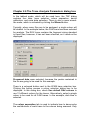
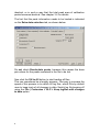
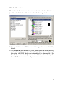
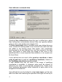
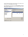
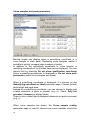
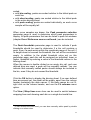
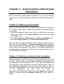
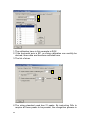
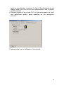
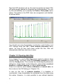
Contents
Chapter 1. Introduction __________________________3
Chapter 1.1. Advantages _______________________________3
Chapter 2. Analysing files containing peak information5
Chapter 2.1. Opening data files __________________________5
Chapter 2.2. The Trace Analysis Parameters dialog box _____6
Chapter 2.3. Colour views ______________________________9
Chapter 2.4. Binning sheets____________________________12
Chapter 2.4.1. Binning sheet menu options_________________________ 18
Chapter 2.5. Defining bins _____________________________18
Chapter 2.6. Exporting the binning sheet _________________20
Chapter 3. Analysing files without peak information_21
Chapter 3.1. Setting up peak analysis____________________21
Chapter 3.2. Setting up sizing standard recognition ________21
Chapter 3.3. Opening data files _________________________24
Chapter 3.4. Normalising data __________________________25
Chapter 3.4.1. Normalising: Equalise peak areas ____________________ 25
Chapter 3.4.2. Normalising: Equalise named peaks __________________ 26
1
Chapter 1. Introduction
DAx can be used to read and analyse trace files such as the files
that are created by the Amersham MegaBACE™ and ABI
Genescan® systems.
Gel scoring involves the alignment of large numbers of
measurement traces, and the localisation of bins of peaks in those
traces. This manual describes how to perform such analyses.
Chapter 1.1.Advantages
Some of the advantages DAx offers for the type of analysis
described in this manual are:
• ability to read all ABI Genescan files (*.fsa), including ABI 3730
files
• ability to read Amersham MegaBACE files
• ability to read SCF files
• ability to read and handle ABI files that have not been called yet
with Genescan, as well as ABI files for which no BP calibration
has been determined yet. BP sizes of standard peaks can be
read from ABI files, with no need to have a separate
standards.cfg file
• fully featured baseline construction / peak find ability
• simultaneous display of colour view (gel view) and binning sheet
containing curve samples
• easy maintenance of user defined bins (including easy deletion)
• fully customisable colours and sizes
• binning sheet export of PHYLIP and PAUP formats; binning
sheet export of tab delimited text files (including full column
labels); binning sheet export of thumbnail views as RTF Word
Processor files
• ability to handle several thousand files simultaneously
• fully supported software: problems are solved generally within 24
hours
3
Chapter 2. Analysing files containing
peak information
Some ABI measurement files contain peak calls in addition to the
data traces. DAx is able to import those peak calls so that they can
be used to set up the binning process.
Use the following procedure to open such files and analyse them.
Chapter 2.1.Opening data files
1. Invoke the File | Open command. Select Files of Type ABI
Genescan®. Select the file or files you want to analyse; you can
select several hundreds of files at once.
2. Do not check the Multiple windows box. There is no need to
check the Automatic analysis box.
3. Optionally, you may check the Colour view box. Doing this
causes the data to be displayed as a colour view (“gel”) image
after they have been loaded.
4. Click the Open button. This will start loading the trace files.
5. The Trace Analysis Parameters dialog box is displayed.
5
Chapter 2.2.The Trace Analysis Parameters dialog box
In the tabbed mode, which will be used here, the TAP dialog
contains four tabs: trace selection, colour separation, derive
calibration, and extra data selection. There is also a more wizardlike mode, which is activated by clicking the Wizard button.
Typically, when many files are to be analysed, a single colour will
be studied. In the example below, the FAM trace has been selected
for analysis. The ROX trace contains the fragment sizing standard
in these files; however, it has not been checked, as it need not be
displayed.
Processed data were selected, because the peaks contained in
the file are going to be used for this example.
There is a coloured button next to the 6FAM trace selection box.
Clicking this button causes a colour selection dialog box to be
displayed. In this dialog box, check Use default DAx colours to
use 12 different colours for the traces. Alternatively, select a single
colour to be used for all FAM traces. In the example, dark blue is
selected.
The colour separation tab is used to indicate how to deconvolve
the contributions of each trace to the colours being scanned. Only
6
raw data needs deconvolution; if processed data are loaded, the
deconvolution has already taken place. Some ABI files contain an
internal deconvolution matrix, which can be used.
The Derive calibration tab is used to set up the way the sizing
standard is derived for the data being loaded. Typically, the Derive
DNA calibration from option will be selected. In the example, the
calibration is contained in the ROX trace.
There are several ways that DAx can derive the calibration from the
ROX trace. In our first example, the ABI files contain peak
information, including base pair sizes, which DAx will use to set up
the sizing calibration 1.
Check the Convert to BP axis option to make DAx convert the
data to a base pair axis after they have been loaded This step is
not required, but can increase processing speed.
Check Normalise data to normalise the data. Configure
normalisation by clicking the Config button. Typically, the data will
be normalised in such a way that total peak areas become
1 The FAM trace also contains sizing information, which was derived by the
Genescan software from the ROX trace’s sizing standard. Checking the FAM
trace as the source of the calibration is therefore possible – but not
recommended.
7
identical, or in such a way that the total peak area of calibration
peaks becomes identical. See chapter 3.4 for details.
The fact that the peak information needs to be loaded is indicated
on the Extra data selection tab, as shown below.
Do not check Recalculate peaks, because this causes the base
pair values for the peaks contained in the file to be lost.
Now click the OK to All button to start loading all files.
This can sometimes be a lengthy process. One way to increase the
speed of this process is to switch off log files, which DAx by default
uses to keep track of all changes to data. Switch log file keeping off
using the File | Customise > GLP > Keep logfiles with changes
to data option.
8
Chapter 2.3.Colour views
Unless the Colour view option was checked in the File | Open
dialog box, the data are now displayed as traces.
Each data trace is represented by a data tag. In this example, 12
files were opened; the data tags are displayed above the graph.
Notice the padlock symbol in 11 of the data tags. This symbol
indicates that peak data were loaded fixated, i.e. with known height,
area, and base pair size from the files. One data tag does not show
a padlock symbol – this file contained no peak data.
9
To display the data as a colour view, use the View | Colour view
menu option.
The view menu of this colour view window contains a number of
important options:
• extra space (used here) causes some white space to be
displayed between lanes 2.
• use trace colours (used here) causes the colours of the FAM
traces to be used to create the gel image. Alternatively, a full
spectrum of colours is used to denote signal strengths,
somewhat like a topographical map. The View | Attributes
option is used to select those colours.
• halftones causes fluent colour transitions to be used between
data points.
• subtract baselines subtracts baseline signal strength from the
data (and hides the baselines from the colour view). In this
example, no baselines are being used.
• separate lanes / group per lane is not relevant here, because
only FAM traces were loaded. If additional traces were loaded, all
2 The “white space” can be any colour. Use the View | Attributes menu option
to select colours for the axes, the area around the area, and the area inside
the axes.
10
traces from a single file could be displayed in a single lane using
the group per lane option. In this example, separate lanes are
displayed.
• calibrated axis causes the colour view to be displayed with a
base pair axis, even if the data have not been converted to a BP
axis. If no calibration is available for a trace, it will not be
displayed. In this example, calibrated axes are necessarily used,
because the data have been converted to a BP axis.
• mark peaks and bins (used here) causes the bins that have
been defined or have been derived to be marked using dotted
lines. If the bins have been user defined, they can be adjusted, or
more can be added. This option also causes peaks present in the
data to be marked with small triangles.
It is possible to zoom in on the image by clicking and dragging the
mouse cursor across the area of interest.
Use the View | Attributes > Spacing > Lane height item to set a
minimum height per lane. By default this is set to 20 pixels. If more
lanes exist than will fit using this minimum lane height, DAx will
automatically display vertical scroll bars.
The example image appears a little washed out, because its
scaling is based on a single very high peak (signal top at 6209 AU).
It is possible to “zoom in on the colour scale”, by clicking and
dragging on the colour bar to the right of the colour view.
11
Zooming in on the colour scale, as well as on the left side of the
colour view, gives something like the image displayed below.
Chapter 2.4.Binning sheets
Binning sheets are used to inspect the similarities and differences
between the peaks found in many data sets. Each line in a binning
sheet pertains to one group of peaks across all data sets; each row
corresponds to a data set 3.
Before defining bins, make sure to remove all pre-existing binning
information using the Analysis | Clear binning sheet menu option.
To set up the binning sheet use the Analysis | Binning sheet
menu option. A dialog box is displayed with a parameter selection
area at the left side. A binning sheet uses over 10 sets of
parameters, which can be easily navigated here, either by using the
Next and Prev buttons, or by clicking on any of the parameter set
names. Not all sets of parameters are discussed below; refer to the
DAx User’s manual for the complete list.
3 An exception occurs when binning lines are wrapped, so that a bin is spread
across multiple lines, rather than a very wide single line.
12
Data Set Selection
The first set of parameters is concerned with selecting the traces
(or data sets) that should be included in the binning sheet.
1
2
1. Trace selection area. All traces containing peaks are selected by
default.
2. The Select all item allows the quick selection of all data sets that
meet certain criteria, across all graphic windows. For instance, all
data sets with ROX labels can be selected (or deselected if the
Deselect box is checked). Press the Alt key when clicking the
Select All button to remove all previous selection.
13
User defined or automatic bins
Checking User defined bins allows the user to define bins, rather
than having bins automatically derived. Bins are typically defined
using a colour view window (see chapter 2.5).
The bins equal peaks option, available when user defined bins are
used, causes all existing peaks to be removed from data sets that
are added to the binning sheet. New peaks, with coordinates
exactly equal to all user defined bins, are then created in the data
sets. This option is used when the shape of the curve in the
predefined bins is more important than whether or not a peak can
be found there.
If user defined bins are used, either peak top coordinate or base
pairs at peak top is used as a qualifying coordinate, chosen on
the Qualifying coordinate parameter page.
If user defined bins are not used, a full range of qualifying
coordinates is available. A tolerance value must be entered to
determine the width of automatically assigned bins. Peaks must
have qualifying parameters within tolerance of each other to be
assigned to the same bin.
User defined bins can be limited to certain trace types, so that only
data from data sets matching the specified trace type will end up in
14
the bin. Each bin can have its own trace type. This option can be
selected on the Trace types parameter page.
User defined bins can be set up on the Bin intervals parameter
page, as shown below. They can also be defined using a colour
view window, cf. chapter 2.5.
15
Curve samples and peak parameters
Binning sheets can display either a quantifying coordinate or a
curve sample of each peak. Displaying curve samples makes it
possible to quickly compare large numbers of peaks.
In addition to the quantifying coordinate or curve sample, a
qualifying coordinate or list of peak data can be displayed. You can
prevent this by checking Do not show qualification coordinate
(when a quantifying parameter is displayed) or Do not show peak
parameters (when curve samples are drawn).
When a quantifying coordinate is displayed, it is chosen on the
Quantifying coordinate or label parameter page. Choices include
peak height and peak area.
Instead of a quantifying coordinate, you can choose to display just
a label whenever a peak is present (e.g. +). Check Only list
presence / absence to display labels.
There is also a label that is displayed whenever no peak is present
(e.g. --).
When curve samples are drawn, the Curve sample scaling
parameter page is used to choose how curve samples should be
16
scaled.
• with bin scaling, peaks are scaled relative to the tallest peak on
each line
• with sheet scaling, peaks are scaled relative to the tallest peak
in the entire binning sheet
• with peak scaling, peaks are scaled individually, so each curve
sample will be equally tall
When curve samples are drawn, the Peak parameter selection
parameter page is used to determine which peak parameters to
display. All peak parameters that can be listed in peak list windows
(chapter Error! Reference source not found.) can be included.
The Peak thresholds parameter page is used to indicate if peak
thresholds should be used to determine if a bin cell contains a
peak. Even if a peak exists within the coordinate range of the cell, if
its height does not exceed the threshold, the cell will be considered
empty. In addition to the global threshold value set on this
parameter page, each bin can be assigned an individual, lower or
higher, threshold by entering a value in the threshold column in the
binning sheet.
When the mouse is double clicked on an empty bin cell, and user
defined bins are used, a peak will be manually added4. You can
indicate that manually added peaks should always be included in
the bin, even if they do not exceed the threshold.
Click the OK button to display the binning sheet. If no user defined
bins are present yet, the sheet will be empty, apart from the column
header containing the data names. If the data names do not fit,
right click on the column header, and use the Fit columns menu
option.
The View | Wrap lines menu item can be used to switch between
wrapping lines and showing each bin on a single horizontal line.
4 If user defined bins are used, you can also manually add a peak by double
clicking on a colour view.
17
Chapter 2.4.1.Binning sheet menu options
The Binning Sheet has the usual text window menu options. Other
than in the usual text export formats, binning sheet contents can be
exported in PAUP and PHYLIP formats using the File | Export
menu option.
When the right mouse button is clicked in the sheet, a popup menu
appears.
The popup menu offers the ability to locate or highlight a peak or
bin in a graphic window (press the Shift key to hide all other data
sets), or to highlight all selected peaks.
If user defined bins are used, the Insert peak and Remove peak
menu options are used to insert a peak in the location of the bin cell
that was clicked on, or remove an existing peak. Double clicking on
the binning cell has the same effect.
The Display single bin menu option limits the binning sheet to
displaying a single bin. You can then use the Previous bin, Next
bin, View | Previous bin, View | Next bin options to navigate to
the previous or next bin. Use All bins or View | All bins to once
again display all bins.
If user defined bins are used, bins can be removed using Remove
bin or Remove selected bins. A new bin can be defined using the
Add bin option.
Chapter 2.5.Defining bins
There are two ways to define a bin using the colour view window.
Make sure the View | Mark binning sheet bins option is active for
the colour view!
1. Press the Ctrl key, and click and drag a rectangle on the colour
view where the bin should be.
2. Double click on a peak marker in the colour view. This will add a
bin starting and ending at the peak’s boundaries. This option will
not work if the View | Group per lane option is in effect, since
there would be multiple peaks present per lane.
18
Bins will be marked in the colour view using dotted lines. To resize
a bin, click and drag the dotted line. To remove a bin, drag its
starting dotted line beyond its ending dotted line, or vice versa.
To display only a single bin in the binning sheet, click the right
mouse button on a bin, and select Display single bin from the
popup menu. Use View | Next bin and View | Previous binto
navigate to different bins. Use View | All bins to display all bins
again.
The display below shows the result after some 6 bins have been
defined. Note the binning sheet, which now contains curve samples
from all bins.
As the mouse is moved over the colour view, the appropriate curve
sample in the binning sheet is brought into view and highlighted. To
stop this behaviour (for instance when the curve sample you
wanted has been highlighted, and you want to move the mouse
cursor over to it), press the Shift key.
Clicking the right mouse button on the binning sheet and choosing
the locate peak menu option zooms the colour view as well as the
trace graph in on the peak.
19
To change the height of the binning sheet lines, place the mouse
cursor in between two lines, until it changes to an up-down arrow.
Then click and drag to set a new line height.
If a bin does not contain a peak, but a peak should be present,
double click either in the binning sheet or in the appropriate location
in the colour view5. Conversely, double clicking when a peak is
present removes it.
Chapter 2.6.Exporting the binning sheet
The binning sheet can be printed using the File | Print command. If
the contents are too wide for a single page, multiple side-by-side
pages can be printed by choosing the tiled option in the print
dialog.
Using the File | Export menu option, the contents of the binning
sheet can be exported in a number of formats:
• As a Nexus file
• As a PHYLIP file
• As a (tabbed) text file
• In Rich Text Format, which can be read into most word
processing software. Even binning sheets containing curve
samples can be exported in this format.
5 Note that double clicking on the colour view has two functionalities: inside a
bin, it adds or removes a peak, outside a bin it adds a bin based on the peak
being clicked on (if any).
6 Unless Windows has been set up to use a different application to open these
types of files.
20
Chapter 3. Analysing files without peak
information
Not all trace files contain peak information, or you may not always
want to use it. In these instances, DAx can be used to find peaks in
data.
Chapter 3.1.Setting up peak analysis
To set up peak analysis, open a single representative file using the
File | Open menu option. Unlike the procedure described before,
you should:
• check the calibration trace (here: ROX), as well as the unknown
trace (here: FAM) on the Trace selection tab of the TAP dialog
(cf. Chapter 2.2).
• check Do not derive calibration on the Derive calibration tab.
• not check Import peaks on the Extra data selection tab.
This will load the FAM and ROX traces, without analysing them.
Now, first use the Peaks | Construct baselines menu option to
construct baselines for the data. Then use the Peaks | Find peaks
menu option to find peaks in the data. For a detailed discussion of
the parameters for baseline construction and peak finding refer to
the DAx Quick Start Guide.
Chapter 3.2.Setting up sizing standard recognition
Sizing standards consist of a number of fragments with known base
pair size. The best way to recognise the standard’s fragments is to
use Automatic Trace Calibration, ATC. To do this, DAx needs to be
told about the sizing standard by entering the base pair counts. A
few additional parameters are used to instruct DAx on how to
determine which peaks are part of the standard, and which are not.
A
full
explanation
of
ATC
can
be
found
at
http://www.dax.nl/daxatc.pdf. Below the ATC parameter dialog box,
which is invoked using the Analysis | Edit ATC menu option, is
shown.
21
1
2
3
1. The calibration trace in this example is ROX.
2. If the horizontal axis is BP, no sizing calibration can usefully be
derived; those data are therefore excluded here.
3. The list of sizes.
4
5
4. The sizing standard used has 21 peaks. By instructing DAx to
require all those peaks to be present, the recognition process is
22
sped up considerably. However, if a few of the standards do not
always show up at the end of the measurement, use a slightly
smaller number
5. Requiring peaks to be at least 0.2% of total area weeds out small
and insignificant peaks, again speeding up the recognition
process.
6
6. Indicate what sort of calibration is to be used.
23
Now that ATC has been set up, the next time peaks are found, DAx
will automatically attempt to recognise the sizing standard. You can
try this immediately, by re-issuing the Peaks | Find peaks menu
option. The peaks in the ROX trace are recognised, and labelled,
as shown below.
You should now save the baseline construction, peak finding, and
ATC settings using the File | Save analysis procedure menu
option. As long as they have been saved like this, DAx will
automatically load them next time it starts.
Chapter 3.3.Opening data files
As in chapter 2.1, use the File| Open menu option to select a large
number of files. This time, check the Automatic analysis box, and
click the Config button. This invokes the AutoAnalysis preferences
dialog box, shown below. In the dialog box, select either construct
baseline or subtract baseline, as well as detect peaks.
There is no need to check derive calibration or convert axis, as
this is done in the TAP dialog (cf. Chapter 2.2).
A note on the use of subtract baseline: if a baseline is
constructed, it may immediately be subtracted from the data using
this option. However, it is also possible to use subtract baseline
24
without first constructing a baseline. In this case, the data will be
marked as having a baseline subtracted. This option should only be
used with data that already have a zero baseline; its use is not
recommended.
When the automatic analysis options have been selected, click the
OK button to leave the dialog box. Then click the Open button to
start loading files.
The TAP dialog will be displayed. Fill it in just as in chapter 2.2, but
do not check the Import peaks box on the Extra data selection
tab7. Click the OK to All button to load all selected data files. Now,
proceed as in chapter 2.3.
Chapter 3.4.Normalising data
On the Derive calibration tab in the TAP dialog box, you may
check the Normalise data box to force data to be normalised after
they have been loaded. Click the Config button to set up
normalisation.
Typically, no horizontal normalisation will be employed. There are
two main vertical normalisations.
Chapter 3.4.1.Normalising: Equalise peak areas
Equalising peak areas takes three parameters:
• percentage smallest peaks to use, this can be 100% to
consider all peaks
• target total peak area, typically, you should use a value that
does not change the sizing of the data too much; it may be better
to use the following option
• derive from first data set encountered, this option uses the
total peak area of the first data set loaded as the target total area
for all data sets
7 In fact, the peaks would be superseded.
25
Chapter 3.4.2.Normalising: Equalise named peaks
Equalising peak areas takes three parameters:
• in trace, this defines the trace in which to look for named peaks;
this is almost always the trace that contains the sizing standard.
Using the total area of the sizing standard peaks as the basis for
normalisation makes sense because typically the amount of
sizing standard will be equal through all measurements
• target total named peak area, typically, you should use a value
that does not change the sizing of the data too much; it may be
better to use the following option
• derive from first data set encountered, this option uses the
total named peak area of the first data set loaded as the target
total area for all data sets
Note that when named peaks are used as the basis for
normalisation, all traces from a single file will be sized identically,
all based on the selected in trace.
26