Download Automatic Trace Calibration (ATC)

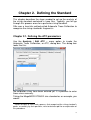
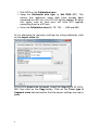
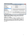
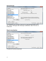
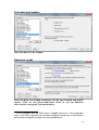
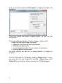
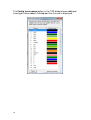
Contents
Chapter 1. Introduction _________________________ 3
Chapter 2. Defining the Standard _________________ 5
Chapter 2.1. Defining the ATC parameters ________________ 5
Chapter 2.2. Troubleshooting ATC _____________________ 10
Chapter 3. Analysis of the Calibration Ladder _____ 11
Chapter 3.1. Trace Analysis Parameters (TAP) dialog______ 12
Chapter 3.2. Results _________________________________ 21
Chapter 4. Analysis of the Unknowns ____________ 24
Chapter 4.1. Trace Analysis Parameters (TAP) dialog______ 25
Chapter 4.2. Results _________________________________ 29
Chapter 4.3. Converting to a Base Pair axis ______________ 30
Chapter 4.4. Normalising the data ______________________ 31
Chapter 4.5. Displaying data as a colour view ____________ 32
Chapter 5. Trace Types in DAx __________________ 33
Chapter 5.1. Assigning trace types _____________________ 33
Chapter 6. Conclusion _________________________ 35
1
Chapter 1. Introduction
DAx can be used to read and analyse trace files such as the files
that are created by the Amersham MegaBACE™ and ABI
Genescan® systems.
The MegaBACE™ and ABI systems, like other DNA analysis
systems, can analyse four or five traces in a single run, using four
(five) different (coloured) labels. One way to use this feature is to
include a standard sample with known DNA fragment sizes as one
of the traces, and apply this standard to the other traces. The
standard is used to ascertain the fragment sizes of the components
in the unknown samples.
3
Chapter 2. Defining the Standard
This chapter describes the steps needed to set up the analysis of
the sizing standard contained in trace files. Typically, you will go
through this process once for a particular sizing standard.
DAx uses a heuristic method called Automatic Trace Calibration to
recognise the sizing standard’s fragments1.
Chapter 2.1. Defining the ATC parameters
Use the Analysis | Edit ATC .. menu option to invoke the
Automatic Trace Calibration, or ATC, dialog box. The dialog box
looks like this:
No calibration sizes have been entered yet. It is possible to enter
these sizes manually.
Taking the MegaBACE ET550-R size standard as an example, you
would:
1 Earlier versions of DAx used a process that recognised the sizing standard’s
peaks, essentially, by their positions; refer to daxtrace.pdf for an explanation of
this procedure.
5
• Pick ROX as the Calibration trace
• Keep the Horizontal axis type as Not DNA (BP). This
means that whenever some data have already been
converted to a BP axis, the ATC will not be applied. All other
axis types, such as time axes, will have ATC applied,
converting them to a BP axis.
• Enter the Calibration sizes 60, 75, 100, …, 525 and 550
As an alternative to manually entering the sizing calibration, click
on the Import sizes tab.
In the list of predefined standards, select the MegaBACE ET-ROX550, then click on the Copy button. Click on the Trace type &
fragment sizes tab and confirm that the correct settings are now in
place.
6
In order to set up some restrictions, click on the Restrictions tab.
These restrictions, while ideally not required, can significantly
speed up the ATC process.
Here, Require minimum number of calibration points has been
made active, and the total number of sizes in the ET550-R
standard, 22, has been entered. Note that if some measurements
have been run short, they may not contain all 22 standard sizes. In
this case, the minimum number of sizes will have to be lowered.
Require minimum peak area has also been made active, with a
minimum peak area of 0.2%. This filters out any really small peaks
from consideration as a sizing standard peak.
A similar effect could be achieved by limiting ATC to a number of
the largest peaks expressed in the ROX trace. If n standard peaks
are present, a value of 2n generally works well.
Some measurements will have very tall peaks early in the
measurement, which may bleed through into the ROX trace. When
that happens, it can be helpful to exclude an initial time range2.
2 Under these circumstances it is sometimes also necessary to leave out two
or three of the initial sizes in the standard from the list of sizes, because those
low sizes (60, 75) would have been expressed in the initial time range.
7
Click on the Calibration tab to indicate the type of calibration that
should be set up.
8
Click on the Advanced tab to set up some advanced option.
Start looking for highest size runs the ATC algorithm “in
reverse”, which can sometimes be helpful.
Allow missing points at both start and end allows for low end as
well as high end calibration points to be missing.
Reward higher numbers of calibration points tells the ATC
algorithm that searches that turn up more calibration points are to
be considered better.
Reward higher total calibration peak area percentage tells the
ATC algorithm that calibration points are likely to have peaks with
significant sizes.
Reward calibration peak areas being similar instructs the ATC
algorithm to make use of the fact that calibration peaks probably
have similar sizes.
Maximum allowed discontinuities can be used if the
measurement is known to contain a discontinuity in the horizontal
axis. It is rarely necessary to allow discontinuities.
The low and high allowed direction ratios determine how
forgiving the ATC algorithm will be. More forgiving settings (further
away from 1.0) will result in more inclusive searches, which may
take longer to run. Generally, values of 0.7 and 1.5 give excellent
results.
9
Once all fields have been filled, click the Close button to close the
ATC dialog. You should now use File | Save Analysis Procedure
to store this setup on disk.
Chapter 2.2.Troubleshooting ATC
In the next chapter, Automatic Trace Calibrations will be used to find the
standard peaks in a ROX trace. This is normally a very straightforward
process. However, should the procedure run into a snag, there are some steps
that should be followed.
The first step is to make sure that the calibration trace being looked at does
indeed contain all (or some) expected calibration peaks. Here are some
reasons why this might not be the case:
• the most common reason is that too large an interval at the start of the trace
is being excluded from peak finding, causing one or more initial calibration
peaks to be skipped. Make sure not to skip too large an interval at the start
of the trace when finding peaks.
• peak find parameters might have too high a detection limit.
• the trace may actually not contain the calibration peaks, or not all of them. If
10 calibration peaks are expected, but only 8 peaks are present, ATC will
fail if the require minimum number of calibration points parameter was
set higher than 8.
If the calibration peaks are present and found correctly, but ATC still fails,
some parameters may have been given values that are too limiting. It is
important to understand that most ATC parameters are used to speed up the
ATC algorithm, without being strictly necessary for the algorithm to work.
Therefore, if the ATC fails to find a calibration, these parameters can be
relaxed, advisably in this order:
• if some early sizes are being missed, skip a smaller interval
• if you are sure all sizes are present, and early sizes sometimes get called
wrong, use the advanced option Start looking for highest size
• require a smaller peak area
• use more peaks
• require fewer points to be present
10
Chapter 3. Analysis of the Calibration
Ladder
Invoke the File | Open command. Select Files of Type ABI
Genescan files (or one of the other trace file types: SCF files,
MegaBACE files CEQ files), select a file containing the calibration,
then click the Open button.
The options at the bottom of the File | Open dialog are discussed in
the next chapter.
Note that typically each sample file will contain the calibration
ladder, so any sample file can be selected to set up the calibration.
Here, one file contains only the calibration, so this file is used.
11
Chapter 3.1.Trace Analysis Parameters (TAP) dialog
When trace files are opened, the Trace Analysis Parameters (TAP)
dialog is displayed, so that the way in which the data are to be
loaded can be set up. The TAP dialog contains a list of parameters
at left, which you should fill out in order34.
Raw or processed data
The example file contains no processed data, so raw data must be
loaded.
Click Next to display the next page of parameters.
3 The list changes in accordance with the types of parameters that are
needed.
4 If your TAP dialog does not look like the examples, you should click the
Wizard button third from bottom left.
12
Trace names
Some trace files contain the names of the traces used, but the
example does not, instead just specifying Dye1 – Dye4. These
should be changed to recognized dye names, as shown.
The Config trace names button lets you specify new trace names,
and lets you specify standard colours for existing and newly
defined trace names5.
5 A trace name can also be derived from data file names, which is beyond the
scope of this document
13
Trace selection
Choose which traces to load. In this example, we are only
interested in the size calibration ladder, which is measured in the
ROX trace, so only ROX is checked.
Trace drawing colours
The Use standard colours button is disabled here because the
colours are already the standards for the trace names shown.
14
Colour separation method
The signals measured for each of the traces are made up of
contributions of not just the trace itself, but also contain
bleedthrough from the other traces. To correct for that, a colour
separation should ideally be used. The best way to do this is to
specify a colour separation matrix that has been ascertained by
measuring a standard mixture of samples.
Colour separation matrix
15
Sizing calibration derivation
In the example, we want to derive the sizing calibration from the
ROX trace. Note that the list of parameters at left has changed
because the selection on this page was changed from Do not
derive calibration to Derive size calibration from a trace.
The warning symbol displayed next to Compare analysis settings
is there because DAx has detected an inconsistency. This will be
resolved momentarily.
16
Calibration trace selection
By changing the calibration trace to ROX, the warning icon next to
Compare analysis settings is removed. Make sure Use ATC is
checked, so that the ET 550-R calibration that was set up in
Chapter 2 will be applied.
Sometimes it is desirable to analyse the calibration trace with
different baseline construction and peak find parameters than the
other traces. To do that, check Private baseline settings and
Private peak find settings. When these options are checked, the
texts become blue and underlined and can be clicked to set up
parameters.
17
Horizontal axis
The horizontal axis can be a time axis, or can be converted to a BP
axis. When setting up and verifying a calibration, leave the axis as
a time axis.
Signal normalisation
The data will not be normalized.
18
Extra data and headers
No extra data will be loaded
Baselines, peaks
After the data are loaded, baselines will be constructed and peaks
found. Click on the blue-underlined items to set up baseline
construction and peak find parameters6.
6 In this example, only the ROX trace is loaded. Since this is the calibration
trace, it will have a baseline constructed and peaks found even if the baseline
construction and peak find items are not checked here.
19
Maxed-out signal correction
Sometimes the signal values in a trace file will exceed what the
data format can handle. DAx can detect such occurrences and
annotate them in the loaded data.
Compare analysis settings
DAx will compare and verify a number of analysis settings, and flag
any that do not match. In such instances, clicking the Adjust
button will remove the conflict.
20
To finish filling out the TAP dialog, click the Finish button.
Chapter 3.2.Results
The ROX trace will now be loaded and analysed. The result is
shown below.
Note that the calibration peaks are lalebelled with their fragment
sizes. This is because ATC has named each calibration peak with
its fragment size, and peaks are being labelled with their names.
21
To verify that the calibration is well formed, click on the data tag of
the ROX trace, and select the Calibration | Curve menu item from
the popup menu that appears.
For a quick verification of multiple calibrations, try the following:
• Use the File | Open command to once again display the File |
Open dialog. Select multiple data files. Check the Stacked
checkbox at the bottom of the dialog. Click Open.
• In the TAP dialog, click Finish All without changing any
settings.
22
The result might look like this:
Despite running at different times, all 5 calibrations are well
recognised.
23
Chapter 4. Analysis of the Unknowns
Invoke the File | Open command. Select Files of Type ABI
Genescan files (or one of the other trace file types: SCF files,
MegaBACE files CEQ files), Select the file or files you want to
analyse, then click the Open button.
Check Multiple windows if you want each file to be put in its own
window (not typically used for trace analysis).
If you are opening hundreds or thousands of files, you can check
MInimised. The window into which the files are loaded will be
created minimized, so that the traces are not drawn, saving time.
Check Sorted and use the Config button to indicate how the data
will be sorted after loading. For instance, the data can be sorted by
well or plate name.
Opening files as a Colour view creates a gel type view of the data
immediately upon loading.
You can immediately display the data Stacked, and use its Config
button to indicate how to stack.
Automatic analysis is used to create baselines and find peaks
immediately upon loading. For trace files, using the TAP dialog
(see below) is the preferred method, so do not check this option.
Click the Open button to start opening all selected sample files.
24
Chapter 4.1.Trace Analysis Parameters (TAP) dialog
As was mentioned in the previous chapter, when trace files are
opened, the Trace Analysis Parameters (TAP) dialog is displayed,
so that the way in which the data are to be loaded can be set up.
Since we are now analyzing the data, some changes will be made.
Trace selection
The example files only contain data in the FAM trace, so only FAM
and ROX are checked7.
7 It is even possible to check only FAM! The ROX trace will temporarily be
loaded to set up the calibration, and will then be discarded.
25
Horizontal axis
This time, the horizontal axis will immediately be converted to a BP
axis.
Baselines, peaks
For both the ROX and FAM traces, a baseline will be constructed
and peaks will be found.
Let’s look at the baseline construction and peak find parameters.
26
Click on the blue underlined Construct baseline to display the
baseline construction parameters dialog.
The baseline type has been changed to Moving Median, but
elsewhere all settings have been left at factory defaults.
When items are checked to use Auto values, DAx analyses the
data to find values that fit the data being analysed.
27
Click on the blue underlined Find peaks to display the peak find
dialog box.
Trace files should not contain negative peaks, so they are not
being found.
The peak find dialog contains a further 7 pages, dealing with:
• peak find signal and slope thresholds
• skipping an initial part of the measurement
• detecting shoulder peaks
• normalising peak widths to a set number of base pairs
• removing bleed-through peaks
All these settings can be left at factory defaults in almost all
analyses.
To finish filling out the TAP dialog, click the Finish button. If more
than one data file was selected in the File | Open dialog, click
Finish All to load all data without showing the TAP dialog again.
28
Chapter 4.2.Results
The FAM and ROX traces will now be loaded and analysed. The
results might look like this.
The following has happened in succession.
• For each file, the ROX trace is loaded. It was analysed using the
current settings. Since the Automatic Trace Calibration
parameters define ROX as the calibration trace, the sizing
standard was recognised, and a calibration relating time
coordinates to fragment sizes was derived from the ROX trace.
• the FAM traces were loaded and analysed using the current
settings.
• The axis was converted to base pairs using the calibration
derived from the ROX trace.
You can now click any of the peak list buttons at the left side of the
data tags for the ROX or FAM traces. You will note that the correct
fragment sizes are listed in the Base Pairs column.
It is also possible to display the fragment sizes of the peaks that
were found in the graphics window. To do this, invoke the File |
Customise menu option. Select the Plotting Peaks tab. Under
Peak Labeling, select Component Name as the first peak label.
29
Select Base Pairs as the second peak label (it is near the bottom
of the list of possible peak labels). Click the OK button.
The graphic window will now display base pair counts for all the
peaks. You can click and drag the mouse on the graph to zoom in
on the peaks, and see more detail.
Chapter 4.3. Converting to a Base Pair axis
In the example above, the horizontal axis was immediately
converted to a BP axis, by checking Convert to BP axis in the TAP
dialog.
If this option had not been checked, the axis can still be converted
using the Calibration | Axis Conversion menu option. This
displays a dialog box.
Make sure to check the New Window check box, and then make
sure that all data are selected. Note that the dialog box was resized
to make all data items visible by dragging its bottom right corner.
30
Chapter 4.4. Normalising the data
When loading trace data, it can be desirable to normalise the data
after they have been loaded. One common form of normalisation
stretches the data vertically in such a way that the total area of the
size calibration peaks is equal across several measurements.
Normalisation can be achieved after data have been loaded using
the Data | Overlay menu option. A more convenient way to
normalise is to check the Normalise data check box on the Signal
normalization page in the Trace Analysis Parameters dialog box.
Click the Config button to set up normalisation.
In this example, the horizontal axis is not affected.
The vertical axis will be stretched in such a way that the total area
of all named peaks in the ROX trace will become 10000. Named
peaks are used because the named peaks in the ROX trace will be
the calibration standard (as called by ATC).
The other trace (FAM) will be stretched an equal amount as the
ROX data.
31
Chapter 4.5.Displaying data as a colour view
Use the View | Colour view menu option to display the data as a
colour (gel) view.
As always, you can zoom in on the colour view by clicking and
dragging the mouse.
The colour view window’s View menu has a number of options that
govern how things are displayed. In the example above, there is
extra space between lanes, each trace is displayed using its own
trace colour, colours are displayed darker to make them easier to
read, the baseline has been subtracted, each trace is in a
separate lane (as opposed to have all traces from a file displayed
in a single lane), a calibrated axis (BP) is used, and peaks are
marked.
32
Chapter 5. Trace Types in DAx
Trace types are used in DAx for a number of purposes.
Their principal use is to distinguish between up to five traces that
can be contained in a single measurement file, where obviously the
file name alone would be insufficient.
A secondary use is to limit certain operations to specific trace
types. These operations include:
• Automatic Trace Calibrations. The trace type is used to indicate
which trace contains the sizing calibration, cf Chapter 2.1.
• Normalise using the total peak area of named peaks of a
specified trace type, cf. Chapter 4.4.
• Identification Database and Marker Peak items. The trace type is
used to limit the detection of certain components to a specified
trace type.
Chapter 5.1.Assigning trace types
DAx attempts to retrieve the trace type of each trace from the
measurement file, which often (but not always) contains trace
names. The trace names are displayed in the TAP dialog, cf.
Chapter 3.1.
The standard trace types that DAx recognises are FAM, HEX, JOE,
NED, ROX, TAMRA, TET, VIC, PAT, LIZ, GRODY, and PET.
Mainly for use with SCF files, there are also A, C, G and T trace
types.
33
The Config trace names button in the TAP dialog allows additional
trace types to be added. A dialog box like this one is displayed:
34
Chapter 6. Conclusion
DAx can be used to perform highly complex analyses of trace files
with relatively little effort.
There are a large number of additional features that have not been
discussed in this manual. Examples are:
• peak width standardisation. If a sample is known to contain
mostly peaks that have a width of 1 fragment, DAx can be told to
preferentially assign peak widths of 1 fragment. If a peak is
clearly wider, its width will not be affected.
• command line analyses. Typically, trace analysers will be used
to perform dozens to hundreds of analyses per day. To make it
possible to analyse such large quantities of data, DAx can be
run from batch files. All the data on an entire hard disk can be
analysed with a single command, while highly flexible report files
are created.
These features exceed the scope of this manual. Refer to the DAx
User’s Manual for details.
35