1
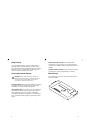
User Manual
TDS3AAM
Advanced Analysis
Application Module
071-0946-00
*P071094600*
071094600
Copyright © Tektronix, Inc. All rights reserved.
Tektronix products are covered by U.S. and foreign patents,
issued and pending. Information in this publication supercedes
that in all previously published material. Specifications and
price change privileges reserved.
Tektronix, Inc., P.O. Box 500, Beaverton, OR 97077
TEKTRONIX, TEK, TEKPROBE, and Tek Secure are
registered trademarks of Tektronix, Inc.
DPX, WaveAlert, and e*Scope are trademarks of
Tektronix, Inc.
WARRANTY SUMMARY
Tektronix warrants that the products that it manufactures and
sells will be free from defects in materials and workmanship
for a period of one (1) year from the date of shipment from an
authorized Tektronix distributor. If a product proves defective
within the respective period, Tektronix will provide repair or
replacement as described in the complete warranty statement.
To arrange for service or obtain a copy of the complete
warranty statement, please contact your nearest Tektronix sales
and service office.
EXCEPT AS PROVIDED IN THIS SUMMARY OR THE
APPLICABLE WARRANTY STATEMENT, TEKTRONIX
MAKES NO WARRANTY OF ANY KIND, EXPRESS OR
IMPLIED, INCLUDING WITHOUT LIMITATION THE
IMPLIED WARRANTIES OF MERCHANTABILITY AND
FITNESS FOR A PARTICULAR PURPOSE. IN NO EVENT
SHALL TEKTRONIX BE LIABLE FOR INDIRECT,
SPECIAL OR CONSEQUENTIAL DAMAGES.
Contacting Tektronix
Phone
1-800-833-9200*
Address
Tektronix, Inc.
Department or name (if known)
14200 SW Karl Braun Drive
P.O. Box 500 Beaverton, OR 97077 USA
Web site
www.tektronix.com
Sales support
1-800-833-9200, select option 1*
Service support
1-800-833-9200, select option 2*
Technical
support
Email: [email protected]
Contents
Safety Summary . . . . . . . . . . . . . . . . . . . . . . . . . . . .
TDS3AAM Overview . . . . . . . . . . . . . . . . . . . . . . . . .
Installing the TDS3AAM Application Module . . . . . . .
Accessing Advanced Analysis Menus . . . . . . . . . . . .
Measurement Functions . . . . . . . . . . . . . . . . . . . . . .
FFT Math Functions . . . . . . . . . . . . . . . . . . . . . . . . .
DPO Math Functions . . . . . . . . . . . . . . . . . . . . . . . . .
Advanced Math Functions . . . . . . . . . . . . . . . . . . . . .
XY Cursors . . . . . . . . . . . . . . . . . . . . . . . . . . . . . . . .
Appendix A: FFT Concepts . . . . . . . . . . . . . . . . . . . .
2
5
6
6
8
12
22
24
31
40
1-800-833-9200, select option 3*
1-503-627-2400
6:00 a.m. – 5:00 p.m. Pacific time
*
This phone number is toll free in North America. After
office hours, please leave a voice mail message.
Outside North America, contact a Tektronix sales office
or distributor; see the Tektronix web site for a list of
offices.
1
Safety Summary
To avoid potential hazards, use this product only as
specified. While using this product, you may need to
access other parts of the system. Read the General Safety
Summary in other system manuals for warnings and
cautions related to operating the system.
Preventing Electrostatic Damage
CAUTION. Electrostatic discharge (ESD) can
damage components in the oscilloscope and its
accessories. To prevent ESD, observe these
precautions when directed to do so.
Handle Components Carefully. Do not slide sensitive
components over any surface. Do not touch exposed
connector pins. Handle sensitive components as little as
possible.
Transport and Store Carefully. Transport and store sensitive
components in a static-protected bag or container.
Manual Storage
The oscilloscope front cover has a convenient place to
store this manual.
Use a Ground Strap. Wear a grounded antistatic wrist strap
to discharge the static voltage from your body while
installing or removing sensitive components.
Use a Safe Work Area. Do not use any devices capable of
generating or holding a static charge in the work area
where you install or remove sensitive components.
Avoid handling sensitive components in areas that have a
floor or benchtop surface capable of generating a static
charge.
2
3
TDS3AAM Overview
This section provides an overview of the TDS3AAM
Advanced Analysis application module features and
describes how to access the advanced analysis functions.
You can do the following analysis tasks with the
TDS3AAM application module:
H DPO Math.
H Arbitrary math expressions. Allow you to create
waveforms using math operations on active and
reference waveforms, waveform measurements, up to
2 user-definable variables, and arithmetic expressions.
H Fast Fourier Transform (FFT) waveform analysis.
H Waveform area and cycle area measurements.
H Measurement statistics. Adds min/max or
mean/standard deviation readouts to displayed
measurements.
H XY waveform cursors.
4
5
Installing the TDS3AAM Application Module
Refer to the TDS3000 & TDS3000B Series Application
Module Installation Instructions for instructions on
installing and testing your TDS3AAM Advanced Analysis application module.
Accessing Advanced Analysis Menus
The TDS3AAM Advanced Analysis module adds Area,
Cycle Area, and statistical measurement functions to the
Measure menu, and FFT, DPO math, and Advanced
Math functions to the Math menu, and XY cursors to the
Cursor menu. To access the Advanced Analysis functions, use the following table:
Accessing TDS3AAM Functions
Function
Push
front
panel
button
Push
bottom
menu
button
Area,
Cycle Area
measurement
MEASURE Select
Measrmnt
Measurement
Statistics
MEASURE Statistics
6
Push side menu
button
–More– button until
you display Area and
Cycle Area buttons.
See page 8.
To select Min/Max or
Mean/Standard Deviation. See page 9.
Accessing TDS3AAM Functions (cont.)
Function
Push
front
panel
button
Push
bottom
menu
button
FFT
MATH
FFT
DPO Math
MATH
DPO Math
Math
waveform
expressions
MATH
Advanced
Math
XY Cursors
CURSOR
Function
Push side menu
button
To select waveform
source, vertical scale,
and FFT window. See
page 12.
To select waveform
sources and operator.
See page 22.
To create a math expression, define a
variable value, define
units, and display the
math expression. See
page 24.
To select Waveform
XY cursor (you must
be in XY display mode
to see this menu). See
page 31.
7
Measurement Functions
The TDS3AAM application module adds Area and
Cycle Area measurements to the Select Measurement
side menu list, and adds a Statistics bottom button to the
Measurement menu. To access these measurement menu
items, push the MEASURE front-panel button.
Area and Cycle Area Measurements (cont.)
Bottom
Side
Description
Statistics
OFF
Disables displaying statistical
information with active measurements.
Min/Max
Displays minimum and maximum
readouts for each active measurement readout.
Mean/
Standard
Deviation
n
Displays Mean and Standard
Deviation readouts for each active
measurement readout.
Area and Cycle Area Measurements
Bottom
Side
Description
Select
Measurmnt
Area
Voltage over time measurement.
The arithmetic area over the entire
waveform or gated region, measured in vertical unit-seconds (for
example, volt-seconds or amp-seconds).
Cycle Area
8
Voltage over time measurement.
The arithmetic area over the first
cycle in the waveform, or the first
cycle in the gated region, measured in vertical-unit-seconds (for
example, volt-seconds or amp-seconds).
n is the number of measurement
values used to calculate the mean
and standard deviation values, and
ranges from 2 to 1000. Use the
general purpose knob to change
the value in increments of 1 (fine)
or 10 (coarse). The default value is
32.
Waveform Polarity. For area calculation, the waveform
area above ground is positive; the waveform area below
ground is negative.
9
Waveform Clipping. For best results, make sure that all
input waveforms do not extend beyond the top or
bottom graticules of the display (referred to as clipping
the waveform). Using clipped waveforms with measurement or math functions can result in incorrect values.
Area. The following equation shows the algorithm for
calculating the waveform area for the entire record or
gated region.
If Start = End then return the (interpolated) value at
Start. Otherwise,
Area=
ŕ
End
Waveform(t)dt
Start
Cycle Area. The following equation shows the algorithm
for calculating the waveform area for a single cycle in
the record or gated region.
If StartCycle = EndCycle then return the (interpolated)
value at StartCycle. Otherwise,
CycleArea=
ŕ
EndCycle
StartCycle
10
Waveform(t)dt
Min/Max. Min/Max displays a minimum and maximum
measurement readout directly below each active measurement. The following is an example of a Min/Max
readout.
Ch1 Freq
15.98 MHz
Min: 15.81MHz
Max: 16.17MHz
Mean/Standard Deviation. Mean/Standard Deviation
displays a mean (m) and standard deviation (s) readout
directly below each active measurement. The mean and
standard deviation values are running calculations,
which means that the current calculation incorporates the
results of previous calculations. The following is an
example of a Mean/Standard Deviation readout.
Ch1 Freq
15.98 MHz
m: 15.99MHz
s: 82.92kHz
Screen Readouts. The Min/Max and Mean/Standard
Deviation readouts display directly below the waveform
measurements, in an area normally used for measurement qualifier text (such as “Low resolution”). If you
suspect the measurement, turn off statistics to see if the
oscilloscope displays any qualifier text.
11
FFT Math Functions
The TDS3AAM application module adds FFT (Fast
Fourier Transform) measurement capabilities to the
oscilloscope. The FFT process mathematically converts
the oscilloscope time-domain signal (repetitive or
single-shot acquisition) into its frequency components,
providing spectrum analysis capabilities.
Being able to quickly look at a signal’s frequency
components and spectrum shape is a powerful research
and analysis tool. FFT is an excellent troubleshooting aid
for:
H Testing impulse response of filters and systems
H Measuring harmonic content and distortion in
systems
H Identifying and locating noise and interference
sources
H Analyzing vibration
H Analyzing harmonics in 50 and 60 Hz power lines
The application module adds the FFT functions to the
Math menu. To access the FFT math menu items, push
the MATH front panel button, and then push the FFT
bottom button.
12
Math FFT menu
Bottom
Side
Description
FFT
Set FFT
Source to
Sets the FFT signal source.
Valid input sources are Ch 1
and Ch 2 (2-channel instruments), Ch 1 through Ch 4
(4-channel instruments), and
Ref 1 through Ref 4 (all instruments).
Set FFT Vert
Scale to
Sets the display vertical scale
units. Available scales are
dBV RMS and Linear RMS.
Sets which window function
(Hanning, Hamming, BlackmanHarris, or Rectangular) to apply
to the source signal. Refer to
page 40 for more FFT window
information.
Set FFT
Window to
Advanced FFT. You can perform FFT analysis on arbitrary
math expressions. See Advanced Math Functions on
page 24 for more information.
Linear RMS Scales. A Linear scale is useful when the
frequency component magnitudes are all close in value,
letting you display and directly compare components
with similar magnitude values.
13
dB Scales. A dB scale is useful when the frequency
component magnitudes cover a wide dynamic range,
letting you show both lesser- and greater- magnitude
frequency components on the same display. The dBV
scale displays component magnitudes using a log scale,
expressed in dB relative to 1 VRMS, where 0 dB =1
VRMS, or in source waveform units (such as amps for
current measurements).
FFT Analysis on Active or Stored Waveforms. You can
display an FFT waveform on any active signal (periodic
or one-shot), the last acquired signal, or any signal stored
in reference memory.
FFT Windows. Four FFT windows (Rectangular, Ham-
ming, Hanning, and Blackman-Harris) let you match the
optimum window to the signal you are analyzing. The
Rectangular window is best for nonperiodic events such
as transients, pulses, and one-shot acquisitions. The
Hamming, Hanning, and Blackman-Harris windows are
better for periodic signals. Refer to page 43 for more
information on FFT windows.
Positioning the FFT Waveform. Use the Vertical POSITION and SCALE knobs to vertically move and rescale
the FFT waveform.
FFT and Acquisition Modes. Waveforms acquired in
Normal acquisition mode have a lower noise floor and
better frequency resolution than waveforms acquired in
Fast Trigger mode due to the higher number of waveform samples.
Do not use Peak Detect and Envelope modes with FFT.
Peak Detect and Envelope modes can add significant
distortion to the FFT results.
Waveforms with DC. Waveforms that have a DC compo-
nent or offset can cause incorrect FFT waveform component magnitude values. To minimize the DC component,
choose AC Coupling on the waveform.
Reducing Random Noise. To reduce random noise and
aliased components in repetitive waveforms, set acquisition mode to average 16 (or more) acquisitions. However,
do not use acquisition averaging if you need to resolve
frequencies that are not synchronized with the trigger rate.
Measuring Transients. For transient (impulse, one-shot)
waveforms, use the oscilloscope trigger controls to
center the waveform pulse information on the screen.
14
15
Zooming an FFT Display. Use the Zoom button
,
along with horizontal POSITION and SCALE controls,
to magnify and position FFT waveforms. When you
change the zoom factor, the FFT waveform is horizontally magnified about the center vertical graticule, and
vertically magnified about the math waveform marker.
Zooming does not affect the actual time base or trigger
position settings.
NOTE. FFT waveforms are calculated using the
entire source waveform record. Zooming in on a
region of either the source or FFT waveform
provides more display resolution but will not
recalculate the FFT waveform for that region.
Measuring FFT Waveforms Using Cursors. You can use
cursors to take two measurements on FFT waveforms:
magnitude (in dB or signal source units) and frequency
(in Hz). dB magnitude is referenced to 0 dB, where 0 dB
equals 1 VRMS. Use horizontal cursors (H Bars) to
measure magnitude and vertical cursors (V Bars) to
measure frequency.
Displaying an FFT Waveform
Do these steps to display an FFT waveform:
1. Set the source signal Vertical SCALE so that the
signal peaks do not go off screen. Off-screen signal
peaks can result in FFT waveform errors.
2. Set the Horizontal SCALE control to show at least
five waveform cycles. Showing more cycles means
the FFT waveform can show more frequency
components, provide better frequency resolution, and
reduce aliasing (page 45).
If the signal is a single-shot (transient) signal, make
sure that the entire signal (transient event and ringing
or noise) is displayed and centered on the screen.
3. Push the Vertical MATH button to show the math
4.
5.
6.
7.
16
menu. If you are in the oscilloscope QuickMenu,
push the MENU OFF button, then push the MATH
button.
Push the FFT screen button to show the FFT side
menu.
Select the signal source. You can display an FFT on
any channel or stored reference waveform.
Select the appropriate vertical scale (page 13) and
FFT window (page 43).
Use zoom controls to magnify and the cursors to
measure the FFT waveform (page 16).
17
FFT Example 1
T
A pure sine wave can be input into an amplifier to
measure distortion; any amplifier distortion will
introduce harmonics in the amplifier output. Viewing the
FFT of the output can determine if low-level distortion is
present.
You are using a 20 MHz signal as the amplifier test
signal. You would set the oscilloscope and FFT parameters as listed in the table:
1
1
2
FFT Example 1 Settings
3
Control
Setting
CH 1 Coupling
AC
Acquisition Mode
Average 16
Horizontal Resolution
Normal (10k points)
Horizontal SCALE
100 ns
FFT Source
Ch 1
FFT Vert Scale
dBV
FFT Window
Blackman-Harris
18
M
The first component at 20 MHz (figure label 1) is the
source signal fundamental frequency. The FFT waveform also shows a second-order harmonic at 40 MHz (2)
and a fourth-order harmonic at 80 MHz (3). The presence of components 2 and 3 indicate that the system is
distorting the signal. The even harmonics suggest a
possible difference in signal gain on half of the signal
cycle.
19
FFT Example 2
T
Noise in mixed digital/analog circuits can be easily
observed with an oscilloscope. However, identifying the
sources of the observed noise can be difficult.
The FFT waveform displays the frequency content of the
noise; you may then be able to associate those frequencies with known system frequencies, such as system
clocks, oscillators, read/write strobes, display signals, or
switching power supplies.
The highest frequency on the example system is
40 MHz. To analyze the example signal you would set
the oscilloscope and FFT parameters as listed in the
following table:
1
2
M
FFT Example 2 Settings
Control
Setting
CH 1 Coupling
AC
Acquisition Mode
Sample
Horizontal Resolution
Normal (10k points)
Horizontal SCALE
4.00 ms
Bandwidth
150 MHz
FFT Source
Ch 1
FFT Vert Scale
dBV
FFT Window
Hanning
20
1
Note the component at 31 MHz (figure label 1); this
coincides with a 31 MHz memory strobe signal in the
example system. There is also a frequency component at
62 MHz (figure label 2), which is the second harmonic
of the strobe signal.
21
DPO Math Functions
The TDS3AAM application module adds the ability to
perform dual waveform math on DPO waveforms. The
resulting DPO math waveform contains intensity or gray
scale information that, like an analog oscilloscope,
increases waveform intensity where the signal trace
occurs most often. This gives you more information
about signal behavior. To access the DPO math menu,
push the MATH front-panel button, and then push the
DPO Math bottom button.
Acquisition Modes. Changes to the acquisition mode
globally affect all input channel sources except for DPO
math, thereby modifying any math waveforms using
them. For example, with the acquisition mode set to
Envelope, a Ch1 + Ch2 math waveform will receive
enveloped channel 1 and channel 2 data, which results in
an enveloped math waveform.
Clearing Data. Clearing the data in a waveform source
causes a null waveform to be delivered to any math
waveform that includes that source, until the source
receives new data.
DPO Math Menu
Bottom
Side
DPO Math
Set 1st Source Selects the first source waveto
form.
Set Operator
to
Set 2nd
Source to
Description
Selects the math operator:
+, –, or X
Selects the second source
waveform.
Intensity. Use the WAVEFORM INTENSITY front-panel
knob to control the overall waveform intensity as well as
how long the waveform data persists on the screen.
22
23
Advanced Math Functions
The TDS3AAM application module lets you create a
custom math waveform expression that can incorporate
active and reference waveforms, measurements, and/or
numeric constants. To access the Advanced Math menu,
push the MATH front-panel button, and then push the
Advanced Math bottom button.
Advanced Math Menu
Bottom
Side
Description
Advanced
Math
Edit
Expression
Displays a screen in which you
can create or edit the expression that defines the math
waveform. See page 25.
Assigns numeric values to two
variables. You can use these
variables as part of an expression. Push the side menu button
to select between the base
(n.nnn) and the exponent (nn)
field. Use the general purpose
knob to enter values.
Displays a screen in which you
can enter user-defined unit
labels. These labels replace the
unknown “?” readout value.
VAR1, VAR2
n.nnnn
E nn
Define Units
24
Advanced Math Menu (cont.)
Bottom
Side
Description
Advanced
Math (cont.)
Display
Expression
Displays the current advanced
math expression on the graticule.
Edit Expression Screen. The Edit Expression screen lets
you create arbitrary math expressions. Refer to page 26
for a description of the Edit Expression controls.
Expression
cursor
Expression
field
Expression
list
25
Edit Expression Screen
Edit Expression Controls (cont.)
Menu item
Description
Control
Description
Expression
cursor
Location in expression field where the next
expression element is entered.
Back Space
button
Erases the last-entered element from the
expression field.
Expression
field
Area that displays the entered expression
elements, up to a maximum of 127 characters.
Expression list
The list of available elements. Use the general
purpose knob to select an element. You can
only select elements that are syntactically
correct for the current math expression.
Non-selectable elements are grayed out. Refer
to page 27 for more expression element
information.
Clear button
OK Accept
button
Clears (erases) the entire expression field.
Closes the Edit Expression screen and
displays the math expression waveform.
MENU OFF
button
Closes the Edit Expression screen and returns
to the previous menu without changing the
math expression.
Edit Expression Controls. The Edit Expression screen
provides controls and menu items to create math expressions. The following table describes the Edit Expression
controls.
Edit Expression Controls
Control
Description
General purpose knob
Selects (highlights) an element in the expression list.
Enter Selection button
Adds the selected element to the expression
field. You can also use the front panel SELECT
button.
26
Expression List. The following gives more information on
the expression list items.
Expression List
Menu item
Description
Ch1-Ch4
Ref1-Ref4
Specifies a waveform data source.
FFT(, Intg(,
Diff(
Executes a Fast Fourier Transform, integration, or differentiation operation on the
expression that follows. The FFT operator
must be the first (left-most) operator in an
expression. All these operations must end with
a right parenthesis.
27
Expression List (cont.)
Menu item
Description
Period(
CycleArea(
Executes the selected measurement operation
on the waveform (active or reference) that
follows. All these operations must end with a
right parenthesis.
Adds the user-defined variable to the expression.
Var1, Var2
+, –, , ( ) ,
1-0, ., E
Executes an addition, subtraction, multiplication, or division operation on the following
expression. + and – are also unary; use – to
negate the expression that follows.
Parentheses provide a way to control
evaluation order in an expression. The comma
is used to separate the “from” and “to”
waveforms in Delay and Phase measurement
operations.
Specifies a numeric value in (optional)
scientific notation.
User-Defined Variables. This feature lets you define two
variables, such as math constants, that you can then use
as part of a math expression. The side menu button
toggles between selecting the numeric field and selecting
the scientific notation field (E). Use the general purpose
knob to enter values in either field. Push the COARSE
front panel button to quickly enter larger numbers in the
numeric field.
28
Edit Math Units Controls. The Edit Math Units screen
provides controls and menu items to create custom units
for math waveforms. Whenever the oscilloscope cannot
determine the horizontal or vertical units for a measurement, it displays the undefined unit character (?). The
user-defined units function replaces the undefined
horizontal or vertical unit character with the user-defined
vertical or horizontal unit for math waveforms only.
The following table describes the Edit Math Units
controls.
Edit Math Units Controls
Control
Description
General purpose knob
Selects (highlights) a character in the label list.
Up Arrow,
Down Arrow
Selects the Vertical or Horizontal label in the
unit label field.
OK Accept
button
Closes the Edit Math Units screen and
displays the math menu.
Enter Character button
Adds the selected character at the cursor
position in the unit field.
Left Arrow,
Right Arrow
Moves the unit label field cursor to the left or
right.
29
Edit Math Units Controls (cont.)
Control
Description
Back Space
button
Erases the character to the left of the cursor
position.
Delete button
Deletes the character at the cursor position in
the unit label field.
Clear button
Clears (erases) all characters in the current
unit field (Horizontal or Vertical).
MENU OFF
button
Closes the Edit Math Units screen and returns
to the previous menu without applying the
user-defined units.
XY Cursors
The TDS3AAM application module adds XY and XYZ
waveform measurement cursors. These cursor functions
are part of the Cursor menu. You must display an XY
waveform (DISPLAY > XY Display > Triggered XY
(or Gated XYZ)) in order to access the XY cursor menu
items.
The following figure shows XY cursors in Waveform
mode with polar readouts.
Math Expression Example.
The following expression calculates the energy in a
waveform, where Ch1 is in volts and Ch2 is in amps:
Intg (Ch1×Ch2)
Taking an Area measurement on the resulting waveform
displays the waveform power value.
30
31
XY Cursor Menu
Bottom
Side
Description
Function
Off
Waveform
Turns XY cursors off.
Turns waveform or graticule cursor
modes on. Use the front-panel
SELECT button to select which
cursor to move (the active cursor).
Use the general purpose knob to
move the active cursor.
Graticule
Mode
Readout
32
Independent Sets cursors to move independently.
Tracking
Sets cursors to move together when
the reference cursor is selected.
Rectangular Displays values at and between the
cursor positions as X and Y readouts.
Polar
Displays values at and between the
cursor positions as radius and angle
readouts.
Product
Displays product values of the active
cursor and the difference vector of
the two cursors.
Ratio
Displays ratio values of the active
cursor and the difference vector of
the two cursors.
0, 0 Origin. The XY waveform origin is the 0 volt point of
each source waveform. Positioning both source waveform 0 volt points on the vertical center graticule places
the origin in the center of the screen. All actual (@)
measurements are referenced to the XY waveform’s 0, 0
origin, and show the value of the active cursor.
Waveform Mode. The Waveform mode uses cursors to
measure the actual waveform data to determine X and Y
values and units. While in Waveform mode, the XY
cursors always lock onto the XY waveform, and cannot
be positioned off the XY waveform.
Graticule Mode. The Graticule function does not connect
screen cursor position to waveform data. Instead, the
display is like a piece of graph paper, where the values of
the divisions are set by each channel’s vertical scale. The
graticule cursor readouts display the XY value of the
screen, not the waveform data. Because graticule cursors
are not associated with waveform data, the cursors are
not locked to the XY waveform and can be positioned
anywhere on the graticule.
All readout types (Polar, Rectangular, Product, and
Ratio) are available in both Waveform and Graticule
cursor modes. However, no time readouts are displayed
in Graticule mode because the cursors are not measuring
the waveform record.
33
Turning XY Cursors Off. To turn off the XY cursors, push
the front panel CURSOR button, and then push the
Cursor Function Off side menu button.
Reference and Delta Cursors. Both Waveform and Grati-
cule modes use two XY cursors: a reference cursor ( ),
and a delta cursor (ę). All difference (n) measurements
are measured from the reference cursor to the delta
cursor.
Switching Between XY and YT Display. You can switch
between XY and YT display mode to see the location of
the Waveform cursors in the YT waveform. The waveform record icon at the top of the graticule also shows
the relative cursor positions of the Waveform cursors in
the waveform record.
Waveform Sources. You can use XY cursors on active
acquisitions, single sequence acquisitions, and reference
waveforms. You must store both XY source waveforms
in order to recreate an XY waveform. The X axis waveform must be stored in Ref1.
34
Rectangular Readouts. The Rectangular readouts display
the following information:
nX, nY
The X and Y difference from the reference cursor to
the delta cursor. A negative X value means that the
delta cursor is to the left of the reference cursor on
the X axis. A negative Y value means that the delta
cursor is below the reference cursor on the Y axis
@X, @Y
The actual X and Y values of the active (selected)
cursor.
nt
(Waveform
Mode)
The time from the reference cursor to the delta
cursor. A negative value means that the delta
cursor is earlier in the waveform record than the
reference cursor.
The time from the trigger point to the active cursor.
A negative value means that the active cursor is
earlier in the waveform record than the trigger point.
@t
(Waveform
Mode)
The following is an example of Rectangular readouts in
Waveform mode:
nX:1.43V
@X:-140mV
nY:2.14V
@Y:480mV
nt:-660ns
@t:1.61ms
35
Polar Readouts. The Polar readout displays the following
information:
nr, nθ
The radius and angle from the reference cursor to
the delta cursor.
@r, @θ
The radius and angle from the XY waveform origin
to the active (selected) cursor.
nt
(Waveform
Mode)
The time from the reference cursor to the delta
cursor. A negative value means that the delta
cursor is earlier in the waveform record than the
reference cursor.
The time from the trigger point to the active cursor.
A negative value means that the active cursor is
earlier in the waveform record than the trigger point.
@t
(Waveform
Mode)
The following is an example of Polar readouts in Waveform mode:
nr:2.90V
@r:1.27V
nθ:32.6°
@θ:179°
nt:-4.20ms @t:8.36ms
The following figure shows an example of how the
oscilloscope calculates the difference vector from the
radius and angle values of the two cursors.
@ r = 3.17V
@ θ = 45.0°
nr = 3.47V
nθ = –111°
(0,0)
@ r = 1.41V
@ θ = –45.0°
The following figure shows how the oscilloscope
determines polar angle values.
XY origin (or reference cursor
for n measurements)
180°
0°
–180°
36
37
Product Readouts. The Product readouts displays the
Ratio Readouts. The Ratio readouts displays the follow-
following information:
ing information:
nXnY
The product of the difference vector’s X component
multiplied by the difference vector’s Y component.
nX÷nY
The ratio of the difference vector’s Y component
divided by the difference vector’s X component.
@X@Y
The product of the active cursor’s X value multiplied
by the active cursor’s Y value.
@X÷@Y
The ratio of the active cursor’s Y value divided by
the active cursor’s X value.
nt
(Waveform
Mode)
The time from the reference cursor to the delta
cursor. A negative value means that the delta
cursor is earlier in the waveform record than the
reference cursor.
The time from the trigger point to the active cursor.
A negative value means that the active cursor is
earlier in the waveform record than the trigger point.
@t
(Waveform
Mode)
The following is an example of Product readouts in
Waveform mode:
nXnY: 7.16VV
@X@Y: 1.72VV
nt:-4.68ms
@t:8.84ms
38
@t
(Waveform
Mode)
The following is an example of Ratio readouts in Waveform mode:
nY÷nX:1.22VV
@Y÷@X:1.10VV
nt:-4.68ms
@t:8.84ms
39
Appendix A: FFT Concepts
This appendix provides more information on FFT
operation and theory.
Time-domain
(YT) waveform
Waveform
record
FFT Windows
The FFT process assumes that the part of the waveform
record used for FFT analysis represents a repeating
waveform that starts and ends at or near zero volts (in
other words, the waveform record contains an integer
number of cycles). When a waveform starts and ends at
the same amplitude, there are no artificial discontinuities
in the signal shape, and both the frequency and amplitude information is accurate.
A non-integral number of cycles in the waveform record
causes the waveform start and end points to be at different amplitudes. The transitions between the start and end
points cause discontinuities in the waveform that
introduce high-frequency transients. These transients add
false frequency information to the frequency domain
record.
Discontinuities
Waveform
seen by FFT
FFT
Without windowing
Applying a window function to the source waveform
record changes the waveform so that the start and stop
values are close to each other, reducing FFT waveform
discontinuities. This results in an FFT waveform that
more accurately represents the source signal frequency
components. The “shape” of the window determines
how well it resolves frequency or magnitude information.
40
41
FFT Window Characteristics
Source
waveform
Waveform
record
×
=
Point-by-point
multiply
Window
function
(Hanning)
Source waveform
after windowing
FFT
The FFT application module provides four FFT windows. Each window is a trade-off between frequency
resolution and magnitude accuracy. What you want to
measure, and your source signal characteristics, help
determine which window to use. Use the following
guidelines to select the best window.
FFT Window Characteristics
FFT Window
Characteristics
Best for measuring
BlackmanHarris
Best magnitude,
worst at resolving
frequencies.
Predominantly single frequency waveforms to look
for higher order harmonics.
Hamming,
Hanning
Better frequency,
poorer magnitude
accuracy than
Rectangular.
Hamming has
slightly better frequency resolution
than Hanning.
Sine, periodic, and narrowband random noise.
Transients or bursts where
the signal levels before and
after the event are significantly different.
With windowing
42
43
Aliasing
FFT Window Characteristics (cont.)
FFT Window
Characteristics
Best for measuring
Rectangular
Best frequency,
worst magnitude
resolution. This is
essentially the
same as no window.
Transients or bursts where
the signal levels before and
after the event are nearly
equal.
Equal-amplitude sine waves
with frequencies that are
very close.
Nyquist frequency
(½ sample rate)
0 Hz
Frequency
Actual frequencies
Amplitude
Broadband random noise
with a relatively slow varying
spectrum.
Problems occur when the oscilloscope acquires a signal
containing frequency components that are greater than
the Nyquist frequency (1/2 the sample rate). The frequency components that are above the Nyquist frequency are undersampled and appear to “fold back” around
the right edge of the graticule, showing as lower frequency components in the FFT waveform. These incorrect
components are called aliases.
Aliased frequencies
44
45
To determine the Nyquist frequency for the active signal,
push the ACQUIRE menu button. The oscilloscope
displays the current sample rate on the bottom right area
of the screen. The Nyquist frequency is one-half of the
sample rate. For example, if the sample rate is 25.0 MS/s,
then the Nyquist frequency is 12.5 MHz.
To reduce or eliminate aliases, increase the sample rate
by adjusting the Horizontal SCALE to a faster frequency
setting. Since you increase the Nyquist frequency as you
increase the horizontal frequency, the aliased frequency
components should appear at their proper frequency. If
the increased number of frequency components shown
on the screen makes it difficult to measure individual
components, use the Zoom button to magnify the FFT
waveform.
You can also use a filter on the source signal to bandwidth limit the signal to frequencies below that of the
Nyquist frequency. If the components you are interested
in are below the built-in oscilloscope bandwidth settings
(20 MHz and 150 MHz), set the source signal bandwidth
to the appropriate value. Push the Vertical MENU button
to access the source channel bandwidth menu.
46