Download Unraveling Convolution Achievements in this

Experiment 4 – Unraveling Convolution
Achievements in this experiment
Carry out a step-by-step dissection of the convolution process in a discrete-time system. Use
this to discover the convolution formula. Demonstrate that convolution can be visualized as a
running average of successive values of the input signal. Observe a special property applying to
sinewaves. Demonstrate the operation of a filter in the time domain.
Preliminary discussion
For many students, the first encounter with convolution is an abstract mathematical formula in
a textbook. This lab offers a more evocative experience. By tracing the passage of some basic
signals through a simple linear system, you will be able to observe the underlying process in
action, and, with a little arithmetic, discover a formula as it emerges from the hardware.
Refresh your basic trigonometry: you will need sin(.t) + A.cos(.t + ) expressed as a single
sinusoid.
If any of the modules is unfamiliar, spend a little time with the SIGEx User Manual. This will
give you a headstart in setting up the lab.
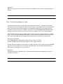
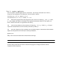
We patch up a delay line with two unit delays and three taps with independently adjustable gains
as in Figure 1. In the first exercise you will set these gains to given values, and observe the
output when the input is a single pulse (more exactly, a periodic sequence of single pulses). This
is an important preliminary as it introduces the unit pulse response.
+
OUTPUT
INPUT
b2
b1
b0
UNIT
DELAY
UNIT
DELAY
Figure 1a: general block diagram of the system
Next, you will observe the output when a pair of adjacent pulses is used as input. This near
trivial example provides us with a springboard to the general case. It will demonstrate how
convolution operates as an overlapping and superposition of unit pulse responses. A second more
general input sequence is then used to reveal a deeper insight and to provide a vehicle for
setting up the key formulas.
In the remainder of the lab we use sinewaves as inputs. This takes us to the rediscovery of the
special role of sinusoids in linear time-invariant systems.
In the final exercise we carry out and unravel a disappearing act.
It should take you about 40 minutes to complete this experiment.
Pre-requisites:
Familiarization with the SIGEx conventions and general module usage. A brief review of the
operation of the S/H & UNIT DELAY module from SIGEx User Manual. No theory required.
Equipment
•
PC with LabVIEW Runtime Engine software appropriate for the version being used.
•
NI ELVIS 2 or 2+ and USB cable to suit
•
EMONA SIGEx Signal & Systems add-on board
•
Assorted patch leads
•
Two BNC – 2mm leads
Procedure
Part A – Setting up the NI ELVIS/SIGEx bundle
1.
Turn off the NI ELVIS unit and its Prototyping Board switch.
2.
Plug the SIGEx board into the NI ELVIS unit.
Note: This may already have been done for you.
3.
Connect the NI ELVIS to the PC using the USB cable.
4.
Turn on the PC (if not on already) and wait for it to fully boot up (so that it’s ready to
connect to external USB devices).
5.
Turn on the NI ELVIS unit but not the Prototyping Board switch yet. You should observe
the USB light turn on (top right corner of ELVIS unit).The PC may make a sound to indicate that
the ELVIS unit has been detected if the speakers are activated.
6.
Turn on the NI ELVIS Prototyping Board switch to power the SIGEx board. Check that
all three power LEDs are on. If not call the instructor for assistance.
7.
Launch the SIGEx Main VI.
8.
When you’re asked to select a device number, enter the number that corresponds with
the NI ELVIS that you’re using.
9.
You’re now ready to work with the NI ELVIS/SIGEx bundle.
10.
Select the EXPT 5 tab on the SIGEx SFP.
Note: To stop the SIGEx VI when you’ve finished the experiment, it’s preferable to use the
STOP button on the SIGEx SFP itself rather than the LabVIEW window STOP button at the
top of the window. This will allow the program to conduct an orderly shutdown and close the
various DAQmx channels it has opened.
Experiment
Part 1 – Setting up
11.
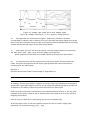
Patch up the model as shown in Figure 2.
Settings are as follows:
PULSE GENERATOR: FREQUENCY=1000Hz; DUTY CYCLE: 0.5 (50%)
SEQUENCE GENERATOR: DIPS UP/UP
SCOPE: Timebase 10ms; Rising edge trigger on CH0; Trigger level=1V
+
OUTPUT
INPUT
b2
b1
b0
UNIT
DELAY
UNIT
DELAY
Figure 1b: general block diagram of the system
Figure 2: patching diagram of the system in Figure 1
12.
The required signal appears at the SEQUENCE GENERATOR SYNC output as a 5V signal
and needs to be reduced in amplitude using the available a0 GAIN function . Using the scope,
check that you have a periodic sequence of a single 1V pulse in a frame of 31 pulse periods.
Confirm the pulse width is 1ms. Adjust the a0 gain value to have a pulse amplitude of 1V
precisely. Adjust the SCOPE trig level to suit.
Note that as the incoming pulse is being clocked by the same clock as the unit delay blocks, the
pulse is already aligned with the unit delay clock and is thus already a discrete signal. For this
reason it can be input directly into the unit delay without use of the S/H block.
Part 2 – unit pulse response
Before proceeding with the examination of the system response, the delay line “tap” gains must
be set. For the first case we shall use b0 = 0.3, b1 = 0.5 and b2 = 0.2 (see Figure 1). These
settings have been chosen arbitrarily as interesting and varied values for this exercise. Adjust
each gain in turn on the SFP and use the scope to confirm your settings.
Question 1
Describe a procedure for confirming the GAIN at each tap ?
Question 2
Display the delay line input signal (i.e. at the first z-1 block input) and the ADDER output signal.
Measure and record the amplitude of each pulse in the output sequence.
Note that the system output is a sequence of three contiguous pulses with amplitudes in the
same ratio as the adder input gains. Could this have been predicted from Figure 1?
Indeed, since the single pulse at the input is generating delayed and scaled replicas as it travels
down the delay line. These are then summed in the adder.
Thus we have the system’s response to an isolated pulse. From this we can define the unit pulse
response h(n) as the response when the amplitude of the input pulse is unity.
From your measurements, show that the unit pulse h(0) = b0 , h(1) = b1 , h(2) = b2 in this
example.
The presence of delayed energy is normally expected in real-life systems, whether electrical or
mechanical. For example, due to inertia in mechanical systems. Similarly in electric circuits, we
have energy storage effects in reactive components such as capacitors and inductors.
Part 3 – The superposition sum
13.
Adjust the SEQUENCE GENERATOR DIP switches to position UP:DOWN to select the
sequence of two contiguous pulses. Using the same gain settings as in Part 2, observe the output
signal. Note that it consists of four nonzero pulses per frame. Measure and record the
amplitude of each pulse.
14.
Verify that the output sequence is simply the sum of two offset unit pulse responses.
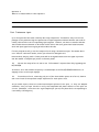
Use the graph below to show your computation.
Graph 1: unit pulse pair summation
Question 3
What is meant by “superposition”. Discuss how this exercise above relates to superposition and
the “additivity” principle.
Question 4
What do you expect to see if this exercise were expanded to two or more contiguous pulses ?
Explain.
Part 4:rectified sinewave at input
In this exercise the input is a little more interesting than in Part 3: a sequence of three or
four pulses of different amplitude. We obtain the source of this signal from the ANALOG OUT
DAC-0. We then pass this analog signal to the SAMPLE/HOLD block to be sampled and this
becomes our discrete sequence of pulses. Note that the PULSE GENERATOR and DAC signal
generator share the same internal clock and hence no slippage occurs in the scope displays.
Note that although the signal is sampled and becomes “discrete” it has not become a “digital”
signal. This is an important distinction. Rather it now exists as sequential discrete samples of
the original signal. More about sampling and its implications in several later experiments.
Settings are as follows:
PULSE GENERATOR: FREQUENCY=800Hz; DUTY CYCLE: 0.5 (50%)
SCOPE: Timebase 10ms; Rising edge trigger on CH0; Trigger level=1V
Confirm that the sinewave from the DAC-0 is 100Hz, 2V peak, before entering the RECTIFIER.
We will treat the sinewave as a continuous signal and ignore the very small steps present as
these have no consequence to our procedure.
Question 5
Note the amplitude of the half wave rectified sine and explain why its amplitude is reduced
relative to the input ?
Figure 3: Block diagram of system with series of pulses as input.
Figure 4: SIGEx patching model for rectified sinewave input
15.
Maintaining the same values for the b gains as in Part 1 (i.e. b0 = 0.3, b1 = 0.5 and b2 = 0.2), display the input (i.e., SAMPLE-HOLD output as shown in Figure 5a) and output signals.
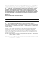
Sketch the original half-rectified sinusoid and discrete output from the SAMPLE/HOLD in the
graph below.
Graph 2: inputs and sampled outputs
Confirm that there are 8 samples of each half wave sine input. This is expected as the sampling
clock is 800Hz and the input sinewave is 100 Hz.
Note there are four nonzero pulses in the delay line input sequence and six in the summer
output. The reason for this will emerge as we proceed.
Again, we will carry out a deconstruction of the output signal in terms of the time offset
contributions, i.e. we will trace the output pulse amplitudes in terms of the
input values. We could use the same method as in Part 3, however, there is an
interesting alternative. We will separately observe and compare the three individual
contributions into the output ADDER, i.e. the signals added through gains b0, b1 and
b2 in turn. Examples of these signals are shown in Figure 5b below.
Figure 5a: example input signal and 4-level sampled signal
Figure 5b: example individual bo, b1 & b2 inputs to adding junction
16.
We begin with the contribution through b2. Temporarily disconnect the leads
corresponding to inputs b0 and b1. Observe and record the input and output signals in the graph
above. Confirm for yourself that this result is as expected. View the sampled input on one scope
channel and the individual output on the other scope channel.
17.
Now repeat for the b1 and b0 contributions. Only the outputs need be recorded since
the same input is used. Again, verify that the results are as expected.
When completed, you will have three scaled replicas of the input with time offsets.
18.
For each time slot, sum the contributions of the three output records and plot the
result. Verify that this agrees with the output signal produced when the three leads are
reconnected to the adder inputs.
Question 6
How does this process relate to the principle of “superposition” ?
In summary, we have just passed a sequence of discrete values (our sampled input) through a
system with a particular response (a series of unit delays with multiplying taps) to produce an
accumulation ( the adder) of discrete product terms which are then output.
Each one of these individual contributions is the scaled and shifted version of the unit pulse
response of this system. Another way of thinking about this system as as it being a series of
weighting coefficients.
Now we need to think about representing this process mathematically.
An obvious way to start is to write a separate formula for the six nonzero output pulse
amplitudes . Let us name them y(1), y(2), …, y(6).
19.
Label them on your sketch above. Pay attention to the orientation you use.
Each consists of a sum of three products, i.e., of a tap gain b0, b1, or b2 and an input pulse
amplitude.
The input sequence has eight elements (as previously observed, four of these are zero). Label
these x(1), x(2), …, x(8) (you should find it convenient to choose x(1) = x(2) = x(7) = x(8) = 0).
20.
Label these on your sketch above.
Numeric indexing is useful as an aid in looking for the general pattern.
The next step is to use symbolic indexing so that the set of formulas can be condensed into one.
Here are some of the formulas as they appear with numeric indexing:
y(3) = b0 .x(3) + b1 .x(2) + b2 .x(1)
y(4) = b0 .x(4) + b1 .x(3) + b2 .x(2)
y(5) = b0 .x(5) + b1 .x(4) + b2 .x(3)
y(6) = b0 .x(6) + b1 .x(5) + b2 .x(4)
Question 7
Write down the formula for y(2) and y(1) ? Discuss any unexpected differences .
The general pattern is readily apparent. With symbolic indexing, we can replace these with the
single formula
y(n) = b0 .x(n) + b1 .x(n -1) + b2 .x(n - 2)
where n represents the position in the sequence as a discrete time index.
In Part 2, we found that the unit pulse response h(k) for this system is
h(0) = b0 , h(1) = b1 , h(2) = b2 .
Hence we can express the formula for y(n) as
y(n) = h(0) .x(n) + h(1).x(n - 1) + h(2).x(n - 2)
i.e.,
y(n) = sum over range of k {h(k).x(n - k)}
This simple formula is known as convolution.
For the discrete signal case we have implemented it is also known as the convolution sum or the
superposition sum. It can also be expressed in this more compact form:
y(n) =
y(n) = x(n) * h(n) where * represents the “convolution” operator.
It provides a neat way of packaging the procedures you carried out in your investigation, and it
allows the range of k to be extended to any desired value. It is the mathematical representation
of the interaction between the input sequence and the unit pulse response of the system.
Note in particular the term x(n-k). Since we are computing in terms of k, this is a time reversed
version of x(k). This issue is put into context further in a later experiment introducing
correlation, an operation which has a similar looking equation. This subject is covered in detail in
the text by Oppenheimer p90 (see Reference section for details)
Question 8
Explain why this term is reversed and what does this mean ?
For the continuous signal case, the summation is achieved using integration and is known as the
convolution integral or the superposition integral. This topic is covered in detail in many texts
including Lathi and Oppenheimer. (see Reference section for details)
In brief, the convolution integral for continuous signals comes about by increasing the number
of discrete samples whilst reducing their width to a limit of 0, such that the sum of many
products can be represented by the integration of the product.
Its equation is
y(t) =
In the above exercise, we obtained the result by means of a superposition of dissected parts of
the unit pulse response. In Part 3 we also used superposition; however, it did not involve
breaking up the unit pulse response. This method was easier to apply for that case because the
input sequence had only two pulses.
Compare the two methods when used with the input in Part 4 (do this with the help of sketch
graphs as before). Consider possible advantages of one over the other as a vehicle for deriving
the convolution formula.
21.
Repeat this process with a new system response. Let each tap be equal to 0.333 ie:
b0=b1=b2=0.333.
Question 9
What is a common label for this response ?
Part 5:sinewave input
Up to this point we have used relatively short input sequences. This made it easy to trace the
passage of the pulses through the system since output segments remained distinct and could be
readily referenced to the corresponding input segment. However, we need to consider whether
the formula that we obtained on this basis is also valid in the more general and usual situation
when the input signal is an ongoing stream without breaks.
For this purpose we will go over the steps in Part 4 using a sinewave as input. This means there
is no "natural" reference marker, hence you will need to designate one.
Nevertheless, keeping track of time points will be straightforward since the signal is periodic
and the number of samples per period is relatively small.
22.
We use the setup in Part 4, and re-use “full sinewave” output at DAC-0 by bypassing the
RECTIFIER.
As before, since the sinewave frequency is a submultiple of the PULSE GENERATOR clock, no
slippage occurs in the scope displays.
23.
Proceed as in Part 4, connecting only one of the three adder inputs. As in Part 4, observe
and record each of the separate output sequences for each input in turn.
As you would expect, these are scaled and delayed replicas of the input, i.e. they are sampled
sinewaves. Carry out spot checks to verify that amplitude and phase relative to the input are
correct. (Reminder, since there are eight samples per period, the phase shift corresponding to
a unit delay is 45 degrees.)
24.
For each time slot, add up the contributions of the three output records obtained above
and plot the result. Verify that this agrees with the output signal produced when all the input
leads are reconnected to the adder.
Graph 3: sinewave input signals
Now we are ready to revisit the formula obtained in Part 4. Proceed as before and show that
the formula remains valid for this case.
Question 10
Show that the formula remains valid.
This completes the basics of the convolution formula.
In the next task we take a closer look at the output signal obtained in Part 5, and show that it is
a sampled sinewave. This is a discrete-time example of the investigation in Lab 4, where we
discovered that when the input of a linear system is sinusoidal, the output will also be sinusoidal.
25.
Confirm that the eight pulses making up one period of the output sequence represent
samples of a sinewave. A straightforward method is to exploit the sum of squares identity.
Since there are eight samples per period, you can match pairs of samples that are 90 degrees
apart (how many pairs can you find?). Note that knowledge of the peak amplitude is not essential
for this (all that is needed is to show that the sum of the squares is the same for each pair).
Question 11
Show your working for the sum of squares analysis ?
26.
Use the FUNCTION GENERATOR tuned to 100 Hz to provide the alternative
unsynchronized sinewave input. Set it to an amplitude of 2Vpeak (4V pp). The resulting slippage
effectively produces an interpolation of the samples -- a useful exploitation of something that
is usually unwanted!
Now that we have a simple way of displaying the input and output sinewaves, an interesting
additional item to examine is the theoretical verification of the measured output/input
amplitude ratio and phase shift. The peak values are clearly apparent, so the amplitude ratio
measurement is straightforward. Similarly, the now discernible zero crossings can be used for
the phase shift measurement.
The math for the theoretical verification is done by means of the application of the formula for
reducing the sum of sinusoids .
In the next Part we investigate an example of effects that can be obtained by means of suitably
chosen values for the tap gains.
Part 6: mystery application
Here we explore a special application of convolution. The setup is the same as for Part 5,
except for new tap gains in the delay line. Two sets will be tested.
The first is b0 = 0.3 , b1 = 0.424 , b2 = 0.3
The second set is b0 = -0.3 , b1 = 0.424 , b2 = -0.3
27.
When the tap gains have been adjusted to the first set of values,( b0 = 0.3 , b1 = 0.424 ,
b2 = 0.3), display the output, and measure the amplitude and phase relative to the input as in
Part 5. Confirm that this is in agreement with theory.
28.
Alter the tap values to the second set of values (b0 = -0.3 , b1 = 0.424 , b2 = -0.3) and
repeat the measurements. Is the outcome predicted by theory ?
29.
Vary the frequency of the sinewave over a suitable range to demonstrate that sinewave
inputs with frequencies near 100 Hz are heavily attenuated.
Question 12
Why is the outcome obtained above described as filtering?
In other labs you will discover how to choose the tap gains to design different kinds of
responses versus frequency.
Tutorial questions
Q1
Look up your textbook to find out the name given to systems that have the structure
in Figure 1, i.e. without feedback. Consider an alternative discrete-time
system that has a single delay element with feedback (refer to your textbook
if needed). Show how to apply the convolution formula in this case.
Q2 Consider the condition(s) required to avoid infinite output values in applications
where the unit pulse response is not time limited. Show to avoid an unstable
output in the feedback system in Q1.
Q3 Consider a process that consists of taking a running average of a data sequence, such
as atmospheric pressure. Suppose we do this by taking the sum of 50% of the
middle value, and 25% of the preceding and following values. Can this process
be described as convolution? If so, write down the unit pulse response.
Q4 Using integration instead of discrete summation, write down a continuous-time
version of the convolution formula in terms of the system impulse response.