Download Experiment # 3 Fast Fourier Transform

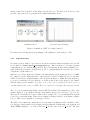
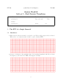
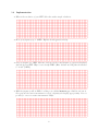
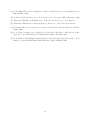
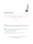
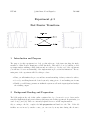
c
2006
Bruno Korst-Fagundes
ECE 431
Fall 2006
Experiment # 3
Fast Fourier Transform
−→
1
−→
Introduction and Purpose
The purpose for this experiment is to lead you through some of the issues involving the implementation of Fast Fourier Transforms on DSP hardware. This will be done by building a crude
spectrum analyzer utilizing a DSP platform and an oscilloscope. By the end of the experiment,
you will have a better understanding of the implementation process and its limitations. The two
main parts of the experiment will follow this procedure:
• First, you will simulate the process, and have an understanding of what you intend to achieve;
• Second, you will implement the desired system by using given code and making sure it runs;
• Finally, you will change parameters within the system as well as the input signal and analyze
the resulting output.
2
Background Reading and Preparation
The bibliography at the end of this outline contains a list of good sources for you to better understand the mathematical and practical issues which may arise in this experiment. In particular, you
can look at [5] and [29]. These are extremely helpful references on DSP implementation.
Before coming to the lab, complete the lab preparation and hand it to the T.A.. If the lab
facilities are not in use by another course, you can come by at any time during office hours to
1
practice. It is beneficial for you, even for your future professional practice, to become acquainted
with the tools and equipment in this lab.
3
Experiment
The experiment is divided into two main parts. On the first part you will simulate and implement
a system which performs an FFT on a single sinusoid for a given number of FFT points. Following
that, you will simulate and implement a similar system, having now two sinusoids as input and
different numbers of FFT points. Your objective on this second part of the experiment will be
to actually display two sinusoids on the scope by making the right decision regarding the FFT
resolution. In sum, you are building a very crude spectrum analyzer with your DSP platform and
your oscilloscope.
All results are to be reported in the spaces provided in this outline. Make sure that
the T.A. verifies every result you record.
3.1
The FFT of a Single Sinusoid
Since you have already played extensively with Matlab in the last experiment, this time you will
simulate a running system in Simulink and verify the changes in output for variations on the input
frequency and amplitude.
3.1.1
Simulation
The system to be implemented is very straight-forward: the input is a sinusoid (time domain) and
the output is the magnitude FFT of it (frequency domain). Bring Matlab and Simulink up and
open a new model. You will create a simple system with a discrete-time sine (called a DSP Sine
Wave), a Buffer block, a Magnitude FFT block and a Vector Scope block. Since the FFT is an
operation performed on frames of data, it is necessary for you to store incoming data in a buffer
prior to calculating the FFT. This same procedure also takes place for the actual implementation
of an FFT on the DSP platform. Your system should look like the one presented in Figure 1
For this simulation, you will only display the magnitude of your calculated sequence, even though
the output of the FFT is a set of complex numbers yielding magnitude and phase information. Set
the buffer size (double click on the Buffer block) to 64, and the number of points on the Magnitude
FFT block to 64. As a general rule, always set the buffer with the same number as the FFT points.
If the buffer is smaller, the simulation will produce an error; if it is larger, the display will interpret
the size of the buffer as reference for the frequency axis.
Set the Vector Scope options to “Input Domain: Frequency”. Feel free to change the display
mode to whatever you feel is better to answer the questions and report the results. You can also
set the running time from 10.0 to inf, so that the simulation runs continuously and you can change
some of the parameters while the system is running.
Now set the sinusoid to 6KHz, 1Vpp . Run the system (click on the “play” icon). Your system
2
and the result yielded should look like Figure 1(b) shown below. The little circle at the tip of the
spectral component is set by going under the channels/markers menu.
(a) Simulation Model
(b) Frequency Domain Display
Figure 1: Simulation of FFT for a Single Sinusoid
Now answer the following questions pertaining to the simulation on the answer booklet.
3.1.2
Implementation
Now that you know what to expect from your system, run Code Composer Studio and open the
project named c:/ECE431/Exp03 FFT/FFT64/FFT64.pjt. Take a moment to look at the programs
comprising the project implementing an FFT. Try to identify important routines within the program, such as the generation of twiddle factors, the loop implementing the butterflies, the location
of input and output buffers, etc.
Make sure you connect inputs and outputs to the instruments. Set the signal generator to a 2KHz,
1Vpp sinusoid. Set the output impedance of the generator to High Z. Compile the project and make
it run. You should see a display similar to the one shown in Figure 2. Adjust the horizontal sweep
to provide you with the best view (like the one in the picture), and set the trigger to the channel
with the single periodic impulse. Note this: your scope is set to display time domain, but it is
actually displaying the result of an FFT. This is to say that it is displaying the frequency domain!
The code you are running implements a 64 point FFT in real-time. The magnitude portion of the
result is displayed on one channel, while the other channel only provides a reference, or a “beacon”.
This reference is actually the location of DC on the very first “bin” of your resulting FFT, and will
be used for your measurements. This reference impulse is displayed as the bottom signal on Figure
2 above. This reference impulse is your trigger reference.
The DSP board continuously outputs the block of 64 numbers resulting from the calculation. Since
you only have a single sinusoid as your input, and it is within the Nyquist limit, your output should
display TWO “impulses”: one between DC and F2s and the other between F2s and Fs . All other
3
Figure 2: Oscilloscope Display For Single Sinusoid Input
values are close to zero, as there is no other spectral component. Since this happens continuously,
you will see more than two impulses on you scope. However, the period that you are interested in
happens between two DC (or reference) spikes. You have studied the cyclical nature of the Fourier
Transform. The scope is actually displaying repeated versions of the same results. Though it looks
the same as your textbook picture for the Fourier Transform, the interval calculated is from DC to
Fs . The results are displayed back to back, repeatedly. This is to say that between two reference
“DC” spikes you will have the interval from DC to Fs .
For a better understanding of what is happening, increase the frequency of the sinusoid from 2KHz
to 10KHz. When you see the peaks moving you know which channel is displaying the magnitude
of your sinusoid. Place the frequency back at 2KHz and the magnitude at 1Vpp .
On some of the questions you will be required to measure the frequency displayed on the scope.
Since you have references at DC and Fs , your best option will be to use cursors to find the time
difference between one of the references and your desired signal. A simple calculation will yield
the frequency value. Feel free to adjust the horizontal span of your scope to provide you with a
better picture. The relative time value between cursors is displayed on the right side under the
label Delta. The picture you should see on the scope is displayed in Figure 3. Answer the questions
pertaining to the implementation on the answer booklet.
3.2
FFT Resolution for Two Sinusoids
Now your objective is to establish a good enough length for the FFT to resolve a more complex
signal. In a practical setting, this would be analogous to selecting the resolution of the spectrum
analyzer to view, say, a carrier signal modulated in amplitude by a sinusoid.
As you know by now, a greater number of FFT points will increase the resolution in the frequency
domain, since it decreases the spaces between adjacent frequency points. In other words, the
resulting sequence has a greater number of “bins” for the same frequency interval.
4
Figure 3: Oscilloscope Display For Cursor Measurement
3.2.1
Simulation
Add one DSP Sine and one Product to the previous system you simulated, so that your system
will look like the one on Figure 4 below. Set one of the sinusoids to be 6KHz and the other 500Hz.
Your Buffer and FFT blocks should be set to 64 still. Run your simulation. While you run it, you
will notice that the curve will move; the picture displayed on Figure 4 is a snapshot of the running
system. Run the system and answer the questions.
(a) Simulation Model
(b) Frequency Domain (wrong) Display
Figure 4: Simulation of FFT for Two Sinusoids
3.2.2
Implementation
The arbitrary signal generators which you have on your workstation allow for signals to be designed
or recorded, and then loaded on to the generator. The signal you will utilize in this part of the
5
experiment is under the function button labelled Arb on the generators.
After you select the appropriate signal, make sure your output button is pressed or no signal will
be input to the DSP. Your objective here is to find the components of your input signal.
Since the workstations have two types of signal generators, the signal you will use in this part of
the experiment has been downloaded onto the instrument. Set the generator as directed by the lab
personnel.
Start Code Composer Studio and load the project c:/ECE431/Exp03 FFT/FFT256/FFT256.pjt
onto it. Compile and run the project. Make sure you have an output displayed on the scope.
Answer the questions.
4
Conclusion
In this experiment, you simulated and implemented a Fast Fourier Transform algorithm, and tested
its limitations for different input signals. You have likely verified that for a greater number of FFT
points, a finer frequency resolution is achieved. This is done at the cost of greater memory use
(to store longer input and output sequences), and greater processing time, which depending on
your real-time constraints may pose as an impediment to long FFT calculations. Since the FFT
algorithm by its very nature is fast, processing time may be lengthened by multiple external memory
reads to retrieve buffered input data and write output data. On your next experiment you will
simulate and implement different digital filter topologies.
6
c
2006
Bruno Korst-Fagundes
ECE 431
Fall 2006
Answer Booklet
Lab # 3 - Fast Fourier Transform
• Name:
Experiment Date:
• Student No.:
Day of the week:
Time:
• Name:
• Student No.:
1
Grade:
/ 25
The FFT of a Single Sinusoid
1.1
Simulation
• What is the resolution presented to you by the scope? How would you improve the resolution?
What is the cost of improving the resolution of your calculated FFT?
• Present a calculation for the amplitude value. Is the simulated amplitude right? If you change
the frequency of the sinusoid to 1KHz, what happens and why?
7
1.2
Implementation
• What is the resolution of your FFT? Show the rather simple calculation.
• Move your frequency up to 27KHz. Explain what happened and why.
• Set your frequency to 5KHz. Measure (and report) the actual frequency component displayed
after the 64 point FFT. Why is it not exactly 5KHz? (Hint: between two DC peaks the interval
is “worth” 48KHz)
• With the frequency still at 5KHz, load the project labeled FFT1024.pjt. Build it and run it.
Now perform the same measurement as above, adjusting the display appropriately. Does it
provide for a more accurate measurement? Why?
8
2
FFT Resolution for Two Sinusoids
2.1
Simulation
• Draw what you would expect to see in the frequency domain as a result of one 6KHz sinusoid
multiplied by one 500Hz sinusoid. Explain why you would expect that.
• Why is the display not showing what you exected to see? (hint: this has nothing to do with
the acual display)
• If you increase the number of points of the FFT will you solve the problem? What size would
you consider acceptable? Are the amplitudes values what you expected? What are the ones
expected?
9
2.2
Implementation
• Draw the output displayed on the scope. Use cursors as a tool to calculate the frequency in
which it is located, and present your calculation. What appears to be this signal?
• Change the project to c:/ECE431/Exp03 FFT/FFT1024/FFT1024.pjt. Compile and run it,
without changing the input. Draw the output displayed on the scope. What appears to be this
signal?
• Use the FFT capability of the oscilloscope to confirm your findings.
10
References
[1] Agilent Technologies, Agilent 33220A - 20MHz Function Arbitrary Waveform Generator User’s Guide Agilent Technologies, Inc. 2003
[2] A. Bateman, Digital Communications - Design for the Real World, Addison-Wesley
[3] A. Bateman, I. Paterson-Stephens, The DSP Handbook - Algorithms, Applications and Design
Techniques, Prentice Hall, 2004
[4] R. Chassaing, DSP Applications Using C and the TMS320c6x DSK, Wiley, 2002
[5] R. Chassaing, Digital Signal Processing and Applications with the c6713 and c6416 DSK, Wiley,
2004
[6] J. B. Dabney and T. L. Harman, Mastering Simulink, Pearson Prentice Hall, 2004
[7] N. Dahnoun, Digital Signal Processing Implementation - Using the TMS320c6000 DSP Platform
Prentice Hall, 2000
[8] P. Embree, C Algorithms for Real-Time DSP, Prentice Hall, 1995
[9] I. Glover and P. Grant, Digital Communications, Prentice Hall, 1998
[10] S. Haykin, Communication Systems, 4th Edition. Toronto: John Wiley & Sons, Inc., 2001.
[11] E. Ifeachor and B. Jervis, Digital Signal Processing - A Practical Approach, Addison Wesley
[12] N. Ketharnavaz, Real-Time Digital Signal Processing, Elsevier, 2004
[13] S. M. Kuo and B. H. Lee, Real-Time Digital Signal Processing - Implementations, Applications
and Experiments with the TMS320c55x, Wiley, 2001
[14] S. M. Kuo, B. H. Lee and W. Tian, Real-Time Digital Signal Processing - Implementations
and Applications - 2nd Ed., Wiley, 2006
[15] P. Kumar, Digital Signal Processing Laboratory, CRC Press, 2005
[16] B. P. Lathi, Modern Digital and Analog Communication Systems, 3rd Edition. New York:
Oxford University Press, 1998.
[17] The Mathworks, Inc., Using Simulink.
[18] The Mathworks, Inc., Real-Time Workshop.
[19] A. V. Oppenheim, A. S. Willsky, with S. H. Nawab, Signals and Systems, 2nd Edition, Prentice
Hall, 1996
[20] A. V. Oppenheim, R. W. Schaeffer, Discrete-Time Signal Processing, Prentice Hall, 1989
[21] S. Orfanidis, Introduction to Signal Processing, Prentice Hall
[22] K. V. Rangarao and R. K. Mallik, Digital Signal Processing - A Practitioner’s Approach Wiley,
2005
11
[23] S. W. Smith, The Scientist and Engineer’s Guide to Digital Signal Processing, Analog Devices,
1999 (available online)
[24] J. Stein, Digital Signal Processing - A Computer Science Perspective, Wiley Interscience 2000
[25] Tektronix, TDS1000 and TDS2000 Series Digital Storage Oscilloscope - User Manual
[26] Tektronix, AFG3000 Series Arbitrary/Function Generators - Quick Start User Manual
[27] W.Tomasi, Electronic Communication Systems, Fundamentals Through Advanced, 2nd Ed.,
Prentice Hall
[28] S. A. Tretter, Communication System Design Using DSP Algorithms - With Laboratory Experiments for the TMS320c6701 and TMS320c6711, Kluwer Academic, 2003
[29] T. B. Welch, C. H. G. Wright and M. G. Morrow, Real-Time Digital Signal Processing - From
Matlab to C with the TMS320C6X DSK, CRC Press, Taylor & Francis, 2006
12