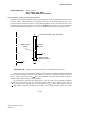
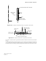
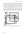
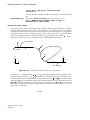
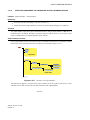
Download Abaqus Analysis User`s Manual, vol1

Abaqus Analysis User’s Manual
Abaqus Version 6.6 ID:
Printed on:
Abaqus Analysis
User’s Manual
Volume I
Version 6.8
Abaqus Version 6.6 ID:
Printed on:
Legal Notices
CAUTION: This documentation is intended for qualified users who will exercise sound engineering judgment and expertise in the use of the Abaqus
Software. The Abaqus Software is inherently complex, and the examples and procedures in this documentation are not intended to be exhaustive or to apply
to any particular situation. Users are cautioned to satisfy themselves as to the accuracy and results of their analyses.
Dassault Systèmes and its subsidiaries, including Dassault Systèmes Simulia Corp., shall not be responsible for the accuracy or usefulness of any analysis
performed using the Abaqus Software or the procedures, examples, or explanations in this documentation. Dassault Systèmes and its subsidiaries shall not
be responsible for the consequences of any errors or omissions that may appear in this documentation.
DASSAULT SYSTÈMES AND ITS SUBSIDIARIES DISCLAIM ALL EXPRESS OR IMPLIED REPRESENTATIONS AND WARRANTIES,
INCLUDING ANY IMPLIED WARRANTY OF MERCHANTABILITY OR FITNESS FOR A PARTICULAR PURPOSE OF THE CONTENTS OF
THIS DOCUMENTATION.
IN NO EVENT SHALL DASSAULT SYSTÈMES, ITS SUBSIDIARIES, OR THEIR THIRD-PARTY PROVIDERS BE LIABLE FOR ANY INDIRECT,
INCIDENTAL, PUNITIVE, SPECIAL, OR CONSEQUENTIAL DAMAGES (INCLUDING, WITHOUT LIMITATION, DAMAGES FOR LOSS
OF BUSINESS PROFITS, BUSINESS INTERRUPTION, OR LOSS OF BUSINESS INFORMATION) EVEN IF DASSAULT SYSTÈMES OR ITS
SUBSIDIARY HAS BEEN ADVISED OF THE POSSIBILITY OF SUCH DAMAGES.
The Abaqus Software is available only under license from Dassault Systèmes or its subsidiary and may be used or reproduced only in accordance with the
terms of such license.
This documentation and the software described in this documentation are subject to change without prior notice.
No part of this documentation may be reproduced or distributed in any form without prior written permission of Dassault Systèmes or its subsidiary.
Export and re-export of the Abaqus Software and this documentation is subject to United States and other export control regulations. Each user is responsible
for compliance with applicable export regulations.
The Abaqus Software is a product of Dassault Systèmes Simulia Corp., Providence, RI, USA.
© Dassault Systèmes, 2008
Printed in the United States of America.
U.S. GOVERNMENT USERS: The Abaqus Software and its documentation are “commercial items,” specifically “commercial computer software” and
“commercial computer software documentation” and, consistent with FAR 12.212 and DFARS 227.7202, as applicable, are provided with restricted rights
in accordance with license terms.
Abaqus, the 3DS logo, SIMULIA, and CATIA are trademarks or registered trademarks of Dassault Systèmes or its subsidiaries in the United States and/or
other countries.
Other company, product, and service names may be trademarks or service marks of their respective owners. For additional information
concerning trademarks, copyrights, and licenses, see the Legal Notices in the Abaqus Version 6.8 Release Notes and the notices at:
http://www.simulia.com/products/products_legal.html.
Abaqus Version 6.6 ID:
Printed on:
Offices and Representatives
SIMULIA Worldwide Headquarters
SIMULIA European Headquarters
Rising Sun Mills, 166 Valley Street, Providence, RI 02909–2499, Tel: +1 401 276 4400,
Fax: +1 401 276 4408, [email protected], http://www.simulia.com
Gaetano Martinolaan 95, P. O. Box 1637, 6201 BP Maastricht, The Netherlands, Tel: +31 43 356 6906,
Fax: +31 43 356 6908, [email protected]
Sales, Support, and Services
North America
Argentina
Australia
Austria
Benelux
Brazil
Czech Republic
France
Germany
India
Israel
Italy
Japan
Korea
Malaysia
New Zealand
Poland
Russia, Belarus & Ukraine
Scandinavia
Singapore
South Africa
Spain
Taiwan
Thailand
Turkey
United Kingdom
Abaqus Version 6.6 ID:
Printed on:
Central, West Lafayette, IN, Tel: +1 765 497 1373, [email protected]
Central, Cincinnati, West Chester, OH, Tel: +1 513 275 1430, [email protected]
Central, Minneapolis/St. Paul, Woodbury, MN, Tel: +1 612 424 9044, [email protected]
East, Warwick, RI, Tel: +1 401 739 3637, [email protected]
Erie, Beachwood, OH, Tel: +1 216 378 1070, [email protected]
Great Lakes, Northville, MI, Tel: +1 248 349 4669, [email protected]
South, Lewisville, TX, Tel: +1 972 221 6500, [email protected]
West, Fremont, CA, Tel: +1 510 794 5891, [email protected]
Dassault Systèmes Latin America, Buenos Aires, Tel: +54 11 4345 2360, [email protected]
Dassault Systèmes Australia Pty. Ltd., Richmond VIC, Tel: +61 3 9421 2900, [email protected]
Vienna, Tel: +43 1 929 16 25-0, [email protected]
Huizen, The Netherlands, Tel: +31 35 52 58 424, [email protected]
SMARTtech Mecânica, São Paulo SP, Tel: +55 11 3168 3388, [email protected]
SMARTtech Mecânica, Rio de Janeiro RJ, Tel: + 55 21 3852 2360, [email protected]
Synerma s. r. o., Psáry, Tel: +420 603 145 769, [email protected]
Versailles, Tel: +33 1 39 24 15 40, [email protected]
Aachen, Tel: +49 241 474010, [email protected]
München, Tel: +49 89 5434 8770, [email protected]
Teynampet, Chennai, Tel: +91 44 65651590, [email protected]
ADCOM, Givataim, Tel: +972 54 6830290, [email protected]
Italy, Milano, Tel: +39 02 39211211, [email protected]
Tokyo, Tel: +81 3 5474 5817, [email protected]
Osaka, Tel: +81 6 4803 5020, [email protected]
Mapo-Gu, Seoul, Tel: +82 2 785 6707, [email protected]
WorleyParsons Advanced Analysis, Kuala Lumpur, Tel: +60 3 2161 2266, [email protected]
Matrix Applied Computing Ltd., Auckland, Tel: +64 9 623 1223, [email protected]
BudSoft Sp. z o.o., Sw. Marcin, Tel: +48 61 8508 466, [email protected]
TESIS Ltd., Moscow, Russia, Tel: +7 495 612 4422, [email protected]
Västerås, Sweden, Tel: +46 21 150870, [email protected]
WorleyParsons Advanced Analysis, Singapore, Tel: +65 6735 8444, [email protected]
Finite Element Analysis Services (Pty) Ltd., Mowbray, Tel: +27 21 448 7608, [email protected]
Principia Ingenieros Consultores, S.A., Madrid, Tel: +34 91 209 1482, [email protected]
APIC, Taipei, Tel: +886 02 25083066, [email protected]
WorleyParsons Advanced Analysis Group, Bangkok, Tel: +66 2 689 3000, [email protected]
A-Ztech Ltd., Istanbul, Tel: +90 216 361 8850, [email protected]
Sevenoaks, Kent, Tel: +44 1 925 830900, [email protected]
Warrington, Tel: +44 1 925 830900, [email protected]
Sales Only
North America
Finland
India
Great Lakes Canada, Toronto, ON, Canada, Tel: +1 416 402 2219, [email protected]
East, Mid-Atlantic, Forest Hill, MD, Tel: +1 410 420 8587, [email protected]
South, Southeast, Acworth, GA, Tel: +1 770 795 0960, [email protected]
West, Southern CA and AZ, Tustin, CA, Tel: +1 714 731 5895, [email protected]
West, Rocky Mountains, Boulder, CO, Tel: +1 303 664 5444, [email protected]
Vantaa, Tel: +358 9 2517 8157, [email protected]
New Delhi, Tel: +91 11 55171877, [email protected]
Pune, Tel: +91 20 32913739, [email protected]
China Representative Offices
China
Chaoyang District, Beijing, P. R. China, Tel: +86 10 65362345, [email protected]
Rudong District, Shanghai, P. R. China, Tel: +86 21 5888 0101, [email protected]
Complete contact information is available at http://www.simulia.com/about/locations.html.
Abaqus Version 6.6 ID:
Printed on:
Preface
This section lists various resources that are available for help with using Abaqus.
Support
Both technical engineering support (for problems with creating a model or performing an analysis) and
systems support (for installation, licensing, and hardware-related problems) for Abaqus are offered through
a network of local support offices. Contact information is listed in the front of each Abaqus manual.
SIMULIA Online Support System
The SIMULIA Online Support System (SOSS) has a knowledge database of SIMULIA Answers. The
SIMULIA Answers are solutions to questions that we have had to answer or guidelines on how to use
Abaqus. You can also submit new requests for support in the SOSS. All support incidents are tracked in the
SOSS. If you are contacting us by means outside the SOSS to discuss an existing support problem and you
know the incident number, please mention it so that we can consult the database to see what the latest action
has been.
To use the SOSS, you need to register with the system. Visit the My Support page at www.simulia.com
for instructions on how to register.
Many questions about Abaqus can also be answered by visiting the Products page and the Support
page at www.simulia.com.
Anonymous ftp site
Useful documents are maintained on an anonymous ftp account on the computer ftp.simulia.com. Login as
user anonymous, and type your e-mail address as your password.
Training
All offices offer regularly scheduled public training classes. We also provide training seminars at customer
sites. All training classes and seminars include workshops to provide as much practical experience with
Abaqus as possible. For a schedule and descriptions of available classes, see www.simulia.com or call your
local representative.
Feedback
We welcome any suggestions for improvements to Abaqus software, the support program, or documentation.
We will ensure that any enhancement requests you make are considered for future releases. If you wish to
make a suggestion about the service or products, refer to www.simulia.com. Complaints should be addressed
by contacting your local office or through www.simulia.com.
Abaqus Version 6.6 ID:
Printed on:
CONTENTS
Contents
Volume I
PART I
1.
INTRODUCTION, SPATIAL MODELING, AND EXECUTION
Introduction
Introduction
Introduction: general
1.1.1
Abaqus syntax and conventions
Input syntax rules
Conventions
1.2.1
1.2.2
Defining an Abaqus model
Defining a model in Abaqus
1.3.1
Parametric modeling
Parametric input
2.
1.4.1
Spatial Modeling
Defining nodes
Node definition
Parametric shape variation
Nodal thicknesses
Normal definitions at nodes
Transformed coordinate systems
2.1.1
2.1.2
2.1.3
2.1.4
2.1.5
Defining elements
Element definition
Element foundations
Defining reinforcement
Defining rebar as an element property
Orientations
2.2.1
2.2.2
2.2.3
2.2.4
2.2.5
Defining surfaces
Surfaces: overview
Defining element-based surfaces
Defining node-based surfaces
Defining analytical rigid surfaces
2.3.1
2.3.2
2.3.3
2.3.4
vii
Abaqus ID:usb-toc
Printed on: Mon March 10 -- 15:15:22 2008
CONTENTS
Defining Eulerian surfaces
Operating on surfaces
2.3.5
2.3.6
Defining rigid bodies
Rigid body definition
2.4.1
Defining integrated output sections
Integrated output section definition
2.5.1
Defining nonstructural mass
Nonstructural mass definition
2.6.1
Defining distributions
Distribution definition
2.7.1
Defining display bodies
Display body definition
2.8.1
Defining an assembly
Defining an assembly
2.9.1
Defining matrices
Defining matrices
3.
2.10.1
Execution Procedures
Execution procedures: overview
Execution procedure for Abaqus: overview
3.1.1
Execution procedures
Execution procedure for obtaining information
Execution procedure for Abaqus/Standard and Abaqus/Explicit
Execution procedure for Abaqus/CAE
Execution procedure for Abaqus/Viewer
Execution procedure for Python
Execution procedure for parametric studies
Execution procedure for Abaqus HTML documentation
Execution procedure for licensing utilities
Execution procedure for ASCII translation of results (.fil) files
Execution procedure for joining results (.fil) files
Execution procedure for querying the keyword/problem database
Execution procedure for fetching sample input files
Execution procedure for making user-defined executables and subroutines
Execution procedure for input file and output database upgrade utility
Execution procedure for generating output database reports
viii
Abaqus ID:usb-toc
Printed on: Mon March 10 -- 15:15:22 2008
3.2.1
3.2.2
3.2.3
3.2.4
3.2.5
3.2.6
3.2.7
3.2.8
3.2.9
3.2.10
3.2.11
3.2.12
3.2.13
3.2.14
3.2.15
CONTENTS
Execution procedure for joining output database (.odb) files from restarted analyses
Execution procedure for combining output from substructures
Execution procedure for network output database file connector
Execution procedure for fixed format conversion utility
Execution procedure for translating NASTRAN bulk data files to Abaqus input files
Execution procedure for translating Abaqus input files to NASTRAN bulk data files
Execution procedure for translating PAM-CRASH input files to partial Abaqus input
files
Execution procedure for translating RADIOSS input files to partial Abaqus input files
Execution procedure for translating Abaqus output database files to NASTRAN
Output2 results files
Execution procedure for exchanging Abaqus data with ZAERO
Execution procedure for encrypting and decrypting Abaqus input data
Execution procedures for job execution control
3.2.16
3.2.17
3.2.18
3.2.19
3.2.20
3.2.21
3.2.22
3.2.23
3.2.24
3.2.25
3.2.26
3.2.27
Environment file settings
Using the Abaqus environment settings
3.3.1
Managing memory and disk resources
Managing memory and disk use in Abaqus
3.4.1
File extension definitions
File extensions used by Abaqus
3.5.1
FORTRAN unit numbers
FORTRAN unit numbers used by Abaqus
3.6.1
PART II
4.
OUTPUT
Output
Output
Output
Output to the data and results files
Output to the output database
4.1.1
4.1.2
4.1.3
Output variables
Abaqus/Standard output variable identifiers
Abaqus/Explicit output variable identifiers
4.2.1
4.2.2
The postprocessing calculator
The postprocessing calculator
4.3.1
ix
Abaqus ID:usb-toc
Printed on: Mon March 10 -- 15:15:22 2008
CONTENTS
5.
File Output Format
Accessing the results file
Accessing the results file: overview
Results file output format
Accessing the results file information
Utility routines for accessing the results file
OI.1
Abaqus/Standard Output Variable Index
OI.2
Abaqus/Explicit Output Variable Index
5.1.1
5.1.2
5.1.3
5.1.4
x
Abaqus ID:usb-toc
Printed on: Mon March 10 -- 15:15:22 2008
CONTENTS
Volume II
PART III
6.
ANALYSIS PROCEDURES, SOLUTION, AND CONTROL
Analysis Procedures
Introduction
Procedures: overview
General and linear perturbation procedures
Multiple load case analysis
Direct linear equation solver
Iterative linear equation solver
Static stress/displacement analysis
6.1.1
6.1.2
6.1.3
6.1.4
6.1.5
Static stress analysis procedures: overview
Static stress analysis
Eigenvalue buckling prediction
Unstable collapse and postbuckling analysis
Quasi-static analysis
Direct cyclic analysis
Low-cycle fatigue analysis using the direct cyclic approach
Dynamic stress/displacement analysis
6.2.1
6.2.2
6.2.3
6.2.4
6.2.5
6.2.6
6.2.7
Dynamic analysis procedures: overview
Implicit dynamic analysis using direct integration
Explicit dynamic analysis
Direct-solution steady-state dynamic analysis
Natural frequency extraction
Complex eigenvalue extraction
Transient modal dynamic analysis
Mode-based steady-state dynamic analysis
Subspace-based steady-state dynamic analysis
Response spectrum analysis
Random response analysis
Steady-state transport analysis
6.3.1
6.3.2
6.3.3
6.3.4
6.3.5
6.3.6
6.3.7
6.3.8
6.3.9
6.3.10
6.3.11
Steady-state transport analysis
Heat transfer and thermal-stress analysis
6.4.1
Heat transfer analysis procedures: overview
Uncoupled heat transfer analysis
Sequentially coupled thermal-stress analysis
6.5.1
6.5.2
6.5.3
xi
Abaqus ID:usb-toc
Printed on: Mon March 10 -- 15:15:22 2008
CONTENTS
Fully coupled thermal-stress analysis
Adiabatic analysis
6.5.4
6.5.5
Electrical analysis
Electrical analysis procedures: overview
Coupled thermal-electrical analysis
Piezoelectric analysis
6.6.1
6.6.2
6.6.3
Coupled pore fluid flow and stress analysis
Coupled pore fluid diffusion and stress analysis
Geostatic stress state
6.7.1
6.7.2
Mass diffusion analysis
Mass diffusion analysis
6.8.1
Acoustic and shock analysis
Acoustic, shock, and coupled acoustic-structural analysis
6.9.1
Abaqus/Aqua analysis
Abaqus/Aqua analysis
6.10.1
Annealing
Annealing procedure
7.
6.11.1
Analysis Solution and Control
Solving nonlinear problems
Solving nonlinear problems
Contact iterations
7.1.1
7.1.2
Analysis convergence controls
Convergence and time integration criteria: overview
Commonly used control parameters
Convergence criteria for nonlinear problems
Time integration accuracy in transient problems
PART IV
8.
7.2.1
7.2.2
7.2.3
7.2.4
ANALYSIS TECHNIQUES
Analysis Techniques: Introduction
Analysis techniques: overview
8.1.1
xii
Abaqus ID:usb-toc
Printed on: Mon March 10 -- 15:15:22 2008
CONTENTS
9.
Analysis Continuation Techniques
Restarting an analysis
Restarting an analysis
9.1.1
Importing and transferring results
Transferring results between Abaqus analyses: overview
Transferring results between Abaqus/Explicit and Abaqus/Standard
Transferring results from one Abaqus/Standard analysis to another
Transferring results from one Abaqus/Explicit analysis to another
10.
9.2.1
9.2.2
9.2.3
9.2.4
Modeling Abstractions
Substructuring
Using substructures
Defining substructures
10.1.1
10.1.2
Submodeling
Submodeling: overview
Node-based submodeling
Surface-based submodeling
10.2.1
10.2.2
10.2.3
Generating global matrices
Generating global matrices
10.3.1
Symmetric model generation, results transfer, and analysis of cyclic symmetry models
Symmetric model generation
Transferring results from a symmetric mesh or a partial three-dimensional mesh to
a full three-dimensional mesh
Analysis of models that exhibit cyclic symmetry
10.4.1
10.4.2
10.4.3
Meshed beam cross-sections
Meshed beam cross-sections
11.
10.5.1
Special-Purpose Techniques
Inertia relief
Inertia relief
11.1.1
Mesh modification or replacement
Element and contact pair removal and reactivation
11.2.1
Geometric imperfections
Introducing a geometric imperfection into a model
xiii
Abaqus ID:usb-toc
Printed on: Mon March 10 -- 15:15:22 2008
11.3.1
CONTENTS
Fracture mechanics
Fracture mechanics: overview
Contour integral evaluation
Crack propagation analysis
11.4.1
11.4.2
11.4.3
Hydrostatic fluid modeling
Modeling fluid-filled cavities
11.5.1
Surface-based fluid modeling
Surface-based fluid cavities: overview
Defining fluid cavities
Defining fluid exchange
Defining inflators
11.6.1
11.6.2
11.6.3
11.6.4
Mass scaling
Mass scaling
11.7.1
Steady-state detection
Steady-state detection
11.8.1
Parallel execution
Parallel execution in Abaqus
Parallel execution in Abaqus/Standard
Parallel execution in Abaqus/Explicit
12.
11.9.1
11.9.2
11.9.3
Adaptivity Techniques
Adaptivity techniques: overview
Adaptivity techniques
12.1.1
ALE adaptive meshing
ALE adaptive meshing: overview
Defining ALE adaptive mesh domains in Abaqus/Explicit
ALE adaptive meshing and remapping in Abaqus/Explicit
Modeling techniques for Eulerian adaptive mesh domains in Abaqus/Explicit
Output and diagnostics for ALE adaptive meshing in Abaqus/Explicit
Defining ALE adaptive mesh domains in Abaqus/Standard
ALE adaptive meshing and remapping in Abaqus/Standard
12.2.1
12.2.2
12.2.3
12.2.4
12.2.5
12.2.6
12.2.7
Adaptive remeshing
Adaptive remeshing: overview
Error indicators
Solution-based mesh sizing
12.3.1
12.3.2
12.3.3
xiv
Abaqus ID:usb-toc
Printed on: Mon March 10 -- 15:15:22 2008
CONTENTS
Analysis continuation after mesh replacement
Mesh-to-mesh solution mapping
13.
12.4.1
Eulerian Analysis
Eulerian analysis
14.
13.1.1
Extending Abaqus Analysis Functionality
Co-simulation
Co-simulation: overview
Preparing an Abaqus analysis for co-simulation
14.1.1
14.1.2
User subroutines and utilities
User subroutines: overview
Available user subroutines
Available utility routines
15.
14.2.1
14.2.2
14.2.3
Design Sensitivity Analysis
Design sensitivity analysis
16.
15.1.1
Parametric Studies
Scripting parametric studies
Scripting parametric studies
16.1.1
Parametric studies: commands
aStudy.combine(): Combine parameter samples for parametric studies
aStudy.constrain(): Constrain parameter value combinations in parametric studies
aStudy.define(): Define parameters for parametric studies
aStudy.execute(): Execute the analysis of parametric study designs
aStudy.gather(): Gather the results of a parametric study
aStudy.generate(): Generate the analysis job data for a parametric study
aStudy.output(): Specify the source of parametric study results
aStudy=ParStudy(): Create a parametric study
aStudy.report(): Report parametric study results
aStudy.sample(): Sample parameters for parametric studies
xv
Abaqus ID:usb-toc
Printed on: Mon March 10 -- 15:15:22 2008
16.2.1
16.2.2
16.2.3
16.2.4
16.2.5
16.2.6
16.2.7
16.2.8
16.2.9
16.2.10
CONTENTS
Volume III
PART V
17.
MATERIALS
Materials: Introduction
Introduction
Material library: overview
Material data definition
Combining material behaviors
17.1.1
17.1.2
17.1.3
General properties
Density
18.
17.2.1
Elastic Mechanical Properties
Overview
Elastic behavior: overview
18.1.1
Linear elasticity
Linear elastic behavior
No compression or no tension
Plane stress orthotropic failure measures
18.2.1
18.2.2
18.2.3
Porous elasticity
Elastic behavior of porous materials
18.3.1
Hypoelasticity
Hypoelastic behavior
18.4.1
Hyperelasticity
Hyperelastic behavior of rubberlike materials
Hyperelastic behavior in elastomeric foams
Anisotropic hyperelastic behavior
18.5.1
18.5.2
18.5.3
Stress softening in elastomers
Mullins effect in rubberlike materials
Energy dissipation in elastomeric foams
18.6.1
18.6.2
Viscoelasticity
Time domain viscoelasticity
Frequency domain viscoelasticity
18.7.1
18.7.2
xvi
Abaqus ID:usb-toc
Printed on: Mon March 10 -- 15:15:22 2008
CONTENTS
Hysteresis
Hysteresis in elastomers
18.8.1
Equations of state
Equation of state
19.
18.9.1
Inelastic Mechanical Properties
Overview
Inelastic behavior
19.1.1
Metal plasticity
Classical metal plasticity
Models for metals subjected to cyclic loading
Rate-dependent yield
Rate-dependent plasticity: creep and swelling
Annealing or melting
Anisotropic yield/creep
Johnson-Cook plasticity
Dynamic failure models
Porous metal plasticity
Cast iron plasticity
Two-layer viscoplasticity
ORNL – Oak Ridge National Laboratory constitutive model
Deformation plasticity
19.2.1
19.2.2
19.2.3
19.2.4
19.2.5
19.2.6
19.2.7
19.2.8
19.2.9
19.2.10
19.2.11
19.2.12
19.2.13
Other plasticity models
Extended Drucker-Prager models
Modified Drucker-Prager/Cap model
Mohr-Coulomb plasticity
Critical state (clay) plasticity model
Crushable foam plasticity models
19.3.1
19.3.2
19.3.3
19.3.4
19.3.5
Fabric materials
Fabric material behavior
19.4.1
Jointed materials
Jointed material model
19.5.1
Concrete
Concrete smeared cracking
Cracking model for concrete
Concrete damaged plasticity
19.6.1
19.6.2
19.6.3
xvii
Abaqus ID:usb-toc
Printed on: Mon March 10 -- 15:15:22 2008
CONTENTS
Permanent set in rubberlike materials
Permanent set in rubberlike materials
20.
19.7.1
Progressive Damage and Failure
Progressive damage and failure: overview
Progressive damage and failure
20.1.1
Damage and failure for ductile metals
Damage and failure for ductile metals: overview
Damage initiation for ductile metals
Damage evolution and element removal for ductile metals
20.2.1
20.2.2
20.2.3
Damage and failure for fiber-reinforced composites
Damage and failure for fiber-reinforced composites: overview
Damage initiation for fiber-reinforced composites
Damage evolution and element removal for fiber-reinforced composites
20.3.1
20.3.2
20.3.3
Damage and failure for ductile materials in low-cycle fatigue analysis
Damage and failure for ductile materials in low-cycle fatigue analysis: overview
Damage initiation for ductile materials in low-cycle fatigue
Damage evolution for ductile materials in low-cycle fatigue
21.
20.4.1
20.4.2
20.4.3
Other Material Properties
Mechanical properties
Material damping
Thermal expansion
21.1.1
21.1.2
Heat transfer properties
Thermal properties: overview
Conductivity
Specific heat
Latent heat
21.2.1
21.2.2
21.2.3
21.2.4
Acoustic properties
Acoustic medium
21.3.1
Hydrostatic fluid properties
Hydrostatic fluid models
21.4.1
Mass diffusion properties
Diffusivity
Solubility
21.5.1
21.5.2
xviii
Abaqus ID:usb-toc
Printed on: Mon March 10 -- 15:15:22 2008
CONTENTS
Electrical properties
Electrical conductivity
Piezoelectric behavior
21.6.1
21.6.2
Pore fluid flow properties
Pore fluid flow properties
Permeability
Porous bulk moduli
Sorption
Swelling gel
Moisture swelling
21.7.1
21.7.2
21.7.3
21.7.4
21.7.5
21.7.6
User materials
User-defined mechanical material behavior
User-defined thermal material behavior
21.8.1
21.8.2
xix
Abaqus ID:usb-toc
Printed on: Mon March 10 -- 15:15:22 2008
CONTENTS
Volume IV
PART VI
22.
ELEMENTS
Elements: Introduction
Element library: overview
Choosing the element’s dimensionality
Choosing the appropriate element for an analysis type
Section controls
23.
22.1.1
22.1.2
22.1.3
22.1.4
Continuum Elements
General-purpose continuum elements
Solid (continuum) elements
One-dimensional solid (link) element library
Two-dimensional solid element library
Three-dimensional solid element library
Cylindrical solid element library
Axisymmetric solid element library
Axisymmetric solid elements with nonlinear, asymmetric deformation
23.1.1
23.1.2
23.1.3
23.1.4
23.1.5
23.1.6
23.1.7
Infinite elements
Infinite elements
Infinite element library
23.2.1
23.2.2
Warping elements
Warping elements
Warping element library
24.
23.3.1
23.3.2
Structural Elements
Membrane elements
Membrane elements
General membrane element library
Cylindrical membrane element library
Axisymmetric membrane element library
24.1.1
24.1.2
24.1.3
24.1.4
Truss elements
Truss elements
Truss element library
24.2.1
24.2.2
Beam elements
Beam modeling: overview
24.3.1
xx
Abaqus ID:usb-toc
Printed on: Mon March 10 -- 15:15:22 2008
CONTENTS
Choosing a beam cross-section
Choosing a beam element
Beam element cross-section orientation
Beam section behavior
Using a beam section integrated during the analysis to define the section behavior
Using a general beam section to define the section behavior
Beam element library
Beam cross-section library
24.3.2
24.3.3
24.3.4
24.3.5
24.3.6
24.3.7
24.3.8
24.3.9
Frame elements
Frame elements
Frame section behavior
Frame element library
24.4.1
24.4.2
24.4.3
Elbow elements
Pipes and pipebends with deforming cross-sections: elbow elements
Elbow element library
24.5.1
24.5.2
Shell elements
Shell elements: overview
Choosing a shell element
Defining the initial geometry of conventional shell elements
Shell section behavior
Using a shell section integrated during the analysis to define the section behavior
Using a general shell section to define the section behavior
Three-dimensional conventional shell element library
Continuum shell element library
Axisymmetric shell element library
Axisymmetric shell elements with nonlinear, asymmetric deformation
25.
24.6.1
24.6.2
24.6.3
24.6.4
24.6.5
24.6.6
24.6.7
24.6.8
24.6.9
24.6.10
Inertial, Rigid, and Capacitance Elements
Point mass elements
Point masses
Mass element library
25.1.1
25.1.2
Rotary inertia elements
Rotary inertia
Rotary inertia element library
25.2.1
25.2.2
Rigid elements
Rigid elements
Rigid element library
25.3.1
25.3.2
xxi
Abaqus ID:usb-toc
Printed on: Mon March 10 -- 15:15:22 2008
CONTENTS
Capacitance elements
Point capacitance
Capacitance element library
26.
25.4.1
25.4.2
Connector Elements
Connector elements
Connectors: overview
Connector elements
Connector actuation
Connector element library
Connection-type library
26.1.1
26.1.2
26.1.3
26.1.4
26.1.5
Connector element behavior
Connector behavior
Connector elastic behavior
Connector damping behavior
Connector functions for coupled behavior
Connector friction behavior
Connector plastic behavior
Connector damage behavior
Connector stops and locks
Connector failure behavior
Connector uniaxial behavior
27.
26.2.1
26.2.2
26.2.3
26.2.4
26.2.5
26.2.6
26.2.7
26.2.8
26.2.9
26.2.10
Special-Purpose Elements
Spring elements
Springs
Spring element library
27.1.1
27.1.2
Dashpot elements
Dashpots
Dashpot element library
27.2.1
27.2.2
Flexible joint elements
Flexible joint element
Flexible joint element library
27.3.1
27.3.2
Distributing coupling elements
Distributing coupling elements
Distributing coupling element library
27.4.1
27.4.2
xxii
Abaqus ID:usb-toc
Printed on: Mon March 10 -- 15:15:22 2008
CONTENTS
Cohesive elements
Cohesive elements: overview
Choosing a cohesive element
Modeling with cohesive elements
Defining the cohesive element’s initial geometry
Defining the constitutive response of cohesive elements using a continuum approach
Defining the constitutive response of cohesive elements using a traction-separation
description
Defining the constitutive response of fluid within the cohesive element gap
Two-dimensional cohesive element library
Three-dimensional cohesive element library
Axisymmetric cohesive element library
27.5.1
27.5.2
27.5.3
27.5.4
27.5.5
27.5.6
27.5.7
27.5.8
27.5.9
27.5.10
Gasket elements
Gasket elements: overview
Choosing a gasket element
Including gasket elements in a model
Defining the gasket element’s initial geometry
Defining the gasket behavior using a material model
Defining the gasket behavior directly using a gasket behavior model
Two-dimensional gasket element library
Three-dimensional gasket element library
Axisymmetric gasket element library
27.6.1
27.6.2
27.6.3
27.6.4
27.6.5
27.6.6
27.6.7
27.6.8
27.6.9
Surface elements
Surface elements
General surface element library
Cylindrical surface element library
Axisymmetric surface element library
27.7.1
27.7.2
27.7.3
27.7.4
Hydrostatic fluid elements
Hydrostatic fluid elements
Hydrostatic fluid element library
Fluid link elements
Hydrostatic fluid link library
27.8.1
27.8.2
27.8.3
27.8.4
Tube support elements
Tube support elements
Tube support element library
27.9.1
27.9.2
Line spring elements
Line spring elements for modeling part-through cracks in shells
Line spring element library
xxiii
Abaqus ID:usb-toc
Printed on: Mon March 10 -- 15:15:22 2008
27.10.1
27.10.2
CONTENTS
Elastic-plastic joints
Elastic-plastic joints
Elastic-plastic joint element library
27.11.1
27.11.2
Drag chain elements
Drag chains
Drag chain element library
27.12.1
27.12.2
Pipe-soil elements
Pipe-soil interaction elements
Pipe-soil interaction element library
27.13.1
27.13.2
Acoustic interface elements
Acoustic interface elements
Acoustic interface element library
27.14.1
27.14.2
Eulerian elements
Eulerian elements
Eulerian element library
27.15.1
27.15.2
User-defined elements
User-defined elements
User-defined element library
EI.1
Abaqus/Standard Element Index
EI.2
Abaqus/Explicit Element Index
27.16.1
27.16.2
xxiv
Abaqus ID:usb-toc
Printed on: Mon March 10 -- 15:15:22 2008
CONTENTS
Volume V
PART VII
28.
PRESCRIBED CONDITIONS
Prescribed Conditions
Overview
Prescribed conditions: overview
Amplitude curves
28.1.1
28.1.2
Initial conditions
Initial conditions
28.2.1
Boundary conditions
Boundary conditions
28.3.1
Loads
Applying loads: overview
Concentrated loads
Distributed loads
Thermal loads
Acoustic and shock loads
Pore fluid flow
28.4.1
28.4.2
28.4.3
28.4.4
28.4.5
28.4.6
Prescribed assembly loads
Prescribed assembly loads
28.5.1
Predefined fields
Predefined fields
28.6.1
PART VIII
29.
CONSTRAINTS
Constraints
Overview
Kinematic constraints: overview
29.1.1
Multi-point constraints
Linear constraint equations
General multi-point constraints
Kinematic coupling constraints
29.2.1
29.2.2
29.2.3
xxv
Abaqus ID:usb-toc
Printed on: Mon March 10 -- 15:15:22 2008
CONTENTS
Surface-based constraints
Mesh tie constraints
Coupling constraints
Shell-to-solid coupling
Mesh-independent fasteners
29.3.1
29.3.2
29.3.3
29.3.4
Embedded elements
Embedded elements
29.4.1
Element end release
Element end release
29.5.1
Overconstraint checks
Overconstraint checks
29.6.1
PART IX
30.
INTERACTIONS
Defining Contact Interactions
Overview
Contact interaction analysis: overview
30.1.1
Defining contact pairs in Abaqus/Standard
Defining contact pairs in Abaqus/Standard
Contact formulations in Abaqus/Standard
Contact constraint enforcement methods in Abaqus/Standard
Modeling contact interference fits in Abaqus/Standard
Adjusting initial surface positions and specifying initial clearances in Abaqus/Standard
contact pairs
Smoothing contact surfaces in Abaqus/Standard
Removing/reactivating Abaqus/Standard contact pairs
Defining tied contact in Abaqus/Standard
Extending master surfaces and slide lines
Contact modeling if substructures are present
Contact modeling if asymmetric-axisymmetric elements are present
Contact diagnostics in an Abaqus/Standard analysis
Common difficulties associated with contact modeling in Abaqus/Standard
Adjusting contact controls in Abaqus/Standard
30.2.1
30.2.2
30.2.3
30.2.4
30.2.5
30.2.6
30.2.7
30.2.8
30.2.9
30.2.10
30.2.11
30.2.12
30.2.13
30.2.14
Defining general contact in Abaqus/Explicit
Defining general contact interactions in Abaqus/Explicit
Assigning surface properties for general contact in Abaqus/Explicit
xxvi
Abaqus ID:usb-toc
Printed on: Mon March 10 -- 15:15:22 2008
30.3.1
30.3.2
CONTENTS
Assigning contact properties for general contact in Abaqus/Explicit
Contact formulation for general contact in Abaqus/Explicit
Resolving initial overclosures and specifying initial clearances for general contact in
Abaqus/Explicit
Contact controls for general contact in Abaqus/Explicit
30.3.3
30.3.4
30.3.5
30.3.6
Defining contact pairs in Abaqus/Explicit
Defining contact pairs in Abaqus/Explicit
Assigning surface properties for contact pairs in Abaqus/Explicit
Assigning contact properties for contact pairs in Abaqus/Explicit
Contact formulations for contact pairs in Abaqus/Explicit
Adjusting initial surface positions and specifying initial clearances for contact pairs
in Abaqus/Explicit
Common difficulties associated with contact modeling using contact pairs in
Abaqus/Explicit
31.
30.4.1
30.4.2
30.4.3
30.4.4
30.4.5
30.4.6
Contact Property Models
Mechanical contact properties
Mechanical contact properties: overview
Contact pressure-overclosure relationships
Contact damping
Contact blockage
Frictional behavior
User-defined interfacial constitutive behavior
Pressure penetration loading
Interaction of debonded surfaces
Breakable bonds
Surface-based cohesive behavior
31.1.1
31.1.2
31.1.3
31.1.4
31.1.5
31.1.6
31.1.7
31.1.8
31.1.9
31.1.10
Thermal contact properties
Thermal contact properties
31.2.1
Electrical contact properties
Electrical contact properties
31.3.1
Pore fluid contact properties
Pore fluid contact properties
32.
31.4.1
Contact Elements in Abaqus/Standard
Contact modeling with elements
Contact modeling with elements
32.1.1
xxvii
Abaqus ID:usb-toc
Printed on: Mon March 10 -- 15:15:22 2008
CONTENTS
Gap contact elements
Gap contact elements
Gap element library
32.2.1
32.2.2
Tube-to-tube contact elements
Tube-to-tube contact elements
Tube-to-tube contact element library
32.3.1
32.3.2
Slide line contact elements
Slide line contact elements
Axisymmetric slide line element library
32.4.1
32.4.2
Rigid surface contact elements
Rigid surface contact elements
Axisymmetric rigid surface contact element library
33.
32.5.1
32.5.2
Defining Cavity Radiation in Abaqus/Standard
Cavity radiation
33.1.1
xxviii
Abaqus ID:usb-toc
Printed on: Mon March 10 -- 15:15:22 2008
Abaqus Version 6.6 ID:
Printed on:
Part I: Introduction, Spatial Modeling, and
Execution
•
•
•
Chapter 1, “Introduction”
Chapter 2, “Spatial Modeling”
Chapter 3, “Execution Procedures”
Abaqus Version 6.6 ID:
Printed on:
INTRODUCTION
1.
Introduction
Introduction
1.1
Abaqus syntax and conventions
1.2
Defining an Abaqus model
1.3
Parametric modeling
1.4
Abaqus Version 6.6 ID:
Printed on:
INTRODUCTION
1.1
Introduction
•
“Introduction: general,” Section 1.1.1
1.1–1
Abaqus Version 6.6 ID:
Printed on:
INTRODUCTION
1.1.1
INTRODUCTION: GENERAL
Overview of the Abaqus finite element system
The Abaqus finite element system includes:
•
•
•
•
Abaqus/Standard, a general-purpose finite element program;
Abaqus/Explicit, an explicit dynamics finite element program;
Abaqus/CAE, an interactive environment used to create finite element models, submit Abaqus
analyses, monitor and diagnose jobs, and evaluate results; and
Abaqus/Viewer, a subset of Abaqus/CAE that contains only the postprocessing capabilities of the
Visualization module.
Several add-on options are available to further extend the capabilities of Abaqus/Standard and
Abaqus/Explicit.
The Abaqus/Aqua, Abaqus/Design, and Abaqus/AMS options work with
Abaqus/Standard. Abaqus/Aqua contains optional features that are specifically designed for the analysis
of beam-like structures installed underwater and subject to loading by water currents and wave action.
The Abaqus/Design option enables you to perform design sensitivity analysis (DSA). Abaqus/AMS is an
optional eigensolver that works within Abaqus/Standard providing very fast solution of large symmetric
eigenvalue problems. The Abaqus co-simulation technique provides several applications, available
as separate add-on capabilities, for coupling between Abaqus and third-party analysis programs.
Abaqus/Foundation is an optional subset of Abaqus/Standard that provides more cost-efficient access
to the linear static and dynamic analysis functionality in Abaqus/Standard. These options are available
only if your license includes them.
For a comprehensive list of Abaqus products, utilities, and add-on options, see “Abaqus products,”
Section 1.2 of the Abaqus Release Notes.
Overview of this manual
This manual is a reference guide to using Abaqus/Standard (including Abaqus/Aqua, Abaqus/Design,
and Abaqus/Foundation) and Abaqus/Explicit. Abaqus/Standard solves a system of equations implicitly
at each solution “increment.” In contrast, Abaqus/Explicit marches a solution forward through time in
small time increments without solving a coupled system of equations at each increment (or even forming
a global stiffness matrix). Throughout the manual the term Abaqus is used to refer collectively to both
Abaqus/Standard and Abaqus/Explicit; the individual product names are used when information applies
to only one product. Product identifiers appear at the beginning of each section in the manual (excluding
overview sections) indicating the products to which the information in the section applies.
The manual is divided into several parts:
•
Part I, “Introduction, Spatial Modeling, and Execution,” discusses basic modeling concepts in
Abaqus, such as defining nodes, elements, and surfaces; the conventions and input formats that
1.1.1–1
Abaqus Version 6.6 ID:
Printed on:
INTRODUCTION
•
•
•
•
•
•
•
•
should be followed when using Abaqus; and the execution procedures for Abaqus/Standard,
Abaqus/Explicit, Abaqus/CAE, and several utilities that are provided with the Abaqus system.
Part II, “Output,” describes how to obtain output from Abaqus and the format of the results (.fil)
file. It also describes the output variable identifiers that are available.
Part III, “Analysis Procedures, Solution, and Control,” describes the analysis types (static stress
analysis, dynamics, eigenvalue extraction, etc.) that are available. Detailed discussions of the
differences between how Abaqus/Standard and Abaqus/Explicit solve finite element analyses are
provided in this chapter.
Part IV, “Analysis Techniques,” discusses various analysis techniques available in Abaqus such as
submodeling, removing elements or surfaces, and importing results from a previous simulation to
define the initial conditions for the current model.
Part V, “Materials,” describes the material modeling options and how to calibrate some of the more
advanced material models.
Part VI, “Elements,” describes the elements available in Abaqus.
Part VII, “Prescribed Conditions,” describes the use of prescribed conditions, such as distributed
loads and nodal velocities.
Part VIII, “Constraints,” discusses the use of constraints, such as multi-point constraints.
Part IX, “Interactions,” discusses the contact and interaction models available in Abaqus.
The manual also includes indexes of all of the output variables and elements available in Abaqus/Standard
and Abaqus/Explicit.
Using Abaqus
Abaqus/Standard and Abaqus/Explicit can be run as batch applications (see “Execution procedure
for Abaqus/Standard and Abaqus/Explicit,” Section 3.2.2, for details) or through the interactive
Abaqus/CAE environment (see “Execution procedure for Abaqus/CAE,” Section 3.2.3, for details
on how to start Abaqus/CAE). The main input to the Abaqus/Standard and Abaqus/Explicit analysis
products is a file containing the options required for the simulation and the data associated with those
options. There may also be supplementary files, such as restart or results files from previous analyses,
or auxiliary data files, such as a file containing an acceleration record or an earthquake record for
dynamic analysis. The input file is usually created by Abaqus/CAE or another preprocessor. Both input
file usage and Abaqus/CAE usage information are provided in this manual.
As described in “Defining a model in Abaqus,” Section 1.3.1, the main input file consists of two
sections: model input and history input. The input is organized around a few natural concepts and
conventions, which means that even though input files for complex simulations can be large, they can
be managed without difficulty. The basic syntax rules that govern an Abaqus input file are discussed
in “Input syntax rules,” Section 1.2.1. The Abaqus Keywords Reference Manual contains a complete
description of all the input options available in Abaqus. For a detailed introduction to using Abaqus for
your analyses, it is recommended that you follow the self-paced tutorials in Getting Started with Abaqus:
Interactive Edition. Refer to the Abaqus/CAE User’s Manual for detailed information on working with
Abaqus/CAE.
1.1.1–2
Abaqus Version 6.6 ID:
Printed on:
INTRODUCTION
In addition, many analyses that demonstrate the numerous capabilities of Abaqus are discussed in
the Abaqus Example Problems Manual, the Abaqus Benchmarks Manual, and the Abaqus Verification
Manual. As a supplement to the Abaqus Analysis User’s Manual, these examples can help you become
familiar with the functionality that Abaqus provides and the structure of the Abaqus input file. For
example, “Beam impact on cylinder,” Section 1.6.10 of the Abaqus Verification Manual, discusses the
various modeling techniques that can be used to analyze the dynamic response of a cantilever beam.
Reviewing the results of an Abaqus simulation
Information on requesting output from an Abaqus simulation is discussed in “Output,” Section 4.1.1.
Requested results from an Abaqus simulation are viewed through the Visualization module in
Abaqus/CAE (also licensed separately as Abaqus/Viewer). The output database file is read by the
Visualization module in Abaqus/CAE to create contour plots, animations, X–Y plots, and tabular output
of Abaqus results. See Part V, “Viewing results,” of the Abaqus/CAE User’s Manual for detailed
information on using the Visualization module in Abaqus/CAE.
1.1.1–3
Abaqus Version 6.6 ID:
Printed on:
Abaqus SYNTAX AND CONVENTIONS
1.2
Abaqus syntax and conventions
•
•
“Input syntax rules,” Section 1.2.1
“Conventions,” Section 1.2.2
1.2–1
Abaqus Version 6.6 ID:
Printed on:
INPUT SYNTAX RULES
1.2.1
INPUT SYNTAX RULES
Products: Abaqus/Standard
Abaqus/Explicit
Reference
•
“Defining a model in Abaqus,” Section 1.3.1
Overview
This section describes the syntax rules that govern an Abaqus input file.
All data definitions in Abaqus are accomplished with option blocks—sets of data describing a part
of the problem definition. You choose those options that are relevant for a particular application. Options
are defined by lines in the input file. Three types of input lines are used in an Abaqus input file: keyword
lines, data lines, and comment lines. A carriage return is required at the end of each line in an input file.
•
•
•
Keyword lines introduce options and often have parameters, which appear as words or phrases
separated by commas on the keyword line. Parameters are used to define the behavior of an option.
Parameters can stand alone or have a value, and they may be required or optional.
Data lines, which are used to provide numeric or alphanumeric entries, follow most keyword lines.
Any line that begins with stars in columns 1 and 2 (**) is a comment line. Such lines can be placed
anywhere in the file. They are ignored by Abaqus, so they will be printed only in the initial listing
of the file. There is no restriction on how many or where such lines occur in the file.
Relevant parameters and data lines (including the number of entries per data line) are described in the
sections of the Abaqus Keywords Reference Manual describing each option. This section describes the
general rules that apply to all keyword and data lines.
Keyword lines
The following rules apply when entering a keyword line:
•
•
•
•
•
•
•
•
The first non-blank character of each keyword line must be a star (*).
The keyword must be followed by a comma (,) if any parameters are given.
Parameters must be separated by commas.
Blanks on a keyword line are ignored.
A line can include no more than 256 characters, including blanks.
Keywords and parameters are not case sensitive.
Parameter values usually are not case sensitive. The only exceptions to this rule are those imposed
externally to Abaqus, such as file names on case-sensitive operating systems.
Keywords, parameters, and, in most cases, parameter values need not be spelled out completely,
but there must be enough characters given to distinguish them from other keywords, parameters,
and parameter values that begin in the same way. Abaqus first searches each associated text string
1.2.1–1
Abaqus Version 6.6 ID:
Printed on:
INPUT SYNTAX RULES
for an exact match. If an exact match is not found, Abaqus then searches based upon the minimum
number of unique characters in each keyword, parameter, or parameter value, as the case may be.
Embedded blanks can be omitted from any item in a keyword line. If a parameter value is used to
provide a number or a file name, the complete value should be provided.
•
If a parameter has a value, the equal sign (=) is used. The value can be an integer, a floating point
number, or a character string, depending on the context. For example,
*ELASTIC, TYPE=ISOTROPIC, DEPENDENCIES=1
•
The same parameter should not appear more than once on a single keyword line. If a parameter has
multiple settings on a single keyword line, Abaqus ignores all but one of the settings.
•
Continuation of a keyword line is sometimes necessary; for example, because of a large number
of parameters. If the last character on a keyword line is a comma, the next line is interpreted as a
continuation of the line. For example, the *ELASTIC keyword line above could also be given as
*ELASTIC, TYPE=ISOTROPIC,
DEPENDENCIES=1
•
Certain keywords must be used in conjunction with other keywords; for example, the *ELASTIC
and *DENSITY keywords must be used in conjunction with the *MATERIAL keyword. These
related keywords must be grouped in a block in the input file; unrelated keywords cannot be specified
within this block.
•
Some options allow the INPUT or FILE parameter to be set equal to the name of an alternate file.
Such file names can include a full path name or a relative path name. Relative path names must be
with respect to the directory from which the job was submitted. If no path is specified, the file is
assumed to be in the directory from which the job was submitted. A substructure library must be in
the same directory from which the job was submitted; a full path name cannot be used to specify a
substructure library name.
For files referenced by the INPUT parameter, the file name must include any extension (e.g.,
elem.inp). For files referenced by the FILE parameter, the name must be given without an
extension in most cases since Abaqus assumes that the file to be read has the correct extension
for the file type that is relevant to the option: .res for restart files (“Restarting an analysis,”
Section 9.1.1) and .fil for results files (“Output,” Section 4.1.1). However, special rules may
apply when a results file (.fil) or an output database file (.odb) is relevant for the option
(see “Initial conditions,” Section 28.2.1, and “Sequentially coupled thermal-stress analysis,”
Section 6.5.3, for details).
The file or substructure library name must have the correct case on computers with casesensitive operating systems. Regardless of whether the user specifies only a file name, a relative
path name, or a full path name, the complete name including the path can have a maximum of
80 characters.
1.2.1–2
Abaqus Version 6.6 ID:
Printed on:
INPUT SYNTAX RULES
Data lines
Data lines are used to provide data that are more easily given in lists than as parameters on an option.
Most options require one or more data lines; if they are required, the data lines must immediately follow
the keyword line introducing the option. The following rules apply when entering a data line:
•
•
•
•
•
A data line can include no more than 256 characters, including blanks. Trailing blanks are ignored.
All data items must be separated by commas (,). An empty data field is specified by omitting data
between commas. Abaqus will use values of zero for any required numeric data that are omitted
unless a default value is specified. If a data line contains only a single data item, the data item should
be followed by a comma to distinguish the data line from a fixed format data line used in previous
versions of Abaqus.
A line must contain only the number of items specified.
Empty data fields at the end of a line can be ignored.
Floating point numbers can occupy a maximum of 20 spaces including the sign, decimal point, and
any exponential notation.
Floating point numbers can be given with or without an exponent. Any exponent, if input,
must be preceded by E or D and an optional (−) or (+). The following line shows four acceptable
ways of entering the same floating point number:
-12.345
•
•
•
-1234.5E-2
-1234.5D-2
-1.2345E1
Integer data items can occupy a maximum of 9 digits.
Character strings can be up to 80 characters long and are not case sensitive.
Continuation lines are allowed in specific instances (see “Element definition,” Section 2.2.1). If
allowed, such lines are indicated by a comma as the last character of the preceding line. A single
data item cannot be entered over multiple lines.
In many cases the choice of parameters used with an option determines the type of data lines required. For
example, there are five different ways to define a linear elastic material (“Elastic behavior: overview,”
Section 18.1.1). The data lines you specify must be consistent with the value of the TYPE parameter
given on the *ELASTIC option.
Sets
One of the most useful features of the Abaqus data definition method is the availability of sets. A set can
be a set of nodes or a set of elements. You provide a name (1–80 characters, the first of which must be a
letter) for each set. That name then provides a means of referencing all of the members of the set. As an
example suppose that, for the structure shown in Figure 1.2.1–1, we wish to apply symmetry boundary
conditions at all of the nodes in the set MIDDLE and that the edge SUPPORT is pinned. We assemble the
relevant nodes into sets and specify the boundary conditions by
*BOUNDARY
MIDDLE, ZSYMM
SUPPORT, PINNED
1.2.1–3
Abaqus Version 6.6 ID:
Printed on:
INPUT SYNTAX RULES
NSET middle
NSET support
y
x
z
Figure 1.2.1–1
Example of the use of sets.
Sets are the basic reference throughout Abaqus, and the use of sets is recommended. Choosing
meaningful set names makes it simple to identify which data belong to which part of the model.
Further discussion of sets is provided in “Node definition,” Section 2.1.1, and “Element definition,”
Section 2.2.1.
Labels
Labels such as set names, surface names, and rebar names are case insensitive (except when they are
accessed from user subroutines; see “User subroutines: overview,” Section 14.2.1) and can be up to
80 characters long. All spaces within a label are ignored unless the label is enclosed in quotation marks,
in which case all spaces within the label are maintained. A label that is not enclosed within quotation
marks must begin with a letter, may not include a period (.), and should not contain characters such
as commas and equal signs. These restrictions do not apply to labels enclosed within quotation marks
except if the label is a material name. A material name must always start with a letter, even if the name
is enclosed within quotation marks.
If a label is defined using quotation marks, the quotation marks are stored as part of the label. Any
subsequent use of the label should also be enclosed in quotation marks. Embedded quotation marks are
not allowed.
1.2.1–4
Abaqus Version 6.6 ID:
Printed on:
INPUT SYNTAX RULES
Labels cannot begin and end with a double underscore (e.g., __STEEL__). This label format is
reserved for internal use by Abaqus.
The following are examples of labels entered with and without the use of quotation marks:
*ELEMENT, TYPE=SPRINGA, ELSET="One element"
1,1,2
*SPRING, ELSET="One element"
1.0E-5,
*NSET, ELSET="One element", NSET=NODESET
*BOUNDARY
nodeset,1,2
Repeating data lines
Some options list only a single data line. In cases where only one data line is allowed, this is indicated
by the data line title “First (and only) line.” An example of this is the *DYNAMIC option. In many cases
the single data line shown can be repeated to define one variable as a function of another; this choice is
indicated by a note after the data line. For example, a table of biaxial test data can be given to define a
hyperelastic material:
*BIAXIAL TEST DATA
,
,
,
Etc.
There is no limit on the number of data lines allowed, but the data must be given in a certain order, as
explained below.
Many options require more than one data line; these are indicated by the data line titles “First line:”,
“Second line:”, etc. For example, exactly two data lines must be used to define a local orientation for a
shell element (*ORIENTATION), and at least three data lines are required to define anisotropic elasticity
(*ELASTIC).
In many cases the data lines can be repeated, which is indicated by a note after the data lines. As
with repetition of a single data line, it is important that sets of data lines be given in the correct order so
that Abaqus can interpolate the data properly.
Example: Multiple data lines due to field variable dependence
Any time an option can be defined as a function of field variables, you must determine the number of data
lines required to define the option completely. (See “Specifying field variable dependence” in “Material
data definition,” Section 17.1.2, for more information.) For example, two data lines are required if stressbased failure criteria (*FAIL STRESS) are defined as a function of two field variables. This pair of data
lines is repeated as often as necessary to define the failure criteria completely:
1.2.1–5
Abaqus Version 6.6 ID:
Printed on:
INPUT SYNTAX RULES
*FAIL STRESS, DEPENDENCIES=2
second
pair
third
pair
⎫
⎬
⎭
⎫
⎬
⎭
⎫
⎬
⎭
first
pair
X1t , X1c , Y1t , Y1c, S1,
fv11, fv12
, σ1biax
X2t , X2c , Y2t , Y2c, S2,
fv12, fv22
, σ2biax
X3t , X3c , Y3t , Y3c, S3,
fv31, fv32
, σ3biax
Etc.
(In this example the last field on the first data line of each pair was omitted, which means that the stressbased failure criteria are not temperature dependent.)
If the stress-based failure criteria were defined as a function of nine field variables, a set of three
data lines would be repeated as often as necessary:
first
set
⎫
⎬
⎭
second
set
*FAIL STRESS, DEPENDENCIES=9
X1t , X1c , Y1t , Y1c, S1, , σ1biax
fv11, fv12, fv13, fv14, fv15, fv16, fv71, fv18
fv19
X2t , X2c , Y2t , Y2c, S2, , σ2biax
fv12, fv22, fv23, fv24, fv25, fv62, fv72, fv82
fv29
Etc.
⎫
⎬
⎭
Ordering the data lines
Whenever one variable is defined as a function of another, the data must be given in the proper order so
that Abaqus can interpolate for intermediate values correctly. The variable being defined is assumed to be
constant outside the range of independent variables given, except for nonlinear elastic gasket thickness
behavior involving damage where the data are extrapolated based on the last slope computed from the
user-specified data.
If the property being defined is a function of only one variable (such as the *BIAXIAL TEST DATA
shown above), the data should be given in the order of increasing value of the independent variable.
If the property being defined is a function of multiple independent variables, the variation of the
property with respect to the first variable must be given at fixed values of the other variables, in ascending
values of the second variable, then of the third variable, and so on. The data lines must always be ordered
so that the independent variables are given increasing values. This process ensures that the value of the
1.2.1–6
Abaqus Version 6.6 ID:
Printed on:
INPUT SYNTAX RULES
material property is completely and uniquely defined at any values of the independent variables upon
which the property depends.
As an example, consider isotropic elasticity defined as a function of three field variables (but not of
temperature):
*ELASTIC,
,
,
,
,
,
,
,
,
,
,
,
,
,
,
,
,
,
,
,
,
,
,
,
,
,
,
,
,
,
,
,
,
,
,
,
,
DEPENDENCIES=3
, 1, 1, 1
, 2, 1, 1
, 1, 2, 1
, 2, 2, 1
, 1, 3, 1
, 2, 3, 1
, 1, 1, 2
, 2, 1, 2
, 1, 2, 2
, 2, 2, 2
, 1, 3, 2
, 2, 3, 2
, 1, 1, 3
, 2, 1, 3
, 1, 2, 3
, 2, 2, 3
, 1, 3, 3
, 2, 3, 3
1.2.1–7
Abaqus Version 6.6 ID:
Printed on:
CONVENTIONS
1.2.2
CONVENTIONS
Products: Abaqus/Standard
Abaqus/Explicit
Abaqus/CAE
References
•
•
•
Chapter 2, “Spatial Modeling”
Part II, “Output”
“Boundary conditions,” Section 28.3.1
Overview
The conventions that are used throughout Abaqus are defined in this section. The following topics are
discussed:
•
•
•
•
•
•
•
•
•
Degrees of freedom
Coordinate systems
Self-consistent units
Time measures
Local directions on surfaces in space
Stress and strain conventions
Stress and strain measures in geometrically nonlinear analysis
Conventions for finite rotations
Conventions for tabular data input
Degrees of freedom
Except for axisymmetric elements, the degrees of freedom are always referred to as follows:
1
2
3
4
5
6
7
8
9
10
11
x-displacement
y-displacement
z-displacement
Rotation about the x-axis, in radians
Rotation about the y-axis, in radians
Rotation about the z-axis, in radians
Warping amplitude (for open-section beam elements)
Pore pressure, hydrostatic fluid pressure, or acoustic pressure
Electric potential
Connector material flow (units of length)
Temperature (or normalized concentration in mass diffusion analysis)
1.2.2–1
Abaqus Version 6.6 ID:
Printed on:
CONVENTIONS
12
13
14
Second temperature (for shells or beams)
Third temperature (for shells or beams)
Etc.
Here the x-, y-, and z-directions coincide with the global X-, Y-, and Z-directions, respectively; however,
if a local transformation is defined at a node (see “Transformed coordinate systems,” Section 2.1.5), they
coincide with the local directions defined by the transformation.
A maximum of 20 temperature values (degrees of freedom 11 through 30) can be defined for shell
or beam elements in Abaqus/Standard.
Axisymmetric elements
The displacement and rotation degrees of freedom in axisymmetric elements are referred to as follows:
1
2
5
6
r-displacement
z-displacement
Rotation about the z-axis (for axisymmetric elements with twist), in radians
Rotation in the r–z plane (for axisymmetric shells), in radians
Here the r- and z-directions coincide with the global X- and Y-directions, respectively; however, if a
local transformation is defined at a node (see “Transformed coordinate systems,” Section 2.1.5), they
coincide with the local directions defined by the transformation.
Activation of degrees of freedom
Abaqus activates only those degrees of freedom needed at a node. Thus, some of the degrees of freedom
listed above may not be used at all nodes in a model, because each element type uses only those degrees of
freedom that are relevant. For example, two-dimensional solid (continuum) stress/displacement elements
use only degrees of freedom 1 and 2. The degrees of freedom actually used at any node are the envelope
of those needed in each element that shares the node.
Internal variables in Abaqus/Standard
In addition to the degrees of freedom listed above, Abaqus/Standard uses internal variables (such as
Lagrange multipliers to impose constraints) for some elements. Normally you need not be concerned
with these variables, but they may appear in error and warning messages and are checked for satisfaction
of nonlinear constraints during iteration. Internal variables are always associated with internal nodes,
which have negative numbers to distinguish them from user-defined nodes.
Coordinate systems
The basic coordinate system in Abaqus is a right-handed, rectangular Cartesian system. You can choose
other systems locally for input (see “Node definition,” Section 2.1.1), for output of nodal variables
(displacements, velocities, etc.) and point load or boundary condition specification (see “Transformed
coordinate systems,” Section 2.1.5), and for material or kinematic joint specification (see “Orientations,”
Section 2.2.5). All coordinate systems must be right-handed.
1.2.2–2
Abaqus Version 6.6 ID:
Printed on:
CONVENTIONS
Units
Abaqus has no units built into it except for rotation and angle measures. Therefore, the units chosen must
be self-consistent, which means that derived units of the chosen system can be expressed in terms of the
fundamental units without conversion factors.
Rotation and angle measures
In Abaqus rotational degrees of freedom are expressed in radians, and all other angle measures are
expressed in degrees (for example, phase angles).
International System of units (SI)
The International System of units (SI) is an example of a self-consistent set of units. The fundamental
units in the SI system are length in meters (m), mass in kilograms (kg), time in seconds (s), temperature
in degrees Kelvin (K), and electric current in Amperes (A). The units of secondary or derived quantities
are based on these fundamental units. An example of a derived unit is the unit of force. A unit of force
in the SI system is called a Newton (N):
Newton
kg m s
Similarly, a unit of electrical charge in the SI system is called a Coulomb (C):
Coulomb
As
Another example is the unit of energy, called a Joule (J):
Joule
Nm
A Volt s
kg m s
The unit of electrical potential in the SI system is the Volt, which is chosen such that
Joule
Volt C
Volt A s
Sometimes the standard units are not convenient to work with. For example, Young’s modulus is
frequently specified in terms of MegaPascals (MPa) (or, equivalently, N/mm2 ), where 1 Pascal = 1 N/m2 .
In this case the fundamental units could be tonnes (1 tonne = 1000 kilograms), millimeters, and seconds.
American or English units
American or English units can cause confusion since the naming conventions are not as clear as in the
SI system. For example, 1 pound force (lbf) will give 1 pound mass (lbm) an acceleration of g ft/sec2 ,
where g is the value of acceleration due to gravity. If pounds force, feet (ft), and seconds are taken as
fundamental units, the derived unit of mass is lbf sec2 /ft. Since density is commonly given in handbooks
as lbm/in3 , it must be converted to lbf sec2 /ft4 by
1.2.2–3
Abaqus Version 6.6 ID:
Printed on:
CONVENTIONS
lbm in
lbf sec ft
Frequently it is not made clear in handbooks whether lb stands for lbm or lbf. You need to check that the
values used make up a consistent set of units.
Two other units that cause difficulty are the slug, defined as the mass that will be accelerated at
1 ft/sec2 by 1 lbf, and the poundal, defined as the force required to accelerate 1 lbm at 1 ft/sec2 . Useful
conversions are
slug
lbm
and
lbf
poundals
where g is the magnitude of the acceleration due to gravity in ft/sec2 .
Symbols used in Abaqus for units
Units are indicated for the value to be given on load and flux types as follows:
Dimension
Indicator
Example (S.I. units)
length
L
meter
mass
M
kilogram
time
T
second
degree Celsius
temperature
electric current
A
Ampere
force
F
Newton
energy
J
Joule
electric charge
C
Coulomb
volt
electric potential
mass concentration
P
Parts per million
Time
Abaqus has two measures of time—step time and total time. Except for certain linear perturbation
procedures, step time is measured from the beginning of each step. Total time starts at zero and is the total
accumulated time over all general analysis steps (including restart steps; see “Restarting an analysis,”
Section 9.1.1). Total time does not accumulate during linear perturbation steps.
1.2.2–4
Abaqus Version 6.6 ID:
Printed on:
CONVENTIONS
Local directions on surfaces in space
Local directions are needed on surfaces in space; for example, to define the tangential slip directions on
an element-based contact surface or to define stress and strain components in a shell. The convention
used in Abaqus for such directions is as follows.
The default local 1-direction is the projection of the global x-axis onto the surface. If the global
x-axis is within 0.1° of being normal to the surface, the local 1-direction is the projection of the global
z-axis onto the surface. The local 2-direction is then at right angles to the local 1-direction, so that the
local 1-direction, local 2-direction, and the positive normal to the surface form a right-handed set (see
Figure 1.2.2–1). The positive normal direction is defined in an element by the right-hand rotation rule
going around the nodes of the element. The local surface directions can be redefined; see “Orientations,”
Section 2.2.5.
surface normal
4
2
1
3
1
2
projection of x-axis
onto surface
3
1
2
z
4
2
y
x
Figure 1.2.2–1
1
surface
normal
Default local surface directions.
The local 1- and 2-directions become local 2- and 3-directions, respectively, when considering
gasket elements or the local systems associated with integrated output sections (“Integrated output section
definition,” Section 2.5.1) or user-defined sections (“Section output from Abaqus/Standard” in “Output
to the data and results files,” Section 4.1.2).
1.2.2–5
Abaqus Version 6.6 ID:
Printed on:
CONVENTIONS
For “line”-type surfaces defined on beam, pipe, or truss elements in space, the default local
1-direction and 2-direction are tangential and transverse to the elements. In this case the local surface
directions can also be redefined as described in “Orientations,” Section 2.2.5.
Rotation of the local directions
For geometrically linear analysis, stress and strain components are given by default in the material
directions in the reference (initial) configuration.
For geometrically nonlinear analysis, small-strain shell elements in Abaqus/Standard (S4R5,
S8R, S8R5, S8RT, S9R5, STRI3, and STRI65) use a total Lagrangian strain, and the stress and strain
components are given relative to material directions in the reference configuration. Gasket elements
are small-strain small-displacement elements, and the components are output by default in the behavior
directions in the reference configuration.
For finite-membrane-strain elements (all membrane elements, S3/S3R, S4, S4R, SAX, and SAXA
elements) and for small-strain shell elements in Abaqus/Explicit, the material directions rotate with the
average rigid body motion of the surface to form the material directions in the current configuration.
Stress and strain components in these elements are given relative to these material directions in the
current configuration.
For a more thorough discussion of the definition of the rotated coordinate directions in membrane
elements; S3/S3R, S4, and S4R elements; S3RS, S4RS, and S4RSW elements; and SAXA elements, see:
•
•
•
•
“Membrane elements,” Section 3.4.1 of the Abaqus Theory Manual,
“Finite-strain shell element formulation,” Section 3.6.5 of the Abaqus Theory Manual,
“Small-strain shell elements in Abaqus/Explicit,” Section 3.6.6 of the Abaqus Theory Manual, and
“Axisymmetric shell element allowing asymmetric loading,” Section 3.6.7 of the Abaqus Theory
Manual.
You can determine whether the local system associated with a user-defined section is fixed or rotates
with the average rigid body motion; see “Section output from Abaqus/Standard” in “Output to the data
and results files,” Section 4.1.2, for details.
You can determine whether the local system associated with an integrated output section is fixed,
translates with average rigid body motion, or translates and rotates with the average rigid body motion;
see “Integrated output section definition,” Section 2.5.1, for details.
See “Contact formulations in Abaqus/Standard,” Section 30.2.2, for information on how the slip
directions evolve during an Abaqus/Standard contact analysis.
Convention used for stress and strain components
When defining material properties, the convention used for stress and strain components in Abaqus is
that they are ordered:
Direct stress in the 1-direction
Direct stress in the 2-direction
Direct stress in the 3-direction
Shear stress in the 1–2 plane
1.2.2–6
Abaqus Version 6.6 ID:
Printed on:
CONVENTIONS
Shear stress in the 1–3 plane
Shear stress in the 2–3 plane
For example, a fully anisotropic, linear elasticity matrix is
symm.
The 1-, 2-, and 3-directions depend on the element type chosen. For solid elements the defaults for
these directions are the global spatial directions. For shell and membrane elements the defaults for the
1- and 2-directions are local directions in the surface of the shell or membrane, as defined in Part VI,
“Elements.” In both cases the 1-, 2-, and 3-directions can be changed as described in “Orientations,”
Section 2.2.5.
For geometrically nonlinear analysis with solid elements, the default (global) directions do not rotate
with the material. However, user-defined orientations do rotate with the material.
Abaqus/Explicit stores the stress and strain components internally in a different order:
,
,
,
,
,
. For geometrically nonlinear analysis, the internally stored components rotate with the
material, regardless of whether or not a user-defined orientation is used. This distinction is important
when a user subroutine (such as VUMAT) is used.
Nonisotropic material behavior
When nonisotropic material behavior is defined in continuum elements, a user-defined orientation is
necessary for the anisotropic behavior to be associated with material directions. See “State storage,”
Section 1.5.4 of the Abaqus Theory Manual, for a description of how material directions rotate.
Zero-valued stress components
Stress components that are always zero are omitted from storage. For example, in plane stress Abaqus
stores only the two direct components and one shear component of stress and strain in the plane where
the stress values are nonzero.
Shear strains
Abaqus always reports shear strain as engineering shear strain, :
1.2.2–7
Abaqus Version 6.6 ID:
Printed on:
CONVENTIONS
Stress and strain measures
The stress measure used in Abaqus is Cauchy or “true” stress, which corresponds to the force per
current area. See “Stress measures,” Section 1.5.2 of the Abaqus Theory Manual, and “Stress rates,”
Section 1.5.3 of the Abaqus Theory Manual, for more details on stress measures.
For geometrically nonlinear analysis, a large number of different strain measures exist. Unlike
“true” stress, there is no clearly preferred “true” strain. For the same physical deformation different
strain measures will report different values in large-strain analysis. The optimal choice of strain measure
depends on analysis type, material behavior, and (to some degree) personal preference. See “Strain
measures,” Section 1.4.2 of the Abaqus Theory Manual, for more details on strain measures.
By default, the strain output in Abaqus/Standard is the “integrated” total strain (output variable E).
For large-strain shells, membranes, and solid elements in Abaqus/Standard two other measures of total
strain can be requested: logarithmic strain (output variable LE) and nominal strain (output variable NE).
Logarithmic strain (output variable LE) is the default strain output in Abaqus/Explicit; nominal
strain (output variable NE) can be requested as well. The “integrated” total strain is not available in
Abaqus/Explicit.
Total (integrated) strain
The default “integrated” strain measure, E, output by Abaqus/Standard to the data (.dat) and results
(.fil) files for all elements that can handle finite strain is obtained by integrating the strain rate
numerically in a material frame of reference:
where
and
are the total strains at increments
and n, respectively;
is the incremental
rotation tensor; and
is the total strain increment from increment n to
. For elements that use
a corotational coordinate system (finite-strain shells, membranes, and solid elements with user-defined
orientations), the above equation simplifies to
The strain increment is obtained by integration of the rate of deformation
over the time increment:
This strain measure is appropriate for elastic-(visco)plastic or elastic-creeping materials, because the
plastic strains and creep strains are obtained by the same integration procedure. In such materials the
elastic strains are small (because the yield stress is small compared to the elastic modulus), and the total
strains can be compared directly with the plastic strains and creep strains.
1.2.2–8
Abaqus Version 6.6 ID:
Printed on:
CONVENTIONS
If the principal directions of straining rotate with respect to the material axes, the resulting strain
measure cannot be related to the total deformation, regardless whether a spatial or corotational coordinate
system is used. If the principal directions remain fixed in the material axes, the strain is the integration
of the rate of deformation,
which is equivalent to the logarithmic strain discussed later.
Green’s strain
For small-strain shells and beams in Abaqus/Standard, the default strain measure, E, is Green’s strain:
where is the deformation gradient and is the identity tensor. This strain measure is appropriate for
the small-strain, large-rotation approximation used in these elements. The components of
represent
strain along directions in the original configuration. The small-strain shells and beams should not be
used in finite-strain analysis with either elastic-plastic or hyperelastic material behavior, since incorrect
analysis results may be obtained or program failure may occur.
Nominal strain
The nominal strain, NE, is
where
is the left stretch tensor,
are the principal stretches, and
are the principal
stretch directions in the current configuration. The principal values of nominal strain are, therefore, the
ratios of change in length to length in the reference configuration in the principal directions, thus giving
a direct measure of deformation.
Logarithmic strain
The logarithmic strain, LE, is
where the variables are as defined earlier for nominal strain.
1.2.2–9
Abaqus Version 6.6 ID:
Printed on:
CONVENTIONS
Stress invariants
Many of the constitutive models in Abaqus are formulated in terms of stress invariants. These invariants
are defined as the equivalent pressure stress,
the Mises equivalent stress,
and the third invariant of deviatoric stress,
where
is the deviatoric stress, defined as
Finite rotations
The following convention is used for finite rotations in space: Define , ,
as “rotations” about the
global X, Y, and Z-axes (that is, degrees of freedom 4, 5, and 6 at a node). Then define
where
The direction is then the axis of rotation, and is the angular rotation (in radians) about the axis
according to the right-hand rule (see Figure 1.2.2–2).
The value of is not uniquely determined. In large-rotation problems where the overall rotation
exceeds , any multiple of can be added or subtracted, which may lead to discontinuous output values
for the rotation components. If rotations larger than
about one axis occur in the positive (negative)
direction in Abaqus/Standard, the rotation output varies discontinuously between 0 and
(
). In
Abaqus/Explicit the rotation output varies in all cases between
and .
This convention provides straightforward input of kinematic boundary conditions and moments in
most cases and simple interpretation of the output. The rotations output by Abaqus represent a single
rotation from the reference configuration to the current configuration about a fixed axis. The output does
not follow the history of rotation at a node. In addition, this convention reduces to the usual convention
1.2.2–10
Abaqus Version 6.6 ID:
Printed on:
CONVENTIONS
z
p
Same vector rotated
by ( φx , φy , φz )
φ
y
Initial vector
x
Figure 1.2.2–2
Definition of finite rotation.
for small rotations, even in the case of small rotations superposed on an initial finite rotation (such as
might be considered in the study of small vibrations about a predeformed state).
Compound rotations
Because finite rotations are not additive, the way they must be specified is a bit different from the way
other boundary conditions are specified: the increment in rotation specified over a step must be the
rotation needed to rotate the node from the configuration at the beginning of the step to that desired at
the end of the step. It is not enough to rotate the node over this step to a total rotation vector that would
have taken the node into its final configuration if applied on the node in some other initial reference
configuration. If an increment of rotation
is needed to rotate from the rotation
boundary condition
at the beginning of the step (and at the end of the previous step) to
its final position at the end of the step, the boundary condition must be specified such that the rotation
vector is
at the end of the step. If the direction of the rotation vector
1.2.2–11
Abaqus Version 6.6 ID:
Printed on:
CONVENTIONS
is constant, this method of specifying rotation boundary conditions and the total rotation vector will be
the same.
Example
As an example of how to specify compound finite rotations and to interpret finite rotation output, consider
the following example of the rotation of a beam.
The beam initially lies along the x-axis. We want to perform the compound rotation, where (Step 1)
the beam is rotated by 60° about the z-axis, followed by (Step 2) a 90° spin of the beam about itself,
followed by (Step 3) a 90° rotation of the beam about an axis perpendicular to the beam in the x–y plane,
such that the beam finishes on the z-axis.
This compound rotation is achieved in three steps with applied rotation vectors ,
, and ,
where
For this example
,
, and
. Here
represents the magnitude of each
finite rotation about the (unit length) rotation axis. The rotation vectors above are applied in each of the
three steps on the configuration at the beginning of that step. It is most straightforward to prescribe these
rotations with velocity-type boundary conditions. For convenience, the default amplitude reference in
Abaqus for a velocity-type boundary condition is a constant value of one.
A typical Abaqus step definition for this example, where node 1 is pinned at the origin and the
rotation is applied to node 2, is as follows:
*STEP, NLGEOM
Step 1: Rotate 60 degrees about the z-axis
*STATIC
*BOUNDARY, TYPE=VELOCITY
2, 4, 5
2, 6, 6, 1.047198
*END STEP
**
*STEP, NLGEOM
Step 2: Rotate 90 degrees about the beam axis
*STATIC
*BOUNDARY, TYPE=VELOCITY
2, 4, 4, 0.785398
2, 5, 5, 1.36035
2, 6, 6
*END STEP
**
1.2.2–12
Abaqus Version 6.6 ID:
Printed on:
CONVENTIONS
*STEP, NLGEOM
Step 3: Rotate beam onto z-axis
*STATIC
*BOUNDARY, TYPE=VELOCITY
2, 4, 4, 1.36035
2, 5, 5, -0.785398
2, 6, 6
*END STEP
The above method for applying finite-rotation boundary conditions (using a velocity-type boundary
condition with the default constant amplitude definition) is strongly recommended. However, if the
rotation boundary conditions are applied as displacement-type boundary conditions, the input syntax
would change.
The Abaqus/Standard convention for boundary condition specification within a step is to specify
the total or final boundary state. In such a case the specified boundary conditions from all of the previous
steps must be added to the incremental rotation vector components. The Abaqus/Standard step definitions
from above would change to:
*STEP, NLGEOM
Step 1: Rotate 60 degrees about the z-axis
*STATIC
*BOUNDARY
2, 4, 5
2, 6, 6, 1.047198
*END STEP
**
*STEP, NLGEOM
Step 2: Rotate 90 degrees about the beam axis
*STATIC
*BOUNDARY
2, 4, 4, 0.785398
2, 5, 5, 1.36035
2, 6, 6, 1.047198
*END STEP
**
*STEP, NLGEOM
Step 3: Rotate beam onto z-axis
*STATIC
*BOUNDARY
2, 4, 4, 2.145748
2, 5, 5, 0.574952
2, 6, 6, 1.047198
*END STEP
1.2.2–13
Abaqus Version 6.6 ID:
Printed on:
CONVENTIONS
The boundary conditions in Steps 2 and 3 are the sum of the incremental rotation components plus the
rotation boundary conditions specified in the previous steps.
In Abaqus/Explicit references to amplitude definitions should be used such that there are no jumps
in displacement across the steps. It is often convenient to use amplitude definitions given in terms of
total time for this purpose. The displacement boundary conditions will be applied incrementally based
on the increment in the value of amplitude curve over the time increment. Therefore, any sudden jumps
in displacement at the beginning of a step introduced either without the amplitude curves or with two
amplitude curves will be ignored (see “Boundary conditions,” Section 28.3.1). The Abaqus/Explicit step
definitions for the above example would change to:
*AMPLITUDE, TIME=TOTAL TIME, NAME=RAMPUR1
0., 0., 0.001, 0., 0.002, 0.785398, 0.003, 2.145748
*AMPLITUDE, TIME=TOTAL TIME, NAME=RAMPUR2
0., 0., 0.001, 0., 0.002, 1.36035, 0.003, 0.574952
*AMPLITUDE, TIME=TOTAL TIME, NAME=RAMPUR3
0., 0., 0.001, 1.047198, 0.002, 1.047198, 0.003, 1.047198
*STEP
Step 1: Rotate 60 degrees about the z-axis
*DYNAMIC, EXPLICIT
, 0.001
*BOUNDARY, AMP=RAMPUR1
2, 4, 4, 1.0
*BOUNDARY, AMP=RAMPUR2
2, 5, 5, 1.0
*BOUNDARY, AMP=RAMPUR3
2, 6, 6, 1.0
*END STEP
**
*STEP
Step 2: Rotate 90 degrees about the beam axis
*DYNAMIC, EXPLICIT
, 0.001
*END STEP
**
*STEP
Step 3: Rotate beam onto z-axis
*DYNAMIC, EXPLICIT
, 0.001
*END STEP
The boundary conditions in Steps 2 and 3 are the sum of the incremental rotation components plus the
rotation boundary conditions specified in the previous steps.
1.2.2–14
Abaqus Version 6.6 ID:
Printed on:
CONVENTIONS
The Abaqus output of the rotation field at the end of Step 3 is
We see that none of the individual components of the specified boundary conditions appears in the
final rotation output. The final rotation output represents the rotation vector required to obtain the final
orientation in a single step.
Suppose that in Step 3 of the previous example we want to apply the rotation vector
at node 1
instead of at node 2. If the rotation is applied incrementally, the Abaqus/Standard step definition is as
follows:
*STEP, NLGEOM
Step 3: Rotate beam onto z-axis
*STATIC
*BOUNDARY, TYPE=VELOCITY, OP=NEW
1, 1, 3
1, 4, 4, 1.36035
1, 5, 5, -0.785398
1, 6, 6
*END STEP
and the Abaqus/Explicit step definition is similar. It is necessary to remove the rotation boundary
conditions that are in effect at node 2.
As mentioned previously, using velocity-type boundary conditions is the preferred method for
applying finite-rotation boundary conditions. If the rotation boundary condition is to be applied as a
displacement-type boundary condition, we must first retrieve the rotation field at node 1 at the end of
Step 2. The Abaqus output of this rotation field is
These rotation vector components must then be added to the incremental rotation vector components we
wish to prescribe in Step 3. The Abaqus/Standard step definition would change to
*STEP
Step 3: Rotate beam onto z-axis
*STATIC
*BOUNDARY, OP=NEW
1, 1, 3
1, 4, 4, 2.772
1, 5, 5, 0.0301
1, 6, 6, 0.8155
*END STEP
and the Abaqus/Explicit step definition would change to:
1.2.2–15
Abaqus Version 6.6 ID:
Printed on:
CONVENTIONS
*STEP
Step 3: Rotate beam onto z-axis
*DYNAMIC, EXPLICIT
, 0.001
*AMPLITUDE, TIME=STEP TIME, NAME=NODE1UR1
0., 1.412, 0.001, 2.772
*AMPLITUDE, TIME=STEP TIME, NAME=NODE1UR2
0., 0.8155, 0.001, 0.0301
*AMPLITUDE, TIME=STEP TIME, NAME=NODE1UR3
0., 0.8155, 0.001, 0.8155
*BOUNDARY, OP=NEW
1, 1, 3
*BOUNDARY, OP=NEW, AMP=NODE1UR1
1, 4, 4, 1.
*BOUNDARY, OP=NEW, AMP=NODE1UR2
1, 5, 5, 1.
*BOUNDARY, OP=NEW, AMP=NODE1UR3
1, 6, 6, 1.
*END STEP
The boundary conditions are again specified in the Abaqus/Explicit input using amplitude curves to
avoid any sudden jump in their values at the beginning of the step. As stated above and in “Boundary
conditions,” Section 28.3.1, any jumps in the displacement values will be ignored and the boundary will
be maintained at the previous values.
As this last procedure clearly demonstrates, it is simpler to apply finite-rotation boundary
conditions as velocity-type boundary conditions rather than as displacement-type boundary conditions.
The recommended method of specifying finite-rotation boundary conditions is also described in
“Boundary conditions,” Section 28.3.1. For further discussion of how finite rotations are accumulated,
see “Rotation variables,” Section 1.3.1 of the Abaqus Theory Manual.
1.2.2–16
Abaqus Version 6.6 ID:
Printed on:
DEFINING AN Abaqus MODEL
1.3
Defining an Abaqus model
•
“Defining a model in Abaqus,” Section 1.3.1
1.3–1
Abaqus Version 6.6 ID:
Printed on:
MODEL DEFINITION
1.3.1
DEFINING A MODEL IN Abaqus
Products: Abaqus/Standard
Abaqus/Explicit
References
•
•
•
“Input syntax rules,” Section 1.2.1
Abaqus Keywords Reference Manual
Abaqus/CAE User’s Manual
Overview
A finite element analysis in Abaqus is defined by an input file, which
•
•
contains keyword lines and data lines; and
is divided into model data and history data.
The input file
An Abaqus input file is an ASCII data file. It can be created by using a text editor or by using a graphical
preprocessor such as Abaqus/CAE. The input file consists of a series of lines containing Abaqus options
(keyword lines) and data (data lines). The input syntax for keyword and data lines is described in “Input
syntax rules,” Section 1.2.1.
Most input files have the same basic structure. The following portions of the input file are specified
to define a finite element model:
1. An input file often begins with the *HEADING option, which is used to define a title for the analysis.
Any number of data lines can be used to give the title; they will appear at the beginning of the output
files (“Output,” Section 4.1.1). The first heading line will appear as a heading at the top of each page
of the output.
While including a title can be helpful for users examining your input file, the *HEADING
option is not required.
2. After the heading the input file usually contains a model data section to define nodes, elements,
materials, initial conditions, etc. The model data section is explained below.
3. If the model is organized into an assembly of part instances, the model data are further categorized
and must fall within the proper level: part, assembly, instance, or model. Models defined in terms
of an assembly of part instances are discussed in “Defining an assembly,” Section 2.9.1.
4. Finally, the input file contains history data to define the analysis type, loading, output requests, etc.
Step definitions divide the model data from the history data in an input file: everything appearing
before the first step definition is model data, and everything appearing within and following the first
step definition is history data. The history data section is explained below.
1.3.1–1
Abaqus Version 6.6 ID:
Printed on:
MODEL DEFINITION
The input file is processed by the “analysis input file processor” prior to executing the appropriate analysis
product, Abaqus/Standard or Abaqus/Explicit. The functions of the analysis input file processor are to
interpret the Abaqus options, to perform the necessary consistency checking, and to prepare the data for
the analysis products.
Most modeling options (element types, loading types, etc.) are available in both Abaqus/Standard
and Abaqus/Explicit, although some options are available in only one analysis product or the other. All
of the step procedure types used in an input file must be from the same analysis product; however, it is
possible to import a solution from Abaqus/Standard into Abaqus/Explicit and vice versa (see “Importing
and transferring results,” Section 9.2), which allows each analysis product to be used at the various stages
of an analysis for which it is best suited (for example, a static preloading in Abaqus/Standard followed
by a dynamic analysis in Abaqus/Explicit).
Model data
Model data define the nodes, elements, materials, initial conditions, etc.
Required model data
The following model data must be included in an input file to define a finite element model:
•
Geometry: The geometry of a model is described by elements and their nodes. The rules
and methods for defining nodes and elements are described in “Node definition,” Section 2.1.1;
“Element definition,” Section 2.2.1; and “Defining an assembly,” Section 2.9.1. Cross-sections for
structural elements (such as beams) must be defined. Special features can be defined with special
elements such as springs, dashpots, point masses, etc. The element types available for modeling
are described in Part VI, “Elements,” along with explanations of how to define the elements.
You can view the initial mesh or the configuration after adjustment for initial overclosure in
the Visualization module of Abaqus/CAE after a data check run (see “Execution procedure for
Abaqus/Standard and Abaqus/Explicit,” Section 3.2.2).
•
Material definitions: A material type must be associated with most portions of the geometry.
The material library is described in Part V, “Materials.” Special elements such as springs or dashpots
do not have an associated material, but their properties must be defined.
Optional model data
The following model data can be included as necessary:
•
Parts and an assembly: The geometry of a model can be defined by organizing it into parts,
which are positioned relative to one another in an assembly (“Defining an assembly,” Section 2.9.1).
•
Initial conditions:
•
Boundary conditions:
Nonzero initial conditions such as initial stresses, temperatures, or velocities
can be specified (“Initial conditions,” Section 28.2.1).
Zero-valued boundary conditions (including symmetry conditions)
can be imposed on individual solution variables such as displacements or rotations (“Boundary
conditions,” Section 28.3.1).
1.3.1–2
Abaqus Version 6.6 ID:
Printed on:
MODEL DEFINITION
•
•
•
•
•
•
Kinematic constraints: Equations involving several of the fundamental solution variables in the
model (“Linear constraint equations,” Section 29.2.1) or multi-point constraints (“General multipoint constraints,” Section 29.2.2) can be defined.
Contact and other interactions between parts can be defined (“Contact interaction
analysis: overview,” Section 30.1.1).
Interactions:
Amplitude definitions: Amplitude curves can be defined for later use in specifying
time-dependent loading or boundary conditions (“Amplitude curves,” Section 28.1.2).
Output control:
You can control model definition output to the data file (“Output,” Section 4.1.1).
Environment properties: Environment properties, such as the attributes of a fluid surrounding
the model, may have to be defined.
It is possible to write restart data or to use the results from a previous
analysis and continue the analysis with new model or history data (“Restarting an analysis,”
Section 9.1.1), with a new mesh (“Submodeling: overview,” Section 10.2.1; “Mesh-to-mesh
solution mapping,” Section 12.4.1; and “Symmetric model generation,” Section 10.4.1), or with the
same or a different Abaqus program (“Transferring results between Abaqus analyses: overview,”
Section 9.2.1).
Analysis continuation:
History data
The purpose of an analysis is to predict the response of a model to some form of external loading or to
some nonequilibrium initial conditions. An Abaqus analysis is based on the concept of steps, which are
described in the history data portion of the input file. (For more information on steps, see “Procedures:
overview,” Section 6.1.1.) The history input data are combined within a step as needed to define the
history of the analysis.
Multiple steps can be defined in an analysis. Steps can be introduced simply to change the output
requests or to change the loads, boundary conditions, analysis procedure, etc. There is no limit on the
number of steps in an analysis.
There are two kinds of steps in Abaqus: general response analysis steps, which can be linear or
nonlinear; and, in Abaqus/Standard, linear perturbation steps (see “General and linear perturbation
procedures,” Section 6.1.2). A general analysis step contributes to the response history of the system;
a linear perturbation step allows the investigation of the linearized response of the system at any stage
during the response history.
The state at the end of a general step provides the initial conditions for the next step, making it easy
to simulate consecutive loadings of a model, such as a dynamic response following a static preload or
the loading of a product during its usage following a simulation of the manufacturing process.
The optional history data described below prescribing the loading; boundary conditions; output
controls; auxiliary controls; and, in Abaqus/Explicit, contact conditions are continued from one general
analysis step to the next general analysis step unless modified. For example, the solution controls
prescribed in a general analysis step in Abaqus/Standard (see “Convergence and time integration
criteria: overview,” Section 7.2.1) will remain in effect for all subsequent general analysis steps until
they are modified or reset. For linear perturbation steps only the output controls are continued from one
1.3.1–3
Abaqus Version 6.6 ID:
Printed on:
MODEL DEFINITION
linear perturbation step to the next if there are no intermediate general analysis steps and the output
controls are not redefined (see “Output,” Section 4.1.1).
Input File Usage:
Use the following option to begin a step definition:
*STEP
Use the following option to end a step definition:
*END STEP
Required history data
The following history data must be included in an input file to define an analysis procedure:
•
An option to define the analysis procedure type must appear immediately after
the beginning of the step definition.
Abaqus can perform many types of analyses—linear or nonlinear, static or dynamic, etc. (see
“Procedures: overview,” Section 6.1.1). The type of analysis can be changed from step to step. For
example, in Abaqus/Standard a static preload can be analyzed first, then the response type can be
changed to transient dynamic. In this way a linear or nonlinear dynamic analysis can be performed
based on the conditions at the end of the static solution.
Response type:
Optional history data
The following history data can be included as necessary:
•
•
•
•
Usually some form of external loading is defined. For example, concentrated or
distributed loads can be applied (“Applying loads: overview,” Section 28.4.1), temperature changes
leading to thermal expansion can be prescribed (“Thermal expansion,” Section 21.1.2), or contact
conditions can be used to apply loads (“Contact interaction analysis: overview,” Section 30.1.1).
The loading can be prescribed as a function of time (“Amplitude curves,” Section 28.1.2).
This feature can be used to prescribe loadings such as the ground motion during a seismic event,
known accelerations, or the temperature and pressure history during a transient in an engine. If an
amplitude curve is not defined, Abaqus assumes either that the loading varies linearly over the step
or that the load is applied instantaneously at the beginning of the step, depending on the chosen
response type (see “Procedures: overview,” Section 6.1.1).
Boundary conditions: Zero-valued or nonzero boundary conditions can be added, modified, or
removed during an analysis (“Boundary conditions,” Section 28.3.1).
Output control: Quantities such as stress, strain, reaction force, temperature, and energy are
available as output. The output options are described in “Output to the data and results files,”
Section 4.1.2, and “Output to the output database,” Section 4.1.3; and all of the output variables
are listed in “Abaqus/Standard output variable identifiers,” Section 4.2.1, and “Abaqus/Explicit
output variable identifiers,” Section 4.2.2. The available output files are described in “Output,”
Section 4.1.1.
Contact: Contact surfaces and contact interactions can be added, modified, or removed as
step-dependent history data during an Abaqus/Explicit analysis (see “Contact interaction analysis:
overview,” Section 30.1.1).
Loading:
1.3.1–4
Abaqus Version 6.6 ID:
Printed on:
MODEL DEFINITION
•
Auxiliary controls: You can overwrite the solution controls that are built into Abaqus.
In some procedures these values are given in the procedure definition. More generally in
Abaqus/Standard they are given by defining solution controls (“Commonly used control
parameters,” Section 7.2.2). Solution controls for contact problems (“Adjusting contact controls
in Abaqus/Standard,” Section 30.2.14; “Common difficulties associated with contact modeling
using contact pairs in Abaqus/Explicit,” Section 30.4.6; or “Contact controls for general contact in
Abaqus/Explicit,” Section 30.3.6) can also be defined.
•
Element and surface removal/reactivation: In Abaqus/Standard portions of the model can be
removed or reactivated from step to step. See “Element and contact pair removal and reactivation,”
Section 11.2.1.
Including model or history data from an external file
You can specify an external file that contains a portion of the Abaqus input file. This file can include
model and history definition data, comment lines, and other references to external files. When a reference
to an external file is encountered, Abaqus will immediately process the data within the specified file.
When the end-of-file is reached, Abaqus will return to processing the original file.
A maximum of five levels of nested external file references can be used. UNIX environment
variables can be used to specify the file names.
Input File Usage:
*INCLUDE, INPUT=file_name
Including an encrypted data file
You can include an encrypted file by reference in an Abaqus input file or in another data file. When
you refer to the encrypted file, you must also provide the file’s password. If the password is correct,
Abaqus processes the data within the specified file as it would for an unencrypted external file. Material
and connector behavior definitions within an encrypted input file are not written to the output database.
In addition, all material and connector behavior definitions output to the data file are suppressed if an
encrypted file is used as input for any portion of the model. See “Execution procedure for encrypting
and decrypting Abaqus input data,” Section 3.2.26, for details about the encryption utility.
Some encrypted files are eligible for inclusion only by users with a license for a particular Abaqus
feature (such as Abaqus/Explicit) or to users at a particular site. If you attempt to include an encrypted
file for which you do not have the proper privileges, Abaqus issues an error message.
Input File Usage:
*INCLUDE, INPUT=file_name, PASSWORD=password
1.3.1–5
Abaqus Version 6.6 ID:
Printed on:
PARAMETRIC MODELING
1.4
Parametric modeling
•
“Parametric input,” Section 1.4.1
1.4–1
Abaqus Version 6.6 ID:
Printed on:
PARAMETRIC INPUT
1.4.1
PARAMETRIC INPUT
Products: Abaqus/Standard
Abaqus/Explicit
References
•
•
•
•
•
•
“Scripting parametric studies,” Section 16.1.1
“Parametric shape variation,” Section 2.1.2
*PARAMETER
*PARAMETER DEPENDENCE
*PARAMETER SHAPE VARIATION
Chapter 4, “Introduction to Python,” of the Abaqus Scripting User’s Manual
Overview
The parametric input capability allows you to create an Abaqus input file in which:
•
•
•
Any number of input parameters is defined by assigning a value to each one of them.
The parameters defined in the input file are used in place of input quantities.
The parameters are evaluated according to their definition and are substituted for the parametrized
input quantities before an analysis is run.
Parametric input allows greater flexibility in building and manipulating models. The different kinds of
parameters and the different ways of parametrizing the Abaqus input quantities are discussed in this
section.
Introduction
You must define all the parameters you wish to use in an analysis by assigning a value to them. The
Python language (Lutz, 1999) is used to perform parameter evaluation and substitution; hence, parameter
definitions are required to follow the Python syntax rules discussed later in this section. These parameters
can then be used in place of input quantities.
Input File Usage:
Use the following option to define parameters:
*PARAMETER
Use these parameters in place of input quantities by delimiting them with < >.
For example, the following input defines the two parameters width and
height, which are then used to define beam section properties:
*PARAMETER
width = 2.5
height = width*2
*BEAM SECTION, SECTION=RECT, ELSET=name,
1.4.1–1
Abaqus Version 6.6 ID:
Printed on:
PARAMETRIC INPUT
MATERIAL=name
<width>, <height>
In this simple example models with beams of different cross-sections can be
obtained simply by changing the values of the parameters.
Parameters
Parameters are user-named variables to which you assign values. When a parameter is used instead of a
value, the value of that parameter is substituted. There are two basic types of parameters: independent
parameters and dependent parameters.
Independent parameters
Independent parameters are those that do not depend on any other parameters. The following are
examples of independent parameters:
thickness = 10.0
area = 5.0**2
length = 3.0*sin(45*pi/180.0) # convert degrees to radians
Python expressions using numbers and numerical operations (such as addition, multiplication, and
exponentiation) can be used to define independent parameters. Arithmetic support in Python is
discussed later in this section.
Dependent parameters
Dependent parameters are those that depend on other parameters (dependent or independent). Dependent
parameters can be defined in one of two ways: using a mathematical expression or using a tabular
dependence.
Expressional dependence
Python parametric expressions involving operations between numbers and parameters are used to
define expressionally dependent parameters. In the following example area and mom_inertia are
dependent parameters:
width = 2.0
height = 5.0
area = width*height
mom_inertia = area*height**2/12.0
Tabular dependence
Tabular dependence between parameters is defined by specifying the dependent and independent
parameters as well as a dependence table. The table that defines the dependence between the parameters
must have as many values per line as the number of dependent parameters plus the number of
independent parameters for which it is going to be used. The table must contain only real values;
1.4.1–2
Abaqus Version 6.6 ID:
Printed on:
PARAMETRIC INPUT
dependent parameter values are given first, followed by independent parameter values. Parameter
names and character strings cannot be used in a table.
The evaluation of tabularly dependent parameters by interpolation between values in a table will
result in these parameters being assigned real values. If it is necessary that the tabularly dependent
parameters be integer numbers, the real numbers must be converted to integer numbers as described
later in the Python language section.
When the tabularly dependent parameters are functions of only one independent parameter, the
tabular data must be given in order of increasing values of the independent parameter. Abaqus then
interpolates linearly for values between those given. The dependent parameters are assumed to be
constant outside the range of the independent parameters used in a table. When the tabularly dependent
parameters depend on several independent parameters, the variation of the dependent parameters
with respect to the first independent parameter must be given at fixed values of the other independent
parameters, in ascending values of the second independent parameter, then of the third independent
parameter, and so on. The table lines must always be ordered so that the independent parameters are
given increasing values. This process ensures that the value of each dependent parameter is completely
and uniquely defined for all values of the independent parameters.
The fact that the definition of the dependence table is separate from the assignment of the
dependence to particular parameters means that the same table can be used for multiple sets of
dependent/independent parameters. This is useful when there are different instances of the same kind
of input data; for example, multiple material definitions that use the same dependence but different sets
of parameters.
Because the evaluation of parameters is procedural (see “Parameter evaluation” below), a parameter
dependence table must always be defined before it is used to specify tabular parameter dependencies.
Independent parameters in tabular dependence definitions are treated as independent for the purpose
of defining this dependency; however, these “independent” parameters can be defined to depend on other
parameters in a preceding parameter definition.
Input File Usage:
Use the following option to define a parameter dependence table:
*PARAMETER DEPENDENCE, TABLE=name, NUMBER VALUES=n
table with n values per line
Use the following option to define the dependent and independent parameters
that are used in the dependence table:
*PARAMETER, TABLE=name, DEPENDENT=(parList),
INDEPENDENT=(parList)
Rules for parameters
Some general rules apply to all parameters used in Abaqus input files. These rules are described in the
following subsections.
Parameter evaluation
Parameters are evaluated by ordered execution of the parameter definitions as they appear in the input
file. For example, the input
1.4.1–3
Abaqus Version 6.6 ID:
Printed on:
PARAMETRIC INPUT
*PARAMETER
x = 2
y = x + 3
x = 4
gives x=4 and y=5, not x=4 and y=7. The input
*PARAMETER
y = x + 3
x = 4
is flagged as an error because y cannot be evaluated by ordered execution of the input. In other words,
there is no deferred execution of the parameter definitions.
It is possible to define parameters anywhere in the input file, even after parameters have been used
in place of input quantities, since the parameter definitions are always processed before any other input
options are processed.
Parameters can also be defined and used in place of input quantities in an input file used for a restart
analysis. However, parameters defined in the input file for the original analysis (from which the restart
run is continued) are not available in the restart analysis.
Parameter substitution
When the parameterized data are processed, Abaqus assigns the parameter values as determined at the
end of parameter evaluation. An error is reported if a parameter used in place of input quantities has not
been assigned a value. Later, the analysis input file processor performs its usual checks on the validity
of the parameter values with respect to the options in which they are being used.
Data given to define a parameter, a parameter dependence table, or a parameter shape variation
cannot be parameterized. For example, the input
*PARAMETER SHAPE VARIATION
<x>
is not valid; however, the analysis input file processor will not report an error for this input.
Data types
The data type of a parameter is deduced from its definition. An integer parameter results from assigning
an integer literal value to the parameter. Similarly, a real parameter arises from assigning a real literal
value to the parameter. Integers are promoted to reals if they are used in operations containing reals. A
character string parameter results from assigning a character string literal value to the parameter.
The input option context in which the parameter is used dictates the data type that the parameter must
have. Parameters of real data type should be used in place of real Abaqus input quantities. Parameters
of integer (or character string) type should be used in place of integer (or character string) type input
quantities, respectively. In some instances, mismatches between the input context and the type of the
substituted parameter will cause the analysis input file processor to flag these instances as input errors.
For example, the input
1.4.1–4
Abaqus Version 6.6 ID:
Printed on:
PARAMETRIC INPUT
*PARAMETER
int_pts = 5.0
*SHELL SECTION
10.0, <int_pts>
will cause the analysis input file processor to report an error because the number of integration points
specified for a shell section must be an integer. However, the input
*PARAMETER
thick = 5/4
*SHELL SECTION
<thick>,
will be accepted by the analysis input file processor without a warning being flagged; as a result of doing
integer division, this input gives a shell thickness of 1 (not 1.25). In conclusion, you can rely on the
analysis input file processor to catch only some data type errors.
Continuous and discrete parameters
From the point of view of design activities (sensitivity analysis, parametric studies, etc.) parameters can
be continuous valued or discrete valued. A continuous-valued parameter is differentiable and can, thus,
be used for design sensitivity analysis purposes. A discrete-valued parameter is not differentiable and
can, thus, not be used for design sensitivity analysis purposes; however, it can be used for parametric
studies. Examples of continuous-valued parameters may be a shell thickness or a material property.
Examples of discrete-valued parameters may be the number of integration points through the thickness
of a shell, or an element type. Continuous-valued parameters generally coincide with physical (design)
input quantities, while discrete-valued parameters generally coincide with finite element (numerical
approximation) input quantities.
Auxiliary input files
Parameters can be defined in *INCLUDE input files but not in any other auxiliary input files. Names of
auxiliary input files can be parameterized, except those used in the *INCLUDE option.
Parametrization of input quantities
Abaqus treats parametrization of “size” and “shape” quantities somewhat differently. Parametrization of
shape input quantities is discussed in a separate section (see “Parametric shape variation,” Section 2.1.2).
Size input quantities are understood to include all Abaqus input quantities except those that relate
to shape. Size input quantities include section properties, material properties, orientation properties,
prescribed conditions, interaction definitions and properties, and analysis procedure data.
Parametrizing individual input quantities
The following example shows the parametrization of shell section input using three independent
parameters of differing data types:
1.4.1–5
Abaqus Version 6.6 ID:
Printed on:
PARAMETRIC INPUT
*ELSET, ELSET=<shell_set>, GEN
1, 111, 10
*PARAMETER
shell_set = 'lining'
shell_thick = 1.E2
num_int_pts = 5
*SHELL SECTION, ELSET=<shell_set>, MATERIAL=name
<shell_thick>, <num_int_pts>
Parametrizing groups of input quantities (expressional dependence)
The following example shows the parametrization of a three-layer composite shell section using
expressional-dependent parameters. In this example the thickness parameter can be used to change
the thickness of the layers of the composite section uniformly.
*PARAMETER
thickness = 10.
layer1_thick = 0.15*thickness
layer2_thick = 0.6*thickness
layer3_thick = 0.25*thickness
*SHELL SECTION, ELSET=, COMPOSITE
<layer1_thick>,num int pts, material name, orientation
<layer2_thick>,num int pts, material name, orientation
<layer3_thick>,num int pts, material name, orientation
This parametrization requires that dependent parameters be created for the three input quantities
(layer1_thick, layer2_thick, layer3_thick) that each depend on the independent
parameter (thickness).
Parametrizing groups of input quantities (tabular dependence)
The following example shows the parametrization of the section properties of a box beam. The height
and wall thicknesses of the beam section are parameters that depend tabularly on the section width.
*PARAMETER
a = 60.
*PARAMETER DEPENDENCE, TABLE=sectprop, NUMBER VALUES=6
25.0, 1.04, 1.04, 1.04, 1.04, 50.0
50.0, 4.17, 3.13, 2.08, 2.50, 100.0
75.0, 9.38, 6.24, 3.13, 4.90, 150.0
*PARAMETER, TABLE=sectprop, DEPENDENT=(b, t1, t2, t3, t4),
INDEPENDENT=(a)
*BEAM SECTION, SECTION=BOX, ELSET=beams, MATERIAL=steel
<a>, <b>, <t1>, <t2>, <t3>, <t4>
1.4.1–6
Abaqus Version 6.6 ID:
Printed on:
PARAMETRIC INPUT
The above parametrization creates dependent parameters (b, t1, t2, t3, t4) that each depend on the
independent parameter (a). Usage of tabular dependence allows the definition of the dependencies of
input quantities on parameters to be confined to the parameter definitions; i.e., separate from the options
where parametrization of input quantities is done. An advantage of this method of parametrization is
that the same parameter dependence table can be used for different parameters in different input options.
For example, you may wish to use beams of different cross-section dimensions in different parts of the
structure being modeled. The parameter dependence table can be reused with new dependent (bb, tt1,
tt2, tt3, tt4) and independent (aa) parameters.
*PARAMETER
aa = 65.
*PARAMETER, TABLE=sectprop, DEPENDENT=(bb, tt1, tt2, tt3, tt4),
INDEPENDENT=(aa)
*BEAM SECTION, SECTION=BOX, ELSET=columns, MATERIAL=steel
<aa>, <bb>, <tt1>, <tt2>, <tt3>, <tt4>
In options where predefined field variable dependence is supported, this method of parametrization
provides a clear separation between predefined field variable dependence and parameter dependence;
therefore, field variable and parameter dependence can never be confused. Consider, for example, the
case of perfect plasticity properties for a metal where the yield stress depends on a field variable and is
also parametrized to depend tabularly on the carbon content of the metal alloy.
*PARAMETER
carbon = 0.01
*PARAMETER DEPENDENCE, TABLE=yield_data, NUMBER=4
ys_fv1 val 1, ys_fv2 val 1, ys_fv3 val 1, carbon val 1
ys_fv1 val 2, ys_fv2 val 2, ys_fv3 val 2, carbon val 2
ys_fv1 val 3, ys_fv2 val 3, ys_fv3 val 3, carbon val 3
ys_fv1 val 4, ys_fv2 val 4, ys_fv3 val 4, carbon val 4
*PARAMETER, TABLE=yield_data, DEPENDENT=(ys_fv1, ys_fv2, ys_fv3),
INDEPENDENT=(carbon)
*MATERIAL, NAME=alloy
*PLASTIC, DEPENDENCIES=1
<ys_fv1>, , , fv val 1
<ys_fv2>, , , fv val 2
<ys_fv3>, , , fv val 3
Consider, for example, the case of metal creep properties where the creep material data are parameters
that depend tabularly on the carbon content of the metal alloy. In addition, one of the creep parameters,
A, also depends on a predefined field variable.
*PARAMETER
carbon = 0.01
*PARAMETER DEPENDENCE, TABLE=creepdata, NUMBER=6
A_fv1 val 1, A_fv2 val 1, A_fv3 val 1, n val 1, m val 1, carbon val 1
1.4.1–7
Abaqus Version 6.6 ID:
Printed on:
PARAMETRIC INPUT
A_fv1 val 2, A_fv2 val 2, A_fv3 val 2, n val 2, m val 2, carbon val 2
A_fv1 val 3, A_fv2 val 3, A_fv3 val 3, n val 3, m val 3, carbon val 3
A_fv1 val 4, A_fv2 val 4, A_fv3 val 4, n val 4, m val 4, carbon val 4
*PARAMETER, TABLE=creepdata, DEPENDENT=(A_fv1, A_fv2, A_fv3,
n, m), INDEPENDENT=(carbon)
*MATERIAL, NAME=alloy
*CREEP, DEPENDENCIES=1
<A_fv1>, <n>, <m>, , fv val 1
<A_fv2>, <n>, <m>, , fv val 2
<A_fv3>, <n>, <m>, , fv val 3
This example shows that any combination of dependencies on predefined field variables and/or dependent
parameters can be defined.
Python language
Parameter statements in parameter definitions are required to follow the syntax and semantics of the
Python language (note that the parameter dependence table and parameter shape variation definitions
follow the usual Abaqus input syntax rules). The subset of the Python language that is endorsed is
documented here.
Statement length and continuation lines
Python statements in parameter definitions can be continued over multiple lines by terminating each line
with a backslash character (\). The *PARAMETER keyword lines can be continued onto the following
line using a trailing comma since they are treated like other Abaqus keyword lines.
Comments
Comments in a parameter definition start with the number character (#) and continue to the end of the
line. However, comments in a parameter dependence table or parameter shape variation definition are
indicated by the usual Abaqus input syntax convention (**).
Parameter names
Parameter names must begin with a letter and can contain the underscore character (_) and numbers.
Parameter names are case sensitive.
Data types
Data types are limited to character strings, integers, and reals.
Strings are delimited with single or double quotation marks (’ ’ or ” ”). Backward single quotation
marks (‘ ‘) are not permitted. Character strings should not contain the backslash character (\).
Integers are created by assignment to integer literals (for example, aInt = 2).
1.4.1–8
Abaqus Version 6.6 ID:
Printed on:
PARAMETRIC INPUT
Reals are created by assignment to real literals (for example, aReal = 1.0). Real numbers can be
given with or without an exponent. Any exponent must be preceded by E or e. The following line shows
five acceptable ways of entering the same real number:
-12.345, -1234.5E-2, -0.12345E+2, -0.12345E2, -0.12345e2
The syntax
-0.12345D+2
(allowed elsewhere in the Abaqus input file) is not valid in Python.
Type conversion
If integers and reals are mixed in expressions, integers are promoted automatically to reals. Explicit type
conversion can be obtained using:
int(aReal)
float(anInt)
str(anIntOrReal)
’anIntOrReal’
aReal converted to integer type
anInt converted to real type (float is the same as real)
anIntOrReal converted to character string type
anIntOrReal converted to character string type
Numeric operators
Standard support for operators is provided:
−x
+x
x+y
x−y
x*y
x/y
x**y
x negated
x unchanged
sum of x and y
difference of x and y
product of x and y
quotient of x and y
x to the power y
Functions
The following utility functions are supported:
abs(x)
acos(x)
asin(x)
atan(x)
cos(x)
log(x)
log10(x)
pow(x,y)
absolute value of x
arc cosine of x (result is in radians)
arc sine of x (result is in radians)
arc tangent of x (result is in radians)
cosine of x (x is in radians)
natural logarithm of x
base 10 logarithm of x
x to the power y (equivalent to x**y)
1.4.1–9
Abaqus Version 6.6 ID:
Printed on:
PARAMETRIC INPUT
sin(x)
sqrt(x)
tan(x)
sine of x (x is in radians)
square root of x
tangent of x (x is in radians)
Character string operators
’abc’ + ’def’
concatenation of character string ’abc’ and character string ’def’
Execution of parametrized input
Jobs with parametrized input files are submitted to Abaqus in the usual way; for example,
abaqus job=job-name input=input-file
where it is assumed that an input file named input-file.inp exists.
Abaqus searches input-file.inp and any *INCLUDE input files for parameter, parameter
dependence table, and parameter shape variation (“Parametric shape variation,” Section 2.1.2)
definitions, as well as parameter names inside < > that may have been used in place of input quantities.
If any of the above are found, Abaqus will interpret the parametrized input file and perform the tasks
of parameter evaluation and substitution.
As a result, a modified input file that is free of parameter and parameter dependence table
definitions and <parameter> instances is produced. This file is named job-name.pes and is
subsequently submitted for execution of an analysis. The execution procedure of a parametrized input
file, except for the additional processing of parameter shape variation definitions in the analysis input
file processor, does not differ from that of a non-parametrized input file. All the files generated by the
parametrized input job will be named job-name with the appropriate extension appended to it.
Parameter check jobs
You can specify an execution mode in which only parameter processing (evaluation and substitution) is
carried out. The parameter check execution mode is mutually exclusive of other execution modes, such
as complete analysis, data check, continuation of a data check, conversion of results, or recovery (see
“Execution procedure for Abaqus/Standard and Abaqus/Explicit,” Section 3.2.2).
A parameter check run is useful in situations where you have defined complex parametrization in
the input. In these cases you may want to study the results of parameter evaluation and substitution
before proceeding further.
A parameter check run does not permit continuation of the execution in a subsequent run; the job
must be rerun from the beginning.
Input File Usage:
Enter the following input on the command line:
abaqus job=job-name input=input-file parametercheck
Display of parametric input
Display of the results of parameter evaluation and substitution in the data file is described in this section.
Visualization of parameter shape variations is described in “Parametric shape variation,” Section 2.1.2.
1.4.1–10
Abaqus Version 6.6 ID:
Printed on:
PARAMETRIC INPUT
Data file display
The data (.dat) file contains information about the model definition generated by the analysis input
file processor. You can control the amount of output generated by the analysis input file processor; see
“Controlling the amount of analysis input file processor information written to the data file” in “Output,”
Section 4.1.1, for details. In particular, you can specify whether or not the original input (.inp) file is
echoed to the data file (by default, it is not).
In the case of parametric input this file will generally contain a number of parameter, parameter
dependence table, and parameter shape variation definitions, as well as a number of <parameter>
instances. To verify the definition of parametric input, you can create a modified version of the original
input file showing the parameters and their values (this file is named job-name.par). You can also
create the job-name.pes file, which is the modified version of the original input file that is free of
parameter and parameter dependence table definitions, as well as <parameter> instances.
Input File Usage:
Use the following option to print the contents of the job-name.par file to the
data file:
*PREPRINT, PARVALUES=YES
Use the following option to print the contents of the job-name.pes file to the
data file:
*PREPRINT, PARSUBSTITUTION=YES
Additional reference
•
Lutz, M., and D. Ascher, Learning Python, O’Reilly & Associates, Inc., 1999.
1.4.1–11
Abaqus Version 6.6 ID:
Printed on:
SPATIAL MODELING
2.
Spatial Modeling
Defining nodes
2.1
Defining elements
2.2
Defining surfaces
2.3
Defining rigid bodies
2.4
Defining integrated output sections
2.5
Defining nonstructural mass
2.6
Defining distributions
2.7
Defining display bodies
2.8
Defining an assembly
2.9
Defining matrices
Abaqus Version 6.6 ID:
Printed on:
2.10
DEFINING NODES
2.1
Defining nodes
•
•
•
•
•
“Node definition,” Section 2.1.1
“Parametric shape variation,” Section 2.1.2
“Nodal thicknesses,” Section 2.1.3
“Normal definitions at nodes,” Section 2.1.4
“Transformed coordinate systems,” Section 2.1.5
2.1–1
Abaqus Version 6.6 ID:
Printed on:
NODE DEFINITION
2.1.1
NODE DEFINITION
Products: Abaqus/Standard
Abaqus/Explicit
References
•
•
•
•
•
•
•
*NCOPY
*NFILL
*NGEN
*NMAP
*NODE
*NSET
*SYSTEM
Overview
This section describes the methods for defining nodes in an Abaqus input file. In a preprocessor such as
Abaqus/CAE, you define the model geometry rather than the nodes and elements; when you mesh the
geometry, the preprocessor automatically creates the nodes and elements needed for analysis. Although
the concepts discussed in this section apply in general to the node definitions in the input file that is
created by Abaqus/CAE, the methods and techniques described here apply only if you are creating the
input file manually.
Node definition consists of:
•
•
•
•
•
•
assigning a node number to the node;
optionally specifying a local coordinate system in which to define nodes;
defining individual nodes by specifying their coordinates;
grouping nodes into node sets;
creating nodes from existing nodes by generating them incrementally, by copying existing nodes,
or by filling in nodes between the bounds of a region; and
mapping a set of nodes from one coordinate system to another.
If any node is specified more than once, the last specification given is used.
Abaqus will eliminate all unnecessary nodes before proceeding with the analysis. This feature is
useful because it allows points to be defined as nodes for mesh generation purposes only.
Assigning a node number to the node
Each individual node must have a numeric label called the node number, which is assigned when the
node is defined. The node number must be a positive integer, and the maximum node number allowed
is 999999999 (for information on integer input, see “Input syntax rules,” Section 1.2.1). The nodes do
not need to be numbered continuously.
2.1.1–1
Abaqus Version 6.6 ID:
Printed on:
NODE DEFINITION
An Abaqus model can be defined in terms of an assembly of part instances (see “Defining an
assembly,” Section 2.9.1). In such a model all nodes must belong to either a part, part instance, or, in the
case of reference nodes, to the assembly. Node numbers must be unique within a part, part instance, or
the assembly; but they can be repeated in different parts or part instances.
Specifying a local coordinate system in which to define nodes
Sometimes it is convenient to define nodal coordinates in a local coordinate system and then transform
these coordinates to the global coordinate system. You can define a nodal coordinate system; Abaqus
will translate and rotate the local (
) coordinate values into the global coordinate system. The
transformation is done immediately after input and will be applied to all nodal coordinates entered or
generated after the nodal coordinate system is defined.
The transformation affects only the input of nodal coordinates in node definitions. Nodal coordinate
system definitions cannot be used
•
•
for applying loads and boundary conditions—see “Transformed coordinate systems,” Section 2.1.5,
instead; or
for output of components of stress, strain, and element section forces—see “Orientations,”
Section 2.2.5, instead.
In addition to defining nodal coordinate systems, you can define individual nodes or node sets in local
rectangular, cylindrical, or spherical systems (see “Specifying a local coordinate system for the nodal
coordinates”). If a nodal coordinate system is in effect and you specify a local coordinate system for a
particular node or node set definition, the input coordinates are first transformed according to the local
system specified in the node definition and then according to the nodal coordinate system.
Defining the nodal coordinate system
You set up the coordinate system specification by specifying the global coordinates of three points in
the local system: the origin of the local system (point a in Figure 2.1.1–1), a point on the local
-axis
(point b in Figure 2.1.1–1), and a point in the
plane of the local system on (or near) the local
-axis (point c in Figure 2.1.1–1).
Z
Z
1
1
Y
Y
c
a
b
X (global)
Figure 2.1.1–1
Nodal coordinate system.
2.1.1–2
Abaqus Version 6.6 ID:
Printed on:
1
X (local)
NODE DEFINITION
If only one point (the origin) is given, Abaqus assumes that you need a translation only. If only two
points are given, the direction of the -axis will be the same as that of the Z-axis; that is, the
-axis
will be projected onto the
plane.
To change the nodal coordinate system that is in effect, define another nodal coordinate system;
to revert to input in the global coordinate system, use a nodal coordinate system definition without any
associated data.
Input File Usage:
Use the following option to define a nodal coordinate system:
*SYSTEM
, , ,
, ,
,
,
For example, in the following input, nodes 1 through 3 are defined in the
first nodal coordinate system, nodes 4 and 5 are defined in the second nodal
coordinate system, and nodes 6 and 7 are defined in the global coordinate
system:
*SYSTEM
0, 0, 0,
*NODE
1, 0, 0,
2, 0, 0,
3, 0, 1,
*SYSTEM
2, 3, 4
*NODE
4, 0, 0,
5, 1, 4,
*SYSTEM
*NODE
6, 1, 0,
7, 0, 4,
5, 5, 5
1
2
2
1
0
1
2
Defining a nodal coordinate system within part definitions
When you define a nodal coordinate system within a part (or part instance) definition, it is in effect only
within that part (or part instance) definition. Nodes defined in other parts are not affected.
You specify the local (
) coordinate values relative to the part coordinate system, which
subsequently may be translated and/or rotated according to the positioning data given for the instance
(see “Defining an assembly,” Section 2.9.1).
Defining individual nodes by specifying their coordinates
You can define individual nodes by specifying the node number and the coordinates that define the
node. Abaqus uses a right-handed, rectangular Cartesian coordinate system for all nodes except for
2.1.1–3
Abaqus Version 6.6 ID:
Printed on:
NODE DEFINITION
axisymmetric models, when the coordinates of the nodes must be given as the radial and axial positions.
For more information about direction definitions, see “Conventions,” Section 1.2.2.
In a model defined in terms of an assembly of part instances, give nodal coordinates in the local
coordinate system of the part (or part instance). See “Defining an assembly,” Section 2.9.1.
*NODE
Input File Usage:
Reading node definitions from a file
Node definitions can be read into Abaqus from an alternate file. The syntax of such file names is described
in “Input syntax rules,” Section 1.2.1.
*NODE, INPUT=file_name
Input File Usage:
Specifying a local coordinate system for the nodal coordinates
You can specify that a local rectangular Cartesian, cylindrical, or spherical coordinate system be used
for a particular node definition. These coordinate systems are shown in Figure 2.1.1–2.
Z
(X,Y,Z)
Y
X
Rectangular Cartesian
(default)
Z
Z
(R,θ,Z)
(R,θ, φ)
Y
Y
φ
R
θ
θ
X
X
Cylindrical
(θ and φ are given in degrees)
Spherical
Figure 2.1.1–2
Coordinate systems.
2.1.1–4
Abaqus Version 6.6 ID:
Printed on:
NODE DEFINITION
This coordinate system specification is entirely local to the node definition. As the nodal data
are read, the coordinates are transformed to rectangular Cartesian coordinates immediately. If a nodal
coordinate system is also in effect (see “Specifying a local coordinate system in which to define nodes”),
these are local rectangular Cartesian coordinates as defined by the nodal coordinate system, which are
subsequently transformed to global Cartesian coordinates.
Input File Usage:
Use the following option to specify the nodal coordinates in a rectangular
Cartesian system (this is the default):
*NODE, SYSTEM=R
Use the following option to specify the nodal coordinates in a cylindrical
system:
*NODE, SYSTEM=C
Use the following option to specify the nodal coordinates in a spherical system:
*NODE, SYSTEM=S
For example, the following lines define node number 1 with coordinates
(10cos20°, 10sin20°, 5.) in a local cylindrical system (R, , Z):
*NODE, NSET=DISC, SYSTEM=C
1, 10., 20., 5.
If the following lines appeared in the input file before the above node definition,
the coordinates of node 1 would be transformed first to rectangular Cartesian
coordinates in the nodal coordinate system defined by the *SYSTEM option
and then to coordinates in the global system:
*SYSTEM
2, 0, 2
Grouping nodes into node sets
Node sets are used as convenient cross-references when defining loads, constraints, properties, etc. Node
sets are the fundamental references of the model and should be used to assist the input definition. The
members of a node set can be individual nodes or other node sets. An individual node can belong to
several node sets.
Nodes can be grouped into node sets when they are created or after they have already been defined.
In either case each node set is assigned a name. Node set names can be up to 80 characters long.
The same name can be used for a node set and for an element set.
By default, the nodes within a node set will be arranged in ascending order, and duplicate nodes
will be removed. Such a set is called a sorted node set. You may choose to create an unsorted node set
as described later, which is often useful for features that match two or more node sets. For example, if
you define multi-point constraints (“General multi-point constraints,” Section 29.2.2) between two node
sets, a constraint will be created between the first node in Set 1 and the first node in Set 2, then between
the second node in Set 1 and the second node in Set 2, etc. It is important to ensure that the nodes are
2.1.1–5
Abaqus Version 6.6 ID:
Printed on:
NODE DEFINITION
combined in the desired way. Therefore, it is sometimes better to specify that a node set be stored in
unsorted order.
Once nodes are assigned to a node set, additional nodes can be added to the same node set; however,
nodes cannot be removed from a node set.
Creating an unsorted node set
You can choose to assign nodes to a new node set (or to add nodes to an existing node set) in the order
in which they are given. The node numbers will not be rearranged, and duplicates will not be removed.
This unsorted node set will affect node copies, node fills, linear constraint equations, multi-point
constraints, and substructure nodes associated with retained degrees of freedom. An unsorted node set
can be created only by directly defining an unsorted node set as described here or by copying an unsorted
node set. Any additions or modifications to a node set using other means will result in a sorted node set.
Input File Usage:
*NSET, NSET=name, UNSORTED
Assigning nodes to a node set as they are created
There are several ways that nodes can be assigned to node sets as they are created.
Input File Usage:
Use any of the following options:
*NODE, NSET=name
*NCOPY, NEW SET=name
*NFILL, NSET=name
*NGEN, NSET=name
*NMAP, NSET=name
Assigning previously defined nodes to a node set
You can assign nodes that you have defined previously (by specifying their coordinates, by filling in nodes
between two bounds, or by generating them incrementally) to a node set by listing the nodes forming the
set directly, by generating the node set, or by generating a node set from an element set.
Listing the nodes that define the set directly
You can list the nodes that form a node set directly. Previously defined node sets, as well as individual
nodes, can be assigned to node sets.
Input File Usage:
*NSET, NSET=name
For example, the following lines add nodes 1, 3, 10, 11, and all the nodes in set
A11 to set A12:
*NSET, NSET=A12
1, 3
10, 11,
A11
Node set A11 can be assigned to node set A12 only if the definition of A11
occurs before the definition of A12.
2.1.1–6
Abaqus Version 6.6 ID:
Printed on:
NODE DEFINITION
All the nodes in node set A12 will be sorted into ascending numerical order. If
the UNSORTED parameter were included on the *NSET option, node set A12
would contain the nodes in the order in which they are specified on the data
lines.
Generating the node set
To generate a node set, you must specify a first node, ; a last node, ; and the increment in node
numbers between these nodes, i. All nodes going from
to
in increments of i will be added to the
set. Therefore, i must be an integer such that
is a whole number (not a fraction). The default
is
.
Input File Usage:
*NSET, NSET=name, GENERATE
For example, the following lines add all nodes from 100 to 120 in increments
of 10 to set A13:
*NSET, NSET=A13, GENERATE
100, 120, 10
Generating a node set from an element set
You can specify the name of a previously defined element set (“Element definition,” Section 2.2.1),
in which case the nodes that define the elements contained in this element set will be assigned to the
specified node set. This method can be used only to define sorted node sets.
Input File Usage:
*NSET, NSET=name, ELSET=name
For example, the following lines add all nodes that define elements 50 and 100
(nodes 1, 2, 3, and 4) to node set A14:
*ELEMENT, TYPE=B21
50, 1, 2
100, 3, 4
*ELSET, ELSET=B1
50, 100
*NSET, NSET=A14, ELSET=B1
Element set B1 can be assigned to node set A14 since the definition of B1
occurs before the definition of A14.
Limitation on updating node sets that are used to define other node sets
If a node set is constructed from previously defined node sets, subsequent updates to these sets are not
taken into account.
Input File Usage:
*NSET, NSET=name
For example, the following lines add nodes 1 and 2, but not 3, to the set SET-AB
while adding nodes 1 and 3 to set SET-A:
*NSET, NSET=SET-A
2.1.1–7
Abaqus Version 6.6 ID:
Printed on:
NODE DEFINITION
1,
*NSET,
2,
*NSET,
SET-A,
*NSET,
3,
NSET=SET-B
NSET=SET-AB
SET-B
NSET=SET-A
Defining part and assembly sets
In a model defined in terms of an assembly of part instances, all node sets must be defined within a
part, part instance, or the assembly definition. If a node set is defined within a part (or part instance)
definition, you can refer to the node numbers directly. To define an assembly-level node set, you must
identify the nodes to be added to the set by prefixing each node number with the part instance name and
a “.” (as explained in “Defining an assembly,” Section 2.9.1). An assembly-level node set can have the
same name as a part-level node set.
Example
The following input defines a node set, set1, that belongs to part PartA and will be inherited by every
instance of PartA:
*PART, NAME=PartA
...
*NSET, NSET=set1
1,3,26,500
*END PART
A node set with the same name is defined at the assembly level as follows:
*ASSEMBLY, NAME=Assembly-1
*INSTANCE, NAME=PartA-1, PART=PartA
...
*END INSTANCE
*INSTANCE, NAME=PartA-2, PART=PartA
...
*END INSTANCE
*NSET, NSET=set1
PartA-1.1, PartA-1.3, PartA-1.26, PartA-1.500
PartA-2.1, PartA-2.3, PartA-2.26, PartA-2.500
*END ASSEMBLY
Assembly-level node set set1 contains all the nodes from node sets set1 belonging to part instances
PartA-1 and PartA-2. Therefore, the nodes are assigned to two separate node sets: one at the part
instance level and one at the assembly level. An assembly-level node set called set1 could be created
with entirely different nodes than those that belong to the part set; part- and assembly-level node sets
2.1.1–8
Abaqus Version 6.6 ID:
Printed on:
NODE DEFINITION
are independent. However, since in this example the same nodes are assigned to both the part- and
assembly-level node sets set1, the assembly-level set could alternatively be defined by
*ASSEMBLY, NAME=Assembly-1
*INSTANCE, NAME=PartA-1, PART=PartA
...
*END INSTANCE
*INSTANCE, NAME=PartA-2, PART=PartA
...
*END INSTANCE
*NSET, NSET=set1
PartA-1.set1, PartA-2.set1
*END ASSEMBLY
This node set definition is equivalent to the previous example, where the nodes are listed individually.
Alternate method for defining assembly-level node sets
Sometimes it is not convenient to define an assembly-level node set by referring to part-level node sets.
In such cases a set definition containing many nodes can get quite lengthy. Therefore, an alternate method
is provided.
Input File Usage:
*NSET, NSET=NsetName, INSTANCE=InstanceName
The following example shows two equivalent ways to define an assembly-level
node set; once by prefixing each node number with a part instance name (as
shown above) and once using the more compact INSTANCE notation:
*ASSEMBLY, NAME=Assembly-1
*INSTANCE, NAME=PartA-1, PART=PartA
...
*END INSTANCE
*INSTANCE, NAME=PartA-2, PART=PartA
...
*END INSTANCE
*NSET, NSET=set2
PartA-1.11, PartA-1.12, PartA-1.13, PartA-1.14,
PartA-2.21, PartA-2.22, PartA-2.23, PartA-2.24
*NSET, NSET=set3, INSTANCE=PartA-1
11, 12, 13, 14
*NSET, NSET=set3, INSTANCE=PartA-2
21, 22, 23, 24
*END ASSEMBLY
When the *NSET option is used more than once with the same name, as it
is with set3, the nodes in the second use of *NSET are appended to the set
created by the first use of *NSET.
2.1.1–9
Abaqus Version 6.6 ID:
Printed on:
NODE DEFINITION
Internal node sets created by Abaqus/CAE
In Abaqus/CAE many modeling operations are performed by picking geometry with the mouse. For
example, a concentrated load can be applied by picking a point on a geometric part instance. Since the
*CLOAD option refers to a node set, this “picked” geometry must be translated into a node set in the
input file. Such sets are assigned a name by Abaqus/CAE and marked as internal. You can view these
internal sets using display groups in the Visualization module of Abaqus/CAE (see Chapter 60, “Using
display groups to display subsets of your model,” of the Abaqus/CAE User’s Manual).
Input File Usage:
*NSET, NSET=NsetName, INTERNAL
Transferring of node sets
If the results of an Abaqus/Explicit analysis are imported into an Abaqus/Standard analysis (or vice
versa) or results from an Abaqus/Standard analysis are imported into another Abaqus/Standard analysis
(see “Transferring results between Abaqus analyses: overview,” Section 9.2.1), all node set definitions
in the original analysis are imported by default. Alternatively, you can import only selected node set
definitions; see “Importing element set and node set definitions” in “Transferring results between Abaqus
analyses: overview,” Section 9.2.1, for details.
If a three-dimensional model is generated from a symmetric model (see “Symmetric model
generation,” Section 10.4.1), all node sets in the original model will be used (and expanded) in the
generated model.
Creating nodes from existing nodes by generating them incrementally
You can generate nodes incrementally from existing nodes. All of the nodes along a straight or curved
line can be generated by giving the coordinates of the two end nodes and defining the type of curve.
The two end nodes must already be defined, usually by specifying their coordinates, but it is also
possible to have them defined by an earlier generation.
Defining a straight line between the two end nodes
To define a straight line between the two end nodes, specify the number of the first end node, ; the
number of the last end node, ; and the increment in node numbers between each node along the line,
i. Therefore, i must be an integer such that
is a whole number (not a fraction). The default
is
.
Input File Usage:
*NGEN
For example, in the following input node number 1 with coordinates (0., 0.,
0.) and node number 6 with coordinates (10., 0., 0.) are defined and nodes 2,
3, 4, and 5 with coordinates (2., 0., 0.), (4., 0., 0.), (6., 0., 0.), and (8., 0., 0.),
respectively, are generated automatically:
*NODE
1, 0., 0., 0.
6, 10., 0., 0.
2.1.1–10
Abaqus Version 6.6 ID:
Printed on:
NODE DEFINITION
*NGEN
1, 6, 1
Defining a circular arc between the two end nodes
To define a circular arc between the two end nodes, specify the number of the first end node, ; the
number of the last end node, ; and the increment in node numbers between each node along the arc,
i. Therefore, i must be an integer such that
is a whole number (not a fraction). The default
is
.
In addition, you must specify the coordinates of one extra point, the center of the circle, either
by giving the node number of a node that has already been defined or by giving the nodal coordinates
directly. If both are supplied, the node number will take precedence over the coordinates.
If the coordinates are defined directly, they can be specified in a local coordinate system as described
later.
The coordinates of the end nodes will be adjusted radially if the circle cannot be passed through
both points. An arc of a circle of 180° through 360° will require more extensive definition. For this case
you must define the plane of the circular disc by giving the normal to the disc; the nodes will then be
numbered according to the right-hand rule about this normal.
Input File Usage:
*NGEN, LINE=C
Defining a parabola between the two end nodes
To define a parabola between the two end nodes, specify the number of the first end node, ; the number
of the last end node, ; and the increment in node numbers between each node along the parabola, i.
Therefore, i must be an integer such that
is a whole number (not a fraction). The default is
.
In addition, you must specify the coordinates of one extra point, the midpoint on the arc between
the two end points, either by giving the node number of a node that has already been defined or by
giving the nodal coordinates directly. If both are supplied, the node number will take precedence over
the coordinates.
If the coordinates are defined directly, they can be specified in a local coordinate system as described
later.
Input File Usage:
*NGEN, LINE=P
Defining the extra point and the normal direction in a local coordinate system
You can specify the coordinates of the extra point that is required for a circle or a parabola in a local
rectangular Cartesian system, a cylindrical system, or a spherical system. These coordinate systems are
shown in Figure 2.1.1–2.
If a nodal coordinate system is in effect (see “Specifying a local coordinate system in which to
define nodes”), the coordinates and normal direction specified in the node definition are assumed to be
in the nodal coordinate system. If a nodal coordinate system is in effect and you specify the extra point
for a circle or parabola in a local coordinate system, the input is first transformed according to the local
system specified in the node definition and subsequently according to the nodal coordinate system.
2.1.1–11
Abaqus Version 6.6 ID:
Printed on:
NODE DEFINITION
Input File Usage:
Use the following option to specify the extra point in a rectangular Cartesian
system (this is the default):
*NGEN, SYSTEM=RC
Use the following option to specify the extra point in a cylindrical system:
*NGEN, SYSTEM=C
Use the following option to specify the extra point in a spherical system:
*NGEN, SYSTEM=S
Creating nodes by copying existing nodes
You can create new nodes by copying existing nodes. The coordinates of the new nodes can be translated
and rotated, reflected from the nodes being copied, or projected from the nodes being copied by using a
polar projection with respect to a pole node.
You must identify the existing node set to copy and specify an integer constant, n, that will be added
to the node numbers of existing nodes to define node numbers for the nodes being created.
You can assign the newly created nodes to a node set. If you do not specify a node set name for the
newly created nodes, they are not assigned to a node set.
Input File Usage:
*NCOPY, OLD SET=name, CHANGE NUMBER=n, NEW SET=new_name
Translating and rotating the coordinates of the old nodes
You can create new nodes by translating and/or rotating the nodes in the old node set (see Figure 2.1.1–3).
You specify the value of the translation in the X-, Y-, and Z-directions.
In addition, you specify the coordinates of the first point defining the rotation axis (point a in
Figure 2.1.1–3), the coordinates of the second point defining the rotation axis (point b in Figure 2.1.1–3),
and the angle of rotation (in degrees) about the a–b axis. The rotation can be applied multiple times as
described later.
If you specify both translation and rotation, the translation is applied once before the rotation.
Input File Usage:
*NCOPY, OLD SET=name, CHANGE NUMBER=n, SHIFT
Applying the rotation multiple times
You can specify the number of times the rotation should be applied, m. For example, if nodes are to
be created at angles of 30°, 60°, and 90°, set m=3. The identifiers of the nodes created are incremented
sequentially by the value of n, as described above.
Input File Usage:
*NCOPY, OLD SET=name, CHANGE NUMBER=n, SHIFT, MULTIPLE=m
Reflecting the coordinates of the old nodes
You can create new nodes by reflecting the coordinates of the old nodes through a line, a plane, or a point.
2.1.1–12
Abaqus Version 6.6 ID:
Printed on:
NODE DEFINITION
b
a
Figure 2.1.1–3
Translation and rotation of existing nodes.
Reflecting the coordinates through a line
To reflect the old nodal coordinates through a line, you specify the coordinates of points a and b (see
Figure 2.1.1–4).
Input File Usage:
*NCOPY, OLD SET=name, CHANGE NUMBER=n, REFLECT=LINE
Reflecting the coordinates through a plane
To reflect the old nodal coordinates through a plane, you specify the coordinates of points a, b, and c (see
Figure 2.1.1–5).
Input File Usage:
*NCOPY, OLD SET=name, CHANGE NUMBER=n, REFLECT=MIRROR
Reflecting the coordinates through a point
To reflect the old nodal coordinates through a point, you specify the coordinates of point a (see
Figure 2.1.1–6).
Input File Usage:
*NCOPY, OLD SET=name, CHANGE NUMBER=n, REFLECT=POINT
Projecting the nodes in the old set from a pole node
You can create new nodes by projecting the nodes in the old set from a pole node. Each new node will
be located such that the corresponding old node is equidistant between the pole node and the new node.
The pole node (see Figure 2.1.1–7) is identified by giving its number or, alternatively, its coordinates.
2.1.1–13
Abaqus Version 6.6 ID:
Printed on:
NODE DEFINITION
a
b
New Set
Old set
a, b define the line
Figure 2.1.1–4
Reflection of coordinates through a line.
New Set
Old Set
c
b
a
a, b, c define the mirror plane
Figure 2.1.1–5
Reflection of coordinates through a plane.
This method is particularly useful for creating nodes that are associated with infinite elements
(“Infinite elements,” Section 23.2.1). In this case the pole node should be located at the center of the
far-field solution.
*NCOPY, OLD SET=name, CHANGE NUMBER=n, POLE
Creating nodes by filling in nodes between two bounds
Input File Usage:
You can create nodes by filling in nodes between two bounds. In this case you specify the two node sets
whose members form the bounds, the number of intervals along each line between the bounding nodes,
and the increment in node numbers from the node number at the first bound set end.
2.1.1–14
Abaqus Version 6.6 ID:
Printed on:
NODE DEFINITION
a
Old set
New Set
a is the point through which the nodes are reflected
Figure 2.1.1–6
Reflection of coordinates through a point.
L
L
pole
node
a
Figure 2.1.1–7
old set
new set
Projection of existing nodes from a pole node.
Let l equal the number of lines of nodes to be created between the two bounding node sets; the
number of intervals along each line between the bounding nodes is then given by
.
Let n equal the increment in node numbers from the node number at the first bound set end; for each
node (
) in the first bounding node set, the corresponding node in the other bounding node set (
)
must be numbered such that
is a whole number.
2.1.1–15
Abaqus Version 6.6 ID:
Printed on:
NODE DEFINITION
The node sets that define the bounds of the region are used as they exist at the time the node fill
definition appears in the input file: only those nodes that have been added to the sets prior to the node fill
definition are used. Both sorted and unsorted node sets can be used. Nodes that have not yet been given
coordinates are assumed to be at the origin, (0.,0.,0.).
The nodes created by this method lie on straight lines between corresponding nodes in the two sets.
If the sets do not have the same number of nodes, the extra nodes in the longer set are ignored. By default,
the spacing between nodes along the lines is uniform.
*NFILL
Input File Usage:
Example
For example, Figure 2.1.1–8 shows a simple quarter-cylinder model.
OUTSIDE B
6501
OUTSIDE A
6101
INSIDE B
1501
1101
6105
6505
INSIDE A
1105
1505
Figure 2.1.1–8
Filling a three-dimensional region.
The quarter circles INSIDEA (nodes 1101–1105), OUTSIDEA (nodes 1501–1505), INSIDEB (nodes
6101–6105), and OUTSIDEB (6501–6505) have already been defined by specifying their coordinates
directly or generating them incrementally. The region is filled by first filling the end planes and placing
the nodes on those planes into sets A and B and then filling between those sets with the following options:
*NFILL, NSET=A
INSIDEA, OUTSIDEA, 4, 100
*NFILL, NSET=B
INSIDEB, OUTSIDEB, 4, 100
*NFILL
A, B, 5, 1000
2.1.1–16
Abaqus Version 6.6 ID:
Printed on:
NODE DEFINITION
Concentrating the nodes toward one bound or the other
You can concentrate the nodes toward one bound or the other by specifying b, the ratio of adjacent
distances between nodes along each line of nodes generated as the nodes go from the first bounding node
set to the second.
Thus, if b is less than one, the nodes are concentrated toward the first bounding node set; if b is
greater than one, the nodes are concentrated toward the second bounding set. The value of b must be
positive.
The bias intervals along the line from the first bounding node are L,
,
,
,
,
,
… (where L is the length of the first interval). In Abaqus/Standard the bias value can be applied at every
interval along the line or at every second interval along the line as described later.
*NFILL, BIAS=b
Input File Usage:
Example
For example, suppose the lines of nodes shown in Figure 2.1.1–9 have already been generated by other
methods and placed into node sets INSIDE and OUTSIDE.
605
604
105
603
104
103
602
102
101
601
Inside
Figure 2.1.1–9
Outside
Node sets defining bias example.
The following option will fill the region as shown in Figure 2.1.1–10:
*NFILL, BIAS=0.6
INSIDE, OUTSIDE, 5, 100
2.1.1–17
Abaqus Version 6.6 ID:
Printed on:
NODE DEFINITION
605
505
405
305
205
604
504
404
304
204
105
104
3
03 40
203 3
503
603
103
102
101
202 302 402
502
201 301 401
501
602
601
Figure 2.1.1–10
Result of bias example.
Applying the bias value at every second interval along the line
In Abaqus/Standard you can apply the bias value at every second interval along the line. In this case the
nodes will be positioned along the line correctly for use with second-order elements, so that the midside
nodes are at the middle of the interval between the corner nodes of the elements.
The bias intervals along the line from the first bounding node are L, L,
,
,
,
,…
(where L is the length of the first interval).
Input File Usage:
*NFILL, BIAS=b, TWO STEP
Creating quarter-point spacing
In Abaqus/Standard you can create quarter-point spacing for fracture mechanics calculations with
second-order isoparametric elements (“Fracture mechanics: overview,” Section 11.4.1). This spacing
gives a square root singularity in the strain field at the crack tip by placing the first node away from
that point at one-quarter of the distance to the second point. The remaining nodes on each line are
spaced so that the size of the elements will grow as the square of the distance from the singularity, with
the midside nodes exactly at the midsides of the elements. This spacing produces a reasonable mesh
gradation for this type of problem; however, better results can be obtained for crude meshes by making
the size of the crack element smaller than the quarter-point spacing technique does.
Input File Usage:
*NFILL, SINGULAR
2.1.1–18
Abaqus Version 6.6 ID:
Printed on:
NODE DEFINITION
Example
Figure 2.1.1–11 shows a simple fracture mechanics example.
507
107
506
505
504
106
105
104
503
103
108
102
109
101
Node set TOP
Node set MID
Nodes 101-109 in
node set OUTER
Nodes 1-9 at crack tip (node set TIP)
Figure 2.1.1–11
Node fill used in a singular problem.
(The mesh shown is very coarse, and a finer mesh would probably be used in an actual case.) The nodes
on the top edge have been placed in node set TOP, those on the horizontal line at the upper end of the
focused region are in node set MID, all of the nodes around the focused region are in node set OUTER,
and there are multiple nodes at the crack tip in node set TIP. The following options are used to fill in the
region as shown in Figure 2.1.1–12 (note the quarter-point nodes adjacent to the crack tip):
*NFILL, BIAS=0.8
MID, TOP, 4, 100
*NFILL, SINGULAR=1
TIP, OUTER, 5, 20
Mapping a set of nodes from one coordinate system to another
You can map a set of nodes from one coordinate system to another. You can also rotate, translate, or scale
the nodes in a set by using a more direct method instead of coordinate system mapping. These capabilities
are useful for many geometric situations: a mesh can be generated quite easily in a local coordinate
system (for example, on the surface of a cylinder) using other methods and then can be mapped into the
global (X, Y, Z) system. In other cases some parts of your model need to be translated or rotated along
a given axis or scaled with respect to one point.
The mapping capability cannot be used in a model defined in terms of an assembly of part instances.
2.1.1–19
Abaqus Version 6.6 ID:
Printed on:
NODE DEFINITION
503
403
303
203
103
102
22
62
82
42
1 21 41 61 81
Figure 2.1.1–12
101
Node fill used in a singular problem.
The following different mappings are provided: a simple scaling; a simple shift and/or rotation;
skewed Cartesian; cylindrical; spherical; toroidal; and, in Abaqus/Standard only, blended quadratic.
The first five of these mappings are shown in Figure 2.1.1–13. Blended quadratic mapping is shown in
Figure 2.1.1–14.
In all cases the coordinates of the nodes in the set are assumed to be defined in the local system:
these local coordinates at each node are replaced with the global Cartesian (X, Y, Z) coordinates defined
by the mapping. All angular coordinates should be given in degrees.
You can use either coordinates or node numbers to define the new coordinate system, the axis of
rotation and translation, or the reference point used for scaling.
The mapping capability can be used several times in succession on the same nodes, if required.
Scaling the local coordinates before they are mapped
For all mappings except the blended quadratic mapping, you can specify a scaling factor to be applied
to the local coordinates before they are mapped.
This facility is useful for “stretching” some of the coordinates that are given. For example, in
cases where the local system uses some angular coordinates and some distance coordinates (cylindrical,
spherical, etc.), it may be preferable to generate the mesh in a system that uses distance measures in the
angular directions and then scale onto the angular coordinate system for the mapping.
Two different scaling methods are available.
2.1.1–20
Abaqus Version 6.6 ID:
Printed on:
NODE DEFINITION
^
Z
^
Z
d
^
Y
z
z
a
y
x
b
y
x
^
X
b
rectangular
a
^
X
skewed Cartesian
^
Z
^
Z
b
^
Y
c
a
c
b
(R, θ, φ)
φ
R
θ
(R, θ, Z)
z
y
x
z
(θ = 0)
( φ = 0)
c
a
y
x
spherical
R
θ
c
(θ = 0)
cylindrical
c
(r, θ, φ)
r
θ
z
a
φ
y
x
R
b (φ = 0)
toroidal
Figure 2.1.1–13
Coordinate systems; angles are in degrees.
2.1.1–21
Abaqus Version 6.6 ID:
Printed on:
NODE DEFINITION
10134
10136
10138
5134
10130
5138
134
10001
136
10126
138
130
10124
10122
5126
1
5122
126
124
122
ORIGINAL CONFIGURATION
10134
10136
10138
5134
10130
5138
10001
134
136
10126
138
10124
130
5122
126
124
z
10122
5126
1
122
y
MAPPED CONFIGURATION
x
Figure 2.1.1–14
Use of blended quadratic mapping to develop a solid mesh onto a curved block.
2.1.1–22
Abaqus Version 6.6 ID:
Printed on:
NODE DEFINITION
Specifying the scaling factors directly
A first method of scaling the nodes with respect to the origin of the local system is to specify the scale
factors directly. In this case the scaling is done at the same time as the mapping from one coordinate
system to another.
Input File Usage:
*NMAP, NSET=name
first data line
second data line
scale factor for first local coord, scale factor for second local coord,
scale factor for third local coord
Specifying the scaling with respect to a reference point
Alternatively, you can scale with respect to a point other than the origin. The reference point with respect
to which the scaling is done can be defined by using either its coordinates or the user node number.
Input File Usage:
Use the following option to define the scaling reference point by using its
coordinates (default):
*NMAP, TYPE=SCALE, DEFINITION=COORDINATES
X-coordinate of reference point, Y-coordinate of reference point,
Z-coordinate of reference point
scale factor for first local coord, scale factor for second local coord,
scale factor for third local coord
Use the following option to define the scaling reference point by using its node
number:
*NMAP, TYPE=SCALE, DEFINITION=NODES
Local node number of the reference point
scale factor for first local coord, scale factor for second local coord,
scale factor for third local coord
Introducing a simple shift and/or rotation by mapping from one coordinate system to another
In the case of a simple shift and/or rotation, point a in Figure 2.1.1–13 defines the origin of the local
rectangular coordinate system defining the map. The local -axis is defined by the line joining points a
and b. The local – plane is defined by the plane passing through points a, b, and c.
Input File Usage:
*NMAP, NSET=name, TYPE=RECTANGULAR
Introducing a pure shift by specifying the axis and magnitude of the translation
You can define a pure translation (or shift) to move a set of nodes by a prescribed value along a desired
axis. You must specify the axis of translation by providing either the coordinates or the two node numbers
defining this axis, and you must prescribe the magnitude of the translation.
2.1.1–23
Abaqus Version 6.6 ID:
Printed on:
NODE DEFINITION
Input File Usage:
Use the following option to specify the axis of translation using coordinates
(default):
*NMAP, NSET=name, TYPE=TRANSLATION,
DEFINITION=COORDINATES
Use the following option to specify the axis of translation using node numbers:
*NMAP, NSET=name, TYPE=TRANSLATION, DEFINITION=NODES
Introducing a pure rotation by specifying the axis, origin, and angle of the rotation
You can define a rotation of a set of nodes by providing the axis of rotation, the origin of rotation, and the
magnitude of the rotation. You must specify the axis of rotation by providing either the coordinates or
the two node numbers defining this axis. You must specify the origin of the rotation by providing either
the coordinates or the node number at the origin of rotation. Finally, you must specify the angle of the
rotation in degrees.
Input File Usage:
Use the following option to specify the axis of rotation using coordinates
(default):
*NMAP, NSET=name, TYPE=ROTATION,
DEFINITION=COORDINATES
Use the following option to specify the axis of rotation using node numbers:
*NMAP, NSET=name, TYPE=ROTATION, DEFINITION=NODES
Mapping from cylindrical coordinates
For mapping from cylindrical coordinates, point a in Figure 2.1.1–13 defines the origin of the local
cylindrical coordinate system defining the map. The line going through point a and point b defines the
-axis of the local cylindrical coordinate system. The local – plane for
is defined by the plane
passing through points a, b, and c.
Input File Usage:
*NMAP, NSET=name, TYPE=CYLINDRICAL
Mapping from skewed Cartesian coordinates
For mapping from skewed Cartesian coordinates, point a in Figure 2.1.1–13 defines the origin of the
local diamond coordinate system defining the map. The line going through point a and point b defines
the -axis of the local coordinate system. The line going through point a and point c defines the -axis
of the local coordinate system. The line going through point a and point d defines the -axis of the local
coordinate system.
Input File Usage:
*NMAP, NSET=name, TYPE=DIAMOND
Mapping from spherical coordinates
For mapping from spherical coordinates, point a in Figure 2.1.1–13 defines the origin of the local
spherical coordinate system defining the map. The line going through point a and point b defines the
polar axis of the local spherical coordinate system. The plane passing through point a and perpendicular
2.1.1–24
Abaqus Version 6.6 ID:
Printed on:
NODE DEFINITION
to the polar axis defines the
plane.
Input File Usage:
plane. The plane passing through points a, b, and c defines the local
*NMAP, NSET=name, TYPE=SPHERICAL
Mapping from toroidal coordinates
For mapping from toroidal coordinates, point a in Figure 2.1.1–13 defines the origin of the local toroidal
coordinate system defining the map. The axis of the local toroidal system lies in the plane defined by
points a, b, and c. The R-coordinate of the toroidal system is defined by the distance between points a
and b. The line between points a and b defines the
position. For every value of the -coordinate
is defined in a plane perpendicular to the plane defined by the points a, b, and c and perpendicular to the
axis of the toroidal system.
lies in the plane defined by the points a, b, and c.
Input File Usage:
*NMAP, NSET=name, TYPE=TOROIDAL
Mapping by means of blended quadratics
To map by means of blended quadratics in Abaqus/Standard, you define the new (mapped) coordinates
of up to 20 “control nodes”: these are the corner and midedge nodes of the block of nodes being mapped.
The mapping in this case is like that of a 20-node brick isoparametric element. Any of the midedge nodes
can be omitted, thus allowing linear interpolation along that edge of the block. Abaqus/Standard does
not check whether the nodes in the set lie within the physical space of the block defined by the corner
and midedge nodes: these control nodes simply define mapping functions that are then applied to all of
the nodes in the set.
The control nodes should define a “well”-shaped block; for example, midedge nodes should be close
to the midpoint of the edge. Otherwise, the mapping can be very distorted. For example, the nodes of a
crack-tip 20-node element with midside nodes at the quarter points will not map correctly and, therefore,
should not be used as the control nodes.
Input File Usage:
*NMAP, NSET=name, TYPE=BLENDED
2.1.1–25
Abaqus Version 6.6 ID:
Printed on:
PARAMETRIC SHAPE VARIATION
2.1.2
PARAMETRIC SHAPE VARIATION
Products: Abaqus/Standard
Abaqus/Explicit
References
•
•
“Parametric input,” Section 1.4.1
*PARAMETER SHAPE VARIATION
Overview
Shape parametrization can be accomplished in an Abaqus input file by:
•
•
parametrizing nodal coordinates; or
relating nodal coordinates to shape parameters using shape variations.
The different approaches to shape parametrization are described in this section.
Parametrization of nodal coordinates
Any individual nodal coordinates can be parametrized directly. This is usually of limited value
because it often leads to designs with irregular shape that cannot be manufactured easily. In addition,
parametrization of individual nodal coordinates generally requires an excessive number of parameters
to define the parametrized shape.
Parametrization of nodal coordinates used in conjunction with node generation in Abaqus provides
a more practical method of shape parametrization. However, this method is still of somewhat limited
practical use because the simple node generation capabilities available in Abaqus cannot describe
complex shapes.
Direct parametrization of individual nodal coordinates
The simplest form of parametrization of nodal coordinates is to define individual parameters and use them
in place of the nodal coordinates to be parametrized, as described in “Parametric input,” Section 1.4.1.
For example,
*PARAMETER
x_coord_node_1 = 10.
y_coord_node_1 = 20.
*NODE
1, <x_coord_node_1>, <y_coord_node_1>
Parametrization of nodal coordinates using node generation
Shape parametrization can be accomplished by parametrizing the coordinates of some nodes, then using
these nodes to generate other nodes and their coordinates. For example:
2.1.2–1
Abaqus Version 6.6 ID:
Printed on:
PARAMETRIC SHAPE VARIATION
*PARAMETER
x_coord_node_1 = 10.
x_coord_node_11 = 20.
*NODE
1, <x_coord_node_1>, 50.
11, <x_coord_node_11>, 50.
*NGEN
1, 11, 1
This method of shape parametrization reduces the number of user-defined parameters necessary for shape
parametrization by implicitly making the nodal coordinates of the generated nodes dependent on the
shape parameters.
Shape change by linear combination of shape variations
The definition of shape in Abaqus includes a basic shape plus any number of additional shape variations
that are added to the basic shape using a linear combination. Mathematically, we can express the nodal
coordinates, , as
where
is the basic shape, is the
shape variation, and is the value of the
shape parameter.
This calculation is always done in the global rectangular Cartesian coordinate system. Although it is not
necessarily so, it is frequently the case that the input to define a shape variation is simply the gradient of
the basic shape
taken with respect to the corresponding shape parameter.
You specify the basic shape of a model in the Abaqus input file by providing nodal definitions either
directly or through node generation; see “Node definition,” Section 2.1.1.
You can specify shape variations and associated shape parameters, as described here.
In addition, you can specify perturbations of the shape as a linear combination of other shapes
(for example, buckling mode shapes); see “Introducing a geometric imperfection into a model,”
Section 11.3.1.
The definition of the nodal coordinates for a model in the Abaqus input file is then possible using a
combination of four types of methods:
•
You can directly define individual nodes and their respective coordinates; these coordinates are part
of the definition of the basic shape, , and can be parametrized.
•
Node generation can be used to create nodes and their coordinates according to geometrically simple
mappings that rely on existing node definitions; these generated coordinates are also part of the
definition of the basic shape, . If necessary, the node generation input can be parametrized.
•
Parameter shape variations can be used to vary the coordinates of nodes defined using the above
methods.
2.1.2–2
Abaqus Version 6.6 ID:
Printed on:
PARAMETRIC SHAPE VARIATION
•
Geometric imperfections can be used to perturb nodal coordinates previously defined using any
combination of the above three types of methods.
Shape parametrization using shape variations
Instead of parametrizing nodal coordinates directly, you can specify shape variations. Each shape
variation must be associated with a single shape parameter. The names of the parameters associated
with the shape variations must be chosen such that the names remain unique when interpreted in a
case-insensitive manner. The values of the shape parameters are assigned using parameter definitions.
A parameter shape variation can be defined more than once for the same parameter so that different
parts of a shape variation can be specified separately. In these cases if the same node is specified in
multiple parameter shape variation definitions, the last definition for the node prevails.
A node that is specified under a parameter shape variation definition that has not also been defined
directly or through node generation will be ignored.
You can specify shape variations using a combination of three possibilities: directly specifying
them, reading them from an alternate input file, and reading them from the results files of auxiliary
analyses. These methods are described in the following sections.
Defining shape variations directly or reading them from an alternate input file
You can define the shape variation data directly by specifying the node number and corresponding
variations of coordinate components. Alternatively, the data can be given in an ASCII file.
Input File Usage:
Use the following option to specify the shape variation data directly:
*PARAMETER SHAPE VARIATION, PARAMETER=name
Use the following option to specify the shape variation data in an alternate input
file:
*PARAMETER SHAPE VARIATION, PARAMETER=name,
INPUT=input file
Defining shape variations in alternative coordinate systems
By default, the shape variation data are interpreted in the global rectangular Cartesian coordinate system.
You can specify the shape variation data (either directly or in an alternate input file) in cylindrical or
spherical coordinate systems. In such cases the computation of the shape variation is done as follows.
The nodal coordinate components that define the basic shape are first transformed from the global
rectangular Cartesian coordinate system in which they are stored to the specified coordinate system. The
shape variation coordinate components are then added to give updated coordinate components, which
are transformed back to the global rectangular Cartesian coordinate system. Finally, the shape variation
is taken as the difference between the updated coordinate components and the original coordinate
components, using the components expressed in the global rectangular Cartesian coordinate system.
The value of the shape parameter associated with the shape variation is not used at any point in the
calculation of the shape variation.
2.1.2–3
Abaqus Version 6.6 ID:
Printed on:
PARAMETRIC SHAPE VARIATION
Input File Usage:
Use the following option to specify the shape variation data in a rectangular
coordinate system (the default):
*PARAMETER SHAPE VARIATION, PARAMETER=name, SYSTEM=R
Use the following option to specify the shape variation data in a cylindrical
coordinate system:
*PARAMETER SHAPE VARIATION, PARAMETER=name, SYSTEM=C
Use the following option to specify the shape variation data in a spherical
coordinate system:
*PARAMETER SHAPE VARIATION, PARAMETER=name, SYSTEM=S
Using auxiliary analyses to generate shape variations
Auxiliary models are additional finite element models that are used to generate shape variations for a
primary model. Rather than defining shape variations directly on a node-by-node basis, auxiliary models
can be used to simplify this process. Auxiliary analyses are finite element analyses of these auxiliary
models.
An auxiliary model usually has the same geometry, element connectivity, and material type as the
primary model. However, the boundary conditions are usually different. Applying loading to an auxiliary
model results in sets of displacements that we may interpret as shape variations. For example, we may
be interested in studying the sensitivity of the nonlinear buckling behavior of a structure with respect
to imperfections in the structure. In this case we could perform an auxiliary eigenvalue linear buckling
analysis and then use the resulting mode shapes as shape variations to be added to the basic geometry of
the primary model. (This particular problem could also be addressed by using a geometric imperfection.)
Abaqus reads the shape variation data from auxiliary analyses through the user node labels. Abaqus
does not check model compatibility between both analysis runs. Shape variation data cannot be read from
the results file for models defined in terms of an assembly of part instances (“Defining an assembly,”
Section 2.9.1).
Reading shape variations from a static analysis results file
To define a shape variation based on the deformed geometry of a previous static analysis, specify the
results file and step from a previous static analysis. Optionally, you can specify the increment number
from which displacement data are read. (By default, Abaqus will read data from the last increment
available for the specified step on the results file.) In addition, you can read shape variation data for a
specified node set.
Input File Usage:
*PARAMETER SHAPE VARIATION, PARAMETER=name,
FILE=results file, STEP=step, INC=inc, NSET=name
Reading shape variations from an eigenvalue analysis results file
To define a shape variation based on a mode shape from a previous eigenvalue analysis, specify the
results file and step from a previous eigenfrequency extraction or eigenvalue buckling prediction analysis.
Optionally, you can specify the mode number from which eigenvector data are read. (By default, Abaqus
2.1.2–4
Abaqus Version 6.6 ID:
Printed on:
PARAMETRIC SHAPE VARIATION
will read data from the first eigenvector available for the specified step on the results file.) In addition,
you can read eigenmode data for a specified node set.
Input File Usage:
*PARAMETER SHAPE VARIATION, PARAMETER=name,
FILE=results file, STEP=step, MODE=mode, NSET=name
Shape parametrization and design sensitivity analysis
For the purpose of design sensitivity analysis with Abaqus/Design (“Design sensitivity analysis,”
Section 15.1.1) if the parameter specified for a parameter shape variation is also specified as a design
parameter, the shape variation is used to define the design gradient of the nodal coordinates and nodal
normals with respect to the design parameter. If you wish to perform design sensitivity analysis for the
basic shape, all shape parameters must be given a value of zero. In addition, if any parameter specified
in a parameter shape variation definition is also specified as a design parameter, the parameters of all
parameter shape variations must be specified as design parameters.
In DSA calculations for shell and beam elements Abaqus always computes the design gradients of
nodal normals using the design gradients of nodal coordinates. To overwrite the gradients computed by
Abaqus, you must provide the nodal normal as part of the node definition and design gradients of the
normals using a parameter shape variation. To prescribe a design-independent normal, you must provide
a zero design gradient explicitly. For shape variations read from the results file, Abaqus computes the
gradients of the normals based on the displacements and ignores the nodal rotations.
For beam elements Abaqus computes the design gradients for the -direction of the beam crosssection using the gradients of the node coordinates and the gradients for the -direction specified using a
parameter shape variation. You cannot provide the shape variation for the -direction. Abaqus ignores
any such design gradients implicitly provided in either the beam section definition or as an extra node in
the beam element connectivity.
In cases where the data defining a shape variation are given in a cylindrical or spherical coordinate
system it is important that you understand how the shape variation is calculated from the data. This
calculation is described in the previous section.
Visualization of shape variations
Shape variations can be visualized only after the parametrized input file has been processed by the
analysis input file processor. Therefore, at least a data check run must be executed before parameter
shape variations can be visualized using Abaqus/CAE.
The shape variations associated with each individual shape parameter can be visualized as displaced
shape plots at step zero of the analysis. The basic shape is interpreted as the undeformed shape, and the
shape generated by adding the
shape variation to the basic shape is interpreted as the
displaced
shape.
The combination of all shape variations added to the basic shape represents the true undeformed
shape of the analysis.
2.1.2–5
Abaqus Version 6.6 ID:
Printed on:
PARAMETRIC SHAPE VARIATION
Using Abaqus/CAE to compute shape variations
A capability for computing shape variations is provided by the Abaqus Scripting Interface command
_computeShapeVariations( ). In a future version of Abaqus this command will be replaced
by more complete functionality in Abaqus/CAE. Using the command requires some familiarity with the
Abaqus Scripting Interface and the execution of scripts in Abaqus/CAE. The procedure that must be
followed is described and illustrated in “Design sensitivity analysis: overview,” Section 11.1.1 of the
Abaqus Example Problems Manual.
2.1.2–6
Abaqus Version 6.6 ID:
Printed on:
NODAL THICKNESSES
2.1.3
NODAL THICKNESSES
Products: Abaqus/Standard
Abaqus/Explicit
References
•
•
•
•
•
•
•
•
“Membrane elements,” Section 24.1.1
“Using a shell section integrated during the analysis to define the section behavior,” Section 24.6.5
“Using a general shell section to define the section behavior,” Section 24.6.6
*NODAL THICKNESS
*MEMBRANE SECTION
*RIGID BODY
*SHELL GENERAL SECTION
*SHELL SECTION
Overview
Nodal thicknesses are used to define continuously varying thicknesses for:
•
•
•
shell structures;
membrane structures; or
in Abaqus/Explicit rigid elements.
Defining nodal thicknesses
You can specify the thickness of a shell, membrane, or in Abaqus/Explicit rigid element at a particular
node or node set.
Input File Usage:
*NODAL THICKNESS
node_number or node_set_name, thickness
Reading nodal thicknesses from an alternate file
The nodal thickness data can be stored in a separate file and read from there at the start of the analysis.
For details on the syntax of such file names, see “Input syntax rules,” Section 1.2.1.
Input File Usage:
*NODAL THICKNESS, INPUT=file_name
Generating continuously varying thicknesses between two nodes or node sets
Abaqus can linearly interpolate the thickness between two bounding nodes or node sets. The thicknesses
at the bounding nodes must first be defined.
2.1.3–1
Abaqus Version 6.6 ID:
Printed on:
NODAL THICKNESSES
Input File Usage:
Use the following options:
*NODAL THICKNESS
first bounding node or node set, thickness
second bounding node or node set, thickness
*NODAL THICKNESS, GENERATE
first bounding node or node set, second bounding node or node set,
number of intervals, increment in node numbers
Specifying a continuously varying thickness for shell, membrane, and rigid elements
You must specify that a shell or membrane element is going to have a continuously varying thickness
rather than a homogeneous thickness when you define the element section. See “Membrane elements,”
Section 24.1.1; “Using a shell section integrated during the analysis to define the section behavior,”
Section 24.6.5; and “Using a general shell section to define the section behavior,” Section 24.6.6, for
details.
In Abaqus/Explicit you must specify that a rigid element is going to have a continuously varying
thickness when you define the rigid body to which the element belongs; see “Rigid elements,”
Section 25.3.1. In Abaqus/Standard rigid elements cannot have a continuously varying thickness.
Every node that is part of a shell, membrane, or rigid element using a continuously varying thickness
must have a nodal thickness defined. Abaqus will issue an error message if there is a node with no nodal
thickness in an element that is using a continuously varying thickness.
Specifying a continuously varying thickness for a composite shell
When a composite shell structure has a continuously varying thickness, the total thickness of the shell at
any node is defined by the nodal thickness value. The total thickness at an integration point is interpolated
from the nodal thicknesses. The layer thicknesses given in the shell section definition are used as relative
thicknesses and are scaled proportionally such that the sum of the layer thicknesses equals the total
thickness at the integration point.
Example
For example, if a composite shell section were defined with the following input:
*SHELL SECTION, COMPOSITE, NODAL THICKNESS, ELSET=name
1.5, 3, STEEL
2.5, 3, FOAM
1.0, 3, STEEL
and the total thickness at a point was only 1.0, the thicknesses of the individual layers at the point would
be 0.3 for the first steel layer, 0.5 for the foam layer, and 0.2 for the second steel layer.
Creating a discontinuity in the shell, membrane, or rigid element thicknesses
You can specify only a single thickness at each node. Therefore, use separate nodes along the interface
on shell, membrane, or rigid elements where there is a discontinuity in the thickness and assign the
2.1.3–2
Abaqus Version 6.6 ID:
Printed on:
NODAL THICKNESSES
appropriate thickness to each group of nodes. For elements that are not part of a rigid body, multi-point
constraints must be used to make the displacements (and rotations, for shells) the same at corresponding
nodes.
2.1.3–3
Abaqus Version 6.6 ID:
Printed on:
NORMAL DEFINITIONS AT NODES
2.1.4
NORMAL DEFINITIONS AT NODES
Products: Abaqus/Standard
Abaqus/Explicit
References
•
•
*NORMAL
*NODE
Overview
Normals can be defined at nodes:
•
•
•
•
•
•
•
with a user-specified normal definition;
following the nodal coordinates as part of the node definition for beam and shell elements;
on rigid master surfaces used in contact pairs in Abaqus/Standard;
in beam and shell elements;
for line spring elements to give the direction normal to the flaw in the structure;
for gasket elements to give the thickness direction of the elements; and
for contour integral evaluation.
The normals defined at nodes do not affect the element face normals, which are defined by the element
connectivity. They need not be of unit length.
Contact surfaces in Abaqus/Standard
User-specified surface normals for contact surfaces in Abaqus/Standard are relevant only when the smallsliding contact approach is used or when the finite-sliding contact approach is used with rigid elements
that make up the master surface. User-specified surface normals defined on deformable master surfaces
in contact pairs are ignored when finite sliding is used.
The small-sliding contact formulation uses the surface normals at each node along the master surface
to define a normal vector that varies smoothly from point to point on the surface. For a detailed discussion
on how the “master plane” is constructed for each slave node using the surface normals, see “Contact
formulations in Abaqus/Standard,” Section 30.2.2.
For master surfaces composed of rigid elements Abaqus/Standard smooths any discontinuous
surface normal transitions between the rigid elements. The surface normals at the nodes are used to
control the surface normal interpolation. For a detailed discussion on the smoothing of such master
surfaces, see “Defining analytical rigid surfaces,” Section 2.3.4.
To define the normal, specify the components of the normal in the global coordinate system.
Input File Usage:
*NORMAL, TYPE=CONTACT SURFACE
2.1.4–1
Abaqus Version 6.6 ID:
Printed on:
NORMAL DEFINITIONS AT NODES
Elements
User-specified normals may be necessary for beam and shell elements, line spring elements, gasket
elements, or elements involved in contour integral evaluations. In such cases specify the components of
the normal in the global coordinate system.
Input File Usage:
*NORMAL, TYPE=ELEMENT
Beam and shell elements
User-specified normals may be needed to define the desired normal directions at shell surface
intersections or at beam intersections where the automatically determined normals may be inappropriate
for the model (see “Beam element cross-section orientation,” Section 24.3.4, or “Defining the initial
geometry of conventional shell elements,” Section 24.6.3).
The nodal normals can also be defined as part of the node definition. While you can define a
single normal for all elements connected to a node as part of the node definition, a user-specified normal
definition defines a normal for a particular element at a node, thus allowing you to define separate normals
for each element connected to a node. User-specified normal definitions supersede normals defined as
part of a node definition.
Input File Usage:
*NODE
Specify the normals in the fifth, sixth, and seventh positions on the data line.
For example, the following lines define some normals as part of node
definitions; the normal to be used at node 7 in element 2 is then redefined using
a user-specified normal definition:
*NODE
6, 5., 5., , -0.5, .8
7, 10., 8., , -0.5, .8
9, 14., 4., , .6, .6
*NORMAL
2, 7, .6, .6
Line spring elements
For line spring elements user-specified normals can be used to give the direction normal to the flaw in
the structure. See “Line spring elements for modeling part-through cracks in shells,” Section 27.10.1,
for a description of these elements.
Gasket elements
For gasket elements user-specified normals can be used to specify the thickness direction of the elements.
The nodal thickness directions can also be defined as part of the gasket section definition. Thickness
directions defined by user-specified normals supersede thickness directions defined as part of the gasket
section definition. See “Defining the gasket element’s initial geometry,” Section 27.6.4, for a description
of the definition of the thickness direction for these elements.
2.1.4–2
Abaqus Version 6.6 ID:
Printed on:
NORMAL DEFINITIONS AT NODES
Contour integral evaluation
For contour integral evaluations (“Contour integral evaluation,” Section 11.4.2) surface normals should
be specified at all surface nodes lying within the bounds of the requested contours. These nodes are
printed out under the “Contour Integral” information in the data (.dat) file. For accurate contour integral
evaluation it is important that the virtual crack extension direction is in the plane of the surface for the
following cases: when a crack front intersects the external surface of a three-dimensional solid, when
the crack front intersects a surface of material discontinuity, or when the crack is in a curved shell. If no
normals are specified, Abaqus will calculate the normals automatically.
The nodal normal data specified as part of a node definition will not be activated for solid elements
unless a user-specified normal definition is used in the model; it suffices to include a user-specified normal
definition for only one node to activate the utilization of the nodal normal data specified as part of a node
definition.
The coordinate system in which normals are defined
Abaqus models can be defined in terms of an assembly of part instances (see “Defining an assembly,”
Section 2.9.1). Normals at nodes defined within a part (or part instance) are defined relative to the part
coordinate system. These normals are rotated according to the positioning data given for each instance of
the part. Normals can be defined at reference nodes at the assembly level if necessary. Normals defined
at the assembly level are defined in the global coordinate system.
For models that are not defined in terms of an assembly of part instances, normals are defined in the
global coordinate system.
2.1.4–3
Abaqus Version 6.6 ID:
Printed on:
TRANSFORM
2.1.5
TRANSFORMED COORDINATE SYSTEMS
Products: Abaqus/Standard
Abaqus/Explicit
Abaqus/CAE
References
•
•
•
•
“Prescribed conditions: overview,” Section 28.1.1
*TRANSFORM
“Transforming results into a new coordinate system,” Section 24.5.8 of the Abaqus/CAE User’s
Manual, in the online HTML version of this manual
“An overview of the methods for creating a datum coordinate system,” Section 45.5.4 of the
Abaqus/CAE User’s Manual
Overview
A nodal transformation is used to define a local coordinate system for:
•
•
•
•
the definition of concentrated forces and moments;
the definition of displacement and rotation boundary conditions;
the definition of linear constraint equations; and
the output of vector-valued quantities in Abaqus/Standard.
A nodal transformation cannot be used to specify a local coordinate system for defining:
•
•
nodal coordinates—see “Specifying a local coordinate system in which to define nodes” in “Node
definition,” Section 2.1.1, or “Specifying a local coordinate system for the nodal coordinates” in
“Node definition,” Section 2.1.1, instead; or
material properties or rebars—see “Orientations,” Section 2.2.5, instead.
Defining a local coordinate system
Normally displacement and rotation components are associated with the global, rectangular Cartesian
axis system. When a transformed coordinate system is associated with a node, all input data for
concentrated forces and moments and for displacement and rotation boundary conditions at the node
are given in the local system. The following transformations are available:
•
•
•
Rectangular Cartesian
Cylindrical
Spherical
The coordinate transformation defined at a node must be consistent with the degrees of freedom that
exist at the node. For example, a transformed coordinate system should not be defined at a node that is
connected only to a SPRING1 or SPRING2 element, since these elements have only one active degree
of freedom per node.
2.1.5–1
Abaqus Version 6.6 ID:
Printed on:
TRANSFORM
Input File Usage:
Abaqus/CAE Usage:
You must identify the node set for which the local transformed system is
defined.
*TRANSFORM, NSET=name
In Abaqus/CAE you define a local coordinate system independent of its use and
then refer to it when you apply a load or boundary condition at a node.
Any module: Tools→Datum: Type: CSYS
Interaction module: load or boundary condition editor: CSYS:
Edit: select local coordinate system
Defining a local coordinate system in a model that contains an assembly of part instances
In a model defined in terms of an assembly of part instances, you can define a nodal transformation at
the part, part instance, or assembly level. A nodal transformation defined at the part or part instance
level will be rotated according to the positioning data given for each instance of that part (or for the
part instance). See “Defining an assembly,” Section 2.9.1. Multiple transformation definitions are not
allowed at a node, even if one of them is at the part level and another is at the assembly level.
Large-displacement analysis
The transformed coordinate system is always a set of fixed Cartesian axes at a node (even for cylindrical
or spherical transforms). These transformed directions are fixed in space; the directions do not rotate
as the node moves. Therefore, even in large-displacement analysis, the displacement components must
always be given with respect to these fixed directions in space.
Defining a rectangular Cartesian coordinate transformation
In a rectangular Cartesian transformation the transformed directions are parallel at all nodes of the set.
The coordinates of two points must be given, as shown in Figure 2.1.5–1.
Z
1
Z
Y1
Y
b
a
X1
X (global)
Figure 2.1.5–1
Cartesian transformation.
2.1.5–2
Abaqus Version 6.6 ID:
Printed on:
TRANSFORM
The first point, a, must be on a line through the global origin; this point defines the transformed
-direction. The second point, b, must be in the plane containing the global origin and the transformed
- and
-directions. This second point should be on or near the positive
-axis.
Input File Usage:
Abaqus/CAE Usage:
*TRANSFORM, NSET=name, TYPE=R (default)
Any module: Tools→Datum: Type: CSYS: select any method,
and click OK: Rectangular
Defining a cylindrical coordinate transformation
The radial, tangential, and axial directions must be defined based on the original coordinates of each
node in the node set for which the transformation is invoked. The global (
) coordinates of the
two points defining the axis of the cylindrical system (points a and b as shown in Figure 2.1.5–2) must
be given.
(radial) X
Z
1
(axial)
Z
1
b
Y
a
1
Y (tangential)
X (global)
Figure 2.1.5–2
Cylindrical transformation.
-axis is defined by a
The origin of the local coordinate system is at the node of interest. The local
line through the node, perpendicular to the line through points a and b. The local -axis is defined by a
line that is parallel to the line through points a and b. The local -axis forms a right-handed coordinate
system with
and
.
A cylindrical coordinate system cannot be defined for a node that lies along the line joining points
a and b.
Input File Usage:
Abaqus/CAE Usage:
*TRANSFORM, NSET=name, TYPE=C
Any module: Tools→Datum: Type: CSYS: select any method,
and click OK: Cylindrical
Defining a spherical coordinate transformation
The radial, circumferential, and meridional directions must be defined based on the original coordinates
of each node in the node set for which the transformation is invoked. The global (
) coordinates
2.1.5–3
Abaqus Version 6.6 ID:
Printed on:
TRANSFORM
of the center of the spherical system, a, and of a point on the polar axis, b, must be given as shown in
Figure 2.1.5–3.
b
1
Z (meridional)
Z
1
Y (circumferential)
Y
a
1
X (radial)
X (global)
Figure 2.1.5–3
Spherical transformation.
-axis is defined by
The origin of the local coordinate system is at the node of interest. The local
a line through the node and point a. The local -axis lies in a plane containing the polar axis (the line
between points a and b) and is perpendicular to the local
-axis. The local -axis forms a right-handed
coordinate system with
and
.
A spherical coordinate system cannot be defined for a node that lies along the line joining points a
and b.
Input File Usage:
Abaqus/CAE Usage:
*TRANSFORM, NSET=name, TYPE=S
Any module: Tools→Datum: Type: CSYS: select any method,
and click OK: Spherical
Output at a node associated with a coordinate transformation
Printed and file output of vector-valued quantities from Abaqus/Standard at transformed nodes can be
in the local or global system (see “Specifying the directions for nodal output” in “Output to the data
and results files,” Section 4.1.2). By default, the values are written to the data file in the local system,
whereas the values are written to the results file in the global system (since this is more convenient for
postprocessing). Consequently, reaction forces printed using the default will not appear to equilibrate
loads applied in the global system. However, these reaction forces and loads should equilibrate if you
output them to the data file in the global system.
File output from Abaqus/Explicit is always in the global system.
Output database output of vector-valued quantities at transformed nodes is in the global system.
The local transformations are also written to the output database. You can apply these transformations to
the results in the Visualization module of Abaqus/CAE to view the vector components in the transformed
systems.
2.1.5–4
Abaqus Version 6.6 ID:
Printed on:
DEFINING ELEMENTS
2.2
Defining elements
•
•
•
•
•
“Element definition,” Section 2.2.1
“Element foundations,” Section 2.2.2
“Defining reinforcement,” Section 2.2.3
“Defining rebar as an element property,” Section 2.2.4
“Orientations,” Section 2.2.5
2.2–1
Abaqus Version 6.6 ID:
Printed on:
ELEMENT DEFINITION
2.2.1
ELEMENT DEFINITION
Products: Abaqus/Standard
Abaqus/Explicit
References
•
•
•
•
*ELCOPY
*ELEMENT
*ELGEN
*ELSET
Overview
This section describes the methods for defining elements in an Abaqus input file. In a preprocessor such
as Abaqus/CAE, you define the model geometry rather than the nodes and elements; when you mesh the
geometry, the preprocessor automatically creates the nodes and elements needed for analysis. Although
the concepts discussed in this section apply in general to the element definitions in the input file that is
created by Abaqus/CAE, the methods and techniques described here apply only if you are creating the
input file manually.
Element definition consists of:
•
•
•
•
assigning an element number to the element;
defining individual elements by specifying their nodes;
grouping elements into element sets; and
creating elements from existing elements by generating them incrementally or by copying existing
elements.
If any element is specified more than once, the last specification given is used.
Assigning an element number to the element
Each individual element must have a numeric label called the element number, which is assigned when
the element is defined. The element number must be a positive integer, and the maximum element number
allowed is 999999999 (for information on integer input, see “Input syntax rules,” Section 1.2.1). The
elements do not need to be numbered continuously.
An Abaqus model can be defined in terms of an assembly of part instances (see “Defining an
assembly,” Section 2.9.1). In such a model almost all elements must belong to a part or part instance. The
only exceptions are mass, rotary inertia, capacitance, connector, spring, and dashpot elements, which can
belong to a part or to the assembly. Element numbers must be unique within a part, part instance, or the
assembly; but they can be repeated in different parts or part instances.
2.2.1–1
Abaqus Version 6.6 ID:
Printed on:
ELEMENT DEFINITION
Defining individual elements by specifying their nodes
You can define individual elements by specifying the element number and the nodes that define the
element. In addition, you must specify the element type. The element must be chosen from one of the
element types specified in Part VI, “Elements”; or, in Abaqus/Standard, it can be a user-defined element
(“User-defined elements,” Section 27.16.1) or a substructure (“Using substructures,” Section 10.1.1).
Input File Usage:
*ELEMENT, TYPE=name
For example, the following lines create element number 11, which is of type
C3D8R, by defining its nodes (2, 3, 9, 7, 5, 8, 12, 16):
*ELEMENT, TYPE=C3D8R
11, 2, 3, 9, 7, 5, 8, 12, 16
Using large node numbers with elements that use many nodes
The following rules apply when defining elements:
•
•
•
The connectivity for each element is considered a logical record, and any number of input lines can
be used to specify it. Abaqus will read the first line for an element and consider the next line a
continuation line if a comma ends the line and the element definition is not complete.
Any number of continuation lines can be used.
For elements such as C3D27 with a variable number of nodes (see “Solid (continuum) elements,”
Section 23.1.1), the last line should not end with a comma or Abaqus will interpret the next element
definition as a continuation of the current element.
For example,
*ELEMENT, TYPE=C3D20
100001, 100001, 100002, 100003, 100004, 100005, 100006, 100007,
100008, 100009, 100010, 100011, 100012, 100013, 100014, 100015,
100016, 100017, 100018, 100019, 100020
Reading element definitions from a file
Element definitions can be read into Abaqus from an alternate file. The syntax of such file names is
described in “Input syntax rules,” Section 1.2.1.
Input File Usage:
*ELEMENT, INPUT=file_name
Reading substructure definitions from a substructure library
Substructure definitions can be read from the substructure library in which the substructure resides
(“Using substructures,” Section 10.1.1).
Input File Usage:
*ELEMENT, FILE=substructure_library_name
If the FILE parameter is used without a value, the default substructure library
name is used.
2.2.1–2
Abaqus Version 6.6 ID:
Printed on:
ELEMENT DEFINITION
Defining axisymmetric elements with asymmetric deformation
You can define a positive offset number that will be used to specify nodes for axisymmetric elements with
asymmetric deformation (see “Choosing the element’s dimensionality,” Section 22.1.2; “Axisymmetric
solid elements with nonlinear, asymmetric deformation,” Section 23.1.7; and “Axisymmetric shell
elements with nonlinear, asymmetric deformation,” Section 24.6.10, for more information on
axisymmetric elements with asymmetric deformation; they are available only in Abaqus/Standard).
The default offset is 100000.
Input File Usage:
*ELEMENT, OFFSET=number
Defining gasket elements
There are several methods for defining gasket elements. (See “Gasket elements: overview,”
Section 27.6.1; “Including gasket elements in a model,” Section 27.6.3; and “Defining the gasket
element’s initial geometry,” Section 27.6.4, for more information on gasket elements; they are available
only in Abaqus/Standard.)
In the first method you define individual elements by specifying the element number and the nodes
that define the element.
In the second method you specify only the nodes on the bottom surface of the gasket element and
a positive offset number that will be used to define the corresponding nodes for the top surface. For the
18-node gasket element you give the first eight nodes followed by the midsurface node; i.e., node 17 in
the full element nodal connectivity.
Abaqus/Standard can generate the midface nodes of the 18-node gasket elements automatically if
both element faces are part of contact surfaces. To invoke this feature, you enter a blank instead of the
actual node numbers in either of the above input methods. Abaqus/Standard will then generate the node
numbers and coordinates of the midface nodes automatically.
Input File Usage:
Use the following option to specify the element number and the nodes that
define the element:
*ELEMENT, TYPE=name
Use the following option to specify the nodes on the bottom surface of the
element and a positive offset number for the top surface:
*ELEMENT, TYPE=name, OFFSET=offset number
Using solid element connectivity to define gasket elements
The node numbering scheme for gasket elements does not correspond to the node numbering scheme
for continuum elements, which can be inconvenient if the mesh generator used does not support gasket
elements directly or in thermal-stress analysis where continuum elements are used to model the heat
conduction in the gasket. For such cases you can specify that solid element connectivity is used to
define the gasket element. By default, it is assumed that the first (S1) face of the solid element coincides
with the first (SNEG) face of the gasket element. If the equivalent solid element is oriented differently,
specify the face number on the solid element that corresponds to the first face of the gasket element. The
2.2.1–3
Abaqus Version 6.6 ID:
Printed on:
ELEMENT DEFINITION
solid element must have the same number of nodes on each face as the corresponding gasket element;
any nodes between the faces will be ignored. The 18-node gasket element is an exception. If both
element faces are part of contact surfaces, the connectivity of a 20-node brick element can be used, and
Abaqus/Standard will generate the node numbers and coordinates of the midface nodes automatically.
Abaqus/Standard will transform the solid element connectivity to the normal gasket element
connectivity immediately upon reading the data. Hence, all output to the data (.dat), results (.fil),
and output database (.odb) files will use the normal gasket element connectivity.
Input File Usage:
Use the following option to specify solid element connectivity for a gasket
element in which the first face of the solid element corresponds to the first face
of the gasket element:
*ELEMENT, TYPE=name, SOLID ELEMENT NUMBERING
Use the following option to specify solid element connectivity for a gasket
element and the face of the solid element that corresponds to the first face of
the gasket element:
*ELEMENT, TYPE=name, SOLID ELEMENT NUMBERING=face number
Examples
The following lines create GK3D12M element number 11 that has node numbers 1, 2, 3, 4, 5, 6, 1001,
1002, 1003, 1004, 1005, and 1006:
*ELEMENT, TYPE=GK3D12M
11, 1, 2, 3, 4, 5, 6, 1001, 1002, 1003, 1004, 1005, 1006
The same element connectivity is also created by the following lines:
*ELEMENT, TYPE=GK3D12M, OFFSET=1000
11, 1, 2, 3, 4, 5, 6
The equivalent solid element would be C3D15, with the following input:
*ELEMENT, TYPE=GK3D12M, SOLID ELEMENT NUMBERING
11, 1, 2, 3, 1001, 1002, 1003, 4, 5, 6, 1004, 1005, 1006,
501, 502, 503
where nodes 501, 502, and 503 would not be used.
Defining cohesive elements
There are three methods for defining cohesive elements. (See “Cohesive elements: overview,”
Section 27.5.1; “Modeling with cohesive elements,” Section 27.5.3; and “Defining the cohesive
element’s initial geometry,” Section 27.5.4, for more information on cohesive elements.)
•
In the first method you specify the element number and all of the nodes that define the element.
2.2.1–4
Abaqus Version 6.6 ID:
Printed on:
ELEMENT DEFINITION
•
•
In the second method you specify only the nodes on the bottom face of the cohesive element and
Abaqus will create the remaining nodes, numbering them according to an offset number that you
specify.
In the third method, which is applicable only to pore pressure cohesive elements, you specify the
nodes on the bottom and top faces. Abaqus will create the remaining middle-face nodes according
to an offset number that you specify.
Defining a cohesive element by specifying all nodes
With this method you specify all nodes that define the cohesive element. See “Two-dimensional cohesive
element library,” Section 27.5.8; “Three-dimensional cohesive element library,” Section 27.5.9; and
“Axisymmetric cohesive element library,” Section 27.5.10, for the element node numbering definition.
Input File Usage:
Use the following option to specify the element number and the nodes that
define the element:
*ELEMENT, TYPE=name
For example, the following lines create COH3D8 element number 11 that has
node numbers 1, 2, 3, 4, 1001, 1002, 1003, and 1004:
*ELEMENT, TYPE=COH3D8
11, 1, 2, 3, 4, 1001, 1002, 1003, 1004
Defining a cohesive element by specifying only the bottom face nodes
With this method you specify only the nodes on the bottom face of the cohesive element and a positive
offset number. With displacement cohesive elements, the offset number is added to the bottom face node
numbers to create the corresponding nodes on the top face. With pore pressure cohesive elements, the
offset number first is added to the bottom face node numbers to create the corresponding nodes on the
top face, then the offset number is added to the top face node numbers to create the corresponding nodes
on the middle face.
Input File Usage:
Use the following option to specify the nodes on the bottom face of the element
and a positive offset number for nodes on the remaining face or faces:
*ELEMENT, TYPE=name, OFFSET=offset number
For example, the following lines create COH3D8 element number 11 that has
node numbers 1, 2, 3, 4, 1001, 1002, 1003, and 1004:
*ELEMENT, TYPE=COH3D8, OFFSET=1000
11, 1, 2, 3, 4
and the following lines create pore pressure cohesive element COH3D8P
element number 11 that has node numbers 1, 2, 3, 4, 1001, 1002, 1003, 1004,
2001, 2002, 2003, and 2004 (nodes 1, 2, 3, and 4 define the bottom face; nodes
1001, 1002, 1003, and 1004 define the top face; and nodes 2001, 2002, 2003,
and 2004 define the middle face):
*ELEMENT, TYPE=COH3D8P, OFFSET=1000
11, 1, 2, 3, 4
2.2.1–5
Abaqus Version 6.6 ID:
Printed on:
ELEMENT DEFINITION
Defining a pore pressure cohesive element by specifying only the bottom and top face nodes
With this method you specify only the nodes on the bottom and top faces of the pore pressure cohesive
element and a positive offset number. The offset number is added to the bottom face node numbers to
create the corresponding nodes on the middle face.
Input File Usage:
Use the following option to specify the nodes on the bottom and top faces of the
pore pressure cohesive element and a positive offset number for the remaining
middle-face nodes:
*ELEMENT, TYPE=name, OFFSET=offset number
For example, the following lines create a pore pressure cohesive element
COH3D8P element number 11 that has node numbers 1, 2, 3, 4, 1001, 1002,
1003, 1004, 2001, 2002, 2003, and 2004 (nodes 1, 2, 3, and 4 define the bottom
face; nodes 1001, 1002, 1003, and 1004 define the top face; and nodes 2001,
2002, 2003, and 2004 define the middle face):
*ELEMENT, TYPE=COH3D8P, OFFSET=2000
11, 1, 2, 3, 4, 1001, 1002, 1003, 1004
Grouping elements into element sets
Element sets are used as convenient cross-references for defining loads, properties, etc. Element sets are
the fundamental references of the model and should be used to assist the input definition. The members
of an element set can be individual elements or other element sets. An individual element can belong to
several element sets.
Elements can be grouped into element sets when they are created or after they have already been
defined. In either case each element set is assigned a name. Element set names can be up to 80 characters
long.
The same name can be used for a node set and for an element set.
All elements within an element set will be arranged in ascending order of their element number, and
duplicates will be removed.
Once elements are assigned to an element set, additional elements can be added to the same element
set; however, elements cannot be removed from an element set.
Assigning elements to an element set as they are created
There are several ways that elements can be assigned to element sets as they are created.
Input File Usage:
Use any one of the following options:
*ELEMENT, ELSET=name
*ELGEN, ELSET=name
*ELCOPY, NEW SET=name
2.2.1–6
Abaqus Version 6.6 ID:
Printed on:
ELEMENT DEFINITION
Assigning previously defined elements to an element set
You can assign elements that you have defined previously (by specifying their nodes, by generating them
incrementally, or by copying existing elements) to an element set by listing the elements forming the set
directly or by generating the element set.
Listing the elements that form the set directly
You can list the elements that form the element set directly. Previously defined element sets, as well as
individual elements, can be assigned to element sets.
Input File Usage:
*ELSET, ELSET=name
For example, the following lines add elements 3, 13, and 20 to set LEFT:
*ELSET, ELSET=LEFT
20
3, 13
The following lines add elements 5 and 16 to the existing set LEFT:
*ELSET, ELSET=LEFT
5, 16
** The above data line is equivalent to
specifying 5, 16, LEFT
The following lines add elements 22, 14, and all elements in set LEFT to set B:
*ELSET, ELSET=B
22, 14, LEFT
Thus, element set B contains the following elements: 3, 5, 13, 14, 16, 20, and
22. Element set LEFT can be assigned to element set B since the definition of
LEFT occurs before the definition of B.
Generating the element set
To generate an element set, you must specify a first element, ; a last element, ; and the increment in
element numbers between these elements, i. All elements going from to in steps of i will be added
to the set. Therefore, i must be an integer such that
is a whole number (not a fraction). The
default is
.
Input File Usage:
*ELSET, ELSET=name, GENERATE
For example, the following lines add elements 1, 3, 5, …, 19, 21 and elements
39, 49, 59, …, 129, 139 to set UP:
*ELSET, ELSET=UP, GENERATE
1, 21, 2
39, 139, 10
2.2.1–7
Abaqus Version 6.6 ID:
Printed on:
ELEMENT DEFINITION
Limitation on updating element sets that are used to define other element sets
If an element set is constructed from previously defined element sets, subsequent updates to these sets
are not taken into account.
Input File Usage:
*ELSET, ELSET=name
For example, the following lines add elements 1 and 2, but not 3, to the set
SET-AB while adding elements 1 and 3 to set SET-A:
*ELSET, ELSET=SET-A
1,
*ELSET, ELSET=SET-B
2,
*ELSET, ELSET=SET-AB
SET-A, SET-B
*ELSET, ELSET=SET-A
3,
Defining part and assembly sets
In a model defined in terms of an assembly of part instances, all element sets must be defined within a
part, part instance, or the assembly definition. If an element set is defined within a part (or part instance),
you can refer to the element numbers directly. To define an assembly-level element set, you must identify
the elements to be added to the set by prefixing each element number with the part instance name and a
“.” (as explained in “Defining an assembly,” Section 2.9.1). An assembly-level element set can have the
same name as a part-level element set.
Example
The following input defines an element set, set1, that belongs to part PartA and will be inherited by
every instance of PartA:
*PART, NAME=PartA
...
*ELSET, ELSET=set1
1,3,26,500
*END PART
An element set with the same name is defined at the assembly level as follows:
*ASSEMBLY, NAME=Assembly-1
*INSTANCE, NAME=PartA-1, PART=PartA
...
*END INSTANCE
*INSTANCE, NAME=PartA-2, PART=PartA
...
*END INSTANCE
2.2.1–8
Abaqus Version 6.6 ID:
Printed on:
ELEMENT DEFINITION
*ELSET, ELSET=set1
PartA-1.1, PartA-1.3, PartA-1.26, PartA-1.500
PartA-2.1, PartA-2.3, PartA-2.26, PartA-2.500
*END ASSEMBLY
Assembly-level element set set1 contains all the elements from element sets set1 belonging to part
instances PartA-1 and PartA-2. Therefore, the elements are assigned to two separate element sets:
one at the part instance level and one at the assembly level. An assembly-level element set called set1
could be created with entirely different elements than those that belong to the part set; part- and assemblylevel element sets are independent. However, since in this example the same elements are assigned
to both the part- and assembly-level element sets set1, the assembly-level set could alternatively be
defined by
*ASSEMBLY, NAME=Assembly-1
*INSTANCE, NAME=PartA-1, PART=PartA
...
*END INSTANCE
*INSTANCE, NAME=PartA-2, PART=PartA
...
*END INSTANCE
*ELSET, ELSET=set1
PartA-1.set1, PartA-2.set1
*END ASSEMBLY
This element set definition is equivalent to the previous example, where the elements are listed
individually.
Alternate method for defining assembly-level element sets
Sometimes it is not convenient to define an assembly-level element set by referring to part-level element
sets. In such cases a set definition containing many elements can get quite lengthy. Therefore, an alternate
method is provided.
Input File Usage:
*ELSET, ELSET=ElsetName, INSTANCE=InstanceName
The following example shows two equivalent ways to define an assembly-level
element set; once by prefixing each element number with a part instance name
(as shown above) and once using the more compact INSTANCE notation:
*ASSEMBLY, NAME=Assembly-1
*INSTANCE, NAME=PartA-1, PART=PartA
...
*END INSTANCE
*INSTANCE, NAME=PartA-2, PART=PartA
...
*END INSTANCE
*ELSET, ELSET=set2
2.2.1–9
Abaqus Version 6.6 ID:
Printed on:
ELEMENT DEFINITION
PartA-1.11, PartA-1.12, PartA-1.13, PartA-1.14,
PartA-2.21, PartA-2.22, PartA-2.23, PartA-2.24
*ELSET, ELSET=set3, INSTANCE=PartA-1
11, 12, 13, 14
*ELSET, ELSET=set3, INSTANCE=PartA-2
21, 22, 23, 24
*END ASSEMBLY
When the *ELSET option is used more than once with the same name, as it is
with set3, the elements in the second use of *ELSET are appended to the set
created by the first use of *ELSET.
Internal element sets created by Abaqus/CAE
In Abaqus/CAE many modeling operations are performed by picking geometry with the mouse. For
example, a surface can be created by picking a face on a geometric part instance. Since the *SURFACE
option refers to an element set, this “picked” geometry must be translated into an element set in the input
file. Such sets are assigned a name by Abaqus/CAE and marked as internal. You can view these internal
sets using display groups in the Visualization module of Abaqus/CAE (see Chapter 60, “Using display
groups to display subsets of your model,” of the Abaqus/CAE User’s Manual).
Input File Usage:
*ELSET, ELSET=ElsetName, INTERNAL
Transferring of element sets
If the results of an Abaqus/Explicit analysis are imported into an Abaqus/Standard analysis (or vice versa)
or results from an Abaqus/Standard analysis are imported into another Abaqus/Standard analysis (see
“Transferring results between Abaqus analyses: overview,” Section 9.2.1), all element set definitions
in the original analysis are imported by default. Alternatively, you can import only selected element set
definitions; see “Importing element set and node set definitions” in “Transferring results between Abaqus
analyses: overview,” Section 9.2.1, for details.
If a three-dimensional model is generated from a symmetric model (see “Symmetric model
generation,” Section 10.4.1), all element sets in the original model will be used (and expanded) in the
generated model.
Creating elements from existing elements by generating them incrementally
You can generate elements incrementally from existing elements. The newly created elements are always
the same element type as that of the master element.
Abaqus first generates a row of elements by copying the node pattern of a given element with
prescribed increments in the node and element numbers. This row can then be repeated to form a layer,
which can also be repeated to form a block.
To generate a row of elements, you must specify the following information:
•
The master element number. The master element must exist at the time that the generation is
specified, although it can be an element that has just been defined in this same element generation.
2.2.1–10
Abaqus Version 6.6 ID:
Printed on:
ELEMENT DEFINITION
•
•
The number of elements to be defined in the first row generated, including the master element.
•
The increment in element numbers in the row. The default is 1.
The increment in node numbers of corresponding nodes from element to element in the row. The
default is 1. All element node numbers (except special-purpose nodes, discussed later) will increase
by the same value.
To copy this newly created master row to create a layer of elements, you must specify the following
additional information:
•
•
•
The number of rows to be defined, including the master row.
The increment in node numbers of corresponding nodes from row to row.
The increment in element numbers of corresponding elements from row to row.
To copy this newly created master layer to create a block of elements, you must specify the following
additional information:
•
•
•
The number of layers to be defined, including the master layer.
The increment in node numbers of corresponding nodes from layer to layer.
The increment in element numbers of corresponding elements from layer to layer.
Input File Usage:
*ELGEN
For example, the elements forming the quarter cylinder shown in Figure 2.2.1–1
can be generated by the following lines:
*ELGEN
1, 3, 1, 1, 5, 10, 10, 6, 100, 100
Incrementing special-purpose nodes
By default, the following nodes are not incremented:
•
•
rigid body reference nodes for IRS-type and drag chain elements; and
nodes used to define the direction of the first cross-section axis for beams or frames in space.
You can specify that all nodes should be incremented. You define the increment between node numbers
as described above. Usually the incrementation of all nodes is needed only for nodes used to define the
direction of the first cross-section axis for beams in space.
Input File Usage:
*ELGEN, ALL NODES
Creating elements by copying existing elements
You can create new elements by copying existing elements. You must identify the existing element set
to copy and specify an integer constant that will be added to the node numbers of the existing elements
to define the node numbers of the new elements. Likewise, you must specify an integer constant that
will be added to the element numbers of existing elements to define element numbers for the elements
being created.
2.2.1–11
Abaqus Version 6.6 ID:
Printed on:
ELEMENT DEFINITION
501
401
511
301
201
411
311
101
521
211
421
111
1
321
2
531
221
11
121
12
3
431
331
21
13
231
22
23
441
341
31
32
33
541
131
241
141
41
42
43
a. Element numbers
(Only visible elements shown).
601
501
611
401
511
301
411
201
521
211
1
421
111
21
331
641
231
31
23
431
121
22
13
531
221
12
3
631
321
11
2
4
621
311
101
32
14
33
24
34
42
43
44
541
131
441
341
41
551
141
451
351
251
54
53
52
51
151
Figure 2.2.1–1
b. Node numbers
(Only visible nodes shown).
Element generation example.
2.2.1–12
Abaqus Version 6.6 ID:
Printed on:
651
241
ELEMENT DEFINITION
You can assign the newly created elements to an element set. If you do not specify an element set
name for the newly created elements, they are not assigned to an element set.
*ELCOPY, OLD SET=name, NEW SET=new_name,
SHIFT NODES=number, ELEMENT SHIFT=number
Input File Usage:
For example, the following data lines will generate new elements in set B that
are copies of all elements in set A at the time this option is processed, with 1000
added to each element number and to each node number in the definitions of
the new elements. The members of set A at the time the line is processed are
those elements defined to be in set A by all element generation and element set
definition lines that appear in the input file prior to this *ELCOPY option.
*ELCOPY, OLD SET=A, NEW SET=B, ELEMENT SHIFT=1000,
SHIFT NODES=1000
Special considerations for continuum elements
When copying existing elements, you can choose to modify the node numbering sequence for the
elements being created to avoid creating continuum elements that violate the Abaqus convention for
counterclockwise element numbering. This modification is normally required when the nodes have
been generated by copying existing nodes (“Creating nodes by copying existing nodes” in “Node
definition,” Section 2.1.1).
*ELCOPY, REFLECT
For example, assume element 1 is in element set A and is defined by nodes 1,
2, 3, 4. The following data line will generate element number 11, also in set A,
with nodes 11, 14, 13, and 12:
Input File Usage:
*ELCOPY, OLD SET=A, NEW SET=A, ELEMENT SHIFT=10,
SHIFT NODES=10, REFLECT
If the REFLECT parameter is not used, the new element will be defined by the
node sequence 11, 12, 13, 14 and will violate the counterclockwise element
numbering convention used with continuum elements (see Figure 2.2.1–2).
13
3
14
y
11
12
4
1
2
x
Figure 2.2.1–2
Example of modification of node numbering sequence.
2.2.1–13
Abaqus Version 6.6 ID:
Printed on:
ELEMENT FOUNDATIONS
2.2.2
ELEMENT FOUNDATIONS
Products: Abaqus/Standard
Abaqus/CAE
References
•
•
*FOUNDATION
“Defining foundations,” Section 15.13.12 of the Abaqus/CAE User’s Manual, in the online HTML
version of this manual
Overview
Elastic element foundations:
•
can be defined for stress/displacement elements in Abaqus/Standard according to the load identifiers
described in Part VI, “Elements”;
•
•
act like springs to ground; and
are a simple way of including the stiffness effects of a support (such as the soil under a building)
without modeling the details of the support.
Defining element foundation behavior
Foundation pressures act normal to the element faces on which they are applied. In large-displacement
analysis the direction of action of the foundation is based on the deformed configuration; foundations
rotate with the element sides.
Convergence difficulties may arise with large-deformation problems since no corresponding
foundation load stiffness terms are included in the element stiffness matrices.
To define the foundation behavior, you specify the foundation stiffness per unit area (per unit length
for beams).
Input File Usage:
Use the following option in the model definition portion of the input file:
Abaqus/CAE Usage:
*FOUNDATION
Interaction module: Create Interaction: Step: Initial, Elastic foundation
2.2.2–1
Abaqus Version 6.6 ID:
Printed on:
REINFORCEMENT
2.2.3
DEFINING REINFORCEMENT
Products: Abaqus/Standard
Abaqus/Explicit
Abaqus/CAE
References
•
•
•
•
•
•
•
•
*EMBEDDED ELEMENT
*MEMBRANE SECTION
*PRESTRESS HOLD
*REBAR
*REBAR LAYER
*SHELL SECTION
*SURFACE SECTION
“Defining rebar layers,” Section 12.12.16 of the Abaqus/CAE User’s Manual, in the online HTML
version of this manual
Overview
Rebar:
•
•
•
•
•
•
•
•
is used to define layers of uniaxial reinforcement in membrane, shell, and surface elements (such
layers are treated as a smeared layer with a constant thickness equal to the area of each reinforcing
bar divided by the reinforcing bar spacing);
can be used to add layers of reinforcement in a solid by embedding reinforced surface or membrane
elements in the “host” solid elements as described in “Embedded elements,” Section 29.4.1;
can be used to add additional stiffness, volume, and mass to the model;
can be used to add discrete axial reinforcement in beam elements in Abaqus/Standard;
can be used in coupled temperature-displacement analysis but does not contribute to the thermal
conductivity and specific heat;
cannot be used in heat transfer or mass diffusion analysis; and
has material properties that are distinct from those of the underlying or host element.
does not include the mass or volume of the underlying elements.
Defining a rebar layer
You can specify one or multiple layers of reinforcement in membrane, shell, or surface elements. For
each layer you specify the rebar properties including the rebar layer name; the cross-sectional area of
each rebar; the rebar spacing in the plane of the membrane, shell, or surface element; the position of
the rebars in the thickness direction (for shell elements only), measured from the midsurface of the shell
(positive in the direction of the positive normal to the shell); the rebar material name; the initial angular
2.2.3–1
Abaqus Version 6.6 ID:
Printed on:
REINFORCEMENT
orientation, in degrees, measured relative to the local 1-direction; and the isoparametric direction from
which the rebar angle output will be measured.
You can model rebar layers in solid (continuum) elements by embedding a set of surface or
membrane elements with rebar layers defined as discussed above in a set of host continuum elements.
Input File Usage:
Use the following options to define one or more rebar layers in membrane
elements:
*MEMBRANE SECTION, ELSET=memb_set_name
*REBAR LAYER
Use the following options to define one or more rebar layers in shell elements:
*SHELL SECTION, ELSET=shell_set_name
*REBAR LAYER
Use the following options to define one or more rebar layers in surface elements:
*SURFACE SECTION, ELSET=surf_set_name
*REBAR LAYER
Use the following option to model rebar layers in solid (continuum) elements:
*EMBEDDED ELEMENT, HOST ELSET=solid_set_name
memb_set_name or surf_set_name
Abaqus/CAE Usage:
Property module: membrane, shell, or surface section editor: Rebar Layers
Interaction module: Create Constraint: Embedded region
Assigning a name to the rebar layer
You must assign each layer of rebar in a particular element or element set a separate name. This name
can be used in defining rebar prestress and output requests.
Input File Usage:
*REBAR LAYER
rebar layer name
Abaqus/CAE Usage:
Property module: membrane, shell, or surface section editor: Rebar
Layers: Layer Name rebar layer name
Specifying rebar geometry
The rebar geometry is always defined with respect to a local coordinate system. Defining an appropriate
local system is described in the next section. The rebar geometry can be constant, vary as a function of
radial position in a cylindrical coordinate system, or vary according to the tire “lift” equation. In each
case you must specify the spacing, s, and the area, A, which are used to determine the thickness of the
equivalent rebar layer,
, as well as the angular orientation, , of the rebar with respect to this
local system.
In addition, for shell elements you must specify the position of the rebars in the shell thickness
direction measured from the midsurface of the shell (positive in the direction of the positive normal to
the shell). If the shell’s thickness is defined by nodal thicknesses (“Nodal thicknesses,” Section 2.1.3),
this distance will be scaled by the ratio of the thickness defined by the nodal thickness to the thickness
2.2.3–2
Abaqus Version 6.6 ID:
Printed on:
REINFORCEMENT
defined by the section definition. If the shell’s thickness is defined with a distribution (“Distribution
definition,” Section 2.7.1), this distance is scaled by the ratio of the element thickness defined by the
distribution to the default thickness.
Defining rebar with constant spacing
You can specify the geometry to be constant in the local rebar coordinate system. In this case the spacing,
s, is specified as a length measure.
Input File Usage:
Abaqus/CAE Usage:
*REBAR LAYER, GEOMETRY=CONSTANT
Property module: membrane, shell, or surface section editor: Rebar
Layers: Rebar geometry: Constant
Defining rebar spacing as a function of radial position
You can specify the spacing, s, in terms of angular spacing in degrees as shown in Figure 2.2.3–1.
z
middle surface
of shell
rebar angular spacing
in degrees
position in shell
thickness direction
s
r
radial rebar (orientation angle 0o)
Figure 2.2.3–1
Example of radial rebars in axisymmetric shell elements.
Angular spacing values can also be used for non-radial rebars as well as for rebars having nonzero
orientation angles from the meridional plane. In these cases the orientation angles of the rebars do not
change. The angular spacing option is used only to compute the spacing between rebars in units of length
by multiplying the angular spacing by the radial distance of the concerned point on the rebar from the
axis of axisymmetry. A local cylindrical coordinate system must be defined for the rebar if the rebar is
associated with three-dimensional elements.
Input File Usage:
Abaqus/CAE Usage:
*REBAR LAYER, GEOMETRY=ANGULAR
Property module: membrane, shell, or surface section editor: Rebar
Layers: Rebar geometry: Angular
Defining rebar using the tire “lift” equation
Structural tire analysis is often performed using the cured tire geometry as the reference configuration
for the finite element model. However, the cord geometry is more conveniently specified with respect
2.2.3–3
Abaqus Version 6.6 ID:
Printed on:
REINFORCEMENT
to the “green,” or uncured, tire configuration. The tire lift equation provides mapping from the uncured
geometry to the cured geometry (see Figure 2.2.3–2).
αο
αο
rο
rd
revolution axis
a) uncured geometry
α
α
r
rd
revolution axis
b) cured geometry
Figure 2.2.3–2
Mapping between uncured and cured tire rebar geometry.
You can specify the spacing and orientation of the rebar cords with respect to the uncured configuration
and let Abaqus map these properties to the reference configuration of the cured tire. Using a cylindrical
coordinate system, the spacing, s, and angular orientation, , in the cured tire are obtained from
and
where r is the position of the rebar along the radial direction in the cured geometry, is the position of
the rebar in the uncured geometry, is the spacing in the uncured geometry,
is the angle measured
with respect to the projected local 1-direction in the uncured geometry, and e is the cord extension ratio.
A local cylindrical coordinate system must be defined for the rebar if the rebar is associated with
three-dimensional elements.
Input File Usage:
Abaqus/CAE Usage:
*REBAR LAYER, GEOMETRY=LIFT EQUATION
Property module: membrane, shell, or surface section editor: Rebar
Layers: Rebar geometry: Lift equation–based
2.2.3–4
Abaqus Version 6.6 ID:
Printed on:
REINFORCEMENT
Local rebar orientation system
The rebar geometry, such as rebar orientation and spacing, is defined with respect to a local orientation
system. This local rebar orientation system is entirely independent from the local orientation system
used for the underlying assignment.
The rebar angle is always defined with respect to the local 1-direction as shown in Figure 2.2.3–3.
Default projected local surface directions
or user-defined local surface directions
n
2
1
Initial rebar angle, α
Figure 2.2.3–3
Rebar in a three-dimensional shell, membrane, or surface element.
Rebar defined with either angular spacing or spacing defined by the tire lift equation is specified with
respect to a cylindrical orientation system. For axisymmetric analysis the global coordinate system
is used as the cylindrical system. For three-dimensional analysis you must provide a user-defined
cylindrical orientation definition.
Local orientation system for three-dimensional elements
You can define the local system by referring to a user-defined local coordinate system. See
“Orientations,” Section 2.2.5, for a description of how the local coordinate system is calculated from
the user-defined directions for definition of rebar in shell, membrane, and surface elements.
If you do not specify a user-defined orientation, the local 1-direction is based on the default projected
local coordinate system. See “Conventions,” Section 1.2.2, for a definition of the default projected local
directions on a surface in space.
A positive angle defines a rotation from local direction 1 to local direction 2 around the element’s
normal direction or the user-defined normal direction. If the shell, membrane, or surface element is
curved in space, the local 1-direction will vary across the element and the initial rebar angular orientation
will also vary accordingly. The orientation definition that can optionally be associated with a shell or
membrane section definition has no influence on the rebar angular orientation definitions. For example,
in a membrane section, shell section, or surface section, the following data would result in the rebar layer
definition shown in Figure 2.2.3–4: A=0.01; s=0.1; distance of rebar from the shell midsurface=0.0;
=30.; and the rebar definition refers to a local rectangular orientation defined to have its X-axis go
through the point (−0.7071, 0.7071, 0.0), its
plane include the point (−0.7071, −0.7071, 0.0), and
2.2.3–5
Abaqus Version 6.6 ID:
Printed on:
REINFORCEMENT
2
OR1
4
3
o
1
ORn = user-defined local directions
1, 2 = default local directions
2
1
OR2
y
z
x
Figure 2.2.3–4
Rebar defined relative to user-defined local coordinate directions.
an additional rotation of 0.0 degrees about the 3-direction. The following data would result in the rebar
layer definition shown in Figure 2.2.3–5: A=0.01, s=0.1, distance of rebar from the shell midsurface=0.0,
and =45.
3
4
local directions
1
α = 45°
2
y
1
2
z
x
Figure 2.2.3–5
Input File Usage:
Rebar defined relative to default local coordinate directions.
Use the following options to define the local 1-direction for a rebar layer:
*ORIENTATION, NAME=name
*REBAR LAYER, ORIENTATION=name
2.2.3–6
Abaqus Version 6.6 ID:
Printed on:
REINFORCEMENT
Property module:
Tools→Datum: Type: CSYS
Assign→Rebar Reference Orientation
Abaqus/CAE Usage:
Local orientation system for axisymmetric elements
Rebars in an axisymmetric membrane element or an axisymmetric surface element must lie in the element
reference surface, whereas rebars in an axisymmetric shell can lie in the shell reference surface or can
be offset from the midsurface. Rebars in axisymmetric membrane, shell, and surface elements can be
defined to have any angular orientation with respect to the r–z plane. See Figure 2.2.3–6 for an example
of circumferential rebars and Figure 2.2.3–1 for an example of radial rebars in axisymmetric shells.
z
10
middle surface
of shell
circumferential rebar (90o orientation)
spacing
of rebar
n
position in shell
thickness direction
r
20
CL
Figure 2.2.3–6
Example of circumferential rebars in axisymmetric shell elements.
You cannot specify a user-defined orientation for rebar layers in axisymmetric membrane, shell, and
surface elements. Instead, in the rebar layer definition you specify the angular orientation of the rebar
layer, in degrees, with respect to the r–z plane; this orientation is measured positive about the positive
normal to the membrane, shell, or surface element.
If you specify an orientation angle other than 0° or 90° for rebar in an axisymmetric membrane
without twist, axisymmetric shell, or axisymmetric surface without twist, Abaqus assumes that the
rebars are balanced (i.e., half the rebar lie at the specified angle and the other half at an angle of
) and internal calculations are handled accordingly. Such a rebar definition should not be used
2.2.3–7
Abaqus Version 6.6 ID:
Printed on:
REINFORCEMENT
with the symmetric model generation capability (“Symmetric model generation,” Section 10.4.1). The
recommended modeling technique is to define unbalanced rebar in axisymmetric elements with twist.
Balanced rebar, on the other hand, can be defined in regular axisymmetric elements or in axisymmetric
elements with twist and should be defined by specifying half the rebar at the specified angle and the
other half at an angle of
.
Large-displacement considerations
In geometrically nonlinear analyses as the rebar-reinforced element deforms, the initially defined
geometric properties and orientation of the rebar layer can change as a result of finite-strain effects.
The deformation of the rebar layer is determined from the deformation gradient of the underlying shell,
membrane, or surface element. Rebars rotate with the actual deformation and not with the average rigid
body rotation of the material point in the underlying element. See “Rebar modeling in shell, membrane,
and surface elements,” Section 3.7.3 of the Abaqus Theory Manual, for details.
For example, consider a plate modeled with a first-order element under large pure shear deformation
as shown in Figure 2.2.3–7, where rebars are initially aligned with the element isoparametric directions.
2
2
1
1
Figure 2.2.3–7
Rebar orientation evolves in a geometrically nonlinear analysis.
As a result of finite-strain effects, rebars rotate but remain aligned with the element isoparametric
directions. If the same problem is modeled using anisotropic material properties rather than rebars and
the material directions (1 and 2) are initially aligned with the element isoparametric directions, under
such large shear deformation the material directions rotate and are no longer aligned with the element
isoparametric directions. The material directions in this case are determined based on the average rigid
body rotation of the material point. Hence, if the material is not truly a continuum, the anisotropic
behavior is better modeled with rebars.
Defining rebar in Abaqus/Standard beam elements
You must use element-based rebar, described in “Defining rebar as an element property,” Section 2.2.4,
to model discrete rebar in beam elements in Abaqus/Standard. You specify the elements that contain the
rebar, the cross-sectional area of each rebar, and the location of each rebar with respect to the local beam
section axis (see Figure 2.2.3–8). Each individual rebar must be assigned a separate name in a particular
element or element set. This name can be used in defining rebar prestress and output requests.
Input File Usage:
*REBAR, ELEMENT=BEAM, MATERIAL=mat, NAME=name
2.2.3–8
Abaqus Version 6.6 ID:
Printed on:
REINFORCEMENT
Rebar
2
Local beam
section axes
X2
X1
Figure 2.2.3–8
Abaqus/CAE Usage:
1
Rebar location in a beam section.
Rebar in Abaqus/Standard beam elements are not supported in Abaqus/CAE.
Defining the rebar material
The material properties of the rebars are distinct from those of the underlying element and are defined by
a separate material definition (“Material data definition,” Section 17.1.2). You must associate each rebar
layer (or, for beam elements in Abaqus/Standard, each rebar definition) with a set of material properties.
The following material behavior cannot be used in Abaqus/Standard to define rebar materials:
•
“Porous metal plasticity,” Section 19.2.9.
The following material behaviors cannot be used in Abaqus/Explicit to define rebar materials:
•
•
•
•
•
•
•
•
•
“Defining fully anisotropic elasticity” in “Linear elastic behavior,” Section 18.2.1;
“Defining orthotropic elasticity by specifying the terms in the elastic stiffness matrix” in “Linear
elastic behavior,” Section 18.2.1;
“Equation of state,” Section 18.9.1;
“Anisotropic yield/creep,” Section 19.2.6;
“Porous metal plasticity,” Section 19.2.9;
“Extended Drucker-Prager models,” Section 19.3.1;
“Modified Drucker-Prager/Cap model,” Section 19.3.2;
“Crushable foam plasticity models,” Section 19.3.5; or
“Cracking model for concrete,” Section 19.6.2.
Although Abaqus/Standard will allow for a rebar material to be defined with orthotropic elasticity
(“Defining orthotropic elasticity by specifying the terms in the elastic stiffness matrix” in “Linear elastic
behavior,” Section 18.2.1) or anisotropic elasticity (“Defining fully anisotropic elasticity” in “Linear
elastic behavior,” Section 18.2.1),
is the only meaningful material constant in these definitions.
is used to compute the strain in the rebar direction,
, using the corresponding stress component,
, as discussed in “Linear elastic behavior,” Section 18.2.1; no other strain or stress components exist
in rebars.
2.2.3–9
Abaqus Version 6.6 ID:
Printed on:
REINFORCEMENT
If a nonzero density is specified for the material in a rebar layer, the mass of the rebar is taken into
account for dynamic analysis as well as for gravity, centrifugal, and rotary acceleration distributed loads.
The mass is not taken into account for rebar in beam elements (available only in Abaqus/Standard);
you should adapt the density of the beam material to account for the rebar mass.
Input File Usage:
Abaqus/CAE Usage:
*REBAR LAYER
rebar layer name, A, s, distance of rebar from shell midsurface,
rebar material name
Property module: membrane, shell, or surface section editor: Rebar
Layers: Material rebar material name
Initial conditions
Initial conditions (“Initial conditions,” Section 28.2.1) can be used to define prestress or
solution-dependent values for rebars.
Defining prestress in rebar
For structures in which reinforcing is defined (such as reinforced concrete structures), you can use initial
conditions to define the prestress in the rebars.
In such cases in Abaqus/Standard the structure must be brought to a state of equilibrium before it is
actively loaded by means of an initial static analysis step (“Static stress analysis,” Section 6.2.2) with no
external loads applied (or, perhaps, with the “dead” loads only)—see “Initial conditions,” Section 28.2.1.
Input File Usage:
*INITIAL CONDITIONS, TYPE=STRESS, REBAR
element number or element set name, rebar name, prestress value
Abaqus/CAE Usage:
Rebar prestress is not supported in Abaqus/CAE.
Holding prestress in rebar in Abaqus/Standard
If prestress is defined in the rebars and unless the prestress is held fixed, it will be allowed to change
during an equilibrating static analysis step; this is a result of the straining of the structure as the selfequilibrating stress state establishes itself. An example is the pretension type of concrete prestressing in
which reinforcing tendons are initially stretched to a desired tension before being covered by concrete.
After the concrete cures and bonds to the rebar, release of the initial rebar tension transfers load to the
concrete, introducing compressive stresses in the concrete. The resulting deformation in the concrete
reduces the stress in the rebar.
Alternatively, you can keep the initial stress defined in some or all of the rebars constant during
this initial equilibrium solution. An example is the post-tension type of concrete prestressing; the rebars
are allowed to slide through the concrete (normally they are in conduits), and the prestress loading is
maintained by some external source (prestressing jacks). The magnitude of the prestress in the rebar is
normally part of the design requirements and must not be reduced as the concrete compresses under the
loading of the prestressing. Normally, the prestress is held constant only in the first step of an analysis.
This is generally the more common assumption for prestressing.
2.2.3–10
Abaqus Version 6.6 ID:
Printed on:
REINFORCEMENT
If the prestress is not held constant in analysis steps following the step in which it is held constant,
the stress in the rebar will change due to additional deformation in the concrete. If there is no additional
deformation, the stress in the rebar will remain at the level set by the initial conditions. If the loading
history is such that no plastic deformation is induced in the concrete or rebar in steps subsequent to the
steps in which the prestress is held constant, the stress in the rebar will return to the level set by the initial
conditions upon removal of the loading applied in those steps.
Input File Usage:
Abaqus/CAE Usage:
*PRESTRESS HOLD
Rebar prestress is not supported in Abaqus/CAE.
Defining the initial values of solution-dependent state variables for rebars
You can define the initial values of solution-dependent state variables for rebars within elements. See
“Initial conditions,” Section 28.2.1, for details.
Input File Usage:
Abaqus/CAE Usage:
*INITIAL CONDITIONS, TYPE=SOLUTION, REBAR
Initial solution-dependent state variables are not supported in Abaqus/CAE.
Output
Rebar force output is available at the rebar integration locations with output variable RBFOR. The rebar
force is equal to the rebar stress times the current rebar cross-sectional area. The current cross-sectional
area of the rebar is calculated by assuming the rebar is made of an incompressible material, regardless
of the actual material definition. For rebars in membrane, shell, or surface elements output variables
RBANG and RBROT identify the current orientation of rebar within the element and the relative
rotation of the rebar as a result of finite deformation, respectively. These quantities are measured with
respect to the user-specified isoparametric direction in the element, not the default local element system
or the orientation-defined system. See “Rebar modeling in shell, membrane, and surface elements,”
Section 3.7.3 of the Abaqus Theory Manual.
See “Abaqus/Standard output variable identifiers,” Section 4.2.1, and “Abaqus/Explicit output
variable identifiers,” Section 4.2.2, for information on additional output quantities such as stress and
strain. For rebars in membrane, shell, or surface elements with multiple integration points, output
quantities are available at the integration points and at the centroid of the element.
Specifying the direction for rebar angle output
The output quantities RBANG and RBROT can be measured from either of the isoparametric directions
in the plane of the membrane, shell, or surface elements. You can specify the desired isoparametric
direction from which the rebar angle will be measured (1 or 2). The rebar angle is measured from the
isoparametric direction to the rebar with a positive angle defined as a counterclockwise rotation around
the element’s normal direction. The default direction is the first isoparametric direction.
In axisymmetric shell, surface, and membrane elements the first isoparametric direction coincides
with the meridional direction, and the second isoparametric direction coincides with the hoop direction.
In triangular elements Abaqus defines the isoparametric directions as follows: for a 3-node triangle the
first isoparametric direction is a straight line going from node 1 to the midpoint of the second element
2.2.3–11
Abaqus Version 6.6 ID:
Printed on:
REINFORCEMENT
edge, and the second isoparametric direction is a straight line going from the midpoint of the first element
edge to the midpoint of the third element edge; for a 6-node triangle the first isoparametric direction is a
straight line going from node 1 to node 5, and the second isoparametric direction is a straight line going
from node 4 to node 6 (see “Element library: overview,” Section 22.1.1, for the element node ordering).
Input File Usage:
*REBAR LAYER
rebar layer name, A, s, distance of rebar from shell midsurface,
rebar material name, isoparametric direction
Abaqus/CAE Usage:
You cannot specify the direction for rebar angle output in Abaqus/CAE; the
first isoparametric direction is always used.
Example
As an example, a user-defined local coordinate system is used to define rebar in a shell element ( =
and the output value of RBANG is 75°, as illustrated in Figure 2.2.3–9:
),
*REBAR LAYER, ORIENTATION=ORIENT
Rbname, 0.01, 0.1, 0.0, Rbmat, 30., 2
*ORIENTATION, SYSTEM=RECTANGULAR, NAME=ORIENT
-0.7071, 0.7071, 0.0, -0.7071, -0.7071, 0.0
3, 0.0
RBANG = 75
OR1
4
o
2, ISO2
3
ISOn = isoparametric directions
o
1, ISO1
1
ORn = user-defined local directions
1, 2 = default local directions
2
OR2
y
z
x
Figure 2.2.3–9 RBANG measurement for rebar defined relative
to user-defined local coordinate directions.
The rebars are located at the midsurface of the shell. Output variable RBANG is measured from the
second isoparametric direction to the rebar. If the first isoparametric direction were chosen instead,
output variable RBANG would report an angle of 165°.
2.2.3–12
Abaqus Version 6.6 ID:
Printed on:
REINFORCEMENT
Visualizing rebar orientation and results in rebar
Abaqus/CAE supports visualization of rebar direction and results in rebar layers. Plots of rebar
orientation are available only if you request element output for rebars (see “Element output” in “Output
to the output database,” Section 4.1.3). Element variables for rebar can be contoured as field output
or plotted as history output in the Visualization module. Each rebar layer will have a unique name
and represents one additional section point in a membrane, shell, or surface element. You can select a
named rebar layer in a membrane, shell, or surface element to display its results in the Visualization
module. Abaqus/CAE does not yet support rebar in beams.
2.2.3–13
Abaqus Version 6.6 ID:
Printed on:
REBAR AS ELEMENT PROPERTY
2.2.4
DEFINING REBAR AS AN ELEMENT PROPERTY
Products: Abaqus/Standard
Abaqus/Explicit
References
•
•
*PRESTRESS HOLD
*REBAR
Overview
The preferred method for defining rebar in shell and membrane elements is defining layers of
reinforcement as part of the element section definition (documented in “Defining reinforcement,”
Section 2.2.3). The preferred method for defining rebar in solids is embedding reinforced surface or
membrane elements in “host” solid elements as described in “Embedded elements,” Section 29.4.1.
This section describes an alternative method of defining rebar in shell, membrane, and continuum
elements as an element property. This method is more cumbersome than the method described in
“Defining reinforcement,” Section 2.2.3, and does not allow visualization of the rebar and rebar results
in Abaqus/CAE.
Element-based rebars:
•
•
•
are used to define uniaxial reinforcement in solid, membrane, and shell elements;
•
can be used with coupled temperature-displacement elements but do not contribute to the thermal
conductivity and specific heat;
•
•
•
do not contribute to the mass of the model in Abaqus/Standard;
•
have material properties that are distinct from those of the underlying element.
can be defined as individual reinforcing bars in solid elements;
can be defined as layers of uniformly spaced reinforcing bars in shell, membrane, and solid elements
(such layers are treated as a smeared layer with a constant thickness equal to the area of each
reinforcing bar divided by the reinforcing bar spacing);
cannot be used in elements intended for heat transfer or mass diffusion analysis;
cannot be used with triangular shell and membrane elements or with triangular, triangular prism,
and tetrahedral solid elements; and
Assigning a name to the rebar set
You must assign a name to the rebar set. This name can be used in defining rebar prestress and output
requests. Each layer of rebar must be assigned a separate name in a particular element or element set.
Input File Usage:
*REBAR, ELEMENT=elem, MATERIAL=mat, NAME=name
2.2.4–1
Abaqus Version 6.6 ID:
Printed on:
REBAR AS ELEMENT PROPERTY
Defining rebars in three-dimensional shell and membrane elements
Both isoparametric and skew rebars can be defined in three-dimensional shell and membrane elements.
Rebars cannot be used with triangular shells or membranes.
If triangular-shaped shells or membranes are needed, collapsed quadrilateral shells or membranes
can be used. The resulting rebar directions will depend on the type of rebar (isoparametric or skew) used.
The rebar must be defined carefully since the element is distorted. This technique should be used only
in regions of the mesh where results are not critical and stress gradients are not high.
The stiffness calculations for the rebars use the same integration points as the calculations for
the underlying shell or membrane elements. See “Shell elements: overview,” Section 24.6.1, and
“Membrane elements,” Section 24.1.1, for more information about shell and membrane elements.
Defining isoparametric rebars in three-dimensional shell and membrane elements
Isoparametric rebars are aligned along the mapping of constant isoparametric lines in the element (see
Figure 2.2.4–1).
2
3
Similar to
edge 1 or 3
4
2
Similar to
edge 2 or 4
1
physical space
4
3
;;
;;
;;
;;
;;
;;
;;
;;;;;;;;;;;
;;
;;;;;;;;;;;
;;
;;
2
Edge
1
1
2
3
4
Corner nodes
1-2
2-3
3-4
4-1
1
isoparametric space
Figure 2.2.4–1 “Isoparametric” rebar in an undistorted
three-dimensional shell or membrane element.
If opposite edges of the element containing the rebar are not parallel, the rebar directions will be different
at each of the integration points within an element (see Figure 2.2.4–2).
The spacing of the rebar will be fixed in physical space. The spacing, s, and the area of the rebar, A,
are used to determine the thickness of the equivalent smeared layer,
. If the edges of the element
containing the rebar are not parallel, the number of actual rebar with this spacing passing through one
edge will be different than the number passing through the opposite edge (opposite in isoparametric
space).
You specify the elements that contain the rebars; the cross-sectional area, A, of each rebar; the rebar
spacing in the plane of the shell, s; and the edge number to which the rebars are parallel when plotted
in isoparametric space (see Figure 2.2.4–1). In addition, for shell elements you specify the position of
the rebars in the shell thickness direction measured from the midsurface of the shell (positive in the
direction of the positive normal to the shell). If the shell’s thickness is defined by nodal thicknesses
2.2.4–2
Abaqus Version 6.6 ID:
Printed on:
REBAR AS ELEMENT PROPERTY
1
2
3
4
Figure 2.2.4–2 “Isoparametric” rebar directions in a distorted three-dimensional shell or
membrane element (dashed lines indicate rebar directions).
(“Nodal thicknesses,” Section 2.1.3), this distance is scaled by the ratio of the thickness defined by the
nodal thickness to the thickness defined by the section definition. If the shell’s thickness is defined with
a distribution (“Distribution definition,” Section 2.7.1), this distance is scaled by the ratio of the element
thickness defined by the distribution to the default thickness.
Input File Usage:
Use the following option to define isoparametric rebars in three-dimensional
shell elements:
*REBAR, ELEMENT=SHELL, MATERIAL=mat,
GEOMETRY=ISOPARAMETRIC
Use the following option to define isoparametric rebars in general membrane
elements:
*REBAR, ELEMENT=MEMBRANE, MATERIAL=mat,
GEOMETRY=ISOPARAMETRIC
Defining skew rebars in three-dimensional shell and membrane elements
Skew rebars need not be similar to an element edge; they can lie at any prescribed angle from the local
1-axis. The direction of the rebars must be defined in one of two ways, as indicated in Figure 2.2.4–3:
1. The rebars can be defined relative to the default projected local coordinate system (see
“Conventions,” Section 1.2.2).
2. The rebars can be defined relative to a user-defined local coordinate system (see “Orientations,”
Section 2.2.5).
The orientation definition that can optionally be associated with a shell or membrane section definition
has no influence on the rebar angular orientation definitions. If the shell or membrane is curved in space,
2.2.4–3
Abaqus Version 6.6 ID:
Printed on:
REBAR AS ELEMENT PROPERTY
Projected local surface directions
or user-defined local
surface directions
n
2
1
Skew angle, α
Figure 2.2.4–3
“Skew” rebar in a three-dimensional shell or membrane.
the local 1-direction will vary across the element and the skew rebar will also vary accordingly.
For shell elements the definition of a local coordinate system using distributions (“Distribution
definition,” Section 2.7.1) has no influence on the rebar angular orientation definitions.
If the rebar cross-sectional area is A, the rebar spacing, s, should be given so that the thickness of
the equivalent “smeared” layer of reinforcing is
.
Defining skew rebars relative to the default projected local coordinate system
To define skew rebars relative to the default projected local coordinate system, you specify the elements
that contain the rebars; the cross-sectional area, A, of each rebar; the rebar spacing in the plane of the
shell, s; the position of the rebars in the thickness direction (for shell elements only), measured from the
midsurface of the shell (positive in the direction of the positive normal to the shell); and the angle , in
degrees, between the default local 1-direction and the rebars. See “Conventions,” Section 1.2.2, for a
definition of the default projected local directions on a surface in space. If the shell’s thickness is defined
by nodal thicknesses (“Nodal thicknesses,” Section 2.1.3), the rebar position in the thickness direction
will be scaled by the ratio of the thickness defined by the nodal thickness to the thickness defined by
the section definition. If the shell’s thickness is defined with a distribution (“Distribution definition,”
Section 2.7.1), the rebar position in the thickness direction is scaled by the ratio of the element thickness
defined by the distribution to the default thickness. A positive angle defines a rotation from local
direction 1 to local direction 2 around the element’s normal direction. For example, in a membrane the
following data would result in the rebar definition shown in Figure 2.2.4–4: A=0.05, s=0.1, and =45.
When a user-defined local orientation definition is not used to define the angular orientation of the
rebar and the normal to the shell is nearly parallel to the global 1-axis, the local 1-axis may change
significantly within an element or from one element to the next (see “Conventions,” Section 1.2.2).
Input File Usage:
Use the following option to define skew rebars relative to the default projected
local coordinate system in three-dimensional shell elements:
*REBAR, ELEMENT=SHELL, MATERIAL=mat, GEOMETRY=SKEW
2.2.4–4
Abaqus Version 6.6 ID:
Printed on:
REBAR AS ELEMENT PROPERTY
3
4
local directions
1
α = 45°
2
y
1
2
z
Figure 2.2.4–4
x
Skew rebar defined relative to default local coordinate directions.
Use the following option to define skew rebars relative to the default projected
local coordinate system in general membrane elements:
*REBAR, ELEMENT=MEMBRANE, MATERIAL=mat,
GEOMETRY=SKEW
Defining skew rebars relative to a user-defined local coordinate system
To define skew rebars relative to a user-defined local coordinate system, you specify the elements that
contain the rebars; the cross-sectional area, A, of each rebar; the rebar spacing in the plane, s; the position
of the rebars in the thickness direction (for shell elements only), measured from the midsurface of the
shell (positive in the direction of the positive normal to the shell); and the angle, , in degrees, between
the user-defined 1-direction and the rebars. See “Orientations,” Section 2.2.5, for a description of how the
local coordinate system is calculated from the user-defined directions for definition of rebar in shells and
membranes. A positive angle defines a rotation from local direction 1 to local direction 2 around the
user-defined normal direction. For example, in a shell the following data would result in the skew rebar
definition shown in Figure 2.2.4–5: A=0.01; s=0.1; distance of rebar from the shell midsurface=0.0;
=30.; and the rebar definition refers to a local rectangular orientation defined to have its X-axis go
through the point (−0.7071, 0.7071, 0.0), its X–Y plane include the point (−0.7071, −0.7071, 0.0), and
an additional rotation of 0.0 degrees about the 3-direction.
Input File Usage:
Use the following option to define skew rebars relative to a user-defined local
coordinate system in three-dimensional shell elements:
*REBAR, ELEMENT=SHELL, MATERIAL=mat, GEOMETRY=SKEW,
ORIENTATION=name
Use the following option to define skew rebars relative to a user-defined local
coordinate system in general membrane elements:
*REBAR, ELEMENT=MEMBRANE, MATERIAL=mat,
GEOMETRY=SKEW, ORIENTATION=name
2.2.4–5
Abaqus Version 6.6 ID:
Printed on:
REBAR AS ELEMENT PROPERTY
2
OR1
4
3
o
1
1
ORn = user-defined local directions
1, 2 = default local directions
2
OR2
y
z
x
Figure 2.2.4–5
Skew rebar defined relative to user-defined local coordinate directions.
Defining rebars in axisymmetric shell and membrane elements
Rebars in an axisymmetric membrane must lie in the membrane reference surface, whereas rebars in an
axisymmetric shell can lie in the shell reference surface or can be offset from the midsurface. Rebars in
axisymmetric shells and membranes can be defined to have any orientation with respect to the r–z plane.
See Figure 2.2.4–6 for an example of circumferential rebars and Figure 2.2.4–7 for an example of radial
rebars in axisymmetric shells.
You specify the cross-sectional area, A, of each rebar; the rebar spacing, s; for shell elements the
position of the rebars in the shell thickness direction, measured from the midsurface of the shell (positive
in the direction of the positive normal to the shell); the angular orientation with respect to the r–z plane,
, measured in degrees; and the radial position at which the rebar spacing is measured. The angular
orientation is measured positive about the positive normal to the shell or membrane element. If the
shell’s thickness is defined by nodal thicknesses (“Nodal thicknesses,” Section 2.1.3), the distance from
the midsurface will be scaled by the ratio of the thickness defined by the nodal thickness to the thickness
defined by the section definition. If the shell’s thickness is defined with a distribution (“Distribution
definition,” Section 2.7.1) the distance from the midsurface will be scaled by the ratio of the element
thickness defined by the distribution to the default thickness.
If an orientation angle other than 0 or 90° is specified for rebar in an axisymmetric shell or
membrane without twist, Abaqus assumes that the rebars are balanced (i.e., half the rebar lie at the
specified angle and the other half at an angle of
) and internal calculations are handled accordingly.
See “Rebar modeling in two dimensions,” Section 3.7.1 of the Abaqus Theory Manual, for details. If
the symmetric model generation capability (“Symmetric model generation,” Section 10.4.1) is used
to create a three-dimensional model from an axisymmetric shell or membrane model, only balanced
rebars will be translated appropriately. The definition of balanced rebars in the axisymmetric model will
result in balanced rebars in the three-dimensional model; such a translation with unbalanced rebars is
2.2.4–6
Abaqus Version 6.6 ID:
Printed on:
REBAR AS ELEMENT PROPERTY
z
10
middle surface
of shell
circumferential rebar (90o orientation)
spacing
of rebar
n
position in shell
thickness direction
20
r
CL
Figure 2.2.4–6
Example of circumferential rebars in axisymmetric shell elements.
z
radial position where
rebar spacing is given
middle surface
of shell
rebar spacing
position in shell
thickness direction
r
radial rebar (orientation angle 0o)
Figure 2.2.4–7
Example of radial rebars in axisymmetric shell elements.
not available. Unbalanced rebars in generalized axisymmetric membranes with twist will be translated
properly.
If the radial position for the rebar spacing is given, the total cross-sectional area of rebar will
remain constant as the radial position changes; this behavior corresponds to the number of rebar in the
circumferential direction remaining constant and implies that the thickness of the smeared layer of rebar
2.2.4–7
Abaqus Version 6.6 ID:
Printed on:
REBAR AS ELEMENT PROPERTY
decreases and that the spacing of the rebars increases as r increases (see Figure 2.2.4–7). If the radial
position for the rebar spacing is omitted (or is set to zero), Abaqus assumes that the spacing of the rebar
remains constant; the thickness of the corresponding smeared layer is held fixed such that
.
Input File Usage:
Use the following option to define rebars in an axisymmetric shell element:
*REBAR, ELEMENT=AXISHELL, MATERIAL=mat
Use the following option to define rebars in an axisymmetric membrane
element:
*REBAR, ELEMENT=AXIMEMBRANE, MATERIAL=mat
Defining rebars in continuum elements
Two- or three-dimensional continuum (solid) elements can contain rebars; rebars cannot be defined in
triangular, prism, tetrahedral, or infinite elements. If triangular or wedge-shaped elements are needed,
collapsed quadrilateral or brick elements can be used. Be careful when collapsing elements that contain
rebar. It is important to check that the location and orientation of the rebar are correct.
Rebars are defined as single bars or in layers. In the latter case the layer is a surface in each element;
you provide the rebar orientation in the surface.
Defining layers of rebars in planar and axisymmetric continuum elements
By default, the rebars form a layer that lies in a surface that is at right angles to the plane of the model.
You define the line where this rebar surface intersects the plane of the model, as described below.
The orientation of the rebars within the rebar surface is defined by giving an angle, in degrees,
between the line of intersection in the plane of the model and the rebars. This angle is measured in
physical three-dimensional space, not in isoparametric space. See “Rebar modeling in two dimensions,”
Section 3.7.1 of the Abaqus Theory Manual, for details. The positive direction along the line of
intersection is from the lower to the higher numbered element edge that is intersected, and a positive
angle indicates rebars oriented down into the plane of the model (where the plane is parallel to the z-axis
in plane strain analysis or the -axis for axisymmetric analysis), as shown in Figure 2.2.4–8.
If an orientation angle other than 0 or 90° is specified for rebar in an axisymmetric element without
twist, it is assumed that the rebar in the element are balanced (i.e., half the rebar lie at the specified angle
and the other half at the angle
).
Defining isoparametric rebars
For isoparametric rebars the intersection of the rebar layer with the plane of the model will lie along the
mapping of a constant isoparametric line in the element. You specify the elements that contain the rebars;
the cross-sectional area, A, of each rebar; the rebar spacing, s; the rebar orientation, (as described
above); the fractional distance from the edge, f (the ratio of the distance between the edge and the rebar
to the distance across the element); and the edge number from which the rebars are defined. In addition,
for axisymmetric elements you specify the radial position at which the rebar spacing is measured.
If the radial position for the rebar spacing is given for rebar in axisymmetric elements, the total
cross-sectional area of rebar will remain constant as the radial position changes; this behavior corresponds
2.2.4–8
Abaqus Version 6.6 ID:
Printed on:
REBAR AS ELEMENT PROPERTY
Rebar
gle
on
ti
nta
an
ie
Or
1
4
edge 4
Positive direction
from lower to
higher numbered
edge.
y
rebar
spacing
z
edge 1
r
x
edge 3
θ
z
2
Figure 2.2.4–8
3
edge 2
Orientation of rebars in plane and axisymmetric solid elements.
to the number of rebar remaining constant as r increases; that is, the thickness of the smeared layer
of rebar decreases as r increases. If the radial position for the rebar spacing is omitted (or is set to
zero), Abaqus assumes that the spacing of the rebar remains constant; the thickness of the corresponding
smeared layer is held fixed such that
.
Figure 2.2.4–9 shows an example of isoparametric rebar. In the isoparametric mapping of the
element, the line of rebars is parallel to one of the edges of the element. In this figure the line for rebar
layer A can be defined using edges 1 or 3 and rebar layer B can be defined by edges 2 or 4. The fractional
distance from edge 1 for rebar layer A is the ratio
; alternatively, layer A can
be defined from edge 3, so that
.
Input File Usage:
Use the following option to define layers of isoparametric rebars in planar and
axisymmetric continuum elements:
*REBAR, ELEMENT=CONTINUUM, MATERIAL=mat,
GEOMETRY=ISOPARAMETRIC
Defining skew rebars
For skew rebars the intersection of the rebar layer with the plane of the model can intersect any two edges
of an element. You specify the elements that contain the rebars; the cross-sectional area, A, of each rebar;
the rebar spacing, s; and the rebar orientation, (as described above). In addition, for axisymmetric
elements you specify the radial position at which the rebar spacing is measured. You also specify the
fractional distance along the element edge, from the first node of the edge (as listed in Figure 2.2.4–10)
2.2.4–9
Abaqus Version 6.6 ID:
Printed on:
REBAR AS ELEMENT PROPERTY
Edge Corner nodes
1
2
3
4
rebar layer B,
defined with
edge 2 or 4
1-2
2-3
3-4
4-1
rebar layer B
2
3
4
4
L4
3
1
L2
L A4
1
2
1
LA2
y
rebar layer A, defined with
L
L
edge 1 and f = A2 = A4
L2
L4
x
Isoparametric mapping of
element with rebar
Actual element
Figure 2.2.4–9
rebar layer A
2
Isoparametric rebar layer definition in solid elements.
to where the rebar layer intersects the edge, for all edges. Only the two values corresponding to the two
edges that the rebar intersects can be nonzero.
Figure 2.2.4–10 shows an example of skew rebar. In the isoparametric mapping of the element,
the line of rebars intersects two of the element edges. The intersection points are located by defining
a fractional distance along each intersected edge. In this figure rebar layer A is defined by the ratio
along edge 1 and the ratio
along edge 2. Rebar layer B is defined by the
ratio
along edge 3 and the ratio
along edge 4.
Defining skew rebars in continuum elements can increase the run time for an Abaqus/Explicit
analysis significantly. The element’s stable time increment will, in most cases, be determined by the
stable time increment of the rebar, which is proportional to the rebar length. If a skew rebar in a
continuum element is defined such that it intersects two adjacent element edges, the resulting rebar
length could be considerably less than the average element edge length, thus resulting in a very small
element stable time increment.
Input File Usage:
Use the following option to define layers of skew rebars in planar and
axisymmetric continuum elements:
*REBAR, ELEMENT=CONTINUUM, MATERIAL=mat,
GEOMETRY=SKEW
2.2.4–10
Abaqus Version 6.6 ID:
Printed on:
REBAR AS ELEMENT PROPERTY
Edge Corner nodes
1
2
3
4
1-2
2-3
3-4
4-1
rebar layer A defined with
L
L
f1 = A1 , f2 = A2 , f3 = 0 and f4 = 0
L2
L1
rebar layer B defined with
L
L
f1 = 0, f2 = 0, f3 = B3 and f4 = B4
L3
L4
L3
L B3
4
L4
2
3
rebar layer B
4
L B4
3
1
L2
1
L A1
L A2
2
1
rebar layer A
L1
2
y
Isoparametric mapping of
element with rebar
Actual element
x
Figure 2.2.4–10
Skew rebar layer definition in solid elements.
Defining single rebars in two-dimensional axisymmetric and generalized plane strain continuum
elements
You can define single rebars in axisymmetric and generalized plane strain continuum elements. In this
case the rebar is assumed to be at right angles with the plane of the model—in the thickness direction for
generalized plane strain elements or the hoop direction for axisymmetric elements.
The intersection of the rebar with the plane of the model is defined by the fractional distances along
edges 1 and 2 of the intersections of constant isoparametric lines that pass through the rebar location (see
Figure 2.2.4–11). The fractional distances are measured from the first edge node listed in Figure 2.2.4–11.
You specify the elements that contain the rebars; the cross-sectional area, A, of each rebar; and the
fractional distances locating the rebar’s position in the element, and .
Input File Usage:
Use the following option to define single rebars in axisymmetric and
generalized plane strain continuum elements:
*REBAR, ELEMENT=CONTINUUM, MATERIAL=mat, SINGLE
2.2.4–11
Abaqus Version 6.6 ID:
Printed on:
REBAR AS ELEMENT PROPERTY
Edge Corner nodes
1
2
single rebar defined with
l
l
f1 = 1 and f2 = 2
L1
L2
4
1-2
2-3
2
3
4
3
1
L2
1
l2
l1
1
2
single rebar
L1
2
y
x
Actual element
Figure 2.2.4–11
Isoparametric mapping of
element with rebar
Single rebar in a solid element.
Defining layers of rebars in three-dimensional continuum elements
By default, the rebars in three-dimensional continuum elements are defined as layers lying in surfaces.
The surfaces are most easily defined with respect to the isoparametric mapped cube of the element.
Therefore, you must consider how the rebar will be defined before generating the mesh; if the rebar
surfaces are not taken into account in designing the mesh, the rebar definition can be very inefficient.
In the isoparametric mapped cube the rebar surface always has two edges (opposite to one
another) that are parallel to an isoparametric direction. The isoparametric directions are defined in
Figure 2.2.4–12. You specify this isoparametric direction (1, 2, or 3).
A particular face of the element, which is perpendicular to this isoparametric direction in the
isoparametric mapped cube, is used to define the position of the other two edges of the surface; the faces
are defined in Figure 2.2.4–12, where the edges of the faces are also defined.
If isoparametric rebars are defined, the two edges of the rebar surface that are not parallel to the
user-specified isoparametric direction will be parallel to one of the other two isoparametric directions;
in the isoparametric-mapped cube one isoparametric coordinate is constant on the rebar surface.
Figure 2.2.4–13 illustrates this concept with an element containing two layers of isoparametric rebars.
The position of each surface is given by the fractional distance f from an edge of the face defined in
Figure 2.2.4–12 for the isoparametric direction chosen; you must specify the edge from which the
fractional distance is measured.
2.2.4–12
Abaqus Version 6.6 ID:
Printed on:
REBAR AS ELEMENT PROPERTY
8
7
8
6
6
5
4
5
3
z
7
⇒
4
3
3
y
2
1
2
x
1
actual element
1
2
isoparametric mapping
Isoparametric direction: 1 (parallel to the 1-2 edge of the element and intersecting
face 1-4-8-5)
Edge
1
2
3
4
Corner nodes
1-4
4-8
8-5
5-1
Isoparametric direction: 2 (parallel to the 1-4 edge of the element and intersecting
face 1-5-6-2)
Edge Corner nodes
1
2
3
4
1-5
5-6
6-2
2-1
Isoparametric direction: 3 (parallel to the 1-5 edge of the element and intersecting
face 1-2-3-4)
Edge Corner nodes
1
2
3
4
Figure 2.2.4–12
Isoparametric direction and edge definitions for three-dimensional elements.
2.2.4–13
Abaqus Version 6.6 ID:
Printed on:
1-2
2-3
3-4
4-1
REBAR AS ELEMENT PROPERTY
7
layer b
6
8
element in
physical space
5
layer a
45o
L3
L1
4
30o
120o
LA
f4L1
3
135o
1
f3L4
L4
f4L3
WA
2
layer b
8
7
2.0
6
5
3
corresponding
isoparametric-mapped
cube
2.0
2
1
63.4o
139.3o
4
layer a
0.5
49.3o
153.4o
3
2
1
2.0
Figure 2.2.4–13
Element with two layers of isoparametric rebar.
2.2.4–14
Abaqus Version 6.6 ID:
Printed on:
REBAR AS ELEMENT PROPERTY
If skew rebars are defined, the two edges of the rebar surface, which are not parallel to the userspecified isoparametric direction, are generally not parallel to one of the other isoparametric directions.
The positions of these two edges of the rebar surface are specified by the intersection of the rebar surface
with edges of the intersecting face, defined in Figure 2.2.4–12, for the isoparametric direction chosen; the
intersections are given by the fractional distance f along each edge of the face. (Note that the fractional
distance is along the edge for skew rebars; for isoparametric rebars the fractional distances are measured
from an edge.) The fractional distance along an edge is measured from the first node of the edge. All
four fractional distances must be given, but only two can be nonzero.
The orientation angle, , of the rebars within the rebar layer is defined in the isoparametric-mapped
cube; it is measured in degrees and is the angle between the line of intersection of the rebar surface
with the face for the isoparametric direction chosen and the rebar. The positive direction of the line of
intersection is from the lower numbered edge to the higher numbered edge; the positive direction for
the rebars points into the elements. An example is shown in Figure 2.2.4–14. The orientation angle
is defined in the rebar layer in the isoparametric-mapped cube; therefore, the definition is the same for
isoparametric and skew rebar.
Edge
1
2
3
4
Corner nodes
1-5
5-6
6-2
2-1
7
8
edge 2
6
5
f3L3
positive
direction
of rebar
Orientation
angle, α
edge 1
L1
L3
f1L 1
4
3
edge 3
1
3
2
2
Positive direction along line
of intersection
1
Figure 2.2.4–14
edge 4
Orientation example for three-dimensional skew rebar modeling, isoparametric
direction 2. Shown in the mapped isoparametric element.
2.2.4–15
Abaqus Version 6.6 ID:
Printed on:
REBAR AS ELEMENT PROPERTY
If the rebar layer is not flat in physical space, the orientation angle at each integration point may
be different. Since it is possible to define only one orientation angle per element, an average value
orientation angle for the element must be used; for reasonable meshes this approximation should not
affect the results significantly.
Defining isoparametric rebars
You specify the elements that contain the rebars; the cross-sectional area, A, of each rebar; the rebar
spacing, s; the rebar orientation, (as described above); the fractional distance, f, from the edge; the
number of the edge from which the fractional distance is measured; and the isoparametric direction of
the rebar surface.
Input File Usage:
Use the following option to define layers of isoparametric rebars in
three-dimensional continuum elements:
*REBAR, ELEMENT=CONTINUUM, MATERIAL=mat,
GEOMETRY=ISOPARAMETRIC
Example: isoparametric rebar
For example, the following input defines the isoparametric rebar shown in Figure 2.2.4–13:
*HEADING
ISOPARAMETRIC REBAR
*NODE
1, 0., 0.
2, 10., 0.
3, 10., 5.
4, 0., 5.
5, 0., 0., 7.5
6, 10., 0., 12.5
7, 10., 5., 12.5
8, 0., 5., 7.5
*ELEMENT, TYPE=C3D8R, ELSET=ONE
1,1,2,3,4,5,6,7,8
*REBAR, ELEMENT=CONTINUUM, MATERIAL=STEEL,
GEOMETRY=ISOPARAMETRIC, NAME=LAYER_A
ONE,.04,2.5,49.32628,0.25,4,2
*REBAR, ELEMENT=CONTINUUM, MATERIAL=STEEL,
GEOMETRY=ISOPARAMETRIC, NAME=LAYER_B
ONE,.04,1.,63.43494,0.5,3,2
*MATERIAL, NAME=STEEL
*ELASTIC
30.E6,
…
2.2.4–16
Abaqus Version 6.6 ID:
Printed on:
REBAR AS ELEMENT PROPERTY
Rebar layers A and B are defined using isoparametric direction 2. From Figure 2.2.4–12 the position of
the layers must be given with respect to the face with nodes 1-5-6-2.
The fractional distance defining the position of intersection of layer A with this face can be measured
from edge 4 (edge with nodes 2–1) along edge 3 (edge with nodes 6–2), as shown in Figure 2.2.4–13. For
layer A,
. It could also be given from edge 2 (edge with nodes 5–6), so that
.
The orientation of rebar for layer A in physical space is defined by an angle, , equal to 30° for
layer A. This angle must be transformed into the corresponding angle in the isoparametric-mapped cube.
This transformation can be done as follows: consider a single rebar that intersects the intersecting line
(described above) and an adjacent edge (see Figure 2.2.4–15).
W
X
β = 30o
β = 120o
α = 139.3o
α = 49.3o
S
L
rebar layer A in
isoparametric-mapped cube
rebar layer A in physical space
Figure 2.2.4–15
Example defining isoparametric rebar.
From the figure
. The length of the rebar layer along the intersecting line is L, and the
length of the opposite edge is W. Consider the same rebar in the rebar layer in the isoparametric-mapped
cube. The orientation angle, , is given by
, where
and
. (The 2 is
included because the isoparametric-mapped cube is a 2 × 2 × 2 cube.) This expression can be simplified
to give
For layer A,
,
,
, and
, where is the orientation angle that
must be specified.
The fractional distance defining the position of the intersection of layer B with this face can be
measured from edge 3 (edge with nodes 6–2);
. It could also be measured from edge 1 (edge
with nodes 1–5), such that
. The orientation angle for layer B in the rebar layer is 45°. In
the isoparametric-mapped cube
,
,
, and
.
Since an isoparametric rebar layer always lies in two of the isoparametric directions, an alternative
but equivalent definition can be given. For example, layer A also lies in isoparametric direction 1, with
the intersecting face having nodes 1-4-8-5. The fractional distance for layer A, measured from edge 1
(edge with nodes 1–4), is
. The positive sense of the line of intersection is from edge 2 (edge
with nodes 4–8) to edge 4 (edge with nodes 5–1); therefore,
,
,
, and
.
2.2.4–17
Abaqus Version 6.6 ID:
Printed on:
REBAR AS ELEMENT PROPERTY
Layer B also lies in isoparametric direction 3, with the intersecting face having nodes 1-2-3-4. The
fractional distance for layer B, measured from edge 2 (edge with nodes 2–3), is
. The positive
sense of the intersecting line is from edge 1 (edge with nodes 1–2) to edge 3 (edge with nodes 3–4);
therefore, the orientation angle of the rebar in physical space is
,
,
, and in the
isoparametric-mapped cube
.
Defining skew rebars
You specify the elements that contain the rebars; the cross-sectional area, A, of each rebar; the rebar
spacing, s; the rebar orientation, (as described above); and the isoparametric direction. In addition,
you specify the fractional distance f along the element edge for each edge of the intersecting face defined
in Figure 2.2.4–12. Only the values corresponding to the two edges that the rebar intersects can be
nonzero.
Use the following option to define layers of skew rebars in three-dimensional
continuum elements:
Input File Usage:
*REBAR, ELEMENT=CONTINUUM, MATERIAL=mat,
GEOMETRY=SKEW
Example: skew rebar
For example, the following input defines the skew rebar shown in Figure 2.2.4–16:
7
6
8
5
f3L3
L3
30o
L1
f1 L 1
4
3
2
1
Figure 2.2.4–16
Example defining skew rebar.
2.2.4–18
Abaqus Version 6.6 ID:
Printed on:
REBAR AS ELEMENT PROPERTY
*HEADING
*NODE
1, 0., 0.
2, 10., 0.
3, 10., 5.
4, 0., 5.
5, 0., 0., 7.5
6, 10., 0., 12.5
7, 10., 5., 12.5
8, 0., 5., 7.5
*ELEMENT, TYPE=C3D8R, ELSET=ONE
1,1,2,3,4,5,6,7,8
*REBAR, ELEMENT=CONTINUUM, MATERIAL=STEEL, GEOMETRY=SKEW,
NAME=LAYER_A
ONE, .04, 2.5, 55.28, , 2
.2, 0., .4, .0
*MATERIAL, NAME=STEEL
*ELASTIC
30.E6,
…
The rebar layer is defined using isoparametric direction 2. The intersecting face is defined in
Figure 2.2.4–12 and has nodes 1-5-6-2. The position of the rebar layer is given by its intersection
with the edges of this face; the fractional distances,
and , are shown in Figure 2.2.4–16. The
orientation angle of the rebar in physical space is 30°. Following the same procedure for calculating
as was described for isoparametric rebar,
,
, and the orientation angle in the
isoparametric-mapped cube is 55.28°.
Defining single rebars in three-dimensional continuum elements
You can define single rebars in three-dimensional continuum elements; in this case the rebar is assumed to
be placed along one of the element’s isoparametric directions. The rebar is then located by its intersection
with the intersecting face (defined in Figure 2.2.4–12). The intersections of constant isoparametric lines
with edges 1 and 2 of the intersecting face are given by fractional distances along edges 1 and 2, measured
from the first node of each edge, as shown in Figure 2.2.4–11.
You specify the elements that contain the rebars; the cross-sectional area, A, of each rebar; the
fractional distances locating the rebar’s position in the element,
and ; and the isoparametric
direction. Give the fractional distances with respect to edge 1 and edge 2 for the isoparametric direction
chosen, as defined in Figure 2.2.4–12.
Input File Usage:
Use the following option to define single rebars in three-dimensional continuum
elements:
*REBAR, ELEMENT=CONTINUUM, MATERIAL=mat, SINGLE
2.2.4–19
Abaqus Version 6.6 ID:
Printed on:
REBAR AS ELEMENT PROPERTY
Defining the rebar material
The material properties of the rebars are distinct from those of the underlying element and are defined
by a separate material definition (“Material data definition,” Section 17.1.2). You must associate each
rebar definition with a set of material properties.
The following material behavior cannot be used in Abaqus/Standard to define rebar materials:
•
“Porous metal plasticity,” Section 19.2.9.
The following material behaviors cannot be used in Abaqus/Explicit to define rebar materials:
•
•
•
•
•
•
•
•
•
“Defining fully anisotropic elasticity” in “Linear elastic behavior,” Section 18.2.1;
“Defining orthotropic elasticity by specifying the terms in the elastic stiffness matrix” in “Linear
elastic behavior,” Section 18.2.1;
“Equation of state,” Section 18.9.1;
“Anisotropic yield/creep,” Section 19.2.6;
“Porous metal plasticity,” Section 19.2.9;
“Extended Drucker-Prager models,” Section 19.3.1;
“Modified Drucker-Prager/Cap model,” Section 19.3.2;
“Crushable foam plasticity models,” Section 19.3.5; or
“Cracking model for concrete,” Section 19.6.2.
Although Abaqus/Standard will allow for a rebar material to be defined with orthotropic elasticity
(“Defining orthotropic elasticity by specifying the terms in the elastic stiffness matrix” in “Linear elastic
behavior,” Section 18.2.1) or anisotropic elasticity (“Defining fully anisotropic elasticity” in “Linear
elastic behavior,” Section 18.2.1),
is the only meaningful material constant in these definitions.
is used to compute the strain in the rebar direction,
, using the corresponding stress component,
, as discussed in “Linear elastic behavior,” Section 18.2.1; no other strain or stress components exist
in rebars.
In Abaqus/Standard density is ignored for the rebar material properties. Hence, the mass of the
rebar is neglected in eigenvalue extraction and implicit dynamic procedures and for gravity, centrifugal,
and rotary acceleration distributed loads.
Input File Usage:
Use the following option to associate a material definition with a rebar
definition:
*REBAR, ELEMENT=elem, MATERIAL=mat
Initial conditions
Initial conditions (“Initial conditions,” Section 28.2.1) can be used to define rebar prestress or solutiondependent values for rebars.
2.2.4–20
Abaqus Version 6.6 ID:
Printed on:
REBAR AS ELEMENT PROPERTY
Defining prestress in rebar
For structures in which reinforcing is defined (such as reinforced concrete structures), you can use initial
conditions to define the prestress in the rebars.
In such cases in Abaqus/Standard the structure must be brought to a state of equilibrium before it
is actively loaded by means of an initial static analysis step (“Static stress analysis,” Section 6.2.2) with
no external loads applied (or, perhaps, with the “dead” loads only)—see “Defining initial stresses” in
“Initial conditions,” Section 28.2.1.
Input File Usage:
*INITIAL CONDITIONS, TYPE=STRESS, REBAR
element number or element set name, rebar name, prestress value
Holding prestress in rebar in Abaqus/Standard
If prestress is defined in the rebars and unless the prestress is held fixed, it will be allowed to change
during an equilibrating static analysis step; this is a result of the straining of the structure as the selfequilibrating stress state establishes itself. An example is the pretension type of concrete prestressing in
which reinforcing tendons are initially stretched to a desired tension before being covered by concrete.
After the concrete cures and bonds to the rebar, release of the initial rebar tension transfers load to the
concrete, introducing compressive stresses in the concrete. The resulting deformation in the concrete
reduces the stress in the rebar.
Alternatively, you can keep the initial stress defined in some or all of the rebars constant during
this initial equilibrium solution. An example is the post-tension type of concrete prestressing; the rebars
are allowed to slide through the concrete (normally they are in conduits), and the prestress loading is
maintained by some external source (prestressing jacks). The magnitude of the prestress in the rebar is
normally part of the design requirements and must not be reduced as the concrete compresses under the
loading of the prestressing. Normally, the prestress is held constant only in the first step of an analysis.
This is generally the more common assumption for prestressing.
If the prestress is not held constant in analysis steps following the step in which it is held constant,
the stress in the rebar will change due to additional deformation in the concrete. If there is no additional
deformation, the stress in the rebar will remain at the level set by the initial conditions. If the loading
history is such that no plastic deformation is induced in the concrete or rebar in steps subsequent to the
steps in which the prestress is held constant, the stress in the rebar will return to the level set by the initial
conditions upon removal of the loading applied in those steps.
Input File Usage:
*PRESTRESS HOLD
Defining the initial values of solution-dependent state variables for rebars
You can define the initial values of solution-dependent state variables for rebars within elements. See
“Initial conditions,” Section 28.2.1, for details.
Input File Usage:
*INITIAL CONDITIONS, TYPE=SOLUTION, REBAR
2.2.4–21
Abaqus Version 6.6 ID:
Printed on:
REBAR AS ELEMENT PROPERTY
Output
Rebar force output is available at the rebar integration locations with output variable RBFOR. The rebar
force is equal to the rebar stress times the current rebar cross-sectional area. The current cross-sectional
area of the rebar is calculated by assuming the rebar is made of an incompressible material, regardless of
the actual material definition. For rebars in membrane or shell elements output variables RBANG and
RBROT identify the current orientation of isoparametric or skew rebar within the element and the relative
rotation of the rebar as a result of finite deformation, respectively. These quantities are measured with
respect to the user-specified isoparametric direction in the element, not the default local element system
or the orientation-defined system. See “Rebar modeling in shell, membrane, and surface elements,”
Section 3.7.3 of the Abaqus Theory Manual.
See “Abaqus/Standard output variable identifiers,” Section 4.2.1, and “Abaqus/Explicit output
variable identifiers,” Section 4.2.2, for information on additional output quantities such as stress and
strain. For rebars in membrane or shell elements with multiple integration points, output quantities are
available at the integration points and at the centroid of the element.
Specifying the direction for rebar angle output in shell and membrane elements
The output quantities RBANG and RBROT can be measured from either of the isoparametric directions
in the plane of the shell or the membrane. You can specify the desired isoparametric direction from which
the rebar angle will be measured (1 or 2). In axisymmetric shells and membranes the first isoparametric
direction coincides with the meridional direction, and the second isoparametric direction coincides with
the hoop direction. The rebar angle is measured from the isoparametric direction to the rebar with a
positive angle defined as a counterclockwise rotation around the element’s normal direction. The default
direction is the first isoparametric direction.
Input File Usage:
Use any of the following options:
*REBAR, ELEMENT=SHELL, MATERIAL=mat, ISODIRECTION=n
*REBAR, ELEMENT=AXISHELL, MATERIAL=mat, ISODIRECTION=n
*REBAR, ELEMENT=MEMBRANE, MATERIAL=mat, ISODIRECTION=n
*REBAR, ELEMENT=AXIMEMBRANE, MATERIAL=mat,
ISODIRECTION=n
Example
As an example, a user-defined local coordinate system is used to define skewed rebar in a shell element
(skew angle
), and the output value of RBANG is 75°, as illustrated in Figure 2.2.4–17:
*REBAR, ELEMENT=SHELL, MATERIAL=MAT1, NAME=REBARB,
GEOMETRY=SKEW, ORIENTATION=ORIENT, ISODIRECTION=2
ELSET1, 0.01, 0.1, 0.0, 30.
*ORIENTATION, SYSTEM=RECTANGULAR, NAME=ORIENT
-0.7071, 0.7071, 0.0, -0.7071, -0.7071, 0.0
3, 0.0
2.2.4–22
Abaqus Version 6.6 ID:
Printed on:
REBAR AS ELEMENT PROPERTY
RBANG = 75
OR1
4
o
2, ISO2
3
ISOn = isoparametric directions
o
1, ISO1
1
ORn = user-defined local directions
1, 2 = default local directions
2
OR2
y
z
x
Figure 2.2.4–17 RBANG measurement for skew rebar defined
relative to user-defined local coordinate directions.
The rebars are located at the midsurface of the shell. Output variable RBANG is measured from the
second isoparametric direction to the rebar. If the first isoparametric direction were chosen instead,
output variable RBANG would report an angle of 165°.
Visualizing rebar orientation and results in rebar
Abaqus/CAE does not support visualization of element-based rebar or rebar results. Abaqus/CAE does
support visualization of rebar defined as described in “Defining reinforcement,” Section 2.2.3.
2.2.4–23
Abaqus Version 6.6 ID:
Printed on:
ORIENTATIONS
2.2.5
ORIENTATIONS
Products: Abaqus/Standard
Abaqus/Explicit
Abaqus/CAE
References
•
•
•
•
•
•
•
•
•
•
“Distribution definition,” Section 2.7.1
“Material library: overview,” Section 17.1.1
“Material data definition,” Section 17.1.2
“Fabric material behavior,” Section 19.4.1
“Distributed loads,” Section 28.4.3
“Kinematic coupling constraints,” Section 29.2.3
“Coupling constraints,” Section 29.3.2
“Inertia relief,” Section 11.1.1
*ORIENTATION
“Creating datum coordinate systems,” Section 45.9 of the Abaqus/CAE User’s Manual, in the online
HTML version of this manual
Overview
A user-defined orientation is used to define a local coordinate system for:
•
•
•
•
•
•
•
•
•
•
definition of material properties—for example, anisotropic materials or jointed materials (a local
coordinate system must be defined if anisotropic material properties are defined for solid elements);
definition of local material directions, such as the in-plane fill and warp yarn directions of a fabric
material or the fiber directions of anisotropic hyperelastic materials;
definition of rebars in shell, membrane, and surface elements;
definition of rotary inertia and connector elements;
definition of coupling constraints;
definition of loading directions for distributed general tractions, shear tractions, and general edge
loads;
definition of slip directions for contact in Abaqus/Standard;
material calculations at integration points;
output of components of stress, strain, and element section force; and
definition of a local system of rigid body motion directions for inertia relief in Abaqus/Standard.
A user-defined orientation cannot be used:
•
at points where the smeared crack concrete material behavior (“Concrete smeared cracking,”
Section 19.6.1) is also used in Abaqus/Standard;
2.2.5–1
Abaqus Version 6.6 ID:
Printed on:
ORIENTATIONS
•
to specify a local coordinate system for defining nodal coordinates—see “Specifying a local
coordinate system in which to define nodes” in “Node definition,” Section 2.1.1, or “Specifying a
local coordinate system for the nodal coordinates” in “Node definition,” Section 2.1.1, instead; or
•
to specify a local coordinate system for applying loads and boundary conditions—see “Transformed
coordinate systems,” Section 2.1.5, instead.
Considerable generality is provided in the way the local system can be defined, since this system
must often change from point to point because of the shape and construction of the structure being
modeled. You can define the local orientation directly. The direct data methods provided in Abaqus are
intended to give sufficient generality to model most cases easily: they are particularly useful for regular
geometry. Distributions (“Distribution definition,” Section 2.7.1) can be used to define spatially varying
local coordinate systems for solid continuum and shell elements directly for arbitrary geometries. In
Abaqus/Standard you can alternatively define the local orientation in user subroutine ORIENT.
Assigning a name to an orientation
You must assign a name to each orientation definition. This name is used by various features to refer to
the orientation definition.
Input File Usage:
Abaqus/CAE Usage:
*ORIENTATION, NAME=name
Any module: Tools→Datum: Type: CSYS: select any method,
and click OK: Name: name
Defining a local coordinate system in a model that contains an assembly of part instances
In a model defined in terms of an assembly of part instances, you can define a local orientation at the
part, part instance, or assembly level. An orientation defined at the part or part instance level is rotated
according to the positioning data given for each instance of that part (or for the part instance). See
“Defining an assembly,” Section 2.9.1.
Defining a local coordinate system directly
A two-stage process is used to define the local system directly.
1. You define the local coordinate system at the particular location at which it is required. You can
select a rectangular, cylindrical, or spherical coordinate system. The coordinate system is defined
in terms of points a, b, and c, as shown in Figure 2.2.5–1. You can select the method for defining
points a, b, and c, as described below.
2. Optionally, you can specify an additional rotation by identifying one of these local directions ( ,
, or ) as a rotation axis and giving a rotation, in degrees, about that axis. The local system is
then rotated through this angle about the specified axis. This method of defining a local system is
required for contact surfaces in Abaqus/Standard, shells, membranes, gasket elements, and when
the orientation is associated with a composite solid section. The additional rotation is illustrated in
Figure 2.2.5–2. The local coordinate system for composite solids is indicated by
, , and .
The local coordinate system for other element types is indicated by 1, 2, and 3; the axis labels in
parentheses are oriented for gasket elements.
2.2.5–2
Abaqus Version 6.6 ID:
Printed on:
ORIENTATIONS
Z
Y
Z
b
Y
Rectangular system
(a on X'-axis)
c
X (global)
a
X
X (radial)
b
Z
Z
Cylindrical system
a
Y
Y (tangential)
X (global)
b
Spherical system
Z (meridional)
Y (circumferential)
Z
a
Y
X (radial)
X (global)
Y
X
Rectangular system
(a on Z'-axis)
b
Z
c
Y
a
Z
X (global)
Figure 2.2.5–1
Orientation systems.
2.2.5–3
Abaqus Version 6.6 ID:
Printed on:
ORIENTATIONS
2 (3) Z
1 (2)
Y
α
a. 1-direction specified.
α
X
Z
1 (2)
α
Y
b. 2-direction specified.
X
α
2 (3)
Z
2 (3)
Y
α
c. 3-direction specified.
1 (2)
α
X
Figure 2.2.5–2 Specifying rotation about a local axis for shell elements, membrane elements, gasket
elements (in parentheses), composite solids (in parentheses), and contact surfaces in Abaqus/Standard.
Available coordinate systems
Rectangular, cylindrical, and spherical coordinate systems are available.
Defining a rectangular coordinate system
A rectangular Cartesian coordinate system is shown in Figure 2.2.5–1(a). The rectangular coordinate
system is the default. Alternatively, you can define a rectangular Cartesian coordinate system as shown
in Figure 2.2.5–1(d).
Input File Usage:
*ORIENTATION, NAME=name, SYSTEM=RECTANGULAR
*ORIENTATION, NAME=name, SYSTEM=Z RECTANGULAR
2.2.5–4
Abaqus Version 6.6 ID:
Printed on:
ORIENTATIONS
Abaqus/CAE Usage:
Any module: Tools→Datum: Type: CSYS: select any method,
and click OK: Rectangular
Defining a cylindrical coordinate system
A cylindrical coordinate system is shown in Figure 2.2.5–1(b).
=tangential, =axial.
Input File Usage:
Abaqus/CAE Usage:
The local axes are
=radial,
*ORIENTATION, NAME=name, SYSTEM=CYLINDRICAL
Any module: Tools→Datum: Type: CSYS: select any method,
and click OK: Cylindrical
Defining a spherical coordinate system
A spherical coordinate system is shown in Figure 2.2.5–1(c).
=circumferential, =meridional.
Input File Usage:
Abaqus/CAE Usage:
The local axes are
=radial,
*ORIENTATION, NAME=name, SYSTEM=SPHERICAL
Any module: Tools→Datum: Type: CSYS: select any method,
and click OK: Spherical
Methods for defining a coordinate system
You can define a coordinate system by specifying the locations of points a, b, and c directly; by specifying
the locations of points a, b, and c relative to global node numbers; by specifying the locations of points
a, b, and c relative to local node numbers; by specifying an offset from another coordinate system; or by
specifying two lines in the coordinate system.
Defining a coordinate system by specifying the locations of points a, b, and c directly
You can specify the coordinates of points a, b, and c directly. These coordinates should be appropriate
to the system chosen. This method is the default.
You can define a rectangular Cartesian coordinate system
by specifying three points
(a, b, and c) that lie on the - plane, as shown in Figure 2.2.5–1(a). Point c is the origin of the system,
point a must lie on the -axis, and point b must lie on the - plane. Although not necessary, it is
intuitive to select point b such that it is on or near the local -axis.
Alternatively in Abaqus/Standard you can define a rectangular Cartesian coordinate system
by specifying three points (a, b, and c) that lie on the
plane, as shown in
Figure 2.2.5–1(d). Point c is the origin of the system, point a must lie on the -axis, and point b must
lie on the - plane. Although not necessary, it is intuitive to select point b such that it is on or near
the local
-axis.
For rectangular coordinate systems the default location of the origin (point c) is the global origin.
You define a cylindrical coordinate system by giving the two points, a and b, on the polar axis of
the cylindrical system, as shown in Figure 2.2.5–1(b).
You define a spherical coordinate system by giving the center of the sphere, a, and point b on the
polar axis, as shown in Figure 2.2.5–1(c).
2.2.5–5
Abaqus Version 6.6 ID:
Printed on:
ORIENTATIONS
To define a spatially varying local coordinate system directly on solid continuum and shell elements,
you can specify the coordinates of points a and b on an element-by-element basis using a distribution.
Using a distribution to define the coordinates of the optional point c is not currently supported. See
“Distribution definition,” Section 2.7.1.
Input File Usage:
Abaqus/CAE Usage:
*ORIENTATION, NAME=name, DEFINITION=COORDINATES
Any module: Tools→Datum: Type: CSYS, Method: 3 points
Defining a coordinate system by giving global node numbers for points a, b, and c
You can locate points a, b, and c at nodes by specifying three global node numbers. For a rectangular
coordinate system the default location of the origin (point c) is the global origin.
Input File Usage:
Abaqus/CAE Usage:
*ORIENTATION, NAME=name, DEFINITION=NODES
You cannot define a coordinate system by giving global node numbers in
Abaqus/CAE.
Defining a coordinate system by giving local node numbers for points a, b, and c
You can locate points a, b, and c by specifying the local node numbers of an element. Local node
numbers refer to the order in which nodes are specified in the element connectivity. For example, local
node number 2 corresponds to the second node specified for the element definition. This definition
method allows for variation of the local coordinate system on an element-by-element basis with a single
orientation definition. For example, if local node number 2 is given as the location of point c and local
node number 3 is given as the location of point a, the local -direction is defined to be parallel to the
(2, 3) side of the element. By default, the origin (point c) of the local coordinate system is the first node
of the element (local node number 1).
Input File Usage:
Abaqus/CAE Usage:
*ORIENTATION, NAME=name, DEFINITION=OFFSET TO NODES
You cannot define a coordinate system by giving local node numbers in
Abaqus/CAE.
Defining a coordinate system by giving an offset from another coordinate system
You can define a coordinate system by specifying an offset from an existing coordinate system.
Input File Usage:
You cannot define a coordinate system by giving an offset from another
coordinate system in the input file.
Abaqus/CAE Usage:
Any module: Tools→Datum: Type: CSYS: Offset from CSYS
Defining a coordinate system by giving two edges
You can define a coordinate system by specifying two edges. The first edge defines the X- or R-axis,
and the X–Y or
plane passes through the second.
Input File Usage:
You cannot define a coordinate system by giving two edges in the input file.
Abaqus/CAE Usage:
Any module: Tools→Datum: Type: CSYS: 2 lines
2.2.5–6
Abaqus Version 6.6 ID:
Printed on:
ORIENTATIONS
Defining local material directions for anisotropic hyperelastic materials
When modeling anisotropic hyperelastic materials with invariant-based formulation (“Invariant-based
formulation” in “Anisotropic hyperelastic behavior,” Section 18.5.3) you must define the local directions
that characterize each family of fibers. These vectors need not be orthogonal in the initial configuration.
You can specify these local directions with respect to an orthogonal orientation system at a material point.
Up to three local directions can be specified as part of the definition of a local orientation system. If no
local directions are specified as part of the orientation definition, Abaqus assumes that the families of
fibers are aligned initially with the axes of the local orientation system.
Input File Usage:
Abaqus/CAE Usage:
Use the following option to define an orthogonal system and N local directions
with respect to that system to identify the preferred directions of an anisotropic
hyperelastic material:
*ORIENTATION, LOCAL DIRECTIONS=N
Local material directions cannot be defined in Abaqus/CAE.
Defining yarn directions in the reference configuration for a fabric material
In general, the yarn directions in a fabric material may not be orthogonal to each other in the reference
configuration (see “Fabric material behavior,” Section 19.4.1). You can specify these local directions
with respect to the in-plane axes of an orthogonal orientation system at a material point. Both the local
directions and the orthogonal system are defined together as a single orientation definition. If the local
directions are not specified, these directions are assumed to match the in-plane axes of the orthogonal
system defined. The local direction may not remain orthogonal with deformation. Abaqus updates the
local directions with deformation and computes the nominal strains along these directions and the angle
between them (the fabric shear strain). The constitutive behavior for the fabric defines the nominal
stresses in the local system in terms of the fabric strain.
Input File Usage:
Abaqus/CAE Usage:
Use the following option to define an orthogonal system and the local
directions with respect to that system to identify the yarn directions in the
reference configuration:
*ORIENTATION, LOCAL DIRECTIONS=2
Yarn directions for fabric materials cannot be defined in Abaqus/CAE.
Defining a local coordinate system in Abaqus/Standard using a user subroutine
In some cases the simplest way to specify a local system is by means of a user subroutine. User subroutine
ORIENT is provided in Abaqus/Standard. In this case the user subroutine is called each time that an
orientation definition is needed. In a model defined in terms of an assembly of part instances, the local
directions defined by user subroutine ORIENT must be defined relative to the coordinate system of the
assembly.
Input File Usage:
*ORIENTATION, NAME=name, SYSTEM=USER
2.2.5–7
Abaqus Version 6.6 ID:
Printed on:
ORIENTATIONS
Abaqus/CAE Usage:
You can enter the name of an orientation defined in user subroutine ORIENT
whenever a user-defined orientation is allowed.
Multiple references to an orientation definition
Because the orientation is independent of the material definition and they can both be referenced in any
element property definition, the ability to describe complex structural components (such as laminated
composite shells) is quite general and straightforward to use.
An orientation definition can be used as often as needed and with different material or element type
definitions; for example, it can be used for different layers of a shell where the orientation is the same.
Large-displacement considerations
In large-displacement analysis a user-defined orientation rotates with the average rigid body motion of the
material point, the rigid body when the orientation is used with ROTARYI elements, the first node of the
joint in JOINTC elements, the pipeline edge for pipe-soil interaction elements, the appropriate surface for
contact in Abaqus/Standard, or the reference node when the orientation is used with coupling constraints.
However, when an orientation is defined for spring, dashpot, or gasket elements in Abaqus/Standard, the
local directions always remain fixed in space.
Because the material directions rotate with the average rigid body motion at a material point, using
anisotropic elasticity to model a material that is not truly a continuum can give significant errors if shear
deformation is large. For example, an individual fiber in a reinforcing belt of a tire can shear relatively
easily with respect to fibers in other directions. The fibers rotate with the actual deformation of the
material point and not with the average rigid body motion. In this case the anisotropic behavior is better
modeled with rebars or as a fabric material. The fabric material model in Abaqus/Explicit tracks the
current yarn directions as local directions with respect to the orthogonal coordinate system.
Use with two-dimensional solid elements
When a user-defined orientation is used with two-dimensional solid elements such as plane stress, plane
strain, or torsionless axisymmetric elements, the orientation must redefine only the X- and Y-directions:
the third direction must remain unchanged (Z-direction for plane strain and plane stress elements,
-direction for axisymmetric elements). When a user-defined orientation is used with axisymmetric
elements with twist, all three directions can be redefined. For axisymmetric elements, including the
CGAX and CAXA families of elements, the global 1-, 2-, and 3-directions are the radial, axial, and
hoop directions, respectively. Cylindrical or spherical orientations may be appropriate for axisymmetric
elements only if the local -direction is in the global 3-, or hoop, direction.
Use with shell, membrane, or gasket elements or contact surfaces
When a user-defined orientation is used with shell, membrane, or gasket elements or with contact
surfaces, you must specify an additional angle of rotation about one of the user-defined axes. The other
two orientation axes are rotated by this additional angle. After the rotation Abaqus follows a cyclic
permutation (1, 2, 3) of the axes and projects the axis following the axis for additional rotation onto the
2.2.5–8
Abaqus Version 6.6 ID:
Printed on:
ORIENTATIONS
contact surface or onto the surface of the element to form the local material 1-direction (or the local
material 2-direction for gaskets). The remaining material direction is then defined by the cross product
of the element normal and the projected direction. Thus, for example:
1. If you choose the user-defined 1-axis as the axis for additional rotation, Abaqus projects the 2-axis
onto the element or contact surface. This will be local direction 1 for contact surfaces, shells, and
membranes and local direction 2 for gaskets.
2. Abaqus takes the positive element or contact surface normal as the local 3-direction for contact
surfaces, shells, and membranes and the local 1-direction for gaskets.
3. Abaqus computes the local 2-direction (3-direction for gaskets) by taking the cross product of the
element or contact surface normal and the local 1-direction (2-direction for gaskets), such that the
three local axes form an orthonormal, right-handed local coordinate system.
When the axis for additional rotation points in a direction that is opposite to the element or contact surface
normal, the local 2-direction (3-direction for gaskets) is reversed with respect to the corresponding userdefined axis; see Figure 2.2.5–3. This does not apply in the case of an orientation used to define rebars;
see below.
S1
S2
4
3
4
3
1
2
1
2
S2
normal defined by
local orientation
definition is opposite
to element normal
y
z
S1
x
orientation used
by Abaqus
Sn = user-defined directions
Figure 2.2.5–3 The local 3-direction (1-direction for gaskets) will
be in the same direction as the element or contact surface normal.
As an example, the orientation of the spiral-wound layer of the cylindrical shell shown in
Figure 2.2.5–4 would be given by defining a cylindrical coordinate system and then specifying the
rotation axis as the 1-axis and giving the rotation angle (in degrees). The local 1- and 2-directions for
material property specification and material calculations are then those indicated in the figure.
2.2.5–9
Abaqus Version 6.6 ID:
Printed on:
ORIENTATIONS
Y
1
X
α
Z
2
Figure 2.2.5–4
α
Spiral-wound cylindrical shell layer: material orientation example.
The projected directions are most easily understood when the axis for additional rotation is
approximately perpendicular to the element or contact surface.
To define a spatially varying local coordinate system directly on solid continuum and shell elements,
you can specify the additional angle of rotation on an element-by-element basis using a distribution. See
“Distribution definition,” Section 2.7.1.
Defining rebars in shell, membrane, and surface elements
The orientation of skew rebars in shell, membrane, and surface elements can be defined relative to a
user-defined orientation (see “Defining reinforcement,” Section 2.2.3). In this case the local coordinate
system is calculated as follows:
1. The local 1-direction follows a cyclic permutation of the additional rotation direction; for example,
if you choose the user-defined 1-axis as the axis for additional rotation, Abaqus projects the 2-axis
onto the element. This will be the local 1-direction.
2. Abaqus takes the positive element normal as the local 3-direction.
3. Abaqus computes the local 2-direction by taking the cross product of the element normal and the
local 1-direction, such that the three local axes form an orthonormal, right-handed local coordinate
system.
Special considerations when defining orientations on contact surfaces in Abaqus/Standard
When a user-defined orientation is used to define the tangential slip directions on a surface of a
three-dimensional contact pair in Abaqus/Standard (see “Contact formulations in Abaqus/Standard,”
Section 30.2.2), you cannot define points a and b by giving local node numbers (see Figure 2.2.5–1).
For geometrically nonlinear analysis the tangential slip directions of a contact pair rotate with the
surface on which the directions were defined initially. These rotated tangential slip directions are further
rotated to ensure that the normal vector, computed using the cross product of the rotated tangential
2.2.5–10
Abaqus Version 6.6 ID:
Printed on:
ORIENTATIONS
slip directions, corresponds to the normal vector on the master surface when the slave node comes into
contact.
Arbitrary slip directions can be defined for a “line”-type slave surface defined on three-dimensional
beam, truss, or pipe elements. When this surface comes into contact with the master surface during a
large-displacement analysis, the slip directions are projected onto the master surface.
Use with laminated shells
When a user-defined orientation is used with laminated shells, one of the local directions must be
identified as the axis for additional rotation. There are two ways in which this orientation can be used
in the section definition of a laminated shell. In each case the name referenced in the shell section
definition is the name of the user-defined orientation.
The first is to associate the user-defined orientation with the entire composite shell section definition.
Then each layer’s orientation angle can be given relative to this section orientation (or the default shell
coordinate directions if no section orientation is used). The angle is given as an additional rotation about
the local direction defined as the axis for additional rotation. If the user-defined orientation directions
are not in the surface of the shell, the layer angle is applied after the orientation directions have been
projected onto the shell surface. Section forces (available only from Abaqus/Standard) are given in the
local system specified for the section.
The second is to specify the name of each layer’s orientation separately; this method allows different
orientation definitions to be referenced for the different layers. Section forces and strains are still reported
in the local orientation defined for the entire section (or the default shell coordinate directions if no section
orientation is used). The individual layer orientations are used for material calculations and for output
of stress and strain.
See “Using a shell section integrated during the analysis to define the section behavior,”
Section 24.6.5, and “Using a general shell section to define the section behavior,” Section 24.6.6, for
more information.
Use with laminated three-dimensional solid elements
When a user-defined orientation is used with composite solid elements (available only in
Abaqus/Standard), one of the local directions must be identified as the axis for additional rotation.
There are two ways in which this orientation can be used with a composite solid section definition to
specify the material orientation for individual layers. In each case the name referenced in the solid
section definition is the name of the user-defined orientation.
The first is to associate the user-defined orientation with the entire composite solid section definition.
Then each layer’s orientation angle can be given relative to this section orientation. The angle is given
as an additional rotation about the local direction defined as the axis for additional rotation.
The second is to specify the name of each layer’s orientation separately; this method allows different
orientation definitions to be referenced for the different layers. (In this case any user-defined orientation
associated with the entire solid section will be ignored.)
See “Defining the element’s section properties” in “Solid (continuum) elements,” Section 23.1.1,
for more information.
2.2.5–11
Abaqus Version 6.6 ID:
Printed on:
ORIENTATIONS
Use with pipe-soil interaction elements
An arbitrary user-defined orientation can be defined for pipe-soil interaction elements (available only in
Abaqus/Standard). In a large-displacement analysis the local orientation system rotates with the rigid
body motion of the underlying pipeline. In a small-displacement analysis the local system is defined by
the initial geometry of the PSI element and remains fixed in space during the analysis.
Use with beam, frame, and truss elements
See “Beam element cross-section orientation,” Section 24.3.4, for information on defining local material
directions for beams, frames, or trusses.
Use with the fabric material model
The fill and the warp yarn directions in the fabric plane are allowed to rotate with respect to each other
under shear deformations (“Fabric material behavior,” Section 19.4.1). The current yarn directions are
tracked with respect to the orthogonal coordinate system that also rotates with the material.
Use with the jointed material model
When a user-defined orientation is used to define a joint system orientation for the jointed material
model available in Abaqus/Standard (“Jointed material model,” Section 19.5.1), only the local coordinate
system need be defined. It is assumed that the first direction is the direction normal to the plane of the
joint and the other directions are in the plane of the joint. An additional axis of rotation cannot be used.
Use with rotary inertia and connector elements
A user-defined orientation must be used to define the local directions for certain connection types used
to define connector elements (see “Connection-type library,” Section 26.1.5).
A user-defined orientation can be used with SPRING1, SPRING2, DASHPOT1, DASHPOT2,
JOINTC, JOINT2D, JOINT3D, and ROTARYI elements to provide a local system for defining the
direction of action of such elements. Points a, b, and c (see Figure 2.2.5–1) cannot be defined by giving
local node numbers when the orientation is used for these elements. If you do not specify an axis for
additional rotation, the local 1-direction with no additional rotation will be chosen as the default.
Use with the kinematic coupling constraint
User-defined orientations can be used in Abaqus/Standard to define the local coordinate systems in
which constraint directions are specified for a kinematic coupling constraint (see “Kinematic coupling
constraints,” Section 29.2.3). In this case you cannot define points a, b, and c by giving local node
numbers (see Figure 2.2.5–1).
2.2.5–12
Abaqus Version 6.6 ID:
Printed on:
ORIENTATIONS
Use with surface-based coupling constraints
User-defined orientations can be used to define the local coordinate systems in which surface-based
coupling constraint directions are specified (see “Coupling constraints,” Section 29.3.2). In this case
you cannot define points a, b, and c by giving local node numbers (see Figure 2.2.5–1).
Use with inertia relief
A user-defined orientation can be used in Abaqus/Standard to define a local system of directions along
which the inertia relief loads are computed (see “Inertia relief,” Section 11.1.1). In this case you cannot
define points a, b, and c by giving local node numbers (see Figure 2.2.5–1).
Use with distributed general traction, shear traction, and general edge loads
User-defined orientations can be used in Abaqus to define the local coordinate systems in which the
loading directions for distributed general tractions, shear tractions, and general edge loads are specified.
See “Distributed loads,” Section 28.4.3.
Orientations defined with distributions
A spatially varying local coordinate system (for material definitions, material calculations, and output)
defined with a distribution can be applied only to solid continuum elements and shell elements. See
“Solid (continuum) elements,” Section 23.1.1; “Using a shell section integrated during the analysis to
define the section behavior,” Section 24.6.5; and “Using a general shell section to define the section
behavior,” Section 24.6.6.
Output
When a user-defined orientation is used in an element section definition, the stress, the strain, and the
element section force components are output in the local system.
For a fabric material the output of the regular material point tensors such as stress and strain are given
in an orthogonal coordinate system even when the local yarn directions are non-orthogonal. However,
the nominal fabric stress SFABRIC and the nominal fabric strain EFABRIC are also available for output
(see “Fabric material behavior,” Section 19.4.1).
This use of a local system is indicated by a footnote in the printed output tables from
Abaqus/Standard. An orientation used with the jointed material model does not affect the output.
When a user-defined orientation is used in Abaqus/Standard with kinematic or distributing coupling
constraints, the local system is indicated in the analysis input file processor output tables.
Local coordinate systems are written automatically to the output database with the exception of
systems defined by specifying points a and b relative to local or global node numbers or systems defined
through a user subroutine. Any additional rotations specified are ignored.
Material directions are written automatically to the output database. They can also be written to the
Abaqus/Standard results file (with at least one output variable specified; see “Output of local directions
2.2.5–13
Abaqus Version 6.6 ID:
Printed on:
ORIENTATIONS
to the results file” in “Output to the data and results files,” Section 4.1.2). The material directions can be
visualized in Abaqus/CAE by selecting Plot→Material Orientations in the Visualization module.
2.2.5–14
Abaqus Version 6.6 ID:
Printed on:
DEFINING SURFACES
2.3
Defining surfaces
•
•
•
•
•
•
“Surfaces: overview,” Section 2.3.1
“Defining element-based surfaces,” Section 2.3.2
“Defining node-based surfaces,” Section 2.3.3
“Defining analytical rigid surfaces,” Section 2.3.4
“Defining Eulerian surfaces,” Section 2.3.5
“Operating on surfaces,” Section 2.3.6
2.3–1
Abaqus Version 6.6 ID:
Printed on:
SURFACES: OVERVIEW
2.3.1
SURFACES: OVERVIEW
Products: Abaqus/Standard
Abaqus/Explicit
Abaqus/CAE
References
•
•
•
•
•
•
•
•
•
•
•
•
•
•
•
“Defining element-based surfaces,” Section 2.3.2
“Defining node-based surfaces,” Section 2.3.3
“Defining analytical rigid surfaces,” Section 2.3.4
“Defining Eulerian surfaces,” Section 2.3.5
“Operating on surfaces,” Section 2.3.6
“Integrated output section definition,” Section 2.5.1
“Acoustic, shock, and coupled acoustic-structural analysis,” Section 6.9.1
“Distributed loads,” Section 28.4.3
“Prescribed assembly loads,” Section 28.5.1
“Mesh tie constraints,” Section 29.3.1
“Coupling constraints,” Section 29.3.2
“Shell-to-solid coupling,” Section 29.3.3
“Contact interaction analysis: overview,” Section 30.1.1
“Defining tied contact in Abaqus/Standard,” Section 30.2.8
“Cavity radiation,” Section 33.1.1
Overview
In Abaqus surfaces:
•
•
•
•
•
•
•
•
•
•
•
can be used to define contact and interactions, including acoustic-structural interactions;
can define regions used to prescribe distributed surface loads;
can be used to tie dissimilar meshes together;
can define cavities used for a cavity radiation analysis in Abaqus/Standard;
can define pre-tensioned sections used in prescribing assembly loads in Abaqus/Standard;
can define sections used for tracking the average motion of a surface in Abaqus/Explicit;
can define sections for output quantities such as the total force transmitted through a surface;
are geometric entities that have an area associated with them but have zero volume;
have an identifiable orientation defined by their normals;
are defined by specifying nodes or node sets, an analytic curve or surface, an Eulerian material
instance, or element faces, edges, or ends; and
can be deformable, rigid, or partially deformable and partially rigid.
2.3.1–1
Abaqus Version 6.6 ID:
Printed on:
SURFACES: OVERVIEW
This section describes the general rules that apply when creating surfaces in Abaqus.
Why use surfaces?
Surfaces can be used to model the interaction of two or more distinct bodies in a mechanical, acoustic,
coupled acoustic-structural, coupled thermal-mechanical, thermal, coupled thermal-electrical, or cavity
radiation analysis. A rigid surface can be used to represent a body that is much stiffer than the rest of the
model in a mechanical or coupled thermal-mechanical analysis, with the limitation that no heat can be
transferred to the rigid body. In acoustic-structural analysis, surfaces can be used to define impedance
boundary conditions, including first-order conditions for modeling acoustic radiation.
Surfaces can be used to define a region on which a distributed surface load is prescribed; this
can facilitate user input of distributed surface loads for complex models. In addition, surfaces can be
used to define multi-point or coupling constraints. Surfaces can also define pre-tension sections used in
prescribing assembly loads in Abaqus/Standard.
Finally, surfaces can be used to define sections to obtain output of accumulated quantities;
this provides a “free body diagram” output, allowing analyses of “force-flow” through a statically
indeterminate structure.
The following types of surfaces can be defined in Abaqus:
•
Element-based surfaces are defined on the faces, edges, or ends of elements. The elements can be
deformable or rigid, leading to a surface that is deformable or rigid. When some of the deformable
elements underlying a surface are part of a rigid body, the surface will become partially deformable
and partially rigid.
In Abaqus/Explicit a default element-based surface that includes all bodies in the model is
provided for use with the general contact algorithm.
•
Node-based surfaces are defined on nodes and, hence, are by definition discontinuous. A userdefined area can be associated with each node on the surface.
•
•
Analytical surfaces are defined directly in geometric terms and are always rigid.
Eulerian material surfaces are defined on material instances in an Eulerian section. These surfaces
are available in Abaqus/Explicit for use with the general contact algorithm.
Element-based surfaces contain more intrinsic information than either node-based surfaces or
analytical rigid surfaces. When an element-based surface is used in a mechanical contact analysis,
Abaqus can associate a surface area with each node and can calculate the contact stress acting on the
surface. In contrast, Abaqus may not be able to calculate accurate contact stresses when a node-based
surface (“Defining node-based surfaces,” Section 2.3.3) is used because the actual area associated
with each node may not be correct. In addition, when a surface formed by shell, membrane, or rigid
elements is used, Abaqus can consider the thickness and possibly the offset of the reference surface of
these elements in some applications that refer to surfaces. For example, these thicknesses are accounted
for by all contact algorithms available in Abaqus/Explicit and by the surface-to-surface, small-sliding
contact formulation in Abaqus/Standard.
Contact between two node-based surfaces or a node-based surface with itself is not allowed;
contact between two analytical rigid surfaces is not allowed. Contact between two rigid surfaces defined
2.3.1–2
Abaqus Version 6.6 ID:
Printed on:
SURFACES: OVERVIEW
using rigid elements is not allowed in Abaqus/Standard and is allowed only with penalty contact in
Abaqus/Explicit.
Surface definitions cannot change from step to step; however, new surfaces can be defined upon
restart.
Internal surfaces created by Abaqus/CAE
In Abaqus/CAE many modeling operations are performed by picking geometry with the mouse. For
example, a contact pair can be defined by picking faces on geometric part instances. Each such face
must be translated into a surface in the input file. Such a surface is assigned a name by Abaqus/CAE and
is marked as internal. These internal surfaces can be viewed using display groups in the Visualization
module of Abaqus/CAE (see Chapter 60, “Using display groups to display subsets of your model,” of
the Abaqus/CAE User’s Manual).
Input File Usage:
*SURFACE, NAME=surface_name, INTERNAL
Restrictions on surfaces
Refer to the subsequent sections on the different surface types available in Abaqus for details on the
general restrictions that apply to all surface definitions of a given type. In addition, some features
in Abaqus that use surfaces impose other restrictions on surface characteristics. These limitations are
discussed in the following sections:
•
•
•
•
•
•
•
•
•
“Integrated output section definition,” Section 2.5.1
“Distributed loads,” Section 28.4.3
“Mesh tie constraints,” Section 29.3.1
“Coupling constraints,” Section 29.3.2
“Shell-to-solid coupling,” Section 29.3.3
“Contact interaction analysis: overview,” Section 30.1.1
“Defining contact pairs in Abaqus/Standard,” Section 30.2.1
“Defining general contact interactions in Abaqus/Explicit,” Section 30.3.1
“Defining contact pairs in Abaqus/Explicit,” Section 30.4.1
In models that are defined in terms of an assembly of part instances, all surfaces must belong to a
part, part instance, or the assembly. All of the general restrictions on surfaces still apply in such models.
Additional rules are given in “Defining an assembly,” Section 2.9.1.
2.3.1–3
Abaqus Version 6.6 ID:
Printed on:
DEFINING ELEMENT-BASED SURFACES
2.3.2
DEFINING ELEMENT-BASED SURFACES
Products: Abaqus/Standard
Abaqus/Explicit
Abaqus/CAE
References
•
•
•
•
•
•
•
•
•
•
•
“Surfaces: overview,” Section 2.3.1
“Integrated output section definition,” Section 2.5.1
“Distributed loads,” Section 28.4.3
“Prescribed assembly loads,” Section 28.5.1
“Mesh tie constraints,” Section 29.3.1
“Coupling constraints,” Section 29.3.2
“Shell-to-solid coupling,” Section 29.3.3
“Contact interaction analysis: overview,” Section 30.1.1
“Cavity radiation,” Section 33.1.1
*SURFACE
“What is a surface?,” Section 56.2.3 of the Abaqus/CAE User’s Manual
Overview
An element-based surface:
•
•
•
•
•
can be defined on solid, structural, rigid, surface, gasket, or acoustic elements;
can be deformable or rigid;
can be defined on any combination of elements in many cases;
can be defined on the exterior of any body; and
can be defined on the interior of any body that is modeled with continuum, shell, membrane, surface,
beam, truss, or rigid elements (e.g., to define a cross-section through a body) either by simply cutting
the body with a plane or by identifying the elements and the corresponding interior facets.
For details about defining node-based surfaces, see “Defining node-based surfaces,” Section 2.3.3.
For details about defining analytical rigid surfaces, see “Defining analytical rigid surfaces,” Section 2.3.4.
For details about defining surfaces using Boolean combinations of existing surfaces, see “Operating on
surfaces,” Section 2.3.6.
Defining element-based surfaces
You must assign a name to all element-based surfaces; this name can be used with various features to
define a contact model, a surface-based load, or a surface-based constraint. In addition, you must specify
the region of your model on which the surface is defined. In an input file you can define element-based
surfaces on element faces, edges, or ends. In Abaqus/CAE you can define element-based surfaces on
2.3.2–1
Abaqus Version 6.6 ID:
Printed on:
DEFINING ELEMENT-BASED SURFACES
geometric or element faces, edges, or ends. The methods for defining surfaces depend on the underlying
element type and are discussed later in this section.
In an input file you need only specify an element number or element set name and all exposed
element faces of these elements (or “contact edges” of beam and truss elements) will be included in the
surface. Optionally (and the only available method in Abaqus/CAE), you can specify individual faces,
edges, or ends, which allows you direct control over which faces, edges, or ends are to be included in
the surface.
For general contact in Abaqus/Explicit the surface perimeter edges are generated automatically
from the surface facets for use in edge-to-edge contact constraints; you can specify that geometric
feature edges should be included as well (see “Defining general contact interactions in Abaqus/Explicit,”
Section 30.3.1, and “Assigning surface properties for general contact in Abaqus/Explicit,” Section 30.3.2,
for more information).
Input File Usage:
*SURFACE, NAME=surface_name, TYPE=ELEMENT (default)
An element number or element set name is specified as the first entry of each
data line. Optionally, an element face, edge, or end identifier can be specified
as the second entry on a data line. The face and edge identifiers used in Abaqus
are discussed later in this section.
Multiple data lines can be used to define a surface. For example, SURF_1 can
be specified by the following input:
*SURFACE, NAME=SURF_1, TYPE=ELEMENT
ELSET_1,
ELSET_2, S2
Abaqus/CAE Usage:
Any module except Sketch, Job, and Visualization: Tools→Surface→Create:
Name: surface_name
General restrictions on element-based surfaces
Elements defining a single surface must satisfy the following rules, regardless of how the surface is used
in Abaqus:
•
•
•
Two-dimensional, axisymmetric, and three-dimensional elements cannot be mixed in the same
surface definition.
In Abaqus/Standard deformable elements cannot be combined with rigid elements to define a single
surface, but can be combined with other deformable elements that are part of a rigid body (see
“Rigid body definition,” Section 2.4.1).
Acoustic finite or infinite elements cannot be mixed with other element types in the same surface
definition.
Surface discretization
For element-based surfaces Abaqus uses a faceted geometry defined by the finite element mesh as the
surface definition. The surface in a coarse finite element model may not be a very good approximation
2.3.2–2
Abaqus Version 6.6 ID:
Printed on:
DEFINING ELEMENT-BASED SURFACES
for contact modeling if the physical surface is curved. Therefore, sufficient mesh refinement must be
used to ensure that the faceted surface is a reasonable approximation of the curved physical surface.
Alternatively, some curved surface geometries may be more effectively modeled with analytical rigid
surfaces (see “Defining analytical rigid surfaces,” Section 2.3.4).
Creating surfaces on solid, continuum shell, and cohesive elements
There are three ways to define the facets of an element-based surface on solid, continuum shell, and
cohesive elements:
1. by instructing Abaqus to generate the “free surface” from the exposed faces of elements,
2. by specifying the particular faces for each element, and
3. in Abaqus/Explicit by instructing Abaqus to generate an interior surface from element faces that are
not exposed (i.e., not part of the “free surface” of the model).
The automatic free surface generation approach is the simplest method of defining exterior surfaces on
solid elements. Specifying the element faces gives you exact control over which element faces (any
combination of exterior and interior faces) form the surface. Automatic generation of an interior surface
is the simplest method of defining interior surfaces on solid elements (interior surfaces can be useful for
modeling surface erosion due to element failure).
It is possible to use all three approaches in the same surface definition when creating a single surface.
Generating the free surface automatically
You can define the facets of a surface by specifying a series of elements. The faces of these elements
that are on the exterior (free) surface of the model are included in the surface definition.
When the free surface generation method is used to define surfaces, the specified elements can be a
mixture of continuum and structural elements.
Multi-point constraints (“General multi-point constraints,” Section 29.2.2) involving nodes
on exposed surfaces are not taken into account during free surface generation, which can result
in faces that are not on the exterior of a body being included in surface definitions. For example,
the nodes of the elements in element set REFINED shown in Figure 2.3.2–1 are used in linear,
mesh-refinement constraints. The surfaces generated with and without multi-point constraints are
shown in Figure 2.3.2–1.
Input File Usage:
*SURFACE, NAME=surface_name, TYPE=ELEMENT
element number or element set,
For example, if the name of the shaded element set in Figure 2.3.2–2 is ESETA,
the surface named ASURF is specified by
*SURFACE, NAME=ASURF, TYPE=ELEMENT
ESETA,
Abaqus/CAE Usage:
The automatic free surface generation method is not supported in Abaqus/CAE.
2.3.2–3
Abaqus Version 6.6 ID:
Printed on:
DEFINING ELEMENT-BASED SURFACES
Surface SURF generated by
specifying element set REFINED
with MPCs:
⇒
resulting surface "SURF"
element set "REFINED"
without MPCs:
⇒
resulting surface "SURF"
element set "REFINED"
Figure 2.3.2–1
Effect of multi-point constraints on automatic surface generation.
perimeter
FEM model
⇒
user-specified element set
Figure 2.3.2–2
automatically generated surface
Automatic free surface generation.
2.3.2–4
Abaqus Version 6.6 ID:
Printed on:
DEFINING ELEMENT-BASED SURFACES
Special treatment of cohesive elements for automatic free surface generation
The definition of exposed faces of elements for the purpose of automatic free surface generation has the
following unique aspects regarding cohesive elements:
•
•
Faces of non-cohesive elements along an interface of shared nodes with cohesive elements are
considered exposed.
The top and bottom faces of all cohesive elements are considered exposed; side faces of cohesive
elements are never considered exposed.
See “Modeling with cohesive elements,” Section 27.5.3, for examples of surfaces on or near cohesive
elements.
Creating surface facets by specifying solid, continuum shell, and cohesive element faces
You can define the facets of a surface by identifying the element faces that should be included in the
surface definition.
Input File Usage:
*SURFACE, NAME=surface_name, TYPE=ELEMENT
element number or set, face identifier
Element face numbers are defined in Part VI, “Elements.” Table 2.3.2–1
contains a list of valid face identifiers for all solid, continuum shell, and
cohesive elements. The face identifier can refer to individual elements or to
entire element sets. When you specify the element faces to define surfaces, the
specified elements cannot be a mixture of continuum and structural elements;
however, each data line of the surface definition can refer to different element
types.
Abaqus/CAE Usage:
Table 2.3.2–1
Any module except Sketch, Job, and Visualization: Tools→Surface→Create:
Name: surface_name, pick faces in viewport
Surface definition face identifier labels for solid, continuum shell, and cohesive elements.
Elements
Face Labels
DCCAX2(D)
CPEG3(H)(T)
CPS3(T)
CPE3(H)(T)
CAX3(H)(T)
CGAX3(H)
AC2D3
ACAX3
DC2D3(E)
DCAX3(E)
SPOS, SNEG
CPEG6(M)(H)(T)
CPS6M(T)
CPE6(M)(H)(T)
CAX6(M)(H)(T)
CGAX6(M)(H)(T)
AC2D6
ACAX6
DC2D6(E)
DCAX6(E)
2.3.2–5
Abaqus Version 6.6 ID:
Printed on:
S1, S2, S3
DEFINING ELEMENT-BASED SURFACES
Elements
CGAX4(R)(H)(T)
CPEG4(H)(I)(R)(T)
CPS4(I)(R)(T)
CPE4(H)(I)(R)(T)(P)
CAX4(H)(I)(R)(T)(P)
C3D4(H)(T)
AC2D4(R)
ACAX4(R)
AC3D4
DC2D4(E)
DCAX4(E)
DC3D4(E)
DCC2D4(D)
COH2D4
C3D6(H)(T)
AC3D6
CCL9(H)
DC3D6(E)
SC6R
C3D8(H)(I)(R)(T)(P)
C3D27(R)(H)
AC3D8(R)
CCL12(H)
DC3D8(E)
DCC3D8(D)
SC8R
Face Labels
CGAX8(R)(H)
CPEG8(R)(H)(T)
CPS8(R)(T)
CPE8(H)(R)(T)(P)
CAX8(R)(H)(T)(P)
C3D10(M)(H)(T)
AC2D8
ACAX8
AC3D10
DC2D8(E)
DCAX8(E)
DC3D10(E)
DCCAX4(D)
COHAX4
C3D15(H)(V)
AC3D15
CCL18(H)
DC3D15(E)
COH3D6
C3D20(H)(R)(T)(P)
AC3D20
CCL24(R)(H)
DC3D20(E)
COH3D8
S1, S2, S3, S4
S1, S2, S3, S4, S5
S1, S2, S3, S4, S5, S6
Generating an interior surface automatically
In Abaqus/Explicit you can define the facets of a surface on the interior of a solid element mesh. The
faces of the specified elements that are not on the exterior (free) surface of the model will be included
in the surface definition. For example, interior surfaces are used with the general contact algorithm
in Abaqus/Explicit for modeling surface erosion due to element failure (see “Defining general contact
interactions in Abaqus/Explicit,” Section 30.3.1).
The automatic generation of an interior surface is equivalent to constructing a surface consisting of
all faces of the elements and then subtracting the free surfaces of those elements. Shell elements, beam
elements, membrane elements, etc. are ignored since they do not have any interior faces by definition.
Multi-point constraints are not taken into account when generating interior surfaces. This can result
in faces that are on the interior of a body being excluded from the surface definition.
Input File Usage:
*SURFACE, NAME=surface_name, TYPE=ELEMENT
element number or element set, INTERIOR
2.3.2–6
Abaqus Version 6.6 ID:
Printed on:
DEFINING ELEMENT-BASED SURFACES
For example, if the name of the shaded element set in Figure 2.3.2–3 is ESETA,
the surface named ASURFINTR (the elements in the figure have been reduced
in size to differentiate faces that share the same nodes) is specified by
*SURFACE, NAME=ASURFINTR, TYPE=ELEMENT
ESETA, INTERIOR
Abaqus/CAE Usage:
The generation of interior surfaces is not supported in Abaqus/CAE.
FEM model
⇒
user-specified element set
Figure 2.3.2–3
surface ASURFINTR
drawn with solid lines
Automatic interior surface generation.
Creating surfaces on structural, surface, and rigid elements
There are five ways to define surfaces on structural, surface, and rigid elements:
1. You can create a single-sided surface with a well-defined orientation by indicating either the top or
bottom surface of each specified element.
2. You can create a double-sided surface by specifying only the elements and letting Abaqus generate
the “free surface” from the exposed faces.
3. You can create an edge-based surface.
4. You can create a cross-section surface on the ends of beam and truss elements.
5. You can create a three-dimensional curve-type surface along the length of beam, pipe, and truss
elements.
It is possible to use any or all of the above approaches in the same surface definition as long as it
makes sense in the use of that surface with other features in Abaqus. Table 2.3.2–2 contains a list of
valid face and edge identifiers for structural, surface, and rigid elements.
2.3.2–7
Abaqus Version 6.6 ID:
Printed on:
DEFINING ELEMENT-BASED SURFACES
Table 2.3.2–2 Surface definition face and edge identifier labels
for structural, surface, and rigid elements.
Elements
Face and Edge
Labels
B21(H)
B23(H)
PIPE21(H)
T2D2(H)(T)
SAX1
MAX1
MGAX1
M3D3
M3D6
M3D9(R)
MCL6
DS4
DSAX1
SFMAX1
SFMGAX1
SFM3D3
SFM3D6
SFMCL6
RAX2
R3D3
B22(H) (Abaqus/Standard)
PIPE22(H)
T2D3(H)(T)
SAX2(T)
MAX2
MGAX2
M3D4(R)
M3D8(R)
MCL9
DS8
DSAX2
SFMAX2
SFMGAX2
SFM3D4(R)
SFM3D8(R)
SFMCL9
R3D4
SPOS, SNEG
B21(H)
B23(H)
PIPE21(H)
T2D2(H)(T)
B22(H) (Abaqus/Standard)
PIPE22(H)
T2D3(H)(T)
END1, END2
B22 (Abaqus/Explicit)
B32(H)(OS)
ELBOW31(B)(C)
PIPE31(H)
T3D2(H)(T)
B31(H)(OS)
B33(H)
ELBOW32
PIPE32(H)
T3D3(H)(T)
STRI3
S3(R)(S)
M3D3
STRI65
R3D3
ACIN2D2
ACINAX2
ACIN2D3
ACINAX3
SPOS, SNEG,
E1, E2, E3
2.3.2–8
Abaqus Version 6.6 ID:
Printed on:
END1, END2; must use
node-based surfaces with
the contact pair algorithm
in Abaqus/Explicit.
SPOS
E1, E2
DEFINING ELEMENT-BASED SURFACES
Elements
Face and Edge
Labels
S4(R)(S)(W)(5)
S9R5
M3D4R
S8R5(T)
R3D4
SPOS, SNEG,
E1, E2, E3, E4
ACIN3D3
ACIN3D6
SPOS
E1, E2, E3
ACIN3D4
ACIN3D8
SPOS
E1, E2, E3, E4
Defining single-sided surfaces
You can define a single-sided surface on the positive or negative face of structural, surface, or rigid
elements. The positive face is defined as the one in the direction of the positive element normal, and the
negative face is defined as the one in the direction opposite to the element normal. The definition of the
element normal for all elements is given in Part VI, “Elements.”
You must ensure that all of the specified elements have their normals oriented consistently. If they
are oriented as shown in Figure 2.3.2–4, the surface normals will reverse direction as the surface is
traversed and improper results may occur when the surface is used with features requiring an orientation
such as distributed surface loads.
element set SHELL
element normals
Figure 2.3.2–4 Inconsistent orientation of structural element
normals can result in an invalid surface.
Further, an error message will be issued and the analysis will terminate if this condition is detected for
surfaces used with mesh tie constraints in Abaqus/Standard or with contact pairs. To correct the surface
orientations in this figure, two separate element sets with different face identifiers should be used.
Input File Usage:
Use the following option to define a surface on the positive face of a structural,
surface, or rigid element:
*SURFACE, NAME=surface_name, TYPE=ELEMENT
element number or element set, SPOS
2.3.2–9
Abaqus Version 6.6 ID:
Printed on:
DEFINING ELEMENT-BASED SURFACES
Use the following option to define a surface on the negative face of a structural,
surface, or rigid element:
*SURFACE, NAME=surface_name, TYPE=ELEMENT
element number or element set, SNEG
For example, single-sided surfaces on the positive faces of the elements in
element set SHELL can be defined using input similar to
*SURFACE, NAME=BSURF, TYPE=ELEMENT
SHELL, SPOS
Abaqus/CAE Usage:
Any module except Sketch, Job, and Visualization: Tools→Surface→Create:
Name: surface_name, pick face in viewport, click mouse button 2,
and specify the side of the selected face
Defining double-sided surfaces
You can create double-sided surface facets on three-dimensional shell, membrane, surface, and rigid
elements using the automatic surface facet generation approach (i.e., specifying only the element
numbers or sets). Some applications that refer to surfaces do not allow the use of double-sided surfaces:
examples include contact pairs in Abaqus/Standard and features requiring an oriented surface such
as distributed surface loads. When double-sided surfaces can be used, they are often preferred to
single-sided surfaces. In some applications, such as when defining the contact domain for general
contact, it does not matter whether single- or double-sided surfaces are used.
When double-sided surfaces are used with contact pairs in Abaqus/Explicit, the normals of all the
underlying elements do not need to have a consistent positive orientation: Abaqus/Explicit will define
the contact surface such that its facets have consistent normals, even if the underlying elements do not
have consistent normals. The facet normals will be the same as the element normals if the element
normals are all consistent; otherwise, an arbitrary positive orientation is chosen for the surface. The
positive orientation is significant only with respect to the sign of the contact pressure output variable
for the contact pair algorithm, CPRESS (see “Output” in “Defining contact pairs in Abaqus/Explicit,”
Section 30.4.1).
Although contact is enforced unconditionally on both sides of a surface when self-contact is used
with contact pairs, contact is enforced on both sides of a surface used in two-body contact only when that
surface is double-sided (if allowed). The use of single-sided surfaces with contact pairs is sometimes
desirable: the resolution of large initial overclosures in contact pairs is more robust with single-sided
surfaces than with double-sided surfaces (see “Adjusting initial surface positions and specifying initial
clearances for contact pairs in Abaqus/Explicit,” Section 30.4.5). However, single-sided contact is
generally more limiting than double-sided contact; it may cause an analysis to fail due to excessive
element distortion or not enforce the contact conditions realistically if a slave node unexpectedly moves
behind a master surface. This condition can occur, for example, when large deformations or rigid-body
motions are present or due to complex tool shapes in a forming analysis.
Input File Usage:
Use the following option to define a double-sided surface on three-dimensional
shell, membrane, surface, or rigid elements in Abaqus/Explicit:
2.3.2–10
Abaqus Version 6.6 ID:
Printed on:
DEFINING ELEMENT-BASED SURFACES
*SURFACE, NAME=surface_name, TYPE=ELEMENT
element number or element set,
For example, double-sided surfaces on the elements in element set SHELL can
be defined using input similar to
*SURFACE, NAME=BSURF, TYPE=ELEMENT
SHELL,
Abaqus/CAE Usage:
Any module except Sketch, Job, and Visualization: Tools→Surface→Create:
Name: surface_name, pick face in viewport, click mouse
button 2, and choose Both sides
Defining edge-based surfaces
You can define an edge-based surface on three-dimensional shell, membrane, surface, or rigid elements
by specifying the individual edges. Alternatively, you can specify that all the edges of the elements that
are on the exterior (free) surface of the model are used to form the surface; this method cannot be used
to define edge-based surfaces that are in the interior of the model. It is possible to use both methods in
the same surface definition when creating a single surface.
Input File Usage:
Use the following option to specify the individual edges that form the surface:
*SURFACE, NAME=surface_name, TYPE=ELEMENT
element number or element set, edge identifier
The individual edge identifiers used in Abaqus are listed in Table 2.3.2–2.
Use the following option to specify that all the edges of the elements that are
on the exterior (free) surface of the model are used to form the surface:
*SURFACE, NAME=surface_name, TYPE=ELEMENT
element number or element set, EDGE
For example, if the shaded element set in Figure 2.3.2–2 is composed of threedimensional shell elements and is named ESETA, the surface named ESURF
could be specified by the following input:
*SURFACE, NAME=ESURF, TYPE=ELEMENT
ESETA, EDGE
Abaqus/CAE Usage:
Any module except Sketch, Job, and Visualization: Tools→Surface→Create:
Name: surface_name, pick edges in viewport
In Abaqus/CAE you can specify that all the edges of the elements that are on
the exterior (free) surface of the model are used to form the surface by directly
picking all the free edges in the viewport.
Defining a surface over the cross-section at the ends of beam, pipe, and truss elements
To define a surface over the cross-section of beam, pipe, or truss elements, you must specify the end
on which the surface is defined. Surfaces created on the ends of these elements can be used only for
integrated output request (see “Integrated output in Abaqus/Explicit” in “Output to the output database,”
2.3.2–11
Abaqus Version 6.6 ID:
Printed on:
DEFINING ELEMENT-BASED SURFACES
Section 4.1.3) and integrated output section (see “Integrated output section definition,” Section 2.5.1)
definitions.
Input File Usage:
Use the following option to define a surface over the cross-section of a beam,
pipe, or truss element:
*SURFACE, NAME=surface_name, TYPE=ELEMENT
element number or element set, END1 or END2
Abaqus/CAE Usage:
Any module except Sketch, Job, and Visualization: Tools→Surface→Create:
Name: surface_name, pick three-dimensional wire region in viewport, click
mouse button 2, and choose End (Magenta) or End (Yellow)
Defining a surface along the length of three-dimensional beam, pipe, and truss elements
You cannot specify the faces to define a surface along the length of three-dimensional beams, pipes, or
trusses because their element connectivity cannot define a unique element or surface normal. Instead,
you must specify that Abaqus should generate a surface for these elements. Therefore, the use of surfaces
along the length of these elements is restricted.
In Abaqus/Standard element-based surfaces created along the length of three-dimensional beam,
pipe, or truss elements can be used in tie constraints but can be used only as slave surfaces in contact
interactions. However, there are several advantages to using an element-based surface rather than a
node-based surface when modeling contact in Abaqus/Standard with three-dimensional beams, pipes, or
trusses:
1. The default slip directions are parallel and orthogonal to the element axis.
2. Abaqus/Standard calculates the contact results as contact forces per unit length rather than just
contact forces.
3. It can be easier to define an element-based surface than a node-based surface.
In Abaqus/Standard a surface definition is not allowed for cases where three or more three-dimensional
beams, pipes, or trusses are joined at a common node because of the lack of uniquely defined element
tangents.
In Abaqus/Explicit element-based surfaces created along the length of three-dimensional beam or
truss elements can be used only with the general contact algorithm or tie constraints. To define contact
for these elements using the contact pair algorithm, the nodes forming the beam or truss elements can be
included in a node-based surface definition (“Defining node-based surfaces,” Section 2.3.3) and a contact
pair can be defined for this node-based surface and a non-node-based surface.
Surfaces along the length of three-dimensional beam, pipe, or truss elements cannot be used to
prescribe a distributed surface load since the loading direction is not unique.
Input File Usage:
Use the following option to define a surface along the length of a
three-dimensional beam, pipe, or truss element:
*SURFACE, NAME=surface_name, TYPE=ELEMENT
element number or element set,
2.3.2–12
Abaqus Version 6.6 ID:
Printed on:
DEFINING ELEMENT-BASED SURFACES
Abaqus/CAE Usage:
Any module except Sketch, Job, and Visualization: Tools→Surface→Create:
Name: surface_name, pick three-dimensional wire region in viewport,
click mouse button 2, and choose Circumferential
Surfaces along the length of two-dimensional beam and truss elements
Surfaces created along the length of two-dimensional beam and truss elements can be used as master
surfaces in a contact pair simulation because the underlying elements have unique element normals that
lie in the plane of the model. These surfaces can also be used to prescribe distributed surface loads.
Shell, membrane, or rigid element thickness and shell offset
Some applications that refer to surfaces will account for underlying element thicknesses and any offset of
the midsurface relative to the reference surface for surfaces based on shell, membrane, or rigid elements.
For example, all of the contact algorithms available in Abaqus/Explicit can account for these effects. Of
the contact algorithms available in Abaqus/Standard, only the surface-to-surface small-sliding contact
formulation can account for these effects. See the following sections for additional details on applications
that can account for surface thickness and offset:
•
•
•
•
“Mesh tie constraints,” Section 29.3.1
“Contact formulations in Abaqus/Standard,” Section 30.2.2
“Assigning surface properties for general contact in Abaqus/Explicit,” Section 30.3.2
“Assigning surface properties for contact pairs in Abaqus/Explicit,” Section 30.4.2
Creating surfaces on gasket elements
When surfaces are defined on gasket elements, automatic surface facet generation cannot be used because
only the top and bottom element faces can be used to create surfaces (see “Gasket elements: overview,”
Section 27.6.1). Abaqus/Standard cannot create surfaces on gasket link elements since the top and bottom
surfaces are each reduced to a single node. For other gasket elements you must specify the top and
bottom surfaces directly. The positive face of the element is in the thickness direction of the element.
The definition of the thickness direction of all gasket elements is given in “Defining the gasket element’s
initial geometry,” Section 27.6.4. The negative face is defined as the face in the direction opposite to the
thickness direction of the element.
Input File Usage:
Use the following option to define a surface on the positive face of a gasket
element:
*SURFACE, NAME=surface_name, TYPE=ELEMENT
element number or element set, SPOS
Use the following option to define a surface on the negative face of a gasket
element:
*SURFACE, NAME=surface_name, TYPE=ELEMENT
element number or element set, SNEG
2.3.2–13
Abaqus Version 6.6 ID:
Printed on:
DEFINING ELEMENT-BASED SURFACES
For example, single-sided surfaces on the positive faces of the elements in
element set GASKET can be defined using input similar to
*SURFACE, NAME=BSURF, TYPE=ELEMENT
GASKET, SPOS
Abaqus/CAE Usage:
Any module except Sketch, Job, and Visualization: Tools→Surface→Create:
Name: surface_name, pick top or bottom faces in viewport
Surfaces on three-dimensional gasket line elements
There are several advantages to using an element-based surface rather than a node-based surface when
modeling contact in Abaqus/Standard with three-dimensional gasket line elements:
1. The slip directions are parallel and orthogonal to the gasket line element, which is useful for output
purposes and for anisotropic friction definition.
2. Abaqus/Standard calculates the contact results as contact forces per unit length rather than just
contact forces.
Surfaces created on three-dimensional gasket line elements can be used only as slave surfaces because
Abaqus/Standard cannot form unique normals for these surfaces.
Creating interior cross-section surfaces
To study the “force-flow” through various paths in a model, you must create interior surfaces that cut
through one or more components (similar to a cross-section) so that you can request integrated output
of the total force transmitted across these surfaces (see “Requesting integrated output for “force-flow”
studies” in “Output to the output database,” Section 4.1.3). Abaqus provides a simple method to create
such an interior surface over the element facets, edges, or ends by cutting through a region of the model
with a plane. The region can be identified using one or more element sets. If no element sets are specified,
the region consists of the whole model. The cutting plane is defined by first specifying a point on the
plane and a vector normal to the plane. Abaqus then automatically forms a surface close to the specified
cutting plane by selecting the element facets, edges, or ends of the continuum solid, shell, membrane,
surface, beam, truss, or rigid elements in the selected region. The surface generated in this manner is an
approximation for the cutting plane.
Multi-point mesh constraints are ignored while generating the interior surface based on the cutting
plane; therefore, the result may be a surface that is not continuous if these constraints stitch disjointed
meshes together in a region that is cut by the cutting plane. When the cutting plane intersects a beam or
truss element, the entire element is shown in the Visualization module of Abaqus/CAE as being part of
the surface. However, if this surface is used for integrated output, only the element nodal forces from the
element end that lies on the positive side as defined by the normal to the cutting plane are included in the
integrated output. Point mass and rotary elements, connector elements, spot welds, and spring elements
will not be part of the generated surface even if they are cut by the cutting plane.
Input File Usage:
Abaqus/CAE Usage:
*SURFACE, NAME=surface_name, TYPE=CUTTING SURFACE
Interior cross-section surfaces are not supported in Abaqus/CAE.
2.3.2–14
Abaqus Version 6.6 ID:
Printed on:
DEFINING ELEMENT-BASED SURFACES
Whole-model free surface in an Abaqus/Explicit input file
In an Abaqus/Explicit input file you can create a surface containing the exposed faces of all elements
(and “contact edges” of beam and truss elements) in the model except cohesive elements by specifying
a blank element set name and a blank face identifier. This “free” surface of the model can be used as
the base surface for the cropping and combining operations; without modifications this surface is similar
to the default all-inclusive surface commonly used in general contact (see “Defining general contact
interactions in Abaqus/Explicit,” Section 30.3.1).
Input File Usage:
Abaqus/CAE Usage:
*SURFACE, NAME=surface_name, TYPE=ELEMENT
,
The whole-model automatic free surface generation method is not supported in
Abaqus/CAE.
Trimming the perimeter of an open surface
An “open” surface is one that has ends in two dimensions or an outside edge in three dimensions. The
ends of a two-dimensional surface and the edge of a three-dimensional surface are called the surface’s
“perimeter.” Since Abaqus allows a surface to be defined as only a part of the surface of a body, it may
have a perimeter even though it is defined on a closed body. Abaqus automatically performs surface
“trimming” on solid element meshes. You can change the default setting when a surface is created,
providing some basic control over the extent of surfaces.
Surface trimming:
•
•
•
•
•
is a recursive procedure that removes undesirable convex corners near the perimeter of an open
surface (see the example below for details);
has no effect on closed surfaces (ones with no ends or edges);
is performed automatically, unless the surface is used as a master surface in a finite-sliding
simulation in Abaqus/Standard or the surface is used with the contact pair algorithm in
Abaqus/Explicit;
can be used only for external surfaces on solid element meshes (either specified surfaces or
automatically generated free surfaces); and
has no effect on surfaces used with the contact pair algorithm in Abaqus/Explicit.
Input File Usage:
Use the following option to suppress automatic surface trimming:
Abaqus/CAE Usage:
*SURFACE, TYPE=ELEMENT, NAME=surface_name, TRIM=NO
Automatic surface trimming cannot be suppressed in Abaqus/CAE.
The effect of surface trimming
The effect of surface trimming is best explained by means of an example. Figure 2.3.2–5 illustrates the
effect of trimming for two different surfaces defined on the same simple two-dimensional mesh.
In Case I the surface definition consists of a single layer of elements on the perimeter of the model.
Using automatic surface facet generation, the resulting default surface (curve) includes the vertical
2.3.2–15
Abaqus Version 6.6 ID:
Printed on:
DEFINING ELEMENT-BASED SURFACES
automatically generated surface
user-specified element set
A
B
trim
⇒
Case I
automatically generated surface
trim
A
B
⇒
Case II
Figure 2.3.2–5 Case I: Faces A and B are removed when trimming
is done since one node of each of the faces is an end node and the
other is a corner node. Case II: Faces A and B are not removed
when trimming is done since one node of each of the faces is an
end node but the other is not a corner node.
2.3.2–16
Abaqus Version 6.6 ID:
Printed on:
DEFINING ELEMENT-BASED SURFACES
element faces A and B since these faces lie on the perimeter of the model. Trimming the default surface
created in Case I eliminates faces A and B since their presence results in the two spurious corners near
the perimeter of the curve.
Abaqus uses a special criterion in deciding to remove faces A and B from the original open curve.
A face is removed if one of its end nodes is an endpoint and either of the following is true: another face
node is a node on an element corner belonging to the curve or the face normal differs by more than 30°
from the normal of an adjacent face also belonging to the curve. To be a node on an element corner
belonging to the curve means to be a node on two different faces of the same element, both of which
are part of the curve. The face removal criterion is applied recursively to the curve definition until all
corners on or near the perimeter of the curve have been removed. This procedure is generalized for
three-dimensional surface definitions.
In Case II in Figure 2.3.2–5 trimming would not result in the elimination of faces A and B because
neither of the endpoints of these two faces meets the criterion described above.
Why Abaqus will, by default, trim most surfaces
Trimming of surfaces used for application of distributed loads is usually desired since loads are normally
applied to specific sides of a body. Any surface that is used for application of a distributed load will, by
default, be trimmed.
In Abaqus/Standard trimming the slave surface in contact or interaction simulations results in more
accurate estimates of the contact pressures, heat fluxes, and electrical current densities along the perimeter
of the surface. Any surface that is used as a slave surface in a contact or interaction simulation will, by
default, be trimmed. If the slave surface is left untrimmed, the nodes at the corners of the surface will be
assigned additional contact area from the element faces around the corners that may never be involved
in the interaction between the surfaces. This additional contact area introduces errors into the estimates
of the contact output variables at those nodes. Master surfaces in small-sliding simulations will, by
default, be trimmed; Abaqus/Standard will normally form a better approximate surface. However, master
surfaces in finite-sliding contact simulations will, by default, be left untrimmed, and they should extend
far enough away from all expected regions of contact. This practice protects against the possibility of
the slave surface nodes sliding off the master surface (see “Common difficulties associated with contact
modeling in Abaqus/Standard,” Section 30.2.13).
2.3.2–17
Abaqus Version 6.6 ID:
Printed on:
DEFINING NODE-BASED SURFACES
2.3.3
DEFINING NODE-BASED SURFACES
Products: Abaqus/Standard
Abaqus/Explicit
References
•
•
•
•
“Surfaces: overview,” Section 2.3.1
“Mesh tie constraints,” Section 29.3.1
“Contact interaction analysis: overview,” Section 30.1.1
*SURFACE
Overview
A node-based “surface”:
•
•
•
can be used only as a “slave surface” in contact calculations;
•
should be used with caution or not at all if accurate contact stresses are needed or if heat will be
exchanged between the two surfaces;
•
•
can be assigned a nonzero thickness for use with the general contact algorithm in Abaqus/Explicit;
•
must either contain nodes that are all part of the same rigid body or not contain any nodes that are part
of a rigid body if the node-based surface is to be used in a penalty contact pair in Abaqus/Explicit;
•
in Abaqus/Standard does not provide heat conduction between surfaces in fully coupled
temperature-displacement analysis or pore fluid flow between surfaces in coupled pore
pressure–displacement analysis; and
•
does not include circumferential friction when used with axisymmetric elements with twist (CGAX,
MGAX elements).
can be used as a “slave” or “master surface” in a surface-based tie constraint;
is convenient in three-dimensional cases where Abaqus cannot construct a unique physical surface
on the elements, such as a pipe modeled with beam elements contacting the ocean floor or cables
modeled with trusses contacting the ground after they break;
should not be used to model a shell or membrane surface if the thickness and midsurface offset need
to be considered in the problem;
Alternatives to node-based surfaces are element-based surfaces (see “Defining element-based
surfaces,” Section 2.3.2) and, in the case of rigid surfaces, analytical rigid surfaces (see “Defining
analytical rigid surfaces,” Section 2.3.4). See “Operating on surfaces,” Section 2.3.6, for information
on defining surfaces using Boolean combinations of existing surfaces.
2.3.3–1
Abaqus Version 6.6 ID:
Printed on:
DEFINING NODE-BASED SURFACES
Creating a node-based surface
You create a node-based surface by specifying the nodes or node sets that form the surface. You must
assign a name to the node-based surface; this name will be used when defining contact interactions that
involve the surface.
An optional associated area can be defined for each node. If no area is defined for a node and the
surface is defined in a contact pair, the area specified as part of the contact property definition is used. If
no area is specified as part of the contact property definition, a unit area is used.
In Abaqus/Explicit the area used in contact pair calculations for a node in a node-based surface
is always 1.0, regardless of the user-specified value. Therefore, the contact pressure output variable in
Abaqus/CAE should be interpreted as the contact force when a node-based surface is used for contact
pairs in Abaqus/Explicit.
In models that are defined in terms of an assembly of part instances, all surfaces must belong to a
part, part instance, or the assembly. Additional rules are given in “Defining an assembly,” Section 2.9.1.
When the nodes of shell and membrane elements are used in a node-based surface, the thickness
and midsurface offset of the shell or membrane at each node are not considered. However, a nonzero
thickness can be assigned to node-based surfaces when used with the general contact algorithm
in Abaqus/Explicit (see “Assigning surface properties for general contact in Abaqus/Explicit,”
Section 30.3.2, for more information).
Input File Usage:
*SURFACE, NAME=name, TYPE=NODE
node number or node set, area
2.3.3–2
Abaqus Version 6.6 ID:
Printed on:
DEFINING ANALYTICAL RIGID SURFACES
2.3.4
DEFINING ANALYTICAL RIGID SURFACES
Products: Abaqus/Standard
Abaqus/Explicit
Abaqus/CAE
References
•
•
•
•
•
“Surfaces: overview,” Section 2.3.1
“Contact interaction analysis: overview,” Section 30.1.1
“RSURFU,” Section 1.1.15 of the Abaqus User Subroutines Reference Manual
*RIGID BODY
*SURFACE
Overview
An analytical rigid surface:
•
•
•
can be two-dimensional or three-dimensional;
•
should be oriented such that the analytical rigid surface’s outward normal points toward any body
it may contact; and
•
is associated with a node, known as the rigid body reference node, whose motion governs the motion
of the surface.
must be defined as model data;
can be used with the infinitesimal-sliding, small-sliding, or finite-sliding mechanical contact
formulations;
What are analytical rigid surfaces and why use them?
Analytical rigid surfaces are geometric surfaces with profiles that can be described with straight and
curved line segments. These profiles can be swept along a generator vector or rotated about an axis to
form a three-dimensional surface. An analytical rigid surface is associated with a rigid body reference
node, whose motion governs the motion of the surface. An analytical rigid surface does not contribute
to the rigid body’s mass or inertia properties (see “Rigid body definition,” Section 2.4.1). The degrees
of freedom of the rigid body reference node become active only when the analytical surface is used in a
contact interaction or when an element (such as a spring element or a mass element) is connected to the
rigid body reference node.
Analytical rigid surfaces are always single-sided with their orientation specified through their
definition. Therefore, contact interaction is recognized only on the outer boundary of an analytical rigid
surface. To model contact on both sides of a thin structure, use an analytical rigid surface that wraps
around the boundary of the thin structure.
2.3.4–1
Abaqus Version 6.6 ID:
Printed on:
DEFINING ANALYTICAL RIGID SURFACES
Advantages
Using analytical rigid surfaces instead of defining element-based rigid surfaces provides two important
advantages in contact modeling.
•
•
Many curved geometries can be modeled exactly with analytical rigid surfaces because of the ability
to parameterize the surface with curved line segments. The result is a smoother surface description,
which can reduce contact noise and provide a better approximation to the physical contact constraint.
Using analytical rigid surfaces instead of rigid surfaces formed by element faces may result in
decreased computational cost incurred by the contact algorithm.
The use of curved line segments instead of many linear facets will decrease the time spent in
contact tracking operations. Additional computational savings may be realized in three dimensions
because of the intrinsic two-dimensional descriptions of the analytical surfaces.
Disadvantages
There are also some disadvantages to using analytical rigid surfaces for contact modeling.
•
•
•
•
•
An analytical rigid surface must always act as a master surface in a contact interaction. Therefore,
contact cannot be modeled between two analytical rigid surfaces.
Contact forces and pressures cannot be contoured on an analytical rigid surface. However, contact
forces and pressures can be plotted on the slave surface.
The use of a very large number (thousands) of segments to define an analytical rigid surface can
degrade performance. In most cases it is not necessary to use a large number of segments to define
an analytical rigid surface, because curved segment types are allowed. In rare cases in which a very
large number of segments would be necessary, the analysis may be more efficient if an elementbased rigid surface is used instead (see “Defining element-based surfaces,” Section 2.3.2).
An analytical rigid surface does not contribute to the mass and rotary inertia properties of the rigid
body with which it is associated. Therefore, if the mass distribution on an analytical rigid surface
needs to be accounted for, equivalent mass and rotary inertia properties must be defined for the
rigid body by using MASS and ROTARYI elements, or a finite element discretization of the surface
should be used instead of an analytical rigid surface (see “Rigid body definition,” Section 2.4.1).
In Abaqus/Explicit reaction force output for a rigid body containing an analytical rigid surface is
calculated only for constraints that are active at the reference node (e.g., constraints specified as
boundary conditions). If the net contact force on the rigid body corresponding to an unconstrained
degree of freedom is desired, it must be calculated from the rigid body’s acceleration and mass.
Creating an analytical rigid surface
You can define the following types of simple, two- or three-dimensional, geometric analytical surfaces:
•
•
•
planar (two-dimensional) surfaces,
three-dimensional cylindrical (swept) surfaces, and
three-dimensional surfaces of revolution.
2.3.4–2
Abaqus Version 6.6 ID:
Printed on:
DEFINING ANALYTICAL RIGID SURFACES
In Abaqus/Standard if none of these surfaces is adequate, you can define a more general analytical surface
with user subroutine RSURFU.
Analytical rigid surfaces are useful when the cross-sections of the surfaces can be represented by
straight and curved line segments. The curved segments can be either circular or parabolic arcs. In twodimensional simulations the line segments are defined in the global coordinate system of the deformable
model. In three-dimensional simulations a local, two-dimensional coordinate system must be created,
and the line segments are then defined in that system. The two standard types of three-dimensional
analytical rigid surfaces available are shown in Figure 2.3.4–1.
surface of revolution
Figure 2.3.4–1
cylindrical surface
Examples of three-dimensional rigid surfaces.
You must indicate which type of analytical surface (planar, cylindrical, or revolution) is being
created and assign a name to the surface. In addition, you must define the analytical surface as part
of a rigid body by specifying the name of the analytical surface and the rigid body reference node that
will control the motion of the surface in a rigid body definition.
An Abaqus model can be defined in terms of an assembly of part instances (see “Defining an
assembly,” Section 2.9.1). A part can contain only one analytical surface. A part containing an analytical
surface definition cannot also contain elements.
Input File Usage:
Abaqus/CAE Usage:
Use both of the following options to create an analytical rigid surface:
*SURFACE, TYPE=analytical_surface_type, NAME=name
*RIGID BODY, ANALYTICAL SURFACE=name, REF NODE=n
Part module: Create Part: Name: analytical_rigid_part: select
Analytical rigid as the Type
Then do one of the following:
Any module except Sketch, Job, and Visualization: Tools→Surface→Create:
select analytical_rigid_part
Interaction module: Create Constraint: Rigid body: Analytical
Surface: Edit: select analytical_rigid_part
Interaction module: Create Interaction: any valid type: select
analytical_rigid_part as one of the regions involved in contact
2.3.4–3
Abaqus Version 6.6 ID:
Printed on:
DEFINING ANALYTICAL RIGID SURFACES
Defining a surface profile
The surface profile is the collection of line segments defining the cross-section of the surface. The surface
type determines whether the profile is swept (cylindrical surfaces), revolved (surfaces of revolution), or,
in the two-dimensional case, used as is (planar surfaces).
You construct a profile by providing the endpoint of each line segment in the profile; the starting
point is always the endpoint of the previous segment, or, in the case of the first segment, the point specified
as the starting point. The center points of circular arcs must be given. Abaqus can define only arcs that
are less than 180°; thus, it will use the shorter arc defined by the data provided (use two adjacent arcs to
define a longer arc). For parabolic arcs you must give a third point that lies on the parabola and within
the arc.
Two-dimensional rigid surfaces
To define a planar rigid surface, specify the line segments forming the rigid surface’s profile in the global
coordinate system. If the analytical surface is being defined inside a part, specify the line segments in
the local part coordinate system.
Input File Usage:
*SURFACE, TYPE=SEGMENTS, NAME=name
data lines to define the line segments forming the surface
For example, the definition of the two-dimensional rigid surface depicted in
Figure 2.3.4–2 is
*SURFACE, TYPE=SEGMENTS, NAME=BSURF
START,
,
CIRCL,
,
,
,
LINE,
,
CIRCL,
,
,
,
*RIGID BODY, ANALYTICAL SURFACE=BSURF, REF NODE=101
where
Abaqus/CAE Usage:
and
are the global coordinates of the points shown in Figure 2.3.4–2.
Part module: Create Part: Name: analytical_rigid_part: select 2D Planar or
Axisymmetric as the Modeling Space and Analytical rigid as the Type
Three-dimensional cylindrical rigid surfaces
To define a cylindrical rigid surface in a model that is not defined in terms of an assembly of part
instances, specify the points a, b, and c shown in Figure 2.3.4–3 that define the local coordinate system.
Give the coordinates of these points—(
), (
), and (
)—in the default global
coordinate system. As shown in Figure 2.3.4–3, point a defines the origin of the local system; point b
defines the local x-axis; and point c defines the generator vector, which is the negative local z-axis. If the
segment is not perpendicular to , Abaqus will automatically adjust point c within the plane defined
by points a, b, and c, such that they become perpendicular. The line segments forming the profile of the
rigid surface are defined in the local x–y plane. The three-dimensional surface is formed by sweeping
this profile along the generator vector. The resulting surface extends to infinity in both the positive and
negative directions of the generator vector.
2.3.4–4
Abaqus Version 6.6 ID:
Printed on:
DEFINING ANALYTICAL RIGID SURFACES
rigid reference node
a
e
r
f
c
101
r
d
BSURF
b
ASURF
Figure 2.3.4–2
Two-dimensional analytical rigid surface contacting a deformable body.
n
Outward
normal
n
Line segment
Start
Circular arc segment
Local y-axis
c
b
Generator
direction
a
Local z-axis
Local x-axis
Figure 2.3.4–3
Cylindrical rigid surface.
2.3.4–5
Abaqus Version 6.6 ID:
Printed on:
DEFINING ANALYTICAL RIGID SURFACES
To define a cylindrical rigid surface within a part, specify the line segments forming the profile of
the rigid surface in the part coordinate system. For an analytical surface defined within a part (or part
instance), point a is located at the origin of the part coordinate system, point b is located on the part
x-axis, and point c is located on the negative part z-axis. If the segment
is not perpendicular to ,
Abaqus will automatically adjust point c within the plane defined by points a, b, and c, such that they
become perpendicular. You cannot redefine this analytical surface coordinate system; instead, you can
position the surface in the model by giving positioning data when you instance the part (see “Defining
an assembly,” Section 2.9.1).
Input File Usage:
*SURFACE, TYPE=CYLINDER, NAME=name
data lines to define the line segments forming the surface
and
are points in the local
For example, the following input, where
coordinate system, would define the rigid surface shown in Figure 2.3.4–3
in a model that is not defined in terms of an assembly of part instances (the
reference node is not shown in the figure):
*SURFACE, TYPE=CYLINDER, NAME=CSURF
,
,
,
,
,
,
,
START,
,
LINE,
,
CIRCL, …
…
*RIGID BODY, ANALYTICAL SURFACE=CSURF, REF NODE=n
Leave the first two data lines blank to define a cylindrical rigid surface within
a part.
Abaqus/CAE Usage:
Part module: Create Part: Name: analytical_rigid_part: select
3D as the Modeling Space, Analytical rigid as the Type, and
Extruded shell as the Base Feature
Three-dimensional surfaces of revolution
To define a rigid surface of revolution in a model that is not defined in terms of an assembly of part
instances, specify the two points a and b shown in Figure 2.3.4–4 that define the local coordinate system.
Give the coordinates of these points—(
) and (
)—in the default global coordinate
system. As shown in Figure 2.3.4–4, point a defines the origin of the local system, and the vector from
a to b defines the local z-axis, which is the axis of a cylindrical coordinate system. The line segments
forming the profile of the surface of revolution are defined in the local r–z plane, where the local r-axis
aligns with the radial axis of the cylindrical coordinate system. The three-dimensional surface is formed
by revolving this profile about the axis of the cylindrical system, the local z-axis.
To define a rigid surface of revolution within a part, specify the line segments forming the crosssection of the rigid surface in the local part coordinate system. For an analytical surface defined within a
2.3.4–6
Abaqus Version 6.6 ID:
Printed on:
DEFINING ANALYTICAL RIGID SURFACES
local z
Start
n
b
line segment
a
local r
circular arc segment
n
Figure 2.3.4–4
Rigid surface of revolution.
part (or part instance), point a is located at the origin of the part coordinate system, the part x-axis aligns
with the radial axis of the cylindrical coordinate system, and point b is located on the part y-axis. You
cannot redefine this local axis; instead, you can position the surface in the model by giving positioning
data when you instance the part (see “Defining an assembly,” Section 2.9.1).
Input File Usage:
*SURFACE, TYPE=REVOLUTION, NAME=name
data lines to define the line segments forming the surface
For example, the following input would define the rigid surface shown in
Figure 2.3.4–4 (the reference node is not shown in the figure):
*SURFACE, TYPE=REVOLUTION, NAME=REVSURF
,
,
,
,
,
START,
,
LINE, …
CIRCL, …
…
2.3.4–7
Abaqus Version 6.6 ID:
Printed on:
DEFINING ANALYTICAL RIGID SURFACES
*RIGID BODY, ANALYTICAL SURFACE=REVSURF,
REF NODE=999
Leave the first data line blank to define a rigid surface of revolution within a
part.
Abaqus/CAE Usage:
Part module: Create Part: Name: analytical_rigid_part: select
3D as the Modeling Space, Analytical rigid as the Type, and
Revolved shell as the Base Feature
Defining the surface normals
The outward surface normal for analytical rigid surfaces is determined by the direction of the line
segments forming the profile of the surface. The sequence of line segments defines a vector along
the rigid surface from the starting point of the first segment to the ending point of the last segment.
The outward surface normal is created by taking the cross product of the vector , the unit normal
to the plane in which the surface is defined, and the vector , the tangent to the surface:
.
Figure 2.3.4–5 shows the vector in the definition plane of an analytical rigid surface.
Line segment
n
n
Circular segments
S
Start
n
n
e2
e3
e1
Line segment
Figure 2.3.4–5
Orientation of surface normals for a rigid surface.
The unit vector is defined such that , , and form a right-handed orthonormal coordinate system.
In-plane coordinate directions and depend on the type of analytical rigid surface being defined. For
two-dimensional analytical rigid surfaces they correspond to the global X- and Y-axes in planar models
and the r- and z-axes in axisymmetric models. For cylindrical rigid surfaces they correspond to the local
x- and y-axes, and for rigid surfaces of revolution they correspond to the local r- and z-axes. The outward
normals for a cylindrical rigid surface and rigid surface of revolution are shown in Figure 2.3.4–3 and
Figure 2.3.4–4, respectively.
2.3.4–8
Abaqus Version 6.6 ID:
Printed on:
DEFINING ANALYTICAL RIGID SURFACES
If the line segments are specified in the wrong order, the surface normals of a rigid surface will
appear in exactly the opposite direction to what was intended. Such a mistake can be corrected only by
specifying the line segments in the opposite sequence.
Smoothing analytical rigid surfaces
In many cases it can be beneficial to smooth surfaces to more accurately represent the surface geometry.
In particular, it can be very difficult to obtain a converged solution in a finite-sliding Abaqus/Standard
simulation if the master surface does not have continuous normal and surface tangent vectors (see
“Contact formulations in Abaqus/Standard,” Section 30.2.2); therefore, it is important to smooth any
sharp corners on the master surface so that discontinuities in these vectors are eliminated.
By default, Abaqus does not smooth master surfaces that are analytical rigid surfaces. Smooth
transitions between adjacent line segments can always be created by manually inserting additional curved
line segments. Alternatively, smooth surfaces can be generated automatically by Abaqus. You specify
the radius of curvature, r, in the units of length used in the model, that Abaqus will use to construct a
smooth transition between any discontinuous line segments forming the rigid surface. The default value
of zero provides no smoothing of the surface.
The effect of a fillet radius on adjoining line segments and on adjoining line and circular arc
segments is illustrated in Figure 2.3.4–6.
END
START
Y-local
X-local
fillet radius
OUTWARD
NORMAL
Figure 2.3.4–6
Effect of fillet radius on an analytical rigid surface.
The sharp corners have been smoothed using the fillet radius so that the normal and tangent surface
vectors are continuous along the entire master surface. Any value r can be used in a model. However, if
2.3.4–9
Abaqus Version 6.6 ID:
Printed on:
DEFINING ANALYTICAL RIGID SURFACES
r is greater than the length of either of the two adjacent segments, no smoothing will occur. Therefore,
a practical limit on the size of r is the length of the smallest line segment forming the surface.
Input File Usage:
*SURFACE, TYPE=analytical_surface_type, NAME=name,
FILLET RADIUS=r
Abaqus/CAE Usage:
When you create an analytical rigid part in Abaqus/CAE, you can create a
fillet radius between segments or join the segments using arcs. See “Sketching
simple objects,” Section 19.10 of the Abaqus/CAE User’s Manual, in the online
HTML version of this manual.
Surface tangent conventions
Abaqus forms analytical rigid surfaces such that the first surface tangent, , is always along the direction
of the line segments forming the surface . The second surface tangent, , is defined such that the
outward surface normal and the two surface tangents form a right-handed orthonormal system, as shown
in Figure 2.3.4–7.
a. Two-dimensional cases
b. Three-dimensional cases
n
n
t2
t1
t1
Figure 2.3.4–7
Surface tangent and outward normal definitions for analytical rigid surfaces.
Creating an analytical rigid surface in a user subroutine
More complicated analytical rigid surfaces can be defined in Abaqus/Standard by user subroutine
RSURFU. Writing subroutine RSURFU to create a smooth surface is usually difficult, and convergence
problems are often caused by inadequate surface definition in this subroutine. When using RSURFU,
ensure that the outward surface normal and the two surface tangents form a right-handed orthonormal
system. In two-dimensional cases the second surface tangent is always (0, 0, −1). You must also ensure
that the surface is smooth in finite-sliding simulations and that the orientation of the rigid surface relative
to the deformable surface is reasonable (i.e., the rigid surface cannot be inside the deformable surface).
Input File Usage:
Abaqus/CAE Usage:
*SURFACE, TYPE=USER, NAME=name
User subroutine RSURFU is not supported in Abaqus/CAE.
2.3.4–10
Abaqus Version 6.6 ID:
Printed on:
DEFINING ANALYTICAL RIGID SURFACES
Defining analytical rigid surfaces when drag chain or rigid surface elements are used
An alternative method of defining analytical rigid surfaces must be used to define the surface of the
seabed when three-dimensional drag chain elements (available only in Abaqus/Standard) are used. This
alternative method must also be used when rigid surface elements are used; these elements are required
only when CAXA or SAXA elements contact a rigid surface. For this method the rigid surface must be
flat and parallel to the x–y plane.
In a model defined in terms of an assembly of part instances, the rigid surface definition must appear
inside the same part definition as the drag chain or rigid surface elements.
You must indicate which type of analytical surface (planar, cylindrical, or user-defined) is being
created. Cylindrical rigid surfaces are not valid for use with CAXA or SAXA elements. In addition, you
must assign a name to the surface and identify the rigid body reference node that will control the motion
of the surface.
Input File Usage:
Abaqus/CAE Usage:
*RIGID SURFACE, TYPE=surface_type, NAME=name, REF NODE=n
Drag chain and rigid surface elements are not supported in Abaqus/CAE.
Two-dimensional rigid surfaces
To define a planar rigid surface, define the line segments forming the rigid surface’s cross-section in
the global coordinate system. You must provide the endpoint of each line segment; the starting point is
always the endpoint of the previous segment, or, in the case of the first segment, the point specified as the
starting point. The centers of the circular arcs, points c and f in Figure 2.3.4–2, must be given. Abaqus
can define only arcs that are less than, but not equal to, 180°; thus, it will use the shorter arc defined by
the data provided (use two adjacent arcs to define a longer arc). For parabolic arcs you must give a third
point that lies on the parabola and within the arc.
Input File Usage:
*RIGID SURFACE, TYPE=SEGMENTS, NAME=name, REF NODE=n
START, starting point X- or r-coordinate, starting point Y- or z-coordinate
data lines to define the endpoints of the line segments forming the surface,
beginning with the word LINE (for straight line segments), CIRCL (for
circular arc segments), or PARAB (for parabolic arc segments)
Abaqus/CAE Usage:
Drag chain and rigid surface elements are not supported in Abaqus/CAE.
Three-dimensional cylindrical rigid surfaces
To define a cylindrical rigid surface, specify the points a, b, and c shown in Figure 2.3.4–3 that define
the local coordinate system. Give the coordinates of these points—(
), (
), and
(
)—in the default global coordinate system. As shown in Figure 2.3.4–3, point a defines the
origin of the local system; point b defines the local x-axis; and point c defines the generator vector,
which is the negative local z-axis. The line segments forming the cross-section of the rigid surface are
defined in the local x–y plane. The three-dimensional surface is formed by sweeping this cross-section
along the generator vector. The resulting surface extends to infinity in both the positive and negative
directions of the generator vector.
2.3.4–11
Abaqus Version 6.6 ID:
Printed on:
DEFINING ANALYTICAL RIGID SURFACES
Input File Usage:
*RIGID SURFACE, TYPE=CYLINDER, NAME=name, REF NODE=n
START, starting point x-coordinate, starting point y-coordinate
data lines to define the endpoints of the line segments forming the surface,
beginning with the word LINE (for straight line segments), CIRCL (for
circular arc segments), or PARAB (for parabolic arc segments)
Abaqus/CAE Usage:
Drag chain and rigid surface elements are not supported in Abaqus/CAE.
2.3.4–12
Abaqus Version 6.6 ID:
Printed on:
DEFINING EULERIAN SURFACES
2.3.5
DEFINING EULERIAN SURFACES
Product: Abaqus/Explicit
References
•
•
•
•
•
“Surfaces: overview,” Section 2.3.1
“Eulerian analysis,” Section 13.1.1
“Contact interaction analysis: overview,” Section 30.1.1
*EULERIAN SECTION
*SURFACE
Overview
An Eulerian surface:
•
•
•
•
must be three-dimensional;
must be defined as model data;
can be used with the general contact algorithm in Abaqus/Explicit; and
is created by specifying the name of an Eulerian material instance.
What are Eulerian surfaces and why use them?
An Eulerian surface represents the exterior surface of a particular Eulerian material instance in an
Abaqus/Explicit analysis. Since Eulerian materials flow through the Eulerian mesh, their surfaces
cannot be defined by a simple list of element faces. Instead, these surfaces often lie within Eulerian
elements and must be computed in each time increment using element volume fraction data.
You can use Eulerian surfaces to define specific interactions with Lagrangian surfaces in
Abaqus/Explicit’s general contact algorithm. Once defined, you can reference Eulerian surfaces in
inclusions, exclusions, and interaction definitions. You cannot combine or crop Eulerian surfaces.
Eulerian surface definitions are not required for the use of Eulerian-Lagrangian contact. If you
specify “automatic” contact for the entire model, the exterior surface of all Eulerian materials will
automatically be considered for contact.
Advantages of creating Eulerian surfaces
You can use Eulerian surfaces to:
•
•
Assign contact properties for contact interactions involving a particular Eulerian material instance.
Exclude interactions between Eulerian materials and Lagrangian bodies that are unlikely to make
contact, simplifying the contact problem and reducing computational cost.
2.3.5–1
Abaqus Version 6.6 ID:
Printed on:
DEFINING EULERIAN SURFACES
Creating an Eulerian surface
To create an Eulerian surface, you must specify the name of a material instance that is present in the
model. The material instance names are defined as part of the Eulerian section (see “Eulerian elements,”
Section 27.15.1). Abaqus/Explicit calculates the exterior boundary of the specified material instance and
defines a surface corresponding to that boundary. The surface is recalculated in each time increment as
the material deforms.
Input File Usage:
*SURFACE, TYPE=EULERIAN MATERIAL, NAME=name
material instance name,
2.3.5–2
Abaqus Version 6.6 ID:
Printed on:
OPERATING ON SURFACES
2.3.6
OPERATING ON SURFACES
Products: Abaqus/Standard
Abaqus/Explicit
References
•
•
•
•
•
“Surfaces: overview,” Section 2.3.1
“Coupling constraints,” Section 29.3.2
“Mesh-independent fasteners,” Section 29.3.4
“Defining general contact interactions in Abaqus/Explicit,” Section 30.3.1
*SURFACE
Overview
Combined surfaces:
•
are created by performing a Boolean operation (union, intersection, or difference) on existing
surfaces;
•
•
•
can be formed from element-based or node-based surfaces;
cannot be formed from Eulerian surfaces; and
cannot be used with contact pairs.
Cropped surfaces:
•
are created by cropping an existing surface and keeping only that part of the surface that is enclosed
in a specified rectangular box;
•
•
•
can be formed from element-based or node-based surfaces;
cannot be formed from Eulerian surfaces; and
cannot be used with contact pairs.
Creating a combined surface
You must assign a name to the combined surface; this name can be used with other features that refer to
surfaces.
In models that are defined in terms of an assembly of part instances, all surfaces must belong to
a part, part instance, or the assembly. Surfaces can be created at the part level and combined at the
assembly level. Additional rules are given in “Defining an assembly,” Section 2.9.1.
The surfaces being combined must be the same type; i.e., an element-based surface can be combined
with another element-based surface but not with a node-based surface. Combined surfaces can be used
to create another combined surface.
2.3.6–1
Abaqus Version 6.6 ID:
Printed on:
OPERATING ON SURFACES
Union of existing surfaces
Any number of existing surfaces can be combined to create a new surface. If the surfaces being combined
are element-based surfaces, the new surface will also be an element-based surface and any overlap among
the surfaces will be merged. Similarly, if the surfaces being combined are node-based surfaces, the new
surface will be a node-based surface and any overlap among the surfaces will be merged.
Input File Usage:
*SURFACE, NAME=name, COMBINE=UNION
list of surface names
Intersection or difference of existing surfaces
The intersection or difference of two existing surfaces can be used to create a new surface. The
difference operation subtracts the second surface from the first surface. When the intersection or
difference operations are performed on element-based surfaces, they act only on the facets. A warning
message is issued if the intersection operation results in an empty surface.
Input File Usage:
Use the following option to create a new surface based on the intersection of
two existing surfaces:
*SURFACE, NAME=name, COMBINE=INTERSECTION
first surface name, second surface name
Use the following option to create a new surface based on the difference of two
existing surfaces:
*SURFACE, NAME=name, COMBINE=DIFFERENCE
first surface name, second surface name
Creating a cropped surface
You can create a new surface that will contain only those faces of an existing surface that have nodes
inside a specified cropping box. For a node-based surface the new surface will contain only those nodes
that are enclosed inside the cropping box. If the face has at least one node inside the box, the entire face
is accepted as valid. You must assign a name to the new surface and specify the name of the existing
surface from which the new surface is to be generated. Only one surface can be specified.
To define the location of the box, specify the coordinates of the lower corner of the box (
,
,
) and the coordinates of the opposite (upper) corner of the box (
,
,
). The
cutting box can be rotated about the lower corner (
,
,
) if an optional rotation is defined.
The coordinates of the two points, a and b, that define the rotation are given in the unrotated system.
These points should be defined such that point a lies on the rotated X-axis and point b lies on the X–Y
plane and close to the Y-axis.
Input File Usage:
*SURFACE, NAME=name, CROP
old_surface_name
,
,
,
,
,
, ,
,
, ,
2.3.6–2
Abaqus Version 6.6 ID:
Printed on:
OPERATING ON SURFACES
For example, to crop the surface that contains all exposed faces in the model,
use the following input:
*SURFACE, TYPE=ELEMENT, NAME=entire_surface
,
*SURFACE, NAME=name, CROP
entire_surface
,
,
,
,
,
, ,
,
, ,
2.3.6–3
Abaqus Version 6.6 ID:
Printed on:
DEFINING RIGID BODIES
2.4
Defining rigid bodies
•
“Rigid body definition,” Section 2.4.1
2.4–1
Abaqus Version 6.6 ID:
Printed on:
RIGID BODY DEFINITION
2.4.1
RIGID BODY DEFINITION
Products: Abaqus/Standard
Abaqus/Explicit
Abaqus/CAE
References
•
•
•
•
•
•
“Surfaces: overview,” Section 2.3.1
“Defining element-based surfaces,” Section 2.3.2
“Defining analytical rigid surfaces,” Section 2.3.4
“Rigid elements,” Section 25.3.1
*RIGID BODY
“Defining rigid body constraints,” Section 15.15.2 of the Abaqus/CAE User’s Manual, in the online
HTML version of this manual
Overview
A rigid body:
•
•
•
•
•
•
•
•
can be two-dimensional planar, axisymmetric, or three-dimensional;
is associated with a node, called the rigid body reference node, whose motion governs the motion
of the entire rigid body;
can consist of nodes, elements, and surfaces;
can act as a method of constraint;
can be used with connector elements in multibody dynamic simulations;
can be used to prescribe the motion of a rigid surface for contact modeling;
can be computationally efficient and, in Abaqus/Explicit, does not affect the global time increment;
and
can have temperature gradients or be isothermal in a fully coupled temperature-displacement
analysis where thermal interactions are considered.
What is a rigid body?
A rigid body is a collection of nodes, elements, and/or surfaces whose motion is governed by the motion
of a single node, called the rigid body reference node. The relative positions of the nodes and elements
that are part of the rigid body remain constant throughout a simulation. Therefore, the constituent
elements do not deform but can undergo large rigid body motions. The mass and inertia of a rigid body
can be calculated based on contributions from its elements or can be assigned specifically. Analytical
surfaces can also be made part of the rigid body, whereas any surfaces based on the nodes or elements
of a rigid body are associated automatically with the rigid body.
The motion of a rigid body can be prescribed by applying boundary conditions at the rigid body
reference node. Loads on a rigid body are generated from concentrated loads applied to nodes and
2.4.1–1
Abaqus Version 6.6 ID:
Printed on:
RIGID BODY DEFINITION
from distributed loads applied to elements that are part of the rigid body. Rigid bodies interact with the
remainder of the model in several ways. Rigid bodies can connect at the nodes to deformable elements,
and surfaces defined on rigid bodies can continue on these deformable elements, provided that compatible
element types are used. Rigid bodies can also be connected to other rigid bodies by connector elements
(see “Connectors: overview,” Section 26.1.1). Surfaces defined on rigid bodies can contact surfaces
defined on other bodies in the model.
Determining when to use a rigid body
Rigid bodies can be used to model very stiff components, either fixed or undergoing large motions. For
example, rigid bodies are ideally suited for modeling tooling (i.e., punch, die, drawbead, blank holder,
roller, etc.). They can also be used to model constraints between deformable components, and they
provide a convenient method of specifying certain contact interactions. Rigid bodies can be used with
connector elements to model a wide variety of multibody dynamic problems.
It may be useful to make parts of a model rigid for model verification purposes. For example, in
complex models elements far away from the particular region of interest could be included as part of a
rigid body, resulting in faster run times at the model development stage. When you are satisfied with the
model, you can remove the rigid body definitions and incorporate an accurate deformable finite element
representation throughout.
In multibody dynamic simulations rigid bodies are useful for many reasons. Although the motion
of the rigid body is governed by the six degrees of freedom at the reference node, rigid bodies allow
accurate representation of the geometry, mass, and rotary inertia of the rigid body. Furthermore, rigid
bodies provide accurate visualization and postprocessing of the model.
The principal advantage to representing portions of a model with rigid bodies rather than deformable
finite elements is computational efficiency. Element-level calculations are not performed for elements
that are part of a rigid body. Although some computational effort is required to update the motion of the
nodes of the rigid body and to assemble concentrated and distributed loads, the motion of the rigid body
is determined completely by a maximum of six degrees of freedom at the reference node.
Rigid bodies are particularly effective for modeling relatively stiff parts of a model in
Abaqus/Explicit for which tracking waves and stress distributions are not important. Element stable
time increment estimates in the stiff region can result in a very small global time increment. Since rigid
bodies and elements that are part of a rigid body do not affect the global time increment, using a rigid
body instead of a deformable finite element representation in a stiff region can result in a much larger
global time increment, without significantly affecting the overall accuracy of the solution.
Creating a rigid body
You must assign a rigid body reference node to the rigid body.
Input File Usage:
Abaqus/CAE Usage:
*RIGID BODY, REF NODE=n
Interaction module:
Tools→Reference Point: select a point to act as a reference point
Create Constraint: Rigid body: Point: Edit: select reference point region
2.4.1–2
Abaqus Version 6.6 ID:
Printed on:
RIGID BODY DEFINITION
The rigid body reference node
A rigid body reference node has both translational and rotational degrees of freedom and must be defined
for every rigid body. If the reference node has not been assigned coordinates, Abaqus will assign it the
coordinates of the global origin by default. Alternatively, you can specify that the reference node should
be placed at the center of mass of the rigid body. In fully coupled temperature-displacement analysis
where a rigid body is considered as isothermal, a single temperature degree of freedom describing the
temperature of the rigid body exists at the rigid body reference node. The rigid body reference node:
•
•
•
can be connected to mass, rotary inertia, capacitance, or deformable elements;
cannot be a rigid body reference node for another rigid body; and
can have a temperature degree of freedom if the body is an isothermal rigid body.
Positioning the reference node at the center of mass
The specific location of the rigid body reference node relative to the rest of the rigid body or to its center of
mass is important if nonzero boundary conditions are to be applied to the rigid body or concentrated loads
are to be applied at the reference node. In many problems of rigid body dynamics, it may be desirable
to apply loads and boundary conditions to the rigid body at its center of mass. In addition, it may be
useful to monitor the configuration of the rigid body at its center of mass for output purposes. However,
it may be difficult to locate the center of mass a priori when the rigid body mass and inertia properties
(discussed below) contain contributions from a finite element discretization or a complex arrangement
of MASS and ROTARYI elements.
By default, the rigid body reference node will not be repositioned. You can specify that it should
be repositioned at the calculated center of mass. In this case if a MASS element is defined at the rigid
body reference node, the calculated center of mass used for repositioning includes all mass contributions
except the mass at the reference node. The MASS element is then repositioned at the center of mass and
included in the mass properties of the rigid body. If the only mass contribution to the rigid body is from
a MASS element defined at the rigid body reference node, the reference node will not be repositioned.
Input File Usage:
Use the following option to indicate that the reference node should not be
repositioned (the default):
*RIGID BODY, REF NODE=n, POSITION=INPUT
Use the following option to specify that the rigid body reference node should
be repositioned at the calculated center of mass:
Abaqus/CAE Usage:
*RIGID BODY, REF NODE=n, POSITION=CENTER OF MASS
Interaction module: Create Constraint: Rigid body: toggle Adjust
point to center of mass at start of analysis
The collection of nodes that constitute the rigid body
In addition to the rigid body reference node, rigid bodies consist of a collection of nodes that is generated
by assigning elements and nodes to the rigid body. These nodes provide a connection to other elements.
Nodes that are part of a rigid body are one of two types:
2.4.1–3
Abaqus Version 6.6 ID:
Printed on:
RIGID BODY DEFINITION
•
•
pin nodes, which have only translational degrees of freedom associated with the rigid body, or
tie nodes, which have both translational and rotational degrees of freedom associated with the rigid
body.
The rigid body node type is determined by the type of elements on the rigid body to which the node
is attached. You can also specify the node type when you assign nodes directly to a rigid body. For
pin nodes only the translational degrees of freedom are part of the rigid body, and the motion of these
degrees of freedom is constrained by the motion of the rigid body reference node. For tie nodes both
the translational and rotational degrees of freedom are part of the rigid body and are constrained by the
motion of the rigid body reference node.
The node type has important implications when the node is connected to rotary inertia elements,
deformable structural elements, or connector elements or when the node has concentrated moments or
follower loads applied to it. Rotary inertia elements and applied concentrated moments affect the rigid
body only when associated with a tie node. Rigid body connections to deformable elements always
involve the translational degrees of freedom; rigid body connections to deformable shell and beam and
to connector elements also involve the rotational degrees of freedom if the connection is at a tie node.
The behavior of the two types of connections is illustrated in Figure 2.4.1–1, which shows an octagonal
rigid body connected to two deformable shell elements through nodes at opposite ends subjected to an
applied rotational velocity.
pin node
tie node
initial configuration
Final configuration after counterclockwise rotation through 45 o
Figure 2.4.1–1
Rigid body with tie node and pin node connections.
The shell elements are assumed to be stiff (negligible bending is shown in the figure). When the nodes
common to the rigid body and the shell elements are tie nodes, the rotation applied to the rigid body is
2.4.1–4
Abaqus Version 6.6 ID:
Printed on:
RIGID BODY DEFINITION
transmitted directly to the shell elements. When the common nodes are pin nodes, the rigid body rotation
is not transmitted directly to the shell elements, which can result in large relative motions between the
rigid body and the adjacent shell structure.
Assigning elements to a rigid body
To include elements in the rigid body definition, you specify the region of your model containing all of
the elements that are part of the rigid body. Elements in this region or nodes connected to the elements
in this region cannot be part of any other rigid body. Table 2.4.1–1 lists the continuum, structural, and
rigid element types that can be included in a rigid body and the respective node types generated in the
rigid body.
Table 2.4.1–1 List of valid elements that can be included in a rigid body
(* indicates all elements beginning with the preceding label).
Rigid Body
Geometry
Elements
Generate Pin
Nodes
Generate Tie
Nodes
B21*, B22*,
B23*, FRAME2D,
PIPE2*, RB2D2
Planar
CPE3*, CPE4*,
CPE6*, CPE8*,
CPS3, CPS4*,
CPS6*, CPS8*,
GK2D2, GKPS*,
GKPE*, R2D2,
T2D2*
Axisymmetric
CAX3, CAX4*,
CAX6*, CAX8*,
GKAX*, MAX*,
RAX2
CGAX*, MGAX*,
SAX1, SAX2*
B31*, B32*,
B33*, FRAME3D,
PIPE*, RB3D2,
S3*, S4*, S8*, S9*
Three-dimensional
C3D4*, C3D6*,
C3D8*, C3D10*,
C3D15*, C3D20*,
C3D27*, GK3D*,
M3D3, M3D4*,
M3D6, M3D8*,
M3D9*, SFM3D*,
SFMAX*,
SFMGAX*,
R3D3, R3D4,
T3D2*, CCL*,
MCL*, SFMCL*
2.4.1–5
Abaqus Version 6.6 ID:
Printed on:
Nodal Degrees of Freedom
Pin Nodes
Tie Nodes
RIGID BODY DEFINITION
When connector elements are included in the rigid body, the type of generated nodes depends on
whether the rotational degrees of freedom are active for their connection type. If connector elements that
activate material flow degree of freedom at nodes are included in the rigid body, the material and flow
through the rigid body as that degree of freedom is constrained to the motion of the rigid body.
The following elements cannot be declared as rigid:
•
•
•
•
•
•
•
•
•
•
•
•
•
•
Acoustic elements
Axisymmetric-asymmetric continuum and shell elements
Coupled thermal-electrical elements
Diffusive heat transfer/mass diffusion elements and forced convection/diffusion elements
Eulerian elements
Generalized plane strain elements
Gasket elements with thickness-direction behavior
Heat capacitance elements
Inertial elements (mass and rotary inertia)
Infinite elements
Piezoelectric elements
Special-purpose elements
Substructures
User-defined elements
If elements of more than one type or section definition are part of a rigid body, the specified region
will contain elements with different section definitions. When continuum or structural elements are
assigned to a rigid body, they are no longer deformable and their motion is governed by the motion
of the rigid body reference node. Element stiffness calculations are not performed for these elements,
and they do not affect the global time increment in Abaqus/Explicit. However, the mass and inertia of
the rigid body includes contributions from these elements as calculated from their section and material
density definitions (see Part VI, “Elements”). Mass and rotary inertia elements, as well as point heat
capacitance elements, should not be included in the specified region. Contributions to a rigid body from
mass, rotary inertia, and heat capacitance elements are accounted for automatically when these elements
are connected to nodes that are part of the rigid body.
A list of nodes that are part of a rigid body is generated automatically when you assign elements to
a rigid body. The node list is constructed as a unique list including all the nodes that are connected to
elements in the specified region. Nodes in this list cannot be part of any other rigid body. The type of
each node, pin or tie, is determined by the type of elements on the rigid body to which it is connected.
Shell, beam, and rigid beam elements generate tie nodes; solid, membrane, truss, and rigid (other than
beam) elements generate pin nodes (see Table 2.4.1–1). For nodes that are connected to both elements
that generate pin nodes and elements that generate tie nodes, the common node is defined as the tie type.
All elements that are part of a rigid body must be of like geometry. Therefore, elements contained
in the specified region must be either planar, axisymmetric, or three-dimensional. The geometry of the
elements determines the geometry of the rigid body as shown in Table 2.4.1–1.
2.4.1–6
Abaqus Version 6.6 ID:
Printed on:
RIGID BODY DEFINITION
Input File Usage:
Use the following option to assign elements to a rigid body:
Abaqus/CAE Usage:
*RIGID BODY, REF NODE=n, ELSET=name
Interaction module: Create Constraint: Rigid body: Body
(elements): Edit: select body regions
Assigning nodes to a rigid body
To assign nodes directly to a rigid body, you specify all the desired pin nodes and all the tie nodes
separately. These nodes become part of the rigid body in addition to any nodes that have been generated
from elements assigned to the rigid body. The following rules apply when assigning nodes directly to a
rigid body:
•
The rigid body reference node cannot be contained in either the set of pin nodes or the set of tie
nodes.
•
•
Nodes that are part of the set of pin nodes cannot also be contained in the set of tie nodes.
•
Nodes that are generated automatically from elements assigned to the rigid body that are also
contained in the set of pin nodes are classified as pin nodes, regardless of their element connections.
•
Nodes that are generated automatically from elements assigned to the rigid body that are also
contained in the set of tie nodes are classified as tie nodes, regardless of their element connections.
Nodes that are contained in the set of pin nodes or the set of tie nodes cannot be part of any other
rigid body definition.
The types of nodes generated by elements included in a rigid body can, therefore, be overridden by
assigning the nodes directly to the rigid body, thereby allowing you greater flexibility to define a
constraint with a rigid body by easily specifying the type of connection the rigid body makes with its
attached deformable finite elements.
Input File Usage:
Use the following option to assign nodes to a rigid body:
Abaqus/CAE Usage:
*RIGID BODY, REF NODE=n, PIN NSET=name, TIE NSET=name
Interaction module: Create Constraint: Rigid body: Pin (nodes): Edit:
select pin regions, and Tie (nodes): Edit: select tie regions
Assigning analytical surfaces to a rigid body
You can assign an analytical surface to a rigid body. The procedure for creating and naming an analytical
rigid surface is described in “Defining analytical rigid surfaces,” Section 2.3.4. Only one analytical
surface can be defined as part of the rigid body definition.
Input File Usage:
Use the following option to assign an analytical rigid surface to a rigid body:
Abaqus/CAE Usage:
*RIGID BODY, REF NODE=n or name, ANALYTICAL SURFACE=name
Interaction module: Create Constraint: Rigid body: Analytical
Surface: Edit: select analytical surface regions
2.4.1–7
Abaqus Version 6.6 ID:
Printed on:
RIGID BODY DEFINITION
Defining a rigid body in a model that is defined in terms of an assembly of part instances
An Abaqus model can be defined in terms of an assembly of part instances (see “Defining an assembly,”
Section 2.9.1). A rigid body in such a model can be created from deformable elements at either the part
level or the assembly level. In either case all node and element definitions must belong to one or more
parts. If all nodes making up the rigid body belong to the same part, create a rigid part by defining the
rigid body at the part level.
Multiple deformable part instances can be combined into a single rigid body by creating an
assembly-level node or element set that spans the part instances, then defining the rigid body at the
assembly level to refer to that set. The rigid body reference node can also be defined at the assembly
level, if necessary.
Rigid body mass and inertial properties
When a rigid body is not constrained fully, the mass and inertia properties of the rigid body are important
to its dynamic response. In Abaqus/Explicit an error message will be issued if there is no mass (or rotary
inertia) corresponding to an unconstrained degree of freedom. Abaqus automatically calculates the mass,
center of mass, and rotary inertia of each rigid body and prints the results to the data (.dat) file if model
definition data are requested (see “Controlling the amount of analysis input file processor information
written to the data file” in “Output,” Section 4.1.1). The following rules are used to determine the mass
and inertia of a rigid body:
•
•
•
The mass of each continuum, structural, and rigid element that is part of the rigid body contributes
to the rigid body’s mass, center of mass, and rotary inertia properties.
Point mass elements that are connected to any node that is part of a rigid body or to the rigid body
reference node contribute to the rigid body’s mass, center of mass, and rotary inertia properties.
Rotary inertia elements that are connected to any tie node or to the rigid body reference node
contribute to the rigid body’s rotary inertia properties.
Since the rotational degrees of freedom at a pin node are not part of a rigid body, rotary inertia elements
connected to a pin node do not contribute to the rigid body inertia but are rather associated with the
independent rotation of the node.
Defining mass and inertia properties by discretization
In many cases it is desirable to model rigid components for which the mass, center of mass, and
rotary inertia are not readily available. In Abaqus it is not necessary to define the mass and inertia
properties of the rigid body directly. Instead, a finite element discretization can be used to model the
rigid components, and Abaqus will automatically calculate the properties from the discretization. Rigid
structures with one-dimensional rod or beam geometries can be modeled with beam or truss elements,
structures containing two-dimensional surface geometries can be modeled with shell or membrane
elements, and solid geometries can be modeled with solid elements. The mass contributions to the rigid
body for each of these elements are based on that element’s section properties (see Part VI, “Elements”)
and the material density (see “Density,” Section 17.2.1). Although both shell and membrane elements
in a rigid body can yield similar mass contributions given similar section and density definitions, they
2.4.1–8
Abaqus Version 6.6 ID:
Printed on:
RIGID BODY DEFINITION
will generate different node types (tie nodes for shells and pin nodes for membranes), which may affect
the overall results. The same holds true for beam and truss elements.
In situations where one portion of a rigid component can be modeled with a finite element
discretization but it is not convenient to do so for other portions, point mass and rotary inertia elements
can be used to represent the mass distribution of these other portions. The mass, center of mass, and
rotary inertia for the rigid body will then include the contributions from both the finite elements and
the point mass and rotary inertia elements.
Abaqus uses the lumped mass formulation for low-order elements. As a consequence, the second
mass moments of inertia can deviate from the theoretical values, especially for coarse meshes. This
inaccuracy can be circumvented by adding point mass and rotary inertia elements with the correct inertia
properties and eliminating the mass contribution from the solid elements. Alternatively, second-order
elements could be used in Abaqus/Standard.
Defining mass and inertia properties directly
When the mass, center of mass, and rotary inertia properties of the actual rigid component are known
or can be approximated, it is not necessary to use a finite element discretization or to use an array of
point masses to generate the rigid body properties. You can assign these properties directly by locating
the rigid body reference node at the center of mass (see “Positioning the reference node at the center of
mass”) and by specifying the rigid body mass and rotary inertia at the reference node (see “Point masses,”
Section 25.1.1, and “Rotary inertia,” Section 25.2.1).
It may also be desirable to input mass properties directly at the center of mass but to specify boundary
conditions at a location other than the center of mass. In this case you should place the rigid body
reference node at the desired boundary condition location. In addition, you must define a tie node at the
center of mass of the rigid body by correctly specifying its coordinates to coincide with the coordinates
of the center of mass of the rigid body and then assigning it to a tie node set in the rigid body definition.
You can then define the rigid body mass and rotary inertia at the tie node.
For most applications where mass properties are input directly, it may be necessary to assign
additional elements or nodes to a rigid body so that the rigid body can interact with the rest of the
model. For example, contact pair definitions could require rigid surfaces formed with element faces on
the rigid body and additional pin or tie nodes may be necessary to provide the desired constraints with
deformable elements attached to the rigid body. Abaqus will account for the mass and rotary inertia
contributions from all elements on a rigid body; therefore, if you want to assign the rigid body mass
properties directly, you should take care to ensure that contributions from other element types that are
part of the rigid body do not affect the desired input mass properties. If rigid elements are part of the
rigid body definition, you can set their mass contribution to zero by not specifying a density for these
elements in the rigid body definition. If other element types are used to define the rigid body, you
should set their density to zero.
Kinematics of a rigid body
The motion of a rigid body is defined entirely by the motion of its reference node. The active degrees
of freedom at the reference node depend on the geometry of the rigid body (see “Conventions,”
2.4.1–9
Abaqus Version 6.6 ID:
Printed on:
RIGID BODY DEFINITION
Section 1.2.2). The geometry of a rigid body is planar, axisymmetric, or three-dimensional and is
determined by the type of elements that are assigned to the rigid body. In the case where no elements
are assigned to a rigid body, the geometry of the rigid body is assumed to be three-dimensional.
The calculated mass and rotary inertia properties for each of the active degrees of freedom for all
rigid bodies are printed to the data (.dat) file if model definition data are requested (see “Controlling the
amount of analysis input file processor information written to the data file” in “Output,” Section 4.1.1).
These properties include the contributions from elements that are part of the rigid body, as well as point
mass and rotary inertia elements at the nodes of the rigid body.
Although this calculated mass represents the true mass of the rigid body, Abaqus/Explicit actually
uses an augmented mass in the integration of the equation of motion, which is conceptually similar to an
added mass formulation. Essentially, the calculated mass and rotary inertia of the rigid body is augmented
with the mass contributions of all of its attached deformable elements to create a larger, augmented mass
and rotary inertia. Rotary inertia contributions from adjacent deformable elements are also included in
the augmented rotary inertia if the nodal connection is at a tie node.
Rigid body motions
A rigid body can undergo free rigid body motion in each of its active translational degrees of freedom,
as well as each of its active rotational degrees of freedom.
Boundary conditions
Boundary conditions for rigid bodies should be defined as described in “Boundary conditions,”
Section 28.3.1, at the rigid body reference node. Reaction forces and moments can be recovered for all
degrees of freedom that are constrained at the reference node. If a nodal transformation is defined at
the rigid body reference node, boundary conditions are applied in the local system (see “Transformed
coordinate systems,” Section 2.1.5).
In Abaqus/Standard, if boundary conditions are applied to any nodes on a rigid body other than the
rigid body reference node, Abaqus will attempt to transfer these boundary conditions to the reference
node. If successful, you are warned that this transfer has taken place. Otherwise, an error message is
produced (see “Overconstraint checks,” Section 29.6.1, for more details).
In Abaqus/Explicit, if boundary conditions are applied to any nodes on a rigid body other
than the rigid body reference node, these boundary conditions are ignored with the exception of the
symmetry-type boundary conditions that can affect the contact logic at the perimeter of a surface in the
Abaqus/Explicit contact pair algorithm (see “Contact formulations for contact pairs in Abaqus/Explicit,”
Section 30.4.4, and “Common difficulties associated with contact modeling using contact pairs in
Abaqus/Explicit,” Section 30.4.6).
Constraints
In Abaqus/Standard nodes on a rigid body, excluding the rigid body reference node, cannot be used in a
multi-point constraint or linear constraint equation definition.
In Abaqus/Explicit a multi-point constraint or linear constraint equation can be defined for any node
on a rigid body, including the reference node.
2.4.1–10
Abaqus Version 6.6 ID:
Printed on:
RIGID BODY DEFINITION
Connector elements
Connector elements can be used at any node of a rigid body, including the reference node, to define a
connection between rigid bodies, between a rigid body and a deformable body, or from a rigid body to
ground. Connector elements are convenient for providing multiple points of attachment on rigid bodies;
modeling complex nonlinear kinematic constraints; specifying zero or nonzero boundary conditions at a
point on a rigid body that is not the rigid body reference node; applying force actuation; and modeling
discrete interactions, such as spring, dashpot, node-to-node contact, friction, locking mechanisms, and
failure joints. Unlike multi-point constraints or linear constraint equations, connector elements retain
degrees of freedom in the connection, thereby allowing output of information related to the connection
(such as constraint forces and moments, relative displacements, velocities, accelerations, etc.). See
“Connector elements,” Section 26.1.2, for a detailed description of connector elements.
Planar rigid body
A rigid body with a planar geometry has three active degrees of freedom: 1, 2, and 6 ( , , and
). Here, the x- and y-directions coincide with the global X- and Y-directions, respectively. If a nodal
transformation is defined at the rigid body reference node, the x- and y-directions coincide with the userdefined local directions. The coordinate transformation defined at the reference node must be consistent
with the geometry; the local directions must remain in the global X–Y plane. All nodes and elements
that are part of a planar rigid body should lie in the global X–Y plane.
Planar rigid bodies should be connected only to planar deformable elements. To model the
connection of a rigid component with a planar geometry to three-dimensional deformable elements,
model the planar rigid component as a three-dimensional rigid body consisting of the appropriate
three-dimensional elements.
Axisymmetric rigid body
A rigid body with an axisymmetric geometry has three active degrees of freedom in Abaqus: 1, 2, and
6 ( , , ). Classical axisymmetric theory admits only one rigid body mode, which is displacement
in the z-direction. To maximize the flexibility of using rigid bodies for axisymmetric analysis, Abaqus
allows for three active degrees of freedom, although only the axial displacement is a rigid body mode.
The r- and z-directions coincide with the global X- and Y-directions, respectively. If a nodal
transformation is defined at the rigid body reference node, the r- and z-directions coincide with the
user-defined local directions. The coordinate transformation defined at the reference node must be
consistent with the geometry; the local directions must remain in the global X–Y plane. All nodes and
elements that are part of an axisymmetric rigid body should lie in the global X–Y plane.
Translation in the r-direction is associated with a radial mode, and rotation in the r–z plane is
associated with a rotary mode (see Figure 2.4.1–2). For an axisymmetric rigid body in Abaqus each
of these modes develop no hoop stress, but mass and inertia computed for these degrees of freedom
represent the modal mass associated with their modal motion. The mass properties for an axisymmetric
rigid body are, therefore, calculated based on the initial configuration assuming the following:
•
Point masses defined on nodes of the rigid body (see “Point masses,” Section 25.1.1) are assumed
to account for the entire mass around the circumference of the body.
2.4.1–11
Abaqus Version 6.6 ID:
Printed on:
RIGID BODY DEFINITION
•
Mass contributions from axisymmetric elements assigned to the rigid body include the integrated
value around the circumference.
•
The center of mass of the rigid body is located at the center of mass of the circumferential slice, as
shown in Figure 2.4.1–2.
z
r
rigid body
center of mass
original configuration
F
F
radial mode
F
F
F
F
rotary mode
Figure 2.4.1–2
Axisymmetric rigid body modes.
2.4.1–12
Abaqus Version 6.6 ID:
Printed on:
RIGID BODY DEFINITION
If the rigid body reference node is positioned at the center of mass, the reference node for an axisymmetric
rigid body will, thus, be repositioned at the center of mass of the circumferential slice.
These assumptions are consistent with the manner in which Abaqus handles other axisymmetric
features but are noted here because of the deviation from classical rigid body theory.
Axisymmetric rigid bodies should be connected only to axisymmetric deformable elements. To
model the connection of a rigid component with an axisymmetric geometry to three-dimensional
deformable elements, model the axisymmetric rigid component as a three-dimensional rigid body
consisting of the appropriate three-dimensional elements.
Three-dimensional rigid body
A rigid body with a three-dimensional geometry has six active degrees of freedom: 1, 2, 3, 4, 5, and
6 ( , , , , , ). Here, the x-, y-, and z-directions coincide with the global X-, Y- and Zdirections, respectively. If a nodal transformation is defined at the rigid body reference node, the x-, y-,
and z-directions coincide with the user-defined local directions.
In general, three-dimensional rigid bodies will possess a full, nonisotropic inertia tensor and can
behave in a nonintuitive manner when they are spun about an axis that is not one of the principal inertia
axes. Classical phenomena of rigid body dynamics (e.g., precession, gyroscopic moments, etc.) can be
simulated using three-dimensional rigid bodies in Abaqus.
In most cases three-dimensional rigid bodies should be connected only to three-dimensional
deformable elements. If it is physically relevant, a three-dimensional rigid body can be connected to
two-dimensional plane stress, plane strain, or axisymmetric elements; however, you should always
constrain the z-displacement, x-axis rotation, and y-axis rotation of the rigid body. The above procedure
is useful when incorporating a two-dimensional plane strain approximation in one region of a model
and a three-dimensional discretization in another. Rigid bodies can be used to constrain the two finite
element geometries at their interface as shown in Figure 2.4.1–3. A unique rigid body should be used at
each node in the plane along the interface to handle the constraint properly.
Defining loads on rigid bodies
Loads on a rigid body are assembled from contributions of all of the loads on nodes and elements that
are part of the rigid body. Loads are defined on nodes and elements that are part of a rigid body in the
same manner that they are specified if the nodes and elements are not part of a rigid body. Contributions
include:
•
•
•
applied concentrated forces on pin nodes, tie nodes, and the rigid body reference node;
applied concentrated moments on tie nodes and the rigid body reference node; and
applied distributed loads on all elements and surfaces that are part of the rigid body.
Unless the point of action is through the rigid body center of mass, each of these loads will create both
a force at and a torque about the center of mass, which will tend to rotate an unconstrained rigid body.
If a nodal transformation is defined at any rigid body nodes, concentrated loads defined at these nodes
are interpreted in the local system. The local system defined by the nodal transformation does not rotate
with the rigid body.
2.4.1–13
Abaqus Version 6.6 ID:
Printed on:
RIGID BODY DEFINITION
Y
rigid body
3D mesh
2D mesh
rigid body
X
Figure 2.4.1–3 Rigid body nodes used to connect a
two-dimensional and three-dimensional mesh.
Concentrated moments defined on rigid body pin nodes do not contribute load to the rigid body
but are rather associated with the independent rotation of that node. Independent rotation of a pin node
exists only if it is connected to a deformable element with rotational degrees of freedom or a rotary
inertia element. Follower forces (see “Specifying concentrated follower forces” in “Concentrated loads,”
Section 28.4.2) can be defined at pin nodes if the independent rotation exists. However, the results may
be nonintuitive since the direction of the force is determined by the independent rotation even though
the follower force acts on the rigid body.
Rigid bodies with temperature degrees of freedom
Only rigid bodies that contain coupled temperature-displacement elements have temperature degrees of
freedom. If it is reasonable to assume that a rigid body used in a fully coupled temperature-displacement
analysis has a uniform temperature, you can define the rigid body as isothermal. A transient heat transfer
process involving an isothermal rigid body assumes that the internal resistance of the body to heat is
negligible in comparison with the external resistance. Thus, the body temperature can be a function of
time but cannot be a function of position. The temperature degree of freedom that is created at the rigid
body reference node describes the temperature of the body.
Thermal interactions for rigid bodies with analytical rigid surfaces are available only in
Abaqus/Explicit and are activated by specifying that the rigid body is isothermal.
By default, rigid bodies are not considered isothermal and all nodes on a rigid body connected to
coupled temperature-displacement elements will have independent temperature degrees of freedom. The
fact that the nodes are part of a rigid body does not affect the ability of the coupled elements to conduct
heat within the rigid body. However, the mechanical response will be rigid.
The lumped heat capacitance associated with the rigid body reference node of an isothermal body
is calculated automatically if the rigid body is composed of coupled temperature-displacement elements
2.4.1–14
Abaqus Version 6.6 ID:
Printed on:
RIGID BODY DEFINITION
for which a specific heat and a density property are defined. Otherwise, you should specify a point
heat capacitance for the rigid body (see “Point capacitance,” Section 25.4.1). An error message will be
issued in Abaqus/Explicit if no heat capacitance is associated with an isothermal rigid body for which
temperature is not prescribed at the reference node.
•
The capacitance of each coupled temperature-displacement element that is part of the rigid body
contributes to the isothermal rigid body’s capacitance. For an axisymmetric isothermal rigid body,
capacitance contributions from axisymmetric elements assigned to the rigid body include the
integrated value around the circumference.
•
HEATCAP elements that are connected to any node that is part of a rigid body or the rigid
body reference node contribute to the isothermal rigid body’s capacitance. For an axisymmetric
isothermal rigid body the point capacitances defined on nodes of the rigid body are assumed to
account for the capacitance integrated around the circumference of the body.
Thermal loads acting on the reference node of an isothermal body are assembled from contributions
of all the thermal loads on nodes and elements that are part of the rigid body. Heat transfer between
a deformable body and an isothermal rigid body can occur during contact, as well as when the bodies
are not in contact if gap conductance and gap radiation are defined (see “Thermal contact properties,”
Section 31.2.1). Heat transfer between two isothermal rigid bodies can occur only via gap conduction
and gap radiation.
Input File Usage:
Abaqus/CAE Usage:
*RIGID BODY, ISOTHERMAL=YES
Interaction module: Create Constraint: Rigid body: toggle on
Constrain selected regions to be isothermal
Modeling contact with a rigid body
Contact with a rigid body is modeled by specifying a contact interaction formed with a rigid surface and
with a surface defined on another body (see “Defining contact pairs in Abaqus/Standard,” Section 30.2.1;
“Defining general contact interactions in Abaqus/Explicit,” Section 30.3.1; or “Defining contact pairs
in Abaqus/Explicit,” Section 30.4.1). A rigid surface can be formed by nodes, element faces, or
an analytical surface (see “Defining node-based surfaces,” Section 2.3.3; “Defining element-based
surfaces,” Section 2.3.2; and “Defining analytical rigid surfaces,” Section 2.3.4).
Contact modeling can be a primary factor when choosing the appropriate rigid body geometry.
Contact interactions should be formed with surfaces of like geometry. For example, a planar rigid body
should be used to model contact either with deformable surfaces formed by two-dimensional plane
stress or plane strain elements or via node-based surfaces with two-dimensional beam or truss elements.
Similarly, an axisymmetric rigid body should be used to model contact with surfaces formed by
axisymmetric elements, and a three-dimensional rigid body should be used to model contact either with
surfaces formed by three-dimensional element faces or via node-based surfaces with three-dimensional
beam or truss elements.
A rigid body must contain only two-dimensional or only three-dimensional elements. Nodes
cannot be shared between two rigid bodies. Contact between two analytical rigid surfaces or between
an analytical rigid surface and itself cannot be modeled.
2.4.1–15
Abaqus Version 6.6 ID:
Printed on:
RIGID BODY DEFINITION
Limitations in Abaqus/Standard
Contact between rigid bodies is allowed if the slave surface belongs to an elastic body that has been
declared as rigid. In this case softened contact should be prescribed to avoid possible overconstraints.
Contact between two rigid surfaces defined using rigid elements is not allowed.
Rigid beams and trusses cannot be included in a contact pair definition because surfaces from beams
and trusses can be node-based surfaces only. A node-based surface must be a slave surface, and elements
that are part of a rigid body should be part of the master surface in a contact pair.
Limitations in Abaqus/Explicit
Contact between two rigid surfaces can be modeled in Abaqus/Explicit only if the penalty contact pair
algorithm or the general contact algorithm is used; kinematic contact pairs cannot be used for rigidto-rigid contact. Therefore, when converting two deformable regions of a model to two distinct rigid
bodies for the purpose of model development, any contact interaction definitions between these rigid
bodies must use penalty contact pairs or general contact.
For rigid-to-rigid contact involving analytical rigid surfaces, at least one of the rigid surfaces must
be formed by element faces since contact between two analytical rigid surfaces cannot be modeled in
Abaqus.
The penalty contact pair algorithm, which introduces numerical softening to the contact
enforcement through the use of penalty springs, or the general contact algorithm must be used for all
contact interactions involving a rigid body if an equation constraint, a multi-point constraint, a tie
constraint, or a connector element is defined for a node on the rigid body.
Rigid beams and trusses cannot be included in a kinematic contact pair definition because surfaces
from beams and trusses can be node-based surfaces only. A node-based surface must be a slave surface,
and elements that are part of a rigid body must be part of the master surface in a kinematic contact pair.
When a rigid surface acts as a slave surface in a penalty contact pair or in general contact, initial
penetrations of the rigid slave nodes into the master surface will not be corrected with strain-free
corrections (see “Adjusting initial surface positions and specifying initial clearances for contact pairs in
Abaqus/Explicit,” Section 30.4.5, and “Resolving initial overclosures and specifying initial clearances
for general contact in Abaqus/Explicit,” Section 30.3.5). For contact pairs any initial penetrations of
this type may cause artificially large contact forces in the initial increments. For general contact these
initial penetrations are stored as contact offsets.
Using rigid bodies in geometrically linear Abaqus/Standard analysis
If rigid bodies are used in a geometrically linear Abaqus/Standard analysis (see “General and linear
perturbation procedures,” Section 6.1.2), the rigid body constraints are linearized. Consequently, except
for analytical rigid surfaces, the distance between any two nodes belonging to the rigid body may not
remain constant during the analysis if the magnitudes of the rotations are not small.
2.4.1–16
Abaqus Version 6.6 ID:
Printed on:
DEFINING INTEGRATED OUTPUT SECTIONS
2.5
Defining integrated output sections
•
“Integrated output section definition,” Section 2.5.1
2.5–1
Abaqus Version 6.6 ID:
Printed on:
INTEGRATED OUTPUT SECTION
2.5.1
INTEGRATED OUTPUT SECTION DEFINITION
Products: Abaqus/Explicit
Abaqus/CAE
References
•
•
•
•
•
“Output to the output database,” Section 4.1.3
*INTEGRATED OUTPUT SECTION
*INTEGRATED OUTPUT
*SURFACE
“Defining integrated output sections,” Section 14.13.1 of the Abaqus/CAE User’s Manual, in the
online HTML version of this manual
Overview
An integrated output section:
•
•
•
•
can be two-dimensional or three-dimensional;
can be used to track the average motion of a surface;
can be used in association with integrated output requests to study the “force-flow” in the model;
and
does not impose any constraint on the motion of the surface.
Introduction
An integrated output section is a way to associate a surface with a coordinate system and/or a reference
node for one or both of the following purposes:
•
•
tracking the average motion of the surface; and/or
expressing the force and the moment transmitted through the surface in a local coordinate system,
with the moment taken about a point that moves with the surface.
The average motion of a surface can be obtained as the displacement and/or rotation history at the
reference node on an integrated output section definition. You must define a reference node that is not
connected to any other part of the finite element model and select whether the reference node follows
only the average translation of the surface or both the translation and the rotation. Since the reference
node is not connected to the rest of the model, an integrated output section definition used to track the
average surface motion does not form a constraint on the motion of any nodes in the model.
The “force-flow” in a complicated model can be studied using integrated output sections defined
over a number of interior cross-section-like surfaces cutting through various parts of the model. It can
be equally useful to sum forces over an exterior surface in contact or to sum forces transmitted through
a tie constraint between surfaces, which is done by associating an integrated output section definition
with an integrated output request. The vector output quantities can be expressed in a coordinate system
2.5.1–1
Abaqus Version 6.6 ID:
Printed on:
INTEGRATED OUTPUT SECTION
of choice by specifying an orientation on an integrated output section definition. This coordinate system
can rotate by an amount given by the rotational degrees of freedom at the reference node. In addition,
the output of the integrated moment across the surface can be taken about a location that can translate by
an amount given by the translational degrees of freedom at the reference node. Integrated output over
a given surface can be requested with different coordinate systems and reference nodes by employing
multiple integrated output section definitions over the same surface.
Creating an integrated output section
You must assign a name to each integrated output section. This name is used to associate the section
with an integrated output request. In addition, you must identify the surface over which the section is
being defined (see “Defining element-based surfaces,” Section 2.3.2).
Input File Usage:
*INTEGRATED OUTPUT SECTION, NAME=section_name,
SURFACE=surface_name
Abaqus/CAE Usage:
Step module: Output→Integrated Output Sections→Create:
Name: section_name: select surface region
Creating interior cross-section surfaces
To study the “force-flow” through various paths in a model, you must create interior surfaces that cut
through one or more regions (similar to a cross-section) so that you can request integrated output of the
total force and moment transmitted across these surfaces. You can create such interior surfaces over the
element facets, edges, or ends by simply cutting through one or more regions of the model with a plane;
see “Creating interior cross-section surfaces” in “Defining element-based surfaces,” Section 2.3.2, for
more information.
The integrated output section reference node
A reference node can be associated with an integrated output section for one or both of the following
purposes:
•
•
tracking the average motion of the surface; and/or
computing the variables from an integrated output request in a coordinate system that moves with
the motion of the reference node.
If the average surface motion must be tracked, you must define a reference node that is not connected to
any other part of the finite element model and select whether the reference node follows only the average
translation of the surface or both the translation and the rotation. The rotational degrees of freedom will
be activated in addition to the translational degrees of freedom at the reference node if it is selected to
follow the average rotation of the surface. Further, the initial position of the reference node may be
adjusted to lie at the center of the surface automatically.
When an integrated output section with a reference node is associated with an integrated output
request, the total moment transmitted through the section is computed with respect to the current location
of the reference node. If the reference node has active rotational degrees of freedom, the coordinate
system used to express the integrated output variables rotates with the rotation of the reference node.
2.5.1–2
Abaqus Version 6.6 ID:
Printed on:
INTEGRATED OUTPUT SECTION
Positioning the reference node at the center of the surface
The reference node can be repositioned automatically at the center of the surface in the initial
configuration when the reference node is not connected to the rest of the model.
The default is to leave the reference node in its specified position.
Input File Usage:
Abaqus/CAE Usage:
Use the following option to position the reference node at the center of the
surface:
*INTEGRATED OUTPUT SECTION, REF NODE=n, POSITION=CENTER
Step module: integrated output section editor: Anchor at reference point:
Edit: select reference point: Move point to center of surface
Setting the reference node to track the average motion of the surface
It is often meaningful to obtain integrated output over a surface using a coordinate system and a point
that moves with the average surface motion. When the reference node is not connected to the rest of the
model, it can be specified to translate with the average translation of the surface without any rotation or
to both translate and rotate with the average motion of the surface.
By default, the reference node does not track the average motion of the surface.
Input File Usage:
Use the following option if the reference node must translate with the average
translation of the surface:
*INTEGRATED OUTPUT SECTION, REF NODE=n,
REF NODE MOTION=AVERAGE TRANSLATION
Use the following option if the reference node must both translate and rotate
with the average translation of the surface:
*INTEGRATED OUTPUT SECTION, REF NODE=n,
REF NODE MOTION=AVERAGE
Abaqus/CAE Usage:
Step module: integrated output section editor: Anchor at reference
point: Edit: select reference point: Point motion: Average translation
and rotation or Average translation
The integrated output section local coordinate system
You can define a local coordinate system on an integrated output section and associate the section with an
integrated output request to express the integrated output variables in the local coordinate system. You
can specify an orientation as the local coordinate system and, possibly, further project it onto the surface.
Alternatively, you can form a local coordinate system by projecting the global coordinate system onto
the surface following the Abaqus conventions (see “Conventions,” Section 1.2.2). If a local system is
not defined explicitly, the local system is initialized to the global coordinate system.
The initial coordinate system, whether explicitly defined or initialized to the global coordinate
system, will rotate with the deformation if a reference node is specified and that reference node has
active rotational degrees of freedom. If the reference node is not connected to the rest of the model
2.5.1–3
Abaqus Version 6.6 ID:
Printed on:
INTEGRATED OUTPUT SECTION
and its motion is based on both the average translation and rotation of the surface, the rotational and
translational degrees of freedom are activated at the reference node.
Input File Usage:
Use the following option to define the initial coordinate system for the section:
Abaqus/CAE Usage:
*INTEGRATED OUTPUT SECTION, ORIENTATION=orientation_name
Step module: integrated output section editor: CSYS: Edit: select orientation
Projecting the coordinate system onto the section surface
Either the coordinate system defined by the specified orientation or the global coordinate system can
be projected onto the section surface to obtain a local coordinate system. Projection onto the surface is
based on the average normal of the surface; the local 1-direction is formed perpendicular to the surface
(see Figure 4.1.2–1).
Use the following option to project the coordinate system onto the section
surface:
Input File Usage:
Abaqus/CAE Usage:
*INTEGRATED OUTPUT SECTION, PROJECT ORIENTATION=YES
Step module: integrated output section editor: Project
orientation onto surface
anchor point
1
defined section
3
b
2
a
2
a
1
Y
Z
Y
anchor point
X
elements used to
define the section
X
2-D and axisymmetric
Figure 2.5.1–1
3-D
User-defined local coordinate system.
2.5.1–4
Abaqus Version 6.6 ID:
Printed on:
defined section
INTEGRATED OUTPUT SECTION
Associating an integrated output section with an integrated output request
An integrated output request is used to obtain history output of variables such as total force transmitted
across a surface (see “Integrated output in Abaqus/Explicit” in “Output to the output database,”
Section 4.1.3). Such a request may refer to an integrated output section definition to identify the surface
where output is needed and to provide a local coordinate system and/or a reference node as a point
about which the total moment across the surface is computed.
Input File Usage:
Abaqus/CAE Usage:
Use both of the following options to associate an integrated output section with
an integrated output request:
*INTEGRATED OUTPUT SECTION, NAME=section_name
*INTEGRATED OUTPUT, SECTION=section_name
Step module:
Output→Integrated Output Sections→Create: Name: section_name
History output request editor: Domain: Integrated output
section: section_name
Limitations
Integrated output sections are subject to the following limitations:
•
•
The surface associated with an integrated output section cannot be an analytical rigid surface.
The surface associated with an integrated output section can contain facets over rigid or
axisymmetric elements. However, such an integrated output section cannot be associated with an
integrated output request (see “Output to the output database,” Section 4.1.3).
2.5.1–5
Abaqus Version 6.6 ID:
Printed on:
DEFINING NONSTRUCTURAL MASS
2.6
Defining nonstructural mass
•
“Nonstructural mass definition,” Section 2.6.1
2.6–1
Abaqus Version 6.6 ID:
Printed on:
NONSTRUCTURAL MASS
2.6.1
NONSTRUCTURAL MASS DEFINITION
Products: Abaqus/Standard
Abaqus/Explicit
Abaqus/CAE
References
•
•
•
•
“Point masses,” Section 25.1.1
“Density,” Section 17.2.1
*NONSTRUCTURAL MASS
“Defining nonstructural mass,” Section 20.3.4 of the Abaqus/CAE User’s Manual, in the online
HTML version of this manual
Overview
A nonstructural mass:
•
•
•
•
•
•
•
is a contribution to the model mass from features that have negligible structural stiffness (such as
paint on sheet metal panels in a car);
can be used to bring the net mass of one or more components in the model up to a known value;
can be positive to add mass to the model and negative to remove mass from the model, with the
corresponding increase or decrease in the element stable time increment in an Abaqus/Explicit
analysis;
can be specified in the form of a total mass of the nonstructural features to be distributed over one
or more components in the model;
can be specified in the form of an increase in density over the smeared region;
can be specified in the form of mass per unit area to be applied over a smeared region consisting of
shells, membranes, and/or surface elements; and
can be specified in the form of mass per unit length to be applied over a smeared region consisting
of beam and/or truss elements.
Nonstructural mass
The mass contribution from nonstructural features can be included in the model even if the features
themselves are omitted. The nonstructural mass is smeared over an element set that is typically adjacent
to the nonstructural feature. This element set can contain solid, shell, membrane, surface, beam, or truss
elements. The nonstructural mass can be specified in the following forms:
•
•
•
•
a total mass value,
a mass per unit volume,
a mass per unit area (for element sets that contain conventional shell, membrane, and/or surface
elements), or
a mass per unit length (for element sets that contain beam and/or truss elements).
2.6.1–1
Abaqus Version 6.6 ID:
Printed on:
NONSTRUCTURAL MASS
When a total mass is spread over an element set region, it can be distributed either in proportion to the
underlying element “structural” mass or in proportion to the element volume in the initial configuration.
A “structural” mass is defined as the sum of all the mass contributions to an element outside of
the nonstructural features. This may include the mass due to any material definitions associated with
the element; any “mass per unit area” given on the section definition for shell, membrane, and surface
elements; mass from any rebars included in shell, membrane, and surface elements; and any additional
inertia given on the section definition of beam elements. A nonstructural mass contribution to an element
is not allowed if that element has no structural mass.
A given element in the model can have contributions from multiple nonstructural mass
specifications. The nonstructural mass in a given element will participate in any mass proportional
distributed loads, such as gravity loading, defined on that element. When a nonstructural mass is added
to a shell or beam element with active rotational degrees of freedom, the nonstructural contribution
affects both the element mass and the element rotary inertia. The element stable time increment
increases with a positive nonstructural mass and decreases with a negative nonstructural mass. In
general, it is easier to use a nonstructural mass definition to bring an additional mass into the model than
to do the same with a group of point masses. It is also more beneficial in an Abaqus/Explicit analysis
due to a possibly higher time increment.
Any mass proportional damping specified as part of the material definition (see “Material damping,”
Section 21.1.1) will also apply to the nonstructural mass contribution assigned to the element or element
set using that material definition.
Defining nonstructural mass
To define a nonstructural mass contribution to the model mass, you must first identify the region over
which the contribution must be added. You then specify the value of the nonstructural mass using the
appropriate units and, if the total mass from the nonstructural features is known, determine how the
nonstructural mass is distributed over the region.
Input File Usage:
Abaqus/CAE Usage:
*NONSTRUCTURAL MASS, ELSET=element_set_name
Property or Interaction module: Special→Inertia→Create:
Nonstructural mass: select region
Specifying the units of the nonstructural mass
The nonstructural mass can be specified in different types of units, depending on the types of elements
contained in the specified region.
Specifying units of mass
A total nonstructural mass with units of “mass” can be spread over a region containing solid, shell,
membrane, beam, and/or truss elements.
Input File Usage:
*NONSTRUCTURAL MASS, UNITS=TOTAL MASS
total mass of the nonstructural feature
2.6.1–2
Abaqus Version 6.6 ID:
Printed on:
NONSTRUCTURAL MASS
Abaqus/CAE Usage:
Property or Interaction module: Special→Inertia→Create:
Nonstructural mass: select region: Units: Total Mass: Magnitude:
total mass of the nonstructural feature
Specifying units of mass per unit volume
A nonstructural mass with units of “mass per unit volume” can be spread over a region containing solid,
shell, membrane, beam, and/or truss elements.
Input File Usage:
*NONSTRUCTURAL MASS, UNITS=MASS PER VOLUME
added density due to the nonstructural feature
Abaqus/CAE Usage:
Property or Interaction module: Special→Inertia→Create: Nonstructural
mass: select region: Units: Mass per Volume: Magnitude: added
density due to the nonstructural feature
Specifying units of mass per unit area
A nonstructural mass with units of “mass per unit area” can be spread over a region containing
conventional shells, membranes, and/or surface elements.
Input File Usage:
*NONSTRUCTURAL MASS, UNITS=MASS PER AREA
added mass per unit area due to the nonstructural feature
Abaqus/CAE Usage:
Property or Interaction module: Special→Inertia→Create: Nonstructural
mass: select region: Units: Mass per Area: Magnitude: added
mass per unit area due to the nonstructural feature
Specifying units of mass per unit length
A nonstructural mass with units of “mass per unit length” can be spread over a region containing beam
and/or truss elements.
Input File Usage:
*NONSTRUCTURAL MASS, UNITS=MASS PER LENGTH
added mass per unit length due to the nonstructural feature
Abaqus/CAE Usage:
Property or Interaction module: Special→Inertia→Create: Nonstructural
mass: select region: Units: Mass per Length: Magnitude: added
mass per unit length due to the nonstructural feature
Controlling the distribution of the total mass from nonstructural features
There are two methods available for distributing the nonstructural mass over the region when the total
mass from the nonstructural features is known.
Distributing the nonstructural mass in proportion to the element structural mass
If you do not want to change the center of mass for the region, distribute the nonstructural mass in
proportion to the element structural mass. This method results in a uniform scaling of the structural
density of the region. Abaqus uses mass proportional distribution by default.
2.6.1–3
Abaqus Version 6.6 ID:
Printed on:
NONSTRUCTURAL MASS
The element structural mass in shell, membrane, and surface elements includes any mass
contribution from rebar provided that the rebar are defined as a rebar layer (see “Defining
reinforcement,” Section 2.2.3).
Input File Usage:
*NONSTRUCTURAL MASS, UNITS=TOTAL MASS,
DISTRIBUTION=MASS PROPORTIONAL
total mass of the nonstructural feature
Abaqus/CAE Usage:
Property or Interaction module: Special→Inertia→Create: Nonstructural
mass: select region: Units: Total Mass: Magnitude: total mass of the
nonstructural feature: Distribution: Mass Proportional
Distributing the nonstructural mass in proportion to the element volume
Alternatively, you can distribute the nonstructural mass in proportion to the element volume in the initial
configuration. This method results in a uniform value added to the underlying structural density over
the region. Therefore, the center of mass for the region may be altered if the region has nonuniform
structural density.
Input File Usage:
*NONSTRUCTURAL MASS, UNITS=TOTAL MASS,
DISTRIBUTION=VOLUME PROPORTIONAL
total mass of the nonstructural feature
Abaqus/CAE Usage:
Property or Interaction module: Special→Inertia→Create: Nonstructural
mass: select region: Units: Total Mass: Magnitude: total mass of the
nonstructural feature: Distribution: Volume Proportional
2.6.1–4
Abaqus Version 6.6 ID:
Printed on:
DEFINING DISTRIBUTIONS
2.7
Defining distributions
•
“Distribution definition,” Section 2.7.1
2.7–1
Abaqus Version 6.6 ID:
Printed on:
DISTRIBUTION DEFINITION
2.7.1
DISTRIBUTION DEFINITION
Products: Abaqus/Standard
Abaqus/Explicit
Abaqus/CAE
References
•
•
•
•
•
•
•
•
•
•
•
•
•
•
“Orientations,” Section 2.2.5
“Material library: overview,” Section 17.1.1
“Material data definition,” Section 17.1.2
“Combining material behaviors,” Section 17.1.3
“Density,” Section 17.2.1
“Linear elastic behavior,” Section 18.2.1
“Thermal expansion,” Section 21.1.2
“Solid (continuum) elements,” Section 23.1.1
“Using a shell section integrated during the analysis to define the section behavior,” Section 24.6.5
“Using a general shell section to define the section behavior,” Section 24.6.6
“Resolving initial overclosures and specifying initial clearances for general contact in
Abaqus/Explicit,” Section 30.3.5
*DISTRIBUTION
*DISTRIBUTION TABLE
Chapter 46, “The Discrete Field toolset,” of the Abaqus/CAE User’s Manual
Overview
A distribution:
•
•
•
•
•
is a spatially varying field defined over elements or nodes in an Abaqus model;
can be used to define shell thicknesses on an element-by-element basis;
can be used to define local coordinate systems on solid continuum and shell elements on an elementby-element basis;
can be used to specify initial contact clearances; and
in an Abaqus/Standard analysis can be used to define mass density, linear elastic material behavior,
and thermal expansion for solid continuum elements; shell offsets; shell stiffness; orientation angles
on the layers of composite solid continuum elements and composite shell elements; and thicknesses
on the layers of conventional composite shell elements on an element-by-element basis.
Distributions
A distribution is a spatial analogy of an amplitude definition (see “Amplitude curves,” Section 28.1.2).
Amplitude definitions are used to provide arbitrary time variations of loads, displacements, and other
2.7.1–1
Abaqus Version 6.6 ID:
Printed on:
DISTRIBUTION DEFINITION
prescribed variables. Distributions are used to specify arbitrary spatial variations of selected element
properties, material properties, local coordinate systems, and spatial variations of initial contact
clearances.
The two main components of a distribution are its location and field data. The location identifies
where the distribution is defined, either on elements or nodes. Field data are a specified number of
floating point values defined for each element or node in the distribution.
To define a distribution, you must assign it a unique name. You must also specify the number and
physical dimension of each data value in the distribution by referring to a distribution table.
Input File Usage:
Abaqus/CAE Usage:
*DISTRIBUTION, NAME=name, TABLE=distribution table name
Abaqus/CAE supports distributions using discrete fields.
Property, Interaction, or Load module: Tools→Discrete Field→Create
Specifying the location of a distribution
You can define a distribution on elements or nodes. Currently distributions on nodes are supported only
for defining initial contact clearances as described in “Resolving initial overclosures and specifying initial
clearances for general contact in Abaqus/Explicit,” Section 30.3.5. All other applications of distributions
require distributions defined on elements.
There is no limit on the number of distributions to which a given element or node may belong.
Elements and nodes cannot be combined within the same distribution definition.
Defining a distribution on elements
Defining a distribution on elements requires you to specify field data for each element or element set
included in the distribution definition. All distributions on elements require that default data be defined.
Default data are used for all elements that are not specifically assigned a value in the distribution.
Input File Usage:
*DISTRIBUTION, LOCATION=ELEMENT
blank space, field data
element set or element number, field data
Default data are defined by using a blank space instead of an element number or
element set for the first data item on the first data line of a distribution definition.
Only one set of default data can be defined for a distribution. If you specify only
default data, all elements that reference that distribution use the default values.
If an element is specified more than once in a given distribution definition, the
last specification given is used.
Abaqus/CAE Usage:
Property, Interaction, or Load module: Tools→Discrete
Field→Create: Definition: Elements
Defining a distribution on nodes
Defining a distribution on nodes requires you to specify field data for each node or node set included in
the distribution definition.
2.7.1–2
Abaqus Version 6.6 ID:
Printed on:
DISTRIBUTION DEFINITION
Input File Usage:
*DISTRIBUTION, LOCATION=NODE
node set or node number, field data
If a node is specified more than once in a given distribution definition, the last
specification given is used.
Abaqus/CAE Usage:
Defining a distribution on nodes for initial contact clearances is not supported
in Abaqus/CAE.
Defining a distribution table
Every distribution definition must refer to a distribution table. A distribution table defines the number of
field data items needed for each element or node in a distribution. The distribution table also defines the
physical dimension of each data value in a distribution. A distribution table can be referred to as many
times as needed by different distributions. The distribution table consists of a list of predefined labels
shown in Table 2.7.1–1. The combination of labels needed for a given distribution is determined by how
the distribution is applied.
Table 2.7.1–1
Data label
ANGLE
COORD3D
DENSITY
Distribution table labels.
Physical dimension
Number of data
items per label
angle in degrees
1
(L, L, L)
3
ML
EXPANSION
LENGTH
−3
−1
L
MODULUS
RATIO
FL
−2
1
1
1
1
dimensionless
1
SHELLSTIFF1
FL-1
1
SHELLSTIFF2
F
1
SHELLSTIFF3
FL
1
Input File Usage:
*DISTRIBUTION TABLE, NAME=distribution table name
list of distribution table labels
Abaqus/CAE Usage:
Abaqus/CAE creates a distribution table when you specify a distribution by
selecting a discrete field.
2.7.1–3
Abaqus Version 6.6 ID:
Printed on:
DISTRIBUTION DEFINITION
Applying distributions
The data defined in a distribution are not used in an Abaqus analysis unless the distribution is referred
to by name by a feature that supports distributions, and the distribution is applied only to the elements
or nodes that are associated with the referenced feature. In addition, a distribution definition can be
referenced more than one time in a given model. These points are illustrated in the examples below.
Examples
The simple examples below illustrate how distributions are defined. A large number of illustrative
example problems using distributions can be found in “Spatially varying element properties,”
Section 5.1.3 of the Abaqus Verification Manual.
Example 1
A distribution for shell thickness is defined and applied to two different shell section definitions through
the SHELL THICKNESS parameter—as noted above the distribution dist0 would not be used if it is
not referred to by a feature that supports distributions. See “Using a shell section integrated during the
analysis to define the section behavior,” Section 24.6.5, for more details. The distribution table defines
both the number of data values (one) and the physical dimension (LENGTH) of the thickness data. The
thicknesses defined in distribution dist0 are assigned only to shell elements that belong to the element
set elset1 or elset2. The default thickness (t0 ) defined in the first data line of dist0 will be
assigned to all elements in elset1 and elset2 that are not explicitly assigned a thickness in dist0.
*DISTRIBUTION TABLE, NAME=tab0
LENGTH
*DISTRIBUTION, NAME=dist0, LOCATION=element, TABLE=tab0
, t0
element set or number, t1
element set or number, t2
…
*SHELL SECTION, ELSET=elset1, SHELL THICKNESS=dist0
*SHELL SECTION, ELSET=elset2, SHELL THICKNESS=dist0
Example 2
A distribution for spatially varying isotropic elastic material behavior is defined and applied to a material
definition (“Linear elastic behavior,” Section 18.2.1). This material is then referred to by a solid section
definition. This is important because like any material definition, a material defined by a distribution is
not used unless it is referred to by a section definition, and then it is applied only to the elements associated
with the section definition. The distribution table defines both the number of data values (two) and the
physical dimensions (MODULUS and RATIO) of the isotropic elastic data. Other material behaviors (in
this case plasticity) can also be included in the material definition. The default elastic constants (E0 , 0 )
in distribution dist1 will be assigned to all elements in elset3 that are not explicitly assigned elastic
constants in dist1.
2.7.1–4
Abaqus Version 6.6 ID:
Printed on:
DISTRIBUTION DEFINITION
*DISTRIBUTION TABLE, NAME=tab1
MODULUS, RATIO
*DISTRIBUTION, NAME=dist1, LOCATION=element, TABLE=tab1
, E0 , 0
element set or number, E1 , 1
element set or number, E2 , 2
…
*MATERIAL, NAME=MAT
*ELASTIC
dist1
*PLASTIC
…
*SOLID SECTION, ELSET=elset3, MATERIAL=MAT
Example 3
A spatially varying local coordinate system ( “Orientations,” Section 2.2.5) is defined by specifying both
spatially varying coordinates for points a and b as well as a spatially varying additional rotation angle.
This orientation is then referred to by a general shell section definition. This is important because like
any orientation definition, an orientation defined by a distribution is not used unless it is referred to by
a section definition, and then it is applied only to the elements associated with the section definition.
The distribution table for the coordinates specifies COORD3D twice to indicate that data for two threedimensional coordinates points must be specified for each element in the distribution.
*DISTRIBUTION TABLE, NAME=tab2
COORD3D, COORD3D
*DISTRIBUTION, NAME=dist2, LOCATION=element, TABLE=tab2
, aX0 ,aY0 ,aZ0 ,bX0 ,bY0 ,bZ0
element set or number, aX1 ,aY1 ,aZ1 ,bX1 ,bY1 ,bZ1
element set or number, aX2 ,aY2 ,aZ2 ,bX2 ,bY2 ,bZ2
…
*DISTRIBUTION TABLE, NAME=tab3
ANGLE
*DISTRIBUTION, NAME=dist3, LOCATION=element, TABLE=tab3
, 0
element set or number, 1
element set or number, 2
…
*ORIENTATION, NAME=ORI, DEFINITION=COORDINATES
dist2
3, dist3
*SHELL GENERAL SECTION, ELSET=elset4, ORIENTATION=ORI
2.7.1–5
Abaqus Version 6.6 ID:
Printed on:
DISTRIBUTION DEFINITION
Example 4
Spatially varying thicknesses and orientation angles are defined on the layers of a composite shell
element. The distribution table for the thicknesses specifies LENGTH, and the distribution table for
the orientation angles specifies ANGLE. A distribution of thicknesses is used on layers 1 and 3, while
a distribution of angles is used on layers 2 and 3.
*DISTRIBUTION TABLE, NAME=tableThick
LENGTH
*DISTRIBUTION, NAME=thickPly1, LOCATION=element, TABLE=tableThick
, t0
element set or number, t1
element set or number, t2
…
*DISTRIBUTION, NAME=thickPly3, LOCATION=element, TABLE=tableThick
, t0
element set or number, t1
element set or number, t2
…
*DISTRIBUTION TABLE, NAME=tableOriAngle
ANGLE
*DISTRIBUTION, NAME=oriAnglePly2, LOCATION=element,
TABLE=tableOriAngle
, 0
element set or number, 1
element set or number, 2
…
*DISTRIBUTION, NAME=oriAnglePly3, LOCATION=element,
TABLE=tableOriAngle
, 0
element set or number, 1
element set or number, 2
…
*SHELL SECTION, ELSET=elset1, COMPOSITE
thickPly1, 3, mat1, 0.
1., 3, mat2, oriAnglePly2
thickPly3, 3, mat3, oriAnglePly3
2.7.1–6
Abaqus Version 6.6 ID:
Printed on:
DEFINING DISPLAY BODIES
2.8
Defining display bodies
•
“Display body definition,” Section 2.8.1
2.8–1
Abaqus Version 6.6 ID:
Printed on:
DISPLAY BODY DEFINITION
2.8.1
DISPLAY BODY DEFINITION
Products: Abaqus/Standard
Abaqus/Explicit
Abaqus/CAE
References
•
•
*DISPLAY BODY
“Defining display body constraints,” Section 15.15.3 of the Abaqus/CAE User’s Manual, in the
online HTML version of this manual
Overview
A display body:
•
•
can be two-dimensional planar, axisymmetric, or three-dimensional;
•
•
is used for display purposes only and does not take part in the analysis;
•
is associated with a part instance and up to three reference nodes, such that the motion of the part
instance is governed by the motion of the reference nodes;
can be used to make the analysis more efficient while improving visualization of analysis results;
and
is especially useful for mechanism or multibody dynamic analyses.
What is a display body?
A display body is a part instance that is used for display only. None of the nodes or elements of the
instance take part in the analysis, but they are still available during postprocessing. The motion of the
display body is governed by the motion of the associated reference nodes, if any. It behaves like a
rigid body since the relative positions of the nodes and elements of the part instance remain constant
throughout a simulation. The nodes and elements of the part instance cannot be used to define prescribed
conditions, interactions, constraints, etc. Section properties do not have to be assigned to the elements.
A display body is useful in cases where the physical model is different from the idealized model
used for the analysis. An idealized model may be difficult to visualize; it may help to include more
details in the model for realistic postprocessing purposes. Display bodies allow this without increasing
the analysis time.
Display bodies are especially useful in mechanism or multibody dynamics problems where rigid
parts interact with each other via connectors. In such cases a part can be represented by a very simple
rigid body and a more complex display body. In this case, the rigid body can be as simple as just a node,
along with mass and rotary inertia elements attached to that node.
Display bodies can also be used to model stationary objects that are not involved in the analysis but
aid in visualization.
2.8.1–1
Abaqus Version 6.6 ID:
Printed on:
DISPLAY BODY DEFINITION
Creating a display body
You must specify the part instance to be made a display body.
Input File Usage:
Abaqus/CAE Usage:
*DISPLAY BODY, INSTANCE=name
Interaction module: Create Constraint: Display body: select part instance
The reference nodes
If the display body is not associated with any reference nodes, it will remain fixed in space during the
analysis. However, you can specify that the motion of the display body should be governed by the motion
of selected reference nodes. These nodes must belong to another part instance in the assembly. They
cannot belong to another display body definition. If you specify only one reference node, the display
body will translate and rotate based on the translations and rotations of that node during the analysis.
If the reference node has no rotational degrees of freedom, the display body will not rotate during the
analysis.
If you specify three reference nodes, the display body will translate and rotate based on the
translations of all three nodes. The new position of the part instance at any time will be calculated from
the new position and orientation of the coordinate system defined by the three reference nodes: the first
node will be the origin, the second will be a point in the x-direction, and the third node will be a point
in the X–Y plane. Care should be taken when specifying the three nodes so that they do not become
colinear at any stage of the analysis. If this occurs, the position of the part instance may change abruptly
through that increment.
Input File Usage:
*DISPLAY BODY, INSTANCE=name
first reference node number, second reference node number,
third reference node number
Abaqus/CAE Usage:
Interaction module: Create Constraint: Display body: select part
instance, choose Follow single point or Follow three points,
click Edit, and select the reference points
Using display bodies with connectors
Display bodies can be used effectively in models containing rigid part instances that interact with each
other using connector elements. Such models need both rigid bodies and display bodies. The rigid body
should contain any nodes used by connectors, used to define mass and inertia properties, and used to apply
loads or boundary conditions. The display body should contain the nodes and elements representing the
physical part. Care should be taken to ensure that the nodes in the rigid body are not part of the display
body. The reference node of the display body will typically be the same as the rigid body reference node.
Figure 2.8.1–1(a) illustrates a model containing rigid bodies and a display body. Part instance A
is included in a display body definition. Figure 2.8.1–1(b) shows the same model without the display
body. This model will actually be involved in the analysis. The connector node and reference node form
a rigid body that represents the analysis version of part instance A. Both these nodes are assembly-level
nodes and are not included in the display body.
2.8.1–2
Abaqus Version 6.6 ID:
Printed on:
DISPLAY BODY DEFINITION
A
Reference
node
Reference
node
x
x
Connector node
Connector node
x
x
Connector
Connector
x
B
B
(a)
Figure 2.8.1–1
(b)
Example of a display body.
Input file template
The following input shows how display bodies can be used in a model with rigid part instances and
connectors:
*ASSEMBLY
...
*INSTANCE, NAME=INST1
...
*END INSTANCE
*NODE, NSET=INST1-REFNODE
1001, -10, 0, 0
*NODE, NSET=INST1-CONNECTOR-NODE
1002, -5, -5, 0
*RIGID BODY, TIE NSET=INST1-CONNECTOR-NODE,
REF NODE=INST1-REFNODE
*DISPLAY BODY, INSTANCE=INST1
1001
...
*END ASSEMBLY
2.8.1–3
Abaqus Version 6.6 ID:
Printed on:
DEFINING AN ASSEMBLY
2.9
Defining an assembly
•
“Defining an assembly,” Section 2.9.1
2.9–1
Abaqus Version 6.6 ID:
Printed on:
DEFINING AN ASSEMBLY
2.9.1
DEFINING AN ASSEMBLY
Products: Abaqus/Standard
Abaqus/Explicit
References
•
•
•
*ASSEMBLY
*INSTANCE
*PART
Overview
A finite element model in Abaqus can be defined as an assembly of part instances. The organization of
such a model:
•
•
is consistent with models generated by Abaqus/CAE and displayed in the Visualization module
(Abaqus/Viewer); and
allows reuse of part definitions, which is valuable for creating large, complex models.
Input files written by Abaqus/CAE are written in terms of an assembly of part instances. For input
files not written by Abaqus/CAE, the use of part and assembly definitions in the input file is currently
optional. However, since the Visualization module displays results in terms of an assembly of part
instances, an assembly and at least one part instance will be created automatically by the analysis input
file processor if they are not defined in the input file.
Introduction
A physical model is typically created by assembling various components. The assembly interface in
Abaqus allows analysts to create a finite element mesh using an organizational scheme that parallels
the physical assembly. In Abaqus the components that are assembled together are called part instances.
This section explains how to organize an Abaqus finite element model in terms of an assembly of part
instances.
The mesh is created by defining parts, then assembling instances of each part. Each part can be
used (instanced) one or more times, and each part instance has its own position within the assembly.
This organization of the model definition matches the way models are created in Abaqus/CAE, where
the assembly can be created interactively or imported from an input file (see the Abaqus/CAE User’s
Manual).
Terminology
Assembly
An assembly is a collection of positioned part instances. An analysis is conducted by defining
boundary conditions, constraints, interactions, and a loading history for the assembly.
2.9.1–1
Abaqus Version 6.6 ID:
Printed on:
DEFINING AN ASSEMBLY
Part
A part is a finite element idealization of an object. Parts are the building blocks of an assembly
and can be either rigid or deformable. Parts are reusable; they can be instanced multiple times in
the assembly. Parts are not analyzed directly; a part is like a blueprint for its instances.
Part instance
A part instance is a usage of a part within the assembly. All characteristics (such as mesh and
section definitions) defined for a part become characteristics for each instance of that part—they are
inherited by the part instances. Each part instance is positioned independently within the assembly.
Example
A hinge can be modeled using two flanges and a pin. The flange geometry is defined by creating a part,
which is instanced twice inside the hinge assembly. Another part, the pin, is created and instanced once.
The pin is modeled as a rigid body created from an analytical surface (see “Defining analytical rigid
surfaces,” Section 2.3.4).
The Hinge Assembly
Part instance Flange-2
Ref Pt
Part instance Flange-1
Part instance Pin-1
Figure 2.9.1–1
The hinge assembly.
This hinge example is used throughout this section to illustrate the keyword interface for parts and
assemblies. This example is also used to illustrate the interactive assembly process (see Getting Started
with Abaqus: Interactive Edition).
2.9.1–2
Abaqus Version 6.6 ID:
Printed on:
DEFINING AN ASSEMBLY
Defining parts, part instances, and the assembly
Everything defined within a part, instance, or the assembly is local to that part, instance, or the assembly.
This means that node/element identifiers and names (like set and surface names) need not be unique
throughout a model; they need only be unique within the part, instance, or assembly where they are
being defined (see “Viewing part and assembly information in the data file” in “Output,” Section 4.1.1).
Names should not use an underscore to join part instance names to element set, node set, or orientation
names because the names may conflict with internal names used by Abaqus.
For example, consider Figure 2.9.1–2. In this model the assembly (Hinge) contains three part
instances (Flange-1, Flange-2, and Pin-1). Multiple sets named top can be defined: in this case
one is defined within the assembly and one is defined within each of the Flange part instances. The set
name top can be reused, and each set named top is independent from the others.
assembly
part instance
set: top
Flange-1
Hinge
Pin-1
set: top
Figure 2.9.1–2
Input File Usage:
Flange-2
set: top
The organization of the Hinge assembly.
Use the following options to begin and end each part, instance, and assembly
definition:
*PART/*END PART
*INSTANCE/*END INSTANCE
*ASSEMBLY/*END ASSEMBLY
If any one of these options appears in an input file, they must all appear except
when you import a part instance from a previous analysis; in this case *PART
and *END PART are not required. The model must be consistently defined as
an assembly of part instances.
Defining a part
A part definition must appear outside the assembly definition. Multiple parts can be defined in a model;
each part must have a unique name.
Input File Usage:
Use the following options to define a part:
*PART, NAME=PartName
Node, element, section, set, and surface definitions
*END PART
2.9.1–3
Abaqus Version 6.6 ID:
Printed on:
DEFINING AN ASSEMBLY
Defining part instances
A part instance definition must appear within the assembly definition. If the part instance is not imported
from a previous analysis, each part instance must have a unique name and refer to a part name. A part
instance name of Assembly is not allowed. In addition, you can specify data that are used to position
the instance within the assembly. Give a translation and rotation for the part instance relative to the origin
of the assembly (global) coordinate system.
If the part instance is to be imported from a previous analysis, each part instance must specify the
name of the instance to be imported. For more information on defining part instances for use with the
import capability, see “Transferring results between Abaqus analyses: overview,” Section 9.2.1.
Additional sets and surfaces can be defined at the instance level, as explained later in this section.
Input File Usage:
Use the following options to instance a part that is not imported from a previous
analysis:
*INSTANCE, NAME=InstanceName, PART=PartName
<positioning data>
Additional set and surface definitions (optional)
*END INSTANCE
Repeat these options, each time referring to the same part name, to instance a
part multiple times.
Use the following options to import a part instance from a previous analysis:
*INSTANCE, INSTANCE=instance-name
Additional set and surface definitions (optional)
*IMPORT
*END INSTANCE
Defining the assembly
Only one assembly can be defined in a model. All part instance definitions must appear within the
assembly definition.
Sets and surfaces can be defined at the assembly level by including the appropriate definitions within
the assembly definition.
Input File Usage:
Use the following options to create an assembly:
*ASSEMBLY, NAME=name
Part instance definitions
Set and surface definitions
Connector and constraint definitions
Rigid body definitions
*END ASSEMBLY
Example
The hinge assembly shown in Figure 2.9.1–1 can be defined using the following syntax in the input file:
2.9.1–4
Abaqus Version 6.6 ID:
Printed on:
DEFINING AN ASSEMBLY
*PART, NAME=Flange
*NODE, NSET=Flange
1, ...
2, ...
...
360, ...
*ELEMENT, ELSET=Flange
1, ...
2, ...
...
200, ...
*SOLID SECTION, ELSET=Flange, MATERIAL=Steel
*ELSET, ELSET=Flat, GENERATE
176, 200, 1
*SURFACE, NAME=Flat
Flat, S1
*END PART
*PART, NAME=Pin
*NODE, NSET=RefPt
1, ...
*SURFACE, TYPE=REVOLUTION, NAME=Pin
...
*RIGID BODY, REF NODE=1, ANALYTICAL SURFACE=Pin
*END PART
*ASSEMBLY, NAME=Hinge
*INSTANCE, NAME=Flange-1, PART=Flange
<positioning data>
*END INSTANCE
*INSTANCE, NAME=Flange-2, PART=Flange
<positioning data>
*END INSTANCE
*INSTANCE, NAME=Pin-1, PART=Pin
<positioning data>
*END INSTANCE
*ELSET, ELSET=Top
...
*NSET, NSET=Output
...
*END ASSEMBLY
*MATERIAL, NAME=Steel
...
2.9.1–5
Abaqus Version 6.6 ID:
Printed on:
DEFINING AN ASSEMBLY
Notes
•
All of the nodes and elements that describe the Flange part are defined between the *PART and
*END PART options. The section definition (*SOLID SECTION) must also appear within the part
definition.
•
At least one element set must be defined within the Flange part so that the section definition can
refer to it. Additional node and element sets can also be defined in the part.
•
The Flange part is instanced twice in the Hinge assembly. Therefore, the model contains two
element sets named Flat: one belongs to part instance Flange-1, and the other belongs to part
instance Flange-2.
•
•
When a meshed part is instanced, the node and element numbers are repeated in each part instance.
•
Keywords can be indented to help clarify the definition of each part, part instance, and assembly.
The Pin part is instanced once. It is a rigid body created from an analytical surface (see “Defining
analytical rigid surfaces,” Section 2.3.4).
Organizing the model definition
In a traditional Abaqus model without an assembly definition, the components of the model fall into one
of two categories: model data (step independent) and history data (step dependent). In an Abaqus model
that is organized into an assembly of part instances, all components are further categorized and must
fall within the proper level: part, assembly, instance, step, or model. Step-level components correspond
to history data; all step-dependent component definitions must appear within a step definition (see
“Procedures: overview,” Section 6.1.1). Model-level data include everything that does not fall into
part-, assembly-, instance-, or step-level data (for example, material definitions; see Figure 2.9.1–3).
The proper level within which a keyword option must appear in the input file is indicated at the top of
each section in the Abaqus Keywords Reference Manual.
Rules for defining an assembly
The organization shown in Figure 2.9.1–3 is achieved by following a few basic rules.
Referring to items between levels
When creating a model, it is often necessary to refer to something outside of the current level; for
example, a section definition within a part must refer to a material, which is defined at the model level.
Loads defined within a step must refer to sets within the assembly. But some references between levels
are not allowed; for example, a set in one part instance cannot refer to nodes in another part instance.
The following references are allowed:
2.9.1–6
Abaqus Version 6.6 ID:
Printed on:
DEFINING AN ASSEMBLY
An Abaqus model
Material
Assembly
Part
Amplitude
Mesh
Node Set
Element Set
Surface
Local Coordinate
System
Part Instance
Node Set
Element Set
Mesh
Surface
Node Set
Interaction
Property
Section
Definition
Element Set
Interaction
Surface
Initial
Condition
Reference
Point
Local
Coordinate
System
Boundary
Condition
Local
Coordinate
System
Section
Definition
Constraint
Section
Definition
Constraint
Reference Point
Physical
Constants
Output Database
Request
Restart Output
Request
Diagnostic Output
Request
Load
Boundary
Condition
Predefined
Fields
Interaction
Property
Constraint
Model level
Reference
Point
Part level
Analysis Step
Interaction
Step level
History data
Part instance level
Model data
Figure 2.9.1–3
Assembly level
Organization of a model defined in terms of an assembly of part instances.
A definition
within:
Can refer to
items within:
the assembly
an instance
the model
an instance
the model
a part
the model
a step
the assembly
an instance
the model
These rules are illustrated in Figure 2.9.1–4.
Naming conventions
The Abaqus naming conventions allow for a model that contains an assembly. When something is defined
within a part, instance, or the assembly and is referred to from outside its level, the complete name must
be used to identify it (set Flat of instance Flange-2 in assembly Hinge, for example). A complete
2.9.1–7
Abaqus Version 6.6 ID:
Printed on:
DEFINING AN ASSEMBLY
Model
Part instance
Part instance
Step
Part
Assembly
Allowable reference between levels
Figure 2.9.1–4
Allowable references between levels.
name is given in the input file using “dot” notation: each name in the hierarchy is separated by a “.”
(period). For example, some complete names in the Hinge assembly are
Hinge.Flange-2.Flat
An element set that belongs to part
instance Flange-2.
Hinge.Output
A node set that belongs to assembly
Hinge.
Such names would be used to refer to the sets from outside the assembly. The same syntax is used to
refer to individual nodes or elements.
Hinge.Flange-1.3
A node or element that belongs to part
instance Flange-1.
Hinge.Flange-2.11
A node or element that belongs to part
instance Flange-2.
As always, the context determines whether a node or element is being referred to. The “.” has special
meaning; it is used to separate the individual names in a complete name. Therefore, the “.” cannot be
used in labels such as set and surface names. For example,
*ELSET, ELSET=Set.1
Error
*ELSET, ELSET=Set1
OK
Complete names are limited to 80 characters, including the periods.
However, when referring to a name in an input file that is not defined in terms of an assembly of part
instances, the “.” in the name should be replaced by underscores. Such a situation can occur, for example,
2.9.1–8
Abaqus Version 6.6 ID:
Printed on:
DEFINING AN ASSEMBLY
when an element set from a previous analysis is referred to by the current analysis but the current input
file is not defined in terms of an assembly of part instances.
Quoted labels
Labels for set and surface names can be defined by enclosing the label in quotation marks (see “Input
syntax rules,” Section 1.2.1). Any subsequent use of the label in a complete name must be enclosed in
quotation marks as well. For example,
*PART, NAME=Flange
...
*ELSET, ELSET="Set 1"
...
*END PART
...
*ELEMENT OUTPUT, ELSET=Hinge.Flange-1."Set 1"
Example
An assembly node set Top can be defined by the following syntax:
*ASSEMBLY, NAME=Hinge
...
*NSET, NSET=Top
Flange-1.2, Flange-1.5, ...
Flange-2.1, Flange-2.4, ...
END
ASSEMBLY
*
Since the node set is defined within the assembly level, Hinge. is not part of the complete names given
on the data lines. However, the prefix Hinge. would be required to request output for this node set,
since the output request exists within the step definition, which is outside the assembly level.
*STEP
...
*NODE OUTPUT, NSET=Hinge.Top
END
STEP
*
Similarly, a boundary condition could be applied to a set defined for part instance Flange-2.
*STEP
...
*BOUNDARY
Hinge.Flange-2.FixedEnd, 1, 3
*END STEP
2.9.1–9
Abaqus Version 6.6 ID:
Printed on:
DEFINING AN ASSEMBLY
The mesh (nodes and elements)
•
The mesh can be defined either on a part or on an instance of that part (not both). Typically, parts
are meshed and instances inherit that mesh, but it is not required. If, for example, you want to use
fully integrated elements for one part instance and reduced-integration elements for another, or if
you want to define a more refined mesh on one part instance than on another, you must mesh the
instances separately.
– If the mesh is defined on a part, it is inherited by every instance of that part.
– If the mesh is defined on a part, it cannot be redefined (overridden) on an instance of that part.
In other words, if the node and element definitions appear within the part definition, they cannot
appear within the instance definition for that part.
– If a mesh is not defined on a part, it must be defined on every instance of that part.
•
•
•
•
A part definition is required even if no mesh is defined on it. In such cases the empty part definition
is used only to relate various instances to each other via the instance definitions. This allows the
Visualization module to group information by part.
Rebar must be defined within a part along with the elements that are being reinforced.
Reference nodes can be created at the assembly level.
Only mass, rotary inertia, capacitance, connector, spring, and dashpot elements can be created at the
part or the assembly level. All other element types must be defined within a part (or part instance).
To define assembly-level elements that refer to part-level nodes, include the part instance name
when defining the element connectivity. For example:
*ELEMENT, TYPE=MASS
1, Instance-1.10
Section definitions
•
•
•
•
Sections must be assigned where the mesh is defined (either within a part definition or within each
instance of the part).
If a part is meshed, all instances of that part have the same element types and are made of the same
materials.
The set referred to by a section definition must be created at the same level as the mesh and section
definition.
If the part is meshed, the section assignment cannot be overridden at the instance level.
Sets and surfaces
•
Sets and surfaces (rigid or deformable) can be created within a part, part instance, or the assembly.
– Sets and surfaces can be created on a part if a mesh is defined on the part.
– Sets and surfaces defined on a part are inherited by each instance of that part.
– Assembly-level sets and, in Abaqus/Standard, slave surfaces can span part instances.
2.9.1–10
Abaqus Version 6.6 ID:
Printed on:
DEFINING AN ASSEMBLY
•
•
•
•
•
If an element set or node set definition with the same name appears more than once at the same
level, the new members are appended to the set.
A surface definition cannot appear more than once with the same surface name within the same
level.
New sets and surfaces can be created on a part instance. If a set or surface is defined on a part
instance and a set or surface with that name was not defined on the part, the set or surface is added
to the instance.
Sets and surfaces cannot be redefined on a part instance. If a set or surface is defined on a part
instance and a set or surface with that name was also defined on the part, an error will be generated.
Sets and surfaces are not step dependent. All sets and surfaces must be defined within a part, part
instance, or the assembly.
Defining assembly-level sets
You can refer to a part instance from an element set or node set definition as a shortcut to using the
complete name when defining assembly-level sets. Specify the name of the instance that contains the
specified elements or nodes. To add elements or nodes from more than one instance to the set, repeat
the element set or node set definition (see “Node definition,” Section 2.1.1, and “Element definition,”
Section 2.2.1, for more details).
Input File Usage:
Use the following options to define assembly-level sets:
*NSET, NSET=NsetName, INSTANCE=InstanceName
*ELSET, ELSET=ElsetName, INSTANCE=InstanceName
Adding sets and surfaces on restart
•
•
•
Existing sets and surfaces cannot be redefined on restart.
Analytical surfaces cannot be created on restart.
New sets and surfaces (excluding analytical surfaces) can be added to part instances or the assembly
on restart. To add a set or surface, give the complete name. As in the original analysis, you can refer
to the part instance name from the element set or node set definition to define an assembly-level set
in the restart analysis. For example,
*HEADING
*RESTART, READ, STEP=1
** Add element set "Bottom" to assembly "Hinge":
*ELSET, ELSET=Hinge.Bottom
Flange-1.40, Flange-2.99
** Add node set "Top" to assembly "Hinge":
*NSET, NSET=Hinge.Top, Instance=Flange-1
21, 22, 23, 24, 26, 28, 31
*NSET, NSET=Hinge.Top, Instance=Flange-2
21, 22, 23, 24, 26, 28, 31
**
2.9.1–11
Abaqus Version 6.6 ID:
Printed on:
DEFINING AN ASSEMBLY
** Add element set "Right" to part instance "Flange-2":
*ELSET, ELSET=Hinge.Flange-2.Right
16, 18, 20, 29
**
** Add surface "surfR" to part instance "Flange-2":
*SURFACE, TYPE=ELEMENT, NAME=Hinge.Flange-2.surfR
Right, S1
**
*STEP
...
*END STEP
Rigid bodies
Rigid bodies can be defined at the part or assembly level.
•
To define a rigid body at the part level, include the rigid body and rigid body reference node
definitions within the part definition.
– Rigid elements, deformable elements, and analytical surfaces cannot be combined within a
part.
– If a rigid body is defined within a part, all deformable, rigid, or connector elements in the part
must belong to the rigid body.
– Mass, rotary inertia, spring, dashpot, and heat capacitance elements can be included in a part
that contains a rigid body definition, but these elements cannot belong to the rigid body.
– To create a part-level rigid body from an analytical surface, include the surface definition within
the part definition. Only one analytical surface is allowed per part.
•
To define a rigid body at the assembly level, include the rigid body and reference node definitions
within the assembly definition.
– A rigid body can be created at the assembly level from any combination of rigid elements,
deformable elements, and up to one analytical surface.
– The rigid body definition can refer to assembly-level or part-level sets.
– A part that contains a rigid body definition cannot be included in an assembly-level rigid body.
•
•
You can define a discrete surface at the part or assembly level independent from the rigid body
definition.
An analytical surface definition can appear only within a part definition, even if the rigid body is
defined at the assembly level.
Materials
•
•
Materials are defined at the model level so that they can be reused. The material definition cannot
appear within a part, part instance, or the assembly.
All materials in a model must have unique names.
2.9.1–12
Abaqus Version 6.6 ID:
Printed on:
DEFINING AN ASSEMBLY
Interactions
An interaction is a relationship between surfaces or between a surface and its environment. Interactions
in Abaqus include contact, radiation, film conditions, and element foundations.
•
Interactions are defined at the model level in Abaqus/Standard and at the model level or within steps
in Abaqus/Explicit; they cannot be defined within a part, assembly, or instance.
Constraints
Constraints are inflexible coupling mechanisms such as MPCs and equations (see “Kinematic constraints:
overview,” Section 29.1.1).
•
Constraints can be defined within a part or the assembly. They can be defined within a part instance
if the mesh is defined within the part instance. Constraints should be defined at the assembly level
if they constrain the motion of one part instance relative to another.
•
Constraints are translated and rotated according to the positioning data given for a part instance.
Examples
In the following examples most parameters and data lines are omitted for clarity.
Example 1
Notes
*PART, NAME=PartA
*NODE ...
*ELEMENT ...
*SOLID SECTION, ELSET=setA,
MATERIAL=Mat1
*SURFACE, NAME=surf1
setB, ...
The mesh is defined on the part.
Section assignment must appear within the
part level if the mesh is defined on the part.
error
Sets and surfaces can be defined on the part
since the mesh is defined on the part.
*ELSET, ELSET=setA
*NSET, NSET=setA
*SURFACE, NAME=surf2
setA, ...
*END PART
*ASSEMBLY, NAME=Assembly-1
*INSTANCE, NAME=I1, PART=PartA
*NODE
*ELEMENT
*SOLID SECTION
Element set setB is not defined at the part
level.
error
error
error
Mesh and section assignment cannot be
defined on the instance if they are defined
on the part.
2.9.1–13
Abaqus Version 6.6 ID:
Printed on:
DEFINING AN ASSEMBLY
Example 1
*ELSET, ELSET=setA
*NSET, NSET=setA
*SURFACE, NAME=surf2
*ELSET, ELSET=setB
*NSET, NSET=setB
*SURFACE, NAME=surf3
setA, ...
Notes
error
error
error
Sets and surfaces cannot be redefined on the
instance.
New sets and surfaces can be defined on the
instance.
Set and surface definitions can refer to
inherited sets.
*END INSTANCE
END
ASSEMBLY
*
In the second example the instances are meshed.
Example 2
Notes
*PART, NAME=PartB
*END PART
*PART, NAME=PartC
*SOLID SECTION, ...
*END PART
The *PART and *END PART options are
required, even when the instance is meshed.
error
*ASSEMBLY, NAME=Assembly-1
*INSTANCE, NAME=I1, PART=PartB
*NODE ...
*ELEMENT ...
*SOLID SECTION, ELSET=setA,
MATERIAL=Mat1
The mesh is defined on the part instance.
Section assignment must appear within the
same level as the mesh definition.
Sets and surfaces are defined on the instance
since the mesh is defined on the instance.
*ELSET, ELSET=setA
*NSET, NSET=setA
*SURFACE, NAME=surf2
setA, ...
*END INSTANCE
*INSTANCE, NAME=I3, PART=PartC
<positioning data>
Section cannot be defined on the part if
mesh is not defined on the part.
error
The mesh and section must be defined for
each instance since the part is not meshed.
*END INSTANCE
*END ASSEMBLY
2.9.1–14
Abaqus Version 6.6 ID:
Printed on:
DEFINING AN ASSEMBLY
Coordinate system definitions
Abaqus provides several methods for defining local coordinate systems.
Nodal coordinate systems
You can define nodal coordinates in a local coordinate system (see “Specifying a local coordinate
system in which to define nodes” in “Node definition,” Section 2.1.1). The coordinate system can
be defined within a part definition to define the nodes in that part. The nodal coordinate system
definition remains in effect until another nodal coordinate system is defined within the same level
or until the level ends.
Nodal transformations
A nodal transformation is used for applying loads and boundary conditions (see “Transformed
coordinate systems,” Section 2.1.5). It can be defined at the part or assembly level to define a local
coordinate system for application of loads and boundary conditions or for the definition of linear
constraint equations.
User-defined orientations
A user-defined orientation is used for defining material properties, coupling, connectors, and rebar
(see “Orientations,” Section 2.2.5). It can be defined at the part level for reference from a section,
connector, rebar, or coupling definition. An orientation definition can also be used at the assembly
level for reference from a connector or coupling definition.
Normal definitions at nodes
Normals can be defined at nodes as part of the node definition for beam and shell elements or with a
user-specified normal definition (see “Normal definitions at nodes,” Section 2.1.4). These normals
can be defined at the part or assembly level.
A local coordinate system defined for a part using any of these methods is inherited by all instances of
the part.
Translating and rotating a part instance
The assembly’s coordinate system is the global coordinate system. You can position part instances within
the assembly by giving a translation and/or rotation relative to the global origin. Specify a translation
by giving a translation vector. Specify a rotation by giving two points, a and b, to define a rotation axis
plus a right-handed angular rotation around that axis.
Local coordinate systems defined within a part or part instance will be translated and rotated
according to the specified positioning data, as shown in Figure 2.9.1–5. (In this figure details such as
element and section definitions are omitted for clarity.) Results given in a local coordinate system are
output in the transformed local system. Equations will also be translated and rotated according to the
positioning data for an instance. All data within a part (or part instance) definition are defined relative
to the part’s local coordinate system; positioning data are applied to a part instance after everything
within that instance is defined.
2.9.1–15
Abaqus Version 6.6 ID:
Printed on:
DEFINING AN ASSEMBLY
Local coordinate system defined relative to part coordinate system
*Part, Name=P
*System
Local coordinate system only applies
*Node
within this part definition
Nodes defined in local coordinate system
*End part
*Part, Name=Q
*Node
Nodes defined in part coordinate system
*End part
*Assembly, Name=Assembly-1
*Instance, Name=Instance-1, Part=Q
<positioning data>
*End Instance
*Instance, Name=Instance-2, Part=P
<positioning data>
*End Instance
*Instance, Name=Instance-3, Part=P
<positioning data>
*End Instance
*End assembly
Instances positioned relative
to global coordinate system
Instance-2
Instance-3
Instance-1
Assembly-1 coordinate system
Position given relative to the assembly (global) coordinate system
(defined by ∗INSTANCE)
Part-local coordinate system (defined by ∗NORMAL, ∗ORIENTATION,
∗SYSTEM, or ∗TRANSFORM)
Figure 2.9.1–5
Defining local coordinate systems.
2.9.1–16
Abaqus Version 6.6 ID:
Printed on:
DEFINING AN ASSEMBLY
Limitations
The following capabilities are not supported in a model defined in terms of an assembly of part instances:
•
•
•
•
•
“Mapping a set of nodes from one coordinate system to another” in “Node definition,” Section 2.1.1
“Using auxiliary analyses to generate shape variations” in “Parametric shape variation,”
Section 2.1.2
“Symmetric model generation,” Section 10.4.1
“Transferring results from a symmetric mesh or a partial three-dimensional mesh to a full threedimensional mesh,” Section 10.4.2
“Reading the element matrices from an Abaqus/Standard results file” in “User-defined elements,”
Section 27.16.1
The substructure library is not organized in terms of an assembly of part instances, so substructures
cannot be generated from models that have an assembly defined. None of the substructure options are
supported in models that have an assembly defined.
Input file template
This template shows an input file that is written in terms of parts and assemblies with the part instances
defined in this analysis. For templates that show how to import a part instance from a previous
analysis to transfer model data and results, see “Transferring results between Abaqus/Explicit and
Abaqus/Standard,” Section 9.2.2, and “Transferring results from one Abaqus/Standard analysis to
another,” Section 9.2.3.
*HEADING
*PART, NAME=Part-1
Node, element, section, set, and surface definitions
Connector and constraint definitions
*END PART
*PART, NAME=Part-2
**The instance is meshed, so the part definition is empty
*END PART
*MATERIAL, NAME=mat1
Suboptions and data lines to define this material
*ASSEMBLY, NAME=Assembly-1
*INSTANCE, NAME=i1, PART=Part-1
<positioning data>
Additional set and surface definitions (optional)
*END INSTANCE
*INSTANCE, NAME=i2, PART=Part-2
<positioning data>
Node, element, section, set, and surface definitions
Connector and constraint definitions
2.9.1–17
Abaqus Version 6.6 ID:
Printed on:
DEFINING AN ASSEMBLY
*END INSTANCE
Assembly-level set and surface definitions
Assembly-level connectors and constraints
Assembly-level reference node definitions
Assembly-level rigid body definitions
*END ASSEMBLY
*MATERIAL, NAME=mat2
Suboptions and data lines to define this material
*AMPLITUDE
*INITIAL CONDITIONS
*BOUNDARY
Zero-valued boundary conditions
*PHYSICAL CONSTANTS
*CONNECTOR BEHAVIOR
Suboptions and data lines to define this connector behavior
Interaction and interaction property definitions in Abaqus/Standard or Abaqus/Explicit
*STEP
Loads and boundary conditions
Predefined field definitions
Output requests
Contact interaction definitions in Abaqus/Explicit
*END STEP
2.9.1–18
Abaqus Version 6.6 ID:
Printed on:
DEFINING MATRICES
2.10
Defining matrices
•
“Defining matrices,” Section 2.10.1
2.10–1
Abaqus Version 6.6 ID:
Printed on:
DEFINING MATRICES
2.10.1
DEFINING MATRICES
Product: Abaqus/Standard
References
•
•
*MATRIX ASSEMBLE
*MATRIX INPUT
Overview
A matrix:
•
•
•
•
•
•
•
•
can be used to represent stiffness, mass, or damping for a part of the model or for the entire model;
is defined by giving it a unique name and by specifying matrix data, which may be scaled;
must be symmetric;
can be given in lower triangular, upper triangular, or square (lower and upper triangular) format;
can be used to provide linear elastic response with large translations but not large rotations;
can be used only with the symmetric equation solver in a static procedure or with either the Lanczos
or AMS eigensolver;
can have loads, boundary conditions, and constraints applied directly to any matrix nodal degrees
of freedom; and
can be used in submodeling analysis.
What is a matrix in Abaqus/Standard?
Designing complex models like automobiles typically involves subcontracting the work on various
parts. When the entire model has to be put together, information about the parts needs to be exchanged
between different vendors. In general, this information is exchanged in terms of matrices representing
the stiffness, mass, and damping for each part. Mesh and material data are not exchanged, which avoids
the transfer of proprietary information and minimizes the need for data manipulation (especially when
exchanging data between different software packages). During an analysis these matrices are added to
the corresponding global finite element matrices to complete the assembly of the entire model.
Abaqus/Standard provides the capability to input stiffness, mass, viscous damping, and structural
damping matrices directly. You can define as many different matrices as are necessary to build the model.
Including matrices in a model
You must assign a name to the matrix to include it in a model. The matrix is always treated as symmetric.
You can specify a matrix as a lower triangular, upper triangular, or square matrix (containing both
lower and upper triangular portions). However, a square matrix is considered symmetric only if the
corresponding entries above and below the diagonal have exactly the same values. For example, if
2.10.1–1
Abaqus Version 6.6 ID:
Printed on:
DEFINING MATRICES
and
are two of the entries for a square matrix (where i and j are row and column indices for the
matrix),
must equal
for the matrix to be symmetric. Abaqus/Standard will issue an error message
if you specify only
or
for some entries of a square matrix; that is, the matrix has entries below
and above the diagonal but the entries do not match.
Input File Usage:
*MATRIX INPUT, NAME=name
Scaling the matrix data
You can define a multiplication factor for all matrix entries.
Input File Usage:
*MATRIX INPUT, NAME=name, SCALE FACTOR=s
Reading the matrix data from an alternate file
The matrix data can be contained in an alternate file. See “Input syntax rules,” Section 1.2.1, for the
syntax of such file names. Typically, an alternate file is used for large matrices. To ensure acceptable
performance, the data lines in the alternate file are read without extensive checking for data format. You
should make sure that the data entries are specified in the proper format without any comments or blank
lines.
Input File Usage:
*MATRIX INPUT, NAME=name, INPUT=input_file_name
Defining the stiffness, mass, and damping with matrices included in a model
You can assemble the stiffness, mass, viscous damping, and structural damping matrices that you have
specified into the corresponding global finite element matrices for the model.
Input File Usage:
*MATRIX ASSEMBLE, STIFFNESS=sname, MASS=mname,
VISCOUS DAMPING=dvname, STRUCTURAL DAMPING=dsname
Connecting a part of a model represented by matrices
A part represented by user-defined matrices is connected to other parts and finite elements through shared
nodes. You must define these nodes directly in the model (see “Node definition,” Section 2.1.1). In
addition, there may be nodes that define the part represented by matrices but that are not shared. You
do not need to define nodes that are not shared and have no loads, boundary conditions, or constraints
associated with them; these nodes will be defined for you and placed at the origin of the global coordinate
system.
Input File Usage:
Use the following option to define the shared nodes directly:
*NODE
Using matrices in static analysis
Since the matrix data remain unchanged during the analysis, only linear elastic material behavior can be
represented and only large translations can be modeled correctly in a geometrically nonlinear analysis.
Changes to the matrix due to large rotations or load stiffness are not computed in a geometrically
nonlinear analysis.
2.10.1–2
Abaqus Version 6.6 ID:
Printed on:
DEFINING MATRICES
Only the symmetric equation solver is available for models that include matrices, which limits the
matrix interface to handle only symmetric matrices.
Using matrices in a natural frequency extraction analysis
User-defined matrices can be used in a natural frequency extraction analysis using the Lanczos or
AMS eigensolver. Stiffness and mass matrices can be defined to represent portions of the model. For
certain output quantities such as participation factors and inertia properties to be computed properly, the
coordinates of the nodes used in the user-defined matrices should be defined.
Constraints and transformations
Kinematic constraints (for example, coupling constraints, linear constraint equations, multi-point
constraints, or surface-based tie constraints) can be applied to any nodes in a model containing matrices.
However, matrix nodes or nodal degrees of freedom must be the independent nodes or nodal degrees of
freedom in the constraint definition.
To apply contact constraints on matrix nodes, a node-based surface must be defined on these nodes
and this surface should be used as the slave surface in the contact pair definition.
Nodal transformations defined at nodes that appear in the matrix do not affect the matrix. The
matrix entries corresponding to these nodes are assumed to be in the local coordinates defined by the
nodal transformations.
Initial conditions
Initial conditions can be specified as usual; however, only node-based initial conditions can be applied
to nodes that appear in matrices. See “Initial conditions,” Section 28.2.1.
Boundary conditions
Boundary conditions can be specified as usual. See “Boundary conditions,” Section 28.3.1. Matrix nodes
can be defined as driven nodes in a submodel analysis (see “Submodeling: overview,” Section 10.2.1);
they cannot be defined as driving nodes in a global model. For shell-to-solid submodeling, matrix nodes
that are defined as driven nodes are treated as lying within the center zone no matter how far they are
from the shell reference surface.
Loads
Concentrated nodal forces can be applied at displacement degrees of freedom (1–6) of any node as usual.
Distributed pressure forces can be applied to surface elements defined over matrix nodes (see “Surface
elements,” Section 27.7.1). Body forces cannot be applied to parts of the model represented by matrices.
User-defined loads can be applied with the same restrictions as above for distributed pressure forces and
body forces.
Predefined fields can be applied at any nodes as usual (see “Predefined field variables” in “Predefined
fields,” Section 28.6.1, and “Predefined temperature” in “Predefined fields,” Section 28.6.1); however,
matrix data are not affected by predefined fields. For example, if temperatures are specified as a
2.10.1–3
Abaqus Version 6.6 ID:
Printed on:
DEFINING MATRICES
predefined field on nodes that appear on a matrix, only the elements that share these nodes with the
matrix experience thermal strains if thermal expansion is specified for those elements. The matrix does
not experience any thermal strains, but it may experience linear elastic forces due to displacements at
shared nodes.
Elements
All elements that can be used in static stress analysis are available (see “Choosing the appropriate element
for an analysis type,” Section 22.1.3).
Output
All nodal output variables that apply to static analysis are available (see “Abaqus/Standard output
variable identifiers,” Section 4.2.1).
Limitations
The following are known limitations to using matrices:
•
•
•
•
An analysis that contains matrices cannot be restarted. In addition, matrices cannot be introduced
in a restart analysis.
Matrices cannot be used in a model containing parts and assemblies.
Matrices cannot be used in a substructure generation procedure.
Matrices containing acoustic pressure and mechanical degrees of freedom will disable coupled
acoustic structural eigenvalue extraction.
Input file template
*HEADING
…
*BOUNDARY
Data lines to specify zero-valued boundary conditions
*MATRIX INPUT, NAME=MAT1, SCALE FACTOR=sval
Data lines to specify a stiffness matrix
*MATRIX INPUT, NAME=MAT2, SCALE FACTOR=sval
Data lines to specify a mass matrix
*MATRIX INPUT, NAME=MAT3, SCALE FACTOR=sval
Data lines to specify a viscous damping matrix
*MATRIX INPUT, NAME=MAT4, SCALE FACTOR=sval
Data lines to specify a structural damping matrix
*MATRIX ASSEMBLE, STIFFNESS=MAT1
*MATRIX ASSEMBLE, MASS=MAT2
*MATRIX ASSEMBLE, VISCOUS DAMPING=MAT3
*MATRIX ASSEMBLE, STRUCTURAL DAMPING=MAT4
2.10.1–4
Abaqus Version 6.6 ID:
Printed on:
DEFINING MATRICES
*STEP(,NLGEOM)(,PERTURBATION)
Use the NLGEOM parameter to include nonlinear geometric effects;
it will remain active in all subsequent steps.
*STATIC
*BOUNDARY
Data lines to prescribe zero-valued or nonzero boundary conditions
*CLOAD and/or *DLOAD
Data lines to specify loads
*END STEP
*STEP
*FREQUENCY
*END STEP
2.10.1–5
Abaqus Version 6.6 ID:
Printed on:
EXECUTION PROCEDURES
3.
Execution Procedures
Execution procedures: overview
3.1
Execution procedures
3.2
Environment file settings
3.3
Managing memory and disk resources
3.4
File extension definitions
3.5
FORTRAN unit numbers
3.6
Abaqus Version 6.6 ID:
Printed on:
EXECUTION PROCEDURES: OVERVIEW
3.1
Execution procedures: overview
•
“Execution procedure for Abaqus: overview,” Section 3.1.1
3.1–1
Abaqus Version 6.6 ID:
Printed on:
EXECUTION PROCEDURE: OVERVIEW
3.1.1
EXECUTION PROCEDURE FOR Abaqus: OVERVIEW
Overview
Abaqus is executed by using the Abaqus execution procedure. In the following discussion the command
to run the execution procedure is assumed to be abaqus. However, you can customize the execution
procedure to run Abaqus using any alias you choose. (See the Abaqus Installation and Licensing Guide
for details.) The abaqus command is described in more detail in the following sections:
•
•
•
•
•
•
•
•
•
•
•
•
•
•
•
•
“Execution procedure for obtaining information,” Section 3.2.1
•
•
•
•
“Execution procedure for combining output from substructures,” Section 3.2.17
“Execution procedure for Abaqus/Standard and Abaqus/Explicit,” Section 3.2.2
“Execution procedure for Abaqus/CAE,” Section 3.2.3
“Execution procedure for Abaqus/Viewer,” Section 3.2.4
“Execution procedure for Python,” Section 3.2.5
“Execution procedure for parametric studies,” Section 3.2.6
“Execution procedure for Abaqus HTML documentation,” Section 3.2.7
“Execution procedure for licensing utilities,” Section 3.2.8
“Execution procedure for ASCII translation of results (.fil) files,” Section 3.2.9
“Execution procedure for joining results (.fil) files,” Section 3.2.10
“Execution procedure for querying the keyword/problem database,” Section 3.2.11
“Execution procedure for fetching sample input files,” Section 3.2.12
“Execution procedure for making user-defined executables and subroutines,” Section 3.2.13
“Execution procedure for input file and output database upgrade utility,” Section 3.2.14
“Execution procedure for generating output database reports,” Section 3.2.15
“Execution procedure for joining output database (.odb) files from restarted analyses,”
Section 3.2.16
“Execution procedure for network output database file connector,” Section 3.2.18
“Execution procedure for fixed format conversion utility,” Section 3.2.19
“Execution procedure for translating NASTRAN bulk data files to Abaqus input files,”
Section 3.2.20
•
“Execution procedure for translating Abaqus input files to NASTRAN bulk data files,”
Section 3.2.21
•
“Execution procedure for translating PAM-CRASH input files to partial Abaqus input files,”
Section 3.2.22
3.1.1–1
Abaqus Version 6.6 ID:
Printed on:
EXECUTION PROCEDURE: OVERVIEW
•
•
•
•
•
“Execution procedure for translating RADIOSS input files to partial Abaqus input files,”
Section 3.2.23
“Execution procedure for translating Abaqus output database files to NASTRAN Output2 results
files,” Section 3.2.24
“Execution procedure for exchanging Abaqus data with ZAERO,” Section 3.2.25
“Execution procedure for encrypting and decrypting Abaqus input data,” Section 3.2.26
“Execution procedures for job execution control,” Section 3.2.27
The following sections contain further information about running Abaqus jobs:
•
•
•
•
“Using the Abaqus environment settings,” Section 3.3.1
“Managing memory and disk use in Abaqus,” Section 3.4.1
“File extensions used by Abaqus,” Section 3.5.1
“FORTRAN unit numbers used by Abaqus,” Section 3.6.1
Conventions
The following conventions are used in these sections:
•
•
•
•
•
•
•
•
Items in boldface are options. Options can appear in any order and can be abbreviated.
Default options are underlined ( ).
Items enclosed in square brackets ([ ]) are optional.
Items appearing in a list separated by bars ( ) are mutually exclusive.
One value must be selected from a list of values enclosed by curly brackets ( ).
You must supply values in italics.
Blanks are used as separators between options and must not precede nor follow an equal sign.
An alternate syntax of -option value can be used instead of the option=value format.
The abaqus procedure will prompt for any information required that is not provided on the command
line. If abaqus is typed with no options, prompts are issued for all options.
Environment settings
The Abaqus execution procedure uses “environment” settings to customize the execution of a job.
These settings can be changed using the Abaqus environment file, abaqus_v6.env. The execution
procedure looks for this file in two places other than the installation location when running a job. The
first place it looks is in your home directory. If it exists, the settings in this file will be applied to all
jobs that you run. The second place the execution procedure looks is in the current directory. If the file
exists, the settings defined there will be applied to all jobs run from that directory.
If the same job parameter is defined in more than one environment file or is defined more than once
within the same environment file, the last definition encountered will be used. Some exceptions to this
rule are noted in “Using the Abaqus environment settings,” Section 3.3.1. These environment files can
be used to customize the behavior of Abaqus, including modification of the default options. See “Using
the Abaqus environment settings,” Section 3.3.1, for further information on the environment files.
3.1.1–2
Abaqus Version 6.6 ID:
Printed on:
EXECUTION PROCEDURES
3.2
Execution procedures
•
•
•
•
•
•
•
•
•
•
•
•
•
•
•
•
•
•
•
•
•
•
•
•
•
•
•
“Execution procedure for obtaining information,” Section 3.2.1
“Execution procedure for Abaqus/Standard and Abaqus/Explicit,” Section 3.2.2
“Execution procedure for Abaqus/CAE,” Section 3.2.3
“Execution procedure for Abaqus/Viewer,” Section 3.2.4
“Execution procedure for Python,” Section 3.2.5
“Execution procedure for parametric studies,” Section 3.2.6
“Execution procedure for Abaqus HTML documentation,” Section 3.2.7
“Execution procedure for licensing utilities,” Section 3.2.8
“Execution procedure for ASCII translation of results (.fil) files,” Section 3.2.9
“Execution procedure for joining results (.fil) files,” Section 3.2.10
“Execution procedure for querying the keyword/problem database,” Section 3.2.11
“Execution procedure for fetching sample input files,” Section 3.2.12
“Execution procedure for making user-defined executables and subroutines,” Section 3.2.13
“Execution procedure for input file and output database upgrade utility,” Section 3.2.14
“Execution procedure for generating output database reports,” Section 3.2.15
“Execution procedure for joining output database (.odb) files from restarted analyses,”
Section 3.2.16
“Execution procedure for combining output from substructures,” Section 3.2.17
“Execution procedure for network output database file connector,” Section 3.2.18
“Execution procedure for fixed format conversion utility,” Section 3.2.19
“Execution procedure for translating NASTRAN bulk data files to Abaqus input files,”
Section 3.2.20
“Execution procedure for translating Abaqus input files to NASTRAN bulk data files,”
Section 3.2.21
“Execution procedure for translating PAM-CRASH input files to partial Abaqus input files,”
Section 3.2.22
“Execution procedure for translating RADIOSS input files to partial Abaqus input files,”
Section 3.2.23
“Execution procedure for translating Abaqus output database files to NASTRAN Output2 results
files,” Section 3.2.24
“Execution procedure for exchanging Abaqus data with ZAERO,” Section 3.2.25
“Execution procedure for encrypting and decrypting Abaqus input data,” Section 3.2.26
“Execution procedures for job execution control,” Section 3.2.27
3.2–1
Abaqus Version 6.6 ID:
Printed on:
OBTAINING INFORMATION
3.2.1
EXECUTION PROCEDURE FOR OBTAINING INFORMATION
Products: Abaqus/Standard
Abaqus/Explicit
Reference
•
“Execution procedure for Abaqus: overview,” Section 3.1.1
Overview
The Abaqus execution procedure can be used to obtain help regarding command syntax or information
about the installation and computing environment.
Command summary
abaqus
{help | information={environment | local | memory |
release | support | system | all} [job=job-name] |
whereami}
Command line options
help
This option prints a summary of the abaqus command syntax.
information
This option writes information about the installation and the environment that is in effect to the screen.
The following information is output for all information requests: the current version, the directory in
which Abaqus is located, and the directory in which the information files are located.
If information=environment, the current settings of the environment file options are displayed.
If information=local, the local installation notes are output.
If information=memory, some suggestions for setting memory parameters for analysis jobs are
output.
If information=release, information is provided about where to locate the current release notes.
If information=support, information on diagnosing hardware-related issues is provided. Please
send this information to systems support when requesting assistance.
If information=system, information is provided about system software and hardware resources
(operating system level, compiler levels, processor type, graphics board, memory, etc).
If information=all, information on all of the above information topics is output.
3.2.1–1
Abaqus Version 6.6 ID:
Printed on:
OBTAINING INFORMATION
job
If a job-name is specified, the information text is written to the file job-name.log. If you want to use
the information and job options in conjunction with other procedures, including a complete Abaqus
analysis, see “Execution procedure for Abaqus/Standard and Abaqus/Explicit,” Section 3.2.2.
whereami
This option prints the location of the Abaqus release directory.
Examples
Use the following command to display the local installation notes:
abaqus information=local
The following command will write the local installation notes to the file support.log:
abaqus information=local job=support
3.2.1–2
Abaqus Version 6.6 ID:
Printed on:
ANALYSIS EXECUTION
3.2.2
EXECUTION PROCEDURE FOR Abaqus/Standard AND Abaqus/Explicit
Products: Abaqus/Standard
Abaqus/Explicit
Reference
•
“Execution procedure for Abaqus: overview,” Section 3.1.1
Overview
Abaqus/Standard and Abaqus/Explicit, the Abaqus analysis modules, are executed by running the
Abaqus execution procedure. Several parameters can be set either on the command line or in the
environment file (see “Using the Abaqus environment settings,” Section 3.3.1). Alternatively, you can
use the convenient Abaqus/CAE user interface to submit an Abaqus analysis from an input file and set
the analysis parameters; see “Understanding analysis jobs,” Section 18.2 of the Abaqus/CAE User’s
Manual.
Command summary
abaqus
job=job-name
[analysis | datacheck | parametercheck | continue |
convert={select | odb | state | all} |
recover | syntaxcheck | information={environment | local |
memory | release | support | system | all}]
[input=input-file] [user={source-file | object-file}]
[oldjob=oldjob-name] [fil={append | new}]
[globalmodel={results file-name | output database file-name}]
[cpus=number-of-cpus] [parallel={domain | loop}]
[domains=number-of-domains]
[mp_mode={mpi | threads}]
[standard_parallel={all | solver}] [memory=memory-size]
[interactive | background | queue=[queue-name] [after=time] ]
[double] [scratch=scratch-dir]
[output_precision={single | full} ]
[madymo=MADYMO-input-file]
[port=co-simulation port-number] [host=co-simulation hostname]
[timeout=co-simulation timeout value in seconds]
[unconnected_regions={yes | no}]
3.2.2–1
Abaqus Version 6.6 ID:
Printed on:
ANALYSIS EXECUTION
Command line options
Required option
job
The value of this option specifies the name of all files generated during the run and the name of files that
are read in the continue, convert, and recover phases.
If this option is omitted from the command line, you will be prompted for its value (except when only
the informational options described in “Execution procedure for obtaining information,” Section 3.2.1,
are used).
Mutually exclusive options that determine which phases of an analysis are performed
All options are order independent. If none of these options is present, the analysis option is assumed.
The convert option is an exception to the mutual exclusion rule: convert can appear with any option
except datacheck, parametercheck, syntaxcheck, and information.
analysis
This option indicates that a complete Abaqus analysis (or a restart of an Abaqus analysis) is to be
performed.
datacheck
This option indicates that the run is for data checking only. No analysis will be performed. If this option
is used, all files necessary to continue the analysis are saved.
parametercheck
This option indicates that the run is for input parameter checking only (parameter definitions must have
been used; see “Parametric input,” Section 1.4.1). No analysis or data checking will be performed.
continue
This option indicates that the run is to begin at the point at which a previous data check run ended.
convert
The value of this parameter indicates which files will be postprocessed.
Results can be converted either immediately following an analysis run, as a separate run subsequent
to an analysis run, or while an analysis is running as follows:
1. To run an analysis including a subsequent conversion of the results, use the convert option in
conjunction with the job and analysis options.
2. To convert the results of a previously run analysis, use the convert option in conjunction with the
job option.
3. To convert results from a job that is currently running, use the convert option in conjunction with
the oldjob option (to name the running job) and the job option (to supply a new name for the files
generated by the convert option).
3.2.2–2
Abaqus Version 6.6 ID:
Printed on:
ANALYSIS EXECUTION
If convert=select, the Abaqus/Explicit selected results file (job-name.sel) will be
converted into a standard Abaqus results file (job-name.fil). If the analysis is run in parallel with
parallel=domain, the separate selected results files (job-name.sel.n) will be converted into a single
selected results file (job-name.sel) prior to being converted into a standard Abaqus results file.
If convert=odb, the output database (job-name.odb) will be converted using the postprocessing
calculator (see “The postprocessing calculator,” Section 4.3.1). This conversion is necessary only
if the types of output listed in “The postprocessing calculator,” Section 4.3.1, are requested. If the
analysis is run in parallel with parallel=domain and multiple output file mode is set by setting
parallel_odb=MULTIPLE in the environment file abaqus_v6.env, the separate output database
files (job-name.odb.n) will be converted into a single output database file (job-name.odb) prior to
conversion by the postprocessing calculator.
If convert=state, the separate Abaqus/Explicit state files (job-name.abq.n) will be converted
into a single Abaqus/Explicit state file (job-name.abq) if the analysis is run in parallel with
parallel=domain.
If convert=all, all of the applicable convert options will be executed.
recover
This option applies only to Abaqus/Explicit. It indicates that an analysis is to be restarted at the last
available step and increment in the state file. This capability is available to restart after a catastrophic
failure, such as exceeding a CPU limit or a disk quota ( see “Restarting an analysis,” Section 9.1.1). If the
original analysis was run in parallel with parallel=domain, it must be restarted with parallel=domain
and the same number of processors.
syntaxcheck
This option indicates that the run is for checking the syntax of the input file only. This option does not use
any license tokens. No analysis will be performed, and the continue option cannot be used to continue
with an analysis. Only the data (.dat) and output database (.odb) files are generated for viewing.
information
This option writes information about the installation and the environment that is in effect to the screen or
to the file job-name.log. For output information for each value of this option, see “Execution procedure
for obtaining information,” Section 3.2.1. If the information option is used in conjunction with the
analysis option, the job must be run in the background to write the information text to the log file.
Additional options available for the analysis module
input
This option is used to specify the input file name, which may be given with or without the .inp extension
(if the extension is not supplied, Abaqus will append it automatically). If this option is not supplied, the
procedure will look for an input file called job-name.inp in the current directory. If job-name.inp
cannot be found, the procedure will prompt for the input file name.
3.2.2–3
Abaqus Version 6.6 ID:
Printed on:
ANALYSIS EXECUTION
user
This option specifies the name of a FORTRAN source or object file that contains any user subroutines to
be used in the analysis. The name of the user routine may contain a path name and may be given with
or without a file extension.
Note: DIGITAL Visual FORTRAN on Windows platforms does not allow the @ symbol to be used in
path names.
If an extension is given, the program will take the appropriate action based on the file type. If the file
name has no extension, the program will search for a FORTRAN source file. If the source file does not
exist, an object file will be searched for instead. The execution procedure creates a shared library using
the user subroutine file that is used by Abaqus/Standard or Abaqus/Explicit during execution.
If the same user subroutine will be needed often, consider setting the usub_lib_dir environment
file parameter and using the abaqus make execution procedure to create a shared library containing the
user subroutine. This will avoid the need to recompile and/or relink the user subroutine each time it
is needed. The user option is not required if the user subroutine called by the analysis is contained in
the user library. User libraries contained in the directory given by the usub_lib_dir environment file
parameter will not be used if the user option is specified.
The user option cannot be used to specify an object file when the double option is used to run an
Abaqus/Explicit analysis because Abaqus/Explicit double precision runs need both single precision and
double precision objects. In this case you must set the usub_lib_dir environment file parameter and
place the single and double precision object files in the specified directory; alternatively, you can supply
the user subroutine source.
oldjob
This option specifies the name of the files from a previous run from which a restart or postprocessing
(Abaqus/Standard only; see “Recovering additional results output from restart data in Abaqus/Standard”
in “Output,” Section 4.1.1) run is to be started or from which results are to be imported. A path or
file extension is not allowed. This option is required when a restart, postprocessing, symmetric model
generation, or import analysis reads data from the restart or the results file. The oldjob-name must be
different from the current job-name.
fil
This option specifies whether the data from the old results file specified in a restart run are included at the
beginning of the new results file (default). If fil=new is used, the new results file will contain only the
data from the point in the analysis where the restart occurred. This feature is used for Abaqus/Standard
runs to join the output from restarted analyses into a single, continuous results file. Non-restart jobs
cannot use this feature to append results file output to an old results file; the abaqus append execution
procedure must be used for this purpose. Setting fil=new is not allowed for Abaqus/Explicit runs.
globalmodel
This option specifies the name of the global model’s results file or output database file from which the
results are to be interpolated to drive a submodel analysis. This option is required whenever a submodel
3.2.2–4
Abaqus Version 6.6 ID:
Printed on:
ANALYSIS EXECUTION
analysis or submodel boundary condition reads data from the global model’s results. The file extension
is optional. If both a results file and an output database file exist for the global model and no extension
is given, the results file will be used.
cpus
This option specifies the number of processors to use during an analysis run if parallel processing is
available. The default value for this parameter is 1 and can be changed in the environment file (see
“Using the Abaqus environment settings,” Section 3.3.1).
parallel
This option specifies the method to use for thread-based parallel processing in Abaqus/Explicit. The
possible values are domain and loop. If parallel=domain, the domain-level method is used to break
the model into geometric domains. If parallel=loop, the loop-level method is used to parallelize lowlevel loops. See “Parallel execution in Abaqus/Explicit,” Section 11.9.3, for more information on these
methods. The default value is domain, which can be changed in the environment file (see “Using the
Abaqus environment settings,” Section 3.3.1)
domains
This option specifies the number of parallel domains in Abaqus/Explicit. If the value is greater than
1, the domain decomposition will be performed regardless of the values of the parallel and cpus
options. However, if parallel=domain, the value of cpus must be evenly divisible into the value of
domains. The default value is set equal to the number of processors used during the analysis run if
parallel=domain and 1 if parallel=loop. The default value can be changed in the environment file
(see “Using the Abaqus environment settings,” Section 3.3.1).
mp_mode
If this option is set equal to mpi, the MPI-based parallelization method will be used when applicable. Set
mp_mode=threads to use the thread-based parallelization method. The default value is mpi on all
platforms except Windows, which supports only thread-based parallel execution. The default setting on
all other platforms can be changed in the environment file (see “Using the Abaqus environment settings,”
Section 3.3.1).
standard_parallel
This option specifies the parallel execution mode in Abaqus/Standard. The possible values are all
and solver. If standard_parallel=all, both the element operations and the solver will run in
parallel. If standard_parallel=solver, only the solver will run in parallel. The default value is
standard_parallel=all on platforms where MPI-based parallelization is supported.
The parallel execution mode can also be set in the environment file (see “Using the Abaqus
environment settings,” Section 3.3.1).
memory
Maximum amount of memory or maximum percentage of the physical memory that can be allocated
during the input file preprocessing and during the Abaqus/Standard analysis phase (see “Managing
3.2.2–5
Abaqus Version 6.6 ID:
Printed on:
ANALYSIS EXECUTION
memory and disk use in Abaqus,” Section 3.4.1). The default values can be changed in the environment
file (see “Using the Abaqus environment settings,” Section 3.3.1).
interactive
This option will cause the job to run interactively. For Abaqus/Standard the log file will be output
to the screen; for Abaqus/Explicit the status file and the log file will be output to the screen. The
default run_mode can be set in the environment file (see “Using the Abaqus environment settings,”
Section 3.3.1).
background
This option will submit the job to run in the background, which is the default. Log file output will be
saved in the file job-name.log in the current directory. The default method for submitting the job can
be set in the environment file by using the run_mode parameter (see “Using the Abaqus environment
settings,” Section 3.3.1).
queue
This option will submit the job to a batch queue. If the option appears with no value, the job will
be submitted to the system default queue. Quoted strings are allowed. The available queues are
site specific. Contact your site administrator to find out more about local queuing capabilities. Use
information=local to see what local queuing capabilities have been installed. The default method
for submitting the job can be set in the environment file by using the run_mode parameter (see “Using
the Abaqus environment settings,” Section 3.3.1).
after
This option is used in conjunction with the queue option to specify the time at which the job will start
in the selected batch queue. This capability is supported for each individual site through the Abaqus
environment file. (See the Abaqus Installation and Licensing Guide for details.)
double
This option is used to specify that the double precision executable is to be used for Abaqus/Explicit.
This option is available only on machines where the default length of a single precision, floating
point word is 32 bits. This option will run the executable for Abaqus/Explicit that was built using
double precision, floating point word lengths of 64 bits. This capability is also supported through the
Abaqus environment file with the environment variable explicit_precision (see “Using the Abaqus
environment settings,” Section 3.3.1). For a discussion of when to use the double precision executable,
see “Procedures: overview,” Section 6.1.1.
scratch
This option is used to specify the name of the directory used for scratch files. On UNIX platforms the
default value is the value of the $TMPDIR environment variable or /tmp if $TMPDIR is not defined.
On Windows platforms the default value is the value of the %TEMP% environment variable or \TEMP
if this variable is not defined. During the analysis a subdirectory will be created under this directory to
3.2.2–6
Abaqus Version 6.6 ID:
Printed on:
ANALYSIS EXECUTION
hold the analysis scratch files. The default value for this parameter can be set in the environment file (see
“Using the Abaqus environment settings,” Section 3.3.1).
output_precision
This option specifies the precision of the nodal field output written to the output database file
(job-name.odb). Using output_precision=full results in double precision field output for
Abaqus/Standard analyses. To obtain double precision field output for Abaqus/Explicit analyses, use
the double option in addition to using output_precision=full. Nodal history output is available only
in single precision. This option cannot be used with the recover option.
madymo
This option is used to specify the MADYMO input file name for a co-simulation analysis that couples
Abaqus/Explicit and MADYMO. The MADYMO input file name must be given with the .saf
extension. For more information, see the Abaqus User’s Guide for Crash Safety Simulation Using
Abaqus/Explicit and MADYMO.
port
This option is used to specify the TCP/UDP port number for co-simulation between Abaqus and
AcuSolve (see “Preparing an Abaqus analysis for co-simulation,” Section 14.1.2). Set port equal to the
port number used for the connection. The default value is 48000. The default port number that Abaqus
uses to initiate communication can be set with the cosimulation_port parameter in the environment file
(see “Using the Abaqus environment settings,” Section 3.3.1).
host
This option is used to specify the host name for co-simulation between Abaqus and AcuSolve (see
“Preparing an Abaqus analysis for co-simulation,” Section 14.1.2). This option specifies the name of the
machine that is hosting the connection. The host option is required if AcuSolve initiates communication.
If Abaqus initiates communication, do not specify the host name.
timeout
This option is used to specify a timeout value for co-simulation connection (see “Preparing an Abaqus
analysis for co-simulation,” Section 14.1.2). This option specifies the timeout period in seconds. Abaqus
terminates if it does not receive any communication from the external program during the time specified.
The default value is 3600 seconds. The default timeout value that Abaqus uses can be set with the
cosimulation_timeout parameter in the environment file (see “Using the Abaqus environment settings,”
Section 3.3.1).
Additional option available for the datacheck module
unconnected_regions
This option is used to request that Abaqus/Standard create element and node sets for unconnected regions
in the analysis output database. Set unconnected_regions=yes to create element and node sets that are
named MESH COMPONENT N, where N is the component number.
3.2.2–7
Abaqus Version 6.6 ID:
Printed on:
ANALYSIS EXECUTION
Examples
The following examples illustrate the different functions and capabilities of the abaqus execution procedure.
Running analyses in Abaqus/Standard
Use the following command to run a heat transfer analysis called “c8” in the background:
abaqus analysis job=c8 background
The following command will run the job c8 in the background and output the current environment settings
to the log file:
abaqus analysis job=c8 information=environment background
The follow-up analysis to the heat transfer analysis c8 is “c10,” which is a static analysis that uses
temperature data from c8 as input. The temperature data are read in from the c8 results file as predefined
fields. The execution procedure scans the Abaqus/Standard input file for file dependencies of this sort.
In this example the procedure will look for the c8 results file in the current directory with the extension
.fil. The results file identifier can include a path name (see “Input syntax rules,” Section 1.2.1), and
the execution procedure will then look in the directory specified. In either case an error message will be
issued if the file does not exist. The following command is used to run the job c10 in the “long” queue:
abaqus analysis job=c10 queue=long
This job is next restarted as “c11,” using the final results from c10 as the starting point for a creep analysis.
The following command is used to run this job in the default queue:
abaqus analysis job=c11 oldjob=c10 queue=
The following command is used to run an Abaqus/Standard analysis called “draw_imp” that imports the
results from a previously run Abaqus/Explicit analysis called “draw_exp”:
abaqus analysis job=draw_imp oldjob=draw_exp
Running analyses in Abaqus/Explicit
Use the following command to submit an Abaqus/Explicit analysis called “beam” to the default queue:
abaqus analysis job=beam convert=all queue=
Equivalent results would be obtained from the following series of commands:
abaqus datacheck job=beam interactive
abaqus continue job=beam queue=
abaqus convert=all job=beam interactive
Note that the CPU-intensive analysis option is run in batch, while the other options are run interactively.
3.2.2–8
Abaqus Version 6.6 ID:
Printed on:
ANALYSIS EXECUTION
Running different phases of an analysis
Use the following command to perform a parameter check run on an input file called “parmodel”:
abaqus job=parmodel parametercheck
Use the following command to perform a data check run on an input file called “parmodel” (the parameter
check is done again if this job is run after the previous one):
abaqus job=parmodel datacheck
The following command will continue the previous datacheck job to execute the analysis:
abaqus job=parmodel continue
Running a co-simulation using Abaqus and AcuSolve
Use the following command for Abaqus to initiate communication with AcuSolve via port 55555:
abaqus job=solid port=55555
In this case Abaqus acts as the server process and waits for AcuSolve to connect.
Use the following command when AcuSolve initiates a connection
einstein.simulia.com on port 55555:
on
host
abaqus job=solid port=55555 host=einstein.simulia.com
In this case Abaqus acts as the client process and will connect to AcuSolve, which is started on
einstein.simulia.com.
Running a co-simulation using Abaqus/Explicit and MADYMO
Use the following command to launch an Abaqus/Explicit analysis called “vehicle” for co-simulation
with a MADYMO model called “dummy”:
abaqus job=vehicle madymo=dummy.saf
3.2.2–9
Abaqus Version 6.6 ID:
Printed on:
Abaqus/CAE EXECUTION
3.2.3
EXECUTION PROCEDURE FOR Abaqus/CAE
Product: Abaqus/CAE
Reference
•
“Execution procedure for Abaqus: overview,” Section 3.1.1
Overview
Abaqus/CAE, an interactive environment for creating, submitting, monitoring, and evaluating results
from Abaqus simulations, is executed by running the Abaqus execution procedure and specifying the
cae parameter.
Command summary
abaqus cae
[database=database-file] [replay=replay-file] [recover=journal-file]
[startup=startup-file] [script=script-file] [noGUI=[noGUI-file] ]
[noenvstartup] [noSavedOptions] [noStartupDialog]
[custom=script-file] [pde]
Command line options
database
This option specifies the name of the model database file or output database file to open. To specify
a model database file, include either the .cae file extension or no file extension in the file name. To
specify an output database file, include the .odb file extension in the file name.
replay
This option specifies the name of the file from which Abaqus/CAE commands are to be replayed. The
commands in replay-file will execute immediately upon startup of Abaqus/CAE. If no file extension is
given, the default extension is .rpy. You cannot use the replay option to execute a script with control
flow statements.
recover
This option specifies the name of the file from which a model database is to be rebuilt. The commands
in journal-file will execute immediately upon startup of Abaqus/CAE. If no file extension is given, the
default extension is .jnl.
startup
This option specifies the name of the file containing Python configuration commands to be run at
application startup. Commands in this file are run after any configuration commands that have been
3.2.3–1
Abaqus Version 6.6 ID:
Printed on:
Abaqus/CAE EXECUTION
set in the environment file. Abaqus/CAE does not echo the commands to the replay file when they are
executed.
script
This option specifies the name of the file containing Python configuration commands to be run at
application startup. Commands in this file are run after any configuration commands that have been set
in the environment file.
Arguments can be passed into the file by entering -- on the command line, followed by the
arguments separated by one or more spaces. These arguments will be ignored by the Abaqus/CAE
execution procedure, but they will be accessible within the script.
noGUI
This option specifies that Abaqus/CAE is to be run without the graphical user interface (GUI). If no file
name is specified, an Abaqus/CAE license is checked out and the Python interpreter is initialized to allow
interactive entry of Python or Abaqus Scripting Interface commands.
If a file name is specified, Abaqus/CAE runs the commands in the file and exits upon their
completion. If no file extension is given, the default extension is .py. This option is useful for
automating pre- or post-analysis processing tasks without the added expense of running a display. Since
no interface is provided, the scripts cannot include any user interaction. If you use the noGUI option,
Abaqus/CAE ignores any other command line options that you provide.
Arguments can be passed into the file by entering -- on the command line, followed by the
arguments separated by one or more spaces. These arguments will be ignored by the Abaqus/CAE
execution procedure, but they will be accessible within the Python script. If you are using the noGUI
option, you can use an argument to pass in a variable that would otherwise be provided by a command
line option. For example, you can pass in the name of a file that would otherwise be specified by the
script option.
noenvstartup
This option specifies that all configuration commands in the environment files should not be run at
application startup. This option can be used in conjunction with the script command to suppress all
configuration commands except those in the script file.
noSavedOptions
This option specifies that Abaqus/CAE should not apply the display options settings stored in
abaqus_v6.8.gpr (for example, the render style and the display of datum planes). For more
information, see “Saving your display options settings,” Section 58.14 of the Abaqus/CAE User’s
Manual.
noStartupDialog
This option specifies that the Start Session dialog box for Abaqus/CAE should not be displayed.
3.2.3–2
Abaqus Version 6.6 ID:
Printed on:
Abaqus/CAE EXECUTION
custom
This option specifies the name of the file containing Abaqus GUI Toolkit commands. This option
executes an application that is a customized version of Abaqus/CAE. For more information, see
Chapter 1, “Introduction,” of the Abaqus GUI Toolkit User’s Manual.
pde
This option starts a separate user interface containing the Abaqus Python development environment
along with Abaqus/CAE. The Abaqus Python development environment allows you to create, edit, step
through, and debug Python scripts. For more information, see Part III, “The Abaqus Python development
environment,” of the Abaqus Scripting User’s Manual.
Examples
The following examples illustrate the command line options of the cae execution procedure and how
arguments are passed to Abaqus/CAE.
Opening a model database
The following command will execute Abaqus/CAE and load the model database file called “beam”:
abaqus cae database=beam
Passing arguments to a script
The following command will run the Python script in a file named “try.py” at application startup and
pass “argument1” to the script:
abaqus cae script=try.py -- argument1
The above command will print argument1 if “try.py” is defined as
import sys
print sys.argv[-1]
Running Abaqus/CAE without the graphical user interface
The following command will run the Python script in a file named “checkPartValidity.py” and pass
arguments to the script specifying the model database, the model, and the part. The script is executed by
Abaqus/CAE; however, the graphical user interface is never displayed.
abaqus cae noGui=checkPartValidity.py -- test.cae Model-1 Part-1
The above command will print Part-1 is valid if “checkPartValidity.py” is defined as
import sys
import os
myMdb= sys.argv[-3]
3.2.3–3
Abaqus Version 6.6 ID:
Printed on:
Abaqus/CAE EXECUTION
myModel = sys.argv[-2]
myPart = sys.argv[-1]
mdb = openMdb(myMdb)
model = mdb.models[myModel]
part = model.parts[myPart]
if part.geometryValidity:
sys.__stderr__.write('%s is valid\n' % myPart)
else:
sys.__stderr__.write('%s is invalid\n' % myPart)
3.2.3–4
Abaqus Version 6.6 ID:
Printed on:
Abaqus/Viewer EXECUTION
3.2.4
EXECUTION PROCEDURE FOR Abaqus/Viewer
Product: Abaqus/Viewer
Reference
•
“Execution procedure for Abaqus: overview,” Section 3.1.1
Overview
Abaqus/Viewer, a subset of Abaqus/CAE that contains only the postprocessing capabilities of the
Visualization module, is executed by running the Abaqus execution procedure and specifying the
viewer parameter.
Command summary
abaqus viewer
[database=database-file] [replay=replay-file] [startup=startup-file]
[script=script-file] [noGUI=[noGUI-file] ]
[noenvstartup] [noSavedOptions] [noStartupDialog]
[custom=script-file] [pde]
Command line options
database
This option specifies the name of the output database file to use if it is different from job-name. The
procedure searches for database-file as entered on the command line with the .odb file extension.
replay
This option specifies the name of the file from which Abaqus/Viewer commands are read. The commands
in replay-file will execute immediately upon startup of Abaqus/Viewer. If no file extension is given, the
default extension is .rpy. You cannot use the replay option to execute a script with control flow
statements.
startup
This option specifies the name of the file containing the Python configuration commands to be run at
application startup. Commands in this file are run after any configuration commands that have been set
in the environment file. Abaqus/Viewer does not echo the commands to the replay file when they are
executed.
script
This option specifies the name of the file containing Python configuration commands to be run at
application startup. Commands in this file are run after any configuration commands that have been set
in the environment file.
3.2.4–1
Abaqus Version 6.6 ID:
Printed on:
Abaqus/Viewer EXECUTION
noGUI
This option specifies that Abaqus/Viewer is to be run without the graphical user interface (GUI). If no
file name is specified, an Abaqus/Viewer license is checked out and the Python interpreter is initialized
to allow interactive entry of Python or Abaqus Scripting Interface commands.
If a file name is specified, Abaqus/Viewer runs the commands in the file and exits upon their
completion. If no file extension is given, the default extension is .py. This option is useful for
automating post-analysis processing tasks without the added expense of running a display. Since no
interface is provided, the scripts cannot include any user interaction.
noenvstartup
This option specifies that all configuration commands in the environment files should not be run at
application startup. This option can be used in conjunction with the script command to suppress all
configuration commands except those in the script file.
noSavedOptions
This option specifies that Abaqus/Viewer should not apply the display options settings stored in
abaqus_v6.8.gpr (for example, the render style and the display of boundary conditions). For
more information, see “Saving your display options settings,” Section 58.14 of the Abaqus/CAE User’s
Manual.
noStartupDialog
This option specifies that the Start Session dialog box for Abaqus/Viewer should not be displayed.
custom
This option specifies the name of the file containing Abaqus GUI Toolkit commands. This option
executes an application that is a customized version of Abaqus/Viewer. For more information, see
Chapter 1, “Introduction,” of the Abaqus GUI Toolkit User’s Manual.
pde
This option starts a separate user interface containing the Python development environment along
with Abaqus/Viewer. The Python development environment allows you to create, edit, step through,
and debug Python scripts. For more information, see Part III, “The Abaqus Python development
environment,” of the Abaqus Scripting User’s Manual.”
3.2.4–2
Abaqus Version 6.6 ID:
Printed on:
Python EXECUTION
3.2.5
EXECUTION PROCEDURE FOR Python
Products: Abaqus/Standard
Abaqus/Explicit
Reference
•
“Execution procedure for Abaqus: overview,” Section 3.1.1
Overview
The Python language is used throughout Abaqus: in the Abaqus Scripting Interface; in the
Abaqus/Standard, Abaqus/Explicit, and Abaqus/CAE environment file (abaqus_v6.env); and to
perform parametric studies. The abaqus python facility is used to access the Python interpreter.
Command summary
abaqus python
[script-file]
Command line option
script-file
The Python interpreter executes the instructions in the specified script-file. If this option is omitted from
the command line, the Python interpreter is simply initialized.
3.2.5–1
Abaqus Version 6.6 ID:
Printed on:
PARAMETRIC STUDIES
3.2.6
EXECUTION PROCEDURE FOR PARAMETRIC STUDIES
Products: Abaqus/Standard
Abaqus/Explicit
References
•
•
“Execution procedure for Abaqus: overview,” Section 3.1.1
“Execution procedure for Abaqus/Standard and Abaqus/Explicit,” Section 3.2.2
Overview
The abaqus script facility indicates that a parametric study is to be done (see “Scripting parametric
studies,” Section 16.1.1). Each analysis involved in the design can be executed using the execute
command (see “Execute the analysis of parametric study designs,” Section 16.2.4). You can add
any necessary Abaqus execution options (refer to “Execution procedure for Abaqus/Standard and
Abaqus/Explicit,” Section 3.2.2) to the execution command for each of the analyses by specifying them
on the execOptions option of the execute command. If the script file contains references to other input
files, these files must be located in the same directory as the script file. The files created by the execution
of the script file are placed in the directory from which the Abaqus execution procedure is run.
Command summary
abaqus script
[=script-file]
[startup=startup file-name ]
[noenvstartup]
Command line options
script-file
When a script file name is specified, the parametric study module is imported and the instructions in the
parametric study script file are executed. If the script file name is omitted from the command line, the
Python interpreter is initialized by importing the parametric study module.
startup
This option specifies the name of the file containing Python configuration commands to be run at
application startup. Commands in this file are run after any configuration commands that have been set
in the environment file.
noenvstartup
This option specifies that all configuration commands in the environment files should not be run at
application startup. This option can be used in conjunction with the startup command to suppress all
configuration commands except those in the startup file.
3.2.6–1
Abaqus Version 6.6 ID:
Printed on:
PARAMETRIC STUDIES
Examples
Use the following command to execute the Python script in a file named “parstudy.psf”:
abaqus script=parstudy
The following command will initiate a Python scripting session:
abaqus script
In a Python scripting session the following command will execute the Python script in a file named “scriptfile”:
script("scriptfile")
3.2.6–2
Abaqus Version 6.6 ID:
Printed on:
HTML DOCUMENTATION
3.2.7
EXECUTION PROCEDURE FOR Abaqus HTML DOCUMENTATION
Products: Abaqus/Standard
Abaqus/Explicit
Abaqus/CAE
Reference
•
•
“Execution procedure for Abaqus: overview,” Section 3.1.1
“Getting help,” Section 2.6 of the Abaqus/CAE User’s Manual
Overview
Abaqus HTML documentation is installed separately from the product installation and viewed through
a web browser. See Chapter 2, “Installing Abaqus,” of the Abaqus Installation and Licensing Guide, for
information on installing the Abaqus HTML documentation.
The HTML documentation consists of the following books:
•
•
•
•
•
•
•
•
•
•
•
•
•
•
•
•
•
•
•
•
Abaqus Analysis User’s Manual (also available in printed format)
Abaqus/CAE User’s Manual
Abaqus Keywords Reference Manual (also available in printed format)
Abaqus Theory Manual
Abaqus User Subroutines Reference Manual
Abaqus Glossary
Abaqus Example Problems Manual (also available in printed format)
Abaqus Benchmarks Manual
Abaqus Verification Manual
Abaqus Release Notes (also available in printed format)
Abaqus Installation and Licensing Guide (also available in printed format)
Getting Started with Abaqus: Interactive Edition (also available in printed format)
Getting Started with Abaqus: Keywords Edition
Abaqus Scripting User’s Manual
Abaqus Scripting Reference Manual
Abaqus GUI Toolkit User’s Manual
Abaqus GUI Toolkit Reference Manual
Abaqus Interface for MSC.ADAMS User’s Manual
Abaqus Interface for Moldflow User’s Manual
Using Abaqus Online Documentation
All of the books listed above are also available in PDF format; for more information, see Appendix D,
“Using Abaqus PDF documentation,” of the Abaqus Installation and Licensing Guide.
3.2.7–1
Abaqus Version 6.6 ID:
Printed on:
HTML DOCUMENTATION
Using Abaqus HTML documentation
To view the HTML documentation:
1. Type abaqus doc
The HTML documentation uses a web browser to open a browser window and display the
Abaqus HTML documentation collection window. The collection window lists the book titles in
the collection grouped by category. The web browser that is selected depends on the platform as
follows:
Windows platforms
The HTML documentation uses your default web browser.
UNIX and Linux platforms
The HTML documentation searches the system path first for Mozilla, then for Firefox, and then
for Netscape. The HTML documentation uses the first browser it locates during this search. If
none of these browsers is found in the system path, an error is displayed.
The browser_type and browser_path variables can be set in the environment file to
modify the behavior of this command. For more information, see “System customization
parameters,” Section 4.1.4 of the Abaqus Installation and Licensing Guide.
2. Click the title of a book to display it.
A book window opens in a new browser window. The book window contains four frames: the
navigation frame (top frame), the expand/collapse frame (upper left frame), the table of contents
frame (lower left frame), and the text frame (right frame).
3. Navigate through the book’s content in any of the following ways:
•
Use the buttons in the expand/collapse frame to vary the level of detail displayed in the table
of contents frame.
•
Use the back and forward arrows in the text frame to navigate sequentially through the text.
You can also use the web browser functions to return to recently viewed pages.
•
Expand the topic headings in the table of contents by clicking the book icon to the left of the
heading. To jump directly to a section whose title is displayed in the table of contents, click
that title.
•
Use the search panel located in the navigation frame to search for specific words or phrases.
For more detailed information on viewing and searching the HTML documentation, refer to the
online book .
Command summary
abaqus doc
3.2.7–2
Abaqus Version 6.6 ID:
Printed on:
LICENSING UTILITIES
3.2.8
EXECUTION PROCEDURE FOR LICENSING UTILITIES
Products: Abaqus/Standard
Abaqus/Explicit
Reference
•
“Execution procedure for Abaqus: overview,” Section 3.1.1
Overview
The abaqus licensing utilities provided with the Abaqus release are based on FLEXnet developed
by Macrovision. Executing the abaqus licensing command without additional arguments displays a
command usage summary of all available FLEXnet Licensing utilities.
For a detailed description of all of the FLEXnet Licensing utilities, refer to the FLEXnet Licensing
End User Guide Version 10.8. You can access this document from the Licensing section of the Support
page at www.simulia.com. Several of the most useful licensing utilities are listed in the command
summary below.
Command summary
abaqus licensing
[lmstat | lmdiag | lmpath | lmtools]
Command line options
lmstat
This option displays information relating to the location and features served by the FLEXnet Licensing
servers used to serve the Abaqus license. Additional arguments may be used with this command to
generate more license usage information.
lmdiag
This option displays information relating to the various FLEXnet Licensing features and indicates
whether or not the feature may be checked out.
lmpath
This option can be used to control where Abaqus looks for licenses. Additional arguments are used to
print, set, or add license location information. Running the command without arguments will display the
command summary for each action.
lmtools
This option starts the FLEXnet Licensing toolchest on Windows platforms. This application can be used
to invoke most FLEXnet Licensing administration tool functions.
3.2.8–1
Abaqus Version 6.6 ID:
Printed on:
RESULTS FILE TRANSLATION
3.2.9
EXECUTION PROCEDURE FOR ASCII TRANSLATION OF RESULTS (.FIL) FILES
Products: Abaqus/Standard
Abaqus/Explicit
Reference
•
“Execution procedure for Abaqus: overview,” Section 3.1.1
Overview
The abaqus ascfil translation facility:
•
•
•
is provided to convert results (.fil) files (produced by an Abaqus analysis) to ASCII format for
porting between dissimilar operating systems;
permits the movement of results data to a different system for postprocessing; and
can also be used to convert a results file in ASCII format to binary format to save disk space.
Command summary
abaqus ascfil
job=job-name
[input=input-file]
Command line options
job
This option specifies the input and output file names to use during results file translation. The job-name
value is used as the default input file name. The translated output file will have the name job-name.fin.
If the input file is in binary format (default), this utility will create the job-name.fin file in ASCII
format. To transfer the results file back to binary format after porting to a dissimilar operating system,
rename the job-name.fin file to job-name.fil, and use this utility again; the resulting job-name.fin
file will be in binary format.
If this option is omitted from the command line, you will be prompted for this value.
input
This option specifies the name of the input file if it is different from job-name.
Example
To convert the results file c4.fil from binary to ASCII format, use the following command:
abaqus ascfil job=c4
The translated file will have the name c4.fin.
3.2.9–1
Abaqus Version 6.6 ID:
Printed on:
JOINING RESULTS FILES
3.2.10
EXECUTION PROCEDURE FOR JOINING RESULTS (.FIL) FILES
Products: Abaqus/Standard
Abaqus/Explicit
Reference
•
“Execution procedure for Abaqus: overview,” Section 3.1.1
Overview
The abaqus append postprocessing facility:
•
•
•
is provided to join results (.fil) files into a single file;
permits two results files that may be either ASCII or binary files, or a combination of ASCII and
binary, to be joined for further postprocessing; and
will write a results file in the same format as the file specified with the oldjob option.
A similar utility, abaqus restartjoin, is used to join output database (.odb) files. See “Execution
procedure for joining output database (.odb) files from restarted analyses,” Section 3.2.16, for details.
Command summary
abaqus append
job=job-name
oldjob=oldjob-name
input=input-file
Command line options
job
This option specifies the output file name to use during execution. The job-name value is used as the
output file name. The joined output file will have the name job-name.fil.
If this option is omitted from the command line, you will be prompted for this value.
oldjob
This option specifies the name of the first results file to use during execution. The oldjob-name value is
used as the results file name.
If this option is omitted from the command line, you will be prompted for this value.
input
This option specifies the name of the second results file to use during execution. The input-file results
file will be appended to the oldjob-name results file.
If this option is omitted from the command line, you will be prompted for this value.
3.2.10–1
Abaqus Version 6.6 ID:
Printed on:
JOINING RESULTS FILES
Example
The following command will append the history contents of the fjoin003.fil results file to the end of
the fjoin002.fil results file and create the file fjoin001.fil:
abaqus append job=fjoin001 oldjob=fjoin002 input=fjoin003
3.2.10–2
Abaqus Version 6.6 ID:
Printed on:
KEYWORD/PROBLEM DATABASE QUERY
3.2.11
EXECUTION PROCEDURE FOR QUERYING THE KEYWORD/PROBLEM DATABASE
Products: Abaqus/Standard
Abaqus/Explicit
Reference
•
“Execution procedure for Abaqus: overview,” Section 3.1.1
Overview
The abaqus findkeyword utility queries a keyword/problem database that contains information on
Abaqus/Standard and Abaqus/Explicit example problems, verification problems, problems used in
training seminars, problems shown in the Abaqus technology briefs, benchmark timing problems, and
those in the tutorial book Getting Started with Abaqus: Keywords Edition. You specify which keywords,
parameters, and values are of interest; and this utility will list the input files that contain those keywords,
parameters, and values. You can specify multiple keywords, which causes the findkeyword utility to
list those input files that contain all of the specified keywords. You can then use the abaqus fetch utility
to fetch the input files (see “Execution procedure for fetching sample input files,” Section 3.2.12). The
output is grouped into problem sets; e.g., Abaqus Example Problems or Abaqus/Standard Technology
Brief Problems.
Command summary
abaqus findkeyword
[job=job-name]
[maximum=maximum-output]
keyword data lines
Command line options
job
This option is used to specify the output file name for the output listing. If this option is omitted from
the command line, the output will be printed to the standard output device.
maximum
This option is used to limit the number of sample problems that are listed for each set. If this option is
omitted, a maximum of 100 sample problems are listed for each set.
keyword data lines
The keyword data lines specify which Abaqus keywords, parameters, and values are of interest to the user.
The names of sample problems that contain the specified keywords, parameters, and values are printed
to the standard output device or to the file indicated by the job command line parameter. The keyword
is required, but parameters and values are optional. If a keyword is specified without a parameter or a
3.2.11–1
Abaqus Version 6.6 ID:
Printed on:
KEYWORD/PROBLEM DATABASE QUERY
value, all sample problems that use that keyword (with or without parameters and values) will be listed.
If a parameter is specified without a value, all sample problems that use that parameter with any value
will be listed. Parameter values that are user-specified data (e.g., numeric data, set names, orientation
names, etc.) are ignored. The end of the keyword data lines is indicated by an empty line or an end of
file.
Examples
The following examples illustrate the different types of search criteria utilized by the findkeyword execution
procedure.
Querying for keywords and parameters
To list the sample problems that use the *RESTART option with the WRITE parameter, type the following
command and data lines:
abaqus findkeyword
*RESTART,WRITE
To generate a list of sample problems that contain two keyword lines in the same file, both keywords are
included as data lines. For example,
abaqus findkeyword
*RESTART,WRITE
*NGEN
To list all sample problems that use a keyword and parameter with a value, the value must be included
on the data line. For example,
abaqus findkeyword job=beam
*BEAM SECTION,SECTION=ARBITRARY
The output is written to the file beam.dat.
Querying for user-specified parameter values
User-specified parameter values (e.g., numeric data, set names, orientation names, etc.) are ignored. The
following two examples are equivalent because the value MYSET is an element set name.
abaqus findkeyword
*ELSET,ELSET=MYSET
abaqus findkeyword
*ELSET,ELSET
3.2.11–2
Abaqus Version 6.6 ID:
Printed on:
FETCHING SAMPLE FILES
3.2.12
EXECUTION PROCEDURE FOR FETCHING SAMPLE INPUT FILES
Products: Abaqus/Standard
Abaqus/Explicit
Reference
•
“Execution procedure for Abaqus: overview,” Section 3.1.1
Overview
The abaqus fetch utility is used to extract sample Abaqus input files, user subroutine files, journal files,
parametric study script files, or postprocessing programs from the compressed archive files provided with
the release (for problems in the Abaqus Example Problems Manual, the Abaqus Benchmarks Manual,
and the Abaqus Verification Manual). File names are specified in the manuals. If no file extension is
specified, all files corresponding to the name given will be extracted.
Wildcard expressions can be used when specifying the file names and include the following:
•
•
•
An asterisk (*) matches a sequence of zero or more characters.
A question mark (?) matches exactly one character.
A bracketed item [...] matches any single character found inside the brackets; ranges are specified
by a beginning character, a hyphen, and an ending character. If an exclamation point (!) or a caret
(^) follow the left bracket, the range of characters within the brackets is complemented; that is,
anything except the characters inside the brackets is considered a match.
Any character that might otherwise be interpreted or modified by the operating system, particularly on
UNIX platforms, should be placed inside quotation marks. If no matches are found using the wildcard
expressions, the abaqus fetch utility attempts to extract a file with the name specified.
Command summary
abaqus fetch
job=job-name
[input=input-file]
Command line options
job
This option is used to specify the output file name for the fetched input file or files. It is also the default
name of the input file to fetch.
If this option is omitted from the command line, you will be prompted for this value.
input
This option is used to specify the name of the input file or files to fetch if it is different from the job-name.
3.2.12–1
Abaqus Version 6.6 ID:
Printed on:
FETCHING SAMPLE FILES
Examples
To fetch the example input file c2.inp from the archive files, use the following command:
abaqus fetch job=c2.inp
To fetch all files associated with job c8 from the archive files, do not specify a file extension. The following
command will extract both the input file (c8.inp) and the user subroutine file (c8.f):
abaqus fetch job=c8
To fetch the sample parametric study scripting file parstudy.psf from the archive files, use the following
command:
abaqus fetch job=parstudy.psf
3.2.12–2
Abaqus Version 6.6 ID:
Printed on:
MAKING USER-DEFINED EXECUTABLES
3.2.13
EXECUTION PROCEDURE FOR MAKING USER-DEFINED EXECUTABLES AND
SUBROUTINES
Products: Abaqus/Standard
Abaqus/Explicit
Reference
•
“Execution procedure for Abaqus: overview,” Section 3.1.1
Overview
The abaqus make utility is used to create user postprocessing executables and user-defined libraries
of Abaqus user subroutines. The commands used to compile and link a user-supplied program or user
subroutine source file can be changed using the appropriate Abaqus environment file parameters; i.e.,
compile_cpp, compile_fortran, link_exe, and link_sl. You can skip the compilation step by providing
a precompiled object as input for postprocessing programs.
Postprocessing executables created using this procedure must be run using the Abaqus execution
procedure. This is necessary to set the operating system environment variables for finding the Abaqus
utility libraries. To run a user postprocessing program, use the following command:
abaqus job-name
User subroutine shared libraries created using this procedure are used by specifying the
usub_lib_dir variable in the Abaqus environment file. The advantage of doing this is that an analysis
using user subroutines can execute without having to compile or link the user subroutine.
Command summary
abaqus make
{job=job-name | library=source-file}
[user={source-file | object-file}]
[directory=library-dir]
[object_type={fortran | c | cpp}]
Command line options
job
This option is used to create a user-supplied postprocessing program. The value of the option specifies
the name of the executable created by this procedure. It is also used as the default source file name.
If no option is given on the command line, you will be prompted for this value.
library
This option is used to create user subroutine object files and shared libraries. The value of the option
specifies the name of the user subroutine source file to be compiled and linked. The resulting object
3.2.13–1
Abaqus Version 6.6 ID:
Printed on:
MAKING USER-DEFINED EXECUTABLES
and shared library files are placed in the directory given by the command line directory option. If the
directory option is not used, the files are placed in the current working directory.
The object file or files created have a suffix indicating if the user subroutine is for Abaqus/Standard
or Abaqus/Explicit. The Abaqus/Standard object file suffix is —std. Abaqus/Explicit has single and
double precision object files; the object file suffixes are —xpl and —xplD. The Abaqus/Standard user
subroutine shared library that is created is called standardU, and the two Abaqus/Explicit shared
libraries are called explicitU and explicitU-D. If the directory option is used and it contains
object files with the appropriate suffix for the shared library that is being created, those files are linked
to the shared library.
user
This option is valid only when used in conjunction with the job option. It is used to specify the name of
the source or object file containing your program if it is different from job-name. If a file extension is
not provided, the option value with a FORTRAN source file extension is sought. If a file by this name
is not found, the option value with an object file extension is sought.
directory
This option is valid only when used in conjunction with the library option. It is used to specify the
destination of the user subroutine object and shared library files that will be created by the procedure.
It is also used to specify the location of additional object files that are to be linked to the shared library
or libraries being created. If the option is omitted, the files created by the procedure are placed in the
current working directory.
object_type
This option is valid only when used in conjunction with the job option. It is used to specify the type of
object file, either FORTRAN, C, or C++, given by the job or user option.
Example
To create an executable called “pprocess” given a FORTRAN source file of the same name, use the following
command:
abaqus make job=pprocess
This program can then be run using the command
abaqus pprocess
3.2.13–2
Abaqus Version 6.6 ID:
Printed on:
UPGRADE UTILITY
3.2.14
EXECUTION PROCEDURE FOR INPUT FILE AND OUTPUT DATABASE UPGRADE
UTILITY
Products: Abaqus/Standard
Abaqus/Explicit
References
•
•
“Execution procedure for Abaqus: overview,” Section 3.1.1
“Execution procedure for fixed format conversion utility,” Section 3.2.19
Overview
The abaqus upgrade utility will convert an input file or output database file from earlier versions of
Abaqus to the current version. Input files based on the syntax of Version 5.8 of Abaqus or later can
be upgraded; output database files from Version 6.1 of Abaqus or later can be upgraded. The abaqus
upgrade utility will generate a log file (job-name.log) that contains error, warning, diagnostic, and
informational messages. You should carefully review the conversion log file to ensure that changes made
to the older version input or output database file are appropriate. If no conversions are necessary, a
message will be issued to the log file as well as to the screen.
Abaqus does not allow the use of dots (".") in set, surface, or rebar names in an input file except
as delimiters between a part instance name and a set, surface, or rebar name. The abaqus upgrade
utility will change dots to underscores ("_") for dots not used as delimiters. Manual conversion of dots
to underscores will improve performance for very large input or include files.
The abaqus upgrade utility expects input files to be in free format; you can use the abaqus free
utility to convert fixed format data to free format. See “Execution procedure for fixed format conversion
utility,” Section 3.2.19.
Command summary
abaqus upgrade
job=job-name
[input=old-input-file-name | odb=old-odb-file-name]
[fromversion=version-number] [previousdefaults]
Command line options
Required option
job
This option is used to specify the name of the upgraded input or output database file to be output by the
utility.
3.2.14–1
Abaqus Version 6.6 ID:
Printed on:
UPGRADE UTILITY
Mutually exclusive options
input
This option is used to specify the name of the input file to be upgraded.
odb
This option is used to specify the name of the output database file to be upgraded.
Additional options
fromversion
This option is relevant for input file upgrades only. This option is used to specify the version of the input
file to upgrade. The default value is the version immediately prior to the current Abaqus version; for
example, for Version 6.8, the default value is Version 6.7. For the version number, specify the general
release version number (two numbers separated by a period), such as 6.7.
previousdefaults
This option is relevant for input file upgrades only. This option is used to minimize modeling differences
between the old input file and the upgraded input file.
3.2.14–2
Abaqus Version 6.6 ID:
Printed on:
OUTPUT DATABASE REPORTS
3.2.15
EXECUTION PROCEDURE FOR GENERATING OUTPUT DATABASE REPORTS
Products: Abaqus/Standard
Abaqus/Explicit
References
•
•
“Execution procedure for Abaqus: overview,” Section 3.1.1
“Object model for the output database,” Section 10.5 of the Abaqus Scripting User’s Manual
Overview
The output database report utility prints information from an Abaqus output database (.odb) file to a
formatted report. By default, the report is printed in plain text format; however, you can also create
reports in HTML and CSV (comma-separated values) formats.
Output database structure
Every output database consists of two main sections: model data and results data. The database is further
broken down into a hierarchical structure of containers, as indicated in Figure 3.2.15–1.
odb
mesh
sets
Model Data
steps
frames
fieldOutputs
historyRegions
invariants
components
orientation
historyOutputs
Results Data
Figure 3.2.15–1
Structure of an output database
The data that can appear in a report reside in the containers at the far right of each branch. These
containers can be used to classify the four main branches of the output database:
3.2.15–1
Abaqus Version 6.6 ID:
Printed on:
OUTPUT DATABASE REPORTS
•
•
•
•
The mesh branch terminates in a container holding nodal coordinates and element connectivity
information for the model.
The sets branch terminates in a container holding the names and node or element labels of the sets
and surfaces in the model.
The fieldOutputs branch terminates in a container holding the values of field output variables from
the analysis. These values are further broken down into their vector or tensor attributes: invariants,
components, and orientation.
The historyOutputs branch terminates in a container holding the values of history output variables
from the analysis.
The containers in the model data section of the tree are singular containers: each model has one container
for mesh information and one container for sets information. The containers in the results section of the
tree, however, represent aggregates of multiple containers. For a multistep analysis, the output database
will have a separate step container for each step of the analysis. Within each step container will be
multiple frames and historyRegions containers. Within each individual frames container will be
multiple fieldOutputs containers, and so on. The output database assigns names or values to these
individual containers to help distinguish and identify them.
For a more detailed discussion of the output database structure, see “Object model for the output
database,” Section 10.5 of the Abaqus Scripting User’s Manual.
Generating summary reports
If you generate a report using only the required and file formatting command line options, the report will
be a brief summary of the output database. This summary contains a listing of the following information:
•
•
•
•
•
•
Part instance names
Number of nodes and elements in the model
Names of sets and surfaces
Names of steps and load cases
Numbers of frames in the steps
Names of field and history output variables
The information contained in this summary can help you determine the names and values of containers
in the output database.
Adding information to a report
You can create more comprehensive reports using additional command line options. Most of these
options correspond to a container in the output database structure outlined in Figure 3.2.15–1. Using
these options to specify the name or value of a container instructs the utility to extract the data found in
that container and to add it to the generated report. Container names and values are not always unique, and
may appear more than once in an output database. For example, a container corresponding to frame 1 will
likely appear in every individual step container for a multistep analysis; similarly, a container holding
3.2.15–2
Abaqus Version 6.6 ID:
Printed on:
OUTPUT DATABASE REPORTS
a specific field output variable usually appears inside every frame of the step. The utility will add all
instances of these containers to the report.
To refine the container selection, you can combine options. When more than one container from the
same branch is indicated on the command line, the utility only reports the data that are common to both
containers. For example, if two options specify the container for Step 1 and the container for frame 3,
the utility will add results data only from the third frame of the first step to the report. If you specify
containers from different branches, the data from each container are added to the report. For example, if
the two options specify the sets container and a history region container, both sets data and history output
data are added to the report.
You identify specific containers by setting the associated option equal to the name or value of that
container. To include multiple containers of the same type, set the option equal to a comma separated
list. The names are case-sensitive. If the names include spaces, you must enclose the entire value in
double quotation marks ("container name").
Additional options
The output database report utility offers some additional options for controlling the organization and
details of a report. These options will have no effect unless they are invoked in conjunction with other
“container” options.
Command summary
abaqus odbreport
[job=job-name] [odb=output-database-file] [mode={HTML | CSV}]
[all] [mesh] [sets] [results] [step={step-name | _LAST_}]
[frame={number | load-case-name | description | _LAST_}]
[framevalue={time | mode | frequency}]
[field=[field-variable] ] [components] [invariants] [orientation]
[histregion=region-name] [history=[history-variable] ]
[instance={instance-name | _NONE_}] [blocked] [extrema]
Command line options
Required options
You must include at least one of the following options when executing abaqus odbreport. They
tell the utility where to find the output database and where to print the report. Use both options together
to make the report’s file name unique from the output database name.
job
This option is used to specify the file name of the generated report. If you omit this option, the utility
prints the report to the standard output device.
3.2.15–3
Abaqus Version 6.6 ID:
Printed on:
OUTPUT DATABASE REPORTS
odb
This option is used to specify the output database (.odb) file from which the report is generated. If you
omit this option, the utility looks for an output database called job-name.odb in the current directory.
File formatting option
mode
This option specifies the file format of the generated report. If you omit this option, the report is in
plain text format with the file extension .rep. If mode=HTML, the report is in HTML format with
the file extension .htm. If mode=CSV, the report is in comma-separated values format with the file
extension .csv.
Option to generate a full output database report
all
This option is used to report all available model information and results information from every step in
the analysis; data from the base state of each step (frame zero) is not included in the report. The report
will be very long for large output databases.
Options to report model data
The following options extract information from the model data section of the output database.
mesh
This option is used to report the nodal coordinates and element connectivity associated with the model’s
mesh.
sets
This option is used to report the names and contents of all sets and surfaces associated with the model.
Options to report results data
The following options extract information from the results data section of the output database.
results
This option is used to report all field and history output variable values from the output database. If you
include any other options corresponding to specific results containers, this option is ignored.
step
This option is used to report the field and history output variable values for the specified steps. When
invoking this option, you must set it equal to at least one step name. If step=_LAST_, the report includes
results from only the last step of the analysis.
The steps container is common to both the fieldOutputs and historyOutputs branches of the
output database. If you combine the step option with a field output variable option, only field output
3.2.15–4
Abaqus Version 6.6 ID:
Printed on:
OUTPUT DATABASE REPORTS
variable data appear in the report. Similarly, if you combine the step option with a history output variable
option, only history output variable data appear in the report. If you combine the step option with both
field and history output variable options, both types of variable data appear in the report.
Options to report field output variables
The following options extract information from containers in the fieldOutputs branch of the output
database.
frame
This option is used to report field output variable values for the specified frames. When invoking this
option, you must set it equal to at least one frame number, load case name, or frame description. The
initial (or “zero increment”) frame can be identified only by setting frame=0. If frame=_LAST_, the
report includes results from only the last frame of each included step.
framevalue
This option is used to report field output variable values for the specified frame values. Each frame can
be identified by a frame value that may be unique from the frame number. The frame value is either the
time, eigenmode number, or frequency point associated with a frame.
This option can be used as an alternative or complement to the frame option. When invoking this
option, you must set it equal to at least one frame value. The values you provide do not need to be exact;
the utility will find the frame with the closest frame value.
field
This option is used to report the specified field output variable values. If you invoke this option without
setting it equal to any variable names, all field variable containers are included in the report.
Options to report different field variable attributes
If none of the following options is invoked, the utility automatically reports components and (if
applicable) orientations for each field variable. Otherwise, the utility reports only the attributes specified
by these options. These options will have an effect only if used in conjunction with other field output
variable options. Invariants and orientations are not available for all field variables.
components
This option is used to report components for all field output variables.
invariants
This option is used to report invariant values for all field output variables.
orientation
This option is used to report the local coordinate system for each field output variable.
3.2.15–5
Abaqus Version 6.6 ID:
Printed on:
OUTPUT DATABASE REPORTS
Options to report history output variables
The following options extract information from containers in the historyOutputs branch of the output
database.
histregion
This option is used to report history output variable values for the specified history region. When
invoking this option, you must set it equal to at least one history region name.
history
This option is used to report the specified history output variable values. If you invoke this option without
setting it equal to any variable names, all history variable containers are included in the report.
Additional options
The following options add an additional level of control and detail to a report. They are not associated
directly with the output database structure and will not add database information to a report. They must
be used in conjunction with the previously described options.
instance
This option is used to limit reported model and results data to a specific part or assembly instance in the
model. It is not directly associated with any output database containers and will not add any data to a
report.
When invoking this option, you must set it equal to at least one instance name. If instance=_NONE_,
the report includes data for the whole assembly and model.
blocked
This option is used to subdivide tables of field output variables into blocks according to part instance,
element type, and section point. It is useful if you are interested in separating output from different areas
of a large model. By default, the tables are organized according to variable name and frame.
This option instructs the report utility to access the output database using the field bulk data API. For
details about how the field bulk data API operates, see “Using bulk data access to an output database,”
Section 10.10.7 of the Abaqus Scripting User’s Manual. An additional benefit of this option is enhanced
performance of the utility when dealing with large volumes of field variables, leading to faster report
generation. The option has no effect if there are no field output variables in a report, or when the
invariants option is also specified.
extrema
This option is used to report maximum and minimum values at the end of each table of nodal coordinates
and field output variables. By default, these extrema do not appear in a report. The option will have no
effect if there are no nodal coordinates or field output variables in a report.
3.2.15–6
Abaqus Version 6.6 ID:
Printed on:
OUTPUT DATABASE REPORTS
Examples
The following examples illustrate the capabilities of the odbreport execution procedure and the effects of
different option combinations.
File naming and formatting
The following command generates a brief summary of the output database beam.odb in a plain text
file named beam.rep:
abaqus odbreport job=beam
To create the same report in HTML format and with the name beamreport.htm, execute the following
command:
abaqus odbreport job=beamreport odb=beam mode=html
Adding information to a report
Use additional command line options to add data from specified containers to a report. The following
command creates a report listing nodal coordinates and element connectivity from the model and all
output variable values associated with the step named Apply weight:
abaqus odbreport job=beam mesh step="Apply weight"
You can refine the results data listed by using combinations of options. In the following example,
the utility reports only history output variable values that were output from the history region named
Node350 in the Apply weight step:
abaqus odbreport job=beam step="Apply weight"
histregion=Node350
If a container is identified by a name or value that is not unique, the generated report will include all
occurrences of that container. The following command creates a report listing the values for field variable
RF that were output in the third frame of every individual step:
abaqus odbreport job=beam frame=3 field=RF
To report the magnitude of RF instead of its components, use the invariants option:
abaqus odbreport job=beam frame=3 field=RF invariants
To add multiple containers of the same type to a report, you can set an option equal to a comma-separated
list. The following command reports all values of field output variables U and S that were output during
the steps Apply weight and Side load:
abaqus odbreport job=beam step="Apply weight","Side load"
field=U,S
3.2.15–7
Abaqus Version 6.6 ID:
Printed on:
OUTPUT DATABASE REPORTS
Additional options
Use the instance option to limit reported information to a particular section of your model. The following
command reports set names and nodes, and values of S in the last frame of every step from the database
motor.odb. However, only information related to part instance pistonA appears in the report:
abaqus odbreport job=motor sets frame=_LAST_ field=S
instance=pistonA
Selecting frames
The frame and framevalue options can accept a wide variety of value types, making them powerful
report-building options. Because of this variety, it is sometimes necessary to invoke both options to
specify a particular frame. For example, consider the output database plate.odb, the results of a
steady-state dynamic analysis. The analysis investigated the response of a plate over a range of 20
different frequencies under three different load cases. The output database, therefore, includes results
for the three different load cases at each frequency. You are interested in the response at 45 Hz under the
load case named lc2. Setting frame=lc2 will report field variables for load case lc2 at every frequency
(a total of 20 frames). Setting framevalue=45 will report field variables for every load case associated
with the 45 Hz frequency (a total of three frames). To limit the report to the single frame of interest, you
must invoke both options together:
abaqus odbreport job=plate frame=lc2 framevalue=45
3.2.15–8
Abaqus Version 6.6 ID:
Printed on:
JOINING OUTPUT DATABASES UPON RESTART
3.2.16
EXECUTION PROCEDURE FOR JOINING OUTPUT DATABASE (.ODB) FILES
FROM RESTARTED ANALYSES
Products: Abaqus/Standard
Abaqus/Explicit
References
•
•
“Execution procedure for Abaqus: overview,” Section 3.1.1
“Continuation of output upon restart” in “Restarting an analysis,” Section 9.1.1
Overview
The abaqus restartjoin utility appends an output database (.odb) file produced by a restart analysis of
a model to the output database produced by the original analysis of that model. Combining the original
and restart output database files into a single file enables you to examine all of the output data for the
analysis in Abaqus/CAE.
A similar utility, abaqus append, is used to join results (.fil) files. See “Execution procedure
for joining results (.fil) files,” Section 3.2.10, for details.
Appending data when the analysis restarts between steps versus midstep
You can append output database files from analyses that restart between steps and from analyses that
restart in the middle of a step. While the required syntax is the same for these two types of analyses,
Abaqus appends data differently, as follows:
•
For an analysis that stops and restarts between steps, Abaqus simply appends the output from the
new steps to the output from the existing steps of the original analysis.
•
For an analysis that stops and restarts in the middle of a step, the original and restart analyses overlap
because the restart analysis resumes at the beginning of the interrupted step. In this case the abaqus
restartjoin utility retains the results for any completed steps in the original analysis but replaces
the results for the interrupted step with the output data produced by the restart analysis.
Customizing the combined output database file
By default, Abaqus appends the output data produced by the restart analysis directly to the original output
database file. If you prefer to retain the original output database file, you can create a copy of it and
append the restart analysis output data to the copy instead. Abaqus names this copy using the format
Restart_original-odb-filename; for example, a copy of the original output database file job–1.odb
would be named Restart_job-1.odb.
Abaqus omits history data when you combine original and restart output databases; however, you
can override this default. You can also control whether Abaqus compresses the combined output database
file.
3.2.16–1
Abaqus Version 6.6 ID:
Printed on:
JOINING OUTPUT DATABASES UPON RESTART
Command summary
abaqus restartjoin
originalodb=odb-file-name
restartodb=odb-file-name
[copyoriginal] [history] [compressresult]
Command line options
originalodb
This option specifies the output database file produced by the original analysis. If you omit the
copyoriginal option, Abaqus appends the output data from the restart output database file directly to
the original output database file.
If you omit this option from the command line, Abaqus will prompt you for its value.
restartodb
This option specifies the output database file produced by the restart analysis. You can specify only one
restart analysis output database file at a time.
If you omit this option from the command line, Abaqus will prompt you for its value.
copyoriginal
If this option is specified, Abaqus creates a copy of the output database file specified by the originalodb
option and appends the contents of the restartodb output database file to that copy instead of to the
original file. When this option is omitted, Abaqus appends the output data from the restart analysis
directly to the original output database file.
Abaqus names the copied output database file by adding the prefix Restart_ to the name of the
original output database file; for example, a copy of the original output database file original.odb
would be named Restart_original.odb.
history
If this option is specified, Abaqus copies history data from the restart output database to the original
output database or its copy. Abaqus omits history data in the joined output database file unless you
specify this option.
compressresult
If this option is specified, Abaqus compresses the resulting output database file.
Examples
If your model produced an initial output database file named Job-1.odb and a restart output database file
named Job-1_res.odb, issue the following command to append the contents of the restart database to the
initial output database file:
abaqus restartjoin originalodb=Job-1.odb restartodb=Job-1_res.odb
3.2.16–2
Abaqus Version 6.6 ID:
Printed on:
JOINING OUTPUT DATABASES UPON RESTART
If you prefer to retain the original output database file, you can create a copy of this original file and append
the contents of the restart output database file to the copy instead. Abaqus creates the name of the copied
output database file by adding the prefix Restart_ to the name of the original file; in the preceding example
the copy of the original file Job-1.odb would be named Restart_Job-1.odb. To perform the restart
join operation using a copy of the original file, issue the following command:
abaqus restartjoin originalodb=Job-1.odb restartodb=Job-1_res.odb
copyoriginal
By default, Abaqus does not copy history data to the combined output database. To include history data, issue
the following command:
abaqus restartjoin originalodb=Job-1.odb restartodb=Job-1.odb
history
3.2.16–3
Abaqus Version 6.6 ID:
Printed on:
COMBINING SUBSTRUCTURE ANALYSIS OUTPUT
3.2.17
EXECUTION PROCEDURE FOR COMBINING OUTPUT FROM SUBSTRUCTURES
Products: Abaqus/Standard
Abaqus/Explicit
References
•
•
“Execution procedure for Abaqus: overview,” Section 3.1.1
“Obtaining output of results within a substructure” in “Using substructures,” Section 10.1.1
Overview
The abaqus substructurecombine utility combines the model and results data produced by two of
a model’s substructures into a single output database (.odb) file. By combining all of a model’s
substructure analysis output database files, you can display all of the data produced by a substructure
analysis in Abaqus/CAE.
Abaqus combines output data by adding the contents of the second file you specify (the copy output
database) directly into the first file you specify (the base output database). Because this process changes
the base output database, consider backing up your data before using this utility.
Combining data for models with more than two substructures
Because the abaqus substructurecombine utility combines data from only two output databases at a
time, you must run the utility multiple times to create a single output database from an analysis with
more than two substructures. Combine data from two of the substructures first, then repeat the operation
to combine the resulting output database file with data from each remaining substructure.
Customizing the combined output database
You can customize the substructure combine operation by adding only a subset of the data from the copy
output database into the base output database. Abaqus enables you to add output data to the base output
database from a single step or frame in the copy output database. You can also include only output data
from the copy output database that relates to a particular variable; for example, you can copy output data
related to Mises stress.
Command summary
abaqus substructurecombine
baseodb=odb-file-name
copyodb=odb-file-name
[all] [step=step-name]
[frame=frame-number] [variable=variable-key]
3.2.17–1
Abaqus Version 6.6 ID:
Printed on:
COMBINING SUBSTRUCTURE ANALYSIS OUTPUT
Command line options
baseodb
This option specifies the name of the base output database, to which Abaqus adds the contents of the
copy output database.
If you omit this option from the command line, Abaqus will prompt you for its value.
copyodb
This option specifies the name of the copy output database, which Abaqus adds to the contents of the
base output database. You can specify only one file at a time for this option.
If you omit this option from the command line, Abaqus will prompt you for its value.
all
This option indicates that data for all variables within all steps and frames of output should be copied
to the combined output database. When you specify this option, Abaqus ignores the step, frame, and
variable options.
step
This option indicates the name of the step from which Abaqus will copy results data. You can specify
only one step; if you omit this option, Abaqus copies data from the last step in the output database.
Abaqus ignores this option if you specify the all option.
frame
This option indicates the number of the frame from which Abaqus will copy results data. You can specify
only one frame; if you omit this option, Abaqus uses the last frame in the step specified by the step option.
Abaqus ignores this option if you specify the all option.
variable
This option indicates the variable key for the variable from which Abaqus will copy results data. If you
omit this option, Abaqus copies data for all variables in the output database. Abaqus ignores this option
if you specify the all option.
Only output variable keys that are valid for output database file output are available for use with
abaqus substructurecombine. In general, if a key corresponds to a collective output variable, rather
than an individual component, it can be used with this execution procedure. The collective output
variable keys are distinguished from their individual components by the fact that they have a bullet ( )
in one of the .odb columns in the tables in “Abaqus/Standard output variable identifiers,” Section 4.2.1.
Examples
The following examples illustrate different methods of combining substructures using the abaqus
substructurecombine execution procedure.
3.2.17–2
Abaqus Version 6.6 ID:
Printed on:
COMBINING SUBSTRUCTURE ANALYSIS OUTPUT
Combining two substructures
If your model contains two substructures that produce output database files named subst1.odb and
subst2.odb, issue the following command to overwrite subst1.odb with the combined contents
of the two files:
abaqus substructureCombine baseodb=subst1.odb copyodb=subst2.odb
Combining more than two substructures
If your model contains more than two substructures, you must first combine the output database files from
two of the substructures, then combine the combined output database with each of the other substructures’
output databases in turn. In this example the substructure analysis produces four output database files
named subst1.odb, subst2.odb, subst3.odb and subst4.odb, so you must issue the abaqus
substructure command a total of three times to combine all four files into a single output database, as
shown in the following example:
abaqus substructureCombine baseodb=subst1.odb copyodb=subst2.odb
abaqus substructureCombine baseodb=subst1.odb copyodb=subst3.odb
abaqus substructureCombine baseodb=subst1.odb copyodb=subst4.odb
Combining specific elements of the substructures
If you want to include only the output data from the step Step-1 in the combined output database, issue
the following command:
abaqus substructureCombine baseodb=subst1.odb copyodb=subst2.odb
step="Step-1"
If you want to include only the output data from the Mises variable in the combined output database,
issue the following command:
abaqus substructureCombine baseodb=subst1.odb copyodb=subst2.odb
variable="Mises"
3.2.17–3
Abaqus Version 6.6 ID:
Printed on:
NETWORK OUTPUT DATABASE FILE CONNECTOR EXECUTION
3.2.18
EXECUTION PROCEDURE FOR NETWORK OUTPUT DATABASE FILE
CONNECTOR
Products: Abaqus/CAE
Abaqus/Viewer
References
•
•
“Execution procedure for Abaqus: overview,” Section 3.1.1
“Accessing an output database on a remote computer,” Section 9.3 of the Abaqus/CAE User’s
Manual
Overview
A network ODB connector creates a connection to a network ODB server that can be used to access
a remote output database. The abaqus networkDBConnector command is used to start the network
ODB server. A network ODB connector can be created from any platform—Windows, UNIX, or Linux;
however, the network ODB server must reside on a UNIX or Linux platform.
Abaqus uses password files to authenticate the connection between the client and the server. The
password on the network ODB server must be stored in a file called .abaqus_net_passwd in your
home directory on the remote system. You must update this file after 30 days, and the password must be
at least 8 characters long.
In addition, your home directory on the local client machine can contain either of the following:
•
A file called .abaqus_hostname_passwd. This file allows you to connect to the remote server
on the machine called hostname.
•
A file called .abaqus_net_passwd. This file allows you to connect to the network ODB server
on any machine.
The contents of the password file on both the server and the client must be identical. In addition, Abaqus
checks that you are the only user with permission to read from or to write to the password files. If neither
file exists, Abaqus tries to use remote and secure shell commands to read the password from the network
ODB server. However, the security configuration at your site may prevent Abaqus from reading the
password.
Command summary
abaqus networkDBConnector
port={serverPortNumber | auto_assigned}
[timeout=time out value in seconds]
[host=hostname]
[stop]
[ping]
3.2.18–1
Abaqus Version 6.6 ID:
Printed on:
NETWORK OUTPUT DATABASE FILE CONNECTOR EXECUTION
Command line options
port
This option specifies the port number on the network ODB server. If port=auto_assigned, Abaqus
automatically assigns the port number.
timeout
This option specifies the timeout period in seconds for the network ODB server. The server exits if it
does not receive any communication from the client during the time specified. A timeout value of zero
indicates that the server will run until it is terminated explicitly using the stop option.
host
This option specifies the name of the machine that is hosting the network ODB server. This option is
used with the stop and ping options. If this option is not provided, Abaqus uses the name of the machine
from which the execution procedure was issued.
stop
This option specifies that Abaqus should stop the network ODB server that was established using the
specified host name and port number.
ping
This option queries the network ODB file server that was established using the specified host name and
port number. Use this option to confirm that the network ODB server exists and that communications
have been established.
3.2.18–2
Abaqus Version 6.6 ID:
Printed on:
FIXED FORMAT CONVERSION
3.2.19
EXECUTION PROCEDURE FOR FIXED FORMAT CONVERSION UTILITY
Products: Abaqus/Standard
Abaqus/Explicit
Reference
•
“Execution procedure for Abaqus: overview,” Section 3.1.1
Overview
The abaqus free utility will convert the fixed format input files used with Version 5.8 of Abaqus to the
free format input files used with subsequent Abaqus versions.
Command summary
abaqus free
job=job-name
input=input-file
Command line options
job
This option is used to specify the name of the free format input file to be output by the utility.
input
This option is used to specify the name of the fixed format input file to be converted.
3.2.19–1
Abaqus Version 6.6 ID:
Printed on:
TRANSLATION FROM NASTRAN
3.2.20
EXECUTION PROCEDURE FOR TRANSLATING NASTRAN BULK DATA FILES TO
Abaqus INPUT FILES
Products: Abaqus/Standard
Abaqus/Explicit
Reference
•
•
•
“Execution procedure for Abaqus: overview,” Section 3.1.1
“Execution procedure for translating Abaqus input files to NASTRAN bulk data files,”
Section 3.2.21
“Importing a model from a NASTRAN input file,” Section 10.5.4 of the Abaqus/CAE User’s
Manual
Overview
The translator from NASTRAN to Abaqus converts certain entities in a NASTRAN input file into their
equivalent in Abaqus.
Using the translator
The NASTRAN data must be in a file with the extension .bdf, .dat, .nas, .nastran, .blk,
or .bulk. The NASTRAN data entries that are translated are listed in the tables below. Other valid
NASTRAN data are skipped over and noted in the log file.
The translator is designed to translate a complete NASTRAN input file. If only bulk data are present,
the first two lines in the file should be the terminators for the executive control and case control sections,
namely:
CEND
BEGIN BULK
For normal termination, end the NASTRAN input data with the line
ENDDATA
NASTRAN solution sequences are translated to the Abaqus procedures listed in Table 3.2.21–1. The
translator attempts to create a history section based on the contents of the case control data in the
NASTRAN file.
The INCLUDE command is supported only in the bulk data section of the NASTRAN input file.
3.2.20–1
Abaqus Version 6.6 ID:
Printed on:
TRANSLATION FROM NASTRAN
Summary of NASTRAN entities translated
Table 3.2.20–1
NASTRAN Statement
Executive control data.
Abaqus Equivalent
SOL
1
(STATICS1)
24
(STATICS)
*STATIC
101
(SESTATIC)
106
(NLSTATIC)
3
25
103
5
105
26
108
27
(MODES)
(OLDMODES)
(SEMODES)
(BUCKLING)
(DFREQ)
(DTRAN)
107
(SEDCEIG)
110
(SEMCEIG)
31
112
*STEADY STATE DYNAMICS, DIRECT
(SEDFREQ)
(SEDTRAN)
111
*BUCKLE
(SEBUCKL)
109
30
*FREQUENCY
*DYNAMIC
*COMPLEX FREQUENCY
(DFREQ)
*FREQUENCY and *STEADY STATE
DYNAMICS
(SEMFREQ)
(MTRAN)
*FREQUENCY and *MODAL DYNAMIC
(SEMTRAN)
Table 3.2.20–2
Case control data.
NASTRAN Command
Comment
SPC
Selects SPC sets alone or in combinations
LOAD
Selects individual loads and load combinations
3.2.20–2
Abaqus Version 6.6 ID:
Printed on:
TRANSLATION FROM NASTRAN
NASTRAN Command
Comment
METHOD
Selects EIGRL, EIGR, or EIGB from bulk data for
eigenfrequency extraction and eigenvalue buckling
prediction procedures
SUBCASE
Delimiter for steps or load cases; optional if there
is only one step
TITLE
Echoed as comment at top of input file and for each
step
SUBTITLE
Echoed as comment for the step to which it applies
LABEL
Used as text following the *STEP option
DLOAD
Selects dynamic loads from bulk data
LOADSET
FREQUENCY
Selects forcing frequencies from bulk data
MPC
Selects MPCADD and MPC from bulk data if
referenced in the first SUBCASE
SUPORT1
Selects SUPORT1 from bulk data
TSTEP
Selects TSTEP from bulk data
K2GG
Selects DMIG from bulk data using the matrix
name from the first SUBCASE
K2PP
M2GG
M2PP
TEMPERATURE
Selects nodal temperatures from bulk data
SET
Selects nodal quantities for output
DISPLACEMENT
VELOCITY
ACCELERATION
SPCFORCES
PRESSURE
3.2.20–3
Abaqus Version 6.6 ID:
Printed on:
TRANSLATION FROM NASTRAN
Table 3.2.20–3
Bulk data.
NASTRAN Data Entry
Comment
PARAM
Ignored except for:
1. WTMASS, which can be used to modify density,
mass, and rotary inertia values if the wtmass_fixup
command line parameter is used
2. INREL, which if equal to −1 or −2 will create
inertia relief loads
3. G, which is translated to *GLOBAL DAMPING,
STRUCTURAL
CDAMP1
DASHPOT1/DASHPOT2 and *DASHPOT
CDAMP2
PDAMP
PDAMPT
CELAS1
SPRING1/SPRING2 and *SPRING
CELAS2
PELAS
PELAST
CBUSH
CONN3D2 and *CONNECTOR SECTION
PBUSH
PBUSHT
CWELD
*FASTENER and *FASTENER SECTION
PWELD
CONM1
MASS and/or ROTARY INERTIA and/or UEL
CONM2
MASS and/or ROTARY INERTIA
CHEXA
C3D8I/C3D20R/C3D6/C3D15/C3D4/C3D10 and
*SOLID SECTION
CPENTA
CTETRA
PSOLID
3.2.20–4
Abaqus Version 6.6 ID:
Printed on:
TRANSLATION FROM NASTRAN
NASTRAN Data Entry
Comment
CQUAD4
S4/S3R/S8R/STRI65, and *SHELL SECTION,
*SHELL GENERAL SECTION, or *MEMBRANE
SECTION.
CTRIA3
CQUAD8
CTRIA6
CQUADR
CTRIAR
PSHELL
PCOMP
PCOMPG
CSHEAR
PSHEAR
CBAR
CBEAM
M3D4 and *MEMBRANE SECTION; T3D2 and
*SOLID SECTION
B31 and *BEAM SECTION or *BEAM GENERAL
SECTION
PBAR
PBARL
PBEAM
PBEAML
CROD
T3D2 and *SOLID SECTION
CONROD
PROD
CGAP
GAPUNI and *GAP
PGAP
RBAR
*COUPLING or *MPC, TYPE=BEAM
MAT1
*ELASTIC, TYPE=ISO; *EXPANSION, TYPE=ISO;
*DENSITY; and *DAMPING (G is used only for
*BEAM GENERAL SECTION)
3.2.20–5
Abaqus Version 6.6 ID:
Printed on:
TRANSLATION FROM NASTRAN
NASTRAN Data Entry
Comment
MAT2
When used alone in a PSHELL, MAT2 is translated
to *ELASTIC, TYPE=LAMINA or *ELASTIC,
TYPE=ANISOTROPIC. When used in combination
with other materials, the coefficients relating
midsurface strains and curvatures to section forces
and moments are computed and entered following the
*SHELL GENERAL SECTION option.
MAT8
*ELASTIC, TYPE=LAMINA; *EXPANSION,
TYPE=ORTHO; *DENSITY; and *DAMPING
MAT9
*ELASTIC, TYPE=ANISOTROPIC unless the
data are found to be orthotropic, in which case
the data are analyzed to create *ELASTIC,
TYPE=ENGINEERING CONSTANTS. Also
*DENSITY; *EXPANSION, TYPE=ANISO or
ORTHO; and *DAMPING.
NSM
*NONSTRUCTURAL MASS
NSM1
NSML
NSML1
NSMADD
GRID
*NODE and *SYSTEM
CORD1R
*SYSTEM for nodes; *TRANSFORM if referred to
on GRID; *ORIENTATION for some elements
CORD1C
CORD1S
CORD2R
CORD2C
CORD2S
RBE2
*COUPLING and *KINEMATIC; or *KINEMATIC
COUPLING
RBE3
*COUPLING and *DISTRIBUTING; or DCOUP3D
and *DISTRIBUTING COUPLING
SPCADD
Used to combine SPC/SPC1/SPCD data into a new set
3.2.20–6
Abaqus Version 6.6 ID:
Printed on:
TRANSLATION FROM NASTRAN
NASTRAN Data Entry
Comment
SPC
*BOUNDARY
SPC1
SPCD
LOAD
Used to combine FORCE, MOMENT, etc. data into
a new set
FORCE
*CLOAD
FORCE1
FORCE2
MOMENT
MOMENT1
MOMENT2
PLOAD
*DLOAD
PLOAD1
PLOAD2
PLOAD4
RFORCE
DLOAD
Dynamic loads as functions of time or frequency
DAREA
LSEQ
RLOAD1
RLOAD2
TLOAD1
TABLED1
TABLED2
TABLED4
DELAY
DPHASE
TEMP
TEMPD
*INITIAL CONDITIONS, TYPE=TEMPERATURE
and *TEMPERATURE
3.2.20–7
Abaqus Version 6.6 ID:
Printed on:
TRANSLATION FROM NASTRAN
NASTRAN Data Entry
Comment
TSTEP
Time step size for dynamic and modal dynamic
procedures
EIGB
*BUCKLE
EIGR
*FREQUENCY
EIGRL
EIGC
*COMPLEX FREQUENCY
TABDMP1
*MODAL DAMPING
FREQ
Forcing frequencies for steady-state dynamic
procedures
FREQ1
FREQ2
MPCADD
*EQUATION
MPC
SUPORT
*INERTIA RELIEF and *BOUNDARY
SUPORT1
DMIG
*MATRIX INPUT and *MATRIX ASSEMBLE
GENEL
*USER ELEMENT, LINEAR and *MATRIX,
TYPE=STIFFNESS
Command summary
abaqus fromnastran
job=job-name [input=input-file]
[wtmass_fixup={OFF | ON}] [loadcases={OFF | ON}]
[pbar_zero_reset=[small-real-number] ]
[distribution={OFF | preservePID | ON}]
[surface_based_coupling={OFF | ON}]
[beam_offset_coupling={[OFF] | ON}]
[beam_orientation_vector={OFF | [ON]}]
[cbar=2-node-beam-element] [cquad4=4-node-shell-element]
[chexa=8-node-brick-element]
[ctetra=10-node-tetrahedron-element]
3.2.20–8
Abaqus Version 6.6 ID:
Printed on:
TRANSLATION FROM NASTRAN
Command line options
job
This option is used to specify the name of the Abaqus input file to be output by the translator. It is also
the default name of the file containing the NASTRAN data. Diagnostics created by the translator will be
written to a file named job-name.log.
input
This option is used to specify the name of the file containing the NASTRAN data if it is different from
job-name.
wtmass_fixup
If wtmass_fixup=ON, the value on the NASTRAN data line PARAM, WTMASS, value is used as a
multiplier for all density, mass, and rotary inertia values created in the Abaqus input file.
This option can be defined in the Abaqus environment file as follows:
fromnastran_wtmass_fixup={OFF | ON}
loadcases
By default, each SUBCASE is translated to a *STEP option in Abaqus. If loadcases=ON, this behavior
is altered for linear static analyses: each SUBCASE is translated to a *LOAD CASE option, and all such
*LOAD CASE options are grouped in a single *STEP option.
This option can be defined in the Abaqus environment file as follows:
fromnastran_loadcases={OFF | ON}
pbar_zero_reset
NASTRAN allows beams to have zero values for cross-sectional area or moments of inertia; Abaqus
does not. Set this option equal to a small real number to reset any zero values for A, , , or J to
the specified small real number. If this option is omitted or present without a value, the default value
of 1.0 × 10−20 is used in place of the zeros. To retain the zeros in the translated Abaqus input file, set
pbar_zero_reset=0.
This option can be defined in the Abaqus environment file as follows:
fromnastran_pbar_zero_reset=small-real-number
distribution
If distribution=OFF, a separate shell section is created for each combination of orientation, material
offset, and/or thickness. If distribution=preservePID or ON, element orientations and offsets are
written using the *DISTRIBUTION option. If distribution=preservePID, an Abaqus section is
created corresponding to each shell property ID. If distribution=ON, a single Abaqus section is created
for all homogeneous elements referencing the same material.
This option can be defined in the Abaqus environment file as follows:
fromnastran_distribution={OFF | preservePID | ON}
3.2.20–9
Abaqus Version 6.6 ID:
Printed on:
TRANSLATION FROM NASTRAN
surface_based_coupling
Certain NASTRAN rigid elements have more than one equivalent in Abaqus.
If
surface_based_coupling=ON, RBE2 and RBE3 elements translate to *COUPLING with the
appropriate parameters. Otherwise, RBE2 elements translate to *KINEMATIC COUPLING and
RBE3 elements translate to *DISTRIBUTING COUPLING. This translation behavior also applies to
“implied” RBE2-type rigid elements used for offsets on CBAR, CBEAM, and CONM2 elements.
For input files created with surface_based_coupling=ON, the translated elements can be visualized
and manipulated in Abaqus/CAE. However, large numbers of these elements may cause slower
performance.
This option can be defined in the Abaqus environment file as follows:
fromnastran_surface_based_coupling={OFF | ON}
beam_offset_coupling
If beam_offset_coupling=ON, beam element offsets are translated by creating new nodes at the offset
locations, changing the beam connectivity to the new nodes, and rigidly coupling the new and original
nodes.
If beam_offset_coupling=OFF, beam element offsets are translated to the *CENTROID and
SHEAR
CENTER options, which are suboptions of the *BEAM GENERAL SECTION option.
*
The setting for this parameter is ignored if the beam element references a PBARL or PBEAML
property or if the beam offset has a significant component in the direction of the beam axis. In these
situations the beam offsets are always translated as if beam_offset_coupling=ON.
This option can be defined in the Abaqus environment file as follows:
fromnastran_beam_offset_coupling={OFF | ON}
beam_orientation_vector
If beam_orientation_vector=OFF, beam cross-section orientations are translated by creating new nodes
at the tips of vectors defining the first principal direction of the cross-section and changing the beam
connectivity to the new nodes.
If beam_orientation_vector=ON, beam cross-sections are translated by defining vectors on the
BEAM
SECTION and *BEAM GENERAL SECTION options.
*
This option can be defined in the Abaqus environment file as follows:
fromnastran_beam_orientation_vector={OFF | ON}
cbar
This option is used to define the 2-node beam that is created from CBAR and CBEAM elements. The
default is B31.
This option can be defined in the Abaqus environment file as follows:
fromnastran_cbar=2-node-beam-element
3.2.20–10
Abaqus Version 6.6 ID:
Printed on:
TRANSLATION FROM NASTRAN
cquad4
This option is used to define the 4-node shell that is created from CQUAD4 elements. The default is S4.
If a reduced-integration element is chosen, the enhanced hourglass formulation is applied automatically.
This option can be defined in the Abaqus environment file as follows:
fromnastran_cquad4=4-node-shell-element
chexa
This option is used to define the 8-node brick that is created from CHEXA elements. The default
is C3D8I. If a reduced-integration element is chosen, the enhanced hourglass formulation is applied
automatically.
This option can be defined in the Abaqus environment file as follows:
fromnastran_chexa=8-node-brick-element
ctetra
This option is used to define the 10-node tetrahedron that is created from CTETRA elements. The default
is C3D10.
This option can be defined in the Abaqus environment file as follows:
fromnastran_ctetra=10-node-tetrahedron-element
3.2.20–11
Abaqus Version 6.6 ID:
Printed on:
TRANSLATION TO NASTRAN
3.2.21
EXECUTION PROCEDURE FOR TRANSLATING Abaqus INPUT FILES TO
NASTRAN BULK DATA FILES
Products: Abaqus/Standard
Abaqus/Explicit
References
•
•
“Execution procedure for Abaqus: overview,” Section 3.1.1
“Execution procedure for translating NASTRAN bulk data files to Abaqus input files,”
Section 3.2.20
Overview
The translator from Abaqus to NASTRAN converts certain entities in an Abaqus input file into equivalent
entities in NASTRAN.
Using the translator
The Abaqus input data must be in a file with the extension .inp, and the execution procedure creates a
NASTRAN bulk data file with the extension .bdf.
Summary of Abaqus keywords translated
In the *ELEMENT usages listed below, an italicized x indicates that all Abaqus elements beginning
with the preceding label will be mapped to the NASTRAN entity shown. For example, the statement
*ELEMENT, C3D4x indicates that the selected Abaqus-to-NASTRAN translation applies to the Abaqus
elements C3D4, C3D4H, and C3D4T.
Table 3.2.21–1
Abaqus keyword–to–NASTRAN mapping.
Abaqus Keyword
NASTRAN Complement
*BEAM GENERAL SECTION,
SECTION=GENERAL
PBAR
*BOUNDARY
SPC
*CLOAD
FORCE
*COUPLING, DISTRIBUTING
RBE3
*COUPLING, KINEMATIC
RBE2
*ELEMENT, B31
CBAR (for *BEAM GENERAL SECTION,
SECTION=GENERAL)
3.2.21–1
Abaqus Version 6.6 ID:
Printed on:
TRANSLATION TO NASTRAN
Abaqus Keyword
NASTRAN Complement
*ELEMENT, B33
CBAR (for *BEAM GENERAL SECTION,
SECTION=GENERAL)
*ELEMENT, C3D4x
CTETRA
*ELEMENT, C3D10x
CTETRA
*ELEMENT, C3D6x
CPENTA
*ELEMENT, C3D15x
CPENTA
*ELEMENT, C3D8x
CHEXA
*ELEMENT, C3D20x
CHEXA
*ELEMENT, MASS
CONM2
*ELEMENT, ROTARYI
CONM2
*ELEMENT, S3x
CTRIA3
*ELEMENT, S4x
CQUAD4
*ELEMENT, S8x
CQUAD8
*ELEMENT, SPRING1 or SPRING2
CELAS
*ELEMENT, SPRINGA
CROD
*ELEMENT, STRI65
CTRIA6
*ELEMENT, T3D2
CROD
*FREQUENCY
SOL 103
*HEADING
TITLE
*MATERIAL, DENSITY
MAT1
*MATERIAL, ELASTIC, TYPE=ISO
MAT1
*MATERIAL, ELASTIC, TYPE=LAMINA
MAT8
*MATERIAL, EXPANSION, TYPE=ISO
MAT1
*MATERIAL, EXPANSION, TYPE=ORTHO
MAT8
*NODE
GRID
*ORIENTATION,
DEFINITION=COORDINATES
CORD2R, CORD2C, or CORD2S
3.2.21–2
Abaqus Version 6.6 ID:
Printed on:
TRANSLATION TO NASTRAN
Abaqus Keyword
NASTRAN Complement
*SHELL GENERAL SECTION
(Non-composite)
PSHELL
*SHELL SECTION (Non-composite)
*SHELL SECTION (Composite)
PCOMP
*SHELL GENERAL SECTION (Composite)
*SOLID SECTION
PSOLID
*SOLID SECTION (Trusses)
PROD
*STATIC
SOL 101
*SYSTEM
CORD2R, CORD2C, or CORD2S
*TRANSFORM
Command summary
abaqus tonastran
job=job-name [input=input-file]
Command line options
job
This option is used to specify the name of the NASTRAN bulk data file to be output by the translator. It
is also the default name of the Abaqus input file. Diagnostics created by the translator are written to a
file named job-name.log.
input
This option is used to specify the name of the file containing the Abaqus data if it is different from
job-name.
3.2.21–3
Abaqus Version 6.6 ID:
Printed on:
TRANSLATION FROM PAM-CRASH
3.2.22
EXECUTION PROCEDURE FOR TRANSLATING PAM-CRASH INPUT FILES TO
PARTIAL Abaqus INPUT FILES
Product: Abaqus/Explicit
Reference
•
“Execution procedure for Abaqus: overview,” Section 3.1.1
Overview
The translator from PAM-CRASH to Abaqus converts certain keywords in a PAM-CRASH input file
into their equivalent in Abaqus/Explicit.
Using the translator
The translator requires an input file created by PAM-CRASH Version 2002 or later. The input file can
have any name and extension.
The PAM-CRASH data entries that are translated are listed in the tables below. Other PAM-CRASH
keywords and data are skipped over and noted in the log file.
The translator creates a partial Abaqus input file that contains only the model data. You must provide
history data (including output data) to complete the input.
Element numbering and grouping
All elements must have unique element numbers. Elements that are assigned the same PART
identification number are grouped together in an element set.
Except for connector elements that result from the translation of SPRING and KJOIN, section
properties need to be entered in the PART section rather than individually in the element section.
Elements that have different material or section properties should be given different PART identification
numbers; that is, the same material and section properties must be applicable to all elements grouped in
the same element set.
If elements that result from the translation of SPRING and KJOIN have different element data (such
as frame numbers used to define local directions), and they are assigned the same PART identification
number, the translator automatically separates them into different element sets.
Material models
The translator supports only the material models shown in Table 3.2.23–3. All unsupported material
models between Types 1 and 99 are translated as bilinear elastic-plastic, and all other material types
are translated as linear elastic if a stress-strain law definition is required. In these cases the translator
provides nominal values for the material properties.
3.2.22–1
Abaqus Version 6.6 ID:
Printed on:
TRANSLATION FROM PAM-CRASH
History section data
The translator creates a history section based partially on keywords (except TITLE) from the control
section of the PAM-CRASH file as shown in Table 3.2.22–1. Other control data are unsupported.
Summary of PAM-CRASH entities translated
Table 3.2.22–1
Control section data.
PAM-CRASH keyword
Abaqus equivalent
TITLE
*HEADING
RUNEND
*DYNAMIC, EXPLICIT time period
TCTRL / DYNA_MASS_SCALE
*VARIABLE MASS SCALING
ECTRL / RATEFILTER
*MATERIAL, SRATE FACTOR
Table 3.2.22–2
Part section data.
PAM-CRASH keyword
Abaqus equivalent
PART / BAR
Truss element properties and grouping data
PART / BEAM
Beam element properties and grouping data
PART / SPRING
Connector behavior and grouping data
PART / KJOIN
Connector type, behavior, and grouping data
PART / SOLID
Solid element properties and grouping data
PART / SHELL
Shell element properties and grouping data
PART / MEMBR
Membrane element properties and grouping data
PART / TIED
Mesh tie constraint data and parameters
PART / PLINK
Mesh-independent fastener data and parameters
Table 3.2.22–3
Material section data.
PAM-CRASH keyword
Abaqus equivalent
MATER / Types 1, 16, 41, 99
C3D4/C3D6/C3D8R; solid material model data
MATER / Types 100, 101, 102, 103, 105
S3RS/S4RS; shell material model data
MATER / Types 150, 151
M3D3/M3D4/M3D4R and *USER MATERIAL
MATER / Types 200, 201, 202
T3D2/B31; beam and truss material model data
3.2.22–2
Abaqus Version 6.6 ID:
Printed on:
TRANSLATION FROM PAM-CRASH
PAM-CRASH keyword
Abaqus equivalent
MATER / Types 203, 204, 205, 230
CONN3D2; connector behavior data
MATER / Types 212, 213
B31; beam material model data
MATER / Type 302
1
1
CONN3D2; connector behavior data
Material type 302 supports the use of a rupture model (see RUPMO in Table 3.2.23–8).
Node section data.
Table 3.2.22–4
PAM-CRASH keyword
Abaqus equivalent
FRAME
*ORIENTATION and *TRANSFORM
NODE
*NODE
MASS
*MASS and *ROTARY INERTIA
NSMAS
*NONSTRUCTURAL MASS
INVEL
*INITIAL CONDITIONS, TYPE=VELOCITY or
ROTATING VELOCITY
BOUNC
*BOUNDARY
DIS3D
*BOUNDARY and *AMPLITUDE
VEL3D
*BOUNDARY and *AMPLITUDE
DAMP
*DLOAD and *AMPLITUDE
TRSFM
*NODE with transformed coordinates
Table 3.2.22–5
Element section data.
PAM-CRASH keyword
Abaqus equivalent
SOLID
C3D4/C3D6/C3D8R and *SOLID SECTION
TETR4
C3D4 and *SOLID SECTION
SHELL
S3RS/S4RS and *SHELL SECTION
MEMBR
M3D3/M3D4R and *MEMBRANE SECTION
BEAM
B31 and *BEAM SECTION, SECTION=CIRC
BAR
For MATER / Types 203 and 204: CONN3D2
and *CONNECTOR SECTION [AXIAL]
For all other MATER / Types: T3D2 and *SOLID
SECTION
3.2.22–3
Abaqus Version 6.6 ID:
Printed on:
TRANSLATION FROM PAM-CRASH
PAM-CRASH keyword
Abaqus equivalent
SPRING
CONN3D2 and *CONNECTOR SECTION [CARTESIAN
+ CARDAN]
KJOIN
CONN3D2 and *CONNECTOR SECTION
PLINK
*FASTENER and *FASTENER PROPERTY; CONN3D2
and *CONNECTOR SECTION
Constraint section data.
Table 3.2.22–6
PAM-CRASH keyword
Abaqus equivalent
RWALL
(Stationary, segmented finite rigid wall)
Velocity flag=0
Wall description=20
*RIGID BODY and *CONTACT
RBODY
Types 0, 3
*RIGID BODY and/or *MPC (type BEAM)
To define a group of elements as a rigid body, enter the part
identification number of that element group as the PART
entity1 .
To define an element as a rigid body, enter the element
number as the ELE entity or enter all the element node
numbers as the NOD entity2 .
RBODY
Type 1
CONN3D2, *CONNECTOR SECTION [PROJECTION
CARTESIAN + PROJECTION FLEXION-TORSION],
*CONNECTOR DAMAGE INITIATION, and
*CONNECTOR DAMAGE EVOLUTION
CNTAC
Sliding interface types:
33, 34, 36, 37, 46
*CONTACT, *CONTACT INCLUSIONS, *CONTACT
EXCLUSIONS, *CONTACT PROPERTY ASSIGNMENT,
*CONTACT FORMULATION, *SURFACE
INTERACTION, and *SURFACE PROPERTY
ASSIGNMENT
TIED
*TIE
1
If PART entities are used to define a rigid body, RBODY is translated as *RIGID BODY.
2
If the ELE and NOD entities constitute all elements in a part, RBODY is translated as *RIGID BODY.
If the ELE and NOD entities do not constitute all elements in a part (i.e., if the part consists of both rigid
and deformable elements), RBODY is translated as *MPC (MPC type BEAM), a beam-type multi-point
constraint for the set of nodes that consists of all input NOD entities and nodes extracted from all ELE
entities.
3.2.22–4
Abaqus Version 6.6 ID:
Printed on:
TRANSLATION FROM PAM-CRASH
Table 3.2.22–7
Nodes/faces/elements entity selection data.
PAM-CRASH keyword
Abaqus equivalent
ELE
*ELSET; data for elements to be grouped in a set using
*ELSET
PART
Data for selecting element sets (*ELSET) already defined
NOD
Data for nodes to be grouped in a set using *NSET
ELE>NOD
Same procedure as ELE
PART>NOD
Same procedure as PART
DELELE
*ELSET and *NSET
DELPART
*ELSET and *NSET
DELNOD
*ELSET and *NSET
GRP
Named set of entities defined in GROUP
Table 3.2.22–8
Airbag data.
PAM-CRASH keyword
Abaqus equivalent
GASPEC
*FLUID BEHAVIOR, *MOLECULAR WEIGHT, and
*CAPACITY
BAGIN
*PHYSICAL CONSTANTS and *FLUID CAVITY
GEN_INI_COND
*INITIAL CONDITIONS
GAS
*FLUID CAVITY, BEHAVIOR or MIXTURE
CHAMBER
*NODE, NSET=ref_node_name; *SURFACE,
TYPE=ELEMENT; and *FLUID CAVITY
EXT_SKIN
M3D3/M3D4 and *SURFACE, TYPE=ELEMENT
WALL_OPENING
*FLUID EXCHANGE, *FLUID EXCHANGE
ACTIVATION, and *FLUID EXCHANGE PROPERTY
WALL_FABRIC
*FLUID EXCHANGE, *FLUID EXCHANGE
ACTIVATION, and *FLUID EXCHANGE PROPERTY
LEAKAGE
*FLUID EXCHANGE, *FLUID EXCHANGE
ACTIVATION, and *FLUID EXCHANGE PROPERTY
3.2.22–5
Abaqus Version 6.6 ID:
Printed on:
TRANSLATION FROM PAM-CRASH
PAM-CRASH keyword
Abaqus equivalent
INI_COND
*INITIAL CONDITIONS
INFLATOR
*FLUID INFLATOR, *FLUID INFLATOR ACTIVATION,
*FLUID INFLATOR MIXTURE, and *FLUID INFLATOR
PROPERTY
Table 3.2.22–9
Seat belt data.
PAM-CRASH keyword
Abaqus equivalent
SLIPR
*ELEMENT, TYPE=CONN3D2; *CONNECTOR
SECTION; and *BOUNDARY
RETRA
*ELEMENT, TYPE=CONN3D2; *CONNECTOR
SECTION; and *BOUNDARY
Table 3.2.22–10
Miscellaneous data.
PAM-CRASH keyword
Abaqus equivalent
GROUP
Convert entities to Abaqus equivalents
METRIC
*INITIAL CONDITIONS, TYPE=REF COORDINATE
SENSOR
Type-1: use activation time in *AMPLITUDE
Type-4: use belt feed rate in *CONNECTOR LOCK
FUNCT
Data for material properties and time-dependent parameters,
such as *AMPLITUDE, *CONNECTOR ELASTICITY,
*PLASTIC, and *FLUID EXCHANGE PROPERTY
RUPMO
Data for connector behavior, such as *CONNECTOR
DAMAGE INITIATION, *CONNECTOR DAMAGE
EVOLUTION, *CONNECTOR POTENTIAL, and
*CONNECTOR HARDENING
THELE
Element sets defined as *ELSET; output quantities are not
specified for the element set
THNOD
Node sets defined as *NSET; output quantities are not
specified for the node set
3.2.22–6
Abaqus Version 6.6 ID:
Printed on:
TRANSLATION FROM PAM-CRASH
Command summary
abaqus frompamcrash
job=job-name
input=input-file
[pLinkConnectors={OFF | ON}]
[splitAirbagElements={OFF | ON}]
[autoKJoinStops={OFF | ON}]
Command line options
job
This option is used to specify the name of the Abaqus input file to be output by the translator. The name
of the Abaqus input file must be given without the .inp extension. Diagnostics created by the translator
are written to a file named job-name_frompam.log.
input
This option is used to specify the name of the file containing the PAM-CRASH data. The name of the
file must be given with the file extension.
pLinkConnectors
This option is used to specify the inclusion of connector elements in the PLINK translation. The default
value is ON.
splitAirbagElements
This option is used to specify the splitting of 4-node airbag membrane elements into two 3-node airbag
membrane elements. The default value is ON. Airbag membrane elements result from the translation of
MEMBR and MATER / Types 150 and 151. This option is valid only if the keyword BAGIN is specified
in the PAM-CRASH input file.
autoKJoinStops
This option is used to add connector stops to the behavior of all KJOIN connector elements. If the
stiffness interpolated at an endpoint on the force-displacement curve exceeds the stiffness interpolated
at an adjacent point by a factor of 10, a connector stop is defined at the point adjacent to the endpoint.
The default value is OFF.
3.2.22–7
Abaqus Version 6.6 ID:
Printed on:
TRANSLATION FROM RADIOSS
3.2.23
EXECUTION PROCEDURE FOR TRANSLATING RADIOSS INPUT FILES TO
PARTIAL Abaqus INPUT FILES
Product: Abaqus/Explicit
Reference
•
“Execution procedure for Abaqus: overview,” Section 3.1.1
Overview
The translator from RADIOSS to Abaqus converts certain keywords in a RADIOSS input file into their
equivalent in Abaqus/Explicit.
Using the translator
The translator requires an input file in block format created by RADIOSS Version 4.4 or later. The input
file can have any name and an optional extension.
The RADIOSS data entries that are translated are listed in the tables below. Other RADIOSS
keywords and data are skipped over and noted in the log file.
The translator creates a partial Abaqus input file that contains only the model data and time history
output data. You can provide additional output data to complete the input.
Element numbering and grouping
All elements must have unique element numbers. Elements that are assigned the same PART
identification number are grouped together in an element set.
Elements that have different material or properties should be given different PART identification
numbers; that is, the same material and properties must be applicable to all elements grouped in the same
element set.
If elements that result from the translation of SPRING have different element properties (such as
skew systems used to define local directions) and are assigned the same PART identification number, the
translator automatically separates them into different element sets.
Material models
The translator supports only the material models shown in Table 3.2.23–1. All unsupported material
models are translated as linear elastic if a stress-strain law definition is required. In these cases the
translator provides nominal values for the material properties.
3.2.23–1
Abaqus Version 6.6 ID:
Printed on:
TRANSLATION FROM RADIOSS
Summary of RADIOSS entities translated
Table 3.2.23–1
Material data.
RADIOSS keyword
Abaqus equivalent
MAT / LAW01 (ELAST)
*ELASTIC
MAT / LAW02 (PLAS_JOHN)
*PLASTIC, HARDENING=JOHNSON COOK
MAT / LAW03 (HYDPLA)
*EOS, *TENSILE FAILURE, *DAMAGE INITIATION,
and *DAMAGE EVOLUTION
MAT / LAW19 (FABRI)
*USER MATERIAL
MAT / LAW22 (DAMA)
*PLASTIC, HARDENING=JOHNSON COOK; *RATE
DEPENDENT, TYPE=JOHNSON COOK; *DAMAGE
INITIATION; and *DAMAGE EVOLUTION
MAT / LAW35 (FOAM_VISC)
*HYPERFOAM and *VISCOELASTIC
MAT / LAW36 (PLAS_TAB)
*PLASTIC, HARDENING=ISOTROPIC
Table 3.2.23–2
Property data.
RADIOSS keyword
Abaqus equivalent
PROP / TRUS
Truss element properties and grouping data
PROP / BEAM
Beam element properties and grouping data
PROP / SPRING
Connector behavior and grouping data
PROP / SPR_BEAM
Connector behavior and grouping data
PROP / SPR_GENE
Connector behavior and grouping data
PROP / SOLID
Solid element properties and grouping data
PROP / SOL_ORTH
Solid element properties and grouping data
PROP / SHELL
Shell element properties and grouping data
PROP / SH_ORTH
Shell element properties and grouping data
Table 3.2.23–3
Nodal data.
RADIOSS keyword
Abaqus equivalent
NODE
*NODE
ADMAS
*MASS and *ROTARY INERTIA
3.2.23–2
Abaqus Version 6.6 ID:
Printed on:
TRANSLATION FROM RADIOSS
RADIOSS keyword
Abaqus equivalent
BCS
*BOUNDARY
IMPDISP
*BOUNDARY and *AMPLITUDE
IMPVEL
*BOUNDARY and *AMPLITUDE
INIVEL
*INITIAL CONDITIONS, TYPE=VELOCITY or
ROTATING VELOCITY
CLOAD
*CLOAD and *AMPLITUDE
GRAV
*DLOAD and *AMPLITUDE
SKEW
*ORIENTATION and *TRANSFORM
FRAME
*ORIENTATION and *TRANSFORM
Table 3.2.23–4
Element data.
RADIOSS keyword
Abaqus equivalent
BRICK
C3D4/C3D6/C3D8R and *SOLID SECTION
SHELL
1
S3RS/S4RS and *SHELL SECTION; or
M3D3/M3D4/M3D4R and *MEMBRANE SECTION
SH3N1
S3RS and *SHELL SECTION; or M3D3 and *MEMBRANE
SECTION
BEAM
B31 and *BEAM SECTION, SECTION=CIRC
TRUSS
T3D2 and *SOLID SECTION
SPRING
CONN3D2 and *CONNECTOR SECTION
1
Shell elements with one integration point through the thickness are translated as membrane elements.
Table 3.2.23–5
Constraint data.
RADIOSS keyword
Abaqus equivalent
RWALL
*RIGID BODY and *CONTACT
RBODY
*RIGID BODY and/or *MPC (type BEAM)
To define an element as a rigid body, enter all the element
node numbers in the node group associated with the rigid
body.
3.2.23–3
Abaqus Version 6.6 ID:
Printed on:
TRANSLATION FROM RADIOSS
RADIOSS keyword
Abaqus equivalent
INTER / Type 2
*TIE and *FASTENER
INTER / Types 7, 10, 11
*CONTACT, *CONTACT CONTROLS ASSIGNMENT,
*CONTACT FORMULATION, *CONTACT INCLUSIONS,
*CONTACT EXCLUSIONS, *CONTACT PROPERTY
ASSIGNMENT, *SURFACE INTERACTION, and
*SURFACE PROPERTY ASSIGNMENT
CYL_JOINT
CONN3D2 and *CONNECTOR SECTION
Table 3.2.23–6
Group data.
RADIOSS keyword
Abaqus equivalent
SUBSET
*ELSET; data for elements to be grouped in a set using
*ELSET
PART
*ELSET; data for elements to be grouped in a set using
*ELSET
MAT
*ELSET; data for elements to be grouped in a set using
*ELSET
PROP
*ELSET; data for elements to be grouped in a set using
*ELSET
NODE
*NSET; data for elements to be grouped in a set using *NSET
SH3N
*ELSET; data for elements to be grouped in a set using
*ELSET
SHEL
*ELSET; data for elements to be grouped in a set using
*ELSET
GRNOD
*NSET; data for elements to be grouped in a set using *NSET
GRSH3N
*ELSET; data for elements to be grouped in a set using
*ELSET
GRSHEL
*ELSET; data for elements to be grouped in a set using
*ELSET
GRSPRI
*ELSET; data for elements to be grouped in a set using
*ELSET
GENE
*NSET; data for elements to be grouped in a set using *NSET
3.2.23–4
Abaqus Version 6.6 ID:
Printed on:
TRANSLATION FROM RADIOSS
RADIOSS keyword
Abaqus equivalent
SEG
*ELSET; data for elements to be grouped in a set using
*ELSET
SURF
*ELSET and *NSET
Table 3.2.23–7
Monitored volume and seat belt data.
RADIOSS keyword
Abaqus equivalent
MONVOL / GAS
MONVOL / AIRBAG
*FLUID BEHAVIOR, *FLUID CAVITY, *FLUID
EXCHANGE, *FLUID EXCHANGE ACTIVATION,
*FLUID EXCHANGE PROPERTY, *FLUID INFLATOR,
*FLUID INFLATOR ACTIVATION, *FLUID INFLATOR
MIXTURE, *FLUID INFLATOR PROPERTY,
*MOLECULAR WEIGHT, *CAPACITY, and *PHYSICAL
CONSTANTS
SPRING with property SPR_PUL
*ELEMENT, TYPE=CONN3D2; *CONNECTOR
SECTION; and *BOUNDARY
Table 3.2.23–8
Miscellaneous data.
RADIOSS keyword
Abaqus equivalent
TITLE
*HEADING
ACCEL
CONN3D2 and connector type ACCELEROMETER
FUNCT
Data for material properties and time-dependent parameters,
such as *AMPLITUDE, *CONNECTOR ELASTICITY,
*PLASTIC, and *FLUID EXCHANGE PROPERTY
SECT
*INTEGRATED OUTPUT SECTION
SENSOR / Type 0
Use activation time in *AMPLITUDE
TH
Data for time history output, such as *OUTPUT, HISTORY;
*NODE OUTPUT; *ELEMENT OUTPUT; and *ENERGY
OUPUT
Command summary
abaqus fromradioss
job=job-name input=input-file
[splitAirbagElements={OFF | ON}]
[readAbaqusDat=abaqus-dat-file] [userDefaultMass=real-number]
[userDefaultInertia=real-number] [userHistoryTime=real-number]
3.2.23–5
Abaqus Version 6.6 ID:
Printed on:
TRANSLATION FROM RADIOSS
Command line options
job
This option is used to specify the name of the Abaqus input file to be output by the translator. The name
of the Abaqus input file must be given without the .inp extension. Diagnostics created by the translator
are written to a file named job-name_fromradioss.log.
input
This option is used to specify the name of the file containing the RADIOSS data. The file extension is
optional.
splitAirbagElements
This option is used to specify the splitting of 4-node airbag membrane elements into two 3-node airbag
membrane elements. The default value is ON. Airbag membrane elements result from the translation
of SHELL or SH3N with one integration point through the thickness. This option is valid only if the
keyword MONVOL/AIRBAG is specified in the RADIOSS input file.
readAbaqusDat
This option enables the use of an Abaqus data (.dat) file from a previous Abaqus analysis to reformulate
spot weld definitions. The data file should identify spot welds that could not be formed. Using this option,
the attachment points for the identified spot welds are translated using distributed coupling constraints.
userDefaultMass
This option is used to specify the nodal mass that is assigned to additional nodes generated during the
translation that require nonzero mass. This value should be small (typically 10−6 times the mass for the
entire model). If this option is omitted, the default mass is set to 10−4 .
userDefaultInertia
This option is used to specify the rotary inertia that is assigned to additional nodes generated during the
translation that require nonzero rotary inertia. This value should be small (typically 10−6 times the inertia
for the entire model). If this option is omitted, the default rotary inertia is set to 10−3 .
userHistoryTime
This option is used to specify the time interval used for time history output. If this option is omitted, the
time history interval is set to 10−5 .
3.2.23–6
Abaqus Version 6.6 ID:
Printed on:
TRANSLATION TO NASTRAN
3.2.24
EXECUTION PROCEDURE FOR TRANSLATING Abaqus OUTPUT DATABASE
FILES TO NASTRAN OUTPUT2 RESULTS FILES
Products: Abaqus/Standard
Abaqus/Explicit
Reference
•
“Execution procedure for Abaqus: overview,” Section 3.1.1
Overview
The translator converts certain results from an Abaqus output database (.odb) file to the NASTRAN
Output2 file format.
Using the translator
Results from an Abaqus analysis are written to the Abaqus output database by using the *OUTPUT
option. The following options should be included in the Abaqus input file to ensure that the results to be
translated are available in the Abaqus output database:
*OUTPUT, FIELD
*NODE OUTPUT
U,
RF,
CF,
*ELEMENT OUTPUT
S,
E,
SF,
NFORC,
Results in the Abaqus output database other than those specified above are skipped during translation.
Only results from spring elements and three-dimensional continuum, shell, membrane, beam, and truss
elements are translated.
For shell elements, the translator treats stresses and strains at the lowest numbered section point as
being at the bottom surface and stresses and strains at the highest numbered section point as being at the
top surface. Midsurface stresses and strains translated to the Output2 file are computed as the averages
of the stresses and strains at the bottom and top surfaces.
Nodal results are always in global coordinates. Element tensor results are in the Abaqus element
coordinate system.
Model data from the output database (nodal coordinates, element topology, material properties, and
element properties) are written to the Output2 file when applicable records exist.
3.2.24–1
Abaqus Version 6.6 ID:
Printed on:
TRANSLATION TO NASTRAN
Command summary
abaqus toOutput2
job=job-name
[odb=odb-name] [step=step-number]
[increment=increment-number] [slim] [quad4corner]
Command line options
job
This option specifies the name of the NASTRAN Output2 file to be created by the translator. It is also
the default name for the Abaqus output database.
odb
This option specifies the name of the Abaqus output database if it is different from job-name.
step
This option specifies the step number of the Abaqus output database for the translator to translate. If the
specified step contains multiple load cases, all of the load cases are translated. The default value is the
last step of the analysis.
increment
This option is valid only when used in conjunction with the step option. It is used to specify the increment
number of the step in the Abaqus output database for the translator to translate. The default value is the
last increment of the specified step.
slim
This option is used to include data blocks required for postprocessing in the SLIM/VISION software
(available from Third Millennium Productions, Inc.) in the Output2 file.
quad4corner
This option is used to request shell output at corner nodes instead of at the centroid. This option is
relevant for stress, strain, and section force output.
3.2.24–2
Abaqus Version 6.6 ID:
Printed on:
TRANSLATION TO ZAERO
3.2.25
EXECUTION PROCEDURE FOR EXCHANGING Abaqus DATA WITH ZAERO
Product: Abaqus/Standard
Reference
•
“Execution procedure for Abaqus: overview,” Section 3.1.1
Overview
The abaqus tozaero interface enables you to exchange aeroelastic data between the Abaqus and ZAERO
analysis products. By using this interface between the applications, you can perform structural modal
analysis on a model in Abaqus, transfer the model to ZAERO for aeroelastic analysis, then transfer it
back to Abaqus for stress analysis.
Universal file
The universal file is the means of data exchange between Abaqus and ZAERO. It consists of four data
sets: 2411, which describes node and coordinate data; 2414, which describes mass-normalized mode
shapes; 2420, which describes the global coordinate system; and 2453, which describes the mass matrix
in text format, or 2453b, which describes the mass matrix in binary format.
You can specify the universal file’s output format by using the mode parameter. Choosing text
format enables you to modify the universal file in a text editor but increases the file size to over twice that
of similar files in binary format. Text is the default format and the only format supported by ZAERO.
Table 3.2.25–1 and Table 3.2.25–2 describe the mass matrix data set text format and binary format,
respectively.
Table 3.2.25–1
Format for data set 2453 (text).
Record
Field
Description
Format
1
1
Matrix Identifier
1: DOF
131: Mass
139: Stiffness
147: Back-expansion
(I10)
3.2.25–1
Abaqus Version 6.6 ID:
Printed on:
TRANSLATION TO ZAERO
Record
Field
Description
Format
2
1
Matrix Data Type
1: Integer
2: Real
4: Double Precision
5: Complex
6: Complex Double
Precision
(6I10)
2
Matrix Form
3: General Rectangular
3
Number of rows
4
Number of columns
5
Storage Key
1: Row
2: Column
11: Sparse (not supported for
IMAT=1)
6
Matrix Size Parameter
For IMAT=1 this is the
number of dynamic modes.
For sparse this is the number
of matrix entries.
Otherwise, 0.
N/A
Matrix Data
3 for storage
keys 1 and 2
3.2.25–2
Abaqus Version 6.6 ID:
Printed on:
For data type 1:
(8 I10)
For data type 2:
(4 E20.12)
For data type 4:
(4 D20.12)
For data type 5:
(2 (2 E20.12))
For data type 6:
(2 (2 D20.12))
TRANSLATION TO ZAERO
Record
Field
Description
Format
3 for storage
key 11
1
Row
2
Column
3
Value at cell
For data type 1:
(2 (2I10 1I10))
For data type 2:
(2 (2I10 1E20.12))
For data type 4:
(2 (2I10 1D20.12))
For data type 5:
(1 (2I10 2E20.12))
For data type 6:
(1 (2I10 2D20.12))
Table 3.2.25–2
Format for data set 2453b (binary).
Record
Field
Description
Format
Header
1
2453
(I6)
2
Lowercase b
(IA1)
3
Byte Ordering Method
1: Little Endian (Windows
and DOS)
2: Big Endian (most UNIX)
(I6)
4
Floating Point Format
1: DEC VMS
2: IEEE 754 (UNIX)
3: IBM 5/370
(I6)
5
Number of ASCII lines
following
2 for data set 2453b
(I12)
6
Number of bytes following
ASCII lines
(I12)
7–10
Not used (fill with zeros)
1
Matrix Identifier
1: DOF
131: Mass
139: Stiffness
147: Back-expansion
1
3.2.25–3
Abaqus Version 6.6 ID:
Printed on:
(I10)
TRANSLATION TO ZAERO
Record
Field
Description
Format
2
1
Matrix Data Type
1: Integer
2: Real
4: Double Precision
5: Complex
6: Complex Double
Precision
(6I10)
2
Matrix Form
3: General Rectangular
3
Number of rows
4
Number of columns
5
Storage Key
1: Row
2: Column
11: Sparse (not supported for
IMAT=1)
6
Matrix Size Parameter
For IMAT=1 this is the
number of dynamic modes.
For sparse this is the number
of matrix entries.
Otherwise, 0.
1 (4 bytes)
Row
2 (4 bytes)
Column
3
Value at cell
3 (Binary
Matrix Data)
For data type 1:
(2 Int32 1 Int32)
For data type 2:
(2 Int32 1 Flt32)
For data type 4:
(2 Int32 1 Dbl64)
For data type 5:
(2 Int32 2 Flt32)
For data type 6:
(2 Int32 2 Dbl64)
Preparing the Abaqus analysis input file
Before the interface can create the universal file, you must make the following additions to your Abaqus
input (.inp) file, then run Abaqus:
3.2.25–4
Abaqus Version 6.6 ID:
Printed on:
TRANSLATION TO ZAERO
•
Normalize the eigenvectors in the eigenfrequency extraction analysis with respect to the structure’s
mass matrix. This normalization is necessary because the translator assumes the mode shapes are
mass normalized; if you skip this step before the Abaqus run, the modes translated will be incorrect
and will give incorrect results with no warnings or errors. For more information, see “Natural
frequency extraction,” Section 6.3.5.
•
Include the following line in the analysis step:
*ELEMENT MATRIX OUTPUT, ELSET=allelements, MASS=YES,
OUTPUT FILE=USER DEFINED, FILE NAME=mtx-file-name
where allelements is a defined element set containing all the elements that should be included
in the global mass matrix. The matrix output will be placed into the file mtx-file-name.mtx; you
should not specify the .mtx extension since Abaqus adds it automatically.
Workflow
This section describes the input and output of the three main steps in the workflow between Abaqus and
ZAERO.
Modal analysis in Abaqus
The Abaqus modal analysis uses an Abaqus input file and outputs the following data to an output database
(.odb) file and matrix (.mtx) file: structural model nodes, coordinate systems, mode frequencies,
generalized mass, mode shapes, and the mass matrix.
Aeroelastic analysis in ZAERO
Aeroelastic analysis requires a ZAERO input file and the universal file created by toZAERO. ZAERO
outputs force and moment data on structural nodes due to aeroelastic forces to the universal file.
Stress analysis in Abaqus
The forces and moments output from ZAERO can then be used in a static (linear or nonlinear) Abaqus
analysis to calculate deflections, stresses, and loads.
Command summary
abaqus tozaero
job=job-name
[unvfile=unv-file-name]
[odbfile=odb-file-name]
[mtxfile=mtx-file-name]
[step=step-number]
[mode={text | binary}]
3.2.25–5
Abaqus Version 6.6 ID:
Printed on:
TRANSLATION TO ZAERO
Command line options
job
This option is used to specify the name of the Abaqus input file. It is also the default name for the
universal output database and mass matrix files.
unvfile
This option is used to specify the name of the universal file if it is different from job-name. If the .unv
extension is not supplied, Abaqus adds it automatically.
odbname
This option is used to specify the name of the Abaqus output database file if it is different from job-name.
If the .odb extension is not supplied, Abaqus adds it automatically.
mtxfile
This option is used to specify the file containing the element mass matrices generated by Abaqus. If the
.mtx extension is not supplied, Abaqus adds it automatically.
step
This option specifies the step number containing the eigenfrequency extraction results from Abaqus. The
default value is 1.
Note: You must normalize the eigenvectors in the eigenfrequency extraction analysis with respect to
the structure’s mass matrix. For more information, see “Natural frequency extraction,” Section 6.3.5.
mode
This option specifies the output format of the universal file. If this option is set equal to binary, Abaqus
writes a portion of the universal file in binary format to save space. If this option is set equal to text,
Abaqus writes the entire file in all text format. The default value is text, which is the only mode
currently supported by ZAERO.
3.2.25–6
Abaqus Version 6.6 ID:
Printed on:
INPUT DATA ENCRYPTION/DECRYPTION
3.2.26
EXECUTION PROCEDURE FOR ENCRYPTING AND DECRYPTING Abaqus INPUT
DATA
Products: Abaqus/Standard
Abaqus/Explicit
References
•
•
•
“Execution procedure for Abaqus: overview,” Section 3.1.1
“Including an encrypted data file” in “Defining a model in Abaqus,” Section 1.3.1
*INCLUDE
Overview
You can use the abaqus encrypt utility to prevent the unauthorized use of Abaqus input data. The
utility converts a data file into an encrypted, password-protected format that only authorized Abaqus
input parties can access. The utility is intended for the encryption of data that you include by reference
in input (.inp) files or in other data files. For example, you could encrypt a file that contains all of
the proprietary material data for your model, then include the encrypted data file by reference in an
unencrypted Abaqus input file. See “Including an encrypted data file” in “Defining a model in Abaqus,”
Section 1.3.1, for information on how to include an encrypted data file in an Abaqus input file.
You can encrypt any input file. However, Abaqus cannot run an encrypted Abaqus input file directly;
the encrypted file must be included in an unencrypted file.
Specifying additional access levels and controls
You can customize your encryption so that only users with a license for a particular Abaqus feature
or from a particular site can include or decrypt the file. For example, you can specify that only
Abaqus/Standard users can access the file. You can also prevent decryption of an encrypted file by
any user, regardless of their license and site; end users can still use the encrypted data in an analysis
by including it by reference in an unencrypted Abaqus input file, provided that the users know the
encrypted file’s password.
Security and support considerations
The primary intent of the Abaqus encryption implementation is to prevent unauthorized use of encrypted
input data, not to prevent disclosure of encrypted data to authorized users. Running an Abaqus analysis
input using encrypted data may produce output files that are not encrypted. Only material and connector
behavior information contained within an encrypted input file is prevented from being visible in the
output. This approach means that recipients of encrypted data who satisfy the access criteria, such as
the password, license feature, or SiteID, will be able to reconstruct some input in an unencrypted form.
Providers of encrypted data should consider establishing contractual agreements to protect proprietary
3.2.26–1
Abaqus Version 6.6 ID:
Printed on:
INPUT DATA ENCRYPTION/DECRYPTION
data. Users of encrypted data must accept responsibility for security of files produced from encrypted
input and should consider restricting access to resulting analysis files.
Abaqus technical support cannot retrieve lost passwords for encrypted data files. Users receiving
encrypted data should contact the data provider for any technical support issues.
Adding comments to the header of an encrypted file
When you encrypt a file, Abaqus adds the following unencrypted comment line to the beginning of the
file:
** encrypted input
Do not modify or delete this header comment. You can, however, insert additional comment lines
between this header comment and the first line of encrypted data. These post-encryption comment
lines can describe the encrypted file’s contents, provide version numbers, or display copyright and legal
information about the encrypted data. For more information about comment line syntax, see “Input
syntax rules,” Section 1.2.1.
You should not, however, add post-encryption comment lines within the lines of encrypted data. If
you want to edit or amend the comment lines within the data itself, you must first decrypt the data.
Command summary
abaqus {encrypt | decrypt}
input=input-file-name
output=output-file-name
password=password
[license=feature_list]
[siteid=site-id_list]
[expiration=expiration_date]
[include_only]
Command line options
input
This option specifies the name of the data file that you want to encrypt or decrypt.
If you omit this option from the command line, Abaqus will prompt you for its value.
output
This option specifies the name of the data file after encryption or decryption.
If you omit this option from the command line, Abaqus will prompt you for its value.
password
This option specifies the password for this encryption or decryption. Passwords are case-sensitive.
If you omit this option from the command line while encrypting data, Abaqus will prompt you for
its value. If you enter the password incorrectly or omit it from the command line while decrypting data,
Abaqus reports that the input file is either corrupted or the password is incorrect.
3.2.26–2
Abaqus Version 6.6 ID:
Printed on:
INPUT DATA ENCRYPTION/DECRYPTION
license
This option applies only to file encryption.
This option specifies the Abaqus feature or features for which end users must be licensed if they
want to include or decrypt this encrypted data file. You can use a comma-separated list to allow access
to the file by licensees of any one of a series of Abaqus features.
Any feature name that appears in an Abaqus license file is valid. These might include the
following features: foundation, standard, explicit, design, aqua, ams, cae, viewer,
cae_nogui, adams, cmold, moldflow, safe, cadporter_catia, cadporter_catiav5,
cadporter_ideas, cadporter_parasolid, cadporter_proe, afcv5_structural,
and afcv5_thermal.
siteid
This option applies only to file encryption.
This option specifies the Abaqus Site ID or IDs where end users can include or decrypt this encrypted
data file. You can use a comma-separated list to allow multiple sites access to the file. You can use this
option only when you also use the license option.
To determine your Abaqus Site ID, run abaqus whereami from a command prompt.
include_only
This option applies only to file encryption.
This option specifies that encrypted input data cannot be decrypted using the abaqus decrypt
execution procedure; such data can only be included in an Abaqus input file.
If you attempt to decrypt a file that was encrypted with the include_only option, Abaqus issues an
error message stating that the input file can be included in an analysis but is not eligible for decryption.
expiration
This option applies only to file encryption.
This option specifies the date after which the end users can no longer decrypt or include the
encrypted data file. The date must be provided in the formYYYY-MM-DD.
Examples
The following examples illustrate the different encryption methods that are possible using the encrypt
execution procedure.
Creating encrypted files
In the simplest encryption scenario an Abaqus user creates an encrypted copy of a file named
material_data.inp, which contains all of the material data for a model, before sending the
encrypted version to an authorized end user. Encryption prevents unauthorized users from accessing the
encrypted file during its transmission. To create an encrypted copy of material_data.inp named
material_data_enc.inp, issue the following command:
abaqus encrypt input=material_data.inp
output=material_data_enc.inp password=e1No9c2z
3.2.26–3
Abaqus Version 6.6 ID:
Printed on:
INPUT DATA ENCRYPTION/DECRYPTION
Upon receiving the file, the end user can run the abaqus decrypt execution procedure to create a copy of
the original, non-encrypted material data file. Because of the encryption options selected in this example,
the end user requires only the encrypted file’s password to decrypt it. To decrypt the encrypted data file
material_data_enc.inp, producing the non-encrypted file material_data.inp, issue the
following command:
abaqus decrypt input=material_data_enc.inp
output=material_data.inp password=e1No9c2z
Alternatively, the end user can skip the decryption and run an analysis that includes the encrypted data by
reference. To include the encrypted file by reference in an Abaqus input file, add the following statement
to the input file:
*INCLUDE, INPUT=material_data_enc.inp, PASSWORD=e1No9c2z
Limiting access to decrypted files by license feature or site ID
You can specify that end users cannot access the file unless they have a valid license for a particular
Abaqus feature, run Abaqus at a particular site, or satisfy both of these criteria. To encrypt a data file
that can be accessed only by users who have an Abaqus/Explicit license and who run the software at site
09YYY, issue the following command:
abaqus encrypt input=material_data.inp
output=material_data_enc.inp password=e1No9c2z
license=explicit siteid=09YYY
An end user can attempt to access the file material_data_enc.inp using the same decryption
or inclusion syntax specified in the previous example. For this encrypted file, Abaqus would validate
that the end user has an Abaqus/Explicit license and is running Abaqus at site 09YYY before providing
access to the file. If the end user’s license or site settings do not match those specified during encryption,
Abaqus issues an error message that lists the licenses or sites that are required to access the file.
Creating encrypted files that must be included to be used by Abaqus
You can use the include_only option to prevent end users from decrypting the file directly using abaqus
decrypt. Authorized users can access a file encrypted with the include_only option by including the file
by reference in an Abaqus input file. Material and connector behavior definitions within an encrypted
input file are not written to the output database. In addition, all material and connector behavior
definitions output to the data file are suppressed if an encrypted file is used as input for any portion of
the model. To create an encrypted file that is available only for inclusion by reference in other input
files, issue the following command:
abaqus encrypt input=material_data.inp
output=material_data_enc.inp password=e1No9c2z include_only
The resulting encrypted file can be included by reference in an Abaqus input file using the same syntax
as in the previous example. If you attempt to decrypt a file that was encrypted with the include_only
option, Abaqus returns an error message.
3.2.26–4
Abaqus Version 6.6 ID:
Printed on:
JOB EXECUTION CONTROL
3.2.27
EXECUTION PROCEDURES FOR JOB EXECUTION CONTROL
Products: Abaqus/Standard
Abaqus/Explicit
Reference
•
“Execution procedure for Abaqus: overview,” Section 3.1.1
Overview
The execution procedures for job execution control include abaqus suspend, abaqus resume, and
abaqus terminate. These utilities are used to suspend, resume, and terminate Abaqus analysis jobs.
Suspending an analysis job will stop its execution and release its license tokens to the free-token pool.
Resuming an analysis will reactivate a suspended job and check out license tokens for that job if they
are available. The job will be placed in the license queue if license tokens are not available. Terminating
an analysis job will stop the executable for the analysis and release its license tokens. A terminated
analysis job cannot be resumed.
Command summary
abaqus {suspend | resume | terminate} job=job-name
Command line options
Required option
job
This option is used to specify the name of the analysis job to suspend, resume, or terminate.
3.2.27–1
Abaqus Version 6.6 ID:
Printed on:
ENVIRONMENT FILE SETTINGS
3.3
Environment file settings
•
“Using the Abaqus environment settings,” Section 3.3.1
3.3–1
Abaqus Version 6.6 ID:
Printed on:
ENVIRONMENT SETTINGS
3.3.1
USING THE Abaqus ENVIRONMENT SETTINGS
Products: Abaqus/Standard
Abaqus/Explicit
Reference
•
“Execution procedure for Abaqus: overview,” Section 3.1.1
Overview
The Abaqus environment settings allow you to control various aspects of an Abaqus job’s execution. For
example, you can
•
•
•
“Tune” Abaqus to improve its performance by changing memory-related parameters.
Control where and how scratch files are written.
Provide default values for job parameters that would otherwise have to be given on the command
line.
Many other aspects of a job’s execution can be configured through the environment settings. Some of
these are discussed in this section; others, which are mainly of interest to the Abaqus site manager, are
discussed in detail in the Abaqus Installation and Licensing Guide.
Environment settings hierarchy
Abaqus environment settings are processed in the following order:
1. The host-level environment settings. These settings are applied to all Abaqus jobs run on the
designated computer.
2. The user-level environment settings. These settings are applied to all Abaqus jobs run in your
account.
For Abaqus to locate the environment file in your home directory on Windows platforms,
the full path to your home directory must be specified using the HOME environment variable or
a combination of the HOMEDRIVE and HOMEPATH environment variables.
3. The job-level environment settings. These settings are applied to only the designated Abaqus job.
Environment settings can be specified more than once. The last value processed will be the one
used for the setting if it is defined at more than one level or if it is given twice at the same level.
Abaqus environment settings are set using special files in specific directories. The host-level settings
are set in the site directory in the abaqus account directory. You can change these settings by creating
an environment file, abaqus_v6.env, in your home directory and/or the current directory. Settings in
the home directory file will be applied to all jobs that you run. Settings in the current directory file will
be applied only to jobs run from the current directory.
3.3.1–1
Abaqus Version 6.6 ID:
Printed on:
ENVIRONMENT SETTINGS
Syntax
The entries given in the environment file must be given using Python language syntax. Entries take the
form:
parameter=value
The following is a brief overview of the Python syntax rules:
•
•
•
•
•
•
The parameter must always have a value. The value can be any valid Python constant or expression.
A string value must be enclosed in a pair of double or single quotes.
Comments are preceded by a number sign (#). All characters following a number sign on a line are
ignored. Number signs within a quoted string are part of the string, not the beginning of a comment.
Blank lines are ignored.
Embedded single quotes do not require special handling if they are placed within a double quoted
string. For example, "my value’s" is translated as my value’s. The same holds true for
double quotes embedded in a single quoted string. Quotes of the same type as the enclosing quotes
can be embedded if they are prefixed by the backslash (\) character.
Triple quoted (""") strings can span more than one line, and no special treatment of quotes within
the string is necessary. Entries take the form:
parameter="""
multi-line
value
"""
•
Lists must be enclosed in parentheses (( )) or square brackets ([ ]). Individual items in the list are
separated by commas. If the list is enclosed in parentheses and contains only one value, a comma
has to follow the value. String list items must be enclosed in quotes. Entries take the form:
parameter=(value1, value2, value3)
Troubleshooting
Problems caused by faulty environment settings can be diagnosed by using the command
abaqus information=environment
This command prints all of the current environment settings.
Command line default parameters
The following parameters provide default values for various settings that would otherwise have to be
specified on the command line (see “Execution procedure for Abaqus/Standard and Abaqus/Explicit,”
Section 3.2.2). Values given on the command line override values specified in the environment files.
3.3.1–2
Abaqus Version 6.6 ID:
Printed on:
ENVIRONMENT SETTINGS
cpus
Number of processors to use if parallel processing is available. The default is 1.
domains
The number of parallel domains in Abaqus/Explicit. If the value is greater than 1, the domain
decomposition will be performed regardless of the values of the parallel and cpus parameters.
However, if parallel=domain, the value of cpus must be evenly divisible into the value of
domains. If this parameter is not set, the number of domains defaults to the number of processors
used during the analysis run if parallel=domain or to 1 if parallel=loop.
explicit_precision
The default precision version of Abaqus/Explicit to run if you do not specify the precision version on
the abaqus command line. Possible values are SINGLE_PRECISION or DOUBLE_PRECISION.
The default is SINGLE_PRECISION.
parallel
The default parallel method in Abaqus/Explicit if you do not specify the parallel method on the
abaqus command line. Possible values are DOMAIN or LOOP; the default value is DOMAIN.
run_mode
Default run mode (interactive, background, or batch) if you do not specify the run mode on the
abaqus command line. The default for abaqus analysis is "background", while the default for
abaqus viewer is "interactive".
scratch
Directory to be used for scratch files. This directory must exist (i.e., it will not be created by Abaqus)
and must have write permission assigned. On UNIX platforms the default value is the value of the
$TMPDIR environment variable or /tmp if $TMPDIR is not defined. On Windows platforms the
default value is the value of the %TEMP% environment variable or \TEMP if this variable is not
defined. During the analysis a subdirectory will be created under this directory to hold the analysis
scratch files. The name of the subdirectory is constructed from your user name, the job id, and
the job’s process identifier. The subdirectory and its contents are deleted upon completion of the
analysis.
standard_parallel
The default parallel execution mode in Abaqus/Standard if you do not specify the parallel mode on
the abaqus command line. If this parameter is set equal to ALL, both the element operations and
the solver will run in parallel. If this parameter is set equal to SOLVER, only the solver will run in
parallel. The default parallel execution mode is ALL.
unconnected_regions
If this variable is set to ON, Abaqus/Standard will create element and node sets in the output database
for unconnected regions in the model during a datacheck analysis. Element and node sets created
3.3.1–3
Abaqus Version 6.6 ID:
Printed on:
ENVIRONMENT SETTINGS
with this option are named MESH COMPONENT N, where N is the component number. The default
value is OFF.
System resource parameters
The following environment file variable can be set after the code has been installed to change the
resources used by Abaqus and, therefore, to improve system performance. By default, Abaqus detects
the physical memory on a machine (or on each compute node in a cluster) and allocates a percentage of
the available memory based on the machine platform (for details, refer to the SIMULIA Online Support
System, which is accessible from the My Support page at www.simulia.com). You can override the
default percentage by specifying a number followed by the percentage sign. The variable can also be
defined as the number of megabytes or the number of gigabytes. More detailed information about
changing the system resources used by Abaqus is given in “Managing memory and disk use in Abaqus,”
Section 3.4.1.
memory
Maximum amount of memory or maximum percentage of the physical memory that can be allocated
during the input file preprocessing and during the Abaqus/Standard analysis phase. For parallel
execution on computer clusters, this memory limit specifies the maximum amount of memory that
can be allocated on each process.
System customization parameters
The following is a discussion of some additional environment file parameters that are commonly used.
A complete listing of parameters can be found in the Abaqus Installation and Licensing Guide.
ask_delete
If this parameter is set equal to OFF, you will not be asked whether old job files of the same file
name should be deleted; the files will be deleted automatically. The default value is ON.
auto_calculate
If this parameter is set equal to ON, the postprocessing calculator will be launched automatically
at the end of an analysis if the execution procedure detects that output database file conversion is
necessary. If this parameter is set to OFF, the postprocessing calculator will not run at the end of an
analysis even if the execution procedure detects that it is necessary. The default value is ON.
auto_convert
If this parameter is set equal to ON and an Abaqus/Explicit analysis is run in parallel with
parallel=domain, the convert=select, convert=state, and convert=odb options will be
run automatically at the end of the analysis. The default value is ON.
average_by_section
This parameter is used only for an Abaqus/Standard analysis. If this parameter is set equal to
OFF, the averaging regions for output written to the data (.dat) file and results (.fil) file are
based on the structure of the elements. If this parameter is set equal to ON, the averaging regions
3.3.1–4
Abaqus Version 6.6 ID:
Printed on:
ENVIRONMENT SETTINGS
also take into account underlying values of element properties and material constants. In problems
with many section and/or material definitions the default value of OFF will, in general, give much
better performance than the nondefault value of ON. See “Output to the data and results files,”
Section 4.1.2, for further details on the averaging scheme.
mp_host_list
List of host machine names to be used for an MPI-based parallel Abaqus analysis, including the
number of processors to be used on each machine; for example,
mp_host_list=[['maple',1],['pine',1],['oak',2]]
indicates that, if the number of cpus specified for the analysis is 4, the analysis will use one processor
on a machine called maple, one processor on a machine called pine, and two processors on a
machine called oak. The total number of processors defined in the host list has to be greater than
or equal to the number of cpus specified for the analysis. If the host list is not defined, Abaqus will
run on the local system. When using a supported queuing system, this parameter does not need to
be defined. If it is defined, it will get overridden by the queuing environment.
mp_mode
Set this variable equal to MPI to indicate that the MPI components are available on the system.
Set mp_mode=THREADS to use the thread-based parallelization method. The default value is MPI
where applicable.
odb_output_by_default
If this parameter is set equal to ON, output database output will be generated automatically. If this
parameter is set equal to OFF, output database request keywords must be placed in an input file to
obtain output database output. The default value is ON.
onCaeStartup
Optional function to be executed before Abaqus/CAE begins. See “Customizing Abaqus/CAE
startup,” Section 4.3.3 of the Abaqus Installation and Licensing Guide, for examples of this function.
Co-simulation parameters
The following environment file variables provide default settings for co-simulation between Abaqus and
AcuSolve.
cosimulation_port
Set cosimulation_port equal to the port number used for the connection. The default value is
48000.
cosimulation_timeout
Set cosimulation_timeout equal to the timeout period in seconds. Abaqus terminates if it does not
receive any communication from the third-party analysis program during the time specified. The
default value is 3600 seconds.
3.3.1–5
Abaqus Version 6.6 ID:
Printed on:
ENVIRONMENT SETTINGS
Environment file examples
Example environment files that use some of the previously discussed parameters are shown below. A
sample environment file, named abaqusinc.env, is included in the site subdirectory of the release
to show the options used at SIMULIA.
UNIX environment file:
ask_delete=OFF
# The following parameter causes the scratch files to
# be written to /tmp.
scratch="/tmp"
Windows environment file:
ask_delete=OFF
# The following parameter causes the scratch files to
# be written to the tmp directory on c:.
scratch="c:/tmp"
3.3.1–6
Abaqus Version 6.6 ID:
Printed on:
MANAGING MEMORY AND DISK RESOURCES
3.4
Managing memory and disk resources
•
“Managing memory and disk use in Abaqus,” Section 3.4.1
3.4–1
Abaqus Version 6.6 ID:
Printed on:
MEMORY AND DISK USAGE
3.4.1
MANAGING MEMORY AND DISK USE IN Abaqus
Products: Abaqus/Standard
Abaqus/Explicit
References
•
•
“Execution procedure for Abaqus: overview,” Section 3.1.1
“Using the Abaqus environment settings,” Section 3.3.1
Overview
For small analyses management of computer resources is generally of secondary concern, but with
large models intelligent use of disk and memory resources is a critical part of the analysis process. For
moderate to large analyses you will find it necessary to modify resource management settings.
Understanding resource use
For Abaqus disk and memory are effectively two similar means of storing data. Data that will be required
after an analysis completes must eventually be written to disk; but during an analysis, disk and memory
provide functionally equivalent storage mechanisms. Typically disk is a more abundant resource, while
memory provides faster access to stored data. Management of Abaqus resources hinges on this simple
trade-off.
Abaqus data
There are effectively two types of data generated by an Abaqus analysis. The first is “output” data that
must persist after an analysis is complete. Output data are typically either results that you require for
postprocessing or data that are necessary to restart an analysis. As mentioned above, these data must be
stored on disk before an analysis completes.
In addition, an analysis generates a considerable amount of “scratch” or temporary data. These
are data that are needed only while an analysis is running. The scratch data can be subdivided into two
groups: performance-critical data and generic data. The performance-critical data are always stored in
memory, while the generic data can be stored either in memory or on disk.
Requirements and considerations
To run an analysis, the following requirements must be satisfied:
•
•
•
There must be sufficient disk space available to hold the requested output data.
There must be sufficient memory available to hold all performance-critical data.
There must be sufficient disk space or memory resource available to hold all generic scratch data.
If the above requirements are satisfied, an analysis can be completed; however, for Abaqus/Standard
you may find that allowing Abaqus to use additional memory will often improve performance. With the
increased availability of computer clusters, dedicated shared memory computers, and most importantly
3.4.1–1
Abaqus Version 6.6 ID:
Printed on:
MEMORY AND DISK USAGE
job queuing systems that allocate processors and memory for analyses, it makes most sense to be able to
use all the memory resources to improve performance.
Typically Abaqus/Standard allocates a large portion of the available system memory on a machine
during the analysis phase, but you can manually specify a limit for memory usage with the memory
parameter (see “Resource management parameters” below). No scratch data are written to disk during
the Abaqus/Explicit analysis phase, since the majority of scratch data are performance critical.
Resource management parameters
Abaqus resource management parameters fall into two classes: memory management and disk
management. Each can be adjusted through one environment file parameter. The following sections
explain how to best make use of this parameter. For information about the environment file, see “Using
the Abaqus environment settings,” Section 3.3.1.
Memory management parameters
The memory parameter is used to limit the amount of memory that can be used during the analysis
phase of Abaqus/Standard and during the input file processing phase, which is executed before both
Abaqus/Standard and Abaqus/Explicit analyses.
If you do not define the memory parameter, Abaqus automatically detects the physical memory on
the machine and allocates a percentage of this available memory. The default percentages are platform
specific, but they typically represent a large portion of the available physical memory. For details on the
default memory allocation settings, refer to the SIMULIA Online Support System, which is accessible
from the My Support page at www.simulia.com.
You can override the default memory allocation by specifying the percent of physical memory or
by specifying an absolute limit in units of megabytes or gigabytes. Percentages are indicated by a “%”
sign following the specified limit. Units of megabytes and gigabytes are indicated by “mb” or “gb”
following the specified limit. If no units are specified, megabytes are assumed. For example, with any
of the following settings:
memory="2048 mb"
memory="2 gb"
memory="25 %"
Abaqus uses up to 2 gigabytes of memory on a machine with 8 gigabytes physical memory. The memory
setting value must be surrounded by quotes. The values specified for memory must be reasonable for
the machine being used. Abaqus/Standard does not check the validity of the numerical values. To be
consistent with operating system memory measurement tools, a megabyte is defined by Abaqus to be
1,048,576 bytes, not 1,000,000 bytes. A similar rule applies to the unit of gigabyte.
There are no memory management parameters for the Abaqus/Explicit analysis phase, since no
scratch data are written to disk during this phase.
Environment file parameters can be set for a host, for a user, or for a particular job (see “Using the
Abaqus environment settings,” Section 3.3.1, for further discussion). Because a default memory setting
3.4.1–2
Abaqus Version 6.6 ID:
Printed on:
MEMORY AND DISK USAGE
that works well for one machine with a large amount of memory may not be ideal for another machine
that has less memory, it may be useful to vary the default memory settings by machine.
Disk management parameters
Management of output data is discussed in detail in “Output,” Section 4.1.1. Output data are written to
files in the directory from which you launched the job.
Abaqus/Standard scratch files are written to a separate scratch directory. You can control the
directory used to hold the scratch files with the scratch environment file parameter. Due to the frequent
access of the scratch data throughout the analysis phase, ensuring high I/O speed of the scratch disks
is essential to the analysis performance.
As explained above, no scratch data are written to disk for Abaqus/Explicit, so you have to be
concerned only with proper management of output data.
Input file processing and data check
In general, the amount of memory required during input file processing is not large. The amount of
memory and disk space needed for the analysis phase of a job is more likely to be a concern. It is
not possible for Abaqus to estimate the amount of memory that will be required to complete input file
processing. A data check run can be performed by using the datacheck parameter in the command for
running Abaqus (see “Execution procedure for Abaqus/Standard and Abaqus/Explicit,” Section 3.2.2)
to obtain an estimate of the required memory for completing the analysis phase. General guidelines for
setting the memory parameter for performing the data check (which includes the input file processing
phase) are given below.
Guidelines for memory settings
You will usually not have to change the default memory setting. If a job fails as a result of insufficient
memory with the default setting, you will need to find a machine with more memory to run the job. If you
need to override the default behavior by specifying a value for the memory environment file parameter,
Table 3.4.1–1 lists some typical data check memory settings for problems of various sizes. The actual
values required for memory may vary considerably from problem to problem depending on the features
used in a model.
Table 3.4.1–1
Typical memory settings for performing the data check analysis.
Degrees of freedom
Memory
250,000
250 megabytes
1 million
750 megabytes
2.5 million
1200 megabytes
5 million
2000 megabytes
3.4.1–3
Abaqus Version 6.6 ID:
Printed on:
MEMORY AND DISK USAGE
Abaqus/Standard analysis
Depending on the execution environment and typical job sizes run on the machine, memory can be set
by machine or by job. More detailed guidelines are provided in the following section. When setting
memory by job is needed, you are advised to run a data check analysis and set memory based on the
memory estimates. These estimates are written to the printed output (.dat) file in a table under the
heading “MEMORY ESTIMATE.” Two columns in this table are relevant to memory use. The first
relevant column is labeled “MINIMUM MEMORY REQUIRED” and specifies the memory setting that
is needed to hold critical scratch data in memory. An attempt to run the analysis with memory set below
this value will result in a warning, and the job is not likely to run to completion due to the insufficient
memory. The second relevant column is labeled “MEMORY TO MINIMIZE I/O” and specifies the
memory that is required to hold all scratch data, both critical and generic, in memory. If the memory
specified by memory is larger than the “MINIMUM MEMORY REQUIRED,” Abaqus/Standard
automatically uses the additional memory up to the memory limit to improve speed of access to generic
scratch data that would otherwise be written to disk. When the memory is not enough to hold all the
generic scratch data in memory, Abaqus/Standard decides which data should be written to disk and
which should be kept in memory based on their relative importance with respect to their effect on the
analysis performance. Therefore, the actual disk space used by the scratch data can vary from very
close to zero to the “MEMORY TO MINIMIZE I/O” depending on the memory setting. The memory
setting can be changed in an analysis continued from a data check without the need of rerunning the
analysis input file processor.
Guidelines for memory settings
The memory parameter allows you to specify the memory limit that can be used by Abaqus during the
input file processing and analysis phases. You can specify the setting that should generally be available
to Abaqus on a particular machine in the host environment file. Settings can be modified as necessary for
individual jobs in job-specific environment files. Reasonable settings for a particular machine depend
on the size of the problems being run and how the machine is being used in addition to the physical
memory available on the machine. You should be aware of the difference between physical and virtual
memory. When virtual memory is used, a machine’s operating system simply uses disk for additional
memory. While this can be useful, memory access may require I/O operations that add a considerable
performance penalty. Therefore, the guidelines below for managing memory in Abaqus/Standard are
always given relative to the physical memory on a machine. Virtual memory should be used only when
necessary and with awareness of the associated performance penalty.
Setting memory on single-user machines
For a single-user machine that is dedicated to running Abaqus/Standard, using the default setting of
memory is sensible. If the estimates indicate that the job requires more than this value, the job is too
large to run efficiently on this machine. At this point you are urged to move the analysis to another
machine with more memory resources.
3.4.1–4
Abaqus Version 6.6 ID:
Printed on:
MEMORY AND DISK USAGE
For a single-user machine that is used to run both Abaqus/Standard and other applications
simultaneously, setting a lower memory limit makes sense. If an analysis requires more than the
specified value, you can decide to increase memory and continue the job. However, Abaqus/Standard
will have to contend with the other applications for memory, which will impair the efficiency of both
Abaqus/Standard and the other applications. If the other applications are interactive, the performance
degradation could be problematic. In such a case you might decide to delay continuing the analysis
until the machine can be dedicated to running Abaqus/Standard alone.
Setting memory on multi-user machines
The guidelines for setting memory on a multi-user machine are very similar to those for single-user
machines, except that a judgement must be made as to the amount of memory that each user on the
machine can expect to have for a single analysis. A reasonable approach might be to divide the machine’s
physical memory by the number of expected simultaneous jobs. Another sensible approach is to divide
the machine’s physical memory by the total number of CPUs and then multiply by the number of CPUs
used for the current job. If the memory requirement among the simultaneous jobs is not even, you might
want to divide the machine’s physical memory in an uneven way accordingly. In general, to ensure
acceptable performance, users on multi-user machines need to coordinate with each other to properly set
the memory limit.
Setting memory when using queues
Often queues have an associated memory limit, and determining the appropriate queue for a job requires
some judgement. You are advised to run a data check analysis and select a queue based on the estimates
provided in the printed output file. However, for large analyses even a data check analysis can require
a large amount of memory. Choosing an appropriate queue for a data check analysis requires some
experience with particular classes of problems. You may want to submit data check runs initially to
queues with very large memory limits to get the necessary estimates. An appropriate queue can then
be chosen to actually run the job. If the jobs are to be submitted to shared memory machines, it makes
sense to set memory to about 90% of the memory limit for the queue. If the jobs are to be submitted to
computer clusters, it is reasonable to use the default memory setting.
3.4.1–5
Abaqus Version 6.6 ID:
Printed on:
FILE EXTENSION DEFINITIONS
3.5
File extension definitions
•
“File extensions used by Abaqus,” Section 3.5.1
3.5–1
Abaqus Version 6.6 ID:
Printed on:
FILE EXTENSIONS
3.5.1
FILE EXTENSIONS USED BY Abaqus
Products: Abaqus/Standard
Abaqus/Explicit
Reference
•
“Execution procedure for Abaqus: overview,” Section 3.1.1
Overview
The abaqus procedure generates several files. Some of these files exist only while Abaqus is executing
and are deleted when a run completes. Other files contain analysis, postprocessing, and translation results
and are retained for use by other analysis options, restarting, or postprocessing. This section describes
the files that are created by Abaqus.
Certain file extensions used by Abaqus are also used by other software applications. You must
handle any file extension conflicts with other applications.
File extensions
abq
State file, only used by Abaqus/Explicit. It is written by the analysis, continue, and recover options.
It is read by the convert and recover options. This file is required for restart.
axi
Symmetric model data file, only used by Abaqus/Standard. It is written during symmetric model
generation by the datacheck and analysis options.
bsp
Text file containing beam cross-section properties for meshed section profiles. It is written by
Abaqus/Standard during meshed beam cross-section generation.
cid
Auto-release file, which contains information needed for license recovery and suspension.
com
Command file, created by the Abaqus execution procedure.
dat
Printed output file. It is written by the analysis, datacheck, parametercheck, and continue
options. Abaqus/Explicit does not write analysis results to this file.
3.5.1–1
Abaqus Version 6.6 ID:
Printed on:
FILE EXTENSIONS
eig
Lanczos eigenvector file. This is a temporary scratch file that is used to store the eigenvectors
calculated by the Lanczos eigensolver during the solution procedure.
f
User subroutine or other special-purpose FORTRAN file.
fct, uft
Sparse solver factor files. These temporary scratch files are used by the sparse solver in
Abaqus/Standard. The uft file is created only when the unsymmetric solver is used.
fil
Results file. It is written by the analysis and continue options in Abaqus/Standard and by the
convert=select and convert=all options in Abaqus/Explicit.
fin
Results file created when changing the format of the .fil file using the abaqus ascfil command. It
can be in either ASCII or binary format. (See “Execution procedure for ASCII translation of results
(.fil) files,” Section 3.2.9.) The ASCII format is convenient for data transfer between machines
that do not have compatible binary data formats.
inp
Analysis input file. It is read when the analysis, datacheck, and parametercheck options are
selected.
ipm
Interprocess message file. It is written when an analysis is run from Abaqus/CAE, and it contains a
log of all messages sent from Abaqus/Standard or Abaqus/Explicit to Abaqus/CAE.
lck
Lock file for the output database. This file is written whenever an output database file is opened
with write access; it prevents you from having simultaneous write permission to the output database
from multiple sources. It is deleted automatically when the output database file is closed or when
the analysis that creates it ends. The ask_delete environment file parameter setting will not affect
the lock file.
lnz
Lanczos vector file. This is a temporary scratch file that is used to store the Lanczos vectors and
weighted Lanczos vectors.
log
Log file, which contains start and end times for modules run by the current Abaqus execution
procedure.
3.5.1–2
Abaqus Version 6.6 ID:
Printed on:
FILE EXTENSIONS
mdl
Model file. It is written by the datacheck option in Abaqus/Standard and Abaqus/Explicit. It is
read and can be written by the analysis and continue options in Abaqus/Standard. It is read by the
analysis and continue options in Abaqus/Explicit. Multiple model files may exist if the element
operations are executed in parallel in an Abaqus/Standard analysis. In such a case a process identifier
is attached to the file name. This file is required for restart.
msg
Message file. It is written by the analysis, datacheck, and continue options in Abaqus/Standard
and Abaqus/Explicit. Multiple message files may exist if the element operations are executed in
parallel in an Abaqus/Standard analysis. In such a case a process identifier is attached to the file
name.
nck
Nickname file used by Abaqus/Standard. It stores a set of internal identifiers for the degrees of
freedom in a model.
odb
Output database. It is written by the analysis and continue options in Abaqus/Standard and
Abaqus/Explicit. It is read by the Visualization module in Abaqus/CAE (Abaqus/Viewer) and by
the convert=odb option. This file is required for restart.
opr
Sparse solver operator file, which is a temporary scratch file used by the sparse solver in
Abaqus/Standard.
pac
Package file, which contains model information and is used by Abaqus/Explicit only. It is written
by the analysis and datacheck options. It is read by the analysis, continue, and recover options.
This file is required for restart.
par
Modified version of original parametrized input file showing input parameters and their values.
pes
Modified version of original parametrized input file showing input free of parameter information
(after input parameter evaluation and substitution has been performed).
pmg
Parameter evaluation and substitution message file. It is written when the input file is parametrized.
3.5.1–3
Abaqus Version 6.6 ID:
Printed on:
FILE EXTENSIONS
prt
Part file. This file is used to store part and assembly information and is created even if the input file
does not contain an assembly definition. The part file is required for restart, import, sequentially
coupled thermal-stress analysis, symmetric model generation, and underwater shock analysis, even
if the model is not defined in terms of an assembly of part instances. This file may also be needed
for submodeling analysis.
psf
Python scripting file. You must create this type of file to define a parametric study.
res
Restart file, which contains information necessary to continue a previous analysis. The restart file
is written by the analysis, datacheck, and continue options. It is read by any restarted analysis.
scr
Lanczos scratch file. This is a temporary scratch file that is used to hold temporary information
required by the Lanczos solver.
sct
Perturbation results scratch file. This file temporarily holds element results needed for output in
Abaqus/Standard perturbation steps.
sdb
Sparse solver database file. This is a temporary file that is used by the sparse solver.
sel
Selected results file, used by Abaqus/Explicit. It is written by the analysis, continue, and recover
options and is read by the convert=select option. This file is required for restart.
sim
Linear dynamics data file. It is written during the frequency extraction procedure in SIM-based
linear dynamics analyses (see “Using the SIM architecture for modal superposition dynamic
analyses” in “Dynamic analysis procedures: overview,” Section 6.3.1, for details) and is used to
store eigenvectors, substructure matrices, and other modal system information. This file is required
for restart.
sol
Sparse solver file used to store the solution vectors for a problem. This file is a temporary file used
by the sparse solver in Abaqus/Standard.
sst
Sparse solver scratch file.
Abaqus/Standard.
This temporary scratch file is used by the sparse solver in
3.5.1–4
Abaqus Version 6.6 ID:
Printed on:
FILE EXTENSIONS
sta
Status file. Abaqus writes increment summaries to this file in the analysis, continue, and recover
options.
stt
State file. It is written by the datacheck option in Abaqus/Standard and Abaqus/Explicit. It is
read and can be written by the analysis and continue options in Abaqus/Standard. It is read by
the analysis and continue options in Abaqus/Explicit. Multiple state files may exist if the element
operations are executed in parallel in an Abaqus/Standard analysis. In such a case a process identifier
is attached to the file name. This file is required for restart.
sup
Substructure file, used by Abaqus/Standard.
var
File containing information about the input file variations generated by a parametric study.
023
Communications file. It is written by the analysis and datacheck options and is read by the analysis
and continue options.
3.5.1–5
Abaqus Version 6.6 ID:
Printed on:
FORTRAN UNIT NUMBERS
3.6
FORTRAN unit numbers
•
“FORTRAN unit numbers used by Abaqus,” Section 3.6.1
3.6–1
Abaqus Version 6.6 ID:
Printed on:
FORTRAN UNIT NUMBERS
3.6.1
FORTRAN UNIT NUMBERS USED BY Abaqus
Products: Abaqus/Standard
Abaqus/Explicit
Reference
•
“Execution procedure for Abaqus: overview,” Section 3.1.1
Overview
Abaqus uses the FORTRAN unit numbers outlined in the table below. Unless noted otherwise, you
should not try to write to these FORTRAN units from user subroutines. You should specify unit numbers
15–18 or unit numbers greater than 100.
FORTRAN unit numbers
Code
Abaqus/Standard
Unit Number
Description
1
Internal database
2
Solver file
6
Printed output (.dat) file (You can write output
to this file.)
7
Message (.msg) file (You can write output to this
file.)
8
Results (.fil) file
10
Internal database
12
Restart (.res) file
19–30
73
Internal databases (scratch files). Unit numbers 21
and 22 are always written to disk.
Text file containing meshed beam cross-section
properties (.bsp)
3.6.1–1
Abaqus Version 6.6 ID:
Printed on:
FORTRAN UNIT NUMBERS
Code
Abaqus/Explicit
Analysis
Abaqus/Explicit
Packager
Unit Number
Description
6
Printed output (.log or .sta) file (You can write
output to the .sta file.)
60
Package (.pac) file
61
State (.abq) file
62
Temporary file
63
Selected results (.sel) file
64
Message (.msg) file
69
Internal database; temporary file
12
Restart (.res) file
23
Communications (.023) file
60
Package (.pac) file
61
State (.abq) file
62
Temporary file
63
Selected results (.sel) file
69
Internal database; temporary file
3.6.1–2
Abaqus Version 6.6 ID:
Printed on:
Part II: Output
•
•
Chapter 4, “Output”
Chapter 5, “File Output Format”
Abaqus Version 6.6 ID:
Printed on:
OUTPUT
4.
Output
Output
4.1
Output variables
4.2
The postprocessing calculator
4.3
Abaqus Version 6.6 ID:
Printed on:
OUTPUT
4.1
Output
•
•
•
“Output,” Section 4.1.1
“Output to the data and results files,” Section 4.1.2
“Output to the output database,” Section 4.1.3
4.1–1
Abaqus Version 6.6 ID:
Printed on:
OUTPUT
4.1.1
OUTPUT
Products: Abaqus/Standard
Abaqus/Explicit
Abaqus/CAE
References
•
•
•
•
•
•
“Output to the data and results files,” Section 4.1.2
“Output to the output database,” Section 4.1.3
“Abaqus/Standard output variable identifiers,” Section 4.2.1
“Abaqus/Explicit output variable identifiers,” Section 4.2.2
“Diagnostic printing,” Section 14.5.3 of the Abaqus/CAE User’s Manual
“Degree of freedom monitor requests,” Section 14.5.4 of the Abaqus/CAE User’s Manual
Overview
Abaqus can create the following output files during an analysis:
•
•
•
•
•
•
a data file containing printed output of the model and history definition generated by the analysis
input file processor and, in Abaqus/Standard, printed output of results written during the analysis
run;
an output database file containing results for postprocessing with the Visualization module of
Abaqus/CAE (Abaqus/Viewer) and, in Abaqus/Standard, diagnostic information;
a selected results file in Abaqus/Explicit;
a results file containing results for postprocessing with external software (in Abaqus/Explicit this
file is generated by converting the selected results file);
a message file containing diagnostic messages about the solution; and
a status file containing information about the status of the analysis and, in Abaqus/Explicit,
diagnostic messages and information about the stable time increment.
Abaqus can create files for restarting an analysis—see “Restarting an analysis,” Section 9.1.1. In
Abaqus/Standard these files can also be used to extract results output not requested during an analysis.
The data file
The data file (job-name.dat) is a text file that contains information about the model definition (generated
by the analysis input file processor) and, in Abaqus/Standard, tabular output of results. The analysis input
file processor information includes the model definition, the history definition, and messages identifying
any error and warning conditions that were detected while processing the input data.
Controlling the amount of analysis input file processor information written to the data file
You can control the amount of information written to the data file by the analysis input file processor.
4.1.1–1
Abaqus Version 6.6 ID:
Printed on:
OUTPUT
Input File Usage:
Use the following option in the model definition section of the input file:
Abaqus/CAE Usage:
*PREPRINT
Job module: job editor: General: Preprocessor Printout
Input file echo
By default, the input file will not be echoed to the data file. You can choose to activate this printout. If
the input file is defined in terms of an assembly of part instances, the echo to the data file will be that of
the flattened input file (i.e., one that does not use parts and assemblies).
Input File Usage:
Abaqus/CAE Usage:
*PREPRINT, ECHO=YES or NO
Job module: job editor: General: Preprocessor Printout:
Print an echo of the input data
Input parameter information
For parametrized input files, information about input parameters and their values can be printed in the
data file. By default, the modified version of the original input file showing this information will not be
printed in the data file. You can choose to activate this printout.
Input File Usage:
Abaqus/CAE Usage:
*PREPRINT, PARVALUES=YES or NO
Parametrized input files are not supported in Abaqus/CAE.
Parameter-free input file information
For parametrized input files, a parameter-free version (after parameter evaluation and substitution) of the
original input file can be printed in the data file. By default, this modified version of the input file will
not be printed in the data file. You can choose to activate this printout.
Input File Usage:
Abaqus/CAE Usage:
*PREPRINT, PARSUBSTITUTION=YES or NO
Parametrized input files are not supported in Abaqus/CAE.
Model and history definition summaries
By default, the options defining the model and history data will not be summarized in the data file. You
can choose to activate this printout.
For an Abaqus/Explicit analysis the model summary data, when requested, includes the mass,
center of mass, and the rotary inertia information for the element sets in the model and for the whole
model. However, for two-dimensional models the reported rotary inertia includes the
component
corresponding to the only active rotation degree of freedom; the remaining components are not included.
Input File Usage:
Abaqus/CAE Usage:
*PREPRINT, MODEL=YES or NO, HISTORY=YES or NO
Job module: job editor: General: Preprocessor Printout: Print
model definition data and Print history data
4.1.1–2
Abaqus Version 6.6 ID:
Printed on:
OUTPUT
Contact constraint information
In Abaqus/Standard you can choose to activate printout of detailed information about the contact
constraints generated by the contact pair definition data.
Input File Usage:
Abaqus/CAE Usage:
*PREPRINT, CONTACT=YES or NO
Job module: job editor: General: Preprocessor Printout:
Print contact constraint data
Mass information
In Abaqus/Explicit you can choose to activate printout of detailed information about the mass property
of each user-defined element set.
Input File Usage:
Abaqus/CAE Usage:
*PREPRINT, MASS PROPERTY=YES or NO
This parameter is not supported by Abaqus/CAE.
Requesting printed results
In Abaqus/Standard the values of output variables can be printed to the data file in tabular format
throughout the analysis. You can control the following types of printed output during the analysis run:
element output, node output, contact surface output, energy output, fastener interaction output, modal
output, section output, and radiation output—see “Output to the data and results files,” Section 4.1.2,
and “Cavity radiation,” Section 33.1.1. You specify the variables to be printed in each output table
and, for element variables, the locations at which they are to be printed (at the integration points, at the
element centroid, at the nodes, or averaged at the nodes). Nodal variables at nodes with transformations
can be written in either the global or the local coordinate system (see “Transformed coordinate systems,”
Section 2.1.5). The list of available variables is given in “Abaqus/Standard output variable identifiers,”
Section 4.2.1. Output of results to the data file is requested as part of a step definition.
Viewing part and assembly information in the data file
An Abaqus model can be defined in terms of an assembly of part instances (see “Defining an assembly,”
Section 2.9.1). In such a model node and element numbers can be repeated within the definitions of
different parts. These local numbers are converted internally by Abaqus to unique global numbers, and
the output written to the data file is given in terms of those internal numbers. A map between user-defined
numbers and internal numbers is printed to the data file (after the step data) if any output that includes
node and element numbers is requested in the data file.
Set and surface names that appear in the data file are prefixed by the assembly and part instance
names, separated by underscores (Assembly_Part1–1_setname, for example).
Local coordinate systems defined within a part or part instance are translated and rotated according
to the positioning data given in the part instance definition.
4.1.1–3
Abaqus Version 6.6 ID:
Printed on:
OUTPUT
The output database
The Abaqus output database (job-name.odb) is a neutral binary file used to store model information
and analysis results in terms of an assembly of part instances. The Visualization module of Abaqus/CAE
(Abaqus/Viewer) uses the output database for postprocessing analysis results and viewing diagnostic
information.
Requesting output to the output database
You choose the variables to be written to the output database from the lists in “Abaqus/Standard output
variable identifiers,” Section 4.2.1, and “Abaqus/Explicit output variable identifiers,” Section 4.2.2. The
following types of output are available: element output, node output, contact surface output, energy
output, integrated output, time incrementation output, fastener interaction output, modal output, and
radiation output. In addition, a subset of the diagnostic information that is written to the message file
(see “The message file”) and to the Abaqus/Explicit status file (see “The status file”) is included in the
output database. See “Output to the output database,” Section 4.1.3, for a detailed explanation of how
to generate output database requests.
Three types of information are stored in the output database: “field” output, “history” output, and
diagnostic information. Field output is intended to be relatively infrequent output for a large portion of
the model. Abaqus/CAE uses field output to generate contour plots, displaced shape plots, symbol plots,
and X–Y plots in the Visualization module. History output is intended to be output for a small portion of
the model requested at a fairly high frequency. Abaqus/CAE uses history output to generate X–Y plots in
the Visualization module. See “Output to the output database,” Section 4.1.3, for detailed descriptions of
field and history output. Diagnostic information is intended to provide convergence information for use
in Abaqus/CAE; for more information, see Chapter 23, “Viewing diagnostic output,” of the Abaqus/CAE
User’s Manual.
Format of the output database
The output database is a neutral binary, platform-independent file. Unlike the restart or binary results
files, it can be copied directly from one computing platform to another without translation.
By default, floating point data are written to the output database file in single precision. You can
choose to write floating point nodal field output data to the output database file in double precision; see
“Execution procedure for Abaqus/Standard and Abaqus/Explicit,” Section 3.2.2, for details.
You can open an output database file from an older version of Abaqus in Abaqus/CAE, with the
exception that Version 5.8 output database files cannot be opened in Version 6. Output database files
from previous versions of Abaqus must be converted to the current version when they are opened. If
you are using an older version of Abaqus/CAE, you cannot open an output database file created from a
newer version of Abaqus.
4.1.1–4
Abaqus Version 6.6 ID:
Printed on:
OUTPUT
The selected results file
The Abaqus/Explicit selected results file (job-name.sel) stores user-selected results, which are
converted into the results file (job-name.fil) for postprocessing by other commercial postprocessing
packages.
Element output, node output, and energy output can be requested (see “Output to the data and results
files,” Section 4.1.2, for details); the variables available for output are listed in “Abaqus/Explicit output
variable identifiers,” Section 4.2.2. You can write a user-selected subset of the results for a given node
set or element set at more frequent intervals than the restart intervals. You specify the output requests
within a step definition, which allows you to be selective about the amount of data written to the selected
results file to avoid using excessive disk storage. For example, when dealing with a very large model,
you may choose to write only the current displacements and the equivalent plastic strain for the entire
model 20 times in the step and to write the acceleration history at one node 200 times in the step.
The results file
The Abaqus results file (job-name.fil) can be read by external postprocessors to produce X–Y plots
or printed tabular output. Most commercial finite element results-display packages provide translators
that use the Abaqus results file as their input. The results file can also be used as a convenient medium
for importing analysis results into your own postprocessing program. “Accessing the results file
information,” Section 5.1.3, provides details on how to read this file.
Results file output of temperature from a heat transfer or thermal-electrical analysis can be used
as input to a stress analysis of the same mesh (see “Sequentially coupled thermal-stress analysis,”
Section 6.5.3).
Obtaining results file output in Abaqus/Standard
In Abaqus/Standard you choose the variables to be written to the results file from the lists in
“Abaqus/Standard output variable identifiers,” Section 4.2.1, in a manner similar to that for output
printed to the data file. You must specifically request that values be written to the results file or none
will be provided. Element output, node output, contact surface output, energy output, modal output,
and radiation output are available—see “Output to the data and results files,” Section 4.1.2, and “Cavity
radiation,” Section 33.1.1, for details.
Obtaining results at the beginning of a step
You can request that the solution state at the beginning of a step (the zero increment) be written to the
Abaqus/Standard results file. Zero-increment file output is available only for steps in which the concept of
time governs the incrementation scheme of the selected procedure and, hence, the following procedures
are excluded:
•
•
•
Linear static perturbation analysis (“Static stress analysis,” Section 6.2.2)
“Eigenvalue buckling prediction,” Section 6.2.3
“Natural frequency extraction,” Section 6.3.5
4.1.1–5
Abaqus Version 6.6 ID:
Printed on:
OUTPUT
•
•
•
“Mode-based steady-state dynamic analysis,” Section 6.3.8
“Response spectrum analysis,” Section 6.3.10
“Random response analysis,” Section 6.3.11
If you request zero-increment results file output, it will be generated for all valid procedures in a given
analysis.
You must request zero-increment results file output to generate a zero-increment results file in a data
check analysis (see “Execution procedure for Abaqus/Standard and Abaqus/Explicit,” Section 3.2.2). It
is strongly recommended that you request zero-increment results file output if the results file is used to
drive a submodel; see “Node-based submodeling,” Section 10.2.2, for further discussion.
Input File Usage:
*FILE FORMAT, ZERO INCREMENT
The *FILE FORMAT option can be given as model data or as history data, but
it can appear only once in the input file.
Abaqus/CAE Usage:
Results file output cannot be requested in Abaqus/CAE.
Obtaining results file output in Abaqus/Explicit
The Abaqus/Explicit results file is a sequential access file generated from the selected results file (see
“Execution procedure for Abaqus/Standard and Abaqus/Explicit,” Section 3.2.2). The results file
contains the requested results in the format described in “Results file output format,” Section 5.1.2.
Input File Usage:
Use either of the following command line options to convert a selected results
file to a results file:
abaqus job=job-name convert=select
abaqus job=job-name convert=all
Abaqus/CAE Usage:
The selected results file cannot be converted in Abaqus/CAE.
Part and assembly information
An Abaqus model can be defined in terms of an assembly of part instances (see “Defining an assembly,”
Section 2.9.1). However, the results file does not contain part and assembly records.
In a model defined in terms of an assembly of part instances, node and element numbers can be
repeated within the definitions of different parts. These local numbers are converted internally by Abaqus
to unique global numbers, and the output written to the results file is given in terms of the global (internal)
numbers. A map between user-defined numbers and internal numbers is printed to the data file if any
results file output that includes node and element numbers is requested.
Set and surface names that appear in the results file are prefixed by the assembly and part instance
names, separated by underscores (Assembly_Part1–1_setname, for example).
Local coordinate systems defined within a part or part instance are translated and rotated according
to the positioning data given in the part instance definition.
4.1.1–6
Abaqus Version 6.6 ID:
Printed on:
OUTPUT
Format of the results file
The Abaqus results file is organized as a sequential file, in binary or in ASCII format. ASCII format is
necessary if the file is to be read on a computer system that is different from the one on which the file
was written. ASCII format allows the results file to be transferred between different computer systems
without having to translate binary data. ASCII format is not needed if the file will always be used on the
same system or on systems that use the same binary format. If the results file output will always reside
on the same computer, the default binary format is usually the most efficient way of storing the file. For
large problems a file in ASCII format will be significantly larger than the same file in binary format.
Controlling the format of the results file in Abaqus/Standard
Abaqus/Standard can write the results file in either binary or ASCII format. The default format is binary.
The results file output must be written in the same format for the entire analysis. The format cannot
be changed upon restarting the problem.
The format of the Abaqus/Standard results file can also be controlled in the Abaqus/Standard
environment file (see “Using the Abaqus environment settings,” Section 3.3.1). The format specified in
an analysis supersedes the value defined in the enviroment file.
In addition, the ascfil facility in the Abaqus execution procedure (“Execution procedure for ASCII
translation of results (.fil) files,” Section 3.2.9) can be used to convert a binary Abaqus/Standard
results file (job-name.fil) to ASCII format (job-name.fin) after the analysis completes.
Input File Usage:
*FILE FORMAT, ASCII
The *FILE FORMAT option can be given as model data or as history data, but
it can appear only once in the input file.
Abaqus/CAE Usage:
Results file output cannot be requested in Abaqus/CAE.
Controlling the format of the results file in Abaqus/Explicit
Abaqus/Explicit always writes the results file output in binary format during file conversion, but the
binary Abaqus/Explicit results file can be converted to ASCII format using the ascfil facility (“Execution
procedure for ASCII translation of results (.fil) files,” Section 3.2.9).
ASCII format
“Results file output format,” Section 5.1.2, defines the contents of the records that are written to the
results file; these descriptions also hold if the results file is written in ASCII format. All the data items
in these files are either integers, floating point numbers, or character strings. When ASCII format is
requested, each data item is translated into an equivalent character string before it is written to the file.
These strings are written in 80-character logical records in the order described in the record definitions.
Each 80-character logical record is completely filled before the next one is started, so that any data
item can be split, with some of the characters that define the item in one logical record and the remainder
in the next. Each data item usually follows immediately behind its predecessor. The exception is that
for results file record key 2001 Abaqus will fill out the logical record with blank characters, so that the
record can be written immediately to the physical storage medium. Abaqus then inserts a logical record
consisting of 80 blanks, which allows the end-of-file to be handled correctly.
4.1.1–7
Abaqus Version 6.6 ID:
Printed on:
OUTPUT
The beginning of each “record” is indicated by an asterisk (*). Each floating point number begins
with the character D, followed by the number in the format E22.15 or D22.15, depending on whether the
version of Abaqus that wrote the results file is a single or a double precision version. Each character string
begins with the character A, followed by eight characters (if the character string has fewer than eight
characters, the right part of the string is blank; character strings longer than eight characters are written
eight characters at a time). Each integer begins with the character I, followed by a two digit integer giving
the number of decimal digits in the integer, followed by the integer itself (written as decimal digits).
For example, record key 1900 for an S4R element with element number 5 and nodes 195, 198, 205,
and 204 would be written
*I 18I 41900I 15AS4R
I 3195I 3198I 3205I 3204
and record key 101 for node 135 and 6 degrees of freedom would be written
*I 19I 3101I 3135D1.280271914214298E-10D1.500000000000036E+00
D-1.074629835784448E-46D 6.983222716550941E-12
D-4.084928798492785E-13D-1.072688441364597E-10
Precision of floating point data in the results file
The precision of floating point data written to the results file depends on the precision of the executable
that generates the data. Abaqus/Standard always uses double precision; thus, floating point data
are always written to the Abaqus/Standard results file in double precision. Abaqus/Explicit can be
run in single or double precision on most machines; see “Procedures: overview,” Section 6.1.1, for
details on the precision level of the Abaqus/Explicit executable. If the double precision executable for
Abaqus/Explicit is used, floating point data are written to the Abaqus/Explicit results file in double
precision; likewise, if the single precision executable for Abaqus/Explicit is used, floating point data are
written to the Abaqus/Explicit results file in single precision.
Maximizing the efficiency of the results file
In Abaqus/Standard each element output request (a collection of identifying keys entered on a single
line) is preceded by an “element header” record (see “Results file output format,” Section 5.1.2). Hence,
the size of the results file can be minimized by entering all element output variables of the same “type”
(element integration point variable, element section variable, whole element variable, etc.) on a single
line. (See “Output to the data and results files,” Section 4.1.2, for an explanation of the output variable
types.) Consolidating output variable entries is encouraged, since it will reduce the size of the results
file.
Example
For example, the following output requests can be used to request output of element variables in the
results file in a stress/displacement analysis:
*EL FILE
S, SINV, E, PE, CE, EE, ENER, TEMP, FV, COORD
SF, SE
4.1.1–8
Abaqus Version 6.6 ID:
Printed on:
OUTPUT
LOADS, ELEN, EVOL
*EL FILE, REBAR
S, SINV, E, PE, CE, EE, RBFOR, RBANG
SF, SE
LOADS, ELEN
(The output requests for rebar quantities need not be the same as the underlying element output requests.)
The message file
The message file (job-name.msg) is a text file that contains diagnostic messages about the progress of
the solution.
The Abaqus/Standard message file
In Abaqus/Standard the message file contains diagnostic or informative messages about the progress
of the solution. If any of these messages describe errors or warnings, the number of such errors or
warnings is also given at the end of the data file. The message file is written automatically during an
Abaqus/Standard analysis.
The Abaqus/Standard message file contains information about the increment number, step time,
fraction of a step completed, equilibrium iterations, severe discontinuity (contact) iterations, plasticity
algorithms, adaptive mesh smoothing, the load proportionality factor in a Riks analysis, etc. A portion of
the diagnostic information in the message file is also written to the output database for use in Abaqus/CAE
(for more information, see “Requesting diagnostic information” in “Output to the output database,”
Section 4.1.3).
You can control the amount of information written to the message file for each step. This feature
is sometimes helpful in difficult analyses since it allows detailed diagnostic information to be written
about certain events (such as contact) during a nonlinear solution; this information can often be useful
in developing a strategy for the solution of highly nonlinear problems.
Input File Usage:
*PRINT
The *PRINT option can appear only once within a step definition.
Abaqus/CAE Usage:
Step module: Output→Diagnostic Print
Controlling the frequency of output to the message file
You can control the frequency at which information is printed to the message file by specifying the desired
output frequency in increments. The default output frequency is 1 (or 10 in a direct cyclic or a low-cycle
fatigue analysis). The output will always be printed at the last increment of each step unless you specify
a frequency of zero to suppress the output.
Input File Usage:
Abaqus/CAE Usage:
*PRINT, FREQUENCY=N
Step module: Output→Diagnostic Print: Frequency N
4.1.1–9
Abaqus Version 6.6 ID:
Printed on:
OUTPUT
Requesting detailed contact printout
You can obtain a detailed printout of contact conditions during iteration. This information about which
points are contacting or separating in interface and gap problems is useful in tracking the development of
the solution in difficult contact problems. The details are written for every severe discontinuity iteration.
By default, the detailed contact output is suppressed.
Input File Usage:
Abaqus/CAE Usage:
*PRINT, CONTACT=YES or NO
Step module: Output→Diagnostic Print: toggle on Contact
Requesting detailed model change printout
You can obtain a detailed printout of model change operations (removal and reactivation) at the start of a
step. This information includes the new original coordinates and normals of elements being reactivated
strain free in a large-displacement analysis. By default, the detailed model change output is suppressed.
See “Element and contact pair removal and reactivation,” Section 11.2.1, for details on model change
operations.
Input File Usage:
Abaqus/CAE Usage:
*PRINT, MODEL CHANGE=YES or NO
Model change output to the message file is not supported in Abaqus/CAE.
Requesting detailed printout of problems with the plasticity algorithms
You can activate printout of element and integration point numbers for which the plasticity algorithms
have failed to converge during an iteration. This information is useful for finding the place in the mesh
and/or the plasticity model at which Abaqus is encountering material model difficulties. Modeling
problems and material parameter specification problems can be identified using this detailed printout.
By default, this printout is suppressed.
Input File Usage:
Abaqus/CAE Usage:
*PRINT, PLASTICITY=YES or NO
Step module: Output→Diagnostic Print: toggle on Plasticity
Requesting output of equilibrium residuals
By default, equilibrium residuals during equilibrium iterations are output. You can choose to suppress
this output entirely, but it is not recommended; without the output of equilibrium residuals, you cannot
see the accuracy of the iteration process.
Input File Usage:
Abaqus/CAE Usage:
*PRINT, RESIDUAL=YES or NO
Step module: Output→Diagnostic Print: toggle on Residual
Requesting solver information
You can request information about the number of equations being solved and the required memory for
each iteration. By default, solver output is suppressed.
Input File Usage:
Abaqus/CAE Usage:
*PRINT, SOLVE=YES or NO
Step module: Output→Diagnostic Print: toggle on Solve
4.1.1–10
Abaqus Version 6.6 ID:
Printed on:
OUTPUT
Requesting detailed adaptive mesh smoothing printout
You can activate detailed printout of adaptive mesh smoothing in Abaqus/Standard. The output includes
information about the magnitude of the maximum displacement and the node and degree of freedom
where the maximum displacement increment occurs during each mesh sweep. It also provides the node
numbers at which geometric feature changes occur. By default, only a summary is output.
Input File Usage:
Abaqus/CAE Usage:
*PRINT, ADAPTIVE MESH=YES or NO
Adaptive mesh output to the message file is not supported in Abaqus/CAE.
Monitoring a degree of freedom in the message file
You can write the current value of a specified point and degree of freedom to the message file. This
information can be used to monitor the progress of the solution. The information will also be written in
the status file (see below). You can control the frequency at which the value is printed in the message
file. The default frequency is 1 (or 10 in a direct cyclic analysis).
Degree of freedom monitoring does not apply to eigenvalue buckling prediction, eigenfrequency
extraction, or response spectrum procedures. For other linear perturbation procedures output for the
monitored degree of freedom is the base state value.
Input File Usage:
*MONITOR, NODE=node_number, DOF=dof, FREQUENCY=N
The node and degree of freedom being monitored can be changed from step
to step by repeating the *MONITOR option. The node and degree of freedom
specified in the last occurrence of this option in a step will be used for that step.
Abaqus/CAE Usage:
Step module: Output→DOF Monitor: Monitor a degree of freedom
throughout the analysis, click Edit to select the point, Degree of
freedom: dof, Print to the message file every N increments
In Abaqus/CAE only one point and degree of freedom can be monitored for an
analysis; you cannot change the monitor request from step to step.
The Abaqus/Explicit message file
In Abaqus/Explicit the message file contains messages if potential problems are detected during an
analysis. You can control the output of diagnostic messages for each step (see “Explicit dynamic
analysis,” Section 6.3.3; “Resolving initial overclosures and specifying initial clearances for general
contact in Abaqus/Explicit,” Section 30.3.5; and “Adjusting initial surface positions and specifying
initial clearances for contact pairs in Abaqus/Explicit,” Section 30.4.5). A portion of the diagnostic
information in the message file is also written to the output database for use in Abaqus/CAE (for more
information, see “Requesting diagnostic information” in “Output to the output database,” Section 4.1.3).
The status file
The status file (job-name.sta) is a text file that contains information about the progress of an analysis.
4.1.1–11
Abaqus Version 6.6 ID:
Printed on:
OUTPUT
The Abaqus/Standard status file
The Abaqus/Standard status file contains a single 80-character record for each increment and is updated
upon completion of each increment of an analysis. This record is written directly to secondary storage
immediately at the completion of the increment. Therefore, the status file can be examined as the analysis
job is executing, thus providing a monitor of the progress of the analysis. Other than specifying that a
degree-of-freedom variable be monitored in the status file (as described below), the information written
to the Abaqus/Standard status file cannot be controlled.
The Abaqus/Explicit status file
In Abaqus/Explicit the status file (job-name.sta) contains, by default, mass and inertial properties for
the model, initial stable time increment information, a synopsis of the progress of the analysis including
total accumulated CPU usage and the current time increment size, and an estimate of the memory required
to process each step. You can control additional output including the total kinetic energy, the energy
balance, the identifiers of the elements with the smallest stable time increments, and the percent change
in total mass of the model due to mass scaling.
The frequency at which summary increments are written to the Abaqus/Explicit status file depends
on the duration of the analysis in CPU minutes and the amount of output specified in the analysis. The
following list provides general guidelines for when a summary increment will be written to the status
file.
Summary information will generally be written:
•
•
•
•
Each time restart information, field output to the output database, or results file output is written.
Once per increment if the problem requires fewer than 20 increments.
20 times during the step for a short analysis (less than 40 CPU minutes).
Every 2 CPU minutes for an analysis longer than 40 CPU minutes.
A degree-of-freedom variable can be monitored in the status file while the analysis is running.
You can also write additional diagnostic information to the status file (see “Explicit dynamic analysis,”
Section 6.3.3; “Resolving initial overclosures and specifying initial clearances for general contact
in Abaqus/Explicit,” Section 30.3.5; and “Adjusting initial surface positions and specifying initial
clearances for contact pairs in Abaqus/Explicit,” Section 30.4.5, for details). A portion of the diagnostic
information in the status file, including information for each summary increment, is also written to the
output database for use in Abaqus/CAE (for more information, see “Requesting diagnostic information”
in “Output to the output database,” Section 4.1.3).
Errors that can be detected only while packaging the data for Abaqus/Explicit or during analysis are
also written to the status file.
Input File Usage:
*PRINT
The *PRINT option can appear only once within a step definition.
Abaqus/CAE Usage:
Step module: Output→Diagnostic Print
4.1.1–12
Abaqus Version 6.6 ID:
Printed on:
OUTPUT
Requesting kinetic energy output
By default, the kinetic energy for the model is written to the status file. This output is written periodically
throughout the step. You can choose to include or exclude the kinetic energy output for each step.
Input File Usage:
Abaqus/CAE Usage:
*PRINT, ALLKE=YES or NO
Step module: Output→Diagnostic Print: toggle on Allke
Requesting total energy output
By default, the energy balance is written periodically throughout the step. You can choose to include or
exclude the energy balance output for each step.
Input File Usage:
Abaqus/CAE Usage:
*PRINT, ETOTAL=YES or NO
Step module: Output→Diagnostic Print: toggle on Etotal
Requesting output of the critical element
By default, the number of the element with the current minimum stable time increment and its value
are output to the status file. This output is written periodically throughout the step. You can choose to
include or exclude the critical element output for each step.
Input File Usage:
Abaqus/CAE Usage:
*PRINT, CRITICAL ELEMENT=YES or NO
Step module: Output→Diagnostic Print: toggle on Crit. Elem.
Requesting output of the change in the total mass
You can write the percent change in total mass of the model due to mass scaling to the status file for each
step. This output is written periodically throughout the step. The percent change in total mass is printed
by default only if mass scaling is present in the model.
Input File Usage:
Abaqus/CAE Usage:
*PRINT, DMASS=YES or NO
Step module: Output→Diagnostic Print: toggle on Dmass
Monitoring a degree of freedom in the status file
You can write the current value of a specified point and degree of freedom to the status file. The value of
the point and degree of freedom being monitored will appear in the status file for every increment written
during the analysis.
When a degree of freedom is monitored in the Abaqus/Standard status file, the same information
is written to the message file (see above), but the specified frequency has no effect on the output to the
status file.
Degree of freedom monitoring does not apply to eigenvalue buckling prediction, eigenfrequency
extraction, or response spectrum procedures. For other linear perturbation procedures output for the
monitored degree of freedom is the base state value.
Input File Usage:
*MONITOR, NODE=node_number, DOF=dof
4.1.1–13
Abaqus Version 6.6 ID:
Printed on:
OUTPUT
The node and degree of freedom being monitored can be changed from step
to step by repeating the *MONITOR option. The node and degree of freedom
specified in the last occurrence of this option in a step will be used for that step.
Abaqus/CAE Usage:
Step module: Output→DOF Monitor: Monitor a degree of
freedom throughout the analysis, click Edit to select the
point, Degree of freedom: dof
In Abaqus/CAE only one point and degree of freedom can be monitored for an
analysis; you cannot change the monitor request from step to step.
Requesting output in multiple steps
In general, output requests apply to the step in which they are given and to all subsequent steps until
they are respecified. However, output specifications for linear perturbation steps (available only in
Abaqus/Standard; see below and “General and linear perturbation procedures,” Section 6.1.2) are
treated independently of output requests for general analysis steps and apply only to a continuous
sequence of linear perturbation steps.
Database output, printed output, and results file output are independent output modes in Abaqus;
therefore, changing the specification for one form of output does not affect the other forms.
General analysis steps
The default output requests are used in the first general analysis step of an analysis unless you redefine
them. For subsequent general analysis steps, the definition of each form of output from the previous
general step is maintained unless you redefine it.
Linear perturbation steps
The default output requests are used in the first of any sequence of linear perturbation steps unless they are
redefined in that step. If a subsequent linear perturbation step is defined without an intermediate general
analysis step, the definition of each mode of output from the previous perturbation step is maintained
unless you redefine it. If an intermediate general step is defined, the default output requests are again
used in the linear perturbation step unless they are redefined in that step.
Element matrix output in Abaqus/Standard
In Abaqus/Standard you can write element stiffness matrices and, if available, mass matrices for each
step to a file. For heat transfer elements the operator matrices are written if stiffness matrix output is
requested.
Element matrix output is available only for elements without internal nodes (unless those nodes
have no active degrees of freedom) and with no acoustic or internal degrees of freedom. Examples
of elements for which element matrix output is prohibited include acoustic, pipe, elbow, frame, gap,
and interface elements as well as axisymmetric elements with Fourier modes. Element matrix output
is not available for elements with coupled fields such as coupled temperature-displacement elements
and pore pressure elements. For incompatible mode and hybrid elements, stiffness matrix output is
4.1.1–14
Abaqus Version 6.6 ID:
Printed on:
OUTPUT
prohibited while mass matrix output is available. A substructure matrix output request is used to write
a substructure’s reduced stiffness matrix, mass matrix, and load case vectors to a file (see “Defining
substructures,” Section 10.1.2).
Element matrix output cannot be requested in a mode-based dynamic analysis (response spectrum,
steady-state dynamic, modal dynamic, or random response). However, it can be requested in the
eigenfrequency extraction analysis that precedes the mode-based dynamic analysis to output the mass
and stiffness matrices.
The element matrices are written without the effects of nodal conditions; therefore, boundary
conditions, concentrated loads, and the effects of multi-point constraints are not included in this
output. The degrees of freedom are always in the global directions, even if a local coordinate system
(“Transformed coordinate systems,” Section 2.1.5) has been defined at nodes associated with the
element.
You must select the element set for which output is requested. For models defined in terms of
an assembly of part instances (“Defining an assembly,” Section 2.9.1), element numbers written with
element matrix output are internal numbers generated by Abaqus/Standard. A map between internal
numbers and the original element numbers and part instance names is provided in the data file.
Writing the element matrices to the results file
By default, element matrix output records are written to the Abaqus/Standard results file. The record
formats for the results file are described in “Results file output format,” Section 5.1.2. The file can be
written in binary or ASCII format based on the file format you specify (see “Controlling the format of
the results file in Abaqus/Standard” above).
Input File Usage:
Abaqus/CAE Usage:
*ELEMENT MATRIX OUTPUT, ELSET=element_set,
OUTPUT FILE=RESULTS FILE
Element matrix output is not supported in Abaqus/CAE.
Writing the element matrices to a user-defined file
You can write the element matrices to a user-defined file. The file name should not include an extension;
the extension .mtx will be added. (See “Input syntax rules,” Section 1.2.1, for the syntax of userspecified file names.)
The format of the output file is compatible with the linear user element (see “User-defined elements,”
Section 27.16.1).
Input File Usage:
*ELEMENT MATRIX OUTPUT, ELSET=elset,
OUTPUT FILE=USER DEFINED, FILE NAME=output_file_name
Abaqus/CAE Usage:
Element matrix output is not supported in Abaqus/CAE.
Writing the element matrices to the data file
You can write the element matrix records to the Abaqus/Standard data file.
Input File Usage:
*ELEMENT MATRIX OUTPUT, ELSET=elset,
OUTPUT FILE=USER DEFINED
Abaqus/CAE Usage:
Element matrix output is not supported in Abaqus/CAE.
4.1.1–15
Abaqus Version 6.6 ID:
Printed on:
OUTPUT
Including distributed loads
You can choose to write the load vector from distributed loads on the elements. By default, the load
vector is not written.
Input File Usage:
Abaqus/CAE Usage:
*ELEMENT MATRIX OUTPUT, ELSET=elset, DLOAD=YES or NO
Element matrix output is not supported in Abaqus/CAE.
Controlling the frequency of element matrix output
You can control the frequency at which element matrix output will be written by specifying an output
frequency in increments. By default, the element matrices will be output every increment (equivalent to
an output frequency of 1). Specify an output frequency of 0 to suppress output of the element matrices.
Unless the output is suppressed, the matrices will always be written at the last increment of a step.
Input File Usage:
Abaqus/CAE Usage:
*ELEMENT MATRIX OUTPUT, ELSET=elset, FREQUENCY=N
Element matrix output is not supported in Abaqus/CAE.
Writing the stiffness or operator matrix
You can choose to output the stiffness matrix (or operator matrix in heat transfer elements). By default,
the stiffness (operator) matrix is not output.
Input File Usage:
Abaqus/CAE Usage:
*ELEMENT MATRIX OUTPUT, ELSET=elset, STIFFNESS=YES or NO
Element matrix output is not supported in Abaqus/CAE.
Writing the mass matrix
You can choose to output the mass matrix. By default, element mass matrices are not output.
Input File Usage:
Abaqus/CAE Usage:
*ELEMENT MATRIX OUTPUT, ELSET=elset, MASS=YES or NO
Element matrix output is not supported in Abaqus/CAE.
User-defined output variables in Abaqus/Standard
In Abaqus/Standard output quantities can be defined as functions of any element integration point
variable listed in “Abaqus/Standard output variable identifiers,” Section 4.2.1, by using user subroutine
UVARM. Then, output variable UVARMn can be requested for output to the data file, the results file,
or the output database.
User-defined state variables in Abaqus/Standard
In Abaqus/Standard you can allocate solution-dependent state variables and define them in user
subroutines defining material behavior, as well as user subroutines FRIC, UEL, and UINTER (see “User
subroutines: overview,” Section 14.2.1). Output variable SDVn can be requested for output of these
state variables to the data file, the results file, or the output database. For user-defined elements output
variable SDVn cannot be requested for output to the output database.
4.1.1–16
Abaqus Version 6.6 ID:
Printed on:
OUTPUT
Postprocessing with Abaqus/CAE
Abaqus/CAE provides interactive graphical postprocessing from the Abaqus output database file in
the Visualization module (also licensed separately as Abaqus/Viewer). Capabilities include model and
deformed shape plotting, contour plotting, vector plotting, X–Y plotting, and animation.
Recovering additional results output from restart data in Abaqus/Standard
Data needed for restart in Abaqus/Standard are contained in several files that are generated when you
request that restart data be written for an analysis: the restart (.res), analysis database (.mdl and
.stt), part (.prt), and output database (.odb) files. “Restarting an analysis,” Section 9.1.1, describes
the writing of restart data in more detail.
In Abaqus/Standard you can extract output from the restart data and write it to new data (.dat),
results (.fil), and output database (.odb) files using a postprocessing analysis procedure. If
the original analysis included user subroutines, the postprocessing analysis procedure requires the
specification of the user subroutines. The data, results, and output database file output requests are
defined as described in “Output to the data and results files,” Section 4.1.2, and “Output to the output
database,” Section 4.1.3. The output requests should be defined exactly as they would be in an analysis,
except that:
1. The output frequency specification has no meaning and is, therefore, ignored (unless you are
recovering additional output from a previous direct cyclic or low-cycle fatigue analysis). Instead,
you specify each increment at which output is to be generated in the postprocessing procedure
definition.
2. No default output is provided to the output database. Furthermore, model information, such as
boundary conditions, is not written to the output database.
3. Element set energy information cannot be recovered since it is not written to the restart file.
4. Output is not available for procedures that do not support restart; for example, linear perturbation
procedures.
The element sets and node sets that are defined for the analysis can be used for defining output sets during
the postprocessing procedure. Additional sets can also be defined for the postprocessing procedure. You
specify the step number in the restart file from which output is required. You cannot obtain results at the
beginning of a step (see below).
Input File Usage:
*POST OUTPUT, STEP=step_number
When the *POST OUTPUT option is used, it must appear as the first option
in the input file. No data lines from the analysis input file are required. This
option can be repeated as often as necessary to obtain further output. Since
*POST OUTPUT is a purely postprocessing procedure, analysis options must
not appear in the input file.
Abaqus/CAE Usage:
Postprocessing of restart data is not supported in Abaqus/CAE.
4.1.1–17
Abaqus Version 6.6 ID:
Printed on:
OUTPUT
Recovering additional output from a direct cyclic analysis
If you use this postprocessing technique to recover additional output from a previous direct cyclic analysis
(see “Direct cyclic analysis,” Section 6.2.6), you must specify the iteration number in the restart file from
which output is required instead of the increment. If temperatures (or predefined field variables) are read
from a results (.fil) file in the original direct cyclic analysis, the same temperatures (or predefined field
variables) must be read into the postprocessing analysis. This specification is needed to recover thermal
strains at each time increment in the original direct cyclic analysis since the results file is not stored in
the restart analysis database.
Input File Usage:
*POST OUTPUT, STEP=step_number, ITERATION=iteration_number
There are no data lines associated with this option if the ITERATION parameter
is specified.
Abaqus/CAE Usage:
Postprocessing of restart data is not supported in Abaqus/CAE.
Recovering additional output from a low-cycle fatigue analysis
If you use this postprocessing technique to recover additional output from a previous low-cycle fatigue
analysis (see “Low-cycle fatigue analysis using the direct cyclic approach,” Section 6.2.7), you must
specify the cycle number in the restart file from which output is required instead of the increment.
If temperatures (or predefined field variables) are read from a results (.fil) file in the original
low-cycle fatigue analysis, the same temperatures (or predefined field variables) must be read into the
postprocessing analysis. This specification is needed to recover thermal strains at each time increment in
the original low-cycle fatigue analysis since the results file is not stored in the restart analysis database.
Input File Usage:
*POST OUTPUT, STEP=step_number, CYCLE=cycle_number
There are no data lines associated with this option if the CYCLE parameter is
specified.
Abaqus/CAE Usage:
Postprocessing of restart data is not supported in Abaqus/CAE.
Example
A job can be submitted using the following input file. The analysis for which restart data were written
must be specified when you submit the job (using the oldjob parameter of the Abaqus execution
procedure). This example creates a new data (.dat) file containing tabular data. The first two tables
will contain data from increments 5 and 10 of Step 1 and will give the reaction forces of the nodes in
the set CLAMP, which was defined when the analysis was run. The next table will contain data from
increment 3 of Step 2 and will give displacements from the new node set TIP that is defined in this
postprocessing analysis.
*HEADING
*POST OUTPUT, STEP=1
5, 10
*NODE PRINT, NSET=CLAMP
RF,
4.1.1–18
Abaqus Version 6.6 ID:
Printed on:
OUTPUT
*POST OUTPUT, STEP=2
3,
*NSET, NSET=TIP
1200, 1203, 1205
*NODE PRINT, NSET=TIP
U,
The following example input file recovers additional output from a previous direct cyclic analysis
and creates a new output database (.odb) file, which contains the stress and strain for the elements in
the set ELIST from each increment in Iteration 5 of Step 1, followed by data from each increment in
Iteration 10 of Step 1:
*HEADING
*POST OUTPUT, STEP=1, ITERATION=5
*OUTPUT, HISTORY
*ELEMENT OUTPUT, ELSET=ELIST
S,E
*POST OUTPUT, STEP=1, ITERATION=10
*OUTPUT, HISTORY
*ELEMENT OUTPUT, ELSET=ELIST
S,E
The following example input file recovers additional output from a previous low-cycle fatigue
analysis and creates a new output database (.odb) file, which contains the stress and strain for the
elements in the set ELIST from each increment in Cycle 5 of Step 1, followed by data from each
increment in Cycle 10 of Step 1:
*HEADING
*POST OUTPUT, STEP=1, CYCLE=5
*OUTPUT, HISTORY
*ELEMENT OUTPUT, ELSET=ELIST
S,E
*POST OUTPUT, STEP=1, CYCLE=10
*OUTPUT, HISTORY
*ELEMENT OUTPUT, ELSET=ELIST
S,E
4.1.1–19
Abaqus Version 6.6 ID:
Printed on:
.DAT AND .FIL OUTPUT
4.1.2
OUTPUT TO THE DATA AND RESULTS FILES
Products: Abaqus/Standard
Abaqus/Explicit
References
•
•
•
•
•
•
•
•
•
•
•
•
•
•
•
•
“Output,” Section 4.1.1
*CONTACT FILE
*CONTACT PRINT
*EL FILE
*EL PRINT
*ENERGY FILE
*ENERGY PRINT
*FILE OUTPUT
*MODAL FILE
*MODAL PRINT
*NODE FILE
*NODE PRINT
*RADIATION FILE
*RADIATION PRINT
*SECTION PRINT
*SECTION FILE
Overview
Output variables are available for:
•
•
•
•
•
•
element integration points, element section points, whole elements, and element sets;
nodes;
the whole model;
modes in mode-based dynamics procedures;
surfaces in Abaqus/Standard; and
sections in Abaqus/Standard.
All of the output variables are defined in “Abaqus/Standard output variable identifiers,” Section 4.2.1,
and “Abaqus/Explicit output variable identifiers,” Section 4.2.2. Output quantities from the elements,
nodes, and whole model can be written to the data and results files in Abaqus/Standard and to the selected
results file in Abaqus/Explicit. In Abaqus/Standard output quantities from eigenmodes, surfaces, and
sections can also be written to the data and results files.
4.1.2–1
Abaqus Version 6.6 ID:
Printed on:
.DAT AND .FIL OUTPUT
For Abaqus models defined in terms of an assembly of part instances (see “Defining an assembly,”
Section 2.9.1), output in the data and results files is given in terms of node, element, set, and surface labels
generated internally by Abaqus. See “Output,” Section 4.1.1, for details on how to relate the internally
generated numbers and names to those you specified.
Requesting output to the data and results files
The following sections discuss the input file syntax for requesting output to the data and results files.
Abaqus/CAE automatically requests that a data file containing the default printed output for the current
analysis procedure at the end of each step be generated; you cannot control the contents of the data file
from within Abaqus/CAE. An analysis from Abaqus/CAE does not create a results file.
Output to the Abaqus/Standard data file
Abaqus/Standard analysis results can be written to the data (.dat) file. Element output, nodal output,
contact surface output, energy output, modal output, and section output are available.
Input File Usage:
Use any of the following options to request output to the Abaqus/Standard data
file:
*CONTACT PRINT
*EL PRINT
*ENERGY PRINT
*MODAL PRINT
*NODE PRINT
*SECTION PRINT
These options are discussed in detail below.
Output to the Abaqus/Standard results file
Abaqus/Standard analysis results can be written to the results (.fil) file. Element output, nodal output,
contact surface output, energy output, modal output, and section output are available.
Input File Usage:
Use any of the following options to request output to the Abaqus/Standard
results file:
*CONTACT FILE
*EL FILE
*ENERGY FILE
*MODAL FILE
*NODE FILE
*SECTION FILE
These options are discussed in detail below.
Output to the Abaqus/Explicit results file
You can write Abaqus/Explicit analysis results to the selected results (.sel) file by specifying a results
file output request in conjunction with element output, nodal output, and/or energy output requests, as
4.1.2–2
Abaqus Version 6.6 ID:
Printed on:
.DAT AND .FIL OUTPUT
explained below. A results file output request can appear only once per step but remains in effect in
subsequent steps unless it is redefined.
You can convert the selected results file (job-name.sel) into the results (job-name.fil) file
using the convert utility described in “Obtaining results file output in Abaqus/Explicit” in “Output,”
Section 4.1.1, and “Execution procedure for Abaqus/Standard and Abaqus/Explicit,” Section 3.2.2.
Input File Usage:
Use the first option in conjunction with one or more of the subsequent options
to request output to the Abaqus/Explicit selected results file:
*FILE OUTPUT
*EL FILE
*ENERGY FILE
*NODE FILE
Output frequency
You can control the frequency of all Abaqus/Explicit results file output for a particular step by specifying
the number of intervals during the step at which file output will be written, n. The data are always written
at the start and end of each step in which a results file output request is active. The times at which the
results are written are referred to as time marks.
If the specified number of intervals is 10, Abaqus/Explicit will write results 11 times: the values
at the beginning of the step and at the end of 10 equal time intervals throughout the step. The specified
number of intervals must be a positive integer.
By default, results will be written at the increment ending immediately after each time mark.
Alternatively, you can choose to have the time increment size adjusted so that an increment will end
exactly at each of the time marks calculated by dividing the step into n equal intervals.
Input File Usage:
Use the following option to request results at the increments ending
immediately after each time interval:
*FILE OUTPUT, NUMBER INTERVAL=n, TIME MARKS=NO
Use the following option to request results at the exact time intervals:
*FILE OUTPUT, NUMBER INTERVAL=n, TIME MARKS=YES
Element output
You can output element variables (stresses, strains, section forces, element energies, etc.) for a
particular step to the Abaqus/Standard data (.dat) file, the Abaqus/Standard results (.fil) file, or the
Abaqus/Explicit selected results (.sel) file. The output requests can be repeated as often as necessary
within a step to define output for different types of element variables, different element sets, etc. The
same element (or element set) can appear in several output requests.
In general, element output requests remain in effect for subsequent steps unless they are redefined;
the appearance of a single element output request in a step removes all element output requests from
a previous step. See “Output,” Section 4.1.1, for a discussion of requesting output in multiple general
analysis steps or linear perturbation steps.
4.1.2–3
Abaqus Version 6.6 ID:
Printed on:
.DAT AND .FIL OUTPUT
In Abaqus/Explicit the element output is written to the selected results (.sel) file, which must be
converted to the results (.fil) file as explained above.
Input File Usage:
Use the following option to output element variables to the Abaqus/Standard
data file:
*EL PRINT
Use the following option to output element variables to the Abaqus/Standard
results file or the Abaqus/Explicit selected results file:
*EL FILE
Selecting the element output variables
The following types of element variables are recognized for the purpose of defining output:
•
“Element integration point” variables are associated with the integration points at which the material
calculations are performed (for example, components of stress and strain). For beams defined in
Abaqus/Standard with a general beam section, integration point variables are available only if the
output section points were specified for the section (see “Using a general beam section to define the
section behavior,” Section 24.3.7). For first-order heat transfer elements the integration points are
located at the corners of the element in heat capacitance calculations.
•
“Element section point” variables are associated with the cross-section of a beam or a shell (for
example, bending moments and membrane forces on the section).
•
“Whole element” variables are attributes of an entire element (for example, the total energy content
of the element).
•
“Whole element set” variables are attributes of an entire element set (for example, the current
coordinates of the center of mass); these variables are available only in Abaqus/Standard.
The element variables that can be written to the data and results files are defined in “Abaqus/Standard
output variable identifiers,” Section 4.2.1, and “Abaqus/Explicit output variable identifiers,”
Section 4.2.2.
Abaqus/Standard allows only complete sets of basic variables (for example, all of the stress or strain
components) to be written to the results file. Individual variables (such as a particular stress component)
cannot be selected and must be obtained by postprocessing. Abaqus/Standard element variables can be
written to the data and results files at the integration points, at the centroid, averaged at the nodes, or
extrapolated to the nodes.
In Abaqus/Explicit the complete stress or strain tensors can be written to the selected results file,
or individual scalar variables such as equivalent plastic strain can be written. Abaqus/Explicit writes
element variables to the results file only at the integration points where they are calculated.
Selecting the elements for which output is required
You can specify the element set for which output is being requested. If you do not specify an element
set, the output will be printed for all elements and, in Abaqus/Explicit, for all rebars in the model. In
Abaqus/Standard output requests for rebars are governed separately, as discussed below.
4.1.2–4
Abaqus Version 6.6 ID:
Printed on:
.DAT AND .FIL OUTPUT
Input File Usage:
Use either of the following options:
*EL PRINT, ELSET=element_set_name
*EL FILE, ELSET=element_set_name
Specifying the section point in beams, shells, and layered solid elements
For beams, shells, or layered solid elements in Abaqus/Standard output is provided at the default section
points listed in Part VI, “Elements.” You can specify nondefault output points.
In Abaqus/Explicit output is always provided at all section points for beam and shell element output
requests.
Input File Usage:
Use either of the following options in Abaqus/Standard:
*EL PRINT
list of output points
*EL FILE
list of output points
Requesting output for rebars in a reinforced model
In Abaqus/Standard you can request output for rebars (“Defining reinforcement,” Section 2.2.3). If you
do not explicitly request rebar output in an Abaqus/Standard model with rebars, the element output
requests govern the output for the matrix material only (except for section forces, where the forces in
the rebar are included in the force calculation). You can request output for a particular rebar. If you do
not specify the name of a rebar, output will be given for all rebars in the specified element set (or in the
whole model, if you have not specified an element set).
In beam and continuum elements in Abaqus/Standard rebar output can be obtained at the integration
points only. In shell, membrane, and surface elements rebar output is available at the integration points
and at the element’s centroid.
In Abaqus/Explicit output for the rebars in the specified element set (or the whole model, if you
have not specified an element set) is always included for element output requests.
Input File Usage:
Use either of the following options in Abaqus/Standard:
*EL PRINT, REBAR=rebar_name
*EL FILE, REBAR=rebar_name
Selecting the position of element integration and section point output in Abaqus/Standard
In Abaqus/Standard integration point variables and section variables can be written to the data and results
files in four different positions. By default, output is provided at the integration points.
Obtaining element output at the integration points
By default, the variables are output at the integration points where they are calculated. (You can obtain
the position of the integration points by using output variable COORD—see “Abaqus/Standard output
variable identifiers,” Section 4.2.1.)
4.1.2–5
Abaqus Version 6.6 ID:
Printed on:
.DAT AND .FIL OUTPUT
Input File Usage:
Use either of the following options:
*EL PRINT, POSITION=INTEGRATION POINTS
*EL FILE, POSITION=INTEGRATION POINTS
Obtaining element output at the centroid of each element
You can choose to output the variables at the centroid of each element (the centroid of the reference
surface of a shell element or the midpoint between the end nodes of a beam element). Centroidal values
are obtained by interpolation of the integration point values if the integration scheme for the element
does not include a centroidal integration point.
Input File Usage:
Use either of the following options:
*EL PRINT, POSITION=CENTROIDAL
*EL FILE, POSITION=CENTROIDAL
Obtaining element output averaged at the nodes
You can choose to extrapolate the variables to the nodes, then average them over all of the elements in the
set that contribute to each node. For derived variables, such as the principal stress, Abaqus/Standard will
first average the extrapolated tensor components over all of the elements connected to the node to obtain
unique components at each node, then calculate the derived value based on the averaged components.
By default, Abaqus/Standard partitions the elements in the model into averaging regions. The
partitioning is based upon the structure of the elements: element type, number of section points, type of
material, single layer or composite, etc. Partitioning is not based upon the values of element properties
(such as thickness), material orientations, or material constants. Averaging will occur only over elements
that contribute to a node and belong to the same averaging region.
In some situations you may want the averaging regions to take into account the values of element
properties. For example, since variables may be discontinuous between elements with different material
constants, you may not want elements with different property definitions included in the same averaging
region. In such cases you can force Abaqus/Standard to take into account values of element properties
by setting the Abaqus environment parameter average_by_section to ON. However, in problems with
many section and/or material definitions the default value of OFF will, in general, give much better
performance than the nondefault value of ON.
Input File Usage:
Use either of the following options:
*EL PRINT, POSITION=AVERAGED AT NODES
*EL FILE, POSITION=AVERAGED AT NODES
Obtaining element output extrapolated to the nodes
You can choose to extrapolate the element integration point variables to the nodes of each element
independently, without averaging the results from adjoining elements.
Input File Usage:
Use either of the following options:
*EL PRINT, POSITION=NODES
*EL FILE, POSITION=NODES
4.1.2–6
Abaqus Version 6.6 ID:
Printed on:
.DAT AND .FIL OUTPUT
Extrapolation and interpolation of element output variables
The shape functions of the element are used for purposes of extrapolation and interpolation of output
variables. Extrapolated values are generally not as accurate as the values calculated at the integration
points in the areas of high stress gradients, particularly in the case of modified triangles and tetrahedra.
Therefore, adequately detailed meshing is necessary around nodes where accurate nodal values of such
element results are needed. If a cylindrical or spherical coordinate system is defined for the element
(see “Orientations,” Section 2.2.5), the orientation at each integration point may be different. When
the values at the integration points are extrapolated to the nodes, the difference in the orientation is not
taken into account; therefore, if the orientation varies significantly over the elements connected to a
node, the extrapolated values will not be very accurate. If the material orientation undergoes significant
spatial variation in a region of the model where the material behavior is truly anisotropic, a finer mesh
is required to obtain accurate results even at the integration points. In that situation once the overall
solution has converged with respect to the mesh density, the interpolation or extrapolation away from
the integration points can also be assumed to be reasonably accurate. Element output for second-order
elements with one collapsed side in two dimensions or one collapsed face in three dimensions should
not be extrapolated to the nodes.
In a coupled temperature-displacement analysis nodal temperatures (variable NT11) are more
accurate than temperatures at the integration point (variable TEMP) extrapolated to the nodes.
For derived variables, such as the Mises equivalent stress, the components are first extrapolated
or interpolated, then the derived value is calculated from the extrapolated or interpolated components.
However, in linear mode-based dynamic analysis procedures where values are obtained as nonlinear
combinations of modal response magnitudes (“Random response analysis,” Section 6.3.11, and
“Response spectrum analysis,” Section 6.3.10), the nonlinear combinations are first calculated at the
integration points. These derived values are extrapolated to the nodes or interpolated to the centroid.
Requesting summaries in the Abaqus/Standard data file
By default in Abaqus/Standard, summaries of element variables are printed in the data file. A summary of
the maximum and minimum values is printed at the end of each column in an output table. The locations
of the maximum and minimum values are also printed. You can choose to suppress this summary.
Input File Usage:
*EL PRINT, SUMMARY=YES or NO
Requesting totals in the Abaqus/Standard data file
In Abaqus/Standard you can print the sum (total) of each column in an output table to the data file. Totals
can be used, for example, to obtain a sum of all the energies in a set of elements. By default, these totals
are suppressed.
Input File Usage:
*EL PRINT, TOTALS=YES or NO
Controlling the frequency of output
In Abaqus/Standard you can control the frequency of element output by specifying the output frequency
in increments. Unless a frequency of zero is specified to suppress output, the variables will always be
output at the last increment of the step.
4.1.2–7
Abaqus Version 6.6 ID:
Printed on:
.DAT AND .FIL OUTPUT
In Abaqus/Explicit the frequency of element output is controlled as described in “Output frequency”
above.
Input File Usage:
Use either of the following options in Abaqus/Standard:
*EL PRINT, FREQUENCY=n
*EL FILE, FREQUENCY=n
Specifying the directions for element output
For components of stress, strain, and similar material variables, 1, 2, and 3 refer to the directions in
an orthogonal coordinate system. If a local orientation is not defined for the element, the stress/strain
components are in the default directions defined by the convention given in “Conventions,” Section 1.2.2:
global directions for solid elements; surface directions for shell, membrane, and gasket elements; and
axial and transverse directions for beam elements.
If a local orientation is associated with the element, the element output variable components are in
the local directions defined by the orientation (see “Orientations,” Section 2.2.5). In Abaqus/Standard
you can request that the local directions be written to the results file if component output is requested
for any variable (see “Output of local directions to the results file” below). In Abaqus/Explicit the
local directions will always be written to the results file when tensor output is requested for any
element variable. The local directions are written automatically to the output database file from both
Abaqus/Standard and Abaqus/Explicit.
In large-displacement problems the local directions defined in the reference configuration are rotated
into the current configuration by the average material rotation. See “State storage,” Section 1.5.4 of the
Abaqus Theory Manual, for details.
Controlling the output during eigenvalue extraction
You can control element output during natural frequency extraction (“Natural frequency extraction,”
Section 6.3.5), complex eigenvalue extraction (“Complex eigenvalue extraction,” Section 6.3.6), and
eigenvalue buckling analysis (“Eigenvalue buckling prediction,” Section 6.2.3) by specifying the first
and last mode numbers for which output is required. By default, the first mode number is 1 and the last
mode number is N, where N is the number of modes extracted. If you specify the first mode number, the
default value for the last mode number is M, where M is the value specified for the first mode number.
Input File Usage:
Use either of the following options:
*EL PRINT, MODE=m, LAST MODE=n
*EL FILE, MODE=m, LAST MODE=n
Abaqus/Standard data file format
In Abaqus/Standard the printed output of variables is arranged in tables in the data file. For element
variables, each row of a table corresponds to a particular location: an element, a node, a section point
within an element, or an integration point. The rows that will appear in a particular table are defined by
choosing an element set and, possibly, locations within each element in the set.
Each table is defined by a data line of the element output request, which specifies the variables to
appear in that table. There is no limit to the number of tables that can be defined. The first columns
4.1.2–8
Abaqus Version 6.6 ID:
Printed on:
.DAT AND .FIL OUTPUT
of a table define the location—the element or node number, integration point number, etc. You choose
which data will appear in the remaining columns; up to 9 variables (columns) can appear in a table.
For example, output variables S and E cannot be requested on the same data line in a three-dimensional
analysis because that would produce 12 columns of output. If all of the entries in a row are zero, the row
is not printed.
Each table can contain only one type of output variable (whole element, section, or integration
point); one type of element; and only one type of section definition. If an element output request to the
data file includes more than one type of output variable, element, or section definition, Abaqus/Standard
will split the output automatically into the necessary number of individual tables. All of the tables defined
by the first data line of the output request will be printed, then all of the tables defined by the second data
line, etc.
Results file format
An element header record (the type 1 record described in “Results file output format,” Section 5.1.2) is
created for each line of requests for each integration point and section point in an element. In addition to
the element header record, a direction record (record type 85) can be written in Abaqus/Standard when
complete stress or strain tensor output is requested (see below). In Abaqus/Explicit a direction record is
always written when complete stress or strain tensor output is requested.
For Abaqus/Standard file output requests with multiple variables, it is advantageous to specify as
many variables as possible on each data line of the element output request (up to 16). By keeping the
number of lines of requests to a minimum, extra type 1 and type 85 records are avoided and the size of
the results file may be reduced substantially. This is not an issue in Abaqus/Explicit. Element variables
must be of the same “type” (element integration point variable; element section variable; whole element
variable; etc.) to be entered on a single line—see “Output,” Section 4.1.1. In Abaqus/Standard if all
results in a file output record are zero, the record is not written to the results file.
Output of local directions to the results file
By default, in Abaqus/Standard the local coordinate directions are not written to the results file. If
component output is requested, you can write the local coordinate directions to the results file. A direction
record of type 85 will be written following the type 1 record.
In Abaqus/Explicit the local coordinate directions are always written to the selected results file as a
direction record of type 85 when complete stress or strain tensor output is requested.
Tensor component output is given in the local coordinate system, which may be inherent to the
element (as is the case in shells and membranes) or user-defined (“Orientations,” Section 2.2.5).
For shell elements a direction record is written for every material point in the section for which
component output is requested, and a separate direction record is written for section forces and section
strains. For geometrically nonlinear analysis in Abaqus/Standard the record contains the current, updated
directions, except for small-strain shells and gasket elements, for which the original directions are given.
For three-dimensional beams, direction output is written only if section output has been requested.
Direction output is not provided for trusses, two-dimensional beams, two-dimensional gasket
elements, axisymmetric shells, axisymmetric membranes, axisymmetric gasket elements, or for values
4.1.2–9
Abaqus Version 6.6 ID:
Printed on:
.DAT AND .FIL OUTPUT
averaged at nodes. In addition, it is not provided for GKxxN-type gasket elements, which have no
membrane or transverse shear deformation.
Input File Usage:
Use the following option in Abaqus/Standard:
*EL FILE, DIRECTIONS=YES
Default element output
If you do not specify an element output request to the results file in a step (or in any previous step of the
analysis), no element output will be written to the results file; similarly, if you do not specify an element
output request to the data file (available only in Abaqus/Standard) in a step (or in any previous step of
the analysis), no element output will be written to the data file.
Node output
You can output nodal variables (displacements, reaction forces, etc.) for a particular step to the
Abaqus/Standard data (.dat) file, the Abaqus/Standard results (.fil) file, or the Abaqus/Explicit
selected results (.sel) file. The output requests can be repeated as often as necessary within a step to
define output for different node sets. The same node (or node set) can appear in several output requests.
In general, nodal output requests remain in effect for subsequent steps unless they are redefined; the
appearance of a single nodal output request in a step removes all nodal output requests from a previous
step. See “Output,” Section 4.1.1, for a discussion of requesting output in multiple general analysis steps
or linear perturbation steps.
In Abaqus/Explicit the nodal output is written to the selected results (.sel) file, which must be
converted to the results (.fil) file as explained above.
Input File Usage:
Use the following option to output nodal variables to the Abaqus/Standard data
file:
*NODE PRINT
Use the following option to output nodal variables to the Abaqus/Standard
results file or the Abaqus/Explicit selected results file:
*NODE FILE
Selecting the nodal output variables
The nodal variables that can be written to the data and results files are defined in the “Nodal variables”
portion of “Abaqus/Standard output variable identifiers,” Section 4.2.1, and “Abaqus/Explicit output
variable identifiers,” Section 4.2.2.
Abaqus allows only complete sets of basic variables (for example, all of the displacement
components) to be written to the results file. Individual variables (such as a particular displacement
component) cannot be selected and must be obtained by postprocessing.
Selecting the nodes for which output is required
You can specify the node set for which output is being requested. If you do not specify a node set, the
output will be printed for all nodes in the model.
4.1.2–10
Abaqus Version 6.6 ID:
Printed on:
.DAT AND .FIL OUTPUT
Input File Usage:
Use either of the following options:
*NODE PRINT, NSET=node_set_name
*NODE FILE, NSET=node_set_name
Requesting summaries in the Abaqus/Standard data file
By default in Abaqus/Standard, summaries of nodal variables are printed in the data file. A summary of
the maximum and minimum values is printed at the end of each column in an output table. The locations
of the maximum and minimum values are also printed. You can choose to suppress this summary.
Input File Usage:
*NODE PRINT, SUMMARY=YES or NO
Requesting totals in the Abaqus/Standard data file
In Abaqus/Standard you can print the sum (total) of each column in an output table to the data file. Totals
can be used, for example, to sum reaction forces at the nodes. By default, these totals are suppressed.
Input File Usage:
*NODE PRINT, TOTALS=YES or NO
Controlling the frequency of output
In Abaqus/Standard you can control the frequency of nodal output by specifying the output frequency
in increments. Unless a frequency of zero is specified to suppress output, the variables will always be
output at the last increment of the step.
In Abaqus/Explicit the frequency of nodal output is controlled as described in “Output frequency”
above.
Input File Usage:
Use either of the following options in Abaqus/Standard:
*NODE PRINT, FREQUENCY=n
*NODE FILE, FREQUENCY=n
Specifying the directions for nodal output
For nodal variables 1, 2, and 3 refer to the global directions X, Y, and Z, respectively. For axisymmetric
elements 1 and 2 refer to the global directions r and z.
In Abaqus/Standard components of nodal variables such as reaction forces are output in the global
directions unless a local coordinate system has been defined at a node (see “Transformed coordinate
systems,” Section 2.1.5). In this case you can specify whether output is desired in global or local
directions. The local directions defined by the nodal transformation cannot be written to the results file.
The data in the Abaqus/Explicit selected results file are always output in the global directions, even
if a local coordinate system has been defined at a node.
Obtaining nodal output in the global directions
In Abaqus/Standard you can request vector-valued nodal variables in the global directions, which is the
default for nodal output requests to the results file since most postprocessors assume that components
are given in the global system.
4.1.2–11
Abaqus Version 6.6 ID:
Printed on:
.DAT AND .FIL OUTPUT
Input File Usage:
Use either of the following options:
*NODE PRINT, GLOBAL=YES
*NODE FILE, GLOBAL=YES
Obtaining nodal output in the local directions defined by nodal transformations
In Abaqus/Standard you can request vector-valued nodal variables in the local directions defined by nodal
transformations, which is the default for nodal output requests to the data file.
Input File Usage:
Use either of the following options:
*NODE PRINT, GLOBAL=NO
*NODE FILE, GLOBAL=NO
Controlling the output during eigenvalue extraction
You can control nodal output during natural frequency extraction, complex eigenvalue extraction, and
eigenvalue buckling analysis by specifying the first and last mode numbers for which output is required,
as described above for element output.
Input File Usage:
Use either of the following options:
*NODE PRINT, MODE=m, LAST MODE=n
*NODE FILE, MODE=m, LAST MODE=n
Abaqus/Standard data file format
In Abaqus/Standard the printed output of variables is arranged in tables by node set in the data file. For
nodal variables each row of a table corresponds to an individual node.
Each table is defined by a data line of the nodal output request, which specifies the variables to
appear in that table. There is no limit to the number of tables that can be defined. The first column of
each table is the node number. You choose the variables to appear in the remaining columns; up to nine
variables (columns) can appear in a table. If all of the entries in a row are zero, the row is not printed.
Displacement, velocity, and acceleration components less than a relative tolerance (equal to 100 times
the machine precision times the current maximum value in the model) are treated as zero.
Results file format
There is no header or direction record for nodes, so it makes little difference whether items are requested
on a single line or multiple lines. In Abaqus/Standard if all results in a record are zero, the record is not
written to the results file.
Default nodal output
If you do not specify a nodal output request to the results file in a step (or in any previous step of the
analysis), no nodal output will be written to the results file; similarly if you do not specify a nodal output
request to the data file (available only in Abaqus/Standard) in a step (or in any previous step of the
analysis), no nodal output will be written to the data file.
4.1.2–12
Abaqus Version 6.6 ID:
Printed on:
.DAT AND .FIL OUTPUT
Total energy output
You can output summaries of the energy content of the model to the Abaqus/Standard data (.dat) file,
the Abaqus/Standard results (.fil) file, or the Abaqus/Explicit selected results (.sel) file. Energy
output requests are not available for the following procedures:
•
•
•
“Eigenvalue buckling prediction,” Section 6.2.3
“Natural frequency extraction,” Section 6.3.5
“Complex eigenvalue extraction,” Section 6.3.6
Energy output requests remain in effect for subsequent steps. Detailed energy density output is
available by using element output requests (see “Element output”).
In Abaqus/Explicit the energy output is written to the selected results (.sel) file, which must be
converted to the results (.fil) file as explained above.
Input File Usage:
Use the following option to output summaries of the energy content to the
Abaqus/Standard data file:
*ENERGY PRINT
Use the following option to output summaries of the energy content to the
Abaqus/Standard results file or the Abaqus/Explicit selected results file:
*ENERGY FILE
Selecting the energy output variables
When energy output is requested, all of the total energy quantities listed in “Abaqus/Standard output
variable identifiers,” Section 4.2.1, or “Abaqus/Explicit output variable identifiers,” Section 4.2.2, are
output; the variables cannot be selected individually.
Selecting the element set for which total energy output is required
In Abaqus/Standard you can specify the element set for which total energy output is being requested. In
this case the energies are summed for all the elements in the specified set. You cannot specify an element
set for the following procedures:
•
•
•
•
“Transient modal dynamic analysis,” Section 6.3.7
“Mode-based steady-state dynamic analysis,” Section 6.3.8
“Response spectrum analysis,” Section 6.3.10
“Random response analysis,” Section 6.3.11
If you do not specify an element set, the total energies for the whole model will be output. If total energy
output for both the whole model and for different element sets is desired, the energy output requests must
be repeated; once without a specified element set to request energy output for the whole model and once
for each specified element set.
In Abaqus/Explicit you cannot specify selected element sets for an energy output request; the total
energies for the whole model will always be output.
4.1.2–13
Abaqus Version 6.6 ID:
Printed on:
.DAT AND .FIL OUTPUT
Input File Usage:
Use one of the following options in Abaqus/Standard:
*ENERGY PRINT, ELSET=element_set_name
*ENERGY FILE, ELSET=element_set_name
Controlling the frequency of output
In Abaqus/Standard you can control the frequency of energy output by specifying the output frequency
in increments. Unless a frequency of zero is specified to suppress output, the variables will always be
output at the last increment of the step.
In Abaqus/Explicit the frequency of energy output is controlled as described in “Output frequency”
above.
Input File Usage:
Use either of the following options in Abaqus/Standard:
*ENERGY PRINT, FREQUENCY=n
*ENERGY FILE, FREQUENCY=n
Default energy output
Energy output requests must be included for total energy output to be written to the data and results files;
no default output is provided.
Modal output from Abaqus/Standard
You can output generalized coordinate (modal amplitude and phase) values during modal dynamic
procedures (see “Dynamic analysis procedures: overview,” Section 6.3.1, for an overview of the modal
dynamic procedures available in Abaqus/Standard) to the data (.dat) file or results (.fil) file.
You can also request that eigenvalues be written to the results file during “Eigenvalue buckling
prediction,” Section 6.2.3, or “Natural frequency extraction,” Section 6.3.5. The eigenvalues are always
written to the results file when element or nodal output to the results file is requested; however, modal
output requests allow you to write the eigenvalues to the results file without requesting any additional
output.
Input File Usage:
Use the following option to output modal variables to the Abaqus/Standard data
file:
*MODAL PRINT
Use the following option to output modal variables to the Abaqus/Standard
results file:
*MODAL FILE
Selecting the modal output variables
The modal variables that can be written to the data and results files are defined in the “Modal variables”
portion of “Abaqus/Standard output variable identifiers,” Section 4.2.1.
4.1.2–14
Abaqus Version 6.6 ID:
Printed on:
.DAT AND .FIL OUTPUT
Controlling the frequency of output
You can control the frequency of modal output by specifying the output frequency in increments. Unless
a frequency of zero is specified to suppress output, the variables will always be output at the last increment
of the step.
Input File Usage:
Use either of the following options:
*MODAL PRINT, FREQUENCY=n
*MODAL FILE, FREQUENCY=n
Default modal output
Modal output requests must be included for modal results to be written to the data and results files; no
default output is provided.
Surface output from Abaqus/Standard
In Abaqus/Standard you can write variables associated with surfaces in contact, coupled temperaturedisplacement, coupled thermal-electrical, and crack propagation problems to the data and results files.
The output requests can be repeated as often as necessary within a step to define output for different
contact pairs and different types of surface variables.
See “Cavity radiation,” Section 33.1.1, for information on requesting output of surface variables
associated with cavity radiation.
Use element output requests (see “Element output”) to obtain data and results file output for contact
elements (such as slide line elements; see “Slide line contact elements,” Section 32.4.1).
Selecting the surface output variables
The following types of surface variables are recognized for the purpose of defining output:
•
•
“Slave node” variables are associated with the integration points at which the material calculations
are performed (for example, the contact stress).
“Whole surface” variables are attributes of an entire slave surface (for example, the total force due
to contact pressure).
The surface variables that can be written to the data and results files are listed in the “Surface variables”
portion of “Abaqus/Standard output variable identifiers,” Section 4.2.1.
Selecting the contact pairs for which output is required
You can select the master and slave surfaces for which output is required; and, except for finite-sliding,
surface-to-surface contact pairs, you can specify a subset of slave nodes for output in addition to the
master and slave surfaces or independently. Specification of a subset of slave nodes will be ignored
for finite-sliding, surface-to-surface contact pairs. If no surfaces or slave nodes are specified, surface
variables are written for all the contact pairs in the model. If you specify the slave surface but not the
master surface, output is given for all contact pairs that involve the specified slave surface.
4.1.2–15
Abaqus Version 6.6 ID:
Printed on:
.DAT AND .FIL OUTPUT
Input File Usage:
Use either of the following options:
*CONTACT PRINT, MASTER=master, SLAVE=slave, NSET=node_set
*CONTACT FILE, MASTER=master, SLAVE=slave, NSET=node_set
Requesting summaries in the data file
By default, summaries of surface variables are printed in the data file. A summary of the maximum and
minimum values is printed at the end of each column in an output table. The locations of the maximum
and minimum values are also printed. You can choose to suppress this summary.
Input File Usage:
*CONTACT PRINT, SUMMARY=YES or NO
Requesting totals in the data file
You can print the sum (total) of each column in an output table to the data file. By default, these totals
are suppressed.
Input File Usage:
*CONTACT PRINT, TOTALS=YES or NO
Controlling the frequency of output
You can control the frequency of surface output by specifying the output frequency in increments. Unless
a frequency of zero is specified to suppress output, the variables will always be output at the last increment
of the step.
Input File Usage:
Use either of the following options:
*CONTACT PRINT, FREQUENCY=n
*CONTACT FILE, FREQUENCY=n
Default surface output
Surface output requests must be included for surface variables associated with contact pairs to be written
to the data and results files; no default output is provided.
If a surface output request is defined without any specified output variables, the following variables
will be written to the data and results files by default:
•
•
•
•
•
For contact analysis, contact pressure (CPRESS), frictional shear stresses (CSHEAR), contact
opening (COPEN), and relative tangential motions (CSLIP); see “Defining contact pairs in
Abaqus/Standard,” Section 30.2.1.
For heat transfer analysis, heat flux per unit area (HFL), heat flux (HFLA), time integrated HFL
(HTL), and time integrated HFLA (HTLA); see “Thermal contact properties,” Section 31.2.1.
For coupled thermal-electrical analysis, HFL, HFLA, HTL, HTLA, electrical current per unit
area (ECD), electrical current (ECDA), time integrated ECD (ECDT), and time integrated ECDA
(ECDTA); see “Electrical contact properties,” Section 31.3.1.
For coupled pore fluid-mechanical analysis, CPRESS, CSHEAR, COPEN, CSLIP, pore fluid
volume flux per unit area (PFL), pore fluid volume flux (PFLA), time integrated PFL (PTL), and
time integrated PFLA (PTLA); see “Pore fluid contact properties,” Section 31.4.1.
For crack propagation analysis, there are no default output quantities; bond failure quantities must
be requested explicitly; see “Crack propagation analysis,” Section 11.4.3.
4.1.2–16
Abaqus Version 6.6 ID:
Printed on:
.DAT AND .FIL OUTPUT
Data file format
Printed output of variables is arranged in tables. Each table is defined by a data line of the surface output
request, which specifies the variables to appear in that table. Each table can contain only one type of
output variable (slave node or whole surface). For example, output variables CSTRESS and CFN cannot
be requested on the same data line. For the slave node type of output, each row of a table corresponds
to a node on the slave surface. The rows that will appear in a particular table will be limited to the
node set specified in the output request. The first column of each table defines the location (the node
number). The remaining columns contain variables such as contact pressure, frictional shear stresses,
contact opening, and relative tangential (slip) motions. For the whole surface type of output, each row
of a table corresponds to an entire slave surface. If all of the variables in a row of a table are zero, the
row is not printed.
If a contact output request refers to more than one contact pair, a separate table will be generated
for each contact pair. All of the tables defined by the first data line of the output request will be printed,
then all of the tables defined by the second line, etc.
Results file format
A contact output request record (the type 1503 record described in “Results file output format,”
Section 5.1.2) is created for each output request. For the slave node type of output, this record is
followed by several node header records, each of which contains a node on the slave surface. Each node
header record is followed by records that contain output variables. The output will be limited to the
node set specified in the output request. For the whole surface type of output, the type 1503 record is
followed by only one type 1504 node header record with a node number zero. The node header record
is followed by records containing the requested output variables.
If a contact output request refers to more than one contact pair, a separate contact output request
record is generated for each contact pair.
Section output from Abaqus/Standard
In Abaqus/Standard you can output accumulated quantities associated with user-defined sections (see
“Abaqus/Standard output variable identifiers,” Section 4.2.1) for a particular step to the data or results
file. This facility provides “free body diagram” output, allowing analyses of force flow through a
redundant structure. The output requests can be repeated as often as necessary within a step to define
output for different sections and different section output variables. You can assign a label to each
output request that will be used to identify the output for the section. Section output is not available
for eigenfrequency extraction, eigenvalue buckling prediction, complex eigenfrequency extraction, or
linear dynamics procedures.
Defining the surface section
Section output requests are available only for sections defined using element-based surfaces (see
“Defining element-based surfaces,” Section 2.3.2). Consequently, the sections must be defined using
4.1.2–17
Abaqus Version 6.6 ID:
Printed on:
.DAT AND .FIL OUTPUT
faces of continuum elements although other types of elements (beams, membranes, shells, springs,
dashpots, etc.) can be attached to the section.
Calculation of accumulated quantities on the section (such as the total force) involves nodal
quantities associated with elements on one side of the section only. Therefore, the surface definition
should use elements only from one side of the section (the “base elements,” as defined in “Prescribed
assembly loads,” Section 28.5.1), thus precisely identifying the side from which accumulated quantities
are computed.
Since the section usually cuts through the mesh in a typical section output request, automatic
generation of the surface cannot be used. Specifying the element faces gives exact control over which
element faces form the surface, which is essential when defining a cross-section through a solid body.
You must specify the name of the surface for which output is being requested.
Surfaces that are defined in a restart analysis can be used only for section output requests. The
newly defined surface cannot be used for any other purpose (such as a contact pair or pre-tension section
definition).
Input File Usage:
Use either of the following options:
*SECTION PRINT, NAME=section_name, SURFACE=surface_name
*SECTION FILE, NAME=section_name, SURFACE=surface_name
Example
For example, the following input illustrates a typical section output request to the data file:
*HEADING
Section print example
…
*SURFACE, NAME=surface_name
Data lines that specify the elements and their associated faces to define the
surface section
…
*STEP
…
*SECTION PRINT, NAME=section_name,
SURFACE=surface_name, …
…
*END STEP
Alternatively, if additional section output requests are needed after the analysis is completed, a restart
analysis can be performed to request more output as shown in the following input:
*RESTART, READ, …
…
*SURFACE, NAME=surface_name
Data lines that specify the elements and their associated faces to define the
surface section
4.1.2–18
Abaqus Version 6.6 ID:
Printed on:
.DAT AND .FIL OUTPUT
…
*STEP
…
*SECTION PRINT, NAME=section_name,
SURFACE=surface_name, …
…
*END STEP
Selecting the coordinate system in which output is desired
You can specify the choice of coordinate system in which the section output is desired. By default, the
components of vector quantities associated with the section are obtained with respect to the global system
of coordinates. Alternatively, you can specify that output is desired in a local system as defined below.
Input File Usage:
Use either of the following options:
*SECTION PRINT, NAME=section_name, SURFACE=surface_name,
AXES=GLOBAL or LOCAL
*SECTION FILE, NAME=section_name, SURFACE=surface_name,
AXES=GLOBAL or LOCAL
Defining a coordinate system local to the surface section
You can allow Abaqus/Standard to define the local system, or you can specify it directly.
Default local system
The default local system is particularly useful when the section is flat or almost flat. While it can also be
used in the case when the defined surface is curved, the default local system may be irrelevant for such
problems.
The default system is defined by a straight line in two-dimensional and axisymmetric cases or by
a plane in three-dimensional cases, fitted (in a least square sense) through the nodes belonging to the
section. The anchor point (origin) of the local system is the centroid of the projection of the surface
on the fitted line or plane. The local directions are given by the normal (1-direction) and the tangent
direction (the 2-direction in two-dimensional and axisymmetric cases) or the tangent directions (the 2and 3-directions in three-dimensional cases) to the fitted line or plane. When several straight lines or
planes can be fit equally well between the nodes defining the section (for example, a closed circular or
spherical surface), the original local directions will be parallel to the global axes.
The positive local 1-direction is selected such that it will form an acute angle with the average
normal direction to the section, computed by averaging the positive normals to the element faces defining
the section. If the average normal direction is zero (a closed surface), the 1-direction will form an acute
angle with the global x-axis. If in two-dimensional or axisymmetric cases the 1-direction is within 0.1° of
being normal to the global x-axis, it will form an acute angle with the global y-axis. In three-dimensional
cases if the 1-direction is within 0.1° of being normal to the global X–Y plane, it will form an acute angle
with the global z-axis.
4.1.2–19
Abaqus Version 6.6 ID:
Printed on:
.DAT AND .FIL OUTPUT
In two-dimensional and axisymmetric cases the local 2-direction is obtained by rotating the local
1-direction counterclockwise by 90° about the anchor point. For three-dimensional situations the tangent
directions of the surface are defined using the Abaqus conventions for local directions on surfaces in
space (see “Conventions,” Section 1.2.2).
Use either of the following options to use the default local coordinate system:
Input File Usage:
*SECTION PRINT, NAME=section_name, SURFACE=surface_name,
AXES=LOCAL
*SECTION FILE, NAME=section_name, SURFACE=surface_name,
AXES=LOCAL
User-specified local system
A user-specified local system is defined by specifying the origin and the directions of the axes. You can
specify the origin (anchor point) by giving a node number or by specifying the coordinates of the anchor
point.
In two-dimensional and axisymmetric cases the local 2-direction is defined by specifying either
a predefined node number or the coordinates of a point (point a) on the local 2-direction. The local
1-direction is then obtained by rotating the local 2-axis clockwise by 90° about the anchor point (see
Figure 4.1.2–1). If node numbers are used to define the anchor point or the local directions, they must
be connected to the mesh.
anchor point
1
defined section
3
b
2
a
2
a
1
Y
Z
Y
anchor point
X
elements used to
define the section
X
2-D and axisymmetric
Figure 4.1.2–1
3-D
User-defined local coordinate system.
4.1.2–20
Abaqus Version 6.6 ID:
Printed on:
defined section
.DAT AND .FIL OUTPUT
In three-dimensional cases either two predefined nodes or the coordinates of two points can be used
to specify the local directions. A rectangular Cartesian coordinate system is then defined by its origin
(the anchor point) and these two points. The first point (point a) must lie on the local 2-direction, and
the second (point b) must be in the local 2–3 plane on the side of the local 3-direction. Although it is
not necessary, it is intuitive to select the second point such that it is on or near the local 3-direction (see
Figure 4.1.2–1).
If you do not specify the anchor point of the local system, it is taken to be the centroid of the
projection of the surface on the fitted line or plane. If you do not specify the directions of the axes, the
local system will be anchored at the specified anchor point and its axes will be parallel to the default
axes of the projected surface. If neither the anchor point nor the directions are defined, the default local
system will be used.
In large-deformation analyses the surface section may rotate significantly during the deformation.
By default, when output is requested in a local coordinate system, the system rotates with the average
rigid body motion of the elements used to define the surface section (i.e., the local system and the output
are updated during the analysis). The anchor point and local directions must then be specified relative
to the undeformed configuration. You can choose to obtain vector output in the original local coordinate
system instead. This choice is irrelevant in steps in which geometric nonlinearities are not considered.
Input File Usage:
Use either of the following options to specify the local coordinate system
directly:
*SECTION PRINT, NAME=section_name, SURFACE=surface_name,
AXES=LOCAL, UPDATE=YES or NO
anchor point definition
axes definition
*SECTION FILE, NAME=section_name, SURFACE=surface_name,
AXES=LOCAL, UPDATE=YES or NO
anchor point definition
axes definition
Controlling the frequency of output
You can control the frequency of section output by specifying the output frequency in increments. Unless
a frequency of zero is specified to suppress output, the variables will always be output at the last increment
of the step.
Input File Usage:
Use either of the following options:
*SECTION PRINT, NAME=section_name, SURFACE=surface_name,
FREQUENCY=n
*SECTION FILE, NAME=section_name, SURFACE=surface_name,
FREQUENCY=n
Data file format
Printed output is arranged in tables. The first line of the table contains the name of the requested output
variable (see “Abaqus/Standard output variable identifiers,” Section 4.2.1), and the second line contains
4.1.2–21
Abaqus Version 6.6 ID:
Printed on:
.DAT AND .FIL OUTPUT
the corresponding value. If a section output request is defined without any specified output variables, all
appropriate variables associated with the current analysis type are output.
If several section output requests to the data file are encountered in one particular step, separate
tables will be created for each request. Each table has a header denoting the name of the section and the
name of the surface used. In addition, if the output is requested in a local coordinate system, the global
coordinates of the anchor point and the cosine directions of the local axes are output.
Results file format
Several section output records (record numbers 1580–1591 in “Results file output format,” Section 5.1.2)
are output for each section output request to the results file. The actual collection of records to be written
to the results file depends on the number of valid output requests. If a section output request is defined
without any specified output variables, all records relevant to the current analysis type are stored in the
results file.
Vector output in the section
Vector output associated with section output requests consists of the total force (SOF), the total moment
(SOM), and the center of forces (SOCF). Output variable SOF is computed as a vector sum of the
stress-based (internal) nodal forces of the nodes in the surface. Only the contributions from the elements
adjacent and from one side of the section are considered.
Output variable SOM is computed with respect to the origin of the coordinate system considered.
Thus, if the output is requested in the global coordinate system, the total moment is computed about the
global origin; if the output is requested in a local coordinate system, the moment is computed about the
current anchor point of the local system. The coordinates of the current anchor point may change during
the analysis if the local coordinate system is updated. Output variables SOF and SOM are both reported
in the coordinate system considered.
The center of forces SOCF is computed as the closest point to the centroid of the section through
which the total force SOF acts. SOCF is always reported in the global coordinate system. If the total
force vector is equal to zero, the centroid of the section is reported as the center of forces SOCF.
The total moment vector, SOM, will not necessarily equal the cross product of the center of force
vector, SOCF, and total force vector, SOF. Forces acting on two different points of the section may have
components acting in opposite directions, such that these force components generate a net moment but
not a net force; therefore, the total moment may not arise entirely from the resultant force.
Scalar output in the section
Scalar output associated with a section output request consists of the area of the defined section
(SOAREA), the total heat flux (SOH) in heat transfer analysis, the total current (SOE) in electrical
analysis, the total mass flow (SOD) in mass diffusion analysis, and the total pore fluid volume flux
(SOP) in couple pore fluid diffusion-stress analysis. These output variables are computed as the
algebraic sum of the scalar internal nodal fluxes (work-conjugate to the associated primary solution
variables) of the nodes in the surface. For example, in heat transfer analysis the total heat flux (SOH) is
the sum of the NFLUX values at the nodes on the surfaces. Only the contributions from the elements
adjacent to and from one side of the section are considered.
4.1.2–22
Abaqus Version 6.6 ID:
Printed on:
.DAT AND .FIL OUTPUT
Limitations when using section output requests
Section output requests are subject to the following limitations:
•
•
•
Section output requests are available only for sections defined by an element-based surface. Thus,
they can be used only for sections along faces of continuum elements.
When defining the section, elements on only one side of the section must be used. Abaqus/Standard
identifies all elements attached to the surface on this side and computes the section output variables
as in a free-body diagram.
The defined section must cut completely through the mesh, form a closed surface, or be on the
exterior of the body. Figure 4.1.2–2 presents some typical cases of valid surfaces. If the section cuts
only partially through the mesh, a valid free-body diagram cannot be isolated (see Figure 4.1.2–3)
and incorrect answers may be computed. Abaqus/Standard will attempt to identify the invalid cases
and will issue error or warning messages.
pressure load
spring A
beam
spring A
defined section
elements used to define the section
Figure 4.1.2–2
•
•
•
•
Valid section definitions.
Elements attached to the section can be on either side of the surface but must not cross the
defined section. Figure 4.1.2–3 presents a few invalid cases. In most cases Abaqus/Standard will
successfully identify elements that cross the surface, and warning messages will be issued. The
elements will then not be considered in the calculation of the section variables.
For section output purposes, Abaqus/Standard will ignore the elements attached to the section for
which it cannot establish whether they belong to one side or the other of the section (e.g., SPRING1
elements).
Section output requests cannot be specified within a substructure.
Section output requests cannot be specified in random response analyses.
4.1.2–23
Abaqus Version 6.6 ID:
Printed on:
.DAT AND .FIL OUTPUT
beam
incomplete cut
defining elements on
both sides
defined section
beam crossing the
section
elements used to define the section
Figure 4.1.2–3
•
Invalid section definitions.
The total force and the total moment in the section are computed based only on the stresses (internal
forces) in the identified elements. Thus, inaccurate results may be obtained if distributed body
loads are present in these elements since their effect on the total force in the section is not included.
Common examples are the inertial loading in dynamic analyses, gravity loads, distributed body
forces, and centrifugal loads. In these cases the total force in the section may depend on the choice
of elements used to define the section as illustrated in Figure 4.1.2–4(a). Assuming that gravity
loading is the only active load, the element stresses will be different in the two elements. Hence,
if the same section is defined first using element 1 and then using element 2, different answers for
the total force will be obtained. In a similar way the effects of any distributed body fluxes (heat,
electrical, etc.) prescribed in the identified elements are not included.
surface defined
using element 1
1
concentrated
loads
1
distributed
body loads
2
surface defined
using element 2
(b)
(a)
Figure 4.1.2–4
Total force in the section.
4.1.2–24
Abaqus Version 6.6 ID:
Printed on:
2
.DAT AND .FIL OUTPUT
•
Depending on which side of the surface is used to define the section, different answers will be
obtained in analyses similar to the case illustrated in Figure 4.1.2–4(b). Assuming a static analysis
with the concentrated loads shown in the figure being the only active loads, a zero total force is
reported if the section is defined using element 1 and a nonzero force equal to the sum of the
concentrated loads is obtained if the section is defined using element 2.
4.1.2–25
Abaqus Version 6.6 ID:
Printed on:
.ODB OUTPUT
4.1.3
OUTPUT TO THE OUTPUT DATABASE
Products: Abaqus/Standard
Abaqus/Explicit
Abaqus/CAE
References
•
•
•
•
•
•
•
•
•
•
•
•
•
•
•
“Defining element-based surfaces,” Section 2.3.2
“Integrated output section definition,” Section 2.5.1
“Output,” Section 4.1.1
“The postprocessing calculator,” Section 4.3.1
*OUTPUT
*FILTER
*CONTACT OUTPUT
*ELEMENT OUTPUT
*ENERGY OUTPUT
*INTEGRATED OUTPUT
*INCREMENTATION OUTPUT
*MODAL OUTPUT
*NODE OUTPUT
*RADIATION OUTPUT
“Understanding output requests,” Section 14.4 of the Abaqus/CAE User’s Manual
Overview
Output variables are available for:
•
•
•
•
•
element integration points, element section points, whole elements, and element sets;
surfaces in Abaqus/Explicit;
integrated output sections in Abaqus/Explicit;
nodes; and
the whole model.
All the output variables are defined in “Abaqus/Standard output variable identifiers,” Section 4.2.1, and
“Abaqus/Explicit output variable identifiers,” Section 4.2.2.
Model information and analysis results are stored in terms of an assembly of part instances (see
“Defining an assembly,” Section 2.9.1).
See the Abaqus Scripting User’s Manual for a description of how to use the Abaqus Scripting
Interface or C++ to access an output database.
4.1.3–1
Abaqus Version 6.6 ID:
Printed on:
.ODB OUTPUT
Requesting output to the output database
Three types of information are stored in the output database: “field” output, “history” output, and
diagnostic information. Field output and history output are controlled by output database requests as
described in this section. A subset of the diagnostic information that is written to the message file for
Abaqus/Standard analyses and to the status and message files for Abaqus/Explicit analyses is included
in the output database.
•
•
•
Field output is intended for infrequent requests for a large portion of the model and can be
used to generate contour plots, animations, symbol plots, X–Y plots, and displaced shape plots
in Abaqus/CAE. Only complete sets of basic variables (for example, all the stress or strain
components) can be requested as field output.
History output is intended for relatively frequent output requests for small portions of the model
and is displayed in X–Y data plots in Abaqus/CAE. Individual variables (such as a particular stress
component) can be requested.
Diagnostic information is intended to provide analysis warning and/or error information as well as
convergence information for use in Abaqus/CAE.
Output database requests can be repeated as often as necessary within a step to produce both field
and history output at multiple frequencies.
Requesting field output
Contact surface output, element output, nodal output, and radiation output are available as field output.
Input File Usage:
Use the first option in conjunction with one or more of the subsequent options
to request field output to the output database:
*OUTPUT, FIELD
*CONTACT OUTPUT
*ELEMENT OUTPUT
*NODE OUTPUT
*RADIATION OUTPUT
These options are discussed in detail below.
Abaqus/CAE Usage:
Step module: field output request editor
Requesting history output
Contact surface output, element output, energy output, integrated output, time incrementation output,
modal output, nodal output, and radiation output are available as history output.
Requesting large amounts of history output (more than 1000 output requests) may cause
performance to degrade in Abaqus/Standard and will cause performance to degrade in Abaqus/Explicit.
For vector- or tensor-valued output variables each component is considered to be a single request. In
the case of element variables history output will be generated at each integration point. For example,
requesting history output of the tensor variable S (stress) for a C3D10M element will generate 24 history
4.1.3–2
Abaqus Version 6.6 ID:
Printed on:
.ODB OUTPUT
output requests: (6 components) × (4 integration points). When requesting history output of vector- and
tensor-valued variables, it is recommended that individual components be selected where available.
Input File Usage:
Use the first option in conjunction with one or more of the subsequent options
to request history output to the output database:
*OUTPUT, HISTORY
*CONTACT OUTPUT
*ELEMENT OUTPUT
*ENERGY OUTPUT
*INTEGRATED OUTPUT
*INCREMENTATION OUTPUT
*MODAL OUTPUT
*NODE OUTPUT
*RADIATION OUTPUT
These options are discussed in detail below.
Abaqus/CAE Usage:
Step module: history output request editor
Requesting diagnostic information
By default, a subset of the diagnostic information that is written to the message file for Abaqus/Standard
analyses and to the status and message files for Abaqus/Explicit analyses is also written to the output
database. You can use the Visualization module of Abaqus/CAE to view this diagnostic information
interactively, highlighting problematic areas on a view of the model and using them to resolve errors and
warnings in the analysis. For more information, see “The message file” in “Output,” Section 4.1.1, and
Chapter 23, “Viewing diagnostic output,” of the Abaqus/CAE User’s Manual.
Input File Usage:
Use the following option to write diagnostic information to the output database:
*OUTPUT, DIAGNOSTICS=YES
Use the following option to exclude diagnostic information:
Abaqus/CAE Usage:
*OUTPUT, DIAGNOSTICS=NO
You cannot exclude diagnostic information from the output database from
within Abaqus/CAE. Use the following option to view the saved diagnostic
information:
Visualization module: Tools→Job Diagnostics
Controlling the output frequency
The frequency of output to the output database is controlled differently in Abaqus/Standard and
Abaqus/Explicit. Control of the output frequency in Abaqus/Explicit depends upon whether field or
history output was selected.
4.1.3–3
Abaqus Version 6.6 ID:
Printed on:
.ODB OUTPUT
Controlling the output frequency in Abaqus/Standard
Abaqus/Standard provides several options for controlling the output frequency, depending on whether
the analysis is in the time domain (e.g., general statics), frequency domain (e.g., steady state dynamics),
or mode domain (e.g., natural frequency extraction). These options can be used to reduce the amount of
output written and hence improve performance and disk space use as compared to the default output.
History output in Abaqus/Standard is buffered and is written to disk only after every 10 increments
of history data output or when a step has completed. Therefore, history results may not be available
immediately for postprocessing.
Default output frequency
If you do not specify the output frequency, field and history output will be written at every increment of
the analysis for all procedure types except dynamic and modal dynamic analyses for which output will
be written every 10 increments.
Controlling output frequency in a frequency domain analysis
In frequency domain procedures, you only can control the frequency of output by specifying the
frequency of output in increments. The data will be written at this frequency as well as at the end of
each step of the analysis. Specify an output frequency of zero to suppress output.
Input File Usage:
Abaqus/CAE Usage:
*OUTPUT, FREQUENCY=n
Step module: field or history output request editor: Save
output at Every n increments
Controlling output frequency in a mode domain analysis
In an eigenvalue extraction or eigenvalue buckling analysis, you can select the modes at which output is
desired. If you do not specify a list of modes, output is produced for all of the modes.
Input File Usage:
Abaqus/CAE Usage:
*OUTPUT, FIELD, MODE LIST
Step module: field output request editor: Save output at Specify list of modes
Controlling output frequency in a time domain analysis
In time domain analyses, you can control the frequency of output by specifying the output frequency in
terms of increments, the number of intervals during the step, the size of regular time intervals throughout
the step, or time points throughout the step. The different options are described in more detail below.
Whichever option is chosen, the output will always be written at the zero-increment and last
increment of the analysis. The zero-increment output represents the initial conditions for the current
analysis step and is essential for sequential thermal-stress analyses and analyses involving submodeling,
for which a complete solution history (including the solution state at the beginning of the step) is needed
to ensure proper interpolation in time. The zero-increment state is written at the beginning of the step,
before the solution of the incremental nonlinear finite-element equations for the step commences, and
is therefore in general not an equilibrium solution. Particular examples where the solution is not in
4.1.3–4
Abaqus Version 6.6 ID:
Printed on:
.ODB OUTPUT
equilibrium include the first step of an analysis in which an initial stress state is defined and when loads
or boundary condition changes are discontinuous between steps.
Specifying output frequency in increments
You can specify how frequently you want output in terms of increments. Specify an output
frequency of zero to suppress output.
Input File Usage:
Abaqus/CAE Usage:
*OUTPUT, FREQUENCY=n
Step module: field or history output request editor: Save
output at Every n increments
Specifying output frequency in number of intervals
You can specify the output frequency in number of intervals, n. The specified number of intervals
must be a positive integer.
By default, Abaqus/Standard adjusts the time increment (in some cases Abaqus/Standard
might violate the minimum time increment specified) to ensure that data are written at the exact
times calculated by dividing the step into n equal intervals. Alternatively, you can specify that the
data be written immediately after each time mark. In this case no adjustment of the time increment
is necessary.
Input File Usage:
Use the following option to request results at the exact time intervals:
*OUTPUT, NUMBER INTERVAL=n, TIME MARKS=YES
Use the following option to request results at the increments ending
immediately after each time interval:
*OUTPUT, NUMBER INTERVAL=n, TIME MARKS=NO
Abaqus/CAE Usage:
Use the following option to request results at the exact time intervals:
Step module: field or history output request editor: Save output at n equally
spaced intervals, At Exact times indicated by the intervals
Use the following option to request results at the increments ending
immediately after each time interval:
Step module: field or history output request editor: Save output at n equally
spaced intervals, At Approximate times indicated by the intervals
Specifying output frequency in regular time interval size
You can write the results at specified regular intervals throughout the step as well as at the end of
the step.
By default, Abaqus/Standard will adjust the time increment (in some cases Abaqus/Standard
might violate the minimum time increment specified) to ensure that data will be written at the
exact times, as defined by multiples of the time interval, t. Alternatively, the data can be written
immediately after each time mark. In this case no adjustment of the time increment is necessary.
4.1.3–5
Abaqus Version 6.6 ID:
Printed on:
.ODB OUTPUT
Input File Usage:
Use the following option to request results at the exact time intervals:
*OUTPUT, TIME INTERVAL=t , TIME MARKS=YES
Use the following option to request results at the increments ending
immediately after each time interval:
*OUTPUT, TIME INTERVAL=t , TIME MARKS=NO
Abaqus/CAE Usage:
Use the following option to request results at the exact time intervals:
Step module: field or history output request editor: Save output at Every
t units of time, At Exact times indicated by the intervals
Use the following option to request results at the increments ending
immediately after each time interval:
Step module: field or history output request editor: Save output at Every
t units of time, At Approximate times indicated by the intervals
Specifying output frequency in time points
You can write the results at specified time points throughout the step.
By default, Abaqus/Standard adjusts the time increment (in some cases Abaqus/Standard
might violate the minimum time increment specified) to ensure that data are written at the exact
time points specified. Alternatively, you can specify that the data be written immediately after
each time point. In this case no adjustment of the time increment is necessary.
Input File Usage:
Use the following options to request results at the exact time points:
*TIME POINTS, NAME=time points name
*OUTPUT, TIME POINTS=time points name, TIME MARKS=YES
Use the following options to request results at the increments ending
immediately after each time point:
*TIME POINTS, NAME=time points name
*OUTPUT, TIME POINTS=time points name, TIME MARKS=NO
Abaqus/CAE Usage:
Use the following option to request results at the exact time points:
Step module: field or history output request editor: Including specific
time points, At Exact times indicated by the intervals
Use the following option to request results at the increments ending
immediately after each time point:
Step module: field or history output request editor: Including specific time
points, At Approximate times indicated by the intervals
4.1.3–6
Abaqus Version 6.6 ID:
Printed on:
.ODB OUTPUT
Time incrementation
If the output frequency is specified at exact times and in terms of the number of intervals, in regular
time intervals, or in time points, Abaqus/Standard adjusts the time increments to ensure that data
are written at the exact time points. In some cases Abaqus may use a time increment smaller
than the minimum time increment allowed in the step in the increment directly before a time
point. However, Abaqus will not violate the minimum time increment allowed for consolidation,
transient mass diffusion, transient heat transfer, transient couple thermal-electrical, and transient
coupled temperature-displacement analyses. For these procedures if a time increment smaller than
the minimum time increment is required, Abaqus will use the minimum time increment allowed
in the step and will write output data at the first increment after the time point.
When the output frequency is specified at exact times and in terms of the number of intervals,
in regular time intervals, or in time points, the number of increments necessary to complete the
analysis might increase, which might adversely affect performance.
Controlling the output frequency for field output in Abaqus/Explicit
Field output data are always written at the start and end of each step in which the output request is active.
In addition, you can specify the output frequency in terms of the number of intervals during the step, the
size of regular time intervals throughout the step, or time points throughout the step. The times at which
the results are written are referred to as time marks.
Specifying field output frequency in number of intervals
You can specify the output frequency in number of intervals, n. The specified number of intervals must
be a positive integer. For example, if the specified number of intervals is 10, Abaqus/Explicit will write
field data 11 times: the values at the beginning of the step and at the end of 10 equal time intervals
throughout the step.
By default, field data will be written at the increment ending immediately after each time mark.
Alternatively, when you specify the output frequency in number of intervals, you can choose to have the
time increment size adjusted so that an increment will end exactly at each of the time marks calculated
by dividing the step into n equal intervals.
Input File Usage:
Use the following option to request results at the increments ending
immediately after each time interval:
*OUTPUT, FIELD, NUMBER INTERVAL=n, TIME MARKS=NO
Use the following option to request results at the exact time intervals:
Abaqus/CAE Usage:
*OUTPUT, FIELD, NUMBER INTERVAL=n, TIME MARKS=YES
Use the following option to request results at the increments ending
immediately after each time interval:
Step module: field output request editor: Save output at n equally spaced
intervals, At Approximate times indicated by the intervals
4.1.3–7
Abaqus Version 6.6 ID:
Printed on:
.ODB OUTPUT
Use the following option to request results at the exact time intervals:
Step module: field output request editor: Save output at n equally spaced
intervals, At Exact times indicated by the intervals
Specifying field output frequency in regular time interval size
Alternatively, you can write the results at specified regular intervals throughout the step as well as at the
beginning and end of the step. The time increment size will not be adjusted to meet the specified time
marks; results will be written at the increment ending immediately after each time mark, as defined by
multiples of the time interval, t.
Input File Usage:
Abaqus/CAE Usage:
*OUTPUT, FIELD, TIME INTERVAL=t
Step module: field output request editor: Save output at Every t units of time
Specifying field output frequency in time points
You can write the results at specified time points throughout the step. Regular time intervals between
time points are not required; you can specify any desired time points at which the field output is to be
written.
Input File Usage:
Use the following option to request results at the exact time points:
*TIME POINTS, NAME=time points name
*OUTPUT, FIELD, TIME POINTS=time points name, TIME MARKS=YES
Use the following option to request results at the increments ending
immediately after each time point:
Abaqus/CAE Usage:
*TIME POINTS, NAME=time points name
*OUTPUT, FIELD, TIME POINTS=time points name, TIME MARKS=NO
Use the following option to request results at the exact time points:
Step module: field output request editor: Including specific time
points, At Exact times indicated by the intervals
Use the following option to request results at the increments ending
immediately after each time point:
Step module: field output request editor: Including specific time points,
At Approximate times indicated by the intervals
Default field output
If you do not specify the output frequency (in either number of intervals, time interval size, or time
points), field output will be written at 20 equally spaced intervals throughout the step.
Controlling the output frequency for history output in Abaqus/Explicit
If history output is selected, you can specify the output frequency in terms of either increments or regular
intervals throughout the step.
4.1.3–8
Abaqus Version 6.6 ID:
Printed on:
.ODB OUTPUT
Specifying history output frequency in increments
You can specify the output frequency in increments. The data will be written at this frequency as well as
at the end of each step of the analysis.
Input File Usage:
Abaqus/CAE Usage:
*OUTPUT, HISTORY, FREQUENCY=n
Step module: history output request editor: Save output
at Every n time increments
Specifying history output frequency in regular time interval size
Alternatively, you can write the results at specified regular intervals throughout the step as well as at the
end of the step. The time increment size will not be adjusted to meet the specified time marks; results
will be written at the increment ending immediately after each time mark, as defined by multiples of the
time interval, t.
Input File Usage:
Abaqus/CAE Usage:
*OUTPUT, HISTORY, TIME INTERVAL=t
Step module: history output request editor: Save output at
Every t units of time
Default history output
If you do not specify the output frequency (in either increments or time interval size), history output will
be written at 200 equally spaced intervals throughout the step.
Requesting output in multiple steps
Output requests apply to the step in which they are defined and to all subsequent steps until they are
respecified.
The only exception occurs when the step type changes from general to linear perturbation (available
only in Abaqus/Standard). Output requests defined in general steps apply only to subsequent general
steps; output requests defined in linear perturbation steps apply only to subsequent consecutive linear
perturbation steps. In other words, output defined in a general step is independent of output defined in
a linear perturbation step. Propagation between linear perturbation steps occurs only for consecutive
linear perturbation steps. If a general analysis step occurs between perturbation steps, output defined in
the first perturbation step will not propagate to the next perturbation step.
In any given step you can add or selectively replace the output requests that are continued from
previous steps. Alternatively, you can discontinue all requests from previous steps and request a
completely new set of output. The preselected field variables and preselected history output variables
(see “Preselected output requests” below) are requested by default for the first step of an analysis; you
can modify this request as in any other step.
4.1.3–9
Abaqus Version 6.6 ID:
Printed on:
.ODB OUTPUT
Specifying new output requests
By default, all output requests defined in previous steps are removed when new requests are defined,
regardless of the type of output request being defined. In other words, a new field output request in a
step removes all field and history output requests defined in previous steps.
This behavior is the same as the behavior for output requests to the Abaqus/Standard data file
(file_name.dat) and the Abaqus/Standard and Abaqus/Explicit results files (file_name.fil); see
“Output to the data and results files,” Section 4.1.2.
Because all existing output requests are removed when a new request is defined in a step, all output
requests within the same step are treated as new (i.e., additional output requests or replacement output
requests are treated as equivalent to new output requests).
Input File Usage:
Abaqus/CAE Usage:
Use one of the following options to remove all existing output requests and to
specify new requests:
*OUTPUT, FIELD, OP=NEW
*OUTPUT, HISTORY, OP=NEW
Step module: Create Field Output Request or Create
History Output Request
Abaqus/CAE automatically respecifies all previously defined output requests
when you create a new request.
Specifying additional output requests
Alternatively, you can specify additional output requests without removing all default and previously
defined output requests.
Input File Usage:
Abaqus/CAE Usage:
Use one of the following options to specify additional output requests without
removing all default and previously defined output requests:
*OUTPUT, FIELD, OP=ADD
*OUTPUT, HISTORY, OP=ADD
Step module: Create Field Output Request or Create
History Output Request
Abaqus/CAE automatically respecifies all previously defined output requests
when you create a new request.
Replacing or removing an output request
You can replace an output request of the same type (e.g., field or history) and frequency with a new
request. No other previously defined requests will be affected.
You cannot replace an output request to change its frequency. If no matching request is found, the
request specified is simply added to the step.
To remove a previously defined request, you can replace the output request without specifying any
new output variables.
4.1.3–10
Abaqus Version 6.6 ID:
Printed on:
.ODB OUTPUT
Input File Usage:
Abaqus/CAE Usage:
Use one of the following options to replace an output request with a new
request:
*OUTPUT, FIELD, OP=REPLACE
*OUTPUT, HISTORY, OP=REPLACE
Step module: Field Output Requests Manager or History Output
Requests Manager: Edit or Delete
Suppressing output requests defined in previous steps
To suppress completely all output requests that have been defined in previous steps, you can specify an
output frequency of 0.
Preselected output requests
There are two ways to define output variable requests quickly and easily. Both methods are available
for field and history output requests and for the individual output requests used for requesting specific
variable types (e.g., nodal). The use of these methods with individual output requests for specific variable
types is explained in detail later in this section.
Requesting procedure-specific preselected output requests
You can activate a procedure-specific set of commonly requested output variables. See Table 4.1.3–1
for a list of procedure types and their accompanying preselected variables. The variables written to the
output database may change if the procedure type changes between steps.
If you request preselected field or history output and request additional output variables using
individual output requests for specific variable types, the variables requested will be appended to the
variables contained in the preselected list.
For geometrically nonlinear analysis in Abaqus/Standard, E is not available for output and
LE is output by default. For linear perturbation analyses and geometrically linear analyses in
Abaqus/Standard, LE and NE strain output requests yield the same output as E. For geometrically linear
analysis in Abaqus/Explicit, LE is output.
Abaqus may omit some preselected variables from the analysis results. Abaqus omits preselected
output variables if they are not applicable for the element type used to mesh the model or if other factors
make the variables unsuitable for the analysis.
Input File Usage:
Use one of the following options:
Abaqus/CAE Usage:
*OUTPUT, FIELD, VARIABLE=PRESELECT
*OUTPUT, HISTORY, VARIABLE=PRESELECT
Step module: field or history output request editor: Preselected defaults
4.1.3–11
Abaqus Version 6.6 ID:
Printed on:
.ODB OUTPUT
Table 4.1.3–1
Procedure type
Annealing
List of preselected variables for various procedure types.
Preselected
element variables
(field)
none
Complex frequency
extraction
Preselected nodal
and surface
variables (field)
Preselected energy
variables (history)
none
none
U
none
Coupled pore fluid
diffusion/stress
S, E, VOIDR, SAT,
POR
U, RF, CF, PFL, PFLA,
PTL, PTLA, TPFL,
TPTL
ALLAE, ALLCD,
ALLFD, ALLIE,
ALLKE, ALLPD,
ALLSE, ALLVD,
ALLDMD, ALLWK,
ALLKL, ALLQB,
ALLEE, ALLJD,
ALLSD, ETOTAL
Coupled thermal-electric
HFL, EPG
NT, RFL, EPOT
ALLAE, ALLCD,
ALLFD, ALLIE,
ALLKE, ALLPD,
ALLSE, ALLVD,
ALLDMD, ALLWK,
ALLKL, ALLQB,
ALLEE, ALLJD,
ALLSD, ETOTAL
Direct cyclic
S, E, PE, PEEQ,
PEMAG
U, RF, CF
ALLAE, ALLCD,
ALLFD, ALLIE,
ALLKE, ALLPD,
ALLSE, ALLVD,
ALLDMD, ALLWK,
ALLKL, ALLQB,
ALLEE, ALLJD,
ALLSD, ETOTAL
4.1.3–12
Abaqus Version 6.6 ID:
Printed on:
.ODB OUTPUT
Procedure type
Preselected
element variables
(field)
Preselected nodal
and surface
variables (field)
Preselected energy
variables (history)
Direct-integration
implicit dynamic (with
an output frequency of
10)
S, E, PE, PEEQ,
PEMAG
U, V, A, RF, CF,
CSTRESS, CDISP
ALLAE, ALLCD,
ALLFD, ALLIE,
ALLKE, ALLPD,
ALLSE, ALLVD,
ALLDMD, ALLWK,
ALLKL, ALLQB,
ALLEE, ALLJD,
ALLSD, ETOTAL
Direct-solution
steady-state dynamic
S, E
U, V, A, RF, CF
ALLKE, ALLSE,
ALLVD, ALLWK
Eigenfrequency
extraction
U
none
Eigenvalue buckling
prediction
U
none
Explicit dynamic
S, LE, PE, PEEQ
U, V, A, RF, CSTRESS
ALLKE, ALLSE,
ALLWK, ALLPD,
ALLCD, ALLVD,
ALLDMD, ALLAE,
ALLIE, ALLFD,
ETOTAL
Fully coupled
thermal-stress in
Abaqus/Standard
S, E, PE, PEEQ,
PEMAG, HFL
U, RF, CF, NT, RFL,
CSTRESS, CDISP
ALLAE, ALLCD,
ALLFD, ALLIE,
ALLKE, ALLPD,
ALLSE, ALLVD,
ALLDMD, ALLWK,
ALLKL, ALLQB,
ALLEE, ALLJD,
ALLSD, ETOTAL
Fully coupled
thermal-stress in
Abaqus/Explicit
S, LE, PE, PEEQ, HFL
U, V, A, RF,
CSTRESS, NT, RFL
ALLKE, ALLSE,
ALLWK, ALLPD,
ALLCD, ALLVD,
ALLDMD, ALLAE,
ALLIE, ALLFD,
ALLIHE, ALLHF,
ETOTAL
4.1.3–13
Abaqus Version 6.6 ID:
Printed on:
.ODB OUTPUT
Procedure type
Preselected
element variables
(field)
Preselected nodal
and surface
variables (field)
Preselected energy
variables (history)
Geostatic stress field
S, E, POR, SAT,
VOIDR
U, RF, CF, CSTRESS,
CDISP
ALLAE, ALLCD,
ALLFD, ALLIE,
ALLKE, ALLPD,
ALLSE, ALLVD,
ALLDMD, ALLWK,
ALLKL, ALLQB,
ALLEE, ALLJD,
ALLSD, ETOTAL
Heat transfer
HFL
NT, RFL
none
Linear static perturbation
S, E
U, RF, CF
ALLAE, ALLCD,
ALLFD, ALLIE,
ALLKE, ALLPD,
ALLSE, ALLVD,
ALLDMD, ALLWK,
ALLKL, ALLQB,
ALLEE, ALLJD,
ALLSD, ETOTAL
Mass diffusion
CONC, MFL
NNC, RFL
none
Modal dynamic (with an
output frequency of 10)
S, E
U, V, A, RF, CF
ALLAE, ALLCD,
ALLFD, ALLIE,
ALLKE, ALLPD,
ALLSE, ALLVD,
ALLDMD, ALLWK,
ALLKL, ALLQB,
ALLEE, ALLJD,
ALLSD, ETOTAL
SIM-based modal
dynamic
none
none
none
4.1.3–14
Abaqus Version 6.6 ID:
Printed on:
.ODB OUTPUT
Procedure type
Preselected
element variables
(field)
Preselected nodal
and surface
variables (field)
Quasi-static
S, E, PE, PEEQ,
PEMAG, CE, CEEQ,
CEMAG
U, RF, CF, CSTRESS,
CDISP
ALLAE, ALLCD,
ALLFD, ALLIE,
ALLKE, ALLPD,
ALLSE, ALLVD,
ALLDMD, ALLWK,
ALLKL, ALLQB,
ALLEE, ALLJD,
ALLSD, ETOTAL
Random response
S, E
U, V, A
none
Response spectrum
S, E
U, RF, CF
ALLKE, ALLSE,
ALLWK
Static
S, E, PE, PEEQ,
PEMAG
U, RF, CF, CSTRESS,
CDISP
ALLAE, ALLCD,
ALLFD, ALLIE,
ALLKE, ALLPD,
ALLSE, ALLVD,
ALLDMD, ALLWK,
ALLKL, ALLQB,
ALLEE, ALLJD,
ALLSD, ETOTAL
Steady-state dynamic
S, E
U, V, A, RF, CF
ALLKE, ALLSE,
ALLWK
SIM-based steady-state
dynamic
none
none
none
Steady-state transport
S, E
U, RF, CF, CSTRESS,
CDISP
ALLAE, ALLCD,
ALLFD, ALLIE,
ALLKE, ALLPD,
ALLSE, ALLVD,
ALLDMD, ALLWK,
ALLKL, ALLQB,
ALLEE, ALLJD,
ALLSD, ETOTAL
Subspace-based
steady-state dynamic
S, E
U, V, A, RF, CF
ALLKE, ALLSE,
ALLVD, ALLWK
4.1.3–15
Abaqus Version 6.6 ID:
Printed on:
Preselected energy
variables (history)
.ODB OUTPUT
Requesting all variables applicable to the current procedure and material type
You can request all variables applicable to the current procedure and material type. Any individual output
requests for specific variable types are ignored in this case.
Input File Usage:
Use one of the following options:
Abaqus/CAE Usage:
*OUTPUT, FIELD, VARIABLE=ALL
*OUTPUT, HISTORY, VARIABLE=ALL
Step module: field or history output request editor: All
Default output
If no output database requests are specified, the preselected field and history output variables are
written automatically to the output database. In Abaqus/Standard the default variables are written at
every increment for both field and history output for all procedure types except dynamic and modal
dynamic analyses; the default frequency for field and history output for these procedure types is every
10 increments. In Abaqus/Explicit the default variables are written at 20 intervals for field output and
200 intervals for history output.
You can turn these defaults off for an analysis by using the odb_output_by_default environment
file parameter; see “Using the Abaqus environment settings,” Section 3.3.1, for details. Furthermore,
specifying new output database requests in a step (see “Specifying new output requests”) overrides the
default field and history output requests for that step. For large models the default output to the output
database may increase the solution time and required disk space considerably. In such cases you are
encouraged to review carefully the relevance of the default output variables for the proposed analysis.
A C++ program is available that creates a smaller copy of a large output database by copying data from
only selected frames; for more information, see “Decreasing the amount of data in an output database by
retaining data at specific frames,” Section 10.15.4 of the Abaqus Scripting User’s Manual.
The odb_output_by_default environment file parameter is ignored in a restart analysis. If no output
requests are defined in a restart analysis, the output requests are those that propagate from the original
analysis.
Abaqus/Explicit output as a result of analysis termination
When an Abaqus/Explicit analysis encounters a fatal error in an increment, the preselected variables
applicable to the current procedure are written automatically to the output database as field data. The
analysis will go through an additional increment with a zero time increment size before writing these
data.
Element output
You can request that element variables (stresses, strains, section forces, element energies, etc.) be written
to the output database. The output request can be repeated as often as necessary to define output for
different types of element variables, different element sets, etc. The same element (or element set)
4.1.3–16
Abaqus Version 6.6 ID:
Printed on:
.ODB OUTPUT
can appear in several output requests. Element output to the output database is not supported for user
elements.
Selecting the element output variables
The following types of element variables are recognized for the purpose of defining output:
•
“Element integration point” variables are associated with the integration points at which material
calculations are performed (for example, components of stress and strain).
•
“Element section point” variables are associated with the cross-section of a beam or a shell (for
example, bending moments and membrane forces on the section).
•
“Element face” variables are associated with the faces of a shell or a solid (for example, uniformly
distributed pressure load on the face).
•
“Whole element” variables are attributes of an entire element (for example, the total energy content
of the element).
•
“Whole element set” variables are attributes of an entire element set (for example, the current
coordinates of the center of mass); these variables are available only in Abaqus/Standard.
The element variables that can be written to the output database are defined in “Abaqus/Standard output
variable identifiers,” Section 4.2.1, and “Abaqus/Explicit output variable identifiers,” Section 4.2.2.
Input File Usage:
*ELEMENT OUTPUT
list of output variables
Abaqus/CAE Usage:
Step module: field or history output request editor: Select from list below
Selecting elements for which output is required
For history output you must specify the element set (or, in Abaqus/Explicit, the tracer set) for which
output is being requested. For field output specifying the element set or tracer set is optional; if you do
not specify an element set or tracer set, the output will be written for all the elements in the model.
Input File Usage:
Abaqus/CAE Usage:
*ELEMENT OUTPUT, ELSET=element_set_name
Step module: field or history output request editor: Domain: Set: set_name
Specifying the section point in beam, shell, and layered solid elements
For beams, shells, or layered solids output is provided at the default section points. You can specify
nondefault output points.
Input File Usage:
*ELEMENT OUTPUT
list of output points
list of output variables
Abaqus/CAE Usage:
Step module: field or history output request editor: Output at shell, beam,
and layered section points: Specify: list of output points
4.1.3–17
Abaqus Version 6.6 ID:
Printed on:
.ODB OUTPUT
Requesting output for rebars in a reinforced model
You can request output for rebars (“Defining reinforcement,” Section 2.2.3). If you do not explicitly
request rebar output in a model with rebars, the element output requests govern the output for the
matrix material only (except for section forces, where the forces in the rebar are included in the force
calculation). You can request output for a particular rebar. If you do not specify the name of a rebar,
output will be given for all rebars in the specified element set (or in the whole model, if you have not
specified an element set).
Rebar output is available only in membrane, shell, or surface elements at the integration points and
at the centroid of the element.
Input File Usage:
Use the following options:
*OUTPUT, FIELD
*ELEMENT OUTPUT, REBAR=rebar_name, ELSET=element_set_name
*OUTPUT, HISTORY
*ELEMENT OUTPUT, REBAR=rebar_name, ELSET=element_set_name
Abaqus/CAE Usage:
Use the following option to request output for rebar in addition to output for
the matrix material:
Step module: field or history output request editor: Output for rebar: Include
Use the following option to request output only for rebar:
Step module: field or history output request editor: Output for rebar: Only
You cannot request output for a particular rebar in Abaqus/CAE; if you request
rebar output, it is given for all rebars in the specified output domain.
Selecting the position of element integration point and section point output
Integration point variables and section variables can be written as field output to the output database in
three different positions: the integration points, the centroid, or the nodes. By default, output is provided
at the integration points. Abaqus writes only integration point data to the output database. Transferring of
results from the integration points to the user-specified position is done by the postprocessing calculator.
See “The postprocessing calculator,” Section 4.3.1, for details. Element history output to the output
database is always provided at the integration points.
Obtaining output at the integration points
By default, the variables are output at the integration points where they are calculated. In
Abaqus/Standard you can obtain the position of the integration points by using output variable COORD
(see “Abaqus/Standard output variable identifiers,” Section 4.2.1).
Input File Usage:
Abaqus/CAE Usage:
*ELEMENT OUTPUT, POSITION=INTEGRATION POINTS
You cannot select the position of element output in Abaqus/CAE; it is always
given at the integration points.
4.1.3–18
Abaqus Version 6.6 ID:
Printed on:
.ODB OUTPUT
Obtaining output at the centroid of each element
You can choose to output the variables at the centroid of each element (the midpoint between the end
nodes of a beam element). Centroidal values are obtained through the postprocessing calculator by
interpolation of the integration point values if the integration scheme for the element does not include a
centroidal integration point.
Input File Usage:
Abaqus/CAE Usage:
*ELEMENT OUTPUT, POSITION=CENTROIDAL
You cannot select the position of element output in Abaqus/CAE; it is always
given at the integration points.
Obtaining element output extrapolated to the nodes
You can choose to extrapolate the element integration point variables to the nodes of each element
independently, without averaging the results from adjoining elements.
Input File Usage:
Abaqus/CAE Usage:
*ELEMENT OUTPUT, POSITION=NODES
You cannot select the position of element output in Abaqus/CAE; it is always
given at the integration points.
Extrapolation and interpolation of element output variables
The shape functions of the element are used by the postprocessing calculator for purposes of
extrapolation and interpolation of output variables. Extrapolated values are generally not as accurate as
the values calculated at the integration points in the areas of high stress gradients, particularly in the
case of modified triangles and tetrahedra. Therefore, adequately detailed meshing is necessary around
nodes where accurate nodal values of such element results are needed. If a cylindrical or spherical
coordinate system is defined for the element (see “Orientations,” Section 2.2.5), the orientation at each
integration point may be different. When the values at the integration points are extrapolated to the
nodes, the difference in the orientation is not taken into account; therefore, if the orientation varies
significantly over the elements connected to a node, the extrapolated values are not very accurate. If the
material orientation undergoes significant spatial variation in a region of the model where the material
behavior is truly anisotropic, a finer mesh is required to obtain accurate results even at the integration
points. In that situation once the overall solution has converged with respect to the mesh density, the
interpolation or extrapolation away from the integration points can also be assumed to be reasonably
accurate. You should also be particularly careful when interpreting output variables extrapolated to the
nodes for second-order elements with midside nodes outside the quarter-point region, such as when one
edge is collapsed in two dimensions or one face is collapsed in three dimensions.
For derived variables, such as Mises equivalent stress, the components are first extrapolated or
interpolated. The derived value is then calculated from the extrapolated or interpolated components.
However, in linear mode-based dynamic analysis procedures where derived values are obtained as
nonlinear combinations of modal response magnitudes (“Random response analysis,” Section 6.3.11,
and “Response spectrum analysis,” Section 6.3.10), the nonlinear combinations are first calculated at
the integration points. These derived values are then extrapolated to the nodes or interpolated to the
centroid.
4.1.3–19
Abaqus Version 6.6 ID:
Printed on:
.ODB OUTPUT
Controlling the output frequency
The frequency of element output is controlled as described above in “Controlling the output frequency.”
Requesting preselected output
You can request the preselected, procedure-specific element output variables described in Table 4.1.3–1.
In this case you can specify additional variables as part of the output request.
Alternatively, you can request all element variables applicable to the current procedure and material
type. In this case any additional variables you specify are ignored.
Input File Usage:
Use the following option to request the preselected element output variables:
*ELEMENT OUTPUT, VARIABLE=PRESELECT
Use the following option to request all applicable element output variables:
Abaqus/CAE Usage:
*ELEMENT OUTPUT, VARIABLE=ALL
Step module: field or history output request editor:
Preselected defaults or All
Specifying the directions for element output
For components of stress, strain, and similar material variables 1, 2, and 3 refer to the directions for
an orthogonal coordinate system. If a local orientation is not defined for the element, the stress/strain
components are in the default directions defined by the convention given in “Orientations,” Section 2.2.5:
global directions for solid elements, surface directions for shell and membrane elements, and axial and
transverse directions for beam elements.
By default, the element material directions for element field output are written to the output database.
If a local orientation is associated with the element, by default the results displayed in Abaqus/CAE are
in the directions defined by the local orientation. These directions can be visualized in Abaqus/CAE by
selecting Plot→Material Orientations in the Visualization module. You can choose to suppress the
direction output to the output database.
Input File Usage:
Abaqus/CAE Usage:
Use the following option to indicate that the element material directions should
not be written to the output database:
*ELEMENT OUTPUT, FIELD, DIRECTIONS=NO
Step module: field output request editor: toggle off Include local
coordinate directions when available
Node output
You can output nodal variables (displacements, reaction forces, etc.) to the output database. The output
request can be repeated as often as necessary to define output for different node sets. The same node (or
node set) can appear in several output requests.
4.1.3–20
Abaqus Version 6.6 ID:
Printed on:
.ODB OUTPUT
Selecting the nodal output variables
The nodal variables that can be written to the output database are defined in the “Nodal variables” section
of “Abaqus/Standard output variable identifiers,” Section 4.2.1, and “Abaqus/Explicit output variable
identifiers,” Section 4.2.2.
Input File Usage:
*NODE OUTPUT
list of output variables
Abaqus/CAE Usage:
Step module: field or history output request editor: Select from list below
Selecting the nodes for which output is required
For history output you must specify the node set (or, in Abaqus/Explicit, the tracer set) for which output
is being requested. For field output the specification of the node set or tracer set is optional; if you do
not specify a node set or tracer set, the output will be written for all the nodes in the model.
Input File Usage:
Abaqus/CAE Usage:
*NODE OUTPUT, NSET=node_set_name
Step module: field or history output request editor: Domain: Set: set_name
Controlling the output frequency
The frequency of nodal output is controlled as described above in “Controlling the output frequency.”
Controlling the precision
You can control the precision of nodal output for an analysis.
Input File Usage:
Use the following command line option to request single-precision nodal
output:
abaqus job=job-name output_precision=single
Use the following command line option to request double-precision nodal
output:
abaqus job=job-name output_precision=full
Abaqus/CAE Usage:
Job module: job editor: Precision: Nodal output precision: Single or Full
Requesting preselected output
You can request the preselected, procedure-specific nodal output variables described in Table 4.1.3–1.
In this case you can specify additional variables as part of the output request.
Alternatively, you can request all nodal variables applicable to the current procedure type. In this
case any additional variables you specify are ignored.
Input File Usage:
Use the following option to request the preselected nodal output variables:
*NODE OUTPUT, VARIABLE=PRESELECT
Use the following option to request all applicable nodal output variables:
*NODE OUTPUT, VARIABLE=ALL
4.1.3–21
Abaqus Version 6.6 ID:
Printed on:
.ODB OUTPUT
Abaqus/CAE Usage:
Step module: field or history output request editor:
Preselected defaults or All
Specifying the directions for nodal output
For nodal variables 1, 2, and 3 refer to the global directions X, Y, and Z, respectively. For axisymmetric
elements 1 and 2 refer to the global directions r and z. Nodal results are written to the output database in
the global directions. If a local coordinate system is defined at a node (see “Transformed coordinate
systems,” Section 2.1.5), the local nodal transformations are written to the output database as well.
You can apply these transformations to the results in the Visualization module of Abaqus/CAE to view
components in the local systems.
Visualizing boundary conditions
Boundary conditions can be visualized in the Visualization module of Abaqus/CAE by selecting
View→ODB Display Options. Click the Entity Display tab in the dialog box that appears.
In an Abaqus/Standard analysis boundary condition information is written to the output database
only when some nodal output variables are requested as field output.
Tracer particle output from Abaqus/Explicit
In Abaqus/Explicit tracer particles can be used to obtain output at specific material points that may
not correspond to a fixed location in the mesh if adaptive meshing is used. Tracer particles follow the
material motion throughout an analysis regardless of the mesh motion, which makes them ideal for use
with adaptive meshing (see “Defining ALE adaptive mesh domains in Abaqus/Explicit,” Section 12.2.2).
Both nodal and element output can be obtained at tracer particles.
Defining tracer particles
You define the initial location of each tracer particle to be coincident with a node, called the “parent
node.” These parent nodes are grouped into a tracer set; you must assign a name to the tracer set when
you define the tracer particles.
Input File Usage:
*TRACER PARTICLE, TRACER SET=tracer_set_name
list of parent nodes (either node numbers or node set labels)
Abaqus/CAE Usage:
Tracer particles are not supported in Abaqus/CAE.
Particle birth stages
Sets of tracer particles can be released from the current locations of the parent nodes at multiple times
during a step. Each release of tracer particles is referred to as a “particle birth.” After particle birth the
tracer particles follow the motion of the associated material regardless of the motion of the mesh. You
can indicate the number of particle birth stages in a step, n. One particle birth will occur at the beginning
of the step, and the rest of the stages will be evenly spaced throughout the step. If you do not specify a
number of particle birth stages, a single particle birth will occur at the beginning of the step.
4.1.3–22
Abaqus Version 6.6 ID:
Printed on:
.ODB OUTPUT
Input File Usage:
*TRACER PARTICLE, TRACER SET=tracer_set_name,
PARTICLE BIRTH STAGES=n
Abaqus/CAE Usage:
Tracer particles are not supported in Abaqus/CAE.
Tracer particles in the output database
Tracer sets will appear as both node and element sets in the output database. If a tracer set has multiple
birth stages, additional node and element sets will be created that group all the tracer particles associated
with a given birth stage. These subsets are named by appending the birth stage number to the tracer
set name. For example, if a tracer set with the name INLET is defined with two particle birth stages,
three node sets and three element sets will be created in the output database: INLET Stage 1,
INLET Stage 2, and INLET (which contains all the nodes/elements from both INLET Stage 1
and INLET Stage 2).
Internal field output requests are generated automatically for the requested output variables for all
the elements or nodes in the domain that completely defines the space of possible tracer particle locations.
This region is determined by Abaqus/Explicit and typically corresponds to the elements attached to the
parent nodes and any intersecting adaptive mesh domains. The postprocessing calculator (see “The
postprocessing calculator,” Section 4.3.1) will compute the value of any requested output quantity at a
tracer particle by interpolating the results from the element that encompasses the particle at the time of
output.
Requesting output at tracer particles
You can request element or nodal output for a particular tracer set. Output will be given for all tracer
particles that are associated with the specified tracer set name.
Input File Usage:
Use one of the following options:
Abaqus/CAE Usage:
*NODE OUTPUT, TRACER SET=tracer_set_name
*ELEMENT OUTPUT, TRACER SET=tracer_set_name
Tracer particle output is not supported in Abaqus/CAE.
Field output at tracer particles
Displacement is the only valid field request for tracer particles. You can obtain the positions of the
tracer particles in a specific tracer set by requesting displacements as nodal field output. Tracer particle
displacements are output automatically if displacement output is requested for the entire model. You can
use the node and element sets created for tracer particles in the output database to control the display of
tracer particles in the Visualization module of Abaqus/CAE.
Input File Usage:
Use both of the following options:
*OUTPUT, FIELD
*NODE OUTPUT, TRACER SET=tracer_set_name
U
Abaqus/CAE Usage:
Tracer particle output is not supported in Abaqus/CAE.
4.1.3–23
Abaqus Version 6.6 ID:
Printed on:
.ODB OUTPUT
History output at tracer particles
Requesting history output for tracer particles is similar to requesting history output for elements and
nodes. Any valid element integration point variable can be requested. U, V, A, and COORD are the
only valid nodal requests. Whole element variables and element section variables cannot be requested.
History data are available for a tracer particle only after its birth.
A tracer particle history output request triggers an internal field output request for the desired
variables for all the elements or nodes in the domain that completely defines the space of possible tracer
particle locations.
Input File Usage:
Use the following options:
Abaqus/CAE Usage:
*OUTPUT, HISTORY
*NODE OUTPUT, TRACER SET=tracer_set_name
*ELEMENT OUTPUT, TRACER SET=tracer_set_name
Tracer particle output is not supported in Abaqus/CAE.
Tracer particle propagation in multiple steps
Once defined, all tracer particles remain active in subsequent steps. However, no further particle births
occur in the steps that follow the tracer set definition. You can define new tracer particles in subsequent
steps by specifying a new tracer set name. The same tracer set name cannot be used more than once
within an analysis.
Tracer particle deactivation
Individual tracer particles are deactivated if they flow out of the mesh across an Eulerian boundary or are
currently tracking material points inside a failed element that has been deleted from the mesh. History
data for tracer particles are zero at all times after deactivation.
Controlling the output frequency at tracer particles
The frequency of tracer particle output is controlled as described above in “Controlling the output
frequency.”
WARNING: Requesting tracer set history output at a high frequency may cause
the output database (.odb) to become large. The disk space required to store the
field data is directly proportional to the size of the adaptive mesh domain and
the number of tracer sets. The disk space usage is independent of the number of
tracer particles in a tracer set. The output database file size is reduced after the
postanalysis calculation is performed.
Integrated output in Abaqus/Explicit
Integrated output can be requested either over a surface or over an element set. An integrated output
request is used to write the time history of variables such as the total force transmitted across a surface,
the total mass of an element set, or the percentage change of the total mass of an element set.
4.1.3–24
Abaqus Version 6.6 ID:
Printed on:
.ODB OUTPUT
Selecting the integrated output variables
The integrated variables that can be written to the output database are defined in the “Integrated variables”
section of “Abaqus/Explicit output variable identifiers,” Section 4.2.2.
Input File Usage:
*INTEGRATED OUTPUT
list of output variables
Abaqus/CAE Usage:
Step module: history output request editor: Select from list below
Selecting the surface over which integrated output is required
You can specify the surface directly for an integrated output request. Alternatively, you can associate
an integrated output section that identifies the surface (see “Integrated output section definition,”
Section 2.5.1) with the integrated output request.
Integrated output can be requested for a surface that includes facets, edges, or ends of various
types of deformable elements. The surface can include facets of three-dimensional solid elements and
continuum shell elements; edges of two-dimensional solid elements, membrane elements, conventional
shell, and surface elements; and ends of beam elements and truss elements.
Specifying the surface for integrated output directly
If you specify the surface for an integrated output request directly, any vector output variables are given
with respect to a fixed global coordinate system and the total moment transmitted across the surface,
SOM, is computed about the fixed global origin. See “Defining element-based surfaces,” Section 2.3.2,
for information on defining element-based surfaces.
Input File Usage:
Abaqus/CAE Usage:
Use both of the following options:
*SURFACE, NAME=surface_name, TYPE=ELEMENT
*INTEGRATED OUTPUT, SURFACE=surface_name
You cannot specify the surface for an integrated output request directly in
Abaqus/CAE; you must create an integrated output section as described below.
Specifying the surface through an integrated output section definition
If you associate an integrated output section definition with an integrated output request, the integrated
output variables can be obtained in a local coordinate system that can translate and/or rotate with the
deformation (see Figure 4.1.3–1). In addition, the total moment transmitted across the surface, SOM,
can be computed about a moving location.
Input File Usage:
Use both of the following options:
Abaqus/CAE Usage:
*INTEGRATED OUTPUT SECTION, NAME=section_name,
SURFACE=surface_name
*INTEGRATED OUTPUT, SECTION=section_name
Step module:
Output→Integrated Output Sections→Create: Name: section_name:
select regions for the surface
History output request editor: Domain: Integrated output section:
section_name
4.1.3–25
Abaqus Version 6.6 ID:
Printed on:
.ODB OUTPUT
anchor point
1
defined section
3
b
2
a
2
a
1
Y
Z
Y
anchor point
X
elements used to
define the section
X
2-D
defined section
3-D
Figure 4.1.3–1
A user-defined local coordinate system.
Requesting integrated output for “force-flow” studies
To study the “force-flow” through various paths in a model, you must create interior surfaces that cut
through one or more regions (similar to a cross-section) so that you can request integrated output of
the total force transmitted across these surfaces. You can create such interior surfaces over the element
facets, edges, or ends by simply cutting through one or more regions of the model with a plane; see
“Creating interior cross-section surfaces” in “Defining element-based surfaces,” Section 2.3.2, for more
information.
Input File Usage:
Abaqus/CAE Usage:
Use both of the following options:
*SURFACE, NAME=surface_name, TYPE=CUTTING SURFACE
*INTEGRATED OUTPUT, SURFACE=surface_name
You cannot specify the surface for an integrated output request directly in
Abaqus/CAE; you must create an integrated output section as described above.
Requesting integrated output over an element set
You can request integrated output over an element set to output its total mass, the percentage change of
its total mass, its average rigid body motion or any combination of these variables. The element set must
have been defined previously, and it can include any type of elements.
Input File Usage:
Use the following option to request integrated output over an element set:
*INTEGRATED OUTPUT, ELSET=element set name
4.1.3–26
Abaqus Version 6.6 ID:
Printed on:
.ODB OUTPUT
Abaqus/CAE Usage:
Requesting integrated output over an element set is not supported in
Abaqus/CAE.
Controlling the output frequency
The frequency of integrated output is controlled as described above in “Controlling the output frequency
for history output in Abaqus/Explicit.”
Requesting preselected output
Preselected output variables are available only when the integrated output is requested over a surface. If
integrated output is requested over an element set, you must specify the variables on the data line.
If the integrated output is requested over a surface, you can request the preselected integrated output
variables SOF and SOM. In this case you can also specify additional variables as part of the output
request. Alternatively, you can request all integrated variables applicable to the current procedure type.
In this case any additional variables that you specify are ignored. If you do not request the preselected
variables or all variables, you must specify the variables individually.
Input File Usage:
Use the following option to request the preselected integrated output variables:
*INTEGRATED OUTPUT, VARIABLE=PRESELECT
optional additional variables
Use the following option to request all integrated output variables relevant to
the current procedure type:
*INTEGRATED OUTPUT, VARIABLE=ALL
Use the following option to specify individual integrated output variables:
*INTEGRATED OUTPUT
individual variables
Abaqus/CAE Usage:
Step module: history output request editor: Preselected defaults or All
Limitations when using integrated output requests
Integrated output requests over a surface are subject to the following limitations:
•
•
•
Integrated output can be requested over a surface that includes facets, edges, or ends of various
types of deformable elements. The surface can include facets of three-dimensional solid elements
and continuum shell elements; edges of two-dimensional solid elements, membrane elements,
conventional shell, and surface elements; and ends of beam elements and truss elements. The
surface should not contain facets of axisymmetric elements or facets of rigid elements.
When defining the surface, elements on only one side of the surface must be used. Abaqus/Explicit
computes the integrated output variables using the stresses and hourglass-mode forces in elements
underlying the surface as in a free-body diagram.
The defined surface must cut completely through the mesh, form a closed surface, or be on the
exterior of the body. Figure 4.1.3–2 presents some typical cases of valid surfaces. If the surface cuts
only partially through the mesh, a valid free-body diagram cannot be isolated (see Figure 4.1.3–3)
and incorrect answers may be computed.
4.1.3–27
Abaqus Version 6.6 ID:
Printed on:
.ODB OUTPUT
pressure load
spring A
beam
spring A
defined section
elements used to define the section
Figure 4.1.3–2
•
•
•
Valid section definitions.
Elements attached to the surface can be on either side of the surface but must not cross the defined
surface. Figure 4.1.3–3 presents a few invalid cases.
The total force and the total moment in the section are computed based only on the stresses (internal
forces) in the identified elements. Thus, inaccurate results may be obtained if distributed body
loads are present in these elements since their effect on the total force in the section is not included.
Common examples are the inertial loading in dynamic analyses, gravity loads, distributed body
forces, and centrifugal loads. In these cases the total force in the section may depend on the choice
of elements used to define the section as illustrated in Figure 4.1.3–4(a). Assuming that gravity
loading is the only active load, the element stresses will be different in the two elements. Hence,
if the same surface is defined first using element 1 and then using element 2, different answers for
the total force will be obtained. In a similar way the effects of any distributed body fluxes (heat,
electrical, etc.) prescribed in the identified elements are not included.
Depending on which side of the surface is used to define the section, different answers will be
obtained in analyses similar to the case illustrated in Figure 4.1.3–4(b). Assuming a quasi-static
analysis with the concentrated loads shown in the figure being the only active loads, a zero total
force is reported if the surface is defined using element 1 and a nonzero force equal to the sum of
the concentrated loads is obtained if the surface is defined using element 2.
Total energy output
You can output the total energy of the model or of a specific element set to the output database. Energy
output is available only as history output. Energy output requests are not available for the following
procedures:
•
•
•
“Eigenvalue buckling prediction,” Section 6.2.3
“Natural frequency extraction,” Section 6.3.5
“Complex eigenvalue extraction,” Section 6.3.6
4.1.3–28
Abaqus Version 6.6 ID:
Printed on:
.ODB OUTPUT
beam
incomplete cut
defining elements on
both sides
defined section
beam crossing the
section
elements used to define the section
Figure 4.1.3–3
Invalid section definitions.
surface defined
using element 1
1
concentrated
loads
1
distributed
body loads
2
surface defined
using element 2
2
(b)
(a)
Figure 4.1.3–4
Total force in the section.
Selecting the energy output variables
The energy variables that can be written to the output database are defined in the “Total energy output
quantities” section of “Abaqus/Standard output variable identifiers,” Section 4.2.1, and “Abaqus/Explicit
output variable identifiers,” Section 4.2.2.
Input File Usage:
*ENERGY OUTPUT
list of output variables
Abaqus/CAE Usage:
Step module: history output request editor: Select from list below
4.1.3–29
Abaqus Version 6.6 ID:
Printed on:
.ODB OUTPUT
Selecting the element set for which total energy output is required
You can specify the element set for which total energy output is being requested. In this case the energies
are summed for all the elements in the specified set. You cannot specify an element set for the following
procedures:
•
•
•
•
“Transient modal dynamic analysis,” Section 6.3.7
“Mode-based steady-state dynamic analysis,” Section 6.3.8
“Response spectrum analysis,” Section 6.3.10
“Random response analysis,” Section 6.3.11
The following energies are not available as element set quantities: ALLWK, ALLFD, ALLQB,
ALLKL, ALLFC, and ETOTAL.
If you do not specify an element set, the total energies for the whole model will be output. If
total energy output for both the whole model and for different element sets is desired, the energy output
requests must be repeated: once without a specified element set to request energy output for the whole
model and once for each specified element set.
Input File Usage:
Abaqus/CAE Usage:
*ENERGY OUTPUT, ELSET=element_set_name
Step module: history output request editor: Domain: Set: set_name
Controlling the output frequency
The frequency of energy output is controlled as described above in “Controlling the output frequency.”
Requesting preselected output
You can request the preselected, procedure-specific energy output variables described in Table 4.1.3–1.
In this case you can specify additional variables as part of the output request.
Alternatively, you can request all energy variables applicable to the current procedure and material
type. In this case any additional variables you specify are ignored.
Input File Usage:
Use the following option to request the preselected energy output variables:
*ENERGY OUTPUT, VARIABLE=PRESELECT
Use the following option to request all applicable energy output variables:
Abaqus/CAE Usage:
*ENERGY OUTPUT, VARIABLE=ALL
Step module: history output request editor: Preselected defaults or All
Sensor definition
For nodal and connector element output variables, history output requests can be used to define sensors.
Sensors are named entities that are intended to be used to model physical sensors such as the total force
or displacement of a hydraulic piston, the motion of a given point on a structure, or the acceleration as
measured by an accelerometer. Sensor values can be fed back into the model to produce actuation that
4.1.3–30
Abaqus Version 6.6 ID:
Printed on:
.ODB OUTPUT
is a function of the sensed quantity thus allowing for modeling of control engineering aspects of your
system.
You can use sensors in user subroutine UAMP or VUAMP to define a customized amplitude that is a
function of sensor values at the end of the previous increment as shown in “VUAMP,” Section 1.2.5 of
the Abaqus User Subroutines Reference Manual, and illustrated in the example in “Crank mechanism,”
Section 4.1.2 of the Abaqus Example Problems Manual. The amplitude function can be used to actuate
any Abaqus feature that can reference an amplitude, such as concentrated loads, boundary conditions,
connector motion/load, distributed pressure, and material properties via field variables.
A sensor must be uniquely associated with a particular scalar output variable (U1, CTF3, etc.) and
can be defined using history output requests by following some simple rules. The sensor name is specified
in the history output definition, and one and only one nodal output or element output request can be
specified for each sensor definition. Since the named sensor must point to a unique real number at a
given time, the node set or element set used in the definition must contain only one member.
Input File Usage:
Use the following options to specify a sensor definition using element output:
*OUTPUT, HISTORY, SENSOR, NAME=name
*ELEMENT OUTPUT
element output variable
Use the following options to specify a sensor definition using nodal output:
*OUTPUT, HISTORY, SENSOR, NAME=name
*NODE OUTPUT
nodal output variable
Abaqus/CAE Usage:
Step module: history output request editor: Domain: Set: name,
toggle on Include sensor when available
Filtering history output in Abaqus/Explicit
Element, nodal, contact, integrated, and fastener interaction history output can be pre-filtered before it is
written to the output database.
Defining a low-pass Infinite Impulse Response filter
You can define three types of low-pass Infinite Impulse Response filters as part of the model definition.
Typical magnitude curves for analog type filters are presented in Figure 4.1.3–5, where
represents
the normalized cutoff frequency, which is the ratio of the cutoff frequency to the sampling frequency
(the sampling frequency is the inverse of the time increment). The Butterworth filter is very common; its
response in the pass band is known as maximally flat. The Type I Chebyshev filter has a sharper transition
between the pass band and the stop band, but it has a ripple in the pass band. The Type II Chebyshev
filter also has a sharper transition between the pass band and the stop band than a Butterworth filter
of the same order, but it has a ripple in the stop band. The higher the order of the filter, the narrower
the transition band. However, the computational cost increases as the order increases. In addition, for
high-order filters the phase lag, which is the time delay between the filtered and unfiltered signal, may
become significant. For most applications filter orders of two or four are sufficiently accurate.
4.1.3–31
Abaqus Version 6.6 ID:
Printed on:
.ODB OUTPUT
⏐Η(Ω)⏐ (magnitude gain)
Butterworth
Type I Chebyshev
Type II Chebyshev
1
1
1+ε2
passband
stopband
1
A
Ωc
Ω (frequency)
transition band
Figure 4.1.3–5
Typical magnitude curves for low-pass filters.
, and the filter order, N.
To define a Butterworth filter, you must specify the cutoff frequency,
Since the implementation of the filters is done using cascades of second-order sections, Abaqus expects
an even number for the filter order. If you specify an odd number for the order, the order will be changed
internally to the closest greater even number. The default value for the order is two, and the highest order
that can be prescribed is twenty. For the Chebyshev filters you must also specify an additional parameter,
the ripple factor. The ripple factor is equal to for a Type I Chebyshev filter and is equal to
for a
Type II Chebyshev filter (see Figure 4.1.3–5).
No checks are performed to ensure that the cutoff frequency is appropriate; for example, Abaqus
does not check that only the noise of the signal is eliminated. You need to know the range of the physical
frequencies that are expected in the solution, and you must prescribe a cutoff frequency greater than these
frequencies. In addition, the cutoff frequency should be less than half the sampling frequency; otherwise,
no filtering is performed. Abaqus internally remaps (using a quadratic interpolation) the output raw data
so that the filtering can satisfy the constant time-increment (sampling) requirement.
You must assign each filter definition a name that can be used to refer to the filter from an output
request.
Input File Usage:
Use one of the following options to define a filter:
*FILTER, NAME=filter_name, TYPE=BUTTERWORTH
*FILTER, NAME=filter_name, TYPE=CHEBYS1
*FILTER, NAME=filter_name, TYPE=CHEBYS2
4.1.3–32
Abaqus Version 6.6 ID:
Printed on:
.ODB OUTPUT
Abaqus/CAE Usage:
Step module: Tools→Filter→Create: Name: filter_name; Butterworth,
Chebyshev 1, or Chebyshev 2
Start-up conditions for the filter
By default, the values of the variables at time zero (zero increment) are used as the initial conditions (or
start-up conditions). However, you can change this initial value. The filtered history output variables are
continuous over the steps; i.e., the start-up conditions are used only in the first step.
Input File Usage:
Use the following option to use the default initial conditions:
*FILTER, NAME=filter_name, TYPE=filter_type,
START CONDITION=DC (default)
Use the following option to specify the initial variable values:
*FILTER, NAME=filter_name, TYPE=filter_type,
START CONDITION=USER DEFINED
Abaqus/CAE Usage:
You cannot specify the initial variable values in Abaqus/CAE.
Filtering using the low-pass Infinite Impulse Response filters
To pre-filter element, nodal, contact, or integrated history output based on one of the low-pass Infinite
Impulse Response filters that you defined, you refer to this filter by name from the output request.
Input File Usage:
Abaqus/CAE Usage:
Use the following option in conjunction with the *ELEMENT OUTPUT,
*NODE OUTPUT, *CONTACT OUTPUT, or *INTEGRATED OUTPUT
options:
*OUTPUT, HISTORY, FILTER=filter_name
Step module: history output request editor: Apply filter: filter_name
Filtering the output based on the sampling interval
You can request that Abaqus/Explicit create an anti-aliasing filter internally based on the sampling
interval that is specified in the history output request. In this case a filter definition is not required. The
anti-aliasing filter is a second-order Butterworth type, for which the cutoff frequency is set internally
to one-third of the sampling frequency. In this case the sampling frequency is the inverse of the time
interval, t, used for the history output.
Abaqus/Explicit will not check to ensure that the specified time interval provides an appropriate
cutoff frequency to build the internal filter. You need to know approximately how many data points
are needed to describe your signal accurately, and Abaqus/Explicit will give you the most physical (unaliased) representation of the signal for that number of points.
Input File Usage:
Use the following option in conjunction with the *ELEMENT OUTPUT,
*NODE OUTPUT, *CONTACT OUTPUT, or *INTEGRATED OUTPUT
options:
*OUTPUT, HISTORY, FILTER=ANTIALIASING, TIME INTERVAL=t
4.1.3–33
Abaqus Version 6.6 ID:
Printed on:
.ODB OUTPUT
Abaqus/CAE Usage:
Step module: history output request editor: Save output at every
t units of time: Apply filter: Antialiasing
Modal output from Abaqus/Standard
You can output generalized coordinate (modal amplitude and phase) values during modal dynamic
procedures (see “Dynamic analysis procedures: overview,” Section 6.3.1, for an overview of the modal
dynamic procedures available in Abaqus/Standard) to the output database. Modal output is available
only as history output.
Controlling the frequency of output
The frequency of modal output is controlled as described above in “Controlling the output frequency in
Abaqus/Standard.”
Requesting output
You can choose to request all modal variables applicable to the current procedure and material type. In
this case any additional variables you specify are ignored.
Input File Usage:
Abaqus/CAE Usage:
*MODAL OUTPUT, VARIABLE=ALL
Step module: history output request editor: All
Surface output
You can write variables associated with surfaces in contact, coupled temperature-displacement
(Abaqus/Standard only), coupled thermal-electrical, and crack propagation problems to the output
database. The output requests can be repeated as often as necessary within a step to define output for
the general contact domain in Abaqus/Explicit, different contact pair sets, and different types of surface
variables.
For surface variables associated with cavity radiation, see “Cavity radiation output in
Abaqus/Standard” below.
Use element output requests (see “Element output”) to obtain database output for contact elements
(such as gap elements; see “Gap contact elements,” Section 32.2.1).
In Abaqus/Standard contact history output cannot be saved in a linear perturbation step with
frequency extraction.
Selecting the surface output variables
The surface variables that can be written to the output database are listed in the “Surface variables”
section of “Abaqus/Standard output variable identifiers,” Section 4.2.1, and “Abaqus/Explicit output
variable identifiers,” Section 4.2.2.
Input File Usage:
*CONTACT OUTPUT
list of output variables
Abaqus/CAE Usage:
Step module: field or history output request editor: Select from list below
4.1.3–34
Abaqus Version 6.6 ID:
Printed on:
.ODB OUTPUT
Selecting the contact pairs for which output is required in Abaqus/Standard
In Abaqus/Standard you can select the master and slave surfaces for which output is required, and you can
specify a subset of slave nodes for output in addition to the master and slave surfaces or independently.
If no surfaces or slave nodes are specified, surface variables are written for all the contact pairs in the
model. If you specify the slave surface but not the master surface, output is written for all contact pairs
that involve the specified slave surface.
Input File Usage:
Abaqus/CAE Usage:
*CONTACT OUTPUT, MASTER=master, SLAVE=slave,
NSET=node_set_name
Step module: field or history output request editor: Domain:
Interaction: contact_interaction_name
Selecting the contact pairs for which output is required in Abaqus/Explicit
In Abaqus/Explicit you can select the contact pairs for which surface output is desired. Surface output is
contact pair-specific, so that contact output for a particular surface involved in a selected contact pair will
include only the contributions from that contact pair if the surface is involved in multiple contact pairs.
Surface output is available only for discrete (node-based or element-based) surfaces; it is not available
for any analytical surfaces within a contact pair.
Alternatively, you can select the fastened node sets for which output is desired. You cannot select
both contact pairs and fastened node sets in the same surface output request.
If no contact pairs or fastened node sets are specified and you do not activate the surface output
request for the entire general contact domain (as described below), surface variables are written for all
the contact pairs in the model and the general contact domain (if it is defined).
Input File Usage:
Use the following option to request surface output for a particular contact pair:
*CONTACT OUTPUT, CPSET=contact_pair_set_name
Use the following option to request surface output for a particular fastened node
set:
Abaqus/CAE Usage:
*CONTACT OUTPUT, NSET=node_set_name
Step module: field or history output request editor: Domain:
Interaction: contact_interaction_name
Selecting output for general contact interactions in Abaqus/Explicit
If the surfaces of a contact pair overlap with the general contact domain, general contact results will still
be output for the contact pair surfaces. However, those results exclude contributions from the contact
pair interactions.
Field output
You can activate surface output requests for the entire general contact domain. If you do not specify
the entire general contact domain or individual contact pairs (as described above), surface variables are
4.1.3–35
Abaqus Version 6.6 ID:
Printed on:
.ODB OUTPUT
written for all the contact pairs in the model and the general contact domain (if it is defined). Surface
output for the entire general contact domain is available only as field output.
Input File Usage:
Abaqus/CAE Usage:
*CONTACT OUTPUT, GENERAL CONTACT
You cannot request surface output for the entire general contact domain in
Abaqus/CAE; you must request history output for a particular surface in the
general contact domain, as described below.
History output
You can specify a surface in the general contact domain for which whole surface contact force resultants
will be output. Whole surface contact force resultants for a surface in the general contact domain are
available only as history output.
Input File Usage:
Abaqus/CAE Usage:
*CONTACT OUTPUT, SURFACE=surface_name
Step module: history output request editor: Domain: General
contact surface: surface_name
Controlling the output frequency
The frequency of surface output is controlled as described above in “Controlling the output frequency.”
Requesting preselected output
You can request the preselected, procedure-specific surface output variables described in Table 4.1.3–1.
In this case you can specify additional variables as part of the output request.
Alternatively, you can request all surface variables applicable to the current procedure. In this case
any additional variables you specify are ignored.
Input File Usage:
Use the following option to request the preselected surface output variables:
*CONTACT OUTPUT, VARIABLE=PRESELECT
Use the following option to request all applicable surface output variables:
Abaqus/CAE Usage:
*CONTACT OUTPUT, VARIABLE=ALL
Step module: field or history output request editor:
Preselected defaults or All
Time incrementation output in Abaqus/Explicit
You can output incrementation variables for an Abaqus/Explicit analysis to the output database.
Incrementation output is available only as history output.
Selecting the incrementation output variables
The available incrementation output variables are the Abaqus/Explicit time increment size, DT; the
percent change in mass of the model due to mass scaling, DMASS; and the steady-state detection
variables SSPEEQ, SSSPRD, SSFORC, and SSTORQ.
4.1.3–36
Abaqus Version 6.6 ID:
Printed on:
.ODB OUTPUT
Input File Usage:
*INCREMENTATION OUTPUT
list of output variables
Abaqus/CAE Usage:
Step module: history output request editor: Select from list below
Controlling the output frequency
The frequency of incrementation output is controlled as described above in “Controlling the output
frequency for history output in Abaqus/Explicit.”
Requesting preselected output
You can request the preselected, procedure-specific incrementation output variables. In this case you can
specify additional variables as part of the output request.
Alternatively, you can request all incrementation variables applicable to the current procedure type.
In this case any additional variables you specify are ignored.
Input File Usage:
Use the following option to request the preselected incrementation output
variables:
*INCREMENTATION OUTPUT, VARIABLE=PRESELECT
Use the following option to request all applicable incrementation output
variables:
Abaqus/CAE Usage:
*INCREMENTATION OUTPUT, VARIABLE=ALL
Step module: history output request editor: Preselected defaults or All
Cavity radiation output in Abaqus/Standard
You can request that cavity-, element-, or surface-based output such as radiation fluxes, viewfactor totals
for a facet, and facet temperatures from an Abaqus/Standard analysis be written to the output database.
The output request can be repeated as often as necessary to define output for different variables, different
cavities, different element sets, different surfaces, etc.
Selecting the radiation output variables
The radiation output variables that can be written to the output database are listed in the “Cavity radiation
variables” section of “Abaqus/Standard output variable identifiers,” Section 4.2.1.
Input File Usage:
*RADIATION OUTPUT
list of output variables
Abaqus/CAE Usage:
Cavity radiation output requests are not supported in Abaqus/CAE.
Selecting the region of the model for which radiation output is required
You can specify the cavity, element set, or surface for which radiation output is required. Each radiation
output request can apply to only one type of region. If you do not specify a region of the model, radiation
variables are output for all the cavities in the model.
4.1.3–37
Abaqus Version 6.6 ID:
Printed on:
.ODB OUTPUT
Input File Usage:
Use one of the following options:
Abaqus/CAE Usage:
*RADIATION OUTPUT, CAVITY=cavity_name
*RADIATION OUTPUT, ELSET=element_set_name
*RADIATION OUTPUT, SURFACE=surface_name
Cavity radiation output requests are not supported in Abaqus/CAE.
Controlling the output frequency
The frequency of radiation output is controlled as described above in “Controlling the output frequency.”
Requesting output
You can request all radiation variables applicable to the current procedure. In this case any additional
variables you specify are ignored.
Input File Usage:
Abaqus/CAE Usage:
*RADIATION OUTPUT, VARIABLE=ALL
Cavity radiation output requests are not supported in Abaqus/CAE.
Examples
The examples that follow illustrate how to request multiple types of output over multiple steps in both
Abaqus/Standard and Abaqus/Explicit.
Abaqus/Standard example
The input listing below will produce both field and history output for Step 1. Field output will be written
every 2 increments. This field output request consists of preselected element variables for the whole
model, as well as the variable PEQC. In addition, plastic strains will be written out for element set
SMALL, and the nodal variables U and RF will be written to the output database for node set NSMALL.
History output will be written every increment. The variables ALLKE, ALLSE, and ALLWK will be
written for the whole model. In addition, ALLPD will be written for element set SMALL.
In Step 2 the history output request defined in Step 1 is replaced by a request for the energy variables
ALLKE, ALLPD, and ALLSE for element set SMALL. The history output request defined in Step 1 is
removed. The field output request defined in Step 1 is passed into Step 2 unchanged, but another field
output request for element energies at every increment is added.
*STEP
*STATIC
...
...
*OUTPUT, FIELD, FREQUENCY=2
*ELEMENT OUTPUT, VARIABLE=PRESELECT
PEQC,
*ELEMENT OUTPUT, ELSET=SMALL
PE,
*NODE OUTPUT, NSET=NSMALL
4.1.3–38
Abaqus Version 6.6 ID:
Printed on:
.ODB OUTPUT
U, RF
*OUTPUT, HISTORY, FREQUENCY=1
*ENERGY OUTPUT
ALLKE, ALLSE, ALLWK
*ENERGY OUTPUT, ELSET=SMALL
ALLPD
*END STEP
*STEP
*STATIC
...
...
*OUTPUT, HISTORY, OP=REPLACE, FREQUENCY=1
*ENERGY OUTPUT, ELSET=SMALL
ALLKE, ALLPD, ALLSE
*OUTPUT, FIELD, OP=ADD, FREQUENCY=1
*ELEMENT OUTPUT
ELEN
*END STEP
Abaqus/Explicit example
The input listing below will produce both field and history output for Step 1. Field output will be written
at 5 equally spaced intervals, and the time marks will be hit exactly. This field output request consists
of preselected element variables for the whole model, as well as the variable PEQC. In addition, plastic
strains will be written out for element set SMALL, and the nodal variables U and RF will be written to
the output database for node set NSMALL. History output will be written at a time interval of 0.005.
The Abaqus/Explicit time step, DT, will be written, along with the variables ALLKE, ALLSE, and
ALLWK for the whole model. The output variables SOAREA and SOF integrated over the surface
CROSS_SECTION1 will be written. The preselected variables SOF and SOM integrated over the surface
CROSS_SECTION2 defined by the integrated output section SECTION1 will be written in the local
coordinate system LOCALSYSTEM. In addition, ALLPD will be written for element set SMALL.
In Step 2 the history output request defined in Step 1 is replaced by a request for the energy variables
ALLKE, ALLPD, and ALLSE for element set SMALL. The history output request defined in Step 1 is
removed. The field output request defined in Step 1 is passed into Step 2 unchanged, but another field
output request for element energies at 10 equally spaced intervals is added.
*STEP
*DYNAMIC, EXPLICIT,.1...
...
*OUTPUT, FIELD, NUMBER INTERVAL=5, TIME MARKS=YES
*ELEMENT OUTPUT, VARIABLE=PRESELECT
PEQC,
*ELEMENT OUTPUT, ELSET=SMALL
4.1.3–39
Abaqus Version 6.6 ID:
Printed on:
.ODB OUTPUT
PE,
*NODE OUTPUT, NSET=NSMALL
U, RF
*OUTPUT, HISTORY, TIME INTERVAL=0.005
*INCREMENTATION OUTPUT
DT
*ENERGY OUTPUT
ALLKE, ALLSE, ALLWK
*ENERGY OUTPUT, ELSET=SMALL
ALLPD
*INTEGRATED OUTPUT, SURFACE=CROSS_SECTION1
SOF, SOAREA
*INTEGRATED OUTPUT SECTION, NAME=SECTION1,
SURFACE=CROSS_SECTION2, ORIENTATION=LOCALSYSTEM
*INTEGRATED OUTPUT, SECTION=SECTION1, VARIABLE=PRESELECT
*END STEP
*STEP
*DYNAMIC, EXPLICIT,.1...
...
*OUTPUT, HISTORY, OP=REPLACE, TIME INTERVAL=0.005
*ENERGY OUTPUT, ELSET=SMALL
ALLKE, ALLPD, ALLSE
*OUTPUT, FIELD, OP=ADD, NUMBER INTERVAL=10
*ELEMENT OUTPUT
ELEN
*END STEP
4.1.3–40
Abaqus Version 6.6 ID:
Printed on:
OUTPUT VARIABLES
4.2
Output variables
•
•
“Abaqus/Standard output variable identifiers,” Section 4.2.1
“Abaqus/Explicit output variable identifiers,” Section 4.2.2
4.2–1
Abaqus Version 6.6 ID:
Printed on:
Abaqus/Standard OUTPUT VARIABLE IDENTIFIERS
4.2.1
Abaqus/Standard OUTPUT VARIABLE IDENTIFIERS
Product: Abaqus/Standard
References
•
•
•
“Output,” Section 4.1.1
“Output to the data and results files,” Section 4.1.2
“Output to the output database,” Section 4.1.3
Overview
The tables in this section list all of the output variables that are available in Abaqus/Standard. These
output variables can be requested for output to the data (.dat) and results (.fil) files (see “Output to
the data and results files,” Section 4.1.2) or as either field- or history-type output to the output database
(.odb) file (see “Output to the output database,” Section 4.1.3). As noted specifically in the tables, a
few of the output variables are written only to the output database and restart (.res) files (they are not
available for output to the data or results files). These variables can be accessed only in the Visualization
module of Abaqus/CAE (Abaqus/Viewer). Each table contains one variable type:
•
•
•
•
•
•
•
•
•
•
•
Element integration point variables
Element section variables
Whole element variables
Whole element energy density variables
Nodal variables
Modal variables
Surface variables
Cavity radiation variables
Section variables
Whole and partial model variables
Solution-dependent amplitude variables
Symbols used in the tables
The availability of the various output variable identifiers is defined by a
under the following headings:
.dat
means that the identifier can be used as a data file output selection.
.fil
means that the identifier can be used as a results file output selection.
4.2.1–1
Abaqus Version 6.6 ID:
Printed on:
in the columns of the table,
Abaqus/Standard OUTPUT VARIABLE IDENTIFIERS
.odb Field
means that the identifier can be used as a field-type output selection to the output database.
.odb History
means that the identifier can be used as a history-type output selection to the output database.
The appearance of a in the .dat, .fil, or .odb columns indicates that the variable cannot be requested
by name but that it will be written to the data, results, or output database file according to the conditions
specified in the table for that particular variable type.
Requesting output of components
Variable identifiers of the form ABCn can be used with
(ABC1, ABC2, …), where the
highest value of n is determined by the type of variable. Similarly, variable identifiers of the form DEF
can be used for the ranges of i and j indicated (DEF11, DEF12, ).
Individual components cannot be requested in the results (.fil) file. For postprocessing of a
particular component of a variable, request file output for all components of the variable. Output for
individual variables can be requested during postprocessing.
Individual components of variables can be requested as history-type output in the output database
for X–Y plotting in Abaqus/CAE. Individual component requests to the output database are not available
for field-type output, with the exception of state, field, and user-defined variables (SDVn, FVn, and
UVARMn). If a particular component is desired for contouring in Abaqus/CAE, request field output of
the generic variable (e.g., S for stress). Output for individual components of field output can be requested
within the Visualization module of Abaqus/CAE.
Direction definitions
The direction definitions depend on the variable type.
Direction definitions for element variables
For components of stress, strain, and other tensor quantities 1, 2, and 3 refer to the directions in
an orthogonal coordinate system. These directions are global directions for solid elements, surface
directions for shell and membrane elements, and axial and transverse directions for beam elements. For
finite-membrane-strain shell elements, membrane elements, and continuum elements associated with a
local orientation (see “Orientations,” Section 2.2.5), the local output directions rotate with the average
rotation of the element (integral with respect to time of the spin—see “Stress rates,” Section 1.5.3 of the
Abaqus Theory Manual). Tensor components in these cases are output in the rotating local directions.
In some cases the local output directions may differ from one integration point to the next within an
element. Abaqus/Standard does not take this variation into account when extrapolating output variables
to the nodes, which affects output such as element quantities averaged at the nodes or contour plots of
individual tensor components. Invariant quantities at the integration points will not be influenced by the
local output directions.
4.2.1–2
Abaqus Version 6.6 ID:
Printed on:
Abaqus/Standard OUTPUT VARIABLE IDENTIFIERS
You can control writing the local directions to the output database file or to the results file (see
“Specifying the directions for element output” in “Output to the output database,” Section 4.1.3, and
“Output of local directions to the results file” in “Output to the data and results files,” Section 4.1.2).
By default, the local directions are written to the output database for all frames that include element
field output. The local (material) directions (averaged at the nodes) can be visualized in Abaqus/CAE
by selecting Plot→Material Orientations in the Visualization module. The directions can be printed
to the data file by using user subroutine UVARM.
Direction definitions for equivalent rigid body variables
For all equivalent rigid body variables 1, 2, and 3 refer to global directions.
Direction definitions for nodal variables
For nodal variables 1, 2, and 3 are global directions (1=X, 2=Y, and 3=Z; or for axisymmetric elements,
1=r and 2=z). If a local coordinate system is defined at a node (see “Transformed coordinate systems,”
Section 2.1.5), you can specify whether output to the data or results file of vector-valued quantities at
these nodes is in the local or global system (see “Specifying the directions for nodal output” in “Output
to the data and results files,” Section 4.1.2). By default, nodal output is written to the data file in the
local system, whereas it is written to the results file in the global system (since this is more convenient
for postprocessing).
If nodal field output is requested for a node that has a local coordinate system defined, a quaternion
representing the rotation from the global directions is written to the output database. Abaqus/CAE
automatically uses this quaternion to transform the nodal results into the local directions. Nodal history
data written to the output database are always stored in the global directions.
Direction definitions for integrated variables
For components of total force, total moment, and similar variables obtained through integration over a
surface, the directions 1, 2, and 3 refer to directions in an orthogonal coordinate system. A fixed global
coordinate system is used if the surface is specified directly for the integrated output request. If the
surface is identified by an integrated output section definition (see “Integrated output section definition,”
Section 2.5.1) that is associated with the integrated output request, a local coordinate system in the initial
configuration can be specified and can translate or rotate with the deformation.
Strain output
The total strain E is composed of the elastic strain EE, the inelastic strain IE, and the thermal strain THE.
The inelastic strain IE consists of the plastic strain PE and the creep strain CE.
For geometrically nonlinear analysis Abaqus/Standard makes it possible to output different strain
measures as well as elastic and various inelastic strains. The various total strain measures (integrated
strain measure E, nominal strain measure NE, and logarithmic strain measure LE) are described in
“Conventions,” Section 1.2.2. The default strain measure for output to the data (.dat) and results
(.fil) files is E. However, for geometrically nonlinear analysis using element formulations that
4.2.1–3
Abaqus Version 6.6 ID:
Printed on:
Abaqus/Standard OUTPUT VARIABLE IDENTIFIERS
support finite strains, E is not available for output to the output database (.odb) file, and LE is the
default strain measure.
Temperature output
In Abaqus temperature can either be a field variable (stress analysis, mass diffusion, …) or a degree of
freedom (heat transfer analysis, fully coupled temperature-displacement analysis, …). For any analysis
that involves temperature, you can request the temperature either at nodes (variable NT) or in elements
(variable TEMP). If element temperature output is requested at the nodes, the integration point values
are extrapolated and, if requested, averaged. These extrapolated values are generally not as accurate
as the nodal temperatures themselves. An exception to this is adiabatic analysis, in which the element
temperatures change due to plastic heat generation but the nodal temperatures are not updated. In that
case the current nodal temperatures are obtained only if element temperature output is requested at the
nodes.
For continuum elements there is only one temperature value per node (NT11). For shells and beams
more than one temperature is available for each node (NT11, NT12, …) since a temperature gradient
can exist through the thickness of a shell or across the cross-section of a beam. In general, variables
NT12, NT13, etc. contain temperature values. However, when temperature is defined by specifying
temperature gradients, nodal temperatures for a given section point can be obtained only by using the
variable TEMP. See “Specifying temperature and field variables” in “Using a beam section integrated
during the analysis to define the section behavior,” Section 24.3.6, and “Specifying temperature and
field variables” in “Using a shell section integrated during the analysis to define the section behavior,”
Section 24.6.5, for discussions on specifying temperatures in beams and shells.
Principal value output
Output of the principal values can be requested for stresses, strains, and other material tensors. Either
all principal values or the minimum, maximum, or intermediate values can be obtained. All principal
values of tensor ABC are obtained with the request ABCP. The minimum, intermediate, and maximum
principal values are obtained with the requests ABCP1, ABCP2, and ABCP3.
For three-dimensional, (generalized) plane strain, and axisymmetric elements all three principal
values are obtained. For plane stress, membrane, and shell elements, the out-of-plane principal value
cannot be requested for history-type output. For field-type output, Abaqus/CAE always reports the outof-plane principal value as zero. Principal values cannot be obtained for truss elements or for any beam
elements other than the three-dimensional beam elements with torsional shear stresses.
If a principal value or an invariant is requested for field-type output, the output request is replaced
with an output request for the components of the corresponding tensor. Abaqus/CAE calculates all
principal values and invariants from these components. If a principal value is desired as history-type
output, it must be explicitly requested since Abaqus/CAE does no calculations on history data.
Tensor output
Tensor variables that are written to the output database as field-type output are written as components
in either the default directions defined by the convention given in “Orientations,” Section 2.2.5 (global
4.2.1–4
Abaqus Version 6.6 ID:
Printed on:
Abaqus/Standard OUTPUT VARIABLE IDENTIFIERS
directions for solid elements, surface directions for shell and membrane elements, and axial and
transverse directions for beam elements), or the user-defined local system. Abaqus/CAE calculates all
principal values and invariants from these components. See “Writing field output data,” Section 9.6.4
of the Abaqus Scripting User’s Manual, for a description of the different types of tensor variables.
For plane stress, membrane, and shell elements, only the in-plane tensor components (11, 22, and
12 components) are stored by Abaqus/Standard. The out-of-plane direct component for stress (S33) is
reported as zero to the output database as expected, and the out-of-plane component of strain (E33) is
reported as zero even though it is not. This is because the thickness direction is computed based on
section properties rather than at the material level. The out-of-plane components can be requested for
field-type output and cannot be requested for history-type output. The out-of-plane stress components
are not reported to the data (.dat) file or to the results (.fil) file.
For three-dimensional beam elements with torsional shear stresses, only the axial and the torsional
components (the 11 and 12 components) are stored by Abaqus/Standard. The other direct component
(the 22 component) is reported as zero for field-type output and cannot be requested for history-type
output.
The components for tensor variables are written to the output database in single precision.
Therefore, a small amount of precision roundoff error may occur when calculating the variables’
principal values. Such roundoff error may be observed, for example, when analytically zero values are
calculated as relatively small nonzero values.
Element integration point variables
You can request element integration point variable output to the data, results, or output database file (see
“Element output” in “Output to the data and results files,” Section 4.1.2, and “Element output” in “Output
to the output database,” Section 4.1.3).
Identifier
.dat
.fil
.odb
Field History
Description
Tensors and associated principal values and invariants
•
SPn
•
•
•
•
SINV
•
•
MISES
•
S
Sij
SP
•
•
•
•
•
•
•
•
All stress components.
•
All stress invariant components (MISES, TRESC,
PRESS, INV3). For field output SINV is converted to
a request for the generic variable S.
•
Mises equivalent stress, defined as
-component of stress (
All principal stresses.
Minimum, intermediate, and maximum principal
stresses (SP1 SP2 SP3).
4.2.1–5
Abaqus Version 6.6 ID:
Printed on:
).
Abaqus/Standard OUTPUT VARIABLE IDENTIFIERS
Identifier
.dat
.fil
.odb
Field History
Description
is the deviatoric stress tensor, defined as
where
is the stress, p is the equivalent
pressure stress (defined below), and is a unit matrix.
In index notation
where
where
Kronecker delta.
•
MISESMAX
,
, and
is the
Maximum Mises stress among all of the section
points. For a shell element it represents the maximum
Mises value among all the section points in the layer,
for a beam element it is the maximum Mises stress
among all the section points in the cross-section, and
for a solid element it represents the Mises stress at the
integration points.
TRESC
•
•
Tresca equivalent stress, defined as the maximum
difference between principal stresses.
PRESS
•
•
Equivalent pressure stress, defined as
INV3
•
•
Third stress invariant, defined as
where is the deviatoric stress defined in the context
of Mises equivalent stress, above.
TRIAX
ALPHA
ALPHAij
•
•
•
•
•
•
•
•
•
Stress triaxiality,
•
-component of the
tensor (
and
•
•
All tensor components of all the kinematic hardening
shift tensors, except the total shift tensor, ALPHA.
•
•
All principal values of the total shift tensor.
•
ALPHAk
ALPHAk_ij
ALPHAN
ALPHAP
•
•
All total kinematic hardening shift tensor components.
-component of the total shift tensor (
All
(
4.2.1–6
Abaqus Version 6.6 ID:
Printed on:
.
).
kinematic hardening shift tensor components
).
kinematic hardening shift
).
Abaqus/Standard OUTPUT VARIABLE IDENTIFIERS
Identifier
.dat
ALPHAPn
•
E
•
Eij
•
•
•
EP
EPn
.fil
•
•
.odb
Field History
•
Minimum, intermediate, and maximum principal
values of the total shift tensor (ALPHAP1
ALPHAP2 ALPHAP3).
•
•
All strain components. For geometrically nonlinear
analysis using element formulations that support finite
strains, E is not available for output to the output
database (.odb) file.
•
•
•
•
•
•
•
•
NEPn
•
•
•
•
LE
•
•
LEij
•
•
•
•
NE
NEij
NEP
LEP
LEPn
All principal strains.
Minimum, intermediate, and maximum principal
strains (EP1 EP2 EP3).
•
•
All logarithmic strain components. For geometrically
nonlinear analysis using element formulations that
support finite strains, LE is the default strain measure
for output to the output database (.odb) file.
•
•
•
•
•
•
•
ERPn
DG
•
•
ERP
•
•
•
•
-component of nominal strain (
).
All principal nominal strains.
Minimum, intermediate, and maximum principal
nominal strains (NEP1 NEP2 NEP3).
-component of logarithmic strain (
).
All principal logarithmic strains.
Minimum, intermediate, and maximum principal
logarithmic strains (LEP1 LEP2 LEP3).
All mechanical strain rate components.
-component of strain rate (
).
All principal mechanical strain rates.
Minimum, intermediate, and maximum principal
mechanical strain rates (ERP1 ERP2 ERP3).
All components of the total deformation gradient.
Available only for hyperelasticity, hyperfoam,
and material models defined in user subroutine
UMAT. For fully integrated first-order quadrilaterals
and hexahedra, the selectively reduced integration
technique is used. A modified deformation gradient is
output for these elements.
4.2.1–7
Abaqus Version 6.6 ID:
Printed on:
).
All nominal strain components.
•
ERij
-component of strain (
•
•
•
•
•
•
•
•
ER
Description
Abaqus/Standard OUTPUT VARIABLE IDENTIFIERS
Identifier
.dat
.fil
.odb
Field History
DGij
•
DGP
DGPn
•
•
•
EE
EEij
EEP
EEPn
•
•
•
•
•
•
•
•
IE
IEij
IEP
IEPn
•
•
•
•
•
•
•
•
THE
THEij
THEP
THEPn
•
•
•
•
•
•
•
•
PE
•
•
•
•
PEij
PEEQ
•
•
•
•
•
•
•
•
•
•
•
•
•
•
•
•
•
Description
-component of the total deformation gradient (
).
Principal stretches.
Minimum, intermediate, and maximum values of
principal stretches (DGP1 DGP2 DGP3).
All elastic strain components.
-component of elastic strain (
).
All principal elastic strains.
Minimum, intermediate, and maximum principal
elastic strains (EEP1 EEP2 EEP3).
All inelastic strain components.
-component of inelastic strain (
).
All principal inelastic strains.
Minimum, intermediate, and maximum principal
inelastic strains (IEP1 IEP2 IEP3).
All thermal strain components.
-component of thermal strain (
).
All principal thermal strains.
Minimum, intermediate, and maximum principal
thermal strains (THEP1 THEP2 THEP3).
All plastic strain components. This identifier also
provides PEEQ, a yes/no flag telling if the material
is currently yielding or not (AC YIELD: “actively
yielding”; that is, the plastic strain changed during the
increment), and PEMAG when PE is requested for the
data or results files. When PE is requested for field
output to the output database, PEEQ is also provided.
-component of plastic strain (
).
Equivalent plastic strain. This identifier also provides
a yes/no flag (1/0 on the output database) telling if
the material is currently yielding or not (AC YIELD:
“actively yielding”; that is, the plastic strain changed
during the increment).
The equivalent plastic strain is defined as
, where
is the initial equivalent plastic
strain.
4.2.1–8
Abaqus Version 6.6 ID:
Printed on:
Abaqus/Standard OUTPUT VARIABLE IDENTIFIERS
Identifier
.dat
.fil
.odb
Field History
Description
depends on the material
The definition of
model.
For classical metal (Mises) plasticity
. For other plasticity models,
see the appropriate section in Part V, “Materials.”
When plasticity occurs in the thickness direction to a
gasket element whose plastic behavior is specified as
part of a gasket behavior definition, PEEQ is PE11.
•
PEEQMAX
PEEQT
•
PEMAG
•
•
Maximum equivalent plastic strain, PEEQ, among all
of the section points. For a shell element it represents
the maximumPEEQ value among all the section points
in the layer, for a beam element it is the maximum
PEEQ among all the section points in the cross-section,
and for a solid element it represents thePEEQ at the
integration points.
•
•
Equivalent plastic strain in uniaxial tension for cast
. This
iron plasticity, which is defined as
identifier also provides a yes/no flag (1/0 on the output
database) telling if the material is currently yielding
or not (AC YIELDT: “actively yielding”; that is, the
plastic strain changed during the increment).
•
•
Plastic strain magnitude, defined as
.
For most materials, PEEQ and PEMAG are equal only
for proportional loading. When plasticity occurs in the
thickness direction to a gasket element whose plastic
behavior is specified as part of a gasket behavior
definition, PEMAG is PE11.
•
PEPn
•
•
CE
•
•
CEij
•
•
PEP
CEEQ
•
•
•
All principal plastic strains.
•
•
All creep strain components. This identifier also
provides CEEQ, CESW, and CEMAG when CE is
requested for the data or results files.
•
•
•
Minimum, intermediate, and maximum principal
plastic strains (PEP1 PEP2 PEP3).
-component of creep strain (
Equivalent creep strain, defined as
4.2.1–9
Abaqus Version 6.6 ID:
Printed on:
).
.
Abaqus/Standard OUTPUT VARIABLE IDENTIFIERS
Identifier
.dat
.fil
.odb
Field History
Description
depends on the material model.
The definition of
For classical metal (Mises) creep
.
For other creep models, see the appropriate section in
Part V, “Materials.”
When creep occurs in the thickness direction to a
gasket element whose creep behavior is specified as
part of a gasket behavior definition, CEEQ is CE11.
CESW
•
•
•
Magnitude of swelling strain.
For cap creep CESW gives the equivalent creep strain
produced by the consolidation creep mechanism,
defined as
, where is the equivalent creep
pressure,
CEMAG
•
CEP
CEPn
•
•
•
•
•
Magnitude of creep strain (defined by the same
formula given above for PEMAG, applied to the creep
strains).
•
•
•
All principal creep strains.
Minimum, intermediate, and maximum principal
creep strains (CEP1 CEP2 CEP3).
Additional element stresses
CS11
•
•
•
•
Average contact pressure for link and threedimensional line gasket elements. Available only
if the gasket contact area is specified; see “Defining
the contact area for average contact pressure output”
in “Defining the gasket behavior directly using a
gasket behavior model,” Section 27.6.6.
TSHR
•
•
•
•
TSHRi3
•
All transverse shear stress components. Available only
for thick shell elements such as S3R, S4R, S8R, and
S8RT. Contouring of this variable is supported in the
Visualization module of Abaqus/CAE.
-component of transverse shear stress (
).
Available only for thick shell elements such as S3R,
S4R, S8R, and S8RT.
CTSHR
•
•
•
•
Transverse shear stress components for stacked
continuum shell elements.
Available only for
SC6R and SC8R elements.
Contouring of this
4.2.1–10
Abaqus Version 6.6 ID:
Printed on:
Abaqus/Standard OUTPUT VARIABLE IDENTIFIERS
Identifier
.dat
CTSHRi3
•
SS
SSn
•
•
.fil
.odb
Field History
•
•
Description
variable is supported in the Visualization module of
Abaqus/CAE.
-component of transverse shear stress (
).
Available only for SC6R and SC8R elements.
All substresses. Available only for ITS elements.
nth substress (
). Available only for ITS
elements.
Vibration and acoustic quantities
INTEN
•
•
ACV
•
•
•
ACVn
GRADP
•
•
•
•
•
•
Vibration intensity. Available only for the steady-state
dynamics procedure.
For real-only steady-state
dynamics analyses, the intensity is a pure imaginary
vector, but it is stored as real on the output database.
Available for structural, solid, and acoustic elements
and for rebar.
Acoustic particle velocity. Available only if the
steady-state dynamic procedure is used, and available
only for acoustic finite elements.
Component n of the acoustic particle velocity vector (n
= 1, 2, 3). Available only if the steady-state dynamic
procedure is used, and available only for acoustic finite
elements.
Acoustic pressure gradient. Available only if the
steady-state dynamic procedure is used, and available
only for acoustic finite elements.
Energy densities
ENER
•
SENER
•
•
All energy densities. None of the energy densities
are available in mode-based procedures; a limited
number of them are available for direct-solution
steady-state dynamic and subspace-based steady-state
dynamic analyses. In steady-state dynamics all energy
quantities are net per-cycle values, unless otherwise
noted (see “Energy balance,” Section 1.5.5 of the
Abaqus Theory Manual).
Elastic strain energy density (with respect to current
volume). When the Mullins effect is modeled with
hyperelastic materials, this quantity represents only
4.2.1–11
Abaqus Version 6.6 ID:
Printed on:
Abaqus/Standard OUTPUT VARIABLE IDENTIFIERS
Identifier
.dat
.fil
.odb
Field History
Description
the recoverable part of energy per unit volume. This
is the only energy density available in the data file
for eigenvalue extraction procedures; to obtain this
quantity for eigenvalue extraction procedures in the
results file or as field output in the output database,
request ENER. In steady-state dynamic analysis this
is the cyclic mean value.
PENER
•
•
•
Energy dissipated by rate-independent and ratedependent plasticity, per unit volume. Not available
for steady-state dynamic analysis.
CENER
•
•
•
Energy dissipated by creep, swelling, and
viscoelasticity, per unit volume. Not available for
steady-state dynamic analysis.
VENER
•
•
•
Energy dissipated by viscous effects (except those
from viscoelasticity and static dissipation), per unit
volume.
EENER
•
•
•
Electrostatic energy density. Not available for steadystate dynamic analysis.
JENER
•
•
•
Electrical energy dissipated as a result of the flow of
current, per unit volume. Not available for steady-state
dynamic analysis.
DMENER
•
•
•
Energy dissipated by damage, per unit volume. Not
available for steady-state dynamic analysis.
State, field, and user-defined output variables
SDV
SDVn
TEMP
FV
FVn
MFR
MFRn
UVARM
UVARMn
•
•
•
•
•
•
•
•
•
•
•
•
•
•
•
•
•
•
•
•
•
•
•
•
•
•
•
•
•
•
•
Solution-dependent state variables.
Solution-dependent state variable n.
Temperature.
Predefined field variables.
Predefined field variable n.
Predefined mass flow rates.
Component n
(
).
predefined
User-defined output variables.
User-defined output variable n.
4.2.1–12
Abaqus Version 6.6 ID:
Printed on:
of
mass
flow
rate
Abaqus/Standard OUTPUT VARIABLE IDENTIFIERS
Identifier
.dat
.fil
.odb
Field History
Description
Composite failure measures
CFAILURE
MSTRS
TSAIH
TSAIW
AZZIT
MSTRN
•
•
•
•
•
•
•
•
•
•
•
•
•
•
•
•
•
•
•
All failure measure components.
Maximum stress theory failure measure.
Tsai-Hill theory failure measure.
Tsai-Wu theory failure measure.
Azzi-Tsai-Hill theory failure measure.
Maximum strain theory failure measure.
•
•
•
•
•
•
Current value of the mass flow rate.
Current value of the total mass flow.
•
•
J-integral, stress intensity factors. Available only for
line spring elements. Output is in the following order
for LS3S elements: J, K,
, and
. Output is in
the following order for LS6 elements: J,
,
,
,
, and
.
Fluid link quantities
MFL
MFLT
•
•
Fracture mechanics quantities
JK
•
•
Concrete cracking and additional plasticity
CRACK
CONF
PEQC
•
•
•
PEQCn
•
•
•
•
•
•
•
Unit normal to cracks in concrete.
Number of cracks at a concrete material point.
All equivalent plastic strains when the model has more
than one yield/failure surface.
nth equivalent plastic strain (
).
For jointed materials: PEQC provides equivalent
plastic strains for all four possible systems (three
joints - PEQC1, PEQC2, PEQC3, and bulk material
- PEQC4). This identifier also provides a yes/no flag
(1/0 on the output database) telling if each individual
system is currently yielding or not (AC YIELD:
“actively yielding”; that is, the plastic strain changed
during the increment).
For cap plasticity: PEQC provides equivalent plastic
strains for all three possible yield/failure surfaces
(Drucker-Prager failure surface - PEQC1, cap surface
4.2.1–13
Abaqus Version 6.6 ID:
Printed on:
Abaqus/Standard OUTPUT VARIABLE IDENTIFIERS
Identifier
.dat
.fil
.odb
Field History
Description
- PEQC2, and transition surface - PEQC3) and the total
volumetric inelastic strain (PEQC4). All identifiers
also provide a yes/no flag (1/0 on the output database)
telling whether the yield surface is currently active
or not (AC YIELD: “actively yielding”, that is, the
plastic strain changed during the increment).
When PEQC is requested as output to the output
database, the active yield flags for each component
are named AC YIELD1, AC YIELD2, etc. and take
the value 1 or 0.
Concrete damaged plasticity
PEEQ
•
•
•
•
•
•
•
•
•
•
•
•
•
PEEQT
•
•
•
•
Equivalent plastic strain in uniaxial tension, which
. This identifier also provides a
is defined as
yes/no flag (1/0 on the output database) telling if the
material is currently undergoing tensile failure or not
(AC YIELDT: “actively yielding”; that is, the plastic
strain changed during the increment).
•
•
•
•
•
•
Force in rebar.
RBANG
•
•
RBROT
•
•
•
•
DAMAGEC
DAMAGET
SDEG
Compressive damage variable,
Tensile damage variable,
.
.
Scalar stiffness degradation variable, d.
Equivalent plastic strain in uniaxial compression,
. This identifier also
which is defined as
provides a yes/no flag (1/0 on the output database)
telling if the material is currently undergoing
compressive failure or not (AC YIELD: “actively
yielding”; that is, the plastic strain changed during the
increment).
Rebar quantities
RBFOR
Angle in degrees between rebar and the user-specified
isoparametric direction. Available only for shell,
membrane, and surface elements.
Change in angle in degrees between rebar and the userspecified isoparametric direction. Available only for
shell, membrane, and surface elements.
4.2.1–14
Abaqus Version 6.6 ID:
Printed on:
Abaqus/Standard OUTPUT VARIABLE IDENTIFIERS
Identifier
.dat
.fil
.odb
Field History
Description
Heat transfer analysis
HFL
•
HFLM
HFLn
•
•
•
•
•
•
•
Current magnitude and components of the heat flux
vector. The integration points for these values are
located at the Gauss points.
Current magnitude of heat flux vector.
Component n of the heat flux vector (
).
Mass diffusion analysis
CONC
ISOL
•
•
•
•
•
•
•
•
MFL
•
•
•
•
MFLM
MFLn
•
•
•
•
Mass concentration.
Amount of solute at an integration point, calculated as
the product of the mass concentration (CONC) and the
integration point volume (IVOL).
Current magnitude and components of the
concentration flux vector.
Current magnitude of the concentration flux vector.
Component n of the concentration flux vector (
).
Elements with electrical potential degrees of freedom
EPG
•
•
•
•
EPGM
•
•
EPGn
•
•
Current magnitude and components of the electrical
potential gradient vector.
Current magnitude of the electrical potential gradient
vector.
Component n of the electrical potential gradient vector
(
).
Piezoelectric analysis
EFLX
•
EFLXM
EFLXn
•
•
•
•
•
•
•
Current magnitude and components of the electrical
flux vector.
Current magnitude of the electrical flux vector.
Component n of the electrical flux vector (
).
Coupled thermal-electrical elements
ECD
•
ECDM
•
•
•
•
•
Current magnitude and components of the electrical
current density.
Current magnitude of the electrical current density.
4.2.1–15
Abaqus Version 6.6 ID:
Printed on:
Abaqus/Standard OUTPUT VARIABLE IDENTIFIERS
Identifier
ECDn
.dat
.fil
.odb
Field History
•
Description
•
Component n of the electrical current density vector
(
).
•
•
•
•
•
•
•
•
•
•
•
•
•
•
Maximum nominal stress damage initiation criterion.
Maximum nominal strain damage initiation criterion.
Quadratic nominal stress damage initiation criterion.
Quadratic nominal strain damage initiation criterion.
All active components of the damage initiation criteria.
Overall scalar stiffness degradation.
Status of the element (the status of an element is 1.0 if
the element is active, 0.0 if the element is not).
Number of cycles to initialize the damage at the
material point.
Overall scalar stiffness degradation.
Status of the element (the status of an element is 1.0 if
the element is active, 0.0 if the element is not).
Cohesive elements
MAXSCRT
MAXECRT
QUADSCRT
QUADECRT
DMICRT
SDEG
STATUS
•
•
•
•
•
•
•
•
•
•
Low-cycle fatigue analysis
CYCLEINI
•
•
•
•
SDEG
STATUS
•
•
•
•
•
•
•
•
•
•
•
•
•
•
•
•
•
•
•
•
•
•
•
•
•
•
Pore pressure analysis
VOIDR
POR
SAT
GELVR
FLUVR
FLVEL
•
•
•
•
•
•
FLVELM
•
•
FLVELn
•
•
Void ratio.
Pore pressure.
Saturation.
Gel volume ratio.
Total fluid volume ratio.
Current magnitude and components of the pore fluid
effective velocity vector.
Current magnitude of the pore fluid effective velocity
vector.
Component n of the pore fluid effective velocity vector
(
).
Pore pressure cohesive elements
GFVR
PFOPEN
•
•
•
•
•
•
•
•
Gap flow volume rate.
Pore pressure fracture opening.
4.2.1–16
Abaqus Version 6.6 ID:
Printed on:
Abaqus/Standard OUTPUT VARIABLE IDENTIFIERS
Identifier
LEAKVRT
LEAKVRB
ALEAKVRT
ALEAKVRB
.dat
•
•
•
•
.fil
•
•
•
•
.odb
Field History
•
•
•
•
Description
•
•
•
•
Leak-off flow rate at the top of the element.
Leak-off flow rate at the bottom of the element.
Accumulated leak-off volume at the top of the element.
Accumulated leak-off volume at the bottom of the
element.
•
•
•
•
Relative density.
Void volume fraction.
Void volume fraction due to void growth.
Void volume fraction due to void nucleation.
Stress in the elastic-viscous network.
-component of stress in the elastic-viscous network
(
).
Stress in the elastic-plastic network.
-component of stress in the elastic-plastic network
(
).
Viscous strain in the elastic-viscous network.
-component of viscous strain in the elastic-viscous
network (
).
Plastic strain in the elastic-plastic network.
-component of plastic strain in the elastic-plastic
network (
).
Equivalent viscous strain in the elastic-viscous
network, defined as
.
Equivalent plastic strain in the elastic-plastic network,
.
defined as
Porous metal plasticity quantities
RD
VVF
VVFG
VVFN
•
•
•
•
•
•
•
•
•
•
•
•
Two-layer viscoplasticity quantities
VS
VSij
•
•
•
•
•
•
PS
PSij
•
•
•
•
•
•
VE
VEij
•
•
•
•
•
•
PE
PEij
•
•
•
•
•
•
VEEQ
•
•
•
PEEQ
•
•
•
Geometric quantities
COORD
•
•
•
•
IVOL
•
•
•
•
Coordinates of the integration point for solid elements
and rebar. These are the current coordinates if the
large-displacement formulation is being used.
Integration point volume. Section point volume
in the case of beams and shells. (Not available
4.2.1–17
Abaqus Version 6.6 ID:
Printed on:
Abaqus/Standard OUTPUT VARIABLE IDENTIFIERS
Identifier
.dat
.fil
.odb
Field History
Description
for eigenfrequency extraction, eigenvalue buckling
prediction, complex eigenfrequency extraction, or
linear dynamics procedures.
Available only for
continuum and structural elements not using general
beam or shell section definitions.)
Accuracy indicators
SJP
•
•
Strain jumps at nodes.
Random response analysis
The following variables (beginning with R) are available only for random response dynamic analysis:
RS
RSij
•
•
•
•
•
•
RE
REij
•
•
•
•
•
•
RCTF
•
•
RCTFn
•
•
RCTMn
•
•
RCEF
•
RCEFn
•
•
RCEMn
•
•
RCVF
•
RCVFn
•
•
RCVMn
•
•
RCRF
•
•
•
•
•
•
•
•
Root mean square of all stress components.
Root mean square of -component of stress (
).
Root mean square of all strain components.
Root mean square of -component of strain (
).
RMS values of all components of connector total
forces and moments.
RMS value of connector total force component n (
).
RMS value of connector total moment component n
(
).
RMS values of all components of connector elastic
forces and moments.
RMS value of connector elastic force component n
(
).
RMS value of connector elastic moment component n
(
).
RMS values of all components of connector viscous
forces and moments.
RMS value of connector viscous force component n
(
).
RMS value of connector viscous moment component
n(
).
RMS values of all components of connector reaction
forces and moments.
4.2.1–18
Abaqus Version 6.6 ID:
Printed on:
Abaqus/Standard OUTPUT VARIABLE IDENTIFIERS
Identifier
.dat
.fil
.odb
Field History
Description
RCRFn
•
•
RMS value of connector reaction force component n
(
).
RCRMn
•
•
RMS value of connector reaction moment component
n(
).
RCSF
•
•
RMS values of all components of connector friction
forces and moments.
RCSFn
•
•
RMS value of connector friction force component n
(
).
RCSMn
•
•
RMS value of connector friction moment component
n(
).
RCSFC
•
•
RMS value of connector friction force in the direction
of the instantaneous slip direction. Available only if
friction is defined in the slip direction.
RCU
•
•
RMS values of all components of connector relative
displacements and rotations.
RCUn
•
•
RMS value of connector relative displacement in the
n-direction (
).
RCURn
•
•
RMS value of connector relative rotation in the
n-direction (
).
RCCU
•
•
RMS values of all components of connector
constitutive displacements and rotations.
RCCUn
•
•
RMS value of connector constitutive displacement in
the n-direction (
).
RCCURn
•
•
RMS value of connector constitutive rotation in the
n-direction (
).
RCNF
•
•
RMS values of all components of connector frictiongenerating contact forces and moments.
RCNFn
•
•
RMS value of connector friction-generating contact
force component n (
).
RCNMn
•
•
RMS value of connector friction-generating contact
moment component n (
).
RCNFC
•
•
RMS values of connector friction-generating contact
force components in the instantaneous slip direction.
Available only if friction is defined in the slip direction.
•
•
•
•
4.2.1–19
Abaqus Version 6.6 ID:
Printed on:
Abaqus/Standard OUTPUT VARIABLE IDENTIFIERS
Identifier
.dat
.fil
.odb
Field History
Description
Steady-state dynamic analysis
The following variables (beginning with P) are available only for steady-state (frequency domain)
dynamic analysis. These variables include both the magnitude and phase angle for all components.
Phase angles are given in degrees. In the data file there are two lines of output for each request. The
first line contains the magnitude, and the second line (indicated by the SSD footnote) contains the phase
angle. In the results file the magnitudes of all components are first, followed by the phase angles of all
components.
•
•
•
•
PHEij
•
•
PHEPG
•
•
PHEPGn
•
PHEFL
•
PHEFLn
•
PHMFL
•
•
Magnitude and phase angle of mass flow rate.
Available only for fluid link elements.
PHMFT
•
•
Magnitude and phase angle of total mass flow.
Available only for fluid link elements.
PHCTF
•
•
Magnitude and phase of all components of connector
total forces and moments.
PHCTFn
•
Magnitude and phase of connector total force
component n (
).
PHCTMn
•
Magnitude and phase of connector total moment
component n (
).
PHCEF
•
PHCEFn
•
PHS
PHSij
PHE
Magnitude and phase angle of all stress components.
Magnitude and phase angle of
(
).
Magnitude and phase angle of all strain components.
Magnitude and phase angle of
(
).
-component of strain
Magnitude and phase angles of the electrical potential
gradient vector.
Magnitude and phase angle of component n of the
electrical potential gradient (
).
•
Magnitude and phase angles of the electrical flux
vector.
Magnitude and phase angle of component n of the
electrical flux vector (
).
•
Magnitude and phase of all components of connector
elastic forces and moments.
Magnitude and phase of connector elastic force
component n (
).
4.2.1–20
Abaqus Version 6.6 ID:
Printed on:
-component of stress
Abaqus/Standard OUTPUT VARIABLE IDENTIFIERS
Identifier
.dat
PHCEMn
•
PHCVF
•
PHCVFn
•
PHCVMn
•
PHCRF
•
PHCRFn
•
PHCRMn
•
PHCSF
•
PHCSFn
•
PHCSMn
•
PHCSFC
•
PHCU
•
PHCUn
•
PHCURn
•
PHCCU
•
PHCCUn
•
PHCCURn
•
PHCV
•
.fil
•
•
•
•
•
•
.odb
Field History
Description
Magnitude and phase of connector elastic moment
component n (
).
Magnitude and phase of all components of connector
viscous forces and moments.
Magnitude and phase of connector viscous force
component n (
).
Magnitude and phase of connector viscous moment
component n (
).
Magnitude and phase of all components of connector
reaction forces and moments.
Magnitude and phase of connector reaction force
component n (
).
Magnitude and phase of connector reaction moment
component n (
).
Magnitude and phase of all components of connector
friction forces and moments.
Magnitude and phase of connector friction force
component n (
).
Magnitude and phase of connector friction moment
component n (
).
Magnitude and phase of connector friction force in the
direction of the instantaneous slip direction. Available
only if friction is defined in the slip direction.
Magnitude and phase of all components of connector
relative displacements and rotations.
Magnitude and phase of connector relative
displacement in the n-direction (
).
Magnitude and phase of connector relative rotation in
the n-direction (
).
Magnitude and phase of all components of connector
constitutive displacements and rotations.
Magnitude and phase of connector constitutive
displacement in the n-direction (
).
Magnitude and phase of connector constitutive
rotation in the n-direction (
).
Magnitude and phase of all components of connector
relative velocities.
4.2.1–21
Abaqus Version 6.6 ID:
Printed on:
Abaqus/Standard OUTPUT VARIABLE IDENTIFIERS
Identifier
.dat
PHCVn
•
PHCVRn
•
PHCA
•
PHCAn
•
PHCARn
•
PHCNF
•
PHCNFn
•
PHCNMn
•
PHCNFC
•
PHCIVC
•
.fil
.odb
Field History
Description
Magnitude and phase of connector relative velocity in
the n-direction (
).
Magnitude and phase of connector relative angular
velocity in the n-direction (
).
Magnitude and phase of all components of connector
relative accelerations.
Magnitude and phase of connector relative
acceleration in the n-direction (
).
Magnitude and phase of connector relative angular
acceleration in the n-direction (
).
Magnitude and phase of all components of connector
friction-generating contact forces and moments.
Magnitude and phase of connector friction-generating
contact force component n (
).
Magnitude and phase of connector friction-generating
contact moment component n (
).
Magnitude and phase of connector friction-generating
contact force in the instantaneous slip direction.
Available only if friction is defined in the slip direction.
Magnitude and phase of connector instantaneous
velocity in the slip direction. Available only if friction
is defined in the slip direction.
•
•
•
Failure with progressive damage
DMICRT
DUCTCRT
SHRCRT
FLDCRT
•
•
•
•
•
FLSDCRT
•
MSFLDCRT
•
ERPRATIO
•
•
SHRRATIO
•
•
All active components of the damage initiation criteria.
Ductile damage initiation criterion.
Shear damage initiation criterion.
Forming limit diagram (FLD) damage initiation
criterion.
Forming limit stress diagram (FLSD) damage
initiation criterion.
Müschenborn-Sonne forming limit stress diagram
(MSFLD) damage initiation criterion.
Ratio of principal strain rates, , used for the MSFLD
damage initiation criterion.
Shear stress ratio,
, used for the
shear damage initiation criterion.
4.2.1–22
Abaqus Version 6.6 ID:
Printed on:
Abaqus/Standard OUTPUT VARIABLE IDENTIFIERS
Identifier
.dat
.fil
.odb
Field History
Description
Fiber-reinforced materials damage
HSNFTCRT
HSNFCCRT
HSNMTCRT
HSNMCCRT
•
•
•
•
DMICRT
•
DAMAGEFT •
DAMAGEFC •
DAMAGEMT •
DAMAGEMC •
DAMAGESHR •
STATUS
•
•
•
•
•
•
•
•
•
•
•
•
•
•
•
•
•
•
•
•
•
•
•
•
•
•
•
•
•
•
Hashin’s fiber tensile damage initiation criterion.
Hashin’s fiber compressive damage initiation criterion.
Hashin’s matrix tensile damage initiation criterion.
Hashin’s matrix compressive damage initiation
criterion.
All active components of the damage initiation criteria.
Fiber tensile damage variable.
Fiber compressive damage variable.
Matrix tensile damage variable.
Matrix compressive damage variable.
Shear damage variable.
Status of the element (the status of an element is 1.0 if
the element is active, 0.0 if the element is not).
Element section variables
You can request element section variable output to the data, results, or output database file (see “Element
output” in “Output to the data and results files,” Section 4.1.2, and “Element output” in “Output to the
output database,” Section 4.1.3). These variables are available only for beam and shell elements with
the exception of STH, which is also available for membrane elements. They are defined for particular
elements in the element descriptions in Part VI, “Elements.”
Identifier
.dat
SF
SFn
•
•
SMn
BIMOM
•
•
ESF1
•
.fil
•
.odb
Field History
•
•
•
•
•
•
•
•
Description
All section force and moment components.
Section force component n (
for
conventional shells;
for continuum
shells;
for beams).
Section moment component n (
).
Bimoment of beam cross-section. Available only for
open-section beam elements.
Effective axial force for beams and pipes subjected to
pressure loading. Available for all stress/displacement
procedure types except response spectrum and random
response.
4.2.1–23
Abaqus Version 6.6 ID:
Printed on:
Abaqus/Standard OUTPUT VARIABLE IDENTIFIERS
Identifier
.dat
.fil
.odb
Field History
SSAVG
SSAVGn
•
•
•
•
SE
•
•
•
SEn
•
•
SKn
BICURV
•
•
•
•
MAXSS
•
•
COORD
•
•
•
•
STH
•
•
•
•
SVOL
•
•
•
•
SPE
•
•
•
•
SPEn
•
•
•
•
Description
All average shell section stress components.
Average shell section stress component n (
).
All section strain, curvature change, and twist
components.
Section strain component n (
for
shells;
for beams).
Section curvature change or twist n (
).
Bicurvature of beam cross-section. Available only for
open-section beam elements.
Maximum axial stress on the section.
(This
variable can be used with the following types of
general beam section definitions: standard library
cross-sections, linear generalized cross-sections, or
meshed cross-sections with specified output section
points. If the output section points are specified, the
MAXSS output will be the maximum of the stresses
at the user-specified points.)
Coordinates of the section point. These are the current
coordinates if the large-displacement formulation is
being used.
Section thickness (current thickness for SAX1, SAX2,
SAX2T, S3/S3R, S4, S4R, SAXA1N, SAXA2N,
and all membrane elements if the large-displacement
formulation is used; initial thickness for all other
cases).
Integrated section volume.
(Not available for
eigenfrequency extraction, eigenvalue buckling
prediction, complex eigenfrequency extraction, or
linear dynamics procedures.
Available only for
continuum and structural elements not using general
beam or shell section definitions.)
All generalized plastic strain components. Available
only for inelastic nonlinear response in a general beam
section.
Generalized plastic strain component n (
). Representing axial plastic strain, curvature
change about the local 1-axis, curvature change about
4.2.1–24
Abaqus Version 6.6 ID:
Printed on:
Abaqus/Standard OUTPUT VARIABLE IDENTIFIERS
Identifier
.dat
.fil
.odb
Field History
Description
the local 2-axis, and twist of the beam. Available only
for inelastic nonlinear response in a general beam
section.
SEPE
•
SEPEn
•
•
•
•
All equivalent plastic strains. Available only for
inelastic nonlinear response in a general beam section.
•
Equivalent plastic strain component n (
).
Representing axial plastic strain, curvature change
about the local 1-axis, curvature change about the
local 2-axis, and twist of the beam. Available only for
inelastic nonlinear response in a general beam section.
•
All elastic section axial, curvature, and twist strain
components.
•
•
Elastic axial strain component.
•
All plastic axial displacements and rotations at the
element’s ends. This identifier also provides a yes/no
flag telling if the frame element’s end section is
currently yielding or not (AC YIELD: “actively
yielding”; that is, the plastic strain changed during
the increment) and a yes/no/na flag telling if buckling
occurred in the strut response (AC BUCKL) or is
not applicable. AC YIELD and AC BUCKL are not
available in the output database.
•
•
Plastic axial displacement at the element’s ends.
•
All generalized backstress components at the
element’s ends.
•
Generalized backstress at the element’s ends
(
).
The first component is the
axial section backstress, followed by two bending
backstress components and the twist backstress
component.
Frame elements
SEE
•
SEE1
SKEn
•
•
SEP
•
SEP1
SKPn
•
•
SALPHA
•
SALPHAn
•
•
•
•
•
•
•
Elastic section curvature or twist strain component
(
).
Plastic rotations, either bending or twisting, at the
element’s ends (
).
4.2.1–25
Abaqus Version 6.6 ID:
Printed on:
Abaqus/Standard OUTPUT VARIABLE IDENTIFIERS
Whole element variables
You can request whole element variable output to the data, results, or output database file (see “Element
output” in “Output to the data and results files,” Section 4.1.2, and “Element output” in “Output to the
output database,” Section 4.1.3).
Identifier
.dat
.fil
.odb
Field History
LOADS
•
•
FOUND
FLUXS
•
•
•
•
•
CHRGS
ECURS
ELEN
•
•
•
•
•
•
•
•
ELKE
•
•
•
ELSE
•
•
•
ELPD
•
•
•
ELCD
•
•
•
Description
Current values of distributed loads (not available for
nonuniform loads).
Current values of foundation pressures.
Current values of distributed (heat or concentration)
fluxes (not available for nonuniform fluxes).
Current values of distributed electrical charges.
Current values of distributed electrical currents.
All energy magnitudes in the element.
None
of the energies are available in mode-based
procedures; a limited number of them are available
for direct-solution steady-state dynamic and
subspace-based steady-state dynamic analyses. In
steady-state dynamics all energy quantities are net
per-cycle values, unless otherwise noted.
Total kinetic energy in the element. In steady-state
dynamic analysis this is the cyclic mean value.
Total elastic strain energy in the element. When the
Mullins effect is modeled with hyperelastic materials,
this quantity represents only the recoverable part of
energy in the element. This is the only energy request
available in the data file for eigenvalue extraction
procedures; to obtain this quantity for eigenvalue
extraction procedures in the results file or as field
output in the output database, request ELEN. In
steady-state dynamic analysis this is the cyclic mean
value.
Total energy dissipated in the element by rateindependent and rate-dependent plastic deformation.
Not available for steady-state dynamic analysis.
Total energy dissipated in the element by creep,
swelling, and viscoelasticity.
Not available for
steady-state dynamic analysis.
4.2.1–26
Abaqus Version 6.6 ID:
Printed on:
Abaqus/Standard OUTPUT VARIABLE IDENTIFIERS
Identifier
.dat
.fil
.odb
Field History
Description
ELVD
•
•
•
Total energy dissipated in the element by viscous
effects, not including energy dissipated by static
stabilization or viscoelasticity.
ELSD
•
•
•
Total energy dissipated in the element resulting from
automatic static stabilization. Not available for steadystate dynamic analysis.
ELCTE
•
•
•
Total electrostatic energy in the element. Not available
for steady-state dynamic analysis.
ELJD
•
•
•
Total electrical energy dissipated due to flow of
current.
Not available for steady-state dynamic
analysis.
ELASE
•
•
•
Total “artificial” strain energy in the element (energy
associated with constraints used to remove singular
modes, such as hourglass control, and with constraints
used to make the drill rotation follow the in-plane
rotation of the shell element). Not available for
steady-state dynamic analysis.
ELDMD
•
•
•
Total energy dissipated in the element by damage. Not
available for steady-state dynamic analysis.
NFORC
•
•
•
Forces at the nodes of the element caused by the
stress in the element (internal forces in the global
coordinate system). (Not available for eigenfrequency
extraction, eigenvalue buckling prediction, complex
eigenfrequency extraction, or linear dynamics
procedures. The specified position for data and
output database file requests is ignored.)
•
CENTMAG
•
•
•
•
•
CENTRIFMAG
•
Magnitude of centrifugal load (measured as
is the angular velocity).
HBF
•
Heat body flux.
GRAV
BF
CORIOMAG
ROTAMAG
Uniformly distributed gravity load.
Uniformly distributed body force.
Magnitude of Coriolis load.
Magnitude of rotary acceleration load.
Magnitude of centrifugal load (measured as
where is the mass density per unit volume and
the angular velocity).
4.2.1–27
Abaqus Version 6.6 ID:
Printed on:
,
is
, where
Abaqus/Standard OUTPUT VARIABLE IDENTIFIERS
Identifier
.dat
.fil
.odb
Field History
NFLUX
•
•
•
•
NCURS
•
•
•
•
FILM
•
•
RAD
EVOL
•
•
•
•
•
•
ESOL
•
•
•
•
Description
Fluxes at the nodes of the element caused by the heat
conduction or mass diffusion in the element (internal
fluxes). (The specified position for data and output
database file requests is ignored.)
Electrical current at the nodes due to electrical
conduction in the element.
Current values of film conditions (not available for
nonuniform films).
Current values of radiation conditions.
Current element volume.
(Not available for
eigenfrequency extraction, eigenvalue buckling
prediction, complex eigenfrequency extraction, or
linear dynamics procedures.
Available only for
continuum and structural elements not using general
beam or shell section definitions.)
Amount of solute in an element, calculated as the sum
of ISOL (amount of solute at an integration point) over
all the integration points in the element.
Connector elements
CTF
•
•
•
CTFn
CTMn
CEF
•
•
•
•
•
•
•
CEFn
CEMn
CUE
CUEn
CUREn
CUP
•
•
•
•
•
•
CUPn
•
•
CURPn
•
•
•
•
•
•
•
•
•
•
All components of connector total forces and
moments.
Connector total force component n (
).
Connector total moment component n (
).
All components of connector elastic forces and
moments.
Connector elastic force component n (
).
Connector elastic moment component n (
).
Elastic displacements and rotations in all directions.
Elastic displacement in the n-direction (
).
Elastic rotation in the n-direction (
).
Plastic relative displacements and rotations in all
directions.
Plastic relative displacement in the n-direction (
).
Plastic relative rotation in the n-direction (
).
4.2.1–28
Abaqus Version 6.6 ID:
Printed on:
Abaqus/Standard OUTPUT VARIABLE IDENTIFIERS
Identifier
.dat
.fil
•
.odb
Field History
CUPEQ
•
CUPEQn
•
•
CURPEQn
•
•
CUPEQC
•
•
CALPHAF
•
CALPHAFn
•
•
CALPHAMn
•
•
CVF
•
CVFn
CVMn
CSF
•
•
•
CSFn
CSMn
CSFC
•
•
•
CNF
•
CNFn
•
•
CNMn
•
•
CNFC
•
•
CDMG
CDMGn
•
•
•
•
•
•
•
•
•
•
•
•
•
•
•
•
•
•
•
Description
Equivalent plastic relative displacements and rotations
in all directions.
Equivalent plastic relative displacement in the
n-direction (
).
Equivalent plastic relative rotation in the n-direction
(
).
Equivalent plastic relative motion for a coupled
plasticity definition.
All components of connector kinematic hardening
shift forces and moments.
Connector kinematic hardening shift force component
n(
).
Connector kinematic hardening shift moment
component n (
).
All components of connector viscous forces and
moments.
Connector viscous force component n (
).
Connector viscous moment component n (
).
All components of connector friction forces and
moments.
Connector friction force component n (
).
Connector friction moment component n (
).
Connector friction force in the instantaneous slip
direction. Available only if friction is defined in the
slip direction.
All components of connector friction-generating
contact forces and moments.
Connector
friction-generating
contact
force
component n (
).
Connector friction-generating contact moment
component n (
).
Connector friction-generating contact force in the
instantaneous slip direction. Available only if friction
is defined in the slip direction.
All components of the overall damage variable.
Overall damage variable component n (
).
4.2.1–29
Abaqus Version 6.6 ID:
Printed on:
Abaqus/Standard OUTPUT VARIABLE IDENTIFIERS
Identifier
.dat
.fil
CDMGRn
CDIF
•
•
CDIFn
•
•
CDIFRn
•
•
CDIFC
•
•
CDIM
•
CDIMn
•
•
CDIMRn
•
•
CDIMC
•
•
CDIP
•
CDIPn
•
•
CDIPRn
•
•
CDIPC
•
•
CSLST
CSLSTi
•
•
•
•
•
CASU
CASUn
•
•
•
•
•
CASURn
•
•
CASUC
•
•
•
•
•
.odb
Field History
•
•
•
•
Description
Overall damage variable component n (
).
Components of connector force-based damage
initiation criterion in all directions.
Connector force-based damage initiation criterion in
the n-translation direction (
).
Connector force-based damage initiation criterion in
the n-rotation direction (
).
Connector force-based damage initiation criterion in
the instantaneous slip direction.
Components of connector motion-based damage
initiation criterion in all directions.
Connector motion-based damage initiation criterion in
the n-translation direction (
).
Connector motion-based damage initiation criterion in
the n-rotation direction (
).
Connector motion-based damage initiation criterion in
the instantaneous slip direction.
Components of connector plastic motion-based
damage initiation criterion in all directions.
Connector plastic motion-based damage initiation
criterion in the n-translation direction (
).
Connector plastic motion-based damage initiation
criterion in the n-rotation direction (
).
Connector plastic motion-based damage initiation
criterion in the instantaneous slip direction.
All flags for connector stop and connector lock status.
Flag for connector stop and connector lock status in
the i-direction (
).
Components of accumulated slip in all directions.
Connector accumulated slip in the n-direction (
).
Connector angular accumulated slip in the n-direction
(
).
Connector accumulated slip in the instantaneous slip
direction. Available only if friction is defined in the
slip direction.
4.2.1–30
Abaqus Version 6.6 ID:
Printed on:
Abaqus/Standard OUTPUT VARIABLE IDENTIFIERS
Identifier
.dat
.fil
.odb
Field History
CIVC
•
•
•
CRF
•
•
•
CRFn
CRMn
•
•
CCF
•
CCFn
•
•
CCMn
•
•
CP
CPn
CPRn
•
•
•
•
•
•
•
CU
CUn
CURn
CCU
•
•
•
•
•
•
•
•
•
CCUn
•
•
CCURn
CV
CVn
CVRn
•
•
•
•
•
•
•
•
CA
CAn
CARn
•
•
•
•
•
•
•
CFAILST
CFAILSTi
•
•
•
•
•
•
•
•
•
•
•
Description
Connector instantaneous velocity in the slip direction.
Available only if friction is defined in the slip direction.
All components of connector reaction forces and
moments.
Connector reaction force component n (
).
Connector reaction moment component n (
).
All components of connector concentrated forces and
moments.
Connector concentrated force component n (
).
Connector concentrated moment component n (
).
Relative positions in all directions.
Relative position in the n-direction (
).
Relative angular position in the n-direction
(
).
Relative displacements and rotations in all directions.
Relative displacement in the n-direction (
).
Relative rotation in the n-direction (
).
Constitutive displacements and rotations in all
directions.
Constitutive displacement in the n-direction
(
).
Constitutive rotation in the n-direction (
).
Relative velocities in all directions.
Relative velocity in the n-direction (
).
Relative angular velocity in the n-direction
(
).
Relative accelerations in all directions.
Relative acceleration in the n-direction (
).
Relative angular acceleration in the n-direction (
).
All flags for connector failure status.
Flag for connector failure status in the i-direction (
).
4.2.1–31
Abaqus Version 6.6 ID:
Printed on:
Abaqus/Standard OUTPUT VARIABLE IDENTIFIERS
Element face variables
You can request element face variable output to the output database (see “Element output” in “Output to
the output database,” Section 4.1.3). These variables are available only for shell and solid elements.
Identifier
.dat
.fil
.odb
Field History
Description
P
•
Uniformly distributed pressure load on element faces.
When the pressure is defined using *DLOAD, the
variable name is changed automatically to PDLOAD.
HP
Hydrostatic pressure load on element faces.
TRNOR
•
•
TRSHR
•
Shear component (component along face tangent) of
traction load on element faces.
FLUXS
•
Uniformly distributed heat fluxes on element faces.
Normal component (component along face normal) of
traction load on element faces.
Whole element energy density variables
The following energy density output variables are written to the restart (.res) file and the output
database (.odb) file (see “Energy balance,” Section 1.5.5 of the Abaqus Theory Manual):
Identifier
.dat
.fil
.odb
Field History
Description
ELEDEN
•
EKEDEN
•
•
Kinetic energy density in the element. In steady-state
dynamic analysis this is the cyclic mean value.
ESEDEN
•
•
Total elastic strain energy density in the element.
When the Mullins effect is modeled with hyperelastic
materials, this quantity represents only the recoverable
part of energy density in the element. This variable is
not available in eigenvalue extraction procedures. In
steady-state dynamic analysis this is the cyclic mean
value.
All energy density components. None of the energies
are available in mode-based procedures; a limited
number of them are available for direct-solution
steady-state dynamic and subspace-based steady-state
dynamic analyses. In steady-state dynamics all energy
quantities are net per-cycle values, unless otherwise
noted.
4.2.1–32
Abaqus Version 6.6 ID:
Printed on:
Abaqus/Standard OUTPUT VARIABLE IDENTIFIERS
Identifier
.dat
.fil
.odb
Field History
Description
EPDDEN
•
•
Total energy dissipated per unit volume in the
element by rate-independent and rate-dependent
plastic deformation. Not available for steady-state
dynamic analysis.
ECDDEN
•
•
Total energy dissipated per unit volume in the element
by creep, swelling, and viscoelasticity. Not available
for steady-state dynamic analysis.
EVDDEN
•
•
Total energy dissipated per unit volume in the element
by viscous effects, not inclusive of energy dissipated
through static stabilization or viscoelasticity.
ESDDEN
•
•
Total energy dissipated per unit volume in the element
resulting from static stabilization. Not available for
steady-state dynamic analysis.
ECTEDEN
•
•
Total electrostatic energy density in the element. Not
available for steady-state dynamic analysis.
EASEDEN
•
•
Total “artificial” strain energy density in the element
(energy associated with constraints used to remove
singular modes, such as hourglass control, and with
constraints used to make the drill rotation follow the
in-plane rotation of the shell element). Not available
for steady-state dynamic analysis.
EDMDDEN
•
•
Total energy dissipated per unit volume in the element
by damage. Not available for steady-state dynamic
analysis.
Whole element error indicator variables
You can request that the following error indicator variables and element average variables be output only
to the output database (.odb) file (see “Error indicators,” Section 12.3.2).
Identifier
.dat
.fil
.odb
Field History
Description
ENDEN
•
Element energy density, including plastic dissipation
and creep dissipation if present.
ENDENERI
•
Element energy density error indicator, including
plastic dissipation error and creep dissipation error if
present.
MISESAVG
•
Element average Mises equivalent stress.
4.2.1–33
Abaqus Version 6.6 ID:
Printed on:
Abaqus/Standard OUTPUT VARIABLE IDENTIFIERS
Identifier
.dat
.fil
.odb
Field History
•
•
•
•
•
•
•
•
•
•
•
•
•
MISESERI
PEEQAVG
PEEQERI
PEAVG
PEERI
CEAVG
CEERI
HFLAVG
HFLERI
EFLAVG
EFLERI
EPGAVG
EPGERI
Description
Element Mises equivalent stress error indicator.
Element average equivalent plastic strain.
Element equivalent plastic strain error indicator.
Element average plastic strain.
Element plastic strain error indicator.
Element average creep strain.
Element creep strain error indicator.
Element average heat flux.
Element heat flux error indicator.
Element average electric flux.
Element electric flux error indicator.
Element average electric potential gradient.
Element electric potential gradient error indicator.
Nodal variables
You can request nodal variable output to the data, results, or output database file (see “Node output” in
“Output to the data and results files,” Section 4.1.2, and “Node output” in “Output to the output database,”
Section 4.1.3).
Identifier
U
.dat
•
UT
UR
Un
URn
WARP
•
•
•
V
•
VT
.fil
•
•
.odb
Field History
•
•
•
•
•
•
•
•
•
•
•
•
•
Description
All physical displacement components, including
rotations at nodes with rotational degrees of freedom
(for output to the output database, only field-type
output includes the rotations).
All translational displacement components.
All rotational displacement components.
displacement component (
).
rotation component (
).
Warping magnitude. Available only for open-section
beam elements.
All velocity components, including rotational
velocities at nodes with rotational degrees of freedom
(for output to the output database, only field-type
output includes the rotational velocities).
All translational velocity components.
4.2.1–34
Abaqus Version 6.6 ID:
Printed on:
Abaqus/Standard OUTPUT VARIABLE IDENTIFIERS
Identifier
VR
Vn
VRn
A
.dat
•
•
•
.fil
.odb
Field History
•
•
•
•
•
•
•
•
•
•
•
•
•
•
•
•
AT
AR
An
ARn
POR
CFF
NT
•
•
•
•
•
NTn
•
EPOT
NNC
NNCn
•
•
•
•
•
•
•
•
•
•
RF
•
•
•
•
•
•
•
•
•
RT
RM
RFn
•
•
•
•
•
•
•
•
Description
All rotational velocity components.
velocity component (
).
rotational velocity component (
).
All acceleration components, including rotational
accelerations at nodes with rotational degrees of
freedom (for output to the output database, only
field-type output includes the rotational accelerations).
All translational acceleration components.
All rotational acceleration components.
acceleration component (
).
rotational acceleration component (
).
Pore or acoustic pressure at a node.
Concentrated fluid flow at a node.
All temperature values at a node. These will be
the temperatures defined as degrees of freedom if
heat transfer elements are connected to the node,
or predefined temperatures if the node is connected
only to stress or mass diffusion elements without
temperature degrees of freedom.
Temperature degree of freedom n at a node
(
).
All electrical potential degrees of freedom at a node.
All normalized concentration values at a node.
Normalized concentration degree of freedom n at a
node (
).
All components of reaction forces, including
components of reaction moments at nodes with
rotational degrees of freedom (conjugate to prescribed
displacements and rotations). For output to the
output database, only the field-type output includes
the components of reaction moments at nodes with
rotational degrees of freedom.
All reaction force components.
All reaction moment components.
Reaction force component n (
) (conjugate
to prescribed displacement ).
4.2.1–35
Abaqus Version 6.6 ID:
Printed on:
Abaqus/Standard OUTPUT VARIABLE IDENTIFIERS
Identifier
.dat
.fil
.odb
Field History
RMn
•
•
RWM
•
•
CF
•
CFn
CMn
CW
•
•
•
TF
•
TFn
TMn
VF
•
•
•
VFn
VMn
•
•
COORD
•
COORn
RCHG
•
•
CECHG
RECUR
CECUR
PCAV
•
•
•
•
•
•
•
•
•
•
•
•
•
•
•
•
•
•
•
•
•
•
•
•
•
•
•
•
•
•
•
•
•
•
•
•
•
•
Description
Reaction moment component n (
)
(conjugate to prescribed rotation ).
Reaction bimoment in degree of freedom 7, conjugate
to prescribed warping amplitude. Available only for
open-section beam elements.
All components of point loads and concentrated
moments.
Point load component n (
).
Point moment component n (
).
Load component in degree of freedom 7. Available
only for open-section beam elements.
All components of total forces, including components
of total moments at nodes with rotational degrees of
freedom. Total force is the sum of the reaction force
and point loads. For output to the output database, only
the field-type output includes the components of total
moments at nodes with rotational degrees of freedom.
Total force component n (
).
Total moment component n (
).
All components of viscous forces and moments due to
static stabilization.
Stabilization viscous force component n (
).
Stabilization viscous moment component n (
).
Coordinates of the node. These are the current
coordinates if the large-displacement formulation is
being used.
Coordinate n (
).
Reactive electrical nodal charge (conjugate to
prescribed electrical potential).
Concentrated electrical nodal charge.
Reactive electrical nodal current (conjugate to
prescribed electrical potential).
Concentrated electrical nodal current.
Hydrostatic fluid gauge pressure (total pressure =
ambient pressure + hydrostatic fluid gauge pressure).
4.2.1–36
Abaqus Version 6.6 ID:
Printed on:
Abaqus/Standard OUTPUT VARIABLE IDENTIFIERS
Identifier
.dat
CVOL
MOT
•
•
MOTn
•
.fil
•
•
.odb
Field History
•
•
•
•
Description
Hydrostatic fluid cavity volume.
All components of motion in cavity radiation heat
transfer analysis.
motion component (
) in cavity radiation
heat transfer analysis.
Acoustic quantities
•
•
•
•
INFC
•
•
INFN
•
•
PINF
•
•
SPL
•
•
POR
INFR
•
•
Acoustic pressure.
Acoustic infinite element “radius,” used in the
coordinate map for these elements. Available only
if the steady-state dynamic procedure is used, and
available only for nodes attached to acoustic infinite
elements.
Acoustic infinite element “cosine,” used in the
coordinate map for these elements. Available only
if the steady-state dynamic procedure is used, and
available only for nodes attached to acoustic infinite
elements.
Acoustic infinite element normal vector. Available
only if the steady-state dynamic procedure is used, and
available only for nodes attached to acoustic infinite
elements.
Acoustic pressure coefficients for the higher-order
basis functions in acoustic infinite elements. Available
only if the steady-state dynamic procedure is used,
and available only for acoustic infinite elements.
Acoustic sound pressure level at a node.
Heat or mass flux
The following variables correspond to heat flux in temperature analyses or concentration volumetric flux
in mass diffusion analysis:
RFL
•
RFLn
•
CFL
•
•
•
•
•
•
•
•
All reaction flux values (conjugate to prescribed
temperature or normalized concentration).
Reaction flux value n at a node (
)
(conjugate to prescribed temperature or normalized
concentration).
All concentrated flux values.
4.2.1–37
Abaqus Version 6.6 ID:
Printed on:
Abaqus/Standard OUTPUT VARIABLE IDENTIFIERS
Identifier
.dat
CFLn
RFLE
•
•
RFLEn
•
.fil
•
.odb
Field History
•
•
•
•
Description
Concentrated flux values n at a node (
).
The total flux at the node (including flux convected
through the node in convection elements), excluding
external fluxes (due to concentrated fluxes, distributed
fluxes, film conditions, radiation conditions, and
radiation viewfactors). The value of RFLE is, thus,
equal and opposite to the sum of all applied fluxes.
Flux value n excluding externally applied flux loads at
a node (
).
Steady-state dynamic analysis
The following variables are available only for steady-state (frequency domain) dynamic analyses (modal
and direct). These variables include both magnitude and phase angle for all components. Phase angles
are given in degrees. In the data file there are two lines of output for each request. The first line contains
the magnitude, and the second line (indicated by the SSD footnote) contains the phase angle. In the
results file, the magnitudes of all components are first, followed by the phase angles of all components.
PU
•
•
PUn
•
PURn
•
PPOR
•
•
PHPOT
•
•
PRF
•
•
PRFn
•
PRMn
•
PHCHG
•
•
Magnitude and phase angle of all displacement
components at the node and magnitude and phase
angle of the rotations at nodes with rotational degrees
of freedom.
Magnitude and phase angle of component n of the
displacement (
).
Magnitude and phase angle of component n of the
rotation (
).
Magnitude and phase angle of the fluid, pore, or
acoustic pressure at the node.
Magnitude and phase angle of the electrical potential
at the node.
Magnitude and phase angle of the reaction forces at
the node and of the reaction moments at nodes with
rotational degrees of freedom.
Magnitude and phase angle of component n of the
reaction force (
).
Magnitude and phase angle of component n of the
reaction moment (
).
Magnitude and phase angle of the reactive charge at
the node.
4.2.1–38
Abaqus Version 6.6 ID:
Printed on:
Abaqus/Standard OUTPUT VARIABLE IDENTIFIERS
Identifier
.dat
.fil
.odb
Field History
Description
Modal dynamic, steady-state, and random response analysis
The following variables are available only for modal dynamic, steady-state (frequency domain), and
random response analyses. “Relative” values are measured relative to the motion of the primary base
and are obtained with the identifiers U, V, and A; “Total” values include the motion of the primary base.
For steady-state dynamic output printed to the data file, there are two lines printed for each request;
the first line contains the real part of the variable, and the second line (indicated by the SSD footnote)
contains the imaginary part.
TU
•
TUn
TURn
•
•
•
TV
TVn
TVRn
TA
TAn
TARn
•
•
•
•
•
•
•
•
•
•
All components of the total displacements at the node
and of the total rotations at nodes with rotational
degrees of freedom.
Component n of the total displacement (
Component n of the total rotation (
•
•
•
•
•
•
•
•
•
•
).
).
All components of the total velocity at the node,
including rotational velocities at nodes with rotational
degrees of freedom.
Component n of the total velocity (
).
Component n of the total rate of rotation (
).
All components of the total acceleration at the node,
including rotational accelerations at nodes with
rotational degrees of freedom.
Component n of the total acceleration (
).
Component n of the total rotational acceleration (
).
Mode-based steady-state dynamic analysis
The following variables are available only for steady-state (frequency domain) dynamic analysis based
on modal superposition. “Total” values include the base motion.
PTU
•
PTUn
•
PTURn
•
•
Magnitude and phase angle of the total displacement
components at the node and magnitude and phase
angle of the total rotations at nodes with rotational
degrees of freedom.
Magnitude and phase angle of component n of the total
displacement (
).
Magnitude and phase angle of component n of the total
rotation (
).
4.2.1–39
Abaqus Version 6.6 ID:
Printed on:
Abaqus/Standard OUTPUT VARIABLE IDENTIFIERS
Identifier
.dat
.fil
.odb
Field History
Description
Pore pressure analysis
The following variables correspond to fluid volume flux in pore pressure analyses.
RVF
•
•
•
•
RVT
•
•
•
•
Reaction fluid volume flux due to prescribed pressure.
This flux is the rate at which fluid volume is entering
or leaving the model through the node to maintain the
prescribed pressure boundary condition. A positive
value of RVF indicates fluid is entering the model.
Reaction total fluid volume (computed only in a
transient coupled pore fluid diffusion/stress analysis).
This value is the time integrated value of RVF.
Random response analysis
The following variables are available only for random response dynamic analysis. “Relative” values are
measured relative to the base motion; “Total” values include the base motion.
RU
•
•
RUn
•
•
RURn
•
•
RTU
•
RTUn
•
•
RTURn
•
•
RV
•
RVn
•
•
•
•
•
•
•
•
•
•
Root mean square values of all components of
the relative displacement at the node and of the
components of rotation at nodes with rotational
degrees of freedom.
Root mean square value of component n of the relative
displacement (
).
Root mean square value of component n of the relative
rotation (
).
Root mean square values of all components of the
total displacement at the node and of the components
of total rotation at nodes with rotational degrees of
freedom.
Root mean square value of component n of the total
displacement (
).
Root mean square value of component n of the total
rotation (
).
Root mean square values of all components of the
relative velocity at the node and of the components of
the rate of rotation at nodes with rotational degrees of
freedom.
Root mean square value of component n of the relative
velocity (
).
4.2.1–40
Abaqus Version 6.6 ID:
Printed on:
Abaqus/Standard OUTPUT VARIABLE IDENTIFIERS
Identifier
.dat
RVRn
•
RTV
•
RTVn
.fil
.odb
Field History
Description
•
Root mean square value of component n of the relative
rate of rotation (
).
•
Root mean square values of all components of the total
velocity at the node and of the components of total
rotation at nodes with rotational degrees of freedom.
•
•
Root mean square value of component n of the total
velocity (
).
RTVRn
•
•
Root mean square value of component n of the total
rate of rotation (
).
RA
•
•
Root mean square values of all components of the
relative acceleration at the node and of the components
of rotational acceleration at nodes with rotational
degrees of freedom.
RAn
•
•
Root mean square value of component n of the relative
acceleration (
).
RARn
•
•
Root mean square value of component n of the relative
rotational acceleration (
).
RTA
•
•
Root mean square values of all components of the
total acceleration at the node and of the components of
rotational acceleration at nodes with rotational degrees
of freedom.
RTAn
•
•
Root mean square value of component n of the total
value of acceleration (
).
RTARn
•
•
Root mean square value of component n of the total
rotational acceleration (
).
RRF
•
•
Root mean square values of all components of the
reaction forces and of reaction moments at nodes with
rotational degrees of freedom.
RRFn
•
•
Root mean square value of component n of the reaction
force (
).
RRMn
•
•
Root mean square value of component n of the reaction
moment (
).
•
•
•
•
•
•
•
•
Modal variables
You can request modal variable output to the data, results, or output database file (see “Modal output
from Abaqus/Standard” in “Output to the data and results files,” Section 4.1.2, and “Modal output from
4.2.1–41
Abaqus Version 6.6 ID:
Printed on:
Abaqus/Standard OUTPUT VARIABLE IDENTIFIERS
Abaqus/Standard” in “Output to the output database,” Section 4.1.3). In steady-state dynamics GU,
etc. provide the amplitude of the mode.
Identifier
.dat
GU
GUn
GV
GVn
GA
GAn
GPU
•
•
•
•
•
•
•
GPUn
GPV
GPVn
GPA
GPAn
SNE
•
•
•
•
•
•
SNEn
•
KE
•
KEn
•
T
•
Tn
•
BM
•
.fil
•
•
•
•
•
•
•
.odb
Field History
•
•
•
•
•
•
•
•
•
•
•
•
•
•
•
•
•
•
•
•
•
•
Description
Generalized displacements for all modes.
Generalized displacement for mode n.
Generalized velocities for all modes.
Generalized velocity for mode n.
Generalized acceleration for all modes.
Generalized acceleration for mode n.
Phase angle of generalized displacements for all
modes.
Phase angle of generalized displacement for mode n.
Phase angle of generalized velocities for all modes.
Phase angle of generalized velocity for mode n.
Phase angle of generalized acceleration for all modes.
Phase angle of generalized acceleration for mode n.
Elastic strain energy for the entire model per each
mode (not available for random response analysis).
Elastic strain energy for the entire model for mode n
(not available for random response analysis).
Kinetic energy for the entire model per each mode (not
available for random response analysis).
Kinetic energy for the entire model for mode n (not
available for random response analysis).
External work for the entire model per each mode (not
available for random response analysis).
External work for the entire model for mode n (not
available for random response analysis).
Base motion (not available for random response or
response spectrum analyses).
Surface variables
You can request surface variable output to the data, results, or output database file (see “Surface output
from Abaqus/Standard” in “Output to the data and results files,” Section 4.1.2, and “Surface output” in
“Output to the output database,” Section 4.1.3). Additional information on these variables is provided
in “Defining contact pairs in Abaqus/Standard,” Section 30.2.1, and Chapter 31, “Contact Property
4.2.1–42
Abaqus Version 6.6 ID:
Printed on:
Abaqus/Standard OUTPUT VARIABLE IDENTIFIERS
Models.” The letter “M” at the end of an output variable identifier designates the magnitude of the
variable. Those variables that are output on both master and slave surfaces in a single master-slave
contact pair are designated below. For exceptions to output on the master surface, see “Defining contact
pairs in Abaqus/Standard,” Section 30.2.1.
Identifier
.dat
.fil
.odb
Field History
Description
Mechanical analysis–nodal quantities
CSTRESS
•
•
•
•
CDSTRESS
•
•
•
•
CDISP
•
•
•
•
CFORCE
•
CNAREA
•
CSMAXSCRT
•
•
CSQUADSCRT
•
•
CSMAXUCRT
•
•
CSQUADUCRT
•
•
•
•
•
•
•
•
CSDMG
PPRESS
SDV
•
•
•
•
Contact pressure (CPRESS) and frictional shear
stresses (CSHEAR). Output is also available on the
master surface to the .odb file in a single master-slave
setting.
Viscous pressure (CDPRESS) and viscous shear
stresses (CDSHEAR). Output is also available on the
master surface to the .odb file in a single master-slave
setting.
Contact opening (COPEN) and relative tangential
motions (CSLIP).
Contact normal force (CNORMF) and frictional shear
force (CSHEARF). Output is also available on the
master surface to the .odb file in a single master-slave
setting.
Contact nodal area (CNAREA). Output is also
available on the master surface to the .odb file
in a single master-slave setting.
Maximum stress-based damage initiation criterion for
cohesive surfaces.
Quadratic stress-based damage initiation criterion for
cohesive surfaces.
Maximum separation-based damage initiation
criterion for cohesive surfaces.
Quadratic separation-based damage initiation criterion
for cohesive surfaces.
Damage variable for cohesive surfaces.
Fluid pressure for pressure penetration analysis.
Solution-dependent state variables.
Mechanical analysis–whole surface quantities
CFN
•
•
•
Total force due to contact pressure (CFNn, n = 1, 2, 3).
4.2.1–43
Abaqus Version 6.6 ID:
Printed on:
Abaqus/Standard OUTPUT VARIABLE IDENTIFIERS
Identifier
.dat
.fil
.odb
Field History
CFNM
CFS
•
•
CFSM
CFT
•
•
CFTM
CMN
•
•
CMNM
CMS
•
•
CMSM
CMT
•
•
CMTM
Description
•
•
•
•
Magnitude of total force due to contact pressure.
•
Magnitude of total force due to contact pressure and
frictional stress.
•
Total moment about the origin due to contact pressure
(CMNn, n = 1, 2, 3).
•
Magnitude of total moment about origin due to contact
pressure.
•
Total moment about the origin due to frictional stress
(CMSn, n = 1, 2, 3).
•
Magnitude of total moment about the origin due to
frictional stress.
•
Total moment about the origin due to contact pressure
and frictional stress (CMTn, n = 1, 2, 3).
•
Magnitude of total moment about the origin due to
contact pressure and frictional stress.
Total force due to frictional stress (CFSn, n = 1, 2, 3).
Magnitude of total force due to frictional stress.
Total force due to contact pressure and frictional stress
(CFTn, n = 1, 2, 3).
•
•
•
•
Total area in contact.
CTRQ
•
•
XN
•
•
•
Center of the total force due to contact pressure (XNn,
n = 1, 2, 3).
XS
•
•
•
Center of the total force due to frictional stress (XSn,
n = 1, 2, 3).
XT
•
•
•
Center of the total force due to contact pressure and
frictional stress (XTn, n = 1, 2, 3).
•
•
•
•
Heat flux per unit area leaving the slave surface.
CAREA
Maximum torque that can be transmitted about the
z-axis by a contact surface in an axisymmetric analysis
with a friction coefficient of unity.
Heat transfer analysis
HFL
HFLA
HTL
HTLA
•
•
•
•
•
•
•
•
•
•
•
•
HFL multiplied by the nodal area.
Time integrated HFL.
Time integrated HFLA.
4.2.1–44
Abaqus Version 6.6 ID:
Printed on:
Abaqus/Standard OUTPUT VARIABLE IDENTIFIERS
Identifier
.dat
.fil
.odb
Field History
Description
Coupled thermal-electrical analysis
ECD
ECDA
ECDT
ECDTA
HFL
HFLA
HTL
HTLA
SJD
SJDA
SJDT
SJDTA
WEIGHT
•
•
•
•
•
•
•
•
•
•
•
•
•
•
•
•
•
•
•
•
•
•
•
•
•
•
•
•
•
•
•
•
•
•
•
•
•
•
•
•
•
•
•
•
•
•
•
•
•
•
•
•
Electrical current per unit area.
ECD multiplied by the nodal area.
Time integrated ECD.
Time integrated ECDA.
Heat flux per unit area leaving the slave surface.
HFL multiplied by the nodal area.
Time integrated HFL.
Time integrated HFLA.
Heat flux per unit area due to electrical current.
SJD multiplied by the nodal area.
Time integrated SJD.
Time integrated SJDA.
Weighting factor for heat distribution between the
interface surfaces.
Fully coupled temperature-displacement analysis
HFL
HFLA
HTL
HTLA
SFDR
SFDRA
SFDRT
SFDRTA
WEIGHT
•
•
•
•
•
•
•
•
•
•
•
•
•
•
•
•
•
•
•
•
•
•
•
•
•
•
•
•
•
•
•
•
•
•
•
•
Heat flux per unit area leaving the slave surface.
HFL multiplied by the nodal area.
Time integrated HFL.
Time integrated HFLA.
Heat flux per unit area due to frictional dissipation.
SFDR multiplied by the nodal area.
Time integrated SFDR.
Time integrated SFDRA.
Weighting factor for heat distribution between the
interface surfaces.
Coupled pore fluid-mechanical analysis–nodal quantities
PFL
•
•
•
•
PFLA
PTL
PTLA
•
•
•
•
•
•
•
•
•
•
•
•
Pore fluid volume flux per unit area leaving the slave
surface.
PFL multiplied by the nodal area.
Time integrated PFL.
Time integrated PFLA.
4.2.1–45
Abaqus Version 6.6 ID:
Printed on:
Abaqus/Standard OUTPUT VARIABLE IDENTIFIERS
Identifier
.dat
.fil
.odb
Field History
Description
Coupled pore fluid-mechanical analysis–whole surface quantities
TPFL
TPTL
•
•
•
•
Total pore fluid volume flux leaving the slave surface.
Time integrated TPFL.
Bond failure quantities
DBT
DBS
DBSF
BDSTAT
OPENBC
CRSTS
ENRRT
EFENRRTR
•
•
•
•
•
•
•
•
•
•
•
•
•
•
•
•
•
•
•
•
Time when bond failure occurs.
•
•
•
•
•
•
•
•
•
•
•
•
All components of critical stress at failure.
All components of remaining stress in the failed bond.
Fraction of stress that remains at bond failure.
Bond state (the state is 1.0 if bonded, 0.0 if unbonded).
Relative displacement behind crack when fracture
criterion is met.
All components of strain energy release rate.
Effective energy release rate ratio.
Cavity radiation variables
The following variables are associated with facets (sides of elements) composing cavities in radiation heat
transfer and include contributions due to exchanges with the ambient. You can request cavity radiation
variable output to the data, results, or output database file (see “Requesting surface variable output” in
“Cavity radiation,” Section 33.1.1, and “Cavity radiation output in Abaqus/Standard” in “Output to the
output database,” Section 4.1.3).
Identifier
.dat
.fil
.odb
Field History
Description
•
•
•
•
•
•
•
•
•
•
•
•
•
•
•
Radiation flux per unit area.
VFTOT
•
•
•
•
•
FTEMP
•
•
•
•
Facet temperature.
RADFL
RADFLA
RADTL
RADTLA
Radiation flux over the facet.
Time integrated radiation per unit area.
Time integrated radiation over the facet.
Total viewfactor for the facet (sum of viewfactor
values in the row of viewfactor matrix corresponding
to the facet).
4.2.1–46
Abaqus Version 6.6 ID:
Printed on:
Abaqus/Standard OUTPUT VARIABLE IDENTIFIERS
Section variables
You can request section variable output to the data or results file (see “Section output from
Abaqus/Standard” in “Output to the data and results files,” Section 4.1.2). By default, all components of
forces and moments are given with respect to the global system. If a local coordinate system is defined
for the section output request, all components are given with respect to the local system.
Different output variables are available depending on the type of analysis. For coupled analyses
the appropriate combination of variables can be requested. For example, in a coupled thermal-electrical
analysis both SOH and SOE are valid output requests. Section output variables are not available for
random response analysis.
Identifier
.dat
.fil
.odb
Field History
Description
All analysis types
SOAREA
•
•
Area of the defined section.
Stress/displacement analysis
SOF
SOM
SOCF
•
•
•
•
•
•
Total force in the section.
•
•
Total heat flux associated with the section.
•
•
Total current associated with the section.
•
Total mass flow associated with the section.
Total moment in the section.
Center of the total force in the section.
Heat transfer analysis
SOH
Electrical analysis
SOE
Mass diffusion analysis
SOD
•
Coupled pore fluid diffusion-stress analysis
SOP
•
•
Total pore fluid volume flux associated with the
section.
4.2.1–47
Abaqus Version 6.6 ID:
Printed on:
Abaqus/Standard OUTPUT VARIABLE IDENTIFIERS
Whole and partial model variables
The output variables listed below are available for part of the model as well as the whole model.
Identifier
.dat
.fil
.odb
Field History
Description
Adaptive mesh domains
The following variable is available only for adaptive domains (see “Defining ALE adaptive mesh
domains in Abaqus/Standard,” Section 12.2.6).
VOLC
•
•
•
Change in area or change in volume of an element set
solely due to adaptive meshing.
Equivalent rigid body motion variables
You can request equivalent rigid body motion whole element set variable output to the data, results, or
output database file (see “Element output” in “Output to the data and results files,” Section 4.1.2, and
“Element output” in “Output to the output database,” Section 4.1.3). The variables listed are available
only for implicit dynamic analyses using direct integration except where indicated.
XC
•
XCn
•
UC
•
UCn
•
•
Current coordinates of the center of mass for the
entire set or the entire model. Available also for static
analyses but only from the output database.
•
Coordinate n of the center of mass for the entire set or
the entire model (
).
•
Current displacement of the center of mass for the
entire set or the entire model. Available also for static
analyses but only from the output database.
•
•
Displacement component n of the center of mass for
the entire set or the entire model (
).
URCn
•
•
Rotation component n of the center of mass for the
entire set or the entire model (
).
VC
•
•
Equivalent rigid body velocity components summed
over the entire set or the entire model.
VCn
•
•
Component n of the equivalent rigid body velocity
summed over the entire set or the entire model (
).
VRCn
•
•
Component n of the equivalent rigid body angular
velocity summed over the entire set or the entire
model (
).
•
•
4.2.1–48
Abaqus Version 6.6 ID:
Printed on:
Abaqus/Standard OUTPUT VARIABLE IDENTIFIERS
Identifier
.dat
HC
•
HCn
•
HO
•
HOn
•
RI
•
RIij
•
MASS
•
VOL
•
.fil
•
.odb
Field History
Description
•
Current angular momentum about the center of mass
for the entire set or the entire model.
•
Component n of the angular momentum about the
center of mass for the entire set or the entire model
(
).
•
Current angular momentum about the origin for the
entire set or the entire model.
•
Component n of the angular momentum about
the origin for the entire set or the entire model
(
).
•
Current rotary inertia about the origin of the entire set
or the entire model. Available also for static analyses
but only from the output database.
•
-component of the rotary inertia about the origin of
the entire set or the entire model (
).
•
•
Current mass of the entire set or the entire model.
Available also for static analyses but only from the
output database.
•
•
Current volume of the entire set or the entire model.
Available also for static analyses but only from the
output database. (Available only for continuum and
structural elements that do not use general beam or
shell section definitions.)
•
•
Inertia relief output variables
You can request inertia relief whole model variable output to the data or output database file (see “Element
output” in “Output to the data and results files,” Section 4.1.2, and “Element output” in “Output to the
output database,” Section 4.1.3). Since these variables have unique values for the entire model, the
variable output is independent of the specified region. The variables listed are available only for those
analyses that include inertia relief loading (see “Inertia relief,” Section 11.1.1).
IRX
IRXn
IRA
IRAn
•
•
•
•
•
•
•
•
Current coordinates of the reference point.
Coordinate n of the reference point (
Equivalent rigid body acceleration components.
Component n of the equivalent rigid body acceleration
(
).
4.2.1–49
Abaqus Version 6.6 ID:
Printed on:
).
Abaqus/Standard OUTPUT VARIABLE IDENTIFIERS
Identifier
.dat
.fil
.odb
Field History
IRARn
•
•
IRF
•
•
IRFn
•
•
IRMn
•
•
IRRI
IRRIij
•
•
•
•
IRMASS
•
•
Description
Component n of the equivalent rigid body angular
acceleration with respect to the reference point
(
).
Inertia relief load corresponding to the equivalent rigid
body acceleration.
Component n of the inertia relief load corresponding
to the equivalent rigid body acceleration (
).
Component n of the inertia relief moment
corresponding to the equivalent rigid body angular
acceleration with respect to the reference point
(
).
Rotary inertia about the reference point.
-component of the rotary inertia about the reference
point (
).
Whole model mass.
Mass diffusion analysis
You can request variable output from a mass diffusion analysis (“Mass diffusion analysis,” Section 6.8.1)
to the data, results, or output database file (see “Element output” in “Output to the data and results files,”
Section 4.1.2, and “Element output” in “Output to the output database,” Section 4.1.3). If you specify an
output region, the variable is calculated over the user-specified region. If you do not specify an output
region, the variable is calculated as the total over the entire model.
SOL
•
•
•
Amount of solute in an element set, calculated as the
sum of ESOL (amount of solute in each element) over
all the elements in the set.
Eigenvalue extraction
The following variables are output automatically during a frequency extraction analysis (“Natural
frequency extraction,” Section 6.3.5).
EIGVAL
EIGFREQ
Eigenvalues.
Eigenfrequencies.
GM
CD
PFn
Generalized masses.
Composite damping factors.
Modal participation factors 1–7 (
corresponding to displacements,
the rotations, and
for acoustic pressure).
4.2.1–50
Abaqus Version 6.6 ID:
Printed on:
for
Abaqus/Standard OUTPUT VARIABLE IDENTIFIERS
Identifier
.dat
.fil
.odb
Field History
Description
Modal effective masses 1–7 (
corresponding to displacements,
for the rotations, and
for acoustic pressure).
EMn
Complex eigenvalue extraction
The following variables are output automatically during a complex frequency extraction analysis
(“Complex eigenvalue extraction,” Section 6.3.6).
EIGREAL
EIGIMAG
EIGFREQ
DAMPRATIO
Real parts of the eigenvalues.
Imaginary parts of the eigenvalues.
Eigenfrequencies.
Damping ratios.
Total energy output quantities
If the following whole model variables are relevant for a particular analysis, you can request them as
output to the data, results, or output database file (see “Total energy output” in “Output to the data and
results files,” Section 4.1.2, and “Total energy output” in “Output to the output database,” Section 4.1.3).
If you do not specify an output region, whole model variables are calculated. When you specify an output
region, the relevant energy totals are calculated over the user-specified region.
These variables are not available for eigenvalue buckling prediction, eigenfrequency extraction, or
complex frequency extraction analysis. You cannot specify an output region for modal dynamic,
random response, response spectrum, or steady-state dynamic analysis.
See “Energy balance,” Section 1.5.5 of the Abaqus Theory Manual, for details of the energy definitions.
ALLAE
•
ALLCD
•
ALLEE
ALLFD
•
•
ALLIE
•
ALLJD
•
“Artificial” strain energy associated with constraints
used to remove singular modes (such as hourglass
control), and with constraints used to make the drill
rotation follow the in-plane rotation of the shell
elements.
Energy dissipated by creep, swelling, and
viscoelasticity.
Electrostatic energy.
Total energy dissipated through frictional effects.
(Available only for the whole model.)
Total strain energy. (ALLIE = ALLSE + ALLPD +
ALLCD + ALLAE + ALLQB + ALLEE + ALLDMD.)
Electrical energy dissipated due to flow of electrical
current.
4.2.1–51
Abaqus Version 6.6 ID:
Printed on:
Abaqus/Standard OUTPUT VARIABLE IDENTIFIERS
Identifier
.dat
.fil
.odb
Field History
Description
Kinetic energy.
ALLKL
•
•
ALLPD
•
Energy dissipated by rate-independent and ratedependent plastic deformation.
ALLQB
•
Energy dissipated through quiet boundaries (infinite
elements). (Available only for the whole model.)
ALLSD
•
Energy dissipated by automatic stabilization. This
includes both volumetric static stabilization and
automatic approach of contact pairs (the latter part
included only for the whole model).
ALLSE
•
•
Recoverable strain energy.
•
•
•
Energy dissipated by damage.
ALLKE
ALLVD
ALLDMD
ALLWK
ETOTAL
Loss of kinetic energy at impact. (Available only for
the whole model.)
Energy dissipated by viscous effects, not inclusive
of energy dissipated by automatic stabilization and
viscoelasticity.
External work. (Available only for the whole model.)
Total energy balance (available only for the whole
model). (ETOTAL = ALLKE + ALLIE + ALLVD +
ALLSD + ALLKL + ALLFD + ALLJD − ALLWK.)
Solution-dependent amplitude variables
Solution-dependent amplitude variables are given automatically with any file output or output database
request.
Identifier
.dat
.fil
.odb
Field History
Description
LPF
Load proportionality factor in a static Riks analysis.
AMPCU
Current value of the solution-dependent amplitude.
RATIO
Current maximum ratio of creep strain rate and target
creep strain rate.
4.2.1–52
Abaqus Version 6.6 ID:
Printed on:
Abaqus/Explicit OUTPUT VARIABLE IDENTIFIERS
4.2.2
Abaqus/Explicit OUTPUT VARIABLE IDENTIFIERS
Product: Abaqus/Explicit
References
•
•
•
“Output,” Section 4.1.1
“Output to the data and results files,” Section 4.1.2
“Output to the output database,” Section 4.1.3
Overview
Except for the information in the status file, results can be obtained from Abaqus/Explicit only by
postprocessing.
The tables in this section list all of the output variables that are available in Abaqus/Explicit. These
output variables can be requested for output to the results (.fil) file (see “Output to the data and results
files,” Section 4.1.2) or as either field- or history-type output to the output database (.odb) file (see
“Output to the output database,” Section 4.1.3). When the output variables are requested for output to
the results file, Abaqus/Explicit will first output these variables to the selected results (.sel) file and
will then convert the selected results file to the results file after the analysis completes.
Symbols used in the tables
The availability of the various output variable identifiers is defined by a
under the following headings:
in the columns of the table,
.fil
means that the identifier can be used as a results file output selection.
.odb Field
means that the identifier can be used as a field-type output selection to the output database.
.odb History
means that the identifier can be used as a history-type output selection to the output database.
Direction definitions
The direction definitions depend on the variable type.
Direction definitions for element variables
For components of stress, strain, and similar material variables, 1, 2, and 3 refer to the directions in
an orthogonal coordinate system. These are global directions for solid elements, surface directions for
shell and membrane elements, and axial and transverse directions for beam elements. However, if a
4.2.2–1
Abaqus Version 6.6 ID:
Printed on:
Abaqus/Explicit OUTPUT VARIABLE IDENTIFIERS
local orientation (“Orientations,” Section 2.2.5) is associated with the elements for which output is being
requested, 1, 2, and 3 are local directions.
Direction definitions for nodal variables
For nodal variables, 1, 2, and 3 refer to the global directions (1=X, 2=Y, 3=Z except for axisymmetric
elements, in which case 1=R, 2=Z). Even if a local coordinate system has been defined at a node
(“Transformed coordinate systems,” Section 2.1.5), the data in the results file and the selected results
file are still output in the global directions.
If nodal field output is requested for a node that has a local coordinate system defined, a quaternion
representing the rotation from the global directions is written to the output database. Abaqus/CAE
automatically uses this quaternion to transform the nodal results into the local directions. Nodal history
data written to the output database are always stored in the global directions.
Direction definitions for integrated variables
For components of total force, total moment, and similar variables obtained through integration over a
surface, the directions 1, 2, and 3 refer to directions in an orthogonal coordinate system. A fixed global
coordinate system is used if the surface is specified directly for the integrated output request. If the
surface is identified by an integrated output section definition (see “Integrated output section definition,”
Section 2.5.1) that is associated with the integrated output request, a local coordinate system in the initial
configuration can be specified and can translate or rotate with the deformation.
Principal value output
Output of the principal values can be requested for stresses, logarithmic strains, and nominal strains.
Either all principal values or the minimum, intermediate, or maximum values can be obtained. All
principal values of tensor ABC are obtained with the request ABCP, and the minimum, intermediate, and
maximum principal values are obtained with the requests ABCP1, ABCP2, and ABCP3, respectively. For
three-dimensional, plane strain, and axisymmetric elements all three principal values are obtained. For
plane stress, membrane, and shell elements only the in-plane principal values are obtained for historytype output, and the out-of-plane principal value cannot be requested. For field-type output, all three
principal values are obtained through Abaqus/CAE. Principal values cannot be obtained for beam and
truss elements, and principal values of plastic strains cannot be requested.
If a principal value or an invariant is requested for field-type output, the output request is replaced
with an output request for the components of the corresponding tensor. Abaqus/CAE calculates all
principal values and invariants from these components. If a principal value is desired as history-type
output, it must be requested explicitly since Abaqus/CAE does no calculations on history data.
Tensor output
Tensor variables that are written to the output database as field-type output are written as components
in either the default directions defined by the convention given in “Orientations,” Section 2.2.5 (global
directions for solid elements, surface directions for shell and membrane elements, and axial and
transverse directions for beam elements), or the user-defined local system. Abaqus/CAE calculates all
4.2.2–2
Abaqus Version 6.6 ID:
Printed on:
Abaqus/Explicit OUTPUT VARIABLE IDENTIFIERS
principal values and invariants from these components. See “Writing field output data,” Section 9.6.4
of the Abaqus Scripting User’s Manual, for a description of the different types of tensor variables.
The components for tensor variables are written to the output database in single precision.
Therefore, a small amount of precision roundoff error may occur when calculating the variables’
principal values. Such roundoff error may be observed, for example, when analytically zero values are
calculated as relatively small yet nonzero values.
Requesting output of components
Individual components of variables can be requested as history-type output in the output database for
X–Y plotting in Abaqus/CAE. Individual component requests are not available for field-type output.
If a particular component is desired for contouring in Abaqus/CAE, request field output of the generic
variable (e.g., S for stress). Output for individual components of this field output can be requested within
the Visualization module of Abaqus/CAE.
Element integration point variables
You can request element integration point variable output to the results or output database file (see
“Element output” in “Output to the data and results files,” Section 4.1.2, and “Element output” in “Output
to the output database,” Section 4.1.3).
Identifier
.fil
.odb
Field History
Description
Tensors and invariants
•
•
•
Sij
SP
SPn
•
•
•
•
•
E
•
•
•
Eij
LE
LEij
•
•
•
•
•
S
MISESMAX
•
All stress components.
Maximum Mises stress among all of the section
points. For a shell element it represents the maximum
Mises value among all the section points in the layer,
for a beam element it is the maximum Mises stress
among all the section points in the cross-section, and
for a solid element it represents the Mises stress at the
integration points.
-component of stress (
).
All principal stress components.
Minimum, intermediate, and maximum principal
stress components (SP1 SP2 SP3).
All infinitesimal strain components for geometrically
linear analysis.
-component of infinitesimal strain (
).
All logarithmic strain components.
-component of logarithmic strain (
).
4.2.2–3
Abaqus Version 6.6 ID:
Printed on:
Abaqus/Explicit OUTPUT VARIABLE IDENTIFIERS
Identifier
.fil
.odb
Field History
LEP
LEPn
•
•
•
•
ER
ERij
ERP
ERPn
•
•
•
•
•
•
•
•
NE
NEij
NEP
NEPn
•
•
•
•
PE
PEij
PEP
PEPn
•
•
ERV
•
•
•
•
•
•
•
•
•
•
•
•
•
•
•
MISES
PRESS
TRIAX
ALPHA
ALPHAij
ALPHAk
•
•
•
•
•
•
•
•
ALPHAk_ij
ALPHAN
ALPHAP
•
•
•
•
•
•
•
•
•
Description
All principal logarithmic strain components.
Minimum, intermediate, and maximum principal
logarithmic strain components (LEP1
LEP2
LEP3).
All logarithmic strain rate components.
-component of logarithmic strain rate(
).
All principal logarithmic strain rate components.
Minimum, intermediate, and maximum principal
strain rate components (ERP1 ERP2 ERP3).
All nominal strain components.
-component of nominal strain (
).
All principal nominal strain components.
Minimum, intermediate, and maximum principal
nominal strain components (NEP1 NEP2 NEP3).
All plastic strain components.
-component of plastic strain (
).
All principal plastic strains.
Minimum, intermediate, and maximum principal
plastic strains.
Volumetric strain rate.
Mises equivalent stress, defined as
,
where is the deviatoric stress tensor, defined as
, where is the stress and
is
the equivalent pressure stress.
Equivalent pressure stress,
.
Stress triaxiality,
.
All total kinematic hardening shift tensor components.
-component of the total shift tensor (
).
All
kinematic hardening shift tensor components
(
).
-component of the
kinematic hardening shift
tensor (
and
).
All tensor components of all the kinematic hardening
shift tensors, except the total shift tensor, ALPHA.
All principal values of the total shift tensor.
4.2.2–4
Abaqus Version 6.6 ID:
Printed on:
Abaqus/Explicit OUTPUT VARIABLE IDENTIFIERS
Identifier
.fil
.odb
Field History
•
ALPHAPn
PEEQ
•
•
•
Description
Minimum, intermediate, and maximum principal
values of the total shift tensor (ALPHAP1
ALPHAP2 ALPHAP3).
Equivalent plastic strain.
For porous metal plasticity PEEQ is the equivalent
plastic strain in the matrix material defined as
.
For cap plasticity PEEQ gives
(the cap position).
For crushable foam plasticity with volumetric
hardening PEEQ gives the volumetric compacting
plastic strain defined as
.
For crushable foam plasticity with isotropic hardening
PEEQ gives the equivalent plastic strain defined as
, where
is the uniaxial compression yield
stress.
•
PEEQMAX
Maximum equivalent plastic strain,PEEQ, among all
of the section points. For a shell element it represents
the maximumPEEQ value among all the section points
in the layer, for a beam element it is the maximum
PEEQ among all the section points in the cross-section,
and for a solid element it represents thePEEQ at the
integration points.
Geometric quantities
•
COORD
•
Coordinates of the integration point for solid
elements. These are the current coordinates if the
large-displacement formulation is being used.
•
•
•
All transverse shear stress components for threedimensional conventional shell elements.
-component of transverse shear stress.
-component of transverse shear stress.
•
All energy densities.
Additional element stresses
TSHR
•
•
TSHR13
TSHR23
Energy densities
ENER
•
•
4.2.2–5
Abaqus Version 6.6 ID:
Printed on:
Abaqus/Explicit OUTPUT VARIABLE IDENTIFIERS
Identifier
.fil
.odb
Field History
Description
Elastic strain energy density, per unit volume.
PENER
•
•
CENER
•
Energy dissipated by viscoelasticity, per unit volume
(not supported for hyperelastic and hyperfoam
material models).
VENER
•
•
Energy dissipated by viscous effects, per unit volume.
•
•
•
•
•
•
Solution-dependent state variables.
SENER
DMENER
Energy dissipated by rate-independent and ratedependent plasticity, per unit volume.
Energy dissipated by damage, per unit volume.
State and field variables
SDV
•
•
SDVn
TEMP
•
DENSITY
FV
•
•
•
FVn
Solution-dependent state variable n.
Temperature.
Material density.
Field variables.
Field variable n.
Composite failure measures
•
CFAILURE
All failure measure components.
MSTRS
Maximum stress theory failure measure.
TSAIH
Tsai-Hill theory failure measure.
TSAIW
Tsai-Wu theory failure measure.
AZZIT
Azzi-Tsai-Hill theory failure measure.
MSTRN
Maximum strain theory failure measure.
Additional plasticity quantities
PEQC
•
•
•
All equivalent plastic strains, when the model has more
than one yield/failure surface.
4.2.2–6
Abaqus Version 6.6 ID:
Printed on:
Abaqus/Explicit OUTPUT VARIABLE IDENTIFIERS
Identifier
.fil
.odb
Field History
•
PEQCn
Description
nth equivalent plastic strain (
).
For cap plasticity: PEQC provides equivalent plastic
strains for all three possible yield/failure surfaces
(Drucker-Prager failure surface - PEQC1, cap surface
- PEQC2, and transition surface - PEQC3) and the
total volumetric plastic strain (PEQC4). All identifiers
also provide a yes/no flag (1/0 in the output database),
telling whether the yield surface is currently active or
not (AC YIELD: “actively yielding”).
When PEQC is requested as output to the output
database, the active yield flags for each component
are named AC YIELD1, AC YIELD2, etc.
Porous metal plasticity quantities
VVF
VVFG
•
•
•
•
•
•
VVFN
•
•
•
Void volume fraction (porous metal plasticity).
Void volume fraction due to growth (porous metal
plasticity).
Void volume fraction due to nucleation (porous metal
plasticity).
Concrete damaged plasticity
DAMAGEC
DAMAGET
SDEG
PEEQ
•
•
•
•
•
•
•
•
PEEQT
•
•
Compressive damage variable, .
Tensile damage variable, .
Scalar stiffness degradation variable, d.
Equivalent plastic strain in uniaxial compression,
.
which is defined as
Equivalent plastic strain in uniaxial tension, which is
.
defined as
Cracking model quantities
CKE
CKEij
CKLE
CKLEij
CKEMAG
•
•
•
All cracking strain components.
-component of cracking strain.
All cracking strain components in local crack axes.
-component of cracking strain in local crack axes.
Cracking strain magnitude, defined as
.
4.2.2–7
Abaqus Version 6.6 ID:
Printed on:
Abaqus/Explicit OUTPUT VARIABLE IDENTIFIERS
Identifier
.fil
CKLS
CKLSij
CRACK
CKSTAT
•
.odb
Field History
Description
All stress components in local crack axes.
-component of stress in local crack axes.
Crack orientations.
Crack status of each crack. CKSTAT can have the
following values for each crack: 0.0=uncracked,
1.0=closed crack, 2.0=actively cracking, 3.0=crack
closing/reopening.
•
•
Failure with progressive damage
DMICRT
DUCTCRT
JCCRT
SHRCRT
FLDCRT
•
•
•
•
•
•
FLSDCRT
•
MSFLDCRT
•
MKCRT
•
SDEG
ERPRATIO
•
•
•
•
SHRRATIO
•
•
All active components of the damage initiation criteria.
Ductile damage initiation criterion.
Johnson-Cook damage initiation criterion.
Shear damage initiation criterion.
Forming limit diagram (FLD) damage initiation
criterion.
Forming limit stress diagram (FLSD) damage
initiation criterion.
Müschenborn-Sonne forming limit stress diagram
(MSFLD) damage initiation criterion.
Marciniak-Kuczynski (M-K) damage initiation
criterion.
Overall scalar stiffness degradation.
Ratio of principal strain rates, , used for the MSFLD
damage initiation criterion.
Shear stress ratio,
, used for the
shear damage initiation criterion.
Fiber-reinforced materials damage
DMICRT
HSNFTCRT
HSNFCCRT
HSNMTCRT
HSNMCCRT
•
•
•
•
•
•
•
•
•
•
DAMAGEFT
DAMAGEFC
•
•
•
•
All active components of the damage initiation criteria.
Hashin’s fiber tensile damage initiation criterion.
Hashin’s fiber compressive damage initiation criterion.
Hashin’s matrix tensile damage initiation criterion.
Hashin’s matrix compressive damage initiation
criterion.
Fiber tensile damage variable.
Fiber compressive damage variable.
4.2.2–8
Abaqus Version 6.6 ID:
Printed on:
Abaqus/Explicit OUTPUT VARIABLE IDENTIFIERS
Identifier
.fil
DAMAGEMT
DAMAGEMC
DAMAGESHR
.odb
Field History
Description
•
•
•
•
•
•
Matrix tensile damage variable.
Matrix compressive damage variable.
Shear damage variable.
•
•
•
•
•
•
All fabric stress components.
All fabric strain components.
-component of fabric stress (
-component of fabric strain (
•
•
•
•
Distension, , of the
porous material.
Minimum value,
, of the distension attained
during plastic compaction of the
porous
material.
Force in rebar.
Angle, in degrees, between rebar and the userspecified isoparametric direction. Available only for
shell and membrane elements.
Change in angle, in degrees, between rebar and the
user-specified isoparametric direction. Available only
for shell and membrane elements.
Fabric material
SFABRIC
EFABRIC
SFABRICij
EFABRICij
).
).
Equation of state
PALPH
PALPHMIN
Rebar quantities
RBFOR
RBANG
•
•
•
•
•
•
RBROT
•
•
•
Integration point coordinates
•
COORD
•
Coordinates of element integration point.
•
•
•
Current magnitude and components of the heat flux
vector.
Current magnitude of the heat flux vector.
Component n of the heat flux vector (
).
•
•
Maximum nominal stress damage initiation criterion.
Maximum nominal strain damage initiation criterion.
Coupled thermal-stress elements
HFL
•
HFLM
HFLn
•
Cohesive elements
MAXSCRT
MAXECRT
4.2.2–9
Abaqus Version 6.6 ID:
Printed on:
Abaqus/Explicit OUTPUT VARIABLE IDENTIFIERS
Identifier
.fil
.odb
Field History
Description
Quadratic nominal stress damage initiation criterion.
•
•
•
•
•
•
•
•
EVF
•
•
Eulerian volume fraction. Output includes volume
fraction data for each material defined in the Eulerian
section, plus the volume fraction of void.
DENSITYVAVG
•
Density, computed as a volume fraction weighted
average of all materials in the element.
MISESVAVG
•
Mises stress, computed as a volume fraction weighted
average of all materials in the element.
PEVAVG
•
Plastic strain components, computed as a volume
fraction weighted average of all materials in the
element.
PEEQVAVG
•
Equivalent plastic strain, computed as a volume
fraction weighted average of all materials in the
element.
PRESSVAVG
•
Equivalent pressure stress, computed as a volume
fraction weighted average of all materials in the
element.
SVAVG
•
Stress components, computed as a volume fraction
weighted average of all materials in the element.
QUADSCRT
QUADECRT
DMICRT
SDEG
STATUS
Quadratic nominal strain damage initiation criterion.
All active components of the damage initiation criteria.
Overall scalar stiffness degradation.
Status of the element (the status of an element is 1.0 if
the element is active, 0.0 if the element is not).
Eulerian elements
Element section variables
You can request element section variable output to the results or output database file (see “Element
output” in “Output to the data and results files,” Section 4.1.2, and “Element output” in “Output to the
output database,” Section 4.1.3). These variables are available only for beam and shell elements with
the exception of STH, which is also available for membrane elements. They are defined for particular
elements in the element descriptions in Part VI, “Elements.”
4.2.2–10
Abaqus Version 6.6 ID:
Printed on:
Abaqus/Explicit OUTPUT VARIABLE IDENTIFIERS
Identifier
.fil
Section thickness (shell and membrane elements only).
SFn
•
Section force component n,
conventional shells;
shells;
for beams.
SMn
•
•
Section moment component n,
•
Section
SF
SE
•
•
Description
•
•
STH
•
•
.odb
Field History
•
•
SEn
All section resultant components, both translational
(forces) and rotational (moments).
for
for continuum
.
All section nominal strains, both translational and
rotational (e.g., midplane strain and curvature in
shells).
nominal
strain
for shells;
component
n,
for
beams.
•
SKn
SSAVG
•
•
.
All average membrane and transverse shear stress
components (shell elements only).
•
SSAVGn
Section curvature change or twist n,
Average membrane or transverse shear stress
component n,
(shell elements
only).
Whole element variables
You can request whole element variable output to the results or output database file (see “Element output”
in “Output to the data and results files,” Section 4.1.2, and “Element output” in “Output to the output
database,” Section 4.1.3).
Identifier
.fil
Description
•
•
All energy magnitudes in the element.
ELSE
•
•
ELCD
•
•
Total energy dissipated in the element by viscoelastic
deformation. (Not supported for hyperelastic and
hyperfoam material models.)
ELPD
•
•
Total energy dissipated in the element by rateindependent and rate-dependent plastic deformation.
ELEN
•
.odb
Field History
Total elastic strain energy in the element (includes
energy in transverse shear deformation in shells).
4.2.2–11
Abaqus Version 6.6 ID:
Printed on:
Abaqus/Explicit OUTPUT VARIABLE IDENTIFIERS
Identifier
.fil
.odb
Field History
Description
ELVD
•
•
Total energy dissipated in the element by viscous
effects. This includes bulk viscosity and material
damping.
ELASE
•
•
Total “artificial” strain energy in the element. This
includes hourglass energy and drilling stiffness energy
in shells.
ELIHE
•
•
•
•
•
•
Internal heat energy in the element.
ELDMD
ELDC
Total energy dissipated in the element by damage.
Total energy dissipated in the element by distortion
control.
All element energy density components.
EPDDEN
•
•
•
ECDDEN
•
Total energy dissipated per unit volume in the element
by viscoelasticity.
EVDDEN
•
Total energy dissipated per unit volume in the element
by viscous effects.
EASEDEN
•
Total “artificial” strain energy density in the element
(energy associated with constraints used to remove
singular modes, such as hourglass control).
EIHEDE