Download OLAP Examples and QuickStart Exercises Quick Start Introduction

OLAP Examples and QuickStart Exercises
Quick Start Introduction
This set of exercises is designed to introduce you to the fundamentals of OLAP by using step-by-step procedures
to create an OLAP model. These examples are constructed using the OLAP product PowerOLAP, but you’ll find
that the concepts of cubes, slices, and multidimensionality demonstrated here are still representative for OLAP in
general.
By working through these Quick Start Exercises you will learn many elemental functions of OLAP: how to create
databases, Dimensions, Cubes and Slices; and how to create an Excel worksheet from a Slice view. These
examples show how to construct a model by working entirely with the product’s “modeler.” Meaning, the OLAP
model will be built from the ground up. This is a perfect exercise for beginning to understand what OLAP is and
how it works, but it is not reflective of how OLAP is usually implemented. Usually, data is imported or exchanged
between existing operating systems and the OLAP system because the amount of data is so vast in the existing
system that manual creation of a database and physical entry of data would be impossible.
However, you will undoubtedly need to understand the concepts and follow the steps covered in these examples
because they convey how to use, customize and advance your own models. These skills, in turn, will enable you
to vastly increase the potential business uses and benefits of any OLAP product.
Example 1 - Creating an OLAP Database
Create a
New
Database
Creating a PowerOLAP database is the first step in developing an OLAP application to store and
model your data. The PowerOLAP database file, which has an “.olp” file extension, will contain all
the components of your model. As you will see, these components include Dimensions and their
Members; Cubes; Cube Formulas; and Slices, which display your data.
Let’s start by creating a new database, which you will name “QS Database” (short for Quick
Start):
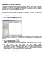
 From the Start Menu, select Start, Programs, PowerOLAP.
The PowerOLAP main application window appears:
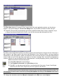
 Select File, New Database, or click on the New Database button on the toolbar. The following New
Database dialog box is displayed:
 Click Browse in the Database Name text box.
 In the Save As dialog, type QS Database in the File name text box, and follow the directory path:
C:\Program Files\PowerOLAP\Examples\.
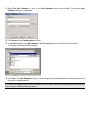
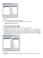
 Click Save. The New Database dialog box returns, displaying the Database Name as well as the path and
file name of the database file.
In this case the Database Name will be the same as the File Name (shown in the following figure); you have the
option to type in a different Database Name.
Notice the Secure Database and the Allow Reserved Characters checkboxes. Leave the default settings,
unchecked and checked, respectively.
The Secure Database checkbox enables you to require a password to open the database. Thus if you check the box, then click
OK, you will be prompted to give a password (and then verify it). For more information about Security, see the section in the
PowerOLAP User Manual dedicated to Security features.
The Allow Reserved Characters checkbox allows you to use so-called “reserved characters”—e.g., quote, period, comma,
etc.—in your database. See General Options further on in this manual for a list of these characters.
The Synchronization Server area of the dialog refers to a PowerOLAP component that allows PowerOLAP databases to be
synchronized via a shared file. The Synchronization Server area is activated if your license includes Synchronization Server
capabilities (see the Synchronization Server manual); otherwise, it is grayed out (as above). Consult your Administrator to
determine whether this tool is part of your application.
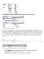
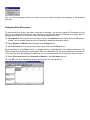
 Click OK. Note that in the PowerOLAP window, all eight menu items appear, and that several more toolbar
buttons are now active.
Notice the status area, circled in the figure. From left to right, the boxes indicate:
Whether you are working in Local or Server mode (Server name will be indicated);
The Database Name; and
Synchronization Server Name, if active.
Only one database file (“.olp”) may be open at a time. Therefore, a new database can not be created if a database is
currently open.
IMPORTANT: If you are working as a Client to an MDB Server, you cannot create a database on the Server. Typically, a
new database shared by multiple clients would be created from the MDB Server Control Program. It is worth noting,
though, that a user can create a database in standalone mode that can then be made available to the Server.
Example 2 – OLAP Dimensions and Members
Creating Dimensions
Dimensions are lists of related terms used to organize your data. Thus, a natural Dimension name
for the Members January, February and March might be Months. Dimensions, in turn, are used to
construct Cubes, the multidimensional structures in which you store and model data.
Create a
New
Dimension
In the model we are about to create, we will define three Dimensions: Months, Accounts, and
Regions.
Create the Months, Accounts, and Regions dimensions as follows:
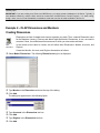
 Select Model, Dimensions. The following Dimension dialog box is displayed.
 Type Months in the Dimension text box at the top of the dialog.
 Click Add.
The dialog box appears as in the following figure:
 Type Accounts in the Dimensions text box.
 Click Add.
 Type Regions in the Dimensions text box.
 Click Add.
You can use the Enter key in place of clicking the Add button to add Dimensions to the database.
Once you have entered all of the Dimensions above, the list box will appear as in the following figure:
 Click OK. You are returned to the PowerOLAP main application window.
Adding Members to Dimensions
Create
New
Member
Dimensions are composed of Detail and Aggregate member types. Detail members “add up” to
Aggregate members. For example, in the Months dimension you would make January, February,
March (all Detail members) add up to 1st Quarter (Aggregate member).
To add Members to a Dimension:
 Select Model, Dimensions. You are returned to the Dimensions dialog box.
 Double-click on Months;
or select Months, then click Edit.
The Months dimension is currently selected for editing, as indicated in the Dimension
Hierarchy dialog title bar ('Months' Hierarchy).
Create
New
Member
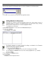
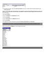
 Select the Create New Member icon;
or right-click within the Member list box (on the left in the dialog) and select New.
 Type January in the Members text box (over the currently highlighted text—e.g., Untitled3).
 Press Ctrl-Enter.
 Type February in the Members text box.
 Press Ctrl-Enter.
The Member list box will appear as follows:
 Using this procedure, enter the remaining months of the year—these will be the Detail members in the
Months dimension.
Next, you will create what will eventually be the Aggregate members for the Months dimension in the same
manner (we say “eventually” because before a Hierarchy is created, all Members appear with the Detail icon—
the number sign):
 Press Ctrl-Enter.
 Type 1st Quarter in the Members text box.
 Press Ctrl-Enter.
 Type 2nd Quarter in the Members text box.
 Press Ctrl-Enter.
 Complete the Months dimension by adding 3rd Quarter, 4th Quarter and Total Year.
You can double click on a name, or use the right mouse button, to rename or delete a name in the Member list box.
When you are done, the Member list box will appear as follows:
If the Member names are not in the order you want, click and drag them to the desired position in the list.
Example 3 – Hierarchies and Aggregate Weights
Creating a Dimension Hierarchy
Once the Members have been defined for a Dimension, the Hierarchy of these Members must also be defined.
The Hierarchy determines the aggregation of Dimension members.
You will now create the Hierarchy by selecting Members and moving them to the Hierarchy Definition dialog
box on the right side of the Dimension Hierarchy dialog box. We will proceed by creating the Hierarchy for the
Months dimension.
Define the Hierarchy for the Months dimension as follows:
 Select Total Year from the Members list box on the left.
 Drag it so that it is placed just below Months in the Hierarchy Definition box on the right, so that it
appears as below:
 Select 1st Quarter, press the Ctrl key, and holding it down, select 2nd Quarter, 3rd Quarter, and 4th
Quarter.
 Place the selection just below Total Year in the Hierarchy Definition dialog box, so that a sigma sign (for
sum),
, appears beside Total Year. This indicates that Total Year is now an Aggregate member, the
sum of the Members you placed below it (see following figure).
 Select January, hold down the Shift key, then select March in the Members list box so that February is
highlighted also.
 Drag and place the selection just below 1st Quarter in the Hierarchy Definition dialog box. Now the
sigma sign appears beside 1st Quarter.
 Pressing the Ctrl key, select April, May and June. Release the Ctrl key. Now Select 2nd Quarter in the
Hierarchy Definition dialog box.
 Press the Add Selected Members as Child button,
, on the toolbar. Notice that the sigma sign
appears, next to 2nd Quarter.
 Bring over July as a Detail member under 3rd Quarter.
 Highlight August and September from the list on the left and highlight July on the right.
 Click on the Add Selected As Sibling button,
, to add August and September into the Hierarchy
under the 3rd Quarter. Now August and September are shown under July, and the three Members
comprise 3rd Quarter.
[Note that other buttons are available for Hierarchy creation: Add all Members as Child,
Sibling button,
, and Add All As
.]
 Complete the Hierarchy for the 4th Quarter so that when you are done, the Hierarchy looks as follows:
 Close the Dimension Hierarchy dialog by clicking the OK button,
, the rightmost button on the toolbar.
You are returned to the Dimension dialog box.
Next, you will create the Hierarchy for the Accounts and Regions dimensions:
Add the following Members into the appropriate Dimensions. You will define their type, whether Detail or
Aggregate, according to the Hierarchies you see in the following two figures (next page):
When complete, the Dimension Hierarchies for Accounts and Regions should look as follows:
'Accounts' Hierarchy dialog box
'Regions' Hierarchy dialog box
A hierarchical relationships—as you completed in the three Dimensions, Months, Accounts and Regions—
defines a parent-child relationship between Members. Just as we have member siblings that exist on the same
level in a Hierarchy under an Aggregate member, we also speak in terms of Child members, which are defined
as all Members that make up parent aggregations. It is important to note that a Child member is not
necessarily a Detail member. Child members may themselves be parents of other Members within a Hierarchy.
For example, in the Regions dimension, North America is an Aggregate member; but it is also a child of Total
Regions.
The Dimension Hierarchy Toolbar
The buttons on the toolbar in the Dimension Hierarchy dialog box, and the functions they perform, are as
follows:
1. Create New Member: Add a new Member (or press Ctrl-Enter to successively add new Members).
2. Format: Select formatting option for the corresponding cells.
3. Member Aliases: Define and edit Aliases and Alias Groups for the selected Member.
4. Alias Group: Add or delete Alias Groups, and assign names for each Member.
5. Properties: Assign Members a property for annotation purposes. A Member’s properties can be displayed on an
Excel worksheet when needed.
6. Mark Member as Persistent: Tag a Member as ‘persistent’ to prevent its data from being overwritten when
updates or Cube re-builds occur.
7. Add Selected as Sibling: Insert the selection in the Member list on the left into the Hierarchy Definition on the
right, below the selected Member.
8. Add All as Sibling: Insert all Members in the Member list after the selected Member in the Hierarchy, making
them sibling Members.
9. Add Selected Members as Child: Insert selected Member(s) in the Member list as children of selected Member
in the Hierarchy.
10. Add All Members as Child: Insert all Members in the Member list as children of selected Member in the
Hierarchy.
11. Specify Member Weights: Edit the weight of a child Member (active only when a child Member is selected in the
right hand Hierarchy Definition box).
12. Help: Accesses the help screen for the Dimension Hierarchy.
13. OK: Exits the dialog, with changes made and saved for the Dimension.
The functions listed above are described more fully in the PowerOLAP User Manual, though we will now
discuss Aggregate weights in order to complete our QS Database Dimension set-up.
Aggregate Weights
Specify
Member
Weight
Aggregate weights are used when a Member must be assigned a multiplied value in an
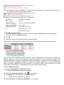
aggregation in order for the data to be properly represented. For example, in the Accounts
hierarchy, Cost of Sales should be handled as a negative number in the Gross Profit aggregation
because it will represent an amount subtracted from Gross Profit (i.e., Gross Profit = Net Sales Cost of Sales). To designate Cost of Sales as a negative number in the Gross Profit aggregation,
we can assign it a weight of “–1”. This means that the data included in Cost of Sales will always be
multiplied by –1 when it is rolled up in the Hierarchy.
To “weight” Cost of Sales, complete the following process:
 Return to 'Accounts' Hierarchy dialog box (double-click on Accounts in the Dimensions dialog), and
double-click Cost of Sales in the Hierarchy Definition box on the right. Note that, to the right of Cost of
Sales, a box appears where “1” is highlighted and where you can enter a weight for the Member.
 Enter -1 in the box so that it appears as follows:
 Click the OK button,
, on the toolbar when complete.
You are returned to the Dimension dialog box.
 Click OK. You are returned to the main application window.
In PowerOLAP, the default Aggregate weight is equal to ‘1’. Thus, a parent Aggregate member is simply the sum of all
Child members defined in the Dimension hierarchy. In the example exercise, all Aggregates you defined are standard with
the exception of Gross Profit, in the Accounts dimension. Therefore, you do not need to define Aggregate weights for the
remaining Aggregate members.
Example 4 – OLAP Cubes and Slices
Creating a Cube
Cubes
Using the Dimensions created in the previous exercises you will now create a PowerOLAP Cube
that will store and model your data.
To create a Current Year Budget cube:
 From the main application window, select Model, Cubes.
The Cubes dialog box is displayed:
 Type Current Year Budget in the Cubes dialog box.
 Click Add.
The Define Cube dialog box appears, in which you select Dimensions to be used by the Cube:
 Select all of the Dimensions in the Available Dimensions list box by clicking the
button.
All three Dimensions are moved to the Selected Dimensions list box on the right.
 Click OK. Note that the Current Year Budget cube is now listed in the Cubes dialog box.
All of the Cubes dialog’s buttons on the right are activated. These buttons control functionality associated with
Formulas and setting Security privileges, as well as the OLAP Exchange capability to push data ranges back to a
relational database—they are covered in depth in the PowerOLAP User Manual and OLAP Exchange manual
respectively.
 Click OK to return to the main application window.
The Current Year Budget cube is now ready for data input.
Creating a Slice View
PowerOLAP provides a method for looking into a Cube to view and input data. This means of
viewing and inputting data is known as “creating a Slice.” A Slice is a two-dimensional view of a
Cube that arranges data in a grid, just as a spreadsheet does. You can create Slices “on the fly”
New Slice
to see any view of a Cube, or you can save and re-open Slices for ongoing data viewing or
inputting. Finally, as you will see, you can instantaneously create an Excel spreadsheet from
any Slice view.
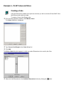
To create a Slice called Regions by Account:
 Select Slice, New. The following New Slice dialog box is opened. The list box displays the names of
available Cubes in your database. In our case, we just created the only Cube listed, Current Year Budget.
 With the Current Year Budget cube selected, click OK.
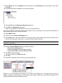
The Slice View dialog box is opened in the Content Area of the main application window, as in the above
diagram. The window displays a Current Year Budget slice, as yet untitled, and with no data in the grid.
 Press F9. (This manually recalculates the grid’s data, explained further below.) Keep in mind that, as yet,
no figures have been entered into the Cube, so you will see zeros as data throughout the Slice.
By default, when PowerOLAP creates a new Slice, it places the last Dimension brought into the Cube when it
was created in the Rows position, the next-to-last Dimension in the Columns position, and any remaining
Dimension(s) in the Page position. (When we created the Cube in the last exercise, we brought all Dimensions
into the Cube at once in the order they were listed.) In the above example Slice, Accounts are displayed as
columns, Regions as rows and Months as the Page dimension, currently displaying January, which is the first
Member entered for the Months dimension.
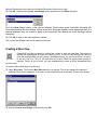
 Select Slice, Save As to save the Slice.
 Type Regions by Accounts in the Slice Name text box.
Save
Slice
 Click OK. You are returned to the Slice—note that both the Cube name, Current Year Budget,
followed by the Slice name, Regions by Accounts, appear in the title bar.
NOTE: PowerOLAP’s default calculation mode is set to Manual. Thus, when you make changes to a Slice, you
will need to Press F9 (or the calculator button on the menu bar) to see those changes reflected in the Slice. You
can change the calculation mode to Automatic by selecting Edit, Options, and clicking on the Automatic radio button in
the General tab.
 Change the calculation mode from Manual to Automatic on the Edit menu under Options.
Now you will see changes instantly on screen as they are made throughout the remainder of this manual’s
exercises.
Arranging Slice Dimensions
To demonstrate how quickly and easily views can be changed, you will now arrange the Dimensions of this
Slice to view data with Accounts as rows, Months as columns and Regions displayed as a page. Start by
dragging and dropping the Dimension names into the appropriate list boxes:
 Select Months in the Page list box and drag it down to the Columns list box, below Accounts. [Note that a
“nested” view is created, assuming you are operating in Automatic calculation mode.]
 Select Regions in the Rows list box and drag it up to the Page list box.
 Select Accounts in the Columns list box and drag it down into the Rows list box.
By placing Regions in the Page list box, you display data for a single Member of the Regions dimension. The
Page member you see when you first arrange a Slice is the Member at the top of that Dimension’s member list.
In this case, the Slice grid displays the data for all Accounts and all Months for the Regions member Canada.
 Select Slice, Save As and type Accounts by Months in the Slice Name text box.
 Click OK. You have created and saved a second Slice, Accounts by Month:
Selecting Page Members
Set
Page
Member
Currently you are viewing data for Canada. To view data for other Members defined in the Regions
dimension within the Accounts by Months slice—e.g., to change the view from Canada to United
States:
 Double click on Regions: Canada in the Page list box.
The following Edit Slice dialog box is displayed (in this example, Edit ‘Regions’ for ‘Accounts by Months’):
Note that the Detail member icon to the left of Canada in the Slice Content list box is yellow, indicating that
this Member is the currently selected Page member.
You can select any Member in this list box as the Page member to view within the Slice:
 Double-click United States in the Slice Content list.
The icon beside it is now yellow. You may also select a Page member by clicking on the Select Page
Member icon,
, from the menu bar.
 Click the OK button,
, on the toolbar, to close the dialog and return to the Accounts by Months slice.
The current Slice now displays data for United States, which is indicated in the Page list box, beside Regions
(i.e., Regions: United States).
Changing the Grid Layout
You can change the layout of the Slice grid by moving Members of a Dimension within the Slice Content list
box:
 Double-click on the Months dimension in the Columns list box in your current Slice. The Edit Slice dialog
box is displayed.
Currently, Total Year is at the bottom of the Slice Content list box, which corresponds to the rightmost column in
the grid (you may need to scroll rightward in the grid to see Total Year). By dragging and dropping Total Year to
the top of the list, you can move it to the leftmost column:
 Select Total Year from the Slice Content list box on the right.
 Drag and drop Total Year above January, as circled below.
 Click the OK button,
, on the toolbar.
You are returned to the Accounts by Months slice, and Total Year is now displayed in the first column of the
Slice.
Entering Data in a Slice
So far, you have demonstrated PowerOLAP’s remarkable flexibility in organizing and displaying data within a
Slice. Next, you will demonstrate another key function of the Slice: using a Slice to enter data directly into the
underlying PowerOLAP database.
Currently, the data in the Current Year Budget cube is all zeros because it is a new Cube and data has not yet
been entered into it.
To enter data into the Accounts by Months slice:
 Click the cursor at the intersection of January and Net Sales.
Type 5000, then press Enter.
 Click the cursor at the intersection of January and Cost of Sales, Type 3000, then press Enter.
Notice that PowerOLAP has automatically adjusted the values in data cells that occur at the intersection of
Aggregate members, reflecting the values entered above.
 Try to type 100000 at the intersection of Total Year and Gross Profit.
PowerOLAP does not allow you to change the values in data cells involving one or more Aggregate members.
PowerOLAP will automatically update these cells only when the values in relevant Detail members change.
Settings General & Format Preferences
Before continuing to work with data in a Slice, we will take a look at some preferences, among which are those
that affect the look of a Slice.
General Tab
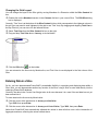
Selecting the Options command from the Edit menu enables you to set several general database options.
 Select Edit, Options. The Options dialog box is opened, with the General tab on current settings.
Calculation Mode
As discussed previously, the radio buttons will allow you to show Slice changes and data entry calculations
upon entry (Automatic) or upon pressing F9—similar to your experience with Excel.
Example 5 – OLAP Cube Formulas
You have seen how creating Dimension hierarchies, and assigning Aggregate weights, results in the natural
“summing up” of values. Cube formulas represent a powerful extension of your ability to perform mathematical
calculations throughout a PowerOLAP database. With Cube formulas, you can perform all manner of calculations
to populate a cell, ranges of cells, even entirely different Cubes.
Presently your Current Year Budget cube contains data for January for all Accounts and Regions. The
following Cube formula will populate the month February.
 Select Model, Cube. The Cube dialog box is opened
 Click on the Current Year Budget cube to select it.
 Click on the Formulas button. The Formulas dialog box is opened:
We will now make use of some buttons in the Formula dialog box (also known as the Formula Editor). These
buttons will enable us to specify the area of the cube we want to populate with data, and where the data will
come from.
 Click on the “squiggly brackets”—
.
The Build Range Reference dialog appears.
Months is selected in this dialog at the top of the Dimension list; it is the Dimension we want to work with,
so leave as is.
 For
the
Qualifier
(top
left),
select
the
radio
button
This indicates that only Detail members are to be calculated by the Cube formula—Aggregate
will be calculated according to the Dimension hierarchy. (Note: it is possible to “overwrite”
calculations via a Cube formula, a very important feature if you wish to calculate a “what if” or
Aggregate data point, so that it contrasts to actual figures in Detail data points.)
 On the right, select February among the Months.
(The Selected radio button is selected, as a consequence.)
The dialog appears as follows, with the formula as it exists so far, at the bottom:
Details.
members
hierarchy
budgeted
 Click OK.
 Click on the “equals” sign in the Formula Editor,
.
The left-hand side of the formula is completed, and is shown in the content area.
 Next click on the “square” brackets —
.
The Build Cube Reference dialog box appears.
Again, Months is selected; it is the Dimension we want to work with, so leave as is.
 Select January from the Member list on the right. (The Selected radio button is selected, as a
consequence.) [Note that at the top of the dialog, there is a Cubes drop-down.]
This brings up an important feature—the ability to create cross-cube formulas, which is explained in the
PowerOLAP User Manual. There is only one Cube in our database, Current Year Budget, in the formula
we are creating, data will come from this Cube, to populate another area of the same Cube.] The Build
Cube Reference dialog box appears as follows:
 Click OK.
The Formula Editor content area appears as follows (you can hit Enter after the “=” to show the formula on
two lines)”
 Use the buttons in the Formula Editor — the asterisk (for multiplication), the numbers and the semi-colon
— to complete the formula to that it appears like so:
Following is a breakdown of the syntax of the Cube formula:
Left of equal ‘=’
Area of cube to populate
Right of equal ‘=’
Formula
{"Months.February"}
Dimension and Member to populate
"Current Year Budget"
Source cube
["Months.January"]
Range within source cube
1.5
Value (in this case, +50%)
;
Ends formula statement
 Click OK to save the formula.
(If you have mistyped the formula, you will receive a message indicating that there is syntax problem.)
You are returned to the Cubes dialog box.
 Click OK.
 Press F9 in the Accounts by Month slice to recalculate values.
Notice that the February column has been populated by the Cube formula defined in the previous steps.
Next, you will create a Cube formula that calculates a ratio of two Members. You will first need to add a new
Member—Margin %—to the Accounts dimension, and then modify the Accounts dimension hierarchy. This
Cube formula exercise brings up two important strengths of PowerOLAP, in comparison to static modeling tools,
OLAP or otherwise: the capability to create new, “on-the-fly” calculations (which can of course be subsequently
saved) for precisely specified (even new) components of a business model, which themselves are created
entirely within PowerOLAP [i.e., not dependent on any static model of business data].
 Select Model, Dimension.
 Double click Accounts in the Dimension list box.
The 'Accounts' Hierarchy dialog box is displayed.
 Click on the Create New Member button,
, on the toolbar.
 Type Margin % so that it appears in the Members list box.
To modify the Accounts dimension hierarchy:
 Expand Accounts in the Hierarchy Definition box, on the right.
 Select Margin % from the Members list box and drag it to the Hierarchy list box and release it just under
Accounts.
The completed hierarchy will appear as in the following figure:
 Click the OK close the Dimension Hierarchy dialog box.
 Click OK in the Dimensions dialog box.
Margin % now appears as the top row in the Accounts by Month slice.
Next, you will define a Cube formula that creates values for the new Margin %: the values will be based on a
formula that divides Gross Profit by Net Sales:
 Select Model, Cube.
 Double-click the Current Year Budget cube.
 Press Enter twice in the Content Area to move the previously written formula down two lines. Begin on the
top line of the Formula Content area, i.e., place this formula above the other.
Priority, which is top-to-bottom in the Formula editor, is very important for determining data calculations—consult the
PowerOLAP User Manual.
 Using the Formula Editor dialog box, create the formula:
All and {"Accounts.Margin %"}=
"Current Year Budget".["Accounts.Gross Profit"]/
"Current Year Budget".["Accounts.Net Sales"]*100;
 Click OK to save the formula.
You are returned to the Cubes dialog box.
 Click OK.
 Press F9 to recalculate values in the Accounts by Month slice.
Margin % is now calculated for all Months in the Current Year Budget cube. The figure above shows the
Margin % figures for United States. You can select other Regions members to verify that all members in the
Regions dimension have been updated as well.
 Select File, Save All to save the data and the Slice (which now includes Margin %) to disk.
Example 6 – OLAP and Excel
Creating an Excel Worksheet
Create
Excel
Worksheet
One of PowerOLAP’s key features is that it enables you to create an Excel worksheet from a
PowerOLAP slice. You can then work with data in Excel, utilizing all that product’s features and
functions while maintaining a dynamic connection to the PowerOLAP database. This is why
PowerOLAP is credited with having a “spreadsheet front end.”
To create an Excel worksheet from the Accounts by Months slice:
 Select Slice, Worksheet; or press F8; or click on the create worksheet button,
, from the menu bar.
PowerOLAP launches Excel (assuming it is not running), displaying the newly created worksheet. A new Excel
worksheet appears, as follows:
The first few rows of the worksheet display information indicating the PowerOLAP database; the Cube; the Page
Dimension member(s) that the Slice data shows (in the figure above, one Page Dimension, Regions, and United
States is shown); and the Dimensions “Along Rows” and “Along Columns”.
The worksheet can now be saved as an XLS file via Excel’s Save command.
Selecting a Page Member to View in Excel
Change the Page member in Excel as follows:
 Double-click Page member cell—e.g., cell C3 (United States).
The Select a Member dialog box appears. Note the two tabs (circled): you can find Members based on where
they appear in the dimensional hierarchy or in the Member list (this tab is selected below).
 Select Canada.
 Click OK, and then press F9 to update the worksheet.
The worksheet now shows data for the new Page Member, Canada. You can repeat this means of selection—
via the Select a Member dialog, which PowerOLAP has made available in Excel—to pick other countries in
the Regions dimension. [Were this a four-, five- , etc. dimensional Cube, you could pick any number of Page
members to view, multiplying your potential sheaf of reports manyfold!]
Entering Data from within Excel
You can enter data into a PowerOLAP database using an Excel worksheet. This has great applicability in
forecasting, planning and budgeting systems that use PowerOLAP. All data entered into a worksheet is
automatically updated using one of PowerOLAP’s functions (OLAPTable has been shown here), each of which
maintains a “bi-directional, dynamic spreadsheet connection” between PowerOLAP and Excel.
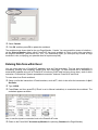
To enter data via an Excel worksheet:
 Select a cell at the intersection of Detail members, such as F7, which is the cell at the intersection of April,
Net Sales.
 Type 100000.
 Press Enter, and then press F9 (if Excel is set to Manual calculation) to recalculate the worksheet. The
worksheet appears as below:
Now, to see the dynamic connection back to the PowerOLAP cube:
 Return to the PowerOLAP Accounts by Months slice (showing Canada as the Page Member).
 Press F9 to update PowerOLAP.
The Slice appears as follows:
The data you entered in the Excel worksheet is now reflected in the PowerOLAP database. Because
PowerOLAP’s function connecting to the worksheet (OLAPTable, in this case) is bi-directional, you can enter
data in either Excel or PowerOLAP and select F9 to update. (Note you can not write into Aggregate member
spreadsheet cells or cells governed by a Cube formula, just as in a Slice).
The strength and power of the spreadsheet connection to PowerOLAP cubes are central to the use of the product:
PowerOLAP “disburdens” Excel of its calculation tasks—hierarchies/ Aggregate weights/formulas are calculated in
PowerOLAP’s engine, across specifiable multidimensional data ranges; further, PowerOLAP relieves users/organizations
of the difficulties of maintaining hundreds or more linked spreadsheets.
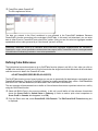
Defining Cube References
The bi-directional connection shown so far is OLAPTable function (shown in cell A6). In fact, when you click on
cell A6 in the worksheet, you will see in Excel’s formula bar the single formula that references all the worksheet
cells that connect to data in the PowerOLAP cube:
=OLAPTable($B$1,$B$2,B5:R5,A6:A9,$C$3)
The OLAPTable function is one of many functions you can use to dynamically link data between a worksheet and a
PowerOLAP database. (The other PowerOLAP functions for creating a worksheet from a Slice—OLAPReadWrite
and OLAPPivot—and their differences, are discussed in the PowerOLAP User Manual.)
The next exercise will demonstrate how to define a Cube reference that returns a pertinent value into a cell by
using the OLAPRead function.
 Select cell D13 in Excel in the current worksheet. In this cell, you will define a Cube reference formula that
shows the Gross Profit for United States in February (in order to make a quick visual comparison to
Gross Profit for Canada, which appears in cell D9).
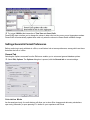
 From the Excel menu bar, select PowerOLAP, Edit Formula. The Edit PowerOLAP Formula dialog box
is displayed:
 Select OLAPRead from the top drop-down menu (to the right of Function).
 Press the Pick button,
(next to Database).
The Select Database dialog box is displayed, as below:
The current database—which contains the value you want—is selected.
 Click OK. You are returned to the Edit PowerOLAP Formula dialog box.
 Press the Pick button,
(to the right of Cube). The Select Cube dialog box is displayed. Likewise,
this Cube contains the value you want to be reference into the Excel cell, D13.
 Click OK.
Again, you are returned to the Edit PowerOLAP Formula dialog box. Now you have defined several of
the parameters of the Cube reference formula, as shown in this detail of the dialog box:
Note that the Dimensions area now displays text boxes for you to enter choices for the Months, Accounts and
Regions dimensions. In fact, February has been “pre-selected” for you. If you wanted another Months member
for your formula, you would press the Pick button to make a different selection. Since you do want to select
February data, continue to the Accounts and Regions dimensions. Use the Pick button and the corresponding
Select A Member dialog boxes to choose data for Gross Profit and United States, respectively.
After you have made these choices, the Edit PowerOLAP Formula dialog box will look as follows:
 Click OK to update Excel with the new formula reference.
Your dynamically connected Excel spreadsheet will appear as in the following figure:
You can save the current database, with changes you have made, from within Excel:
 Select PowerOLAP, Save Current Database in Modeler.
The PowerOLAP database is saved but not closed.
You now have a ready view of the February, Gross Profit for United States within a dynamically connected
spreadsheet that shows figures for Canada. Now, whenever February, Gross Profit for United States (or for
that matter, Canada) changes, it will be reflected in this worksheet.
You can save the current database, with changes you have made, from within Excel:
 Select PowerOLAP, Save Current Database in Modeler.
The PowerOLAP database is saved but not closed.
Closing a Database
The Close Database command located on the File menu in PowerOLAP closes an open database. When you
have completed work within one database, you may still wish to work with another database. You must first
close the currently open database before opening another database.
To close an open database:
 Select File, Close Database.
If any Slices are open, PowerOLAP will prompt you to save Slices.
 Clicking
Yes will save all database changes to disk and close the database file.
Clicking No will close the database file without saving any changes made to the database.
In either case, all open Slices will be closed along with the database.
As noted earlier, you can save and close any dynamically connected worksheet as a normal XLS file. Upon opening such a
worksheet, when you press F9, PowerOLAP launches, and a spreadsheet system with OLAP cubes behind it, is ready for
online, optimized planning / analysis / reporting.
Summary of Quick Start Exercises
In the preceding examples you very quickly learned important basic concepts and fundamental functions of
PowerOLAP, including:
•
•
•
•
•
•
•
•
•
Creating a PowerOLAP database, the first step in building a Cube to model multidimensional data.
Creating Dimensions, adding Members to those Dimensions, establishing a Hierarchy among Members
(whether Detail or Aggregate), and assigning an Aggregate Weight to a Child member.
Creating a Cube from Dimensions and their respective Members.
Creating a Slice, arranging Slice dimensions, selecting Page members to view, and changing the layout of the
grid within a Slice.
Setting general and formatting preferences from the Edit, Options Menu.
Entering data in a Slice, and seeing how PowerOLAP automatically recalculates Aggregate members to reflect
changes in value. Then, saving those changes to a database.
Creating Cube formulas.
Creating a fully functional Excel worksheet from a Slice, and defining database reference formulas.
Saving changes made from within Excel into the PowerOLAP modeler, and closing the PowerOLAP database,
knowing that you can reopen it from a normal Excel worksheet.
Now that you have grasped the concepts and demonstrated these many functions, you are well prepared to
use PowerOLAP in a production environment. For more detailed instruction on using PowerOLAP, and to learn
additional features, see the PowerOLAP User Manual or email us at [email protected].