Download pdf-document

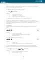
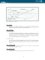
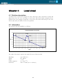
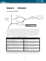
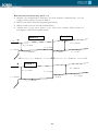
SOBEK-RE exercises
Handout
SOBEK
February 2007
1
Chapter 1
Introduction
1.1 Introduction
This is the user manual for the exercises of the River Systems & River Dynamics (Module
5) course at the Unesco-IHE. The main goal of these exercises is to get experience with
morphological modelling. The one-dimensional SOBEK-RE modelling system is used for
this exercise. This system has been developed by WL | Delft Hydraulics and
Rijkswaterstaat RIZA, and is used for understanding and predicting river behaviour. More
information can be found at www.sobek.nl.
Note: this exercise has been designed and applied at the Delft University of Technology,
part of the course CT5311 on River Dynamics.
1.2 Contents
Chapter 2 gives a short introduction into SOBEK-RE. The set-up of a new model is
discussed in Chapter 3. This knowledge is needed for both exercises. The two exercises are
presented in Chapters 4 and 5 respectively. The first one, 'Local shoal', can be considered
as a basic introduction to the modelling system and the type of morphological processes
that are reproduced. You have to do all 'model steps': bathymetry, boundaries, runs,
interpretation of the results, etc. The second exercise 'Bifurcation' is more complex. The
schematisation of this exercise will be made available to you. You have to analyse the
effects of management strategies on the morphological behaviour of the river.
1.3 Information
For questions please contact:
dr. ir. Kees Sloff (WL | Delft Hydraulics, phone 015-2858585, [email protected])
2
Chapter 2
Description of SOBEK
2.1 Introduction
SOBEK is a one-dimensional modelling system for open-channel networks. It can be used
to simulate unsteady and steady flow, (uniform and graded) sediment transport,
morphology, salt intrusion, and water quality. SOBEK is developed by WL DELFT
HYDRAULICS and Rijkswaterstaat RIZA (Rijksinstituut voor Zoetwaterbeheer en
Afvalwaterbehandeling), in The Netherlands. Presently there are two versions for river
applications:
SOBEK-RE: the original version to be used for this SOBEK Exercise, in which “RE”
refers to Rivers and Estuaries. This version was developed in the period between 1995
and 2000, and remained unaltered since then. SOBEK-RE is still used for the
morphological model, but will be replaced in the future by SOBEK-RIVER.
Figure 1 Graphical User Interface of SOBEK-RE
SOBEK-RIVER is the new version of SOBEK, capable of simulating 1D channel flow
and 2D flooding. It is part of the new product line of SOBEK, which integrates all
modules in a GIS environment. Although it is more user-friendly and more flexible
than the SOBEK-RE, it does not yet contain an ‘easy to use’ morphological module.
Therefore SOBEK-RE is chosen as tool for this exercise.
3
Figure 2 Graphical User Interface of SOBEK-RIVER (GIS based)
2.2 Hardware
Sobek can be used on a PC with MS-Windows. For normal applications SOBEK needs at
least a Pentium II processor or higher. The PC version can only be used with a hardware
key. Unauthorized use is not possible.
2.3 Equations
Water motion
In Sobek the one-dimensional mass balance and momentum balance for water motion are
solved. Without wind and density differences, these equations read:
At
t
Q
t
Q
x
x
in which:
Q
t
x
B
Af
At
g
h
(1)
0
Q2
B
Af
gAf
h
x
gQ Q
C 2 RA f
(2)
0
= discharge [m3/s]
= time [s]
= distance [m]
= Boussinesq coefficient [-]
= cross section with flow [m2]
= total cross section [m2]
= acceleration due to gravity [m/s2]
= water level [m]
4
C
R
W
= Chézy coefficient [m1/2/s]
= hydraulic radius [m]
= flow width [m]
Note that in a situation with steady-uniform flow the water depth approaches the normal
depth value. The normal depth follows from equation (2) by eliminating the accelaration
and convection terms, and replacing the surface slope h x by the bed slope i [m/m]:
hn
Q2
W 2C 2i
3
The flow velocity u then follows from the continuity equation: Q=Wuhn
Sediment transport
A sediment transport formula can be selected, for instance Engelund-Hansen or MeyerPeter-Müller. Often sediment transport formulas can be rewritten as a power law of the
flow velocity:
s
aub
(3)
in which
s
a
b
u
= sediment transport per unit width, excluding pores [m2/s]
= coefficient [m2-b/s1-b]
= exponent representing the degree of nonlinearity [-]
= current velocity [m/s]
In transport formulas in SOBEK the Shields parameter is often the governing parameter. It
is defined as:
u2
C
2
D
in which:
D
h i
D
= characteristic grain size of bed material [m]
= relative density of sediment (for sand = 1.65) [-]
= Shields parameter [-]
The formula of Engelund and Hansen can be written (for transport without pores) as:
s
0.05 g D503
in which:
u*
D50
C2
g
5/ 2
0.05
u5
gC 3
2
D50
= shear velocity = (u· g)/C [m/s]
= median grain size of bed material [m]
5
Engelund and Hansen is valid for situations in which ws/u* < 1, 0.19 < D50 < 0.93 mm, and
0.07 < < 6 (in which ws is the fall velocity)
The formula of Meyer-Peter and Müller is defined as:
s = 8 Dm3/ 2 g
in which:
Dm
0.047
3/ 2
= mean grain size of bed [m]
= ripple factor = (C/C90)3/2 [-]
= grain roughness = 18·log(12h/D90)
C90
It is valid for situations in which ws/u* > 1, Dm > 0.4 mm, and
< 0.2.
To obtain the sediment-transport rate including pores, it is necessary to multiply the
equations above with a factor 1/(1- p) in which p is the porosity of the bed (in the order of
0.4). Output of sediment-transport rates from SOBEK-RE is presented as transport
including pores.
Bed level
For the bed level, the sediment transport balance in SOBEK is used for the total cross
section:
1
1
p
A
t
S
x
in which:
A
S
(4)
0
= area of cross section [m2]
= sediment transport through a cross section [m3/s]
= fraction of pores [-]
p
For a constant width, this equation reduces to:
1
1
p
zb
t
in which:
zb
s
s
x
(5)
0
= bed level [m]
= sediment transport per unit width, excluding pores [m2/s]
For these balance equations de Vries (1965) has shown that small-scale disturbances
propagate in flow direction with a speed cb following from the method of characteristics:
cb
um
in which
b
Fr
1 Fr 2 where
ds / du
h
b
S
and cb in [m/s]
Q
= power of transport formula (see equation 3)
= Froude number = u (gh)
6
Chapter 3
Model set-up
3.1 Starting SOBEK
Sobek has been installed on the network. Start the SOBEK software and open a new
project and save this project directly with a new name, e.g. "ex1". Then, open the 'empty
case' and save this case with a new name, e.g. "ex1". You see three yellow boxes at the lefthand side: Model schematisation, Hydraulic computation, Hydraulic results. These boxes
can be entered by clicking on them. Each box is discussed separately in the next
subsections. The other boxes on the screen are not used during these exercises.
3.2 Model schematisation
3.2.1
Model attributes
When building a new model, go first to 'Model Attributes' under 'File'. On this screen, parts
of SOBEK can be activitated for the current case.
For case 'Local shoal'
'River', 'Water Flow', 'Sediment Transport' and 'Morphology'.
Besides, the geographical area must be specified in this window. Choose a sufficiently large
area for your model.
Specify the 'Geographical Area' of the river in X and Y coordinates
Then, the model schematisation itself should be specified in the Select Layer window at the
right hand side. The following parts are important for this exercise:
3.2.2
Nodes, branches and cross-sections
Mind the difference between nodes, branches and cross sections:
A node is only used for an internal bifurcation or confluence or an external
boundary. These nodes are defined in the horizontal plane and only have an xand y-coordinate.
Between two nodes, a branch is defined. It represents the actual river channel
between bifurcations, confluences or boundaries. Many models consist of one
branch only!
Cross sections are defined to prescribe the (varying) bed levels and widths of the
cross-sectional profile along a branch or river.
7
<Topography>: Defining nodes and branches: with these nodes and the branches, the
topography in the horizontal plane is defined (see Figure 3).
Nodes:
Specify the nodes of the river by giving a name and the coordinates in X
and Y.
Branches:
Specify the branches of the river by giving a begin and end node
Branch 1
Node 1
(x1,y1)
Figure 3
Node 2
(x2,y2)
Definitions of nodes and branches
Thereafter, the cross section must be defined. The definition is split into two parts:
<Definitions>: cross section shape (width versus distance from the lowest point in the
cross section)
Define the cross-section of the river. Start with the 'level width table' by
clicking on 'tabulated' (see Figure 2).
<CrossSections>: cross section location (and height)
Define the location and the reference level of the cross section. Determine first
how many locations must be given and if you would use a slope (“slope” is only
necessary if SOBEK cannot determine the slope from interpolation between two
cross-sections on a branch). The reference level is used to determine the height of a
cross-section relative to a reference level (only if the height had not been set yet
relative to this reference in ‘descriptions’).
Each river branch must have at least one cross-section at a certain distance from
the begin node with a specified height. More than one cross-section should be
defined in a river branch if the cross-sections are not uniform or if the slope is not
uniform (see figure 4).
8
Figure 4 Definition of cross-sections
3.2.3
Friction
Define the roughness predictor. Give values for 'flow' and 'reverse flow'.
Although the river flow in a situation without tidal influence has always the same
direction, the roughness must be given for both directions.
3.2.4
Conditions
Boundary conditions:
Specify the boundary conditions for ‘water flow’ and ‘morphology’. You can
also specify lateral discharges, dredging etc. Although a river without tidal influence
only needs a condition for the bed level or the sediment transport at the inflow
boundary, SOBEK also requires a boundary condition at the outflow boundaries.
Set the sediment transport rate at this boundary at zero.
Initial Conditions:
Specify initial conditions and grain sizes. Note that if a sediment transport
formula is selected (see later), SOBEK will only ask for the grain size required by
that particular formula. Otherwise all grain sizes (D35, D50, Dm and D90) are
required.
3.2.5
Numerical grid
To generate a grid with constant mesh size, it is necessary to specify the grid
size ('distance') and generate a grid.
3.2.6
Run time data
Time Parameters:
Specify the begin and end time (note the format!) and the time step.
9
Numerical Parameters:
Change the calculation mode into ‘Steady’ (for quasi-steady simulations).
F(x), F(t) reports:
Specify the parameters and time steps for your output. If you change the
simulation time or computational time step, you should probably also change the
output time step etc.! The output ‘time step’ indicates the number of computational
time steps after which output is written to file (and is therefore not expressed in a
time unit, such as hours).
3.2.7
Transport formula
Choose a sediment transport formula which is suitable for your problem.
3.2.8
Validation
Once all the input has been specified, the model input can be validated by using
'Operations' and 'Validate model'. If all data are correct, you can leave the 'Model
schematisation' and go to 'Hydraulic computation'.
3.3 Hydraulic computation
Start the simulation in the box 'Hydraulic computation'. When an error occurs, go back to
'Model schematisation' to check your input. When the computation does not give error
messages, go to 'Hydraulic Results' to interpret the numerical results.
3.4 Hydraulic results
The results of the computations can be visualized by clicking the box 'Hydraulic results'.
First, select an output file, e.g. the flow output or the morphology output. Then, make
graphs of the most important variables, e.g. the bed level development and the current
velocity. The parameters can be plotted in time as well as space. The graphs can be printed
or copied to other applications.
10
Chapter 4
Local shoal
4.1 Problem description
An alluvial river section has a length of 10 km. After heavy rains, sand from a nearby hill
slides down into the river and forms a local shoal. This shoal makes navigation more
difficult. The river manager would like to know how this shoal will develop in the near
future. (S)he asks your advice for this river problem.
4.2 Information
The situation after the landslide is as follows:
longitudinal bed level profile
1.2
0.95
1.00
1
0.90
z (m)
0.8
0.6
0.45
0.60
0.4
0.2
0.00
0
0
1
2
3
4
5
6
7
8
9
10
x (km)
The sand of the shoal is equal to the sand of the rest of the river bed.
Discharge
Width
Slope
Chézy roughness
Grain size
: Q = 1000 m3/s
: B = 200 m
: i = 10-4
: C = 50 m1/2/s
: D50 = 0.2 mm (ws50 = 0.04 m/s)
11
11
4.3 Analytical exercises
Calculate the (equilbrium) water depth and the flow velocity in the undisturbed river
section.
Choose a transport formula (Engelund-Hansen of Meyer-Peter-Müller), and give a
motivation.
Calculate the annual sediment load, s (m2/s)
Compute the propagation velocity of a bed disturbance
Choose the spatial step, x
Choose the time step, t
Choose the simulation period
Information in the the book Principles of River Engineering (Jansen et al, 1979).
4.4 Simulations with SOBEK
Simulate the problem with the SOBEK-software
4.5 Exercises
How many equations does SOBEK solve dynamically?
Which model variables are computed dynamically in SOBEK?
Which initial and boundary conditions are needed for your simulation?
Draw the propagation velocity of the top of the shoal as a function of time. Is the
numerical propagation velocity equal to the analytical propagation velocity? Why?
Does the shape of the shoal change in time? Why?
Simulate the same problem for median grain sizes of 0.4 mm and 0.1 mm (twice and
half the reference value). Use the same transport formula! What is the sensitivity of the
propagation velocity of the shoal when you increase or decrease the median grain size?
Can you explain this by using the transport formula?
12
Chapter 5
Bifurcation
5.1 Problem definition
River discharge
Branch 2
Lake with
constant
water level
Branch 1
Branch 3
Optional side channel
Nevengeul
A river splits into two branches before debouching into a lake with a constant water level.
In this river system, two types of measures are being considered. The first type regards four
options of dredging to improve navigation, either by one-time deepening (options B1 and
B2) or by continuous sediment withdrawal (options B3 and B4). The second type of
measures regards four options of side channels for purposes of nature rehabilitation. It is
assumed that the side channels convey only water and do not extract any sediment from
the main river. All options of dredging and side channels are summarized in Table 1.
Table 1
Options of dredging and side channels
Dredging
Side channel
D1, one-time deepening in upper Branch 2:
S1, 100 m3/s discharge from Branch 2:
1 m lowering of bed level over reach between reach between 10 and 20 km from
0 and 25 km from bifurcation
bifurcation
D2, one-time deepening in lower Branch 2:
S2, 150 m3/s discharge from Branch 2:
1 m lowering of bed level over reach between reach between 20 and 30 km from
25 and 50 km from bifurcation
bifurcation
D3, continuous sediment withdrawal from upper
S3, 200 m3/s discharge from Branch 3:
Branch 3:
reach between 5 and 15 km from
3
0.001 m /s at 5 km from bifurcation
bifurcation
D4, Continuous sediment withdrawal from middle
S4, 100 m3/s discharge from Branch 3:
part of Branch 3:
reach between 15 and 25 km from
0.001 m3/s at 15 km from bifurcation
bifurcation
As a river engineer, you are asked to advise about the short-term effects of these measures
(first weeks after implementation) as well as the long-term morphological effects (50 year).
13
You only need to analyse one combination of a dredging option (D) and a side
channel option (S). Please select two options from Table 1.
5.2 Data
The model is already available at your computer. The input has been based on the data and
calculations below:
Data
B1 = 300 m
L1 = 50 km
i1 = 1*10-4
C1 = 50 m1/2/s
B2 = 150 m
L2 = 50 km
C2 = 50 m1/2/s
B3 = 100 m
L3 = 50 km
C3 = 50 m1/2/s
At the upstream boundary the discharge is constant and equal to 2500 m3/s. The median
grain size is equal to 0.3 mm for the entire area.
The equilibrium situation for Branch 1 can be easily calculated from the parameter values
given above:
Q1
Buh
(6)
Bhe1C Ri
This gives:
he1
R1
Q12
B 2C 2 Ri
6.34 m
6.62 m
Please recall that there are eight unknown variables downstream of the bifurcation, four at
each branch, i.e. equilibrium depth, slope, discharge and sediment transport rate. Eight
equations are needed to solve these variables. They are given in Equations (7) to (14)
below.
Water motion:
1
1
Q2
B2 Che 2 Re22 ie22
Q3
B3Chc Re23ie23
(7)
1 1
(8)
14
Sediment transport:
n
n n
2 2
e2 e2
S2
B2 mC R i
S3
B3mC n Re23ie23
(9)
n n
(10)
Continuity equations (sediment transport, discharge and water level):
S1
S2
S3
Q1
ie 2
Q2
ie 3
Q3
(11)
(12)
(13)
A bifurcation relationship or “nodal point relation” is needed for the sediment transport
distribution at the bifurcation:
S2
S3
B2 Q2
B3 Q3
k
(14)
For a stable solution (i.e. both branches open!), k must be larger than n/3. Here k = 5 is
used. By iteration, the solution can be found (Table 2):
Table 2
Solution of the bifurcation problem
Parameter
Branch 1
Branch 2
Branch 3
Q (m3/s)
2500
1152.62
1347.38
-2
3
S (*10 m /s)
1.483
0.604
0.879
he (m)
6.62
6.359
9.539
-4
ie (*10 )
1.00
0.996
0.996
The equilibrium situation is illustrated on the last page of this manual. Choose the grid size
and the time step while considering the Courant conditions.
5.3 Computations
Bifurcation (k = 1 en k = 5), no measures
Compute the morphological behaviour with bifurcation relationships in which k equals
5 (reference setting) and 1. Compare the results.
Side channel and dredging separately (use k = 5)
Change the SOBEK-input to compute the effects of these measures.
Can you explain the short and long term effects of both measures separately?
Change the locations of the measures in upstream and downstream direction. What is
the effect of the location on the morphological behaviour?
15
Both measures simultaneously (use k = 5)
Simulate the morphological behaviour for both measures simultaneously. Use the
settings of the locations as given in Table 2.
What is your advice about the morphological effects?
Where would you locate the side channel? Why?
Assume that you get more money to do some extra research. What would you
investigate to obtain more reliable results?
Branch 1
Branch 2
z=0
z
he,1 = 6.62 m
he,2 = 6.36 m
z = -1.38 m
z = -6.36 m
ie,2 = 9.96*10-5
z = -1.64 m
L1 = 50.000 m
L3 = 50.000 m
z
ie,1 = 1*10-4
Branch 3
he,3 = 9.54 m
he,1 = 6.62 m
z = -1.64 m
z = -4.56 m
z = -9.54 m
ie,3 = 9.96*10-5
16
ie,1 = 1*10-4