Download HET Manual

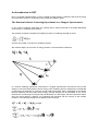
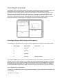
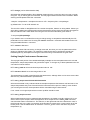
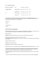
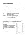
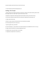
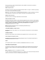
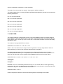
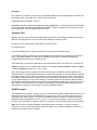
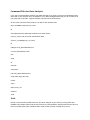
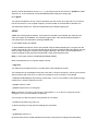
HET Manual AN INTRODUCTION TO HET .......................................................................................................................... 2 THE NEUTRON INELASTIC SCATTERING EXPERIMENT ON A CHOPPER SPECTROMETER ............................................................ 2 COMPONENTS OF A CHOPPER SPECTROMETER. ............................................................................................................. 3 CONTROLLING THE INSTRUMENT ................................................................................................................. 5 SELECTING A CHOPPER SLIT PACKAGE AND FREQUENCY .................................................................................................. 5 SETTING THE INCIDENT ENERGY .................................................................................................................................. 6 CHANGE ................................................................................................................................................................ 6 SETTING SAMPLE ENVIRONMENT PARAMETERS ............................................................................................................. 7 DATA COLLECTION COMMANDS ................................................................................................................................. 8 USING COMMAND FILES ........................................................................................................................................... 9 SAMPLE ENVIRONMENT EQUIPMENT ......................................................................................................... 11 THE ORANGE CRYOSTAT ......................................................................................................................................... 11 THE TOP LOADING CCR.......................................................................................................................................... 11 REMOVING A SAMPLE ............................................................................................................................................ 11 LOADING A NEW SAMPLE ....................................................................................................................................... 12 DATA ANALYSIS AND VISUALISATION. ........................................................................................................ 13 HOMER ............................................................................................................................................................. 13 VANADIUM NORMALISATION ................................................................................................................................... 15 ABSOLUTE NORMALISATION .................................................................................................................................... 16 MAPPING FILES ..................................................................................................................................................... 16 5.1.4.MAPPER ................................................................................................................................................... 17 EXAMPLES ........................................................................................................................................................... 17 Example 1 ..................................................................................................................................................... 17 Example 2 ..................................................................................................................................................... 18 MASKING FILES ..................................................................................................................................................... 18 HOMER OUTPUT ................................................................................................................................................. 18 COMMAND FILES FOR DATA ANALYSIS ....................................................................................................... 19 ILIAD. .................................................................................................................................................................. 19 GENIE ................................................................................................................................................................ 20 COLOUR OUTPUT .................................................................................................................................................. 21 PARIS ................................................................................................................................................................ 21 PRSPLOT6 ‐ A QUICK GUIDE .................................................................................................................................. 22 6. SUMMARIES ........................................................................................................................................... 24 INSTRUMENT CONTROL .......................................................................................................................................... 24 DATA ANALYSIS AND VISUALISATION ......................................................................................................................... 24 A FINAL CHECKLIST ................................................................................................................................................ 25 An Introduction to HET
HET is a chopper spectrometers, in which a single incoming energy is selected, and the final energy
and momentum transfer is analysed by time-of-flight and detector angle.
The Neutron Inelastic Scattering Experiment on a Chopper Spectrometer In any neutron scattering experiment, the quantity that is being measured is the partial differential
cross section, is scattering cross section.
The quantity of interest is actually the scattering function or scattering law S(Q,ω) where
and N is the number of nuclei in the scattering system.
We measure S(Q,ω) as a function of energy transfer ω and momentum transfer Q.
In a neutron scattering experiment conducted on a chopper spectrometer, the neutrons arrive at the
sample in monochromatic pulses of known energy. After scattering from the sample they are detected
in fixed arrays of detectors as a function of their total time-of-flight. With a knowledge of the sample
detector distances and the incident beam energy, the final energies can be calculated. At any one of
the detectors a wide range of energies may be absorbed. For all energies, the final wavevector will lie
along the same direction, however, the magnitude will decrease with the velocity of the incident
neutrons. The scattering triangle is thus altered in time as shown.
By applying the cosine rule to the scattering triangle, bearing in mind that ki is fixed and translating
into energy units, it can be clearly seen that a detector positioned at a scattering angle f will perform a
scan in time whose loci is a parabola in Q,w space.
The scan performed by each detector is dictated by the scattering angle of that detector and the
incident energy.
Components of a Chopper Spectrometer. The components of a chopper spectrometer such as HET are shown in the schematic diagram.
Alongside are examples of the neutron spectra at each point along the path of the neutron. The
proton pulse hitting the target produces a burst of very fast, very high energy neutrons. To slow these
down to usable energies the high scattering cross section of hydrogen is utilised. Hydrogen at 22K,
CH2 at 100K and H2O at 316K are used as moderators. In order to preserve the high flux of high
energy neutrons which is a valuable feature of pulsed sources the beam is undermoderated. That is
to say the neutron flux leaving the moderator has two components; the Maxwellian component
caused by the moderation and the epithermal (high energy flux) of the weakly moderated neutrons.
Figure 1 Schematic diagram of a chopper spectrometer.
A substantial amount of background arises from gamma rays
when the proton beam hits the target and from fast neutrons
which thermalise within the spectrometer. Consequently the
background is reduced significantly by using a nimonic chopper
which effectively closes the beam tube to the spectrometer at the
moment the proton beam is incident on the target.
The beam itself is monochromated by a Fermi chopper, which is
an aluminium drum with thin sheets of highly absorbing material
such as boron, interleaved with neutronically transparent sheets
of aluminium. The rotation of the drum is phased to the ISIS pulse
and is only in transmitting position at the point at which it will only
transmit neutrons with the desired velocity and hence ki and Ei.
In practice the slits are curved in opposition to the direction of
rotation to optimise transmission. The chopper drum becomes
increasingly grey as the energy increases. This greyness gives
rise to a modulated background. This has been reduced by
installing B4C cheeks in the chopper bodies, but still needs to be
accounted for when analysing data.
Monitors are located at the positions indicated on the schematic
diagram of the spectrometer. The time-of-flight between monitors
2 and 3 is used to determine the incident energy.
The sample is mounted on a variety of sample environment
including cryostats, pressure cells and furnaces all with a
standard 17" Tomkinson flange. The tank itself is evacuated to a
cryogenic vacuum during an experiment. The beam tubes and
detector tanks are evacuated to a rough vacuum thus reducing
the background arising from air scattering.
The size of the neutron beam falling on the sample is determined
by the extent to which the beam has been collimated and
apertures at the entry to the sample tank. The final aperture may
be altered by changing the final collimation piece. In the near
future, motorised jaws will be installed to allow tailoring of the beam dimensions to suit the sample
and sample environment.
All internal surfaces in the sample tank are lined with a low hydrogen B4C resin mix which minimises
the background arising from the scattering of high energy neutrons. B4C is also used as a shield
behind the detectors.
HET is equipped solely with 10 atmosphere 3He detectors. The specifications of HET as of February
1994 are summarised in the table in section 7.
Controlling the Instrument
The terminal in the cabin usually displays five windows, conventionally arranged as shown below. The
dashboard at the top left hand corner of the screen provides a display of all the instrument
parameters, including sample temperature goniometer angles etc. Where possible, the HET control
window should only be used for control commands such as beginning, updating and ending runs,
changing incident energies or temperatures, and starting instrument control command files. If this
convention is adhered to it is easy to follow the status of the instrument. All data analysis should be
performed in the HET terminal window. The GENIE windows are used for data display.
Selecting a Chopper Slit Package and Frequency
Four chopper slit packages are used on HET, and their specification are given in the following table.
Slit package
Optimum Ei
A
500 meV
B
250 meV
C
100 meV
S
500 meV
Comments
relaxed resolution
The program CHOP, written by Toby Perring, calculates the flux and resolution expected for a given
chopper running at a given frequency. It has been well documented elsewhere and will only be briefly
described here. To run the program use the HET Terminal window, and type CHOP. You will then be
prompted to give the instrument name. The chopper frequency is often given in terms of multiples of
the ISIS pulse (50Hz). At the arrow prompt you select a chopper and frequency using the command
> s c <frequency/isis> <slit package>
For example, s c 10b selects the B chopper spinning at 500Hz. To plot out the flux and resolution use
the command
> p c <Ei min> <Ei max>
Another chopper can now be selected using the s c command and plotted on the same axis using the
command
>poc
To obtain values for the resolution and flux for a particular slit package and frequency at a specific
incident energy, select the slit package and frequency as before, then set the incident energy using
the command
>set ei <Ei>
The flux and resolution can then be displayed using the commands
>d f
and
>d r
respectively. The command to leave chop is ex.
Setting the Incident Energy To set the incident energy use the command
HET>set_ei <Ei(meV)> <frequency(Hz)> <slit package>
This command will set the necessary phase and frequency, and also write the file, TCB.DAT, which
will be loaded into the instrument control program (ICP) the next time a change or load command is
issued. For this reason, it is crucial that a change command is issued after the energy is set. It is also
vital that the set_ei command is issued from the het$disk0:[het.run] area and that the change or load
command is issued from the same area. The LED display on the chopper control crate in the
instrument cabin displays the chopper frequency and the small LED to the left will be alight until the
chopper has phased correctly. Wait until the correct chopper frequency has been established and the
phase is correct before starting a run. If the phase LED is still alight more than 30 seconds after the
desired frequency has been established, move the small switch below the frequency display from
comp. to man., press the enter data button and return the switch to the comp. position. If the light is
still on inform your local contact.
Once a run has started, it is possible to check that the chopper has phased correctly to give the
desired incident energy using the following commands in the Control window.
HET>update
HET>ei crpt
The ei command calculates Ei from the arrival of the elastic line at monitor three, it can also be used
to find the incident energy of an earlier run by simply giving the run number rather than typing CRPT.
Change The change command allows the user to edit the dashboard information and to modify the ICP
parameters.
Typing the command
HET>change (can be abbreviated to cha)
will initiate the dashboard editor. Move between areas using the cursor keys and over type or toggle,
using the . key on the keypad, as instructed. The first page contains title and user information. When
entering the title please follow the convention
<sample> <temperature> <sample environment> <Ei> <frequency/isis> <slit package>
eg YBa2Cu3O7 T=14K CCR 100meV 10c
The rest of the editor is straightforward. Do not alter the spectra, detector or wiring tables. Unless you
are making a white beam measurement ensure that the bar half way down the last page is toggled so
that the TCB.DAT file is read rather than using the time channel information given below it.
To exit press [PF1(GOLD)] e.
If you intend to set a command file running to change energy or temperature automatically the ICP
parameters can be written to a file using the nextrun <filename> command and loaded into the ICP
using the load <filename> command.
HET> nextrun <filename>
will have the same effect as issuing a change command, but when you exit, the parameters will be
written to <filename>.dat. Again, it is important to make sure that this command is issued from
het$disk0:[het.run]. Examples of running the instrument using command files are given later.
Setting Sample Environment Parameters The top right hand portion of the dashboard displays sample environment parameters such as head
temperature, sample temperature and goniometer angles. To change any of these parameters the set
command is used as follows.
HET>cset t_head 10 will set the head requested value to 10K
HET>cset wccr 45 will move the omega table to 45º
The temperature is usually controlled using the head sensor, although limits can be set to ensure that
data are only collected between specified limits.
HET>cset t_samp/control/lolimit=40/hilimit=50 45
will ensure that data is only collected while the sample temperature lies between 40K and 50K. If the
sample temperature strays out of these limits the instrument will be put into "waiting" mode. Unless
you are using the furnace, the temperature will be controlled using the head sensor.
If run control is no longer required the nocontrol qualifier should be used
HET>cset t_samp/nocontrol
When measurements are to be made at base temperature, the heater is usually switched off. If you
want to warm up the sample, and there appears to be no response to the cset t_head command,
check that the heater is switched on. The switch is on the right hand side of the Eurotherm crate, in
the left hand rack in the cabin. On the back of the Eurotherm crate there is a rotary switch to set the
heater power. Use the tables below for reference. The max_power is set in the same way as the
temperature, eg.
HET> cset max_power 50
Maximum Temperature
10K
30K 50K 150K 300K
orange cryostat
Heater Voltage
24V 46V 52V
60V
72V
max_power
50
50
100
Heater Voltage
12V 24V 32V
60V
72V
max_power
50
100
100
ccr
50
50
100 100
The variation of the head and sample temperatures over time can be studied by plotting the
temperature logs using GENIE. The following set of commands in GENIE will load the sample, then
the head log files and plot both on the same axes.
>>@g:t_cur
>>d/l w1
>>@g:t_head_cur
>>p/l w1
Data Collection Commands All the following instrument control commands may be abbreviated to three letters. Instrument control
commands should be issued form the CONTROL window whenever possible.
begin Starts a run.
update Stores the data collected so far in the current run parameter table (CRPT).
store Stores the data collected up to the last update in the file
HET$DISK0:[HETMGR.DATA]HET0<run no.>.SAV. The store command should always be preceded
by an update.
pause Pauses data collection.
resume Resumes data collection.
abort Aborts the current run without saving any data.
end Ends the current run and stores the data in HET$DISK0:[HETMGR.DATA]HET0<run no.>.RAW.
A command file, UPD_UAMP, will perform an update and a store at given intervals in total beam
current. This will ensure that you will not loose all your data if there are any problems with the DAE
during the run. Run UPD_UAMP from the Control window using the command
HET>@upd_uamp <current at first update> <interval between updates in Amphrs> <current at final
update>
To stop the command file before the final value for the total current has been reached type [Ctrl]Y
Using Command Files Command files can be written to control the instrument. An example command file follows
$ set def het$disk0:[het.run] sets the default directory
$ on error then continue ensures that the command file will continue in the event of a CAMAC error
$ waitfor 700 uamps waits until the total current reaches 700Amps
$ end end the current run
$ cset t_head 80 sets the head temperature
$ cset t_samp/control/lolimit=75/hilimit=85 80 sets temperature limits
$ wait 00:40:00 waits 40 mins for the temperature to stabilise
$ load ndnio_80.dat loads the new icp parameters which have been written to the file ndnio_80.dat as
described in section 2.3.
$ begin begins the next run
$ waitfor 500 uamps
$ update
$ store
$ waitfor 700 uamps
$ end
$ set_ei 100 250 c sets Ei for the next run
$ wait 00:15:00 waits 15 mins for the chopper to phase
$ load ndnio_100.dat
$ begin
$ waitfor 700 uamps
$ exit leaves the command file
A command file can be run from the terminal using @<filename> or as a batch job on the HET slow
queue. The advantage of using a batch job is that it is possible to stop, start and alter a command file
remotely. The disadvantage is that it is not obvious to anybody sitting at the instrument terminal that
the instrument is being controlled by a command file. Please run all command files, and start batch
jobs, from the Control window to reduce the chances of confusion.
To submit a batch job use the symbol shq thus;
HET>shq <filename>.
Check that the file is being executed by viewing the queue
HET>qh
To stop a batch job use the halt command
HET> halt <entry no.> het$slow
The entry number identifies the job and is displayed with the queue information. The progress of the
command file can be monitored by viewing the log file, which is written to SYS$SCRATCH. Use the
type command as follows
HET>ty sys$scratch:<filename>.log.
Note: SYS$SCRATCH: is the logical name for SCRATCH$DISK:[<user id>] and may be shortened to
SS
Sample Environment Equipment
The two most commonly used pieces of equipment on HET are the orange cryostat and the top
loading ccr.
The Orange Cryostat The use of the orange cryostat is described in RAL reports 93-006 and 92-041, copies of which are
kept in the HET cabin. The table below provides brief information concerning valve settings and flow
rates. Both the warm and cold valves should only be finger tight. Over tightening them will cause
damage.
Cooling to
>4K
Open the cold valve 1/2 turn. Open the warm valve until the
flow observed on the gas recovery flow meter is 10L/min
Constant
temperature
>4K
Once the required temperature has been reached reduce
the flow to approximately 4L/min using the warm valve, and
the temperature will be controlled by the Eurotherm and the
cryostat heater, or, if you want the temperature to remain
stable at 4K, switch the heater off.
Cooling to
<4K
Close the warm valve, and open the cold valve 1/2 turn.
Slowly open the Rootes pump valve, never letting the
pressure rise to above 10 torr. When the pump valve is fully
open use the cold valve to adjust the flow.
The Top Loading CCR
Installing the top loading ccr will have to be done by the local contact, however changing samples is
very straightforward, but demands care, because there is the potential to open the sample tank to air
very rapidly which will destroy the thin window between the sample and detector tanks.
Removing a Sample 1. Undo the sample sensor connector (1) from the top of
the samplestick.
2. Undo the clamp (2) on the tightening rod (3), and lower
it until it engages with the allen head bolt (4) which holds
the sample holder to the cold head and unscrew it
3. Lift the sample by pulling the plate (5) all the way up
the two tubes and secure it at the top with an allen screw
(6).
4. Close the gate valve (7).
5. Loosen the three bolts which hold the plate onto the
top of the air-lock (8).
6. Open the speed valve which lets air into the air-lock (9).
7. Undo the bolts (8) and lift the sample stick out.
Loading a New Sample 1. Before replacing the sample stick place a small piece of indium wire round the bolt (4) that secures
the sample holder to the cold head to improve the thermal contact.
2. Replace the sample stick and finger tighten the three bolts securing it to the air-lock (8).
3. Close the air-admittance speed valve (9), and open the speed valve to the pump (10).
4. Tighten the three bolts (8).
5. WAIT for a few minutes to ensure that the air-lock has been evacuated
6. Close the speed valve to the pump (10).
7. Open the gate valve (7) SLOWLY.
8. Lower the sample (11) into position. Ensure that the plate (5) is pushed down as far as it can go.
9. Tighten the allen head bolt (4) using the tightening rod (3).
10. Withdraw the rod (3) and camp it (2) in position.
11. Replace the sample sensor connector (1).
Data Analysis and Visualisation.
Several programs and utilities exist to help you analyse your data including the FRILLS least squares
fitting program. There is only scope here to provide the information required to allow you to produce
S(,) plots of your data, more detailed information will be available shortly, and copies of the FRILLS
manual are available. If you are doing your data analysis in your own directory make sure that you are
using the HET login.com. If you are analysing data sometime after the experiment take care to
explicitly state par files, using the /PAR qualifiers when running DIAG and WHITE_VAN, and mapping
files, using the /MAP qualifier, when running HOMER. The default files are modified whenever the
detector arrangement is altered. Make sure you make a note of the names of the mapping and par
files that were in use when your data was collected.
The program HEAD is very useful if you want to find out the title, running time and total current of a
previous run. It has the format
HET>head <run no.>
Figure 3 is a schematic layout of the HET detectors. Each detector is assigned a particular spectrum
number. In most cases spectra are summed into workspaces. The rings drawn on figure 1 represent
the default workspaces numbered 1 to 7 and the average angle for each workspace is given.
HOMER The data analysis program for HET data is HOMER, which performs the following functions.
It reads in raw data stored either in disk files (RAW or SAV files) or in the FEM memory (CRPT).
The incident energy is automatically determined from the measured monitor spectra.
The data are grouped into workspaces defined by a mapping file.
Noisy or unstable detectors can be eliminated from workspaces using a mask file. This feature also
allows the elimination of detectors picking up Bragg or spurious scattering
A time-modulated or time-independent background, determined from the end of the time frame, is
subtracted from the workspaces.
The data is converted to S(f,w) i.e. converted to energy transfer and corrected for kf/ki and detector
efficiency.
HOMER results are usually stored in a binary file in the GENIE intermediate file format, to allow
subsequent analysis within GENIE. If preferred, the workspace information can be written to an ASCII
file
An ASCII diagnostics file containing details of the HOMER analysis (incident energies, monitor
integrals, spectrum integrals and backgrounds etc.) can be produced.
Figure 3. The HET detector layout, showing spectrum numbers, and default HOMER workspaces and
their average values.
The format of the command is
HOMER <data source> (<Ei> (<Emin> (<Emax> (<dE>))))
As with all DCL commands, the user may give the shortest unambiguous abbreviation which is
usually HO. The user may modify the options used by HOMER by including qualifiers in the command
line. e.g.
HO/MAP=MAP:ARMS_911/MASK/VAN=2414/CHOP=400 2420
The most commonly used are described below. Other qualifiers are normally only required in
exceptional circumstances.
/MAP=<map file name>
Specifies the spectrum mapping file with default extension MAP. If not given, a default ring mapping
file is used (currently MAP:RINGS_934.MAP).
Note MAP: is the logical name for HET$DISK:[HETMGR.MAPS]. It contains a number of commonly
used mapping files. The file AAA.TXT contains a description of the mapping files in MAP:
/MASK=<mask file name>
Specifies a spectrum masking file. Mask files are discussed later
/VAN=<vanadium sum file>
Specifies a white-beam vanadium sum file containing integrals from 20 to 40 meV for each detector,
normalised to a default M1 sum. The integrals are used to normalise for the solid angle and detector
efficiency prefactor for each detector. The sum file is either specified in full or just given as a run
number, in which case the default file name is HET_DATA:HET0<run no.>.SUM or
SYS$SCRATCH:HET0<run no.>.SUM.
Note HET_DATA: is the logical name for HET$DISK0:[HETMGR.DATA] or
HET$DISK:[HETMGR.DATA].
/CHOP(PER_SPEED)=<chopper speed>
Specifies the speed of the chopper in Hz. This is required for the subtraction of a time modulated
background.
/NORM(ALIZATION)
Determines if the data are to be normalised to the integrated monitor counts or proton current.
/OUT=<diagnostic output file name>
Specifies the name of the ASCII file containing diagnostic output. The default file specification is
SYS$SCRATCH:HET0<run no.>.OUT.
/ASCII
The workspace data is written to an ASCII file, SYS$SCRATCH:HET0<run no.>.DAT.
Vanadium Normalisation The white beam vanadium sum files, required by HOMER for normalisation and by the diagnostic
program to create a mask file are created by the program WHITE_VAN. The command has the
format.
White_van(/par=(<par file no.>) <vanadium run number>
This will create a file SYS$SCRATCH:HET0<run no.>.SUM. A copy of this file will usually have been
copied by the instrument scientist to HET$DISK:[HETMGR.DATA].
Absolute normalisation Scattering intensities can be put on an absolute scale in mbmeVsr-1 using the /ABS qualifier and
calculating a constant for the normalisation from the data collected for a monochromatic vanadium run
The monochromatic vanadium data should be summed over the elastic peak using SUM as follows
SUM(/PAR=<par file no.>)/CHOP=<chopper frequency (Hz)>/VAN=<w.b. run no.>/NORM/COR
<monochromatic van. run no.> <-xlimit> <+xlimit>
The x limits are in meV energy transfer and should be set to include all the elastic scattering from the
vanadium. These values are estimated by inspecting the monochromatic vanadium data after it has
been HOMERed. The qualifiers have the same meaning as they have for HOMER, except for /COR
which stipulates that the data should be corrected for detector efficiency.
The summed data can now be used to derive the constant for normalisation, including the mass of the
vanadium, the mass of the sample and the atomic mass of the sample. This is done using the
MONO_VAN program as follows.
MONO_VAN/MV=<mass of the vanadium sample (20.14g)>/MS=<mass of the sample>/AS=<atomic
mass of the sample> <monochromatic van. run no.>
The number calculated in this fashion is given the variable name MONO_COR and needs to be
trimmed before being used in the HOMER command. This is done by the command
MONO_COR=F$EDIT(MONO_COR,"TRIM")
Absolute values for the scattering will now be produced if the qualifier /ABS='MONO_COR' is used in
the HOMER command.
This process is made considerably easier if you use a command file to perform all the steps of the
analysis. An example is given in section 4.2.
Mapping files HOMER groups the recorded spectra into workspaces according to a mapping file, which is either
specified by the /MAP qualifier or defined by the default value set in the current HOMER command
table.
The mapping file is an ASCII file containing the following lines in free format:
1st Line: Nw Nw = No. of workspaces in map
2nd Line: Nsp, L2,t, Nsp = No. of spectra in first workspace
L2 = Length of scattered flight path of first workspace (in m)
t = Electronic time delay of detectors in first workspace
(in ms)
= Average scattering angle of first workspace (in º)
3rd Line: List of spectrum nos. in first workspace (N.B. 3-9 is read as 3,4,5,6,7,8,9)
4th line: Continuation of spectrum no. list if necessary:
The pattern, from the second line onwards, is repeated for all Nw workspaces.
The default mapping file is currently HET$DISK:[HETMGR.MAPS]RINGS_943.MAP which defines the
following workspaces:
W1 4.9º 4m low angle bank
W2 11.5º 2.5m low angle bank
W3 16.5º 2.5m low angle bank
W4 21.5º 2.5m low angle bank
W5 26.5º 2.5m low angle bank
W6 115.0º 4m high angle bank
W7 133.0º 2.5m high angle bank
5.1.4.MAPPER This program produces a mapping file for use on HET with HOMER (It does not produces mapping
files for MARI). It allows the spectra from the low angle 4 meter detector bank, the medium angle 2.5
meter detector bank, and the high angle 4 meter and 2.5 meter detector banks to all have individually
definable bin sizes.
The method of running MAPPER is as follows:$ MAPPER <run number> <L> <M> <H1> <H2>
Where L,M,H1 and H2 are the low angle, medium angle and the two high angle detector bank bin
sizes respectively, in terms of the number of detectors thick a ring will be.
The default input parameter file for this operation is the default .par file which can be found in
HET$DISK:[HETMGR.DATA]. If it is required that input to MAPPER should be from a parameter file
other than the default file, then the qualifier /PAR=number should be used, as shown below:$ MAPPER/PAR=<number> <run number> <L> <M> <H1> <H2>
Examples Example 1 MAPPER is to be run with default parameter file input, for run number 4660. The low angle binning
required is 5, the medium angle binning is 16, the high angle 4 meter binning is 22 and the high angle
2.5 meter binning is 11. The command line is as follows:$ MAPPER 4660 5 16 22 11
Note the single space after the command and the single space separating each number!
Example 2 The values from example 1 are the same, except that a different input parameter file is required. The
file needed is HET_955.PAR. The command line is as follows:$ MAPPER/PAR=955 4660 5 16 22 11
MAPPER produces a mapping file called HET0run_number.MAP, so for the previous two examples,
in both cases the output file would be HET04660.MAP. This file is written to the scratch disk, so the
final mapping file is SS:HET04660.MAP in this case.
Masking Files Masking files are used to eliminate small numbers of detectors from workspaces without the need to
define a new mapping file. Common reasons for masking a detector are that
its efficiency has varied between white beam vanadium counts
it is relatively noisy
it contains a Bragg peak or spurious scattering contaminating the inelastic signal.
The masking file simply consists of a list of masked spectra in free format occupying any number of
lines. If the /MASK qualifier is used with the HOMER command then the default masking file
(SYS$SCRATCH:HET0<run no.>.MSK) is used.
The easiest way to generate a mask file is to use the program DIAG. The format of the command is
diag/v1=<vanadium run no.>(/v2=<2nd vanadium run number>)(/nozero)(/stab=< stability>)(/factor
=<factor>)/out(/par=<par file no.>) <run no./crpt>
DIAG will compare the two vanadium sum files and identify those detectors whose efficiency has
varied between the runs and add the spectrum numbers of those detectors to the mask file, providing
the /OUT qualifier is used. If the /OUT qualifier is not used, the file will not be written. It will compare
the stability of detectors within a vanadium sum file and include those detectors which produce a low
or high signal relative to a norm in the mask file. The data will then be searched for detectors with a
high background and these will also be excluded. If the /NOZERO qualifier is not used those spectra
that contain no counts will also be excluded. It is advisable to use the /NOZERO qualifier until the
data has been counted for long enough to provide reasonable statistics.
HOMER output The workspaces are stored in a binary file in the format required by the GENIE READ command. The
default file name for this file is SYS$SCRATCH:<inst><run no>.COR. The name of this file may be
changed by the /COR qualifier. A record of the HOMER analysis is stored in an ASCII file with the
default file name SYS$SCRATCH:<inst><run no>.OUT if the /OUT qualifier is used. In both cases,
the files may be directed to a different directory but with the same file names using the /DIR qualifier.
Note: Files stored on SCRATCH$DISK: will be deleted after one week, so if longer storage is
required, you must use the /DIR qualifier, which will allow you to stipulate a destination directory, or
rename the files after running HOMER.
Command Files for Data Analysis
If you use a command file to analyse your data and keep it you have a record of the parameters and
files used in your analysis. Also, re-analysis of your data is straightforward and you do not have to fill
you quota with .COR files. A typical analysis command file is shown below.
$! This is the command file to produce .cor files for the 100meV data
$! for the NdNiO3 expt January 1994.
$!
$ sum/par=932/van=4293/chop=500/norm/cor 4309 -50 50
$ mono_van/mv=20.14/ms=36.5/as=250.95 4309
$ mono_cor=f$edit(mono_cor,"trim")
$!
$ diag/v1=het_data:het04293.sum/v1=het_data:het04310.sum/out4305
$!
$ homer/chop=500/van=het_data:het04293.sum/map=map:rings_934.map/mask/norm/abs='mono_cor'
/norebin4305
Iliad. Iliad is a command file that will perform a "first look" analysis of your data, by running DIAG and
HOMER using default values and the most commonly used qualifiers. Iliad requires the sum file from
the most recent white beam vanadium data. If this file has not been created you must run
WHITE_VAN as described in section 4.1.1.. If you intend to look at the current run update the CRPT
(section 2.5). In the instrument control (HET$DISK0:[HET.RUN]) area simply type
HET>@iliad.
You will be prompted for the run number of the data you wish to look at or type CRPT if you want to
look at the current run, the chopper frequency and the number of the white beam vanadium run.
The data will be written to a .COR file as described by the default mapping file.
GENIE GENIE is the ISIS graphics software. A full manual is included in the PUNCH user manual in the
cabin and copies are available in the computer support office. Here we will briefly describe the
commands which are essential for viewing HOMER data.
To run GENIE simply type GENIE.
To load HOMER workspaces, which were created using the default mapping file, into genie use the
g:read command file. This command file will read in the seven workspaces described earlier and also
write an eighth workspace containing the average scattering in the whole 2.5m low angle bank. If
another mapping file was used the command file g:read_work should be used.
Note g: is the logical name for HET$DISK:[HETMGR.GENIE].
Both command files are run in genie using the format
>>@g:read
You will then be prompted for the run number and the first workspace number
The workspaces can be displayed using the command d. The plot command, p, allows you to plot the
data as markers with error bars, or to plot one workspace on top of another. For example
>>d/m w1 -10 90 0 20 plots the intensity of workspace 1 from 0 to 20 (arbitrary units) against energy
transfer from -10meV to 90meV as marks.
>>p/e w1 adds error bars
>>p/h w2 overplots w2 as a histogram
Note d produces a new plot, p will overplot. The qualifiers, /l, /h, /e and /m correspond to lines,
histograms, error bars and markers respectively.
You may bin you data into groups using the alter bin command;
>>a b 5 bins the data into groups of 5
To take a hardcopy of a plot use the following two commands
>>k/h
>>j post<laser printer no.>
where the laser printer number identifies the location of the printer according to the table below.
laser printer number
0
1
2
11
location
Computer support office, R3.
Coffee room, R3.
DAC, R55.
HET cabin
For example, to print on the HET laser printer use
>>j post11
Once you have plotted one workspace to your satisfaction, the command file g:precis will
automatically plot with error bars all eight workspaces and print them all on a single sheet of A4 on
the HET laser printer. Precis divides workspaces 6 and 7 by five. This is an empirical figure which
allows you to estimate the effects of non-magnetic background scattering on the data collected in the
forward scattering banks.
Colour Output Data can also be displayed as a colour contour S(Q,w) plot using the PRSPLOT package, which has
it's own manual. It also allows energy and Q cuts to be plotted, rather than the constant cuts usually
viewed when HOMERed data is read into GENIE. Mapping files which use finer rings than the default
file are usually required for a contour plot. these can be created using MAPPER. To prepare data to
be plotted using PRSPLOT6 it should be HOMERed as described above, but with the /ASCII qualifier
to produce a file named ss:HET0<run number>.dat. This file can be converted for PRSPOT6 using
the program CONVERT as follows.
HET>CONVERT <run number>
e.g. HET>CONVERT 2136
This operation produces an output file called HET0<run number>.CON, so the above command would
produce a file called HET02136.CON, which will be written to SCRATCH$DISK, (SS): which means
that the full file name would be SS:HET02136.CON.
To produce a colour plot, simply type PRSPLOT6, so the command line will be:HET>PRSPLOT6
You may now refer to "PRSPLOT6 - a quick guide to colour output" which follows after the next
section.
PARIS A command file called PARIS.COM exists which will allow you to produce colour data plots, without
allowing any default settings to be altered. PARIS will prompt you for all the relevant information at the
start, and it will then run the following programs :- DIAG, MAPPER, HOMER and CONVERT. You
then simply need to run PRSPLOT6 to plot the data. The complete sequence is as follows :HET>@PARIS
PARIS will now run, and produce the following prompts. The values in italics are an example of user
input.
Enter current run number or crpt to look at current run : 4822
Enter chopper frequency in Hz : 550
Enter white beam vanadium run number : 4758
Enter Ei : 80
Enter Minimum hw : -20
Enter Maximum hw : 75
Enter h step size : 0.5
Enter Low Angle Bin Size : 2
Enter Medium Angle Bin Size : 5
Enter High Angle 4 meter Bin Size : 11
Enter High Angle 2.5 meter Bin Size : 11
In the above list, Ei is the incident neutron energy in meV.
To produce a colour plot, use PRSPLOT6. The command line is :HET>PRSPLOT6
PRSPLOT6 ­ A quick guide After the PRSPLOT6 command has been entered, the program will run and give you the following
prompts. The suggested replies appear in bold and should be followed by carriage return <CR>.
Enter terminal type : 2 <CR>
Enter the hardcopy device output file type : 2 <CR>
Which font do you want ? [SIMP] : <CR>
You will now reach the PRSPLOT6 command line, and should type :
> L W1 filename <CR>
e.g. > L W1 SS:HET02136.CON <CR>
Now answer the prompts. The data type is 5 and the scan is a CD scan. On HET normalistaion is
done by HOMER, so we do not use a normalisation file. Contour levels can be set using the A/H I
command.
You may now plot the data with the command line :> D/S W1 <Qmin> <Qmax> <Emin> <Emax>
To print a plot simply enter s. A postscript file will be created in the current directory called post.dat.
Thsi file may be printed on the colour printer in the support office using the command
HET> COL POST.DAT
Alternatively, use the inkjets printers in the DAC or the MARI cabin with the relevant ink command.
(The DAC printer is INK2, the MARI printer INK3). For more detail on PRSPLOT6, please refer to the
PRSPLOT6 manual.
6. SUMMARIES
Instrument Control The following sequence represents the commands required to start a typical run.
HET Control HET>tt het.run 0 Ensure that set_ei and change are issued from het$disk0:[het.run]
HET>set_ei <Ei(meV)> <freq. (Hz)> <slit package> eg. set_ei 100 250 c
HET>cset t_head <temp> set the requested head temp.
HET>cha
Over type new title, parameters etc.
[PF1] e
HET>beg start the run
HET>upd update
HET>ei crpt Check that Ei is correct
HET>@upd_uamp 500 500 Run a command file to update and store at 500 Amp intervals
.
.
.
[Ctrl] y Stop the command file
HET> end End the run
Data Analysis and Visualisation The following sequence will allow you to produce S(,) plots of your data, using the default settings.
HET Control
HET>update or end
HET Terminal
(HET>White_van <1st van run no.>
HET>White_van <2nd van run no.>)
HET>diag/v1=<1st van run no.>/(v2=<2nd van run no.>)/out(/nozero) <crpt or run no.>
HET>Ho/chop=<freq (Hz)>/norm/van=<van run no.>/mask/norebin <crpt or run no.>
(or use ILIAD)
GENIE
>>@g:read Will read in HOMER workspaces
run number :<run no.>
First workspace: :1
>> d/m w<workspace> xmin xmax ymin ymax Display the given workspace
>> a b <bin> Bin the data into groups of 'bin'
>> d/m
>> p/e Plot error bars
>> k/h Keep a hardcopy
>> j post11 Print on the HET laser printer
>> @g:precis Will plot all eight workspace and print them on a single A4 sheet
A Final Checklist Before you walk out of the cabin for a quiet night in the pub, quickly go through the following checklist.
Interlocks complete
Shutter open
Vacuum good (<1mb)
set_ei and cha issued from het$disk0:[het.run]
Chopper correctly phased (update, ei crpt)
Heater on (if necessary)
Command file for automatic update and store running
or
Overnight command file or batch job running